accepted by journal selected topics quantum electronics, vol… · · 2013-02-04accepted by...

accepted by JOURNAL SELECTED TOPICS QUANTUM ELECTRONICS, VOL. 19, NO. 5, SEPTEMBER/OCTOBER 2013 1

Basic aspects of high-power semiconductor lasersimulation

Hans Wenzel

(Invited Paper)

Abstract—The aim of this paper is to review some of the modelsand solution techniques used in the simulation of high-powersemiconductor lasers and to address open questions. We discusssome of the peculiarities in the description of the optical fieldof wide-aperture lasers. As an example, the role of the substrateas a competing waveguide in GaAs-based lasers is studied. Thegoverning equations for the investigation of modal instabilitiesand filamentation effects are presented and the impact of thethermal-lensing effect on the spatiotemporal behavior of theoptical field is demonstrated. We reveal the factors that limit theoutput power at very high injecton currents based on a numericalsolution of the thermodynamic based drift-diffusion equationsand elucidate the role of longitudinal spatial holeburning.

I. INTRODUCTION

TREMENDOUS advancements have been achieved in thedevelopment of high-power semiconductor lasers during

the last two decades, due to improved cavity design, crystalgrowth, facet passivation, and device cooling technologies[1]–[6]. The output power has increased by one order ofmagnitude, the spectral linewidth has decreased thanks toBragg gratings integrated into the cavity, and the beam qualityhas greatly improved thanks to tapered gain regions. Semi-conductor lasers are under the way not longer to serve onlyas optical pumps for solid-state lasers but to replace thembecause of their ease-of-use, compactness, efficiency and highreliability. However, many of the parameters of high-powersemiconductor lasers are still far from what is achievable fromsolid-state lasers.

For example, the reliable maximum output power is cur-rently limited to values below 20 W from a 100-µm stripewidth device and a further increase remains an open challenge.High-power semiconductor lasers are also plagued by theappearance of multiple peaks in the lateral far- and near fieldprofiles as well as in the optical spectrum in particular athigh injection currents. These effects are caused by modalinstabilities or by lasing filaments formed by a self-focusingmechanism where the refractive index locally increases inregions of high optical intensity.

In order to assess the root causes of these limitationsphysics-based modeling and numerical simulation is moreimportant than ever. The aim of this paper is to reviewsome of the models and solution techniques used in the

H. Wenzel is with the Ferdinand-Braun-Institut, Leibniz-Institut furHochstfrequenztechnik, Gustav-Kirchhoff-Str. 4, 12489 Berlin, Germany, e-mail: [email protected]

Manuscript received November 27, 2012; revised January 22, 2013.

simulation of high-power semiconductor lasers and to addressopen questions.

The paper is organized as follows. We will start in SectionII with a model for the optical field and introduce conceptssuch as the paraxial parabolic equation, roundtrip operator andmodes. In Section III we discuss the modeling of the nonlinearinteraction between the optical field and the injected carriers inhigh-power lasers leading to a non-stationary behavior of thefield pattern. The simulation of the stationary electro-opticalcharacteristics of high-power lasers using the thermodynamicbased drift-diffusion (or energy transport) model will be pre-sented in Section IV. We end with a summary and outlook.

II. DESCRIPTION OF THE OPTICAL FIELD

A. Paraxial parabolic equation

The optical field in edge-emitting semiconductor lasers canbe well described by the paraxial parabolic equations [7]

−ik0nng

cβ0

∂E±

∂t∓ i∂E

±

∂z+

1

2β0∆tE

±

+k2

0n2 − β2

0

2β0E± +

k20ξ±

2β0E∓ = 0 (1)

for the right and left traveling waves E+ and E−, respectively.Eq. (1) can be derived from Maxwell equations with theAnsatz

E(rt, z, t) = ex[E+(rt, z, t)e−iβ0z

+ E−(rt, z, t)e+iβ0z]eiω0t (2)

for the transverse electric field in order to remove the rapidvariations with respect to the time t and the coordinate z alongthe cavity axis, and a corresponding Ansatz for the complexdielectric function,

ε(rt, z, t, ω)|ω0= n2(rt, z, t)

+ ξ+(rt)e−i2β0z + ξ−(rt)e+i2β0z. (3)

In (1-3), rt = (x, y) are the transverse coordinates, ∆t is thetransverse Laplacian, ω0 and β0 are the real-valued referencefrequency and reference propagation factor, respectively, k0 =ω0/c = 2π/λ0 with λ0 being the reference vacuum wave-length and c the vacuum velocity of light, ng = ∂(ωn)/∂ω|ω0

is the group index and ξ± are the Fourier coefficients ofa Bragg grating integrated into the cavity. We have furtherassumed a TE-polarized field with ex being the unity vectorand that the dielectric function varies slowly with respect to

0000–0000/00$00.00 c© 2013 IEEE

arX

iv:1

302.

0173

v1 [

phys

ics.

optic

s] 1

Feb

201

3


x. The distribution of the complex-valued refractive index n(which may include a time dependence much slower than thevariation given by 1/ω0) can be written as

n = nr + ig − α2k0

(4)

with g being the gain due to inter band transition and α theabsorption coefficient due to intraband transitions (e.g. freecarrier absorption).

The temporal dispersion of the dielectric function has beentaken into account only up to the first order in the real partof the refractive index n, higher order dispersion and thedispersion of the imaginary part have to be properly added(see Section III). We should note that in a numerical evaluationof (1) the factor in front of the time-derivative must beapproximated by

k0nng

cβ0≈ 1

vg(5)

with a real-valued group velocity vg.Eqs. (1) must be supplemented by appropriate boundary

conditions. At the plane facets of the laser

E+(0)− r0E−(0) = 0,

E−(L)− rLe−i2β0LE+(L) = 0(6)

hold at z = 0 and z = L, respectively. We should mention thatin the paraxial approximation the facet reflectivities r0 and rLare input parameters which have to be calculated in advance.

At the transverse boundary denoted by Γ one can assume,for example, decaying fields or a perfect electric wall,

lim|rt|→∞

E± = 0 or E±|rt∈Γ = 0, (7)

respectively. If only a part of the cross-section of the cavity issimulated, a non-reflecting or transparent boundary conditionhas to be used which models the fact that only outgoing wavesshould be present. This boundary condition can be formulatedonly in operator form for the general case,

∂E±

dn|rt∈Γ = −iDE±|rt∈Γ (8)

where D is the operator for a so-called Dirichlet-to-Neumannmap [8]. We will consider below in Subsection II-F an examplefor a one-dimensional case. For spatially and temporallyconstant n, D can be obtained by a factorization of (1) [9].A very popular method to implement a boundary condition oftype (8) is the introduction of a so-called perfectly matchedlayer (PML) [10]. However, in the frequency domain it resultsin a large number of spurious modes [11].

B. Cavity modes

The cavity modes are time-periodic solutions of the formE±mexp(iΩmt) and obey the equations

k0nngΩmcβ0

E±m ∓ i∂E±m∂z

+1

2β0∆tE

±m

+k2

0n2 − β2

0

2β0E±m +

k20ξ±

2β0E∓m = 0 (9)

subject to the boundary conditions (6)-(8). The non-trivial so-lutions of (9) may dependent on time via the time-dependenceof n. The complex-valued relative mode frequencies Ωm arethe eigenvalues and the mode profiles E±m(rt, z, t) are theeigenfunctions of (9). Some mathematical properties and theirphysical impact will be discussed below. The real parts of Ωmgive the wavelengths relative to the reference wavelength λ0,

∆λm =dλ

dω

∣∣∣λ0

Re(Ωm) (10)

and the imaginary parts describe the damping of the modes.For a passive cavity, Im(Ωm) > 0 must hold. Lasing modesof an active cavity are distinguished by vanishing damping,Im(Ωm) = 0, due to the balance of the outcoupling andinternal losses and the gain.

The cavity modes fulfill the orthogonality relation∫nng

[E+mE−m′ + E−mE

+m′

]dxdydz = 0 for m 6= m′

(11)which is proven in the Appendix. It is similar to correspondingorthogonality relations for cavity modes derived in [12] and[13] from Maxwell and Helmholtz equations, respectively.

Note that the integral (11) does not define a scalar product[14]. In fact, (9) defines a non-Hermitian eigenvalue problem,because the frequencies Ωm are complex-valued. It is well-known from the theory of non-Hermitian operators, that in de-pendence of some parameter(s) so-called “exceptional points”exist where the eigenvalues (both real and imaginary parts)cross and the eigenfunctions become identical [15]. Mode de-generacies related to exceptional points have been discoveredfor unstable laser cavities, cf. [16] and the references therein,multi-section lasers [17], [18] and complex planar waveguides[19]. Due to the mode degeneracy, at an exceptional point thesystem of eigenfunctions is no longer complete, but a systemincluding the generalized eigenfunctions is, cf. [20].

At the exceptional point, the modes remain orthogonal inthe sense of (11), so that the integral

∫nngE

+mE−mdxdydz

vanishes. As a consequence, Petermann’s K factor [21]

Km =

∣∣∣∣∣∫nng

[|E+m|2 + |E−m|2

]dxdydz

2∫nngE

+mE−mdxdydz

∣∣∣∣∣2

, (12)

approaches infinity. It is known, that the K factor causes anenhancement of the spontaneous emission, which results in abroadening of the spectrum of a multi-longitudinal-mode laserand the spectral linewidth of a single mode as summarized in[22]. Its time-dependence is needed to explain the dynamicalbehavior of multi-section lasers [23].

C. Beam propagation method and roundtrip operator

For a solution of (9) it is convenient to introduce theoperator

H(rt, z) =1

2β0∆t + ∆β (13)

with the abbreviation

∆β =k2

0n2 − β2

0

2β0. (14)


If ξ± = 0 holds (Fabry-Perot cavity), and if the index ndepends only on the transverse coordinates, n = n(rt), thesolution of (9) can be formally written as

E±m(rt, z′) = e∓i(

Ωmvg

+H)(z′−z)E±m(rt, z) (FP cavity),

(15)using the approximation (5). The numerical evaluation of (15)is the basis what is known as the beam propagation method(BPM) [24]–[26]. It has been used for the simulation of bothpassive [27] and active [4], [28], [29] high-power laser cavities.

For the case of a spatially and temporal constant index,n = const., (15) can be evaluated exactly to yield

E±m(r′t, z′) = e∓i(

Ωmvg

+∆β)(z′−z)

×∫G±(r′t − rt, z′ − z)E±m(rt, z)dxdy (FP cavity) (16)

with

G±(r′t − rt, z′ − z) =

Θ(± (z′ − z)

) [√± iβ0

2π(z′ − z)

]2

e∓iβ0|r

′t−rt|2

2(z′−z) (17)

where Θ denotes the Heaviside step function. The integralequation (16) together with the propagator (17) is known asHuygen’s integral in the Fresnel approximation. It has beensuccessfully applied for the simulation of laser cavities asoutlined in [30], [31], including those of semiconductor lasers[32]–[34].

Based on (15) and the boundary conditions (6) it is possibleto construct round trip operators M±. One starts at someposition z = z0 within the cavity and performs a full roundtrip.Depending whether we start into forward (+) or backward (−)directions, the eigenvalue problems

M±E±m(rt, z0) = γmE±m(rt, z0) (18)

are obtained withγm = ei

2Ωmvg

L (19)

being the eigenvalues. The eigenfunctions of M± are the modedistributions E±m(rt, z0) at the position z0.

A very popular method for solving (18) is based on theFox-Li approach, cf. [30] and the references therein. Theidea is to choose a normalized, more or less arbitrary startdistribution E±m(rt, z0) and to apply the round trip operatorM± recurrently until one arrives (hopefully) at a steadystate, i.e. a distribution that does not change its pattern in around-trip, except for a reduction in amplitude and a phaseshift which yields γm. Thereby typically the phase factorexp(− 2iRe(∆β)L− 2iβ0L)

)is omitted.

The Fox-Li approach delivers the mode with the largest|γm| if converged which is, however, not guaranteed. From amathematical point of view, it is related to the power (alsocalled vector or von-Mises) iteration to determine the largesteigenvalue of a matrix and the corresponding eigenvector.It is known, that the generated sequences converge only ifthe eigenvalue is simple and well separated from the othereigenvalues. Hence, the algorithm fails if there are cavitymodes having identical or nearly identical dampings Im(Ωm).

Nowadays, there are more stable and efficient methods to solve(18) for passive laser cavities based on Arnoldi or Lanczositeration. Recently, an alternative approach based on a finite-element method for solving (9) directly, without recourse to(18), has been proposed [35].

Simulations of active laser cavities based on BPMs stillutilize the Fox-Li approach [4], [36], which work quite wellfor single-transverse mode lasers. The approach fails for multi-transverse mode lasers and at high output power if nonlinear-ities such as self-focusing and filamentation start to dominate,cf. [37] for a recent discussion of the stability of the Fox-Liapproach. The association of the nonconvergence of the Fox-Li iteration with an dynamically unstable laser behavior (as in[38]) should be done with care. Instead, for multi-mode high-power lasers, a time-dependent approach based on (1) shouldbe preferred, although numerically more challenging.

D. Beyond paraxial approximation

With improving computer capabilities, direct numerical so-lutions of Maxwell or Helmholtz equations without recourseto the paraxial approximation become more and more fea-sible. For example, in [39] a scalar Helmholtz equation hasbeen solved in the (x, z) (lateral, longitudinal) plane for ahigh-power laser, restricted, however, to short cavities. Annumerical model based on the Helmholtz operator and a first-order time derivative obtained from Maxwell equations byseparating the rapidly varying term exp(iωt) has been used in[40] for the simulation of a monolithically integrated master-oscillator power-amplfier. Another possibility is the expansionin terms of waveguide modes [41], [42] considered in the nextSubsection.

E. Waveguide modes

We can expand the left and right traveling waves in termsof waveguide modes,

E±(rt, z, t) =∑ν

A±ν (z, t)χν(rt, z, t), (20)

which are solution of

∆tχν +[k2

0n2 − β2

ν

]χν = 0 (21)

subject to the boundary conditions (7). The waveguidemodes are exact solutions of Maxwell equations of the formEν(rt)exp(iωt−iβνz) if the dielectric function is translation-ally invariant along z [43].

Eq. (21) is in general a non-hermitian eigenvalue problemfor the complex propagation factor βν . An overview of severalmethods to solve (21) can be found in [25]. Expansion intowaveguide modes allows an exact treatment of waveguidediscontinuities such as Bragg gratings [44] or laser facets [45]in order to calculate their reflectivities. In what follows weintroduce an approximate solution of (21).


0 1 2 3 4 53.35

3.40

3.45

3.50

3.55

core

subs

trate

real

par

t of r

efra

ctiv

e in

dex

position y [µm]

intensity

constant phase

index

effectiveindex

clad

ding

-0.5

0.0

0.5

1.0

inte

nsity

, pha

se p

ositi

on z

[µm

]

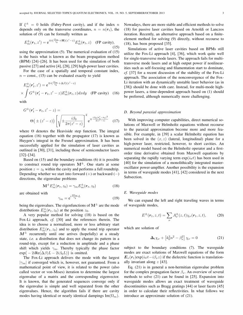
Fig. 1. Profiles of real part of refractive index(blue solid, left axis), intensity(red solid, right axis) and constant phase (red dotted, right axis) of the leakywaveguide under study. The real part of the effective index is also shown(blue dotted, left axis.)

F. Effective index method

For a nearly planar waveguide, i.e. if the mode profileχ(x, y) does not vary strongly along the x direction, (21) canbe solved perturbationally [46]. We choose

χ(x, y) = Φ(x, y)φ(x) (22)

where the dependence of Φ(x, y) on x is only parametrically.If Φ(x, y) is the solution of the eigenvalue problem

d2Φ

dy2+ k2

0

[n2 − n2

eff

]Φ = 0 (23)

with ∫ ∞−∞

Φ2dy = 1, (24)

then φ(x) obeys the eigenvalue problem

d2φ

dx2+[k2

0

(n2

eff + ∆n2eff

)− β2

]φ = 0 (25)

with∆n2

eff =

∫ [n2 − n2

]Φ2dy. (26)

In (23), n(x, y) is a typically real-valued chosen refractive-index distribution of a reference waveguide and neff(x) is theso-called effective index at position x. The correction ∆neffgiven by (26) could include e.g. modifications of the index dueto carrier density and temperature effects as well as the imag-inary part. The approach sketched above is called “effective-index method” in the semiconductor laser community. Eq. (23)is widely used in the design of high-power lasers, because itallows the optimization of the layer structure with respect tooptical confinement, far-field divergence and optical losses. Inwhat follows we will consider an example.

G. Worked example

Lasers grown on GaAs substrates, suffer from a leakage ofthe lasing mode into the substrate, or a coupling of the lasingmode with substrate modes because the refractive index ofthe substrate is typically larger than the effective index of thelasing mode. Although this effect is well-known for a long

0.1 0.2 0.3 0.4 0.5 0.6 0.7 0.8 0.9 1.0

0.01

0.1

1

10

100

= 1 µmdsub infinite

mod

al lo

ss [c

m-1

]

cladding thickness dcl [µm]

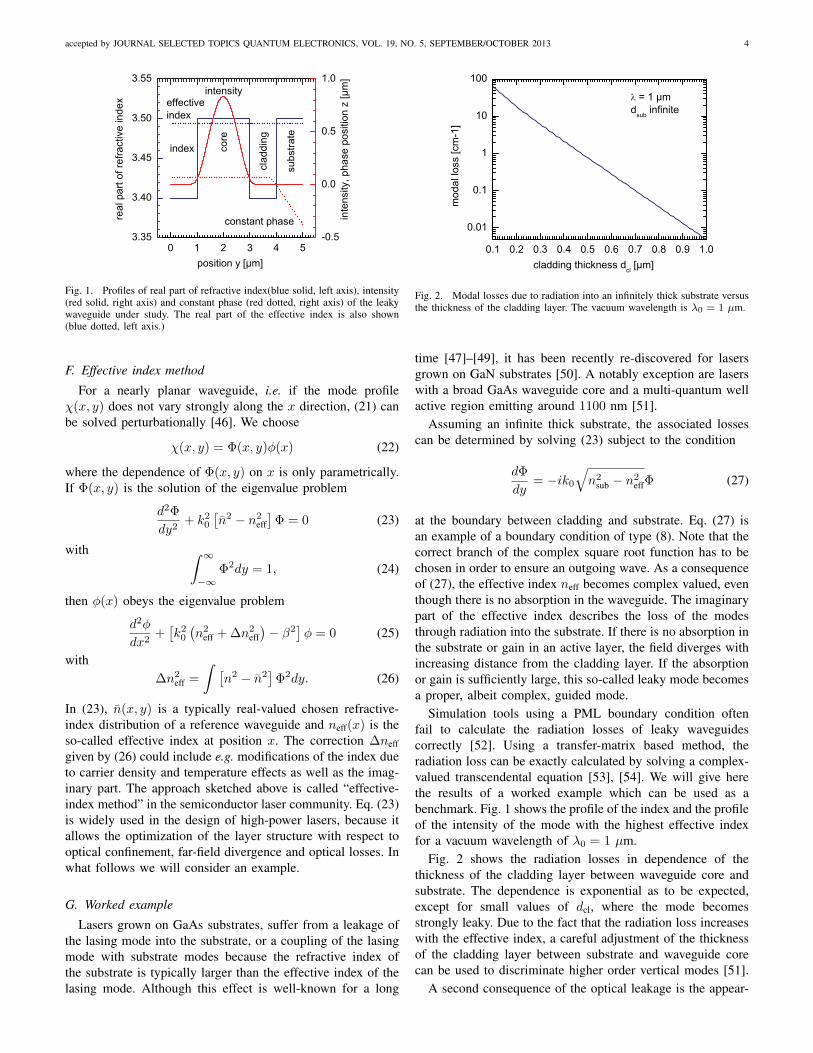
Fig. 2. Modal losses due to radiation into an infinitely thick substrate versusthe thickness of the cladding layer. The vacuum wavelength is λ0 = 1 µm.

time [47]–[49], it has been recently re-discovered for lasersgrown on GaN substrates [50]. A notably exception are laserswith a broad GaAs waveguide core and a multi-quantum wellactive region emitting around 1100 nm [51].

Assuming an infinite thick substrate, the associated lossescan be determined by solving (23) subject to the condition

dΦ

dy= −ik0

√n2

sub − n2effΦ (27)

at the boundary between cladding and substrate. Eq. (27) isan example of a boundary condition of type (8). Note that thecorrect branch of the complex square root function has to bechosen in order to ensure an outgoing wave. As a consequenceof (27), the effective index neff becomes complex valued, eventhough there is no absorption in the waveguide. The imaginarypart of the effective index describes the loss of the modesthrough radiation into the substrate. If there is no absorption inthe substrate or gain in an active layer, the field diverges withincreasing distance from the cladding layer. If the absorptionor gain is sufficiently large, this so-called leaky mode becomesa proper, albeit complex, guided mode.

Simulation tools using a PML boundary condition oftenfail to calculate the radiation losses of leaky waveguidescorrectly [52]. Using a transfer-matrix based method, theradiation loss can be exactly calculated by solving a complex-valued transcendental equation [53], [54]. We will give herethe results of a worked example which can be used as abenchmark. Fig. 1 shows the profile of the index and the profileof the intensity of the mode with the highest effective indexfor a vacuum wavelength of λ0 = 1 µm.

Fig. 2 shows the radiation losses in dependence of thethickness of the cladding layer between waveguide core andsubstrate. The dependence is exponential as to be expected,except for small values of dcl, where the mode becomesstrongly leaky. Due to the fact that the radiation loss increaseswith the effective index, a careful adjustment of the thicknessof the cladding layer between substrate and waveguide corecan be used to discriminate higher order vertical modes [51].

A second consequence of the optical leakage is the appear-


0.0

0.5

1.0 = 1 µm

rela

tive

inte

nsiti

ydsub infinitedcl = 1 µm

-50 0 500.0

0.5

1.0dsub = 120 µmdcl = 1 µm

angle [°]

Fig. 3. Vertical profiles of the far field intensities for a substrate infinitelythick (top) and with a finite thickness (bottom).

ance of additional peak(s) in the profile of the far field intensity

PFF (Θ) ∝ cos2(Θ)∣∣∣ ∫ Φ(y)eik0sin(Θ)ydy

∣∣∣2 (28)

in dependence on the vertical divergence angle Θ. If the modeprofile in the substrate

Φ(y) ∝ e−ik0

√n2

sub−n2effy (29)

is inserted into (28), there is a resonance if

sin2(Θr) = n2sub − n2

eff (30)

holds. Depending whether a substrate with an infinite (Fig.3, top) or finite (Fig. 3, bottom) thickness is assumed, oneresonance or two resonances, respectively, will be observed inthe far field profile. The magnitude and width of the peaksdepend on the absorption in the substrate and the bottomsurface roughness and metalization. The additional peak(s) inthe farfield can be observed if the condition 0 < n2

sub−n2eff < 1

holds. If n2sub − n2

eff > 1, the internal propagation angleΘi = acos(neff/nsub), which is the angle of the normal ofthe line of constant phase shown in Fig. 1 with respect to thez axis, is larger than the critical angle of total reflection andno peak appears.

A third consequence of the coupling of the lasing modewith substrate modes is a modulation of the intensity in thecenter of the waveguide core (or the optical confinementfactor) in dependence on the wavelength as shown in Fig.4. The modulation period depends strongly on the width ofthe waveguide core because the smaller the core the larger thewavelength dependence of the index of the mode confined tothe core. This effect results in a modulation of the modal gainand hence in a corresponding modulation of the spectrum ofthe amplified spontaneous emission [49], [55] and the opticalspectrum above threshold [56].

It should be noted that the GaAs p-contact layer causesmode coupling phenomena, too, if the thickness is not properlychosen [48].

0.95 1.00 1.050.0

0.5

1.0

dcore [ m] 0.5 1 2

rela

tive

inte

nsity

in c

ore

cent

er

wavelength [nm]

Fig. 4. Relative intensity in the waveguide core versus vacuum wavelengthfor different width of the waveguide core as indicated.

H. Longitudinal modes

If we insert (20) into (9) and neglect the coupling ofdifferent transverse modes due to a spatially varying groupindex, temporally varying index or spatially varying indexperturbations, the mode amplitudes obey

iΩνkvg,ν

A±νk ±dA±νkdz

+ i∆βνA±νk + iκ±ν A

∓νk = 0, (31)

with the abbreviation

∆βν =1

2β0

[β2ν − β2

0

]. (32)

For a Fabry-Perot laser, where the coupling coefficients

κ±ν =k2

0

∫ξ±E2

ν dxdy

2β0

∫E2ν dxdy

(33)

vanish, Eq. (31) can be analytically solved subject to theboundary conditions (6). From the complex mode frequenciesand (10) the wavelengths of the modes relative to the referencewavelength can be determined to

∆λFPνk = − λ2

0

2Lπng,ν

[ϕ0 + ϕL2

+ πk − Lβ0 − LRe(∆βν)]

(34)where k is the longitudinal mode index and ϕ0 and ϕLare the phases of the reflectivities. The spacing between thewavelengths of different transverse modes belonging to thesame longitudinal mode is approximately given by

λνk − λν′k ≈λ0

ng,ν(nmod,ν − nmod,ν′) (35)

with nmod,ν = Re(βν)/k0.Several cases can be distinguished depending on the differ-

ence of the modal indices governing the wavelength spacingof the transversal modes. For example, in a ridge waveguidelaser with a narrow ridge, the spacing of the wavelengths ofthe lateral modes is in the order of 1 nm which is muchlarger than that of the longitudinal modes. Hence, every lateralmode is associated with a comb of longitudinal modes whichcan overlap. In a broad-area laser with a wide ridge or gainregion, on the other hand, the spacing of the wavelengths ofthe lateral modes is typically much smaller than that of the


longitudinal modes, so that in a measured optical spectrumeach longitudinal mode splits into several peaks belonging tothe different lateral modes.

Assuming a 1D waveguide with width W and constant realrefractive index nr surrounded by perfect electric walls, themodal indices are

nmod,ν =

√n2

r −λ2

0

4W 2ν2 with ν = 1, 2, 3, · · · . (36)

Thus the wavelength spacing with respect to the fundamentalmode ν = 1 is given approximately

λνk − λ1k ≈λ3

0

8nrngW 2(1− ν2), (37)

which has been used by several authors [57], [58] for studiesof broad-area lasers. It should be noted that (37) is anapproximation, because it neglects the true profile of the indexand the penetration of the fields into the exterior region.

III. TIME-DEPENDENT ACTIVE CAVITY SIMULATION

A. Model equations

In order to assess the multi-mode behavior, modal instabil-ities and filamentation effects of wide-aperture semiconductorlasers a time-dependent approach is the most appropriate oneas outlined in Section II. Due to computer limitations, untilnow only the vertical-projected equations [59], [60]

− i

vg,eff

∂E±

∂t∓ i∂E

±

∂z+

1

2β0

∂2E±

∂x2

+k2

0

[n2

eff + ∆n2eff

]− β2

0

2β0E± +

k20κ±

2β0E∓ = Fspont (38)

with

κ± =k2

0

2β0

∫ξ±Φ2dy (39)

have been dealt with. They are obtained by introducing anAnsatz like (22) into (1) and adding a Langevin source Fsponton the rhs describing spontaneous emission. Dispersion of theimaginary part of the index (optical gain) must be additionallyincluded to eliminate the high-k instability [61], which canbe done on a microscopic level [62], [63], as an effectivepolarization [59] modeling a Lorentzian shape of the gain,with higher order time derivatives [64], by means of a digitalfilter [65], or by a convolution integral [66].

Eq. (38) has to be supplemented by equations governing thecarrier dynamics. In all models so far published this is done onthe level of a diffusion equation for the excess carrier densityN ,

∂N

∂t−∇

[D∇N

]+R(N) +Rstim =

j

ed(40)

assuming charge neutrality in the active region. The thick-ness of the active region is denoted by d and the ratesof spontaneous (including non-radiative and radiative) andstimulated recombination by R and Rstim, respectively, and∇ = (∂/∂x, ∂/∂z).

-5 0 50

10

20

30

40

50

60 w/o thermal lensing with thermal lensing

inte

nsity

[a.u

.]

lateral angle [degrees]

P = 7 W

Fig. 5. Time-averaged lateral profiles of the far field intensity of a gain-guidedBA DFB laser without and with the thermal lensing effect at an output powerof P = 7 W.

The current density is given by [67]

j(x, z) =

[U − UF(x, z)

]/r if x, z ∈ active stripe[

∇2UF]/Ω elsewhere

(41)with U being the bias and r and Ω being the resistivity andthe sheet resistance, respectively, of the p-doped layers. Thedependence of the current density within the active stripe onthe Fermi voltage UF, i.e. the spacing of the electro-chemicalpotentials of electrons and holes, results in a preferred currentinjection into regions with a low carrier density, thus coun-teracting spatial holeburning [68], [69]. The reason is thatUF decreases and thus the difference U − UF increases withdecreasing N .

As shown in [70], the diffusion coefficient reads

D = µp(p0 +N)dUF

dN(42)

with µp being the mobility of the holes in the active layerand p0 the equilibrium density of the holes. For Boltzmannstatistics, it is given by D = 2kBTµp/e (kB Boltzmannconstant, T temperature, e elementary charge).

The rate of stimulated recombination is given by

Rstim = vg,eff geff[|E+|2 + |E−|2

](43)

with the effective gain

geff =1

Re(neff)

∫nrgΦ2dy. (44)

The output power P0,L at z = 0 and z = L is then given by

P0,L = hω0vg,eff d(1− r20,L)

∫|E∓(x, z)|2z=0,Ldx. (45)

Note, that the dispersion of the gain must be included into(43), too.

B. Worked example

The multi-peaked and not diffraction-limited lateral fieldprofile of wide-aperture semiconductor lasers has been a longstanding problem and has been investigated in the past bynumerous authors [38], [71]–[74]. Although the broadening


wavelength [nm]

late

ral a

ngle

[de

gre

es]

spectrally resolved far field [dB]

969.6 969.7 969.8 969.9

-7

-6

-5

-4

-3

-2

-1

0

1

2

3

4

5

6

7-20

-10

0

10

20

30

40

50

60

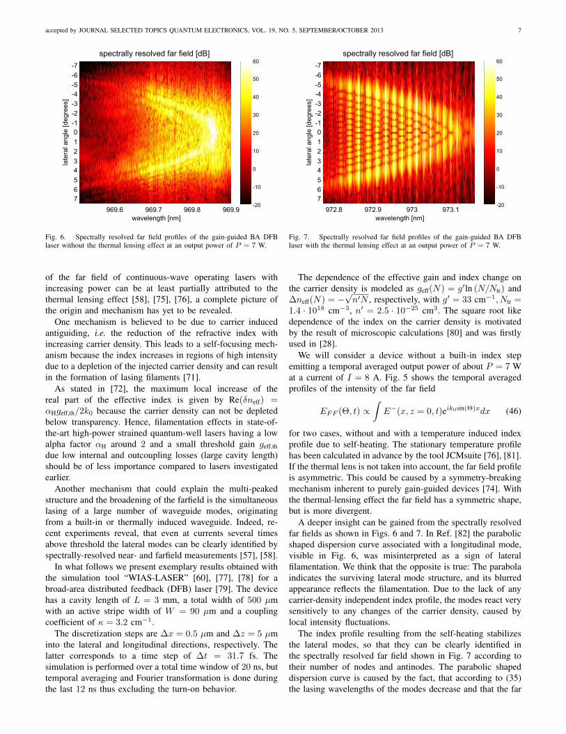
Fig. 6. Spectrally resolved far field profiles of the gain-guided BA DFBlaser without the thermal lensing effect at an output power of P = 7 W.

of the far field of continuous-wave operating lasers withincreasing power can be at least partially attributed to thethermal lensing effect [58], [75], [76], a complete picture ofthe origin and mechanism has yet to be revealed.

One mechanism is believed to be due to carrier inducedantiguiding, i.e. the reduction of the refractive index withincreasing carrier density. This leads to a self-focusing mech-anism because the index increases in regions of high intensitydue to a depletion of the injected carrier density and can resultin the formation of lasing filaments [71].

As stated in [72], the maximum local increase of thereal part of the effective index is given by Re(δneff) =αHgeff,th/2k0 because the carrier density can not be depletedbelow transparency. Hence, filamentation effects in state-of-the-art high-power strained quantum-well lasers having a lowalpha factor αH around 2 and a small threshold gain geff,thdue low internal and outcoupling losses (large cavity length)should be of less importance compared to lasers investigatedearlier.

Another mechanism that could explain the multi-peakedstructure and the broadening of the farfield is the simultaneouslasing of a large number of waveguide modes, originatingfrom a built-in or thermally induced waveguide. Indeed, re-cent experiments reveal, that even at currents several timesabove threshold the lateral modes can be clearly identified byspectrally-resolved near- and farfield measurements [57], [58].

In what follows we present exemplary results obtained withthe simulation tool “WIAS-LASER” [60], [77], [78] for abroad-area distributed feedback (DFB) laser [79]. The devicehas a cavity length of L = 3 mm, a total width of 500 µmwith an active stripe width of W = 90 µm and a couplingcoefficient of κ = 3.2 cm−1.

The discretization steps are ∆x = 0.5 µm and ∆z = 5 µminto the lateral and longitudinal directions, respectively. Thelatter corresponds to a time step of ∆t = 31.7 fs. Thesimulation is performed over a total time window of 20 ns, buttemporal averaging and Fourier transformation is done duringthe last 12 ns thus excluding the turn-on behavior.

wavelength [nm]

late

ral a

ngle

[de

gre

es]

spectrally resolved far field [dB]

972.8 972.9 973 973.1

-7

-6

-5

-4

-3

-2

-1

0

1

2

3

4

5

6

7-20

-10

0

10

20

30

40

50

60

Fig. 7. Spectrally resolved far field profiles of the gain-guided BA DFBlaser with the thermal lensing effect at an output power of P = 7 W.

The dependence of the effective gain and index change onthe carrier density is modeled as geff(N) = g′ln (N/Ntr) and∆neff(N) = −

√n′N , respectively, with g′ = 33 cm−1, Ntr =

1.4 · 1018 cm−3, n′ = 2.5 · 10−25 cm3. The square root likedependence of the index on the carrier density is motivatedby the result of microscopic calculations [80] and was firstlyused in [28].

We will consider a device without a built-in index stepemitting a temporal averaged output power of about P = 7 Wat a current of I = 8 A. Fig. 5 shows the temporal averagedprofiles of the intensity of the far field

EFF (Θ, t) ∝∫E−(x, z = 0, t)eik0sin(Θ)xdx (46)

for two cases, without and with a temperature induced indexprofile due to self-heating. The stationary temperature profilehas been calculated in advance by the tool JCMsuite [76], [81].If the thermal lens is not taken into account, the far field profileis asymmetric. This could be caused by a symmetry-breakingmechanism inherent to purely gain-guided devices [74]. Withthe thermal-lensing effect the far field has a symmetric shape,but is more divergent.

A deeper insight can be gained from the spectrally resolvedfar fields as shown in Figs. 6 and 7. In Ref. [82] the parabolicshaped dispersion curve associated with a longitudinal mode,visible in Fig. 6, was misinterpreted as a sign of lateralfilamentation. We think that the opposite is true: The parabolaindicates the surviving lateral mode structure, and its blurredappearance reflects the filamentation. Due to the lack of anycarrier-density independent index profile, the modes react verysensitively to any changes of the carrier density, caused bylocal intensity fluctuations.

The index profile resulting from the self-heating stabilizesthe lateral modes, so that they can be clearly identified inthe spectrally resolved far field shown in Fig. 7 according totheir number of nodes and antinodes. The parabolic shapeddispersion curve is caused by the fact, that according to (35)the lasing wavelengths of the modes decrease and that the far


time [ns]

late

ral coord

inate

[µ

m]

time-resolved near field intensity [W/µm2]

0 0.5 1 1.5 2

-100

-50

0

50

100 0

5

10

15

20

25

30

35

40

Fig. 8. Time-resolved near field profiles of the gain-guided BA DFB laserwithout the thermal lensing effect at an output power of P = 7 W.

field divergence increases with rising mode index. A similarinterpretation was also given in [83]. We should note, thatthere is only one longitudinal mode lasing due to the DFBoperation.

The time-resolved near fields shown in Figs. 8 and 9 revealthe non-stationary behavior, which was already found earlier[84]. It can be interpreted to be caused by mode beating intime and space. Obviously, in the purely gain-guided case(Fig. 8) less modes are involved compared to the case witha superimposed index profile (Fig. 9). The appearance of thebright spots can be thought to be the result of a constructiveinterference of the lateral modes. Although the results areencouraging, further analytical and numerical investigationsare needed in order to reveal the relative contributions oflateral mode and filamentary structures to the optical field ofwide-aperture lasers and to obtain quantitative agreement withexperimental results.

IV. STATIONARY DRIFT-DIFFUSION BASED SIMULATION

A. Basic equations

The standard model [85]–[87] for the numerical evaluationof the distributions of the electron and hole densities N andP , temperature T and electron and hole densities jn and jpin semiconductor lasers is the energy transport model, whichconsist of the Poisson equation for the electro-static potentialϕ,

−∇[εs∇ϕ

]= C − P +N (47)

with εs being the static dielectric constant and C the chargedimpurity density, the continuity equations

∇jn = R+Rstim (48)−∇jp = R+Rstim (49)

and the heat flow equation

−∇[κL∇T

]= H (50)

with κL being the thermal conductivity. The various implemen-tations of the model differ in the assumptions for the current

time [ns]

late

ral coord

inate

[µ

m]

time-resolved near field intensity [W/µm2]

0 0.5 1 1.5 2

-100

-50

0

50

100 0

5

10

15

20

25

30

35

40

45

50

Fig. 9. Time-resolved near field profiles of the gain-guided BA DFB laserwith the thermal lensing effect at an output power of P = 7 W.

densities the jn, jp and the heat source H . Expressions inagreement with the thermodynamic principles can be found inRef. [88]. The rate of stimulated recombination is given hereby

Rstim =nrg

hω0

∑ν

Pν |χν |2

nmod,ν∫|χν |2dxdy

(51)

with χν obtained by solving (21).The equations are supplemented by proper boundary condi-

tions [88]. For example, the boundary condition for the heatflow equation reads

νκL∇T = h[Ts − T

](52)

where ν is the normal unit vector and Ts is the heat sinktemperature. The heat transfer coefficient h models the heatflow to the exterior region.

The optical output power for a given applied bias U isobtained by a solution of (31). However, in Fabry-Perotlasers it is sufficient to determine the forward and backwardpropagating optical power P+

ν = |A+ν |2 and P−ν = |A−ν |2,

which are solutions of the equations

± dP±νdz

=

[2Im

(βν +

Ωνvg,ν

)− α0

]P±ν (53)

with Pν = P+ν + P−ν . The loss coefficient α0 includes all

loss mechanisms which are not already accounted for in theimaginary part of β, such as additional internal or scatteringlosses. The equations (53) have to be solved subject to theboundary conditions

P+ν (0) = R0P

−ν (0) and P−ν (L) = RLP

+ν (L). (54)

The lasing wavelength can be approximately determinedby determining the maximum of the integral

∫ L0

Im(βν +

Ων/vg,ν)dz.

Eqs. (31) or (53) can be conveniently solved by the “TreatPower as a Parameter” (TPP) method as introduced in [68]and used in [89]. It is based on the observation, that therelative propagation factor ∆βν in (31) or imaginary partIm(βν) in (53) can be considered to be a function of the


0 10 200

5

10

15

20

25

optic

al p

ower

[W]

injection current [A]

0.0

0.1

0.2

0.3

0.4

0.5

0.6

0.7

0.8

0.9

1.0

simulation w/o LSH simulation with LSH experiment

conv

ersi

on e

ffici

ency

= 915nmL = 6 mmW= 95 µmT = 25°C

Fig. 10. Measured (solid red) and simulated optical output power (left axis)and conversion efficiency (right axis) versus injection current. The simulationswere done without (dashed blue) and with (solid green) longitudinal spatialholeburning.

bias, the local power and the unknown wavelengths of thelasing and nonlasing modes. Thus, in a first step one calculates∆βν as a function of U , the power of the lasing waveguidemode Pνl = P+

νl+ P−νl , and the wavelengths by solving the

drift-diffusion and waveguide equations in the transverse crosssection and stores the results in a in a look-up table. In asecond step, (53) is solved by interpolating in the look-uptable. For the lasing waveguide mode, Im(Ωνl) has to vanishand one has to determine the output power and the wavelengthfor given U . For the non-lasing waveguide modes one has todetermine Ων for the given U and the power distribution ofthe lasing mode.

Longitudinal spatial hole burning (LSH) is included auto-matically via the power dependence of Im(βν) in Eq. (53). IfIm(βν) is evaluated at the average power Pνl =

∫ [P+νl

+P−νl]dz/L in the cavity, the usual model neglecting LSH

is recovered, because (53) is linear and can be analyticallysolved.

B. Worked example

In what follows we present results obtained with the sim-ulation tool “WIAS-TeSCA” [90] for a broad-area laser. Thedevice with a cavity length of L = 6 mm and an active stripewidth of W = 95 µm has a double quantum well (DQW)InGaAs/GaAsP active region embedded into 2.2 µm wideAl0.30Ga0.70As confinement and Al0.85Ga0.15As cladding lay-ers. The optical confinement factor of the DQW totals 1.8%.We performed a one-dimensional simulation in the transversecross section neglecting any lateral effects as outlined in [91]and [92]. The pre-factor for the gain and the Shockley-Read-Hall recombination life times ( τn = τp = 1.3 ns identicalfor all layers) have been fitted on the results of length-dependent pulsed measurements of threshold current and slopeefficiency of uncoated devices. The cross-sections of free-carrier absorption have been chosen to fcn = 3 × 10−18 cm2

0

5

10

15

20

25

0 1 2 3 4 5 60

5

10

15 w/o LSH with LSH

opt

ical

pow

er [W

] m

odal

gai

n [c

m-1]

longitudinal position z [mm]

Fig. 11. Longitudinal profiles of optical power (top) and modal gain (bottom)at an injection current of I = 25 A without (dashed blue) and with (solidgreen) longitudinal spatial holeburning.

and fcp = 7×10−18 cm2 for electrons and holes, respectively.Fig. 10 shows the measured and simulated power-current

characteristics of the laser. Experimentally, a maximum outputpower of P = 20 W at a current of I = 25 A wasachieved limited by thermal rollover. The experimental datawere reproduced theoretically in a two-stage process with andwithout LSH. The reason for the rollover of the characteristicsoccurring already without LSH has been explained in detailin [92]. With increasing current and power, the reduction ofthe gain caused by the temperature rise (∆T = 42 K atI = 25 A) must be compensated for by a correspondingincrease in the carrier densities in the active region, whichleads as a consequence also to an increase in the carrierdensities in the confinement layers. Another effect is thebending of the quasi-Fermi energy of the holes with increasingapplied bias and, as a consequence, the bending of the band-edge energies due to the voltage drop in the p-doped layers.This leads to a corresponding linear increase in the electrondensity with increasing distance from the active region up ton ≈ 3 × 1016 cm−3. The increased carrier densities in theactive region and in the bulk layers give rise to enhancednon-stimulated recombination and free-carrier absorption [93],[94].

However neglecting LSH, not only the roll-over power, butalso the conversion efficiency is exaggerated which is dueto the overestimation of the slope-efficiency. Good agreementbetween measurement and simulation is only achieved if LSHis included, as Fig. 10 reveals.

To illustrate the mechanism of LSH, Fig. 11 shows thelongitudinal profiles of the optical power, the modal gain andthe injected current density for the two models at a current ofI = 25 A. The rear facet with a reflectivity of RL = 0.98 islocated at z= 6 mm and the front facet with a reflectivity ofR0 = 0.005 at z = 0. LSH leads to a strong depletion of thegain in the vicinity of the front facet, which is compensated bya corresponding rise of the gain at the rear facet. This results


in a weaker increase of the power towards the front facet andhence a lower power at z = 0, i.e. a lower output power, andis in contrast to Ref. [95] where based on an analytical modelit was found that the values of the power at the facets don’tdependent on the fact, whether LSH is considered or not.

It should be noted, that even with LSH there is still a smalldeviation in roll-over power and conversion efficiency betweenmeasurement and simulation. One reason is the neglect of theseries resistances of the p-contact and the substrate in the sim-ulation, which lead to an additional voltage drop reducing theconversion efficiency but also to additional heating reducingthe roll-over power.

C. Heterojunctions

Heterojunctions characterized by discontinuities in theedges of the conduction and valance bands as well as abruptchanges of effective masses and mobilities require specialattention. If the validity of the thermodynamic based drift-diffusion approach is assumed, the electro-chemical potentialsshould be continuous through the heterojunctions. The rea-son is, that the electro-chemical potentials and the inversetemperature can be interpreted as Lagrange multipliers in thefunctional for the maximization of the entropy subject to theconstraints of charge and energy conservation [96].

The widely used thermionic emission theory which es-tablishes additional conditions for the current densities [97],[98] is restricted to situations where the current essentiallyflows perpendicular to the junction and cannot be appliedto intersections of three or more materials [99]. In high-power lasers there is no need to apply the thermionic emissiontheory with its difficulties because typically all heterojunctions(except at the QWs) are graded in order to avoid any drops ofthe electro-static potential.

D. Quantum effects

In the simulations presented in subsection IV-B, the carriersin all layers were treated within the drift-diffusion approach,neglecting quantum effects. For more accurate simulationselectrons and holes confined in active QWs must be treatedin a special manner. As outlined in detail in [87], [99]–[102],the transport of the confined carriers in the in-plane directions(x, z) can be described by classical drift-diffusion, but in theperpendicular direction y the carriers have to be described bytheir quantum-mechanical wave functions. Therefore, the car-riers population partitions into carriers which have sufficientenergy to be be considered as unconfined and those which areconfined. The scattering between both populations is describedby a capture rate which has to be included into the continuityequations (48) as a recombination rate for the unconfined anda generation rate for the confined carriers.

It should be noted that the statistics of both carrier pop-ulations is governed by different electro-chemical potentials.Whereas the quasi-chemical potentials of the unconfined car-riers depend directly on the bias applied to the contacts,the quasi-chemical potentials of the unconfined carriers aredetermined by the capture rates. Coupling of the populationstakes also place via the Poisson equation (47).

Although the sketched picture where carriers are describedquantum-mechanically in one direction and classically in theothers has been included in several simulation tools, thereare still open questions which have to be solved. The energywhich partitions the carrier populations can not be alwaysclearly defined, for example in the case of a QW located inan unbiased pn-junction. Another issue is the correct treatmentof the transport in multi-quantum well structures between theQWs through the barriers.

The impact of the non-equilibrium between confined andunconfined carriers in high-power lasers on the internal effi-ciency, e.g., has been investigated until now using only rate-equation approaches [103], not the drift-diffusion model.

V. SUMMARY AND OUTLOOK

We presented models for the calculation of passive cavitymodes, for the investigation of the spatiotemporal behavior ofthe optical field and of the stationary simulation of the light-current characteristics of high-power semiconductor lasers.Future work should be directed at full three-dimensionalcalculation of the optical field and an improvement of thephysical models underlying the time-dependent active cavitysimulations, including a better description of the carrier andheat transport by the energy transport model instead of thediffusion equation and stationary heat conduction equation.Finally, we would like to mention that the dependence ofmany material parameters and functions such as mobilitiesand absorption coefficients on composition, temperature anddoping is not well known and needs to be improved.

APPENDIXPROOF OF MODE ORTHOGONALITY

Let us write down (1) for 2 modes with indices m and m′:[k0nngΩmcβ0

− i ∂∂z

+1

2β0∆t + ∆β

]E+m +

k20ξ

+

2β0E−m = 0

(55)[k0nngΩmcβ0

+ i∂

∂z+

1

2β0∆t + ∆β

]E−m +

k20ξ−

2β0E+m = 0

(56)[k0nngΩm′

cβ0− i ∂

∂z+

1

2β0∆t + ∆β

]E+m′ +

k20ξ

+

2β0E−m′ = 0

(57)[k0nngΩm′

cβ0+ i

∂

∂z+

1

2β0∆t + ∆β

]E−m′ +

k20ξ−

2β0E+m′ = 0

(58)Next (55) is multiplied with E−m′ , (56) with E+

m′ , (57) with−E−m, and (58) with −E+

m. Then all equations are integratedover the cavity and added to obtain

k0 (Ωm − Ωm′)

cβ0

∫nng

[E+mE−m′ + E−mE

+m′

]dxdydz

− i∫

∂

∂z

[E+mE−m′ − E

−mE

+m′

]dxdydz

+1

2β0

∫∇t[E−m′∇tE

+m + E+

m′∇tE−m

− E−m∇tE+m′ − E

+m∇tE−m′

]dxdydz = 0 (59)


where the derivatives have been factored out. The second andthird terms vanishes due to the boundary conditions (6)-(7).Hence, the first term has to vanish, too, with leads to (11).

ACKNOWLEDGMENT

The author would like to thank R. Guther and P. Crump(FBH) for a critical reading of the manuscript and M. Radz-iunas and U. Bandelow (WIAS) for providing the simulationtool “WIAS-LASER”.

REFERENCES

[1] D. Welch, “A brief history of high-power semiconductor lasers,” IEEEJ. Sel. Topics Quantum Electron., vol. 6, no. 6, pp. 1470–1477, 2000.

[2] R. Diehl, High-power Diode Lasers: Fundamentals, Technology, Ap-plications. Berlin Heidelberg New York: Springer, 2000, vol. 78.

[3] M. Behringer, “High-power diode laser technology and characteristics,”in High Power Diode Lasers, ser. Springer Series in Optical Sciences,F. Bachmann, P. Loosen, and R. Poprawe, Eds. New York: Springer,2007, vol. 128, pp. 5–74.

[4] J. J. Lim, S. Sujecki, L. Lang, Z. Zhang, D. Paboeuf, G. Pauliat,G. Lucas-Leclin, P. Georges, R. C. I. MacKenzie, P. Bream, S. Bull, K.-H. Hasler, B. Sumpf, H. Wenzel, G. Erbert, B. Thestrup, P. M. Petersen,N. Michel, M. Krakowski, and E. C. Larkins, “Design and simulationof next-generation high-power, high-brightness laser diodes,” IEEE J.Sel. Topics Quantum Electron., vol. 15, no. 3, pp. 993–1008, May-Jum2009.

[5] H. Weber, P. Loosen, and R. Poprawe, Eds., Laser Physics andApplications, Subvolume B: Laser Systems, ser. Landolt Bornstein.Berlin Heidelberg New York: Springer, 2011, vol. 3.

[6] P. Crump, O. Brox, F. Bugge, J. Fricke, C. Schultz, M. Spreemann,B. Sumpf, H. Wenzel, and G. Erbert, “High-power, high-efficiencymonolithic edge-emitting GaAs based lasers with narrow spectralwidths,” in Advances in Semiconductor Lasers, ser. Semiconductorand Semimetals, J. J. Colemann, A. C. Bryce, and C. Jagadish, Eds.Amsterdam: Elsevier, 2012, vol. 86, ch. 2.

[7] A. E. Siegman, Lasers. Mill Valley: Univ. Science Books, 1986.[8] X. Antoine, A. Arnold, C. Besse, M. Ehrhardt, and A. Schadle, “A

review of transparent and artificial boundary conditions techniques forlinear and nonlinear Schrodinger equations,” Communic. Comp. Phys.,vol. 4, no. 4, pp. 729–796, Oct 2008.

[9] T. Moore, J. Blaschak, A. Taflove, and G. Kriegsmann, “Theory andapplication of radiation boundary operators,” IEEE Trans. AntennasPropag., vol. 36, no. 12, pp. 1797–1812, 1988.

[10] A. Oskooi, L. Zhang, Y. Avniel, and S. Johnson, “The failure ofperfectly matched layers, and towards their redemption by adiabaticabsorbers,” Optics Express, vol. 16, no. 15, pp. 11 376–11 392, 2008.

[11] T. Tischler, Die Perfectly-Matched-Layer-Randbedingung in der Finite-Differenzen-Methode im Frequenzbereich: Implementierung und Ein-satzbereiche, ser. Innovationen mit Mikrowellen und Licht. Cuvillier,2004.

[12] H. Wenzel and H.-J. Wunsche, “An equation for the amplitudes of themodes in semiconductor lasers,” IEEE J. Quantum Electron., vol. 30,no. 9, pp. 2073–2080, Sep 1994.

[13] D. V. Batrak and A. P. Bogatov, “Approximate orthogonality relationfor the modes of an open cavity,” Quantum Electronics, vol. 35, no. 4,pp. 356–358, Apr 2005.

[14] H. Wenzel, U. Bandelow, H.-J. Wunsche, and J. Rehberg, “Mechanismsof fast self pulsations in two-section DFB lasers,” IEEE J. QuantumElectron., vol. 32, no. 1, pp. 69–78, Jan 1996.

[15] W. D. Heiss, “Exceptional points of non-hermitian operators,” J. Phys.A: Math. Gen., vol. 37, no. 6, pp. 2455–2464, Feb 2004.

[16] M. V. Berry, “Mode degeneracies and the Petermann excess-noisefactor for unstable lasers,” J. Mod. Optics, vol. 50, no. 1, pp. 63–81,2003.

[17] H.-J. Wunsche, U. Bandelow, H. Wenzel, and D. D. Marcenac, “Selfpulsations by mode degeneracy in two-section DFB lasers,” Proc. SPIE,vol. 2399, pp. 195–206, 1995.

[18] M. Liertzer, L. Ge, A. Cerjan, A. D. Stone, H. E. Tuereci, and S. Rotter,“Pump-induced exceptional points in lasers,” Phys. Rev. Lett., vol. 108,no. 17, Apr 2012.

[19] J. Ctyroky, V. Kuzmiak, and S. Eyderman, “Waveguide structures withantisymmetric gain/loss profile,” Optics Express, vol. 18, no. 21, pp.21 585–21 593, Oct 2010.

[20] J. Rehberg, H.-J. Wunsche, U. Bandelow, and H. Wenzel, “Spectralproperties of a system describing fast pulsating DFB lasers,” Z. Angew.Math. Mech., vol. 77, no. 1, pp. 75–77, 1997.

[21] K. Petermann, Laser Diode Modulation and Noise. Dortrecht: KluwerAcademic, 1988.

[22] A. E. Siegman, “Lasers without photons - or should it be lasers with toomany photons,” Appl. Phys. B, vol. 60, no. 2-3, pp. 247–257, Feb-Mar1995.

[23] U. Bandelow, R. Schatz, and H.-J. Wunsche, “A correct single-modephoton rate equation for multisection lasers,” IEEE Photon. Technol.Lett., vol. 8, no. 5, pp. 614–616, May 1996.

[24] R. Marz, Integrated optics: Design and Modeling. Norwood, MA:Artech House, 1995.

[25] R. Scarmozzino, A. Gopinath, R. Pregla, and S. Helfert, “Numericaltechniques for modeling guided-wave photonic devices,” IEEE J. Sel.Topics Quantum Electron., vol. 6, no. 1, pp. 150–162, Jan-Feb 2000.

[26] T. Benson, B. B. Hu, A. Vukovic, and P. Sewell, “What is the futurefor beam propagation methods?” Proc. SPIE, vol. 5579, pp. 351–358,2004.

[27] S. Sujecki, J. Wykes, P. Sewell, A. Vukovic, T. M. Benson, E. C.Larkins, L. Borruel, and I. Esquivias, “Optical properties of taperedlaser cavities,” IEE Proc. Optoelectron., vol. 150, no. 3, pp. 246–252,Jun 2003.

[28] L. Borruel, S. Sujecki, P. Moreno, J. Wykes, M. Krakowski, B. Sumpf,P. Sewell, S. Auzanneau, H. Wenzel, D. Rodrıguez et al., “Quasi-3-D simulation of high-brightness tapered lasers,” IEEE J. QuantumElectron., vol. 40, no. 5, pp. 463–472, 2004.

[29] H. Odriozola, J. Tijero, L. Borruel, I. Esquivias, H. Wenzel, F. Dittmar,K. Paschke, B. Sumpf, and G. Erbert, “Beam properties of 980-nmtapered lasers with separate contacts: Experiments and simulations,”IEEE J. Quantum Electron., vol. 45, no. 1, pp. 42–50, 2009.

[30] A. E. Siegman, “Laser beams and resonators: The 1960s,” IEEE J.Sel. Topics Quantum Electron., vol. 6, no. 6, pp. 1380–1388, Nov-Dec2000.

[31] ——, “Laser beams and resonators: Beyond the 1960s,” IEEE J. Sel.Topics Quantum Electron., vol. 6, no. 6, pp. 1389–1399, Nov-Dec 2000.

[32] T. Fukushima, S. A. Biellak, Y. Sun, and A. E. Siegman, “Beampropagation behavior in a quasi-stadium laser diode,” Optics Express,vol. 2, no. 2, pp. 21–28, Jan 1998.

[33] M. Spreemann, H. Wenzel, B. Eppich, M. Lichtner, and G. Erbert,“Novel approach to finite-aperture tapered unstable resonator lasers,”IEEE J. Quantum Electron., vol. 47, no. 1, pp. 117–125, Jan 2011.

[34] M. Spreemann, J. Fricke, H. Wenzel, and G. Erbert, “Experimental andtheoretical study of finite-aperture tapered unstable resonator lasers,”Semicond. Sci. Technol., vol. 27, no. 10, Oct 2012.

[35] K. Altmann, C. Pflaum, and D. Seider, “Third-dimensional finiteelement computation of laser cavity eigenmodes,” Appl. Optics, vol. 43,no. 9, pp. 1892–1901, Mar 2004.

[36] A. P. Napartovich, N. N. Elkin, V. N. Troshchieva, D. V. Vysotsky, L. J.Mawst, and D. Botez, “Comprehensive analysis of mode competitionin high-power cw-operating diode lasers of the antiresonant reflectingoptical waveguide (ARROW) type,” IEEE J. Sel. Topics QuantumElectron., vol. 17, no. 6, pp. 1735–1744, Nov-Dec 2011.

[37] S. Sujecki, “Stability of steady-state high-power semiconductor lasermodels,” J. Opt. Soc. Am. B, vol. 24, no. 5, pp. 1053–1060, May 2007.

[38] J. Marciante and G. Agrawal, “Nonlinear mechanisms of filamentationin broad-area semiconductor lasers,” IEEE J. Quantum Electron.,vol. 32, no. 4, pp. 590–596, 1996.

[39] V. P. Kalosha, K. Posilovic, and D. Bimberg, “Lateral-longitudinalmodes of high-power inhomogeneous waveguide lasers,” IEEE J.Quantum Electron., vol. 48, no. 2, pp. 123–128, Feb 2012.

[40] B. Berneker and C. Pflaum, “Two-dimensional dynamic simulations ofDFB lasers and MOPAs,” Opt. Quantum Electron., vol. 41, no. 11-13,pp. 895–902, Nov 2009.

[41] R. Hocke and M. Marz, “Ein Berechnungsverfahren fur optisch insta-bile Wellenleiter-Resonatoren,” Frequenz, vol. 49, pp. 100–104, 1995.

[42] P. Bienstman, “Rigorous and efficient modelling of wavelength scalephotonic components,” Ph.D. dissertation, Univ. of Gent, 2001.

[43] J. Pomplun, S. Burger, F. Schmidt, A. Schliwa, D. Bimberg,A. Pietrzak, H. Wenzel, and G. Erbert, “Finite element simulation ofthe optical modes of semiconductor lasers,” Phys. Stat. Sol. B, vol. 247,no. 4, pp. 846–853, Apr 2010.

[44] J. Fricke, W. John, A. Klehr, P. Ressel, L. Weixelbaum, H. Wenzel,and G. Erbert, “Properties and fabrication of high-order Bragg gratingsfor wavelength stabilization of diode lasers,” Semicond. Sci. Technol.,vol. 27, no. 5, p. 055009, 2012.


[45] H. Derudder, D. De Zutter, and F. Olyslager, “Analysis of waveguidediscontinuities using perfectly matched layers,” Electron. Lett., vol. 34,no. 22, pp. 2138–2140, 1998.

[46] T. Kato, Perturbation Theory for Linear Operators. Berlin: Springer,1995.

[47] E. V. Arzhanov, A. P. Bogatov, V. P. Konyaev, O. M. Nikitina, and V. I.Shveikin, “Wave-guide properties of heterolasers based on quantum-well strained structures in InGaAs/GaAs system and characteristicproperties of their gain spectra,” Kvantovaya Elektronika, vol. 21, no. 7,pp. 633–639, Jul 1994.

[48] P. G. Eliseev and A. E. Drakin, “Analysis of the mode internal couplingin InGaAs/GaAs laser-diodes,” Laser Physics, vol. 4, no. 3, pp. 485–492, May-Jun 1994.

[49] I. A. Avrutsky, R. Gordon, R. Clayton, and J. M. Xu, “Investigations ofthe spectral characteristics of 980-nm InGaAs-GaAs-AlGaAs lasers,”IEEE J. Quantum Electron., vol. 33, no. 10, pp. 1801–1809, Oct 1997.

[50] V. Laino, F. Roemer, B. Witzigmann, C. Lauterbach, U. T. Schwarz,C. Rumbolz, M. O. Schillgalies, M. Furitsch, A. Lell, and V. Haerle,“Substrate modes of (Al,In)GaN semiconductor laser diodes on SiCand GaN substrates,” IEEE J. Quantum Electron., vol. 43, no. 1, pp.16–24, Jan-Feb 2007.

[51] G. Erbert, F. Bugge, J. Fricke, P. Ressel, R. Staske, B. Sumpf,H. Wenzel, M. Weyers, and G. Trankle, “High power high-efficiency1150-nm quantum-well laser,” IEEE J. Sel. Topics Quantum Electron.,vol. 11, no. 5, pp. 1217–1222, Sep-Oct 2005.

[52] P. Bienstman, S. Selleri, L. Rosa, H. P. Uranus, W. C. L. Hopman,R. Costa, A. Melloni, L. C. Andreani, J. P. Hugonin, P. Lalanne,D. Pinto, S. S. A. Obayya, M. Dems, and K. Panajotov, “Modellingleaky photonic wires: A mode solver comparison,” Opt. QuantumElectron., vol. 38, no. 9-11, pp. 731–759, Jul 2006.

[53] H. Wenzel and H. Wunsche, “A model for the calculation of thethreshold current of SCH-MQW-SAS lasers,” phys. stat. sol. (a), vol.120, no. 2, pp. 661–673, 1990.

[54] J. Petracek and K. Singh, “Determination of leaky modes in planarmultilayer waveguides,” IEEE Photon. Technol. Lett., vol. 14, no. 6,pp. 810–812, 2002.

[55] B. Witzigmann, V. Laino, F. Roemer, C. Lauterbach, U. T. Schwarz,C. Rumbolz, M. O. Schillgalies, A. Lell, U. Strauss, and V. Hrle,“Analysis of substrate modes in GaN/InGaN lasers,” Proc. SPIE, vol.6468, pp. 64 680Q–64 680Q–8, 2007.

[56] H. Horie, N. Arai, Y. Yamamoto, and S. Nagao, “Longitudinal-modecharacteristics of weakly index-guided buried-stripe type 980-nm laserdiodes with and without substrate-mode-induced phenomena,” IEEE J.Quantum Electron., vol. 36, no. 12, pp. 1454–1461, 2000.

[57] N. Stelmakh and M. Flowers, “Measurement of spatial modes of broad-area diode lasers with 1-GHz resolution grating spectrometer,” IEEEPhoton. Technol. Lett., vol. 18, no. 15, pp. 1618–1620, 2006.

[58] P. Crump, S. Boldicke, C. Schultz, H. Ekhteraei, H. Wenzel, andG. Erbert, “Experimental and theoretical analysis of the dominantlateral waveguiding mechanism in 975 nm high power broad area diodelasers,” Semicond. Sci. Technol., vol. 27, no. 4, p. 045001, 2012.

[59] C. Z. Ning, R. A. Indik, and J. V. Moloney, “Effective Bloch equationsfor semiconductor lasers and amplifiers,” IEEE J. Quantum Electron.,vol. 33, no. 9, pp. 1543–1550, Sep 1997.

[60] M. Lichtner, M. Radziunas, U. Bandelow, M. Spreemann, and H. Wen-zel, “Dynamic simulation of high brightness semiconductor lasers,”Proc. NUSOD ’08, pp. 65–66, 2008.

[61] P. K. Jakobsen, J. V. Moloney, A. C. Newell, and R. Indik, “Space-timedynamics of wide-gain-section lasers,” Phys. Rev. A, vol. 45, no. 11,p. 8129, 1992.

[62] C. Z. Ning, R. A. Indik, J. V. Moloney, W. W. Chow, A. Girndt,S. W. Koch, and R. H. Binder, “Incorporating many-body effects intomodeling of semiconductor lasers and amplifiers,” Proc. SPIE, vol.2994, pp. 666–677, 1997.

[63] E. Gehrig and O. Hess, “Spatio-temporal dynamics of light ampli-fication and amplified spontaneous emission in high-power taperedsemiconductor laser amplifiers,” IEEE J. Quantum Electron., vol. 37,no. 10, pp. 1345–1355, Oct 2001.

[64] S. Balsamo, F. Sartori, and I. Montrosset, “Dynamic beam propagationmethod for flared semiconductor power amplifiers,” IEEE J. QuantumElectron., vol. 2, no. 2, pp. 378–384, Jun 1996.

[65] M. Kolesik and J. V. Moloney, “A spatial digital filter method for broad-band simulation of semiconductor lasers,” IEEE J. Quantum Electron.,vol. 37, no. 7, pp. 936–944, Jul 2001.

[66] J. Javaloyes and S. Balle, “Quasiequilibrium time-domain susceptibilityof semiconductor quantum wells,” Phys. Rev. A, vol. 81, no. 6, p.062505, 2010.

[67] W. Joyce, “Current-crowded carrier confinement in double-hetero-structure lasers,” J. Appl. Phys., vol. 51, no. 5, pp. 2394–2401, 1980.

[68] H. Wunsche, U. Bandelow, and H. Wenzel, “Calculation of combinedlateral and longitudinal spatial hole burning in λ/4 shifted DFB lasers,”IEEE J. Quantum Electron., vol. 17, pp. 1751–1760, 1993.

[69] P. Eliseev, A. Glebov, and M. Osinski, “Current self-distribution effectin diode lasers: analytic criterion and numerical study,” IEEE J. Sel.Topics Quantum Electron., vol. 3, no. 2, pp. 499–506, 1997.

[70] W. Joyce, “Carrier transport in double-heterostructure active layers,” J.Appl. Phys., vol. 53, no. 11, pp. 7235–7239, 1982.

[71] G. H. B. Thompson, “A theory for filamentation in semiconductorlasers including the dependence of dielectric constant on injectedcarrier density,” Opto-electronics, vol. 4, pp. 257–310, 1972.

[72] D. Mehuys, R. Lang, M. Mittelstein, J. Salzman, and A. Yariv, “Self-stabilized nonlinear lateral modes of broad area lasers,” IEEE J.Quantum Electron., vol. 23, no. 11, pp. 1909–1920, 1987.

[73] R. Lang, A. Larsson, and J. Cody, “Lateral modes of broad areasemiconductor lasers: Theory and experiment,” IEEE J. QuantumElectron., vol. 27, no. 3, pp. 312–320, 1991.

[74] S. Blaaberg, P. Petersen, and B. Tromborg, “Structure, stability, andspectra of lateral modes of a broad-area semiconductor laser,” IEEE J.Quantum Electron., vol. 43, no. 11, pp. 959–973, 2007.

[75] J. V. Moloney, M. Kolesik, J. Hader, and S. W. Koch, “Modelinghigh-power semiconductor lasers: from microscopic physics to deviceapplications,” Proc. SPIE, vol. 3889, pp. 120–127, 2000.

[76] H. Wenzel, P. Crump, H. Ekhteraei, C. Schultz, J. Pomplun, S. Burger,L. Zschiedrich, F. Schmidt, and G. Erbert, “Theoretical and experi-mental analysis of the lateral modes of high-power broad-area lasers,”Proc. NUSOD ’11, pp. 143–144, 2011.

[77] M. Spreemann, M. Lichtner, M. Radziunas, U. Bandelow, andH. Wenzel, “Measurement and simulation of distributed-feedback ta-pered master-oscillator power amplifiers,” IEEE J. Quantum Electron.,vol. 45, no. 6, pp. 609–616, 2009.

[78] C. Fiebig, V. Tronciu, M. Lichtner, K. Paschke, and H. Wenzel, “Ex-perimental and numerical study of distributed-Bragg-reflector taperedlasers,” Appl. Phys. B, vol. 99, no. 1, pp. 209–214, 2010.

[79] C. M. Schultz, P. Crump, H. Wenzel, O. Brox, A. Maaßdorf, G. Erbert,and G. Trankle, “11W broad area 976 nm DFB lasers with 58% powerconversion efficiency,” Electron. Lett., vol. 46, no. 8, pp. 580–581,2010.

[80] H. Wenzel, G. Erbert, and P. Enders, “Improved theory of the refractive-index change in quantum-well lasers,” IEEE J. Sel. Topics QuantumElectron., vol. 5, no. 3, pp. 637–642, 1999.

[81] J. Pomplun, H. Wenzel, S. Burger, L. Zschiedrich, M. Rozova,F. Schmidt, P. Crump, H. Ekhteraei, C. Schultz, and G. Erbert,“Thermo-optical simulation of high-power diode lasers,” Proc. SPIE,vol. 8255, p. 24, 2012.

[82] J. Moloney, “Semiconductor laser device modeling,” in FundamentalIssues of Nonlinear Laser Dynamics, B. Krauskopf and D. Lenstra,Eds. American Institut of Physics, 2000, pp. 149–172.

[83] K. Bohringer, “Microscopic spatio-temporal dynamics of semiconduc-tor quantum well lasers and amplifiers,” Ph.D. dissertation, Institut furTechnische Physik, Deutsches Zentrum fur Luft- und Raumfahrt, 2007.

[84] I. Fischer, O. Hess, W. Elsaßer, and E. Gobel, “Complex spatio-temporal dynamics in the near-field of a broad-area semiconductorlaser,” Europhys. Lett., vol. 35, no. 8, pp. 579–584, 1996.

[85] G. Wachutka, “Rigorous thermodynamic treatment of heat generationand conduction in semiconductor device modeling,” IEEE Trans.Comput.-Aided Design Integr. Circuits Syst., vol. 9, no. 11, pp. 1141–1149, 1990.

[86] Z. Li, K. Dzurko, A. Delage, and S. McAlister, “A self-consistent two-dimensional model of quantum-well semiconductor lasers: optimizationof a GRIN-SCH SQW laser structure,” IEEE J. Quantum Electron.,vol. 28, no. 4, pp. 792–803, 1992.

[87] B. Witzigmann, A. Witzig, and W. Fichtner, “A multidimensional lasersimulator for edge-emitters including quantum carrier capture,” IEEETrans. Electron Devices, vol. 47, no. 10, pp. 1926–1934, 2000.

[88] U. Bandelow, H. Gajewski, and R. Hunlich, “Fabry-Perot lasers: Ther-modynamics based modeling,” in Optoelectronic Devices - AdvancedSimulation and Analysis, J. Piprek, Ed. New York: Springer, 2005,pp. 63–85.

[89] H. Wenzel and G. Erbert, “Simulation of single-mode high-powersemiconductor lasers,” Proc. SPIE, vol. 2693, pp. 418–429, 1996.

[90] [Online]. Available: http://www.wias-berlin.de/software/tesca/[91] H. Wenzel, P. Crump, A. Pietrzak, C. Roder, X. Wang, and G. Erbert,

“The analysis of factors limiting the maximum output power of broad-

http://www.wias-berlin.de/software/tesca/


area laser diodes,” Opt. Quantum Electron., vol. 41, no. 9, pp. 645–652,2009.

[92] H. Wenzel, P. Crump, A. Pietrzak, X. Wang, G. Erbert, and G. Trankle,“Theoretical and experimental investigations of the limits to the max-imum output power of laser diodes,” New J. Phys., vol. 12, no. 8, p.085007, 2010.

[93] B. S. Ryvkin and E. A. Avrutin, “Asymmetric, nonbroadened largeoptical cavity waveguide structures for high-power long-wavelengthsemiconductor lasers,” J. Appl. Phys., vol. 97, no. 12, pp. 123 103–123 103, 2005.

[94] ——, “Effect of carrier loss through waveguide layer recombinationon the internal quantum efficiency in large-optical-cavity laser diodes,”J. Appl. Phys., vol. 97, no. 11, pp. 113 106–113 106, 2005.

[95] ——, “Spatial hole burning in high-power edge-emitting lasers: Asimple analytical model and the effect on laser performance,” J. Appl.Phys., vol. 109, no. 4, pp. 043 101–1–043 101–5, 2011.

[96] G. Albinus, H. Gajewski, and R. Hunlich, “Thermodynamic design ofenergy models of semiconductor devices,” Nonlinearity, vol. 15, no. 2,p. 367, 2002.

[97] Z. Li, S. McAlister, and C. Hurd, “Use of Fermi statistics in two-dimensional numerical simulation of heterojunction devices,” Semi-conductor science and technology, vol. 5, no. 5, pp. 408–413, 1990.

[98] M. Grupen, K. Hess, and G. Song, “Simulation of transport overheterojunctions,” in Proc. 4th Int. Conf. Simul. Semicon. Dev. Process,vol. 4, 1991, pp. 303–311.

[99] S. Steiger, R. Veprek, and B. Witzigmann, “Unified simulation oftransport and luminescence in optoelectronic nanostructures,” J. Comp.Electron., vol. 7, no. 4, pp. 509–520, 2008.

[100] M. Grupen and K. Hess, “Simulation of carrier transport and non-linearities in quantum-well laser diodes,” IEEE J. Quantum Electron.,vol. 34, no. 1, pp. 120–140, 1998.

[101] L. Borruel, J. Arias, B. Romero, and I. Esquivias, “Incorporation ofcarrier capture and escape processes into a self-consistent cw modelfor quantum well lasers,” Microelectron. J., vol. 34, no. 5, pp. 675–77,2003.

[102] Y. Liu, W. Ng, K. Choquette, and K. Hess, “Numerical investigationof self-heating effects of oxide-confined vertical-cavity surface-emittinglasers,” IEEE J. Quantum Electron., vol. 41, no. 1, pp. 15–25, 2005.

[103] N. Tansu and L. J. Mawst, “Current injection efficiency of InGaAsNquantum-well lasers,” J. Appl. Phys., vol. 97, no. 5, pp. 054 502–054 502, 2005.

Hans Wenzel received the Diploma and Doctoral degrees in physics fromHumboldt-University Berlin, Germany, in 1986 and 1991, respectively. Histhesis dealt with the electro-optical modeling of semiconductor lasers. From1991 to 1994, he was involved in a research project on the simulationof distributed feedback lasers. In 1994, he joined the Ferdinand-Braun-Institut, Leibniz-Institut fur Hochstfrequenztechnik, where he is engaged inthe development of high-brightness semiconductor lasers. He authored or co-authored more than 250 journal papers and conference contributions. Hismain research interests include the analysis, modeling, and simulation ofoptoelectronic devices.

accepted by journal selected topics quantum electronics, vol… · · 2013-02-04accepted by...

Documents