acceleration of the mmff94 routines within openbabel - epcc
TRANSCRIPT

Acceleration of the MMFF94 routines within OpenBabel
using Eigen and OpenCL
Omar Valerio Minero
August 2012
MSc in High Performance Computing
The University of Edinburgh - EPCC
i

Declaration of Authorship
I, OMAR VALERIO MINERO, declare that this thesis titled, ’ACCELERATION OF THE
MMFF94 ROUTINES WITHIN OPENBABEL USING EIGEN AND OPENCL’ and the work
presented in it are my own. I confirm that:
� This work was done wholly or mainly while in candidature for a master’s degree at this
University.
� Where any part of this thesis has previously been submitted for a degree or any other
qualification at this University or any other institution, this has been clearly stated.
� Where I have consulted the published work of others, this is always clearly attributed.
� Where I have quoted from the work of others, the source is always given. With the
exception of such quotations, this thesis is entirely my own work.
� I have acknowledged all main sources of help.
� Where the thesis is based on work done by myself jointly with others, I have made clear
exactly what was done by others and what I have contributed myself.
Signed:
Date:
ii
”If we treat people as they are, we make them worse. If we treat them as if they were what they
ought to be, we help them to become what they are capable of becoming.”
Johann Wolfgang von Goethe paraphrased by Holocaust-survivor Victor Frankl
Public speech: ”Why to believe in others.”
May 1st 1972, Toronto.
THE UNIVERSITY OF EDINBURGH - EPCC
AbstractMSc in High Performance Computing
Acceleration of the MMFF94 routines within OpenBabel using Eigen and OpenCL
by Omar Valerio Minero
Over the last few decades, computer modelling and computer simulation have become an in-
valuable tool for computational chemists interested in advancing their research and experiment
in a more efficient, cost effective way with new molecules. As computer capabilities increase
the demand for more accurate models and faster simulations has also grown.
Some of these models have proved more successful than others with regards to their predictive
power, and therefore experienced widespread adoption and support. One of these models in
particular, the Merck Molecular Forcefield 94 (MMFF94), has been chosen as a study research
subject for this work.
The MMFF94 model and its parallelization using multicore and GPU technologies is presented
in this work, using as a study frame, the implementation provided in OpenBabel, an open source
cheminformatics software, that uses MMFF94 internally to compute the energy of a molecule,
among other applications.
The work dissects OpenBabel MMFF94 implementation with respect to its parallelization, pro-
poses a software architecture to test and compare between single-threaded, multicore and GPU-
parallelized versions of MMFF94. Implementation and benchmarking were carried out for
Eigen, OpenMP and OpenCL.
Results of the benchmarking are discussed in the context of three different applications within
OpenBabel: obenergy, obminimize and obconformer. Each of these applications scaling prop-
erties are presented together with a discussion on bottlenecks and implementation drawbacks
with regard to their parallelization.
In the only case where an application performance gain has been achieved (obconformer), the
enabling code has been contributed back to the OpenBabel project.

Acknowledgements
First, I have to thank Mexico’s National Council of Science and Technology (CONACyT), who
incentives the pursuit of higher education degrees through its excellent scholarship program. I
was myself granted a generous scholarship to cover most of my fees and living expenses while
studying the master.
I also want to thank my supervisor at EPCC, Dr. Andrew R. Turner, for creating a friendly
discussion atmosphere and being always open to answer my questions and review my work. His
guide was fundamental to shape the project throughout its initial stages, and the discussions we
had over the course of several meetings helped me to better understand the theoretical aspects
of the research and appreciate its impact.
Next, I want to acknowledge ICHEC, where I was offered a place in which I could carry out the
research that leaded to the present dissertation. There I was under the supervision of Dr. Martin
Peters, who advised my research and encouraged me throughout some of the most difficult
parts. His attention for details and strive for clarity and coherence helped me to stay focused
and motivated while working on the hardest aspects of the project.
Finally, I wish to thank my family, because without their motivation and support, most probably
I will not be here now.
v

Contents
Declaration of Authorship ii
Abstract iv
Acknowledgements v
List of Figures ix
1 Introduction 11.1 Introduction . . . . . . . . . . . . . . . . . . . . . . . . . . . . . . . . . . . . 11.2 Motivation: Open Babel . . . . . . . . . . . . . . . . . . . . . . . . . . . . . 3
2 Background Theory 42.1 Molecular Mechanics . . . . . . . . . . . . . . . . . . . . . . . . . . . . . . . 42.2 Molecular Mechanics Force Fields . . . . . . . . . . . . . . . . . . . . . . . . 42.3 Molecular Force Fields vs Quantum Mechanic Methods . . . . . . . . . . . . . 52.4 Validity of Molecular Mechanics Methods . . . . . . . . . . . . . . . . . . . . 52.5 Molecular Force Fields General Form . . . . . . . . . . . . . . . . . . . . . . 52.6 Empirical Nature of Force Fields . . . . . . . . . . . . . . . . . . . . . . . . . 62.7 Atom Types in Molecular Mechanics Forcefields . . . . . . . . . . . . . . . . 72.8 OpenBabel Uses of Forcefields . . . . . . . . . . . . . . . . . . . . . . . . . . 82.9 Parallelization of Molecular Forcefields . . . . . . . . . . . . . . . . . . . . . 82.10 Merck Molecular Forcefield 94 (MMFF94) . . . . . . . . . . . . . . . . . . . 82.11 Uses of Forcefields Models . . . . . . . . . . . . . . . . . . . . . . . . . . . . 9
3 OpenBabel: A cheminformatics framework 103.1 Open Babel Architecture . . . . . . . . . . . . . . . . . . . . . . . . . . . . . 113.2 Open Babel Implementation . . . . . . . . . . . . . . . . . . . . . . . . . . . 133.3 OpenBabel Development . . . . . . . . . . . . . . . . . . . . . . . . . . . . . 143.4 Open Babel Forcefields Uses . . . . . . . . . . . . . . . . . . . . . . . . . . . 14
4 Validation and Testing Methodology 16
vi

Contents vii
4.1 Selection of the Validation Dataset . . . . . . . . . . . . . . . . . . . . . . . . 164.2 Selection of the Testing Dataset . . . . . . . . . . . . . . . . . . . . . . . . . 174.3 Molecules Classification . . . . . . . . . . . . . . . . . . . . . . . . . . . . . 18
5 Performance Profiling 205.1 Profiling OpenBabel . . . . . . . . . . . . . . . . . . . . . . . . . . . . . . . 20
5.1.1 Profiling MMFF94 using a profiling framework (OProfile) . . . . . . . 205.1.2 Profiling MMFF94 using custom timers . . . . . . . . . . . . . . . . . 21
5.2 Profiling Methodology and Results . . . . . . . . . . . . . . . . . . . . . . . . 225.3 Performance Results Conformers Generation (confab) . . . . . . . . . . . . . . 255.4 MMFF94 Memory Profile . . . . . . . . . . . . . . . . . . . . . . . . . . . . 275.5 MMFF94 Setup Profile . . . . . . . . . . . . . . . . . . . . . . . . . . . . . . 295.6 MMFF94 Computation Profile . . . . . . . . . . . . . . . . . . . . . . . . . . 305.7 Choosing the Optimization Target . . . . . . . . . . . . . . . . . . . . . . . . 30
6 Optimizing MMFF94 (Single Core) 336.1 Vector Operations in OpenBabel . . . . . . . . . . . . . . . . . . . . . . . . . 336.2 Eigen a Linear Algebra Template Library . . . . . . . . . . . . . . . . . . . . 336.3 MMFF94 Single Core Optimization Strategy . . . . . . . . . . . . . . . . . . 336.4 Benchmarking OpenBabel MMFF94 vs MMFF94+Eigen . . . . . . . . . . . . 346.5 Discussing MMFF94 Single Core Optimization Results . . . . . . . . . . . . . 36
7 Optimizing MMFF94 (Multi-Core) 377.1 MMFF94 routines using OpenMP . . . . . . . . . . . . . . . . . . . . . . . . 377.2 Re-enabling OpenMP support in OpenBabel . . . . . . . . . . . . . . . . . . . 377.3 Benchmarking OpenBabel MMFF94 Multi-Core (OpenMP) . . . . . . . . . . 387.4 obconformer Speedup using Multi-Core Acceleration (OpenMP) . . . . . . 407.5 obconformer Efficiency using Multi-Core Acceleration (OpenMP) . . . . . 407.6 confab Speedup using Multi-Core Acceleration (OpenMP) . . . . . . . . . . 43
8 Optimizing MMFF94 (GPU) 458.1 Software Acceleration using GPU . . . . . . . . . . . . . . . . . . . . . . . . 458.2 Heterogeneous Computing using OpenCL . . . . . . . . . . . . . . . . . . . . 458.3 MMFF94 using GPU Architecture . . . . . . . . . . . . . . . . . . . . . . . . 468.4 MMFF94 using GPU Implementation (OpenCL) . . . . . . . . . . . . . . . . 478.5 MMFF94 acceleration using GPU Results . . . . . . . . . . . . . . . . . . . . 488.6 Accelerating MMFF94 Applications Perspectives . . . . . . . . . . . . . . . . 49
9 Discussion of Results 50
10 Conclusions 52
A MMFF94 Components 53A.1 Bond Forces . . . . . . . . . . . . . . . . . . . . . . . . . . . . . . . . . . . . 54
Contents viii
A.2 Angle Forces . . . . . . . . . . . . . . . . . . . . . . . . . . . . . . . . . . . 54A.3 Stretch Bend Forces . . . . . . . . . . . . . . . . . . . . . . . . . . . . . . . . 55A.4 Torsional Forces . . . . . . . . . . . . . . . . . . . . . . . . . . . . . . . . . . 55A.5 Out-of-Plane Forces . . . . . . . . . . . . . . . . . . . . . . . . . . . . . . . . 56A.6 Van-der-Waals Forces . . . . . . . . . . . . . . . . . . . . . . . . . . . . . . . 57A.7 Electrostatic Forces . . . . . . . . . . . . . . . . . . . . . . . . . . . . . . . . 58
B Installing OpenBabel using MMFF94 with OpenCL 59
C Installing Confab using OpenMP code 62
D MMFF94 using Eigen Listings 65
E MMFF94 using OpenCL Listings 88
Bibliography 92

List of Figures
1.1 Scientific Method Steps . . . . . . . . . . . . . . . . . . . . . . . . . . . . . . 11.2 Scientific Method using Computer Simulation . . . . . . . . . . . . . . . . . . 2
2.1 Bonded and non-bonded particle interactions . . . . . . . . . . . . . . . . . . 72.2 sp2 and sp3 hybridization geometries . . . . . . . . . . . . . . . . . . . . . . . 82.3 rotatable bonds in a molecule (created using PubChem Mol Editor [1]) . . . . . 9
3.1 OpenBabel Framework Architecture . . . . . . . . . . . . . . . . . . . . . . . 113.2 OpenBabel Plugin Mechanism . . . . . . . . . . . . . . . . . . . . . . . . . . 12
5.1 Performance Profiling obminimize (OProfile) . . . . . . . . . . . . . . . . . 225.2 Single-threaded execution time breakdown (obenergy) . . . . . . . . . . . . 235.3 Single-threaded execution time breakdown (obminimize) . . . . . . . . . . 245.4 Single-threaded execution time breakdown (obconformer) . . . . . . . . . . 245.5 confab performance (Bostrom dataset) . . . . . . . . . . . . . . . . . . . . . 265.6 confab performance (Borodina dataset) . . . . . . . . . . . . . . . . . . . . 265.7 confab performance (conformers vs rotatable bonds) . . . . . . . . . . . . . 275.8 MMFF94 memory allocation breakdown . . . . . . . . . . . . . . . . . . . . . 285.9 MMFF94 memory requirements vs simulation size . . . . . . . . . . . . . . . 285.10 obenergy calculation objects size (MMFF94 Setup) . . . . . . . . . . . . . . 295.11 Example of formal charges grouping in a molecule [2]. . . . . . . . . . . . . . 305.12 obenergy computation breakdown (MMFF94 forcefield) . . . . . . . . . . . 31
6.1 Eigen enabled MMFF94 implementation class diagram . . . . . . . . . . . . . 356.2 MMFF94 mean computation time benchmark (obenergy) . . . . . . . . . . 35
7.1 obenergy speedup and efficiency . . . . . . . . . . . . . . . . . . . . . . . . 397.2 obminimize speedup and efficiency . . . . . . . . . . . . . . . . . . . . . . 397.3 obconformer speedup vs atoms . . . . . . . . . . . . . . . . . . . . . . . . 417.4 obconformer speedup vs rotors . . . . . . . . . . . . . . . . . . . . . . . . 417.5 obconformer efficiency vs atoms . . . . . . . . . . . . . . . . . . . . . . . 427.6 obconformer efficiency vs rotors . . . . . . . . . . . . . . . . . . . . . . . 427.7 confab speedup and efficiency . . . . . . . . . . . . . . . . . . . . . . . . . 43
8.1 MMFF94 heterogeneous computing architecture . . . . . . . . . . . . . . . . . 478.2 GPU enabled MMFF94 implementation class diagram . . . . . . . . . . . . . 48
ix

To my parents for their unconditional love and support . . .
x

Chapter 1
Introduction
1.1 Introduction
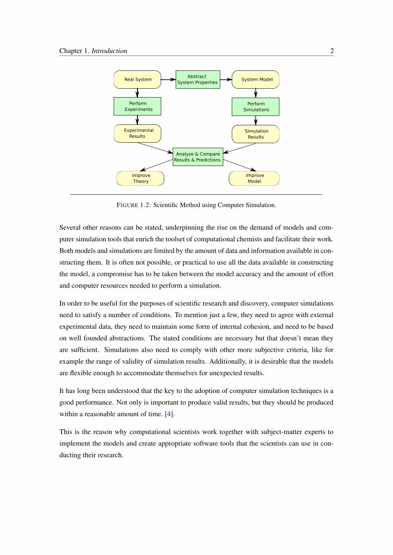
It cannot be disputed that computers today play a very significant role in the work of scientists
and researchers. A cursory glimpse of the scientific method traditional steps (see Figure 1.1),
compared to what nowadays happens in the lab reveals there has been a profound change in the
way scientists do their work, motivated mainly by the use of computer modelling and simulation
software (see Figure 1.2).
Observation
of Nature
Construct
Hypothesis
Perform
Experiments
Analyze
Data
Draw
Conclusions
FIGURE 1.1: Scientific Method Steps.
It is no longer common that all theories have to be subject to experimentation in order to dis-
prove them. It is increasingly the case that scientists will state their hypothesis in terms of
mathematical models, which can be easily translated into computer simulation codes [3]. If the
computer simulation arrives to negative or not statistically significant results, it is sometimes
more than enough to stop before undergoing costly, time consuming experiments.
Is also the case that for some experiments, scientists would like to perform; the available re-
sources are scarce or have been limited, either because of the cost or because of the danger
involved in its handling in the laboratory. In such cases, before undergoing experimentation,
scientists want to be reassured through the use of computer simulations that their hypotheses are
backed up by simulation data.
1
Chapter 1. Introduction 2
Real SystemAbstract
System PropertiesSystem Model
Perform
Experiments
Perform
Simulations
Experimental
ResultsSimulation
Results
Analyze & Compare
Results & Predictions
Improve
Theory
Improve
Model
FIGURE 1.2: Scientific Method using Computer Simulation.
Several other reasons can be stated, underpinning the rise on the demand of models and com-
puter simulation tools that enrich the toolset of computational chemists and facilitate their work.
Both models and simulations are limited by the amount of data and information available in con-
structing them. It is often not possible, or practical to use all the data available in constructing
the model, a compromise has to be taken between the model accuracy and the amount of effort
and computer resources needed to perform a simulation.
In order to be useful for the purposes of scientific research and discovery, computer simulations
need to satisfy a number of conditions. To mention just a few, they need to agree with external
experimental data, they need to maintain some form of internal cohesion, and need to be based
on well founded abstractions. The stated conditions are necessary but that doesn’t mean they
are sufficient. Simulations also need to comply with other more subjective criteria, like for
example the range of validity of simulation results. Additionally, it is desirable that the models
are flexible enough to accommodate themselves for unexpected results.
It has long been understood that the key to the adoption of computer simulation techniques is a
good performance. Not only is important to produce valid results, but they should be produced
within a reasonable amount of time. [4].
This is the reason why computational scientists work together with subject-matter experts to
implement the models and create appropriate software tools that the scientists can use in con-
ducting their research.
Chapter 1. Introduction 3
1.2 Motivation: Open Babel
In starting this research our primary motivation was to learn more about the technologies in use
for high performance computing using GPU. The second motivation was to work in an open
source project, so that any benefits achieved from doing the work could be contributed back to
the community afterwards.
The selected project was Open Babel, a cheminformatics software, which is commonly used
as a format inter-conversion tool, and it is also commonly referred to as a cheminformatics
swiss-knife [5]. OpenBabel is on the one hand a suite of programs tailored to serve the research
community in computational chemistry and biochemistry and on the other hand a C++ frame-
work with bindings for several other popular programming languages. The framework allows
a programmer to make use of OpenBabel popular tools from within other programs, essentially
giving the users the ability to extend and customize OpenBabel and make it suitable for their
own purposes.
The most well-known and publicized feature of OpenBabel is its conversion engine. In our
project however we were interested in tasks demanding a sheer amount of raw computing power,
therefore our focus was shifted to a less known capability of OpenBabel, namely its ability to
evaluate a molecule’s energy, by applying forcefields modeling.
Molecular forcefields modeling, as we will discuss further, is an interesting problem with many
interesting and useful applications that we will also mention. The reason to choose to focus on
forcefields from the high performance computing perspective responds to the fact that molecular
forcefields models are particularly amenable to parallelization.

Chapter 2
Background Theory
The theory of molecular mechanics forcefields modelling is very rich and requires a good com-
mand of physics and chemistry to be understood. In the present treatment, it is not our intention
to cover it exhaustively, but to give an overview, from which the implications in terms of mod-
eling, computing and validity of their use can be appreciated. Most of the material used in this
chapter has been adapted from Leach’s excellent book on molecular modelling [6]. Interested
readers are therefore encouraged to refer to that book as a primary source of information.
2.1 Molecular Mechanics
Molecular mechanics is a common term that is used to refer to a set of empirical equations
(models) that are used to describe the interactions between the atoms of a molecule and the
associated energies. Equations used are derived from classic laws of physics, in which atoms
are represented as particles, only considering their nuclei and ignoring their associated electrons.
In this kind of static models, atoms are connected by fixed bonds, meaning that it is not possible
to simulate reactions involving atoms changing their chemical composition (chemical structure).
2.2 Molecular Mechanics Force Fields
Forcefields in their highest level representation are given as finite sums of different kinds of
energy contributions that all together sum up to arrive to a total energy number.
4
Chapter 2. Background Theory 5
The individual sum terms have been parameterized and depend on fixed constants that have been
obtained experimentally and that are specific for each type of atom and interaction.
2.3 Molecular Force Fields vs Quantum Mechanic Methods
The reason why molecular force fields are so popular is that, compared with the more general
quantum mechanics methods, they don’t need to deal with the same level of detail and complex-
ity, while still being able to produce results with a good level of agreement with experimental
data. Molecular mechanics models have been repeatedly used to simulate problems which will
be otherwise too large from a quantum mechanics perspective.
Because Molecular Mechanics essentially ignore the electrons, they cannot be used to predict
properties depending on the electronic distribution of molecules.
2.4 Validity of Molecular Mechanics Methods
What stands at the core of molecular mechanics validity is the Born-Oppenheimer approxima-
tion, which says it is possible to calculate the energy of a molecule as a function of the nuclear
coordinates of the molecule elements (atoms).
Another key aspect of molecular mechanics models is their transferability. This property means
that a set of parameters developed and tested for a small subset of molecules can be generalized
to a complete family of compounds with a similar composition. And most importantly, data
obtained for small molecules may be used to study much larger molecules.
2.5 Molecular Force Fields General Form
Most of the forcefields in common use employ a simple four-component description of the intra-
and inter- molecular forces of a system (see Eq. 2.1). Empirically derived formulas are used to
describe how the overall energy of a system changes as bonds are pulled apart, rotated or bended.
Forcefields also consider terms to account for the interactions between non-bonded pairs (see
Figure 2.1).

Chapter 2. Background Theory 6
ϑ(~rN ) =∑bonds
ki2
(li − li,0)2 +∑
angles
ki2
(θi − θi,0)2 +∑
torsions
Vn2
(1 + cos(nω − γ))
+N∑i=1
N∑j=i+1
(4εij
[(σijrij
)12
−(σijrij
)6]
+qiqj
4πε0rij
) (2.1)
Next we will discuss the purpose and characteristics of each of these components:
The first term, known as the bond component, models the interaction between pairs of bonded
atoms, the most favored model is that of an harmonic potential where energy increases as the
bond length λi deviates from a base reference value λi,o.
Second term, the angle deformation component is modelled also as a harmonic potential using
the valence angles. A valence angle is the term used to name the angle formed between three
atoms A-B-C in which atoms A and C are both bonded to B.
The third term, the rotational component models how energy changes as a bond rotates along its
longitudinal axis.
The fourth contribution accounts for the non-bonded pairs interactions. These interactions occur
between atoms of different molecules (intermolecular), but they can also happen between atoms
of the same molecule (intra-molecular). For the last case, the condition is the bond separation
distance between atoms has to be of three bonds as a minimum. Non bonded interactions have
the form of a Coulomb potential in case of electrostatic forces and Lennard-Jones potential for
van der Waals interaction.
2.6 Empirical Nature of Force Fields
Forcefields models take the form of best fit for purpose mathematical equations. That is, there is
no correct form for a forcefield. The reason why forcefields in common use have a very similar
form is that, from an experimental point of view, the empirically derived formulas perform better
while doing predictions.
The functional form used for molecular mechanics forcefields is a trade-off between accuracy
and computational efficiency. Some very accurate functional forms can be very computation-
ally expensive, ruling them out for all practical purposes. However, as computer performance
increases, some of the more accurate functional forms have been incorporated into the models.

Chapter 2. Background Theory 7
FIGURE 2.1: Bonded and non-bonded particle interactions.
2.7 Atom Types in Molecular Mechanics Forcefields
All forcefields introduce the concept of atom type. The atom type is used to define the forcefield
parameters used in the calculation of the forces exerted on it. For a molecule (system) energy to
be determined, it is first necessary to assign an atom type to each atom in the system.
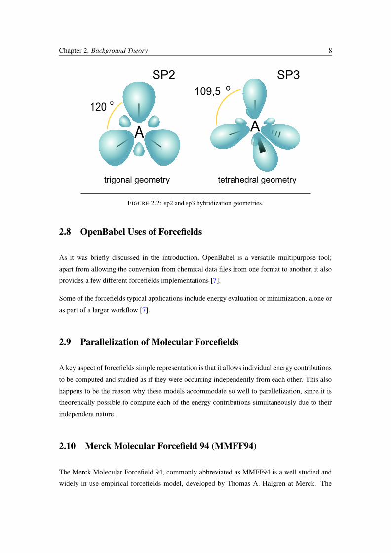
The atom type considers not only the atomic number of an atom; but it also contains informa-
tion about its hybridization state and in some cases the local environment. Moreover, forcefields
models distinguish between sp3-hybridized carbon atoms (tetrahedral geom.), sp2-hybridized
carbons (trigonal geom.) and sp-hybridized carbons (linear geom.). The parameters of a force-
field are expressed in terms of the atom type. For example the reference angle for a tetrahedral
carbon, θo, is 109.5 deg. The same property for an sp2-hybridized carbon is about 120 deg (see
Figure 2.2).
Chapter 2. Background Theory 8
A
120 o
A
109,5 o
SP3SP2
trigonal geometry tetrahedral geometry
FIGURE 2.2: sp2 and sp3 hybridization geometries.
2.8 OpenBabel Uses of Forcefields
As it was briefly discussed in the introduction, OpenBabel is a versatile multipurpose tool;
apart from allowing the conversion from chemical data files from one format to another, it also
provides a few different forcefields implementations [7].
Some of the forcefields typical applications include energy evaluation or minimization, alone or
as part of a larger workflow [7].
2.9 Parallelization of Molecular Forcefields
A key aspect of forcefields simple representation is that it allows individual energy contributions
to be computed and studied as if they were occurring independently from each other. This also
happens to be the reason why these models accommodate so well to parallelization, since it is
theoretically possible to compute each of the energy contributions simultaneously due to their
independent nature.
2.10 Merck Molecular Forcefield 94 (MMFF94)
The Merck Molecular Forcefield 94, commonly abbreviated as MMFF94 is a well studied and
widely in use empirical forcefields model, developed by Thomas A. Halgren at Merck. The
Chapter 2. Background Theory 9
forcefield is known for producing results very much in agreement with experimental data for
a large range of organic molecules. It has been found the model describes non-bonded inter-
actions between ligands and proteins very well, making it suitable for a whole range of useful
applications (i.e. molecule docking).
2.11 Uses of Forcefields Models
Molecular mechanics forcefields find their use in computational chemistry for energy evaluation
or energy minimization purposes, either alone or as part of a workflow [8]. Each forcefield has
been optimized for a particular family of compounds. In particular MMFF94 validity has been
tested and used against organic small sized molecules, the kind of molecules often used in in-
silico drug research [9].
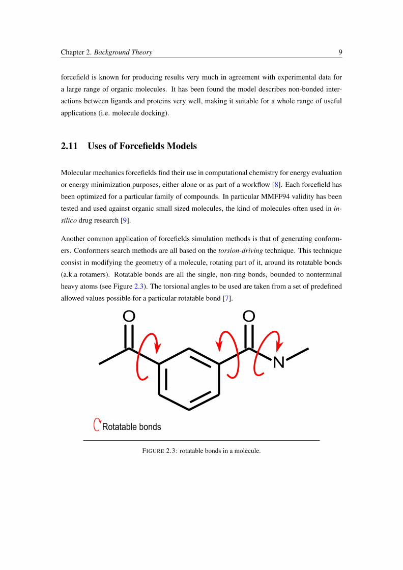
Another common application of forcefields simulation methods is that of generating conform-
ers. Conformers search methods are all based on the torsion-driving technique. This technique
consist in modifying the geometry of a molecule, rotating part of it, around its rotatable bonds
(a.k.a rotamers). Rotatable bonds are all the single, non-ring bonds, bounded to nonterminal
heavy atoms (see Figure 2.3). The torsional angles to be used are taken from a set of predefined
allowed values possible for a particular rotatable bond [7].
O
N
O
Rotatable bonds
FIGURE 2.3: rotatable bonds in a molecule.

Chapter 3
OpenBabel: A cheminformaticsframework
Chemical data is usually produced in a wide variety of different formats. Some of them have
become industry standards and other enjoy a less widespread adoption but are specific to some
specific tool or group. A common problem is to translate chemical data from one format into
another. In order to alleviate this problem, the open source community created OpenBabel, a
software tool for chemical data interconversion. In its current version, OpenBabel is capable to
read and write between more than a 100 formats [5].
For OpenBabel to perform this feat, it was necessary to develop a library of tools and algorithms,
that allow OpenBabel to hold a very complete internal representation of a molecule. This, in
turn, has made OpenBabel a platform, the use of which is no longer restricted to chemical data
interconversion but also capable of many other applications [7].
The key features of the OpenBabel framework are [7]:
• Extensive File Format Support
• Fingerprints and Fast Searching
• Bond Perception and Atom Typing
• Canonical Representation of Molecules
• Coordinate Generation in 2D and 3D
• Stereo-chemistry
10

Chapter 3. OpenBabel: A cheminformatics framework 11
• Forcefields
From this list of features in this research we will only be discussing the last one. But in order
to better understand some design decisions made during the project, we consider that it is also
important to understand the architecture and implementation of OpenBabel as a whole.
In this chapter the OpenBabel architecture and implementation is discussed. The build system
of the OpenBabel project is also introduced.
3.1 Open Babel Architecture
The Open Babel framework architecture (see Figure 3.1) has a modular design that reflects very
much the way in which the framework is intended to be used, both as a standalone set of tools
and as programmable library. For this same reason it supports several programming languages
bindings, all of them exposing a common API.
FIGURE 3.1: OpenBabel Framework Architecture.
OpenBabel base API, also commonly referred by OpenBabel developers as the Chemical Core,
contains OBMol, OBAtom, OBBond among with many other classes, that are used by Open-
Babel framework to create an internal description of a molecule. There is also a module in
charge of the conversion and management of chemical data formats that provides OpenBabel
with input/output capabilities.
Chapter 3. OpenBabel: A cheminformatics framework 12
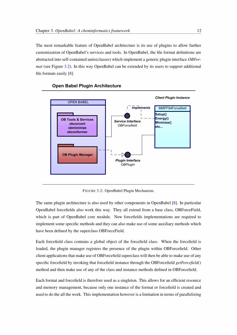
The most remarkable feature of OpenBabel architecture is its use of plugins to allow further
customization of OpenBabel’s services and tools. In OpenBabel, the file format definitions are
abstracted into self-contained units(classes) which implement a generic plugin interface OBFor-
mat (see Figure 3.2). In this way OpenBabel can be extended by its users to support additional
file formats easily [8].
Open Babel Plugin Architecture
OPEN BABEL
OB Tools & Servicesobconvert
obminimizeobconformer
OB Plugin Manager
MMFF94Forcefield
Setup()Energy()Minimize()etc...
Client Plugin Instance
Plugin InterfaceOBPlugin
Service InterfaceOBForcefield
implements
FIGURE 3.2: OpenBabel Plugin Mechanism.
The same plugin architecture is also used by other components in OpenBabel [8]. In particular
OpenBabel forcefields also work this way. They all extend from a base class, OBForceField,
which is part of OpenBabel core module. New forcefields implementations are required to
implement some specific methods and they can also make use of some auxiliary methods which
have been defined by the superclass OBForceField.
Each forcefield class contains a global object of the forcefield class. When the forcefield is
loaded, the plugin manager registers the presence of the plugin within OBForcefield. Other
client applications that make use of OBForcefield superclass will then be able to make use of any
specific forcefield by invoking that forcefield instance through the OBForcefield getForcefield()
method and then make use of any of the class and instance methods defined in OBForcefield.
Each format and forcefield is therefore used as a singleton. This allows for an efficient resource
and memory management, because only one instance of the format or forcefield is created and
used to do the all the work. This implementation however is a limitation in terms of parallelizing
Chapter 3. OpenBabel: A cheminformatics framework 13
molecule energy minimization tasks, which have to be pipelined one at a time, in order not to
overwrite the memory structures associated to each system/molecule during the forcefield setup.
3.2 Open Babel Implementation
Open Babel is implemented in C++. It is a cross-platform project supported in the latest ver-
sion of major operating systems (Windows, Mac OS X, Linux). For its compilation it uses
CMake [8]. CMake is an open-source, cross-platform build system. CMake handles the analy-
sis of dependencies needed to compile and build Open Babel for a particular target architecture.
CMake manages the generation of native makefiles and also integrates tightly with other popular
open-source programs like CTest (unit testing framework) and CDash (distributed testing and
reporting software) [10].
OpenBabel has some few external dependencies. External dependencies are checked by CMake
during the build preparation step. In case a dependency cannot be satisfied that will be reported
to the user during the configuration. However because dependencies are optional, OpenBabel
build will still be completed. The effect of building OpenBabel ignoring dependencies is that
some additional functionality and file format support will be sacrificed. For example in case the
XML development libraries cannot be found, OpenBabel will then not support the use of XML
formats [8].
There is some clear advantage in working with a minimal version of OpenBabel (i.e. compiling
without external dependencies) in the sense that the overall build process takes less time to
complete, which is specially useful for OpenBabel development purposes.
Apart from C++, OpenBabel provides bindings for other programming languages, most notably
for ”dynamic” scripting languages like Python. The purpose of these interfaces is to enable
rapid prototyping and development [8].
In the case of developing extensions (plugins) to the library, OpenBabel require those to be
written in C++. Plugins are dynamically loaded at runtime. The purpose is to reduce OpenBabel
memory footprint, but as it has been discussed in the previous section, this approach has the
disadvantage of supporting only a single instance of the plugin living in memory at a time,
therefore concurrent processing of several molecules at a time is not supported.
Chapter 3. OpenBabel: A cheminformatics framework 14
3.3 OpenBabel Development
OpenBabel is developed and distributed using an open-source model. This model encourages
third-party users of the library to get involved and to contribute to OpenBabel development. At
the very least, OpenBabel license grants the user the rights to study how the software works, to
modify it and to share those modifications with others [8].
Open source development model is comparable with the way scientific research is conducted in
an open peer-reviewed environment, allowing results cross-validation, repetition and building
on previous research. The developers of Open Babel, being scientists themselves, believe in this
model and actively encourage it, by documenting, discussing and conducting all development
using public forums, wikis and public code repositories [8].
As a matter of fact, that was one of the main personal motivations, encouraging us to work on
this project, in order to contribute and enrich OpenBabel, and get a general impression on how
open development works from the inside.
3.4 Open Babel Forcefields Uses
Eventually, we want to describe how forcefields, and in particular MMFF94, are used by the
library. Open Babel uses forcefields in four different ways (command line tools):
Energy Evaluation (obenergy)Given a molecule 3D structure, this application calculates the energy of the molecule/sys-
tem configuration applying one of OpenBabel’s molecular force fields models.
Energy Minimization (obminimize)Given an unoptimized 3D molecular structure, it will apply the MMFF94 energy compu-
tation routines iteratively using the Conjugate Gradient method to obtain a low energy,
optimized 3D molecular structure.
Conformers Generation (obconformer)This tool can be used as part of a conformational study pipeline. It works by generating
and comparing a random set of conformers. The desired number of conformers to gen-
erate, and the minimization steps used to optimize them are given as parameters to the
application. The best conformer of the set – the one having the lowest energy – is the
application output.
Chapter 3. OpenBabel: A cheminformatics framework 15
Conformers Generation (confab)Confab is a separate tool, devoted to conformers generation, that internally works by call-
ing OpenBabel forcefield methods. The reason confab is not part of OpenBabel is due to
license restrictions regarding one of its dependencies. The goal of this tool is different
from the one included in OpenBabel distribution. Confab is set to efficiently and compre-
hensively explore the space of conformers for a given molecule. It will generate several
conformers at a time. They will not necessarily represent the lowest energy molecule
arrangements, but will be within a cutoff energy threshold passed as an argument to the
program [11].
Chapter 4
Validation and Testing Methodology
4.1 Selection of the Validation Dataset
In this research, we make use of three different molecule datasets. The datasets served different
purposes. We used one particular dataset to validate the MMFF94 after each major modification.
Every time a performance optimization work is carried out, special care should be given to
validate that any of the changes introduced don’t break the program.
Also, because of the complexity of the codes, it is very possible that an error introduced while
doing the optimization work goes undetected, if the input data is not sufficiently rich. Because
we are not that familiar with MMFF94, it would have been very difficult to come up with a
dataset sufficiently diverse to validate the optimized MMFF94 implementation by ourselves.
Fortunately, Merck, the same company where MMFF94 was originally developed, has been
kind enough to also provide an accompanying validation suite, so that particular MMFF94 im-
plementations can be tested against [12].
The MMFF94 validation suite, in its current form, consists of 761 structures, molecules and
ions. The structures were derived for a crystallographic structure database maintained by the
Cambridge Crystallographic Data Center. The suite has been constructed to test all MMFF94
model parameters and empirical-rule procedures [12]. The MMFF94 parameter files are also
available in Internet at the following ftp address: MMFF94 Parameters FTP Site
Apart from the input files and data, the validation suite also contains exemplary output files
obtained using OPTIMOL and BatchMin [12]. More information about how the validation suite
16
Chapter 4. Validation and Testing Methodology 17
should be used and further details on its compilation can be found on this website: MMFF94
Validation Suite Website.
4.2 Selection of the Testing Dataset
In our case, we were not only interested in validating the implementation, but also in testing its
performance. We could have used the validation suite provided by Merck also for this purpose,
but after careful consideration, we determined it was a better idea to use a different one, for
three reasons:
1. The Merck validation dataset is huge. This makes it impractical for both processing and
reporting, especially when plotting the performance of an optimized MMFF94 model
implementation for each of the structure comprising the dataset.
2. The second reason is that structures and molecules in the validation suite have their ge-
ometry already optimized in order to both speedup the energy calculation and avoid that
any final conformation in the validation dataset represent a shallow local minimum on
MMFF94 surface, in which case an optimizer would converge to a different local min-
imum, inadvertedly implying an issue with an otherwise totally correct MMFF94 im-
plementation [12]. However an optimized geometry would also mean that the num-
ber of minimization steps would always be very small, effectively limiting our capac-
ity of testing the performance of OpenBabel’s applications such as obminimize and
obconformer.
3. Finally, because one of our purposes was to test the performance of OpenBabel’s con-
former generators (obconformer and confab), we thought it was also important to
have a dataset consisting of molecules with a varied number of conformers (rotatable
bonds).
Our first idea was to build the performance testing dataset ourselves, but this task proved to be
difficult for many reasons, in particular a lack of knowledge of the public chemical library, and
incomplete understanding of the validity range for MMFF94 model.
Fortunately, in cheminformatics literature there is already abundant discussion on the subject so
it wasn’t hard to find and pick some publicly available datasets. We ended up choosing two, a
dataset from Borodina et al. [13] and a dataset from Bostrom et al. [14]. The Borodina dataset
consists of 1000 small molecule crystal structures. This dataset represents bioactive conformers,

Chapter 4. Validation and Testing Methodology 18
not all of them are of interest because some cannot be handled by MMFF94 forcefield, and
others have no rotatable bonds [11]. From the remaining molecules we randomly chose 300 to
do our initial performance testing. We also wanted to have a smaller, representative dataset, for
statistics and performance plotting purposes. We decided upon the Bostrom dataset because it is
compact – it contains 36 molecules ranging from 1 to 11 rotatable bonds [14]– yet representative
of the kind of small-sized molecules in common use in drug research[15].
4.3 Molecules Classification
Molecules can be classified using several different criteria. In Cheminformatics, it is common
to classify molecules regarding their size. It turns out that the size of the molecule is directly
related with its biological purpose and scientific applications. Molecules are separated in two
main groups: small and big molecules. The boundaries between these two groups are not clear-
cut, an approximate guide is provided measuring a molecule size in terms of its Molecular
Weight (MW).
1. Small Molecular Weight (SMWs): These are small sized molecules, whose upper molec-
ular weight limit is around 700 Daltons[16]. Small molecules are of interests to scientists
because they are used as ligands. Their small size allows them to penetrate the membrane
of cells. In the fields of pharmacology and biochemistry, hundreds of thousands of these
molecules are studied, looking for highly selective molecules that attach only to a partic-
ular kind of protein. Other common uses of small molecules are as cell signal triggers,
and as pesticides in farming[16]. Most of the drugs fall into these category, although not
all drugs are small sized molecules.
2. High Molecular Weight (HMWs): In this category fall the polymers, peptides and pro-
teins. These molecules are of high interest in pharmaceutical applications. For example
peptides are used for diagnostics and vaccines. Proteins are essential to the structure and
function of cell and viruses and therefore actively studied in biochemistry[17].
The size of a molecule is an important criteria to have in mind, when doing computer simula-
tion. Depending on the algorithm, in general big molecules will demand more computational
resources from the system. In particular, in the case of OpenBabel, we are restricted to study
SMWs, the reason being that OpenBabel MMFF94 implementation will read the molecule and
pre-calculate results for each pair of non bonded atoms. For example van-der-Waals energy cal-
culation term,OBFFVDWCalculationMMFF94, uses 228 bytes and the electrostatic energy
Chapter 4. Validation and Testing Methodology 19
contribution term, OBFFElectrostaticCalculationMMFF94, uses 140 bytes. Consid-
ering a big molecule, say one having 4, 000 atoms, the memory requirements, will easily exceed
the physical memory available in current systems.
Open Babel’s
Non-Bonded Interactions 4, 0002 ∗ (228 bytes+ 140 bytes) = 5.6 GB
Memory Requirements
As an aside comment, it could be possible to optimize the current MMFF94 implementation
in OpenBabel, for example by making use of a NeighbourList to only compute non-bonded
interactions within a given threshold [18].
For the case of MMFF94 method, both the van-der-Waals and electrostatic interactions drop to
zero as the inter-atomic distance increases, effectively reducing the algorithm complexity and
memory requirements from O(n2) to O(n log n). However, in our opinion, this would have
required a major rewrite of the code, and defeat the purpose of exploring acceleration using
parallel programming techniques.
Chapter 5
Performance Profiling
5.1 Profiling OpenBabel
We were interested in determining how the different applications that make use of MMFF94
model behave with regard to the use of processor resources. As we previously stated in previous
chapters, we expected that an important fraction of the computation would be spent in the non-
bonded interaction terms. Still in order to have an idea of the application speedup, according
to Amdahl’s law, and in order to confirm our predictions we profile the applications using two
different approaches:
• automatic instrumentation
• coarse-grained time measurements
5.1.1 Profiling MMFF94 using a profiling framework (OProfile)
For our first round of measurements, we experimented with two different profiling frameworks:
gprof and OProfile. Both of them are similar in nature, they are designed to collect and
record data during program execution. The way they work is by instrumenting the source code
of the application that we want to profile, inserting calls to the instrumentation library into the
application’s code [19].
Then later when the application is executed, the calls are registered and processed by the frame-
work. This approach gives us a rough idea of how time is used by the application library, the
20
Chapter 5. Performance Profiling 21
methods consuming more application cycles will rank higher. Profiling frameworks proved us
with an estimate of the cumulative spent in a method and its child routines. The accuracy of this
profiling technique depends on an appropriate selection of the CPU counters to be observed and
the input data being representative of a common application workload [19].
When doing the profiling we realize that gprof doesn’t support profiling codes that make use
of shared (dynamic) libraries. OpenBabel applications link dynamically at runtime with the
OpenBabel library. So at the beginning when doing profiling we couldn’t get any output. This
motivated us to try with a different profiling framework: OProfile.
Oprofile doesn’t create the nice output call graphs we can get from gprof, but it is more
configurable, and what is crucial is that it also supports profiling applications that make use
of dynamic linked libraries (shared libraries). Oprofile allow us to watch different register
counters (events). For our study we chose the default one (CPU CLK UNHALTED).
A sample of the kind of output we got from this tool can be appreciated on Figure 5.1.
A closer inspection of the results from the application’s profile shows us two things. First,
as we were already expecting, the application is spending most of its time computing the non-
bonded interactions. The second revelation, however, is more surprising. There are several static
methods from the forcefield superclass that have not been inlined in the MMFF94 forcefield
implementation, this could translate into a performance drop. The third thing we observed is
that the percentage of time spent on the computation of the forcefield is not as large as we were
expecting, therefore the performance gain we could achieve using parallelization will be modest,
unless we can identify additional sources of parallelism.
5.1.2 Profiling MMFF94 using custom timers
Even if the amount of information we gain by the use of a profiling framework could already
give us a rough idea of which are the computationally intensive kernels in our application, we
realize that we needed to have more information on the particular behaviour of each of the
applications using the MMFF94 forcefield.
For this reason, we decided to time the performance of specific sections of the code using custom
timers. The advantage of this approach is also that later on we can use this same metrics to
compare different MMFF94 implementations. We were primarily interested in three different
measurements for each application:
TIME READ Time spent reading a molecule.

Chapter 5. Performance Profiling 22
CPU: Intel Architectural Perfmon, speed 1600 MHz (estimated)Counted CPU_CLK_UNHALTED events (Clock cycles when not halted)with a unit mask of 0x00 (No unit mask) count 12000samples % image name symbol name----------------------------------------------------------------13316 6.9366 libopenbabel.so.4.0.0OpenBabel::OBForceField::VectorDivide(double*, double, double*)12735 6.6339 plugin_forcefields.so voidOpenBabel::OBFFVDWCalculationMMFF94::Compute<false>()11612 6.0489 libopenbabel.so.4.0.0OpenBabel::OBForceField::VectorSubtract(double*,double*,double*)10354 5.3936 libopenbabel.so.4.0.0OpenBabel::OBForceField::VectorLength(double*)7815 4.0710 libm-2.11.1.so cos7012 3.6527 libm-2.11.1.so __ieee754_sqrt5105 2.6593 libm-2.11.1.so __ieee754_acos4262 2.2202 libm-2.11.1.so __ieee754_atan23571 1.8602 libopenbabel.so.4.0.0OpenBabel::OBForceField::VectorDot(double*, double*)3317 1.7279 libm-2.11.1.so sqrt3314 1.7263 plugin_forcefields.soOpenBabel::OBForceField::VectorDistance(double*, double*)3087 1.6081 libopenbabel.so.4.0.0OpenBabel::OBForceField::VectorCross(double*, double*, double*)3030 1.5784 libopenbabel.so.4.0.0vector<OpenBabel::OBBond*>::iterator::__normal_iterator(OpenBabel::OBBond** const&)2749 1.4320 plugin_forcefields.so voidOpenBabel::OBFFVDWCalculationMMFF94::Compute<true>()
-- truncated output ---
FIGURE 5.1: Performance Profiling obminimize (OProfile)
TIME SETUP Time to setup the forcefield and precalculate forces.
TIME COMPUTE Time spent in computation.
5.2 Profiling Methodology and Results
The profiling methodology consisted in modifying each application using the MMFF94 force-
field model. As it was mentioned before, we were interested in recording the timings for each
major execution bracket (input, setup and computation).
Chapter 5. Performance Profiling 23
We also recorded some other values from each molecule in the dataset, in order to do the anal-
ysis. In particular for each molecule from the dataset, we recorded its mass, number of heavy
atoms (non-H atoms), number of conformers and number of rotamers.
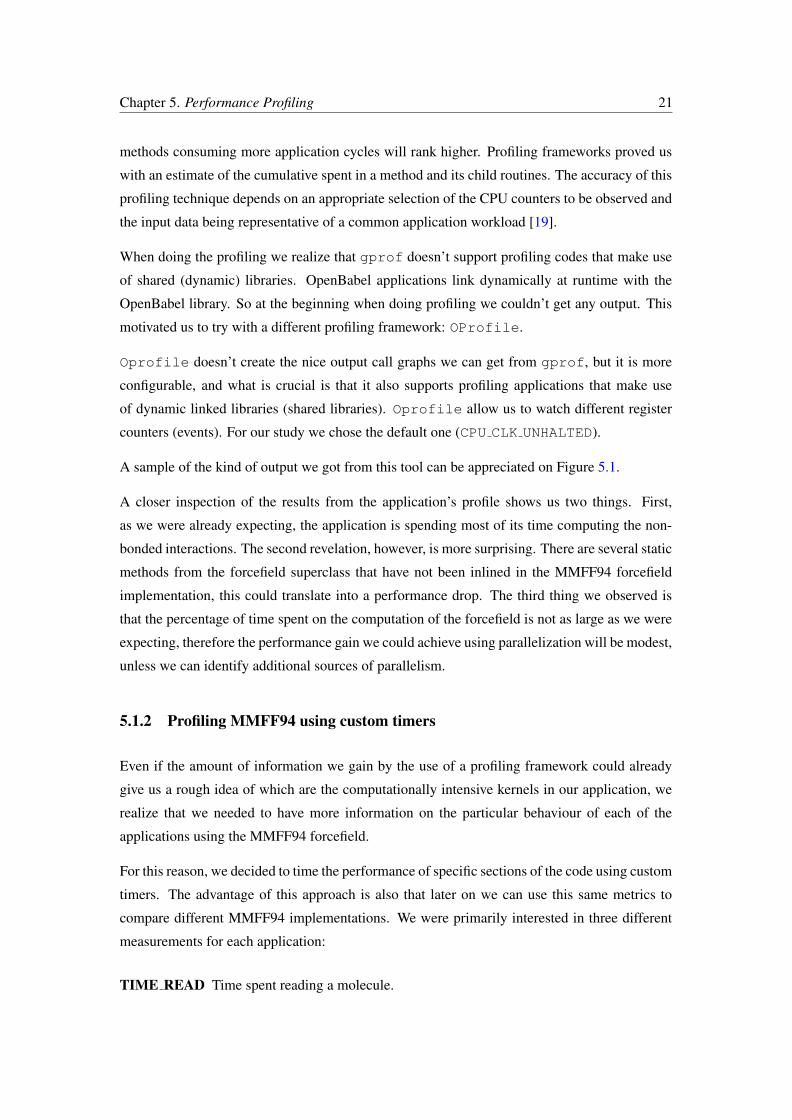
We then produced several different plots, to help us better understand each application. In par-
ticular we found useful to plot the execution time breakdown for each molecule in the Bostrom
dataset, against the size of the molecule, given by the number of heavy atoms in molecule. The
intuition was that overall execution time will increase progressively as the size of the molecule
gets larger.
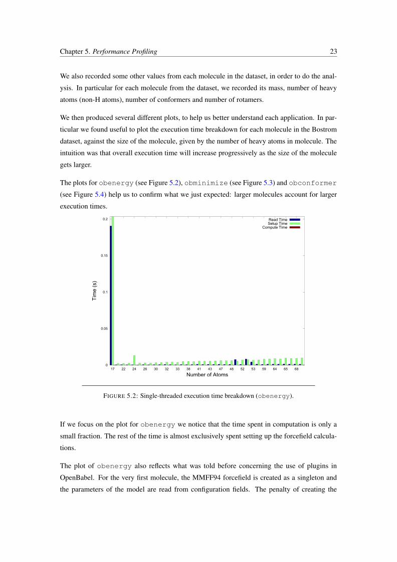
The plots for obenergy (see Figure 5.2), obminimize (see Figure 5.3) and obconformer
(see Figure 5.4) help us to confirm what we just expected: larger molecules account for larger
execution times.
0
0.05
0.1
0.15
0.2
17 22 24 26 30 32 33 38 41 43 47 48 52 53 59 64 65 68
Tim
e (s
)
Number of Atoms
Read TimeSetup Time
Compute Time
FIGURE 5.2: Single-threaded execution time breakdown (obenergy).
If we focus on the plot for obenergy we notice that the time spent in computation is only a
small fraction. The rest of the time is almost exclusively spent setting up the forcefield calcula-
tions.
The plot of obenergy also reflects what was told before concerning the use of plugins in
OpenBabel. For the very first molecule, the MMFF94 forcefield is created as a singleton and
the parameters of the model are read from configuration fields. The penalty of creating the
Chapter 5. Performance Profiling 24
0
0.1
0.2
0.3
0.4
0.5
0.6
0.7
7 9 13 24 31 37 39 60 66 640
Tim
e (s
)
Number of Atoms
Read TimeSetup Time
Compute Time
FIGURE 5.3: Single-threaded execution time breakdown (obminimize).
0
50
100
150
200
17 22 24 26 30 32 33 38 41 43 47 48 52 53 59 64 65 68
Tim
e (s
)
Number of Atoms
Read TimeSetup Time
Compute Time
FIGURE 5.4: Single-threaded execution time breakdown (obconformer).

Chapter 5. Performance Profiling 25
forcefield is clearly visible, despite the first molecule from the Bostrom dataset being also the
smallest one.
In the case of the plot for the obminimize application, what we could observe is that the
time spent for setting up the forcefield and performing calculations are comparable. In this
plot also the time spent reading the molecule and loading the parameters for the MMFF94
implementation is almost negligible.
Finally, for the case of the obconformer application, we saw that the execution time is com-
pletely dominated by the computation of the forcefield. What this plot also shows is that for
relatively small molecules, the execution time for the application is already perceptible by the
user.
5.3 Performance Results Conformers Generation (confab)
In the case of conformers generation using confab, we wanted to find out particular informa-
tion concerning the application execution behaviour as the number of conformers and rotatable
bonds increases (see Figure 5.5. Here, our intuition tells us that the time fraction spent in compu-
tation was going to increase linearly with the number of rotatable bonds. Looking at the profile,
this criteria doesn’t hold all the time, but it can still be used as a good performance predictor.
For example we can think in an implementation where this criteria is taken into account in order
to decide whether the current MMFF94 implementation or a GPU accelerated version should be
used. Notice, this plot also shows some scaling preliminary results, but their discussion is left
for the next chapter.
In the case of confab we also do the profiling using the Borodina dataset. This dataset is larger
and therefore comprises a more complete sample of the kind of structures that scientists are
normally interested in generating conformers for. Looking at the plot for the Borodina dataset
(see Figure 5.6) , we could also tell that molecules with a large number of rotatable bonds are
not equally represented in the suite.
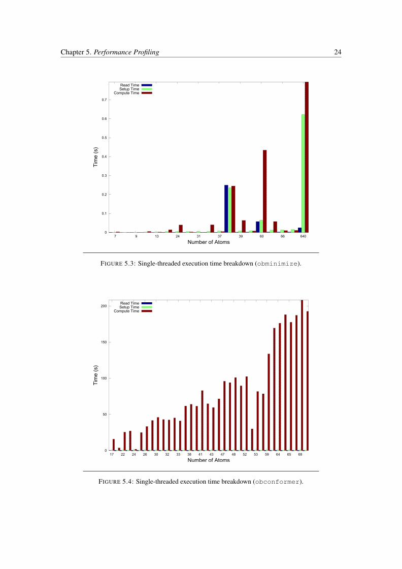
While confab will perform well for molecules with a small number of rotatable bonds, its
performance will drop dramatically for molecules with eight or more rotatable bonds. This was
observed even for some of the relatively small molecules in the dataset (see Figure 5.7). We can
conclude that the number of rotatable bonds on a molecule is an stronger predictor of confab
performance than the molecule size (number of atoms).

Chapter 5. Performance Profiling 26
0. 8
0. 82
0. 84
0. 86
0. 88
0. 9
0. 92
0. 94
0. 96
0. 98
1
0 2 4 6 8 10 12
Com
pute
Tim
e F
ract
ion
(con
fab)
Number of Rotamers
Si ngl e Thr eadTwo Thr ead
Four Thr ead0
5
10
15
20
25
30
0 200 400 600 800 1000 1200
Num
ber
of M
olec
ules
Total CPU Time (s)
Bost r om Set ( Si ngl e Thr ead)
FIGURE 5.5: confab performance (Bostrom dataset).
0. 75
0. 8
0. 85
0. 9
0. 95
1
0 2 4 6 8 10 12
Com
pute
Tim
e F
ract
ion
(con
fab)
Number of Rotamers
Bor odi na Dat aset0
50
100
150
200
250
300
350
400
0 100 200 300 400 500 600 700 800
Num
ber
of M
olec
ules
Total CPU Time (s)
Bor odi na Dat aset
FIGURE 5.6: confab performance (Borodina dataset).
Chapter 5. Performance Profiling 27
400
200
Gen
erat
ion
Tim
e (s
econ
ds)
0
Number of Conformers
1000
800
600
150001000050000
Borodina Dataset1200
20000
8
2
6
10
Num
ber
of R
otam
er B
onds
4
FIGURE 5.7: confab performance (conformers vs rotatable bonds).
5.4 MMFF94 Memory Profile
One possible way of gaining information about OpenBabel’s MMFF94 forcefield implementa-
tion is to profile how the memory is being utilized by each particular computed term (see Figure
5.8). This particular plot is obtained by adding the size of the calculation objects created during
the forcefield setup.
Creating this kind of plot for the Bostrom dataset clearly shows the non-bonded interaction
terms, and in particular van-der-Waals calculations, are the ones using the largest amount of
memory. In MMFF94 the memory requirements will increase quadratically with respect to the
number of atoms in molecule.
A similar plot can be created but this time plotting the memory allocation pattern as the number
of atoms in the molecule increases (see Figure 5.9). This plot is not as interesting as the first
one we presented, however it shows straightforwardly that one of the important limitations for
OpenBabel’s MMFF94 implementation is the simulation size.

Chapter 5. Performance Profiling 28
30 40 50 60 70 8010 200
100000
200000
300000
400000
500000
600000
Number of Atoms
Allo
cate
d M
emor
y (b
ytes
)
Mem Bond Calc.Mem Angle Calc.
Mem StrBnd Calc.Mem Torsion Calc.
Mem OOP Calc.Mem VDW Calc
Mem Elect. Calc.
FIGURE 5.8: MMFF94 memory allocation breakdown.
300000
200000
100000
0
Mem
ory
Allo
catio
n (b
ytes
)
Number of Atom Pairs (Calculations)
500000
400000
3000200010000
Bostrom Dataset
50
30
20
60
40
70
Num
ber
of A
tom
s
FIGURE 5.9: MMFF94 memory requirements vs simulation size.

Chapter 5. Performance Profiling 29
5.5 MMFF94 Setup Profile
Although we are primarily interested in understanding the computation step of MMFF94, we
thought a plot showcasing the amount of calculation objects created for each molecule during
the forcefield setup could convey some extra information, useful to decide on how parallelization
will be carried out (see Figure 5.10).
0
500
1000
1500
2000
2500
3000
3500
17 18 23 24 26 27 31 32 33 37 39 41 43 43 47 48 52 53 55 59 64 64 68 68
Inde
pend
ent C
alcu
latio
ns
Number of Atoms
Bond Cal c.Angl e Cal c.
St r Bnd Cal c.Tor si on Cal c.
OOP Cal c.VDW Cal c
El ect . Cal c.
FIGURE 5.10: obenergy calculation objects size (MMFF94 Setup).
In this case, we were expecting that the number of calculation objects created for bot electro-
static and van-der-Waals interactions will be exactly the same, that is num atoms2. However,
in OpenBabel’s MMFF94 implementation this is not the case. Some additional considerations
are made at the time of setting up the forcefield that reduce the number of calculations for the
electrostatic contribution.
By looking at the code that is used to setup the electrostatic calculations, we found that the
atoms are not considered in isolation but as part of groups. Only atoms belonging to different
groups are considered in setting up the energy contribution. The way in which grouping is done
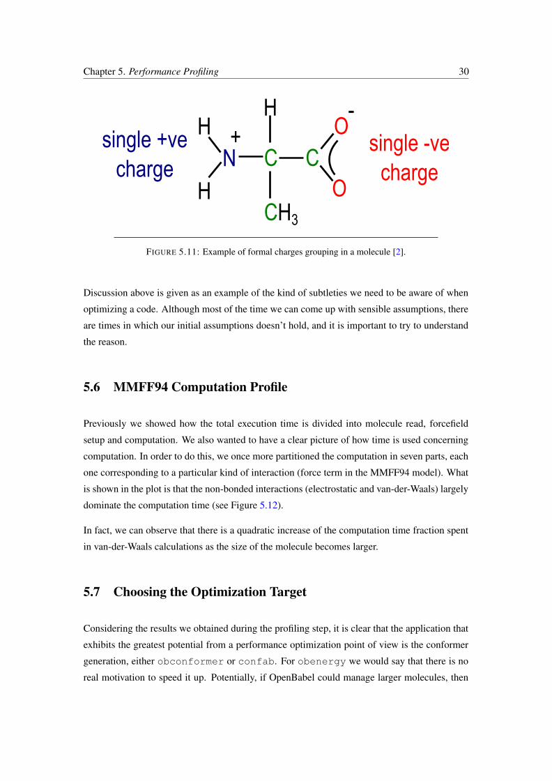
is by considering the formal charges of the molecule (see Figure 5.11). A group formal charge
shows whether an atom or group of atom gained or lost an electron [2]. This kind of grouping
is the reason why calculation objects for electrostatic contributions are less.
Chapter 5. Performance Profiling 30
H
H
N C C
CH3
O
O
single -vecharge
single +vecharge
H+
-
FIGURE 5.11: Example of formal charges grouping in a molecule [2].
Discussion above is given as an example of the kind of subtleties we need to be aware of when
optimizing a code. Although most of the time we can come up with sensible assumptions, there
are times in which our initial assumptions doesn’t hold, and it is important to try to understand
the reason.
5.6 MMFF94 Computation Profile
Previously we showed how the total execution time is divided into molecule read, forcefield
setup and computation. We also wanted to have a clear picture of how time is used concerning
computation. In order to do this, we once more partitioned the computation in seven parts, each
one corresponding to a particular kind of interaction (force term in the MMFF94 model). What
is shown in the plot is that the non-bonded interactions (electrostatic and van-der-Waals) largely
dominate the computation time (see Figure 5.12).
In fact, we can observe that there is a quadratic increase of the computation time fraction spent
in van-der-Waals calculations as the size of the molecule becomes larger.
5.7 Choosing the Optimization Target
Considering the results we obtained during the profiling step, it is clear that the application that
exhibits the greatest potential from a performance optimization point of view is the conformer
generation, either obconformer or confab. For obenergy we would say that there is no
real motivation to speed it up. Potentially, if OpenBabel could manage larger molecules, then

Chapter 5. Performance Profiling 31
0
0. 0001
0. 0002
0. 0003
0. 0004
0. 0005
17 18 23 24 26 27 31 32 33 37 39 41 43 43 47 48 52 53 55 59 64 64 68 68
Com
pute
Tim
e (s
)
Number of Atoms
E. Bond Cal c.E. Angl e Cal c.
E. St r Bnd Cal c.E. Tor si on Cal c.
E. OOP Cal c.E. VDW Cal c
E. El ect . Cal c.
FIGURE 5.12: obenergy computation breakdown (MMFF94 forcefield).
we could be interested in a faster version of obenergy as we can realize that the number of
calculations will dramatically increase.
To judge what will be the case for obminimize is perhaps more difficult. In the case of
obminimize, the execution not only depends on the size of the molecule being treated, but
also on how close the input molecule geometry is to the molecule’s optimal geometry(lowest
energy). This cannot be easily judged in advance, but it needs to be assessed as the optimization
progresses.
There is something obvious, but still, we would like to mention it. These three applications
don’t work in isolation, but rather depend on each other. In particular obconformer calls for
each conformer that it generates to obminimize which in turn calls obenergy. Therefore
an optimization to obenergy will translate to a speedup also in the other two.
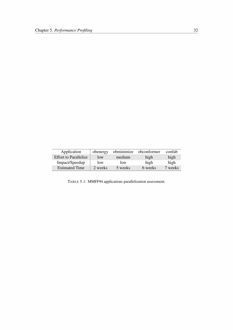
To close this chapter, we present a table judging the effort of parallelizing all of the applications
profiled and the perceived impact (speedup).
Chapter 5. Performance Profiling 32
Application obenergy obminimize obconformer confabEffort to Parallelize low medium high high
Impact/Speedup low low high highEstimated Time 2 weeks 5 weeks 6 weeks 7 weeks
TABLE 5.1: MMFF94 applications parallelization assessment.
Chapter 6
Optimizing MMFF94 (Single Core)
6.1 Vector Operations in OpenBabel
The computation of MMFF94 and other forcefields in OpenBabel, make use of common vector
operations like distance, cross and dot products. These operations, together with other common
code is currently provided by the base forcefield class OBForceField.
Given that most processors nowadays include some form of support for vectorization, we de-
cided an important step towards optimizing MMFF94, would be to optimize how vector opera-
tions are handled.
6.2 Eigen a Linear Algebra Template Library
There are several programming libraries with good support for vector operations (e.g. BLAS).
However, OpenBabel developer community has adopted Eigen, an optimized linear algebra li-
brary which is vector aware and has been optimized for performance in a wide range of architec-
tures, explicitly making use of the vectorization support facilities provided by the hardware [20].
6.3 MMFF94 Single Core Optimization Strategy
Eigen as every other programming library has its own idiosyncrasies, and it takes some time to
learn and start profiting from it. The advantage however is that due to the high level abstractions
introduced, the code end up being more compact and readable.
33
Chapter 6. Optimizing MMFF94 (Single Core) 34
Because of time limitations, we decided the better way to get up to speed with Eigen, was to
transform the MMFF94 code in a series of iterations, transforming first the computing terms
one at a time, and testing the validity of the energy computed terms after each transformation.
For this first step the memory structures created by the original MMFF94 were used and an
intermediate step was added in which the data was placed inside Eigen vectors before the actual
computation.
After all MMFF94 energy computation terms have been transformed to Eigen, a second set
of iterations started. In this step we transformed the setup of the MMFF94 forcefield, getting
rid of the former memory structures used by the previous MMFF94 implementation, making
use instead of Eigen vectors to store precomputed values. Every round of transformation was
followed by a results validation round.
This strategy helped us not only to avoid introducing hard to trace errors while porting the
code, but also gave us a better understanding of the forcefield implementation and OpenBabel
in general.
Apart from the computation and setup, MMFF94 implementation class, has many other methods
used for loading MMFF94 parameters and during forcefield setup. To avoid implementing those
methods, our Eigen enabled implementation subclasses MMFF94 implementation and overrides
the (setup) and (energy) methods from it (see Figure 6.1)
6.4 Benchmarking OpenBabel MMFF94 vs MMFF94+Eigen
While porting code is always a good idea to maintain at least two separate versions: stable and
development. This in order to easily debug any programming errors introduced while porting.
OpenBabel’s plugin model proved to be exceptionally helpful in this regard, because in order to
switch between the stable and development implementations we only had to change the force-
field parameter when running the obenergy application and the appropriate implementation
will then be loaded by the plugin mechanism.
Additionally this approach proved very useful to do the benchmarking of the Eigen enabled
implementation against the one currently use by OpenBabel. For the benchmarking we used
again the Bostrom dataset, only this time we didn’t show individual molecule benchmarks, but
an average of the individual performance of the implementation computing each of the energy
terms in the model. We do the same with the Eigen enabled version of the forcefield (see Figure
6.2).

Chapter 6. Optimizing MMFF94 (Single Core) 35
OBPlugin
+ TypeID()+MakeInstance()+ Init()+ GetID()
OBForceFieldMMFF94Eigen
+ Setup(OBMol &mol)+ Energy()
Class Diagram - MMFF94 + Eigen3
implementsOBForceField
+ SetupCalculations()+ Energy()
OBForceFieldMMFF94
+ SetupCalculations()+ Setup(OBMol &mol)+ Energy()- ParseParamFile()- SetTypes()- SetFormalCharges()- SetPartialCharges()
FIGURE 6.1: Eigen enabled MMFF94 implementation class diagram.
0
5e-06
1e-05
1.5e-05
2e-05
2.5e-05
3e-05
3.5e-05
4e-05
OpenBabel OpenBabel + Eigen3
Tim
e (s
)
σ1 = 4.7e-06, σ2 = 4.1e-06E. Angle Calc. σ1 = 5.5e-06, σ2 = 6.2e-06
E. StrBnd Calc. σ1 = 3.4e-06, σ2 = 3.9e-06E. Torsion Calc. σ1 = 1.4e-05, σ2 = 1.5e-05
E. OOP Calc. σ1 = 3.5e-06, σ2 = 3.9e-06E. VDW Calc. σ1 = 1.2e-05, σ2 = 1.6e-05
E. Elect. Calc. σ1 = 3.8e-06, σ2 = 4e-06
E. Bond Calc.
FIGURE 6.2: MMFF94 mean computation time benchmark (obenergy).

Chapter 6. Optimizing MMFF94 (Single Core) 36
6.5 Discussing MMFF94 Single Core Optimization Results
From the benchmarking plot is clear the Eigen enabled version is not giving a better performance
even after removing all Eigen preconditioning and enabling optimizations at compile time. We
were not expecting to find this, but we can still reason, that it probably has to do with memory
alignment problems and overheads introduced by the library.
Still we consider the use of Eigen is an enhancement in terms of improving code readability,
and certainly spending more time with the library could give us a better understanding and will
translate in a more efficient port. Some of the Eigen optimizations that we would like to explore
further would be array backed vectors and using matrices instead of vectors.
Also we estimate the performance of MMFF94 Eigen implementation will get better for bigger
molecules (large number of calculations).
Chapter 7
Optimizing MMFF94 (Multi-Core)
7.1 MMFF94 routines using OpenMP
During our first code revisions of MMFF94 in OpenBabel, we found some OpenMP directives
have already being added to the code. However by looking in the current documentation we
couldn’t found any mention about it.
After looking carefully in the archive of OpenBabel’s developer list and wiki, we found that
around 2008, one of OpenBabel developers add OpenMP directives to OpenBabel and do some
performance experiments with obminimize [21].
We proceed to compile the code using the latest development version of OpenBabel, and we real-
ize that despite the directives were there, the code was dormant. There was no explicit way to en-
able them during the project compilation, other than manually editing the CMakeCache.txt
file and adding the appropriate compiler flags there.
We did some additional research to understand why this was so, and we found that in the be-
ginning OpeBabel used Autotools to package and built the software, but later the framework
developers decided to change the built process to CMake. Presumably at this point is where
OpenMP support was lost.
7.2 Re-enabling OpenMP support in OpenBabel
The manual approach of editing the CMakeCache.txt file although being sufficient for de-
velopment purposes is not practical for packaging the modifications and made them available to
37

Chapter 7. Optimizing MMFF94 (Multi-Core) 38
other users, in particular the ones less familiar with programming.
For this reason, we decided to find out the way to re-enable OpenMP during the build process.
CMake is extremely powerful and enabling OpenMP was quite easy. It took less than 10 lines,
that were introduced into the build configuration file (CMakeLists.txt):
1 # / / T e s t OpenMP i s s u p p o r t e d and ad d in g c o m p i l e r f l a g s
2 o p t i o n (ENABLE OPENMP
3 ” Enab le s u p p o r t f o r OpenMP c o m p i l a t i o n o f f o r c e f i e l d code ”
4 OFF)
5 i f (ENABLE OPENMP)
6 f i n d p a c k a g e ( OpenMP )
7 i f (OPENMP FOUND)
8 s e t (CMAKE C FLAGS ” ${CMAKE C FLAGS} ${OpenMP C FLAGS}” )
9 s e t (CMAKE CXX FLAGS ” ${CMAKE CXX FLAGS} ${OpenMP CXX FLAGS}” )
10 s e t (CMAKE EXE LINKER FLAGS ” ${CMAKE EXE LINKER FLAGS} ${OpenMP EXE LINKER FLAGS}” )
11 e n d i f ( )
12 e n d i f ( )
We tried this solution using three different operating systems (Windows, Mac OS X and Ubuntu
Linux). After we were convinced that nothing was broken, especially the unit tests for the
forcefields, we submitted the code back to OpenBabel and after a second round of testing it was
approved to go into the mainline.
7.3 Benchmarking OpenBabel MMFF94 Multi-Core (OpenMP)
Following we want to show the plots, we generated using the four OpenBabel’s tools that we
have been discussing. First we will show the speedup and efficiency plots for obenergy (see
Figure 7.1) and obminimize (see Figure 7.2).
From looking at these figures we can arrive to some conclusions. For the case of obenergy
is clear there is no evidence to support the use of OpenMP to optimize its performance. This is
true, at least, for the small molecules we have been using so far.

Chapter 7. Optimizing MMFF94 (Multi-Core) 39
0
0.2
0.4
0.6
0.8
1
1.2
1.4
1 2 3 4 5 6 7 8
Rel
ativ
e E
ffici
ency
Number of Processes
obenergy Efficiency (OpenMP)
18 atoms22 atoms23 atoms24 atoms26 atoms26 atoms27 atoms30 atoms31 atoms32 atoms33 atoms33 atoms37 atoms38 atoms39 atoms41 atoms43 atoms43 atoms
43 atoms47 atoms47 atoms48 atoms50 atoms52 atoms53 atoms53 atoms55 atoms59 atoms61 atoms64 atoms64 atoms65 atoms68 atoms68 atoms74 atoms
0.5
1
1.5
2
2.5
3
1 2 3 4 5 6 7 8
Spe
edup
Number of Processes
obenergy Speedup (OpenMP)
18 atoms22 atoms23 atoms24 atoms26 atoms26 atoms27 atoms30 atoms31 atoms32 atoms33 atoms33 atoms37 atoms38 atoms39 atoms41 atoms43 atoms43 atoms
43 atoms47 atoms47 atoms48 atoms50 atoms52 atoms53 atoms53 atoms55 atoms59 atoms61 atoms64 atoms64 atoms65 atoms68 atoms68 atoms74 atoms
FIGURE 7.1: obenergy speedup and efficiency.
0
0.2
0.4
0.6
0.8
1
0 2 4 6 8 10
Rel
ativ
e E
ffici
ency
Number of Processes
obminimize Efficiency (OpenMP)
7 atoms 8 atoms 9 atoms 13 atoms13 atoms24 atoms24 atoms27 atoms31 atoms33 atoms37 atoms39 atoms42 atoms60 atoms63 atoms66 atoms74 atoms
640 atoms
0
0.5
1
1.5
2
2.5
0 2 4 6 8 10
Spe
edup
Number of Processes
obminimize Speedup (OpenMP)
7 atoms 8 atoms 9 atoms 13 atoms13 atoms24 atoms24 atoms27 atoms31 atoms33 atoms37 atoms39 atoms42 atoms60 atoms63 atoms66 atoms74 atoms
640 atoms
FIGURE 7.2: obminimize speedup and efficiency.

Chapter 7. Optimizing MMFF94 (Multi-Core) 40
Regarding obminimize, the evidence is inconclusive. It appears that sometimes we will ben-
efit from enabling multi-core acceleration and others not. Moreover, the size of the molecule is
playing no role also in determining whether we will have an speedup. Unfortunately we didn’t
collect data on the number of steps required for the minimization of each molecule. Otherwise
it would be interesting to see, how the geometry optimization steps relate with the speedup data
we obtained.
We would expect a molecule whose geometry is far from the optimum will benefit from multi-
core performance. Still, because it is not possible to know in advance how many steps a par-
ticular molecule will require to achieve its optimal configuration we didn’t expect this kind of
information to be relevant in order to determine the optimum number of processes to allocate
for obminimize using OpenMP.
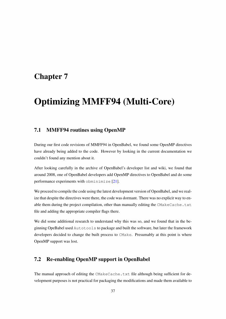
7.4 obconformer Speedup using Multi-Core Acceleration (OpenMP)
Next we will like to discuss multi-core performance for obconformer. We will first start
by showing the speedup plots of this tool sorted by the number of atoms (see Figure 7.3) and
again sorted by the number of rotatable bonds (see Figure 7.4). These two plots confirmed what
we already suspected from our initial application benchmarking, that is, obconformer is the
application that will most likely benefit the most from any parallelization strategy.
The figures also gave us some additional insights. In particular, that the size of the molecule
(number of atoms) is a stronger predictor of the speedup than the number of rotamers .
7.5 obconformerEfficiency using Multi-Core Acceleration (OpenMP)
The same suite of molecules (Bostrom) was used to generate efficiency plots for obconformer.
Again two different plots were created in one we colored individual molecules using their size
(see Figure 7.5) and in the other we colored them according to the number of rotatable bonds
(see Figure 7.6). This way we can appreciate that the efficiency of this parallelization strategy
is best for molecules having the largest number of atoms. We also see from the graph that the
number of rotamers is not a good predictor of the scaling efficiency we would achieve using
obconformer.

Chapter 7. Optimizing MMFF94 (Multi-Core) 41
0.5
1
1.5
2
2.5
3
3.5
4
1 2 3 4 5 6 7 8
Spe
edup
Number of Processes
Num
ber
of A
tom
s
18
23
26
3032
3739
43
48
52
55
61
65
74
FIGURE 7.3: obconformer speedup vs atoms.
0.5
1
1.5
2
2.5
3
3.5
4
1 2 3 4 5 6 7 8
Spe
edup
Number of Processes
Num
ber
of R
otor
s
1
2
3
4
5
6
7
8
11
FIGURE 7.4: obconformer speedup vs rotors.
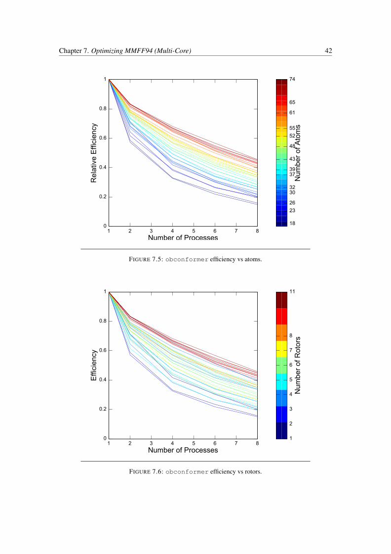
Chapter 7. Optimizing MMFF94 (Multi-Core) 42
0
0.2
0.4
0.6
0.8
1
1 2 3 4 5 6 7 8
Rel
ativ
e E
ffici
ency
Number of Processes
Num
ber
of A
tom
s
18
23
26
3032
3739
43
48
52
55
61
65
74
FIGURE 7.5: obconformer efficiency vs atoms.
0
0.2
0.4
0.6
0.8
1
1 2 3 4 5 6 7 8
Effi
cien
cy
Number of Processes
Num
ber
of R
otor
s
1
2
3
4
5
6
7
8
11
FIGURE 7.6: obconformer efficiency vs rotors.

Chapter 7. Optimizing MMFF94 (Multi-Core) 43
7.6 confab Speedup using Multi-Core Acceleration (OpenMP)
Finally we tested confab scaling using multi-core acceleration. This time we do also a mixed
plot, for both speedup and efficiency (see Figure 7.7).
0
0.2
0.4
0.6
0.8
1
0 2 4 6 8 10 12
Rel
ativ
e E
ffici
ency
Number of Processes
confab Efficiency (OpenMP)
18 atoms22 atoms23 atoms24 atoms26 atoms26 atoms27 atoms30 atoms31 atoms32 atoms33 atoms33 atoms37 atoms38 atoms39 atoms41 atoms43 atoms43 atoms
43 atoms47 atoms47 atoms48 atoms50 atoms52 atoms53 atoms53 atoms55 atoms59 atoms61 atoms64 atoms64 atoms65 atoms68 atoms68 atoms74 atoms
0.3
0.4
0.5
0.6
0.7
0.8
0.9
1
0 2 4 6 8 10 12
Spe
edup
Number of Processes
confab Speedup (OpenMP)
18 atoms22 atoms23 atoms24 atoms26 atoms26 atoms27 atoms30 atoms31 atoms32 atoms33 atoms33 atoms37 atoms38 atoms39 atoms41 atoms43 atoms43 atoms
43 atoms47 atoms47 atoms48 atoms50 atoms52 atoms53 atoms53 atoms55 atoms59 atoms61 atoms64 atoms64 atoms65 atoms68 atoms68 atoms74 atoms
FIGURE 7.7: confab speedup and efficiency.
Given the results that we got for conformational search with obconformer, the equivalent
results that we got from using multi-core acceleration with confab could appear somehow
intriguing. Effectively there is no speedup to be obtained, and in fact there is a performance
penalty we got from using multiple cores to run confab. The key to understand what is going
on is to understand the way confab works. confab does not make use of obminimize
to optimize the conformers, because it assumes each generated conformer is already unique,
and will directly evaluate its energy and discard it if the generated conformer is not within the
threshold specified by the user.
That is, confab purpose is to generate as many conformers as it can possibly found that satisfy
the energy threshold barrier specified by the user, and it will not perform a complete energy
evaluation (obminimize). It will only evaluate the changes from torsional and non-bonded
interactions.
Chapter 7. Optimizing MMFF94 (Multi-Core) 44
In conclusion the benefits from multi-core acceleration are best observed in obconformer,
but they are in fact a composition between performance gained when evaluating gradients in
obminimize and performance gains from parallelizing the complete forcefields energy func-
tion (obenergy).

Chapter 8
Optimizing MMFF94 (GPU)
8.1 Software Acceleration using GPU
The use of Graphics Processing Units (GPUs) for accelerating software is a trendy discussion
topic in the scientific computing community. We hear all the time about the fantastic perfor-
mance gains from taking this approach.
The problem strive in finding enough sources of parallelism within our code, for such an ap-
proach to be effective. Experts recommend; there must be thousands of threads running in
parallel on the GPU in order to get a speedup [22].
OpenBabel’s MMFF94 implementation barely uses more than a few hundred of threads simul-
taneously, so there is not a good forecast in this sense. Nevertheless we decided it would be
interesting to explore and learn more about GPU programming in the context of a real applica-
tion.
8.2 Heterogeneous Computing using OpenCL
It turns out there are several different approaches that can be used to program using the GPU.
The one most widely adopted is CUDA, the programming library and framework created by
Nvidia. In our case however we decided to use OpenCL, the reason being CUDA support is
restricted to Nvidia GPUs, while OpenCL is available for a larger number of platforms [4].
Also OpenCL headers, can be bundled and distributed together with OpenBabel, which is not
45
Chapter 8. Optimizing MMFF94 (GPU) 46
the case for CUDA. In addition, OpenCL is closer in spirit to OpenBabel which is perhaps the
most important reason we had to use it in our project.
OpenCL is equivalent to CUDA in the sense it is a very low level library that gives its users a
lot of control regarding how to manage computation using an heterogeneous architecture.
The way OpenCL works can be summarized into four steps:
1. The host (CPU) serializes the data that is sent to the device (GPU).
2. The code (kernel) that will be executed by the device is loaded by the host.
3. The host launches the kernel and waits for the device to complete its execution.
4. The data coming from the device is deserialized into the host memory.
As it is the case with every new technology, they were many subtleties to consider and a steep
learning curve to climb. Nonetheless, we were very interested in seeing if the promise of GPU
accelerated computing could be fulfilled for the MMFF94 implementation and motivated to try
the technology.
8.3 MMFF94 using GPU Architecture
We opt for a very simple architecture (see Figure 8.1) so that we can study the scaling behaviour
of the code using GPU, and come up later with refinements.
The idea was to separate the computation in two parts. The non-bonded terms, being the largest
in terms of number of independent calculations, were placed into the device, giving the rest of
the work to the host. The idea was to launch both partial computations simultaneously and in
this way overlap computation taking place in the host with the communication steps occurring
between both of them.
To minimize the performance penalties associated with compiling and loading the kernels these
are only read and compiled once for each architecture, and later they are stored in their binary
form together with the kernel source code.
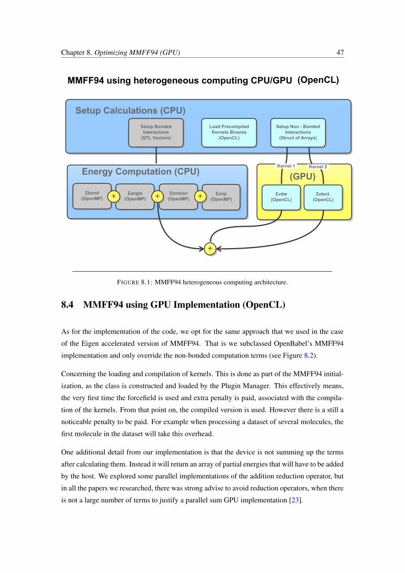
Chapter 8. Optimizing MMFF94 (GPU) 47
MMFF94 using heterogeneous computing CPU/GPU (OpenCL)
Setup BondedInteractions
(STL Vectors)
Setup Non - BondedInteractions
(Struct of Arrays)
Σvdw(OpenCL)
Σelect.(OpenCL)
Σbond(OpenMP)
Σangle(OpenMP)
Σtorsion(OpenMP)
Σoop(OpenMP)+ + +
Load PrecompiledKernels Binares
(OpenCL)
Setup Calculations (CPU)
Energy Computation (CPU) (GPU)
+
Kernel 1 Kernel 2
FIGURE 8.1: MMFF94 heterogeneous computing architecture.
8.4 MMFF94 using GPU Implementation (OpenCL)
As for the implementation of the code, we opt for the same approach that we used in the case
of the Eigen accelerated version of MMFF94. That is we subclassed OpenBabel’s MMFF94
implementation and only override the non-bonded computation terms (see Figure 8.2).
Concerning the loading and compilation of kernels. This is done as part of the MMFF94 initial-
ization, as the class is constructed and loaded by the Plugin Manager. This effectively means,
the very first time the forcefield is used and extra penalty is paid, associated with the compila-
tion of the kernels. From that point on, the compiled version is used. However there is a still a
noticeable penalty to be paid. For example when processing a dataset of several molecules, the
first molecule in the dataset will take this overhead.
One additional detail from our implementation is that the device is not summing up the terms
after calculating them. Instead it will return an array of partial energies that will have to be added
by the host. We explored some parallel implementations of the addition reduction operator, but
in all the papers we researched, there was strong advise to avoid reduction operators, when there
is not a large number of terms to justify a parallel sum GPU implementation [23].

Chapter 8. Optimizing MMFF94 (GPU) 48
OBPlugin
+ TypeID()+ MakeInstance()+ Init()+ GetID()
OBForceFieldMMFF94OpenCL
+ Setup(OBMol &mol)+ SetupGPU()+ Energy()+ E_VDW()+ E_Electrostatic()
Class Diagram - MMFF94 + OpenCL
implementsOBForceField
+ FindForceField(name : String)+ SetParameterFile()+ Setup(mol : OBMol)+ Energy(calculateGradients : bool)+ ConjugateGradients(steps,econv)+ VectorBondDerivative()+ VectorAngleDerivative()+ VectorTorsionDerivative()+ VectorSubtract()+ VectorAdd()+ VectorDivide()+ VectorMultiply()+ VectorNormalize()+ VectorDot()+ VectorCross()
OBForceFieldMMFF94
+ SetupCalculations()+ Setup(OBMol &mol)+ Energy()+ E_Bond()+ E_Angle()+ E_StrBnd()+ E_Torsion()+ E_OOP()+ E_VDW()+ E_Electrostratic()
OBMol
- bonds : Vector<OBBond>- atoms : Vector<OBAtom>
+ GetTitle()+ NumHvyAtoms()+ GetRotors()
OBBond
- parent : OBMol- begin : OBAtom- end : OBAtom
OBAtom
- bondList : Vector- coordinates : Vector- element : Integer- indexAtom : Integer
FIGURE 8.2: GPU enabled MMFF94 implementation class diagram.
8.5 MMFF94 acceleration using GPU Results
The first results that we obtained from using GPU acceleration were truly disappointing. The
execution time was dominated by the time spent in loading the kernels and communicating with
the GPU. The negative performance impact was of two orders of magnitude.
Results are however consistent with our initial findings. There is currently not enough paral-
lelism in OpenBabel’s MMFF94 implementation to consider offloading some computation to
the GPU. It remains to be seen what will happen if we try larger molecules (HMWs). There are
however two reasons that can be argued against the use of HMWs. The first is that the MMFF94
model has only be tested and recommended for relatively small molecules. The second being
larger molecules will put a toll on the system memory.

Chapter 8. Optimizing MMFF94 (GPU) 49
8.6 Accelerating MMFF94 Applications Perspectives
From our previous discussion is clear that OpenBabel’s MMFF94 implementation is not amenable
for GPU acceleration. However, there is still a couple of things we would have like to explore.
For example, changing the plugin mechanism. The proposal will be to create a pool of force-
fields, so that several molecules could be computed in parallel, instead of being pipelined.
The proposal will include avoiding the setup step for the non-bonded pairs and instead doing all
the computing using the GPU. Also as a way to give more work to the GPU, it will be desirable
to merge both: the electrostatic and van-der-Waals computations into a single larger one. An
additional advantage of avoiding the setup step, will be that no strong memory demands will
have to be enforced and we will in theory be able to treat larger molecules.
Chapter 9
Discussion of Results
In this work we explored the acceleration of OpenBabel’s forcefield implementation, and we
found that despite the function to be accelerated belongs to the category of ”embarrassingly
parallel” problems, its parallelization is not straightforward.
In particular we found OpenBabel’s current architecture limits the parallelization that can be
achieved. The reason being, that the plugin mechanism, responsible of loading the forcefields,
uses a singleton pattern to avoid more than one forcefield implementation being used at any
given time. This, composed with the fact that forcefields create memory structures specific for
each molecule, restricts them to be used for more than one molecule at a time.
Furthermore, the precomputing of energy terms, an optimization used in OpenBabel’s MMFF94
to reduce the time spent computing energy functions, have the side effect of limiting the size of
the molecules that can be treated using OpenBabel’s forcefields implementation.
Three different optimization approaches were taken during the course of this work. First, the
optimization for single core, that even thought, didn’t have the final expected results, was a good
first step to take, in order to familiarize with the MMFF94 model and OpenBabel’s implemen-
tation.
Second, the multi-core acceleration using OpenMP, which was the most straightforward and not
as thought demanding as the first and third one, but still was so far, the one giving us better
performance results when compared with the other two. The code to enable this optimization
has been contributed back to OpenBabel.
The third one, an attempt to use GPU computing to offload the computation of non-bonded
interactions. The implementation was successful, but the results were disappointing. We realize,
50
Chapter 9. Discussion of Results 51
that in order for such an approach to be used, a more drastic change in OpenBabel’s architecture
is needed.
Other possible optimization paths, like the optimization of Conjugate Gradient algorithm in
obminimize or Conformer Search algorithm in confab were not attempted because of time
limitations, and are left as future work directions.
Chapter 10
Conclusions
The present work main contribution was a better understanding of OpenBabel’s MMFF94 im-
plementation and its applications from a performance optimization perspective.
From the benchmarking of OpenBabel’s applications using MMFF94, we showed conformers
generation tools: confab and obconformer; to be the ones having the largest fraction of
work occurring in parallel, and therefore also the best candidates for parallelization.
We advised also OpenBabel’s developers community, to continue using and porting other por-
tions of the code to Eigen. Despite we didn’t achieve the performance improvements that we
were expecting, the Eigen port brought two other equally important benefits to the project: an
improved code readability and maintainability.
With respect to the use of OpenMP to enable performance, we would argue, it is still the fastest,
less disruptive strategy to chose as a first parallelization approach, especially considering the
widespread adoption of multi-core processors in research and academy.
As regarding the use of GPU to accelerate performance, our conclusion is that there should
be an strong motivation for it (use case), and proven sources of parallelism (e.g. a very large
simulation). The reason being GPU programming demands a large investment of time and
significant code refactoring. The last assertion is all the more true for object oriented codes
where computation is spread at several layers.
In conclusion, OpenBabel’s MMFF94 implementation is, according to the above expressed cri-
teria, not suitable for GPU acceleration.
52
Appendix A
MMFF94 Components
The MMFF94 as originally described in the article by Thomas A Halgren has two different
versions MMFF94 and MMFF94s. The difference between these two is on the selection of
parameters, but the force components used in both are the same. In this appendix only the
MMFF94 is described, but OpenBabel also supports the MMFF94s variant, in which case an
appropriate set of parameters is loaded, but the implementation is shared.
The MMFF94 considers seven different force components in its formulation, when summed
them up the energy of the molecule is obtained. The compact expression of MMFF94 is:
E =∑
Ebond +∑
Eangle +∑
Estretch +∑
Eoop +∑
Etorsion +∑
Evdw +∑
Eelect.
Next, each force contributions and the way to compute them is presented. Vectors appearing
in the equations are identified using bold face, for example FSi , to refer to the stretch force
exerted upon atom i. The MMFF94 empirical and derived parameters are shown in cursive. The
lower case subscripts i, j, k, l refer to the individual atoms of a molecule. Upper case subscripts
I, J,K,L are constants matching the atom type.
The force terms are derived by taking the negative gradient of the potential energy;
F = −∇V
53
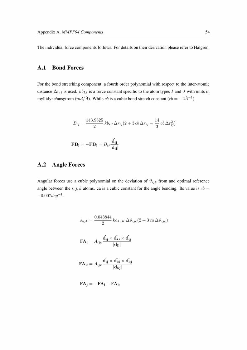
Appendix A. MMFF94 Components 54
The individual force components follows. For details on their derivation please refer to Halgren.
A.1 Bond Forces
For the bond stretching component, a fourth order polynomial with respect to the inter-atomic
distance ∆rij is used. kbIJ is a force constant specific to the atom types I and J with units in
myllidyne/ansgtrom (md/A). While cb is a cubic bond stretch constant (cb = −2A−1).
Bij =143.9325
2kbIJ ∆rij(2 + 3 cb∆rij −
14
3cb∆r2ij)
FBi = −FBj = Bijdij
|dij|
A.2 Angle Forces
Angular forces use a cubic polynomial on the deviation of ϑijk from and optimal reference
angle between the i, j, k atoms. ca is a cubic constant for the angle bending. Its value is cb =
−0.007deg−1.
Aijk =0.043844
2kaIJK ∆ϑijk(2 + 3 ca∆ϑijk)
FAi = Aijkdij × dki × dij
|dij|
FAk = Aijkdij × dki × dkj
|dkj|
FAj = −FAi − FAk

Appendix A. MMFF94 Components 55
A.3 Stretch Bend Forces
The stretch components considers both the deviation from the optimal distance and angle, for
the bond couples ij and jk and the angle ijk.
Sijk = −(2.51210)2 (ksIJK ∆rij + ksKJI ∆rkj) ∆ϑijk
FSi = Sijk ksIJKdij × dki × dij
|dij|
FSk = Sijk ksKJIdij × dki × dkj
|dkj|
FSj = −FSi − FSk
A.4 Torsional Forces
The torsion component depends on four atoms i, j, k, l. The extreme atoms i, l are two bond
distances apart from each other by the direct bonded couple j, k. As a result, they will exert a
torsional force on the bond between atoms j and k (the torsion angle φ).

Appendix A. MMFF94 Components 56
Tijkl = V1 sin(φ)− 2V2 sin(2φ) + 3V3 sin(3φ)
FTi = Tijkldij × djk
sin(φ)2 |dij|
FTl = Tijkldjk × dkl
sin(φ)2 |dkl|
FTj = FTi|dij|
(−cos(φ)) |djk|− 1− FTl
|dkl|(−cos(φ)) |djk|
FTk = −(FTi + FTj + FTl)
A.5 Out-of-Plane Forces
The out-of-plane component as its name says is used to determine the force component for
trigonal centers. χijk;l is known as the Wilson angle between the bond jl and the plane ijk.
koopIJK;L is a constant in function of the four atoms.

Appendix A. MMFF94 Components 57
Oijkl =0.043844χijk;l · koopIJK;L
cos(χijk;l)
FOi = Oijkldjk × djl − dji + djk cos(ϑijk) sin(χijk;l)/sin(ϑijk)
sin(ϑijk) |dji|
FOk = Oijkldjl × dji − djk + dji cos(ϑijk) sin(χijk;l)/sin(ϑijk)
sin(ϑijk) |djk|
FOl = Oijkldji × djl · sin−1(ϑijk)− djl sin(χijk;l)
|djl|
FOj = −(FOi + FOk + FOl)
A.6 Van-der-Waals Forces
This force term considers non-bonded interactions between atoms pairs. In order to be consid-
ered as a non-bonded interaction, atoms have to be separated by at least three bonds. εIJ is a
constant for the atom types IJ , Rij is the current distance between atomsIJ), and R∗IJ is the
optimal distance between these two atoms.
q =Rij
R∗IJ
Vij =εijR∗
IJ
(1.07
q + 0.07
)7( −7.84 q6
(q7 + 0.12)2+−7.84/(q7 + 0.12) + 14
q + 0.07
)
FVi = −FVj = Vij dij
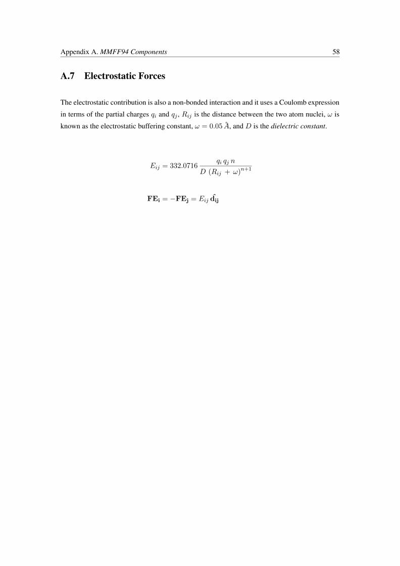
Appendix A. MMFF94 Components 58
A.7 Electrostatic Forces
The electrostatic contribution is also a non-bonded interaction and it uses a Coulomb expression
in terms of the partial charges qi and qj , Rij is the distance between the two atom nuclei, ω is
known as the electrostatic buffering constant, ω = 0.05 A, and D is the dielectric constant.
Eij = 332.0716qi qj n
D (Rij + ω)n+1
FEi = −FEj = Eij dij
Appendix B
Installing OpenBabel using MMFF94with OpenCL
The following set of instructions is provided in order to help the readers interested in trying the
OpenCL accelerated version of MMFF94 in OpenBabel. Instructions assume that the project
will be built using the sources available in the project’s public repository. The only two prerequi-
sites to successfully compile and build the program are the GNU C++ development environment
(g++, make) and CMake (version 2.4 or newer).
The source code can be checked out from a local repository at github.com using git:
$ git clone https://github.com/ovalerio/ocl_openbabel.git
In order to compile OpenBabel, you will need a recent version of CMake (version ≥ 2.4). To
find out which version of CMake is installed on your system, you can use the -v switch.
$ cmake -v
OpenBabel requires access to Eigen source code and header files. Eigen is a C++ template
library for matrix manipulation and linear algebra. OpenBabel uses version 3.x of Eigen.
You can get Eigen sources from the Eigen Project Website.
Eigen sources need to be unpacked and placed in a directory accessible to the user. In this
example we will download and extract Eigen in a directory directly under our home directory.
59
Appendix B. Installing OpenBabel using MMFF94 with OpenCL 60
$ wget http://bitbucket.org/eigen/eigen/get/3.1.1.zip
$ unzip 3.1.1.zip
$ mv eigen-eigen-43d9075b23ef eigen
In case you’re not familiar with CMake. The important thing to know about it, is that CMake
will take care of generating the Makefiles for the project in a cross-platform compatible way.
CMake recommends that builds are performed out-of-source. This is to avoid mixing your
build directory with the project source files. For this to happen, you first need to be inside the
directory where OpenBabel sources have been downloaded. Inside this directory, you create a
directory called build and from inside this directory run CMake. The commands to do this are
the following:
$ cd ocl_openbabel/
$ mkdir build
$ cd build
$ cmake -DEIGEN3_INCLUDE_DIR=˜/eigen -DENABLE_OPENMP=TRUE \
-DCMAKE_INSTALL_PREFIX=˜/openbabel -DCMAKE_BUILD_TYPE=RELEASE \
-DOPENCL_INCLUDE_DIRS=/cuda/4.2/cuda/include -DMINIMAL_BUILD=TRUE \
-DENABLE_TESTS=OFF ..
$ make; make install
You will notice from the parameter list to CMake above that we are enabling both OpenMP and
OpenCL support. Another switch is used to indicate where the Eigen sources can be found.
A couple of other flags are set to indicate CMake that we want it to create a minimal build in
release mode. Finally, we also set a flag with the location where we want the binaries of the
program to be installed.
Assuming everything went well up to this point, you will end up with OpenBabel being installed
and ready to run on your computer. If you look inside the bin folder, you will find several
programs that have been compiled as command line utilities. The source for this programs is
inside a directory called part1. There are three main programs obenergyx, obminimizex
and obconformerx.
To run any of them, you will need a dataset of molecules. Also in the project folder, you will
find a folder containing some datasets that we have been using to test Confab. For example, let’s
say you might want to try the bostrom.sdf dataset. Then you will have to do the following:

Appendix B. Installing OpenBabel using MMFF94 with OpenCL 61
˜/ocl_openbabel/build$ cd ..
˜/ocl_openbabel$ cd dataset/
˜/ocl_openbabel/dataset$ ls
bostrom.sdf optimized-borodina-subset.sdf forcefield.sdf
˜/ocl_openbabel/dataset$ obminimizex -ff MMFF94GPU \
-h bostrom.sdf
Apart from minimizing the molecules in the bostrom.sdf dataset, the program will generate
files with runtime statistics for memory use and computation time. The files will be named as
<program name> runstats <forcefield> t<proc>.mat. For example, the output
of obminimize using MMFF94GPU and 4 threads will be written in:
obminimize runstats mmff94gpu t4.mat.

Appendix C
Installing Confab using OpenMP code
The following set of instructions is provided in order to help the readers interested in trying
the OpenMP accelerated version of Confab. The instructions assume that the project will be
built using the sources available in the project’s public repository. The only two prerequisites to
successfully compile and build the program are the GNU C++ development environment (g++,
make) and CMake (version 2.4 or newer).
The source code can be checked out from a public repository at github.com using git:
$ git clone https://github.com/ovalerio/omp_confab.git
In order to compile Confab from the sources once you have download them, you will need a
recent version of CMake (version ≥ 2.4). To find out which version of CMake is installed on
your system, you can use the -v switch.
$ cmake -v
Confab also requires access to Eigen source code and header files. Eigen is a linear algebra
template library similar to Blas, that allows micro-optimization for single-threaded software.
Eigen is now in version 3.x but presently Confab only works with version 2.x of Eigen.
You can get Eigen from the Eigen Project Website.
You will need to unpack it and place it somewhere around your environment, so that later on
CMake can refer to it. In this example we will download and extract Eigen in a directory directly
under our home directory.
62

Appendix C. Installing Confab using OpenMP code 63
$ wget http://bitbucket.org/eigen/eigen/get/2.0.17.zip
$ unzip 2.0.17.zip
$ mv eigen-eigen-b23437e61a07 eigen
In case you’re not familiar with CMake. The important thing to know about it is that CMake
will take care of generating the Makefiles for the project in a cross-platform compatible way.
CMake recommends that builds are performed out-of-source. This is to avoid mixing your build
directory with the project source files. For this to happen, you first need to be inside the directory
where Confab sources have been downloaded. Inside this directory, you create a directory called
build and from inside this directory run CMake. The commands to do this are the following:
$ cd omp_confab/
$ mkdir build
$ cd build
$ cmake -DEIGEN2_INCLUDE_DIR=˜/eigen -DENABLE_OPENMP=TRUE \
-DCMAKE_INSTALL_PREFIX=˜/confab ..
$ make; make install
You will notice from the parameter list given to CMake above that we are enabling OpenMP
support. Another switch is used to indicate where the Eigen sources can be found. Finally, we
also set a flag with the location where we want the binaries of the program to be installed.
Assuming everything went well up to this point, you will end up with Confab being installed
and ready to run on your computer. If you look inside the bin folder, you will find several
programs that have been compiled as command line utilities. The source for this programs
is inside a directory called parallel. There are three main programs obenergy mmff94,
obminimize mmff94 and confab mmff94.
To run any of them, you will need a dataset of molecules. Also in the project folder, you will
find a folder containing some datasets that we have been using to test Confab. For example, let’s
say you might want to try the bostrom.sdf dataset. Then you will have to do the following:
˜/omp_confab/build$ cd ..
˜/omp_confab$ cd dataset/
˜/omp_confab/dataset$ ls
bostrom.sdf optimized-borodina-subset.sdf forcefield.sdf
˜/omp_confab/dataset$ confab_mmff94 -osdf \
bostrom.sdf /dev/null
Appendix C. Installing Confab using OpenMP code 64
You might notice we are not saving the conformers. Instead, we choose to redirect the output
to /dev/null because conformers files tend to be quite chunky and use a lot of disk space.
Besides, conformers files are not useful for benchmarking purposes. The file we are interested
in is the one called confab runstats.dat, which, as its name implies, contains execution
statistics for the confab tool.
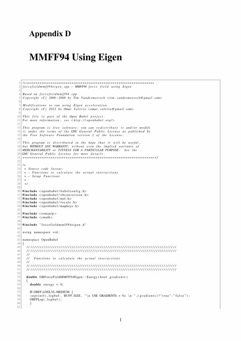
Appendix D
MMFF94 Using Eigen
1 /∗ ∗∗∗∗∗∗∗∗∗∗∗∗∗∗∗∗∗∗∗∗∗∗∗∗∗∗∗∗∗∗∗∗∗∗∗∗∗∗∗∗∗∗∗∗∗∗∗∗∗∗∗∗∗∗∗∗∗∗∗∗∗∗∗∗∗∗∗∗2 f o r c e f i e l d m m f f 9 4 e i g e n . cpp − MMFF94 f o r c e f i e l d u s i n g Eigen34 Based on f o r c e f i e l d m m f f 9 4 . cpp5 C o p y r i g h t (C) 2006−2008 by Tim Vandermeersch <t i m . vandermeersch@gmail . com>67 M o d i f i c a t i o n s t o run u s i n g Eigen a c c e l e r a t i o n8 C o p y r i g h t (C) 2012 by Omar V a l e r i o <omar . v a l e r i o @ g m a i l . com>9
10 T h i s f i l e i s p a r t o f t h e Open Babel p r o j e c t .11 For more i n f o r m a t i o n , s e e <h t t p : / / openbabe l . org />1213 T h i s program i s f r e e s o f t w a r e ; you can r e d i s t r i b u t e i t and / or m od i f y14 i t under t h e t e r m s o f t h e GNU Genera l P u b l i c L i c e n s e as p u b l i s h e d by15 t h e Free S o f t w a r e Founda t ion v e r s i o n 2 o f t h e L i c e n s e .1617 T h i s program i s d i s t r i b u t e d i n t h e hope t h a t i t w i l l be u s e f u l ,18 b u t WITHOUT ANY WARRANTY; w i t h o u t even t h e i m p l i e d w a rr a n t y o f19 MERCHANTABILITY or FITNESS FOR A PARTICULAR PURPOSE . See t h e20 GNU Genera l P u b l i c L i c e n s e f o r more d e t a i l s .21 ∗∗∗∗∗∗∗∗∗∗∗∗∗∗∗∗∗∗∗∗∗∗∗∗∗∗∗∗∗∗∗∗∗∗∗∗∗∗∗∗∗∗∗∗∗∗∗∗∗∗∗∗∗∗∗∗∗∗∗∗∗∗∗∗∗∗∗∗∗∗ ∗ /2223 /∗24 ∗ Source code l a y o u t :25 ∗ − F u n c t i o n s t o c a l c u l a t e t h e a c t u a l i n t e r a c t i o n s26 ∗ − S e t u p F u n c t i o n s27 ∗28 ∗ /2930 # i n c l u d e <o p e n b a b e l / b a b e l c o n f i g . h>31 # i n c l u d e <o p e n b a b e l / o b c o n v e r s i o n . h>32 # i n c l u d e <o p e n b a b e l / mol . h>33 # i n c l u d e <o p e n b a b e l / l o c a l e . h>34 # i n c l u d e <o p e n b a b e l / mapkeys . h>3536 # i n c l u d e <iomanip>37 # i n c l u d e <cmath>3839 # i n c l u d e ” f o r c e f i e l d m m f f 9 4 e i g e n . h ”4041 u s i n g namespace s t d ;4243 namespace OpenBabel44 {45 / / / / / / / / / / / / / / / / / / / / / / / / / / / / / / / / / / / / / / / / / / / / / / / / / / / / / / / / / / / / / / / / / / / / / / / / / / / / / / / /46 / / / / / / / / / / / / / / / / / / / / / / / / / / / / / / / / / / / / / / / / / / / / / / / / / / / / / / / / / / / / / / / / / / / / / / / / / / / / / / / /47 / /48 / / F u n c t i o n s t o c a l c u l a t e t h e a c t u a l i n t e r a c t i o n s49 / /50 / / / / / / / / / / / / / / / / / / / / / / / / / / / / / / / / / / / / / / / / / / / / / / / / / / / / / / / / / / / / / / / / / / / / / / / / / / / / / / / /51 / / / / / / / / / / / / / / / / / / / / / / / / / / / / / / / / / / / / / / / / / / / / / / / / / / / / / / / / / / / / / / / / / / / / / / / / / / / / / / / /5253 double OBForceFieldMMFF94Eigen : : Energy ( b oo l g r a d i e n t s )54 {55 double e ne r g y = 0 ;5657 IF OBFF LOGLVL MEDIUM {58 s n p r i n t f ( l o g b u f , BUFF SIZE , ”\n USE GRADIENTS = %s \n ” , ( g r a d i e n t s ) ? ” t r u e ” : ” f a l s e ” ) ;59 OBFFLog ( l o g b u f ) ;60 }61
1
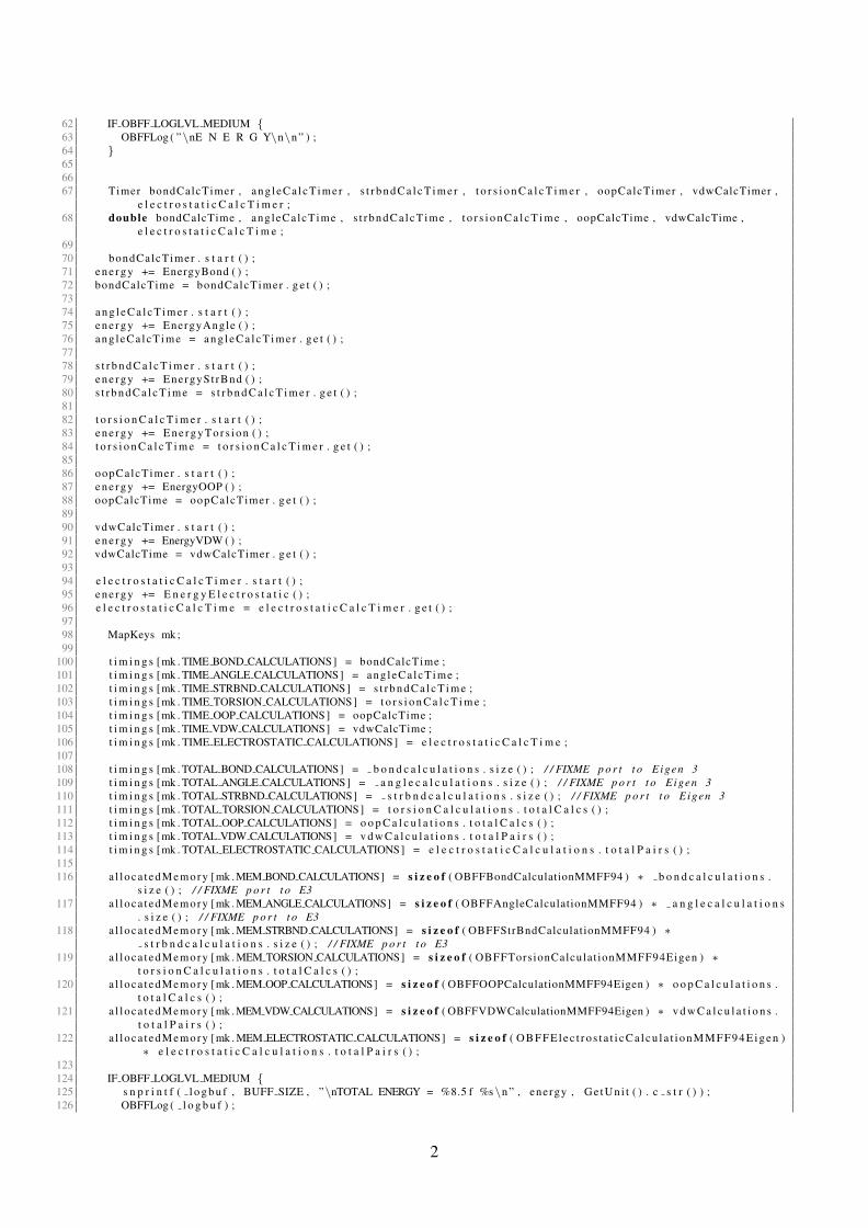
62 IF OBFF LOGLVL MEDIUM {63 OBFFLog ( ”\nE N E R G Y\n\n ” ) ;64 }656667 Timer bondCalcTimer , ang leCa lcT imer , s t r b n d C a l c T i m e r , t o r s i o n C a l c T i m e r , oopCalcTimer , vdwCalcTimer ,
e l e c t r o s t a t i c C a l c T i m e r ;68 double bondCalcTime , angleCalcTime , s t rbndCa lcT ime , t o r s i o n C a l c T i m e , oopCalcTime , vdwCalcTime ,
e l e c t r o s t a t i c C a l c T i m e ;6970 bondCalcTimer . s t a r t ( ) ;71 en e r g y += EnergyBond ( ) ;72 bondCalcTime = bondCalcTimer . g e t ( ) ;7374 a n g l e C a l c T i m e r . s t a r t ( ) ;75 en e r g y += EnergyAngle ( ) ;76 ang leCa lcT ime = a n g l e C a l c T i m e r . g e t ( ) ;7778 s t r b n d C a l c T i m e r . s t a r t ( ) ;79 en e r g y += EnergySt rBnd ( ) ;80 s t r b n d C a l c T i m e = s t r b n d C a l c T i m e r . g e t ( ) ;8182 t o r s i o n C a l c T i m e r . s t a r t ( ) ;83 en e r g y += E n e r g y T o r s i o n ( ) ;84 t o r s i o n C a l c T i m e = t o r s i o n C a l c T i m e r . g e t ( ) ;8586 oopCalcTimer . s t a r t ( ) ;87 en e r g y += EnergyOOP ( ) ;88 oopCalcTime = oopCalcTimer . g e t ( ) ;8990 vdwCalcTimer . s t a r t ( ) ;91 en e r g y += EnergyVDW ( ) ;92 vdwCalcTime = vdwCalcTimer . g e t ( ) ;9394 e l e c t r o s t a t i c C a l c T i m e r . s t a r t ( ) ;95 en e r g y += E n e r g y E l e c t r o s t a t i c ( ) ;96 e l e c t r o s t a t i c C a l c T i m e = e l e c t r o s t a t i c C a l c T i m e r . g e t ( ) ;9798 MapKeys mk ;99
100 t i m i n g s [mk . TIME BOND CALCULATIONS] = bondCalcTime ;101 t i m i n g s [mk . TIME ANGLE CALCULATIONS] = ang leCa lcT ime ;102 t i m i n g s [mk . TIME STRBND CALCULATIONS] = s t r b n d C a l c T i m e ;103 t i m i n g s [mk . TIME TORSION CALCULATIONS ] = t o r s i o n C a l c T i m e ;104 t i m i n g s [mk . TIME OOP CALCULATIONS] = oopCalcTime ;105 t i m i n g s [mk . TIME VDW CALCULATIONS] = vdwCalcTime ;106 t i m i n g s [mk . TIME ELECTROSTATIC CALCULATIONS ] = e l e c t r o s t a t i c C a l c T i m e ;107108 t i m i n g s [mk . TOTAL BOND CALCULATIONS] = b o n d c a l c u l a t i o n s . s i z e ( ) ; / / FIXME p o r t t o Eigen 3109 t i m i n g s [mk . TOTAL ANGLE CALCULATIONS] = a n g l e c a l c u l a t i o n s . s i z e ( ) ; / / FIXME p o r t t o Eigen 3110 t i m i n g s [mk . TOTAL STRBND CALCULATIONS] = s t r b n d c a l c u l a t i o n s . s i z e ( ) ; / / FIXME p o r t t o Eigen 3111 t i m i n g s [mk . TOTAL TORSION CALCULATIONS] = t o r s i o n C a l c u l a t i o n s . t o t a l C a l c s ( ) ;112 t i m i n g s [mk . TOTAL OOP CALCULATIONS] = o o p C a l c u l a t i o n s . t o t a l C a l c s ( ) ;113 t i m i n g s [mk . TOTAL VDW CALCULATIONS] = v d w C a l c u l a t i o n s . t o t a l P a i r s ( ) ;114 t i m i n g s [mk . TOTAL ELECTROSTATIC CALCULATIONS] = e l e c t r o s t a t i c C a l c u l a t i o n s . t o t a l P a i r s ( ) ;115116 a l loca t edMemory [mk . MEM BOND CALCULATIONS] = s i z e o f ( OBFFBondCalculationMMFF94 ) ∗ b o n d c a l c u l a t i o n s .
s i z e ( ) ; / / FIXME p o r t t o E3117 a l loca t edMemory [mk . MEM ANGLE CALCULATIONS] = s i z e o f ( OBFFAngleCalculationMMFF94 ) ∗ a n g l e c a l c u l a t i o n s
. s i z e ( ) ; / / FIXME p o r t t o E3118 a l loca t edMemory [mk . MEM STRBND CALCULATIONS] = s i z e o f ( OBFFStrBndCalculationMMFF94 ) ∗
s t r b n d c a l c u l a t i o n s . s i z e ( ) ; / / FIXME p o r t t o E3119 a l loca t edMemory [mk . MEM TORSION CALCULATIONS] = s i z e o f ( OBFFTorsionCalculat ionMMFF94Eigen ) ∗
t o r s i o n C a l c u l a t i o n s . t o t a l C a l c s ( ) ;120 a l loca t edMemory [mk . MEM OOP CALCULATIONS] = s i z e o f ( OBFFOOPCalculationMMFF94Eigen ) ∗ o o p C a l c u l a t i o n s .
t o t a l C a l c s ( ) ;121 a l loca t edMemory [mk .MEM VDW CALCULATIONS] = s i z e o f ( OBFFVDWCalculationMMFF94Eigen ) ∗ v d w C a l c u l a t i o n s .
t o t a l P a i r s ( ) ;122 a l loca t edMemory [mk . MEM ELECTROSTATIC CALCULATIONS] = s i z e o f ( O B F F E l e c t r o s t a t i c C a l c u l a t i o n M M F F 9 4 E i g e n )
∗ e l e c t r o s t a t i c C a l c u l a t i o n s . t o t a l P a i r s ( ) ;123124 IF OBFF LOGLVL MEDIUM {125 s n p r i n t f ( l o g b u f , BUFF SIZE , ”\nTOTAL ENERGY = %8.5 f %s\n ” , energy , Ge tUn i t ( ) . c s t r ( ) ) ;126 OBFFLog ( l o g b u f ) ;
2
127 }128129 re turn e ne r g y ;130 }131132133 / /134 / / MMFF p a r t I − page 494135 / /136 / / k b i j 7137 / / E B i j = 143 .9325 −−−−−−− /\ r i j ˆ 2 (1 + cs /\ r i j + −−−− cs ˆ2 r i j ˆ 2 )138 / / 2 12139 / /140 / / k b i j f o r c e c o n s t a n t ( md / A )141 / /142 / / /\ r i j r i j − r 0 i j ( A )143 / /144 / / c s c u b i c s t r e t c h c o n s t a n t = −2 Aˆ(−1)145 / /146 double OBForceFieldMMFF94Eigen : : EnergyBond ( ) {147148 double e ne rg y = 0 . 0 ;149150 s t d : : v e c t o r<OBFFBondCalculationMMFF94 > : : i t e r a t o r i t e r a t o r ;151152 s t d : : v e c t o r<Eigen : : Vector3d> posAVector ;153 s t d : : v e c t o r<Eigen : : Vector3d> posBVector ;154 s t d : : v e c t o r<double> r 0 V e c t o r ;155 s t d : : v e c t o r<double> kbVec to r ;156157 Eigen : : Vec to r3d posA , posB ;158159 f o r ( i t e r a t o r = b o n d c a l c u l a t i o n s . b e g i n ( ) ; i t e r a t o r != b o n d c a l c u l a t i o n s . end ( ) ; i t e r a t o r ++){160 posA << (∗ i t e r a t o r ) . p o s a [ 0 ] , (∗ i t e r a t o r ) . p o s a [ 1 ] , (∗ i t e r a t o r ) . p o s a [ 2 ] ;161 posAVector . p u s h b a c k ( posA ) ;162 posB << (∗ i t e r a t o r ) . p o s b [ 0 ] , (∗ i t e r a t o r ) . pos b [ 1 ] , (∗ i t e r a t o r ) . p os b [ 2 ] ;163 posBVector . p u s h b a c k ( posB ) ;164 r 0 V e c t o r . p u s h b a c k ( (∗ i t e r a t o r ) . r0 ) ;165 kbVec to r . p u s h b a c k ( (∗ i t e r a t o r ) . kb ) ;166 } / / f o r ( b o n d C a l c u l a t i o n s )167168 Eigen : : Vec to r3d rAB ;169170 double r0 , kb ;171 double d e l t a , d e l t a s q ;172173 f o r ( i n t i ndx = 0 ; indx < b o n d c a l c u l a t i o n s . s i z e ( ) ; i ndx ++){174 posA = posAVector [ i ndx ] ;175 posB = posBVector [ i nd x ] ;176 r0 = r 0 V e c t o r [ i ndx ] ;177 kb = kbVec to r [ i ndx ] ;178179 / / c a l c u l a t e t h e bond v e c t o r s and d e t e r m i n e i t s l e n g t h ( d i s t a n c e )180 rAB = posA − posB ;181 d e l t a = rAB . norm ( ) − r0 ;182 d e l t a s q = pow ( d e l t a , 2 ) ;183184 e n e r g y += kb ∗ d e l t a s q ∗ ( 1 . 0 − 2 . 0 ∗ d e l t a + 7 . 0 / 3 . 0 ∗ d e l t a s q ) ;185186 } / / f o r ( b o n d C a l c u l a t i o n s )187188 en e r g y = 143 .9325 ∗ 0 . 5 ∗ e ne rg y ;189190 re turn e ne rg y ;191192 }193194 / /195 / / MMFF p a r t I − page 495196 / /197 / / k a i j k198 / / E A i j k = 0.438449325 −−−−−−−− /\0 i j k ˆ2 (1 + cs /\0 i j k )199 / / 2200 / /
3
201 / / k a i j k f o r c e c o n s t a n t ( md A / rad ˆ 2 )202 / /203 / / /\0 i j k 0 i j k − 00 i j k ( d e g r e e s )204 / /205 / / c s c u b i c bend c o n s t a n t = −0.007 degˆ−1 = −0.4 rad ˆ−1206 / /207 double OBForceFieldMMFF94Eigen : : EnergyAngle ( ) {208209 double e ne rg y = 0 . 0 ;210211 s t d : : v e c t o r<OBFFAngleCalculationMMFF94 > : : i t e r a t o r i t e r a t o r ;212213 s t d : : v e c t o r<Eigen : : Vector3d> posAVector ;214 s t d : : v e c t o r<Eigen : : Vector3d> posBVector ;215 s t d : : v e c t o r<Eigen : : Vector3d> posCVector ;216 s t d : : v e c t o r<double> t h e t a 0 V e c t o r ;217 s t d : : v e c t o r<double> k a V e c t o r ;218 s t d : : v e c t o r<bool> l i n e a r V e c t o r ;219220 Eigen : : Vec to r3d posA , posB , posC ;221222 f o r ( i t e r a t o r = a n g l e c a l c u l a t i o n s . b e g i n ( ) ; i t e r a t o r != a n g l e c a l c u l a t i o n s . end ( ) ; i t e r a t o r ++){223 posA << (∗ i t e r a t o r ) . p o s a [ 0 ] , (∗ i t e r a t o r ) . p o s a [ 1 ] , (∗ i t e r a t o r ) . p o s a [ 2 ] ;224 posAVector . p u s h b a c k ( posA ) ;225 posB << (∗ i t e r a t o r ) . p o s b [ 0 ] , (∗ i t e r a t o r ) . pos b [ 1 ] , (∗ i t e r a t o r ) . p os b [ 2 ] ;226 posBVector . p u s h b a c k ( posB ) ;227 posC << (∗ i t e r a t o r ) . p o s c [ 0 ] , (∗ i t e r a t o r ) . p o s c [ 1 ] , (∗ i t e r a t o r ) . p o s c [ 2 ] ;228 posCVector . p u s h b a c k ( posC ) ;229 t h e t a 0 V e c t o r . p u s h b a c k ( (∗ i t e r a t o r ) . t h e t a 0 ) ;230 k a V e c t o r . p u s h b a c k ( (∗ i t e r a t o r ) . ka ) ;231 l i n e a r V e c t o r . p u s h b a c k ( (∗ i t e r a t o r ) . l i n e a r ) ;232 } / / f o r ( a n g l e C a l c u l a t i o n s )233234 Eigen : : Vec to r3d rAB , rBC ;235236 double t h e t a , c o s t h e t a ;237 double t h e t a 0 , d e l t a t h e t a ;238 double ka ;239 boo l l i n e a r ;240241 f o r ( i n t i ndx = 0 ; indx < a n g l e c a l c u l a t i o n s . s i z e ( ) ; i ndx ++){242 posA = posAVector [ i ndx ] ;243 posB = posBVector [ i nd x ] ;244 posC = posCVector [ i nd x ] ;245 t h e t a 0 = t h e t a 0 V e c t o r [ i ndx ] ;246 ka = k a V e c t o r [ i ndx ] ;247 l i n e a r = l i n e a r V e c t o r [ i ndx ] ;248249 / / c a l c u l a t e t h e bond v e c t o r s be tween t h e t h r e e atoms250 rAB = posA − posB ;251 rBC = posC − posB ;252253 / / pe r fo rm i n p l a c e n o r m a l i z a t i o n o f t h e v e c t o r s254 rAB . n o r m a l i z e ( ) ;255 rBC . n o r m a l i z e ( ) ;256257 / / c a l c u l a t e t h e c o s i n e t h e t a and o b t a i n t h e t a258 c o s t h e t a = rAB . d o t ( rBC ) ;259 t h e t a = RAD TO DEG ∗ a cos ( c o s t h e t a ) ;260261 d e l t a t h e t a = t h e t a − t h e t a 0 ;262263 i f ( l i n e a r ) {264 en e r g y += 143 .9325 ∗ ka ∗ ( 1 . 0 + cos ( t h e t a ∗ DEG TO RAD) ) ;265 } e l s e {266 en e r g y += 0 .043844 ∗ 0 . 5 ∗ ka ∗ pow ( d e l t a t h e t a , 2 ) ∗ ( 1 . 0 − 0 . 007 ∗ d e l t a t h e t a ) ;267 }268269 } / / f o r ( a n g l e C a l c u l a t i o n s )270271 re turn e ne rg y ;272273 }274
4
275276 / /277 / / MMFF p a r t I − page 495278 / /279 / / E B A i j k = 2 .51210 ( k b a i j k /\ r i j + k b a k j i /\ r k j ) /\0 i j k280 / /281 / / k b a i j k f o r c e c o n s t a n t ( md / rad )282 / / k b a k j i f o r c e c o n s t a n t ( md / rad )283 / /284 / / /\ r x x s e e above285 / / /\0 i j k s e e above286 / /287 double OBForceFieldMMFF94Eigen : : EnergySt rBnd ( ) {288289 double e ne rg y = 0 . 0 ;290291 s t d : : v e c t o r<OBFFStrBndCalculationMMFF94 > : : i t e r a t o r i t e r a t o r ;292293 s t d : : v e c t o r<Eigen : : Vector3d> posAVector ;294 s t d : : v e c t o r<Eigen : : Vector3d> posBVector ;295 s t d : : v e c t o r<Eigen : : Vector3d> posCVector ;296 s t d : : v e c t o r<double> t h e t a 0 V e c t o r ;297 s t d : : v e c t o r<double> r a b 0 V e c t o r ;298 s t d : : v e c t o r<double> r b c 0 V e c t o r ;299 s t d : : v e c t o r<double> kbaABCVector ;300 s t d : : v e c t o r<double> kbaCBAVector ;301302 Eigen : : Vec to r3d posA , posB , posC ;303304 f o r ( i t e r a t o r = s t r b n d c a l c u l a t i o n s . b e g i n ( ) ; i t e r a t o r != s t r b n d c a l c u l a t i o n s . end ( ) ; i t e r a t o r ++){305 posA << (∗ i t e r a t o r ) . p o s a [ 0 ] , (∗ i t e r a t o r ) . p o s a [ 1 ] , (∗ i t e r a t o r ) . p o s a [ 2 ] ;306 posAVector . p u s h b a c k ( posA ) ;307 posB << (∗ i t e r a t o r ) . p o s b [ 0 ] , (∗ i t e r a t o r ) . pos b [ 1 ] , (∗ i t e r a t o r ) . p os b [ 2 ] ;308 posBVector . p u s h b a c k ( posB ) ;309 posC << (∗ i t e r a t o r ) . p o s c [ 0 ] , (∗ i t e r a t o r ) . p o s c [ 1 ] , (∗ i t e r a t o r ) . p o s c [ 2 ] ;310 posCVector . p u s h b a c k ( posC ) ;311 t h e t a 0 V e c t o r . p u s h b a c k ( (∗ i t e r a t o r ) . t h e t a 0 ) ;312 r a b 0 V e c t o r . p u s h b a c k ( (∗ i t e r a t o r ) . r ab0 ) ;313 r b c 0 V e c t o r . p u s h b a c k ( (∗ i t e r a t o r ) . r bc0 ) ;314 kbaABCVector . p u s h b a c k ( (∗ i t e r a t o r ) . kbaABC ) ;315 kbaCBAVector . p u s h b a c k ( (∗ i t e r a t o r ) . kbaCBA ) ;316 } / / f o r ( s t r b n d C a l c u l a t i o n s )317318 Eigen : : Vec to r3d rAB , rBC ;319 double lenAB , lenBC ;320321 double c o s t h e t a , t h e t a ;322 double d e l t a t h e t a , d e l t a r a b , d e l t a r b c ;323 double t h e t a 0 , rab0 , rbc0 ;324 double f a c t o r , kbaABC , kbaCBA ;325326 f o r ( i n t i ndx = 0 ; indx < s t r b n d c a l c u l a t i o n s . s i z e ( ) ; i nd x ++){327 posA = posAVector [ i ndx ] ;328 posB = posBVector [ i nd x ] ;329 posC = posCVector [ i nd x ] ;330 t h e t a 0 = t h e t a 0 V e c t o r [ i ndx ] ;331 rab0 = r a b 0 V e c t o r [ i ndx ] ;332 rbc0 = r b c 0 V e c t o r [ i ndx ] ;333 kbaABC = kbaABCVector [ i ndx ] ;334 kbaCBA = kbaCBAVector [ i ndx ] ;335336 / / c a l c u l a t e t h e bond v e c t o r s be tween t h e t h r e e atoms337 rAB = posA − posB ;338 rBC = posC − posB ;339340 / / c a l c u l a t e v e c t o r l e n g t h s f o r t h e bond v e c t o r s341 lenAB = rAB . norm ( ) ;342 lenBC = rBC . norm ( ) ;343344 / / pe r fo rm i n p l a c e n o r m a l i z a t i o n o f t h e v e c t o r s345 rAB . n o r m a l i z e ( ) ;346 rBC . n o r m a l i z e ( ) ;347348 / / c a l c u l a t e t h e c o s i n e t h e t a and o b t a i n t h e t a
5
349 c o s t h e t a = rAB . d o t ( rBC ) ;350 t h e t a = RAD TO DEG ∗ a cos ( c o s t h e t a ) ;351352 d e l t a t h e t a = t h e t a − t h e t a 0 ;353 d e l t a r a b = lenAB − r ab0 ;354 d e l t a r b c = lenBC − r bc0 ;355 f a c t o r = kbaABC ∗ d e l t a r a b + kbaCBA ∗ d e l t a r b c ;356357 e n e r g y += f a c t o r ∗ d e l t a t h e t a ;358359 } / / f o r ( s t r b n d C a l c u l a t i o n s )360361 en e r g y = 2 .51210 ∗ e ne r g y ;362363 re turn e ne rg y ;364365 }366367368 / /369 / / MMFF p a r t I − page 495370 / /371 / / E T i j k l = 0 . 5 ( V1 (1 + cos (0 i j k l ) ) + V2 (1 − cos (2 0 i j k l ) ) + V3 (1 + cos (3 0 i j k l ) ) )372 / /373 / / V1 f o r c e c o n s t a n t ( md / rad )374 / / V2 f o r c e c o n s t a n t ( md / rad )375 / / V3 f o r c e c o n s t a n t ( md / rad )376 / /377 / / 0 i j k l t o r s i o n a n g l e ( d e g r e e s )378 / /379 double OBForceFieldMMFF94Eigen : : E n e r g y T o r s i o n ( ) {380 double e ne rg y = 0 . 0 ;381382 Eigen : : Vec to r3d posA , posB , posC , posD , v e l ;383384 Eigen : : Vec to r3d rAB , rBC , rCD ;385 Eigen : : Vec to r3d nR , nS , nT ;386 double lenAB , lenBC , lenCD ;387388 double d1 , d2 , t o r ;389 double cos1 , cos2 , cos3 ;390 Eigen : : Vec to r3d p h i ;391392 f o r ( i n t i ndx = 0 ; indx < t o r s i o n C a l c u l a t i o n s . t o t a l C a l c s ( ) ; i ndx ++){393 posA = t o r s i o n C a l c u l a t i o n s . posAVector [ i ndx ] ;394 posB = t o r s i o n C a l c u l a t i o n s . posBVector [ i ndx ] ;395 posC = t o r s i o n C a l c u l a t i o n s . posCVector [ i ndx ] ;396 posD = t o r s i o n C a l c u l a t i o n s . posDVector [ i ndx ] ;397 v e l = t o r s i o n C a l c u l a t i o n s . v e l o c i t y V e c t o r [ i ndx ] ;398399 / / c a l c u l a t e bond v e c t o r s be tween t h e t h r e e atoms400 rAB = posB − posA ;401 rBC = posC − posB ;402 rCD = posD − posC ;403404 / / c a l c u l a t e v e c t o r l e n g t h s f o r t h e bond v e c t o r s405 lenAB = rAB . norm ( ) ;406 lenBC = rBC . norm ( ) ;407 lenCD = rCD . norm ( ) ;408409 / / pe r fo rm i n p l a c e n o r m a l i z a t i o n o f t h e v e c t o r s410 rAB . n o r m a l i z e ( ) ;411 rBC . n o r m a l i z e ( ) ;412 rCD . n o r m a l i z e ( ) ;413414 / / c a l c u l a t e t h e normal v e c t o r s o f t h e t h r e e p l a n e s415 nR = rAB . c r o s s ( rBC ) ;416 nS = rBC . c r o s s ( rCD ) ;417 nT = nR . c r o s s ( nS ) ;418419 / / c a l c u l a t e d1 , d2 , t o r420 d1 = nT . d o t ( rBC ) ;421 d2 = nR . d o t ( nS ) ;422 t o r = RAD TO DEG ∗ a t a n 2 ( d1 , d2 ) ;
6
423424 cos1 = cos (DEG TO RAD ∗ 1 ∗ t o r ) ;425 cos2 = cos (DEG TO RAD ∗ 2 ∗ t o r ) ;426 cos3 = cos (DEG TO RAD ∗ 3 ∗ t o r ) ;427428 p h i ( 0 ) = 1 . 0 + cos1 ;429 p h i ( 1 ) = 1 . 0 − cos2 ;430 p h i ( 2 ) = 1 . 0 + cos3 ;431432 e n e r g y += v e l . d o t ( p h i ) ;433434 } / / f o r ( t o r s i o n C a l c u l a t i o n s )435436 en e r g y = 0 . 5 ∗ e ne r g y ;437438 re turn e ne rg y ;439 }440441442 / / / /443 / / a / /444 / / \ / /445 / / b−−−d p l a n e = a−b−c / /446 / / / / /447 / / c / /448 / / / /449 double OBForceFieldMMFF94Eigen : : EnergyOOP ( ) {450 double e ne r g y = 0 . 0 ;451452 Eigen : : Vec to r3d posA , posB , posC , posD ;453 Eigen : : Vec to r3d rBA , rBC , rBD ;454 Eigen : : Vec to r3d nABC, nCBD, nABD;455 double ang le , normBA , normBC , normBD ;456457 double t h e t a , c o s t h e t a , s i n t h e t a , s i n d l ;458 double koop ;459460 / / The Out o f Plane term compute was o r i g i n a l l y adap ted from Andreas Moll d i s s e r t a t i o n on BALLView461 / / h t t p : / / s c i d o k . s u l b . uni−s a a r l a n d . de / v o l l t e x t e / 2 0 0 7 / 1 3 2 5 / p d f / D i s s e r t a t i o n 1 5 4 4 M o l l A n d r 2 0 0 7 . p d f462 #pragma omp p a r a l l e l f o r d e f a u l t ( none ) \463 p r i v a t e ( posA , posB , posC , posD , rBA , rBC , rBD , nABC, nCBD, nABD, ang le , normBA , normBC , normBD , \464 t h e t a , c o s t h e t a , s i n t h e t a , s i n d l , koop ) r e d u c t i o n (+ : e n e r gy )465 f o r ( i n t i ndx = 0 ; indx < o o p C a l c u l a t i o n s . t o t a l C a l c s ( ) ; i ndx ++){466 posA = o o p C a l c u l a t i o n s . posAVector [ i ndx ] ;467 posB = o o p C a l c u l a t i o n s . posBVector [ i ndx ] ;468 posC = o o p C a l c u l a t i o n s . posCVector [ i ndx ] ;469 posD = o o p C a l c u l a t i o n s . posDVector [ i ndx ] ;470 koop = o o p C a l c u l a t i o n s . koopVec tor [ i ndx ] ;471472 / / c a l c u l a t e bond v e c t o r s from c e n t r a l atom t o o u t e r atoms473 rBA = posA − posB ;474 rBC = posC − posB ;475 rBD = posD − posB ;476477 / / c a l c u l a t e v e c t o r l e n g t h s f o r t h e bond v e c t o r s478 normBA = rBA . norm ( ) ;479 normBC = rBC . norm ( ) ;480 normBD = rBD . norm ( ) ;481482 / / pe r fo rm i n p l a c e n o r m a l i z a t i o n o f t h e v e c t o r s483 rBA . n o r m a l i z e ( ) ;484 rBC . n o r m a l i z e ( ) ;485 rBD . n o r m a l i z e ( ) ;486487 / / c a l c u l a t e t h e normal v e c t o r s o f t h e t h r e e p l a n e s488 nABC = rBA . c r o s s ( rBC ) ;489 nCBD = rBC . c r o s s ( rBD ) ;490 nABD = rBD . c r o s s ( rBA ) ;491492 / / t h e t a i s t h e a n g l e be tween rBA and rBC493 c o s t h e t a = rBA . d o t ( rBC ) ;494 t h e t a = ac o s ( c o s t h e t a ) ;495 s i n t h e t a = s i n ( t h e t a ) ;496
7

497 s i n d l = nABC . d o t ( rBD ) / s i n t h e t a ;498499 / / t h e w i l s o n a n g l e i s t h e a s i n500 a n g l e = RAD TO DEG ∗ a s i n ( s i n d l ) ;501502 / / i f ( ! i s f i n i t e ( a n g l e ) )503 / / a n g l e = 0 . 0 ; / / doesn ’ t e x p l a i n why GetAngle i s r e t u r n i n g NaN b u t s o l v e s i t f o r us ;504505 e n e r g y += koop ∗ pow ( ang le , 2 ) ;506507 } / / f o r ( v d w c a l c u l a t i o n s )508509 en e r g y = 0 .043844 ∗ 0 . 5 ∗ e ne rg y ;510511 re turn e ne rg y ;512 }513514515 / / / Van der Waals non−bonded i n t e r a c t i o n c o n t r i b u t i o n516 double OBForceFieldMMFF94Eigen : : EnergyVDW ( ) {517 double e ne r g y = 0 . 0 ;518519 Eigen : : Vec to r3d posA , posB ;520 Eigen : : Vec to r3d di f fAB ;521 double RAB, RAB7 ;522 double rab , rab7 , qq ;523 double erep , e rep7 , e a t t r ;524 double e p s i l o n ;525526 #pragma omp p a r a l l e l f o r d e f a u l t ( none ) \527 p r i v a t e ( posA , posB , diffAB , RAB, RAB7, rab , rab7 , qq , \528 erep , e rep7 , e a t t r , e p s i l o n ) r e d u c t i o n (+ : e ne rg y )529 f o r ( i n t i ndx = 0 ; indx < v d w C a l c u l a t i o n s . t o t a l P a i r s ( ) ; i ndx ++){530 posA = v d w C a l c u l a t i o n s . posAVector [ i ndx ] ;531 posB = v d w C a l c u l a t i o n s . posBVector [ i ndx ] ;532 di f fAB = posA − posB ;533 r a b = di f fAB . norm ( ) ; / / d i s t a n c e be tween atoms534 rab7 = pow ( rab , 7 ) ;535 RAB = v d w C a l c u l a t i o n s . RABVector [ i n dx ] ;536 RAB7 = v d w C a l c u l a t i o n s . RAB7Vector [ i ndx ] ; ;537 e p s i l o n = v d w C a l c u l a t i o n s . e p s i l o n V e c t o r [ i ndx ] ;538 e r e p = ( 1 . 0 7 ∗ RAB) / ( r a b + 0 . 0 7 ∗ RAB) ;539 e r e p 7 = pow ( erep , 7 ) ;540 e a t t r = ( ( ( 1 . 1 2 ∗ RAB7) / ( r ab7 + 0 . 1 2 ∗ RAB7) ) − 2 . 0 ) ;541 e n e r g y += e p s i l o n ∗ e r e p 7 ∗ e a t t r ;542 } / / f o r ( v d w c a l c u l a t i o n s )543544 re turn e ne rg y ;545 }546547548 / / E l e c t r o s t a t i c c o n t r i b u t i o n549 double OBForceFieldMMFF94Eigen : : E n e r g y E l e c t r o s t a t i c ( ) {550 double e ne rg y = 0 . 0 ;551552 Eigen : : Vec to r3d posA , posB ;553 Eigen : : Vec to r3d di f fAB ;554 double dis tanceAB , qq ;555556 #pragma omp p a r a l l e l f o r d e f a u l t ( none ) \557 p r i v a t e ( posA , posB , d is tanceAB , diffAB , qq ) r e d u c t i o n (+ : e ne r g y )558 f o r ( i n t i ndx = 0 ; indx < e l e c t r o s t a t i c C a l c u l a t i o n s . t o t a l P a i r s ( ) ; i ndx ++){559 posA = e l e c t r o s t a t i c C a l c u l a t i o n s . posAVector [ i ndx ] ;560 posB = e l e c t r o s t a t i c C a l c u l a t i o n s . posBVector [ i ndx ] ;561 di f fAB = posA − posB ;562 d i s t anceAB = dif fAB . norm ( ) ;563 qq = e l e c t r o s t a t i c C a l c u l a t i o n s . qqVec to r [ i ndx ] ;564 e n e r g y += qq / ( d i s t anceAB + 0 . 0 5 ) ; / / 0 . 0 5 t o a v o i d z e r o d i v i s i o n565 } / / f o r ( e l e c t r o s t a t i c )566567 re turn e ne rg y ;568 }569570
8

571 / /572 / / OBForceFieldMMFF94Eigen member f u n c t i o n s573 / /574 / / ∗∗∗∗∗∗∗∗∗∗∗∗∗∗∗∗∗∗∗∗∗∗∗∗∗∗∗∗∗∗∗∗∗∗∗∗∗∗∗∗∗∗∗∗∗∗∗575 / / Make a g l o b a l i n s t a n c e576 OBForceFieldMMFF94Eigen theForceFie ldMMFF94Eigen ( ”MMFF94Eigen” , f a l s e ) ;577 OBForceFieldMMFF94Eigen theForceFie ldMMFF94sEigen ( ”MMFF94sEigen” , f a l s e ) ;578 / / ∗∗∗∗∗∗∗∗∗∗∗∗∗∗∗∗∗∗∗∗∗∗∗∗∗∗∗∗∗∗∗∗∗∗∗∗∗∗∗∗∗∗∗∗∗∗∗579580 OBForceFieldMMFF94Eigen : : ˜ OBForceFieldMMFF94Eigen ( )581 {582 }583584 OBForceFieldMMFF94Eigen &OBForceFieldMMFF94Eigen : : o p e r a t o r =( OBForceFieldMMFF94Eigen &s r c )585 {586 mol = s r c . mol ;587 i n i t = s r c . i n i t ;588 re turn ∗ t h i s ;589 }590591592 boo l OBForceFieldMMFF94Eigen : : S e t u p C a l c u l a t i o n s ( )593 {594 IF OBFF LOGLVL LOW595 OBFFLog ( ”\nS E T T I N G U P C A L C U L A T I O N S\n\n ” ) ;596597 boo l g r a d i e n t s = f a l s e ; / / FIXME t h i s parame te r w i l l come as an argument598599 # i f n d e f EIGEN VECTORIZE600 s t d : : c o u t << ”ATTENTION! VECTORIZATION SUPPORT WAS DISABLED FOR EIGEN . ” << s t d : : e n d l ;601 # e n d i f602603 b oo l s e t u p ;604 s e t u p = S e t u p B o n d C a l c u l a t i o n s ( g r a d i e n t s ) ;605 s e t u p &= S e t u p A n g l e A n d S t r B n d C a l c u l a t i o n s ( g r a d i e n t s ) ;606 s e t u p &= S e t u p T o r s i o n C a l c u l a t i o n s ( g r a d i e n t s ) ;607 s e t u p &= S e t u p O O P C a l c u l a t i o n s ( g r a d i e n t s ) ;608 s e t u p &= SetupVDWCalcula t ions ( g r a d i e n t s ) ;609 s e t u p &= S e t u p E l e c t r o s t a t i c C a l c u l a t i o n s ( g r a d i e n t s ) ;610611 re turn s e t u p ;612 }613614 / /615 / / Bond C a l c u l a t i o n s616 / /617 / / no ” s t e p−down” p r o c e d u r e618 / / MMFF p a r t V − page 625 ( e m p i r i c a l r u l e )619 / /620 boo l OBForceFieldMMFF94Eigen : : S e t u p B o n d C a l c u l a t i o n s ( boo l g r a d i e n t s )621 {622 OBFFParameter ∗ p a r a m e t e r ;623 OBAtom ∗a , ∗b , ∗c , ∗d ;624 i n t t y p e a , t y p e b , t y p e c , t y p e d ;625 b oo l found ;626 i n t o r d e r ;627628 IF OBFF LOGLVL LOW629 OBFFLog ( ”SETTING UP BOND CALCULATIONS . . . \ n ” ) ;630631 OBFFBondCalculationMMFF94 b o n d c a l c ;632 i n t bond type ;633634 b o n d c a l c u l a t i o n s . c l e a r ( ) ;635636 FOR BONDS OF MOL( bond , mol ) {637 a = bond−>GetBeginAtom ( ) ;638 b = bond−>GetEndAtom ( ) ;639640 / / s k i p t h i s bond i f t h e atoms are i g n o r e d641 i f ( c o n s t r a i n t s . I s I g n o r e d ( a−>Get Idx ( ) ) | | c o n s t r a i n t s . I s I g n o r e d ( b−>Get Idx ( ) ) )642 c o n t i nu e ;643644 / / i f t h e r e are any groups s p e c i f i e d , check i f t h e two bond atoms are i n a s i n g l e i n t r a G r o u p
9

645 i f ( HasGroups ( ) ) {646 boo l va l i dBond = f a l s e ;647 f o r ( unsigned i n t i =0 ; i < i n t r a G r o u p . s i z e ( ) ; ++ i ) {648 i f ( i n t r a G r o u p [ i ] . B i t I s O n ( a−>Get Idx ( ) ) && i n t r a G r o u p [ i ] . B i t I s O n ( b−>Get Idx ( ) ) ) {649 va l i dBond = t r u e ;650 break ;651 }652 }653 i f ( ! va l i dBond )654 c o n t i nu e ;655 }656657 bond type = GetBondType ( a , b ) ;658659 p a r a m e t e r = GetTypedParameter2Atom ( bondtype , a t o i ( a−>GetType ( ) ) , a t o i ( b−>GetType ( ) ) , f f b o n d p a r a m s
) ; / / f rom mmffbond . par660 i f ( p a r a m e t e r == NULL) {661 p a r a m e t e r = GetParameter2Atom ( a−>GetAtomicNum ( ) , b−>GetAtomicNum ( ) , f f b n d k p a r a m s ) ; / / f rom
mmffbndk . par − e m p e r i c a l r u l e s662 i f ( p a r a m e t e r == NULL) {663 IF OBFF LOGLVL LOW {664 / / T h i s s h o u l d n e v e r happen665 s n p r i n t f ( l o g b u f , BUFF SIZE , ” COULD NOT FIND PARAMETERS FOR BOND %d−%d ( IDX ) . . . \ n ” , a−>
Get Idx ( ) , b−>Get Idx ( ) ) ;666 OBFFLog ( l o g b u f ) ;667 }668 re turn f a l s e ;669 } e l s e {670 IF OBFF LOGLVL LOW {671 s n p r i n t f ( l o g b u f , BUFF SIZE , ” USING EMPIRICAL RULE FOR BOND STRETCHING %d−%d ( IDX ) . . . \ n ” ,
a−>Get Idx ( ) , b−>Get Idx ( ) ) ;672 OBFFLog ( l o g b u f ) ;673 }674675 double r r , r r 2 , r r 4 , r r 6 ;676 b o n d c a l c . a = a ;677 b o n d c a l c . b = b ;678 b o n d c a l c . r0 = GetRuleBondLength ( a , b ) ;679680 r r = p a r a m e t e r−> d p a r [ 0 ] / b o n d c a l c . r0 ; / / parameter−> dpa r [ 0 ] = r0−r e f681 r r 2 = r r ∗ r r ;682 r r 4 = r r 2 ∗ r r 2 ;683 r r 6 = r r 4 ∗ r r 2 ;684685 b o n d c a l c . kb = p a r a m e t e r−> d p a r [ 1 ] ∗ r r 6 ; / / parameter−> dp a r [ 1 ] = kb−r e f686 b o n d c a l c . b t = bond type ;687 b o n d c a l c . S e t u p P o i n t e r s ( ) ;688689 b o n d c a l c u l a t i o n s . p u s h b a c k ( b o n d c a l c ) ;690 }691 } e l s e {692 b o n d c a l c . a = a ;693 b o n d c a l c . b = b ;694 b o n d c a l c . kb = p a r a m e t e r−> d p a r [ 0 ] ;695 b o n d c a l c . r0 = p a r a m e t e r−> d p a r [ 1 ] ;696 b o n d c a l c . b t = bond type ;697 b o n d c a l c . S e t u p P o i n t e r s ( ) ;698699 b o n d c a l c u l a t i o n s . p u s h b a c k ( b o n d c a l c ) ;700 }701 }702703 re turn t r u e ; / / no pr op er r e t u r n v a l u e ! !704 }705706 / /707 / / Angle C a l c u l a t i o n s708 / /709 / / MMFF p a r t I − page 513 (” s t e p−down” prodedure )710 / / MMFF p a r t I − page 519 ( r e f e r e n c e 68 i s a c t u a l l y a f o o t n o t e )711 / / MMFF p a r t V − page 627 ( e m p i r i c a l r u l e )712 / /713 / / F i r s t t r y and f i n d an e x a c t match , i f t h i s f a i l s , s t e p down u s i n g t h e e q u i v a l e n c e s from mmf fde f .
par
10

714 / / f i v e−s t a g e p r o t o c o l : 1−1−1, 2−2−2, 3−2−3, 4−2−4, 5−2−5715 / / I f t h i s f a i l s , use e m p i r i c a l r u l e s716 / / S i n c e 1−1−1 = 2−2−2, we w i l l o n l y t r y 1−1−1 b e f o r e go ing t o 3−2−3717 / /718 / / S t r e t c h−Bend C a l c u l a t i o n s719 / /720 boo l OBForceFieldMMFF94Eigen : : S e t u p A n g l e A n d S t r B n d C a l c u l a t i o n s ( boo l g r a d i e n t s )721 {722 OBFFParameter ∗ p a r a m e t e r ;723 OBAtom ∗a , ∗b , ∗c , ∗d ;724 i n t t y p e a , t y p e b , t y p e c , t y p e d ;725 b oo l found ;726 i n t o r d e r ;727728 IF OBFF LOGLVL LOW729 OBFFLog ( ”SETTING UP ANGLE & STRETCH−BEND CALCULATIONS . . . \ n ” ) ;730731 OBFFAngleCalculationMMFF94 a n g l e c a l c ;732 OBFFStrBndCalculationMMFF94 s t r b n d c a l c ;733 i n t a n g l e t y p e , s t r b n d t y p e , bondtype1 , bond type2 ;734735 a n g l e c a l c u l a t i o n s . c l e a r ( ) ;736 s t r b n d c a l c u l a t i o n s . c l e a r ( ) ;737738 FOR ANGLES OF MOL( ang le , mol ) {739 b = mol . GetAtom ( (∗ a n g l e ) [ 0 ] + 1 ) ;740 a = mol . GetAtom ( (∗ a n g l e ) [ 1 ] + 1 ) ;741 c = mol . GetAtom ( (∗ a n g l e ) [ 2 ] + 1 ) ;742743 t y p e a = a t o i ( a−>GetType ( ) ) ;744 t y p e b = a t o i ( b−>GetType ( ) ) ;745 t y p e c = a t o i ( c−>GetType ( ) ) ;746747 / / s k i p t h i s a n g l e i f t h e atoms are i g n o r e d748 i f ( c o n s t r a i n t s . I s I g n o r e d ( a−>Get Idx ( ) ) | | c o n s t r a i n t s . I s I g n o r e d ( b−>Get Idx ( ) ) | | c o n s t r a i n t s .
I s I g n o r e d ( c−>Get Idx ( ) ) )749 c o n t i nu e ;750751 / / i f t h e r e are any groups s p e c i f i e d , check i f t h e t h r e e a n g l e atoms are i n a s i n g l e i n t r a G r o u p752 i f ( HasGroups ( ) ) {753 boo l v a l i d A n g l e = f a l s e ;754 f o r ( unsigned i n t i =0 ; i < i n t r a G r o u p . s i z e ( ) ; ++ i ) {755 i f ( i n t r a G r o u p [ i ] . B i t I s O n ( a−>Get Idx ( ) ) && i n t r a G r o u p [ i ] . B i t I s O n ( b−>Get Idx ( ) ) &&756 i n t r a G r o u p [ i ] . B i t I s O n ( c−>Get Idx ( ) ) ) {757 v a l i d A n g l e = t r u e ;758 break ;759 }760 }761 i f ( ! v a l i d A n g l e )762 c o n t i nu e ;763 }764765 a n g l e t y p e = GetAngleType ( a , b , c ) ;766 s t r b n d t y p e = GetStrBndType ( a , b , c ) ;767 bond type1 = GetBondType ( a , b ) ;768 bond type2 = GetBondType ( b , c ) ;769770 i f ( HasLinSe t ( t y p e b ) ) {771 a n g l e c a l c . l i n e a r = t r u e ;772 } e l s e {773 a n g l e c a l c . l i n e a r = f a l s e ;774 }775776 / / t r y e x a c t match777 p a r a m e t e r = GetTypedParameter3Atom ( a n g l e t y p e , t y p e a , t y p e b , t y p e c , f f a n g l e p a r a m s ) ;778 i f ( p a r a m e t e r == NULL) / / t r y 3−2−3779 p a r a m e t e r = GetTypedParameter3Atom ( a n g l e t y p e , EqLvl3 ( t y p e a ) , t y p e b , EqLvl3 ( t y p e c ) ,
f f a n g l e p a r a m s ) ;780 i f ( p a r a m e t e r == NULL) / / t r y 4−2−4781 p a r a m e t e r = GetTypedParameter3Atom ( a n g l e t y p e , EqLvl4 ( t y p e a ) , t y p e b , EqLvl4 ( t y p e c ) ,
f f a n g l e p a r a m s ) ;782 i f ( p a r a m e t e r == NULL) / / t r y 5−2−5783 p a r a m e t e r = GetTypedParameter3Atom ( a n g l e t y p e , EqLvl5 ( t y p e a ) , t y p e b , EqLvl5 ( t y p e c ) ,
f f a n g l e p a r a m s ) ;
11
784785 i f ( p a r a m e t e r ) {786 a n g l e c a l c . ka = p a r a m e t e r−> d p a r [ 0 ] ;787 a n g l e c a l c . t h e t a 0 = p a r a m e t e r−> d p a r [ 1 ] ;788 s t r b n d c a l c . t h e t a 0 = p a r a m e t e r−> d p a r [ 1 ] ; / / ∗∗789 } e l s e {790 IF OBFF LOGLVL LOW {791 s n p r i n t f ( l o g b u f , BUFF SIZE , ” USING DEFAULT ANGLE FOR %d−%d−%d ( IDX ) . . . \ n ” , a−>Get Idx ( ) , b
−>Get Idx ( ) , c−>Get Idx ( ) ) ;792 s n p r i n t f ( l o g b u f , BUFF SIZE , ” USING EMPIRICAL RULE FOR ANGLE BENDING %d−%d−%d ( IDX ) . . . \ n ” ,
a−>Get Idx ( ) , b−>Get Idx ( ) , c−>Get Idx ( ) ) ;793 OBFFLog ( l o g b u f ) ;794 }795796 a n g l e c a l c . ka = 0 . 0 ;797 a n g l e c a l c . t h e t a 0 = 1 2 0 . 0 ;798799 i f ( GetCrd ( t y p e b ) == 4)800 a n g l e c a l c . t h e t a 0 = 1 0 9 . 4 5 ;801802 i f ( ( GetCrd ( t y p e b ) == 2) && b−>IsOxygen ( ) )803 a n g l e c a l c . t h e t a 0 = 1 0 5 . 0 ;804805 i f ( b−>GetAtomicNum ( ) > 10)806 a n g l e c a l c . t h e t a 0 = 9 5 . 0 ;807808 i f ( HasLinSe t ( t y p e b ) )809 a n g l e c a l c . t h e t a 0 = 1 8 0 . 0 ;810811 i f ( ( GetCrd ( t y p e b ) == 3) && ( GetVal ( t y p e b ) == 3) && ! GetMltb ( t y p e b ) ) {812 i f ( b−>I s N i t r o g e n ( ) ) {813 a n g l e c a l c . t h e t a 0 = 1 0 7 . 0 ;814 } e l s e {815 a n g l e c a l c . t h e t a 0 = 9 2 . 0 ;816 }817 }818819 i f ( a−>I s I n R i n g S i z e ( 3 ) && b−>I s I n R i n g S i z e ( 3 ) && c−>I s I n R i n g S i z e ( 3 ) && IsInSameRing ( a , c ) )820 a n g l e c a l c . t h e t a 0 = 6 0 . 0 ;821822 i f ( a−>I s I n R i n g S i z e ( 4 ) && b−>I s I n R i n g S i z e ( 4 ) && c−>I s I n R i n g S i z e ( 4 ) && IsInSameRing ( a , c ) )823 a n g l e c a l c . t h e t a 0 = 9 0 . 0 ;824825 s t r b n d c a l c . t h e t a 0 = a n g l e c a l c . t h e t a 0 ; / / ∗∗826 }827828 / / e m p i r i c a l r u l e f o r 0−b−0 and s t a n d a r d a n g l e s829 i f ( a n g l e c a l c . ka == 0 . 0 ) {830 IF OBFF LOGLVL LOW {831 s n p r i n t f ( l o g b u f , BUFF SIZE , ” USING EMPIRICAL RULE FOR ANGLE BENDING FORCE CONSTANT %d−%d−%
d ( IDX ) . . . \ n ” , a−>Get Idx ( ) , b−>Get Idx ( ) , c−>Get Idx ( ) ) ;832 OBFFLog ( l o g b u f ) ;833 }834835 double be ta , Za , Zc , Cb , r0ab , r0bc , t h e t a , t h e t a 2 , D, r r , r r 2 ;836 Za = GetZParam ( a ) ;837 Cb = GetCParam ( b ) ; / / F i xed t y p o −− PR#2741658838 Zc = GetZParam ( c ) ;839840 r0ab = GetBondLength ( a , b ) ;841 r0bc = GetBondLength ( b , c ) ;842 r r = r0ab + r0bc ;843 r r 2 = r r ∗ r r ;844 D = ( r0ab − r 0bc ) / r r 2 ;845846 t h e t a = a n g l e c a l c . t h e t a 0 ;847 t h e t a 2 = t h e t a ∗ t h e t a ;848849 b e t a = 1 . 7 5 ;850 i f ( a−>I s I n R i n g S i z e ( 4 ) && b−>I s I n R i n g S i z e ( 4 ) && c−>I s I n R i n g S i z e ( 4 ) && IsInSameRing ( a , c ) )851 b e t a = 0 . 8 5 ∗ b e t a ;852 i f ( a−>I s I n R i n g S i z e ( 3 ) && b−>I s I n R i n g S i z e ( 3 ) && c−>I s I n R i n g S i z e ( 3 ) && IsInSameRing ( a , c ) )853 b e t a = 0 . 0 5 ∗ b e t a ;854
12

855 / / The ta2 i s i n Degrees ˆ 2 , b u t p a r a m e t e r s are e x p e c t i n g r a d i a n s856 / / PR#2741669857 a n g l e c a l c . ka = ( b e t a ∗ Za ∗ Cb ∗ Zc ∗ exp(−2 ∗ D) ) / ( r r ∗ t h e t a 2 ∗ DEG TO RAD ∗ DEG TO RAD) ;858 }859860 a n g l e c a l c . a = a ;861 a n g l e c a l c . b = b ;862 a n g l e c a l c . c = c ;863 a n g l e c a l c . a t = a n g l e t y p e ;864865 a n g l e c a l c . S e t u p P o i n t e r s ( ) ;866 a n g l e c a l c u l a t i o n s . p u s h b a c k ( a n g l e c a l c ) ;867868 i f ( a n g l e c a l c . l i n e a r )869 c o n t i nu e ;870871 p a r a m e t e r = GetTypedParameter3Atom ( s t r b n d t y p e , t y p e a , t y p e b , t y p e c , f f s t r b n d p a r a m s ) ;872 i f ( p a r a m e t e r == NULL) {873 i n t rowa , rowb , rowc ;874875 rowa = GetElementRow ( a ) ;876 rowb = GetElementRow ( b ) ;877 rowc = GetElementRow ( c ) ;878879 p a r a m e t e r = GetParameter3Atom ( rowa , rowb , rowc , f f d f s b p a r a m s ) ;880881 i f ( p a r a m e t e r == NULL) {882 / / T h i s s h o u l d n e v e r happen883 IF OBFF LOGLVL LOW {884 s n p r i n t f ( l o g b u f , BUFF SIZE , ” COULD NOT FIND PARAMETERS FOR STRETCH−BEND %d−%d−%d ( IDX )
. . . \ n ” , a−>Get Idx ( ) , b−>Get Idx ( ) , c−>Get Idx ( ) ) ;885 OBFFLog ( l o g b u f ) ;886 }887 re turn f a l s e ;888 }889890 i f ( rowa == p a r a m e t e r−>a ) {891 s t r b n d c a l c . kbaABC = p a r a m e t e r−> d p a r [ 0 ] ;892 s t r b n d c a l c . kbaCBA = p a r a m e t e r−> d p a r [ 1 ] ;893 } e l s e {894 s t r b n d c a l c . kbaABC = p a r a m e t e r−> d p a r [ 1 ] ;895 s t r b n d c a l c . kbaCBA = p a r a m e t e r−> d p a r [ 0 ] ;896 }897 } e l s e {898 i f ( t y p e a == p a r a m e t e r−>a ) {899 s t r b n d c a l c . kbaABC = p a r a m e t e r−> d p a r [ 0 ] ;900 s t r b n d c a l c . kbaCBA = p a r a m e t e r−> d p a r [ 1 ] ;901 } e l s e {902 s t r b n d c a l c . kbaABC = p a r a m e t e r−> d p a r [ 1 ] ;903 s t r b n d c a l c . kbaCBA = p a r a m e t e r−> d p a r [ 0 ] ;904 }905 }906907 s t r b n d c a l c . r ab0 = GetBondLength ( a , b ) ;908 s t r b n d c a l c . rb c0 = GetBondLength ( b , c ) ;909 s t r b n d c a l c . a = a ;910 s t r b n d c a l c . b = b ;911 s t r b n d c a l c . c = c ;912 s t r b n d c a l c . s b t = s t r b n d t y p e ;913 s t r b n d c a l c . S e t u p P o i n t e r s ( ) ;914915 s t r b n d c a l c u l a t i o n s . p u s h b a c k ( s t r b n d c a l c ) ;916917 }918919 re turn t r u e ; / / FIXME here s h o u l d r e t u r n s o m e t h i n g m e a n i n g f u l or d e c l a r e method as v o i d920 }921922 / /923 / / T o r s i o n C a l c u l a t i o n s924 / /925 / / MMFF p a r t I − page 513 (” s t e p−down” prodedure )926 / / MMFF p a r t I − page 519 ( r e f e r e n c e 68 i s a c t u a l l y a f o o t n o t e )927 / / MMFF p a r t IV − page 631 ( e m p i r i c a l r u l e )
13
928 / /929 / / F i r s t t r y and f i n d an e x a c t match , i f t h i s f a i l s , s t e p down u s i n g t h e e q u i v a l e n c e s from mmf fde f .
par930 / / f i v e−s t a g e p r o t o c o l : 1−1−1−1, 2−2−2−2, 3−2−2−5, 5−2−2−3, 5−2−2−5931 / / I f t h i s f a i l s , use e m p i r i c a l r u l e s932 / / S i n c e 1−1−1−1 = 2−2−2−2, we w i l l o n l y t r y 1−1−1−1 b e f o r e go ing t o 3−2−2−5933 / /934 boo l OBForceFieldMMFF94Eigen : : S e t u p T o r s i o n C a l c u l a t i o n s ( boo l g r a d i e n t s )935 {936 OBFFParameter ∗ p a r a m e t e r ;937 OBAtom ∗a , ∗b , ∗c , ∗d ;938 i n t t y p e a , t y p e b , t y p e c , t y p e d ;939 b oo l found ;940 i n t o r d e r ;941942 IF OBFF LOGLVL LOW943 OBFFLog ( ”SETTING UP TORSION CALCULATIONS . . . \ n ” ) ;944945 i n t t o r s i o n t y p e ;946947 t o r s i o n C a l c u l a t i o n s . r e s e t ( ) ;948 double ∗pos a , ∗pos b , ∗pos c , ∗ pos d ;949 Eigen : : Vec to r3d v e l o c i t y ;950951 FOR TORSIONS OF MOL ( t , mol ) {952 a = mol . GetAtom ( (∗ t ) [ 0 ] + 1 ) ;953 b = mol . GetAtom ( (∗ t ) [ 1 ] + 1 ) ;954 c = mol . GetAtom ( (∗ t ) [ 2 ] + 1 ) ;955 d = mol . GetAtom ( (∗ t ) [ 3 ] + 1 ) ;956957 t y p e a = a t o i ( a−>GetType ( ) ) ;958 t y p e b = a t o i ( b−>GetType ( ) ) ;959 t y p e c = a t o i ( c−>GetType ( ) ) ;960 t y p e d = a t o i ( d−>GetType ( ) ) ;961962 / / s k i p t h i s t o r s i o n i f t h e atoms are i g n o r e d963 i f ( c o n s t r a i n t s . I s I g n o r e d ( a−>Get Idx ( ) ) | | c o n s t r a i n t s . I s I g n o r e d ( b−>Get Idx ( ) ) | |964 c o n s t r a i n t s . I s I g n o r e d ( c−>Get Idx ( ) ) | | c o n s t r a i n t s . I s I g n o r e d ( d−>Get Idx ( ) ) )965 c o n t i nu e ;966967 / / i f t h e r e are any groups s p e c i f i e d , check i f t h e f o u r t o r s i o n atoms are i n a s i n g l e i n t r a G r o u p968 i f ( HasGroups ( ) ) {969 boo l v a l i d T o r s i o n = f a l s e ;970 f o r ( unsigned i n t i =0 ; i < i n t r a G r o u p . s i z e ( ) ; ++ i ) {971 i f ( i n t r a G r o u p [ i ] . B i t I s O n ( a−>Get Idx ( ) ) && i n t r a G r o u p [ i ] . B i t I s O n ( b−>Get Idx ( ) ) &&972 i n t r a G r o u p [ i ] . B i t I s O n ( c−>Get Idx ( ) ) && i n t r a G r o u p [ i ] . B i t I s O n ( d−>Get Idx ( ) ) ) {973 v a l i d T o r s i o n = t r u e ;974 break ;975 }976 }977 i f ( ! v a l i d T o r s i o n )978 c o n t i nu e ;979 }980981 t o r s i o n t y p e = GetTors ionType ( a , b , c , d ) ;982 / / CXT = MC∗ ( J∗MA∗∗3 + K∗MA∗∗2 + I ∗MA + L ) + T T i j k l MC = 6 , MA = 136983 o r d e r = ( t y p e c ∗2515456 + t y p e b ∗18496 + t y p e d ∗136 + t y p e a )984 − ( t y p e b ∗2515456 + t y p e c ∗18496 + t y p e a ∗136 + t y p e d ) ;985986 i f ( o r d e r >= 0) {987 / / t r y e x a c t match988 p a r a m e t e r = GetTypedParameter4Atom ( t o r s i o n t y p e , t y p e a , t y p e b , t y p e c , t y p e d , f f t o r s i o n p a r a m s
) ;989 i f ( p a r a m e t e r == NULL) / / t r y 3−2−2−5990 p a r a m e t e r = GetTypedParameter4Atom ( t o r s i o n t y p e , EqLvl3 ( t y p e a ) , t y p e b , t y p e c , EqLvl5 ( t y p e d )
, f f t o r s i o n p a r a m s ) ;991 i f ( p a r a m e t e r == NULL) / / t r y 5−2−2−3992 p a r a m e t e r = GetTypedParameter4Atom ( t o r s i o n t y p e , EqLvl5 ( t y p e a ) , t y p e b , t y p e c , EqLvl3 ( t y p e d )
, f f t o r s i o n p a r a m s ) ;993 i f ( p a r a m e t e r == NULL) / / t r y 5−2−2−5994 p a r a m e t e r = GetTypedParameter4Atom ( t o r s i o n t y p e , EqLvl5 ( t y p e a ) , t y p e b , t y p e c , EqLvl5 ( t y p e d )
, f f t o r s i o n p a r a m s ) ;995 } e l s e {996 / / t r y e x a c t match
14
997 p a r a m e t e r = GetTypedParameter4Atom ( t o r s i o n t y p e , t y p e d , t y p e c , t y p e b , t y p e a , f f t o r s i o n p a r a m s) ;
998 i f ( p a r a m e t e r == NULL) / / t r y 3−2−2−5999 p a r a m e t e r = GetTypedParameter4Atom ( t o r s i o n t y p e , EqLvl3 ( t y p e d ) , t y p e c , t y p e b , EqLvl5 ( t y p e a )
, f f t o r s i o n p a r a m s ) ;1000 i f ( p a r a m e t e r == NULL) / / t r y 5−2−2−31001 p a r a m e t e r = GetTypedParameter4Atom ( t o r s i o n t y p e , EqLvl5 ( t y p e d ) , t y p e c , t y p e b , EqLvl3 ( t y p e a )
, f f t o r s i o n p a r a m s ) ;1002 i f ( p a r a m e t e r == NULL) / / t r y 5−2−2−51003 p a r a m e t e r = GetTypedParameter4Atom ( t o r s i o n t y p e , EqLvl5 ( t y p e d ) , t y p e c , t y p e b , EqLvl5 ( t y p e a )
, f f t o r s i o n p a r a m s ) ;1004 }10051006 i f ( p a r a m e t e r ) {1007 v e l o c i t y << p a r a m e t e r−> d p a r [ 0 ] , p a r a m e t e r−> d p a r [ 1 ] , p a r a m e t e r−> d p a r [ 2 ] ;1008 } e l s e {1009 boo l f o u n d r u l e = f a l s e ;10101011 / / IF OBFF LOGLVL LOW {1012 / / s n p r i n t f ( l o g b u f , BUFF SIZE , ” USING EMPIRICAL RULE FOR TORSION FORCE CONSTANT %d−%d−%d−%d
( IDX ) . . . \ n ” ,1013 / / a−>G et I d x ( ) , b−>G et Id x ( ) , c−>G et I d x ( ) , d−>G et Id x ( ) ) ;1014 / / OBFFLog ( l o g b u f ) ;1015 / / }10161017 / / r u l e ( a ) page 6311018 i f ( HasLinSe t ( t y p e b ) | | HasLinSe t ( t y p e c ) )1019 c o n t i nu e ;10201021 / / r u l e ( b ) page 6311022 i f ( b−>GetBond ( c )−>I s A r o m a t i c ( ) ) {1023 double Ub , Uc , p i b c , b e t a ;1024 Ub = GetUParam ( b ) ;1025 Uc = GetUParam ( c ) ;10261027 i f ( ! H a s P i l p S e t ( t y p e b ) && ! H a s P i l p S e t ( t y p e c ) )1028 p i b c = 0 . 5 ;1029 e l s e1030 p i b c = 0 . 3 ;10311032 i f ( ( ( GetVal ( t y p e b ) == 3) && ( GetVal ( t y p e c ) == 4) ) | |1033 ( ( GetVal ( t y p e b ) == 4) && ( GetVal ( t y p e c ) == 3) ) )1034 b e t a = 3 . 0 ;1035 e l s e1036 b e t a = 6 . 0 ;10371038 v e l o c i t y << 0 . 0 , b e t a ∗ p i b c ∗ s q r t ( Ub ∗ Uc ) , 0 . 0 ;10391040 f o u n d r u l e = t r u e ;1041 } e l s e {1042 / / r u l e ( c ) page 6311043 double Ub , Uc , p i b c , b e t a ;1044 Ub = GetUParam ( b ) ;1045 Uc = GetUParam ( c ) ;10461047 i f ( ( ( GetMltb ( t y p e b ) == 2) && ( GetMltb ( t y p e c ) == 2) ) && a−>GetBond ( b )−>I s D o u b l e ( ) )1048 p i b c = 1 . 0 ;1049 e l s e1050 p i b c = 0 . 4 ;10511052 b e t a = 6 . 0 ;10531054 v e l o c i t y << 0 . 0 , b e t a ∗ p i b c ∗ s q r t ( Ub ∗ Uc ) , 0 . 0 ;10551056 f o u n d r u l e = t r u e ;1057 }10581059 / / r u l e ( d ) page 6321060 i f ( ! f o u n d r u l e )1061 i f ( ( ( GetCrd ( t y p e b ) == 4) && ( GetCrd ( t y p e c ) == 4) ) ) {1062 double Vb , Vc ;1063 Vb = GetVParam ( b ) ;1064 Vc = GetVParam ( c ) ;1065
15
1066 v e l o c i t y << 0 . 0 , 0 . 0 , s q r t ( Vb ∗ Vc ) / 9 . 0 ;10671068 f o u n d r u l e = t r u e ;1069 }10701071 / / r u l e ( e ) page 6321072 i f ( ! f o u n d r u l e )1073 i f ( ( ( GetCrd ( t y p e b ) == 4) && ( GetCrd ( t y p e c ) != 4) ) ) {1074 i f ( GetCrd ( t y p e c ) == 3) / / ca s e ( 1 )1075 i f ( ( GetVal ( t y p e c ) == 4) | | ( GetVal ( t y p e c ) == 34) | | ( GetMltb ( t y p e c ) != 0) )1076 c o n t in u e ;10771078 i f ( GetCrd ( t y p e c ) == 2) / / ca s e ( 2 )1079 i f ( ( GetVal ( t y p e c ) == 3) | | ( GetMltb ( t y p e c ) != 0) )1080 c o n t in u e ;10811082 / / ca se ( 3 ) s a t u r a t e d bonds −− s e e r u l e ( h )1083 }10841085 / / r u l e ( f ) page 6321086 i f ( ! f o u n d r u l e )1087 i f ( ( ( GetCrd ( t y p e b ) != 4) && ( GetCrd ( t y p e c ) == 4) ) ) {1088 i f ( GetCrd ( t y p e b ) == 3) / / ca s e ( 1 )1089 i f ( ( GetVal ( t y p e b ) == 4) | | ( GetVal ( t y p e b ) == 34) | | ( GetMltb ( t y p e b ) != 0) )1090 c o n t in u e ;10911092 i f ( GetCrd ( t y p e b ) == 2) / / ca s e ( 2 )1093 i f ( ( GetVal ( t y p e b ) == 3) | | ( GetMltb ( t y p e b ) != 0) )1094 c o n t in u e ;10951096 / / ca se ( 3 ) s a t u r a t e d bonds1097 }10981099 / / r u l e ( g ) page 6321100 i f ( ! f o u n d r u l e )1101 i f ( b−>GetBond ( c )−>I s S i n g l e ( ) && (1102 ( GetMltb ( t y p e b ) && GetMltb ( t y p e c ) ) | |1103 ( GetMltb ( t y p e b ) && H a s P i l p S e t ( t y p e c ) ) | |1104 ( GetMltb ( t y p e c ) && H a s P i l p S e t ( t y p e b ) ) ) ) {1105 i f ( H a s P i l p S e t ( t y p e b ) && H a s P i l p S e t ( t y p e c ) ) / / ca se ( 1 )1106 c o n t in u e ;11071108 double Ub , Uc , p i b c , b e t a ;1109 Ub = GetUParam ( b ) ;1110 Uc = GetUParam ( c ) ;1111 b e t a = 6 . 0 ;11121113 i f ( H a s P i l p S e t ( t y p e b ) && GetMltb ( t y p e c ) ) { / / ca se ( 2 )1114 i f ( GetMltb ( t y p e c ) == 1)1115 p i b c = 0 . 5 ;1116 e l s e i f ( ( GetElementRow ( b ) == 1) && ( GetElementRow ( c ) == 1) )1117 p i b c = 0 . 3 ;1118 e l s e1119 p i b c = 0 . 1 5 ;1120 f o u n d r u l e = t r u e ;1121 }11221123 i f ( H a s P i l p S e t ( t y p e c ) && GetMltb ( t y p e b ) ) { / / ca se ( 3 )1124 i f ( GetMltb ( t y p e b ) == 1)1125 p i b c = 0 . 5 ;1126 e l s e i f ( ( GetElementRow ( b ) == 1) && ( GetElementRow ( c ) == 1) )1127 p i b c = 0 . 3 ;1128 e l s e1129 p i b c = 0 . 1 5 ;1130 f o u n d r u l e = t r u e ;1131 }11321133 i f ( ! f o u n d r u l e )1134 i f ( ( ( GetMltb ( t y p e b ) == 1) | | ( GetMltb ( t y p e c ) == 1) ) && ( ! b−>I s C a r b o n ( ) | | ! c−>I s C a r b o n
( ) ) ) {1135 p i b c = 0 . 4 ;1136 f o u n d r u l e = t r u e ;1137 }1138
16

1139 i f ( ! f o u n d r u l e )1140 p i b c = 0 . 1 5 ;11411142 v e l o c i t y << 0 . 0 , b e t a ∗ p i b c ∗ s q r t ( Ub ∗ Uc ) , 0 . 0 ;11431144 f o u n d r u l e = t r u e ;1145 }11461147 / / r u l e ( h ) page 6321148 i f ( ! f o u n d r u l e ) {1149 i f ( ( b−>IsOxygen ( ) | | b−>I s S u l f u r ( ) ) && ( c−>IsOxygen ( ) | | c−>I s S u l f u r ( ) ) ) {1150 double Wb, Wc;11511152 i f ( b−>IsOxygen ( ) ) {1153 Wb = 2 . 0 ;1154 }1155 e l s e {1156 Wb = 8 . 0 ;1157 }11581159 i f ( c−>IsOxygen ( ) ) {1160 Wc = 2 . 0 ;1161 }1162 e l s e {1163 Wc = 8 . 0 ;1164 }11651166 v e l o c i t y << 0 . 0 , −s q r t (Wb ∗ Wc) , 0 . 0 ;11671168 } e l s e {1169 double Vb , Vc , Nbc ;1170 Vb = GetVParam ( b ) ;1171 Vc = GetVParam ( c ) ;11721173 IF OBFF LOGLVL LOW {1174 s n p r i n t f ( l o g b u f , BUFF SIZE , ” USING EMPIRICAL RULE FOR TORSION FORCE CONSTANT %d−%d−%d
−%d ( IDX ) . . . \ n ” ,1175 a−>Get Idx ( ) , b−>Get Idx ( ) , c−>Get Idx ( ) , d−>Get Idx ( ) ) ;1176 OBFFLog ( l o g b u f ) ;1177 }11781179 Nbc = GetCrd ( t y p e b ) ∗ GetCrd ( t y p e c ) ;11801181 v e l o c i t y << 0 . 0 , 0 . 0 , s q r t ( Vb ∗ Vc ) / Nbc ;1182 }1183 }1184 }11851186 p o s a = a−>G e t C o o r d i n a t e ( ) ;1187 po s b = b−>G e t C o o r d i n a t e ( ) ;1188 p o s c = c−>G e t C o o r d i n a t e ( ) ;1189 po s d = d−>G e t C o o r d i n a t e ( ) ;11901191 Eigen : : Vec to r3d posA ( p o s a [ 0 ] , p o s a [ 1 ] , p o s a [ 2 ] ) ;1192 Eigen : : Vec to r3d posB ( p os b [ 0 ] , p os b [ 1 ] , p os b [ 2 ] ) ;1193 Eigen : : Vec to r3d posC ( p o s c [ 0 ] , p o s c [ 1 ] , p o s c [ 2 ] ) ;1194 Eigen : : Vec to r3d posD ( p os d [ 0 ] , p os d [ 1 ] , p os d [ 2 ] ) ;119511961197 t o r s i o n C a l c u l a t i o n s . posAVector . p u s h b a c k ( posA ) ;1198 t o r s i o n C a l c u l a t i o n s . posBVector . p u s h b a c k ( posB ) ;1199 t o r s i o n C a l c u l a t i o n s . posCVector . p u s h b a c k ( posC ) ;1200 t o r s i o n C a l c u l a t i o n s . posDVector . p u s h b a c k ( posD ) ;12011202 t o r s i o n C a l c u l a t i o n s . v e l o c i t y V e c t o r . p u s h b a c k ( v e l o c i t y ) ;1203 t o r s i o n C a l c u l a t i o n s . t o r s i o n T y p e V e c t o r . p u s h b a c k ( t o r s i o n t y p e ) ;1204 }12051206 re turn t r u e ;1207 }12081209 / /1210 / / Out−Of−Plane C a l c u l a t i o n s1211 / /
17
1212 boo l OBForceFieldMMFF94Eigen : : S e t u p O O P C a l c u l a t i o n s ( boo l g r a d i e n t s )1213 {1214 OBFFParameter ∗ p a r a m e t e r ;1215 OBAtom ∗a , ∗b , ∗c , ∗d ;1216 i n t t y p e a , t y p e b , t y p e c , t y p e d ;1217 boo l found ;1218 i n t o r d e r ;12191220 IF OBFF LOGLVL LOW1221 OBFFLog ( ”SETTING UP OOP CALCULATIONS . . . \ n ” ) ;12221223 o o p C a l c u l a t i o n s . r e s e t ( ) ;12241225 double ∗pos a , ∗pos b , ∗pos c , ∗ pos d ;1226 double koop ;12271228 FOR ATOMS OF MOL( atom , mol ) {1229 b = (OBAtom∗ ) &∗atom ;12301231 found = f a l s e ;12321233 t y p e b = a t o i ( b−>GetType ( ) ) ;12341235 f o r ( unsigned i n t i d x =0; i d x < f f o o p p a r a m s . s i z e ( ) ; i d x ++) {1236 i f ( t y p e b == f f o o p p a r a m s [ i d x ] . b ) {1237 a = NULL;1238 c = NULL;1239 d = NULL;12401241 FOR NBORS OF ATOM( nbr , b ) {1242 i f ( a ==NULL)1243 a = (OBAtom∗ ) &∗nbr ;1244 e l s e i f ( c == NULL)1245 c = (OBAtom∗ ) &∗nbr ;1246 e l s e1247 d = (OBAtom∗ ) &∗nbr ;1248 }12491250 i f ( ( a == NULL) | | ( c == NULL) | | ( d == NULL) )1251 break ;12521253 t y p e a = a t o i ( a−>GetType ( ) ) ;1254 t y p e c = a t o i ( c−>GetType ( ) ) ;1255 t y p e d = a t o i ( d−>GetType ( ) ) ;12561257 / / s k i p t h i s oop i f t h e atoms are i g n o r e d1258 i f ( c o n s t r a i n t s . I s I g n o r e d ( a−>Get Idx ( ) ) | | c o n s t r a i n t s . I s I g n o r e d ( b−>Get Idx ( ) ) | |1259 c o n s t r a i n t s . I s I g n o r e d ( c−>Get Idx ( ) ) | | c o n s t r a i n t s . I s I g n o r e d ( d−>Get Idx ( ) ) )1260 c o n t in u e ;12611262 / / i f t h e r e are any groups s p e c i f i e d , check i f t h e f o u r oop atoms are i n a s i n g l e i n t r a G r o u p1263 i f ( HasGroups ( ) ) {1264 boo l validOOP = f a l s e ;1265 f o r ( unsigned i n t i =0 ; i < i n t r a G r o u p . s i z e ( ) ; ++ i ) {1266 i f ( i n t r a G r o u p [ i ] . B i t I s O n ( a−>Get Idx ( ) ) && i n t r a G r o u p [ i ] . B i t I s O n ( b−>Get Idx ( ) ) &&1267 i n t r a G r o u p [ i ] . B i t I s O n ( c−>Get Idx ( ) ) && i n t r a G r o u p [ i ] . B i t I s O n ( d−>Get Idx ( ) ) ) {1268 validOOP = t r u e ;1269 break ;1270 }1271 }1272 i f ( ! validOOP )1273 c o n t in u e ;1274 }12751276 i f ( ( ( t y p e a == f f o o p p a r a m s [ i d x ] . a ) && ( t y p e c == f f o o p p a r a m s [ i d x ] . c ) && ( t y p e d ==
f f o o p p a r a m s [ i d x ] . d ) ) | |1277 ( ( t y p e c == f f o o p p a r a m s [ i d x ] . a ) && ( t y p e a == f f o o p p a r a m s [ i d x ] . c ) && ( t y p e d ==
f f o o p p a r a m s [ i d x ] . d ) ) | |1278 ( ( t y p e c == f f o o p p a r a m s [ i d x ] . a ) && ( t y p e d == f f o o p p a r a m s [ i d x ] . c ) && ( t y p e a ==
f f o o p p a r a m s [ i d x ] . d ) ) | |1279 ( ( t y p e d == f f o o p p a r a m s [ i d x ] . a ) && ( t y p e c == f f o o p p a r a m s [ i d x ] . c ) && ( t y p e a ==
f f o o p p a r a m s [ i d x ] . d ) ) | |1280 ( ( t y p e a == f f o o p p a r a m s [ i d x ] . a ) && ( t y p e d == f f o o p p a r a m s [ i d x ] . c ) && ( t y p e c ==
f f o o p p a r a m s [ i d x ] . d ) ) | |
18

1281 ( ( t y p e d == f f o o p p a r a m s [ i d x ] . a ) && ( t y p e a == f f o o p p a r a m s [ i d x ] . c ) && ( t y p e c ==f f o o p p a r a m s [ i d x ] . d ) ) )
1282 {1283 found = t r u e ;12841285 koop = f f o o p p a r a m s [ i d x ] . d p a r [ 0 ] ;12861287 p o s a = a−>G e t C o o r d i n a t e ( ) ;1288 po s b = b−>G e t C o o r d i n a t e ( ) ;1289 p o s c = c−>G e t C o o r d i n a t e ( ) ;1290 po s d = d−>G e t C o o r d i n a t e ( ) ;12911292 Eigen : : Vec to r3d posA ( p o s a [ 0 ] , p o s a [ 1 ] , p o s a [ 2 ] ) ;1293 Eigen : : Vec to r3d posB ( p os b [ 0 ] , p os b [ 1 ] , p os b [ 2 ] ) ;1294 Eigen : : Vec to r3d posC ( p o s c [ 0 ] , p o s c [ 1 ] , p o s c [ 2 ] ) ;1295 Eigen : : Vec to r3d posD ( p os d [ 0 ] , p os d [ 1 ] , p os d [ 2 ] ) ;129612971298 / / A−B−CD | | C−B−AD PLANE = ABC12991300 o o p C a l c u l a t i o n s . posAVector . p u s h b a c k ( posA ) ;1301 o o p C a l c u l a t i o n s . posBVector . p u s h b a c k ( posB ) ;1302 o o p C a l c u l a t i o n s . posCVector . p u s h b a c k ( posC ) ;1303 o o p C a l c u l a t i o n s . posDVector . p u s h b a c k ( posD ) ;13041305 o o p C a l c u l a t i o n s . koopVec tor . p u s h b a c k ( koop ) ;13061307 / / C−B−DA | | D−B−CA PLANE BCD13081309 o o p C a l c u l a t i o n s . posAVector . p u s h b a c k ( posD ) ;1310 o o p C a l c u l a t i o n s . posBVector . p u s h b a c k ( posB ) ;1311 o o p C a l c u l a t i o n s . posCVector . p u s h b a c k ( posC ) ;1312 o o p C a l c u l a t i o n s . posDVector . p u s h b a c k ( posA ) ;13131314 o o p C a l c u l a t i o n s . koopVec tor . p u s h b a c k ( koop ) ;13151316 / / A−B−DC | | D−B−AC PLANE ABD13171318 o o p C a l c u l a t i o n s . posAVector . p u s h b a c k ( posA ) ;1319 o o p C a l c u l a t i o n s . posBVector . p u s h b a c k ( posB ) ;1320 o o p C a l c u l a t i o n s . posCVector . p u s h b a c k ( posD ) ;1321 o o p C a l c u l a t i o n s . posDVector . p u s h b a c k ( posC ) ;13221323 o o p C a l c u l a t i o n s . koopVec tor . p u s h b a c k ( koop ) ;13241325 }13261327 / / FIXME : t h e o n l y d i f f e r e n c e be tween t h i s i f and t h e above i s t h e f l a g found i s s e t i n t h e i f
above1328 / / FIXME : b u t what i s done i n s i d e t h e c o n d i t i o n i s e x a c t l y t h e same .13291330 i f ( ( f f o o p p a r a m s [ i d x ] . a == 0) && ( f f o o p p a r a m s [ i d x ] . c == 0) && ( f f o o p p a r a m s [ i d x ] . d == 0) &&
! found ) / / ∗−XX−∗−∗1331 {13321333 koop = f f o o p p a r a m s [ i d x ] . d p a r [ 0 ] ;13341335 p o s a = a−>G e t C o o r d i n a t e ( ) ;1336 po s b = b−>G e t C o o r d i n a t e ( ) ;1337 p o s c = c−>G e t C o o r d i n a t e ( ) ;1338 po s d = d−>G e t C o o r d i n a t e ( ) ;13391340 Eigen : : Vec to r3d posA ( p o s a [ 0 ] , p o s a [ 1 ] , p o s a [ 2 ] ) ;1341 Eigen : : Vec to r3d posB ( p os b [ 0 ] , p os b [ 1 ] , p os b [ 2 ] ) ;1342 Eigen : : Vec to r3d posC ( p o s c [ 0 ] , p o s c [ 1 ] , p o s c [ 2 ] ) ;1343 Eigen : : Vec to r3d posD ( p os d [ 0 ] , p os d [ 1 ] , p os d [ 2 ] ) ;13441345 / / A−B−CD | | C−B−AD PLANE = ABC13461347 o o p C a l c u l a t i o n s . posAVector . p u s h b a c k ( posA ) ;1348 o o p C a l c u l a t i o n s . posBVector . p u s h b a c k ( posB ) ;1349 o o p C a l c u l a t i o n s . posCVector . p u s h b a c k ( posC ) ;1350 o o p C a l c u l a t i o n s . posDVector . p u s h b a c k ( posD ) ;1351
19
1352 o o p C a l c u l a t i o n s . koopVec tor . p u s h b a c k ( koop ) ;13531354 / / C−B−DA | | D−B−CA PLANE BCD13551356 o o p C a l c u l a t i o n s . posAVector . p u s h b a c k ( posD ) ;1357 o o p C a l c u l a t i o n s . posBVector . p u s h b a c k ( posB ) ;1358 o o p C a l c u l a t i o n s . posCVector . p u s h b a c k ( posC ) ;1359 o o p C a l c u l a t i o n s . posDVector . p u s h b a c k ( posA ) ;13601361 o o p C a l c u l a t i o n s . koopVec tor . p u s h b a c k ( koop ) ;13621363 / / A−B−DC | | D−B−AC PLANE ABD13641365 o o p C a l c u l a t i o n s . posAVector . p u s h b a c k ( posA ) ;1366 o o p C a l c u l a t i o n s . posBVector . p u s h b a c k ( posB ) ;1367 o o p C a l c u l a t i o n s . posCVector . p u s h b a c k ( posD ) ;1368 o o p C a l c u l a t i o n s . posDVector . p u s h b a c k ( posC ) ;13691370 o o p C a l c u l a t i o n s . koopVec tor . p u s h b a c k ( koop ) ;13711372 }1373 }1374 }1375 }13761377 re turn t r u e ; / / r e t u r n s o m e t h i n g m e a n i n g f u l or change t o v o i d1378 }13791380 / /1381 / / VDW C a l c u l a t i o n s1382 / /1383 boo l OBForceFieldMMFF94Eigen : : Se tupVDWCalcula t ions ( boo l g r a d i e n t s )1384 {1385 OBFFParameter ∗ p a r a m e t e r ;1386 OBAtom ∗a , ∗b , ∗c , ∗d ;1387 i n t t y p e a , t y p e b , t y p e c , t y p e d ;1388 boo l found ;1389 i n t o r d e r ;139013911392 IF OBFF LOGLVL LOW1393 OBFFLog ( ”SETTING UP VAN DER WAALS CALCULATIONS . . . \ n ” ) ;13941395 v d w C a l c u l a t i o n s . r e s e t ( ) ;13961397 i n t p a i r I n d e x = −1;1398 double ∗pos a , ∗ pos b ;1399 FOR PAIRS OF MOL ( p , mol ) {1400 ++ p a i r I n d e x ;1401 a = mol . GetAtom ( (∗ p ) [ 0 ] ) ;1402 b = mol . GetAtom ( (∗ p ) [ 1 ] ) ;14031404 / / s k i p t h i s vdw i f t h e atoms are i g n o r e d1405 i f ( c o n s t r a i n t s . I s I g n o r e d ( a−>Get Idx ( ) ) | | c o n s t r a i n t s . I s I g n o r e d ( b−>Get Idx ( ) ) )1406 c o n t i nu e ;14071408 / / i f t h e r e are any groups s p e c i f i e d , check i f t h e two atoms are i n a s i n g l e i n t e r G r o u p or i f1409 / / two two atoms are i n one o f t h e i n t e r G r o u p s p a i r s .1410 i f ( HasGroups ( ) ) {1411 boo l validVDW = f a l s e ;1412 f o r ( unsigned i n t i =0 ; i < i n t e r G r o u p . s i z e ( ) ; ++ i ) {1413 i f ( i n t e r G r o u p [ i ] . B i t I s O n ( a−>Get Idx ( ) ) && i n t e r G r o u p [ i ] . B i t I s O n ( b−>Get Idx ( ) ) ) {1414 validVDW = t r u e ;1415 break ;1416 }1417 }1418 i f ( ! validVDW ) {1419 f o r ( unsigned i n t i =0 ; i < i n t e r G r o u p s . s i z e ( ) ; ++ i ) {1420 i f ( i n t e r G r o u p s [ i ] . f i r s t . B i t I s O n ( a−>Get Idx ( ) ) && i n t e r G r o u p s [ i ] . s econd . B i t I s O n ( b−>Get Idx ( )
) ) {1421 validVDW = t r u e ;1422 break ;1423 }1424 i f ( i n t e r G r o u p s [ i ] . f i r s t . B i t I s O n ( b−>Get Idx ( ) ) && i n t e r G r o u p s [ i ] . s econd . B i t I s O n ( a−>Get Idx ( )
20

) ) {1425 validVDW = t r u e ;1426 break ;1427 }1428 }1429 }14301431 i f ( ! validVDW )1432 c o n t i nu e ;1433 }14341435 OBFFParameter ∗ p a r a m e t e r a , ∗ p a r a m e t e r b ;1436 p a r a m e t e r a = GetParameter1Atom ( a t o i ( a−>GetType ( ) ) , f fvdwparams ) ;1437 p a r a m e t e r b = GetParameter1Atom ( a t o i ( b−>GetType ( ) ) , f fvdwparams ) ;1438 i f ( ( p a r a m e t e r a == NULL) | | ( p a r a m e t e r b == NULL) ) {1439 IF OBFF LOGLVL LOW {1440 s n p r i n t f ( l o g b u f , BUFF SIZE , ” COULD NOT FIND VAN DER WAALS PARAMETERS FOR %d−%d ( IDX ) . . . \ n ”
, a−>Get Idx ( ) , b−>Get Idx ( ) ) ;1441 OBFFLog ( l o g b u f ) ;1442 }14431444 re turn f a l s e ;1445 }14461447 i n t aDA , bDA; / / hydrogen donor / a c c e p t o r ( A=1 , D=2 , n e i t h e r =0)1448 double rab , e p s i l o n , a l p h a a , a l p h a b , Na , Nb , Aa , Ab , Ga , Gb ;1449 double R AB , R AB7 ;14501451 a l p h a a = p a r a m e t e r a−> d p a r [ 0 ] ;1452 Na = p a r a m e t e r a−> d p a r [ 1 ] ;1453 Aa = p a r a m e t e r a−> d p a r [ 2 ] ;1454 Ga = p a r a m e t e r a−> d p a r [ 3 ] ;1455 aDA = p a r a m e t e r a−> i p a r [ 0 ] ;14561457 a l p h a b = p a r a m e t e r b−> d p a r [ 0 ] ;1458 Nb = p a r a m e t e r b−> d p a r [ 1 ] ;1459 Ab = p a r a m e t e r b−> d p a r [ 2 ] ;1460 Gb = p a r a m e t e r b−> d p a r [ 3 ] ;1461 bDA = p a r a m e t e r b−> i p a r [ 0 ] ;14621463 / / t h e s e c a l c u l a t i o n s o n l y need t o be done once f o r each pa i r ,1464 / / we do them now and sav e them f o r l a t e r use1465 double R AA , R BB , g AB , g AB2 ;1466 double s q r t a , s q r t b ;14671468 R AA = Aa ∗ pow ( a l p h a a , 0 . 2 5 ) ;1469 R BB = Ab ∗ pow ( a l p h a b , 0 . 2 5 ) ;1470 s q r t a = s q r t ( a l p h a a / Na ) ;1471 s q r t b = s q r t ( a l p h a b / Nb ) ;14721473 i f (aDA == 1) { / / hydrogen bond donor1474 R AB = 0 . 5 ∗ (R AA + R BB ) ;14751476 i f (bDA == 2) { / / hydrogen bond a c c e p t o r1477 e p s i l o n = 0 . 5 ∗ ( 1 8 1 . 1 6 ∗ Ga ∗ Gb ∗ a l p h a a ∗ a l p h a b ) / ( s q r t a + s q r t b ) ∗ ( 1 . 0 / pow ( R AB
, 6 ) ) ;1478 / / R AB i s s c a l e d t o 0 . 8 f o r D−A i n t e r a c t i o n s .1479 / / NOTE ! ! The v a l u e used i n t h e c a l c u l a t i o n o f e p s i l o n i s n o t s c a l e d .1480 / / R AB7 however u s e s t h e new s c a l e d v a l u e o f R AB1481 R AB = 0 . 8 ∗ R AB ;1482 } e l s e {1483 e p s i l o n = ( 1 8 1 . 1 6 ∗ Ga ∗ Gb ∗ a l p h a a ∗ a l p h a b ) / ( s q r t a + s q r t b ) ∗ ( 1 . 0 / pow ( R AB , 6 ) ) ;1484 }14851486 } e l s e i f (bDA == 1) { / / hydrogen bond donor1487 R AB = 0 . 5 ∗ (R AA + R BB ) ;14881489 i f (aDA == 2) { / / hydrogen bond a c c e p t o r1490 e p s i l o n = 0 . 5 ∗ ( 1 8 1 . 1 6 ∗ Ga ∗ Gb ∗ a l p h a a ∗ a l p h a b ) / ( s q r t a + s q r t b ) ∗ ( 1 . 0 / pow ( R AB
, 6 ) ) ;1491 / / R AB i s s c a l e d t o 0 . 8 f o r D−A i n t e r a c t i o n s .1492 / / NOTE ! ! The v a l u e used i n t h e c a l c u l a t i o n o f e p s i l o n i s n o t s c a l e d .1493 / / R AB7 however u s e s t h e new s c a l e d v a l u e o f R AB1494 R AB = 0 . 8 ∗ R AB ;
21
1495 } e l s e {1496 e p s i l o n = ( 1 8 1 . 1 6 ∗ Ga ∗ Gb ∗ a l p h a a ∗ a l p h a b ) / ( s q r t a + s q r t b ) ∗ ( 1 . 0 / pow ( R AB , 6 ) ) ;1497 }14981499 } e l s e {1500 g AB = (R AA − R BB ) / ( R AA + R BB ) ;1501 g AB2 = g AB ∗ g AB ;1502 R AB = 0 . 5 ∗ (R AA + R BB ) ∗ ( 1 . 0 + 0 . 2 ∗ ( 1 . 0 − exp (−12.0 ∗ g AB2 ) ) ) ;1503 e p s i l o n = ( 1 8 1 . 1 6 ∗ Ga ∗ Gb ∗ a l p h a a ∗ a l p h a b ) / ( s q r t a + s q r t b ) ∗ ( 1 . 0 / pow ( R AB , 6 ) ) ;1504 }15051506 p o s a = a−>G e t C o o r d i n a t e ( ) ;1507 po s b = b−>G e t C o o r d i n a t e ( ) ;15081509 R AB7 = pow ( R AB , 7 ) ; / / pe r fo rmance o p t i m i z a t i o n15101511 Eigen : : Vec to r3d posA ( p o s a [ 0 ] , p o s a [ 1 ] , p o s a [ 2 ] ) ;1512 Eigen : : Vec to r3d posB ( p os b [ 0 ] , p os b [ 1 ] , p os b [ 2 ] ) ;1513 v d w C a l c u l a t i o n s . posAVector . p u s h b a c k ( posA ) ;1514 v d w C a l c u l a t i o n s . posBVector . p u s h b a c k ( posB ) ;1515 v d w C a l c u l a t i o n s . RABVector . p u s h b a c k ( R AB ) ;1516 v d w C a l c u l a t i o n s . RAB7Vector . p u s h b a c k ( R AB7 ) ;1517 v d w C a l c u l a t i o n s . e p s i l o n V e c t o r . p u s h b a c k ( e p s i l o n ) ;1518 v d w C a l c u l a t i o n s . indexA . p u s h b a c k ( a−>Get Idx ( ) ) ;1519 v d w C a l c u l a t i o n s . indexB . p u s h b a c k ( b−>Get Idx ( ) ) ;1520 v d w C a l c u l a t i o n s . p a i r I n d e x . p u s h b a c k ( p a i r I n d e x ) ;15211522 }15231524 re turn t r u e ; / / r e t u r n s o m e t h i n g m e a n i n g f u l or change t o v o i d1525 }15261527 / /1528 / / E l e c t r o s t a t i c C a l c u l a t i o n s1529 / /1530 boo l OBForceFieldMMFF94Eigen : : S e t u p E l e c t r o s t a t i c C a l c u l a t i o n s ( boo l g r a d i e n t s )1531 {1532 OBFFParameter ∗ p a r a m e t e r ;1533 OBAtom ∗a , ∗b , ∗c , ∗d ;1534 i n t t y p e a , t y p e b , t y p e c , t y p e d ;1535 boo l found ;1536 i n t o r d e r ;153715381539 IF OBFF LOGLVL LOW1540 OBFFLog ( ”SETTING UP ELECTROSTATIC CALCULATIONS . . . \ n ” ) ;15411542 e l e c t r o s t a t i c C a l c u l a t i o n s . r e s e t ( ) ;15431544 i n t p a i r I n d e x = −1;1545 double qq = 0 ;1546 double ∗pos a , ∗ pos b ;15471548 FOR PAIRS OF MOL ( p , mol ) {1549 ++ p a i r I n d e x ;1550 a = mol . GetAtom ( (∗ p ) [ 0 ] ) ;1551 b = mol . GetAtom ( (∗ p ) [ 1 ] ) ;15521553 / / s k i p t h i s e l e i f t h e atoms are i g n o r e d1554 i f ( c o n s t r a i n t s . I s I g n o r e d ( a−>Get Idx ( ) ) | | c o n s t r a i n t s . I s I g n o r e d ( b−>Get Idx ( ) ) )1555 c o n t i nu e ;15561557 / / i f t h e r e are any groups s p e c i f i e d , check i f t h e two atoms are i n a s i n g l e i n t e r G r o u p or i f1558 / / two two atoms are i n one o f t h e i n t e r G r o u p s p a i r s .1559 i f ( HasGroups ( ) ) {1560 boo l v a l i d E l e = f a l s e ;1561 f o r ( unsigned i n t i =0 ; i < i n t e r G r o u p . s i z e ( ) ; ++ i ) {1562 i f ( i n t e r G r o u p [ i ] . B i t I s O n ( a−>Get Idx ( ) ) && i n t e r G r o u p [ i ] . B i t I s O n ( b−>Get Idx ( ) ) ) {1563 v a l i d E l e = t r u e ;1564 break ;1565 }1566 }1567 i f ( ! v a l i d E l e ) {1568 f o r ( unsigned i n t i =0 ; i < i n t e r G r o u p s . s i z e ( ) ; ++ i ) {
22

1569 i f ( i n t e r G r o u p s [ i ] . f i r s t . B i t I s O n ( a−>Get Idx ( ) ) && i n t e r G r o u p s [ i ] . s econd . B i t I s O n ( b−>Get Idx ( )) ) {
1570 v a l i d E l e = t r u e ;1571 break ;1572 }1573 i f ( i n t e r G r o u p s [ i ] . f i r s t . B i t I s O n ( b−>Get Idx ( ) ) && i n t e r G r o u p s [ i ] . s econd . B i t I s O n ( a−>Get Idx ( )
) ) {1574 v a l i d E l e = t r u e ;1575 break ;1576 }1577 }1578 }15791580 i f ( ! v a l i d E l e )1581 c o n t i nu e ;1582 }15831584 qq = 332 .0716 ∗ a−>G e t P a r t i a l C h a r g e ( ) ∗ b−>G e t P a r t i a l C h a r g e ( ) ;15851586 i f ( qq ) {1587 p o s a = a−>G e t C o o r d i n a t e ( ) ;1588 po s b = b−>G e t C o o r d i n a t e ( ) ;15891590 / / 1−4 s c a l i n g1591 i f ( a−>I sOneFour ( b ) )1592 qq ∗= 0 . 7 5 ;15931594 Eigen : : Vec to r3d posA ( p o s a [ 0 ] , p o s a [ 1 ] , p o s a [ 2 ] ) ;1595 Eigen : : Vec to r3d posB ( p os b [ 0 ] , p os b [ 1 ] , p os b [ 2 ] ) ;1596 e l e c t r o s t a t i c C a l c u l a t i o n s . posAVector . p u s h b a c k ( posA ) ;1597 e l e c t r o s t a t i c C a l c u l a t i o n s . posBVector . p u s h b a c k ( posB ) ;1598 e l e c t r o s t a t i c C a l c u l a t i o n s . qqVec to r . p u s h b a c k ( qq ) ;1599 e l e c t r o s t a t i c C a l c u l a t i o n s . indexA . p u s h b a c k ( a−>Get Idx ( ) ) ;1600 e l e c t r o s t a t i c C a l c u l a t i o n s . indexB . p u s h b a c k ( b−>Get Idx ( ) ) ;1601 e l e c t r o s t a t i c C a l c u l a t i o n s . p a i r I n d e x . p u s h b a c k ( p a i r I n d e x ) ;16021603 } / / i f ( qq )1604 } / / f o r ( p a i r s )16051606 re turn t r u e ;1607 }16081609 } / / end namespace OpenBabel16101611 / / ! \ f i l e f o r c e f i e l d m m f f 9 4 e i g e n . cpp1612 / / ! \ b r i e f MMFF94 f o r c e f i e l d
Listing 1: OpenBabel’s MMFF94 Implementation Using Eigen 3
23

Appendix E
MMFF94 Using OpenCL
1 /∗ ∗∗∗∗∗∗∗∗∗∗∗∗∗∗∗∗∗∗∗∗∗∗∗∗∗∗∗∗∗∗∗∗∗∗∗∗∗∗∗∗∗∗∗∗∗∗∗∗∗∗∗∗∗∗∗∗∗∗∗∗∗∗∗∗∗∗∗∗2 f o r c e f i e l d m m f f 9 4 g p u . cpp − MMFF94 f o r c e f i e l d u s i n g GPU34 Based on f o r c e f i e l d m m f f 9 4 . cpp5 C o p y r i g h t (C) 2006−2008 by Tim Vandermeersch <t i m . vandermeersch@gmail . com>67 M o d i f i c a t i o n s t o run u s i n g GPU a c c e l e r a t i o n v i a OpenCL8 C o p y r i g h t (C) 2012 by Omar V a l e r i o <omar . v a l e r i o @ g m a i l . com>9
10 T h i s f i l e i s p a r t o f t h e Open Babel p r o j e c t .11 For more i n f o r m a t i o n , s e e <h t t p : / / openbabe l . org />1213 T h i s program i s f r e e s o f t w a r e ; you can r e d i s t r i b u t e i t and / or m od i f y14 i t under t h e t e r m s o f t h e GNU Genera l P u b l i c L i c e n s e as p u b l i s h e d by15 t h e Free S o f t w a r e Founda t ion v e r s i o n 2 o f t h e L i c e n s e .1617 T h i s program i s d i s t r i b u t e d i n t h e hope t h a t i t w i l l be u s e f u l ,18 b u t WITHOUT ANY WARRANTY; w i t h o u t even t h e i m p l i e d w a rr a n t y o f19 MERCHANTABILITY or FITNESS FOR A PARTICULAR PURPOSE . See t h e20 GNU Genera l P u b l i c L i c e n s e f o r more d e t a i l s .21 ∗∗∗∗∗∗∗∗∗∗∗∗∗∗∗∗∗∗∗∗∗∗∗∗∗∗∗∗∗∗∗∗∗∗∗∗∗∗∗∗∗∗∗∗∗∗∗∗∗∗∗∗∗∗∗∗∗∗∗∗∗∗∗∗∗∗∗∗∗∗ ∗ /2223 /∗24 ∗ Source code l a y o u t :25 ∗ − F u n c t i o n s t o c a l c u l a t e t h e a c t u a l i n t e r a c t i o n s ( o n l y non−bonded c o n t r i b u t i o n t e r m s )26 ∗27 ∗ /2829 # i n c l u d e <o p e n b a b e l / b a b e l c o n f i g . h>30 # i n c l u d e <o p e n b a b e l / o b c o n v e r s i o n . h>31 # i n c l u d e <o p e n b a b e l / mol . h>32 # i n c l u d e <o p e n b a b e l / l o c a l e . h>3334 # i n c l u d e <iomanip>35 # i n c l u d e <cmath>3637 # i n c l u d e ” f o r c e f i e l d m m f f 9 4 g p u . h ”3839 # d e f i n e CL ENABLE EXCEPTIONS40 # i n c l u d e <CL / c l . hpp>41 # i n c l u d e <u t i l i t y >42 # i n c l u d e <i o s t r e a m>43 # i n c l u d e <f s t r e a m>44 # i n c l u d e <s t r i n g >4546 / /47 / / I n c l u d e Eigen h e a d e r s48 / /49 # i n c l u d e <Eigen / Dense>5051 / / Benchmark u t i l s c o n t a i s t h e c l a s s used f o r t i m i n g k e r n e l runs52 / / # i n c l u d e ”benchmark−u t i l s . hpp”5354 u s i n g namespace s t d ;55 u s i n g namespace c l ;5657 namespace OpenBabel58 {59 / / / / / / / / / / / / / / / / / / / / / / / / / / / / / / / / / / / / / / / / / / / / / / / / / / / / / / / / / / / / / / / / / / / / / / / / / / / / / / / /60 / / / / / / / / / / / / / / / / / / / / / / / / / / / / / / / / / / / / / / / / / / / / / / / / / / / / / / / / / / / / / / / / / / / / / / / / / / / / / / / /61 / /
1

62 / / F u n c t i o n s t o c a l c u l a t e t h e a c t u a l i n t e r a c t i o n s63 / /64 / / / / / / / / / / / / / / / / / / / / / / / / / / / / / / / / / / / / / / / / / / / / / / / / / / / / / / / / / / / / / / / / / / / / / / / / / / / / / / / /65 / / / / / / / / / / / / / / / / / / / / / / / / / / / / / / / / / / / / / / / / / / / / / / / / / / / / / / / / / / / / / / / / / / / / / / / / / / / / / / / /666768 / / E l e c t r o s t a t i c c o n t r i b u t i o n6970 double OBForceFieldMMFF94GPU : : E n e r g y E l e c t r o s t a t i c ( ) {71 S c a l a r T y p e en e r g y = 0 . 0 ;7273 s t d : : v e c t o r<OBFFElec t ro s t a t i cCa lcu l a t i onMMFF94 > : : i t e r a t o r i t e r a t o r ;7475 c o n s t i n t SIZE = e l e c t r o s t a t i c c a l c u l a t i o n s . s i z e ( ) ;76 S c a l a r T y p e ∗ posA = new S c a l a r T y p e [ SIZE ∗ 3 ] ;77 S c a l a r T y p e ∗ posB = new S c a l a r T y p e [ SIZE ∗ 3 ] ;78 S c a l a r T y p e ∗ qq = new S c a l a r T y p e [ SIZE ] ;7980 i n t andx , bndx , qndx ;81 f o r ( andx =0 , bndx = 0 , qndx = 0 , i t e r a t o r = e l e c t r o s t a t i c c a l c u l a t i o n s . b e g i n ( ) ;82 i t e r a t o r != e l e c t r o s t a t i c c a l c u l a t i o n s . end ( ) ; i t e r a t o r ++){83 posA [ andx ++] = (∗ i t e r a t o r ) . p o s a [ 0 ] ;84 posA [ andx ++] = (∗ i t e r a t o r ) . p o s a [ 1 ] ;85 posA [ andx ++] = (∗ i t e r a t o r ) . p o s a [ 2 ] ;86 posB [ bndx ++] = (∗ i t e r a t o r ) . pos b [ 0 ] ;87 posB [ bndx ++] = (∗ i t e r a t o r ) . pos b [ 1 ] ;88 posB [ bndx ++] = (∗ i t e r a t o r ) . pos b [ 2 ] ;89 qq [ qndx ++] = (∗ i t e r a t o r ) . qq ;90 } / / f o r ( e l e c t r o s t a t i c C a l c u l a t i o n s )9192 t r y {93 / / Get a v a i l a b l e p l a t f o r m s94 s t d : : v e c t o r<P l a t f o r m> p l a t f o r m s ;95 P l a t f o r m : : g e t (& p l a t f o r m s ) ;9697 / / S e l e c t t h e d e f a u l t p l a t f o r m and c r e a t e a c o n t e x t u s i n g t h i s p l a t f o r m and t h e GPU98 c l c o n t e x t p r o p e r t i e s cps [ 3 ] = {99 CL CONTEXT PLATFORM,
100 ( c l c o n t e x t p r o p e r t i e s ) ( p l a t f o r m s [ 0 ] ) ( ) ,101 0102 } ;103 C o n t e x t c o n t e x t ( CL DEVICE TYPE GPU , cps ) ;104105 / / Get a l i s t o f d e v i c e s on t h i s p l a t f o r m106 s t d : : v e c t o r<Device> d e v i c e s = c o n t e x t . g e t I n f o<CL CONTEXT DEVICES>() ;107108 / / Cr ea t e a command queue and use t h e f i r s t d e v i c e109 CommandQueue queue = CommandQueue ( c o n t e x t , d e v i c e s [ 0 ] ) ;110111 / / Read s o u r c e f i l e112 c o n s t char ∗ r e l a t i v e p a t h = ” e l e c t r o s t a t i c f o r c e s k e r n e l . c l ” ;113 char f u l l p a t h [ 5 0 0 ] ; / / p r o b a b l y lo ng enough t o ho ld a f u l l pa th114 f u l l p a t h [ 0 ] = ’\0 ’ ; / / s t r c a t s e a r c h e s f o r ’\0 ’ t o c a t a f t e r115 s t r c a t ( f u l l p a t h , ” k e r n e l s ” ) ;116 s t r c a t ( f u l l p a t h , ” / ” ) ; / / Assume a b a c k s l a s h i s used t o s e p a r a t e pa th names117 s t r c a t ( f u l l p a t h , r e l a t i v e p a t h ) ; / / Copy t h e r e l a t i v e pa th t o t h e f u l l p a t h118119 s t d : : i f s t r e a m s o u r c e F i l e ( f u l l p a t h ) ;120 s t d : : s t r i n g sourceCode (121 s t d : : i s t r e a m b u f i t e r a t o r <char>( s o u r c e F i l e ) ,122 ( s t d : : i s t r e a m b u f i t e r a t o r <char >() ) ) ;123 Program : : S o u r c e s s o u r c e ( 1 , s t d : : m a k e p a i r ( sourceCode . c s t r ( ) , sourceCode . l e n g t h ( ) +1) ) ;124125 / / Make program o f t h e s o u r c e code i n t h e c o n t e x t126 Program program = Program ( c o n t e x t , s o u r c e ) ;127128 / / B u i l d program f o r t h e s e s p e c i f i c d e v i c e s129 program . b u i l d ( d e v i c e s ) ;130131 / / Make k e r n e l132 K e rn e l k e r n e l ( program , ” f o r c e s ” ) ;133134 / / Cr ea t e memory b u f f e r s135 B u f f e r b u f f e r P o s A = B u f f e r ( c o n t e x t , CL MEM READ ONLY, 3 ∗ SIZE ∗ s i z e o f ( S c a l a r T y p e ) ) ;
2

136 B u f f e r b u f f e r P o s B = B u f f e r ( c o n t e x t , CL MEM READ ONLY, 3 ∗ SIZE ∗ s i z e o f ( S c a l a r T y p e ) ) ;137 B u f f e r bufferQQ = B u f f e r ( c o n t e x t , CL MEM READ ONLY, SIZE ∗ s i z e o f ( S c a l a r T y p e ) ) ;138 B u f f e r b u f f e r P a r t i a l = B u f f e r ( c o n t e x t , CL MEM READ WRITE , SIZE ∗ s i z e o f ( S c a l a r T y p e ) ) ;139140 / / Copy posA , posB and QQ t o t h e memory b u f f e r s141 queue . e n q u e u e W r i t e B u f f e r ( buf fe rPosA , CL TRUE , 0 , 3 ∗ SIZE ∗ s i z e o f ( S c a l a r T y p e ) , posA ) ;142 queue . e n q u e u e W r i t e B u f f e r ( bu f fe rPosB , CL TRUE , 0 , 3 ∗ SIZE ∗ s i z e o f ( S c a l a r T y p e ) , posB ) ;143 queue . e n q u e u e W r i t e B u f f e r ( bufferQQ , CL TRUE , 0 , SIZE ∗ s i z e o f ( S c a l a r T y p e ) , qq ) ;144145 / / S e t argument s t o k e r n e l146 k e r n e l . s e t A r g ( 0 , b u f f e r P o s A ) ;147 k e r n e l . s e t A r g ( 1 , b u f f e r P o s B ) ;148 k e r n e l . s e t A r g ( 2 , bufferQQ ) ;149 k e r n e l . s e t A r g ( 3 , b u f f e r P a r t i a l ) ;150151 / / Run t h e k e r n e l on s p e c i f i c ND range152 NDRange g l o b a l ( SIZE ) ;153 NDRange l o c a l ( 1 ) ;154155 queue . enqueueNDRangeKernel ( k e r n e l , NullRange , g l o b a l , l o c a l ) ;156157 / / Read p a r t i a l e n e r g i e s i n t o a l o c a l a r r a y158 S c a l a r T y p e ∗ p a r t i a l = new S c a l a r T y p e [ SIZE ] ;159 queue . enqueueReadBuf fe r ( b u f f e r P a r t i a l , CL TRUE , 0 , SIZE ∗ s i z e o f ( S c a l a r T y p e ) , p a r t i a l ) ;160161 f o r ( i n t i = 0 ; i < SIZE ; i ++){162 s t d : : c o u t << p a r t i a l [ i ] << s t d : : e n d l ;163 en e r g y += p a r t i a l [ i ] ;164 }165166 } c a t c h ( E r r o r e r r o r ) {167 s t d : : c o u t << e r r o r . what ( ) << ” ( ” << e r r o r . e r r ( ) << ” ) ” << s t d : : e n d l ;168 s t d : : c o u t << ” E r r o r : ” << o c l E r r o r S t r i n g ( e r r o r . e r r ( ) ) << s t d : : e n d l ;169 }170171 re turn e ne rg y ;172 }173174 / / / Van der Waals non−bonded i n t e r a c t i o n c o n t r i b u t i o n175176 double OBForceFieldMMFF94GPU : : EnergyVDW ( ) {177 double e ne r g y = 0 . 0 ;178179 s t d : : v e c t o r<OBFFVDWCalculationMMFF94> : : i t e r a t o r i t e r a t o r ;180181 s t d : : v e c t o r<Eigen : : Vector3d> posAVector ;182 s t d : : v e c t o r<Eigen : : Vector3d> posBVector ;183 s t d : : v e c t o r<double> RABVector , RAB7Vector ;184 s t d : : v e c t o r<double> e p s i l o n V e c t o r ;185186 Eigen : : Vec to r3d posA , posB ;187188 f o r ( i t e r a t o r = v d w c a l c u l a t i o n s . b e g i n ( ) ; i t e r a t o r != v d w c a l c u l a t i o n s . end ( ) ; i t e r a t o r ++){189 posA << (∗ i t e r a t o r ) . p o s a [ 0 ] , (∗ i t e r a t o r ) . p o s a [ 1 ] , (∗ i t e r a t o r ) . p o s a [ 2 ] ;190 posAVector . p u s h b a c k ( posA ) ;191 posB << (∗ i t e r a t o r ) . p o s b [ 0 ] , (∗ i t e r a t o r ) . pos b [ 1 ] , (∗ i t e r a t o r ) . p os b [ 2 ] ;192 posBVector . p u s h b a c k ( posB ) ;193 RABVector . p u s h b a c k ( (∗ i t e r a t o r ) . R AB ) ;194 RAB7Vector . p u s h b a c k ( (∗ i t e r a t o r ) . R AB7 ) ;195 e p s i l o n V e c t o r . p u s h b a c k ( (∗ i t e r a t o r ) . e p s i l o n ) ;196 }197198 Eigen : : Vec to r3d di f fAB ;199 double RAB, RAB7 ;200 double rab , rab7 , qq ;201 double erep , e rep7 , e a t t r ;202 double e p s i l o n ;203204 f o r ( i n t i ndx = 0 ; indx < v d w c a l c u l a t i o n s . s i z e ( ) ; i ndx ++){205 posA = posAVector [ i ndx ] ;206 posB = posBVector [ i nd x ] ;207 di f fAB = posA − posB ;208 r a b = di f fAB . norm ( ) ; / / d i s t a n c e be tween atoms209 rab7 = pow ( rab , 7 ) ;
3
210 RAB = RABVector [ i ndx ] ;211 RAB7 = RAB7Vector [ i ndx ] ;212 e p s i l o n = e p s i l o n V e c t o r [ i ndx ] ;213 e r e p = ( 1 . 0 7 ∗ RAB) / ( r a b + 0 . 0 7 ∗ RAB) ;214 e r e p 7 = pow ( erep , 7 ) ;215 e a t t r = ( ( ( 1 . 1 2 ∗ RAB7) / ( r ab7 + 0 . 1 2 ∗ RAB7) ) − 2 . 0 ) ;216 e n e r g y += e p s i l o n ∗ e r e p 7 ∗ e a t t r ;217 } / / f o r ( v d w c a l c u l a t i o n s )218219 re turn e ne rg y ;220 }221222 / /223 / / OBForceFieldMMFF94 member f u n c t i o n s224 / /225 / / ∗∗∗∗∗∗∗∗∗∗∗∗∗∗∗∗∗∗∗∗∗∗∗∗∗∗∗∗∗∗∗∗∗∗∗∗∗∗∗∗∗∗∗∗∗∗∗226 / / Make a g l o b a l i n s t a n c e227 OBForceFieldMMFF94GPU theForceFieldMMFF94GPU ( ”MMFF94GPU” , f a l s e ) ;228 OBForceFieldMMFF94GPU theForceFieldMMFF94sGPU ( ”MMFF94sGPU” , f a l s e ) ;229 / / ∗∗∗∗∗∗∗∗∗∗∗∗∗∗∗∗∗∗∗∗∗∗∗∗∗∗∗∗∗∗∗∗∗∗∗∗∗∗∗∗∗∗∗∗∗∗∗230231 OBForceFieldMMFF94GPU : : ˜ OBForceFieldMMFF94GPU ( )232 {233 }234235 OBForceFieldMMFF94GPU &OBForceFieldMMFF94GPU : : o p e r a t o r =( OBForceFieldMMFF94GPU &s r c )236 {237 mol = s r c . mol ;238 i n i t = s r c . i n i t ;239 re turn ∗ t h i s ;240 }241242 } / / end namespace OpenBabel243244 / / ! \ f i l e f o r c e f i e l d m m f f 9 4 g p u . cpp245 / / ! \ b r i e f MMFF94 f o r c e f i e l d
Listing 1: OpenBabel’s MMFF94 Implementation Using OpenCL
4

Bibliography
[1] PubChem. PubChem Online Molecule Editor, 2012. URL http://pubchem.ncbi.
nlm.nih.gov/edit2/index.html. [Online; accessed 16-August-2012].
[2] Oliver Smart. Molecular forces - electrostatic interactions, 1996. URL http://
www.cryst.bbk.ac.uk/PPS2/course/section7/os_non.html. [Online;
accessed 21-August-2012].
[3] Wikipedia. Computer simulation — wikipedia, the free encyclopedia, 2012. URL http:
//en.wikipedia.org/w/index.php?title=Computer_simulation.
[Online; accessed 12-August-2012].
[4] Matthew Scarpino. OpenCL in action [electronic resource] : how to accelerate graphics
and computation. Shelter Island, N.Y. : Manning, c2012., 2012. ISBN 9781617290176.
URL http://www.worldcat.org/isbn/9781617290176.
[5] Wikipedia. Openbabel — wikipedia, the free encyclopedia, 2011. URL http://en.
wikipedia.org/w/index.php?title=OpenBabel&oldid=468755531.
[Online; accessed 14-August-2012].
[6] Andrew R. Leach. Molecular modelling: principles and applications. Pearson Prentice
Hall, 2 edition, April 2001. ISBN 0582382106. URL http://www.worldcat.org/
isbn/0582382106.
[7] Noel O’Boyle, Michael Banck, Craig James, Chris Morley, Tim Vandermeersch, and Ge-
offrey Hutchison. Open babel: An open chemical toolbox. Journal of Cheminformatics, 3
(1):33, 2011. doi: doi:10.1186/1758-2946-3-33.
[8] Hutchison GR, Morley C, Vandermeersch T, O’Boyle NM, James C, et al. Open Babel,
v2.3, 2012. URL http://openbabel.org. [Online; accessed 10-March-2012].
92
Bibliography 93
[9] Thomas A. Halgren. Merck molecular force field. i. basis, form, scope, parame-
terization, and performance of mmff94. Journal of Computational Chemistry, 17(5-
6):490–519, 1996. ISSN 1096-987X. doi: 10.1002/(SICI)1096-987X(199604)17:
5/6〈490::AID-JCC1〉3.0.CO;2-P. URL http://dx.doi.org/10.1002/(SICI)
1096-987X(199604)17:5/6<490::AID-JCC1>3.0.CO;2-P.
[10] Kitware. CMake, v2.8.8, 2012. URL http://www.cmake.org. [Online; accessed
10-March-2012].
[11] O’Boyle et al. Confab - systematic generation of diverse low-energy conformers. Journal
of Cheminformatics, 3(1):8, 2011. doi: doi:10.1186/1758-2946-3-8.
[12] Kearsley, Simon. MMFF94 Validation Suite, 1999. URL http://www.ccl.net/
cca/data/MMFF94/. [Online; accessed 03-June-2012].
[13] Yulia V. Borodina, Evan Bolton, Fabien Fontaine, and Stephen H. Bryant. Assessment of
conformational ensemble sizes necessary for specific resolutions of coverage of conforma-
tional space. Journal of Chemical Information and Modeling, 47(4):1428–1437, 2007.
[14] Jonas Bostrm, Jeremy R Greenwood, and Johan Gottfries. Assessing the performance of
omega with respect to retrieving bioactive conformations. Journal of Molecular Graphics
and Modelling, 21(5):449 – 462, 2003. ISSN 1093-3263. doi: 10.1016/S1093-3263(02)
00204-8. URL http://www.sciencedirect.com/science/article/pii/
S1093326302002048.
[15] Bai Fang, Xiaofeng Liu, Jiabo Li, Haoyun Zhang, Hualiang Jiang, Xicheng Wang, and
Honglin Li. Bioactive conformational generation of small molecules: A comparative anal-
ysis between force-field and multiple empirical criteria based methods. BMC Bioinformat-
ics, 11(1):545, 2010. doi: 10.1186/1471-2105-11-545. URL http://dx.doi.org/
10.1186/1471-2105-11-545.
[16] Wikipedia. Small molecule — wikipedia, the free encyclopedia, 2012. URL http:
//en.wikipedia.org/w/index.php?title=Small_molecule&oldid=
506317997. [Online; accessed 19-August-2012].
[17] Wikipedia. Fine chemical — wikipedia, the free encyclopedia, 2012. URL http:
//en.wikipedia.org/w/index.php?title=Fine_chemical&oldid=
502448135. [Online; accessed 19-August-2012].
[18] William Mattson and Betsy M. Rice. Near-neighbor calculations using a modi-
fied cell-linked list method. Computer Physics Communications, 119(23):135 – 148,
Bibliography 94
1999. ISSN 0010-4655. doi: 10.1016/S0010-4655(98)00203-3. URL http://www.
sciencedirect.com/science/article/pii/S0010465598002033.
[19] Argonne National Laboratory. gprof profiling tools, 2012. URL https://www.alcf.
anl.gov/resource-guides/gprof-profiling-tools. [Online; accessed
20-August-2012].
[20] Ghennebaud G, Jacob B, et al. Online API Documentation: Eigen 3, 2012. URL http://
eigen.tuxfamily.org/dox/index.html. [Online; accessed 10-March-2012].
[21] Tim Vandermeersch. Molecular mechanics, 1998. URL http://openbabel.org/
wiki/Molecular_mechanics. [Online; accessed 22-August-2012].
[22] Philip C. Pratt-Szeliga. Rootbeer: Seamlessly using gpus from java, 2012. URL
http://chirrup.org/rootbeer/rootbeer1_paper.pdf. [Online; accessed
15-August-2012].
[23] Benedict Gaster. Heterogeneous computing with OpenCL. Waltham, MA : Morgan Kauf-
mann, c2012., 2012. ISBN 9780123877666. URL http://www.worldcat.org/
isbn/9780123877666.