accelerated share repurchase and other buyback programs

HAL Id: hal-02987889https://hal.archives-ouvertes.fr/hal-02987889

Preprint submitted on 4 Nov 2020

HAL is a multi-disciplinary open accessarchive for the deposit and dissemination of sci-entific research documents, whether they are pub-lished or not. The documents may come fromteaching and research institutions in France orabroad, or from public or private research centers.

L’archive ouverte pluridisciplinaire HAL, estdestinée au dépôt et à la diffusion de documentsscientifiques de niveau recherche, publiés ou non,émanant des établissements d’enseignement et derecherche français ou étrangers, des laboratoirespublics ou privés.

Accelerated Share Repurchase and other buybackprograms: what neural networks can bring

Olivier Guéant, Iuliia Manziuk, Jiang Pu

To cite this version:Olivier Guéant, Iuliia Manziuk, Jiang Pu. Accelerated Share Repurchase and other buyback programs:what neural networks can bring. 2020. hal-02987889

https://hal.archives-ouvertes.fr/hal-02987889

https://hal.archives-ouvertes.fr

Accelerated Share Repurchase and other buyback programs:what neural networks can bring∗

Olivier Guéant†, Iuliia Manziuk‡, Jiang Pu§

Abstract

When firms want to buy back their own shares, they have a choice between severalalternatives. If they often carry out open market repurchase, they also increasingly rely onbanks through complex buyback contracts involving option components, e.g. acceleratedshare repurchase contracts, VWAP-minus profit-sharing contracts, etc. The entanglementbetween the execution problem and the option hedging problem makes the managementof these contracts a difficult task that should not boil down to simple Greek-based riskhedging, contrary to what happens with classical books of options. In this paper, we pro-pose a machine learning method to optimally manage several types of buyback contract.In particular, we recover strategies similar to those obtained in the literature with partialdifferential equation and recombinant tree methods and show that our new method, whichdoes not suffer from the curse of dimensionality, enables to address types of contract thatcould not be addressed with grid or tree methods.

Key words: ASR contracts, Optimal stopping, Stochastic optimal control, Deep learning,Recurrent neural networks, Reinforcement learning.

∗This research has been conducted with the support of the Research Initiative “Modélisation des marchésactions, obligations et dérivés” financed by HSBC France under the aegis of the Europlace Institute of Fi-nance. The authors would like to thank Philippe Bergault (Université Paris 1 Panthéon-Sorbonne), MarcChataigner (Université Evry Val-d’Essonne), Dan Edery (HSBC), Nicolas Grandchamp des Raux (HSBC),Greg Molin (HSBC), and Kamal Omari (HSBC) for the discussions they had on the topic. The authors alsowould like to thank two anonymous referees for their relevant remarks and questions that allowed to improvethe paper. The readers should nevertheless be aware that the views, thoughts, and opinions expressed in thetext belong solely to the authors.

†Université Paris 1 Panthéon-Sorbonne. Centre d’Economie de la Sorbonne. 106, boulevard de l’Hôpital,75013 Paris, France. Corresponding author. email: [email protected]

‡Université Paris 1 Panthéon-Sorbonne. Centre d’Economie de la Sorbonne. 106, boulevard de l’Hôpital,75013 Paris, France.

§Institut Europlace de Finance. 28, place de la Bourse, 75002 Paris, France.

1

1 Introduction

Payout policy has been a major research topic in corporate finance since the payout irrele-vance proposition of Modigliani and Miller [32] stating the equivalence of dividend paymentand share buyback in an idealised market without taxes, frictions, and information asymme-tries. When taxes, frictions, and information asymmetries enter the scene, there could bereasons to prefer share buybacks over dividend payments, or vice versa. In practice, in addi-tion to fiscal motives in some regions, share buybacks are often favoured for signalling stockprice undervaluation, for deterring takeover, or for offsetting the dilution effect associatedwith stock options (see [2, 15] for a review on payout policy).

Share buybacks can be carried out using several methods. Until the end of the 80s, share re-purchases were predominantly made via fixed-price tender offers and Dutch auctions.1 Then,in the 90s, open market repurchases (OMRs) took over and represented the vast majority ofshare buyback programs (see [35]). However, as reported for instance in [8], after a sharerepurchase announcement, a substantial number of companies usually do not commit to it.In order to make a credible commitment, an increasing number of firms started, from theearly 2000s, to sign contracts with investment banks to delegate buyback programs in theform of VWAP-minus programs. The main examples of such contracts are Accelerated ShareRepurchase (ASR) contracts.

In a nutshell, ASR contracts work as follows. Upon signature of an ASR contract between afirm and an investment bank, the latter delivers shares to the former by borrowing them fromshareholders (typically institutional investors). Subsequently the bank has a short positionand needs to buy shares in the open market to return them back to the lenders. The contracttypically involves an option component to determine either the price per share paid by thefirm, the number of shares it receives, or both. This option component is usually of the Asiantype with Bermudan exercise features, or even more complex in the case of profit-sharingprograms (see Section 2 for more details).

In addition to higher credibility (see [8]), the motives of firms carrying out buyback throughaccelerated programs are numerous. An important segment of the academic literature dealswith the financial reporting advantages and the immediate boost of earnings per share (EPS)provided by ASR contracts. For instance, [29] and [30] find evidence of EPS enhancement asa motive of ASR adoption,2 but this finding has to be put in perspective because of otherstudies such as [1, 8, 12, 25] finding little evidence. The literature also discusses the signallingcontent of ASR over OMR programs, as the commitment associated with ASRs reinforces theclassical undervaluation signal of share buyback programs (see [12, 25, 29]).

The economic literature on ASRs also deals with the short- and long-term effects of ASR an-nouncement on the firm stock price. Many papers suggest indeed an immediate increase in the

1Privately negotiated repurchases also existed and continue to exist.2The literature discusses for instance the incentive of management to sign ASR contracts to boost EPS for

increasing performance-based compensation, see [30].

2

stock price, although the amplitude of this effect is debated (see for instance [1, 6, 25, 31, 36]).Some also discuss price manipulations of firms willing to reduce the price of stocks before theannouncement of ASR programs (see [13, 14]). Market microstructure changes around ASRannouncements are also discussed in [28].

In spite of an extensive economic literature on ASR contracts, the pricing and managementof complex buyback contracts has rarely been tackled. Pioneer works on the subject includethat of Jaimungal et al. [24] and papers by Guéant et al. [19, 20]. They all show that ASRcontracts should not be managed like traditional equity derivatives, i.e. managed with Greeks,because the execution problem at the heart of these contracts cannot be disentangled fromthe option component. The payoff of the option constitutes indeed, in most cases, a partialhedge for the execution process. Moreover, the volumes to be executed are often very largeand execution costs must be taken into account. Furthermore, there are often participationconstraints in buyback programs preventing to buy more than a given proportion of the dailyvolume, or even forbidding the use of stock selling.

In [24], the authors focus on ASR contracts with fixed number of shares and American exer-cise. They propose a continuous-time model where the stock price is modeled as a geometricBrownian motion with a drift reflecting permanent market impact, and add quadratic exe-cution costs as in Almgren-Chriss models (see [3, 4]). The strategy they propose is optimalfor a bank maximising its expected profit and loss (PnL) and penalising inventory (a penaltythat can also be regarded as a form of ambiguity aversion as far as the stock price process isconcerned). Jaimungal et al. derive the dynamic programming equation associated with theproblem: a degenerate quasi-variational inequality in dimension 4 (time + 3 state variables).Interestingly, in an attempt to tame the degeneracy of the equation, they introduce the ratiobetween the stock price and its average value since inception and subsequently reduce thedimensionality of the problem. In addition to obtaining a new quasi-variational inequality –this time in dimension 3, including time –, they show that the exercise boundary only dependson the time to maturity and the above ratio.

The case of ASR contracts with fixed number of shares is also dealt with in the paper [20]by Guéant, Pu, and Royer who proposed a discrete-time model with a general execution costfunction, and an expected utility objective function. As in [24], they show that the problemboils down to a set of equations with 3 variables; here time to maturity, the number of sharesto be bought, and the difference between the current stock price and the average price sinceinception (and not the ratio because of the different assumptions regarding price dynamics).The case of ASR contracts with fixed notional is dealt with in [19] and it must be noted thatthere is no similar dimensionality reduction in that case. It is noteworthy that more complexVWAP-minus programs, such as profit-sharing programs, are not dealt with in the literature.

Because of its high-dimensional nature, it is natural to try solving the problem of pricing andmanaging ASRs and other (more complex) VWAP-minus programs with the help of neuralnetworks instead of grids or trees as in the above literature. This paper proposes a machinelearning approach involving recurrent neural networks to find the optimal execution strategyassociated with different types of VWAP-minus programs: ASRs with fixed number of shares,

3

ASRs with fixed notional, and profit-sharing contracts.

In recent years, following the craze regarding neural networks, several research papers haveencouraged the idea that neural network techniques could be a way to tackle financial issuessuffering from the curse of dimensionality. In particular, several papers written by Jentzenand collaborators – see for instance [9, 21, 34] – proposed new methods, based on neuralnetworks, to approximate the solutions of linear and nonlinear parabolic partial differentialequations (PDE). In particular, [34] solves linear PDEs including that of Black and Scholeswith correlated noises and that of Heston, and [21] solves the nonlinear equation associatedwith the Black-Scholes model when different interest rates are considered for borrowing andlending.3 A group of researchers around Pham (see [7, 23]) recently proposed other methodsbased on neural networks to solve optimal control problems with applications to energy issues,and proved results of convergence. In finance, papers on the hedging of options with (deep)neural network techniques include the famous “Deep Hedging” paper (see [11]) written byBuehler et al. that uses a semi-recurrent neural network. The case of American and Bermu-dan payoffs is also addressed in [10] with an interesting idea that we also use, though in aslightly different manner: the relaxation of the optimal stopping decision.

Our approach is innovative in that, in addition to looking for the best execution strategyusing a recurrent neural network, we do not look directly for the optimal stopping time, butrather for the optimal probability to stop at each step, given the current state. This relaxationallows to go from a discrete decision problem to a continuous one, and therefore enables theuse of gradient descent tools. In practice, we use a second neural network for modelling theprobability to stop. Our approach recovers results similar to those of [19, 20] in the case ofASR contracts. Compared to the approaches based on the dynamic programming principle,our approach has a number of advantages: it does not require one to solve non-linear PDEsin a high-dimensional space, and thus allows to handle more sophisticated contracts – see ourtreatment of VWAP-minus profit-sharing contracts – and allows essentially any price dynam-ics unlike what happens with the grid or tree approaches developed in the literature.

In Section 2, we describe the three different types of buyback contracts addressed in the pa-per: two types of ASR contracts and one VWAP-minus profit-sharing contract. In Section3, we propose a discrete-time model similar to that of [18, 19, 20] and define the objectivefunctions. In Section 3, we also describe the architecture of our deep recurrent neural net-work to approximate the optimal strategy for managing the different contracts. In Section4, we provide numerical results and discuss our findings. An appendix is dedicated to neuralnetworks in order to provide the readers with ideas that are still seldom used in mathematicalfinance.

3Interestingly, these papers do not approximate directly the solution of the PDEs, but their (space-)gradient(related to the actions in the vocabulary of reinforcement learning). In other words, prices must be deducedfrom Greeks and not the other way round as with the classical tools of mathematical finance.

4

2 Buyback contracts

In this paper we consider three different types of buyback contract: the two types of ASRcontract tackled in [18, 19, 20, 24], and one VWAP-minus profit-sharing contract never ad-dressed in the academic literature. The termsheets of these contracts can be summarised asfollows:

I. ASR contract with fixed number of shares:

1) At time t = 0, the bank borrows Q shares from the firm’s shareholders (usually in-stitutional investors) and delivers these shares to the firm in exchange for the currentMark-to-Market (MtM) value of these assets (QS0).4

2) The bank has to progressively buy Q shares in the open market to give them back tothe initial shareholders and return to a flat position on the stock.

3) The final settlement of the contract is associated either with the early exercise of anoption or with the expiry of the contract (at time T ). If the bank decides to earlyexercise the option at time τ ∈ T , where T ⊂ (0, T ) is the set of possible early exercisedates specified in the contract, then the firm pays to the bank the difference betweenthe average market price between 0 and τ (in this section, we denote by At the averageprice between 0 and t) and the price at inception S0. This can be regarded as the bankbeing long a Bermudan option with Asian payoff Q(Aτ − S0). If the contract goes toexpiry the final payoff is instead Q(AT − S0).

II. ASR contract with fixed notional:

1) At time t = 0, the firm pays to the bank a fixed amount of cash F . In return, the bankdelivers to the firm Q shares borrowed from the firm’s shareholders, where Q = ζ FS0

(ζ isusually around 80%).

2) The bank has to progressively buy back Q shares in the open market to give them backto the initial shareholders.

3) The final settlement of the contract is associated either with the early exercise of an op-tion or with the expiry of the contract (at time T ). If the bank decides to early exercisethe option at time τ ∈ T , where T ⊂ (0, T ) is the set of possible early exercise datesspecified in the contract, then there is a transfer of F

Aτ−Q shares from the bank to the

firm, so that the actual number of shares acquired by the firm is FAτ

. If the contract goesto expiry, then there is a transfer of F

AT−Q shares from the bank to the firm.

Remark 1. In practice, for both types of ASR, there is often a discount proposed to the firm:the bank gives back part of the option value in the form of a discount on the average price– hence the expression VWAP-minus used for most of these programs. Considering this dis-count does not raise any difficulty when using our approach, unlike what would happen withclassical methods.5

4Here we consider the case of a pre-paid ASR contract. The case of a post-paid ASR contract is the same,if funding and interest rate are ignored.

5For instance, the dimensionality reduction obtained through a change of variables in [20] does not workanymore in presence of a multiplicative discount.

5

III. VWAP-minus profit-sharing contract:

1) At time t = 0, there is no initial transaction.

2) The bank has to buy shares in the open market on behalf of the client either until anamount of cash equal to F has been spent or until the expiry of the contract (at time T ).For this type of contract, selling is prohibited.

3) If the contract expires before the required amount of cash is spent, the contract is settledby the payment of a penalty by the bank to the firm.6 Otherwise, once an amount of cashequal to F has been spent (we denote by time τ0 the occurrence of that event), the bankbecomes long a Bermudan option with expiry date T and payoff α(q(Aτ − κS0)− F )+,where:

• q is the number of shares bought by the bank on behalf of the firm against theamount F ;

• τ ∈ T ∩ [τ0, T ] designates a stopping time (as in all Bermudan/American options),where T ⊂ (0, T ] is the set of possible exercise dates specified in the contract;

• α is the proportion of profit sharing (typically 25%);

• κ is a hurdle rate required by the firm (typically below 1%).

In other words, the bank is incentivised to carry out the execution at a better price thanthe average price minus a discount.

Remark 2. These contracts are common in the brokerage and corporate derivatives in-dustry, but it is not clear that they really give the bank an incentive to carry out a goodexecution in all situations. If, indeed, the beginning of the execution process is poor, andif the bank subsequently realises that the option will be worth almost nothing, then it hasno reason to provide the best possible execution to the client. For this reason banks, inorder to give the best service to the client, should manage the option as if the payoff wasα(q(Aτ − κS0)− F ) or α(q(Aτ − κS0)− F )+ − β(q(Aτ − κS0)− F )− (where β ∈ [0, α))instead of α(q(Aτ − κS0)− F )+.

3 The model

3.1 Mathematical setting

3.1.1 Dynamics of the state variables

We consider a discrete-time model where each period of time of length δt corresponds toone day. In other words, given a contract with maturity date T corresponding to N days(T = Nδt), we consider the subdivision (tn = nδt)0≤n≤N of the interval [0, T ]. We denote

6This should never happen as T is chosen to ensure the possibility of the delivery.

6

by N = n ∈ 0, . . . , N|tn ∈ T the set of indices corresponding to the possible (early)exercise dates.

We consider a probability space (Ω,P) and a listed firm whose stock price is modelled by astochastic process (Sn)n. We denote by (Fn)n the completed filtration generated by (Sn)n(i.e. we assume that F0 contains all the P-null sets).

Remark 3. It is noteworthy that we do not set a particular model for the price dynamics.

For n ∈ 1, . . . , N, the running average price of the stock over t1, . . . , tn is denoted by

An = 1n

n∑k=1

Sk.

Let us consider a bank in charge of buying shares of that firm. We assume that the bankexecutes an order each day, and we denote by (vnδt)n the daily volumes of transactions:v0δt for the first day, v1δt for the second day, etc. Subsequently, the number of shares (qn)nbought by the bank in the market is given by

q0 = 0qn+1 = qn + vnδt.

For each share bought over the n-th day the bank pays Sn + g(

vnVn+1

), where g is a nonneg-

ative function modelling execution costs per share and (Vn)n is the market volume process,assumed to be deterministic. In other words, the trader pays the reference price for the n-thday plus execution costs depending on her participation rate to the market over the n-th day.

Following [18], we consider the function L : ρ ∈ R 7→ ρg(ρ) and assume that g is such that Lverifies the following assumptions:

• L is strictly convex on R, increasing on R+, and decreasing on R−;

• L is asymptotically superlinear, i.e.:

limρ→+∞

L(ρ)ρ

= +∞.

The resulting cumulative cash spent by the bank modelled by (Xn)n has the following dy-namics:X0 = 0

Xn+1 = Xn + vnSn+1δt+ g(

vnVn+1

)vnδt = Xn + vnSn+1δt+ L

(vnVn+1

)Vn+1δt,

In the following, we first compute the profit and loss associated with each type of contract.Then, we introduce the set of admissible controls and propose an objective function that couldbe used by the bank to carry out optimisation.

7

3.1.2 Profit and Loss


No matter if the bank chooses to early exercise on day n ∈ N or if the contract expires onday n = N , the bank has to acquire Q − qn shares. We assume that these remaining sharescould be purchased at price Sn plus execution costs. The resulting amount of cash spent bythe bank at time n is (Q− qn)Sn + `(Q− qn), where ` : R 7→ R+ satisfies the same propertiesas the execution cost function L.

At exercise date or at expiry (day n) the bank receives from the firm an amount of cash equalto QAn. The resulting profit and loss of the bank is

PnLQn = QAn −Xn − (Q− qn)Sn − `(Q− qn).


No matter if the bank chooses to early exercise on day n ∈ N or if the contract expires onday n = N , the bank has to acquire F

An− qn shares. We assume that these remaining shares

could be purchased at price Sn plus execution costs. The resulting amount of cash spent bythe bank at time n is

(FAn− qn

)Sn + `

(FAn− qn

), where ` : R 7→ R+ is as above.

At exercise date or at expiry (day n) the bank receives from the firm an amount of cash equalto F . The resulting profit and loss of the bank is

PnLFn = F −Xn −(F

An− qn

)Sn − `

(F

An− qn

).


If the bank manages to spend the amount F before expiry, then its profit and loss is

PnLSn = F −Xn + α(q(An − κS0)− F )+,

where n corresponds to the date of exercise of the option.7 Otherwise, we assume that theprofit and loss at expiry date is just a penalty.

In our approach, we consider (i) that the option can be exercised even if the amount F hasnot been spent and (ii) that once an amount of cash F has been spent the bank stops trading.Moreover, we consider the modification of the profit and loss discussed in Remark 2. Thisresults in the following modified profit and loss formula:

PnLSn = −`(F −Xn) + α(qn(An − κS0)− F )+ − β(qn(An − κS0)− F )−,

where ` : R 7→ R+ is as above.

If the bank exercises the option before the amount F has been spent, then the penaltyassociated with ` is paid and we assume that it is large enough to compensate the profitsharing term (should it be positive) if Xn is far below F . Otherwise, the payoff is just thesame as above, except when it comes to the additional β term.

7In practice, Xn should be equal to F .

8

3.1.3 Objective function

Before introducing the objective function let us first define the set of admissible controls. Weconsider minimal and maximal market participation rates. In other words, we impose themarket participation constraints ρVn+1 ≤ vn ≤ ρVn+1, where ρ is positive and ρ can be ofeither sign.8

Therefore the set of admissible strategies of the bank can be represented as follows:

A =

(v, n∗)|v = (vn)0≤n≤n∗−1 is F-adapted, ρVn+1 ≤ vn ≤ ρVn+1, 0 ≤ n ≤ n∗ − 1,

and n∗ is a F-stopping time taking values in N ∪ N .

To be consistent with [19, 20], we consider that the bank is willing to maximise the expectedCARA utility of its PnL. Therefore, the optimisation problem faced by the bank is thefollowing:

sup(v,n∗)∈A

E[− exp(−γPnLn∗)]

where γ is the risk aversion parameter of the bank and PnL is either PnLQ, PnLF or PnLS .

Remark 4. We assume that the dynamics of the stock is chosen so that the above problemhas a solution, i.e.

sup(v,n∗)∈A

E[− exp(−γPnLn∗)] 6= −∞

3.2 Relaxation and mean-variance approximation: towards a machine learn-ing approach

3.2.1 Relaxation of the optimal stopping problem

Given the structure of the problem, the optimal number of shares to be bought on day n+ 1can be written as a closed-loop control v(n, Sn, An, Xn, qn). Similarly, the optimal decisionto exercise the option can be written as: 1n∗=n = p(n, Sn, An, Xn, qn).

Since the function p takes values in 0, 1, this problem is not suitable for the optimisationmethods commonly associated with neural networks, e.g. stochastic gradient descent. In thisregard, we extend the set of admissible controls to allow stochastic stopping decisions.

More precisely, an admissible strategy is determined by:

• the number of shares to be bought on each day, modelled (up to the δt multiplicativeterm) by a F-adapted process (vn)n;

• the stochastic stopping policy (pn)n, which is a F-adapted process that takes values inthe interval [0, 1] with pn = 1n=N if n /∈ N .

8Constraints of this type are sometimes specified explicitly in the contract.

9

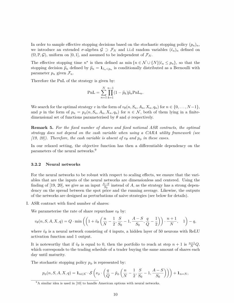
In order to sample effective stopping decisions based on the stochastic stopping policy (pn)n,we introduce an extended σ-algebra G ⊃ FN and i.i.d random variables (εn)n defined on(Ω,P,G), uniform on [0, 1], and assumed to be independent of FN .

The effective stopping time n? is then defined as min n ∈ N ∪ N|εn ≤ pn, so that thestopping decision pn defined by pn = 1εn<pn is conditionally distributed as a Bernoulli withparameter pn given Fn.

Therefore the PnL of the strategy is given by:

PnL =N∑n=1

n−1∏k=1

(1− pk)pnPnLn.

We search for the optimal strategy v in the form of vθ(n, Sn, An, Xn, qn) for n ∈ 0, . . . , N−1,and p in the form of pn = pφ(n, Sn, An, Xn, qn) for n ∈ N , both of them lying in a finite-dimensional set of functions parameterised by θ and φ respectively.

Remark 5. For the fixed number of shares and fixed notional ASR contracts, the optimalstrategy does not depend on the cash variable when using a CARA utility framework (see[19, 20]). Therefore, the cash variable is absent of vθ and pφ in these cases.

In our relaxed setting, the objective function has then a differentiable dependency on theparameters of the neural networks.9

3.2.2 Neural networks

For the neural networks to be robust with respect to scaling effects, we ensure that the vari-ables that are the inputs of the neural networks are dimensionless and centered. Using thefinding of [19, 20], we give as an input A−S

S0instead of A, as the strategy has a strong depen-

dency on the spread between the spot price and the running average. Likewise, the outputsof the networks are designed as perturbations of naive strategies (see below for details).


We parameterise the rate of share repurchase vθ by:

vθ(n, S,A,X, q) = Q ·min((

1 + vθ

(n

N− 1

2 ,S

S0− 1, A− S

S0,q

Q− 1

2

))· n+ 1

N, 1

)− q,

where vθ is a neural network consisting of 4 inputs, a hidden layer of 50 neurons with ReLUactivation function and 1 output.

It is noteworthy that if vθ is equal to 0, then the portfolio to reach at step n + 1 is n+1N Q,

which corresponds to the trading schedule of a trader buying the same amount of shares eachday until maturity.

The stochastic stopping policy pφ is represented by:

pφ(n, S,A,X, q) = 1n∈N · S(νφ ·

(q

Q− pφ

(n

N− 1

2 ,S

S0− 1, A− S

S0

)))+ 1n=N ,

9A similar idea is used in [10] to handle American options with neural networks.

10

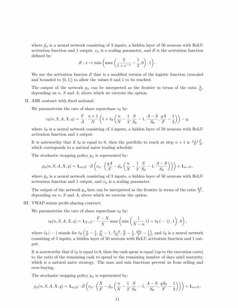
where pφ is a neural network consisting of 3 inputs, a hidden layer of 50 neurons with ReLUactivation function and 1 output, νφ is a scaling parameter, and S is the activation functiondefined by:

S : x 7→ min(

max( 2

1 + e−x− 1

2 , 0), 1).

We use the activation funcion S that is a modified version of the logistic function (rescaledand bounded to [0, 1]) to allow the values 0 and 1 to be reached.

The output of the network pφ can be interpreted as the frontier in terms of the ratio qQ ,

depending on n, S and A, above which we exercise the option.



vθ(n, S,A,X, q) = F

A· n+ 1

N

(1 + vθ

(n

N− 1

2 ,S

S0− 1, A− S

S0,qA

F− 1

2

))− q,

where vθ is a neural network consisting of 4 inputs, a hidden layer of 50 neurons with ReLUactivation function and 1 output.

It is noteworthy that if vθ is equal to 0, then the portfolio to reach at step n + 1 is n+1N

FA ,

which corresponds to a natural naive trading schedule.


pφ(n, S,A,X, q) = 1n∈N · S(νφ ·

(qA

F− pφ

(n

N− 1

2 ,S

S0− 1, A− S

S0

)))+ 1n=N ,

where pφ is a neural network consisting of 3 inputs, a hidden layer of 50 neurons with ReLUactivation function and 1 output, and νφ is a scaling parameter.

The output of the network pφ here can be interpreted as the frontier in terms of the ratio qAF ,




vθ(n, S,A,X, q) = 1X<F ·F −XS

max(

min( 1N − n

(1 + vθ (· · · )) , 1), 0),

where vθ (· · · ) stands for vθ(nN −

12 ,

SS0− 1, A−SS0

, XF −12 ,

qS0F −

12

), and vθ is a neural network

consisting of 5 inputs, a hidden layer of 50 neurons with ReLU activation function and 1 out-put.

It is noteworthy that if vθ is equal to 0, then the cash spent is equal (up to the execution costs)to the ratio of the remaining cash to spend to the remaining number of days until maturity,which is a natural naive strategy. The max and min functions prevent us from selling andover-buying.


pφ(n, S,A,X, q) = 1n∈N · S(νφ ·

(X

F− pφ

(n

N− 1

2 ,S

S0− 1, A− S

S0,qS0F− 1

2

)))+ 1n=N ,

11

where pφ is a neural network consisting of 4 inputs, a hidden layer of 50 neurons with ReLUactivation function and 1 output, and νφ is a scaling parameter.

The output of the network pφ here can be interpreted as the frontier in terms of the ratio XF ,


3.2.3 Objective function approximation

We could use a stochastic gradient descent or a mini-batched gradient descent on the ex-pected CARA utility objective function to approximate an optimal trading and an optimalstopping strategy. However the very fact that the utility is exponential typically causes nu-merical issues. For that reason, we consider the classical Arrow-Pratt (see for instance [33])approximation of the expected CARA utility objective function by a mean-variance objectivefunction:10

−1γ

logE [exp(−γPnL)] ≈ E [PnL]− γ

2V [PnL] .

In our relaxed setting, we have

E [PnL] = E [E [PnL| FN ]]

= E[E[

N∑n=1

n−1∏k=1

(1− pk) pnPnLn∣∣∣∣∣FN

]]

= E[N∑n=1

E[n−1∏k=1

(1− pk) pn∣∣∣∣∣FN

]PnLn

]

= E[N∑n=1

n−1∏k=1

(1− pk) pnPnLn],

since

E[n−1∏k=1

(1− pk) pn∣∣∣∣∣FN

]= E

[n−1∏k=1

(1− 1εk<pk) 1εn<pn

∣∣∣∣∣FN]

=n−1∏k=1

(1− pk) pn,

where we used the fact that (p1, . . . , pn) is FN -measurable, and that ε1, . . . , εn are i.i.d. andindependent of FN .

Similarly,

E[PnL2

]= E

[N∑n=1

n−1∏k=1

(1− pk) pnPnL2n

].

10It is important to note that we could have chosen a mean-variance objective function from the verybeginning. The reason why we started with an exponential utility is to relate our paper to [19, 20].It is also important to recall that the mean-variance approximation of the certainty equivalent associated witha CARA utility function (i) turns out to be exact in the case of Gaussian risks and (ii) corresponds to a firstorder Taylor expansion in the risk aversion parameter (around 0).

12

Subsequently,

−1γ

logE [exp(−γPnL)] ≈ E[N∑n=1

n−1∏k=1

(1− pk)pnPnLn]

−γ2

[E[N∑n=1

n−1∏k=1

(1− pk)pn(PnLn)2]

−(E[N∑n=1

n−1∏k=1

(1− pk)pnPnLn])2 ]

.

Therefore, using a Monte-Carlo approximation with I trajectories of prices (Sin)0≤n≤N,1≤i≤I ,and the resulting stopping policy (pin)1≤n≤N,1≤i≤I and profit and losses (PnLin)1≤n≤N,1≤i≤I ,we can consider the following approximation

−1γ

logE [exp(−γPnL)] ≈ 1I

I∑i=1

N∑n=1

n−1∏k=1

(1− pik)pinPnLin

−γ2

[1I

I∑i=1

N∑n=1

n−1∏k=1

(1− pik)pin(PnLin)2

−(

1I

I∑i=1

N∑n=1

n−1∏k=1

(1− pik)pinPnLin

)2 ].

Given the sampled trajectories (Sin)0≤n≤N,1≤i≤I , the right-hand side of the above equationdepends only on θ and φ. Therefore using automatic differentiation tools we can performgradient descent on this proxy of the objective function.

4 Numerical results

In this section we illustrate the practical use of our method. We consider the reference casedescribed below which corresponds to rounded values for the stock Total SA, deliberatelychosen to be the same as in [20] in order to show that the strategies obtained with our methodare similar to those derived in [20] for an ASR contract with fixed number of shares.

For the same comparison purpose, we train the neural networks with arithmetic Brownianmotion price trajectories Sn+1 = Sn + σ

√δtεn+1, where (εn)n are i.i.d. N (0, 1) random

variables. Contrary to what happens with the method presented in [20], our method can beused with almost any price dynamics or even historical data.11

More precisely, we consider the following market model:

• S0 = 45 €;

• σ = 0.6 €·day−1/2, corresponding to an annual volatility approximately equal to 21%;11Unfortunately, historical time series are often not long enough. A new practice consists in using data

simulated with generative models calibrated to historical data (e.g. generative adversarial networks – see [17]).

13

• T = 63 trading days. The set of possible early exercise dates is N = [22, 62] ∩ N;

• ∀n ∈ 1, . . . , N, Vn = V = 4 000 000 shares· day−1;

• L(ρ) = η|ρ|1+φ with η = 0.1 € ·share−1 · day−1 and φ = 0.75.

4.1 ASR contract with fixed number of shares

For this contract, we consider the following characteristics:

• Q = 20 000 000 shares;

• ` : q 7→ Cq2 for the terminal penalty, where C = 2 · 10−7 € ·share−2;

• ρ = −∞, ρ = +∞, meaning that there is no participation constraints.

Our choice for the risk aversion parameter is γ = 2.5 · 10−7 €−1.

Let us consider three different trajectories for the price in order to exhibit several features ofthe optimal strategy of the bank.

0 10 20 30 40 50 60Time

36

38

40

42

44

46

48

50

52

54

Price

SpotAverage

0 10 20 30 40 50 60Time

0.00

0.25

0.50

0.75

1.00

1.25

1.50

1.75

2.00

Numbe

r of s

hares

1e7

Figure 1: Price trajectory 1 and corresponding strategy for the ASR with fixed number ofshares

0 10 20 30 40 50 60Time

36

38

40

42

44

46

48

50

52

54

Price

SpotAverage

0 10 20 30 40 50 60Time

0.00

0.25

0.50

0.75

1.00

1.25

1.50

1.75

2.00

Numbe

r of s

hares

1e7


14

0 10 20 30 40 50 60Time

36

38

40

42

44

46

48

50

52

54

Price

SpotAverage

0 10 20 30 40 50 60Time

0.00

0.25

0.50

0.75

1.00

1.25

1.50

1.75

2.00

Numbe

r of s

hares

1e7


The first price trajectory exhibits an upward trend. In this case, the optimal strategy ofthe bank consists in buying the shares slowly to minimise execution costs, as illustrated inFigure 1.

The second price trajectory exhibits a downward trend. In that case, the bank has an incentiveto exercise rapidly, even without all the required shares being bought (see Figure 2). Indeed, asthe price stays below its average, the latter is pulled down over time, making it less profitableto postpone the exercise of the option.

The third price trajectory we consider corresponds to the price decreasing and then increasing.As in both preceding examples, we see in Figure 3 that the behaviour of the bank is stronglylinked to the relative position of the price to its running average. At the beginning of thecontract, when the price is below its running average, the bank is acquiring shares at a highpace. Afterwards, when the price goes above its running average, it is not profitable anymorefor the bank to accelerate execution. Instead, the bank is incentivised to delay the exercise ofthe option and it is even selling shares in order to stay close to the strategy qn = n

NQ becausethe risk associated with that strategy is hedged by the payoff of the ASR contract.

Now, as in [20], we study the effects of the parameters on the optimal strategy. More precisely,we focus on the execution cost parameter η and the risk aversion parameter γ.

Let us focus first on execution costs and more precisely on the liquidity parameter η. Weconsider our reference case with 4 values for the parameter η: 0.01, 0.1, 0.2, and 0.5. As wecan see in Figure 4, corresponding to the third price trajectory, the less liquid the stock, thesmoother the optimal strategy to avoid abrupt trading and round trips.

The optimal values of the mean-variance criterion for the different values of the parameter ηare presented in the table below:

η 0.01 0.1 0.2 0.5MeanVarQS0

1.13% 1.05% 0.99% 0.81%

As expected, the more liquid the stock, the more profitable the contract for the bank.

15

0 10 20 30 40 50 60Time

0.00

0.25

0.50

0.75

1.00

1.25

1.50

1.75

2.00

Numbe

r of s

hares

1e7

η=0.01η=0.1η=0.2η=0.5

Figure 4: Effect of execution costs

Let us come now to risk aversion. We consider our reference case with 4 values for theparameter γ: 0, 2.5 · 10−9, 2.5 · 10−7, and 5.0 · 10−7. Figure 5 shows the influence of γ on theoptimal strategy. We see that the more risk averse the bank, the closer to the naive strategy(i.e. qn = n

NQ) its strategy. This is intuitive as the risk associated with this strategy isperfectly hedged by the payoff of the ASR contract. At the other end of the spectrum, whenγ = 0, the corresponding strategy is much more aggressive at the beginning of the contract inorder to be able to benefit from the optionality as soon as possible (because the function ` wehave chosen provides a very strong incentive to have only a few shares to buy at the time ofearly exercise). What prevents the bank from buying instantaneously is just execution costs.An interesting point is also that, when γ = 0, the optimal strategy does not involve any stockselling.12

0 10 20 30 40 50 60Time

0.00

0.25

0.50

0.75

1.00

1.25

1.50

1.75

2.00

Num

ber o

f sha

res

1e7

γ= 0γ= 2.5 ⋅ 10−9

γ= 2.5 ⋅ 10−7

γ= 5.0 ⋅ 10−7

Figure 5: Effect of risk aversion12Since neural networks are just approximations, sometimes we can see some small deviations from the

optimal buy-only strategy in the no risk aversion case.

16

The mean-variance values for the different values of the risk aversion parameter γ are pre-sented in the table below:

γ 0 2.5 · 10−9 2.5 · 10−7 5 · 10−7

MeanVarQS0

1.35% 1.32% 1.05% 0.86%

Unsurprisingly, the more risk averse the bank, the lower the optimal value of the mean-variance criterion.

As our optimisation problem is not convex, the optimisation procedure might lead to a localoptimum. Because of the random initialisation of the neural networks weights and because ofMonte Carlo sampling, the learning process is not always the same. Figure 6 illustrates twovery different learning curves associated with two different instances of the learning procedurewith γ = 5 · 10−7 €−1. We see that the optimisation process for the second instance stalls ina suboptimal state (with a mean-variance score slightly below 0), whereas the first instancemanages to reach a state with a significantly higher score.

0 200 400 600 800 1000Epoch

−200

−150

−100

−50

0

50

100

Crite

rion

Learning curve 1Learning curve 2

Figure 6: Training curve (the unit of the y-axis is MeanVarQS0

expressed in basis points)

0 10 20 30 40 50 60Time

0.00

0.25

0.50

0.75

1.00

1.25

1.50

1.75

2.00

Numbe

r of s

hares

1e7

Figure 7: Locally optimal strategy

17

Interestingly, the suboptimal strategy associated with the second learning instance consists inbuying shares at a constant pace until having the required quantity Q of shares and exercisingimmediately the option, regardless of the price trajectory (see Figure 7). It is not surprisingthat this strategy could be a local optimum as the option payoff provides a perfect hedge forthe execution process.

In order to deter the learner from being caught in the domain of attraction of the type oflocal optimum described above, we can modify the objective function by setting γ to 0 overthe first training epochs in order to remove the incentive to hedge. We refer to this procedureas pretraining.

We illustrate in Figure 8 the learning curve associated with the learning procedure where weperformed pretraining over the first 100 epochs, and we compare it to the two above exampleswithout pretraining. From this graph, we see that pretraining the network helps to avoid thistype of local optimum. Moreover, when pretraining is used, we see in Figure 8 that thelearning curve does not exhibit an intermediate plateau.

0 200 400 600 800 1000Epoch

−200

−150

−100

−50

0

50

100

Crite

rion

With pretrainingWithout pretraining 1Without pretraining 2

Figure 8: Comparison between learning curves with and without pretraining.

Remark 6. It should be mentioned that our pretraining procedure enables to avoid a triviallocal optimum, but does not theoretically ensure the convergence towards a global optimum(this is a common issue in machine learning, especially with neural networks). However,the strategies we obtain are in line with the results of our previous works [19, 20] based onsolving Bellman equations. We believe therefore that our method succeeds in reaching a globaloptimum.

4.2 ASR contract with fixed notional


• F = 900 000 000 €;

• ` : q 7→ Cq2 as terminal penalty, where C = 2 · 10−7 € ·share−2;

• ρ = −∞, ρ = +∞, meaning that there is no participation constraints.

18

We choose the risk aversion parameter γ = 2.5 · 10−7 €−1.

In Figures 9, 10 and 11, we plot the strategies obtained for the fixed notional ASR contract(for the same three price trajectories as above). The targeted number of shares is representedby a solid line (it is not constant due to the stock price change).

0 10 20 30 40 50 60Time

36

38

40

42

44

46

48

50

52

54

Price

SpotAverage

0 10 20 30 40 50 60Time

0.00

0.25

0.50

0.75

1.00

1.25

1.50

1.75

2.00

Numbe

r of s

hares

1e7

Figure 9: Price trajectory 1 and corresponding strategy for the ASR with fixed notional

0 10 20 30 40 50 60Time

36

38

40

42

44

46

48

50

52

54

Price

SpotAverage

0 10 20 30 40 50 60Time

0.0

0.5

1.0

1.5

2.0

Numbe

r of s

hares

1e7


0 10 20 30 40 50 60Time

36

38

40

42

44

46

48

50

52

54

Price

SpotAverage

0 10 20 30 40 50 60Time

0.0

0.5

1.0

1.5

2.0

Numbe

r of s

hares

1e7


19

Now, let us compare the strategies associated with the two types of ASR contract. In Fig-ures 12, 13 and 14, we see that we obtain similar strategies for both types of ASR: acceleratingpurchase when the difference between the average price and the price is positive and deceler-ating purchase or even selling when that difference is negative.

0 10 20 30 40 50 60Time

36

38

40

42

44

46

48

50

52

54

Price

SpotAverage

0 10 20 30 40 50 60Time

0.00

0.25

0.50

0.75

1.00

1.25

1.50

1.75

2.00

Numbe

r of s

hares

1e7

Fixed notionalFixed number of shares

Figure 12: Price trajectory 1 and comparison of the strategies for the two types of ASR

0 10 20 30 40 50 60Time

36

38

40

42

44

46

48

50

52

54

Price

SpotAverage

0 10 20 30 40 50 60Time

0.00

0.25

0.50

0.75

1.00

1.25

1.50

1.75

2.00

Numbe

r of s

hares

1e7



0 10 20 30 40 50 60Time

36

38

40

42

44

46

48

50

52

54

Price

SpotAverage

0 10 20 30 40 50 60Time

0.00

0.25

0.50

0.75

1.00

1.25

1.50

1.75

2.00

Numbe

r of s

hares

1e7



20

4.3 VWAP-minus profit-sharing contract


• F = 900 000 000 €;

• α = 25%;

• κ = 0.5%;

• ` : x 7→ Cx2 as terminal penalty, where C = 2 · 10−9 €−1;

• ρ = 0, ρ = +∞, reflecting the prohibition to sell.

To manage the contract, we consider the modified payoff described in Remark 2 and inSection 3.1.2 with β = 5%: the bank does not only get part of the profit but also part of theloss.

We choose γ = 10−6 €−1 so that αγ = 2.5 · 10−7.

0 10 20 30 40 50 60Time

36

38

40

42

44

46

48

50

52

54

Price

SpotAverage

0 10 20 30 40 50 60Time

0.0

0.2

0.4

0.6

0.8

Cash sp

ent

1e9

Figure 15: Price trajectory 1 and corresponding strategy for the VWAP-minus profit-sharingcontract

0 10 20 30 40 50 60Time

36

38

40

42

44

46

48

50

52

54

Price

SpotAverage

0 10 20 30 40 50 60Time

0.0

0.2

0.4

0.6

0.8

Cash sp

ent

1e9


21

0 10 20 30 40 50 60Time

36

38

40

42

44

46

48

50

52

54

Price

SpotAverage

0 10 20 30 40 50 60Time

0.0

0.2

0.4

0.6

0.8

Cash sp

ent

1e9


The strategies obtained with our neural network algorithm for this type of contract are plottedin Figures 15, 16 and 17.13 Here we represent our strategy in terms of the cash spent inrepurchasing because cash is the crucial variable for this contract.

We see that the strategy consists in accelerating the purchase process when the price goesbelow its average and decelerating it when the price increases above its average. In the caseof this contract, there is no round trip as selling is prohibited. This explains in particular theshape of the execution strategy in the case of the third price trajectory.

It is interesting to notice (see Figures 18, 19 and 20) that this strategy is similar to thatof an ASR contract with fixed number of shares (with the same trading constraints) whenone compares the proportion of the cash spent in the case of the former contract with theproportion of shares bought in the case of latter contract.

0 10 20 30 40 50 60Time

36

38

40

42

44

46

48

50

52

54

Price

SpotAverage

0 10 20 30 40 50 60Time

0.0

0.2

0.4

0.6

0.8

1.0

Prop

ortio

n

Profit sharingFixed number of shares (selling prohibited)Fixed number of shares

Figure 18: Price trajectory 1 and comparison of the strategies13It must be mentioned that, in the case of this type of contract, we used the value C = 0.01

Ffor the final

penalty function during the pretraining phase.

22

0 10 20 30 40 50 60Time

36

38

40

42

44

46

48

50

52

54

Price

SpotAverage

0 10 20 30 40 50 60Time

0.0

0.2

0.4

0.6

0.8

1.0

Prop

ortio

n


Figure 19: Price trajectory 2 and comparison of the strategies

0 10 20 30 40 50 60Time

36

38

40

42

44

46

48

50

52

54

Price

SpotAverage

0 10 20 30 40 50 60Time

0.0

0.2

0.4

0.6

0.8

1.0

Prop

ortio

n


Figure 20: Price trajectory 3 and comparison of the strategies

Conclusion

In this paper, we propose a machine learning approach involving recurrent neural networksto find the optimal strategy associated with different types of VWAP-minus program: ASRswith fixed number of shares, ASRs with fixed notional, and profit-sharing contracts. Theresults we obtain are in line with both intuition and previous studies. The interest of ourmethod lies in the fact that almost any price dynamics can be considered and that new typesof contract can be handled. In particular, we manage to handle contracts for which classicalmethods usually fail because of (i) high dimensionality and (ii) the very complexity of somecontracts that cannot be written as payoffs.

23

Appendix

In this appendix, we propose a brief introduction to neural networks and their use for ap-proximating functions. We also briefly expose their interest for solving optimisation problems.Finally, we describe the networks used in this paper with a focus on their recurrent struc-ture.

A bit of history

In the 1950s, decisive results were obtained regarding representations of real continuous func-tions of several variables through addition and composition of continuous functions dependingon a smaller number of variables. First, Kolmogorov obtained in [26] a representation withfunctions of three variables. Then, Arnold, his 19-year-old student at that time, obtained arepresentation with functions of two variables (see [5]), thus providing an answer to the con-tinuous (as opposed to algebraic) version of Hilbert’s thirteenth problem. Finally, Kolmogorovderived in [27] his celebrated superposition theorem stating the existence of a representationby superpositions of continuous functions of one variable:

Theorem 1 (Kolmogorov’s superposition theorem). Let n ≥ 2 be an integer. There existreal continuous functions (φp,q)1≤p≤n,1≤q≤2n+1 defined on [0, 1] such that for any real contin-uous function f defined on [0, 1]n, there exist real continuous functions (χq)1≤q≤2n+1 definedon [0, 1] such that

∀(x1, . . . , xn) ∈ [0, 1]n, f(x1, . . . , xn) =2n+1∑q=1

χq

n∑p=1

φp,q(xp)

.This result has then been improved in many ways, from reducing the number of necessary func-tions, to imposing monotonicity, Lipschitz, or Hölder conditions on the functions. However,despite constructive proofs of superposition theorems, real computation of representationsremains almost always impossible because constructions always involve limits, hence infiniteloops. Furthermore, the functions involved are often unreasonably complicated because thegoal is to obtain a representation rather than an approximation.

Function approximation with neural networks

In fact, an important strand of research has been dedicated to obtain approximate represen-tations with simple functions of a single variable. In particular, feedforward neural networksare often regarded as good candidates for approximating nonlinear functions.

A feedforward neural network is a function of the form ΨL (for L ≥ 1 an integer) where(Ψl)0≤l≤L are defined recursively14 by Ψ0 : x ∈ Rd0 7→ x and

Ψl : x ∈ Rdl−1 7→ gl(AlΨl−1(x) + bl), ∀l ∈ 1, . . . , L,14Layer 0 is called the input layer while layer L is called the output layer.

24

where for each layer l ∈ 1, . . . , L, gl : (x1, . . . , xdl) ∈ Rdl 7→ (hl(x1), . . . , hl(xdl)) ∈ Rdlapplies elementwise either the identity function or a nonlinear function called activation func-tion (in the latter case hl is typically a sigmoid function, the hyperbolic tangent function,a softmax function, or the rectified linear unit (ReLU) function – i.e. x ∈ R 7→ x1x≥0),Al ∈ Rdl×dl−1 is a matrix of weights, and bl ∈ Rdl a vector of weights also called bias. Afeedforward neural network is often denoted by Ψθ where θ = (Al, bl)1≤l≤L stacks all theparameters.

In addition to the link with neurons and the functioning of the animal/human brain (on whichwe shall remain silent throughout this short appendix), the main interest of feedforward neuralnetworks lies in universal approximation theorems such as the one proved by Hornik in [22].In a nutshell, these theorems state, under various – and usually mild – hypotheses, that anyreal function of several variables (here d0 variables) can be approximated by a feedforwardneural network of the above form, provided that there are sufficiently many neurons (i.e. djfor j ∈ 1, . . . , J large enough). More precisely, Hornik [22] proved the following universalapproximation theorem for continuous functions:15

Theorem 2 (Hornik’s universal approximation theorem). Let K be a compact set of Rd0.Let h be a real-valued continuous, bounded, and nonconstant function defined on R. Thenx ∈ K 7→

d1∑j=1

A21,jh

d0∑k=1

A1j,kxk + b1

k

∣∣∣∣∣∣ d1 ∈ N∗, A1 ∈ Rd1×d0 , b1 ∈ Rd1 , A2 ∈ R1×d1

is dense in the set C(K) of real continuous functions defined on K.

Most of early universal approximation theorems state that one hidden layer with an activationfunction and a second output layer is sufficient to obtain a good approximation. However, andthis is why deep learning is so important, it is often more efficient to approximate a functionwith several layers consisting of a few neurons than with one layer with a lot of neurons.

Remark 7. It is noteworthy that, in this paper, neural networks with one hidden layer anda few dozens of neurons were sufficient to obtain satisfactory results.

Optimisation with neural networks

Feedforward neural networks allow to approximate a large class of functions but so do otherfamilies of functions. The reasons why they are often favored have to do with (i) the def-inition (or characterisation) of the functions to be approximated in machine learning, (ii)the possibility to compute Ψθ(x) and its gradient with respect to θ in an efficient way usingforward and backward propagation respectively (see for instance [16] for an introduction),and (iii) the fact that approximations with feedforward neural networks of functions definedon a high-dimensional space are often parsimonious, hence the advantage of neural networksover other families of functions in front of the curse of dimensionality.

15Hornik also proved a Lp version of the universal approximation theorem. Many other versions of thistheorem exist, for instance to handle ReLU activation functions which are unbounded.

25

In machine learning indeed, be it for supervised, unsupervised, or reinforcement learning, theproblem often boils down to approximating a function defined as the solution to an optimi-sation problem. Therefore, the ability to efficiently differentiate the function with respect toits parameters is essential to use all the classical techniques of gradient descent.16

Recurrent network structure

In this paper we use neural networks to approximate two functions: the optimal trading strat-egy of the trader and its optimal stopping decision in the form of a probability to exercise theoption. These functions depend, in general, on the time to maturity, the cash spent since in-ception, the current price of the stock, its running average since the beginning of the contract,and the number of shares already acquired. The problem is discretised in time and decisionsmade at any time step influence the state at all future time steps including the final one. Inparticular, the learning procedure to optimise the mean-variance objective function requiresto take into account all subsequent effects when computing the derivatives with respect to theweights of the neural networks involved in the decisions taken at a time period n < N − 1.

Formally speaking, the trading decision made at a period n < N−1, i.e. vθ(n, Sn, An, Xn, qn)where θ stands as always for the parameters of the neural network, allows to compute the nextvalue of the inventory process, i.e. qn+1 = qn + vθ(n, Sn, An, Xn, qn)δt, which enters as aninput in the network to compute the next trading decision vθ(n+ 1, Sn+1, An+1, Xn+1, qn+1),and so on (in the case of the profit-sharing contract the same problem occurs with the cashvariable). As a consequence, the networks involved in our approach are recurrent. This doesnot however raise any technical difficulty for computing gradients because we use automaticdifferentiation.17

References

[1] Ali Akyol, Jin S. Kim, and Chander Shekhar. The causes and consequences of acceleratedstock repurchases. International Review of Finance, 14(3):319–343, 2014.

[2] Franklin Allen and Roni Michaely. Payout policy. In Handbook of the Economics ofFinance, volume 1, pages 337–429. Elsevier, 2003.

[3] Robert Almgren and Neil Chriss. Value under liquidation. Risk, 12(12):61–63, 1999.

[4] Robert Almgren and Neil Chriss. Optimal execution of portfolio transactions. Journalof Risk, 3:5–40, 2001.

[5] Vladimir I Arnold. On functions of three variables. collected works: Representations offunctions. Celestial Mechanics and KAM Theory, 1965:5–8, 1957.

16The examples of this paper have been computed using the open-source package TensorFlow, distributedby Google.

17Recurrent structures are sometimes prone to vanishing gradient problems. However, we never noticed anysuch problem while using our methods.

26

[6] Ladshiya Atisoothanan, Balasingham Balachandran, Huu Nhan Duong, and MichaelTheobald. Informed trading in option markets around accelerated share repurchase an-nouncements. In 27th Australasian Finance and Banking Conference, 2014.

[7] Achref Bachouch, Côme Huré, Nicolas Langrené, and Huyen Pham. Deep neural net-works algorithms for stochastic control problems on finite horizon, part 2: numericalapplications. 2018.

[8] Leonce Bargeron, Manoj Kulchania, and Shawn Thomas. Accelerated share repurchases.Journal of Financial Economics, 101(1):69–89, 2011.

[9] Christian Beck, Sebastian Becker, Philipp Grohs, Nor Jaafari, and Arnulf Jentzen. Solv-ing stochastic differential equations and kolmogorov equations by means of deep learning.2018.

[10] Sebastian Becker, Patrick Cheridito, and Arnulf Jentzen. Deep optimal stopping. Journalof Machine Learning Research, 20(74):1–25, 2019.

[11] Hans Buehler, Lukas Gonon, Josef Teichmann, and Ben Wood. Deep hedging. Quanti-tative Finance, pages 1–21, 2019.

[12] Thomas J. Chemmanur, Yingmei Cheng, and Tianming Zhang. Why do firms undertakeaccelerated share repurchase programs? 2010.

[13] Kai Chen. News management and earnings management around accelerated share re-purchases. 2017.

[14] Yung-Chin Chiu and Woan-Lih Liang. Do firms manipulate earnings before acceleratedshare repurchases? International Review of Economics & Finance, 37:86–95, 2015.

[15] Joan Farre-Mensa, Roni Michaely, and Martin Schmalz. Payout policy. Annual Reviewof Financial Economics, 6(1):75–134, 2014.

[16] Ian Goodfellow, Yoshua Bengio, and Aaron Courville. Deep learning. MIT press, 2016.

[17] Ian Goodfellow, Jean Pouget-Abadie, Mehdi Mirza, Bing Xu, DavidWarde-Farley, SherjilOzair, Aaron Courville, and Yoshua Bengio. Generative adversarial nets. In Advancesin neural information processing systems, pages 2672–2680, 2014.

[18] Olivier Guéant. The Financial Mathematics of Market Liquidity: From optimal executionto market making, volume 33. CRC Press, 2016.

[19] Olivier Guéant. Optimal execution of ASR contracts with fixed notional. Journal ofRisk, 19(5):77–99, 2017.

[20] Olivier Guéant, Jiang Pu, and Guillaume Royer. Accelerated share repurchase: pric-ing and execution strategy. International Journal of Theoretical and Applied Finance,18(03):1550019, 2015.

[21] Jiequn Han, Arnulf Jentzen, and E Weinan. Solving high-dimensional partial differen-tial equations using deep learning. Proceedings of the National Academy of Sciences,115(34):8505–8510, 2018.

[22] Kurt Hornik. Approximation capabilities of multilayer feedforward networks. Neuralnetworks, 4(2):251–257, 1991.

27

[23] Côme Huré, Huyên Pham, Achref Bachouch, and Nicolas Langrené. Deep neural networksalgorithms for stochastic control problems on finite horizon, part i: convergence analysis.2018.

[24] Sebastian Jaimungal, Damir Kinzebulatov, and Dmitri Rubisov. Optimal acceleratedshare repurchases. Applied Mathematical Finance, 24(3):216–245, 2017.

[25] Tao-Hsien Dolly King and Charles E. Teague. Accelerated share repurchases: Valuecreation or extraction. 2017.

[26] Andreı Kolmogorov. The representation of continuous functions of several variables bysuperpositions of continuous functions of a smaller number of variables.

[27] Andreı Kolmogorov. The representation of continuous functions of several variables bysuperpositions of continuous functions of one variable and addition.

[28] Manoj Kulchania. Market micrsotructure changes around accelerated share repurchaseannouncements. Journal of Financial Research, 36(1):91–114, 2013.

[29] Ahmet C. Kurt. Managing eps and signaling undervaluation as a motivation for repur-chases: The case of accelerated share repurchases. Review of Accounting and Finance,17(4):453–481, 2018.

[30] Carol A Marquardt, Christine Tan, and Susan M Young. Accelerated share repurchases,bonus compensation, and CEO horizons. In 2012 Financial Markets & Corporate Gov-ernance Conference, 2011.

[31] Allen Michel, Jacob Oded, and Israel Shaked. Not all buybacks are created equal: Thecase of accelerated stock repurchases. Financial Analysts Journal, 66(6):55–72, 2010.

[32] Merton Miller and Franco Modigliani. Dividend policy, growth, and the valuation ofshares. 1961.

[33] John W Pratt. Risk aversion in the small and in the large. In Uncertainty in Economics,pages 59–79. Elsevier, 1978.

[34] E Weinan, Jiequn Han, and Arnulf Jentzen. Deep learning-based numerical methodsfor high-dimensional parabolic partial differential equations and backward stochasticdifferential equations. Communications in Mathematics and Statistics, 5(4):349–380,2017.

[35] J Fred Weston and Juan A Siu. Changing motives for share repurchases. 2003.

[36] Ken C. Yook and Partha Gangopadhyay. The wealth effects of accelerated stock repur-chases. Managerial Finance, 40(5):434–453, 2014.

28

accelerated share repurchase and other buyback programs

Documents