Academic Salaries and

Public Evaluation of University Research:

Evidence from the UK Research Excellence Framework∗

Gianni De Fraja† Giovanni Facchini‡ John Gathergood§

April 11, 2019

Abstract

We study the effects of public evaluation of university research on the pay structures of academicdepartments. A simple equilibrium model of university pay determination shows how thepay-performance relationship can be explained by the incentives inherent in the researchevaluation process. We then analyse the pay-performance relationship using data on the salary ofall UK university full professors, matched to the performance of their departments from the 2014UK government evaluation of research, the Research Excellence Framework (REF). A crosssectional empirical analysis shows that both average pay level and pay inequality in a departmentare positively related to performance. It also shows that the pay-performance relationship isdriven by a feature of the research evaluation that allows academics to transfer the affiliation ofpublished research across universities. To assess the effect of the REF on pay structure, we takeadvantage of the time dimension of our data and of inherent uncertainty in the evaluation of theperformance of academic departments generated by the rules of the exercise. Our results indicatethat higher achieving departments benefit from increased subsequent hiring and higherprofessorial salaries with the salary benefits of REF performance concentrated among the highestpaid professors.

Keywords: Research evaluation, Research funding, Research Excellence Framework.JEL Codes: D47, H42, I28, L30.

∗We are grateful to Andrea Ichino for his editorial guidance, Benjamin Born and Martin Halla of the Economic PolicyPanel for their extensive and helpful comments on earlier versions of our paper, Cecilia Testa, Jacques Maraisse, JosepAmer Mestre, Paula Stephan, Todd Zangler, three anonymous referees of this journal and the audiences at the 2017 RESConference in Bristol, at the 2017 BRICK Workshop on the Economics of Science (Turin), at the 2017 Barcelona GSE Forum,the 2017 AISUK conference, and at the 68th Economic Policy Panel meeting at the Oesterreichische Nationalbank in October2018 for helpful comments.

†University of Nottingham, School of Economics, Università di Roma “Tor Vergata”, and C.E.P.R. Email:gianni.defraja@nottingham.ac.uk.

‡University of Nottingham, School of Economics, Università degli Studi di Milano, C.E.P.R. and GEP. Email:giovanni.facchini@nottingham.ac.uk.

§University of Nottingham, School of Economics and Network for Integrated Behavioural Science. Email:john.gathergood@nottingham.ac.uk.

1 IntroductionMany countries, particularly in Europe, have in recent years introduced public evaluation of thescientific research carried out by universities. The outcome of these evaluations affects directly theallocation of public funding to the university sector and is an important input to produce rankingsused by students, industry, the media, and other users to measure university quality. In this paperwe study the effects of a national research evaluation of academic departments on departmentalwage structure using a rich dataset covering all UK universities. Two features of the UK setting makeit ideally suited to study this question. First, the UK has a systematic and comprehensive assessmentof research provided by the Research Excellence Framework (REF). This determines the government“block” research funding, a significant source of research income for UK institutions. The importanceof REF performance is also leveraged by its contribution to the ranking published in severaluniversity league tables. As a result, it also affects indirectly other sources of research income,post-graduate student recruitment,1 and prestige. Second, unlike many other European countries,the size of academic departments and full professors’ compensation are not subject to nationalregulation, other than an agreed minimum salary. Hence universities are free to determineprofessorial hirings and set professorial pay. Indeed, our data exhibits large observed salarydifferences, with the highest paid professors in some of the elite institutions earning as much asseven times the national minimum. A fundamental question is then how performance in the REFtranslates to wage structures at the department level.

Our analysis draws upon a dataset comprising details of salaries paid to full professors at all UKdepartments between 2013 and 2016 and the performance of their department in the REF carried outin 2014. Together, these data allow us to evaluate the association between the department’s paystructure and its performance in the REF and the effects of departmental performance on subsequentoutcomes. The university sector in the UK is an example of a quasi-market, where individualinstitutions compete, often fiercely, according to rules designed by the government to mimic theincentive system operating in the private markets. In the latter, the literature (e.g. Nickell andWadhwani 1990, Nickell et al. 1994, Hildreth and Oswald 1997, Abowd et al. 1999, and Lazear 2000)has long firmly established a positive correlation between firm performance and average pay. Someevidence suggests also that firms with higher within-firm pay inequality might improve performance(Grund and Westergaard-Nielsen 2008, Edmans and Gabaix 2016, Mueller et al. 2017). Our firstcontribution is to analyse whether this also holds true for universities. A subject of amused or heateddiscussions among academics, there is surprisingly little systematic evidence on this importantquestion. Stephan (2012) finds that, in the three decades prior to 2006, salary inequality by rank morethan doubled for every rank in US academia within four broad areas, namely engineering,maths/computer science, physical sciences, and life sciences. Otherwise the literature is limited, andhas focused on broad national differences in university pay (Altbach et al. 2012) or the internal labormarkets of universities (Oyer 2007, Haeck and Verboven 2012) rather than variation amonginstitutions within a country.

1This can be an important source of funding for some departments; income from undergraduate students, on the otherhand, is unlikely to be affected by a good REF performance. This is so both because fees are capped, and because studentschoose on the basis of word of mouth information from their teachers, or from newspaper rankings which give a negligibleweight to research.

1

To frame our analysis, we present a theoretical model of university pay determination whereuniversities face a national competitive evaluation of their research, and aim at maximising anaggregate measure of research success. This in turn determines the research funding they will receivefrom the government. Research is produced using elastically supplied capital and different kinds oflabour, to capture the diverse attributes of the academics employed. Among the various models thatcan be built to capture the structure of the university sector, and the internal organisations ofindividual universities, our model allows us to highlight the key role played by the internal wagestructure and predicts a positive correlation between the research performance of a department, theaverage salary of its staff, and inequality in departmental pay.

Our empirical analysis consists of two conceptually distinct parts. In line with the theoreticalmodel, in Section 4 we uncover a positive cross-sectional relationship between professorial pay inUK universities and their 2014 REF performance. This is best interpreted as capturing thesteady-state, static equilibrium of the theoretical model. This finding is very robust: it holds when wecontrol for a range of departmental characteristics and for academic discipline and university typefixed effects. It also holds across the whole range of academic disciplines. Interestingly, we find thatthe pay-performance relationship is weaker, though still statistically significant, in the mostwell-known research intensive universities, and stronger among those established more recently. Wealso find a positive relationship between professorial pay inequality within a department and REFperformance at the department level. Unlike for the mean salary, this finding is strongest in the mostprestigious universities, and is statistically significant for disciplines in the sciences and engineering,but not in medicine and biology, the social sciences, the arts and humanities.

In Sections 5 and 6 we study instead the effects of the assessment on the subsequent evolution ofa department’s composition and wage structure. To do so, we exploit the existence of two distinctmeasures of performance. First, the funding score received by a department determines the financialtransfer made by the government funding agency to the university. Second, the grade point averagescore (GPA) is the headline perceived quality measure (reputation) used to compare departmentsacross institutions and disciplines. These two scores are calculated differently – see Box 3 for moredetails – and their correlation, while positive, is far from perfect. As a result, it might well happenthat two departments with the same reputation, measured by the GPA, receive different fundingallocations; and analogously two departments with the same funding score could be rankeddifferently according to GPA. Importantly, these difference are unlikely to be perfectly anticipated bythe institutions and their highly unpredictable nature likens them to a random allocation ofadditional funding to some departments, in preference to others, observationally very similar.Difference-in-differences estimates on a matched sample of departments therefore allows us toestimate the independent effects of funding conditional on research quality (and vice-versa) onsubsequent developments in the composition and pay structure of the department

Our findings show that departments which obtain a stronger REF result see faster subsequentgrowth in wages and professorial headcount compared with less performing, but otherwise similardepartments. Importantly, this effect is statistically significant only when performance is measuredby GPA, but not when it is measured through research funding allocations. One plausibleinterpretation of these results is that the REF affects departments primarily through establishing an

2

objective measure of reputation (GPA score) and not as much through funding. Thus the vauntedgovernment policy of rewarding excellence, by steering funding heavily where “world leading”research is carried out is partially undone by the universities’ central administrations, which appearto allocate more senior posts according to the simpler GPA measure. In other words, the researchevaluation exercise seems to create a measure of research quality, and departments which performstrongly in terms of research quality are rewarded with higher wages and new senior posts.

Both the theoretical model and the empirical analysis link average pay and research performanceat the department level. As a result, the focus of our study differs from that in the relatively moreestablished literature linking individual’s compensation and their research productivity, where greatattention has been dedicated to the challenging task of measuring an academic’s output. The earlywork by Diamond (1986) uses citations as an indicator of a researcher’s impact, and finds that themarginal effect of an additional citation on individual income is positive. Other contributionsdistinguish between the number of citations, used as a proxy for “quality”, and the measure of“quantity” given by the number of papers published. Most analyses study a small sample ofdepartments (e.g. Hamermesh et al. 1982, Moore et al. 1998 and Bratsberg et al. 2010). In a recentpaper, Hamermesh and Pfann (2012) consider instead the members of a larger group of 43 economicsdepartment at public institutions in the United States, and find a positive association between outputand salaries. This holds both when output is measured by quality, proxied by citations, or byquantity, the number of papers. As far as we know, Sgroi and Oswald (2013) is the only paper whichprovides a solid theoretical foundation to the balance between quality and quantity. The paucity ofinformation on individual pay has constrained the analysis of the previous incarnations of the REF.2

A small recent strand of this literature studies the determinants of individuals’ research output incontinental Europe: among these, Bosquet and Combes (2017), Zinovyeva and Bagues (2010, 2015) andChecchi et al. (2014) in France, Spain, and Italy, respectively. The first of these studies shows that thecharacteristics of colleagues matter for research, while the last two focus on the link between researchperformance and the chances of promotion. In a recent contribution Kwiek (2017), on the other hand,shows how in continental Europe salary increases are associated with increases in administrative andmanagerial duties.

The rest of the paper proceeds as follows. To frame our analysis, we present in Section 2 a simpletheoretical model of resource allocation within universities that we use to interpret our empiricalresults. The main features of the REF and the data used in the analysis are described in Section 3.Our empirical results are presented in Sections 4, 5 and 6. Section 7 concludes. Additional results andmore information on the UK university sector are available in the Appendix.

2Early comprehensive studies (e.g. Johnes et al. 1993, Taylor 1995, Sharp and Coleman 2005) have emphasised the roleplayed by systematic biases in the panels’ quality assessment, based on characteristics of the institutions: new universitiesvs. more established ones, institutions based in England vs. those based in other parts of the country, units of assessment thathad a panel member vs. those which did not, and so on. Controlling for the quality of the submission in the 1996 and 2001assessments of economics and econometrics departments, Clerides et al. (2011) do not find systematic evidence of biases infavour of specific institutions. The exception is membership in the assessment panel, which has a positive and significantimpact on the ranking of the department in the 1996 exercise. This is in line, as well as with this paper, with Butler andMcAllister’s (2009) study of the evaluation of the political science panel in the 2001 exercise. The important role played bythe panel composition on the evaluation process of academics has been emphasised also by Zinovyeva and Bagues (2015)for the case of Spain.

3

2 A Model of Research Evaluation and University CompetitionBoxes 1 and 2 present a simple theoretical model which illustrates how the incentives created by theresearch evaluation exercise may shape the pay structure within a university’s academic departments.While other models of the university sector are of course possible, we build one that allows us tofocus on the effects of the competition induced by the REF, and so we concentrate on the productionof research, abstracting, in particular, from explicitly including teaching. Any constraint imposed byteaching, such as the requirement to recruit a given number of students, is implicitly captured in theproduction function or in the budget constraint.

In our simple model, research output is generated by different units within a university, thedepartments. All units employ capital and two types of academics (good and excellent professors),and they may differ in their “technology”, captured by the extent of the complementarity betweenthe three inputs, capital and the two types of labour. Universities allocate their budget acrossdifferent departments in order to maximise a weighted average of the research outputs of all theirdepartments3 and receive transfers from the government which depend on the research performanceof each unit. Capital is elastically supplied, and we capture the scarcity of academic labour with asimple reduced form supply function, inelastic for both types of labour, but, naturally, more so formore skilled academics. With this model, we determine the wage structure of each department andthe allocation of funds across departments in each state financed university.

We begin, in Box 1, by studying the problem faced by a department which needs to allocate thebudget it receives from the central administration of the university. Lemma 1 in Box 1 indicates that,in the long run, the industry equilibrium is such that the amount of both capital and labouremployed by a department increase with the budget allocated to it, whereas the amount of labour(capital) employed declines (increases) with the importance of capital in the production process. Thislatter parameter influences research output in unexpected ways: small departments become smallerstill as capital intensity increases, whereas large ones instead increase further in size. This tallies withthe anecdotal observation that capital intensive departments tend to be large.4

Expression (9) in Lemma 2 is standard for models where labour supply is inelastic. Expression(10) shows that the mean salary and the dispersion of salaries within a department are collinear, andProposition 1 shows that they both increase with the budget allocated to the department, and with theimportance of labour in the production process of research. Intuitively, the mean increases becauseof the realistic assumption that the labour supply is not perfectly elastic. As labour becomes morevaluable, for example because the university allocates more funding to the department, or becausecapital becomes less important, the department will want to hire more academics of both types, andsupply being inelastic, will need to pay more for it.

3While a large body of literature emphasises the role played by conflicts of interest within large institutions (Milgromand Roberts, 1992), in the case of universities it is plausible to assume that individual academics and the heads of bothuniversities and departments all share the same goal with regards to research, namely the maximisation of its quality.

4This follows from the fact that the sign of the derivative of output with respect to the parameter βi is the same as thesign of ln 2βi Bi

cir : therefore it is negative when the budget is low, but it becomes positive for a large enough budget.

4

BOX 1 The department optimisation problemWe model the higher education sector as a quasi-market comprising K universities, indexed byk = 1, . . . , K. They aim to maximise an aggregate measure of their research output in the nacademic disciplines, indexed by i = 1, . . . , n.Research is produced using three inputs: capital and two types of labour, for example, goodprofessors and superstar academics. Let w` be the salary of an academic of type ` and assumethat the supply of this type of professors is given by a

L` = µ`w`, ` = 1, 2, (1)

where L` is the amount of labour of type `, with ` = 1, 2. The parameter µ` in the supplyfunction of the two types of labour captures plausibly different job market opportunities forthe two types of academics, which depend on their research potential. The research outputb

of university k in discipline i, k = 1, . . . , K, i = 1, . . . , n, is denoted by ρk,i, and obeys aCobb-Douglas technology, a simplified special case of the functions typically used in empiricalanalyses of universities’ production function (for example Thanassoulis et al. (2011)):

ρk,i = θkLα11 Lα2

2 Sβi , (2)

where S is the stock of capital, given by labs, equipment, technical personnel, and so on: thiscan be purchased in a competitive market at a price r.The parameters θk and βi correspond to fixed effects in our empirical specification. Theycharacterise respectively the overall research productivity of an institution, due for example todifferent research environments and international connections,c and the importance of capitalin a given discipline, which depends on factors such as laboratory costs and the like.If a given department i receives a fixed budget Bi from university k central administration, itsbudget constraint is given by:

rS + w1L1 + w2L2 = Bi. (3)

Thus department i in institution k chooses S, L1 and L2 to maximise (2) subject to (1) and (3). Tolighten notation, let

aWe therefore ignore any oligopsonistic interaction among institutions: taking them into account would changethe absolute levels of academic employment and salaries, but would not alter their relative values across institutionsand disciplines, which is the focus of our paper.

bWe do not specify how research output is measured. It could be one of the REF measures considered below,(19) or (20), but the model could be applied to a world without REF, and research output is the less mechanicallydefined prestige and reputation that is fed and maintained by prizes, accolades, publications, policy influence, andany distinction that enhances academic esteem.

cWe take θk to be exogenously given: it may depend on reputation, history or location, and in particular, it is notaffected by changes in the quality of other departments. Thus our analysis is based on the idea that the correlationbetween the quality of the various departments in a given university is not a necessary consequence of technologicalspillovers, but may be caused by an unobserved factor, common to all departments. A similar set-up emerges if θkis interpreted as a measure of the cost of doing research, and if the plausible assumption is made that academicsare willing to trade-off a university’s prestige and overall research environment for a lower salary (see De Fraja andValbonesi (2012), or De Fraja (2016)). If this is the case a prestigious university would find it easier to hire and retainhigh quality academics and for this reason enjoy a higher productivity.

5

Ai = αα12

1 µα12

1 αα22

2 µα22

2

(2βi

r

)βi

, (4)

ci = α1 + α2 + 2βi. (5)

We can now establish the following:

Lemma 1. The solution of the maximisation problem of department i in institution k satisfies:

L` =

√α`µ`

ciBi, ` = 1, 2, (6)

S =2βi

ci

Bi

r, (7)

and the research output is given by

ρ∗k,i (Bi) = θk Ai

(Bi

ci

) ci2

. (8)

The wage structure of the department is instead characterized in the following:

Lemma 2. At the solution of department i’s maximisation problem the salaries for the two types ofacademics are given by:

w` =

√α`Bi

ciµ`, ` = 1, 2. (9)

Therefore the mean salary and its standard deviation are given by

w̄ =α1 + α2√

α1µ1 +√

α2µ2

√Bi

ci, σw =

∣∣∣√ α1µ1−√

α2µ2

∣∣∣√

α1µ1 +√

α2µ24√

α1µ1α2µ2

√Bi

ci, (10)

and the Gini coefficient of the department members’ pay by:

Gi =

√α1α2

(√µ1α2 −

√µ2α1

)(α1 + α2)

(√µ1α1 +

√µ2α2

) . (11)

The proof of this and the other results can be found in the Appendix. The following is animmediate consequence of the previous result.

Proposition 1. The derivatives of the mean salary and of the standard deviation of salary in department

i in institution k are proportional to the derivative of√

Bici

. This is −c−32

i B12i < 0, when differentiating

with respect to βi, and 12 c−

12

i B−12

i > 0 when differentiating with respect to Bi.

6

The increase in the standard deviation requires the additional hypothesis that the ratio αlµl

is

different for the two types of labour, so that the∣∣∣√ α1

µ1−√

α2µ2

∣∣∣ in (10) is non-zero.5 As long as the twotypes of labor have different efficiency adjusted costs, as the size of the department increases, so doesthe wedge between the total compensation of the two groups of workers, and hence the measuredstandard deviation of departmental salaries. While the exact values of individual wages, aggregatewages and of the Gini coefficient in (9)-(11) does depend on the assumption of a Cobb-Douglastechnology, the informal discussion in this paragraph suggests that the relationships highlighted inProposition 1 will hold more generally, when at least some workers are paid above their marginalproductivity.6

Given that, ceteris paribus, a department’s research output increases with its budget, the modelpredicts a positive association in the steady-state equilibrium between average salary and researchoutput and between inequality in salary and research output, which is consistent with the mainfindings of our empirical analysis. Conversely, the mean and the standard deviation of thedepartment salaries varies in the opposite direction to capital intensity. The intuition for this effect isthe same as for size: an increase in β reduces the importance of labour in production, and so, for agiven budget, fewer workers will be employed.7

Corollary 1 in Box 2 implies that, in the steady state, universities with a higher ability to doresearch, measured by θk in the model, will be able to devote more resources to all their departments,which will also produce higher output. In other words, in equilibrium, research output and the paystructure of each department in every institution are simultaneously determined by the commontechnology, captured by the parameters α1, α2, and βi, with a ranking of institutions determinedinstead by the unobservable idiosyncratic parameter θk. This ranking suggests that some institutionswill tend to perform better in all disciplines, and pay their professors more.8 As a result, our modelcan explain the empirical pattern that some groups of universities tend to perform better in theresearch evaluation across (nearly) all disciplines – for example the Russell Group in the UK context.

5Note that it is theoretically conceivable that the lower productivity workers are paid more. For this to happen, however,their supply must be sufficiently more inelastic than that of higher productivity workers to compensate for their lowerproductivity. This seems unrealistic though, as in all plausible situations the supply of superstar professors is likely to beless elastic than that of the good professors.

6Given the simplified Cobb-Douglas technology we consider here, the Gini coefficient (11) is independent of thedepartment budget and hence size, but depends only on the relative productivities and the relative elasticities of the twotypes of academics. This result would not hold in a richer model.

7To the extent that STEM subjects are more capital intensive than social sciences and humanities, this constitutes a testableimplication of this model.

8The model in the box, with a Cobb-Douglas production function, and the condition on the productivity of capital,rules out corner solutions where some universities close down some departments. A more flexible production function, andexplicit inclusion of general equilibrium effects might generate specialisation of different universities in different disciplines.

7

BOX 2 The university maximisation problemWe now consider the university’s allocation problem. We make the following assumptionsregarding the objective function and the resources a university has at its disposal.

Assumption 1. The objective function of university k is

Uk =n

∑i=1

uiρ∗k,i (Bi) , k = 1, . . . , K. (12)

That is, university k aims at maximising the total weighted research output of all itsdepartments, with exogenously given weights, ui. This is a catch-all simplifying assumptionto capture the idea that universities care about research success.a

The next assumption establishes a link between research success and the overall budget madeavailable by the funding agency to university k, which is denoted by B̄k. While these budgetsare in practice allocated each year on the basis of past success, we can think of the simultaneousset-up presented here as the steady state.

Assumption 2. The overall budget allocated by the government to university k is

B̄k =n

∑i=1

γiρ∗k,i (Bi) . (13)

The weights γi are exogenously given, fixed by the government agency in charge of universityfunding. A linear formulation is a very natural starting point for the analysis, and was usedin the 2014 REF (see (20) in Box 3 below), when the government rewarded excellence byskewing the measure of performance strongly towards high quality outputs, but the sum ofthe funding of two departments would not be altered by their merging. This seems a desirableproperty. Incorporating external sources of revenues, such as sponsorships, grant funding,income from patents or donations from alumni, would not alter the analytical set-up, as allthese are positively related to prestige. Note furthermore that the funding weights γi dependon institutional differences, and will not in general be proportional to the utility weights in (12),ui.b

aA more complex model could modify (12) replacing the weighted sum with a more general function of theresearch performance to fit better the details of the REF, for example the GPA score and the funding formula in (19)and (20) in Box 3 in Section 3.1. The idea of (12) is that the university’s management aims at maximising overallprestige, given by a weighted average of the prestige of its activities, and that funding raised in any way, includingthe government research allocation, is devoted to enhance research prowess. The simple formulation in (12) conveysthe main idea of the model. It could be extended, with no conceptually important changes, for example, by makingthe payoff depending on an institution’s rank in each discipline, rather than the level of its output, or including anexponent for the output. The latter would capture an institution’s preference for equality or inequality, according towhether the exponent is smaller or greater than 1.

bNote also that in the special case where the ratio between ui and γi is constant in i, that is when the relative“prestige” of any two disciplines equals their relative funding, the Lagrange multiplier disappears from the budgetallocation (16). That is, in this case, and only in this case, all departments in a given university grow and shrinkproportionally according to its funding.

8

Recall definitions (4) and (5) to write university k’s problem as:

max{Bi}n

i=1

n

∑i=1

uiθk Aic− ci

2i B

ci2

i (14)

s.t.:n

∑i=1

Bi =n

∑i=1

γiθk Aic− ci

2i B

ci2

i . (15)

We can now determine the allocation of funds to the departments.

Corollary 1. Let βi < 1− α1+α22 . Then there exists a λk > 0, such that the solution of university k’s

problem is given by:

Bi = ci

[(ui + λkγi) Aiθk

2λk

]1− ci2

, i = 1, . . . , n. (16)

The condition in the statement of the corollary ensures that all departments receive a positiveshare of the total funds, and it avoids the need to consider corner solutions, where somedepartments are shut down. Finally, note that to close the model, (16) is substituted into (15) toobtain λk as a function of the βi’s and θk, and the other parameters, which are constant acrossdisciplines and institutions. Writing this as λ (θk; βββ), where βββ = (β1, . . . , βn), we can determinethe research output of each discipline as a function of the exogenous parameters:c

ρ∗k,i = θk Aicci2

i

(

uiλ(θk ;βββ) + γi

)Aiθk

2

ci(1− ci2 )

. (17)

cNote that it is not practical to obtain explicit expressions for ρ∗k,i, as it is highly non-linear in the parameters. Forexample, an increase in the capital-intensity of a discipline, measured by βi, first increases the research performancethen decreases it, due to the increase in cost and the beneficial effect of diverting resources to other “less expensive”disciplines.

3 DataOur dataset combines public information on the submissions and results from the REF, available onthe REF 2014 website, with repeated cross-section data containing information on the characteristicsof all full professors in UK academic departments. With these data, we can identify the characteristicsof the professorial wage structure at the point of the REF exercise (October 2013) and then track theevolution of the wage structure over subsequent years.9 In this section we start by presenting theinstitutional environment of the REF, we discuss next the sample construction, and we report somesummary statistics.

9Note though that the data do not contain individual level identifiers and as a result we cannot construct an individualprofessor level panel.

9

3.1 Research Excellence Framework (REF) Outcome Data

The REF 2014 was a government run evaluation to assess the quality of research in UK highereducation institutions.10 As well as ensuring accountability for public investment in research andproducing evidence of its benefits, the assessment informs the selective allocation of the annual“block” budget for research to institutions. This funding is the so-called QR (quality related)allocation, and, unlike the funds distributed by the research councils, which pay for specific projects,universities are free to choose how to allocate them across projects, and indeed disciplines. Thefunding allocated on the basis of REF results is approximately one quarter of all taxpayer moneyawarded to higher education institutions.11

Do UK universities place greater emphasis on their GPA or funding scores? Institutions are notrequired to submit all their academics; instead they may choose whom to submit for assessment.12

The presence of Ni in (20), but not in (19), thus creates for them an important trade-off. GPA, for itsimmediacy and simplicity is a good measure of prestige, used in many league tables. If institutionsonly care about GPA, then they should submit very few researchers, in the limit only their very bestones. This however would harm their funding, which is proportional to the number of staffsubmitted for assessment. While we report results for funding scores in the main text we repeat allour estimations using GPA as the dependent variable and report them in the Appendix.

It is important to note that the funding determined by formula (20) in Box 3 is calculated bydepartment, but allocated to the university and that the outcome of the REF exercise determines thefunding received by the university in every year until the subsequent assessment is carried out. As aresult, while the contribution to the university budget of each of its departments can be measureddown to the last penny, universities are not required to allocate these funds to the departmentsresponsible for obtaining them.

The three components of the quality indicator generate different incentives in recruitment andretention of academics. These differences can be used to understand how does the “transfer market”for academics operate, given the different incentives provided to departments to hire academics withan excellent publication record or who have carried out research with very strong impact (see Box 3).As we explain, an academic’s output is portable across institutions, but the value of her contributionto the environment and especially her impact is not. This suggests that, when hiring or responding tooutside offers prior to the REF census date, institutions should value more a researcher with a stellarpublication record, even though she has no demonstrable impact outside academia, than a researcherwhose less prestigious recent publications can however be shown to have influenced a certain Act ofParliament, an EU directive, or industry practice.

10Similar exercises have been carried out at regular intervals since 1992, with early runs in 1986 and 1989, as explained onthe REF website.

11For an overview of the sources of University revenues in the UK, see https://www.universitiesuk.ac.uk/policy-and-analysis/reports/Pages/university-funding-explained.aspx. Detailed information of howpublic funds are allocated to UK universities can be found at www.hesa.ac.uk/stats-finance. The full set of REFrules, the identity of the reviewers, and the outcomes are all available at www.ref.ac.uk.

12For the next exercise, REF 2021, this element is being removed. Departments will be required to submit all of theirprofessors with responsibility for research

10

BOX 3: The 2014 Research Excellence FrameworkAs a result of the evaluation, each academic department is assigned a numerical ‘quality’ profilewhich describes the percentage of the department’s output, environment and impact rated ona 5-point “star” scale from 4* to 0*, where 4* is defined as “Quality that is world-leading interms of originality, significance and rigour” and 0* is “Quality that falls below the standardof nationally recognised work.”a The profiles of the three components (output, impact andenvironment) are aggregated into a single quality profile, given by a weighted average of thethree components, with weights 65%, 20%, and 15% for the three components.Formally, let πs

ik be the proportion of the submission department i’ in university k judged to beof quality s?, with s = 0, 1, . . . , 4. πs

ik is then given by

πsik = 0.65Os

ik + 0.2Isik + 0.15Es

ik s = 0, 1, . . . , 4, (18)

where Osik, Is

ik, and Esik are the shares of department i in university k’s research output, impact

and environment which has been attributed a grade s? by the panel. Clearly ∑4s=0 Os

ik = 1, andsimilarly for Is

ik and Esik and hence for πs

ik.The REF involves peer-review assessment by 36 subject-specific expert panels of the ”reach andsignificance” of the research carried out by the academics submitted for assessment. The 36panels are grouped into four “Main Panels”, corresponding to very broad disciplinary areas:medicine and biology, the other sciences and engineering, the social sciences, and the arts andhumanities. Universities are not obliged to submit all their departments for evaluation, norare they compelled to submit all the academic members of each department submitted. By notdoing so though they might forgo part of their funding, which is based on a formula weaklyincreasing in the number of academics submitted. This is an important difference with theprevious exercises, where the funding was proportional to the product of the number of FTEstaff submitted and the average quality of their research: thus submitting an additional, weak,researcher could have lowered the department average and hence the funding as well as theprestige.b

As already mentioned, panels assess academic departments in three areas: research output,environment, and impact. Output is assessed through the evaluation of scholarly work (such asbooks or journal articles), published in the period since the previous assessment. Each academicsubmitted is required to submit four different items.c An academic’s outputs are attributed tothe institution where she is employed on 31 October 2013, the REF census date, even if theywere produced while the faculty member was employed by a different institution.

aA tongue-in-cheek analysis of the accuracy of these definitions is carried out in the intriguing paper by Règibeauand Rockett (2016).

bThe change to the funding formula for the 2014 exercise described in detail in (20) was intended to softenthe trade-off, and induce universities to submit all their research staff. Anecdotal evidence suggests however thatthe desired effect was not achieved, and rules have changed again for the next exercise when all staff involved inresearch will have to be submitted.

cHamermesh and Pfann (2012) find a negative correlation between the number of citations and the number ofpapers published by the members of a sample of top US economics departments. Thus the small number of itemsindividuals are required to submit for the REF, might indicate that the UK policy maker preferences are skewedtowards the “quality” of research, measured by citations, rather than the sheer publication count.

11

The environment component is a written submission describing the achievements of theacademic department, together with data on research grant income and PhD completions.Similarly, impact is assessed by considering written ‘case studies’, one for every eightacademics submitted, accompanied by supporting evidence which shows how the researchof the department has brought benefits outside of academia through, for example, influence ongovernment policy or industry practice. Unlike output, impact is attributed to the institutionwhere it was carried out irrespective of which institution is currently employing the researcherresponsible for it at the census date.d Similarly, it would be hard for a department to arguethat someone with a very short tenure could have had the opportunity to affect its research“environment”. That is, the “output” component is transferable, while the “environment” and“impact” components are not.The quality profiles of individual departments presented in equation (18) are typically usedto construct two indicators. The first is the grade point average, GPA, which has a limitedofficial status, but is widely used by the media and in the public discourse to rank departmentsin national league tables. GPA is calculated as a weighted average of the scores, with theproportion in each category as weight: department i’s GPA is calculated simply as:

GPAi =4

∑s=0

πsi s. (19)

The second indicator is a funding score formula, FS, which is used by the government as thebasis to determine research funding allocations. This formula is intended to provide incentivestowards high quality research, and so it gives high weight to 4? output, and no weight tooutput judged less than 3?.e With the above notation, and Ni denoting the number of full–time equivalent researchers submitted by department i, its yearly funding until the followingevaluation exercise is given by

FSi = ΦtΓi

(4π4

i + π3i

)Ni, (20)

where Φt is the QR unit funding, determined every year t depending on the overall publicfunding for universities, and Γi is a subject specific weight which takes the value 1.6 for STEMsubjects, 1.3 for intermediate cost subjects such as geography, architecture, sport sciences,design, music and 1 for all other subjects.

dTo use a fictitious example, suppose Professor Lapping publishes important papers while he is employed byPoppleton University. He then moves to Porterhouse College before the REF census date. Then his publicationswill be included in the “output” submission of Porterhouse College and in the “impact” submission of PoppletonUniversity.

eWhile institutions did not know the exact details of the formula, which were determined after the publicationof the results (Else 2015), they knew the principles which would underpin it.

3.2 Sample Construction

To construct our sample we combine data on academic department–level results from the REF 2014exercise with repeated cross-sections of salary data containing details of professorial pay within

12

departments. The salary data is at the individual level as a repeated cross-section dataset providedby the UK Higher Education Statistical Agency (HESA) for the years 2013-14, 2014-15 and 2015-16. Itcovers the universe of all individuals employed with the academic rank of full professor by a highereducation institution.13 This allows us to observe pay within departments at the point of the REFcensus date (October 2013) and track it subsequently over the following two years; however, as wedo not have an individual identifier we cannot construct an individual-level panel. In total there areapproximately 17, 000 full-time equivalent professorial positions in the UK which are filled byapproximately 19, 000 individuals, some of whom work part-time. HESA matches each individual toone of the 36 REF panels, and therefore we use the composition of departments determined by thismatch, even if there may be instances in which an individual in a given department is submitted to adifferent panel for assessment (for example, an economics member of staff might have beensubmitted to the management panel). Information about the average pay and its dispersion within adepartment is obtained from this data, which also reports details of the age structure of departments’professoriate: for each department, we know the fraction of professors whose age falls in eachten-year band.

From these matched data we calculate various departmental level characteristics of the wagestructure, such as mean wages and measures of wage inequality. When constructing these measureswe introduce some minor sample restrictions. First, we include only professors paid a full-timeequivalent of more than a threshold value of £50, 500 in 2013.14 To reduce the possibility ofidentifying individuals, the sample is limited to units with more than three full-time equivalentprofessors, and we exclude units which were not submitted to the REF. We also omit the onlydepartment of the London Business School that has very low reliance on government funding and isan extreme outlier, in regards of salaries, as it pays on average considerably more than the nationalaverage. Together these restrictions reduce our sample from approximately 17, 000 full-timeequivalent full professors to 16, 300. The final piece of information we add is the total remunerationof the universities’ heads, typically known as Vice Chancellors, which is published every year in theTimes Higher Education newspaper.

Departments are partitioned into the four ”Main Panels” defined by the REF exercise. We alsodivide universities into five groups, according to their institutional characteristics. These are the mostestablished universities, which include the original Russell group, labelled “Russell” – Oxbridge, LSE,and the authors’ institution among them; the founding members of the recently disbanded “1994group”, which comprised younger and smaller research-intensive universities, – York, Essex, QueenMary among them; “New Universities” mostly created from locally controlled vocational institutions;“specialist” institutions, such as the Royal College of Arts, whose focus is exclusively on a singlediscipline; and the rest, mostly universities with historically less emphasis on research (such as Hull,

13Currently, the standard UK academic hierarchy comprises three grades, with the conventional titles of assistant,associate and full professor. With few exceptions, all institutions pay staff on the first two levels according to nationallyagreed, relatively short, scales, and so salary and tenure in the post are highly correlated. Individual negotiation, on theother hand, is the norm for full professors, and for this reason we focus on the pay structure among them only.

14This is to account for the fact that in some institutions there are academics who are paid a very low full-time equivalentannual pay, and are employed for a very small fraction of the time (a typical figure is 10%). Our understanding is that someinstitutions classify as professorial staff collaborators (such as external examiners) who would be considered external payeesin other institutions, and whose research cannot be submitted to the REF evaluation. All our results are robust if we includealso professors paid less than the threshold.

13

Bradford), labelled “Others”. A full listing of the groups is provided in the Appendix A.

3.3 Summary Statistics

[Insert Table 1 about here.]

Summary data on the characteristics of the 1, 093 academic departments that comprise our finaldataset are reported in Table 1. The average department has approximately 14 full professors (Full-Time Equivalent, FTE), with an average pay at around £74,000. The number of professorial FTE ina department ranges from 3 to over 300: the latter figure applying to a very large medical school.Average salary ranges from just above £50,000 to just below £130,000. The Gini coefficient for thedepartment’s professorial pay is on average low at 8 percent, but varies between zero (completelyequal pay) to 36 percent.15 Notice that, given the minimum pay constraint, the maximum theoreticalvalue for the department with the country’s average membership and pay is around 30 percent. Overtwo thirds of professors fall in the 41–60 age range. The table also includes summary data for thetotal number of full-time equivalent staff, including non-professors, submitted to the REF, the pay ofthe university Vice Chancellor, and a dummy indicating whether a member of academic staff fromthe department sat on the REF peer-review panel. We use these variables as controls in our analysis.Table 2 summarises the same time-varying variables from Table 1 two years after the REF exercise. InTable 3 we show summary statistics for the changes in these variables across the two waves of data.Table 4 summarises the performance of departments in the REF exercise. A breakdown of averagescores across the full quality profile is reported in Table A1 in the Appendix.

[Insert Table 2 about here.]

[Insert Table 3 about here.]

[Insert Table 4 about here.]

The distribution of average departmental salary and of REF funding scores is shown in Figure 1.Departments are grouped according to the REF main panel which evaluated them (on the LHS plots),and by the type of their university (on the RHS plots). The top plots in Figure 1 illustrate a right-tail ofhigh paying departments across panels and university types, with more pronounced skewness in thesocial sciences and specialist universities. The distributions of funding scores, shown in the bottomplots, are similar across panels, with a higher average among the medicine panel due to the typicallylarge size of medical schools. For this and other reasons, we repeat in the appendix the analysisexcluding all the department in the “Clinical Medicine” unit of assessment. Plot D shows variationin performance across university types, suggesting a hierarchical ranking with the Russell group ofuniversities on average the strongest performers, followed by the “1994” group, the “Others” and the

15Academic pay dispersion has grabbed little attention; exception are studies of inequalities due to sex and race. See forexample Porter et al. (2008). In our analysis we use the Gini coefficient as the measure of inequality. Other measures, suchas the natural log of the standard deviation of salaries in the unit, or the variance of the natural log of salaries in the unit,produce very similar results. By construction, these alternative measures of inequality are highly correlated with the Ginicoefficient. Results are available from the authors on request.

14

“New Universities”. Table 5 shows the correlation matrix across the different measures of researchperformance we consider in our study. Note that the correlations between the GPA score and itscomponents are well below 1, indicating that the panels do judge each component separately.

[Insert Table 5 about here.]

[Insert Figure 1 about here.]

[Insert Figure 2 about here.]

Figure 2 illustrates the unconditional correlation between our main variables of interest: averagedepartmental pay and funding score. It shows a positive average pay-performance gradient acrosssubject areas and university types. The slopes of the fitted regression lines are similar across mainpanels, but less so across university types: the fitted line has a lower gradient in the Russell groupuniversities and is steepest in the “New Universities”.

4 Results: Equilibrium prior to the REFUniversities knew the REF rules well in advance of the submission, and therefore had the opportunityto allocate funding to departments according to their objective function. The relationship betweendepartmental pay structures at the point of the REF evaluation (October 2013) and departmental REFperformance presented in this section therefore corresponds loosely to the steady-state of the modelintroduced in Section 2. The aim is to uncover the association between pay and performance. To thisend, we estimate a series of econometric models taking the following general form:

RPik = β0 + β1AvSalaryik + β2Giniik + β3Xik + φi + ψt + εik, (21)

where RPik is a measure of REF performance for the submission made by university k, which is ofuniversity type t (i.e. “Russell”, “1994 group” etc.), to the panel assessing disciplinary field i. In themain analysis the REF outcome is the natural log of the funding score, and in the appendix we reportalso results for the determinants of the overall GPA. The results obtained using the two dependentvariables are qualitatively very similar (see Figures A1 and A2, Tables A2, and A3 in the Appendix).

AvSalaryik and Giniik are the average salary in October 2013 of the professoriate in department(i, k), in logs, and inequality in department (i, k), measured by the Gini coefficient of the professors’salaries.16 The matrix Xik contains additional controls including the total number of professorial fulltime equivalents (FTE), the total number of FTE members of staff submitted to the REF (both in logs),an indicator for whether the department had a member of staff serving on the corresponding REFpanel, the total remuneration of the university’s head (in logs), and the share of individuals in theprofessoriate who are respectively below 40 years of age, between 41 and 50 years of age, and between51-60 years of age, with the professors older than 60 as the reference group. In some specifications we

16An alternative measure of pay inequality within a department is given by the variance of log salary, which has acorrelation coefficient with the Gini measure of 0.93. Results using this alternative measure are very similar and availableupon request.

15

also include discipline (φi, i = 1, . . . , 36) and institution type (ψt, t = 1, . . . , 5) fixed effects to accountrespectively for unobserved characteristics common to all departments in the same subject and todepartments in similar institutions. The large number of institutions, and the fact that many of themsubmitted very few departments, often only one or two, prevents us from including institution fixedeffects. Finally, εik is the error term.

[Insert Table 6 about here.]

Table 6 presents the main results of this section. Column (1) shows estimates from a specificationwhere regressors are average salary and inequality and where we control for a basic set of covariates.Results indicate that the size of the submission, measured by the total number of academic staff, thusincluding non-professors, improves REF performance.17 At the same time, the additional effect ofsubmitting professors rather than less senior staff is only weakly statistically significant. Moreover,we find that having a member of staff on the corresponding REF panel has a positive and significanteffect on the REF funding score. There is also a positive association between REF performance and theuniversity head’s total compensation (see Figure A3 in the Appendix for more details).

In Columns (2) and (3) we additionally include unit of assessment and institution type fixedeffects. This improves further the fit of the models, from an already very high value of 0.87, to over90%. In both specifications the average wage and the measure of inequality keep a robust link withREF performance, though their coefficient is lowered in value and inequality is less preciselyestimated when we include the institution type fixed effect.

The magnitude of the effects we have uncovered is substantial. The results in our preferredspecification, Column (3), indicate that a 10% increase in average salary is associated with a 5.1%increase in the REF funding. Though less precisely estimated, the coefficient for the Gini coefficientof the professorial salary is also sizeable: if the coefficient grows from 8.2 (the sample average) to 9, a10% increase, the funding score increases by 5.7%. There is also a strong size effect: a 10% increase inthe size of the total REF submission is associated to a 10.5% increase in REF funding: if two identicaldepartments, both with all co-variates equal to the sample mean, were to merge, their aggregate REFfunding would increase by 6.4%. Note that if departments where solely concerned with totalfunding, they would submit as many staff as possible, given that, at the census date, an academic’ssalary is effectively a sunk cost. A positive coefficient might therefore indicate that somedepartments are constrained in the number of people they submit, as they already submit everyone,or because it is not the case that they care only about funding.18 On the other hand, the analysis ofSection 6 suggests that, indeed, universities are willing to trade-off prestige against funding. Theadditional effect of a 10% increase in the number of professorial FTE employed, keeping the overallsize constant, is a modest 1.1% increase in the REF funding. Having a member of the department onthe evaluation panel increases instead the funding score by 6%: arguably a non-negligible effect.

17One feature of the REF is that departments are allowed to hire academics on a part-time basis (subject to a minimumthreshold of 0.2 FTE) and include the academic’s papers in their REF submission. We cannot perfectly identify the number ofpart-time staff in the HESA data, which is recoded at the FTE level. For example, two professors in the same age bracket whoare both paid the same salary would be recorded in the HESA data a 1 × FTE. However, when we include the proportion ofobservable part-time staff as a control variable, results are unchanged. See Tables A7 and A8 for details.

18An empirical analysis of this point is not possible, as HESA does not collect data on submittable FTE.

16

Finally, age seems to matter little: while the coefficient for under 40 is significant19 only fewprofessors are under 40. We find very similar results when GPA score is used as the dependentvariable; see Table A2 in the Appendix.

The analysis of the unit of assessment fixed effect coefficients offers us an insight on systematicdifferences across fields that are not captured by our observables. Figure 3 displays plots of these fixedeffects with 95% confidence intervals, taking as baseline the Economics and Econometrics panel. Togain insights on the magnitude of these effects, a department in the discipline with the highest fixedeffect (Sports Science or Communications and Media Studies) would receive approximately twice20

the annual funding than an otherwise identical department in the discipline with the lowest estimatedfixed effect (Economics and Econometrics).

[Insert Figure 3 about here.]

This lower REF success on average of the Economics and Econometrics UK departments couldbe due either to a lower “quality” of the average submission in the field, or to a more “demanding”assessment of research by this panel’s members, and our data are unable to shed any light on whichof these alternative explanations is more likely. Using a methodology which measures quality asthe number of citations attracted by papers published in high quality journals, Oswald (2015) argueshowever that the quality of UK economics is high.

4.1 Results by Subject Groups and University Types

Given the existence of a strong positive relationship between average professorial wage and REFperformance uncovered by the empirical analysis so far, one important question is whether the shapeof this relationship varies across fields. We therefore estimate the specification of Column (1) in Table6, separately for sub-samples corresponding to the four main REF panels, including university typefixed effects. As Table 7 shows, the effect of average salary is positive and statistically significant forall panels. It is considerably larger in the main panel A (medicine and biology), than in the othersubject areas: all the coefficients are pairwise statistically significantly different, except the differencebetween main panels B and D, whose equality is only weakly rejected, with a p-value of 0.0914.21

The difference across main panels conceals some heterogeneity among the disciplines that makeup the four groups. Figure 4 plots the coefficient estimates for the average professorial wage, with95% confidence intervals shown in bars, from the same model specification as in Column (1) of Table6, run separately in each of the 36 subjects corresponding to the units of assessment.22

19The average department has 14.4 members, so replacing an over 40 professor with a younger one increases the numberof under 40 professors by 6.94%. Given a coefficient of 0.222, ceteris paribus this swap increases the funding score by 1.5%.

20In a regression of ln Y on covariates, if a dummy variable switches from 0 to 1, the percentage effect on Y is 100 (ec − 1),where c is the estimated coefficient of the dummy variable. See Halvorsen and Palmquist (1980) and Giles (1982) for details.

21Note that the independent role of the inequality in wages in the overall sample appears to be driven by the disciplinesin main panel B, science and engineering and A, medicine. The coefficients on our measure of inequality for the other mainpanels are both smaller and not estimated precisely. Furthermore, the effect of having a panel member uncovered in Table6 is less statistically significant and smaller in value for medicine and biology than for the social sciences and the arts andhumanities. Again the GPA score as the measure of research performance yields qualitatively very similar results (Table A3in the Appendix).

22Note the very high coefficient for Clinical Medicine. This, and the fact that a large proportion of the academics employedin these departments work also for, and are separately paid by, the National Health Service, implies that their salary structuremight well be driven by different considerations. Given the large number of professors in this unit of assessment (15.5% of

17

[Insert Table 7 about here.]

[Insert Table 8 about here.]

In Table 8 we run the same specification as in Column (3) of Table 6 on four different subgroupsof institutions: the “Russell group”, the “1994 group”, the “New Universities” and the “Others” (weomit specialist universities as they comprise a total of only eight departments). We find that therelationship between average professorial wage and REF performance becomes progressively strongeras we move from the “Russell group” institutions to the “New universities”, roughly following thequality of research, as depicted in Figure 2, Panel (B). 23

4.2 Results by Score Components

As we explained in Section 3.1 the overall research profile of a unit is obtained as a weighted averageof the profiles in each of the three components of the assessment: outputs, environment, and impact.While output can easily be transferred across departments by hiring the academic who has producedit, this is not the case for environment and impact. Thus we expect that if universities use highersalaries to improve their REF performance, the effect of salaries should be stronger on the measure ofoutput than on the other components of the overall funding score. To assess this idea, in Table 9 werun the specification from Column (3) of Table 6, which includes unit and institution type fixed effects,and is reported for convenience in Column (1) of Table 9, three more times, each with only one of theseparate components of the overall REF funding score as dependent variables.

[Insert Table 9 about here.]

These results are presented in Columns (2)-(4). The overall positive association between averagesalary and REF performance is driven primarily by the relationships between salary and output andbetween salary and environment funding score. There is weaker evidence for a positive relationshipbetween average salary and impact funding score, which is consistent with the rules of the REF whichare such that institutions cannot “buy-in” impact success.24 We find that having a member of staff onthe panel has a positive and statistically significant effect on the funding score obtained for researchenvironment and impact. There is no significant effect instead on the output funding score. Theseresults are consistent with the idea that panel membership might be more important for the elementsof the REF evaluation that are arguably more subjective, rather than for those which are based on moreobjective criteria such as the reputation of the outlet where a scholarly work has been published, itsimpact factor or the number of citations received.

the total), we are re-assured that the results are unaffected when we exclude all the departments submitted to the ClinicalMedicine unit of assessment (Table A4 in the Appendix).

23This result holds true also when we exclude from our analysis Cambridge and Oxford, two institutions that offersubstantial non-monetary compensation to many senior academics, for example in the form of subsidised accommodation.

24Cross-model tests of the equality of the coefficients on average salary in the model for output (2) against the modelfor impact (4), and also the model for environment (3) against the model for impact (4), in both cases reject the equality ofcoefficients at the 5% level. Note also that larger departments, those with more professors, especially those aged under 40,and those where pay inequality is higher do better in the environment component.

18

5 Responses to the REF: Empirical StrategyDid the outcome of the REF exercise affect the subsequent wage structure of individual departments?In this section, we exploit a feature of the REF evaluation that allows us to assess the effects of REFperformance on subsequent changes in the wage structure at the department level. As pointed out inBox 3, the funding formula (20) translates a department’s quality profile – the percentage of activityevaluated to be of quality at 4*, 3*, 2*, 1*, and 0* – into the level of funding received. Importantly, thefunding formula adopts a different set of weights compared to the headline measure of success givenby the GPA used in the media. In particular, the former heavily over-weights 4* research relative tothe GPA, as it can be evinced by comparing equations (20) and (19). As a result, two departments ofthe same average quality (GPA) submitting the same number of academics can well receive differentlevels of funding. More precisely, a department which achieves a given GPA score with more researchevaluated as 4* will receive higher funding than a department achieving the same GPA with a lowerpercentage of research evaluated as 4*.25 The non-linearity in the funding formula implies also that,symmetrically, two departments receiving the same level of funding could well be characterized bydifferent GPA scores.

Using these features of the REF, we compare two mirror approaches: the first matches GPAs(and size and broad subject area) to determine whether differences in funding generate correspondingchanges in the pay structure, and the second approach matches funding (and broad subject area only,as the funding score already accounts for size) to study if differences in GPA determine correspondingchanges in the pay structure. These estimates provide evidence of how universities respond to REFperformance.26

Importantly, the two exercises allow us to shed light on different implications of the REF for eachuniversity. Strong funding score performance contributes directly to university budgets, relaxingfinancial constraints at the margin. The GPA score is instead the indicator used to rank adepartment’s research quality by the leading providers of REF league tables.27 Success according tothe latter measure of the department’s research quality has thus strong reputational effects, as well aspotentially indirect financial benefits, such as increased awards by competitive funding bodies andincreased Master level student recruitment. This analysis therefore helps us understand theinstitutions’ preference between government funding and research reputation.

More formally, using the samples of matched departments we estimate the effects of universitydepartment performance in the REF on the department level wage structure using the following“difference-in-difference” model:28

∆Yi,t,t−1 − ∆Yj,t,t−1 = α + β1∆RPi,j,t−1 + β2∆Xi,j,t−1 + τp + εi,j (22)

25For example, two departments of the same size in FTE might both achieve a GPA score of 3 but the first departmentachieves this through a 100% × 3* profile, and the second department through a 50% × 4*, 50% × 2* profile. While the GPAscores are identical, the second department would receive £2.50 for each £1 received by the first.

26Editor Andrea Ichino invited us to develop this empirical approach: we wish to thank him for this suggestion.27See, for example, https://www.timeshighereducation.com/news/ref-2014-results-table-of-excellence/

2017590.article28Using a difference-in-difference approach is preferable to using a difference-in-levels one as level differences may reflect

pre-REF heterogeneity across departments.

19

In (22) the dependent variable is the difference in the difference at dates t and t− 1 (denoted by t,t− 1)in outcome Y between department i and department j (which sit under the same main panel), wherei and j form a matched pair by (i) GPA and FTE, or (ii) funding score. The dates we consider are t =October 2015, and t − 1 = October 2013. The latter is the exact REF census date. The REF resultswere published in December 2014, and therefore, given the internal administrative times in fundinga post, the search process, negotiations, and delays prior to an appointee taking up a post, October2015 is the earliest date where a response to the REF can be detected. As in (21), RP is the measure ofresearch performance, and ∆RPi,j,t−1 is the difference in research performance between departments iand j at the time of the REF exercise t− 1. As in the earlier analysis we measure research performanceusing (i) funding score and in (ii) GPA. ∆Xi,j,t−1 refers to a set of control variables, defined as thedifference in the variable between departments i and j at the time of the REF exercise t − 1.29 τp isa set of main panel fixed effects and ε is the error term. Hence the model estimates a difference-in-difference in an outcome variable within matched pairs. In other words, we exploit differences acrossdepartments in the change in outcome variable (e.g. change in mean salary), estimating whether thedepartment within a matched pair that received (i) a higher funding score or (ii) a higher GPA did infact experience a larger increase in the outcome variable over subsequent years of the data.

[Insert Figure 5 about here.]

Practically, our identification strategy rests on the availability of sufficiently close matchesbetween department-pairs both on GPA and FTE, and on funding score. We limit matched pairs to bewithin the same main panel to avoid the risk of mis-matches on important unobservables, such aswage flexibility or capital requirement. To achieve the closest matches between departments we use asimple algorithm. In the first matching exercise, we pair departments to minimise the sum ofdistances in standardised GPA and FTE. We use an additive quintic loss function, because we want toavoid being very close on one dimension, say GPA, while being far away on the other, FTE in thiscase. Figure 5 illustrates the distribution of GPA and FTE across departments in the top twodiagrams and the within-cell differences in GPA and FTE between department pairs in the bottomtwo diagrams: within-cell differences are very small for the majority of departments. Hence in manycases we are able to match pairs of departments with very similar GPA and FTE.30 This givesvariation in the research funding dimension of the assessment, holding research quality constant.

[Insert Figure 6 about here.]

In the second matching exercise, we pair departments by funding score using anearest-neighbour match, on the single matching target variable. We do this in order to obtainplausibly exogenous variation in average quality (GPA) across departments achieving the samefunding score. This gives variation in the research quality dimension of the assessment, holdingresearch income constant. Analogously to Figure 5, Figure 6 illustrates the distribution of logfunding score across departments in the top figure and the within-cell differences in log funding

29In particular X includes the percent of professors aged under 40, the percent of professors aged between 41-50, thepercent of professors aged between 51-60 and the log of total FTE staff submitted to the REF.

30The closest pair are Geography, Environmental Studies and Archaeology at the University of Hull (GPA 2.96, FTE 34.5)and Social Work Policy at the University of Birmingham (GPA 2.95, FTE 34.5).

20

score between department pairs in the bottom figure. Again, within-cell differences are very smallfor most of the distribution. In our main analysis we restrict to the sample of closest matches only(defined as matches within the interquartile range).31

6 Responses to the REF: ResultsWe examine four outcomes. First, the natural log of the department mean salary, which answers thequestion of the effect on average salaries. Second, the natural log of the total wage bill paid to the topquartile of professors within the department. This measures the effect of REF performance on’superstar’ salaries within the department: these individuals could be hired from outside on thestrength of the increased reputation, or be the consequence of counteroffers to professors already inthe department whose visibility has increased because of the REF success. Third, the inequality insalaries within the department. Fourth, the total number of professors in the department:departments performing strongly in the exercise may be rewarded with new senior posts and/orinternal promotion of non-professorial staff.

[Insert Table 10 about here.]

The funding score determines the direct monetary research funding allocation given by thegovernment to universities as a result of the REF performance of its academic departments. Table 10shows results for the sample of departments that are closely matched by GPA and FTE.32 Resultsreveal no statistically significant coefficients on the funding score variable in any of the estimatedmodels. These results indicate that, for a given research quality, the receipt of higher funding by theuniversity in which the department sits appears not to cause any changes in the wage structure of thedepartment. In other words, the financial benefits of REF performance appear not to influence thewage outcomes of the professors within the department.

[Insert Table 11 about here.]

This picture however changes when we estimate the effect of GPA score on department wagestructure. GPA is a measure of the average research quality of a department, commonly employed asthe headline measure of research quality by the media and the public. Table 11 reports results for thesample of departments that are closely matched by Funding Score.33 While there is no statisticallysignificant effect from higher GPA on mean salaries, the estimates reveal a positive effect on the topquartile wage bill which is statistically significant at the 1% level. The coefficient value of 0.072implies that a department achieving a one standard deviation higher GPA score, one for example that

31Results for the full sample of matches, which are qualitatively unchanged from this in the sample of closest matches),are shown in A5 and A6).

32Specifically, we restrict the sample to the interquartile range of the difference in the error term from the additive quinticloss function employed to match departments. We show results for the full sample in Table A5. Results in the full sampleare very similar to those in the restricted sample.

33Specifically, we restrict the sample to the interquartile range of the difference in the error term from the additive quinticloss function employed to match departments. We show results for the full sample in Table A6. Results in the full sampleare very similar to those in the restricted sample. Tables A9 and A10 in the Appendix explore the possible presence ofspillovers between departments within the same faculty. It does so by replacing the difference in performance variable atthe departmental level with the same variable at main panel level. This evidence is suggestive that spillovers might bepresent.

21

passes from the sample mean to 87-th percentile, would see growth in the wage bill of top paid staffwhich is 2% higher than that in a matched department with the same funding score, but achievedwith a lower GPA. In the sample the mean growth in salaries (in real terms) over the period is 4.2%.Hence departments achieving a one standard deviation higher GPA score experience a 50% higherpay growth. It should be noted that there is no contradiction in principle between an increase intop-level wages and lack of change of the mean salary.34

In the final model shown in Column 4 for the change in total FTE of professors within thedepartment, we see a positive and statistically significant coefficient. The coefficient value ofapproximately 6 implies that a department with one standard deviation higher GPA score seesapproximately an additional two staff added to the unit. In the sample the change in professorial FTEover the period at the 75th percentile is 1.12 (hence on average departments grow by approximatelyone person in the two-year period after the REF). Hence higher GPA performance by one unit causesdepartments to grow approximately twice as fast than this rate of growth in the sample. Summingup, the response to REF success seems to be in the guise of more senior posts and increases in thewage at the top of the distribution.

In additional analysis, shown in Table A11, we show results from models estimated on mainpanel sub-samples, using the same empirical specification. The effect of GPA on the top quartilewage bill arises only in the science and engineering and social sciences panels. This is perhapsunsurprising: in the UK, academic salary grades for clinical academics are more regulated, as theyare set in co-ordination with the Department for Health. Conversely, top salaries in the arts andhumanities are lower than in other fields. Similarly, our findings indicate that GPA impactsprofessorial FTE in medicine, science and engineering, and social sciences, but not in the arts andhumanities. The coefficient is particularly large in medicine, suggesting that universities respond tostrong GPA performance by expanding the size of the professoriate, rewarding departments on themargin of headcount which is unregulated, unlike clinical academic salaries. One tentativeconclusion is thus the absence of any benefits to arts and humanities departments from stronger REFperformance.

From a policy perspective, a general conclusion from the exercise carried out in this section isthat the research evaluation creates a measure of research quality, the GPA, and that departmentswhich perform strongly in terms of this indicator are rewarded by higher wages and expansion in thesize of their professorial body. Even when the increase in GPA does not result in a highercontribution to the university coffer, universities internal funding allocation processes undo thedesire of the government to reward disproportionately “world leading” research, with the intuitiveGPA formula driving instead the rewards to centres of excellence within institutions. In other words,prestige appears to offer departments a stronger claim to internal funds to be devoted to salaries thanthe direct financial contribution arising from the REF. This result could well arise because GPAdelivers, in addition to the reputation benefit, substantial indirect financial benefits to the university,

34If new hires or promotions are made in the middle of the wage distribution as well as the very top, then the overalleffect on inequality may be small. For example, consider a department with 12 professors, four of them paid 60, four paid70 and four paid 100. Suppose that, as a consequence of the REF results, this department ends up with four extra professors,for a total of 16, three paid 60, two paid 65, seven paid 70, 3 paid 100, and a superstar paid 130. Easy calculations show thatthe Gini and the average pay are roughly unchanged, but the average pay of the top quartile increases from 100 to 107.5.

22

via a “multiplier” effect on grant funding and post-graduate student recruitment on top of the directeffect of the funding formula.

7 ConclusionThis paper studies the relationship between pay and research performance in UK universities. TheUK setting is especially interesting because universities research quality is periodically assessed in anational exercise, now labelled REF, and because they can freely compete on the salaries they offer tosenior academics.

Our empirical analysis, guided by a simple theoretical model where academics differ in ability andare inputs into the production of research, and universities seek to maximise the weighted averageresearch quality, shows a positive pay-performance relationship in all disciplines. This is true bothin subjects areas which anecdotal evidence suggests to be more competitive, such as business andmanagement, economics, engineering, but also in subjects where there appears to be far less cross-institution movement of staff and possibly less competition, such as disciplines within the arts andhumanities. Inequality of pay is also associated with higher research performance, especially in themore research intensive institutions.

That universities respond to REF rules by pursuing academics who will contribute to themeasured research performance is suggested also by our analysis of the three components that makeup the aggregate research score. The positive salary-performance gradient is due mainly to therelationship between salary and scholarly publications: when an academic moves, this is thecomponent of her recent record that can be transferred from one institution to another, whereas any“impact” that her research may have had contributes to the score of her previous institution.

Those whose task is to design the details of the evaluation process should also consider ourconsistent finding that, after controlling for other potential covariates, panel membership isassociated with stronger performance, and this result in turn is driven by the effect of panelmembership on the arguably more subjective “environment” and “impact” components of theevaluation, which, incidentally, will see their weight increased in the next assessment exercise, theREF2021.

The salary structure snapshot taken in October 2013, can of course only highlight the presence ofcorrelations, which, while interesting on their own, lack a casual interpretation. To delve more deeplyin the relationship between REF performance and subsequent changes in department wage structure,we have employed a difference-in-differences estimator combined with a matching strategy. Ourresults in Section 6 suggest that while bringing additional funding to the institution does not affect theprofessorial pay structure in a department, additional prestige does, in the form of increases in the toppay, and in the number of professors. One realistic explanation is that the extra cash simply ends upin the university budget, whereas “prestige” gives departments additional power in the negotiationsfor the allocation of the budget, or easier access to senior potential appointees, or, finally, increase thepressure on senior staff retention budgets by making current professor more visible externally.

While individual UK academics and administrators will no doubt find these results of muchinterest, they warrant wider attention, as they contain important lessons on the effects of liberalisingpay and introducing competition for resources in a largely publicly funded system. These lessons

23

may be useful for other European countries, which are in the process of developing andstrengthening quasi-market systems in the university sector.

24

ReferencesAbowd, J. M., F. Kramarz, and D. N. Margolis (1999). High wage workers and high wage firms.

Econometrica 67, 251–333.

Altbach, P. G., L. Reisberg, M. Yudkevich, G. Androushchak, and I. F. Pacheco (2012). Paying theProfessoriate: A Global Comparison of Compensation and Contracts. New York: Routledge.

Bosquet, C. and P.-P. Combes (2017). Sorting and agglomeration economies in french economicsdepartments. Journal of Urban Economics 101, 27–44.

Bratsberg, B., J. Ragan, and J. Warren (2010). Does raiding explain the negative returns to facultyseniority? Economic Inquiry 48, 704–721.

Butler, L. and I. McAllister (2009). Metrics or peer review? Evaluating the 2001 UK research assessmentexercise in political science. Political Studies Review 7, 3–17.

Checchi, D., G. De Fraja, and S. Verzillo (2014). Publish or perish? An analysis of the academic jobmarket in Italy, 1991-2012. CEPR Discussion Paper 10084, London, UK.

Clerides, S., P. Pashardes, and A. Polycarpou (2011). Peer review vs metric-based assessment: Testingfor bias in the RAE ratings of UK economics departments. Economica 78, 565–583.

De Fraja, G. (2016). A theoretical analysis of public funding for research. Rand Journal of Economics 47,498–528.

De Fraja, G. and P. Valbonesi (2012). The design of the university system. Journal of Public Economics 96,317–330.

Diamond, A. M. (1986). What is a citation worth? Journal of Human Resources 21, 200–215.

Edmans, A. and X. Gabaix (2016). Executive compensation: A modern primer. Journal of EconomicLiterature 54, 1232–1287.

Else, H. (2015). Research funding formula tweaked after REF 2014 results. Times Higher Education 20February.

Giles, D. E. (1982). The interpretation of dummy variables in semilogarithmic equations: Unbiasedestimation. Economics Letters 10, 77–79.

Grund, C. and N. Westergaard-Nielsen (2008). The dispersion of employees’ wage increases and firmperformance. ILR Review 61, 485–501.

Haeck, C. and F. Verboven (2012). The internal economics of a university: Evidence from personneldata. Journal of Labor Economics 30, 591–626.

Halvorsen, R. and R. Palmquist (1980). The interpretation of dummy variables in semilogarithmicequations. American Economic Review 70, 474–475.

25

Hamermesh, D. and G. A. Pfann (2012). Reputation and earnings: The roles of quality and quantityin academe. Economic Inquiry 50, 1–16.

Hamermesh, D. S., G. E. Johnson, and B. A. Weisbrod (1982). Scholarship, citations and salaries:Economic rewards in economics. Southern Economic Journal 49, 472–481.

Hildreth, A. K. G. and A. J. Oswald (1997). Rent-sharing and wages: Evidence from company andestablishment panels. Journal of Labor Economics 15, 318–337.

Johnes, J., J. Taylor, and B. Francis (1993). The research performance of UK universities: A statisticalanalysis of the results of the 1989 research selectivity exercise. Journal of the Royal Statistical Society,Series A 156, 271–286.

Kwiek, M. (2017). Academic top earners. Research productivity, prestige generation, and salarypatterns in European universities. Science and Public Policy 45, 1–13.

Lazear, E. (2000). Performance pay and productivity. American Economic Review 90, 1346–1361.

Milgrom, P. R. and J. Roberts (1992). Economics, Organization and Management. New York: PrenticeHall.

Moore, W. J., R. J. Newman, and G. K. Turnbull (1998). Do academic salaries decline with seniority?Journal of Labor Economics 16, 352–366.

Mueller, H. M., P. P. Ouimet, and E. Simintzi (2017). Wage inequality and firm growth. AmericanEconomic Review 107, 379–383.

Nickell, S., J. Vainiomaki, and S. Wadhwani (1994). Wages and product market power. Economica 61,457–473.

Nickell, S. and S. Wadhwani (1990). Insider forces and wage determination. The Economic Journal 100,496–509.

Oswald, A. J. (2015). The Objective Measurement of World-Leading Research. IZA Discussion Papers8829.

Oyer, P. (2007). Is there an insider advtange in getting tenure? American Economic Review 97, 501–205.

Porter, S. R., R. K. Toutkoushian, and J. V. Moore III (2008). Pay inequities for recently hired faculty,1988-2004. The Review of Higher Education 31, 465–487.

Règibeau, P. and K. E. Rockett (2016). Research assessment and recognized excellence: Simplebibliometrics for more efficient academic research evaluations. Economic Policy 31, 611–652.

Sgroi, D. and A. J. Oswald (2013). How should peer-review panels behave. Economic Journal 123,F255–F278.

Sharp, S. and S. Coleman (2005). Ratings in the research assessment exercise 2001 – the patterns ofuniversity status and panel membership. Higher Education Quarterly 59, 153–171.

26

Stephan, P. E. (2012). How economics shapes science, Volume 1. Harvard University Press Cambridge,MA.

Taylor, J. (1995). A statistical analysis of the 1992 research assessment exercise. Journal of the RoyalStatistical Society, Series A 158, 241–261.

Thanassoulis, E., M. Kortelainen, G. Johnes, and J. Johnes (2011). Costs and efficiency of highereducation institutions in England: A DEA analysis. Journal of the Operational Research Society 62,1282.

Zinovyeva, N. and M. Bagues (2010). Does gender matter for academic promotion? Evidence from arandomized natural experiment. FEDEA Documento de Trabajo 2010-15, Madrid.

Zinovyeva, N. and M. Bagues (2015). The role of connections in academic promotions. AmericanEconomic Journal: Applied Economics 7, 264–292.

27

Table 1: Department-Level Pay Summary Statistics, 2013-14

Mean Min Median SD Max

Professorial FTE (N) 13.98 3.00 9.00 19.48 311.00

Average Salary (£000s) 73.67 50.87 72.89 9.85 128.46

Gini Coefficient Salary (x100) 8.22 0.25 7.81 4.06 35.62

% Age under 40 5.26 0.00 0.00 9.11 66.67

% Age 41-50 31.08 0.00 30.77 18.47 100.00

% Age 51-60 38.27 0.00 36.36 19.54 100.00

% Age over 60 25.39 0.00 23.08 18.50 100.00

Vice Chancellor Pay (£000s) 300.73 143.00 284.00 63.48 623.00

Department has a REF Panel Member 0.39 0.00 0.00 0.49 1.00

Academic FTE Submitted to REF (N) 34.01 2.00 24.72 32.83 449.74

Note: Sample size = 1093 academic departments submitted to REF 2014 which remain in existence in 2015/16 academicyear. Professorial FTE is the total FTE of full professors in the department. Academic FTE submitted to REF 2014 measuresthe total number of FTE (including non-professorial researchers) submitted to the REF evaluation. Vice Chancellor payis total remuneration (including salary and discretionary payments). Department has a REF Panel Member is a dummyvariable indicating whether the REF 2014 main panel or sub-panel included a member of the department.

Table 2: Department-Level Pay Summary Statistics, 2015-16

Mean Min Median SD Max

Professorial FTE (N) 14.14 1.02 8.67 20.10 315.50

Average Salary (£000s) 76.62 54.79 75.47 10.41 173.78

Gini Coefficient Salary (x100) 8.15 0.00 7.80 4.14 29.81

% Age under 40 4.07 0.00 0.00 7.51 50.00

% Age 41-50 30.16 0.00 30.00 18.55 100.00

% Age 51-60 40.92 0.00 40.00 19.67 100.00

% Age over 60 24.85 0.00 23.58 18.20 100.00

Note: Sample size = 1093 academic departments submitted to REF 2014 which remain in existence in 2015/16 academicyear. Professorial FTE is the total FTE of full professors in the department. Vice Chancellor pay is total remuneration(including salary and discretionary payments).

28

Table 3: Changes in Department-Level Pay Summary Statistics, 2013-2016

Mean Median SD Min 25th 75th Max

Change in Professorial FTE (N) 0.16 0.00 3.09 -24.50 -1.00 1.12 19.99

Change in Average Salary (£000s) 2.94 2.84 4.77 -21.79 0.72 4.99 46.72

Change in Gini Coefficient Salary (x100) -0.00 -0.00 0.03 -0.20 -0.01 0.01 0.13

Change in Top Quartile Wage Bill (£000s) 22.63 2.60 186.40 -1469.35 -46.40 72.73 2620.19

Change in Professorial FTE (%) 1.26 0.00 28.03 -80.71 -14.62 15.15 175.00

Change in Average Salary (%) 4.20 3.94 6.41 -20.61 0.98 6.79 45.22

Change in Top Quartile Wage Bill (%) 12.25 3.02 49.48 -70.85 -14.20 24.29 215.94

Note: Sample size = 1093 academic departments submitted to REF 2014 which remain in existence in 2015/16 academicyear. Change in Professorial FTE is the change in the total FTE of full professors in the department. Change in AverageSalary is the change in the average salary of full professors in the department. Change in Top Quartile Wage Bill is thechange in the sum of the salaries paid to the top-25% of full professors by salary. Change in Gini Coefficient Salary is thechange in the department’s Gini Coefficient on salary.

Table 4: Department-Level REF Outcome Summary Statistics

Mean Min Median SD Max

Funding Score 59.48 0.36 38.63 74.90 939.96

Overall Grade Point Average 2.97 1.51 3.02 0.33 3.78

Outputs Grade Point Average 2.87 1.39 2.91 0.29 3.68

Environment Grade Point Average 3.14 0.75 3.20 0.58 4.00

Impact Grade Point Average 3.16 0.70 3.27 0.53 4.00

Note: Sample size = 1093 academic departments submitted to REF 2014 which remain in existence in 2015/16 academicyear. Definitions of Funding Score and other REF Grade Point Average variables are provided in the main text.

Table 5: Correlation Between REF Performance Measures

Funding GPA GPA GPA GPAScore Score Outputs Environment Impact

Funding Score 1

GPA Score 0.473*** 1

GPA Outputs 0.369*** 0.901*** 1

GPA Environment 0.506*** 0.845*** 0.635*** 1

GPA Impact 0.379*** 0.777*** 0.477*** 0.644*** 1

Note: Sample size = 1093 departments submitted to REF 2014. For explanation of REF performance measures see maintext. Denotes significance at 10% level, ** 5% level, *** at 1% level.

29

Table 6: OLS Regression Estimates: Department Pay Characteristics and REF 2014Performance. Dependent Variable: Log REF Funding Score

(1) (2) (3)

Log Average Salary 0.493*** 0.842*** 0.510***(0.096) (0.092) (0.091)

Gini Coefficient Salary 0.914*** 1.030*** 0.568*(0.317) (0.290) (0.271)

Log Professorial FTE 0.037* 0.149*** 0.110***(0.021) (0.022) (0.020)

Log REF FTE 1.118*** 1.092*** 1.050***(0.023) (0.022) (0.021)

Panel Member = 1 0.142*** 0.090*** 0.060***(0.023) (0.021) (0.019)

Log Vice Chancellor Pay 0.280*** 0.179*** 0.117**(0.055) (0.050) (0.047)

% Age under 40 -0.015 0.318*** 0.222*(0.118) (0.111) (0.104)

% Age 41-50 -0.120* 0.096 0.059(0.067) (0.063) (0.059)

% Age 51-60 -0.082 0.024 -0.052(0.064) (0.060) (0.056)

1994 Group Uni. = 1 -0.024(0.024)

Other Type Uni. = 1 -0.205***(0.028)

New Uni = 1 -0.414***(0.034)

Specialist Uni = 1 -0.072(0.112)

University Type FE NO YES YESInstitution Type FE NO YES YESR-squared 0.866 0.898 0.913Observations 1093 1093 1093

Note: Sample size = 1093 academic departments submitted to REF 2014. The dependent variable in the OLS regression isthe natural log of research funding score. Regressors are shown in table rows. Log Professorial FTE is the natural log ofthe total FTE of full professors in the department. Log REF FTE is the natural log of the total number of FTE (includingnon-professorial researchers) submitted to the REF evaluation. Panel Member = 1 is a dummy variable indicating whetherthe REF 2014 main panel or sub-panel included a member of the department. Log Vice Chancellor pay is the natural logof the total remuneration (including salary and discretionary payments) paid to the University Vice Chancellor. Standarderrors in parenthesis. * Denotes significance at 10% level, ** 5% level, *** at 1% level.

30

Table 7: OLS Regression Estimates By REF Main Panel

(1) (2) (3) (4)Panel A Panel B Panel C Panel D

Medicine Science & Social Arts &Engineering Sciences Humanities

Log Average Salary 1.082*** 0.611*** 0.401** 0.809***(0.257) (0.206) (0.163) (0.149)

Gini Coefficient Salary 1.465* 1.566*** 0.544 0.794(0.722) (0.578) (0.571) (0.540)

Log Professorial FTE -0.042 0.200*** 0.027 0.130***(0.039) (0.049) (0.041) (0.038)

Log REF FTE 1.141*** 1.030*** 1.226*** 1.000***(0.048) (0.051) (0.043) (0.037)

Panel Member = 1 0.092* 0.095* 0.165*** 0.129***(0.053) (0.044) (0.040) (0.035)

Log Vice Chancellor Pay 0.237* 0.235* 0.281*** 0.134*(0.135) (0.109) (0.098) (0.081)

% Age under 40 0.053 0.438 0.144 0.098(0.327) (0.284) (0.183) (0.188)

% Age 41-50 0.018 0.011 0.041 -0.030(0.182) (0.145) (0.119) (0.093)

% Age 51-60 0.053 -0.133 0.046 -0.059(0.164) (0.151) (0.115) (0.087)

University Type FE YES YES YES YESR-squared 0.921 0.894 0.849 0.876Observations 183 263 369 278

Note: Dependent variable is natural log of research funding score. OLS regression estimated on four mutually exclusivesamples of academic departments categorised by REF Main Panel. Log Professorial FTE is the natural log of the totalFTE of full professors in the department. Log REF FTE is the natural log of the total number of FTE (including non-professorial researchers) submitted to the REF evaluation. Panel Member = 1 is a dummy variable indicating whether theREF 2014 main panel or sub-panel included a member of the department. Log Vice Chancellor pay is the natural log ofthe total remuneration (including salary and discretionary payments) paid to the University Vice Chancellor. * Denotessignificance at 10% level, ** 5% level, *** at 1% level.

31

Table 8: OLS Regression Estimates By University Type

(1) (2) (3) (4)Russell 1994 Others New

Log Average Salary 0.170* 0.322* 1.125*** 1.800***(0.102) (0.171) (0.264) (0.400)

Gini Coefficient Salary 0.763** 1.056* -0.909 -0.665(0.298) (0.498) (0.768) (1.098)

Log Professorial FTE 0.092*** 0.138*** 0.297*** 0.078(0.025) (0.040) (0.057) (0.073)

Log REF FTE 1.077*** 0.969*** 0.986*** 1.062***(0.026) (0.044) (0.055) (0.062)

Panel Member = 1 0.043* 0.077* 0.051 0.152*(0.023) (0.034) (0.053) (0.086)

Log Vice Chancellor Pay 0.153*** 0.023 -0.064 0.007(0.056) (0.092) (0.139) (0.144)

% Age under 40 -0.124 0.571*** 0.145 0.136(0.144) (0.198) (0.315) (0.263)

% Age 41-50 0.003 0.304** 0.074 0.036(0.086) (0.122) (0.145) (0.156)

% Age 51-60 -0.039 0.195* -0.006 -0.109(0.083) (0.117) (0.131) (0.144)

Unit of Assessment FE YES YES YES YESR-squared 0.939 0.882 0.882 0.820Observations 421 256 211 198

Note: Dependent variable is natural log of research funding score. OLS regression estimated on four mutually exclusivesamples of academic departments categorised by University Type. Sample of ’specialist’ universities not included as itcontains only 8 observations. Log Professorial FTE is the natural log of the total FTE of full professors in the department.Log REF FTE is the natural log of the total number of FTE (including non-professorial researchers) submitted to the REFevaluation. Panel Member = 1 is a dummy variable indicating whether the REF 2014 main panel or sub-panel includeda member of the department. Log Vice Chancellor pay is the natural log of the total remuneration (including salaryand discretionary payments) paid to the University Vice Chancellor. See Appendix A for details of classifications ofuniversities. * Denotes significance at 10% level, ** 5% level, *** at 1% level.

32

Table 9: OLS Regression Estimates: Department Pay Characteristics and REF ComponentFunding Scores

(1) (2) (3) (4)Overall Funding Outputs Environment Impact

Log Average Salary 0.510*** 0.547*** 0.540*** 0.416*(0.091) (0.092) (0.183) (0.191)

Gini Coefficient Salary 0.568* 0.398 1.923*** 0.100(0.271) (0.276) (0.547) (0.572)

Log Professorial FTE 0.110*** 0.082*** 0.166*** 0.161***(0.020) (0.021) (0.041) (0.043)

Log REF FTE 1.050*** -0.000 0.359*** 0.145***(0.021) (0.021) (0.042) (0.044)

Panel Member = 1 0.060*** 0.024 0.148*** 0.124***(0.019) (0.020) (0.039) (0.041)

Log Vice Chancellor Pay 0.117** 0.203*** 0.107 -0.024(0.047) (0.048) (0.096) (0.100)

% Age under 40 0.222* 0.203* 0.473* 0.210(0.104) (0.106) (0.209) (0.219)

% Age 41-50 0.059 0.093 0.063 -0.058(0.059) (0.060) (0.119) (0.125)

% Age 51-60 -0.052 -0.053 0.032 -0.121(0.056) (0.057) (0.113) (0.118)

1994 Group Uni. = 1 -0.024 -0.017 -0.007 -0.028(0.024) (0.024) (0.048) (0.050)

Other Type Uni. = 1 -0.205*** -0.233*** -0.316*** -0.182***(0.028) (0.028) (0.056) (0.059)

New Uni = 1 -0.414*** -0.413*** -0.572*** -0.386***(0.034) (0.035) (0.069) (0.072)

Specialist Uni = 1 -0.072 -0.044 -0.507* 0.089(0.112) (0.114) (0.225) (0.236)

Unit of Assessment FE YES YES YES YESUniversity Type FE YES YES YES YESR-squared 0.913 0.492 0.526 0.294Observations 1093 1093 1093 1093

Note: Sample size = 1093 departments submitted to REF 2014. The dependent variable is obtained from formula (20).Column (1) is the same as Column (3) in Table 6. Column (2) the funding score for the department output component,Column (3) environment component and Column (4) impact component. Log Professorial FTE is the natural log of thetotal FTE of full professors in the department. Log REF FTE is the natural log of the total number of FTE (including non-professorial researchers) submitted to the REF evaluation. Panel Member = 1 is a dummy variable indicating whether theREF 2014 main panel or sub-panel included a member of the department. Log Vice Chancellor pay is the natural log of thetotal remuneration (including salary and discretionary payments) paid to the University Vice Chancellor. See AppendixA for details of classifications of universities. * Denotes significance at 10% level, ** 5% level, *** at 1% level.

33

Table 10: Difference-in-Difference Estimates of Effects of REF 2014 Funding Score on Changesin Departmental Wage Structure, 2013 - 2016 (Sample of Closest Matches Only)

(1) (2) (3) (4)Change Log Change Log Change Change TotalMean Salary Top Quartile Wage Bill Gini Coeff. FTE Professors

Funding Score -0.012 0.025 0.005 1.127(0.020) (0.446) (0.008) (0.934)

% Age under 40 -0.017 1.832 0.017 7.285***(0.056) (1.282) (0.023) (2.684)

% Age 41-50 -0.048* 0.692 -0.007 0.448(0.027) (0.616) (0.011) (1.289)

% Age 51-60 0.002 0.403 -0.002 -0.530(0.024) (0.546) (0.010) (1.142)

Log REF FTE 0.005 0.237 -0.001 -0.878*(0.011) (0.241) (0.004) (0.503)

Main Panel FE YES YES YES YESR-squared 0.020 0.013 0.005 0.051Observations 280 280 280 280

Note: Table shows OLS estimates from difference-in-difference models based on Equation 22. The dependent variableand funding score variables are the differenced variables, calculated as the differences between matched pairs (by GPAand FTE) in the first-differences in the variables between 2013 and 2015. Other control variables are differences betweenthe matched departments in levels measured in the 2013 data. Sample restricts to the closest matched departments (withinthe interquartile range of matches). * Denotes significance at 10% level, ** 5% level, *** at 1% level.

34

Table 11: Difference-in-Difference Estimates of Effects of REF 2014 GPA on Changes inDepartmental Wage Structure, 2013 - 2016 (Sample of Closest Matches Only)

(1) (2) (3) (4)Change Log Change Log Change Change TotalMean Salary Top Quartile Wage Bill Gini Coeff. FTE Professors

GPA Score -1.502 0.072*** -0.021 5.988***(2.528) (0.019) (0.044) (1.228)

% Age under 40 -0.270 -0.074 0.025 2.002(1.309) (0.051) (0.023) (2.707)

% Age 41-50 -0.598 -0.012 -0.004 0.088(0.644) (0.025) (0.011) (1.332)

% Age 51-60 0.854 0.002 -0.002 -0.975(0.634) (0.025) (0.011) (1.312)

Log REF FTE -0.128 0.012 -0.002 0.193(0.216) (0.008) (0.004) (0.446)

Main Panel FE YES YES YES YESR-squared 0.029 0.017 0.007 0.010Observations 272 272 272 272

Note: Table shows OLS estimates from difference-in-difference models based on Equation 22. The dependent variable andfunding score variables are the differenced variables, calculated as the differences between matched pairs (by FundingScore) in the first-differences in the variables between 2013 and 2015. Other control variables are differences between thematched departments in levels measured in the 2013 data. Sample restricts to the closest matched departments (withinthe interquartile range of matches). * Denotes significance at 10% level, ** 5% level, *** at 1% level.

35

Figure 1: Distribution of Average Salary and REF Performance (Funding Score) AmongAcademic Departments by REF Main Panel and University Type, 2013

(A) Average Salary By REF Main Panel

0

.02

.04

.06

.08

Den

sity

40 60 80 100 120 140Mean Professorial Salary

A: MedicineB: Science & EngineeringC: Social SciencesD: Arts & Humanities

(B) Average Salary By University Type

0

.02

.04

.06

.08

Den

sity

40 60 80 100 120 140Mean Professorial Salary

Russell Group1994OthersNewSpecialist

(C) REF Funding Score By REF Main Panel

0

.1

.2

.3

.4

.5

.6

Den

sity

0 2 4 6 8Log Funding Score, REF 2014

A: MedicineB: Science & EngineeringC: Social SciencesD: Arts & Humanities

(D) REF Funding Score By University Type

0

.1

.2

.3

.4

.5

.6

Den

sity

0 2 4 6 8Log Funding Score, REF 2014

Russell Group1994OthersNewSpecialist

Note: The upper part of the Figure illustrates distribution of average departmental salary among academic departmentsclassified by REF Main Panel and university type. The lower part shows the distribution of REF Funding Score inacademic departments, again classified by REF Main Panel and university type. Kernel density functions, epanechnikovkernel.

36

Figure 2: Correlation Between Mean Pay and REF Funding Score

(A) By REF Main Panel

01

23

45

67

Log

Fund

ing

Scor

e, R

EF 2

014

50 60 70 80 90 100 110 120 130Mean Professorial Salary

Panel A Medicine

01

23

45

67

Log

Fund

ing

Scor

e, R

EF 2

014

50 60 70 80 90 100 110 120 130Mean Professorial Salary

Panel B Science & Engineering0

12

34

56

7Lo

g Fu

ndin

g Sc

ore,

REF

201

4

50 60 70 80 90 100 110 120 130Mean Professorial Salary

Panel C Social Science

01

23

45

67

Log

Fund

ing

Scor

e, R

EF 2

014

50 60 70 80 90 100 110 120 130Mean Professorial Salary

Panel D Arts & Humanities

(B) By University Type

01

23

45

67

Log

Fund

ing

Scor

e, R

EF 2

014

50 60 70 80 90 100 110 120 130Mean Professorial Salary

Russell Group

01

23

45

67

Log

Fund

ing

Scor

e, R

EF 2

014

50 60 70 80 90 100 110 120 130Mean Professorial Salary

1994 Group

01

23

45

67

Log

Fund

ing

Scor

e, R

EF 2

014

50 60 70 80 90 100 110 120 130Mean Professorial Salary

Others

01

23

45

67

Log

Fund

ing

Scor

e, R

EF 2

014

50 60 70 80 90 100 110 120 130Mean Professorial Salary

New

Note: Each observation is an individual academic department. Figure show scatter plots and fitted regression lines.Observations grouped by REF Main Panel (Plot group A) and University Type (Plot group B)

37

Figure 3: Plot of Estimated Unit of Assessment Fixed Effects from Regression Model (OmittedUnit: Economics and Econometrics)

0.2

.4.6

.8

Uni

t of A

sses

smen

t Coe

ffic

eint

(Fix

ed E

ffec

t)

Clinial

Med

icine

Public

Heal

th

Health

Profess

ions...

Psycho

logy..

.

Biolog

ical S

cienc

es

Agricu

lture.

..

Earth S

ystem

s...

Chemist

ry

Physic

s

Mathem

atical

Scienc

es

Compu

ter Scie

nce..

.

Aerona

utical

Engine

ering

...

Electric

al Eng

ineeri

ng...

Civil E

ngine

ering

Genera

l Eng

ineeri

ng

Archite

cture.

..

Geogra

phy..

.

Busine

ss...Law

Politic

s...

Social

Work

Policy

Sociol

ogy

Ahthrop

ology

...

Educat

ion

Sport..

.

Area Stud

ies

Modern

Langu

ages

Englis

h Lan

guag

e

History

Classic

s

Philoso

phy

Theolo

gy...

Art and

Desi

gn

Music D

rama..

.

Commun

icatio

ns...

Unit of Assessment

Note: Figure shows a plot of the estimated unit of assessment fixed effects from Table 6, Column 3. Omitted group is Unitof Assessment 18, Economics and Econometrics. 95% confidence intervals shown in whiskers.

38

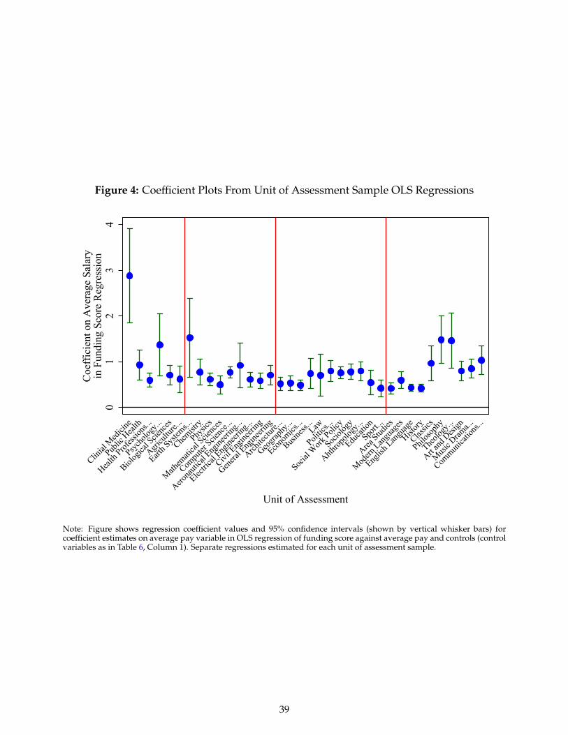
Figure 4: Coefficient Plots From Unit of Assessment Sample OLS Regressions

01

23

4

Coe

ffic

ient

on

Ave

rage

Sal

ary

in F

undi

ng S

core

Reg

ress

ion

Clinial

Med

icine

Public

Heal

th

Health

Profess

ions...

Psycho

logy..

.

Biolog

ical S

cienc

es

Agricu

lture.

..

Earth S

ystem

s...

Chemist

ry

Physic

s

Mathem

atical

Scienc

es

Compu

ter Scie

nce..

.

Aerona

utical

Engine

ering

...

Electric

al Eng

ineeri

ng...

Civil E

ngine

ering

Genera

l Eng

ineeri

ng

Archite

cture.

..

Geogra

phy..

.

Econo

mics...

Busine

ss...Law

Politic

s...

Social

Work

Policy

Sociol

ogy

Ahthrop

ology

...

Educat

ion

Sport..

.

Area Stud

ies

Modern

Langu

ages

Englis

h Lan

guag

e

History

Classic

s

Philoso

phy

Theolo

gy...

Art and

Desi

gn

Music D

rama..

.

Commun

icatio

ns...

Unit of Assessment

Note: Figure shows regression coefficient values and 95% confidence intervals (shown by vertical whisker bars) forcoefficient estimates on average pay variable in OLS regression of funding score against average pay and controls (controlvariables as in Table 6, Column 1). Separate regressions estimated for each unit of assessment sample.

39

Figure 5: Distributions of Grade Point Average and Research Power Across Units and WithinMatched Pairs

(A) Distributions in the Main Sample

05

1015

Den

sity

(%)

1 1.5 2 2.5 3 3.5 4GPA Score

05

1015

20D

ensi

ty (%

)

1 2 3 4 5 6Log REF FTE

(B) Distributions of Within-Cell Differences

010

2030

Den

sity

(%)

-1 -0.5 0 0.5 1Within-Cell Difference in GPA Score

05

1015

2025

Den

sity

(%)

-2 -1 0 1 2Within Cell Difference in Log REF FTE

40

Figure 6: Distributions of Log Funding Score Across Units and Within Matched Pairs

(A) Distributions in the Main Sample0

510

Den

sity

(%)

0 2 4 6 8Log Funding Score

(B) Distributions of Within-Cell Differences

010

2030

40D

ensi

ty (%

)

-.1 -.05 0 .05 .1Within-Cell Difference in Log Funding Score

41

AppendixA Classification of UK Universities by TypesThis appendix lists the members of the University ’Type’ Groups used in the analysis (excludingtherefore institutions with fewer than three professors, or which did not make a submission to theREF, and the London Business School). These groupings are based on the membership of Universityassociations during the relevant period. For each institution, we give in brackets the number ofpanels to which a submission was made, the fulltime equivalent number of staff submitted, and thefulltime equivalent number of full professors in post in October 2013.

Russell Group: In 1994 a group of 17 ’research intensive’ UK universities formed an associationknown as the ’Russell Group’, which grew to 20 Universities by 2006. In 2012 four additionaluniversities joined from the newly-defunct ’1994’ group. Our classification of ’Russell Group’ usesthe 20 members from 2006 onwards on the basis that this group represents long-running coremembers.

University of Birmingham (29, 990, 411)University of Bristol (26, 981, 487)University of Cambridge (28, 1874, 711)University of Leeds (26, 1015, 428)University of Liverpool (16, 584, 253)Imperial College, London (10, 1071, 612)King’s College London (19, 861, 496)London School of Economics (12, 490, 249)University College London (29, 2059, 902)University of Newcastle-upon-Tyne (24, 809, 374)

University of Nottingham (23, 1053, 430)University of Oxford (28, 2264, 905)University of Sheffield (24, 770, 394)University of Southampton (23, 878, 392)University of Warwick (21, 907, 474)University of Edinburgh (28, 1603, 558)University of Glasgow (25, 887, 400)Cardiff University (24, 679, 590)The Queen’s University of Belfast (21, 729, 193)University of Manchester (30, 1426, 780)

The 1994 Group: The ’1994’ Group was also formed in 1994, its membership comprising smallerresearch-intensive universities that had not been invited to join the Russell Group. This groupdisbanded in 2012.

University of Bath (11, 414, 137)University of Durham (20, 629, 250)University of East Anglia (16, 353, 150)University of Essex (10, 304, 131)University of Exeter (19, 621, 230)University of Lancaster (14, 503, 173)University of Leicester (19, 576, 237)Birkbeck College (11, 254, 92)Queen Mary University of London (16, 556, 326)

Royal Holloway and Bedford (16, 360, 182)School of Oriental and African Studies (8, 134, 78)Loughborough University (13, 544, 154)University of Reading (20, 537, 223)University of Surrey (11, 362, 103)University of Sussex (18, 443, 175)University of York (23, 628, 264)University of St Andrews (18, 498, 205)

“New” Universities: This group comprises institutions which were given status as universitiesfrom 1992 onwards. Prior to that time most of the members of this group were known as ‘polytechnics’and delivered mainly post-high school technical education.

A1

Buckinghamshire New University (1, 7, 6)University of Chester (4, 45, 19)Canterbury Christ Church University (2, 36, 8)Edge Hill University (4, 55, 13)Falmouth University (2, 50, 7)Harper Adams University (1, 17, 3)University of Winchester (1, 12, 4)Liverpool Hope University (3, 38, 18)University of Bedfordshire (7, 111, 47)University of Northampton (1, 13, 3)Roehampton University (6, 74, 34)University of Worcester (1, 10, 3)Anglia Ruskin University (5, 55, 35)Bath Spa University (2, 26, 19)Bournemouth University (4, 80, 35)University of Brighton (6, 145, 29)Birmingham City University (8, 98, 42)University of Gloucestershire (4, 37, 15)Coventry University (3, 44, 16)University of East London (6, 78, 27)University of Greenwich (3, 41, 12)University of Hertfordshire (8, 138, 39)University of Lincoln (9, 92, 34)Kingston University (7, 115, 46)Leeds Beckett University (5, 116, 31)

Liverpool John Moores University (9, 138, 47)Manchester Metropolitan University (7, 220, 35)Middlesex University (9, 257, 80)De Montfort University (7, 136, 49)Nottingham Trent University (7, 118, 58)Oxford Brookes University (12, 204, 66)University of Plymouth (13, 295, 101)University of Portsmouth (5, 109, 25)Sheffield Hallam University (7, 139, 37)London South Bank University (1, 34, 4)Teesside University (1, 16, 6)University of West London (3, 29, 13)University of the West of England (8, 192, 72)University of Chichester (1, 8, 3)University of Wolverhampton (7, 119, 37)Cardiff Metropolitan University (2, 23, 9)University of South Wales (4, 37, 16)University of Abertay Dundee (1, 14, 3)Queen Margaret University, Edinburgh (1, 8, 5)Robert Gordon University (2, 20, 10)Glasgow Caledonian University (5, 108, 41)Edinburgh Napier University (5, 65, 28)University of Ulster (14, 311, 123)London Metropolitan University (2, 17, 9)

Specialists: This group comprises a set of high specialised universities offering a limited range ofsubjects including, in some cases, universities offering only a single subject.

Royal College of Art (1, 60, 7)University of the Arts, London (1, 110, 27)Royal Academy of Music (1, 14, 4)Royal Northern College of Music (1, 11, 5)Royal Veterinary College (1, 103, 33)

St George’s Hospital Medical School (1, 44, 41)London School of Hygiene and Tropical Medicine (1,57, 66)University for the Creative Arts (1, 21, 7)Guildhall School of Music and Drama (1, 16, 105)

Others: Universities not included in any of the above groups are assigned to this ’other’ group.

The Open University (12, 325, 96)Cranfield University (3, 224, 50)University of Central Lancashire (11, 201, 52)University of Huddersfield (10, 144, 61)University of Westminster (8, 138, 53)Aston University (5, 164, 45)University of Bradford (4, 93, 44)Brunel University London (15, 452, 97)

City University (10, 316, 141)University of Hull (10, 244, 54)University of Keele (13, 239, 71)University of Kent (18, 500, 135)Goldsmiths College (10, 210, 82)University of Salford (8, 185, 71)University of Strathclyde (14, 508, 174)University of Aberdeen (19, 475, 236)

A2

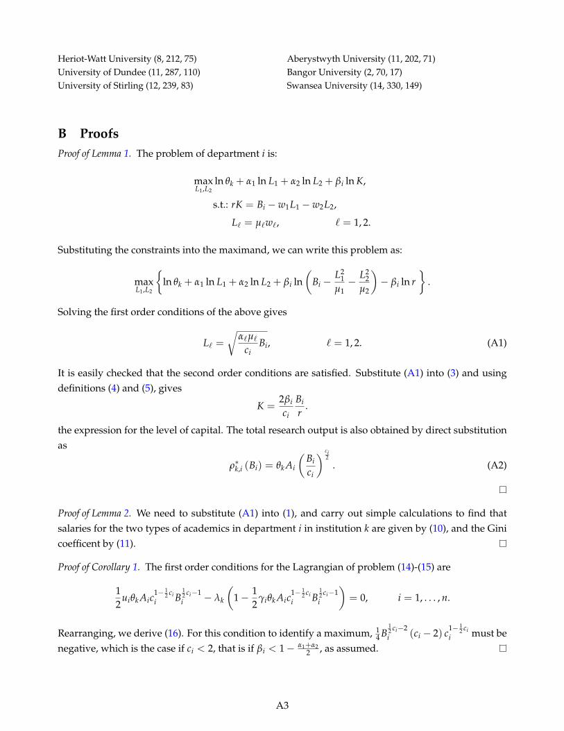
Heriot-Watt University (8, 212, 75)University of Dundee (11, 287, 110)University of Stirling (12, 239, 83)

Aberystwyth University (11, 202, 71)Bangor University (2, 70, 17)Swansea University (14, 330, 149)

B ProofsProof of Lemma 1. The problem of department i is:

maxL1,L2

ln θk + α1 ln L1 + α2 ln L2 + βi ln K,

s.t.: rK = Bi − w1L1 − w2L2,

L` = µ`w`, ` = 1, 2.

Substituting the constraints into the maximand, we can write this problem as:

maxL1,L2

{ln θk + α1 ln L1 + α2 ln L2 + βi ln

(Bi −

L21

µ1− L2

2µ2

)− βi ln r

}.

Solving the first order conditions of the above gives

L` =

√α`µ`

ciBi, ` = 1, 2. (A1)

It is easily checked that the second order conditions are satisfied. Substitute (A1) into (3) and usingdefinitions (4) and (5), gives

K =2βi

ci

Bi

r.

the expression for the level of capital. The total research output is also obtained by direct substitutionas

ρ∗k,i (Bi) = θk Ai

(Bi

ci

) ci2

. (A2)

Proof of Lemma 2. We need to substitute (A1) into (1), and carry out simple calculations to find thatsalaries for the two types of academics in department i in institution k are given by (10), and the Ginicoefficent by (11).

Proof of Corollary 1. The first order conditions for the Lagrangian of problem (14)-(15) are

12

uiθk Aic1− 1

2 cii B

12 ci−1i − λk

(1− 1

2γiθk Aic

1− 12 ci

i B12 ci−1i

)= 0, i = 1, . . . , n.

Rearranging, we derive (16). For this condition to identify a maximum, 14 B

12 ci−2i (ci − 2) c1− 1

2 cii must be

negative, which is the case if ci < 2, that is if βi < 1− α1+α22 , as assumed.

A3

C Additional tables and figures

Table A1: Summary Statistics Departmental Level REF Performance by Component

mean sd min max

Overall % 4* 26.88 14.66 0.00 79.00

Overall % 3* 47.46 11.89 3.00 83.00

Overall % 2* 21.95 12.08 0.00 75.00

Overall % 1* 3.23 5.23 0.00 55.00

Overall % 0* 0.48 1.29 0.00 10.00

Outputs % 4* 21.79 11.24 0.00 69.70

Outputs % 3* 48.44 12.23 0.00 100.00

Outputs % 2* 25.44 12.05 0.00 72.90

Outputs % 1* 3.82 5.68 0.00 60.60

Outputs % 0* 0.50 1.15 0.00 10.30

Environment % 4* 34.03 33.46 0.00 100.00

Environment % 3* 47.83 27.50 0.00 100.00

Environment % 2* 16.39 23.39 0.00 100.00

Environment % 1* 1.73 8.32 0.00 90.00

Environment % 0* 0.03 0.81 0.00 25.00

Impact % 4* 38.00 28.04 0.00 100.00

Impact % 3* 43.98 22.94 0.00 100.00

Impact % 2* 14.93 19.48 0.00 100.00

Impact % 1* 2.32 8.26 0.00 90.00

Impact % 0* 0.77 4.82 0.00 40.00

Note: Sample size = 1093 departments submitted to REF 2014. For explanation of REF performance measures see maintext.

A4

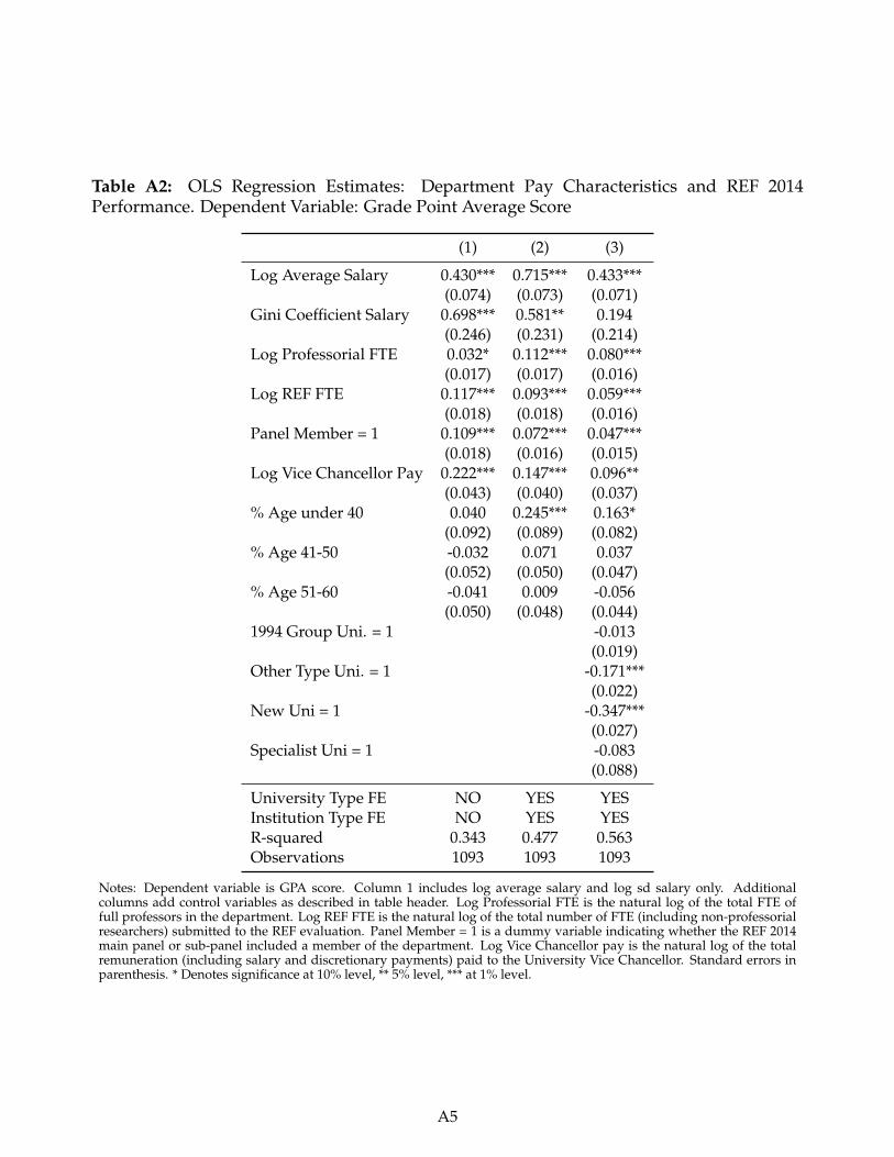
Table A2: OLS Regression Estimates: Department Pay Characteristics and REF 2014Performance. Dependent Variable: Grade Point Average Score

(1) (2) (3)

Log Average Salary 0.430*** 0.715*** 0.433***(0.074) (0.073) (0.071)

Gini Coefficient Salary 0.698*** 0.581** 0.194(0.246) (0.231) (0.214)

Log Professorial FTE 0.032* 0.112*** 0.080***(0.017) (0.017) (0.016)

Log REF FTE 0.117*** 0.093*** 0.059***(0.018) (0.018) (0.016)

Panel Member = 1 0.109*** 0.072*** 0.047***(0.018) (0.016) (0.015)

Log Vice Chancellor Pay 0.222*** 0.147*** 0.096**(0.043) (0.040) (0.037)

% Age under 40 0.040 0.245*** 0.163*(0.092) (0.089) (0.082)

% Age 41-50 -0.032 0.071 0.037(0.052) (0.050) (0.047)

% Age 51-60 -0.041 0.009 -0.056(0.050) (0.048) (0.044)

1994 Group Uni. = 1 -0.013(0.019)

Other Type Uni. = 1 -0.171***(0.022)

New Uni = 1 -0.347***(0.027)

Specialist Uni = 1 -0.083(0.088)

University Type FE NO YES YESInstitution Type FE NO YES YESR-squared 0.343 0.477 0.563Observations 1093 1093 1093

Notes: Dependent variable is GPA score. Column 1 includes log average salary and log sd salary only. Additionalcolumns add control variables as described in table header. Log Professorial FTE is the natural log of the total FTE offull professors in the department. Log REF FTE is the natural log of the total number of FTE (including non-professorialresearchers) submitted to the REF evaluation. Panel Member = 1 is a dummy variable indicating whether the REF 2014main panel or sub-panel included a member of the department. Log Vice Chancellor pay is the natural log of the totalremuneration (including salary and discretionary payments) paid to the University Vice Chancellor. Standard errors inparenthesis. * Denotes significance at 10% level, ** 5% level, *** at 1% level.

A5

Table A3: OLS Regression Estimates by Main Panel (Grade Point Average Score)

(1) (2) (3) (4)Panel A Panel B Panel C Panel D

Medicine Science & Social Arts &Engineering Sciences Humanities

Log Average Salary 0.753*** 0.482*** 0.422*** 0.756***(0.201) (0.154) (0.126) (0.134)

Gini Coefficient Salary 1.204* 1.066** 0.090 0.451(0.566) (0.432) (0.440) (0.483)

Log Professorial FTE -0.038 0.163*** 0.019 0.115***(0.030) (0.036) (0.031) (0.034)

Log REF FTE 0.122*** 0.032 0.208*** 0.015(0.037) (0.038) (0.033) (0.033)

Panel Member = 1 0.080* 0.080** 0.124*** 0.106***(0.042) (0.033) (0.031) (0.031)

Log Vice Chancellor Pay 0.219* 0.177* 0.237*** 0.115(0.106) (0.082) (0.076) (0.072)

% Age under 40 -0.074 0.417* 0.167 0.068(0.256) (0.212) (0.141) (0.168)

% Age 41-50 0.056 -0.006 0.098 -0.052(0.143) (0.109) (0.091) (0.083)

% Age 51-60 0.046 -0.121 0.074 -0.073(0.128) (0.113) (0.089) (0.078)

University Type FE YES YES YES YESR-squared 0.418 0.497 0.398 0.320Observations 183 263 369 278

Note: Dependent variable is GPA score. OLS regression estimated on four mutually exclusive samples of academicdepartments categorised by REF Main Panel. Log Professorial FTE is the natural log of the total FTE of full professorsin the department. Log REF FTE is the natural log of the total number of FTE (including non-professorial researchers)submitted to the REF evaluation. Panel Member = 1 is a dummy variable indicating whether the REF 2014 main panelor sub-panel included a member of the department. Log Vice Chancellor pay is the natural log of the total remuneration(including salary and discretionary payments) paid to the University Vice Chancellor. Standard errors in parenthesis. *Denotes significance at 10% level, ** 5% level, *** at 1% level.

A6

Table A4: OLS Regression Estimates Omitting Medicine UOA

(1) (2)Funding Score GPA Score

Log Average Salary 0.497*** 0.426***(0.092) (0.072)

Gini Coefficient Salary 0.530* 0.155(0.276) (0.217)

Log Professorial FTE 0.111*** 0.080***(0.021) (0.016)

Log REF FTE 1.058*** 0.064***(0.021) (0.017)

Panel Member = 1 0.061*** 0.049***(0.020) (0.016)

Log Vice Chancellor Pay 0.109* 0.090**(0.048) (0.038)

% Age under 40 0.222* 0.163*(0.104) (0.082)

% Age 41-50 0.050 0.032(0.060) (0.047)

% Age 51-60 -0.059 -0.061(0.056) (0.044)

1994 Group Uni. = 1 -0.027 -0.015(0.024) (0.019)

Other Type Uni. = 1 -0.207*** -0.172***(0.028) (0.022)

New Uni = 1 -0.420*** -0.351***(0.034) (0.027)

Specialist Uni = 1 -0.118 -0.108(0.133) (0.104)

Unit of Assessment FE YES YESUniversity Type FE YES YESR-squared 0.906 0.565Observations 1067 1067

Note: Dependent variable is the natural log of the Funding Score in Column 1 and the natural log of the GPA score inColumn 2. OLS regressions estimated on the main sample minus departments in the Medicine Unit of Assessment. LogProfessorial FTE is the natural log of the total FTE of full professors in the department. Log REF FTE is the natural log ofthe total number of FTE (including non-professorial researchers) submitted to the REF evaluation. Panel Member = 1 isa dummy variable indicating whether the REF 2014 main panel or sub-panel included a member of the department. LogVice Chancellor pay is the natural log of the total remuneration (including salary and discretionary payments) paid to theUniversity Vice Chancellor. Standard errors in parenthesis. * Denotes significance at 10% level, ** 5% level, *** at 1% level.

A7

Table A5: Difference-in-Difference Estimates of Effects of REF 2014 Funding Score onChanges in Departmental Wage Structure, 2013 - 2016 (Full Samples of Matches)

(1) (2) (3) (4)Change Log Change Log Change Change TotalMean Salary Top Quartile Wage Bill Gini Coeff. FTE Professors

Funding Score 0.002 -0.028 0.005 1.001(0.005) (0.119) (0.004) (0.758)

% Age under 40 -0.053 2.642*** 0.021 6.970***(0.037) (0.895) (0.017) (1.950)

% Age 41-50 -0.032* 0.245 -0.011 1.144(0.017) (0.423) (0.008) (0.921)

% Age 51-60 -0.001 0.403 -0.007 -0.087(0.016) (0.393) (0.007) (0.855)

Log REF FTE -0.002 0.050 -0.003 -0.525(0.007) (0.169) (0.003) (0.368)

Main Panel FE YES YES YES YESR-squared 0.013 0.016 0.019 0.068Observations 562 562 562 562

Note: Table shows OLS estimates from difference-in-difference models based on Equation 22. The dependent variableand funding score variables are the differenced variables, calculated as the differences between matched pairs (by GPAand FTE) in the first-differences in the variables between 2013 and 2015. Other control variables are differences betweenthe matched departments in levels measured in the 2013 data. * Denotes significance at 10% level, ** 5% level, *** at 1%level.

A8

Table A6: Difference-in-Difference Estimates of Effects of REF 2014 GPA on Changes inDepartmental Wage Structure, 2013 - 2016 (Full Samples of Matches)

(1) (2) (3) (4)Change Log Change Log Change Change TotalMean Salary Top Quartile Wage Bill Gini Coeff. FTE Professors

GPA Score -0.073 0.067*** 0.011 6.226***(0.098) (0.023) (0.011) (1.173)

% Age under 40 0.859 -0.091*** 0.012 4.540***(0.895) (0.034) (0.016) (1.756)

% Age 41-50 0.294 -0.007 0.002 1.656*(0.437) (0.017) (0.008) (0.857)

% Age 51-60 0.647 0.005 0.002 -0.614(0.431) (0.016) (0.008) (0.845)

Log REF FTE 0.073 0.012* 0.002 -0.604*(0.140) (0.005) (0.002) (0.276)

Main Panel FE YES YES YES YESR-squared 0.008 0.031 0.004 0.039Observations 571 571 571 571

Note: Table shows OLS estimates from difference-in-difference models based on Equation 22. The dependent variable andfunding score variables are the differenced variables, calculated as the differences between matched pairs (by FundingScore) in the first-differences in the variables between 2013 and 2015. Other control variables are differences between thematched departments in levels measured in the 2013 data. * Denotes significance at 10% level, ** 5% level, *** at 1% level.

A9

Table A7: OLS Regression Estimates: Department Pay Characteristics and REF 2014Performance. Dependent Variable: Grade Point Average Score

(1) (2) (3)

Log Average Salary 0.435*** 0.728*** 0.444***(0.074) (0.073) (0.071)

Gini Coefficient Salary 0.678*** 0.552** 0.176(0.246) (0.230) (0.213)

Log Professorial FTE 0.034* 0.116*** 0.083***(0.017) (0.017) (0.016)

Log REF FTE 0.116*** 0.091*** 0.057***(0.018) (0.017) (0.016)

Panel Member = 1 0.107*** 0.068*** 0.044***(0.018) (0.016) (0.015)

Log Vice Chancellor Pay 0.226*** 0.155*** 0.099***(0.043) (0.040) (0.037)

% Age under 40 0.042 0.251*** 0.168*(0.092) (0.088) (0.081)

% Age 41-50 -0.028 0.078 0.043(0.052) (0.050) (0.046)

% Age 51-60 -0.044 0.007 -0.057(0.050) (0.047) (0.044)

Proportion PT Staff 0.100* 0.174*** 0.122**(0.055) (0.051) (0.048)

1994 Group Uni. = 1 -0.020(0.019)

Other Type Uni. = 1 -0.169***(0.022)

New Uni = 1 -0.346***(0.027)

Specialist Uni = 1 -0.097(0.088)

R-squared 0.345 0.482 0.565Observations 1093 1093 1093

Notes: Dependent variable is GPA score. Column 1 includes log average salary and log sd salary only. Additionalcolumns add control variables as described in table header. Standard errors in parenthesis. Log Professorial FTE is thenatural log of the total FTE of full professors in the department. Log REF FTE is the natural log of the total number ofFTE (including non-professorial researchers) submitted to the REF evaluation. Panel Member = 1 is a dummy variableindicating whether the REF 2014 main panel or sub-panel included a member of the department. Log Vice Chancellorpay is the natural log of the total remuneration (including salary and discretionary payments) paid to the University ViceChancellor. Standard errors in parenthesis. * Denotes significance at 10% level, ** 5% level, *** at 1% level.

A10

Table A8: OLS Regression Estimates: Department Pay Characteristics and REF 2014Performance. Dependent Variable: Log REF Funding Score

(1) (2) (3)

Log Average Salary 0.500*** 0.858*** 0.524***(0.096) (0.092) (0.091)

Gini Coefficient Salary 0.891*** 0.996*** 0.546*(0.317) (0.289) (0.271)

Log Professorial FTE 0.039* 0.154*** 0.114***(0.021) (0.022) (0.020)

Log REF FTE 1.115*** 1.089*** 1.048***(0.023) (0.022) (0.021)

Panel Member = 1 0.140*** 0.085*** 0.056***(0.023) (0.021) (0.019)

Log Vice Chancellor Pay 0.285*** 0.188*** 0.121**(0.055) (0.050) (0.047)

% Age under 40 -0.012 0.326*** 0.229*(0.118) (0.111) (0.104)

% Age 41-50 -0.115* 0.105* 0.065(0.067) (0.063) (0.059)

% Age 51-60 -0.085 0.021 -0.054(0.064) (0.060) (0.056)

Proportion PT Staff 0.114 0.209*** 0.150**(0.071) (0.064) (0.061)

1994 Group Uni. = 1 -0.032(0.024)

Other Type Uni. = 1 -0.203***(0.028)

New Uni = 1 -0.414***(0.034)

Specialist Uni = 1 -0.089(0.112)

Unit of Assessment FE NO YES YESUniversity Type FE NO NO YESR-squared 0.867 0.899 0.913Observations 1093 1093 1093

Notes: Dependent variable is natural log of the research funding score. Column 1 includes log average salary and logsd salary only. Standard errors in parenthesis. Log Professorial FTE is the natural log of the total FTE of full professorsin the department. Log REF FTE is the natural log of the total number of FTE (including non-professorial researchers)submitted to the REF evaluation. Panel Member = 1 is a dummy variable indicating whether the REF 2014 main panelor sub-panel included a member of the department. Log Vice Chancellor pay is the natural log of the total remuneration(including salary and discretionary payments) paid to the University Vice Chancellor. Standard errors in parenthesis. *Denotes significance at 10% level, ** 5% level, *** at 1% level.

A11

Table A9: Difference-in-Difference Estimates of Effects of REF 2014 Funding Score at MainPanel Level on Changes in Departmental Wage Structure, 2013 - 2016

(1) (2) (3) (4)Change Log Change Log Change Change TotalMean Salary Top Quartile Wage Bill Gini Coeff. FTE Professors

Main Panel FS (Incl. Dept) 0.000 -0.010 0.000 -0.025(0.000) (0.008) (0.000) (0.017)

% Age under 40 -0.010 1.680 0.023 8.009***(0.059) (1.317) (0.023) (2.766)

% Age 41-50 -0.049* 0.776 -0.006 0.856(0.028) (0.622) (0.011) (1.306)

% Age 51-60 0.004 0.283 -0.003 -0.503(0.025) (0.553) (0.010) (1.161)

Log REF FTE -0.005 0.499 -0.002 0.040(0.015) (0.330) (0.006) (0.692)

Main Panel FE YES YES YES YESR-squared 0.022 0.018 0.007 0.056Observations 269 269 269 269

Note: Table shows OLS estimates from difference-in-difference models based on Equation 22. The dependent variable andfunding score variables are the differenced variables, calculated as the differences between matched pairs (by GPA andFTE) in the first-differences in the variables between 2013 and 2015. In this regression the Funding Score is differences atthe level of the Main Panel. Other control variables are differences between the matched departments in levels measuredin the 2013 data. * Denotes significance at 10% level, ** 5% level, *** at 1% level.

A12

Table A10: Difference-in-Difference Estimates of Effects of REF 2014 GPA at Main Panel Levelon Changes in Departmental Wage Structure, 2013 - 2016

(1) (2) (3) (4)Change Log Change Log Change Change TotalMean Salary Top Quartile Wage Bill Gini Coeff. FTE Professors

Faculty GPA Score (Incl. Dept) -2.646 0.028 -0.013 4.633(2.530) (0.103) (0.046) (5.477)

% Age under 40 0.194 -0.030 0.030 1.584(1.321) (0.054) (0.024) (2.859)

% Age 41-50 -0.575 -0.005 -0.003 0.058(0.645) (0.026) (0.012) (1.397)

% Age 51-60 1.034 0.011 -0.002 -1.097(0.646) (0.026) (0.012) (1.398)

Log REF FTE -0.184 0.014 -0.002 0.214(0.215) (0.009) (0.004) (0.466)

R-squared 0.041 0.013 0.009 0.011Observations 258 258 258 258

Note: Table shows OLS estimates from difference-in-difference models based on Equation 22. The dependent variable andfunding score variables are the differenced variables, calculated as the differences between matched pairs (by FundingScore) in the first-differences in the variables between 2013 and 2015. In this regression the GPA Score is differences at thelevel of the Main Panel. Other control variables are differences between the matched departments in levels measured inthe 2013 data. * Denotes significance at 10% level, ** 5% level, *** at 1% level.

A13

Table A11: Difference-in-Difference Estimates of Effects of REF 2014 GPA on Changes inDepartmental Wage Structure by REF Main Panel, 2013 - 2016. Sample of All Matches

(1) (2) (3) (4)Change Log Change Log Change Change TotalMean Salary Top Quartile Wage Bill Gini Coeff. FTE Professors

Main Panel A: MedicineDept GPA Score -2.084 -0.029 -0.051 9.009***

(2.073) (0.081) (0.036) (1.895)

R-squared 0.119 0.068 0.039 0.069Observations 102 102 102 102

Main Panel B: Science & EngineeringDept GPA Score 0.779 0.095** 0.030 5.364

(1.265) (0.069) (0.026) (3.103)

R-squared 0.021 0.058 0.068 0.077Observations 143 143 143 143

Main Panel C: Social SciencesDept GPA Score 0.935 0.097*** -0.019 4.813***

(1.672) (0.017) (0.039) (1.316)

R-squared 0.014 0.055 0.018 0.066Observations 169 169 169 169

Main Panel D: Arts & HumanitiesDept GPA Score -2.047 -0.105 0.004 -1.873

(2.159) (0.077) (0.037) (3.485)

R-squared 0.063 0.096 0.033 0.062Observations 127 127 127 127

Note: Table shows OLS estimates from difference-in-difference models based on Equation 22. The dependent variable andfunding score variables are the differenced variables, calculated as the differences between matched pairs (by FundingScore) in the first-differences in the variables between 2013 and 2015. Samples divided by REF 2014 Main Panel. Othercontrol variables are differences between the matched departments in levels measured in the 2013 data. * Denotessignificance at 10% level, ** 5% level, *** at 1% level.

A14

Figure A1: Correlation Between Mean Pay and GPA Score

(A) By REF Main Panel

12

34

Gra

de P

oint

Ave

rage

, REF

201

4

50 60 70 80 90 100 110 120 130Mean Professorial Salary

Panel A Medicine

12

34

Gra

de P

oint

Ave

rage

, REF

201

4

50 60 70 80 90 100 110 120 130Mean Professorial Salary

Panel B Science & Engineering1

23

4G

rade

Poi

nt A

vera

ge, R

EF 2

014

50 60 70 80 90 100 110 120 130Mean Professorial Salary

Panel C Social Science

12

34

Gra

de P

oint

Ave

rage

, REF

201

4

50 60 70 80 90 100 110 120 130Mean Professorial Salary

Panel D Arts & Humanities

(B) By University Type

12

34

Gra

de P

oint

Ave

rage

, REF

201

4

50 60 70 80 90 100 110 120 130Mean Professorial Salary

Russell Group

12

34

Gra

de P

oint

Ave

rage

, REF

201

4

50 60 70 80 90 100 110 120 130Mean Professorial Salary

1994 Group

12

34

Gra

de P

oint

Ave

rage

, REF

201

4

50 60 70 80 90 100 110 120 130Mean Professorial Salary

Others

12

34

Gra

de P

oint

Ave

rage

, REF

201

4

50 60 70 80 90 100 110 120 130Mean Professorial Salary

New

Note: Each observation represents an individual academic department. Figure show scatter plots and fitted regressionlines. Observations grouped by REF Main Panel (Plot group A) and University Type (Plot group B).

A15

Figure A2: Correlation Between Gini Pay and GPA Score

(A) By REF Main Panel

12

34

Gra

de P

oint

Ave

rage

, REF

201

4

0 .1 .2 .3 .4Gini Coefficient Professorial Salary

Panel A Medicine

12

34

Gra

de P

oint

Ave

rage

, REF

201

4

0 .1 .2 .3 .4Gini Coefficient Professorial Salary

Panel B Science & Engineering1

23

4G

rade

Poi

nt A

vera

ge, R

EF 2

014

0 .1 .2 .3 .4Gini Coefficient Professorial Salary

Panel C Social Science

12

34

Gra

de P

oint

Ave

rage

, REF

201

4

0 .1 .2 .3 .4Gini Coefficient Professorial Salary

Panel D Arts & Humanities

(B) By University Type

12

34

Gra

de P

oint

Ave

rage

, REF

201

4

0 .1 .2 .3 .4Gini Coefficient Professorial Salary

Russell Group

12

34

Gra

de P

oint

Ave

rage

, REF

201

4

0 .1 .2 .3 .4Gini Coefficient Professorial Salary

1994 Group

12

34

Gra

de P

oint

Ave

rage

, REF

201

4

0 .1 .2 .3 .4Gini Coefficient Professorial Salary

Others

12

34

Gra

de P

oint

Ave

rage

, REF

201

4

0 .1 .2 .3 .4Gini Coefficient Professorial Salary

New

Note: Each observation represents an individual academic department. Figure show scatter plots and fitted regressionlines. Observations grouped by REF Main Panel (Plot group A) and University Type (Plot group B).

A16

Figure A3: Vice Chancellor Pay and Funding Score Performance

Nottingham Trent

Oxford

02

46

810

Log

Uni

vers

ity T

otal

Fun

ding

Sco

re, R

EF 2

014

100 200 300 400 500 600Vice Chancellor Total Remuneration

Note: Each observation corresponds to an individual university. Figure shows a scatter plot of total remuneration ofuniversity vice chancellors (x-axis, including pension contributions and discretionary payments) and log funding score (y-axis). The red fitted regression line is estimated on all observations; the blue fitted regression line is fitted on observationsexcluding the far-right outlier value.

A17