abstract - university of virginia

2

Abstract

The Eastern Oyster (Crassostrea virginica) once played a pivotal ecological role

in Virginia waters and the Chesapeake Bay. However, unregulated over-harvesting,

combined with reduced water quality and disease, has caused a drastic decline in oyster

populations, such that present day levels are less than 2% of pre-harvest populations.

Restoration efforts, currently underway to re-establish healthy oyster populations, are

focused on rehabilitating benthic habitat to be suitable for natural oyster larval

recruitment and growth. The goal of this study was to understand the hydrodynamics

involved in fluid and sediment transport over reefs, and how these dynamics may impact

larval transport to healthy and restored reef areas.

Velocity and turbulence data was collected off of the Eastern shore of Virginia

over multiple benthic surfaces including a mud flat, a healthy reef, and two restoration

sites comprised of either fossil oyster or whelk shell. Reynolds stresses, shear velocity,

u*, and drag coefficients, CD, were computed and due to the extreme roughness of the

reef, mean estimates of u* over a healthy reef were found to be 47% greater than those

found over a restoration site. Enhanced shear increased both turbulent mixing and drag

above the reef, but within the interstitial areas between individual oysters, mean

velocities and turbulent motions were reduced. CD, used as a measure of roughness, also

increased with elevation on the healthy reef.

Small-scale hydrodynamic forces were studied in an open-channel, recirculating,

water flume along benthic roughnesses of varying height and spacing, used to mimic

3

variability found on the reef. Drag and lift forces within the structure decreased with

increasing height and increased with increased spacing. Geometrically similar slate tile

structures were deployed in the field over a five month period, and the greatest larval

recruitment corresponded closely to locations where drag and lift forces were reduced.

The combined field and laboratory data suggests that restoration efforts should consider

both elevation and bed roughness similar to those found on healthy oyster reefs, to

provide suitable hydrodynamic conditions that promote larval recruitment, prevent burial

by sediment, and may provide some refuge from predation.

4

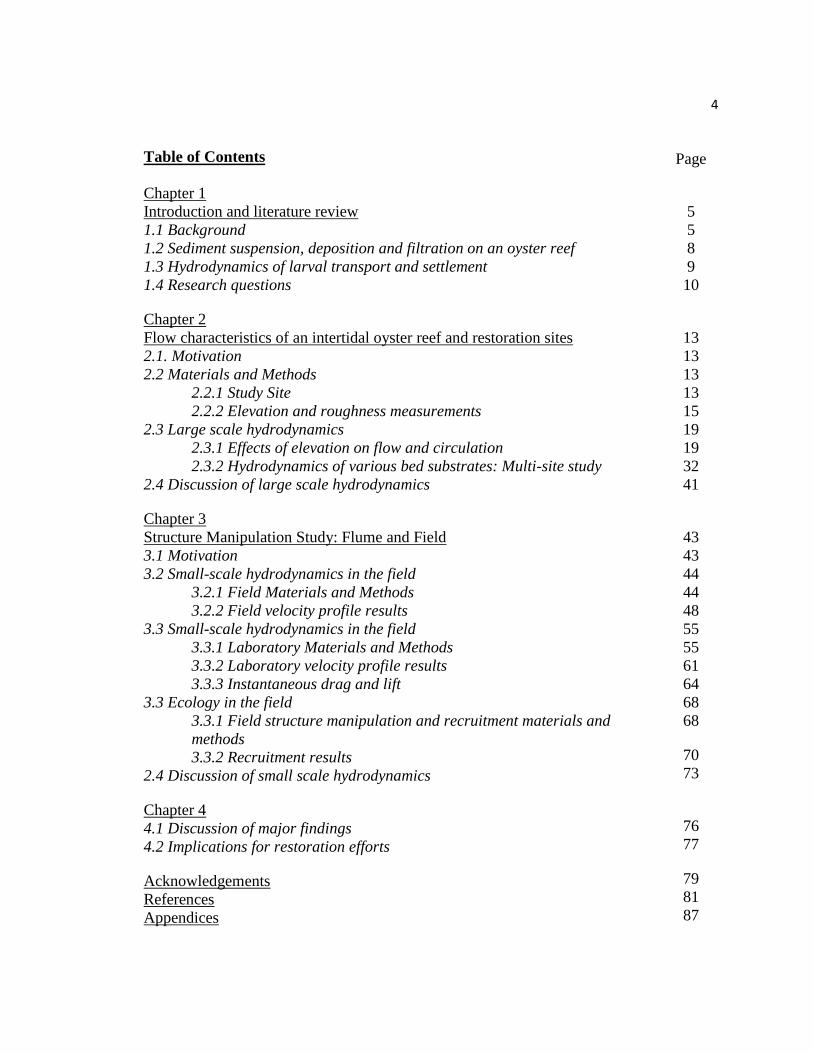
Table of Contents

Chapter 1

Introduction and literature review

1.1 Background

1.2 Sediment suspension, deposition and filtration on an oyster reef

1.3 Hydrodynamics of larval transport and settlement

1.4 Research questions

Chapter 2

Flow characteristics of an intertidal oyster reef and restoration sites

2.1. Motivation

2.2 Materials and Methods

2.2.1 Study Site

2.2.2 Elevation and roughness measurements

2.3 Large scale hydrodynamics

2.3.1 Effects of elevation on flow and circulation

2.3.2 Hydrodynamics of various bed substrates: Multi-site study

2.4 Discussion of large scale hydrodynamics

Chapter 3

Structure Manipulation Study: Flume and Field

3.1 Motivation

3.2 Small-scale hydrodynamics in the field

3.2.1 Field Materials and Methods

3.2.2 Field velocity profile results


3.3.1 Laboratory Materials and Methods

3.3.2 Laboratory velocity profile results

3.3.3 Instantaneous drag and lift

3.3 Ecology in the field

3.3.1 Field structure manipulation and recruitment materials and

methods

3.3.2 Recruitment results

2.4 Discussion of small scale hydrodynamics

Chapter 4

4.1 Discussion of major findings

4.2 Implications for restoration efforts

Acknowledgements

References

Appendices

Page

5

5

8

9

10

13

13

13

13

15

19

19

32

41

43

43

44

44

48

55

55

61

64

68

68

70

73

76

77

79

81

87

5

Chapter 1

Introduction and literature review

1.1 Background

The Eastern Oyster (Crassostrea virginica) can be found from as far south as

Argentina to as far north as the Gulf of St. Lawrence in Canada where they inhabit

estuaries and coastal waters (Carriker and Gaffney 1996). With their historical prevalence

and subsequent decades of decline in Virginia waters and Chesapeake Bay, their role in

physical-biological coupling (Lenihan, 1999) and in local ecosystem services (Nelson et

al., 2004) has come into the spotlight. Fish and many invertebrates use oyster reefs as

foraging grounds, so healthy oyster reefs promote estuarine biodiversity (Arve 1960,

Bahr and Lanier 1981, Zimmerman et al. 1989, Lenihan et al. 1998). As well as

providing historically important benthic substrate and habitat for other species

(McCormick-Ray 1998), oysters are also important to the water quality of the shallow

lagoons where the reefs are located. As filter feeders, they filter algae and detritus from

the water improving both water quality and water clarity and deposit fecal material to the

sea floor, (Newell 1988). There is currently a debate in the literature over the ability of C.

virginica to control phytoplankton blooms in the Chesapeake Bay (Newell 1988,

Pomeroy et al. 2006, Newell et al. 2007, Pomeroy et al. 2007), but their ability to clear

water on a smaller scale and modify their local environment is well documented (e.g.

Nelson et al., 2004; Porter et al., 2004; Cerco and Noel, 2007).

6

Despite the importance of oysters to the local ecosystem, over fishing, disease and

poor management practices have resulted in the loss of 99% of the historical biomass of

C. virginica in the Chesapeake Bay (Rothschild et al. 1994, Kemp et al. 2005). There are

now increased efforts to restore and manage oyster reefs (Rothschild et al. 1994 Cerco

and Noel 2007, Schulte et al. 2009), and agencies such as The Nature Conservancy are

relying on continued research that could provide insight into the parameters that must be

considered to achieve successful restoration. Some of these parameters include disease

susceptibility, predation, and environmental conditions.

Dense concentrations of the filter feeders comprise unharvested oyster reefs

(Figure 1.1) (Dame et al. 1984). Due to reef expansion, both horizontally and vertically

as a result of oysters settling and growing on each other, they affect processes such as

sedimentation (McCormick-Ray 1998) and particulate organic carbon removal by means

of biofiltration as well as physical factors (Dame et al. 1984). For reefs to develop,

oysters must survive a larval phase as planktotrophic larvae extending several weeks

(Loosanoff 1965, Coen et al. 2000), attach to substrata, and grow from spat to large

individuals. C. virginica spawning and growth rates are highest when the water

temperature is around 25°C and vary with temperature ranging 6–32°C (Galtsoff 1964),

and the majority of reefs are intertidal or found in areas of low salinity (<15 ppt) (Coen et

al. 2000). Spawning from year to year is significant not only for continuing recruitment

but the larvae serve as food for other aquatic animals (Loosanoff 1965). Since water

temperature is not controllable on a short time scale, restoration efforts are focused on

7

creating suitable benthic environments for recruitment in which sanctuaries can protect

areas where oysters grow into spawning adults (Brumbaugh et al. 2000).

Figure 1.1: Oyster reef found within the Hillcrest reef tract, a TNC sanctuary (see Figure 2.1)

Recent restoration successes have been seen in sanctuary areas of the Chesapeake

Bay where studies have found that the higher the vertical relief of the oyster reef, the

more successful is the recruitment and growth of oysters (Schulte et al. 2009). Overall, a

five-fold increase in living oyster densities was found, and attributed to the high relief of

the successful oyster reefs. Hydrodynamic conditions over these reefs should be different

than the hydrodynamic conditions over the low relief reefs because of factors such as

water depth and benthic roughness. Lenihan et al. 1996 showed that the growth,

condition and survival of oysters are positively correlated to an increase in flow velocity.

It is reasonable to expect that flow velocities relative to ambient flow velocities would

increase with the vertical relief of an oyster reef. Bartol et al. (1999) discovered that mid-

8

intertidal oysters within reef interstices grow faster and live longer than oysters at the reef

surface, and suggested that factors such as hydrodynamics vary between locations along

the reef.

1.2 Sediment suspension, deposition and filtration on an oyster reef

Directly related to the hydrodynamics of an oyster reef is enhanced sedimentation

due to active filtration of particles in the water column by the oysters and by the presence

of reef structure. Too much sedimentation, however, can prevent larvae from attaching to

shell and juvenile and adult oysters can be smothered. Sedimentation negatively affects

recruitment and growth of oysters in the field, and sedimentation decreases with

increased flow velocities (MacKenzie 1983). Oysters filter water to capture food such as

phytoplankton and they filter sediment out of the water column at the same time. The

sediment and seston the oysters remove from the overlying water column through active

filtration (see Appendix I for preliminary study results) is then deposited on the benthic

surface as pseudo-feces that are dense clumps of fine particles of sediment and organic

material (Haven and Morales-Almo, 1966). Turbulent conditions created by the bed

roughness improve resuspension of fine particles, and slowed flow velocity by the reef

structure promotes sedimentation (Nelson et al., 2004). Sedimentation is seasonally

highest where flow speed is lowest at the bases of the reefs (Lenihan 1999), and

sedimentation quickly covers low-relief reefs. In Lenihan (1999), his study identified the

greater influences on oyster mortality. Macro-predators such as fish and crabs only

accounted for 4-20% of total oyster mortality regardless of reef height, position, or cage

type, whereas oysters at the base of reefs that were susceptible to burial by sediment

9

experienced greater mortality (97 ± 6%) than those on the reef crest (24 ± 9%). This

supports the idea that physical-biological coupling has a great influence on the system.

1.3 Hydrodynamics of larval transport and settlement

Some challenges for oyster recovery efforts are promoting the successful larval

transport to new reef sites, providing accommodating sites for larval settlement, and

maintaining habitat suitable for oyster growth and survival. The topographic roughness

and elevation of a reef are responsible for the local hydrodynamics that can impact the

success of larval settlement and recruitment. Larvae preferentially settle on existing

oyster reefs due to a hard, stable substrate for firm attachment and topographic variability

that prevents burial by sediments. Settlement success has been shown to be dependent

upon their ability to quickly land, attach, and undergo metamorphosis before they are

washed away by fluid stresses, such as lift and drag, or are transferred to areas where they

can be buried by depositing sediments. Shear stress acts tangential to their settlement

surface and it is this shearing force that is capable of preventing settlement or dislodging

the larvae after they settle (Reidenbach et al. 2009). Although previous studies have

shown that benthic shear stresses influence the success of larval settlement (Soniat 2004),

little is known about the actual distributions of shear stresses along oyster beds.

The physical structure of the reef controls physical variables such as flow speed

which then determines the success of the oysters and oyster larvae in that location.

Crimaldi et al. (2002) describes the link between local instantaneous bed shear stresses in

a highly episodic stress record and the probability of successful settlement. This

10

experiment was in a laboratory with a bed of clams set equidistance apart from one

another, and high resolution velocity measurements were used to infer stresses imposed

on settling larvae. Not all of Crimaldi‘s conclusions can be applied to the densely

populated oyster beds because the turbulence described occur between the clams shells

with sufficient distance between each other may not exist in the small interstices between

adult oysters. The observed transport of clam larvae to the bed, however, is likely similar

to that of oyster larvae. Turbulence is not only responsible for the transport of larvae to

the bed but can also be responsible for dislodging the larvae before they are permanently

anchored. Clam larvae must land on the substrate during an adequately long stress lull to

successfully anchor (Crimaldi et al. 2002), and higher Reynolds numbers meant that the

larval fluxes to the bed were much greater. Instantaneous drag forces have been shown to

be more likely to cause larval detachment than the maximum drag forces (Eckman et al.

1990).

1.4 Research questions

Based on the heightened focus on oyster restoration and necessity to defining

parameters that will make restoration efforts more successful this study focuses on the

role hydrodynamics plays in creating an environment that will encourage larval

settlement success. The questions addressed through field research and laboratory flume

experimentation are: (1) How do reef elevation and bed roughness affect shear stresses

and fluid drag in the turbulent boundary layer over an intertidal oyster reef and adjacent

restoration sites; (2) How does shear stress distribution and variability differ among sites

11

of varying topographies; and (3) How might the varying hydrodynamic conditions impact

larval recruitment?

To address the first two questions, which will be discussed in Chapter 2,

instruments were placed at an established oyster reef and adjacent oyster restoration sites

located approximately 1 km offshore from the Anheuser-Busch Coastal Research Center

at the VCR. The oyster site is part of a network of numerous healthy patches of oyster

reefs surrounding an oyster restoration area operated by The Nature Conservancy. Work

was in conjunction with restoration efforts being overseen by Barry Truitt, The Nature

Conservancy (TNC) Director of Science and Stewardship at the VCR. First, the four

study sites were surveyed which are adjacent to one another: the a healthy living reef, a

TNC restoration site where the benthos was covered with fossil oyster shell to create

substrate suitable for oyster larvae recruitment, a TNC restoration reef composed of

whelk shell, and a site where the benthos is primarily composed of muddy sediment

(Figure 2.1). The affects of elevation and roughness were found by measuring large scale

velocity at three elevations on the healthy reef. Then, large scale velocity over the four

study sites was measured to investigate how different bed topographies affect the local

hydrodynamics.

The investigation of question 3, discussed in Chapter 3, required taking small

scale measurements in the field and in a laboratory flume. First, the effects of bed

roughness on the distribution of sheer stress were investigated by taking small scale

velocity measurements over the same four study sites, mentioned above. Then the in situ

measurements were coupled with laboratory measurements where a laser based particle

12

image velocimetry (PIV) technique was applied within a controlled laboratory flume

environment to determine fine scale impacts of benthic roughness on shear stress

distributions to mimic natural variability in roughness along oyster reefs. Shear stress is

affected by benthic topography and flow dynamics, and the goal of this research was to

quantify hydrodynamic processes affecting successful settlement of oyster larvae. The

results of the flume studies allow for a more detailed examination of the small scale

hydrodynamics that occur over a living oyster reef where larval settlement is known to be

successful.

The the results of both large and small scale flow studies are meant to provide

insight into the role hydrodynamics plays in providing an appropriate environment for

growth and survivorship of oysters.

13

Chapter 2

Flow characteristics of an intertidal oyster reef and restoration sites

2.1. Motivation

The Nature Conservancy, in partnership with state and federal agencies is

conducting large-scale efforts to restore eastern oyster populations in the Virginia Coast

Reserve (VCR). One of the primary objectives is to increase suitable oyster habitat by

adding hard substrate (fossil CaCO3 shells) to the coastal bays adjacent to healthy reefs in

the hope that natural recruitment processes will increase oyster biomass. These types of

efforts have yielded encouraging results in some areas along the Virginia coastline (Coen

and Luckenbach 2000).

To investigate hydrodynamic conditions that affect recruitment, both small-scale

and large-scale flow studies were conducted over multiple benthic habitats. Within this

chapter the focus is on the results of the large-scale flow field studies found by

calculating hydrodynamic stresses, from velocity measurements, as they vary with

elevation and among benthic structures.

2.2 Materials and Methods

2.2.1 Study Site

Studies were conducted within the Hillcrest reef tract, which is adjacent to the

harbor located within the township of Oyster, VA (Figure 2.1) and is operated by The

14

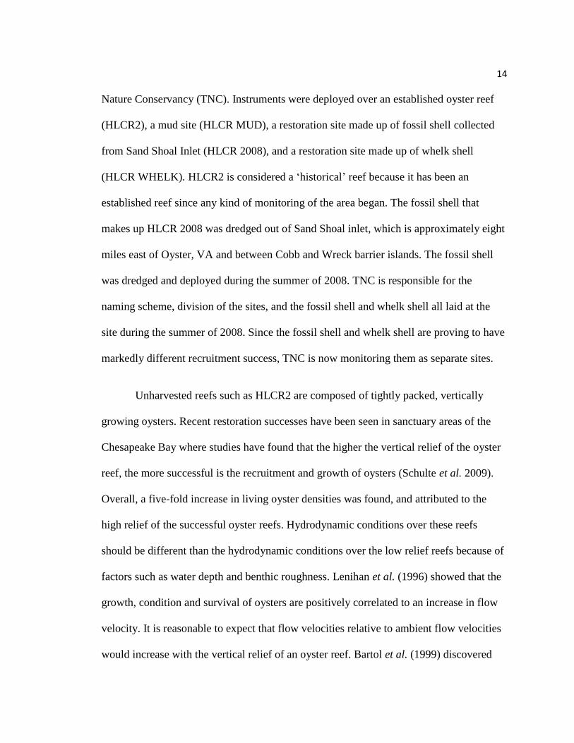
Nature Conservancy (TNC). Instruments were deployed over an established oyster reef

(HLCR2), a mud site (HLCR MUD), a restoration site made up of fossil shell collected

from Sand Shoal Inlet (HLCR 2008), and a restoration site made up of whelk shell

(HLCR WHELK). HLCR2 is considered a ‗historical‘ reef because it has been an

established reef since any kind of monitoring of the area began. The fossil shell that

makes up HLCR 2008 was dredged out of Sand Shoal inlet, which is approximately eight

miles east of Oyster, VA and between Cobb and Wreck barrier islands. The fossil shell

was dredged and deployed during the summer of 2008. TNC is responsible for the

naming scheme, division of the sites, and the fossil shell and whelk shell all laid at the

site during the summer of 2008. Since the fossil shell and whelk shell are proving to have

markedly different recruitment success, TNC is now monitoring them as separate sites.

Unharvested reefs such as HLCR2 are composed of tightly packed, vertically

growing oysters. Recent restoration successes have been seen in sanctuary areas of the

Chesapeake Bay where studies have found that the higher the vertical relief of the oyster

reef, the more successful is the recruitment and growth of oysters (Schulte et al. 2009).

Overall, a five-fold increase in living oyster densities was found, and attributed to the

high relief of the successful oyster reefs. Hydrodynamic conditions over these reefs

should be different than the hydrodynamic conditions over the low relief reefs because of

factors such as water depth and benthic roughness. Lenihan et al. (1996) showed that the

growth, condition and survival of oysters are positively correlated to an increase in flow

velocity. It is reasonable to expect that flow velocities relative to ambient flow velocities

would increase with the vertical relief of an oyster reef. Bartol et al. (1999) discovered

15

that mid-intertidal oysters within reef interstices grow faster and live longer than oysters

at the reef surface, and suggested that factors such as hydrodynamics vary between

locations along the reef.

Figure 2.1: (A) Areal view of Hillcrest reef tract, the location of the Anheuser Busch Coastal

Research Center and the location of the study site; (B) Specific deployment locations in relation to the

channel as outlined by The Nature Conservancy

2.2.2 Elevation and roughness measurements

To define the elevation and benthic roughness, all sites were first surveyed to

obtain relative elevations every 20 cm along multiple transects. A LaserMark LM800

Rotary Laser, with an accuracy of 1/16‖ at 100 ft, was placed on a tripod placed at a

center point on the reef marked by an aluminum stake. HLCR2 was surveyed with 11

16

transects of varying lengths up to 15 m radiating from the center stake. The surveys of

HLCR WHELK (Figure 2.2) and HLCR 2008 consisted of eight 6 m transects, and the

survey of HLCR MUD consisted of four 6 m transects.

Figure 2.2: Top left: Laser Mark LM800 Series rotating laser mounted on a tripod; Bottom left:

Taking elevation measurement with a stadia rod every 20 cm along the transect tape; Right: Location of 6

m transects on HLCR WHELK surveyed for elevation relative to the rotating laser eye mounted on a tripod

in the center

Along each transect, the distance to the laser beam from the reef was measured

every 20 cm using a hand held laser detector and a stadia rod. The 20 cm resolution was

chosen to determine the variability and overall roughness differences between each site.

With the height of the laser eye and distance from the laser to the ground at each stadia

reading known, the relative elevations of each point were determined. The relative

elevations were corrected by adjusting them according to a base point established using a

17

survey grade Trimble R8 GPS system. The Trimble R8 GPS unit has a horizontal

accuracy to within 1 cm and a vertical accuracy from 2-3 cm. The Trimble R8 collected

static observations of broadcasts from regional CORS base stations for approximately

two hours in order to triangulate its exact position. Geoid09 was the model used for

calculating elevation and the observations were processed using OPUS which is a

commonly used method for this kind of GPS. Each data point from the laser lever survey

was then adjusted to UTM NAD83, which is commonly used as a coordinate system and

datum. The Trimble R8 was set at the center stake on HLCR 2008, and all elevations are

relative to this datum unless otherwise specified. The instruments were deployed at the

center origin of the surveyed transects. Elevations at the center point, relative to HLCR2,

are: HLCR2: 0 cm, HLCR MUD: -37.16 cm, HLCR WHELK: -30.81 cm and HLCR

2008: -0.33 cm.

The four sites (Figure 2.1) differ in elevation by less than 40 cm. Sample transects

of each site are illustrated in Figure 2.3. Here the differences in elevation are apparent,

and a visual of the roughness differences at a 20 cm resolution is provided. HLCR MUD

is the site found at the lowest elevation. HLCR 2008 is a mound of fossil shell that drops

off in elevation away from the center. HLCR WHELK has a noticeable depression in the

center where the instrument was placed and elevation increases towards the outside of the

reef where mostly live oysters were observed. HLCR2 is relatively high in elevation at its

crest and gradually decreases towards the surrounding mud flats and the channel. HLCR2

appears to have the greatest variability at the 20 cm resolution.

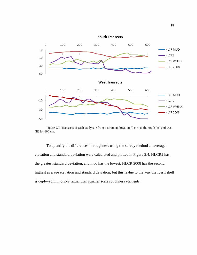
18

Figure 2.3: Transects of each study site from instrument location (0 cm) to the south (A) and west

(B) for 600 cm.

To quantify the differences in roughness using the survey method an average

elevation and standard deviation were calculated and plotted in Figure 2.4. HLCR2 has

the greatest standard deviation, and mud has the lowest. HLCR 2008 has the second

highest average elevation and standard deviation, but this is due to the way the fossil shell

is deployed in mounds rather than smaller scale roughness elements.

19

Figure 2.4: Elevations and topographic variability (standard deviation) relative to the HLCR MUD

measured every 20 cm along 600 cm transects

2.3 Large scale hydrodynamics

2.3.1 Effects of elevation on flow and circulation

Three Nortek Inc.© Aquadopp Profilers (AQDPs) were deployed at three

elevations on HLCR2 (Figure 2.5). The AQDPs have internal memory capacity and thus

can be deployed autonomously for extended periods of time. Two of the AQDPs used in

the elevation study are High Resolution (HR) and capture vertical profiles of the 3-

dimensional velocities and mean flow patterns throughout the entire water column. The

AQDPs capture velocities and mean flow patterns at a vertical resolution of 3 cm, a

sampling rate of 32 Hz, and a horizontal velocity range of 30 cm s-1

(all adjustable

20

parameters). One other AQDP used was not a HR profiler, and collected velocities at a

vertical resolution of 10 cm. The AQDPs were secured on frames constructed to sit on the

seafloor and adjusted to minimize the tilt and role of the instrument.

The first AQDP (HR) was placed on the crest of the reef (HLCR_H) 75 cm above

the mud floor, the second (HR) was placed midway up the reef (HLCR_M) 35 cm above

the mud floor, and the third (not HR) was placed on the mud floor (HLCR_L) at the base

of the reef. Oyster density and bed roughness was visually observed to be highest at

OYST_H, moderate at OYST_M, and lowest at OYST_L. The three instruments were

positioned along a line perpendicular to the main axis of the channel at a spacing of 3.65

m between instruments (Figure 2.5). Velocity profiles using the Vectrino were also taken

adjacent to each of the AQDPs to profile the flow at a greater resolution and at a closer

proximity to the substrate.

Figure 2.5: The three Aquadopps deployed for the Elevation Study were measured to be 365 cm

from sensor to sensor. The elevation difference from OYST_L to OYST_M was 35.7 cm and from

OYST_M to OYST_H was 39.5 cm.

21

The AQDPs at OYST_H and OYST_M were both HRs. They were set to sample

continuously at a rate of 1 Hz and 3 cm bin resolution. The third AQDP at the base of the

reef was on loan from Dr. Pat Wiberg and was not an HR and had less storage memory

than the other two AQDPs deployed. The low resolution AQDP was deployed at the

location with the deepest water column, OYST_L, where it could collect data from the

greatest number of bins. The bins were set to the highest possible resolution, 10 cm, and

the instrument collected data at a rate of 1 Hz for the maximum amount of time allowed

given the limited memory. The start of data collection for this instrument was delayed by

one half of a tidal cycle so that all three AQDPs were collecting data while micro-

profiling of the flow adjacent to the reef was done using the Vectrino.

For the elevation experiment conducted on HLCR2, measurements were taken

along a transect of increasing elevation across the reef. One difference between this study

and those discussed above is the difference in tidal range. The previous studies by

Lenihan et al (1996, 1999) and Schulte et al. (2009) were done along the dominant

upstream-downstream flow direction in an estuary with a tidal range of only ~20 cm. The

data collected during this experiment were taken across a transect perpendicular to the

predominant direction of flow, during all tidal stages, with a tidal range of 1-2 m (Figure

2.6). Because of this difference and the asymmetric tides experienced in this area,

velocity measurements were taken over five consecutive tidal cycles.

The instrument at OYST_L never comes completely out of water, whereas, the

instruments at OYST_M and OYST_H do come out of water or are in water too shallow

for data collection around low tides. For the purposes of comparison between sites, only

22

data collected when all instruments are collecting is considered. The AQDP at OYST_L

were set to start data recording one tidal cycle later than the others because of its limited

memory capacity. Water depth at OYST_L nearly reached 2 m, whereas depths at

OYST_M and OYST_H did not rise above 1.5 m. The depths recorded at OYST_H are

all slightly high due to the water being too shallow for the sensors to work properly. The

depths used in calculations were adjusted based on observations taken while the

instruments were deployed.

Figure 2.6: Mean depth as recorded by the three AQDPs simultaneously at the threeelevations

over a period of three days.

23

Velocities were compared during different tidal stages such as flooding, ebbing,

peak, and slack. A depth of 35 cm above the bed was analyzed across time for all

AQDPs. This depth was chosen to allow for the blanking distance of the instruments and

because it is a water column depth achieved at all sites for a decent amount of time across

the tidal cycles. By doing this, differences in flow speeds can be analyzed independent of

differing water column influences. Data collected by the AQDPs was processed to obtain

vertical velocity profiles for the Up, North and East directions (See Appendix II), depth

averaged velocity, and the horizontally averaged velocity. From the velocity data, shear

velocity, u*, and roughness length-scale, z0, were calculated, using the ―Law of the Wall‖

equation:

, (2.1)

where ĸ=0.41 is Von Karman‘s constant and d is the predetermined roughness height

which is a vertical off-set to account for changes in elevation of the bed relative to datum.

Because the flow in the benthic boundary layer is assumed to be turbulent and fully

rough, the law of the wall can be used to appropriately describe the velocity profile

(Cheng et al. 1999).

Due to surface reflections of the acoustic pulses in shallow waters, velocity

records for the AQDPs are corrupted near the water surface and result in acceptable data

collected for only the bottom one half of the water column over OYST_H. This surface

reflection also accounts for the band of zero velocity in the third tidal cycle of OYST_H.

Around day 182 during one tidal signal the AQDPs measured throughout the water

24

column. This was likely due to an extremely calm day and therefore the instrument

recorded more accurate data closer to the surface.

High flow is observed at low and mid elevations before the water is deep enough

to get data at the crest of the reef (Figures 2.7 and Appendix II).

Figure 2.7: Horizontally averaged velocities over 5 consecutive tidal cycles taken simultaneously

at 3 elevations

Horizontally averaged velocity magnitude (U) was calculated as the root mean

square of the east and north velocities:

(2.2)

25

where Ue is east velocity, Un is the north velocity, and U is the velocity magnitude

(Figure 2.7). Depth averaged mean U for OYST_L, OYST_M, and OYST_H are 17.34,

7.68, and 2.75 cm/s respectively (Table 2.1). The drastic differences in depth averaged U

between elevations appearing within color plots for OYST_M and OYST_H may be

misleading, because feather plots show that the magnitude of velocity at an elevation of

20 cm is not drastically different between elevations (Figure 2.8).

Figure 2.8: Feather plots of U at 20 cm above the substrate over five consecutive tidal cycles taken

simultaneously at the three elevations

While the majority of the results can be attributed to local conditions (e.g. bed

roughness at the point of measurement), some are linked to circulation patterns created by

26

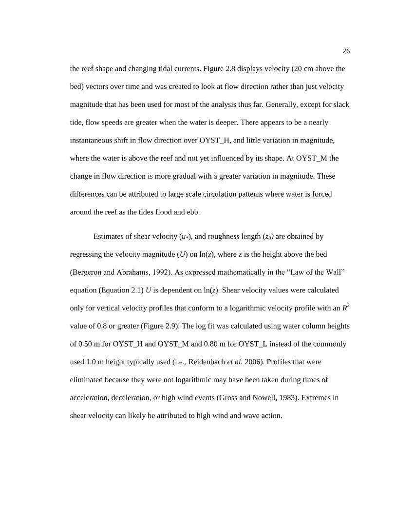
the reef shape and changing tidal currents. Figure 2.8 displays velocity (20 cm above the

bed) vectors over time and was created to look at flow direction rather than just velocity

magnitude that has been used for most of the analysis thus far. Generally, except for slack

tide, flow speeds are greater when the water is deeper. There appears to be a nearly

instantaneous shift in flow direction over OYST_H, and little variation in magnitude,

where the water is above the reef and not yet influenced by its shape. At OYST_M the

change in flow direction is more gradual with a greater variation in magnitude. These

differences can be attributed to large scale circulation patterns where water is forced

around the reef as the tides flood and ebb.

Estimates of shear velocity (u*), and roughness length (z0) are obtained by

regressing the velocity magnitude (U) on ln(z), where z is the height above the bed

(Bergeron and Abrahams, 1992). As expressed mathematically in the ―Law of the Wall‖

equation (Equation 2.1) U is dependent on ln(z). Shear velocity values were calculated

only for vertical velocity profiles that conform to a logarithmic velocity profile with an R2

value of 0.8 or greater (Figure 2.9). The log fit was calculated using water column heights

of 0.50 m for OYST_H and OYST_M and 0.80 m for OYST_L instead of the commonly

used 1.0 m height typically used (i.e., Reidenbach et al. 2006). Profiles that were

eliminated because they were not logarithmic may have been taken during times of

acceleration, deceleration, or high wind events (Gross and Nowell, 1983). Extremes in

shear velocity can likely be attributed to high wind and wave action.

27

Figure 2.9: Depth plotted u* at 35 cm above the substrate

Shear velocity, as well as U, at all elevations is greatest on either side of slack

tide. The shallow water conditions and lack of a well defined boundary layer flow at

OYST_H made the fitting of a log profile to the velocity data difficult. The AQDP at

OYST_L was not a high resolution instrument, and therefore had fewer points to fit to the

log profile. At OYST_M, however, the instrument was a high resolution AQDP in less

shallow water. Here, a good number of vertical velocity profiles conformed to the

logarithmic velocity profile, and thus it was reasonable to calculate a greater number of

28

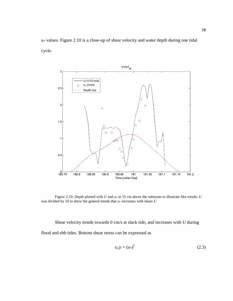
u* values. Figure 2.10 is a close-up of shear velocity and water depth during one tidal

cycle.

Figure 2.10: Depth plotted with U and u* at 35 cm above the substrate to illustrate like trends; U

was divided by 10 to show the general trends that u* increases with mean U

Shear velocity trends towards 0 cm/s at slack tide, and increases with U during

flood and ebb tides. Bottom shear stress can be expressed as

τb/ρ = (u*)2 (2.3)

29

and is directly responsible for vertical mixing and sediment suspension and deposition

(Cheng et al. 1999). For comparison between elevations mean and median u* and z0 are

displayed in Table 2.1. Mean u* for the entire measurement period is greatest, 2.37 cm/s,

at OYST_L, lowest, 1.16 cm/s, at OYST_M and also relatively low, 1.47 cm/s, at

OYST_H, so it is expected that sediment motion is greatest at the lowest elevation. The

relatively greater u* values correspond with greater velocities at OYST_L.

Location Elevation

(cm) Ud

(cm/s) u* Mean (cm/s)

z0 Mean (cm) CD

OYST_H 76.2 11.36 1.47 0.96 0.015

OYST_M 40.0 13.42 1.16 0.30 0.0098

OYST_L 0.0 18.35 2.37 0.61 0.0088

Table 2.1: Calculation parameters and drag coefficients calculated using Equations 2.1 and 2.4 and

a height from the bottom of 0.35 for OYST_H and OYST_M and 0.40 for OYST_L. Ud is the depth

averaged velocity. Elevations are relative to the mud flat at OYST_L.

To quantify the drag experienced on the water flow by the benthic roughness at

each location, a drag coefficient (CD) was calculated to quantify roughness at each

location (Reidenbach et al., 2006):

(2.4)

where U0 is the instantaneous horizontally averaged velocity at an elevation of z = 40 cm

above the bed. In agreement with visual observations (Figure 2.11), CD increased with

elevation: 0.0088 at OYST_L; 0.0098 at OYST_M; and 0.015 at OYST_H. The apparent

trends of u* decreasing with elevation and CD increasing with elevation are opposite since

30

water velocity decreases near high tide and CD is calculated directly from u*. A

displacement height (d0) corrected for instrument placement relative to the surrounding

vertical oysters at the highest elevation. At the lower two elevations live oysters were

fewer and did not protrude into the water column above the instrument head. Peak drag

occurs over the top of the reef with CD=0.015. This is approximately 5 times greater than

the canonical value of CD=0.003 often reported for flows over muddy sites (i.e., Gross

and Nowell, 1983). The drag coefficients are comparable to those found by Reidenbach

et al. (2006) over a fringing coral reef.

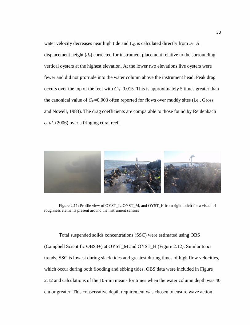
Figure 2.11: Profile view of OYST_L, OYST_M, and OYST_H from right to left for a visual of

roughness elements present around the instrument sensors

Total suspended solids concentrations (SSC) were estimated using OBS

(Campbell Scientific OBS3+) at OYST_M and OYST_H (Figure 2.12). Similar to u*

trends, SSC is lowest during slack tides and greatest during times of high flow velocities,

which occur during both flooding and ebbing tides. OBS data were included in Figure

2.12 and calculations of the 10-min means for times when the water column depth was 40

cm or greater. This conservative depth requirement was chosen to ensure wave action

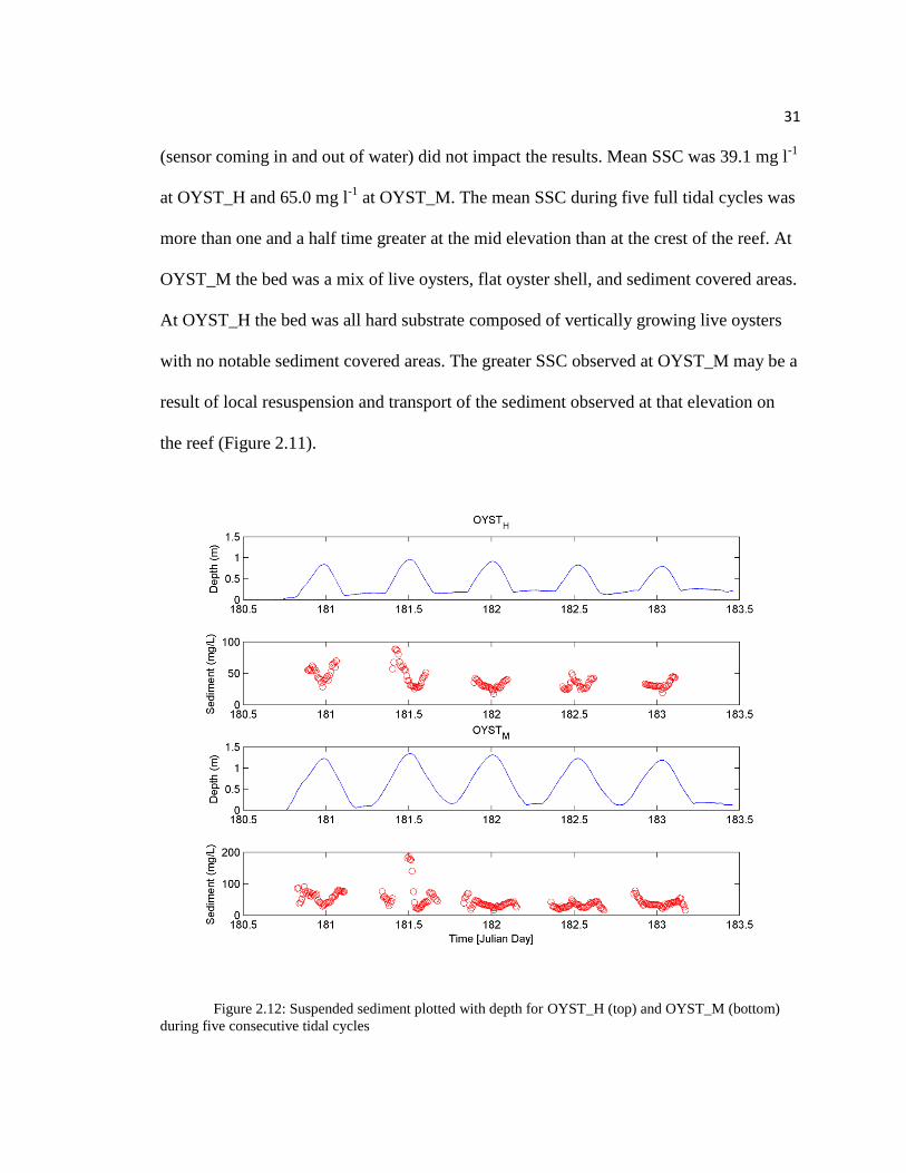
31

(sensor coming in and out of water) did not impact the results. Mean SSC was 39.1 mg l-1

at OYST_H and 65.0 mg l-1

at OYST_M. The mean SSC during five full tidal cycles was

more than one and a half time greater at the mid elevation than at the crest of the reef. At

OYST_M the bed was a mix of live oysters, flat oyster shell, and sediment covered areas.

At OYST_H the bed was all hard substrate composed of vertically growing live oysters

with no notable sediment covered areas. The greater SSC observed at OYST_M may be a

result of local resuspension and transport of the sediment observed at that elevation on

the reef (Figure 2.11).

Figure 2.12: Suspended sediment plotted with depth for OYST_H (top) and OYST_M (bottom)

during five consecutive tidal cycles

32

2.3.2 Hydrodynamics of various bed substrates: Multi-site study

With restoration efforts using different substrates (Figure 2.13) currently

underway in the Hillcrest oyster track (Figure 2.1), where the study site is located, a

comparison study of hydrodynamics over the different substrates was conducted to

provide insight into how substrate impacts the varying success of restoration methods.

Figure 2.13: From left to right: HLCR MUD--mud, HLCR 2008--fossil oyster shell, HLCR

WHELK--whelk shell, HLCR2--live oysters

A visual survey of the restoration sites, HLCR 2008 and HLCR WHELK, reveals

many more living adult oysters growing on the whelk shell than on the fossil oyster shell

(Also see Table 3.3 in the Recruitment study results).

For the multi-site study, four AQDP s were deployed at four different sites, all

adjacent to one another, to measure velocity and mean flow patterns. The site names will

be used to identify the AQDP deployments during this study. The first AQDP was placed

on the historical (healthy) reef, HLCR2, the second was placed on HLCR WHELK, the

third was placed on a mound of fossil shell within HLCR 2008 which, and the fourth

AQDP was placed at HLCR MUD to get a bulk flow baseline (Figure 2.14). All AQDPs

33

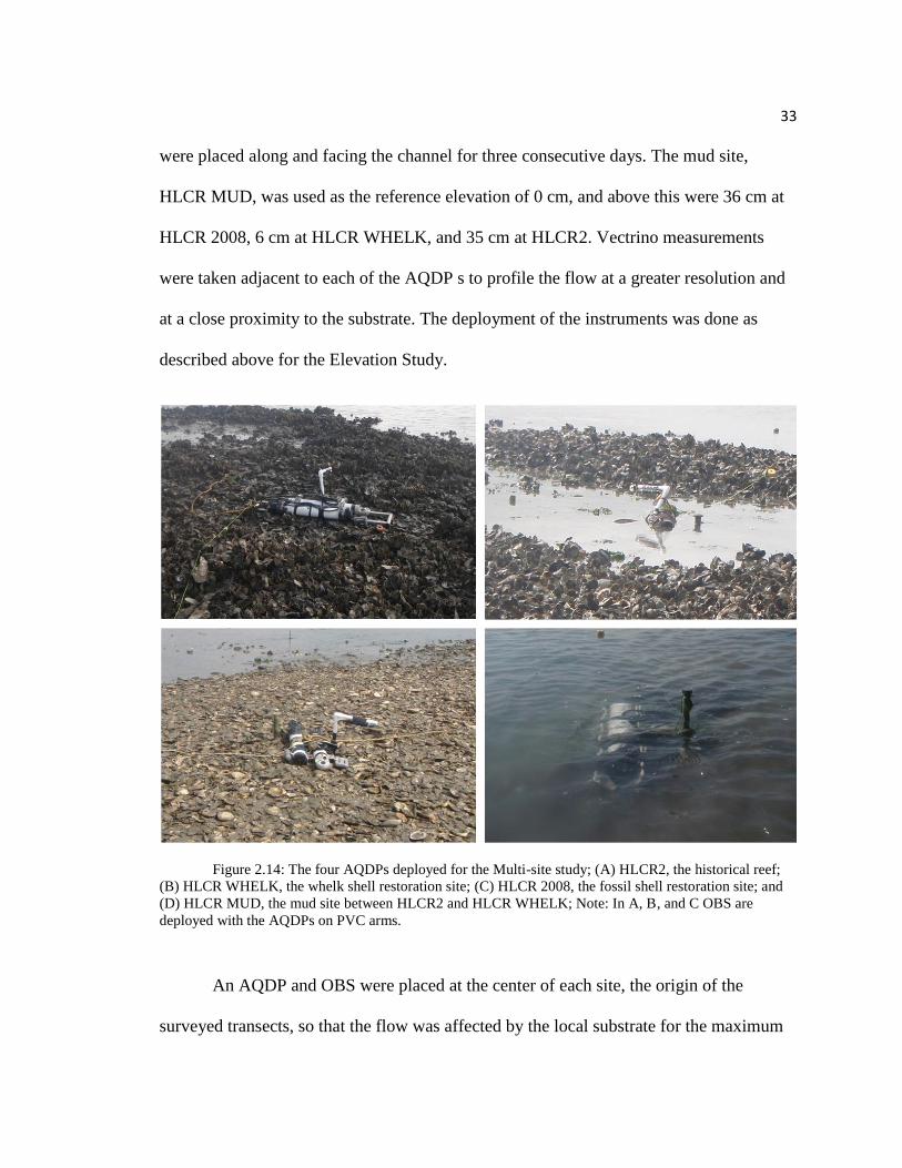
were placed along and facing the channel for three consecutive days. The mud site,

HLCR MUD, was used as the reference elevation of 0 cm, and above this were 36 cm at

HLCR 2008, 6 cm at HLCR WHELK, and 35 cm at HLCR2. Vectrino measurements

were taken adjacent to each of the AQDP s to profile the flow at a greater resolution and

at a close proximity to the substrate. The deployment of the instruments was done as

described above for the Elevation Study.

Figure 2.14: The four AQDPs deployed for the Multi-site study; (A) HLCR2, the historical reef;

(B) HLCR WHELK, the whelk shell restoration site; (C) HLCR 2008, the fossil shell restoration site; and

(D) HLCR MUD, the mud site between HLCR2 and HLCR WHELK; Note: In A, B, and C OBS are

deployed with the AQDPs on PVC arms.

An AQDP and OBS were placed at the center of each site, the origin of the

surveyed transects, so that the flow was affected by the local substrate for the maximum

34

distance considering the changing flow direction with the tides. The general tidal trends

seen in the Elevation Study are the same for this study as well. The bulk flow results

shown in Figure 2.15 are very similar to Figure 2.7.

The instruments, and surrounding substrate, were submerged for the greatest

amount of time at the HLCR MUD because of it‘s relatively low elevation and was

submerged for the least amount of time at HLCR2. The depths recorded at HLCR2 are all

slightly high due to the water being too shallow for the sensors to work properly. Depths

used in calculations were adjusted based on observations taken while the instruments

were deployed.

Data was collected with the AQDPs in East-North-Up (ENU) coordinates, with

dominant flow along the Northeast/Southwest direction parallel to the channel. Due to

surface reflections of the acoustic pulses in shallow waters, velocity records are corrupted

near the water surface and result in acceptable data collected for only the bottom one half

of the water column over HLCR2 and HLCR 2008. Extremely calm surface conditions

likely account for the times where it appears that the AQDP measure throughout the

water column, such as in the fifth tidal cycle.

Flow velocities at all sites increase with depth during most tidal cycles and at all

sights velocity drops to 0 cm/s at slack tide (Figures 2.15 and Appendix II). The

instruments on HLCR WHELK and HLCR MUD were located at lower elevations than

HLCR 2008 and HLCR2. The higher elevations experienced maximum velocity directly

on either side of slack tide and typically for a time period less than 60 minutes. At the

35

two lower elevations, mean velocities near 20 cm/s were observed for several hours on

either side of slack tide.

Figure 2.15: Horizontally averaged velocities over five consecutive tidal cycles taken

simultaneously at the four sites

The depth averaged mean velocities (Ud) were recorded at HLCR2 and HLCR

WHELK and were three and four times greater than those at HLCR 2008 and HLCR

MUD. The mud site is located between HLCR WHELK and HLCR2, and the vertical

relief of the adjacent reefs may be creating this low velocity zone over the lower

elevation mud site. Having these low flow zones between reefs could be beneficial if

sediment and resuspended pseudo-feces from adjacent reefs settles there instead of being

carried onto reefs further downstream. Feather plots (Figure 2.16) show that the

magnitude of velocity at an elevation of 20 cm is not drastically different between sites.

36

Figure 2.16: Feather plots of U at 20 cm above the substrate over five consecutive tidal cycles

taken simultaneously at the four sites

The feather plots indicate mean flow parallel to the channel and reversing

direction with tidal changes at all sites. At HLCR MUD, which is the last site to drain at

low tide, the flow direction is toward the channel just before the AQDP comes out of

water. This happens because this site is between HLCR WHELK and HLCR2 which

block flow parallel to the channel from HLCR MUD below their elevations (Figure 2.1).

37

Location

Elevation

(cm)

U d

(cm s-1)

u *

(cm s-1)

z 0

(cm) C D

HLCR2 37.2 11.7 1.23 0.28 0.015

HLCR WHELK 6.4 15.6 1.84 0.74 0.014

HLCR 2008 36.8 11.0 0.65 0.11 0.0026

HLCR MUD 0.0 18.5 1.72 0.33 0.0044

Table 2.2: Calculation parameters and drag coefficients calculated using Equations 2.1 and 2.4 and

a height from the bottom of 0.35 for HLCR2, HLCR WHELK and HLCR 2008 and 0.40 for HLCR MUD.

Ud is the depth averaged velocity, and elevations are relative to HLCR MUD.

CD (Equation 2.4) for the various sites followed expectations with greatest

magnitudes at HLCR2 and lowest at HLCR 2008. The vertical relief and high roughness

of HLCR2 produced a relatively high u* and caused Ud to be relatively low. At HLCR

2008 the vertical relief was also relatively high, so the shallow water conditions over the

AQDP caused a low Ud. However, the lack of local roughness elements leads to a low u*

value. The drag coefficients are comparable to those found in the Elevation study

discussed above and by Reidenbach et al. (2006) over a fringing coral reef.

38

Figure 2.17: Depth and u* plotted at 35 cm above the substrate over six consecutive tidal cycles

As observed in the Elevation study, the trend of increasing u* with velocity

recorded shortly before and after slack tide as the flow is decelerating and accelerating is

also seen here. Depicted in Figure 2.17, u* neared 0 cm/s during slack tides at HLCR2,

HLCR WHELK, and HLCR 2008. However, at HLCR MUD the velocity profiles did not

meet the requirement of having an R2 value of 0.80 or greater at times of low flow so u*

was not calculated. This helps to explain why the mean u* at HLCR MUD was greater

than at HLCR2 and HLCR 2008.

39

Figure 2.18: Suspended sediment concentration plotted at HLCR2 across six consecutive tidal

cycles at times when water depth was greater than 20 cm

The OBSs were positioned 17 cm above the substrate at each site and the data was

filtered to only include values when the water was greater than 40 cm deep (Figures 2.18-

2.20). Similar trends to u* are seen with relatively high concentrations observed shortly

before and after slack tide, aligning with high flow velocities. However, differing from

u*, SSC increases during flood tides, but a mirrored decrease in SSC during ebb tides in

not observed.

40

Figure 2.19: Suspended sediment concentration at HLCR WHELK plotted across six consecutive

tidal cycles at times when water depth was greater than 40 cm

To compare SSC between sites, a mean sediment concentration value over the

length of data collection period was calculated. Mean SSC was 53.2 mg l-1

at HLCR2,

62.7 mg l-1

at HLCR WHELK, and 64.3 mg l-1

at HLCR 2008 indicating that the bed of

live oysters exhibited a decrease in sediment concentration. These results suggest that

live oysters comprising a local area of hard substrate may contribute to the decrease in

SSC due to their contribution to hard-substrate roughness and their active filtering (for

preliminary sediment flux results refer to appendix I).

41

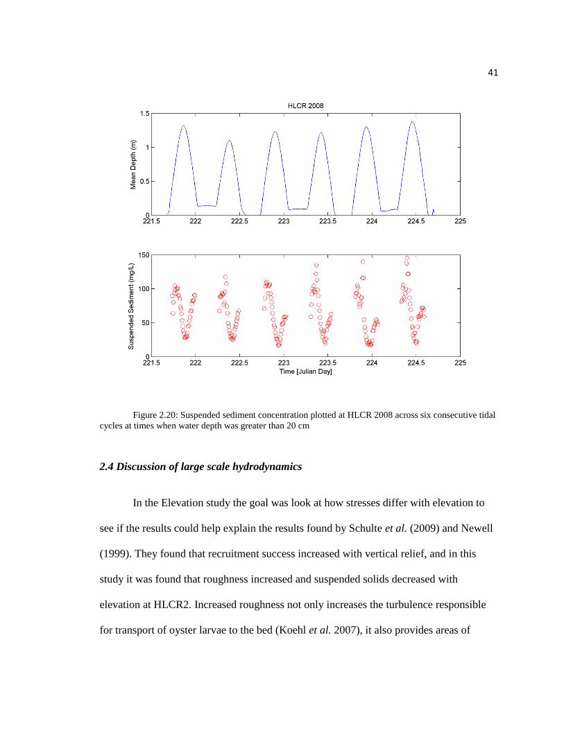
Figure 2.20: Suspended sediment concentration plotted at HLCR 2008 across six consecutive tidal

cycles at times when water depth was greater than 20 cm

2.4 Discussion of large scale hydrodynamics

In the Elevation study the goal was look at how stresses differ with elevation to

see if the results could help explain the results found by Schulte et al. (2009) and Newell

(1999). They found that recruitment success increased with vertical relief, and in this

study it was found that roughness increased and suspended solids decreased with

elevation at HLCR2. Increased roughness not only increases the turbulence responsible

for transport of oyster larvae to the bed (Koehl et al. 2007), it also provides areas of

42

refuge from predators (Soniat et al. 2004) and shear stress that could dislodge a larva

before it attaches (Reidenbach et al. 2009).

In the Multi-site study the effects of bed roughness on the distribution of sheer

stress were investigated by taking small scale velocity measurements over four sites

adjacent to one another: a living reef, a whelk shell restoration reef, a fossil oyster shell

restoration reef and a mud site. Large-scale velocities were measured over the same four

sites to compare to the large scale flow patterns. Mean velocities decreased with

elevation, while shear velocity appeared to be affected by the vertical relief of the site as

well as local roughness. The drag coefficient did support the observation that HLCR2 and

HLCR WHELK had greater roughness than HLCR 2008 and HLCR MUD. As in the

Elevation study, mean suspended solids increased with observed roughness of the sites.

These results suggest that beds with greater elevation and roughness provide a

better habitat for larval recruitment and growth than beds with lower elevation and

roughness. In terms of the current restoration efforts being conducted by TNC, the whelk

shell bed is a more suitable habitat for larval recruitment and growth than the fossil oyster

shell bed.

43

Chapter 3

Structure Manipulation Study: Flume and Field

3.1 Motivation

Oyster larvae, like many other bivalve larvae, determine proper settlement sites

depending upon local hydrodynamics (Koehl and Hadfield 2010). At the scale of oyster

larvae, turbulence and fluid shear dictate hydrodynamic forces on larvae which have

settled onto benthic surfaces. It has been observed in laboratory studies (Crimaldi et al.

2002, Koehl and Hadfield 2004) that certain hydrological conditions are ideal for larval

settlement. Larvae preferentially settle where turbulent advection transports them to

within the benthic boundary layer, on surfaces where shear stress is high, but once

settled, where they have enough refuge from stresses to cement themselves to the

substrate (such as in microhabitats or during lulls in near-bed turbulent stresses)

(Crimaldi et al. 2002, Soniat 2004). Coupled with the benthic roughness of a living reef,

larval transport to the bed is facilitated by turbulent mixing (Hendriks et al. 2006). The

turbulence created by the morphology of an oyster reef not only brings food, such as

phytoplankton, closer to the adult oysters but also transports oyster larvae to new

settlment sites (Lenihan 1999). The turbulence transports the larvae to the bed, bringing

them in contact with the benthos multiple times so that if they find their first landing site

to be unsuitable they can release themselves back into the flow and test the next site they

come in contact with (Fuchs et al. 2007; Soniat 2004).

44

In studies determining the impact of flow on oyster and barnacle larvae,

settlement has been found to increase with velocity and shear (Bushek 1988; Soniat

2004), and barnacle larvae select local micro-sites with low shear (Wethy 1986). This

low shear is often associated with crevices and narrow protective burrows that could be

provided between roughness elements. Aimed at furthering this work, my study was

designed to test how the position within a reef affects the instantaneous hydrodynamic

forces experienced by C. virginica larva along settlement substrate of different geometric

roughness.

To investigate these hydrodynamic forces, simplified structures of repeating and

vertically oriented roughness elements were constructed and positioned within a

laboratory flume. This study included flume studies of flow over 10 different benthic

structures ranging from a flat bed to an idealized topography similar to that of an oyster

reef. Five different bulk flow speeds were tested for each roughness, and a field study of

recruitment on five replicates of three structure manipulations was also performed to

determine how benthic roughness impacts recruitment success. Combined, both lab and

field studies were used to determine the effects of benthic roughness on shear stresses and

larval settlement.


3.2.1 Field Materials and Methods

Traditionally used in hydraulic laboratories, a Vectrino (Acoustic Doppler

Velocimeter) was taken into the field to measure fine scale hydrodynamics between

45

tightly spaced live oysters in situ. The Vectrino was mounted on a stainless steel frame on

an adjustable arm so that it could be raised and lowered to sample at the desired

elevation. The Vectrino does not have internal memory storage capability, therefore data

is transferred using a 30 m cable to a computer located on a boat moored just offshore of

the reef. Velocity data was collected at 50 Hz for 10,000 samples at each elevation before

the height of the instrument was adjusted. Velocity was measured at approximately 0.5,

1, 2, 3, 4, 5, 7, 10, and then 15 cm above the bed for each vertical transect (Figure 3.1).

This measurement distribution was used so that there was greater resolution close to the

bed where the small scale hydrodynamics and thus larvae are most affected by the

roughness of the bed. The sampling volume for the Vectrino is defined by the intersection

of the beams and is approximately 50 mm from the transmitter. For all profiles taken

during the experiments, the sampling area was set to be 4 mm in diameter (user

selectable) and 6 mm wide (fixed diameter) so that velocity data could be obtained

extremely close to the substrate.

46

Figure 3.1: (A) The Vectrino recording point velocity measurements adjacent to an Aquadopp

(underwater in the background); Inset: The Vectrino probe underwater and above oyster shell; (B) Each

point represents the location where velocity data was collected (0.05, 1, 2, 3, 4, 5, 7, 10, and 15 cm above

the substrate) using the Vectrino, and each column represents on vertical profile.

Velocity measurements were taken with the Vectrino over multiple vertical

transects at randomized locations over the reef and restoration siteVectrino data was

collected for 33 profiles over HLCR2 and five profiles over HLCR 2008. Data over the

historical reef, HLCR2, was collected to determine the variability and distribution of

shear stresses across an unharvested oyster reef. The data for the five profiles over the

fossil shell site was taken to see what hydrodynamics are created over the same substrate

with little or no vertical orientation. To maintain consistency between profiles taken over

each site, all profiles included in the analysis have velocity measurements at an elevation

of ~15 cm +/- 3 cm, and at an elevation <= 2 cm. All data above the point nearest to 15

cm was discarded to exclude wind affects near the surface. Concurrent with Vectrino

47

measurements, bulk flow was also measured using an AQDP placed on the crest of the

reef and within ~1 m of where Vectrino measurements were taken.

Shear velocity, u*, and roughness length-scale, z0, were calculated from the

Vectrino ADV profiles using the ―Law of the Wall‖ (Equation 2.1) and Reynolds stresses

were computed as the time average of the horizontal, u‘, and vertical, w‘, velocity

fluctuations

Reynolds stress =

u'w' (3.1)

The R2 values for each profile were calculated to determine the goodness of fit to

a logarithmic profile. The averages and standard deviations of points along the Reynolds

stress and velocity profiles were calculated and plotted for further analysis and

comparison of HLCR2 to HLCR 2008 hydrodynamics. Sample profiles (Figure 3.2) show

peak Reynolds stresses ~2 cm above the bed at HLCR 2008 and ~6 cm above the bed at

HLCR2. This implies that net momentum transfer, determined by velocity fluctuations, is

greatest near the substrate at HLCR 2008 and over the tips of the oysters at HLCR2.

Within the structure at HLCR2 Reynolds stress sharply decreases indicating an area

sheltered from hydrodynamic stresses.

Displacement heights (d0) were determined based on the mean elevation observed

for all plotted profiles within each site where the profile started to assume a logarithmic

fit. For the restoration site d0 = 0 cm was used and for the healthy reef d0 = 2 cm. To

determine the closeness of fit to a logarithmic profile R2 values were calculated using

data at all elevations above the specified d0. Profiles that did not fit a logarithmic profile

48

with an R2 value of 0.80 or greater were discarded. Any profiles that did not conform to

these parameters were not included in the comparison analysis.

3.2.2 Field velocity profile results

At the restoration site (Table 3.1), HLCR 2008, u* values ranged from 0.47 cm s-1

to 3.37 cm s-1

with a mean of 2.05 cm s-1

, a standard deviation of 1.31 cm s-1

, and a

median of 1.93 cm s-1

. The z0 values ranged from 0.11 cm to 0.45 cm with a mean of 0.24

cm, a standard deviation of 0.13 cm, and a median of 0.20 cm. At the healthy reef (Table

2.1), HLCR2, u* values ranged from 0.69 cm s-1

to 4.41 cm s-1

with a mean of 1.90 cm s-

1, a standard deviation of 1.05 cm s

-1, and a median of 1.78 cm s

-1. The z0 values ranged

from 0.00 cm to 1.66 cm with a mean of 0.35 cm, a standard deviation of 0.50, and a

median of 0.09 cm. Reynolds stresses were also normalized using the equation:

R u'w'

U 2 (3.2)

where the time average of the horizontal, u’, and vertical, w’, velocity fluctuations are

divided by square of the mean velocity magnitude, U, at the top (elevation of ~15 cm) of

each respective profile (Table 3.1).

49

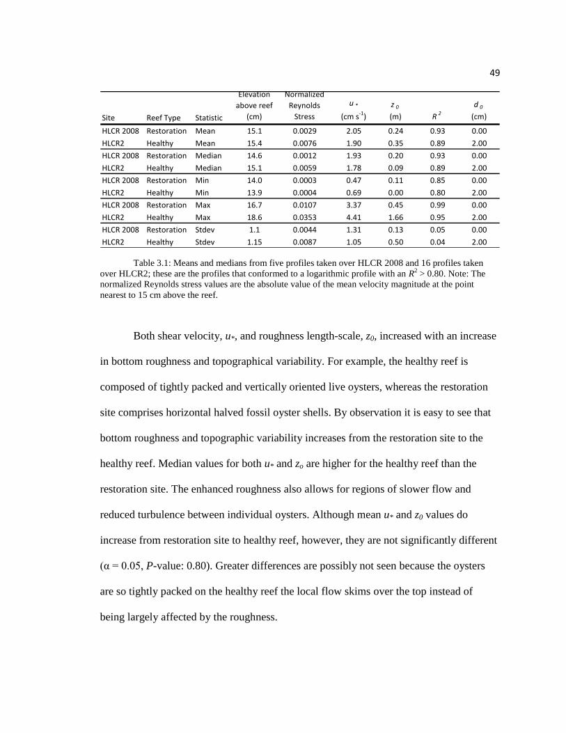
Site Reef Type Statistic

Elevation

above reef

(cm)

Normalized

Reynolds

Stress

u *

(cm s-1)

z 0

(m) R 2

d 0

(cm)

HLCR 2008 Restoration Mean 15.1 0.0029 2.05 0.24 0.93 0.00

HLCR2 Healthy Mean 15.4 0.0076 1.90 0.35 0.89 2.00

HLCR 2008 Restoration Median 14.6 0.0012 1.93 0.20 0.93 0.00

HLCR2 Healthy Median 15.1 0.0059 1.78 0.09 0.89 2.00

HLCR 2008 Restoration Min 14.0 0.0003 0.47 0.11 0.85 0.00

HLCR2 Healthy Min 13.9 0.0004 0.69 0.00 0.80 2.00

HLCR 2008 Restoration Max 16.7 0.0107 3.37 0.45 0.99 0.00

HLCR2 Healthy Max 18.6 0.0353 4.41 1.66 0.95 2.00

HLCR 2008 Restoration Stdev 1.1 0.0044 1.31 0.13 0.05 0.00

HLCR2 Healthy Stdev 1.15 0.0087 1.05 0.50 0.04 2.00

Table 3.1: Means and medians from five profiles taken over HLCR 2008 and 16 profiles taken

over HLCR2; these are the profiles that conformed to a logarithmic profile with an R2 > 0.80. Note: The

normalized Reynolds stress values are the absolute value of the mean velocity magnitude at the point

nearest to 15 cm above the reef.

Both shear velocity, u*, and roughness length-scale, z0, increased with an increase

in bottom roughness and topographical variability. For example, the healthy reef is

composed of tightly packed and vertically oriented live oysters, whereas the restoration

site comprises horizontal halved fossil oyster shells. By observation it is easy to see that

bottom roughness and topographic variability increases from the restoration site to the

healthy reef. Median values for both u* and zo are higher for the healthy reef than the

restoration site. The enhanced roughness also allows for regions of slower flow and

reduced turbulence between individual oysters. Although mean u* and z0 values do

increase from restoration site to healthy reef, however, they are not significantly different

(α = 0.05, P-value: 0.80). Greater differences are possibly not seen because the oysters

are so tightly packed on the healthy reef the local flow skims over the top instead of

being largely affected by the roughness.

50

Representative profiles have been chosen for each study site and a mud bottom

site, HLCR MUD, to further explain and illustrate the hydrodynamics created by the

differences in bottom roughness. The representative velocity profiles are plotted along

with normalized Reynolds stress (Figure 3.2). The Reynolds stress was normalized using

the velocity nearest to 15 cm above the substrate (Eq. 3.2). The Reynolds stress over the

HLCR2 peaked at an elevation of approximately 6 cm, which is the height of the oysters

for this profile and where the velocities begin to assume a logarithmic profile. At HLCR

2008 the Reynolds stress peaks at around 2 cm from the substrate suggesting that there is

less shelter from the hydrodynamic forces such as lift and drag that could prevent settling

of oyster larvae. Reynolds stresses peak at all sites when velocity is 9-11 cm s-1

.

Enhanced roughness creates regions of high turbulence above the bed and lower

turbulence and velocities within the bed structure. At the top of the reef, a strong shear

layer develops within the velocity profile which enhances momentum transport to the

bed. Over HLCR MUD the peak in Reynolds stress is seen at the elevation where an

inversion in the velocity profile occurred. At HLCR 2008 Reynolds stress peaks at -0.006

cm2 s

-2 and is nearly double the peak of -0.0025 cm

2 s

-2 found at HLCR2 and HLCR

MUD. The greater Reynolds stress found adjacent to the substrate at HLCR 2008 means

greater net momentum transfer at the substrate surface that could enhance shear acting on

the larvae and enhance larval dislodgement (Reidenbach et al. 2009).

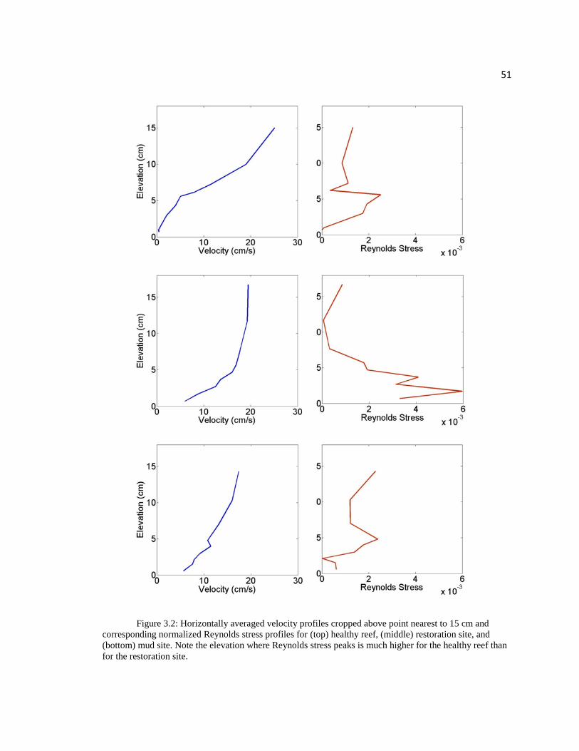
51

Figure 3.2: Horizontally averaged velocity profiles cropped above point nearest to 15 cm and

corresponding normalized Reynolds stress profiles for (top) healthy reef, (middle) restoration site, and

(bottom) mud site. Note the elevation where Reynolds stress peaks is much higher for the healthy reef than

for the restoration site.

52

To further describe how turbulent fluctuations contribute to momentum

distribution throughout the bottom boundary layer (Lu and Willmarth 1973, Luckhik and

Tiederman 1988) quadrant analysis was performed. To perform quadrant analysis, u’ and

w’ velocity fluctuations are divided into four quadrants based on the sign of their

instantaneous values. Contours of the turbulent probability distribution function (pdf) are

shown in Figure 2.5 for turbulence 6 cm above the reef. In quadrant 1 (Q1), u‘ >0, w’ > 0,

in Q2, u’ < 0, w’ > 0 (a turbulent ejection), in Q3, u’ < 0, w’ < 0, and in Q4, u’ > 0, w’ < 0

(a turbulent sweep). Sweeping events, illustrated by pdf values in Q4, transport high

momentum fluid downward towards the reef. Pdf values in Q2 illustrate ejection of low

momentum fluid vertically upwards away from the reef. These ejection and sweep events

result in intermittent flushing of ―dead water‖ that accumulates among roughness

elements (Grass 1971). Growing oysters depend on this flushing to replace seston

depleted water with water containing food. Momentum transport is typically dominated

by these ejection and sweeping events and in this case show up in Q2 and Q4. This is true

for flow over the reef (Figure 3.3), where Reynolds stress factors are dominated by

motions within Q2 and Q4.

53

Figure 3.3: Quadrant analysis of velocity fluctuations located 6 cm above the healthy oyster reef.

The total contribution to the Reynolds Stress within each quadrant was found by

summing the u’w’ contributions: Q1 (8%), Q2 (33%), Q3 (7%), and Q4 (51%). The

combined Q2 and Q4 contributions account for approximately 84% of the total Reynolds

stress, which is similar to results found by other studies of flow over high roughness

topography (Bennet and Best 1996; Lacey and Roy 2008). Q4 events dominate overall;

indicating that the turbulent sweeps of vortices of high energy eddies reaching into the

oyster reef dominate the contribution. For the HLCR 2008, there is a more even balance

of ejection and sweep events (Figure 3.4), with contributions of the quadrants of: Q1

(9%), Q2 (44%), Q3 (10%), and Q4 (37%).

54

Figure 3.4: Quadrant analysis of velocity fluctuations found 6 cm above the restoration reef.

These results suggest that larvae and food carried by high momentum fluid are

swept down to the reef more frequently at HLCR2 than at HLCR 2008. This also

suggests that there is potential for higher rates of larval settlement at HLCR2 simply

because of the higher frequency of larval delivery to the substrate. Growing oysters at

HLCR2 are also provided with food by these sweep events. Even though ejection events

occur more frequently at HLCR 2008 than at HLCR2, flushing still occurs at HLCR2 to

ejection of ―dead water‖ between growing oysters (Grass 1971).

55


3.3.1 Laboratory Materials and Methods

The laboratory-based flume study quantified specific hydrodynamic forces such

as lift, drag, and turbulent bed shear stresses acting along different surfaces adjacent to an

oyster bed that may impact larval settlement. Experiments were conducted within an

open channel recirculating water flume (Figure 3.5), designed based on schematics by

Tamburri et al. (1996). The flume used in the Tamburri et al. (1996) studied dissolved

chemical cues inducing the settlement of Crassostrea virginica larvae (Jonsson et al.

2006) and was therefore considered a useful flume for micro-scale turbulence studies.

The flume was constructed using Lexan ™, a polycarbonate resin thermoplastic, to be 20

cm wide, with 20 cm high walls, with semicircular ends of radius 40 cm and with two

straight sections 100 cm long. One straight section is fitted with a glass pane for photo-

image clarity and the motor and flow generation system are fitted in the opposite straight

section. Two additional, yet thinner sheets of Lexan ™ were placed within each curved

section of the flume parallel to the walls to minimize turbulence and secondary flow

conditions created as the flow moves around the curves. The design for the flow

generation system uses 12 inch LP records mounted to a shaft, perpendicular to the flow,

on a motor with a speed controller. This system uses frictional drag to drive the flow,

rather than propulsion from a propeller, creating the appropriate channel flow velocities

without causing lethal damage to organisms (which may be used in future research)

within the flume. The different mean channel flow conditions were created by adjusting

56

to a range of velocities comparable to velocities observed at the field site (approximately

5-25 cm/s).

Figure 3.5: Recirculating water flume: A) Glass imaging section; B) Motor attached to a speed

controller; C) Rotating long play (LP) vinyl records spaced vertically 1 cm apart to generate flow

To mimic benthic roughness that impacts flow and turbulence, an adjustable

benthic structure was constructed from Plexiglas pieces cut to the width of the flume (20

cm) by eight cm (Figure 3.6). The pieces were hinged together in an accordion style

using piano hinges cut to the length of the Plexiglass pieces. The hinges were attached

using silicon glue and reinforced with duct tape. To prevent reflection of the laser used

for velocity studies, a black multipurpose spray paint was used to coat the entire

structure. As the peak spacing increased the peak heights correspondingly decreased from

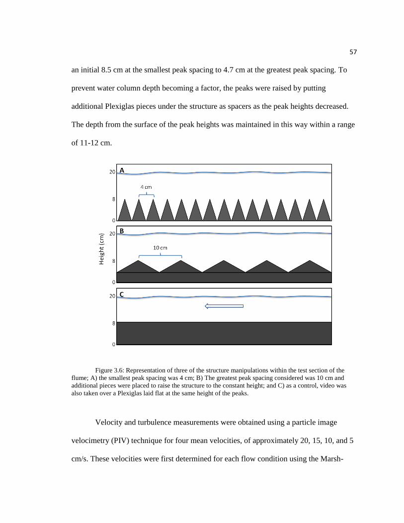
57

an initial 8.5 cm at the smallest peak spacing to 4.7 cm at the greatest peak spacing. To

prevent water column depth becoming a factor, the peaks were raised by putting

additional Plexiglas pieces under the structure as spacers as the peak heights decreased.

The depth from the surface of the peak heights was maintained in this way within a range

of 11-12 cm.

Figure 3.6: Representation of three of the structure manipulations within the test section of the

flume; A) the smallest peak spacing was 4 cm; B) The greatest peak spacing considered was 10 cm and

additional pieces were placed to raise the structure to the constant height; and C) as a control, video was

also taken over a Plexiglas laid flat at the same height of the peaks.

Velocity and turbulence measurements were obtained using a particle image

velocimetry (PIV) technique for four mean velocities, of approximately 20, 15, 10, and 5

cm/s. These velocities were first determined for each flow condition using the Marsh-

58

McBirney flow meter at 4/10th

depth over the adjustable structure and shells and used to

span the range of velocities observed in situ (5-30 cm s-1). Velocity data was collected

over multiple peak heights and spacing and were used to quantify changes in small scale

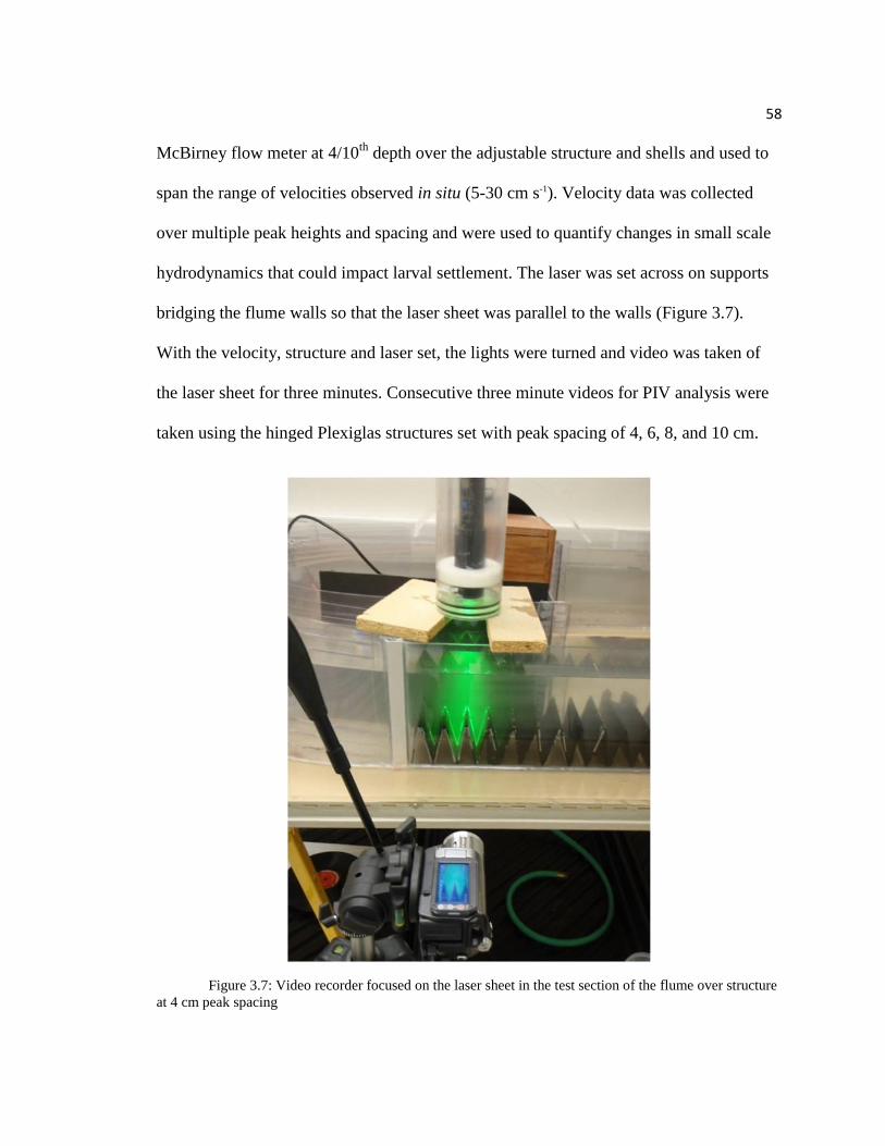
hydrodynamics that could impact larval settlement. The laser was set across on supports

bridging the flume walls so that the laser sheet was parallel to the walls (Figure 3.7).

With the velocity, structure and laser set, the lights were turned and video was taken of

the laser sheet for three minutes. Consecutive three minute videos for PIV analysis were

taken using the hinged Plexiglas structures set with peak spacing of 4, 6, 8, and 10 cm.

Figure 3.7: Video recorder focused on the laser sheet in the test section of the flume over structure

at 4 cm peak spacing

59

The PIV system uses a laser and optics to create a laser light sheet that illuminates

neutrally buoyant particles released into the flow (11 micron silver coated hollow glass

spheres, Potter Industries©). The system consists of the camera, laser, and optics to create

a 10 cm wide by 2 mm thick laser light sheet. The laser is a 30 mW 532 nm green laser

diode and the beam is spread to a sheet using a 30o convex glass lens. Particles are

imaged using a digital video recorder. Videos were separated into 30 images per second

and successive images were processed using Matlab© software that tracks particle

motions over time. PIV was used to view flow in the two-dimensional plane above the

structure within the flume (Figure 3.8).

Figure 3.8: PIV images taken with 4 cm peak spacing and 20 cm s-1

flow velocity; A) Raw image

of particles illuminated by the laser; B) Instantaneous velocity (cm s-1

) color plot created by processing

1,000 successive images using Matlab© software that tracks particle motions over time.

60

The impact of the introduced structure on the mean flow conditions was

determined by taking velocity measurements along vertical transects over the structure

(Figure 3.9), similar to the Vectrino profiles taken over the oyster reef and restoration site

in the field study.

Figure 3.9: Velocity profiles were created from 50 points along a vertical transect above each

structure case. Vertical transects are represented by the yellow lines in color plot of U. There are

recirculation zones within the structure for both the 4 cm and 10 cm cases, but in the 10 cm case the

velocity in the recirculation zone is greater than the velocities in the 4 cm case. Velocity increases

logarithmically with height above the flat surface

61

Point velocities were identified along the surface of the structure to identify areas

within the structure canopy where the small scale hydrodynamics such as drag and shear

stress are suitable for larval settlement. This was done by taking the average of three

point velocities at the surface of the structure surface at ¼, ½, and ¾ depths within the

structure along the surface of the structure for each flow speed/structure manipulation.

The same measurements were also done at the peak of the structure and at the deepest

point within the structure.

3.3.2 Laboratory velocity profile results

Holding bulk flow velocity constant, peak spacing was increased and the velocity

profiles were compared over the flat Plexiglas and for roughness with peak spacings of 4

cm and 10 cm (Figures 3.10-3.13). In all cases the flow profile over the flat Plexiglas

followed the expected logorithmic profile. Within the peak structures velocities remained

low (< 3 cm s-1

), but areas of recirculation were present in all cases. These recirculation

zones, where long lived turbulent eddies are present, are represented by inversions in the

velocity profiles below the depths of the peaks. One area of recirculation reaching flow

speeds of 3-4 cm s-1

was consistently present for all 10 cm peak spacing runs and bulk

flow velocities. However, two areas of recirculation were present for all 4 cm peak

spacing runs at all velocities. Flow speeds reached 2-3 cm s-1

for the recirculation zone

nearest the peaks, but the lower recirculation zones typically had flow speeds of 1 cm s-1

or less.

62

Figure 3.10: Flume velocity 5 cm s-1

and maximum velocity over flat Plexiglas was 8.55 cm s-1



63




Velocity data became unreliable above the structure for flume velocities of 20 cm

s-1

and 25 cm s-1

because the particles were moving too fast to track at 30 images per

second.

64

3.3.3 Instantaneous drag and lift

The vector sum of the instantaneous lift, drag, and time varying acceleration

reaction force (a. r.) are used to describe the instantaneous hydrodynamic forces acting

on oyster larva, which follow the analysis described within Reidenbach et al. (2009). In

unidirectional flow a. r. is minimal (Reidenbach et al. 2009), so the only lift and drag

were needed to describe the hydrodynamic forces in this experiment.

Instantaneous drag (D) including magnitude and direction (parallel to the

direction of water flow):

DpCSuD 25.0 (3.1)

where ρ = 1023 kg m-3

is the density of seawater with salinity = 35 ppt at 25ᵒC, u is the

instantaneous velocity, Sp = 7.07 × 10-8

m2 is the projected area of the 300 µm sphere

(Thompson et al. 1996) normal to the flow direction, and CD = 40 / (u*d/10-6

).

The instantaneous lift force (L) acts normal to the direction of water flow was

calculated by:

L 0.5u2SpCL (3.2)

where Sp = 7.07 × 10-8

m2 is the projected area of the 300 µm sphere normal to the flow

direction, and CL = 0.2 (Wiberg and Smith 1985; Wiberg and Smith 1987).

65

Since the goal of this study was to investigate how hydrodynamics change with

benthic roughness D and L were calculated for structures with spacing between roughness

peaks of 4, 6, 8 and 10 cm. Velocities for calculations were averages of 40 velocity

measurements spanning a ~1.5 cm distance along the surface from PIV estimates.

Velocities used in the analysis were located at the mid-point of elevation between the

peak and trough of the roughness element. Both D and L increase with peak spacing for

all velocities used in this study (Figure 3.14 and Table 3.3). The trend is even stronger

when D and L for all velocities were averaged within each peak spacing. R2 values for D

and L increased to 0.9975 and 0.9822 respectively, but the standard deviations also

increase.

66

Figure 3.14: Drag and Lift in N +/- one standard deviation increase with peak spacing from 4 cm

to 10 cm; flume velocities were averaged to illustrate trends

Among velocities D and L are significantly greater at 5 cm/s than at the three

greater velocities. At the 5 cm/s mean flow condition, the turbulent eddies that formed

around the peaks of the roughness elements enhanced the shear formed along the surface

67

at the mid-point region of the roughness, thus enhancing the lift and drag. Skimming flow

occurring at higher velocities and thus D and L estimates were lower than the 5 cm/s flow

condition. For flow over the flat Plexiglas, D and L increase with velocity (R2=0.89, and

R2=0.87 respectively).

Flume Velocity (cm/s) Drag Lift

5 3.3E-10 1.5E-11

10 3.2E-10 1.4E-11

14 6.6E-10 6.0E-11

20 9.5E-10 1.2E-10

Table 3.2: D and L in N over flat Plexiglas

Flume Velocity (cm s

-1)

Peak Spacing

(cm) 4 6 8 10 4 6 8 10

5 Drag 1.9E-10 2.1E-10 2.9E-10 3.0E-10 Lift 1.1E-11 1.3E-11 2.6E-11 2.8E-11

Stdev 1.3E-11 1.9E-11 1.3E-11 2.7E-11 Stdev 1.5E-12 2.4E-12 2.4E-12 5.2E-12







Table 3.3: Average D and L in N of 40 point velocities, with standard deviations, for four velocities and

four peak spacings

These results suggest that lower peak spacing provides refuge from hydrodynamic

stresses that could wash away larvae before they are able to attach themselves to the

substrate. Combined with the refuge from large predators and steep sloping sides of the

68

preventing burial by sediment, narrow spacing of roughness elements may provide the

better habitat for recruitment than wide spacing.

3.3 Ecology in the field

3.3.1 Field structure manipulation and recruitment materials and methods

In the flume study small scale hydrodynamics over different benthic roughnesses

were quantified and related to larval settlement, but other contributing factors such as

sedimentation and predation were not included. To see how benthic roughness impacts

larval settlement the structures used in the lab flume were replicated in a field study

where sedimentation and predation occur naturally. Five replicates of three structures of

varying topography were created to mimic laboratory studies using slate tile as the

settlement substrate (Newell et al., 2000) were set in 32 cm by 76 cm trays using

Quikrete® concrete. For the first structural set the slate tiles were laid flat across the base.

For the second set the tiles were cut into 30 cm by 8 cm pieces and set at angles to create

an average spacing, between 11 peaks, of five cm. The tiles were also cut into 30 cm by 8

cm pieces for the third structure, but only five peaks 12 cm apart on average fit into the

base. All fifteen of these structures were deployed on August 3, 2010 between HLCR2

and the restoration reefs and adjacent to the measurement site at HLCR MUD and were

deployed for five months to allow oysters to settle and grow. The spawning period for C.

virginica is June through September (Kennedy and Krantz, 1982). Figure 3.15 shows the

structures on the day of deployment.

69

Figure 3.15: Fifteen structures deployed across HLCR MUD and between HLCR2 and HLCR

2008; HLCR2 is the reef in the background.

The narrow and wide peak spacing was used to represent different possible reef

structures. During the field study portion of this thesis work comparisons between reefs

of different constructions were made. HLCR2 comprised narrowly spaced, vertically

growing, live oysters which provide refuge from sedimentation and predation. HLCR

WHELK comprised a mound of whelk shells that create wider gaps between them

because of their larger size. HLCR 2008 comprised multiple mounds of horizontally

oriented fossil oyster shell which provides little refuge. When comparing the results from

the structure manipulation and recruitment study to surveys done of the three different

reef types, similarities are found.

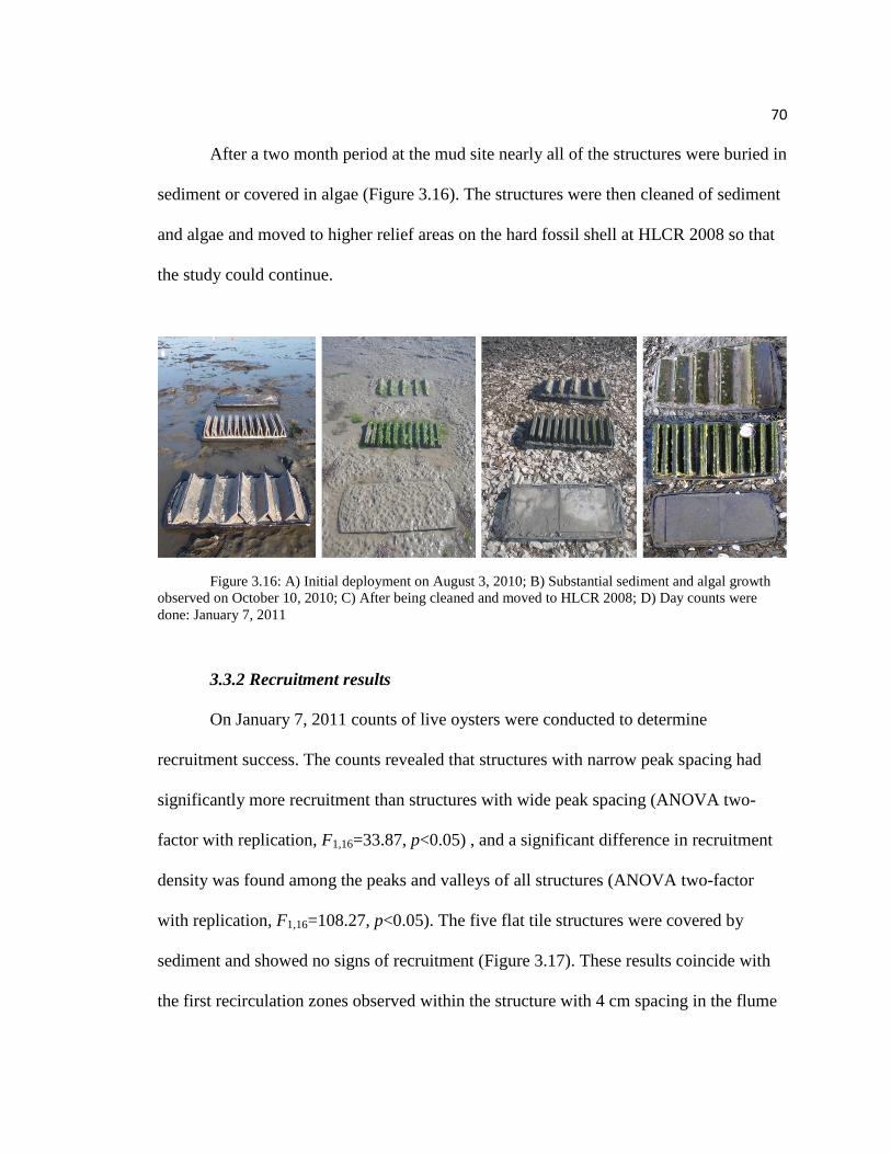
70

After a two month period at the mud site nearly all of the structures were buried in

sediment or covered in algae (Figure 3.16). The structures were then cleaned of sediment

and algae and moved to higher relief areas on the hard fossil shell at HLCR 2008 so that

the study could continue.

Figure 3.16: A) Initial deployment on August 3, 2010; B) Substantial sediment and algal growth

observed on October 10, 2010; C) After being cleaned and moved to HLCR 2008; D) Day counts were

done: January 7, 2011

3.3.2 Recruitment results

On January 7, 2011 counts of live oysters were conducted to determine

recruitment success. The counts revealed that structures with narrow peak spacing had

significantly more recruitment than structures with wide peak spacing (ANOVA two-

factor with replication, F1,16=33.87, p<0.05) , and a significant difference in recruitment

density was found among the peaks and valleys of all structures (ANOVA two-factor

with replication, F1,16=108.27, p<0.05). The five flat tile structures were covered by

sediment and showed no signs of recruitment (Figure 3.17). These results coincide with

the first recirculation zones observed within the structure with 4 cm spacing in the flume

71

study. The wide peak spacing structure in the field also had greater recruitment on the top

half, but not as much as the narrow spacing structures. The wide peak valleys had the

lowest recruitment, likely due to sediment accumulation within the valleys. Possible

reasons for the apparent preference of narrowly spaced roughness elements by oyster

larvae likely include: larvae are brought down to the substrate by the turbulence in these

zones, food is consistently delivered to settled oysters, possibly suffocating particles are

unlikely to accumulate in on steep sloping surfaces where turbulence can wash them

away, and protection from predation.

Figure 3.17: January 7, 2011 count results +/- one standard deviation for all structures; the peaks

of structures with narrowly spaced peaks had the greatest recruitment and (excluding the flat tiles) the

valleys of structures with widely spaced peaks had the least recruitment

± 5.0

± 12.7

± 33.9

± 48.7

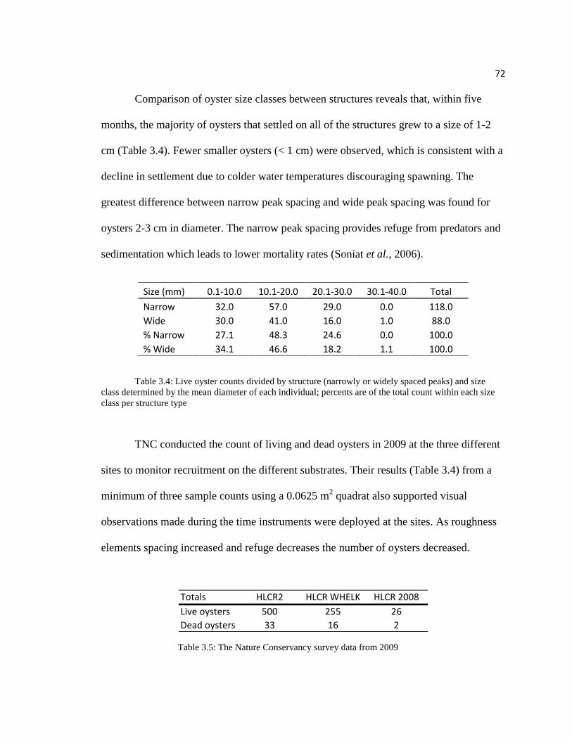
72

Comparison of oyster size classes between structures reveals that, within five

months, the majority of oysters that settled on all of the structures grew to a size of 1-2

cm (Table 3.4). Fewer smaller oysters (< 1 cm) were observed, which is consistent with a

decline in settlement due to colder water temperatures discouraging spawning. The

greatest difference between narrow peak spacing and wide peak spacing was found for

oysters 2-3 cm in diameter. The narrow peak spacing provides refuge from predators and

sedimentation which leads to lower mortality rates (Soniat et al., 2006).

Size (mm) 0.1-10.0 10.1-20.0 20.1-30.0 30.1-40.0 Total

Narrow 32.0 57.0 29.0 0.0 118.0

Wide 30.0 41.0 16.0 1.0 88.0

% Narrow 27.1 48.3 24.6 0.0 100.0

% Wide 34.1 46.6 18.2 1.1 100.0

Table 3.4: Live oyster counts divided by structure (narrowly or widely spaced peaks) and size

class determined by the mean diameter of each individual; percents are of the total count within each size

class per structure type

TNC conducted the count of living and dead oysters in 2009 at the three different

sites to monitor recruitment on the different substrates. Their results (Table 3.4) from a

minimum of three sample counts using a 0.0625 m2 quadrat also supported visual

observations made during the time instruments were deployed at the sites. As roughness

elements spacing increased and refuge decreases the number of oysters decreased.

Totals HLCR2 HLCR WHELK HLCR 2008

Live oysters 500 255 26

Dead oysters 33 16 2

Table 3.5: The Nature Conservancy survey data from 2009

73

2.4 Discussion of small scale hydrodynamics

In the Vectrino study small scale velocity measurements were taken along vertical

transects down to within 2 cm of the substrate. Vertically oriented live oysters at HLCR2

were found to form a structure that includes reduced turbulence between individual

oysters. Stresses at the healthy reef peaked at the tips of the oysters and very near to the

bed at the restoration site. Along with bed roughness, TKE dissipation decreased from

HLCR2 to HLCR 2008 to HLCR MUD. Momentum transport at HLCR2 is dominated by

turbulent sweeps reaching into the reef, whereas at HLCR 2008 ejection and sweep

events occur more equally. In a similar analysis done over a sandy benthic surface (Yuan

et al. 2009), ejection events accounted for 56% of the turbulent sediment flux from the

sandy bottom, indicating that momentum transfer is dominated by bursting events

transporting turbulent motions mostly away from a low roughness bed and is responsible

for sediment resuspension. The addition of roughness elements, as well as their density

and geometry (Hendricks et al. 2006), lead to the change in direction of momentum

transfer responsible for larval and food delivery to the bed.

A structure manipulation study was conducted to further investigate how benthic

roughness affects small-scale hydrodynamics. For both the lab flume and field studies

simplified structures of repeating vertically oriented roughness elements were constructed

to mimic benthic roughness. As discussed earlier, turbulence provides transport of the

74

larvae to the substrate (Koehl et al. 2007), and food to growing oysters (Lenihan et al.

1996). Vertical velocity profiles compared within roughness elements below the peak of

the roughness revealed two recirculation zones within the structure canopy at 4 cm

spacing and only one recirculation zone at 10 cm spacing. These areas of recirculation

match up closely to the areas where the greatest recruitment was observed on the slate tile

structures left at the field study site for five months.

In a similar study, Soniat et al. (2004) looked at statistical differences in

recruitment between narrowly spaced vertical shells, widely spaced vertical shells, and

horizontally placed shells. Their results suggest that there is no effect of vertical structure

and a negative effect of refuge on total density of oysters and on density of live oysters.

However, their results also suggest that refuge and vertical structure prevent suffocation

by sediment and predation and thus lead to lower oyster mortality. The results from this

thesis work compliment their study by revealing that drag and lift forces both increase

with roughness element spacing, but refuge area inherently decreases. Once again,

supporting results come from the recruitment study, suggesting that when natural factors

such as sedimentation and predation are included, narrowly spaced roughness elements

provide a better oyster habitat than widely spaced roughness elements or a lack of

roughness elements.

The combined field and lab results suggest that an increase in bed roughness is

beneficial for larval recruitment. Narrowly spaced, vertically oriented, repeating

roughness elements create an environment where momentum transfer is towards the bed,

75

and there are areas sheltered from intense hydrodynamics that could potentially prevent

larval settlement.

76

Chapter 4

4.1 Discussion of major findings

The heightened focus on oyster restoration and necessity to understand the

physical environment and parameters that will make restoration efforts successful were

the driving forces for this field research. Due to the expansive topic, this research focused

upon the role hydrodynamics plays in creating an environment conducive to larval

settlement success. To review, the questions addressed in this thesis were: (1) How do

elevation and bed roughness affect shear stresses and drag in the turbulent boundary layer

over an intertidal oyster reefs and restoration sites; (2) How does shear stress distribution

and variability differ among sites of varying topographies; and (3) How might the

varying hydrodynamic conditions impact larval recruitment?

Results indicate increases in bed roughness and elevation result in conditions that

support larval recruitment and oyster growth. Roughness elements provide sheltered

areas where larvae have an opportunity to settle without encountering great stresses that

may wash them away before they attach (Soniat et al. 2004, Reidenbach et al. 2009).

TKE dissipation and momentum transfer to the bed provide transport of the larvae to the

substrate (Koehl et al. 2007), food to growing oysters (Lenihan et al. 1996), flushing of

food depleted water masses (Reidenbach et al. 2007) and resuspension of sediment (Yuan

et al. 2009) from in-between oysters. Based on the Multi-site study, a site with vertical

relief (elevation) and without roughness elements does not create the same favorable

conditions for larval settlement. The mounds of fossil shell at HLCR 2008 have vertical

relief similar to the historical reef. However, high hydrodynamic stresses found very near

77

the fossil shell bed and the lack of vertically oriented roughness elements to provide

refuge from predation likely contribute to the lack of recruitment documented by TNC‘s

2009 survey (Table 3.4).

The combined results from this thesis work and the results from other studies

included in this discussion can be applied to future restoration efforts. Elevation and

benthic roughness both affect larval settlement and recruitment. Roughness elements

created artificially or the addition of large roughness, such as whelk shell, to restoration

sites would help to provide a turbulent environment for larval and food transport as well

provide areas of refuge from predators and sedimentation. Schulte et al. (2009) concluded

that vertical relief is necessary for successful recruitment to restoration efforts and Soniat

et al. (2004) concluded that vertical substrate and refuge from predation are crucial to

reef development.

4.2 Implications for restoration efforts

The investigation of the hydrodynamics of different reef structures, leads me to

conclude that elevation, benthic roughness and refuge are all factors that should be

considered in future restoration efforts.

Healthy reefs were found to have higher elevation and benthic roughness than

mud or fossil shell restoration sites. On the healthy reefs higher turbulence is created

above reef, but less along surfaces within reef where larvae may settle. The vertical

orientation of live oysters on a healthy reef also prevents sediment from accumulating

and preventing recruitment and growth.

78

Larvae prefer to settle on areas of high roughness but within the reef where bed

shear stresses are lower. The tightly packed densities of oysters on a healthy reef may

also provide protection from predation. The inclusion of whelk shell is an improvement

upon current flat oyster shell restoration sites, because of its ability to increase the

topographic variability of a restoration site as well as protected areas.

Improved restoration depends upon creating benthic substrates with densities and

roughnesses that limit sedimentation and predation. TNC is already monitoring

recruitment onto different substrates and reef structures, and they are finding greater

recruitment success on sites that contain whelk shell than on those that don‘t. The

continued use of whelk shell or the creation of beds with similar benthic topographic

variability should be the focus of future restoration efforts.

79

Acknowledgements

This opportunity to complete my first graduate level scientific research could have

been too intimidating of a task if it wasn‘t for the professional and personal assistance of

many individuals.

First of all I would like to express my appreciation to my advisory committee: Dr.

Matthew A. Reidenbach, Dr. Arthur Schwarzschild, Jerry McCormick-Ray and Dr.

Karen McGlathery. Special thanks to my primary advisor Matt Reidenbach whose time,

patience and understanding throughout this process were invaluable. He took the time to

help me start from the beginning in a new field, allowed me to learn from my mistakes

and was always available to answer my questions and concerns. The lessons I learned

from Art Schwarzschild from knot tying to last minute experimental re-design will

undoubtedly come in handy more often than I know. Jerry McCormick-Ray‘s enthusiasm

for oysters and their importance was contagious, inspiring, and a continual reminder of

the importance of this research. Karen McGlathery helped me take the critical step to

conduct my research so that it was meaningful beyond just my study site.

My field research would not have been possible without the supportive staff of the

Anheiser Busch Coastal Research Center at the Virginia Coastal Reserve LTER, my

fellow graduate students and lab mates, many who offered field assistance, and The

Nature Conservancy. J.C.R. (Jenny) Hansen was my partner in the field, my personal

Matlab tutor, and often times emotional support and the all important comic relief. James

Selph, a high school student, whom I was partnered with through the Research

80

Experience for High School students (REHS) program, assisted me in data collection

during the summer of 2009. Thanks go to The Nature Conservancy for allowing me to

conduct my research on their protected land and the supervision and assistance of Barry

Truitt and Bo Lusk.

My laboratory research made possible by funding from the University of Virginia‘s

Exploratory Research Award, Gerald Williamson‘s time and efforts in the machine shop

constructing the recirculating flume, and Kathleen Walsh who spent many hours in the

lab re-running experiments as we learned from our mistakes.

My personal experience during my time at the University of Virginia was enriched

by my relationships with fellow graduate students, the Environmental Sciences faculty

and staff, and my great friends. Jenny, Jenn H., Abi, Kirby, Jenn B, Katy, Neg and Rowe

were there for me in countless ways over the past three years. Finally, I must

acknowledge my family‘s support, especially my mother Linda Gardner who has paved

the road that continues to lead me to great places and whose love and support is always

just a phone call away.

This research was funded by a Virginia Coast Reserve Long Term Ecological

Research grant by the National Science Foundation (NSF-DEB 0621014), University of

Virginia, and the REHS program.

81

References

Arve, J. (1960). Preliminary report on attracting fish by oyster-shell plantings in

Chincoteague Bay, Maryland. Chesapeake Science, 1(1), 58-65.

Bahr, L., & Lanier, W. (1981). The ecology of intertidal oyster reefs of the south Atlantic

coast: A community profile. US Fish and Wildlife FWS/OBS/81.15, Washington,

DC, USA,

Bartol, I. K., Mann, R., & Luckenbach, M. (1999). Growth and mortality of oysters

(Crassostrea virginica) on constructed intertidal reefs: Effects of tidal height and

substrate level. Journal of Experimental Marine Biology and Ecology, 237(2), 157-

184.

Bennet, S. J., and J. L. Best (1996), Mean flow and turbulence structure over fixed ripples

and

the ripple‐dune transition, in Coherent Flow Structures in Open Channels, edited by

P. J. Ashworth et al., pp. 281–304, John Wiley, New York.

Bergeron, N. E., & Abrahams, A. D. (1992). Estimating shear velocity and roughness

length from velocity profiles. Water Resources Research, 28(8), 2155-2158.

Brumbaugh, R. D., Sorabella, L. A., Garcia, C. O., Goldsborough, W. J., & Wesson, J. A.

(2000). Making a case for community-based oyster restoration: An example from

hampton roads, Virginia, U. S. A. Journal of Shellfish Research, 19(1), 467-472.

Bushek, D. (1988). Settlement as a major determinant of intertidal oyster and barnacle

distributions along a horizontal gradient. Journal of Experimental Marine Biology

and Ecology, 122(1), 1-18.

Carriker, M., Gaffney, P., Kennedy, V., Newell, R., & Eble, A. (1996). The eastern

oyster: Crassostrea virginica. Kennedy VS, Newell RIE, Eble AF A Catalogue of

Selected Species of Living Oysters of the World.Maryland Sea Grant College

Program, College Park,

Cerco, C. F., & Noel, M. R. (2007). Can oyster restoration reverse cultural eutrophication

in Chesapeake Bay? Estuaries and Coasts, 30(2), 331-343.

Cheng, R. T., Ling, C. H., Gartner, J. W., & Wang, P. (1999). Estimates of bottom

roughness length and bottom shear stress in South San Francisco Bay, California.

Journal of Geophysical Research, 104(C4), 7715-7728.

82

Coen, L. D., & Luckenbach, M. W. (2000). Developing success criteria and goals for

evaluating oyster reef restoration: Ecological function or resource exploitation?

Ecological Engineering, 15(3-4), 323-343.

Crimaldi, J. P., Thompson, J. K., Rosman, J. H., Lowe, R. J., & Koseff, J. R. (2002).

Hydrodynamics of larval settlement: The influence of turbulent stress events at

potential recruitment sites. Limnology and Oceanography, 47(4), 1137-1151.

Dame, R. F., Zingmark, R. G., & Haskin, E. (1984). Oyster reefs as processors of

estuarine materials*. Journal of Experimental Marine Biology and Ecology, 83(3),

239-247.

Dennison, W. C., & Alberte, R. S. (1985). Role of daily light period in the depth

distribution of Zostera marina(eelgrass). Marine Ecology Progress Series.Oldendorf,

25(1), 51-61.

Eckman, J., Savidge, W., & Gross, T. (1990). Relationship between duration of cyprid

attachment and drag forces associated with detachment of Balanus amphitrite

cyprids. Marine Biology, 107(1), 111-118.

Fréchette, M., Butman, C. A., & Geyer, W. R. (1989). The importance of boundary-layer

flows in supplying phytoplankton to the benthic suspension feeder, Mytilus edulis L.

Limnology and Oceanography, 34(1), 19-36.

Fuchs, H. L., Neubert, M. G., & Mullineaux, L. S. (2007). Effects of turbulence-mediated

larval behavior on larval supply and settlement in tidal currents. Limnology and

Oceanography, 52(3), 1156-1165.

Galtsoff, P. S. (1964). The american oyster crassostrea virginica gmelin. Fishery Bulletin

Grass, A. (1971). Structural features of turbulent flow over smooth and rough boundaries.

Journal of Fluid Mechanics, 50(02), 233-255.

Gross, T. F., & Nowell, A. R. M. (1983). Continental Shelf Research, 2(2-3), 109-126.

Hadfield, M. (2007). Individual-based model of larval transport to coral reefs in

turbulent, wave-driven flow: Behavioral responses to dissolved settlement inducer.

Mar Ecol Prog Ser, 335, 1-18.

Harwell, M. C., & Orth, R. J. (1999). Eelgrass (Zostera marina L.) seed protection for

field experiments and implications for large-scale restoration. Aquatic Botany, 64(1),

51-61.

83

Haven, D. S., & Morales-Alamo, R. (1966). Aspects of biodeposition by oysters and

other invertebrate filter feeders. Limnology and Oceanography, 11(4), 487-498.

Hendriks, I. E., Van Duren, L. A., & Herman, P. M. J. (2006). Turbulence levels in a

flume compared to the field: Implications for larval settlement studies. Journal of

Sea Research, 55(1), 15-29.

Jonsson, P., van Duren, L., Amielh, M., & Asmus, R. Making water flow: A comparison

of the hydrodynamic characteristics of 12 different benthic biological flumes.

Aquat.Ecol, 40, 409–438.

Kemp, W., Boynton, W., Adolf, J., Boesch, D., Boicourt, W., Brush, G., et al. (2005).

Eutrophication of Chesapeake Bay: Historical trends and ecological interactions.

Marine Ecology Progress Series, 303, 1-29.

Kennedy, V., & Krantz, L. (1982). Comparative gametogenic and spawning patterns of

the oyster Crassostrea virginica (gmelin) in central Chesapeake Bay. J.Shellfish Res,

2(2), 133-140.

Koehl, M., & Hadfield, M. (2004). Soluble settlement cue in slowly moving water within

coral reefs induces larval adhesion to surfaces. Journal of Marine Systems, 49(1-4),

75-88.

Koehl, M. (2007). Mini review: Hydrodynamics of larval settlement into fouling

communities. Biofouling, 23(5), 357-368.

Koehl, M.A.R. and M. Hadfield. (2010) Hydrodynamics of larval settlement from a

larva‘s point of view. Integr. Comp. Biol. 50 : 539-551.

Krause-Jensen, D., Sagert, S., Schubert, H., & Boström, C. (2008). Empirical

relationships linking distribution and abundance of marine vegetation to

eutrophication. Ecological Indicators, 8(5), 515-529.

Lacey, R. W. J., & Roy, A. G. (2008). Fine-scale characterization of the turbulent shear

layer of an instream pebble cluster. Journal of Hydraulic Engineering, 134, 925.

Lenihan, H. S., & Peterson, C. H. (1998). How habitat degradation through fishery

disturbance enhances impacts of hypoxia on oyster reefs. Ecological Applications,

8(1), 128-140.

Lenihan, H. S., Peterson, C. H., & Allen, J. M. (1996). Does flow speed also have a direct

effect on growth of active suspension-feeders: An experimental test on oysters.

Limnology and Oceanography, 41(6), 1359-1366.

84

Lenihan, H. S. (1999). Physical–biological coupling on oyster reefs: how habitat structure

influences individual performance. Ecological Monographs, 69(3), 251-275.

Loosanoff, V. L. (1965). Gonad development and discharge of spawn in oysters of long

island sound. Biological Bulletin, 129(3), 546-561.

Lu, S., & Willmarth, W. (1973). Measurements of the structure of the Reynolds stress in

a turbulent boundary layer. Journal of Fluid Mechanics, 60(03), 481-511.

McCormick-Ray, M. G. (1998). Oyster reefs in 1878 seascape pattern—Winslow

revisited. Estuaries and Coasts, 21(4), 784-800.

MacKenzie, C. (1983). To increase oyster production in the northeastern united states.

Marine Fisheries Review, 45(3), 1-22.

McGlathery, K. J. (2001). Macroalgal blooms contribute to the decline of seagrass in

nutrient‐enriched coastal waters. Journal of Phycology, 37(4), 453-456.

Michael Kemp, W., Batleson, R., Bergstrom, P., Carter, V., Gallegos, C. L., Hunley, W.,

et al. (2004). Habitat requirements for submerged aquatic vegetation in Chesapeake

Bay: Water quality, light regime, and physical-chemical factors. Estuaries and

Coasts, 27(3), 363-377.

Nelson, K. A., Leonard, L. A., Posey, M. H., Alphin, T. D., & Mallin, M. A. (2004).

Using transplanted oyster (Crassostrea virginica) beds to improve water quality in

small tidal creeks: A pilot study. Journal of Experimental Marine Biology and

Ecology, 298(2), 347-368.

Newell, R. I. E., Kemp, W. M., Hagy, J., Cerco, C. F., Testa, J. M., & Boynton, W. R.

(2007). Top-down control of phytoplankton by oysters in Chesapeake Bay, USA:

Comment on Pomeroy et al.(2006). MARINE ECOLOGY-PROGRESS SERIES-, 341,

293.

Newell, R. (1988). Ecological changes in Chesapeake Bay: Are they the result of

overharvesting the American oyster, Crassostrea virginica. Understanding the

Estuary: Advances in Chesapeake Bay Research, 129, 536–546.

Newell, R., Alspach, G., Kennedy, V., & Jacobs, D. (2000). Mortality of newly

metamorphosed eastern oysters (Crassostrea virginica) in mesohaline Chesapeake

Bay. Marine Biology, 136(4), 665-676.

Orth, R. J., Luckenbach, M. L., Marion, S. R., Moore, K. A., & Wilcox, D. J. (2006).

Seagrass recovery in the delmarva coastal bays, USA. Aquatic Botany, 84(1), 26-36.

85

Pomeroy, L. R., D Elia, C. F., & Schaffner, L. C. (2007). Top-down control of

phytoplankton by oysters in chesapeake Bay, USA: Reply to newell et al.(2007).

Marine Ecology Progress Series, 341, 299-301.

Pomeroy, L. R., D'Elia, C. F., & Schaffner, L. C. (2006). Limits to top-down control of

phytoplankton by oysters in Chesapeake Bay. Marine Ecology Progress Series, 325,

301-309.

Reidenbach, M. A., Koseff, J. R., & Koehl, M. (2009). Hydrodynamic forces on larvae

affect their settlement on coral reefs in turbulent, wave-driven flow.

Limnol.Oceanogr, 54(1), 318-330.

Reidenbach, M. A., Koseff, J. R., & Monismith, S. G. (2007). Laboratory experiments of

fine-scale mixing and mass transport within a coral canopy. Physics of Fluids, 19,

075107.

Rothschild, B., Ault, J., Goulletquer, P., & Heral, M. (1994). Decline of the Chesapeake

Bay oyster population: A century of habitat destruction and overfishing. Marine

Ecology Progress Series.Oldendorf, 111(1), 29-39.

Schulte, D. M., Burke, R. P., & Lipcius, R. N. (2009). Unprecedented restoration of a

native oyster metapopulation. Science, 325(5944), 1124.

Thompson, R. J., R.I.E. Newell, V.S. Kennedy, and R. Mann. 1996. Reproduction and

Larval Development. Pages 335-370, Chapter 9 In: V.S. Kennedy, R.I.E. Newell and

A. Eble (eds.). The Eastern Oyster, Crassostrea virginica. Maryland Sea Grant

Publication.

Wethey, D. S. (1986). Ranking of settlement cues by barnacle larvae: Influence of

surface contour. Bulletin of Marine Science, 39(2), 393-400.

Wiberg, P. L., & Smith, J. D. (1985). A theoretical model for saltating grains in water.

Journal of Geophysical Research, 90(C4), 7341-7354.

Wiberg, P. L., & Smith, J. D. (1987). Calculations of the critical shear stress for motion

of uniform and heterogeneous sediments. Water Resources Research, 23(8), 1471-

1480.

Wildish, D., & Kristmanson, D. (1979). Tidal energy and sublittoral macrobenthic

animals in estuaries. Journal of the Fisheries Research Board of Canada, 36(10)

Yuan, Y., Wei, H., Zhao, L., & Cao, Y. (2009). Implications of intermittent turbulent

bursts for sediment resuspension in a coastal bottom boundary layer: A field study in

the western yellow sea, china. Marine Geology, 263(1-4), 87-96.

86

Zimmerman, R., Minello, T., Baumer, T., & Castiglione, M. (1989). Oyster reef as

habitat for estuarine macrofauna. National Oceanic and Atmospheric Administration

Technical Memorandum NMFS-SEFC-249

87

Appendix I

Suspended sediment

To determine suspended sediment concentrations optical backscatter recorders

(OBS, Campbell Scientific OBS3+©), sampling simultaneously used to collect

suspended particle data. OBS recorders are connected to ADVs and AQDPs whenever

they are deployed. The data is recorded using the internal memory of the ADVs and

AQDPs. Since the measurement volume for the OBSs are unknown the deployment

technique was changed from upward facing for all deployments in 2009 to downward

facing for all deployments in 2010. When deployed with ADVs the OBSs were always

deployed facing downward from the aluminum frame.

The analysis of the OBS sediment data is dependent upon ambient sediment

properties, so correlation curves were empirically derived for each OBS. Sediment was

collected from HLCR 2008, HLCR WHELK, HLCR MUD, and on either side of

HLCR2. The pairing of OBS‘ and instruments was kept constant among experiments so

that correlation curves were created using the instrument (AQDP or ADV) and OBS.

Three 10 ml subsamples of water were collected, filtered, dried, and weighed to get the

average background starting concentration. Enough water was added to the collected

sediment to turn it into very wet mud. Again, three 10 ml subsamples of this were

collected and analyzed in the same manner as the water. For each combination the

instrument and OBS were placed in a clean (i.e., no added sediment) salt water for

approximately 30 seconds. 1 TBS (14.79 ml) of the well-mixed corresponding mud

88

mixture was then added and well mixed with into the container of water and a

measurement was taken from the OBS. With the instruments taken completely out of the

water in between, 1 TBS of mud slurry was added at a time for up to 2.5 cups (591 ml).

The 30 second data recordings from the OBS were averaged to come up with one data

point for each known sediment concentration. A best fit line was fit to all of the data

points for each of the instrument combinations to create correlation curves (Figure A.I.1).

Figure A.I.1: Sample correlation curve for OBS #T8338 and paired AQDV; All curves had an R2

value greater than 0.99, so there is a high level of confidence in the calibration.

Sediment dynamics and filtration by the oyster community

In the first of several large scale flow experiments, bulk flow across the reef was

measured and the net effect of the reef on suspended sediment was quantified. The

instrumentation used in this study collected data regarding how the vertical relief of the

historical reef, HLCR2, influences water column turbulence and mean flow rates and how

89

the filtering capacity of the oysters affects suspended sediment levels and sedimentation.

Figure A.I.2 depicts the instrumentation of the reef for the sediment filtration experiment.

Large scale flow patterns across the reef were measured by placing ADVs at locations on

either side of the reef and an AQDP on top of the reef, along a horizontal transect,

aligned as best as possible with the dominant flow direction.

Figure A.I.2: Instruments aligned with the dominant flow to study how the vertical relief of the

reef influences bulk flow, and to determine the effects of filtration on sediment uptake by the reef

Velocity data from the two ADVs was plotted together with time to identify

differences between the flow upstream and downstream of the reef. Differences between

the two during ebb, flood, and slack tides were focused on to identify any patterns. To

determine the affects of the reef on suspended sediment concentrations three optical

backscatter recorders (OBS), sampling simultaneously, were collected suspended particle

data. These OBS sensors were connected to and data was recorded by each of the two

ADVs flanking the oyster reef and the AQDP located at the center of the reef. Sediment

uptake by the filtering of the reef was approximated using differencing of the upstream

90

and downstream sediment measurements along the dominant flow path. A negative

difference between the downstream and upstream OBS‘ indicates a net uptake of

sediment by the oysters, whereas a positive difference indicates a net resuspension by the

bed. Figure A.I.3-D shows the concentration gradient between the east and west sides of

the oyster reef.

Time [Julian Day]

Figure A.I.3: (A) Velocities west of oyster reef. (B) Velocities east of oyster reef. (C) Water depth

above reef. (D) Suspended sediment concentration gradient between the west and east side of the oyster

reef.

91

Figure A.I.4 shows that net uptake of sediment by the reef community increased

with increasing mean velocity. Greater flow speeds lead to greater vertical mixing that

provides a constant supply of water containing food, and prevents a layer of seston

depleted water at the reef‘s surface (Wildish and Kristmanson 1979, Frechette et al. 1989,

Lenihan et al. 1996). The feeding oysters under these conditions have access to more of

the water column, and have the opportunity to filter more suspended sediment along with

their food.

Figure A.I.4: Sediment uptake as a function of mean velocity across the oyster reef; Uptake rate

was calculated using the difference between upstream and downstream sediment concentrations.

In the suspended solids study, SSC was recorded both upstream and downstream

of HLCR2. The effect of the oyster community at HLCR2 on SSC appeared to be

depletion of SSC as the water flowed over the reef. This may be a result of active

filtration by the feeding oysters that, on a small scale, has been documented in other

studies (e.g. Nelson et al., 2004; Porter et al., 2004; Cerco and Noel, 2007). However, if

92

the depletion of suspended solids by one oyster reef could be scaled up to a bay size area

the benefits to oyster reef restoration could be substantial (Newell 1988, Newell et al.

2007). Pomeroy et al., (2006 and 2007) disputes the theory that oyster restoration to

historical masses would be capable of directly controlling phytoplankton blooms, but the

affects of oyster filtration observed in this study would likely impact adjacent ecosystems

such as seagrass meadows and species that depend on them. Aquatic vegetation including

Zostera marina, the seagrass species that is the focus of a massive restoration effort in the

coastal bays of the Delmarva Peninsula (Harwell and Orth 1999, Orth et al 2006), has a

minimum light requirement for growth and survival (Kemp et al. 2004). The depletion of

suspended solids and nutrients, provided by adjacent oyster reefs, would allow light to

penetrate deeper into the water column which would increase the depth distribution and

density of seagrass (Dennison and Alberte 1985, Krause-Jensen et al. 2000, McGlathery

2001) would create a positive feedback for seagrass growth. However, given current

oyster populations it is unlikely that they exert a strong control on bulk SSC

concentrations within the coastal bays.

93

Appendix II

AQDP plots

Dominant flow was consistently observed coming from the channel, across the

site in a Northeast/Southwest direction. When the water is still relatively deep, a strong

southerly current is present. At all sights velocities drop to 0 cm/s during slack tide.

Elevation

Figure A.II.1: East velocities over 5 consecutive tidal cycles taken simultaneously at 3 elevations

94

Figure A.II.1: North velocities over 5 consecutive tidal cycles taken simultaneously at 3 elevations

95

Various bed substrates: Multi-site study

Figure A.II.3: East velocities over five consecutive tidal cycles taken simultaneously at the four sites

96

Figure A.II.4: North velocities over five consecutive tidal cycles taken simultaneously at the four sites

abstract - university of virginia

Documents