abstract title of thesis: uncertainty analysis and …
TRANSCRIPT

ABSTRACT
Title of Thesis: UNCERTAINTY ANALYSIS AND QUALITY
ASSURANCE FOR COORDINATE MEASURING
SYSTEM SOFTWARE
Bonnie Lawford, Master of Science, 2003
Thesis Directed by: Professor Linda SchmidtDepartment of Mechanical Engineering
Coordinate measuring systems are installed worldwide in factories, research and
medical labs, and other industrial facilities. The purpose of the machines is to
estimate how much a measured part deviates from the corresponding perfect
geometry. The accuracy of the results is limited by, among other things, faulty CMS
software with unknown measurement uncertainty. A record and understanding of this
information is vital to industry for good results. This thesis serves as a repository and
comprehensive overview of the problems with CMS software and approaches taken
to solving those problems. The paper also covers new work done by the author in the
areas of reference algorithm testing and verification, industry software testing via
inter-comparisons with the reference algorithms, and solutions to problems similar
but not identical to the fitting problems encountered in the past.

UNCERTAINTY ANALYSIS AND QUALITY ASSURANCE FOR
COORDINATE MEASURING SYSTEM SOFTWARE
by
Bonnie Lawford
Thesis submitted to the Faculty of the Graduate School of the University of Maryland, College Park in partial fulfillment
of the requirements for the degree of Master of Science
2003
Advisory Committee:
Professor Linda Schmidt, ChairDr. Craig ShakarjiProfessor Guangming Zhang


ii
ACKNOWLEDGEMENTS
The guidance and support of Dr. Craig Shakarji and Dr. Linda Schmidt have been
invaluable throughout my research and study. This work would not be possible
without their efforts and insights.

iii
TABLE OF CONTENTS1. INTRODUCTION .................................................................................................... 1
1.1 Coordinate Measuring Systems .......................................................................... 11.2 The Problem of Uncertainty................................................................................ 41.3 The Problem of Software Uncertainty ................................................................ 61.4 The NIST ATEP-CMS software testing program............................................. 11
2. BACKGROUND INFORMATION AND LITERATURE SURVEY................... 142.1 NIST work ........................................................................................................ 142.2 NIST Algorithm Information............................................................................ 172.3 NPL work.......................................................................................................... 212.4 Other documentation......................................................................................... 24
3. LEAST SQUARES FITTING ................................................................................ 263.1 The Problem of Least Squares Fitting .............................................................. 263.2 The Need for Least Squares Fitting .................................................................. 273.3 Issues involved in solving Least Squares Fitting Problems.............................. 273.4 An Approach to Least Squares Fitting.............................................................. 283.5 Implementation of the Approach ...................................................................... 283.6 Results of the Implementation .......................................................................... 293.7 An Application of Least Squares Fitting .......................................................... 29
4. MINIMUM ZONE FITTING ................................................................................. 394.1 The Problem of Minimum Zone Fitting............................................................ 394.2 The Need for Minimum Zone Fitting ............................................................... 404.3 Issues involved in solving Minimum Zone Fitting Problems........................... 424.4 An Approach to Solving Minimum Zone Fitting ............................................. 434.5 Implementation of the Approach ...................................................................... 444.6 Reference vs. Commercial Algorithm Performance......................................... 464.7 Results of the Implementation .......................................................................... 48
5. MAXIMUM INSCRIBED AND MINIMUM CIRCUMSCRIBED FITTING...... 495.1 The Problem of Maximum Inscribed and Minimum Circumscribed Fitting.... 495.2 The Need for Maximum Inscribed and Minimum Circumscribed Fitting........ 515.3 Issues involved in solving Maximum Inscribed and Minimum Circumscribed Fitting Problems...................................................................................................... 525.4 An approach to Maximum Inscribed and Minimum Circumscribed Fitting .... 535.5 Implementation of the Approach ...................................................................... 595.6 Reference vs. Commercial Algorithms for Maximum Inscribed and Minimum Circumscribed Fitting ............................................................................................. 595.7 Results of the Implementation .......................................................................... 61
6. LEAST SQUARES FITTING OF COMPLEX SURFACES................................. 626.1 The Problem of Least Squares Fitting of Complex Surfaces............................ 626.2 The Need for Fitting of Complex Surfaces....................................................... 636.3 Issues involved in solving Least Squares Fitting of Complex Surfaces Problems................................................................................................................................. 646.4 An Approach to Solving Least Squares Fitting of Complex Surfaces Problems................................................................................................................................. 686.5 Implementation of the Approach ...................................................................... 696.6 Results of the Implementation .......................................................................... 77

iv
7. OTHER ISSUES AND FUTURE WORK ............................................................. 787.1 Other Issues Involved in CMS Fitting Software............................................... 787.2 Future Work ...................................................................................................... 79
8. Conclusions............................................................................................................. 81REFERENCES ........................................................................................................... 87

v
LIST OF TABLES
Table 2.1. Geometries for which the new NIST reference algorithms can be utilized.............................................................................................................................. 20
Table 4.1. Results of Minimum Zone Fit Testing....................................................... 47Table 5.1a. Results from exhaustive search engine .................................................... 55Table 5.1. Results for simulated annealing/exhaustive search validation test. ........... 55Table 5.3. Minimum Circumscribed Fit Results......................................................... 60Table 5.2. Maximum Inscribed Fit Results................................................................. 60

vi
LIST OF FIGURES
Figure 1.1. Examples of different types of CMSs: 1) CMM, 2) theodolite, and 3) photogrammetry. ................................................................................................... 3
Figure 1.2. The various fit types for (a) circular data with 3-lobed form error and (b) data for a plane...................................................................................................... 7
Figure 2.1. The Architecture of the NIST Algorithm Testing Service [18] .............. 16Figure 3.1 A picture of the matrix transducer used in the non-destructive spot weld
detector application............................................................................................. 30Figure 3.2. Building the image of the welded area: the software uses the transducer
output and creates a grid, shown on the right, that is translated into numerical values representing the amount of weld material present in each grid space. .... 31
Figure 3.3. An example of an output grid where the number in each grid space represents the amount of spot-weld present in that cell. ..................................... 31
Figure 3.4. An illustration of the division of the problem space into four regions..... 33Figure 3.5. Four examples of the third case scenario where R < y max and R > y min.
............................................................................................................................. 34Figure 3.6. Two pictures illustrating the fourth case scenario, where y min > R < y
max...................................................................................................................... 35Figure 3.7. Another example of case four (y min > R < y max). ................................ 35Figure 4.1. Minimum Zone fit for circle data. Note that the dimensions of the
resulting circle will be similar, but generally not identical to the least squares fit circle.................................................................................................................... 40
Figure 4.2. Minimum zone circles: the figure on the left shows the minimum circumscribed and maximum inscribed fits for the circle data, the figure on the right is the minimum zone fit. The fits form concentric circles.......................... 41
Figure 4.3. Function with local minima that may pose problems for a “downhill only” minimization function......................................................................................... 42
Figure 5.1. Chebyshev fits for a set of circle data. The circle on the left illustrates the minimum circumscribed fit while the circle on the left illustrates the maximum inscribed fit. ........................................................................................................ 50
Figure 5.2. (a) Maximum inscribed and (b) minimum circumscribed fits for cylinder data. ..................................................................................................................... 51
Figure 5.3. Two problematic geometries: (a) a surfaces with 2 equal solutions and (b) a surface with two local minimum solutions but only one true global minimum.............................................................................................................................. 53
Figure 6.1. Two examples of complex surfaces displayed using computer graphics. 62Figure 6.2. An application of geometric fitting of complex surfaces. ........................ 64Figure 6.3. A problematic complex surface; the corner points may be mapped to
either planar surface, not necessarily the correct corresponding plane. ............. 65

1
1. INTRODUCTION
1.1 Coordinate Measuring Systems
Coordinate measuring systems (CMSs) are installed in factories, research and medical
labs, as well as many other industrial and scientific facilities. The definition of a CMS
is, "…any piece of equipment which collects coordinates (points) and calculates and
displays additional information using the measured points," [8]. To find the
dimensions of a part, a CMS measures point locations on the object’s surface. This
coordinate data is then processed to determine the part’s dimensions and the types
and locations of variations in the surface. Note that the raw coordinate data generally
must be interpreted before the information gathered is of any real use. Specifically,
once the coordinate data points are collected from the surface of the part by the CMS
hardware, the information is processed by software, which usually performs a
geometric fit to the gathered data. This fitting software, which is usually integrated as
part of the CMS, uses the coordinate data to, for instance, determine a part’s location,
orientation, concentricity, or deviation of the part from the corresponding perfect
geometry. The software can apply appropriate processing of the data to determine if a
part is within tolerances defined in specifications. Since a part is measured through
only a sampling of points, its true surface can never be known exactly; instead, an
approximation of the surface is known based on a finite sampling of coordinate
points. The software will often be required to compute a “substitute geometry” based
on the imperfect data. This substitute geometry is a perfect, theoretical, mathematical
shape fit to the points. For example if a CMS samples points on a surface that is

2
nominally cylindrical, then the software can compute a fit to find the “best” perfect
cylinder that is represented by the imperfectly measured points on the imperfect
physical surface. Just how this substitute feature is determined can be complicated
and is discussed in this paper.
CMSs are used to measure everything from pistons and cylinders to gears and screw
threads to airplane wings and car doors. Sometimes their uses go beyond
manufactured parts to include, for example, bones and vertebrae alignment in the
medical field. Many different types of coordinate measuring systems are in use today
including theodolites, photogrammetry, optical systems, and coordinate measuring
machines. Though such variation exists among CMSs, the software packages that
they normally come equipped with are similar and share some basic problems and
issues. Examples of several different types of systems are given1 in figure 1.1. Shown
in the pictures are: 1) CMM: a measuring system with the means to move a probing
system and capable of determining spatial coordinates on a workpiece surface, 2)
theodolite: a small telescope mounted and moving on two graduated circles, one
horizontal, the other vertical, while its axes pass through the center of the circles. The
data points are found using triangulation, and 3) photogrammetry: this system works
by taking pictures of the object being measured with a digital camera then inputting
the image into the software to determine its part information.
1 Disclaimer: Certain work described in this paper was done in conjunction with NIST. Certain commercial equipment, instruments, or materials are identified in this paper to foster understanding. Such identification does not imply recommendation or endorsement by the National Institute of Standards and Technology, nor does it imply that the materials or equipment identified are necessarily the best available for the purpose.

3
Since their invention, much research and development has been done to enhance the
measurement accuracy of CMSs. Much of that work has been to make the individual
point measurements more accurate. Today, CMS hardware can perform to a high
degree of precision to meet increasingly high tolerances used in manufacturing. For
instance, many CMMs can compute a point-to-point length measurement that is
nominally a meter in length (under ideal conditions) with an uncertainty (giving 95%
confidence) of less than a micrometer.
Yet there still remains a major source of uncertainty that often goes unchecked, that
source being the fitting software that analyzes the collected data points and interprets
the data in a manner needed by the CMS user. This software is often problematic and
thus it can often lead to erroneous results [44, 22, 23]. Companies write software for
installation in CMSs, the inner workings of which are proprietary and therefore
hidden from the user. Some black box testing of this fitting software is therefore
Figure 1.1. Examples of different types of CMSs: 1) CMM, 2) theodolite, and 3) photogrammetry.

4
necessary to determine their performance characteristics, which testing is discussed in
this paper.
1.2 The Problem of Uncertainty
1.2.1 Theoretical versus Actual Geometries
Once the part has been designed and modeled mathematically it can then be
manufactured. Machine tools are used to transform a piece of raw material into the
desired geometry with the specified dimensions. Some computer aided tools might be
used, or the part may be hand-made using machining hardware. The mathematical
model is used as a guide to manufacturing the part.
In the process of manufacturing, however, imperfections in the machine tools, the raw
material, and the machining environment cause geometric deviation from that ideal,
mathematically defined geometry. Both random and systematic (i.e., consistently
recurring) effects cause the variations resulting from the various manufacturing
systems. The types, amounts, and locations of the errors vary for each part created on
each machine. The purpose of coordinate measuring systems is to determine the final
dimensions of the manufactured part and to provide information about the errors that
are present.
1.2.2 Types of Errors

5
We live in an imperfect world. In the material realm there is no such thing as a
perfectly flat plane or a perfectly spherical ball. Some degree of imperfection exists in
all manufactured objects. For our purposes, the discussion of such imperfection, or
error, will cover two particular error types.
The first type of error, called form error, conveys the idea that parts are not perfectly
the shape of their nominal geometry. Even if the measuring equipment were
somehow perfect, the point measurements would generally still deviate from the
nominally perfect shape. While the design engineers might have called for a perfectly
round part, the manufacturing process (e.g. casting, milling, etc.) does not result in a
perfect object. Some form error can be expected in any manufactured part.
The second type of error, called measurement error, arises when data points are
collected on the surface of an object. Sources of error in the measurement equipment
(axial bends in some hardware, probe system imperfections, fixturing, etc.) and the
measurement environment (temperature, vibration, etc.) lead to inaccuracies in the
measured points.
These two types of error exist in all real-world measurement scenarios. Even if one
had a ‘golden mill’ on which to create a perfect planar surface, the measuring of it
would produce planar data that was close to a perfect plane but had some
measurement error present. Similarly, if one had a ‘golden CMS’ rather than a golden
mill, and therefore could eliminate all measurement error and know some exact,

6
actual coordinate data points located on the surface, we would not expect it to
measure points exactly on a mathematically perfect geometry, as there would be form
errors in the part. Actually, in illustrating both of the above cases, a ‘golden engineer’
is also needed to operate the machines since human interaction is yet another source
(sometimes even the largest source) of error.
1.3 The Problem of Software Uncertainty
A possibly significant component of the overall measurement uncertainty is the
contribution due to the embedded software algorithms that fit mathematical
definitions of surfaces to the coordinate data [44, 40]. Before the software processing,
data points measured by the CMS are more or less unintelligible, as they are simply a
long list of (x, y, z) coordinate points. It is the job of the CMS fitting software to
process the data in such a way that it will be useful to the user. It does this by finding
the geometric model that most closely fits the given data set based on the criterion
defined by the CMS user. This fit objective may be least squares, minimum zone
(also referred to as mini-max or the Chebyshev best fit), minimum circumscribed, or
maximum inscribed. (These fitting criteria are discussed in detail in following
chapters).

7
To illustrate these different fit objectives, an example of some CMS coordinate data
for a circular part is shown in figure 1.2(a), the data can be interpreted or ‘fit’ in a
least squares sense, a minimum zone sense, a maximum inscribed sense, or a
minimum circumscribed sense. The same can be true for a horizontal plane, shown in
figure 1.2(b). (Technically, maximum inscribed and minimum circumscribed criteria
do not apply to the fitting of planes, but these are included in the figure to highlight
the conceptual differences in the objectives). Fitting the data in different ways yields
drastically different resulting geometries. The software will normally include
information about the location, orientation, size, and form of the part, as well as any
other parameters needed to define the calculated fit (i.e., the substitute geometry). The
(signed) distances from the data points to the substitute geometry are called residuals.
In addition to the above information, the CMS software will usually provide the
Figure 1.2. The various fit types for (a) circular data with 3-lobed form error and (b) data for a plane.

8
maximum and minimum residuals. The processed results are then analyzed to
determine part quality, specifically in relation to specified part tolerances (size, form,
orientation with respect to other geometric features, location, etc.)
Finding the optimum solution based on any of these mentioned criteria is equivalent
to minimizing an appropriate objective function. Geometric fitting is really an
optimization problem in its purest form, where the problem is to find the parameters
of the substitute geometry that optimize the appropriate objective function [11].
Which fit objective to use in what situations is by no means an easy question to
answer. If the fit objective is not specified, the user must take into account the
properties of the choice of objective function in relation to the requirements of the
part. Table 1.1 summarizes four common fit objectives, along with their
characteristics. The table is a guideline—it is not intended to definitively answer what
fit objective is appropriate in any given situation. Expanded descriptions of these four
fit types are given in following chapters.

9
Table 1.1. Some of the Pros and cons of the different fit types and when to use them.
Assuming the user has chosen the appropriate fit objective, the problem of evaluating
the uncertainty due to software still looms. One of the main topics of this thesis deals
with the problem of significant uncertainty due to fitting software (even when using
the correct fit type for the problem at hand). Even when the mathematical problem is
well-defined optimization, and even when the errors in the measured data points are
not considered, the threat of significant uncertainty due to incorrect optimizations is
real [44, 40].
Least Squares Minimum Zone Minimum Circumscribed
Maximum Inscribed
Pros/Cons/
Other Issues
- Most Stable Random noise is filtered out
- Easy & Fast
- Most CMSs come equipped with it.
- Well-researched/ well understood
- Minimizes the maximum residual
- Highly influenced by outliers and random noise
- Finds smallest diameter that envelopes all the data points.
- Highly influenced by outliers and random noise
- Finds largest diameter that is inside all data points.
- Highly influenced by outliers and random noise
When to use
- Creating local coordinate systems
- When the measurement error is large relative to the form error
- Determining tolerances
- When the form error is large relative to the measurement error.
- Pistons
- Clearance fits
- Cylinder bores
- Clearance fits

10
The algorithm to optimize the objective function may be problematic due to poor
optimization procedures, a challenging computing environment, poor handling of
extreme cases, and mistakes in the program code. The problem clearly evidences
itself if two software packages are given the same coordinate data set and produce
different fit results; if this is the case one, or both software packages must be giving
incorrect solutions. Some other problems preventing algorithms from reporting
optimal solutions include:
1. Failing to scale, translate, normalize or otherwise transform the input data
correctly before attempting to solve for the fit solution,
2. Using an unstable parameterization for the problem,
3. Employing a solution process that exacerbates natural ill-conditioning of the
problem,
4. Replacing the true objective function with an easier approximation,
5. Failing to continue an iteration procedure sufficiently in order to arrive close
to the optimal solution, and
6. Starting an iteration procedure with a poor initial guess, making refinement to
the solution impossible.
The choice of algorithm, the quality of the software implementation, and
characteristics of the specific measurement task all affect the performance of the data
analysis. Until recently there were no standards for evaluating these and other effects
of software on the uncertainty of measurement [3,4, 22, 23]. It has become quite

11
apparent over the past decade that the need exists for a formal mechanism to test and
evaluate data analysis software embedded in CMSs [44].
The lack of comprehensive software testing leads to problematic software used in
industry. Without some standard certification, CMS operators are at the mercy of the
software producers, having to base the uncertainty values (due to software) on what
the software developers tell them or simply not include any uncertainty, assuming the
numbers a computer provides must always be right [40]. A method of ensuring the
reliability of the fit results is needed; otherwise the high level of hardware reliability
is significantly diminished, as dominant errors due to software might exist. Lack of
software testing can lead to the rejection of good parts (a costly mistake) or
acceptance of bad parts (a dangerous mistake). In response to this problem, NIST has
implemented and continues to develop a test service to help industry deal with the
software uncertainty issue. The Algorithm Testing and Evaluation Program for
Coordinate Measuring Systems (ATEP-CMS) has been in existence since 1993,
testing least squares fitting algorithms against a reference algorithm. Since then, the
program has been updated and expanded to include a more extensive test program.
Information on the test program follows.
1.4 The NIST ATEP-CMS software testing program
CMS software testing programs must include three basic components, namely: a data
generator, reference algorithms, and a comparator to analyze and interpret the results.
NIST’s ATEP-CMS is comprised of these three features. The data generator is part of

12
NIST’s Algorithm Testing System (ATS) software. When NIST receives a request to
have data analysis software tested, a group of data sets are generated using the ATS.
These data sets are generated with a varying range of input parameters that mimic the
coordinate data that would be collected by a common CMS. The ATS currently
generates data sets based on input ranges of various criteria for lines, planes, circles,
spheres, cylinders, cones, and tori. These criteria include the nominal geometry
(including type, size, location, and orientation), the type of form error (e.g., lobing
effects), the sampling plan, and measurement error type and range. The data sets are
then randomly generated to meet the given criteria. The data sets are copied and sent
to the industrial customer to be run through their data analysis software. A copy of the
data is also run through the reference algorithms and NIST personnel record the
corresponding reference fit results. Once the customer’s fit results have been received
by NIST, the test results are compared with the reference results using the ATS data
comparison tool. In short, the ATS is a software tool that will generate test data,
import test data, generate fit results using the NIST reference algorithms, and
compare those generated fit results to the test fit results that are produced by industry
software. After the analysis of the CMS software is complete, NIST sends the
required evaluation documentation to the customer. Currently the ATEP includes
reference algorithms for least squares fitting of standard surfaces. Work is currently
being done to integrate reference algorithms for Chebyshev fits including minimum
circumscribed, maximum inscribed, and minimum zone fitting. Research is also being
done regarding least squares fits for complex surfaces.

13
NIST personnel are involved in standards activities, and these influence the ATEP-
CMS. Some of these standards are ANSI/ASME Y14.5 (Mathematical Definition of
Dimensioning and Tolerancing Methods), ANSI/ASME B89.4.10 (Methods for
Performance Evaluation of Coordinate Measuring System Software), ASME B89.3.2
(Dimensional Measurement Methods), ISO 10360 series (Coordinate Measuring
Machines), and ISO 15530 series (Measurement Uncertainty Evaluation Using
Coordinate Measuring Machines).
In general, the purposes of ATEP-CMS are to
- give industrial bodies some means of evaluating the CMS software used in all
forms of CMSs
- reduce the amount of measurement uncertainty associated with the CMS
software, and
- take action in response to industry's need for evaluation and performance
testing of CMS data analysis software [11].
In the following pages the approach that NIST takes to each fitting problem is
described. For each of the fit types the discussion covers the numerical optimization
techniques used and the choice of the appropriate objective function. The reasons for
using those chosen by NIST are defended and the results of the approach taken are
described.

14
2. BACKGROUND INFORMATION AND LITERATURE SURVEY
Much of the information regarding coordinate measuring machine software
algorithms has come from three main sources; the first and primary source is the
National Institute of Standards and Technology. The second is from other standards
bodies in Europe, and the third is from research institutes around the globe. This is
not to say that private industry has not done tremendous research in these areas, but
the available published literature from them is relatively limited. The problem of
CMS software uncertainty was first acknowledged when a Government-Industry Data
Exchange Program (GIDEP) alert went out in 1988 [44]. This alert warned that
during a round robin, several commercial CMS fitting software packages returned
differing results for fits to identical data sets shared among them. In response to the
alert NIST began to research the problem, and in 1994 the algorithm testing system
(ATS) was launched. This gave industry a convenient and neutral source for
analyzing the performance of CMS software. A review of the literature follows, then
some background information on different fit types, which are expanded on in the rest
of the thesis, then information from the European CMS software program developed
by the National Physics Lab (NPL), and finally other background information relating
to the issues of coordinate measuring machine software is documented.
2.1 NIST work

15
In order to determine the task specific uncertainty for a CMS measurement,
quantitative evaluations are needed that include all relevant sources of uncertainty in
the machine. This is the underlying reason that NIST began developing the Special
Test Service, ATEP-CMS. The purpose of the program is to determine how close the
fits computed by the CMS software come to reference results (which can be though of
simply as the “right answer”). In the 1980s, the PTB (the national Laboratory in
Germany) began some testing of CMS algorithms embedded in CMS machines. In
the United States, work began soon after the GIDEP alert. In the US, the American
Society of Mechanical Engineers formed a committee to create a national standard for
evaluating the performance of CMS software, which is designated ASME B89.4.10.
Soon after the alert went out, NIST began developing the ATEP-CMS. The approach
taken was to limit that analysis to black box testing, meaning that the software itself
(i.e., the code) would not be analyzed, but rather only the results the software reports.
Thus the actual behavior of the software is compared to the intended behavior without
consideration of performance characteristics such as memory requirements,
computing time, ease of use, etc. The ATEP-CMS does not take into account the
appropriateness of the intended behavior of the software for a given measurement
task. It is strictly a measurement of the accuracy of the fit result reported by the
software.
The ATEP-CMS was created in such a way that performance is quantified
numerically, as opposed to a pass/fail rating. Further, the data sets (i.e., the test scope)

16
were custom generated to reflect the customer’s specific applications. (Since then, US
and international standards have provided a greater commonality among tests [5, 23]).
The overall architecture of the NIST test service is given in figure 2.1. The criteria
for developing performance measures for the ATEP-CMS are [14]:
• “each measure should be directly related to inspection tasks;
• each measure should combine like a standard deviation with other sources
of uncertainty in a CMS;
• each measure should have reasonable probability and coverage
interpretations;
• an estimate of uncertainty should be derivable for each measure.”
These performance measures were created in accordance with NIST [43] and
international [22] guidelines.
Figure 2.1. The Architecture of the NIST Algorithm Testing Service [18]
Important terminology used in the ATEP-CMS includes the ‘reference fit’. This is the
fit for a given data set generated using the NIST reference algorithms. The ‘test fit’ is

17
the fit for a given data set generated by the software under test. And the ‘difference
parameters’ are the differences between each corresponding pair, (generated using
the same data set) that is the test fit and the corresponding reference fit.
2.2 NIST Algorithm Information
The underlying approach for fitting data sets is basically the same for different
geometries, however there are some differences. The most common applications for
each geometry type are listed below. The applications are, in many cases, based on
tolerance analyses. The language used in the following paragraphs is based on the
language found in geometric dimensioning and tolerancing (GD&T) documentation.
For more information regarding the definitions used and other GD&T background
information, the reader is directed to [3, 4, 22, 23]. The categorization of applications
based on geometry type is different than categorization of common applications and
uses based on objective functions. The latter will be covered in the following
chapters. A more general overview is given here covering the geometry types, uses,
and ‘difference parameters’ associated with each of the general surface types dealt
with in the ATEP. The difference parameters are the parameters used by ATEP to
represent the differences in geometry between the reference fit and the test fit.
Lines
The line geometry is most commonly used for straightness estimates as well
as being used to find an axis based on the centers of circular cross sections.
The two difference parameters that are used for line fitting are the angle
between the test and reference line directions and the maximum orthogonal

18
distance from the test line segment end points to the reference line. The test
line segment endpoints are the extreme points obtained by projecting the data
points onto the test line.
Planes
The plane geometry is most often used to establish datums and to check
flatness, position, and orientation of parts under inspection. There are two
difference parameters used in the fit analysis. The first is a measure of the
angle between the normal directions of the test plane and the corresponding
reference plane. The second is the maximum separation of the planar patch (of
projected data points) from the reference plane when measured orthogonally
with respect to the reference plane.
Circles
The circle geometry is most often used to check roundness, runout, and cross-
section size for circular geometries. It is also used to determine the
straightness and position of the median line of a hole or shaft. The ATEP-
CMS uses three difference parameters to analyze circles. The first parameter
is the angle between the normal directions of the plane of the test circle and
the plane of the reference circle. The second parameter is the Euclidean
distance between the test and reference circle centers. The last parameter is
the difference between the radii.

19
Spheres
The sphere geometry is often used to check the form, size, and location of a
spherical surface. It is also used to determine points that can be used to define
a local coordinate system. The two difference parameters used for spheres are
the Euclidean distance between the test and reference sphere centers and the
difference in their radii.
Cylinders
The cylinder geometry is commonly used to check the cylindricity and size of
cylindrical features, and to establish an axis that can then be used to check
position and orientation or to establish a coordinate datum. The ATEP-CMS
uses three difference parameters for analysis of cylindrical surfaces. The first
parameter is the angle between the directions of the test and reference cylinder
axes. The second is the maximum perpendicular distance separating the
segment endpoints from the reference cylinder’s axis. (The segment endpoints
are determined in a similar way as in the case of lines). The third is the
difference between the radii of the test and reference cylinders.
Cones
The cone geometry is most often used to check cone profile and conical taper.
Four difference parameters are used in the case of a cone. The first parameter
is the angle between the directions of the test and reference cone axes. The
second is the maximum perpendicular distance from test cone segment

20
endpoints to the reference cone axis (the segment being defined in a similar
way to the case of lines). The third is the difference between the location of
the test fit cone and the location of the reference fit cone along their respective
axis. The fourth is the difference between the test cone and reference cone
apex angles.
Tori
The torus geometry is used to check major and minor radii and a torus profile.
There are four difference parameters used in this case. The first parameter is
the angle between the directions of the axes of the tori. The second is the
Euclidean distance between the torus centers. The third and fourth parameters
are the differences between the corresponding test and reference major radii
and minor radii.
These are the geometries that can currently be tested using the ATEP-CMS reference
algorithms for least squares fitting. In later chapters the various other fit types are
described. NIST references fits have been generated for the fit types and
corresponding geometries shown in Table 2.1.
Lines Planes Circles Spheres Cylinders ConesMinimum-zone X X X X X XMinimum-circumscribed X X XMaximum-inscribed X X X
Table 2.1. Geometries for which the new NIST reference algorithms can be utilized.The “X” in the table indicates the geometries that can be tested with respect to the given fit types using the reference algorithms developed at NIST. The least squares

21
reference algorithms are already in use in the ATEP-CMS for all the geometries listed in the table.
The new work done on testing these non-least squares reference algorithms, as well as
those for least squares fitting of complex surfaces, is covered in this paper. Also
covered is an overview of a number of inter-comparisons that led to the conclusion
that current industrial fitting software for these fit types can be performing very
poorly. Thus, there is a need for these reference algorithms to act as a basis for
performance evaluation.
2.3 NPL work
While NIST has been working on the problem of CMS software uncertainty, a similar
national laboratory, the National Physical Laboratory (NPL) based in the United
Kingdom has sought to address some related issues. In 1998 NPL began
implementation of the Software Support for Metrology (SSFM) Program with a
strong government backing. The program’s themes consisted of modeling techniques,
validation and testing, metrology software and algorithm development techniques,
standards support and development, and support for NMS (National Measurement
System) infrastructure, as well as generic technology transfer, and program
management and formulation. The overall program goals were to identify relevant
metrology problems, to identify areas in which guidance and training were needed
within the field of metrology in the UK, and to identify work that needed to be done
to meet the needs of UK private and public enterprises. While the program addresses
a wide range of activities and applications, much of their work does not overlap that
which is currently being done in the ATEP-CMS program. The major area of interest

22
relating to this paper is validation and testing, and in particular, numerical software
testing. Another relevant area of their work is in metrological software and algorithm
development techniques, as this deals with numerical analysis for algorithm design.
Within the theme of validation and testing, one notable project dealt with the issue of
measurement-system validation. The purpose of this project was to deal with the
problem of testing software for measuring instruments. One of the major outcomes of
this project was the Software Support for Metrology Best Practice Guide No. 1:
Measurement system validation: Validation of measurement software [45]. The Guide
includes a risk assessment of the software validation issue and, based on that, gives a
general overview of the most appropriate validation techniques for measuring
instrument software. The guide also includes technical details for the validation
techniques recommended. A listing of software integrity requirements is given, as is a
list of software validation techniques. The Guide is meant to cover a wide range of
applications, not just CMS software, but also compilers, communication software,
and electronic sensor output. The validation techniques include such categories as
‘code review’, ‘numerical stability’, ‘independent audit’, and ‘accredited software
testing using a validation suite’. While many of the approaches described could be
useful for the CMS software user, some of the methods of validation are not possible
for the average user, or for the metrologist, since the software code, and the
approaches taken to solve the fitting problems are often proprietary and not available
to company outsiders. While the Guide could be of some use in analyzing CMS
software performance, it is not specific enough to be of real value to the average CMS
software user that has little knowledge of validation issues.

23
The SSFM program terminated in 2001 with a broad range of results meant to support
software applications production and use on a general level. At the close of the
program, a new program was created, which began in April 2001 called the SSFM2.
The SSFM2 is a three-year program set to reach completion in March 2004. The goal
of the SSFM2 is to maintain and develop an infrastructure in the UK that ensures
valid measurements. A relevant project within the SSFM2 validation and testing
theme deals with the generation of reference data sets and corresponding reference
results for testing scientific software. One of the applications of such reference tests is
for CMS software evaluation. One of the project goals is to develop a set of reference
data sets with corresponding reference fit solutions. The project covers techniques for
data generation for Gaussian (using a circle example) and Chebyshev (using circle
and cylinder examples) best-fit features. According to one of the SSFM2
publications, “The method of data generation advocated in this work is based on
examining the (sufficiency) conditions for a solution to the problem considered, and
determining data to satisfy the conditions for a solution specified a priori” [10]. This
means that instead of using reference software to find the correct fit given a data set,
they do the reverse. That is, they start with the fit they want and cleverly create a data
set such that its fit is in fact the very one specified.
This reverse approach consists of solving the set of linear equations corresponding to
the geometry in question, then determining the set of critical ‘contact points,’ then
adding other data points whose position is dependent on the type of fit under analysis.

24
The data set is then translated and rotated to generate a test data set in a non-standard
position (e.g. a cylinder will not just be located at the origin with the axis pointing
along the z axis) [10]. Thus some reference fit is created then the mathematicians
work backwards to come up with a data set that has that fit result as a solution, based
on a particular objective function. NPL hopes to establish a testing service in the
future where software users can submit test results for the reference data sets and
have NPL analyze those results, based on the reference fit results, and give
performance measures for the software in question. More information on the NPL
approach can be found in [9, 10, 36, 42].
One other point worth mentioning is the fact that many of the project deliverables in
the above-mentioned SSFM and SSFM2 are critically dependent on the SSFM web
site. The importance of such an Internet presence is highlighted through the NPL
publications.
2.4 Other documentation
Orthogonal least squares problems have been popular for at least half a century. Least
squares curve fitting is used in a wide range of applications besides issues of part
inspection. Some examples of other applications include pattern recognition and
computer vision, signal processing, text information retrieval, as well as in many
chemistry, medicine, and statistics applications. The approaches taken and literature
on the subject of least squares fitting are far too voluminous for the purposes of this

25
thesis. A sampling of publications on the subject, dating from the early 1960’s to the
near present is given [1, 2, 7, 8, 17, 25, 26, 27, 28, 30, 31, 33, 34, 37, 38, 41, 46].

26
3. LEAST SQUARES FITTING
3.1 The Problem of Least Squares Fitting
The least squares fit objective is the most commonly used fit type. It is also the most
heavily researched and well-understood fitting routine. Currently there exists a
plethora of literature on the methods and applications of least squares fitting (see the
previous chapter). The aforementioned GIDEP report found that, “Certain algorithms
. . . are capable of stating that the measurement is worse than the actual data gathered
up to an error of 37% and that the measurement is better than the actual data gathered
up to an error of 50%” [44]. Finding significant differences among software packages
is alarming, but in order to further understand the problems and provide for their
solutions, reliable reference results are essential. NIST developed reference
algorithms that have been extensively tested and critically examined for accuracy
[39]. These are extremely valuable in the field of coordinate metrology, as they serve
as a reference against which to test CMS software. The resulting algorithms have
been in use for several years now and have benefited industry in many ways.
Least squares fitting has many applications outside of curve and surface fitting. All
CMS fitting algorithms take the data points collected from the surface of the part as
input. The statistical or geometric model is then found that will best approximate the
physical system or data. In the case of the least squares fit, the best model is the
function or the geometry that minimizes the sum of the squares of the residuals, that

27
is, the distance of every point to its closest point on the model. This is the objective
function that must be minimized using an optimization algorithm.
3.2 The Need for Least Squares Fitting
Most CMSs come standard with least squares fitting software. These fits are robust,
in that they are not very sensitive to outliers, at least when compared to, say,
minimum zone fits. There is also a tendency of least squares fitting to use all the data
to somewhat average out the measurement noise. As a result of all these factors, least
squares fitting has become without question the most popular choice among CMS
users. (The author notes that this popularity exists even in some of the situations
when other fit types are more appropriate.)
3.3 Issues involved in solving Least Squares Fitting Problems
CMS software users and developers are not always trained in numerical analysis, so
the algorithms that they develop may be theoretically correct but practically
unreliable. For instance, the algorithms may work correctly when studied
mathematically (i.e., with infinite precision) but fail to work well in a computational
environment (with limited precision). The uncertainty in the output result is
dependent on the type of optimization function used. According to Diaz and Hopp
[11], “In particular, the effects of rounding due to machine precision can be much
greater for some optimization methods than for others, even for the same objective
function.” Most optimization routines take nonlinear objective functions and

28
linearize them in order to solve for the global minimum. The most widely used
approaches are singular value decomposition, forward error analysis, and inverse
error analysis. The next section gives an overview of the approach taken by NIST to
the least squares fitting problem.
3.4 An Approach to Least Squares Fitting
The NIST algorithms for least squares fitting of standard surfaces utilize the Gauss-
Newton method with the Levenberg-Marquardt correction a.k.a. the Levenberg-
Marquardt algorithm. This algorithm is stable and reliable as well as efficient
(convergence is nearly quadratic for data points close to the surface solution). This
requires an initial guess along with first derivative information for the distance
function [39].
3.5 Implementation of the Approach
The least squares reference fitting algorithms were developed at NIST in 1992 [11]
and revised in 1996 [39]. They were evaluated and tested using various testing
procedures and proved reliable. These algorithms were installed in the ATS and are
currently used as part of the ATEP-CMS. According to [39] “The ATS algorithms
have an extremely broad range of convergence. Failure to converge has only been
observed for pathological fitting problems (e.g., fitting a circle to collinear points)…
…The ATS algorithms are generally robust. For most fits, a good starting guess is not
required to reach the global minimum. This is due, in part, to the careful choice of

29
fitting parameters, the use of certain constraints, and, for cylinders and cones, the
technique of restarting a search after an initial solution is found.” A great deal of
work has been done on this, the most basic and common, fitting type. An application
is presented in section 3.7.
3.6 Results of the Implementation
The original reference algorithms for least squares fitting were distributed and
evaluated and were shown to perform well. They have been used at NIST in the
algorithm testing and evaluation program since with excellent results.
The quality of CMS least squares fitting software has seen a dramatic improvement
over the last decade. It is reasonable to attribute much of the change to the testing
service provided by NIST. Several software providers have been tested, often with
improvements made to their software directly as a result of information revealed
during testing.
3.7 An Application of Least Squares Fitting
A recent application of least squares fitting is in reference algorithms this author
created to test the software created for use in an ultrasonic non-destructive spot-weld
detector software package. The algorithms were created to serve as a reference in
work NIST was doing with an industrial partner to test the performance of fitting
algorithms integrated in the transducer. A picture of the transducer is given in figure

30
3.1. The detector included an array that could take ultrasonic data to determine weld
presence based on the depth in the metal part at which the ultrasonic ray is reflected.
The images that the user sees when using the detector is shown in figure 3.2. The
output from the hardware is an 8 x 8 grid of numbers that represent the amount of
weld in each given grid space. The size of the spot-weld (which is sufficiently
represented by a circle) is then determined based on this data and the results of the
least squares fitting software. Since the hardware does not give exact results, each
grid square value has some inherent error. For this reason, the software will find the
circle center and radius that best fits the data. While the software used in the detector
is very fast, a reference algorithm need not be so, but should primarily concentrate on
being accurate.
Figure 3.1 A picture of the matrix transducer used in the non-destructive spot weld detector application.

31
Figure 3.3. An example of an output grid where the number in each grid space represents the amount of spot-weld present in that cell.
3.7.1 The NIST Reference Algorithm
The NIST reference software uses a square array of data, and an initial guess for the
circle center and radius. The program will then determine the covering circle (center
and radius) that best fits (in a least squares sense) the given grid data. The hardware
does not give perfect results, each grid square value has some inherent error. For this
Figure 3.2. Building the image of the welded area: the software uses the transducer output and creates a grid, shown on the right, that is translated into numerical values representing the amount of weld material present in each grid space.
0 0 0.235 0.497 0.517 0.272 0 0
0 0.377 0.978 1 1 0.999 .386 0
0.112 0.906 1 1 1 1 0.996 0.218
0.309 1 1 1 1 1 1 0.499
0.311 1 1 1 1 1 1 0.507
0.116 0.756 1 1 1 1 1 0.228
0 0.437 0.998 1 1 1 0.637 0
0 0 0.216 0.609 0.737 0.305 0 0

32
reason, the software will find the circle center and radius that best fits the data based
on the assumption that it is given good output data.
The first step is to create a square the size of the transducer element and divide that
into an 8 x 8 grid. Each grid space covers all, some, or none, of the same area that the
nominal circle covers. The approach used involves integration over each grid space to
find the area of the circle that lies inside each particular grid square. All integrals
involved can be solved in closed form, thus improving the speed and accuracy of each
evaluation.
3.7.2 Area Function
The problem domain is divided into quadrants, as shown in figure 3.4. The grid
squares in the 2nd 3rd and 4th quadrants are moved to the 1st quadrant in the following
manner:
( );4/30.4/ πθπ <≤if Region I;
maxmaxmin,minmax,maxmin,min yyyyxxxx ====
( );0.4/0.4/ πθπ <≤−elseif Region II;
x min = y min, x max = y max, y min = x min, y max = x max
( );0.4/4/3 πθπ −<≤−elseif Region III;
x min = - x max, x max = - x min, y min = - y max, y max = - y min
else Region IV;

33
x min = y min, x max = y max, y min = - x max, y max = - x min
Where θ = atan2(ym/ xm); xm = (x min + x max)/2; ym = (y min + y max)/2;
All the grid squares and their corresponding covering circle are rotated in this way
before the percent covering area is calculated.
The center of the circle is then shifted by the input x-center and y-center values so that
it is centered at (0,0) with respect to the block dimensions.
The bounds for integration are then established based on where the covering circle
crosses the sides of the grid square. All the possible cases are given below, assuming
that the square has been rotated to region I, where the bounds of the area integrals are
a to c and d to b and R is the radius of the circle.
For the case of the square that lies completely outside the circle:
Figure 3.4. An illustration of the division of the problem space into four regions.

34
;0min; ====< dcbayR percentage of area covered = 0
For the case of the square that lies completely inside the circle:
;,;0max;0min;0max;0min dcbaxxyy ==>=>= percentage of area covered =
1
For the cases where R < y max and R > y min, like the ones shown in figure 3.5,
the equation becomes:
( ) ( ) ;min,minmax;max,minminmax;min 2222
−−=
−−=<> xyRbxyRayRy
Figure 3.5. Four examples of the third case scenario where R < y max and R > y min.

35
The circle covering area is found by integrating from a to b (the integral from d to b
yields 0).
For the case where R > y max, shown in figure 3.6 and figure 3.7:
In this case:
dbxcaxyR ====> !max;!minmax;
The circle function is integrated from a to c and from d to b then added to the area of
Figure 3.6. Two pictures illustrating the fourth case scenario, where y min > R < ymax.
Figure 3.7. Another example of case four (y min > R < y max).

36
the rectangle bounded by y min, y max, c, and d as shown in figure 3.7. The percent
area covered is then the area covered divided by the total grid space area.
The fraction of the area of the circle that lies within the grid square area is found for
each square [i][j] and an array is formed using these values. This new grid of values
describes the circle (center and radius) being run through the minimization function.
The sum of squares of the differences between each value of this array and the
corresponding grid array (from the input number grid taken from the spot welder
spotter hardware) is then computed in the following way:
]][[]][[]][[ jiVjiptsjidiffs −=
]][[]][[ jidiffsjidiffssumsqsumsq ×+=
where pts[i][ j] is the array of input grid numbers and V[i][j] is the array of grid
numbers output by the area function. The sum of squares of the differences
(diffs[i][j]) between the points (pts[i][j]) and the corresponding grid number values
(V[i][j]) is then used in the minimization function.
3.7.3 Minimization Function
The minimization function will minimize the sum of squares of the differences
between the input grid values and the nominal circle grid values to find the best
radius, x-center, and y-center. This is done by giving an initial x-center, y-center, and

37
radius, along with a range for the center location and radius. The area function is then
run for the initial guess, the initial guess ± the range, and the initial guess ± the initial
range/2. The x center, y center, and radius combination that gives the smallest sum of
squares is then stored and used as the new input to the function where the range is the
old range valued multiplied by some value < 1. This iterative process continues until
the range value falls below a certain threshold.
3.7.4 Testing of the Reference Software
The time needed for the algorithm to converge to a solution is dependent upon the
threshold for the minimum range and the factor by which the range is multiplied after
each iteration of the minimization function. The function will find the correct center
and radius with 12 decimal place precision in approximately 45 seconds (with a
Pentium 4, 2.4GHz processor). This algorithm was not designed for speed, but
accuracy; the accuracy can easily be increased at the cost of more computing time.
The reference algorithm was tested a second way. An independent algorithm was
created based on a simulated annealing optimization method. The details are not
discussed here, as the method is explained further in chapter 4. However, the two
independent methods were found to give identical results (up to the tolerance
threshold used) for every one of the data sets used in the test. This significantly added
confidence to the reference results.

38
3.7.5 Testing of the Industrial Software
After the reference algorithms were shown to work well using data sets with known
solutions, a battery of reference test cases were created. The test cases included a
range of spot-weld scenarios. There were also a wide range of circles with diameters
between 1.5 and 8 mm, and centered at various regions inside the grid. Some cases
also represented spot-welds for which some area lay outside the grid space (the center
being inside the grid space). With the exception of a number of ‘perfect’ spot-weld
circle test cases, the test cases had simulated errors added that ranged from one to ten
percent of the circle’s radius. These cases were sent to the industrial partner to be run
through their software. In the meantime, reference results were found using the NIST
reference algorithm. When compared, a performance evaluation of the industrial
software could be assessed and reported. The two results were sufficiently close to be
acceptable in the context of the industrial application.

39
4. MINIMUM ZONE FITTING
4.1 The Problem of Minimum Zone Fitting
The minimum zone problem involves minimizing the most extreme residual. Using a
circle as an example, in the language of the ASME Y14.5 standard, the minimum
zone center is that for which the radial difference between two concentric circles that
just contain the measured polar profile is a minimum [3]. Mathematically speaking,
by definition, the minimum zone circle for a set of data points X = {xi : i = 1, . . . ,n},
is defined as the solution of the function
|),(|,...,1maxmin axdni i= .
Or, by introducing the variable |),(|max axdis i= ,
asmin subject to nisaxds i ,...,1,),( =≤≤− .
While the solution often appears similar to the least squares fit, the resulting geometry
is usually significantly different. The applications are vastly different and caution
must be taken to avoid using a fit type that is not suitable for the given problem.
Figure 4.1 is a graphical example of the minimum-zone fit of a circle.

40
For example, in this case of the above circle, the maximum residual is
0.04358947877, the minimum residual is –0.04358947877, and the radius is
2.5957370242. (The difference between the positive and negative signs in these
residuals is based on whether the data point lies inside of the circle or outside of it).
The least squares fit for the same circle data results in a maximum residual of
0.04082301185, a minimum residual of –0.0512070655, and a radius of
2.5982220142. The error inherent in this data set is on the order of .1%. The
differences in the resulting radius are far from negligible. Note in the minimum-zone
fit, the maximum and minimum residuals were of equal magnitude but different sign.
This will always be the case in a true minimum-zone circle fit.
4.2 The Need for Minimum Zone Fitting
Figure 4.1. Minimum Zone fit for circle data. Note that the dimensions of the resulting circle will be similar, but generally not identical to the least squares fit circle.

41
Many practical manufacturing problems involve minimum zone fitting. Certain form
errors, such as flatness as defined by ASME standard Y14.5 and Y14.5.1 [3, 4], are
defined in language that mirrors a minimum zone fit. Another case is seen when one
is trying to determine the concentricity of circles, or cylinders in three dimensions.
The concentricity case for a circular part is shown in figure 4.2.
Figure 4.2. Minimum zone circles: the figure on the left shows the minimum circumscribed and maximum inscribed fits for the circle data, the figure on the right is the minimum zone fit. The fits form concentric circles.
Further, this fit type is often the best choice to determine product functionality. In
such cases, the use of a least-squares fit may result in the parts not fitting together
correctly (e.g. the max residual on one side may be too large) or the least squares fit
may result in the incorrect rejection of parts that do fit together. This is particularly
true when flatness or parallelism is at issue.
Based on the need for this fit type, NIST has developed reference algorithms for
minimum zone fitting of lines, planes, circles, cylinders, cones, and tori. NIST is

42
making available to industry data sets along with corresponding minimum zone
reference fits.
4.3 Issues involved in solving Minimum Zone Fitting Problems
There are three times when conventional iterative algorithms fail to find the
minimum of the objective function. These are when:
(a) they converge to a local (but not the global) minimum;
(b) they slow down and stall on a nearly planar plateau or in a valley; and when
(c) they diverge to infinity.
The first problem listed is the most common. The global minimum may be hidden
among a number of local minima; in this case the optimization function must be
clever enough to avoid stopping when a local minimum is found. An example of one
such problematic data set is shown in Figure 4.3. The problem is much more complex
and requires a well-designed algorithm that is clever enough to find it’s way out of
Figure 4.3. Function with local minima that may pose problems for a “downhill only” minimization function.
50 100 150 200
0.095
0.105
0.11

43
local optima.
Unlike the least squares fitting problem, only a few extreme points from the set of
coordinate points determine the minimum zone fit. The result of this is that the
minimum zone fit is very sensitive to outliers, or the extreme coordinates in the set of
measured points. Since the data set is only a sampling of the whole surface there is a
strong possibility that the true extreme points on the surface have not been measured.
The fit result varies based on the sample size and strategy used. This problem of
outliers adds uncertainty to the final fit result. The sampling strategy issue is not
covered in great detail in this paper; the reader is referred to [4] for more information.
In brief, the extreme fit result will always be only an estimation of the true surface
geometry dimensions since the data set is a finite, non-continuous sampling of the
part’s surface. These issues must be dealt with, in some way, when implementing a
search strategy for the fitting algorithm.
4.4 An Approach to Solving Minimum Zone Fitting
The NIST reference algorithm for minimum zone fits uses simulated annealing (SA).
Simulated annealing mimics the natural phenomenon of super-heated metal/glass
hardening through a gradual cooling and freezing. The method avoids the problem of
the search function getting ‘trapped’ in a local minimum that is not the global
minimum. The way this is achieved is through a stochastic search. The function
usually searches for a smaller valued solution (a downhill search) but sometimes
reverses direction and accepts a larger function value (moving uphill) instead. The

44
analogy is to the energy levels in the glass/metal. As the temperature decreases, the
energy levels lower in this way so that the structure has the lowest energy level. As
the temperature is lowered, the probability of a higher energy level being accepted is
reduced. The speed at which cooling takes place, in the application, is the cooling
schedule, which is dictated by the programmer. A slower cooling schedule will take
more time but could result in a more precise solution. The algorithm is very efficient
and avoids many of the pitfalls that other conventional algorithms fall into. For more
information on simulated annealing and the use of the principles of SA in computer
science the reader is referred to [29], [33], and [35].
4.5 Implementation of the Approach
The simulated annealing algorithm, together with the minimum zone objective
function is used to determine the geometry that minimizes the absolute maximum
magnitude of the residuals.
Testing of the algorithms for minimum zone fits involved creating data sets with
known solutions then running them through the reference algorithms as a test to
bolster confidence in the algorithm performance. The data sets for circles are used as
an example of how the minimum zone data sets were created for testing. First, a set
of coordinate data was created for a circle with some given dimensions and location.
Four of the points in the data set, chosen in a clever way, are moved an equal amount
away from the circle surface. Two are moved to a location outside of the circle while

45
the other data points are moved the same amount to a location inside the circle.
These four extreme points then determine the correct fit result since the minimum
zone circle will be established based on the minimum of the maximum two distances
(one on either side of the geometry) from the surface. If the algorithms work
correctly, the maximum residual output will be equal to the distance that each of these
four fixed points was moved away from the original circle. To simulate the CMS
software fitting problems, a small amount of random error was then added to and
subtracted from all the other data points (but not from the four previously fixed
points). This random error was set to be no more than 1% of the circle radius, and
significantly less than the amount that the fixed points were moved, to ensure that the
correct, known solution did not change unintentionally.
Data sets were created in this way and tested standard surfaces including lines,
planes, circles, cylinders, spheres, and cones. The sizes of the data sets, as well as the
dimensions, locations, and orientations of the geometries were varied in order to test a
broad range of possible fitting scenarios. In all the test cases, the reference algorithms
were found to give the correct fit result up to 15 decimal places. In fact, even higher
precision was possible if the minimization function was set to have a more rigid
convergence criterion. Using such a high level of precision could be classified as
overkill, however doing so further bolsters our confidence that these algorithms are
working since the significant figures used in the calculations all agree. This verified
that the reference algorithms for minimum zone fits are accurate and reliable.

46
The algorithms were tested and found to work very well. The time it takes for the
program to find the correct solution is not an issue for the reference algorithms so the
program can be run with a very high convergence criterion and a very slow cooling
schedule. This is one of the luxuries of being a reference algorithm!
4.6 Reference vs. Commercial Algorithm Performance
Two important inter-comparisons were run by this author. The NIST algorithms were
used as a reference. The two industrial software packages processed the test data sets
for lines, planes, circles, spheres, cylinders and, for the first software package, cones
as well. While only two packages were used, the results indicate that substantial
problems exist in both packages. Even this small number is cause for alarm. If more
comparisons were done, say five, and these two of the five software packages proved
to be unreliable there would still be cause for concern. Thus even this limited study is
sufficient to raise concerns about Chebyshev fitting software being used in current
measurement systems.
Reference data sets were created with sizes ranging from 50 to 200 coordinate points,
and form errors ranging from .1 to 1% of the size of the nominal feature. For each
feature, about ten reference data sets were produced. The results for the minimum
zone fitting routines are given in table 4.1. In cases where the reported solution
agreed with the NIST reference result within an amount equal to 10% of the size of
the form errors introduced into the data set, the reported solution was deemed “good.”
If the deviation was between 10 and 50% (of the amount of form error added to the
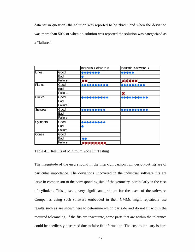
47
data set in question) the solution was reported to be “bad,” and when the deviation
was more than 50% or when no solution was reported the solution was categorized as
a “failure.”
Table 4.1. Results of Minimum Zone Fit Testing
The magnitude of the errors found in the inter-comparison cylinder output fits are of
particular importance. The deviations uncovered in the industrial software fits are
large in comparison to the corresponding size of the geometry, particularly in the case
of cylinders. This poses a very significant problem for the users of the software.
Companies using such software embedded in their CMMs might repeatedly use
results such as are shown here to determine which parts do and do not fit within the
required tolerancing. If the fits are inaccurate, some parts that are within the tolerance
could be needlessly discarded due to false fit information. The cost to industry is hard
Industrial Software A Industrial Software BLines Good
BadFailure
Planes GoodBadFailure
Circles GoodBadFailure
Spheres GoodBadFailure
Cylinders GoodBadFailure
Cones GoodBadFailure

48
to estimate due to the unknown variables (e.g. the number of CMMs using similar
software, the kinds of parts made and the fitting criterion used, etc.) but with the
amount of information shown here, potential costs even in the millions of dollars
cannot be ruled out [3,4].
4.7 Results of the Implementation
The NIST algorithm for minimum zone fitting is currently included in the ATEP test
battery. It has been tested and shown to be accurate and reliable. The algorithm will,
in the near future, be implemented in the ATEP-CMS and used for testing industrial
software.

49
5. MAXIMUM INSCRIBED AND MINIMUM CIRCUMSCRIBED FITTING
5.1 The Problem of Maximum Inscribed and Minimum Circumscribed Fitting
As well as least squares and minimum zone fitting routines, many CMS software
packages include ‘extreme’ fitting routines. Maximum inscribed and minimum
circumscribed fit routines are used in many applications. According to ANSI B89.3.1,
the maximum inscribed circle is defined as the largest circle which can be inscribed
within the measured polar profile, the minimum circumscribed circle is defined as the
smallest circle which will just contain the measured profile.
The example of a piston/cylinder assembly, such as is found in engines or automobile
fuel injectors, is commonly used to demonstrate the importance of these other fit
objectives. In the case of the piston, the maximum dimension of the outer diameter is
critical, since the piston must slide, without friction, up and down inside the cylinder.
On the other hand, the critical dimension of the cylinder is the minimum inner
diameter, since the piston must be able to move smoothly within the cylinder. The
corresponding fit objective in the case of the piston is a maximum inscribed fit,
whereas, the fit objective used for the cylinder is a minimum circumscribed fit.
The minimum circumscribed (a) and maximum inscribed (b) fits of data points for a
two- dimensional circle are shown in figure 5.1. The least squares fit routine produces
a radius of 51.411153, the minimum circumscribed fit results in a radius of

50
52.003324, and the maximum inscribed fit reports a radius of 50.871020. The data
points were created with a maximum error of 1% of the radius.
An example of points taken from the surface of a cylindrical object fit with a) a
maximum inscribed and b) a minimum circumscribed fit objective is given in figure
5.2.
Figure 5.1. Chebyshev fits for a set of circle data. The circle on the left illustrates the minimum circumscribed fit while the circle on the left illustrates the maximum inscribed fit.

51
5.2 The Need for Maximum Inscribed and Minimum Circumscribed Fitting
While the ATEP-CMS efforts have been helpful for industry, they have currently
been restricted to the problems of least squares fitting. While these are common, these
extreme fits are also needed, and they more accurately reflect some the specification
language of the American Society of Mechanical Engineers (ASME) Y14.5 and
Y14.5.1 geometric dimensioning and tolerancing standards [3], and [4]. In fact these
fits are naturally used, as applications often lend themselves to maximum-inscribed
and minimum-circumscribed fitting (e.g. cylinders and pistons, respectively.)
Figure 5.2. (a) Maximum inscribed and (b) minimum circumscribed fits for cylinder data.

52
5.3 Issues involved in solving Maximum Inscribed and Minimum Circumscribed Fitting Problems
As mentioned earlier, in the case of a circle, the minimum circumscribed and
maximum inscribed circles are based on two or three critical, extreme points. For the
other geometries (spheres and cylinders) a few more points may be required to
determine the fit. This dependence on few critical points causes these fits to be
sensitive to outliers. Bad points may drastically change the output results since the
best circle is based on only a few extreme points. Sampling patterns are also very
important in these cases; if a few extreme points on the surface of the part are not
sampled, the part may not fit as expected (say, in the case of a plug or a plug hole).
With the maximum inscribed fit it is possible for there to be more than one solution.
Figure 5.3 depicts two problematic cases. In figure 5.3(a), two circles with identical
radii are conjoined. The minimization function might choose the maximum inscribed
circle that fits either circle; while the radius is identical, the circle centers are
different. A similar problem occurs with two circles of similar size, as shown in
figure 5.3(b). In fact, the correct solution in that case would actually be the maximum
inscribed circle that fits the slightly larger circle. This special case scenario must be
dealt with somehow.

53
In the above case, and in other cases where the search space is not smooth, the global
minimum may be hidden among local minima. The minimization function must not
get trapped in these local solutions, leading to the reporting of an incorrect fit.
5.4 An approach to Maximum Inscribed and Minimum Circumscribed Fitting
5.4.1 Maximum Inscribed Circles
If time and computational energy is not an issue, a foolproof method of finding a
maximum inscribed circle fit is by way of an exhaustive search. The characteristics of
such a search are that it gives an exact result that is correct every time, it can, if
required, find multiple solutions (if they exist), it will know if a maximum inscribed
circle does in fact exist, and it will not get trapped in a local minimum that is not a
global minimum, i.e. returning an inscribed circle that is not a maximum inscribed
circle. Such a method was developed at NIST. The search is done by processing every
Figure 5.3. Two problematic geometries: (a) a surfaces with 2 equal solutions and (b) a surface with two local minimum solutions but only one true global minimum.
(a) (b)

54
3-point combination possible in the set of data points, calculating the circle formed by
the set of points, and comparing their radius to determine which one(s) are maximum
inscribed circles. This simple algorithm is effective but is also terribly inefficient. The
search uses a minimum of O(N3) operations. Analysis of data sets larger than 200
points are impractical. For this reason, the exhaustive search method is only used to
verify results from other reference algorithms produced at NIST.
The reference algorithm created to find maximum inscribed circles in an effective and
efficient manner relies on simulated annealing techniques. This method is described
in the minimum zone fit approach section. This algorithm is of the type that optimizes
a given objective function even when the global minimum is hidden among several
nearby local minima.
5.4.2 Using Simulated Annealing to Find a Maximum Inscribed Circle
The algorithm performs under the assumption that there exists at least one maximum
inscribed circle for the input data set. The program begins the search by creating an
initial guess. This is done by fitting the least squares circle to the data. The resulting
circle center is the initial guess center while the shortest distance from that center pint
to the nearest data point in the set is taken to be the initial radius. In real-life fitting
scenarios there is no problem with this choice of initial guess, while theoretical
situations may result in the odd bad fit, in reality, with CMS data this issue does not
arise.

55
The algorithm then performs a two-dimensional search to find the center of a
maximum inscribed circle (knowing the center is equivalent to knowing the solution).
The search is based on the objective function J(x) = -mini|xi-x|. Circles with centers
not inside the initial guess circle are penalized either through the simulated annealing
program or by way of a slightly expanded objective function [39].
The algorithm described above was implemented and tested at NIST against the
exhaustive search engine. The results are taken from reference above and are given
here in table 5.1.
Table 5.1. Results for simulated annealing/exhaustive search validation test.
Table 5.1a. Results from exhaustive search enginePoints Time x-center y-center Radius
100 2 100.005582854407 100.010672663295 9.90459043593364
200 20 100.000720293865 100.001376551706 9.90308030604849
400 169 100.000252864561 100.000167291954 9.90114961336861
Table 5.1b. Results using simulated annealing methodPoints Time x-center y-center Radius
100 19 100.005582854407 100.010672663295 9.90459043593364
200 35 100.000720293865 100.001376551706 9.90308030604849
400 65 100.000252864561 100.000167291954 9.90114961336861

56
While the exhaustive search was completed the search on the smaller data sets in less
time, the execution time is O(N3) compared to O(N) for the simulated annealing
method. The simulated annealed method quickly outperforms the exhaustive search
for data sets with more than 200 points (as most real-world data sets collected on
CMSs do).
The results for the two methods were identical for all 15 digits shown. Again, such a
high level of agreement with the exhaustive search solution helps validate the
simulated annealing method.
The case of a data set created with two superimposed lobed form errors (as was the
example in figure 5.3(a)) was also tested and the results further validated the
algorithm. In this case each search method found a different circle (different centers)
while the radii were identical. Further, when the radii were slightly changed, the
simulated annealing method consistently found the circle having the slightly larger
radius. This also helps to validate the simulated annealing algorithm even for these
special cases.
5.4.3 Maximum Inscribed Spheres
The case of the maximum inscribed sphere is very similar to the maximum inscribed
circle case. Though it is less often needed in practical applications, there are still
cases when it arises. The initial guess is the least squares fit sphere center with the
radius equal to the shortest distance from that center to a point in the data set.

57
The objective function for the NIST algorithms is then defined as:
)(xJR −=
Given x,
If x is inside initial guess sphere
||min)( xxxJ ii
−−=
||min2)( xxDxelseJ ii
−−=
where =D distance to initial guess sphere.
5.4.4 Other Cases of Minimum Circumscribed Fits
For minimum circumscribed circles and spheres, efficient algorithms were already in
existence. The methods already in use are both very good and any improvements that
could be made would be negligible. This method was used in the reference algorithms
for minimum circumscribed circles and spheres. More information on the method can
be found in Hopp and Reeve’s “An Algorithm for Computing the Minimum Covering
Sphere in Any Dimension” [21].
5.4.5 Maximum Inscribed and Minimum Circumscribed Fitting of Cylinders
Unlike circles and spheres, cylinders have an orientation, or direction, that must be
considered. To fit cylinders, the representation of the axis orientation must first be
dictated. For the NIST algorithms, this was done by defining a point on the axis line

58
x=(x,y,z), and by defining the direction numbers (cosines) of the axis, a=(a,b,c).
These 6 terms define the cylinder’s direction. This representation was chosen for its
straight-forwardness and simplicity. The representation could be reduced to five
numbers (using spherical coordinates) or four numbers (see [29]). However, since
speed is not a major issue in the reference algorithm creation, we are content to stick
with the 6-parameter set. A cylinder is thus defined by those 6 direction parameters
and the radius, r. This leads to the calculation of the distance of a point xi=(xi,yi,zi) to
the cylinder as di=|ax(xi-x)|, where a is A/|A|. The objective function is then created
based on these definitions. As with the previous cases, it is assumed that at least one
maximum inscribed cylinder exists and that a point on the maximum inscribed
cylinder axis lies inside the initial guess cylinder. That initial guess is again
determined using the least squares fit criteria. The best-fit cylinder direction is found
then the radius is selected in such a way that all points lie outside the resulting
cylinder.
The next step is to decide on an objective function. This was chosen to be:
Given x, A
If x is inside the initial guess,
|,,|min),( xxxzAxJ ii
−−=
||min2)( xxDxelseJ ii
−−=
Where D=distance to initial guess cylinder

59
The case of the minimum circumscribed cylinder is almost identical with the
exception of the altered objective function, which is:
Given x, A
If x is inside the initial guess,
||max),( xxAxJ ii
−=
These are the basic geometries and the approaches used to in the NIST algorithms.
More information on the above approaches can be found in [15], [16], [20], and [35]
5.5 Implementation of the Approach
The potential reference algorithms for minimum-circumscribed and maximum-
inscribed fitting (i.e. one-sided fitting) for circles, spheres, and cylinders as well as
minimum-zone fitting (i.e. two-sided fitting) for lines, planes, circles, spheres,
cylinders, and cones were extensively tested by this author. The testing consisted of
two parts: 1) testing against data specifically generated to guarantee a known,
achievable benchmark, and 2) an inter-comparison with two industrial partners using
software embedded in today's production CMSs. While this testing was designed to
help verify the NIST algorithms, additionally, alarming observations were made
about the industrial software used in the inter-comparison.
5.6 Reference vs. Commercial Algorithms for Maximum Inscribed and Minimum Circumscribed Fitting

60
As with the minimum zone fits, the maximum inscribed and minimum circumscribed
fit routines in the same two industrial software packages were tested against the NIST
reference algorithms. Data sets for circles, spheres, and cylinders were created from
the same specifications as those for the minimum zone fit routines. The results are
given in tables 5.2 and 5.3.
For the maximum-inscribed and minimum-circumscribed fits the resulting radius was
compared. The results were classified in the same manner as the minimum zone test
Table 5.3. Minimum Circumscribed Fit Results
Table 5.2. Maximum Inscribed Fit Results
Industrial Software A Industrial Software BCircles Good
BadFailure
Spheres GoodBadFailure
Cylinders GoodBadFailure
Industrial Software A Industrial Software BCircles Good
BadFailure
Spheres GoodBadFailure
Cylinders GoodBadFailure

61
results. With the exception of the Chebyshev fits for circles, the results are very
disturbing.
Some of the industry results actually gave erroneous results that were not, in fact,
minimum circumscribed or maximum inscribed fits. In several instances, the
maximum inscribed fit result circle had a number of data points that were inside the
geometry. These results are alarming. It was also found that the same problem existed
for a number of minimum circumscribed cases where data points were found to lie
outside the resultant minimum circumscribed fit circle. If these results were used by
industry, part breakdown and other more serious problems could result.
5.7 Results of the Implementation
The inter-comparison with the NIST reference algorithms brought to light some
major problems with the industrial software. Users of that software and other
packages that could be behaving similarly should be aware of these erroneous results.
While the CMS hardware might be performing well with a high level of certainty, the
software for these fit types needs to be improved and, at the least, have performance
evaluations so that users are made aware of the problems that exist.

62
6. LEAST SQUARES FITTING OF COMPLEX SURFACES
6.1 The Problem of Least Squares Fitting of Complex Surfaces
Complex surface fitting algorithms match a given point cloud to a corresponding pre-
defined surface, regardless of the surface complexity. Given an airplane wing or a
mechanical gear and a corresponding set of CMS data, be it real or virtual, the
algorithms should find the least squares fit for the surface
Figure 6.1. Two examples of complex surfaces displayed using computer graphics.

63
6.2 The Need for Fitting of Complex Surfaces
Parts such as airplane wings and fuselages, automobile doors, and satellite dishes
cannot be fit using the standard CMS software packages. The basic software packages
often have a list of basic geometric objects that can be used to model and analyze the
data sets. These basic shapes often include lines, planes, circles, spheres, cylinders,
cones, tori, and occasionally basic gear or screw shapes. More extensive algorithms
are needed to fit data to these complex surfaces.
Currently there are no standards for testing of least squares fitting software of
complex surfaces on both the national and international levels. NIST has created
reference algorithms for some general shapes to be used as a benchmark test for
industry software while, and after a standard is developed.
Some CMS software programs offer modules for measuring non-prismatic parts, such
as sheet metal and plastic assemblies, windshields, and exhaust systems, to name a
few examples. Other programs perform two- and three-dimensional best-fit routines
and contour comparisons. Such software is in the market with the ability to find least
squares approximations of complex surfaces. This is an evolving area that is
constantly expanding to include more geometries and novel new approaches to
finding a general approach to solving such problems.

64
One application of Chebyshev fitting of complex surfaces is shown in figure 6.2. The
picture represents the positioning of a cast steel part for surface machining:
Case 1 demonstrates improper positioning for machining of the part.
Case 2 shows how, by sampling the part and finding the one-sided Chebyshev fit, it
can be positioned in the optimal position for machining, so as to limit material waste
and ensure the part is machined correctly.
6.3 Issues involved in solving Least Squares Fitting of Complex Surfaces Problems
There are a number of significant problems associated with the fitting of complex
surfaces. At issue are: finding the shortest distance from the point to the surface,
fitting surfaces that are nearly translation/rotation invariant, obtaining the derivative
Figure 6.2. An application of geometric fitting of complex surfaces.

65
information (if needed for the fitting algorithm), and accurately representing arbitrary
surfaces.
The problem of finding the shortest distance from point to the surface is complicated
for multiply defined surfaces (it is hard enough for many simply defined surfaces!).
When the surface is defined by multiple geometries, it is necessary to determine
which part of the surface each point is associated with. In many cases, the shortest
distance from the point to the surface is not the correct corresponding point (as in
figure 6.3). Similarly, it can also be difficult to find the shortest distance when a point
lies near a corner or an edge. In this scenario, the point might be located at the corner
or on either side of the corner. Even for surfaces that appear to be smooth, if the
edges are segmented, each of those segments, as well as their end points, must be
tested to determine in which segment the point belongs. In the example shown in
Figure 6.3, the points located around the ‘elbow of the geometry could correspond to
either of the two line segments.
Figure 6.3. A problematic complex surface; the corner points may be mapped to either planar surface, not necessarily the correct corresponding plane.

66
A similar problem arises when there are parallel lines relatively close together. If the
collected data points are not close enough to the corresponding ‘perfect’ geometry,
confusion as to which part of the surface the point corresponds to could occur. Two
examples of this are given in Figure 6.4.
Another problem with finding the shortest distance from a point to the surface arises
in surfaces that where the distance cannot be defined by a compact expression. It is
advantageous when the problem of finding the shortest distance is a closed form
answer, that is, the solution can be found using a finite number of equations.
However, when infinite sums or iterative techniques must be implemented to obtain
the shortest distance, a sufficient number of iterations must be decided on and a ‘near
Figure 6.4. Other Problematic Complex Surfaces where the points sampled may not be mapped to the corresponding location on the surface. The shortest distance to the surface may yield an erroneous result.

67
optimal’ solution is used. This could lead to bad results if the convergence criterion is
not sufficiently high.
Also at issue are those surfaces that are nearly translation invariant or nearly rotation
invariant. Translation invariant geometries include car hood and other surfaces that
closely resemble a flat plane in one or two directions.
Part geometries can also be rotation invariant. This leads to similar problems as those
for translation invariant surfaces. Objects that vary only slightly from the shape to a
sphere, such as an egg or an apple, will rotate around one axis a lot more than the
other axes in order to get a better-fit result. In this case, a small degree of rotation
may lead to a large improvement in the fit in one-degree of rotation while rotations
along other axes may lead to relatively small improvements. It is very hard to get an
accurate result for such problems.
Another problem with complex surface least squares fit routines is that for some
solutions strategies, derivative information is needed as input to the minimization
function. In many complex surface cases, the derivative information cannot easily be
obtained. The problem is that when the function is trying to determine the distance
from a point to a surface, small changes in the x-, y-, or z- component of the surface
will lead to changes in the distance that cannot easily, or quickly, be determined.
There are a few methods of overcoming this problem. The first is to use a
minimization function that does not use derivative information. The other method is

68
to make the computer think it has the derivative information using some
approximation. This approximation can sometimes be obtained by the shortest
distance function. If the shortest distance from a point to a smooth surface is known,
the surface at the closest point can be approximated by a plane orthogonal to the
distance vector, and the derivative information associated with that plane can be used.
Lastly, it is often hard to represent, and interpret, an arbitrary surface accurately.
There are various ways to represent a surface, such as NURBS, Bezier, etc. One must
first know how to convert the given representation type to the format used by the
algorithm, if necessary. Each representation has benefits and drawbacks. Each one
must approximate the curve or surface in some way, thus some information on the
geometry is lost in each case. One solution to this problem is to look at only idealized
surfaces. One could determine to use only one mathematical formula that is good for
all 'smooth' surfaces that are not translation or rotation invariant, that is, that look
neither like a plane or a sphere. A saddle shape can be such an example.
6.4 An Approach to Solving Least Squares Fitting of Complex Surfaces Problems
In order to run, the NIST reference algorithms must be given the set of points (data
set), an initial ‘guess’ fit, the data that maps a point anywhere in the measuring
volume to the closest point on the surface, and the defining metrics for the surface
(e.g. radius, axis length, etc.).

69
Given a set of data points, a mathematically defined surface, and, in some cases, an
initial guess for the correct fit, the algorithm will find a set of ‘close points’ on the
surface through translating and rotating. These points, located on the geometry
surface, are found by determining the shortest distance from each point to the
geometry surface and selecting the point where that shortest distant vector hits the
surface as the new close point. These new points are then input as the starting points
and, again, a new set of close(r) points are found by translating and rotating. This
iterative process continues till the distance between the points and the close points
falls within the minimum distance, dictated by the input precision guidelines.
6.5 Implementation of the Approach
The testing of the NIST complex surface reference algorithms was two-fold. First,
prismatic parts were tested, and then some test cases of non-prismatic parts were used
to verify the algorithms.
6.5.1 Prismatic Parts
Prismatic surfaces were tested by comparing the algorithms’ fit solutions with the
least squares fit solution obtained from the current ATS. This ATS solution, as
previously mentioned, gives a correct fit answer using a slightly different fitting
approach. Data sets for prismatic parts, including lines, planes, circles in three

70
dimensions, spheres, cylinders, and cones were created and run through the ATS and
through the new fit algorithms.
Using the ATS, data was created for lines, circles (in two and three dimensions),
spheres, cylinders, and cones. The best fit outputs from the two algorithms were then
compared against each other, and against the ATS fits. The agreement in all of these
significantly added confidence to the results.
6.5.2 Non-Prismatic Parts
To ensure an inclusive testing regime, other surfaces, besides prismatic ones, had to
be tested. Since the current ATS does not yet have the capability to fit such surfaces,
another method for testing had to be used. The testing therefore consisted of a
comparison of the fit solutions obtained by the two independent algorithms, using the
same data set, fit file, and close points file. The creation of these ‘test data triples’ is
explained in more detail in the following paragraphs.
Data Properties:
Using Mathematica we created data for an elliptic paraboloid, hyperbolic paraboloid,
ogives, and saddle shapes. We then compared the best-fit outputs from the two
algorithms with each other. These results were used in industry as a few test cases to
evaluate software fitting performance.

71
6.5.3 Creation of Test Cases
The following parameters were used in the creation of data sets for the test cases.
1) The function that defines a rigid surface
2) A set of data points (generated by ATS2.0/mathematica)
The errors added to the data were between 1 and 2% of the defining
metric (e.g. for circle, the errors would be within 2% of the radius).
Standard surfaces (prismatic parts) created using the ATS 2.0 were
created in the following way:
The number of points were varied (between 50 and 200) also the size,
the orientation angles (azimuth & declination, where applicable), the
location of the surface within the measuring volume, and the type of
error present (for shapes created using the ATS 2.0) were changed for
each data set.
Generalized surfaces (non-prismatic parts) were created using
Mathematica in the following way:
First, the surface was defined mathematically by its function, then a set
of x, y, and z coordinates was created based on that function where

72
some random error (again between 1 and 2% of the defining metric)
was added to the z component.
3) The set of transformation data that maps each coordinate data point in the
data set to the closest point on the mathematical surface or ‘reference fit’.
Two examples follow to demonstrate how the ‘close points’ file was created. This file
was needed to determine what point on the surface each data point in the set
corresponds to. It is based on the distance of the point to the surface.
6.5.4 The ‘close points’ file for a Paraboloid
To get a fit solution from the algorithms it is necessary to have a fit and a ‘close
points’ file. The close points file is created in the following way:
First, the equation for a paraboloid is found to be 22 yxz += .
It is then necessary to find the minimum distance from a point on this surface
),,( 22 vuvu + to a point in space (p, q, r).
This is done by first finding the distance between points, as shown below:
))(()()( 22 rvuqvpuD −++−+−=
then squaring the distance results in
222222 ))(()()( rvuqvpuD −++−+−= .

73
Then it is necessary to take the partial derivatives with respect to u and v
(when the derivative = 0 you have the minimum distance), which yields:
0)2()( =−+−= rupudu
D
and
0)2()( =−+−= rvqvdv
D.
Then setting the partial derivatives equal to 0 we get:
0)21(2 223 =+−−+ qpuru
This equation was minimized in the ‘close points’ file to determine the shortest
distance and therefore the corresponding point on the surface.
6.5.5 The ‘close points’ file for a Saddle
Using the same procedure as for the paraboloid:
22 yxz +=
The function will map ),,( 22 vuvu + to (p, q, r)
Again the square of the distance is found:
2222 )()()( ruvqvpuD −+−+−=
then the the partial derivatives are found:
0)()( =−+−= ruvvpudu
D

74
0)()( =−+−= ruvuqvdv
D
Setting the derivatives equal to zero we obtain:
0)()1()2(2 222345 =+−−++−++− rqpurqpuqrupuu
Again, this equation was used in the ‘close points’ file to determine the close points
on the surface.
6.5.6 Generating Test Triples
The data sets used in testing were offset from the surface (located at the origin) by
only a slight amount. Many in industry would question the validity of such a test
regime in practice since most real-life measurement data sets would be offset a more
substantial amount from the surface in question. After the algorithms were proven to
work on point clouds located close to the surface, these data sets were translated and
rotated out to any given location and orientation within the measuring volume. The
data set that was produced with the reverse operation combined with the true fit
solution was formed and resulted in a fit solution that was very close to the correct
surface. In this way, the algorithms can be applied to any set of data points located
anywhere inside the measuring volume. This means versatility for the algorithms and
the corresponding testing measures that can be created from these algorithms.
A ‘triple’ consists of a dataset, a rigid, mathematically defined surface, and the
correct ‘least-squares fit’ solution. The first step in creating a triple is to run a surface
data set through one of the two NIST surface-fitting algorithms, generating an ATS

75
file with the translation (T2) and rotation matrix (R2) mapping the data set to the
surface. Another arbitrary translation vector (T1) and rotation matrix (R1) are created
and the original data points are moved out to this new, arbitrary, location and
orientation in space. This new set of data points is then translated and rotated by (T3)
and (R3) where T3 is the combination of T1 and T2 and R3 is the combination of R1
and R2. That is to say, the latter transformation ‘undoes’ the arbitrary
relocation/reorientation and places the data points at the correct location on the
surface. This new data set is then run through the NIST algorithm and the fit solution
is determined to be a translation of {0, 0, 0} (± 10-15) and a rotation matrix equal to
the identity matrix ± 10-15. The final triple consists of the surface in question, the
original set of data points, and the translation vector and rotation matrix that maps the
two.
These triples will eventually be made available to the public to be used in comparison
testing with their software fit algorithms.
6.5.7 Further Testing the Algorithms
The following three checks were done to validate the algorithm performance.
Check 1: Standard surface fit solution from both the algorithms were compared to the
corresponding least squares fit solution determined by the current ATS algorithms
(known to be the correct solution).

76
This testing was done on lines, planes, circles, cylinders, spheres, and cones. In all
cases the resulting fit solution had a difference from the current algorithms solution
on the order of 10-9 to 10-15. In fact, the new algorithms actually generated a better fit
(in the least squares sense) than the current ATS.
Check 2: The general surfaces least squares fit solutions were found using the
complex and quaternion algorithms. The two solutions were then compared
compared. The complex surfaces tested include paraboloids, saddles, and the surfaces
defined by xx + y, xx – yy, sin(x + y).
The data sets, the corresponding reference fits and the ‘close points’ files, were run
through these two fundamentally different algorithms and then output fit solutions
were compared. For each of the surfaces tested the solutions corresponded up to the
10-12.
Check 3:
The generalized surfaces data sets were then run through the algorithms a third time,
however this time with a ‘closecheck’ file instead of the ‘close points’ file. The
‘closecheck’ file finds the closest point on the surface using the Mathematica function
‘FindMinimum’ to obtain the close points on the surface. In all cases the results were
within 10-12 of the previously found fit solutions.

77
Check 4: The general surface fit solutions (found in ‘check 2’) were then used to
create test data triples (as described above) to move the surface to some arbitrary
location in space then translate and rotate it back to the surface, using the fit result
numbers to ensure that correct translation and rotation matrices are being produced by
the algorithms.
The re-oriented data sets were then run through the algorithms in the same way the
original data had been. The solutions were within 10-10 of the correct solution of {0,
0, 0}, I. Where the zero vector is the translation (the new (x, y, z) value) and the
rotation is he identity matrix (meaning the data was not moved from its start position
in order to obtain the correct fit).
6.6 Results of the Implementation
The result was that, in all cases, the fit solution for the complex least squares
algorithm matched the results obtained using the original least squares fitting
algorithms for standard shapes.
The algorithms proved reliable for repeated runs with differing data sets. The function
written to find the distance from the points to the surface (different for each different
geometry) were also varied. Both the original function and a function using the
Mathematica function 'FindMinimum' were used and compared against each other.
The results, in these cases, were identical. The conclusion was that the algorithms
work well.

78
NIST's algorithms for least squares fitting of complex surfaces were tested under a
wide range of test scenarios. The results of the testing showed that the algorithms
performed well. A possible source of error is the function that must be created to find
the distance from the points to the surface. If this function is written incorrectly the
minimization function will give bad results. By checking the results against the same
data set run with the ‘FindMinimum’ function any errors should be evident in the
differing fit results.
7. OTHER ISSUES AND FUTURE WORK
7.1 Other Issues Involved in CMS Fitting Software
There are some differences between the work going on in other parts of the world and
this work. Questions arise as to what basic test generation techniques should be used.
One such question involves the generation of reference results. As mentioned in
section 2.3, some feel it is better to generate solutions from data sets rather than
having an independent reference algorithm to generate the reference solutions. Doing
so reduces the work by eliminating the reference algorithm generation. There are
however, serious drawbacks to such an approach. Firstly, the amount of time and
effort saved is limited. Once the volume of data sets you must find results for gets too
big or too complicated it might take more time to go through the process of finding a
solution to each data set rather than having the generic solution that you can just run

79
the data sets through to get your solution. Another problem is that when data sets are
too small or have a poor sampling area, there may not be a single unique solution. In
this case software might be performing correctly by not agreeing with the reference
solution.
The choice of a sampling strategy was touched on briefly, however the issue is much
broader than what has been described. According to Bosh, “Some sampling strategies
can greatly amplify the error introduced at each measurement point, while other
sampling strategies can reduce the error. …Since the CMM user selects the sampling
strategy, different measurement results, and these results may have very different
uncertainties associated with them.” [6]. Bosh later writes that, “The sampling
strategy issue is one of the factors which makes the evaluation of CMM measurement
uncertainty difficult. Even if the uncertainty due to the form error of the part is known
exactly, the uncertainty of the measurement result, e.g., the diameter of a circle is
unknown until a particular sampling strategy is specified for the measurement.” [6].
7.2 Future Work
Currently the ATS is limited to reference algorithms for least-squares fitting of
standard parts. Due to interest from the industrial sector, NIST is extending the
capabilities of the ATS to allow for other fit types including minimum inscribed,
maximum circumscribed, and minimum zone fits for relevant features. Also, the least
squares fit routines are being extended to include fits for non-standard features such
as those mentioned in the previous pages. These fit routines have been developed in a

80
way that reflects the standards for CMS software performance currently being
developed on both the national and international levels.
Further expansion of the ATS is already being planned. Future projects include the
creation of reference algorithms for least squares fitting of patchwork surfaces
including geometries generated by CAD software. The test service will also include
reference algorithms for a wide variety of complex surfaces in the least squares fit
category.
Also, the current algorithms that fit data sets to data clouds have been developed as
part of the least squares fitting algorithms for complex surfaces and will be
implemented in the ATEP as needed. As the industry expands so too does the work
done on the same fitting problems at NIST.
A web-based ATEP will be completed in the near future. Features of the web site
include background information on various fit types and common problems
encountered with CMS software and a listing of related references. Reference data
sets will be available for download along with the corresponding reference fits
generated by the NIST reference algorithms. Users will then be able to perform
independent checks of their software. Contact information will also be given for the
times when a more specialized or thorough test service is desired, or if certification is
required. Such a service will be of great benefit to many throughout industry.

81
8. Conclusions
This thesis is written with two primary goals. The first goal is to be a repository of
information related to CMS software uncertainty and fitting algorithms that can be
referenced by industry. The second goal is to give an overview of the work the author
has contributed on reference algorithm testing done at NIST and the results of that
work. Those results point to major problems with CMS software currently in use in
industry today. A summary of the application of least squares fitting and the findings
of the reference algorithm testing follows.
A least squares fitting application was overviewed in chapter 3. A reference algorithm
was generated to test industry software that has been created for use in a non-
destructive ultrasonic spot-weld detector. The reference algorithm was created to be
extremely precise and reliable, rather than fast and easy-to-use. This application is an
example of one of the many uses of least squares fitting routines and the way in
which testing may be carried out using a reference algorithm. The result of the
reference algorithm testing (the inter-comparison done with against the industry
software) was that the industry software was correct to two decimal places (the spot
weld detector only displayed results up to a maximum of three decimal places). For
the purposes of the spot-weld detector application this is sufficient accuracy. For this
reason, the software was determined to be performing well as evidenced by the NIST
reference algorithm inter-comparison.

82
The NIST minimum zone reference algorithms were developed based on the
phenomenon of simulated annealing (SA). Testing of the algorithms for minimum
zone fits involved creating data sets with known solutions then running the data
through the reference algorithms to ensure that they gave the correct (known) answer.
For all geometries tested (lines, planes, circles (2- and 3-D), cylinders, spheres, and
cones) and for all sizes, location, and orientation of those geometries, the reference
algorithms were found to give the correct fit result up to 15 decimal places (more if
the minimization function was set to have a more rigid convergence criterion). This
verified that the reference algorithms for minimum zone fits are accurate and reliable.
Two inter-comparisons were run using the NIST algorithms for minimum zone fits as
a reference. The two industrial software packages processed the reference data sets
for lines, planes, circles, spheres, cylinders, and, for the first software package, cones.
For first software package, two out of ten data sets for lines failed with deviation from
the NIST ‘correct fit result’ at more than 50%. The cones performed even more
poorly, with eight of the ten data sets failing to come within 50% agreement with
NIST results. For lines, cylinders, and cones, the first industrial software package
tested had additional one, one, and two data sets respectively that were only within 10
and 50% agreement with the NIST results. The second inter-comparison partner did
not fair much better with five of the ten data sets for lines and one of the ten data sets
for planes failing to agree within 50% of the reference results. In these cases, the
results did not in any way match the true results. This points to serious problems with

83
the industrial software packages tested. While only two packages were used for inter-
comparison, the results indicate that substantial problems exist in both packages.
The reference algorithms for one-sided Chebyshev fits (maximum inscribed and
minimum circumscribed) were also developed based on the principle of simulated
annealing. The maximum inscribed and minimum circumscribed reference algorithm
testing consisted of two parts: 1) testing against data specifically generated to
guarantee a known achievable benchmark, and 2) an inter-comparison with two
industrial partners using software embedded in today's production CMSs.
The simulated annealing algorithm, together with the minimum zone objective
function was used to determine the geometry that minimized the maximum
magnitude of the two extreme residuals (one on either ‘side’ of the resulting
geometry). The algorithms were tested and found to work very well.
In the case of the maximum inscribed fit routines, the first inter-comparison partner,
the results for one of the ten data sets for spheres gave failing results, with agreement
with the NIST results less than 50%. And failing results for five of the nine cylinder
data sets, as well as one ‘bad’ cylinder data fit with agreement between 10% and 50%
with the NIST fit results. The second industrial software package yielded one bad
circle fit result, out of ten test data sets, and one bad cylinder fit result, out of ten test
cases. The sphere cases were extremely poor, with all ten data sets tested giving
incorrect results that did not agree within 50% of the NIST reference results.

84
The minimum circumscribed fit routines did not perform much better. The first
software package tested resulted in failure for one of seven sphere data sets and five
of nine cylinder data sets. It also gave ‘bad’ results (within 1- and 50% agreement
with the NIST reference result) for one of the nine cylinder data sets. The second
software package gave good (within 10% agreement with NIST results) fit results for
all circle and cylinder data sets tested, however nine of the ten data sets for spheres
gave failing results.
Also, some of the industry results actually gave erroneous results that were not, in
fact, maximum inscribed or minimum circumscribed fits.
The NIST reference algorithms for least squares fitting of complex surfaces were also
tested to ensure a high level of performance. The testing of these algorithms involved
testing of both standard (prismatic) and general (non-prismatic) surfaces. Prismatic
surfaces were tested by comparing the complex surface reference algorithms’ fit
solutions to the corresponding least squares fit solution obtained from the ATS. In
this way, data sets for prismatic parts, including lines, planes, circles (3D), spheres,
cylinders, and cones were created and run through the ATS and through the least
squares fitting algorithms for complex surfaces. This reference testing was done on
lines, planes, circles, cylinders, spheres, and cones. In all cases the resulting fit
solution found using the complex surface fitting algorithms had differences (from the
ATS solution) on the order of 10-9 to 10-15. In fact, the new algorithms actually

85
generated a better fit (in the least squares sense) than the current ATS. This validated
the reference algorithms for the cases of these standard surfaces.
Numerous test cases were then created for complex surfaces, including paraboloids,
saddles, sine functions, and other non-standard surfaces. These triples consist of the
mathematical function that defines the surface, a set of data points corresponding to
that surface with random error added between 1 to 2% of the defining metric, and the
set of transformation data that maps each coordinate data point in the data set to the
closest point on the mathematical surface or ‘reference fit’. The general surfaces least
squares fit solutions were found using both the complex and quaternion algorithms
(two reference algorithms created to perform the same task in different ways). The
two resulting solutions were then compared to each other. The complex surfaces that
were tested include paraboloids, saddles, and the surfaces defined by xx + y, xx – yy,
sin (x + y). For each of the surfaces tested the solutions corresponded up to the 10-12.
This validated the performance of the NIST reference algorithms for these complex
surfaces.
These test cases, along with the resultant reference solutions will be used to form test
triples, consisting of a data set, a rigid, mathematically defined surface, and the
correct ‘least-squares fit’ solution as determined by the reference algorithms. These
will serve industry as a self-check mechanism available for download at some point
in the future.

86
The testing of the NIST algorithms in the ways described above confirms the validity
and high degree of accuracy of the reference algorithms. The test regime
demonstrated that the NIST algorithms are reliable and can be used as a reference
against which to test industry software. Such a testing tool is very valuable to
industry.
The results of the industry inter-comparisons done so far indicate that there are major
trouble areas in the industry algorithms for Chebyshev fit objectives. While the least
squares fit results for standard surfaces appear to do well, the minimum-zone fit
results for lines, as well as the minimum circumscribed and maximum inscribed fits
for spheres were proven to be performing poorly. The magnitude of the errors found
in the inter-comparison output fits is of particular importance. The inconsistencies
found in the industrial partner software fits are very large in relation to the geometric
size of the surface. Also, some maximum inscribed fits were not really inscribed at
all, and the same with some minimum circumscribed fits. This indicates a significant
problem for the users of the software. With the errors evident in these inter-
comparison results, millions of dollars of parts may be discarded annually due to
these erroneous results. Depending on the number of CMSs currently using these
software packages, and others with similar problems, the parts being needless wasted
could be on the order of millions, or even tens of millions. These particular fit
routines, and others like it, must be improved in order to protect the users from such a
large financial loss.

87
REFERENCES
[1] Agin, G.J., Fitting Elipses and General Second-Order Curves, Carnegi-Mellon University, Robotics Institute, Technical Report 81-5, (1981).
[2] Ahn, S.J., et al. Least-Squares Orthogonal Distances Fitting of Circle, Sphere, Ellipse, Hyperbola, Pattern Recog. 34, (2001), 2283-2303.
[3] ASME, Dimensioning and Tolerancing, ANSI/ASME Y14.5, American Society of Mechanical Engineers, New York City, and American National Standards Institute, New York City, (1994).
[4] ASME, Mathematical Definitions of Dimensioning and Tolerancing, ANSI/ASME Y14.5.1, American Society of Mechanical Engineers, New York City, and American National Standards Institute, New York City, (1994).
[5] ASME, Methods for Performance Evaluation of Coordinate Measuring System Software, ASME B89.4.10–2000, American Society of Mechanical Engineers, New York City, (2002).
[6] Bosch, John. Coordinate Measuring Machines and Systems, Marcel Dekker Inc., New York, (1995).
[7] Chernov, N.I. and G.A. Ososkov, Effective Algorithms for Circle Fitting, Comp. Phys. Comm. 33, (1984), 329-333.
[8] Chojnacki, W., et al. Raltionalising the Renormalization Method of Kanatani, J. Math. Imaging & Vision 14, (2001), 21-38.
[9] Cox, M.G., and P.M. Harris. The Design and Use of Reference Data Sets for Testing Scientific Software, National Physical Laboratory, Teddington, Middlesex UK, (1998).
[10] Cox, M.G., et al.,Validation of CMM Form and Tolerance Assessment Software. National Physical Laboratory, Teddington, Middlesex UK, (2001).

88
[11] Diaz, Cathleen and Theodore Hopp, “Testing of Coordinate Measuring System Software”, Proceedings of the 1993 American Society for Quality Control Measurement Quality Conference, (1993).
[12] Diaz, C, “Algorithm Testing and Evaluation Program for Coordinate Measuring Systems: Testing Methods”, National Institute of Standards and Technology, NISTIR 5686 (1995).
[13] Diaz, C, “Concept for an Algorithm Testing and Evaluation Program at NIST”, Natl. Inst. Stand. Technol., NISTIR 5366, (1994).
[14] Diaz, C., and T. Hopp, “Evaluation of Software for Coordinate Measuring Systems”, Proc. (1995) SME Clinic, CMMs Week, June 5–8, Soc. of Manuf. Eng., Dearborn, MI; also in Proc. 1995 Interface Symp., June 21–24, Interface Foundation of North America, Carnegie Mellon Univ., Pittsburgh, PA (June 1995).
[15] Diaz, C., and T. Hopp, “Testing Coordinate Measuring Systems Software”, Proc. 1994 Natl. Conf. Stand. Lab. Ann. Workshop and Symposium (Aug. 1994).
[16] Duncan, Christian, et al., “Efficient Approximation and Optimization Algorithms for Computational Metrology”, SODA: ACM-SIAM, (1997).
[17] Gander, W. and U. von Matt, Some Least Squares Problems, Solving Problems in Scientific Computing Using Maple and Matlab, 251-266, Springer-Verlag, (1993).
[18] Hogan, Michael, et al., “Information Technology Measurement and Testing Activities at NIST” J. Res. Natl. Inst. Stand. Technol. 106, 341-370 (2001).
[19] Hopp, T.H. “Computational Metrology”, Manufacturing Review 6 (4), 295–304, ASME, NY (1993), 295-304.

89
[20] Hopp, Theodore, and Mark Levenson. “Performance Measures for Geometric Fitting in the NIST Algorithm Testing and Evaluation Program for Coordinate Measurement Systems.” J. Res. Natl. Inst. Stand. Technology. 100 (5), 563-574, (1995).
[21] Hopp, Theodore, and Charles Reeve. An Algorithm for Computing the Minimum Covering Sphere in Any Dimension. National Institute of Standards and Technology, NISTIR 5831, (1996).
[22] ISO, Guide to the Expression of Uncertainty in Measurement, International Organization for Standardization, Geneva, Switzerland (1993).
[23] ISO 10360-3:2000 International Organization for Standardization, Geneva Switzerland, (2000)
[24] ISO 15530 International Organization for Standardization, Geneva Switzerland (1994)
[25] Kasa, I., A Curve Fitting Procedure and its Error Analysis, IEEE Tans. Inst. Meas. 25, (1976), 8-14.
[26] Lawson C.L., and R.J. Hanson, Solving Least-Squares Problems, Prentice-Hall, (1974).
[27] Linnik, Vladimirovich Y. Method of Least Squares and Principles of the Theoryof Observations, New York, Pergamon Press, (1961).
[28] Marquardt, D., An algorithm for Least Squares Estimation of Nonlinear Parameters, SIAM J. Appl. Math. 11, (1963), 431-441.
[29] Matthews, James, (2000), http://www.generation5.org/content/2000/anneal.aspJune 22, 2003.
[30] Moura, L. and R.I. Kitney, A Direct Method for Least-Squares Circle Fitting, Comp. Phys. Comm. 64, (1991), 57-63.

90
[31] Nelder J.A., and R. Mead. “A Simplex Method for Function Minimization”, Computer Journal, 7:308-313, (1965).
[32] Pearson, C., Numerical Methods in Engineering and Science, Van Nostrand Reinhold, (1986).
[33] Powell, M. J. D., “An Efficient Method for Finding the Minimum of a Function of Several Variables without Calculating Derivatives”, Computer Journal, 7, (1964), 152-162.
[34] Pratt, V. Direct Least-Squares Fitting of Algebraic Surfaces, Computer Graphics21, (1987), 145-152.
[35] Press, William H. et al., Numerical Recipes in C;|The Art of Scientific Computing, 2nd Ed. Cambridge University Press, New York, (1992).
[36] Rayner, Dave, and Maurice Cox. National Measurement System: Software Support for Metrology Programme. National Physical Laboratory, Teddington, Middlesex UK, (April 2001).
[37] Robinson, S.M., Fitting Spheres by the Method of Least Squares, Commun. Assoc. Comput. Mach. 4, (1961), 491.
[38] Sampson, P.D., Fitting Conic Sections to Very Scattered Data: an Iterative Refinement of the Bookstein Algorithm, Comp. Graphics Image Proc. 18, (1982), 97-108.
[39] Shakarji, C.M., “Least-squares Fitting Algorithms of the NIST Algorithm Testing System”, J. Res. Natl. Inst. Stand. Technology. 103 (6), 633-641.
[40] Shakarji, Craig, and John Raffaldi, Should You be Concerned With Software Measurement Uncertainty? Proceedings of the International Dimensional Workshop 2003, Nashville, (2003).
[41] Spath, H. Least Squares Fitting By Circles, Computing 57, (1996), 179-185.

91
[42] Sym, Roger. An Assessment of the Extent to which Metrology Algorithms are Used in Standards. (July 19, 2002).
[43] Taylor, B.N., and C.E. Kuyatt, “Guidelines for Evaluating and Expressing the Uncertainty of NIST Measurement Results”, NIST Technical Note 1297, National Institute of Standards and Technology, Gaithersburg, MD (1994).
[44] Walker, R., GIDEP Alert X1-A-88-01, CMM Form Tolerance Algorithm Testing, Government-Industry Data Exchange Program, DOD, Washington, D.C., (1988).
[45] Wichmann, Brian., Software Support for Metrology Best Practice Guide No. 1: Measurement System Validation: Validation of Measurement Software NPL, Middlesex, UK, (April 2000).
[46] Wismer, D.A., and R. Chattergy, Introduction to Nonlinear Optimization. System science and engineering, North-Holland, (1978).