ABSTRACT

Title of dissertation: SATELLITE NETWORKDESIGN, OPTIMIZATIONAND MANAGEMENT

Ioannis Gamvros, Doctor of Philosophy, 2006

Dissertation directed by: Professor Subramanian RaghavanRobert H. Smith School of Business

We introduce several network design and planning problems that arise in the

context of commercial satellite networks. At the heart of most of these problems

we deal with a traffic routing problem over an extended planning horizon. In satel-

lite networks route changes are associated with significant monetary penalties that

are usually in the form of discounts (up to 40%) offered by the satellite provider

to the customer that is affected. The notion of these rerouting penalties requires

the network planners to consider management problems over multiple time periods

and introduces novel challenges that have not been considered previously in the

literature.

Specifically, we introduce a multiperiod traffic routing problem and a multi-

period network design problem that incorporate rerouting penalties. For both of

these problems we present novel path-based reformulations and develop branch-

and-price-and-cut approaches to solve them. The pricing problems in both cases

present new challenges and we develop special purpose approaches that can deal

with them. We also show how these results can be extended to deal with traf-

fic routing and network design decisions in other settings with much more general

rerouting penalties. Our computational work demonstrates the benefits of using the

branch-and-price-and-cut procedure developed that can deal with the multiperiod

nature of the problem as opposed to straightforward, myopic period-by-period op-

timization approaches.

In order to deal with cases in which future demand is not known with certainty

we present the stochastic version of the multiperiod traffic routing problem and

formulate it as a stochastic multistage recourse problem with integer variables at

all stages. We demonstrate how an appropriate path-based reformulation and an

associated branch-and-price-and-cut approach can solve this problem and other more

general multistage stochastic integer multicommodity flow problems.

Finally, we motivate the notion of reload costs that refer to variable (i.e.,

per unit of flow) costs for the usage of pairs of edges, as opposed to single edges.

We highlight the practical and theoretical significance of these cost structures and

present two extended graphs that allow us to easily capture these costs and generate

strong formulations.

SATELLITE NETWORK DESIGN, OPTIMIZATION ANDMANAGEMENT

by

Ioannis Gamvros

Dissertation submitted to the Faculty of the Graduate School of theUniversity of Maryland, College Park in partial fulfillment

of the requirements for the degree ofDoctor of Philosophy

2006

Advisory Committee:

Professor Subramanian Raghavan, Chair/AdvisorProfessor Steve GabrielProfessor Bruce GoldenProfessor Itir KaraesmenProfessor Hani Mahmassani

c© Copyright by

Ioannis Gamvros

2006

IJAKH

Sa bgeÐc ston phgaimì gia thn Ij�kh,na eÔqesai na eÐnai makrÔc o drìmoc,gem�toc peripèteiec, gem�toc gn¸seic.

Touc Laistrugìnac kai touc KÔklwpac,ton jumwmèno Poseid¸na mh fob�sai,

tètoia ston drìmo sou potè sou den ja breÐc,an mèn` h skèyic sou uyhl , an eklekt 

sugkÐnhsic to pneÔma kai to s¸ma sou aggÐzei.Touc Laistrugìnac kai touc KÔklwpac,ton �grio Poseid¸na den ja sunant seic,an den touc koubaneÐc mec thn yuq  sou,

an h yuq  sou den touc st nei emprìc sou.

Na eÔqesai n�nai makrÔc o drìmoc.Poll� ta kalokairin� prwin� na eÐnai

pou me ti euqarÐsthsi, me ti qar�ja mpaÐneic se limènac prwtoeidwmènouc;na stamat seic s` emporeÐa Foinikik�,

kai tec kalèc pragm�teiec n` apokt seic,sentèfia kai kor�llia, keqrimp�ria k` èbenouc,

kai hdonik� murwdik� k�je log c,ìso mporeÐc pio �fjona hdonik� murwdik�;

se pìleic Aiguptiakèc pollèc na pac,na m�jeic kai na m�jeic ap` touc spoudasmènouc.

P�nta ston nou sou n�qeic thn Ij�kh.To fj�simon ekeÐ eÐn` o proorismìc sou.

All� mhn bi�zeic to taxÐdi diìlou.KallÐtera qrìnia poll� na diarkèsei;

kai gèroc pia n` ar�xeic sto nhsÐ,ploÔsioc me ìsa kèrdisec ston drìmo,

mh prosdok¸ntac ploÔth na se d¸sei h Ij�kh.

H Ij�kh s` èdwse to wraÐo taxÐdi.QwrÐc aut n den j�bgainec ston drìmo.

'Alla den èqei na se d¸sei pia.

Ki an ptwqik  thn breÐc, h Ij�kh den se gèlase.'Etsi sofìc pou èginec, me tìsh peÐra,

 dh ja to kat�labec oi Ij�kec ti shmaÐnoun.

KwnstantÐnoc P. Kab�fhc (1911)

ii

ITHAKA

When you set out on your journey to Ithaca,pray that the road is long,

full of adventure, full of knowledge.The Lestrygonians and the Cyclops,

the angry Poseidon – do not fear them;You will never find such as these on your path,

if your thoughts remain lofty, if a fineemotion touches your spirit and your body.

The Lestrygonians and the Cyclops,the fierce Poseidon you will never encounter,if you do not carry them within your soul,

if your soul does not set them up before you.

Pray that the road is long.That the summer mornings are many, when,

with such pleasure, with such joyyou will enter ports seen for the first time;

stop at Phoenician markets,and purchase fine merchandise,

mother-of-pearl and coral, amber and ebony,and sensual perfumes of all kinds,

as many sensual perfumes as you can;visit many Egyptian cities,

to learn and learn from scholars.

Always keep Ithaca in your mind.To arrive there is your ultimate goal.But do not hurry the voyage at all.

It is better to let it last for many years;and to anchor at the island when you are old,

rich with all you have gained on the way,not expecting that Ithaca will offer you riches.

Ithaca has given you the beautiful voyage.Without her you would have never set out on the road.

She has nothing more to give you.

And if you find her poor, Ithaca has not deceived you.Wise as you have become, with so much experience,

you must already have understood what Ithacas mean.

Constantine P. Cavafy (1911)

iii

DEDICATION

To my parents and Gianni, Rena, Anesti, and Katerina.

iv

ACKNOWLEDGMENTS

First and foremost I would like to thank my advisor, Professor S. Raghavan, for

his guidance and support throughout all my years at the University of Maryland. His

course on Network Planning and Design was one of the first courses that I attended

as a student in College Park and was what sparked my interest in Management

Science. Moreover, he has always made himself available for advice and direction

and provided numerous solutions both to my research problems and otherwise. Our

very fruitful and easygoing cooperation made my time as a Ph.D. student a very

pleasant experience. Additionally, his help and advice while I was looking for a job

was invaluable.

I would also like to thank, Professor Bruce Golden who invited me to join the

Ph.D. program in the Robert H. Smith School of Business back in the fall of 2002.

It seems surprising to me now that back then he and Dr. Raghavan actually had

to make a considerable effort in convincing me to join the program. Initially I was

very reluctant in joining the Ph.D. program but now I really cannot imagine where

I would be without the tools and know-how I have gathered during my time at the

business school. I also greatly appreciate, Dr. Golden’s significant assistance with

my early research and this dissertation as well as my search for a job at the end of

the Ph.D. program.

Thanks are also due to Professors Itir Karaesmen, Steven Gabriel and Hani

v

Mahmassani for agreeing to serve on my thesis committee and for sparing consid-

erable time reviewing the manuscript. Based on their input, comments and sugges-

tions I discus several additional issues in this thesis which have greatly improved

the quality of the text.

Additionally, I would also like to thank Hany Eldeib, Bruno Fromont and

Bellur Srikar from Intelsat Global Service Corporation for giving me the opportunity

to work at Intelsat. Their support, especially during my first internship at Intelsat,

in the summer of 2003 when I was still a very inexperienced MS professional is

greatly appreciated. Our continual cooperation through 2004 and 2005 provided the

motivation, technical details and managerial insights that made this thesis possible.

Finally, I owe my deepest gratitude to my family, my mother and father, who

have been a continual source of strength and support throughout my graduate years.

vi

Contents

List of Tables ix

List of Figures xii

1 Introduction 11.1 A Brief History of the Satellite Industry . . . . . . . . . . . . . . . . 11.2 The Current Commercial Satellite Communications Market . . . . . . 51.3 A Brief Technical Overview of Satellite Communications . . . . . . . 91.4 Satellite Network Management and Operational Problems . . . . . . 111.5 Outline of the Dissertation . . . . . . . . . . . . . . . . . . . . . . . . 16

2 Multiperiod Traffic Routing 192.1 Problem Definition . . . . . . . . . . . . . . . . . . . . . . . . . . . . 192.2 Related Literature . . . . . . . . . . . . . . . . . . . . . . . . . . . . 202.3 Problem Formulation . . . . . . . . . . . . . . . . . . . . . . . . . . . 222.4 Solution Approach . . . . . . . . . . . . . . . . . . . . . . . . . . . . 26

2.4.1 Overview . . . . . . . . . . . . . . . . . . . . . . . . . . . . . 262.4.2 Pricing . . . . . . . . . . . . . . . . . . . . . . . . . . . . . . . 292.4.3 Cutting . . . . . . . . . . . . . . . . . . . . . . . . . . . . . . 392.4.4 Other Considerations . . . . . . . . . . . . . . . . . . . . . . . 42

2.5 Computational Results . . . . . . . . . . . . . . . . . . . . . . . . . . 462.5.1 Multiperiod vs. Period-by-Period . . . . . . . . . . . . . . . . 492.5.2 BPC vs. Root-Node . . . . . . . . . . . . . . . . . . . . . . . 562.5.3 Real-world Instances . . . . . . . . . . . . . . . . . . . . . . . 60

2.6 Concluding Remarks . . . . . . . . . . . . . . . . . . . . . . . . . . . 61

3 Traffic Routing with Onboard Configuration Decisions 643.1 Problem Definition . . . . . . . . . . . . . . . . . . . . . . . . . . . . 643.2 Related Literature . . . . . . . . . . . . . . . . . . . . . . . . . . . . 653.3 Problem Formulation . . . . . . . . . . . . . . . . . . . . . . . . . . . 663.4 Solution Approach . . . . . . . . . . . . . . . . . . . . . . . . . . . . 69

3.4.1 Pricing and General Penalties . . . . . . . . . . . . . . . . . . 693.4.2 Other Considerations . . . . . . . . . . . . . . . . . . . . . . . 733.4.3 Linear Configuration Variables . . . . . . . . . . . . . . . . . . 75

3.5 Computational Results . . . . . . . . . . . . . . . . . . . . . . . . . . 773.5.1 Multiperiod vs. Period-by-Period . . . . . . . . . . . . . . . . 783.5.2 BPC vs. Root-Node . . . . . . . . . . . . . . . . . . . . . . . 863.5.3 Integer vs. Linear Configuration Variables . . . . . . . . . . . 91

3.6 Concluding Remarks . . . . . . . . . . . . . . . . . . . . . . . . . . . 93

4 Multiperiod Traffic Routing with Uncertain Demand 954.1 Problem Definition . . . . . . . . . . . . . . . . . . . . . . . . . . . . 954.2 Related Literature . . . . . . . . . . . . . . . . . . . . . . . . . . . . 964.3 Problem Formulations . . . . . . . . . . . . . . . . . . . . . . . . . . 100

vii

4.3.1 Uncertainty . . . . . . . . . . . . . . . . . . . . . . . . . . . . 1004.3.2 Flow Based Model . . . . . . . . . . . . . . . . . . . . . . . . 1034.3.3 Path Based Model . . . . . . . . . . . . . . . . . . . . . . . . 105

4.4 Solution Approach . . . . . . . . . . . . . . . . . . . . . . . . . . . . 1074.4.1 L-Shaped Algorithm . . . . . . . . . . . . . . . . . . . . . . . 1084.4.2 Master Problem, Feasibility and Optimality Cuts . . . . . . . 1114.4.3 Branch-and-Price . . . . . . . . . . . . . . . . . . . . . . . . . 115

4.5 Stochastic Multistage Multicommodity Flow Integer Recourse . . . . 1174.6 A Note On Robust Optimization . . . . . . . . . . . . . . . . . . . . 1234.7 Computational Results . . . . . . . . . . . . . . . . . . . . . . . . . . 126

4.7.1 Expected Value Solutions . . . . . . . . . . . . . . . . . . . . 1274.7.2 Wait-and-See Solutions . . . . . . . . . . . . . . . . . . . . . . 1294.7.3 General Problem Characteristics . . . . . . . . . . . . . . . . . 1294.7.4 Stochastic vs. Expected . . . . . . . . . . . . . . . . . . . . . 1334.7.5 Stochastic vs. Wait-and-See . . . . . . . . . . . . . . . . . . . 1364.7.6 Random Scenario Generation . . . . . . . . . . . . . . . . . . 136

4.8 Concluding Remarks . . . . . . . . . . . . . . . . . . . . . . . . . . . 139

5 VPN Design in Satellite Networks - Reload Cost Trees 1415.1 Problem Definition . . . . . . . . . . . . . . . . . . . . . . . . . . . . 1415.2 Related Literature . . . . . . . . . . . . . . . . . . . . . . . . . . . . 1425.3 Problem Formulations . . . . . . . . . . . . . . . . . . . . . . . . . . 146

5.3.1 Directed Formulation . . . . . . . . . . . . . . . . . . . . . . . 1485.3.2 Line Graph Formulation . . . . . . . . . . . . . . . . . . . . . 1505.3.3 Node-Color Graph Formulation . . . . . . . . . . . . . . . . . 156

5.4 Reload Cost Problems - Extensions . . . . . . . . . . . . . . . . . . . 1625.4.1 Routing Costs . . . . . . . . . . . . . . . . . . . . . . . . . . . 1625.4.2 Tree Network Design . . . . . . . . . . . . . . . . . . . . . . . 1635.4.3 Uncapacitated Network Design . . . . . . . . . . . . . . . . . 164

5.5 Computational Results . . . . . . . . . . . . . . . . . . . . . . . . . . 1665.5.1 Forcing Constraints . . . . . . . . . . . . . . . . . . . . . . . . 1675.5.2 Comparison of LGFB vs. CGFB . . . . . . . . . . . . . . . . 169

5.6 Concluding Remarks . . . . . . . . . . . . . . . . . . . . . . . . . . . 172

6 Summary, Contributions, and Concluding Remarks 1766.1 Summary . . . . . . . . . . . . . . . . . . . . . . . . . . . . . . . . . 1766.2 Further Research and Application Opportunities . . . . . . . . . . . . 187

viii

List of Tables

1.1 Comparison of technical characteristics between a fiber optic cablesystem and a GEO satellite system (Gbps = Gigabits per second,Tbps = Terabits per second, ms = milliseconds). . . . . . . . . . . . . 8

2.1 Problem parameters used in the random problem generation. . . . . . 48

2.2 Comparison of Period-by-Period to Multiperiod optimization for dif-ferent load-factors. . . . . . . . . . . . . . . . . . . . . . . . . . . . . 54

2.3 Comparison of Period-by-Period to Multiperiod optimization for dif-ferent rerouting penalty values. . . . . . . . . . . . . . . . . . . . . . 54

2.4 Comparison of Period-by-Period to Multiperiod optimization for dif-ferent time periods. . . . . . . . . . . . . . . . . . . . . . . . . . . . . 55

2.5 Comparison of Period-by-Period to Multiperiod optimization for dif-ferent numbers of customers (commodities). . . . . . . . . . . . . . . 55

2.6 Comparison of the Root-Node approach to the BPC procedure forlow variance demand. . . . . . . . . . . . . . . . . . . . . . . . . . . . 58

2.7 Comparison of the Root-Node approach to the BPC procedure forhigh variance demand. . . . . . . . . . . . . . . . . . . . . . . . . . . 58

2.8 Comparison of the Root-Node approach to the BPC procedure forhigh variance demand and increased number of customers. . . . . . . 59

3.1 Problem parameters used in the random problem generation for bothdata sets. . . . . . . . . . . . . . . . . . . . . . . . . . . . . . . . . . 79

3.2 Comparison of Period-by-Period to Multiperiod optimization underdifferent load-factors for single-configuration satellites in the first dataset. . . . . . . . . . . . . . . . . . . . . . . . . . . . . . . . . . . . . . 83

3.3 Comparison of Period-by-Period to Multiperiod optimization underdifferent load-factors for satellites with two configurations in the firstdata set. . . . . . . . . . . . . . . . . . . . . . . . . . . . . . . . . . . 83

3.4 Comparison of Period-by-Period to Multiperiod optimization underdifferent load-factors for satellites with three configurations in thefirst data set. . . . . . . . . . . . . . . . . . . . . . . . . . . . . . . . 84

ix

3.5 Comparison of Period-by-Period to Multiperiod optimization underdifferent load-factors for single-configuration satellites in the seconddata set. . . . . . . . . . . . . . . . . . . . . . . . . . . . . . . . . . . 84

3.6 Comparison of Period-by-Period to Multiperiod optimization underdifferent load-factors for satellites with two configurations in the sec-ond data set. . . . . . . . . . . . . . . . . . . . . . . . . . . . . . . . 85

3.7 Comparison of Period-by-Period to Multiperiod optimization underdifferent load-factors for satellites with three configurations in thesecond data set. . . . . . . . . . . . . . . . . . . . . . . . . . . . . . . 85

3.8 Comparison of the Root-Node approach to the BPC procedure forsatellites with a single configuration in the first data set. . . . . . . . 88

3.9 Comparison of the Root-Node approach to the BPC procedure forsatellites with two configurations in the first data set. . . . . . . . . . 88

3.10 Comparison of the Root-Node approach to the BPC procedure forsatellites with three configurations in the first data set. . . . . . . . . 89

3.11 Comparison of the Root-Node approach to the BPC procedure forsatellites with a single configuration in the second data set. . . . . . . 89

3.12 Comparison of the Root-Node approach to the BPC procedure forsatellites with two configurations in the second data set. . . . . . . . 90

3.13 Comparison of the Root-Node approach to the BPC procedure forsatellites with three configurations in the second data set. . . . . . . . 90

3.14 Comparison of integer vs. linear configuration variables for satelliteswith two configurations in the first data set. . . . . . . . . . . . . . . 92

4.1 Problem parameters used in the random problem generation for thebase case. . . . . . . . . . . . . . . . . . . . . . . . . . . . . . . . . . 131

4.2 Example of two scenarios for 3 time period problem with 3 originsand 3 destinations. . . . . . . . . . . . . . . . . . . . . . . . . . . . . 133

4.3 Comparison of the stochastic solution with the expected value solu-tion for problem instances with different load factors. . . . . . . . . . 135

4.4 Comparison of the stochastic solution with the expected value solu-tion for problem instances with varying number of scenarios. . . . . . 135

x

4.5 Comparison of the stochastic solution with the perfect informationsolution for problem instances with different load factors. . . . . . . . 137

4.6 Comparison of the stochastic solution with the perfect informationsolution for problem instances with varying number of scenarios. . . . 137

4.7 Comparison of the stochastic solution with the expected value solu-tion for problem instances where the effects of the random variablewhere generated in different ways. . . . . . . . . . . . . . . . . . . . . 138

4.8 Comparison of the stochastic solution with the perfect informationsolution for problem instances where the effects of the random vari-able where generated in different ways. . . . . . . . . . . . . . . . . . 138

5.1 LP relaxation results for the CGFB model with the forcing constraintsof set 1. . . . . . . . . . . . . . . . . . . . . . . . . . . . . . . . . . . 169

5.2 LP relaxation results for the CGFB model with the forcing constraintsof set 2. The “improvement” column represents average percentageimprovement over the set 1 constraints. . . . . . . . . . . . . . . . . . 170

5.3 LP relaxation results for the CGFB model with the forcing constraintsof set 3. The “improvement” column represents average percentageimprovement over the set 2 constraints. . . . . . . . . . . . . . . . . . 170

5.4 Average percentage IP-LP gaps for the LP relaxations of both thenode color graph (CG) and line graph (LG) models for the threedifferent sets of constraints. . . . . . . . . . . . . . . . . . . . . . . . 172

5.5 Average running times (in seconds) for the LP relaxations of boththe node color graph (CG) and line graph (LG) models for the threedifferent sets of constraints. . . . . . . . . . . . . . . . . . . . . . . . 173

5.6 Average graph dimensions (number of nodes and edges) for the linegraph and node color graph associated with each of the problems. . . 173

xi

List of Figures

1.1 Satellite industry revenues by industry sector and industry-wide growthpercentages from 1996 to 2004. . . . . . . . . . . . . . . . . . . . . . 6

1.2 Conceptual representation of the network of a commercial satelliteservice provider with space and terrestrial assets as well as indicativecustomer connections. . . . . . . . . . . . . . . . . . . . . . . . . . . 7

1.3 Typical beam footprint for a GEO satellite over the Atlantic ocean. . 11

2.1 Graph G for two time periods. . . . . . . . . . . . . . . . . . . . . . . 24

2.2 Branch-and-price-and-cut algorithm. . . . . . . . . . . . . . . . . . . 28

2.3 Multiperiod routing graph, G′, for a problem with 2 time periods and3 paths per period. . . . . . . . . . . . . . . . . . . . . . . . . . . . . 32

2.4 Example of a node with a fractional customer over an unmet de-mand arc and the associated branching implementation. Notice thatin “Branch 1” we have deleted an arc representing an onboard con-nection and in “Branch 2” we have deleted the unmet arc. . . . . . . 46

3.1 Graph Gt for a specific time period and two satellites, each one havingtwo switching configurations. . . . . . . . . . . . . . . . . . . . . . . . 67

4.1 A small scenario tree for a three-stage (period) problem with sixscenarios. . . . . . . . . . . . . . . . . . . . . . . . . . . . . . . . . . 102

4.2 L-Shaped algorithm. . . . . . . . . . . . . . . . . . . . . . . . . . . . 110

5.1 Classification of minimum spanning tree problems. . . . . . . . . . . . 146

5.2 A small graph and the associated directed line graph. . . . . . . . . . 153

5.3 A small graph and the associated node-color graph. . . . . . . . . . . 158

xii

Chapter 1

Introduction

1.1 A Brief History of the Satellite Industry

In 1945, a radar specialist at the Royal Air Force (RAF) wrote a four page

memorandum and circulated it among friends. It was titled “The Space-Station: Its

Radio Applications”1 and provided the base for a paper that the author wrote later

that year titled “Extra-Terrestrial Relays - Can Rocket Stations Give Worldwide

Radio Coverage?” [25]. The paper proposed what must have seemed to contempo-

rary readers more like science-fiction rather than science. In an era when rocket

science was still in its infancy and man had not yet escaped the bonds of gravity

the author of the paper suggested that three space stations, orbiting the earth at an

appropriate altitude can be used as relays for voice communications and broadcast

points for TV signals. The orbiting altitude was set in a way that an observer on the

ground would view any of the space stations as stationary in the sky. With such an

arrangement the author envisioned a system in which appropriate communication

links between the stations and the ground as well as between the space stations

themselves can be used to directly connect any two locations on earth. The paper

goes on to discuss power management issues on the stations as well as the value of

providing broadcasting services to different regions of the world and, more impor-

1The memorandum was later published in “Spaceflight” [27].

1

tantly, the commercial benefits and significant revenue potential and opportunities.

One of the issues presented that provides the context in which this discussion takes

place and the state of scientific knowledge at the time was whether electromagnetic

waves from a space station would actually be able to penetrate the atmosphere

and reach earth. The author of the paper is the now famous science-fiction writer,

Arthur C. Clarke, well known for his science-fiction novel and motion picture “2001:

A Space Odyssey” [26]. The orbit defined by Clarke in his 1945 paper is indeed

what is known today as the geostationary (GEO) orbit and is the exact orbit being

used by modern geostationary communications satellites today. This orbit is also

referred to as “Clarke’s” orbit in honor of Arthur Clarke who envisioned the GEO

satellite as a viable commercial communications system for voice and video services.

Even though the concepts presented by Clarke must have seemed far fetched at

the time, advances in rocket science in the next few years and the successful launch

of the first artificial satellite, Sputnik (which translates to “fellow traveler”) from

the Soviet Union in 1957 established the viability of his ideas. What followed in the

60s were the first steps of the now booming satellite industry. Specifically, in 1965

the world’s first commercial communications satellite, Early Bird, was launched into

geosynchronous orbit over the Atlantic ocean and was operated by the International

Telecommunications Satellite Organization (INTELSAT). The capabilities of Early

Bird were truly astonishing for its time. It was able to provide approximately 240

voice circuits between Europe and North America and 1 television channel, creating

what is known today as “live via satellite”. More importantly it significantly reduced

the cost per voice circuit when compared to submarine cables used until then which

2

could only carry approximately 36 voice circuits and no television channels. In 1969

INTELSAT launched its third satellite into geostationary orbit which completed a

global communications network and brought Clarke’s vision of “world-wide radio

coverage”, from more that two decades before, to life.

In the 70s and early 80s the commercial communications satellite industry

expanded its reach by launching more satellites with more capabilities and offering

more services. The rapid expansion during this period was made possible by the lack

of any other technologies that could compete with the capabilities of satellites. How-

ever, in 1988 this would change with the installation of the first transatlantic fiber

optic cable. Optical fibers were able to successfully establish communication chan-

nels with significantly more bandwidth across very long distances when compared

to their electrical or “copper” counterparts. The wide spread installation of fiber

and the advancements in fiber optic transmission technology completely changed the

competitive outlook in the telecommunications industry. All of a sudden satellites

were lacking in capacity and were therefore not the most cost-efficient communica-

tions medium. However, the satellite did maintain two significant advantages over

its newly discovered competitor that shaped, sometimes for better and sometimes

for worse, the development of the satellite industry in the 90s and nowadays in the

early 21st century. The first of these advantages is that satellite service, like many

wireless services, has the potential of being delivered to a mobile user. The second is

that a satellite has the unique ability to offer point-to-multi-point communications

by broadcasting the same signal over entire continents.

In the 90s the satellite operators would substantially change their business

3

model by launching satellites at significantly lower orbits than before. These low

earth orbiting (LEO) satellite systems promised to deliver a wide range of broad-

band services directly to mobile, retail customers and allowed satellite companies

to compete with cellular phone operators in the wireless phone market and wireline

operators for broadband internet service. The main advantages of this new model

is that it is cheaper to launch a LEO satellite than a GEO satellite and that a LEO

satellite requires less powerful onboard transmitters to deliver its services. Also,

the higher transmission latency (i.e., the time delay between the moment a signal is

transmitted from a ground station and the moment it reaches a satellite) in a GEO

system was viewed as an obstacle for the delivery of some time-critical services.

All of these advantages are a direct consequence of the fact that the LEO orbiting

altitude is much lower than the GEO orbit. However, the critical disadvantage of a

LEO system is that a LEO satellite will rise and set over any region on earth and

therefore a network of satellites (anywhere between 50 to 70 satellites) is required

for continuous coverage, as opposed to a single satellite as is the case with GEO

systems. As a result, even though the cost (including design, launch and operation)

of a single GEO satellite, at a couple of hundred million US dollars, is twice or even

three times as much as the cost of a LEO satellite the total capital investment for

a global coverage network is much larger for a LEO system than a GEO system.

Undaunted by these costs and the inherent risk of using an untried approach,

most of the companies in the industry embraced this new business model and started

launching satellites in low orbits or planned to do so. However it soon became

apparent that the market the industry was aiming for was not nearly as big as they

4

had hoped for, and that the low earth orbiting systems would not be able to generate

enough revenues to cover the extremely large capital investments. Consequently, the

commercial communications satellite industry has nowadays returned to its original

operational model and is trying to maximize the value generated out of its inherent

technical competitive advantages. It is a testament to the vision of Arthur C. Clarke

that both the business model employed currently and the competitive advantages

used by the satellite service industry to protect its market share from competing

technologies are highlighted in his original paper [25].

1.2 The Current Commercial Satellite Communications Market

Satellite communications form a large part of the telecommunications industry.

The Satellite Industry Association (SIA) reports [75] that the commercial satellite

industry grew by 6.7% to $97.2 billion in revenues in 2004, of which $60.9 billion

or 62.7% is attributable to the satellite services sector. Figure 1.1 shows satellite

industry revenues by sector and total growth percentages for all years from 1996

to 2004. Satellite service providers operate large fleets of satellites and are able

to provide a multitude of different communications services to retail customers,

government agencies, and companies in geographically diverse locations throughout

the world. Some of the products that companies in the satellite service sector

currently offer include temporary and permanent video connections that usually

carry traffic for television networks, internet trunking services that are used by

internet service providers (ISPs), telecommunications carriers, global enterprisers,

5

0

10

20

30

40

50

60

70

80

90

100

1996 1997 1998 1999 2000 2001 2002 2003 2004

Year

Rev

enu

es (

in $

bil

lio

ns)

0%

5%

10%

15%

20%

25%

30%

35%

Gro

wth

Per

cen

tag

e

Services Launch Satellite Manufacturing Ground Equipment Growth

Figure 1.1: Satellite industry revenues by industry sector and industry-wide growth

percentages from 1996 to 2004.

government agencies, and the military to connect remote locations to existing high-

speed backbones (e.g., in the United States or Europe) and voice circuit trunks

that are leased by wireline telecom carriers and cellular phone operators for their

international traffic needs. Figure 1.2 gives a conceptual diagram of a typical satellite

network operated by a company in the satellite services sector and its customers.

In the television broadcasting market satellite providers face stiff competition

from cable companies which control three quarters of the market [66]. However,

major satellite providers report 10% growth in their customer base in 2004 while

cable companies have had very few new subscribers. Also, in the broadband internet

service market satellite competes with cable modem solutions offered by cable sys-

tem operators and digital subscriber line (DSL) services offered by the Baby Bells .

6

Teleport Teleport

Branch

Offices

Residential

FiberFiber

Corporate

Offices

POP

ISP

Cell Carier

Shipping

Airline

Figure 1.2: Conceptual representation of the network of a commercial satellite ser-

vice provider with space and terrestrial assets as well as indicative customer con-

nections.

Currently, satellite broadband solutions haven’t been able to make a significant im-

pact in this market and new customer acquisition has been relatively small. On

the other hand satellite radio, after struggling initially, has picked up momentum

in the last few years and is currently adopted by car manufacturers which provide

factory-installed, satellite-capable radios. Some of the companies that compete in

these markets and offer satellite related services own the satellites that are used for

the transmissions while others only lease the necessary capacity.

Satellites are facing very tough competition in the different markets in which

they are competing primarily by industries relying on fiber optics. In the future it

is hard to predict which technology will dominate the different markets. Table 1.1

(reproduced from the ’05 SIA report [75]) provides a comparison of critical character-

istics of the two technologies and possible insights as to the competitive advantages

7

Characteristics Fiber Optic Cable Single GEO Satellite

Transmission Speed 10Gbps - 3.2 Tbps 1 - 10 Gbps

Quality of Service 10−11 − 10−12 10−6 − 10−11

Transmission Latency 25 - 50ms 250ms

Broadcasting Capabilities Very Low High

Multi-casting Capabilities Low High

Trunking Capabilities High Medium

Mobile Services N\A High

Table 1.1: Comparison of technical characteristics between a fiber optic cable system

and a GEO satellite system (Gbps = Gigabits per second, Tbps = Terabits per

second, ms = milliseconds).

that will allow one of the two technologies to emerge as the winner depending on the

requirements of the services that need to be offered. The data in the table clearly

shows that in terms of transmission speed, Quality of Service2 (QoS), transmission

latency (delay), and Trunking Capabilities, a fiber optic cable system is the better

alternative. However, when it comes to multi-casting or broadcasting capabilities

a GEO satellite is inherently better. Moreover, for services that require a mobile

receiver\transmitter a satellite system is the only alternative. Another advantage

of satellite systems that is not captured in Table 1.1 is that global satellite systems

already provide coverage for all remote locations whereas a fiber solution will take

considerable time and money to be deployed.

2Quality of Service is measured in bit error rates.

8

1.3 A Brief Technical Overview of Satellite Communications

In this section we present some specifics on how communication services are

handled by satellite operators. This will allow the reader to better understand the

planning and operational problems we present later on.

Essentially, satellite providers are the equivalent of terrestrial fiber optic back-

bone providers in space. In general, a satellite provider will receive service requests

by customers that wish to transmit a specific amount of traffic (or lease a certain

amount of bandwidth) between two locations. The provider will then have to route

this request over a satellite that has available capacity and is directly visible from

both locations. Satellites usually have multiple antennas (or equivalently beams)

that can either receive or transmit (or both) telecommunications signals from and

to earth, respectively (for a nice introduction to satellite technology see [59]). These

beams can communicate with specific regions of the world that are visible from

orbit and depend on the satellite’s design. Figure 1.3 presents a typical situation

for a GEO satellite (positioned over the Atlantic ocean) with a characteristic beam

layout.

In the industry lingo beams that receive communications from the ground

are called up-beams while those that transmit signals back are called down-beams.

Also, it is important to note that onboard the satellite there is a specific, limited

and static number of connections (i.e., transponders) between up-beams and down-

beams. The transponders receive signals from the up-beam to which they are con-

nected and after processing them they transmit them towards the earth through the

9

down-beam. Each transponder has a specific bandwidth and processing character-

istics which make it suitable for certain types of traffic. For example high-definition

video broadcasting requires the use of transponders with enough capacity and trans-

mitting power, while voice trunks can be allocated to transponders with relatively

limited power. As a result, in order to connect two distinct locations requested by

a customer the satellite provider must decide on the satellite and more importantly

the transponder, or equivalently the up-beam, down-beam pair, that will handle the

request. In Figure 1.3 for example, in order to connect Europe to North America

one could use the eastern-hemi beam together with the western-hemi beam, or al-

ternatively the north-eastern-zone beam together with the north-western-zone beam

provided that these beams are connected onboard the satellite.

Even though any GEO satellite can cover almost half of the world it is easy

to imagine a situation in which a customer’s origin and destination regions cannot

be covered by the same satellite. In these cases the two regions can be connected

using one of two ways. The first is usually referred to as the “double-bounce” and

it involves sending the communication signals to a satellite that transmits them

to an intermediate location and from there the information is transmitted to a

second satellite that is able to reach the destination region. The second way involves

the use of a terrestrial network that carries the communications channel (either at

the originating or terminating region or both) to a location(s) that can be served

by a single satellite. The first solution approach is usually avoided for real time

services since it introduces a lot of extra latency (delay). In most cases, in practice,

the second approach is used and as a result we can treat these service requests as

10

Global Beams

Hemi Beams

Zone Beams

Spot Beams

Figure 1.3: Typical beam footprint for a GEO satellite over the Atlantic ocean.

originating or terminating (or both) at the location(s) where the terrestrial network

carries them.

1.4 Satellite Network Management and Operational Problems

We now look at some of the different planning, operational and management

problems that commercial satellite service providers face. The major concerns of

GEO service providers is the routing of as many service requests as possible in

a way that will maximize profits. Customer routing has a completely different

nature in a satellite network context than it does in a terrestrial (e.g., fiber optic)

network. The critical differentiating characteristic has to do with the fact that in

a terrestrial setting the routing is transparent (i.e., hidden) to the end customer.

Moreover, in this same setting a network operator that decides to re-route a customer

will be able to do so with minimal, if any, disruption to the customer’s services.

11

However, in a satellite setting customers actually own the ground equipment (i.e.,

satellite dishes) that points to a specific satellite designated by the satellite service

provider. Therefore if, for any reason, the provider decides that the customer needs

to be rerouted over a different satellite then the customer’s satellite dish needs

to be repointed and the communications link reestablished. As a result, satellite

service customers require in their service level agreements (SLA) that the satellite

provider gives them a discount on the price their paying for the service when they

get rerouted. These discounts are typically close to 40% of what the provider is

charging for the service. Even in cases where the customer is routed over the same

satellite but a different up-beam, down-beam pair the satellite service provider will

still be required to offer a discount to the customer. The reasons for this is that

if the transponder (i.e., the up-beam, down-beam pair) over which the customer is

routed changes then the communications channel is going to be reestablished, at

the minimum, over a different frequency band and possibly different power levels

and QoS characteristics. In any case, whether the customers are routed over a

different satellite or whether they get routed over a different up-beam, down-beam

pair the disruption in service caused by the rerouting can have adverse effects, like

loss of business, on the customer’s side. Additionally, when dealing with the routing

of service requests, satellite service providers have the option of using one of a

set of alternative onboard switching configurations that specify up-beam to down-

beam connectivity. A satellite service provider might choose to change the onboard

configuration used in order to better capture existing demand patterns or anticipate

future trends.

12

The consideration of rerouting penalties in the satellite industry requires that

network planners for satellite service providers look ahead and plan for an extended

time horizon. Planning for future demand requirements will allow satellite ser-

vice providers to avoid the costly rerouting discounts (or penalties as seen by the

provider) and can therefore reduce operational costs significantly and maximize re-

source usage. Additionally, looking a few years into the future can allow the mean-

ingful changes of the onboard switching configurations that are guaranteed to pay

off in the future and tradeoff the potential rerouting penalties that will undoubtedly

be introduced during the reconfiguration. Moreover, network planners can take into

account the revenue generated by current and future customers and make revenue

management decisions that will result in denying service to a current customer in

order to accommodate a more lucrative future contract. The satellite industry in

general shares many similarities to other industries in which revenue management

(RM) had a significant impact and as a result routing decisions can be seen in more

general setting as a part of an RM mechanism.

One of the complicating factors of looking at a satellite network over large

periods of time is that these networks are actually very dynamic in nature with a

constantly evolving “topology”. Specifically, GEO satellites only have a limited life

span of approximately 15 years and as a result it is not uncommon to have launches of

new satellites and discontinuation of service of old satellites. Furthermore, satellite

service providers have the capability to relocate their satellites to different orbital

locations on the geostationary belt. Even though the movement of the satellites

and the use of different orbital locations are strictly regulated and monitored by

13

the International Telecommunications Union (ITU) and national regulatory bodies,

relocations are fairly common for large providers that offer world-wide services and

dramatically affect network topology. Another, challenge that has to be dealt with

when planning over multiple years is determining the actual service requirements

(i.e., bandwidth) that customers will demand in the future. One way to overcome

this problem is to try to come up with reliable forecasts that will allow the network

planners to consider demand to be deterministic. Another option, however, is to

deal with the routing problem in a stochastic setting and let network planners come

up with probability distributions of the plausible scenarios that can be realized in

the future.

In the last few decades many new, diverse and challenging problems treated

in the Management Science literature have been motivated by the fast-growing and

multi-faceted telecommunications industry. The requirements of the many differ-

ent sectors, service areas and companies in telecommunications provided the initial

incentive for the definition of some classical problems and in turn stimulated the

development of new methodologies to solve them. Lately, researchers have looked at

the design and planning challenges of local and wide area networks in the traditional

wired context [16, 15, 18, 35, 37, 40, 56, 57, 62] or the fast evolving wireless services

[60]. Of particular interest and popularity seem to be problems that deal with the

efficient utilization of fiber optic networks that nowadays dominate some sectors of

the market [10, 17, 50, 51, 54, 58].

Looking at the interest of researchers in telecommunication problems it is sur-

prising to realize that satellite networks, one of the more prominent sectors of the

14

industry, lacks significant attention from the Management Science world. One prob-

lem that did attract a lot of attention has to do with the efficient utilization of a

GEO satellite’s capacity through a system known as Time Division Multiple Ac-

cess (TDMA). The problem is usually referred to as Satellite-Switched TDMA or

SS/TDMA and it was first studied in the 70s. Various other papers followed in the

80s and early 90s that treat a variety of objective functions and present heuristic

solutions, lower bounds and exact approaches [9, 20, 34, 36, 48, 65]. The SS/TDMA

problem deals with the optimization of the capacity of a specific satellite that needs

to serve given demands. In that respect in considers a much more specific prob-

lem than the higher-level management and planning issues discussed in this thesis.

Moreover, nowadays most satellite service providers offer contiguous sections of their

transponder capacity to customers over multiple years. For these types of customers

the SS/TDMA problem is not relevant. A recent paper by Tyagi and Bollapragada

[79] looks at the maximization of revenues for a single GEO satellite. The problem

considers alternative transponder configurations and available demand contracts to

optimize the revenues generated by a specific satellite but doesn’t consider the entire

satellite network.

In this dissertation we consider some of the operational and planning problems

that arise in the context of satellite networks and develop solution approaches for

them. Motivated by the problems in the satellite industry we also generalize some of

these problems and the solution approaches described and correlate them to other

problems in the telecommunications and other industries.

15

1.5 Outline of the Dissertation

The rest of this dissertation is structured as follows. In Chapter 2 we present

the basic traffic routing problem faced by satellite service providers. Motivated

by the satellite industry we introduce the multiperiod traffic routing problem and

describe in detail the challenges in dealing with the rerouting penalties over an

extended planning horizon. We develop a path-based formulation and a branch-

and-price-and-cut (BPC) procedure to solve this problem and describe an algorithm

for the associated pricing problem. The pricing problem we solve presents new

challenges that cannot be resolved with traditional approaches presented in the

literature due to the multiperiod nature of our problem and the associated rerouting

penalties. Our computational work demonstrates that the use of a multiperiod

optimization procedure (such as the BPC) as opposed to a myopic period-by-period

approach (which consists of a series of single period traffic routing problems) can

result in cost reductions of up to 10% under nominal problem parameters and can

reach more than 25% when the rerouting penalty is higher. These cost reductions

correspond to potential savings of several hundred million dollars for large satellite

providers.

In Chapter 3 we deal with a network design problem in the satellite industry

by looking at both routing as well as onboard configuration decisions concurrently.

We formulate another path-based multicommodity flow formulation for this novel

multiperiod capacitated network design problem and develop a new BPC approach.

The pricing problem we face in this case is different and we present two approaches

16

to deal with it. The first relies on the same arguments developed in Chapter 2 but

the second deals with the problem in a much more general setting and can be used

for rerouting penalties in different applications and industries. Our computational

analysis in this chapter focuses on the effects of considering multiple configurations

on our solution procedures. We provide results that show that the BPC procedure

when compared to an approach that generates columns at only the root node of the

B&B tree is substantially better.

In Chapter 4 we explore the benefits and challenges introduced by looking at

satellite routing with uncertain demand. We model the multiperiod traffic routing

problem with uncertain demand as a multistage stochastic recourse problem with in-

teger variables at all stages. We point out the lack of general purpose approaches for

the exact solution of such problems and demonstrate how a reformulation similar to

the one presented in Chapter 2 and an associated BPC procedure can be successful.

We also present a class of multistage recourse problems for which this reformulation

approach and the BPC procedure can be used to find optimal solutions. We then

proceed with computational experiments that showcase the benefits of a stochastic

approach as opposed to a deterministic solution.

In Chapter 5 we present the problem of designing voice, data and video VPNs

for large customers on a hybrid satellite-fiber network. Through this problem we

motivate the notion of reload costs which can appear in the telecommunications

industry in the design of centralized access networks that use different technologies or

intermodal systems in the transportation industry. Tree networks with reload costs

have only recently been introduced and no mathematical programming approaches

17

have been developed. We present several strong formulations for different spanning

tree problems with reload costs and test them on randomly generated problem sets.

Additionally, we look at reload costs in the context of other traditional network

design and planning problems and extend our models to capture the specifics of

each case.

Finally, in Chapter 6 we provide an overview of the analysis, theoretical con-

tributions and computational work done in this dissertation. We point out areas

and directions for further research and offer some closing remarks.

18

Chapter 2

Multiperiod Traffic Routing

2.1 Problem Definition

In this chapter we consider the traffic routing problem of existing and future

service requests on a satellite network with multiple GEO satellites. Routing traffic

on a satellite network translates to specifying a satellite as well as the associated

up-beam and down-beam pair onboard that satellite, which each service request is

going to use. One of the major cost components of traffic routing in a satellite

context is related to the notion of rerouting penalties. In this context a rerouting

occurs every time the up-beam, down-beam pair for a service request changes. In

order to account for potential rerouting of traffic we need to look at the routing

problem over an extended time horizon. In order to deal with the time component

and the changes in both the network and demand patterns over time we break up the

time horizon into distinct time periods. Each time period represents a static view of

the network and the next time period is triggered by either a change in the network

topology or a change in the demand. We consider our traffic requests to originate

and terminate in one of several regions of the world, such as Western Europe, Eastern

Europe, North America, South America, Middle East, etc. In addition, these service

requests have a time dimension and their traffic is a function of time. Network

planners for satellite networks forecast the amount of traffic demanded by service

19

requests between different origin and destination regions based on historical data and

strategic decisions for the entire planning horizon. For satellite service operators,

particularly the ones with a long history, these forecasts are considered to be fairly

accurate. As a result in this chapter we will deal with the traffic requirements

of future service requests as deterministic. Additionally, even though the state of

the network is dynamic, changes caused by launches of new satellites, relocations

of existing spacecraft, and discontinuation of service for old satellites result from

high-level strategic decisions and are known with certainty. Therefore, the state of

the network can change, but it is predetermined, over the entire planning horizon.

Naturally, we wish to route as much demand as possible while minimizing the sum of

the routing and penalty costs. Thus, the objective of the multiperiod traffic routing

(MPTR) problem in satellite networks is to minimize the overall cost of routing

traffic requests - and the associated rerouting penalties - on a satellite network over

multiple time periods.

2.2 Related Literature

Multiperiod routing presents a challenge only when the notion of rerouting

penalties is in place; otherwise, the multiperiod problem can be reduced to a series

of single-period problems. A single-period problem, while challenging, can be posed

as an integer multicommodity flow (IMCF) problem. The IMCF problem has been

studied previously by researchers [5, 11, 45] who developed branch-and-price or

branch-and-price-and-cut techniques to solve it.

20

Branch-and-price or IP column-generation has been known as a theoretical

solution technique for integer programming problems, with an exponential number

of variables, for the past 40 years. However, it has only found computational success

recently over the past 15 years. Some applications, surveys and discussions on

specific issues relating to branch-and-price can be found in [12, 30, 72, 80, 82, 81].

More recently, the book edited by Desaulneirs et al. [29] contains a number of papers

on applications, surveys, as well as the latest research issues in IP and LP column

generation.

Wavelength-division multiplexing (WDM) network design (i.e., fiber-optic net-

work design) and local access network design problems sometimes address multi-

period problems and reconfiguration concerns as traffic patterns change over time

[10, 17, 33, 50, 51, 54]. However, the approaches taken usually focus on finding

the best possible reconfiguration of the network as long as the starting and ending

states meet a previously computed optimal criterion. In other words, the goal is to

minimize changes while targeting an already known network configuration. In this

sense the reconfiguration analysis takes a secondary role and is not the main driving

force behind the planning decisions. Moreover, in some cases the problems focus on

the optimal reconfiguration/redesign of the network given some existing facilities.

In these cases even if there are significant redesign penalties in place the proposed

solutions can only deal with one-time or single-period reconfiguration and not an

extended planning horizon. In contrast, the MPTR problem seeks to minimize the

overall cost of routing traffic over an extended planning horizon while taking into

account the cost of rerouting traffic. To the best of our knowledge multiperiod

21

routing with the notion of well-defined and significant (in terms of their effect on

the objective function) rerouting penalties has not been previously examined in the

literature.

2.3 Problem Formulation

We model our problem on a directed graph G = (V, A). The node set V and

arc set A consist of disjoint sets Vt and At, respectively, each one representing the

state of the network at time period t = 1, . . . , T , where T is the final period in the

planning horizon. Each of the node sets Vt contains one set of nodes that represents

all origin regions, a different set that represents all destination regions and one

node for each up-beam (this node can receive signals from origin nodes) and each

down-beam (this node can send signals to destination nodes) on all satellites for the

given period. The reason for having two disjoint node sets representing the origin

and destination locations of possible customers is that in satellite networks it is not

uncommon for services to originate and terminate in the same region. The arcs in

our graph represent connections between the origin nodes and up-beams, destination

nodes and down-beams, and onboard connectivity for satellites (i.e., up-beam to

down-beam connections). In the satellite context, the provider owns the satellites

while the customer owns the equipment at the origin and destination nodes. Thus,

the only arcs in this representation to have a nonzero cost and capacity associated

with them are the ones representing the connections onboard the satellites. We

denote the cost per unit of bandwidth of arc (i, j) ∈ A by cij and its capacity by

22

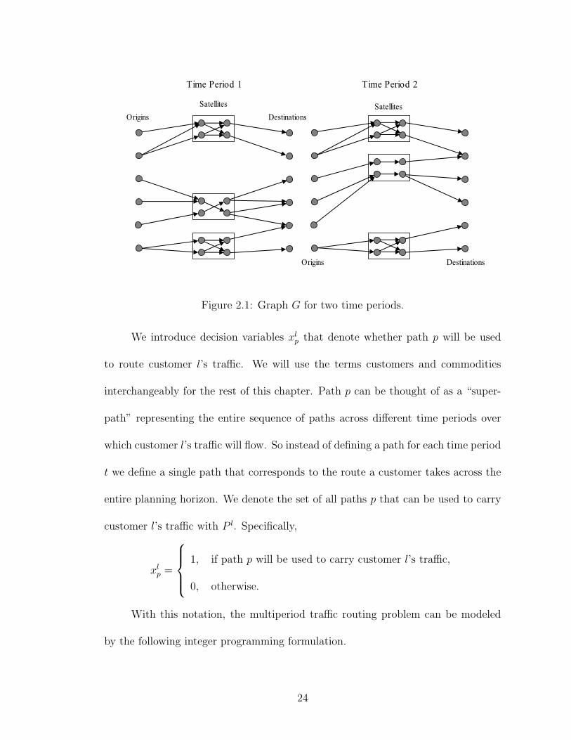
bij. Figure 2.1 provides an example of this graph for a two-period problem. Notice

that G is not connected and it is comprised of distinct components that represent

the state of the network at a specific time period t. We will refer to the component

(all nodes and arcs) that is associated with time period t, as Gt.

We denote the set of service requests that we wish to route with L. Each

service request, l, has an origin, destination and a demand dl that is a function of

time and can be positive only for consecutive time periods. Further, all demand for

each request must be routed on a single path (i.e., no demand splitting is allowed)

because all services require the use of continuous bandwidth segments. Our prob-

lem resembles a series of IMCF problems on each of the Gt components. While we

discuss the MPTR problem in the context of the satellite communications applica-

tion where it arose, we should note that our model and solution technique is quite

general and applies to MPTR problems on general graphs with (any type of) route

change penalties.

A flow based formulation for this graph would require an extremely large

number of flow variables f ltij (i.e., one for each arc (i, j), for each customer l and

time period t). Moreover, tracking the rerouting penalties with the use of flows would

require additional decision variables and constraints that would be able to capture

the differences |f l(t−1)ij − f lt

ij | for each arc (i, j) and each time period t = 2, . . . , T .

These extra variables and constraints make the flow-based approach intractable

even for a small number of time periods. Instead, we use a path-based formulation

quite similar to those discussed previously in the literature [5, 11, 45] for the IMCF

problem.

23

Time Period 1 Time Period 2

Satellites

Origins Destinations

Origins Destinations

Satellites

Figure 2.1: Graph G for two time periods.

We introduce decision variables xlp that denote whether path p will be used

to route customer l’s traffic. We will use the terms customers and commodities

interchangeably for the rest of this chapter. Path p can be thought of as a “super-

path” representing the entire sequence of paths across different time periods over

which customer l’s traffic will flow. So instead of defining a path for each time period

t we define a single path that corresponds to the route a customer takes across the

entire planning horizon. We denote the set of all paths p that can be used to carry

customer l’s traffic with P l. Specifically,

xlp =

1,

0,

if path p will be used to carry customer l’s traffic,

otherwise.

With this notation, the multiperiod traffic routing problem can be modeled

by the following integer programming formulation.

24

(MPTR) min∑

l∈L

∑

p∈P l

clpx

lp

subject to∑

l∈L

dlt

∑

p∈P l

δpijx

lp

≤ bij, ∀t, (i, j) ∈ At, (2.1)

∑

p∈P l

xlp = 1, ∀l ∈ L, (2.2)

xlp ∈ {0, 1}, ∀l ∈ L, p ∈ P l. (2.3)

In this model dlt represents the traffic demand for customer l in time period

t. δpij is one if path p uses arc (i, j) and zero otherwise. cl

p denotes the cost of path

p for customer l and includes the arc costs as well as the rerouting penalties for

super-path p. Specifically,

clp =

∑t

∑

(i,j)∈At

δpijd

ltcij +

∑t

eltγ

pt , (2.4)

where γpt is one if there is a rerouting for path p from period t − 1 to period t

(zero otherwise) and elt is the rerouting penalty cost for customer l in period t. We

defined the rerouting penalty so that it depends on the customer l because based

on theirs SLAs different customers will receive different discounts by the satellite

service provider. Also, notice that after the last time period in which a customer

has non-zero traffic demand we cannot have a rerouting. In the first time period in

the planning horizon t = 1, we might want to define rerouting penalties for all paths

other than the ones currently used by existing customers. In this way we can take

into consideration the current state of the network and not assume a “greenfield”

scenario.

25

In this model, the objective is to minimize the overall cost of routing the

demand while taking into account the rerouting penalties. Constraint set (2.1)

ensures that the capacity of an arc is not exceeded. Constraint set (2.2) ensures that

exactly one of all the possible super paths for each customer is selected. Notice that

even though we have defined the MPTR problem as a cost minimization problem

we can introduce profit information in the objective function coefficients clp and

maximize profits instead, depending on the application requirements.

2.4 Solution Approach

We now describe our solution approach for the multiperiod traffic routing

problem that uses the MPTR formulation in conjunction with a branch-and-price-

and-cut procedure.

2.4.1 Overview

To simplify the presentation and exposition in the rest of the dissertation, we

provide a brief overview of the BPC framework we use. In the BPC framework the

MPTR formulation describes what is known as the master problem (MP). Similar

to the standard branch-and-bound procedure, at each node in the BPC tree the

linear programming (LP) relaxation of the MP has to be solved (see Figure 2.2

for the steps inside a BPC node). Even though the MPTR contains a small num-

ber of constraints it has an exponential number of variables which means that the

solution of the corresponding LP requires the use of column generation. Column

26

generation solves the LP relaxation of the MP by only considering a small subset

of all the variables in the formulation. The MP that contains only a subset of

the variables is usually referred to as the restricted master problem (RMP). In the

column-generation procedure after solving the LP relaxation of a RMP one needs to

determine whether new columns (variables) have to be generated or whether the LP

relaxation of the corresponding MP has been solved to optimality. This is done by

solving the so-called pricing problem. The solution to the pricing problem provides

us with the new columns (here a column is an xlp variable or a super path p for

customer l) to add or verifies the optimality of the solution. After obtaining an

optimal solution for the LP the cutting phase adds violated valid inequalities to the

RMP. This cutting phase is in nature identical to the one found in branch-and-cut

procedures. Specifically, a separation problem is first solved to determine if any valid

inequalities are violated by the current linear solution. Once we add any inequali-

ties found during the cutting phase we solve the LP again. Notice that this requires

continuing the column-generation procedure and thus solving the pricing problem

again.

Our problem differs significantly from those studied previously in the litera-

ture [5, 11, 45] due to the rerouting penalties involved. Consequently, while the

structure of the MPTR path-based formulation is virtually identical to the path

based formulation for the IMCF problem, the BPC algorithms developed for the

IMCF cannot be applied to the MPTR problem. The reason being the solution to

the pricing problem for the IMCF problem no longer applies when there are route

change penalties. Instead, we now present a novel algorithm for solving the pricing

27

Begin

Step 0: Solve linear relaxation

Step 1: for all l ∈ L do

Solve pricing problem

end for

if there are any columns with negative reduced costs,

add them to the model and go to Step 0.

Step 2: for all {i, j} ∈ A do

Solve separation problem

end for

if there are any feasible inequalities,

add them to the master problem and go to Step 0.

End

Figure 2.2: Branch-and-price-and-cut algorithm.

28

problem of the MPTR formulation and some additional issues related to our BPC

approach.

2.4.2 Pricing

In the typical IMCF setting the pricing problem can be solved with the use

of a shortest-path algorithm on the original graph with slightly modified costs.

Specifically, the cost structure is usually defined in a way that allows the path costs

c′lp for commodity l, and super-path p, to be represented as the sum of the costs on

the path,∑

(i,j)∈A δpijcij. Notice that we use c′lp to denote the costs in the standard

IMCF problem in which we have routing costs only, as opposed to routing and

rerouting penalty costs. This in turn leads to the computation of the reduced cost

for path p and commodity l as,

c′l

p =∑

(i,j)∈A

dl(cij + πij)δpij − σl,

where −πij is the dual of the capacity constraints (2.1) and σl is the dual of the path

selection constraints (2.2). As a result, the cost of an arc (i, j) can be updated as

cij + πij and a shortest path algorithm can be used to find a path p for commodity

l with the smallest possible cost. If that cost times the demand, dl, is less than σl,

then the reduced cost of this path is negative and the path is added to the RMP

and the updated LP is re-optimized.

In the satellite routing problem the path variables xlp in MPTR represent a

series of paths that commodity l will follow across the different time periods in

the planning horizon. Therefore the cost of each super-path consists of an arc-cost

29

component and a rerouting component, as seen in equation (2.4). Specifically, the

reduced cost for path p and commodity l is given by,

clp =

∑t

∑

(i,j)∈At

dlt (cij + πij) δp

ij +∑

t

eltγ

pt − σl. (2.5)

Unfortunately, the reduced cost defined in (2.5) cannot be calculated by us-

ing the traditional approach that finds a shortest path on the original graph with

updated costs for a couple of reasons. First, the graph that models the problem is

not connected and therefore we cannot construct a single shortest path across all

time periods. More importantly, any approach that uses only the updated costs

of the arcs will fail to capture the rerouting penalties associated with some of the

super-paths. Therefore, in order to find the super-path p with the lowest reduced

cost for each commodity l we develop a technique that calculates the minimum cost

routing across all time periods while taking into account rerouting penalties.

The first step in this approach involves solving a K-shortest path problem

on Gt, between the customer’s origin and destination, for each time period t in

which that customer has positive demand. The arc costs, on graph Gt are updated

with the dual values of the capacity constraints πij in exactly the same way as in

the traditional pricing problem approach (i.e., cij + πij). The number of paths Kt

that we need to find in time period t is not fixed and can be different for different

commodities and time periods. We will specifically discuss how Kt is determined

later in this section. Once we have found the Kt shortest paths for each time period

we then construct a “multiperiod routing graph” G′ = (N ′, A′) in which the node

30

set consists of a dummy origin node, a dummy destination node, and one node for

each of the shortest paths found in each time period. We augment this graph with

arcs from the origin node to all first period nodes (i.e., nodes that represent paths in

the first period that a customer has positive demand) and arcs from the last period

nodes (i.e., nodes that represent paths in the last period that a customer has positive

demand) to the destination node. Furthermore we connect all nodes from period

t−1 to the nodes in period t and set the cost, hij, of an arc (i, j) equal to h(qj)+elt,

where h(qj) is the cost of the path, qj represented by node j taking into account the

demand. elt is the penalty cost introduced only if the path qj represented by node

j is different from the path qi represented by node i. Note that in a more general

setting the rerouting penalty can be a function of the specific paths used in periods

t − 1 and t. We explore this possibility in Section 3.4.1. In the satellite planning

context two paths in two different time periods are considered to be different when

any of the arcs they include represent different communication links (i.e., origin

to up-beam, onboard, or down-beam to destination links) or they represent the

same links onboard the same satellite but the satellite has been relocated to a new

longitude. For arcs (i, j) where i is the dummy origin node we introduce no penalty

cost1 (i.e., hij = h(qj)) and when j is the dummy destination node we set hij = 0.

Notice that a path in the multiperiod routing graph represents a super-path p in

MPTR. Specifically, the nodes that are used in the path on G′ (apart from the

dummy origin and destination nodes) represent paths in G and therefore there is

1In practice, we might want to introduce penalties even when i is the dummy origin node so

that we can account for rerouting of existing service requests.

31

Dummy

Origin

Dummy

Destination

Period 1

Paths

Period 2

Paths

Zero cost Cost of path at the

head of the arc

+

potential rerouting

cost

Cost of path at the

head of the arc

Figure 2.3: Multiperiod routing graph, G′, for a problem with 2 time periods and 3

paths per period.

a one-to-one correspondence between the paths in G′ and the super-paths in G.

Figure 2.3 presents the multiperiod routing graph for a problem with 2 time periods

in which 3 shortest paths have been calculated for each period.

Once the construction of the multiperiod routing graph is complete we solve

a shortest path problem from the dummy origin node to the dummy destination

node. The cost of this path is then compared to the dual variable σl and if it is

smaller we add the corresponding super-path p to our model. If the cost of the path

is larger than the dual variable of the path selection constraints, then there are no

super-paths for commodity l that can improve the current solution. Naturally, we

have to repeat the same process for all commodities l in our model. Notice that the

32

original graph G (and all of its components) needs to be updated only once since

the updates are common for all commodities.

In order to ensure that this procedure obtains the super-path with the lowest

(reduced) cost we need to define the number of paths Kt that have to be included

in time period t. Instead of generating all paths for a time period, we specify the

following sufficient condition that can be used to determine whether a specific choice

of {K1, K2, . . . , KT} ensures that we have found the lowest cost super-path. Let qtn

denote the nth shortest path in time period t. Let Rt = {qt1, q

t2, . . . , q

tKt} denote the

set of Kt-shortest paths in time period t and P t denote the set of all feasible paths

in time period t.

Proposition 2.1 The multiperiod routing graph G′ contains a lowest cost super-

path p, if h(qtKt

)− h(qt1) ≥ 2el

t or Rt = P t, for t = {1, . . . , T}.

Proof: Suppose not. Then for some time period t, Rt 6= P t because otherwise the

pricing graph G′ will contain all feasible paths and therefore the lowest cost super-

path. Let p∗ be a lowest cost super-path. Then for some time period t (in which

Rt 6= P t), p∗ contains a path qtj distinct from qt

1, . . . , qtKt

, (i.e., j > Kt) and therefore

h(qtj) ≥ h(qt

Kt). By replacing path qt

j by path qt1 in super-path p∗ we can get a

super-path with cost less than or equal to p∗, since h(qtKt

)− h(qt1) ≥ 2el

t and in the

worst case we will incur one penalty going from t − 1 to t and another one going

from t to t + 1. Consequently this new super-path is also optimal. Repeating this

procedure for each time period t in which p∗ contains paths distinct from qt1, . . . , q

tKt

,

we obtain a lowest cost super path that belongs to G′.

33

It is actually possible to generate significantly fewer paths in each time period.

This is critical, since the time spent in pricing will be a function of the number of

paths we generate. To explain how, we need some additional notation. For each

time period t, we define four quantities ta, tb, tc, and td. Let

ta =

T − t, if h(qiKi

)− h(qi1) ≤ 2el

i and Ri 6= P i, for i = t, t + 1, . . . , T ,

min{i ∈ [0, T − t] : h(qt+iKt+i

)− h(qt+i1 ) > 2el

t+i or Rt+i = P t+i}, otherwise.

Here ta tells us the first occurrence, in terms of the number of time periods after t, of

a time period where either the cost of the Kth-shortest path (actually Kt+ta-shortest

path in time period t+ ta) is greater than the cost of the shortest path for that time

period plus two times the rerouting penalty, or the time period has generated all

possible paths between the origin and destination. If no such time period exists

then ta is defined as T − t, the largest possible value it could take. Similarly, let

tb =

t− 1, if h(qiKi

)− h(qi1) ≤ 2el

i and Ri 6= P i, for i = 1, 2, . . . , t,

min{i ∈ [0, t− 1] : h(qt−iKt−i

)− h(qt−i1 ) > 2el

t−i or Rt−i = P t−i}, otherwise.

Here tb is similar to ta except that we are now looking for the first time period prior

to (and including) time period t. Let

tc =

T − t, if h(qiKi

)− h(qi1) ≤ 2el

i and Ri 6= P i, for i = t, t + 1, . . . , T ,

0, if ta = 0,

ta − 1, otherwise.

Here tc tells us the number of consecutive time periods after t for which h(qiKi

) −

34

h(qi1) ≤ 2el

i and Ri 6= P i. Similarly, let

td =

t− 1, if h(qiKi

)− h(qi1) ≤ 2el

i and Ri 6= P i, for i = 1, 2, . . . , t,

0, if tb = 0,

tb − 1, otherwise.

Here td is similar to tc except that we are looking for the number of consecutive time

periods prior to t for which h(qiKi

)− h(qi1) ≤ 2el

i and Ri 6= P i.

For a given path qrj in time period r, we are interested in knowing whether this

path is feasible in another time period t. Let F t(qrj ) = ∅ if path qr

j does not exist in

time period t, and F t(qrj ) = qt

k for some positive k if the path exists in time period t

(i.e., F t(qrj ) ∈ P t). In other words F t(.) is a mapping of a path to time period t, that

tells us whether that path is feasible in time period t. When F t(.) is applied to a set

of paths A = {a1, a2, . . . , an}, it outputs the set of paths obtained by applying F t(.)

to each of the paths in A. That is, F t(A) = {F t(a1), Ft(a2), . . . , F

t(an)}. Let Rst be

the set of paths from Rs that are valid for time period t. That is, Rst = F t(Rs).

We now describe two methods to generate significantly fewer paths in each

time period. Let Qt =⋃r=t+ta

r=t−tbRr

t\Rt. Qt includes all the Kr shortest paths from

time periods r = t− tb to r = t+ ta that are distinct from Rt (the Kt shortest paths

in time period t) and valid for time period t. Notice, when h(qtKt

)− h(qt1) > 2el

t or

Rt = P t, Qt = ∅. Also, observe that the cost of any path in Qt is greater than or

equal to the cost of all of the paths in Rt. Let St = Rt ∪Qt.

We construct the “multiperiod routing graph” G′ as described before, except

that the set of nodes (i.e., paths) in time period t are created from the set St (i.e.,

we create one node in time period t for each of the paths in St). We now show that

35

if we ensurer=t+tc⋂r=t−td

F t(Rr) 6= ∅ t = 1, . . . , T, (2.6)

then the multiperiod routing graph G′ is guaranteed to contain a lowest cost super-

path. Condition (2.6) says that when there is at least one common path for every

maximal set of consecutive time periods that satisfy h(qiKi

)− h(qi1) ≤ 2el

i and Ri 6=

P i, the multiperiod routing graph G′ contains a lowest cost super-path.

Theorem 2.1 When Condition (2.6) is satisfied, the multiperiod routing graph G′

contains a lowest cost super-path.

Proof: Suppose not. Let p∗ be a lowest cost super-path. Then there is some time

period r in which p∗ contains a path qrj that does not belong to Sr. If ra = rb = 0,

then either Rr = P r or h(qrKr

)− h(qr1) > 2el

r. In the former case qrj ∈ Rr = Sr and

we have a contradiction. In the latter case, replacing path qrj by path qr

1 strictly

reduces the cost of the super-path yielding a contradiction.

Consequently, assume ra + rb > 0. Further, consider the subcase where ra =

rc + 1 and rb = rd + 1. The proofs of the other three subcases: (1) ra = rc = T − t

and rb = rd = t − 1, (2) ra = rc + 1 and rb = rd, and (3) ra = rc and rb = rd + 1,

follow analogously. Let

jrα = max{i : 0 ≤ i ≤ ra and qr

j , Fr+1(qr

j ), . . . , Fr+i(qr

j ) ∈ p∗},

Loosely speaking, starting at time period r, jrα denotes the number of time periods

after time period r that the path F t(qrj ) appears consecutively in the super-path p∗.

Similarly, let

jrβ = max{i : 0 ≤ i ≤ rb and F r−i(qr

j ), . . . , Fr−1(qr

j ), qrj ∈ p∗}.

36

In other words, the super-path p∗ consists of path qrj repeatedly between time

periods r − jrβ and r + jr

α with no route change penalty. Specifically, F r−jrβ(qr

j ),

F r−jrβ+1(qr

j ),. . ., F r−1(qrj ), qr

j , F r+1(qrj ),. . ., F r+jr

α(qrj ) ∈ p∗.

Note that F t(qrj ) 6∈ St for t = r − rb, . . . , r + ra. Otherwise, the path F t(qr

j )

would be in Rt for some t = r − rb, . . . , r + ra, and as a result it would also be in

St for all t = r − rb, . . . , r + ra. If jrα = ra, then in time period r + ra, F r+ra(qr

j )

belongs to p∗. But, since replacing F r+ra(qrj ) by qr+ra

1 strictly decreases the cost of

the super-path (because for t = r + ra, h(F t(qrj )) ≥ h(qt

Kt) > h(qt

1) + 2elt, this is

not possible (the other possibility Rr+ra = P r+ra is eliminated since F t(qrj ) 6∈ St

for t = r + ra). Thus jrα < ra (and jr

α ≤ rc). Arguing similarly, jrβ < rb (and

jrβ ≤ rd). Let qr

k be a common path across Rr−rd , . . . , Rr, . . . , Rr+rc . Specifically,

qrk ∈

⋂t=r+rc

t=r−rdF r(Rt). Observe that h(F t(qr

k)) ≤ h(F t(qrj )) for t = r − jr

β, . . . , r + jrα.

By replacing path F t(qrj ) by path F t(qr

k) in time periods t = r−jrβ, . . . , r+jr

α we get

a super-path with cost less than or equal to p∗. Consequently, this new super-path

is also optimal. Repeating this argument for time periods where p∗ contains a path

qrj that does not belong to Sr completes the proof.

In our second method to reduce the number of paths in G′ we define, Qt =

⋃r=Tr=1 Rr

t\Rt. Qt now includes all the Kr shortest paths from time periods r = 1 to

r = T that are distinct from Rt and valid for time period t. Observe that the cost

of any path in Qt is greater than or equal to the cost of all of the paths in Rt. Like

the first method, the “multiperiod routing graph” G′ is constructed as before, with

the set of nodes in time period t created from the set St = Rt ∪ Qt. We now show

37

that if we ensure

h(qtKt

)− h(qt1) ≥ el

t or Rt = P t t = 1, . . . , T, (2.7)

then the multiperiod graph G′ is guaranteed to contain the lowest cost super-path.

Theorem 2.2 When Condition (2.7) is satisfied, the multiperiod routing graph G′

contains the lowest cost super-path.

Proof: Suppose not. Let p∗ be a lowest cost super-path. Then for some time period

r, p∗ contains a path qrj not in Sr. Let

jrα = max{i : 0 ≤ i ≤ T − t and qr

j , Fr+1(qr

j ), . . . , Fr+i(qr

j ) ∈ p∗},

and

jrβ = max{i : 0 ≤ i ≤ t− 1 and F r−i(qr

j ), . . . , Fr−1(qr

j ), qrj ∈ p∗}.

Observe, that the paths F r+i(qrj ) for i = 0, . . . , jr

α and the paths F r−i(qrj ) for

i = 0, . . . , jrβ do not belong in Si for i = r−jr

β, . . . , r, . . . , r+jrα. We construct a new

super-path by replacing the path F i(qrj ) by qi

1 in time periods i = r−jrα, . . . , r, . . . , jr

β.

Notice that by using the new paths we incur jrα + jr

β extra penalties. However,

h(F i(qrj )) ≥ h(qi

K) ≥ h(qi1)+el

i, for all i = r−jrβ, . . . , r+jr

α and∑r+jr

αi=r−jr

βh(F i(qr

j )) ≥∑r+jr

αi=r−jr

β(h(qi

1) + eli) >

∑r+jrα

i=r−jrβh(qi

1) + (jrα + jr

β)eli. As a result the new super-path

has a cost that is strictly lower than the cost of p∗ which contradicts our initial claim

that p∗ is the lowest cost super-path.

In our implementation we generate a small number of paths, say κt, for each

commodity and each period t and then check to see whether Condition (2.6) or

38

Condition (2.7) is satisfied. If neither of these two conditions are satisfied, we then

generate the next set of κt shortest paths for all time periods in which Rt 6= P t

(i.e., we haven’t generated all feasible paths). This is repeated, until either Con-

dition (2.6) or Condition (2.7) is satisfied and the appropriate multiperiod routing

graph is constructed. Notice that by saving the state of the K-shortest path al-

gorithm in each time period it is possible to determine the next set of κt shortest

paths without having to recompute paths that were already found.

2.4.3 Cutting

Barnhart et al. [11] observe that IMCF problems exhibit symmetry effects

that make them hard to solve when using solely a branch-and-price approach. Sym-

metry refers to the fact that the objective value of the problem hardly changes after

branching. In order to understand why the objective remains unchanged consider

the following example. Let d1, d2 and d3 be the demands for commodities 1, 2 and

3, respectively. Also, assume that these commodities have the same origin and des-

tination and in the current linear solution 1 and 2 are both using arc (i, j) while 3 is

using some other arc. Additionally let x1p (that carries the demand for commodity

1) be integer and x2p (which refers to the path for commodity 2) be fractional. If we

branch on x2p and force it off of arc (i, j) then it will simply be replaced by x3

p. If

on the other hand we force it on arc (i, j) then x1p will become fractional. Because

of this symmetry, it is necessary to generate cutting planes that define facets of the

problem polytope that help eliminate the symmetry. Essentially, these inequalities

39

say that sets of commodities (similar to the ones in our example) cannot use a

specific arc at the same time.

For the standard IMCF problem the capacity constraints (which are identi-

cal to (2.1)) when translated to a node-arc (or flow-based) representation define 0-1

knapsack inequalities. Even though the entire representation of the MPTR formula-

tion in node-arc form (i.e., with flow variables) would not be viable, as noted earlier

(Section 2.3), we can still look at the node-arc form of the capacity constraints

for the purposes of this exposition only. We introduce the arc flow variables f lij,

which are one if commodity l is using arc (i, j) and zero otherwise. The capacity

constraints can then be written as,

∑

l∈L

dltf

lij ≤ bij, ∀t, (i, j) ∈ At.

We can now use lifted cover inequalities (LCI) to strengthen the formulation

and reduce the symmetry effects. The general form of a LCI with respect to the arc

flow variables is,

∑

l∈C

f lij +

∑

l∈C

αlflij ≤ |C| − 1,

where the set C defines a minimal cover2, C = L\C and αl is the lifting coefficient

for commodity l. By using the flow decomposition theorem (see [4]), that states

f lij =

∑

p∈P l

δpijx

lp,

2A set C ⊆ L is a cover if∑

l∈C dlt > bij . A cover is minimal if C \ {l} is not a cover for any

l ∈ C.

40

we can go from the LCI written in terms of flow variables to the LCI written in

terms of the path variables as,

∑

l∈C

∑

p∈P l

δpijx

lp +

∑

l∈C

αl

∑

p∈P l

δpijx

lp ≤ |C| − 1.

In practice after we solve the LP of the MP to optimality using column-

generation and the pricing procedure presented earlier we look at all the arcs of

G that are saturated (i.e., have zero slack). We then create a cover C (similar to

[38]) by inserting into C first the commodities for which f lij = 1 and then f l

ij < 1 so

that∑

l∈C dlt > bij. We then delete any commodities from the cover so as to make it

minimal and then use the sequence independent lifting procedure proposed by Gu

et al. [39] to find the lifting coefficients αl. Using this approach we generated one

LCI for each saturated arc and added all such LCIs into our model. The LP of the

RMP is then re-solved and the pricing procedure generates any necessary additional

columns. Notice that the cost of the arcs in G will now have to be updated with the

dual variables of the LCI constraints as well. Specifically, when solving the pricing

problem for commodity l the cost of arc (i, j) is updated as,3

cij + πij +∑m∈M

αml

ζm

dlt

where M is the set of all LCIs that refer to arc (i, j) ∈ A, αml is the lifting coefficient

of commodity l in the mth inequality and −ζm is the dual of that inequality, where

ζm is non-negative. Note that the new costs depend on which commodity l we

3In Barnhart et al. [11] the new cost of arcs (i, j) are mistakenly updated by αml ζm instead of

αml ζm/dl

t.

41

are solving the pricing problem for, and as a result have to be updated for each

commodity.

In our BPC approach we generate cuts with the procedure described above

whenever possible and add them to the current model. Since these cuts are globally

valid we also add all of these cuts to a global cut pool. At the start of each node

in the BPC tree the cut pool is compared against the cuts currently in the node

and any cuts that are missing from the node are added before solving the LP of the

RMP.

2.4.4 Other Considerations

In this section we discuss some additional issues related to the BPC procedure.

Branching

In branch-and-price procedures branching presents an additional challenge

since branching rules should not be allowed to interfere with the structure of the

pricing problem. Barnhart et al. [11] have developed a very successful branching

rule for IMCF problems, which we applied in our procedure. The branching rule

finds the first node for which two fractional paths of the same commodity, l, di-

verge and partitions the set of arcs emanating from that node. The partition is

constructed so that the arcs used by the fractional paths of the commodity belong

to two different sets, I and I. In the first branch commodity l is not allowed to use

the arcs in I, while in the second branch commodity l is not allowed to use the arcs

42

in I. In our case this branching rule can be easily enforced by deleting the arcs from

the appropriate set when solving the pricing problem for commodity l. By deleting

these arcs we ensure that when finding the K-shortest paths for commodity l we

will consider no paths and – as a result – no super-paths that use these arcs.

Feasibility

Another issue that arises with the use of column-generation procedures is

the initial feasibility of the LP relaxation of the RMP (since it doesn’t include all

possible variables). The standard practice that is used to ensure feasibility of the LP

at all nodes in the B&B tree is the inclusion of auxiliary columns with appropriate

coefficients for the constraints and costs in the objective function (see [12, 30, 82]).

In the case of the MPTR problem we add one super-path for each commodity. These

“feasibility” paths will have a coefficient equal to one for the constraints which ensure

that exactly one path is chosen (2.2) and a cost that must be greater than the cost

of all the other paths for that commodity. The cost coefficient for these paths is

largely irrelevant and only ensures that these paths will not be favored over regular

paths in the model.

With the addition of the “feasibility” paths we have ensured that we are going

to find a feasible solution when all demand can be met. However, in the case of the

MPTR problem and practical applications of the IMCF problem we would still like

to get an IP solution when some of the requests cannot be routed because of traffic

congestion in the network. For this reason we need to add special arcs that carry

43

flow directly (i.e., bypassing the network) from the origin to the destination. We

refer to these as “unmet demand” arcs and we add them to our graph G. Specifically,

we augment graph G with two unmet demand nodes and one unmet demand arc

for each time period. All origin nodes in a time period are then connected to the

node at the tail of the unmet demand arc. Also, the node at the head of the unmet

demand arc is connected to all destination nodes at this time period. The unmet

demand arcs have a cost per unit of flow equal to the opportunity cost of not offering

service to a customer (i.e., the revenue for a customer) and have unlimited capacity.

In Figure 2.4 we provide an example of these unmet demand arcs. All of these

arcs are represented in our pricing graph G′ with “unmet demand” nodes, where we

have one node for each arc. There are two ways in which we can use these nodes

depending on how we wish to model unmet demand in our problem. The first option

is to connect the unmet node in period t− 1 only with the unmet node in period t,

for all time periods. Naturally, the unmet node in the first period is connected to

the dummy origin node in G′ and the unmet node in the last period is connected

to the dummy destination node. This way we allow for one super-path in the RMP

(for each commodity) that will represent unmet demand across all time periods and

will result in our model either routing customers or denying them service for the

entire planning horizon. The second option is to introduce arcs that will connect all

the nodes in period t− 1 with the unmet node in period t, and the unmet node in t

with all the nodes in t + 1, for all time periods. Under this scenario we will be able

to consider super-paths that allow a commodity to be routed for some periods, then

dropped and then possibly routed again. The first option is probably better suited

44

for actual planning purposes since a satellite provider is usually unwilling to stop

servicing an existing customer because of the associated, high ill-will costs. However,

the second option provides us with the possibility of considering these ill-will costs

in the model (if we desire to do so) and is more appropriate when comparing the

results of the MPTR formulation with a period-by-period optimization approach (as

we do in Section 2.5). In our implementation we assign a cost to the arc that leads

to the unmet node in period t equal to the revenue generated by the service request

at period t (plus the appropriate penalty and ill-will costs). With this technique

even in cases when all demand cannot be routed we still get a feasible solution that

minimizes costs.

In both cases it is necessary for branching to take into account (and eliminate)

fractional unmet demand. We achieve this by enforcing the branching rules by

deleting appropriate arcs on the graph, G. Specifically, during the branching process

we look for fractional flow through the unmet demand arcs. If there is such flow

we need to determine the time period at which the two fractional paths (the one

that carries unmet demand and the one that carries demand that is met) diverge

and create one branch in which we exclude the unmet arc from consideration and

another branch in which we exclude the arc that carries demand that is met. By

deleting these arcs the associated pricing graph that is going to be built will lack

either the unmet demand node or the path that corresponds to the arc that carries

demand that is met. Notice that we delete these arcs only when solving the pricing

problem for the customer associated with the branching restriction. The pricing

problem for all other customers should consider these arcs as usual. In Figure 2.4

45

Origins Destinations

Satellites

Unmet Arc

Origins Destinations

Satellites

Unmet Arc

Origins Destinations

Satellites

Unmet Arc

Root Node

Branch 1 Branch 2

Fractional Commodity

Figure 2.4: Example of a node with a fractional customer over an unmet demand

arc and the associated branching implementation. Notice that in “Branch 1” we

have deleted an arc representing an onboard connection and in “Branch 2” we have

deleted the unmet arc.

we provide an example of a customer with fractional flow and show the changes in

the network for the two branches.

2.5 Computational Results

We now present several computational experiments on various data sets. Most

of the characteristics of our problem sets are designed to replicate the key attributes

of real-life satellite networks and are pertinent to the multiperiod traffic routing

problem. We were able to obtain the attributes of actual satellite networks after

46

repeated interactions with leading companies in the satellite industry. Our com-

putational work is split into two main directions. First we look at the benefits of

applying a multiperiod optimization procedure as opposed to a period-by-period

optimization process for varying problem characteristics. Then we compare the full

blown BPC procedure with a “Root-Node” procedure that uses column-generation

only at the root node of the B&B tree and only generates cuts (as opposed to cuts

and columns) during the entire search. The BPC and Root-Node procedures were

coded in C++ with the use of ILOG CPLEX v9.0 and the ILOG Maestro libraries,

while the period-by-period process uses only ILOG CPLEX v9.0. All computational

work was conducted on a Pentium IV Xeon processor, with 3 GHz clock speed and

2 GB of RAM.

Our computational analysis is done on randomly generated problem sets (see

Table 2.1). Each problem set contains 20 instances. The problems correspond

to a network with 2 satellites (approximately 100 nodes and 280 arcs in each time

period) and a planning horizon of 5 time periods. The arcs representing the onboard

connections of the satellites have an average capacity of 2 traffic units4 and an

average cost of $200, 000 (per traffic unit per time period). The network consists of

10 regions that can act as origins and destinations for each of the 50 customers that

have average demands of 0.8 traffic units. The demand for each customer is drawn

in each period from a uniform distribution on the interval [0.75, 0.85]. A customer

that is generated in period t has a 90% chance of “surviving” in the next period

and in each period after the first we generate 5 new customers. The unmet demand

4One traffic unit is typically equivalent to 36MHz of bandwidth.

47

Parameter Description Value

Network

# of regions 10

# of time periods 5

# of satellites per period 2

# of onboard connections per satellite 8

Capacity of onboard connections ∼ U [1, 3]

Cost per unit of capacity ∼ U [$150, 000, $300, 000]

Demand

# of customers per time period 50

Demand of each customer ∼ U [0.75, 0.85]

Survival probability for a customer 0.9

New customers in each period 5

Unmet demand cost $750, 000

Rerouting penalty cost $300, 000

Table 2.1: Problem parameters used in the random problem generation.

48

cost was set to $750, 000 (per traffic unit per time period), which approximates

the average revenue generated by a satellite customer (leasing 1 traffic unit) over

a one year period. The rerouting penalties in the satellite industry are usually

defined as discounts that are offered to the affected customers and are typically set

to 40%. The rerouting penalty was therefore set to $300, 000 (per traffic unit per

time period). In order to replicate the dynamic topology of satellite networks we

also define a survival probability for the onboard connections (instead of modeling

launches, relocations and discontinuation of service for entire satellites) which we

set to 90%, so roughly 10% of the onboard links will be re-configured in each period.

The set of attributes that we have defined comprise a baseline problem scenario.

Individual characteristics of this baseline are then altered so as to explore different

aspects of the multiperiod traffic routing problem.

2.5.1 Multiperiod vs. Period-by-Period

From a practical standpoint it is important to provide tangible proof to all

professionals in the industry as to the benefits of a multiperiod approach over a

period-by-period optimization process. By period-by-period optimization we refer

to the process of myopically routing all of the commodities in period t and then

looking at the routing problem for the next period, t + 1, without being able to

change any of the routes in period t. We achieve this solution with the use of a

typical flow-based formulation. The formulation uses the variables f ltij , which are

one if commodity l is using arc (i, j), in time period t and zero otherwise. We now

49

present the period specific routing (PSR) formulation for period t,

(PSRt) min∑

l∈L

∑

(i,j)∈At

cltijf

ltij (2.8)

subject to∑

j:(j,i)∈At

f ltji −

∑

j:(i,j)∈At

f ltij = olt

i ∀i ∈ Vt, l ∈ L, (2.9)

∑

l∈L

dltf

ltij ≤ bij, ∀t, (i, j) ∈ At, (2.10)

f ltij ∈ {0, 1}, ∀l ∈ L, (i, j) ∈ At. (2.11)

where olti is equal to −1 or 1 if i is the origin node or destination node of commodity

l at time period t, respectively and zero otherwise. Note that we avoid infeasibility

when all demand cannot be met by augmenting the set At with arcs going from

the origin node to the destination node of each commodity and for all time periods.

These arcs have cost equal to the unmet demand cost, for each commodity l and

time period t. In order to take into account the rerouting penalties we have two

options. Solve the PSR problem for each time period without penalties and then

add the penalties based on the solution. Observe that this approach might be the

only option in the MPTR problem on general graphs. However, in the case of

the satellite network the rerouting penalties are effectively applied only when the

onboard connection used changes. Thus we can incorporate the cost of a route

change penalty by modifying the cost cij of the arcs corresponding to the onboard

connections. Therefore we set cltij equal to cijd

lt+el

t (where elt is the rerouting penalty)

if commodity l has not used arc (i, j) in period t−1 and (i, j) represents an onboard

connection. We make this change in order to allow the period-by-period approach

to take into account, at some level, the route change penalties.

50

Table 2.2 presents computational results for the BPC and period-by-period

approaches on five different problem sets. These problem sets are characterized

by a varying load-factor, which we define as the ratio of the total demand over

the aggregate capacity in the network (in each period). The first column in the

table specifies the load-factor generated in each time period for each problem set.

The second and third columns present the solution found by the period-by-period

approach and the time (in seconds) required to reach that solution, respectively.

The three columns under the heading “Multiperiod (BPC)” specify the best primal

solution found by the BPC procedure, the percentage gap of that solution to the best

dual bound, and the running time (all running times are reported in seconds). Note

that the runs of the BPC procedure were limited to 1 hour. The last two columns

in the table give the average percentage gap between the solution of the period-

by-period approach and the BPC procedure. The first column reports the average

over all 20 instances in each set while the second column presents the average only

over the instances in which BPC converged (i.e., solved the problem to optimality

within the allotted 1 hour). The runs were conducted using the second of the two

options for dealing with unmet demand (see Section 2.4.4) and for both procedures

customers were not allowed to be routed in the future once they had been denied

service at some point in the past. In the period-by-period approach we achieve this

by setting the flow variable on the unmet demand arc equal to one for each time

period, t after the one in which the customer was routed over an unmet demand arc.

The same effect can be achieved in the multiperiod procedure when constructing

the multiperiod pricing graph G′ by allowing only one outgoing arc from the node

51

that represents the unmet path in period t to the node that represents the unmet

path in period t + 1. Also, for both procedures we imposed an extra penalty when

a customer that was routed is dropped in some future time period. This penalty

represents the ill-will cost associated with denying service to an existing customer

and we set it equal to the unmet demand cost. The results show that as the load

factor increases the instances become harder and the BPC procedure does not always

converge within the time limit set. Looking at the averages for instances that have

converged we see that savings between 7.4% and 11.3% can be achieved with the

use of a multiperiod as opposed to a period-by-period approach.

Table 2.3 provides another comparison between the multiperiod and period-by-

period approaches on four different problem sets. The table has the same structure

as before and the problem sets are characterized by different rerouting penalties.

This table can provide some insight as to when the rerouting penalty value is high

enough to make the use of a multiperiod approach beneficial. Observe that for

the extreme case in which the rerouting penalty is zero (e.g., on terrestrial fiber

optic traffic routing) the period-by-period approach can be, in theory, as good as a

multiperiod approach. However, other restrictions, such as the fact that we do not

allow for customers that have been dropped to be routed in future time periods and

the fact that we impose an extra penalty for dropping customers will always allow

a multiperiod approach to maintain the advantage. This is evident from the small

gap (i.e., 0.86%) reported for instances that have converged. In Table 2.3 the first

column gives us the penalty value as a percentage of the unmet demand cost used

(i.e., $750, 000). Note that for high values of the rerouting penalty the difference

52

between the two approaches becomes as high as 24.3%. For a rerouting penalty

equal to zero the period-by-period approach actually does better when looking at

the average over all the instances (i.e., −2.71%). Obviously, this is due to the fact

that we used a 1 hour time limit for all problem runs. From this comparison we can

have a clear indication as to the effect of the rerouting penalty size and gauge the

potential benefits of a multiperiod vs. a period-by-period approach as that penalty

changes.

Tables 2.4 and 2.5 compare the two approaches as the number of time periods

and the number of customers increases. Observe that the running time for the BPC

algorithm does not increase significantly as the number of periods increases. The

same is not true however for increasing number of customers. This is an indication

that our BPC procedure is not adversely affected by the size of the planning horizon

but larger number of commodities can require significantly more time to solve. We

believe that this can be attributed to the characteristics of our approach to the

pricing problem. Specifically, additional time periods only require us to add a few

extra nodes to the pricing graph and the solution of a shortest path problem on a

slightly larger graph. However, additional commodities require the construction of

extra pricing graphs at each node of the BPC tree. Also, observe that the percentage

gap between the solutions for the two procedures remains relatively constant in

Tables 2.2, 2.4 and 2.5. This is a another indication of the considerable effect of

the rerouting penalty on MPTR problems and the value of applying a multiperiod

approach when that penalty is significant.

53

Loa

dPer

iod-b

y-P

erio

dM

ult

iper

iod

(BP

C)

Pri

mal

Gap

s(%

)

Fac

tor

Pri

mal

($)

Tim

e(s

)P

rim

al($

)G

ap(%

)T

ime

(s)

Ove

rall

Con

verg

ed

0.4

33,4

47,0

400.

8130

,722

,473

0.00

7.67

8.89

8.89

0.5

44,2

38,9

500.

8240

,846

,284

0.00

38.5

48.

338.

33

0.6

59,7

52,8

050.

9055

,682

,480

0.00

302.

457.

357.

35

0.7

77,6

43,4

371.

0174

,412

,575

3.64

1,23

2.34

4.88

8.23

0.8

105,

666,

374

1.12

99,2

14,4

274.

511,

469.

237.

2711

.34

Tab

le2.

2:C

ompar

ison

ofPer

iod-b

y-P

erio

dto

Mult

iper

iod

opti

miz

atio

nfo

rdiff

eren

tlo

ad-fac

tors

.

Pen

alty

Per

iod-b

y-P

erio

dM

ult

iper

iod

(BP

C)

Pri

mal

Gap

s(%

)

(%of

unm

etco

st)

Pri

mal

($)

Tim

e(s

)P

rim

al($

)G

ap(%

)T

ime

(s)

Ove

rall

Con

verg

ed

100

54,1

54,9

600.

7643

,615

,768

0.00

47.2

824

.32

24.3

2

5044

,238

,950

0.82

40,8

46,2

840.

0038

.54

8.33

8.33

1039

,080

,372

0.80

38,4

12,1

580.

8062

0.58

1.78

2.51

036

,269

,020

0.94

37,1

53,7

803.

503,

469.

66-2

.71

0.86

Tab

le2.

3:C

ompar

ison

ofPer

iod-b

y-P

erio

dto

Mult

iper

iod

opti

miz

atio

nfo

rdiff

eren

tre

routi

ng

pen

alty

valu

es.

54

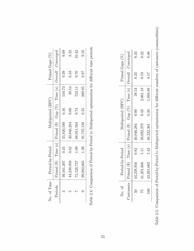
No.

ofT

ime

Per

iod-b

y-P

erio

dM

ult

iper

iod

(BP

C)

Pri

mal

Gap

s(%

)

Per

iods

Pri

mal

($)

Tim

e(s

)P

rim

al($

)G

ap(%

)T

ime

(s)

Ove

rall

Con

verg

ed

339

,161

,207

0.45

35,8

20,5

990.

1651

0.73

9.39

9.09

544

,238

,950

0.82

40,8

46,2

840.

0038

.54

8.33

8.33

775

,528

,737

1.09

68,9

11,5

040.

7475

2.11

9.70

10.4

2

999

,882

,605

1.39

91,7

35,1

380.

3588

0.85

8.87

9.10

Tab

le2.

4:C

ompar

ison

ofPer

iod-b

y-P

erio

dto

Mult

iper

iod

opti

miz

atio

nfo

rdiff

eren

tti

me

per

iods.

No.

ofPer

iod-b

y-P

erio

dM

ult

iper

iod

(BP

C)

Pri

mal

Gap

s(%

)

Cust

omer

sP

rim

al($

)T

ime

(s)

Pri

mal

($)

Gap

(%)

Tim

e(s

)O

vera

llC

onve

rged

5044

,238

,950

0.82

40,8

46,2

840.

0038

.54

8.33

8.33

7541

,201

,868

1.11

38,0

92,3

790.

432,

061.

198.

198.

32

100

43,2

61,0

021.

4340

,232

,361

0.49

1,89

4.89

8.17

8.08

Tab

le2.

5:C

ompar

ison

ofPer

iod-b

y-P

erio

dto

Mult

iper

iod

opti

miz

atio

nfo

rdiff

eren

tnum

ber

sof

cust

omer

s(c

omm

odit

ies)

.

55

2.5.2 BPC vs. Root-Node

It is common in the mathematical programming literature to compare branch-

and-price procedures with heuristic approaches that use column-generation only at

the root node and then go through the B&B tree without introducing new variables.

These comparisons are usually indicative of the potential benefits of generating

columns throughout the B&B tree but can also suggest that column-generation

at the root node only can be used as a heuristic in practice without a significant

disadvantage.

In Tables 2.6, 2.7 and 2.8 we present results that are generated by the BPC

and Root-Node procedures for different levels of demand variance and number of

customers. The tables have the same structure as before and provide the primal

solution found and computational time required for both procedures and the per-

centage gap between the primal and dual bounds for the BPC approach (all runs

were limited to 1 hour of computational time). Also, the tables provide the percent-

age difference between the primal solutions found by the two approaches over all

instances and over the instances in which both procedures converged. These gaps are

computed as the difference of the primal bound of the Root-Node procedure minus

the primal bound of the BPC procedure over the primal (upper) bound of the BPC

procedure. As a result negative percentages indicate that in the time allotted the

Root-Node procedure was able to achieve a better integer feasible solution. Nat-

urally, for the gaps that are reported over the instances in which both procedures

have converged the BPC primal bound is always at least as good as the Root-Node

56

primal bound and no negative gaps appear. The customer demands used for the first

table were generated with a uniform distribution in which the difference between

the upper demand and lower demand values was 0.5. For the second data set we

used for Table 2.7 we set this difference to 1 (when possible or the lower demand

value to 0.01). In the last data set the lower demand value was set to 0.01 and we

also increased the number of customers to 80.

It is apparent from the three tables that the BPC procedure is able to achieve

better results in cases of higher demand variability, more customers and increased

load factors within the time allotted. The percentage difference between the primal

bounds of the two procedures takes values as high as 9.1% in Table 2.8, when the

load factor is equal to 0.8. It is difficult to compare the two procedures only over

the converged instances because as the problem becomes harder (for higher variance

and more customers) neither of the two procedures converge. However, from these

experiments it is clear that the BPC procedure performs significantly better than

the Root Node procedure.

57

Loa

dR

oot

-Node

BP

CP

rim

alG

aps

(%)

Fac

tor

Pri

mal

($)

Tim

e(s

)P

rim

al($

)G

ap(%

)T

ime

(s)

Ove

rall

Con

verg

ed

0.5

42,6

91,8

2421

8.55

42,4

98,0

290.

0570

8.98

0.46

0.39

0.6

58,7

89,9

0439

3.25

58,3

22,7

490.

741,

335.

190.

710.

55

0.7

76,4

94,4

7153

1.58

77,6

34,1

462.

901,

708.

31-1

.20

1.14

0.8

109,

095,

956

2,47

1.33

110,

082,

287

13.0

93,

354.

09-0

.74

1.43

Tab

le2.

6:C

ompar

ison

ofth

eR

oot

-Node

appro

ach

toth

eB

PC

pro

cedure

for

low

vari

ance

dem

and.

Loa

dR

oot

-Node

BP

CP

rim

alG

aps

(%)

Fac

tor

Pri

mal

($)

Tim

e(s

)P

rim

al($

)G

ap(%

)T

ime

(s)

Ove

rall

Con

verg

ed

0.5

46,3

31,6

2644

0.03

45,9

41,8

460.

7195

3.79

0.87

0.60

0.6

64,9

36,8

5029

2.76

64,3

63,8

330.

451,

058.

040.

921.

19

0.7

92,1

28,2

6656

3.01

91,4

53,6

842.

101,

508.

161.

020.

09

0.8

123,

708,

311

827.

0412

0,92

4,02

00.

561,

903.

862.

262.

02

Tab

le2.

7:C

ompar

ison

ofth

eR

oot

-Node

appro

ach

toth

eB

PC

pro

cedure

for

hig

hva

rian

cedem

and.

58

Loa

dR

oot

-Node

BP

CP

rim

alG

aps

(%)

Fac

tor

Pri

mal

($)

Tim

e(s

)P

rim

al($

)G

ap(%

)T

ime

(s)

Ove

rall

Con

verg

ed

0.5

40,3

44,2

071,

104.

7940

,184

,843

0.84

1,84

6.65

0.38

0.04

0.6

55,7

83,5

212,

764.

6153

,760

,019

4.33

3,15

5.12

3.04

0.00

0.7

74,9

37,8

153,

617.

8069

,129

,468

11.9

63,

605.

316.

12-

0.8

104,

177,

262

3,58

8.68

95,5

22,7

8916

.07

3,60

3.46

9.11

-

Tab

le2.

8:C

ompar

ison

ofth

eR

oot

-Node

appro

ach

toth

eB

PC

pro

cedure

for

hig

hva

rian

cedem

and

and

incr

ease

dnum

ber

of

cust

omer

s.

59

2.5.3 Real-world Instances

Our computational work was limited to problems with only two satellites be-

cause that allowed us to run multiple instances with varying characteristics and

gauge the strengths of our procedures under different scenarios. In the satellite

industry large providers can have over 20 satellites and more than 10, 000 service re-

quests to route over the planning horizon they are considering. Our Root-Node pro-

cedure has been successfully tested on real-world instances with up to 30 satellites,

1500 service requests (the requests were aggregated in order to reduce their number

to a manageable size) and 5 time periods (typically one time period was equivalent

to one year). In all cases, our procedure achieved results that were between 40%

and 60% better than previous period-by-period practices. These improvements rep-

resented a potential operational cost reduction equivalent to roughly $200 million.

Working with these larger instances we have found that the MPTR problem does

not become significantly harder as the network size, or planning horizon increase.

The one characteristic that seems to affect the running time of larger instances is the

number of service requests that need to be routed. Thus, for real-world instances

effective aggregation procedures are needed to reduce the number of requests. These

observations are consistent with the results we have presented in Tables 2.4 and 2.5.

Also, after examining the solutions provided by the BPC procedure for both the

real-world instances and the smaller problems we observed that they consisted of

paths with significantly fewer rerouting penalties which is naturally consistent with

the lower objective function values.

60

2.6 Concluding Remarks

In this chapter we described a multiperiod traffic routing (MPTR) problem

that appears in geosynchronous satellite networks. The problem presents new chal-

lenges that, to our knowledge, have not been examined previously in the literature.

To be specific, the rerouting penalties that are imposed when a customer’s route

through the network changes, introduce novel issues that do not appear in routing

for terrestrial (e.g., fiber optic) networks. The notion of these penalties makes it

necessary to consider the problem over an extended planning horizon with multiple

time periods. Also, since the penalties are significant, when compared to other cost

factors in the planning process, they must be considered as an integral part of the

solution approach and not ex-post as in the case of reconfiguration analysis.

We developed a BPC procedure that uses a path-based multicommodity for-

mulation to solve the MPTR problem. The key challenge in this procedure is the

solution of the pricing problem. Standard techniques for column-generation in IMCF

problems could not be used because of the rerouting penalties involved. Therefore,

we devised a novel solution technique capable of generating new multiperiod super-

paths while taking into account rerouting penalties. The technique involves the

solution of a K-shortest path problem for each time period in which a commodity

has non-negative demand and the computation of a shortest path on a specially

generated “multiperiod routing graph”.

Our computational analysis focuses on the comparison of multiperiod opti-

mization with a period-by-period approach and the differences between a BPC al-

61

gorithm and a “Root-Node” approach. After consultation with leading companies in

the satellite industry we were able to generate problem sets that mimic the charac-

teristics of real-life networks. Our results indicate that a multiperiod optimization

algorithm can result in cost savings between 7% and 11% (when compared to a

period-by-period approach) for nominal problem parameters that translate to mil-

lions of dollars even for networks with two satellites. For a large satellite provider

this corresponds to a potential cost reduction of several hundreds of millions of

dollars. Additionally, we provide scenarios where the BPC algorithm outperforms

the “Root-Node” approach by a margin of 9.1%. These correspond to situations

with high customer demand variance, high load factors and an increased number of

customers.

One possible extension to the MPTR problem for satellite networks would be

to incorporate network design decisions, such as satellite relocations, in the opti-

mization process. It is not uncommon for large satellite communication providers

to own more orbital locations than satellites. Therefore, some operators have the

ability to move satellites between longitudes in order to satisfy more demand and

generate more revenue. The relocation of satellites can potentially have a dramatic

impact on the routing of existing and future demands. Therefore it would be bene-

ficial to view the routing and relocation problems in satellite networks in the same

model.

The MPTR problem presents a natural extension to the very significant IMCF

problem. Rerouting or reconfiguration penalties, that make the MPTR problem

relevant, can appear in applications other than satellite networks. Examples of such

62

applications include production planning for a multistage planning horizon where

changing the production setup from one type to another can introduce significant

costs. Additionally, in optical network design contingency planning usually requires

that we minimize the number of paths that have to be rerouted under various

network failures. In this case the different contingencies considered can be thought

of as the different time periods in our problem context. As Management Science

professionals and researchers approach increasingly harder problems it is possible

that the MPTR model will be applied to many other settings in the future.

63

Chapter 3

Traffic Routing with Onboard Configuration Decisions

3.1 Problem Definition

In Chapter 2 we looked at the MPTR problem which is essentially an origin-

destination IMCF problem in a multiperiod setting. In this chapter we look at an

extension to the MPTR problem in which we incorporate onboard configuration

decisions in the original traffic routing optimization. As such, the problem we deal

with is similar to a capacitated network design problem but in a multiperiod setting.

Specifically, as mentioned earlier (Section 1.4) GEO satellites can be configured

to operate in one out of a set of possible onboard switching alternatives. These

switching configurations determine the up-beam to down-beam connectivity matrix

which can greatly affect the set of traffic requests that a spacecraft can serve. In

general, configuration changes are considered and implemented by network planners

when there are changes in the demand or other events affect the topology of the

network, such as satellite relocations, launches or decommissions. Therefore in our

problem we only consider a configuration change for each satellite at the start of each

time period (which are typically triggered by changes in the demand or the network

topology). Further, these configuration changes are not associated with any costs

for the satellite service provider as they involve software implementation. However,

a configuration change can introduce a multitude of rerouting penalties, which will

64

have to be traded off with the accommodation of some future traffic demands. In the

multiperiod capacitated network design (MPCAP) problem in satellite networks we

seek to minimize the traffic routing costs and rerouting penalty costs of multiperiod

service requests over a satellite network while deciding on the onboard switching

configurations of the satellites.

3.2 Related Literature

The MPCAP problem is similar in nature to the capacitated network design

problem and the network loading problem that have been extensively studied. In the

capacitated network design problem we are given a capacitated network and a matrix

of traffic demands between the various nodes in the network. We are asked to add

facilities to the edges of the network in order to increase their capacity and ensure

that all traffic is routed between the respective origin destination pairs. There are

many variations on the general MPCAP problem depending on the number and the

capacity of the different facilities available for installation and whether traffic can

be routed fractionally or must be integer. Other special cases deal with survivability

considerations for the routing of traffic in case of single link failures. The objective

is to minimize the facility installation and the traffic routing costs. The network

loading problem is in fact a special case of the general capacitated network design

problem in which there are no routing costs and there no existing facilities (i.e., the

original network consists only of nodes). The polyhedral structure of the capacitated

network design problem has been studied in [18, 40], while similar results for the

65

network loading problem can be found in [56, 57, 62]. Even though the MPCAP

shares some similarities with these problems the defining difference has to do with

the fact that the MPCAP deals with network design over a multiperiod setting.

The inclusion of rerouting penalties is a further complication which we will have to

consider when solving the MPCAP in the context of satellite networks.

3.3 Problem Formulation

We will model the MPCAP on a directed graph G = (V, A) that is similar

to the one used in Section 2.3 for the MPTR problem. However, G needs to be

augmented by additional node sets and arcs sets. Specifically, for each satellite

that has multiple configurations we replicate the node sets that represent the up-

beams and down-beams of the satellite for as many times as the number of different

configurations. Each replication of the up-beam and down-beam node sets will

represent the state of a spacecraft in one of its possible configurations. As a result

we need to connect the up-beam and down-beam sets of each of these replicas

according to onboard connections of the configuration they represent. Naturally, we

also make the appropriate connections between the origin nodes and the up-beam

nodes from all replications and similarly between the down-beam nodes and the

destination nodes. Based on technical restrictions, experience and historical demand

patterns service providers are able to eliminate most of the alternative individual

connections and consider configuration choices among a set of alternatives that

specify all connections. In general, the number of alternative configurations that

66

Satellites

Origins Destinations

Sat. 1 - Config. 1

Sat. 1 - Config. 2

Sat. 2 - Config. 1

Sat. 2 - Config. 2

Figure 3.1: Graph Gt for a specific time period and two satellites, each one having

two switching configurations.

satellite network planners feel it is necessary to evaluate is between 2 and 5. Figure

3.1 shows how the graph G will be augmented to accommodate two configuration

setups for two different satellites.

We now introduce some additional notation to that of the MPTR formulation

in Chapter 2 that will allow us to model the capacity design aspects of the problem.

We denote the set of satellites in period t as Bt and the set of configurations for each

satellite b ∈ Bt as Hb. We also introduce a new decision variable ybht that indicates

the chosen configuration h, for satellite b, at time period t. Specifically,

ybht =

1,

0,

if satellite b is using configuration h during time period t

otherwise.

The multiperiod capacitated network design problem in satellite networks can

67

now be modeled by the following integer programming formulation.

(MPCAP) min∑

l∈L

∑

p∈P l

clpx

lp

subject to∑

l∈L

dlt

∑

p∈P l

δpijx

lp

≤ bij, ∀t, (i, j) ∈ At, (3.1)

∑

p∈P l

xlpβ

bhpt ≤ ybh

t , ∀t, b ∈ Bt, h ∈ Hb, l ∈ L, (3.2)

∑

p∈P l

xlp = 1, ∀l ∈ L, (3.3)

∑

h∈Hb

ybht = 1, ∀t, b ∈ Bt, (3.4)

xlp ∈ {0, 1}, ∀l ∈ L, p ∈ P l, (3.5)

ybht ∈ {0, 1}, ∀t, b ∈ Bt, h ∈ Hb. (3.6)

In this model βbhpt is a coefficient which is set to one if path p is using satellite

b’s configuration h at time period t and zero otherwise.

As with MPTR the objective of MPCAP is to minimize all routing costs,

including possible rerouting penalties. Naturally, in the general case it is possible to

include costs for the capacity decisions. Constraints (3.1), (3.3) and (3.5) in MPCAP

are identical to and serve the same purpose as constraints (2.1), (2.2) and (2.3) in

MPTR. Constraint (3.2) ensures that if a configuration for a particular satellite and

time period is not selected then all paths that use that configuration cannot be

selected either. Constraint (3.4) forces exactly one configuration to be selected for

each satellite and each time period and constraint (3.6) defines the configuration

selection variables as binary. Before we discuss our solution approaches we note

that the integrality constraints on the configuration variables (i.e., constraint (3.6))

68

could be relaxed. We will elaborate in Section 3.4.3 as to why this is true and the

advantages of treating these variables as binary in our solution approach.

3.4 Solution Approach

In this section we look at the different components of the branch-and-price-

and-cut procedure that we developed in Section 2.4 and discuss how they need to be

extended to apply to the MPCAP problem. It is important to note that the MPCAP

formulation includes an exponential number of xlp variables like before but only a

polynomial number of ybht variables (see definition in equation (3.6)). Therefore, the

restricted master problem that we will be solving at the nodes of the BPC tree will

contain only a limited number xlp columns but all of the ybh

t variables.

3.4.1 Pricing and General Penalties

In order to be able to apply the column generation approach on the super-path

variables we need to be able to solve the associated pricing problem. The reduced

cost of an xlp variable in the MPCAP formulation is given by,

clp =

∑t

∑

(i,j)∈At

dlt(cij + πij)δ

pij +

∑t

eltγ

pt +

∑t

∑

b∈Bt

∑

h∈Hb

βbhpt θ

bhlt − σl, (3.7)

where −θbhlt is the dual variable associated with constraint set (3.2). Observe, that

compared to the reduced cost equation (2.5) in Chapter 2, equation (3.7) has an ad-

ditional term associated with constraint set (3.2). There are two possible approaches

that we can take when solving the pricing problem and computing the reduced cost

69

of the super-path variables.

The first approach for the pricing problem becomes apparent if we rewrite

equation (3.7) as,

clp =

∑t

∑

(i,j)∈At

dlt(cij + πij +

∑

b∈Bt

∑

h∈Hb

ζbhij

βbhpt θ

bhlt

dlt

)δpij +

∑t

eltγ

pt − σl, (3.8)

where ζbhij is a coefficient which is one if arc (i, j) belongs to satellite’s b configuration

h and zero otherwise. With this rewriting of equation (3.7) the reduced cost of a

super-path is composed of an arc dependent term and a path dependent term as in

equation (2.5). Thus we can directly apply the approach from Chapter 2 and use

Theorems 2.1 and 2.2.

In other words, when solving the pricing problem for commodity l we have to

update the cost of all arcs (i, j) ∈ A both by πij and θbhlt if the arc is part of the

configuration h of satellite b. This way when we solve the K-shortest path problems

for each time period t in order to determine the nodes of the pricing graph we

implicitly take into account the dual information from constraints (3.2) that enforce

the configuration selections. Other than that the procedure remains the same.

The second approach deals directly with the third term in equation (3.7) as

part of a more general rerouting penalty that depends not only on the time period

t and the commodity l but also the path p. Specifically we can define this penalty

as,

eltp = el

tγpt +

∑

b∈Bt

∑

h∈Hb

βbhpt θ

bhlt ,

which when substituted in (3.7) gives,

70

clp =

∑t

∑

(i,j)∈At

dlt(cij + πij)δ

pij +

∑t

eltp − σl,

The dependency on the path p means that eltp, unlike the rerouting penalties we

considered in Chapter 2, can assume different values even when solving the pricing

problem of a specific commodity and for the same time period t. Unfortunately,

Proposition 2.1 and Theorems 2.1 and 2.2 are not valid for a penalty like eltp (which

can be different for the same customer within a time period).

We generalize the approach we developed in Chapter 2 to situations where

the route change penalty is a function of the path followed in period t− 1 and the

path taken in period t. This covers the situation with the penalty eltp defined in the

context of the configuration decision problem. More importantly, this allows us to

address the situation of a much more general route change penalty cost.

We use the same notation as before, where qtn denotes the nth shortest path in

time period t, Rt denotes the set of Kt-shortest paths in time period t and P t denotes

the set of all feasible paths in time period t. Also, let el(qt−1i , qt

j) denote the rerouting

penalty of commodity (customer) l that depends on path qt−1i (the ith path in period

t − 1) and path qtj (the jth path in period t). We specify the following sufficient

condition, which is a generalization of the condition defined in Proposition 2.1, and

can be used to determine whether a specific choice of {K1, K2, . . . , KT} ensures that

we have found the lowest cost super-path with the new rerouting penalties. This

generalization states that if we can find a path qtnt

in period t that is lower in cost

than the most expensive path (i.e., qtKt

) in that period by an amount greater than or

71

equal to the greatest two penalties incurred when switching to qtnt

from the previous

and the next period then G′ will contain the lowest cost super-path.

Theorem 3.1 The multiperiod routing graph G′ contains a lowest cost super-path

p, if ∃ nt ∈ {1, . . . , Kt− 1}, such that h(qtKt

)− h(qtnt

) ≥ maxi=1,...,Kt−1 el(qt−1i , qt

nt) +

maxi=1,...,Kt+1 el(qtnt

, qt+1i ) or Rt = P t, for each t = 1, . . . , T .

Proof: Suppose not. Then for some time period t, Rt 6= P t because otherwise

the pricing graph G′ will contain all feasible paths and therefore the lowest cost

super-path. Let p∗ be a lowest cost super-path. Then for some time period r (for

which Rr 6= P r), p∗ contains a path qrj distinct from qr

1, . . . , qrKr

, (i.e., j > Kr) and

therefore h(qrj ) ≥ h(qr

Kr). Let

jrα = max{i : 0 ≤ i ≤ T − t and qr

j , Fr+1(qr

j ), . . . , Fr+i(qr

j ) ∈ p∗},

and

jrβ = max{i : 0 ≤ i ≤ t− 1 and F r−i(qr

j ), . . . , Fr−1(qr

j ), qrj ∈ p∗}.

By replacing paths F i(qij) by path qi

nifor i = r− jr

β, . . . , r, . . . , r + jrα in super-

path p∗ we can get a super-path with cost less than or equal to p∗. Specifically, by

switching to paths qini

we incur the following penalty costs,

el(qr−jr

β−1

j , qr−jr

βnr−jr

β) + el(qr+jr

αnr+jr

α, q

r+jrα+1

j ) +

r+jrα∑

t=r−jrβ+1

el(qt−1nt−1

, qtnt

),

(i.e., jrα + jr

β + 2 penalties). Since,

h(qtKt

)− h(qtnt

) ≥ maxi=1,...,Kt−1

el(qt−1i , qt

nt) + max

i=1,...,Kt+1

el(qtnt

, qt+1i )

72

and h(qtj) ≥ h(qt

Kt) we can write for the difference between the cost of the old and

the cost of the new paths the following,

r+jrα∑

t=r−jrβ

(h(F (qt

j))− h(qtnt

)) ≥

r+jrα∑

t=r−jrβ

(max

i=1,...,Kt−1

el(qt−1i , qt

nt) + max

i=1,...,Kt+1

el(qtnt

, qt+1i )

)

which amounts to 2(jrα + jr

β + 1) penalties that are the greatest possible penalties

(when switching to path qtnt

) between any two periods and is therefore greater than

or equal to the jrα + jr

β + 2 specific penalties stated previously. Therefore the new

super path will have cost less than or equal to p∗.

3.4.2 Other Considerations

We now deal with other aspects of the BPC procedure for the MPCAP model.

Cutting

We can add lifted cover inequalities (LCI) during the processing of each node in

the BPC tree in exactly the same way as we did for the MPTR problem. The cutting

element of our approach is not affected by which of the two pricing approaches we

use.

Branching

Branching can now be performed on the new configuration variables ybht as

well as the original super-path variables. The branching procedure we discussed in

Section 2.4.4 can be used for the xlp variables in exactly the same way as before.

However, we need to determine how to branch on the ybht variables so that when

73

we enforce the branching decisions we will not adversely affect the structure of

the pricing problem. If we were to branch on the ybht variables in the standard

fashion by imposing the constraints ≤ 0 and ≥ 1 on the two branches respectively

it is easy to enforce both branches by deleting the appropriate arcs from graph G.

Specifically, if we were to enforce the ≤ 0 branch for variable ybht we would have to

delete all arcs (i, j) ∈ At that belong in configuration h from satellite b. Similarly,

the ybht ≥ 1 branching constraint can be enforced by deleting all arcs (i, j) ∈ At that

do not belong in configuration h from satellite b. By deleting the appropriate arcs

we guarantee that when computing the K-shortest paths for different time periods

during the construction of the pricing graph we will not find a path that belongs to

an undesirable configuration.

Even though this approach can be easily implemented and lead to the optimal

solution it might generate an unbalanced tree since on one branch we delete a set of

arcs that will be a lot larger than the other. In practice we use a slightly different

branching approach that is similar to the branching for the xlp variables and results

in a more balanced tree. Specifically, the branching rule identifies the fractional

configuration variables for a satellite and then partitions the set of configurations for

that satellite. The partition is constructed so that the configurations that correspond

to fractional values in the current solution belong to two different sets, I ′ and I ′.

In the first branch commodities are not allowed to use the arcs that belong to

configurations in I ′, while in the second branch the commodities are not allowed

to use the arcs that correspond to configurations in I ′. For example assume that

for a time period t satellite b has five configurations (i.e., Hb = {1, . . . , 5}). Let

74

yb1t be the most fractional value (i.e., the one closest to 0.5) and yb2

t be the second

most fractional value. The sets I ′ and I ′ can then be defined as, I ′ = {yb1t , yb3

t , yb4t },

I ′ = {yb2t , yb5

t }. Notice, that the partition of the different configuration variables in

the two sets is largely irrelevant as long as yb1t and yb2

t belong to different sets.

At each node of the BPC tree when a fractional optimal solution for the linear

programming relaxation of the MPCAP model is found we first check to see if any

of the configuration variables are fractional. If so, we then detect the two most

fractional (i.e., closest to 0.5) configuration variables and branch on them based on

the procedure discussed. If no configuration variables are fractional we proceed by

branching on the super-path variables in exactly the same way as before.

3.4.3 Linear Configuration Variables

We noted earlier that in the MPCAP formulation the configuration variables

could have been defined as linear and non-negative, ybht ∈ R+. This is true because

for a given feasible solution with integer path variables constraints (3.2), (3.4) and

ybht ∈ R+ will ensure that all y variables are either 0 or 1. In order to prove this,

consider a matrix A consisting of the ybht coefficients in constraints (3.2) and (3.4).

Specifically, we consider the coefficients in the following rows,

−ybht ≤ −∑

p∈P l xlpβ

bhpt ∀t, b ∈ Bt, h ∈ Hb

∑h∈Hb ybh

t = 1

Using Proposition 2.1 from Nemhauser and Wolsey (see p. 540 in [63]) we first

multiply the first set of rows that correspond to constraint set (3.2) by −1 and we

end up with unit rows (i.e., rows that contain exactly one non-zero coefficient which

75

is equal to 1). In determining whether A is totally unimodular (TU) we can delete

these rows (as they are unit rows) and end up with a new matrix, A′, that contains

only the rows that correspond to constraint set (3.4). All the columns of A′ are

unit columns. As a result it is easy to transform A′ to the identity matrix which

is totally unimodular. Therefore, A is TU since the identity matrix was obtained

by multiplying rows by −1 and by deleting unit rows and columns. Proposition 2.2

in Nemhauser and Wolsey (see p. 541 in [63]) states that a polyhedron P = {x ∈

R+ : Ax ≤ b} is integral when A is a TU matrix and b ∈ Z. In our case, the rows

of b that correspond to constraints (3.2) will be either 0 or 1 because of constraint

set (3.3). The rest of the rows are equal to 1 and therefore b is integral. Therefore

an updated MPCAP model with linear y variables will be equivalent (i.e., have

the same convex hull of integer feasible solutions) to the original MPCAP model.

Naturally, a model with fewer integer (or binary) variables might be preferred since

they do not require that we branch on them and usually result in a smaller B&B

tree and a faster solution time.

However, in our case, at each node of our BPC tree we are solving a restricted

problem that does not contain all variables. As a result by branching on the con-

figuration variables first we can impose restrictions on which path variables will be

considered. This has a twofold effect. First it can significantly reduce the number of

branches required in the BPC tree since branching on a configuration variable will

reduce the number of paths considered for all commodities. Additionally, when solv-

ing the pricing problem there are fewer columns that could potentially have negative

reduced costs and this could lead to faster solutions of the restricted LPs. In Sec-

76

tion 3.5.3 we contrast the effects of having integer as opposed to linear configuration

variables.

3.5 Computational Results

We now present various computational experiments on different data sets.

Table 3.1 presents a summary of the problem parameters used for all data sets. These

data sets are designed in a similar fashion to the ones in Section 2.5 and explore the

benefits of applying a multiperiod optimization procedure as opposed to a period-by-

period optimization process or a Root-Node procedure. The BPC and Root-Node

procedures were coded in C++ with the use of ILOG CPLEX v9.0 and the ILOG

Maestro libraries, while the period-by-period process uses only ILOG CPLEX v9.0.

All computational work was conducted on a Pentium IV Xeon processor, with 3

GHz clock speed and 2 GB of RAM.

The first data set that we use contains problems with five time periods, in

which we have two satellites that are present in all time periods. These satellites

have eight up-beams and eight down-beams and a switching matrix with twenty

onboard connections with an average capacity of 2 traffic units and an average

cost of $200, 000. In a similar fashion to the problems generated for Chapter 2

the rerouting penalty is set to $300, 000 (per traffic unit per time period) and the

unmet demand cost was set to $750, 000 (per traffic unit per time period). We have

constructed three different versions of this data set with the only difference being

the fact that the satellites have one, two or three different possible configurations.

77

Naturally, when there is only one configuration we can use the approaches developed

in Chapter 2 and that will give us a way of drawing conclusions as to how multiple

configurations affect the solutions and our approach.

In the second data set we have problems with five time periods but generate

three different satellites out of which only two are present at each period. This way

we can replicate the dynamic nature of satellite networks in which different satellites

are going to be active over the time horizon for which we plan. The satellites in

this data set have the same up-beams, down-beams and onboard connections like

the ones in the first set. We also generate three versions of this set and once again

these have one, two or three different configurations for each satellite, respectively.

All other attributes of this set are identical to the ones in the first set.

Both data sets use exactly the same service request data with 50 customers,

each one with an average traffic demand that depends on the load factor stated in

each set. For example for a load factor of 0.5 customers have an average demand

of 0.8 units whereas for a load factor of 0.8 they have an average demand of 1.28

traffic units. All customers have a 0.9 probability of “surviving” from one period to

the next and at each time period we introduce 5 new customers.

3.5.1 Multiperiod vs. Period-by-Period

We will now proceed to compare the BPC procedure developed earlier with

a period-by-period approach that can deal with the capacitated network design

aspects. Similarly, to Section 2.5.1 we use the variables f ltij , which are one if com-

78

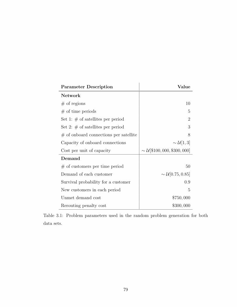
Parameter Description Value

Network

# of regions 10

# of time periods 5

Set 1: # of satellites per period 2

Set 2: # of satellites per period 3

# of onboard connections per satellite 8

Capacity of onboard connections ∼ U [1, 3]

Cost per unit of capacity ∼ U [$100, 000, $300, 000]

Demand

# of customers per time period 50

Demand of each customer ∼ U [0.75, 0.85]

Survival probability for a customer 0.9

New customers in each period 5

Unmet demand cost $750, 000

Rerouting penalty cost $300, 000

Table 3.1: Problem parameters used in the random problem generation for both

data sets.

79

modity l, uses arc (i, j) in time period t and zero otherwise. Additionally, we use

the decision variables ybht that indicate the chosen configuration h, for satellite b,

at time period t. We now present the period-specific capacitated design (PSCAP)

formulation for period t,

(PSCAPt) min∑

l∈L

∑

(i,j)∈At

cltijf

ltij (3.9)

subject to∑

j:(j,i)∈At

f ltji −

∑

j:(i,j)∈At

f ltij = olt

i , ∀t, i ∈ Vt, l ∈ L, (3.10)

∑

l∈L

dltf

ltij ≤ bij, ∀t, (i, j) ∈ At, (3.11)

f ltij −

∑t

∑

b∈Bt

∑

h∈Hb

ζbhij ybh

t ≤ 0, ∀t, (i, j) ∈ At, l ∈ L, (3.12)

∑

h∈Hb

ybht = 1, ∀t, b ∈ Bt, (3.13)

f ltij ∈ {0, 1}, ∀t, l ∈ L, (i, j) ∈ At, (3.14)

ybht ∈ {0, 1} ∀t, b ∈ Bt, h ∈ Hb. (3.15)

where ζbhij is the coefficient we defined earlier in the context of the pricing problem

(see Section 3.4.1) and olti is equal to −1 or 1 if i is the origin node or destination

node of commodity l at time period t, respectively and zero otherwise (as in Section

2.5.1). The only differences between PSRt and PSCAPt are the constraint sets

(3.12), (3.13) and (3.15) which restrict flow only on selected configurations, enforce

the selection of exactly one configuration and define the configuration variables as

binary, respectively. Just like we did in Section 2.5.1 the coefficients cltij are set equal

to cijdlij + el

t (where elt is the rerouting penalty) if commodity l has not used arc

(i, j) in period t− 1 and (i, j) represents an onboard connection. It is important to

80

note that this type of period-by-period model presented here may not be possible

for general problems. Specifically, in the satellite network context the rerouting

penalty is associated with the use of specific arcs in our graph, G. If the penalty

is associated with the entire path, as opposed to the use of a single arc, then the

updating of the cost coefficients cltij would not have been possible and the flow based

model PSCAPt would not have been able to account for the rerouting penalties at

all.

Tables 3.2, 3.3 and 3.4 present a comparison between the BPC procedure and

the period-by-period approach for the three different versions of the first data set.

Each row in the tables present average values over 20 problems for different load

factors, which are specified in the first column. The next two columns present

primal (upper) bounds and computational times (in seconds) for the period-by-

period approach, respectively. The next three refer to the BPC procedure and show

the primal bound achieved, the percentage gap between the primal and dual bounds

and the computational time (in seconds). The last two columns show the average

percentage gap between the primal bounds achieved by the two procedures over all

instances and over the instances that converged, respectively. We allowed the BPC

procedure to run for 1 hour and that is why in some cases the period-by-period

approach has found a better solution. In these cases the average gap between the

primal bounds over all instances assumes a negative value. This is an indication

that the problem becomes harder when we consider more configurations for each

satellite and that the BPC procedure requires more time to provide benefits over a

period-by-period approach. Table 3.2 can serve as a benchmark against which the

81

results in Tables 3.3 and 3.4 can be compared to show the effects of considering

multiple configurations per satellite. Specifically, we see by the increase in average

computation times for both approaches that the problems become harder when more

configurations per satellite are considered. Additionally, the average percentage

gap between the primal solutions for the two approaches also increases for more

configurations. For example if we consider the set in which the load factor is equal

to 0.5 we see the gap increasing from 2.268% for one configuration, to 3.986% for

two configurations, to 4.795% for three configurations. This increase is an indication

of the added benefits of using a BPC procedure as opposed to a period-by-period

approach.

In Tables 3.5, 3.6 and 3.7 we present a comparison between the BPC procedure

and the period-by-period approach for the three different versions of the second

data set. The tables are structured in exactly the same way as before. From the

percentage gaps between the primal solutions we can see that the differences in the

quality of the solutions between the two approaches have increased. This observation

can be attributed to the nature of the second data set that incorporates a much more

dynamic topology. We remind the reader that in this data set only two of the three

satellites are available for use in each time period. This way we are able to replicate

the usual relocations, launches and decommissions of satellites in a typical GEO

network over multiple years. The tables also allow us to draw similar conclusions as

for the first data set. Namely, we can observe that the problems become harder and

that the benefits of using a BPC procedure increase as the number of configurations

for each satellite increases.

82

Loa

dPer

iod-b

y-P

erio

dM

ult

iper

iod

(BP

C)

Pri

mal

Gap

s(%

)

Fac

tor

Pri

mal

($)

Tim

e(s

)P

rim

al($

)G

ap(%

)T

ime

(s)

Ove

rall

Con

verg

ed

0.4

36,9

59,0

180.

2836

,284

,162

0.00

35.1

61.

901.

90

0.5

47,0

39,2

120.

3045

,990

,149

0.00

95.6

90.

062.

27

0.6

61,1

32,4

180.

2759

,982

,060

1.09

1,08

9.60

2.04

3.00

0.7

82,3

43,7

480.

2681

,901

,434

4.10

777.

371.

174.

54

0.8

109,

679,

295

0.25

108,

673,

333

5.11

1,44

2.08

1.40

5.40

Tab

le3.

2:C

ompar

ison

ofPer

iod-b

y-P

erio

dto

Mult

iper

iod

opti

miz

atio

nunder

diff

eren

tlo

ad-fac

tors

for

singl

e-co

nfigu

rati

on

sate

llit

esin

the

firs

tdat

ase

t.

Loa

dPer

iod-b

y-P

erio

dM

ult

iper

iod

(BP

C)

Pri

mal

Gap

s(%

)

Fac

tor

Pri

mal

($)

Tim

e(s

)P

rim

al($

)G

ap(%

)T

ime

(s)

Ove

rall

Con

verg

ed

0.4

33,3

85,8

580.

6132

,408

,128

0.03

732.

663.

063.

09

0.5

44,1

21,5

300.

6742

,449

,194

0.00

447.

040.

383.

99

0.6

59,9

62,9

931.

2862

,022

,157

9.91

1,78

9.69

-1.0

05.

40

0.7

81,0

43,2

120.

7681

,640

,012

7.48

1,48

8.90

0.52

6.51

0.8

109,

054,

991

0.78

125,

896,

228

23.3

92,

345.

66-1

0.68

4.95

Tab

le3.

3:C

ompar

ison

ofPer

iod-b

y-P

erio

dto

Mult

iper

iod

opti

miz

atio

nunder

diff

eren

tlo

ad-fac

tors

for

sate

llit

esw

ith

two

configu

rati

ons

inth

efirs

tdat

ase

t.

83

Loa

dPer

iod-b

y-P

erio

dM

ult

iper

iod

(BP

C)

Pri

mal

Gap

s(%

)

Fac

tor

Pri

mal

($)

Tim

e(s

)P

rim

al($

)G

ap(%

)T

ime

(s)

Ove

rall

Con

verg

ed

0.4

32,6

12,2

731.

0131

,665

,477

0.55

1,13

4.43

3.08

3.68

0.5

43,4

90,9

432.

1343

,062

,039

3.50

947.

120.

384.

80

0.6

57,7

82,5

3020

.06

59,8

03,8

698.

492,

406.

40-1

.69

5.14

0.7

79,7

23,6

6424

.70

95,4

61,2

6428

.86

2,89

1.07

-12.

237.

34

0.8

105,

161,

090

1.66

144,

505,

214

50.6

93,

104.

43-2

3.38

4.47

Tab

le3.

4:C

ompar

ison

ofPer

iod-b

y-P

erio

dto

Mult

iper

iod

opti

miz

atio

nunder

diff

eren

tlo

ad-fac

tors

for

sate

llit

esw

ith

thre

e

configu

rati

ons

inth

efirs

tdat

ase

t.

Loa

dPer

iod-b

y-P

erio

dM

ult

iper

iod

(BP

C)

Pri

mal

Gap

s(%

)

Fac

tor

Pri

mal

($)

Tim

e(s

)P

rim

al($

)G

ap(%

)T

ime

(s)

Ove

rall

Con

verg

ed

0.4

47,7

31,9

340.

3143

,905

,504

0.00

292.

558.

748.

75

0.5

62,8

24,2

190.

2558

,169

,613

0.06

218.

710.

278.

07

0.6

82,3

48,6

310.

2876

,475

,339

0.73

921.

787.

718.

66

0.7

103,

018,

136

0.27

94,9

40,8

850.

3562

5.52

8.53

8.87

0.8

127,

901,

316

0.26

123,

180,

851

4.61

1,59

4.87

4.36

8.56

Tab

le3.

5:C

ompar

ison

ofPer

iod-b

y-P

erio

dto

Mult

iper

iod

opti

miz

atio

nunder

diff

eren

tlo

ad-fac

tors

for

singl

e-co

nfigu

rati

on

sate

llit

esin

the

seco

nd

dat

ase

t.

84

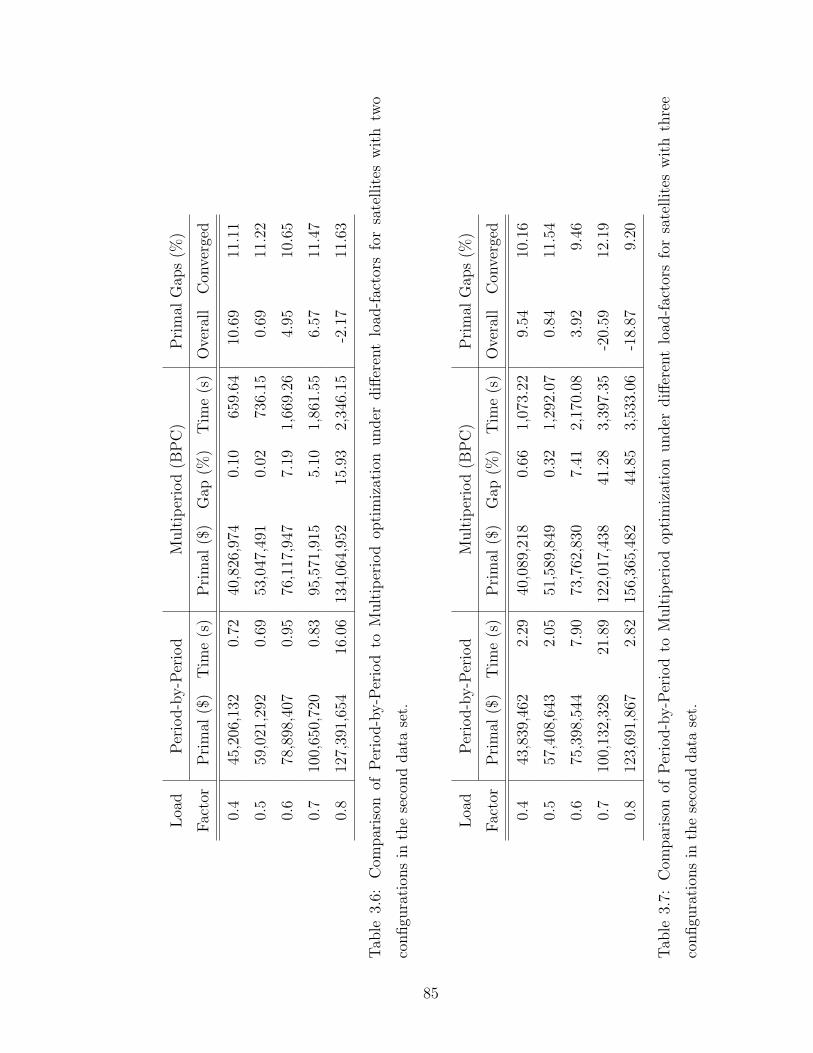
Loa

dPer

iod-b

y-P

erio

dM

ult

iper

iod

(BP

C)

Pri

mal

Gap

s(%

)

Fac

tor

Pri

mal

($)

Tim

e(s

)P

rim

al($

)G

ap(%

)T

ime

(s)

Ove

rall

Con

verg

ed

0.4

45,2

06,1

320.

7240

,826

,974

0.10

659.

6410

.69

11.1

1

0.5

59,0

21,2

920.

6953

,047

,491

0.02

736.

150.

6911

.22

0.6

78,8

98,4

070.

9576

,117

,947

7.19

1,66

9.26

4.95

10.6

5

0.7

100,

650,

720

0.83

95,5

71,9

155.

101,

861.

556.

5711

.47

0.8

127,

391,

654

16.0

613

4,06

4,95

215

.93

2,34

6.15

-2.1

711

.63

Tab

le3.

6:C

ompar

ison

ofPer

iod-b

y-P

erio

dto

Mult

iper

iod

opti

miz

atio

nunder

diff

eren

tlo

ad-fac

tors

for

sate

llit

esw

ith

two

configu

rati

ons

inth

ese

cond

dat

ase

t.

Loa

dPer

iod-b

y-P

erio

dM

ult

iper

iod

(BP

C)

Pri

mal

Gap

s(%

)

Fac

tor

Pri

mal

($)

Tim

e(s

)P

rim

al($

)G

ap(%

)T

ime

(s)

Ove

rall

Con

verg

ed

0.4

43,8

39,4

622.

2940

,089

,218

0.66

1,07

3.22

9.54

10.1

6

0.5

57,4

08,6

432.

0551

,589

,849

0.32

1,29

2.07

0.84

11.5

4

0.6

75,3

98,5

447.

9073

,762

,830

7.41

2,17

0.08

3.92

9.46

0.7

100,

132,

328

21.8

912

2,01

7,43

841

.28

3,39

7.35

-20.

5912

.19

0.8

123,

691,

867

2.82

156,

365,

482

44.8

53,

533.

06-1

8.87

9.20

Tab

le3.

7:C

ompar

ison

ofPer

iod-b

y-P

erio

dto

Mult

iper

iod

opti

miz

atio

nunder

diff

eren

tlo

ad-fac

tors

for

sate

llit

esw

ith

thre

e

configu

rati

ons

inth

ese

cond

dat

ase

t.

85

3.5.2 BPC vs. Root-Node

In this section we compare the BPC procedure with a Root-Node procedure

for the two data sets that we have generated. In Tables 3.8, 3.9 and 3.10 we present

the results for the first data set. These tables present primal solutions, percentage

gaps between primal and dual bounds and computational times (in seconds) for

both procedures. They also show the percentage gaps between the primal solutions

reached by the two approaches in the allotted time frame (1 hour) over all instances

and over the instances that converged. In Table 3.8 we see that the Root-Node

procedure gives results that are very close to the results of the BPC approach,

which is exactly what we had observed in Chapter 2. However, in Tables 3.9 and

3.10 we see a very significant difference between the two approaches. What is more

is the fact that based on the earlier comparison between BPC and period-by-period

we can draw the conclusion that that the period-by-period approach outperforms

the Root-Node approach for most cases in which there are multiple configurations.

One possible explanation for this could be the fact that the Root-Node procedure

generates enough columns to find the optimal solution at the root node of the tree

but these columns might not include paths in some of the configurations that are in

the optimal solution.

Tables 3.11, 3.12 and 3.13 show the results for the BPC and Root-Node ap-

proaches for the second data set. Once again we observe that in the first table

the two procedures are comparable while in the remaining two the BPC approach

is clearly better by very large margins. Additionally, similar to our observations in

86

Chapter 2, the solutions of the BPC algorithm contain paths with significantly fewer

rerouting penalties which helps to explain the improvements seen in the objective

value comparisons.

87

Loa

dR

oot

-Node

BP

CP

rim

alG

ap(%

)

Fac

tor

Pri

mal

($)

Gap

(%)

Tim

e(s

)P

rim

al($

)G

ap(%

)T

ime

(s)

Ove

rall

Con

verg

ed

0.4

36,2

84,1

620.

001.

9236

,284

,162

0.00

35.1

60.

000.

00

0.5

45,9

91,9

410.

004.

5145

,990

,149

0.00

95.6

90.

000.

00

0.6

59,8

85,0

520.

9062

2.65

59,9

82,0

601.

091,

089.

60-0

.16

0.03

0.7

78,7

86,5

900.

0012

2.39

81,9

01,4

344.

1077

7.37

-3.2

60.

05

0.8

105,

064,

629

0.98

302.

3510

8,67

3,33

35.

111,

442.

08-2

.98

0.21

Tab

le3.

8:C

ompar

ison

ofth

eR

oot

-Node

appro

ach

toth

eB

PC

pro

cedure

for

sate

llit

esw

ith

asi

ngl

eco

nfigu

rati

onin

the

firs

t

dat

ase

t.

Loa

dR

oot

-Node

BP

CP

rim

alG

ap(%

)

Fac

tor

Pri

mal

($)

Gap

(%)

Tim

e(s

)P

rim

al($

)G

ap(%

)T

ime

(s)

Ove

rall

Con

verg

ed

0.4

33,6

25,6

980.

0320

0.26

32,4

08,1

280.

0373

2.66

3.65

3.51

0.5

47,2

60,8

580.

0022

.83

42,4

49,1

940.

0044

7.04

11.4

411

.44

0.6

68,1

22,7

192.

6022

6.53

62,0

22,1

579.

911,

789.

6912

.45

16.5

8

0.7

88,2

98,3

120.

0029

.79

81,6

40,0

127.

481,

488.

909.

3614

.45

0.8

116,

964,

373

0.03

35.6

812

5,89

6,22

823

.39

2,34

5.66

-4.3

011

.65

Tab

le3.

9:C

ompar

ison

ofth

eR

oot

-Node

appro

ach

toth

eB

PC

pro

cedure

for

sate

llit

esw

ith

two

configu

rati

ons

inth

efirs

tdat

a

set.

88

Loa

dR

oot

-Node

BP

CP

rim

alG

ap(%

)

Fac

tor

Pri

mal

($)

Gap

(%)

Tim

e(s

)P

rim

al($

)G

ap(%

)T

ime

(s)

Ove

rall

Con

verg

ed

0.4

34,2

50,1

300.

0016

.77

31,6

65,4

770.

551,

134.

438.

058.

84

0.5

50,4

57,8

940.

0021

.29

43,0

62,0

393.

5094

7.12

18.3

421

.37

0.6

71,2

38,8

930.

1133

6.25

59,8

03,8

698.

492,

406.

4020

.87

23.5

7

0.7

101,

716,

588

2.39

242.

6795

,461

,264

28.8

62,

891.

0710

.98

32.0

6

0.8

128,

469,

498

0.00

81.5

614

4,50

5,21

450

.69

3,10

4.43

-6.9

922

.98

Tab

le3.

10:

Com

par

ison

ofth

eR

oot

-Node

appro

ach

toth

eB

PC

pro

cedure

for

sate

llit

esw

ith

thre

eco

nfigu

rati

ons

inth

efirs

t

dat

ase

t.

Loa

dR

oot

-Node

BP

CP

rim

alG

ap(%

)

Fac

tor

Pri

mal

($)

Gap

(%)

Tim

e(s

)P

rim

al($

)G

ap(%

)T

ime

(s)

Ove

rall

Con

verg

ed

0.4

43,9

53,7

660.

0011

.07

43,9

05,5

040.

0029

2.55

0.11

0.12

0.5

58,1

54,5

640.

0041

.92

58,1

69,6

130.

0621

8.71

-0.0

30.

00

0.6

75,9

59,1

080.

0128

0.14

76,4

75,3

390.

7392

1.78

-0.6

20.

03

0.7

94,6

60,1

860.

0010

1.05

94,9

40,8

850.

3562

5.52

-0.2

70.

06

0.8

120,

854,

403

2.23

757.

5512

3,18

0,85

14.

611,

594.

87-1

.61

0.28

Tab

le3.

11:

Com

par

ison

ofth

eR

oot

-Node

appro

ach

toth

eB

PC

pro

cedure

forsa

tellit

esw

ith

asi

ngl

eco

nfigu

rati

onin

the

seco

nd

dat

ase

t.

89

Loa

dR

oot

-Node

BP

CP

rim

alG

ap(%

)

Fac

tor

Pri

mal

($)

Gap

(%)

Tim

e(s

)P

rim

al($

)G

ap(%

)T

ime

(s)

Ove

rall

Con

verg

ed

0.4

45,5

42,7

350.

0115

4.91

40,8

26,9

740.

1065

9.64

11.5

811

.47

0.5

61,4

27,9

590.

0026

.63

53,0

47,4

910.

0273

6.15

15.9

315

.64

0.6

86,1

37,2

431.

4628

3.14

76,1

17,9

477.

191,

669.

2614

.37

18.6

9

0.7

108,

665,

879

0.00

34.9

295

,571

,915

5.10

1,86

1.55

15.2

920

.54

0.8

130,

223,

649

0.00

213.

1813

4,06

4,95

215

.93

2,34

6.15

-0.2

911

.87

Tab

le3.

12:

Com

par

ison

ofth

eR

oot

-Node

appro

ach

toth

eB

PC

pro

cedure

for

sate

llit

esw

ith

two

configu

rati

ons

inth

ese

cond

dat

ase

t.

Loa

dR

oot

-Node

BP

CP

rim

alG

ap(%

)

Fac

tor

Pri

mal

($)

Gap

(%)

Tim

e(s

)P

rim

al($

)G

ap(%

)T

ime

(s)

Ove

rall

Con

verg

ed

0.4

46,6

93,5

210.

0036

.40

40,0

89,2

180.

661,

073.

2216

.81

17.3

1

0.5

64,4

47,9

850.

0053

.49

51,5

89,8

490.

321,

292.

0725

.06

23.9

5

0.6

90,3

26,2

050.

0076

.65

73,7

62,8

307.

412,

170.

0824

.31

30.2

1

0.7

116,

845,

336

0.00

65.5

012

2,01

7,43

841

.28

3,39

7.35

-7.6

025

.09

0.8

139,

848,

680

0.00

125.

8815

6,36

5,48

244

.85

3,53

3.06

-8.5

724

.28

Tab

le3.

13:

Com

par

ison

ofth

eR

oot

-Node

appro

ach

toth

eB

PC

pro

cedure

for

sate

llit

esw

ith

thre

eco

nfigu

rati

ons

inth

ese

cond

dat

ase

t.

90

3.5.3 Integer vs. Linear Configuration Variables

In order to explore the effect of the configuration variables on the BPC pro-

cedure we solved the problems that had satellites with two configurations in the

first data set with linear as well as integer configuration variables. In Table 3.14

we present the results of this comparison. The table shows average results for the

percentage gap between the primal and dual bounds, the computation time (in sec-

onds), the number of nodes in the BPC tree and the number of columns and cuts

added during both approaches. The last column presents the percentage gap of the

primal solutions reached after 1 hour. By looking at the average number of nodes

generated by the two approaches we see that when the configuration variables are

binary the BPC tree is generally much smaller. Additionally, the number of columns

and cuts generated with this approach is significantly smaller for the problem sets

with 0.4 and 0.5 load factors. Moreover, the feasible solutions attained within 1

hour when the configuration variables are integer are significantly better (i.e., 12%

for a load factor of 0.4 and more than 40% for load factors 0.5 and 0.6). The signif-

icant differences that are observed can be attributed to the branching mechanism

for integer configuration variables. Specifically, when branching on a configuration

variable we are able to delete large sets of arcs from our graph, G that correspond

to the configurations that are excluded by the branch we are currently on. This

in turn results in the generation of fewer columns and cuts and the exploration of

fewer nodes. In the linear case however this mechanism is absent and as a result we

explore many more nodes and generate more columns and cuts.

91

Loa

dIn

tege

rC

onfigu

rati

onV

aria

ble

sLin

ear

Con

figu

rati

onV

aria

ble

sP

rim

al

Fac

tor

Gap

(%)

Tim

e(s

)N

odes

Col

um

ns

Cuts

Gap

(%)

Tim

e(s

)N

odes

Col

um

ns

Cuts

Gap

(%)

0.4

0.03

732.

798

1.9

2,78

7.6

1,74

0.3

16.8

73,

150.

62,

590.

210

,153

.64,

587.

712

.58

0.5

0.00

447.

049

5.4

3,04

3.7

926.

440

.29

3,60

1.8

2,79

0.4

12,2

76.9

3,73

6.5

30.4

8

0.6

9.91

1,78

9.7

2,07

9.8

10,4

42.8

4,69

0.5

78.6

23,

601.

42,

324.

212

,002

.04,

016.

348

.09

0.7

7.48

1,48

8.9

1,34

2.5

12,3

49.0

3,81

5.9

75.7

93,

601.

32,

399.

312

,970

.35,

077.

143

.96

Tab

le3.

14:

Com

par

ison

ofin

tege

rvs.

linea

rco

nfigu

rati

onva

riab

les

for

sate

llit

esw

ith

two

configu

rati

ons

inth

efirs

tdat

ase

t.

92

3.6 Concluding Remarks

In this chapter we extended the multiperiod traffic routing problem in con-

sidering alternative configurations of the satellites. Effectively we have defined a

multiperiod capacitated network design (MPCAP) problem which in the context

of satellite networks expresses a multiperiod traffic routing problem with onboard

configuration decisions. We were able to extend the BPC procedure developed in

Chapter 2 to deal with new decision variables that capture the configuration choices.

The main challenges included dealing with the dual variables of the new constraints

associated with the selection of a configuration. We presented two approaches that

can deal with these new variables. The first uses the results developed in Chapter

2 whereas the second one presents a new approach that can deal with rerouting

penalties in much more general settings.

Our computational analysis focused on the impact of including configuration

decisions in satellite planning. We compared the BPC, Root-Node and period-

by-period approaches for problems which included satellites with one, two and

three configurations. Our results indicate that the BPC optimization algorithm

can achieve savings of up to 12% over the period-by-period approach and up to 32%

over the Root-Node approach. These results show that a multiperiod approach can

still add significant value as opposed to a period-by-period process and that the

Root-Node approach does very poorly when multiple configurations or equivalently

network design decisions are involved.

In the satellite problem context that motivated the MPCAP problem there

93

were no costs associated with switching from one configuration to another. However,

in the more general situation in which there is some cost associated with the design

variables (that is also present in the objective function) we would need to revise

our solution approach. Specifically, the main question that needs to be explored

is whether the design variables should also be decoupled from the time dimension

subscript. This would mean that we would have to define configuration paths for

each satellite that would specify the configuration that each satellite would use for all

time periods. Naturally, this would lead to an exponential number of configuration

variables and an associated pricing problem. This approach introduces many new

challenges that have to do with the generation of two different types of columns

for the solution of each restricted LP as well as branching and initial feasibility

considerations. We leave this for future research and note that Stanojevic [78]

discusses aspects of column generation with two different types of (exponentially

sized) variables in the context of optical network design.

94

Chapter 4

Multiperiod Traffic Routing with Uncertain Demand

4.1 Problem Definition

In this chapter we approach the MPTR problem but we assume that future

customer demands are not known with certainty. Specifically, we assume that the

network planners are still able to forecast individual traffic demands with reason-

able accuracy but the actual demands that will occur depend on prevailing market

conditions. The reasoning behind this assumption is that even though expected

demands for individual customers are forecasted it would be virtually impossible to

define separate probability distributions for all of them. However, it is more rea-

sonable to analyze the prevailing market trends for different services and between

different regions and come up with specific distributions for the possible realizations

of these trends. Additionally, we assume that demands for the first time period are

known with certainty while demands for the remaining time periods are the ones

for which we are uncertain. In the stochastic multiperiod traffic routing problem

(SMPTR) we wish to minimize the expected traffic routing costs over all random

scenarios while routing service requests with uncertain demand over a given satellite

network for multiple time periods. We will also extend our work to the stochastic

multistage capacitated network design problem (SMCAP) and comment on solution

methodologies for stochastic multicommodity flow and integer stochastic programs

95

in general.

4.2 Related Literature

The practice of introducing uncertainty into problems and making decisions

based on probability distributions of unknown events adds significant value to the

resulting Stochastic Programming (SP) models. For a good introduction to the field

of stochastic optimization see Ruszczynski and Shapiro [70], Birge and Louveaux

[19] and Kall and Wallace [49].

There have been several papers in the literature that deal with network plan-

ning and design decisions with uncertain demand in a telecommunications and other

contexts. Sen et al. [74] define a two-stage problem where the first-stage decision

variables correspond to the installation of capacity on the edges of a network and

the second stage decision variables deal with routing demand between origins and

destinations. The objective in that problem is to minimize unmet demand. Riis

and Andersen [68] discuss the same problem and develop a procedure based on an

L-Shaped algorithm. They discuss and use various families of cuts and test their

approach on real-life instances but their objective is to minimize the expected cost

of installing the new facilities and routing the traffic. Medova [61] looks at traffic

routing of a telecommunications network with uncertain demands over a single stage

and formulates a multicommodity flow model with chance-constraints, where flow

splitting is allowed. Smith et al. [77] look at a two-stage stochastic problem that

involves the installation of add-drop multiplexors on SONET rings and solve it with

96

an L-Shaped method.

A somewhat related problem that has attracted a lot of attention in the liter-

ature is the capacity expansion problem. Even though capacity expansion problems

have been motivated by facility installation in the telecommunications and other

industries their defining characteristic that sets them apart from network design

problems is that typically they involve decisions on capacity installation but not

routing. Riis and Lodahl [69] formulate a bicriteria capacity expansion problem in

which both the total expected capacity cost and the probability of violating future

capacity restrictions is minimized. Saniee [71] looks at a multistage capacity ex-

pansion problem of a single location and develops a very efficient technique to solve

it. Riis and Andersen [67] discuss a preprocessing rule and a new formulation for

a multistage capacity expansion problem of a single communications link. More

recently, Ahmed and Sahinidis [2] look at a general multistage integer capacity ex-

pansion problem under uncertainty and develop an approximation algorithm which

they test on different types of chemical process networks for different numbers of

time periods. Also, Ahmed et al. [1] developed an exact approach that successfully

deals with an integer multistage capacity expansion problem.

Another well studied stochastic problem is the stochastic transportation prob-

lem (STP). This problem requires the transportation of commodities from a set of

supply points to a set of demand points and typically assumes that the demands

are uncertain. The STP is usually modeled on bipartite graphs and does not in-

volve general networks, routing decisions or multicommodity flow like some of the

network design and planning problems discussed previously. For a nice review of

97

several papers on STP and various decomposition techniques see Holmberg [44].

The majority of the stochastic programming literature that deals with two-

stage or multistage recourse problems treats cases in which the programs are linear.

For these types of problems several procedures have been developed over the years.

The most prominent of these approaches is the outer linearization or more commonly

known as the L-Shaped method introduced by Van Slyke and Wets [76] which is based

on Benders decomposition [14]. A related procedure, but not as popular, is the so-

called inner linearization, which was first suggested by Dantzig and Madansky [28]

for solving stochastic problems.

On the other hand, there have been significantly fewer approaches for general

problems that contain integer (or binary) variables, especially if these are present at

any of the later stages in a stochastic program. The first extension of the L-Shaped

method for a two-stage problem with binary first and second stage was presented by

Laporte and Louveaux [53]. Unfortunately their method only works for cases where

the first-stage variables are continuous. Carøe and Tind [23] extended the L-Shaped

method for mixed-integer first and second stage variables. Carøe and Schultz [22]

develop a method for multistage integer recourse problems that is based on what

is known as variable splitting or Lagrangian Decomposition. They comment on the

fact that implementation for multiple stages can become computationally expensive

and present results on a two-stage problem. Schultz et al. [73] develop a procedure

for integer stochastic programs in which they exploit the similarity in structure

between the scenario dependent integer problems by using a Grobner basis strategy.

Klein Haneveld et al. [41, 42] present a solution procedure for a class of two-stage

98

integer stochastic programs that have a special structure known as simple recourse.

Their approach constructs an envelope for the second-stage value function. Recently,

Ahmed et al. [3] present a branch-and-bound algorithm for a two-stage stochastic

program with mixed-integer first-stage variables and integer second-stage variables.

They propose a variable reformulation, an associated branching strategy and bound

calculation for the second stage value function and provide computational results.

The papers by Ahmed et al. [1, 2] discussed earlier in the context of capacity

expansion also deal with integer stochastic programs. For a fairly recent review of

the different approaches developed for integer stochastic programs see the paper by

Klein Haneveld and van der Vlerk [43].

From the brief review of the most prominent approaches for stochastic pro-

grams with integer recourse it should be clear that very few procedures can deal

with integer stochastic programs without significant assumptions on the structure

of these problems and even fewer can be generalized for multistage problems in which

integer variables exist at all stages. In this chapter we will present a branch-and-

price approach that can be applied to multistage stochastic multicommodity flow

problems with integer variables at all stages. More importantly our approach can

inherently deal with an arbitrary number of stages and the inclusion of additional

stages involves only a limited computational penalty. To the best of our knowledge

the use of the Dantzig-Wolfe decomposition principle on an appropriate reformu-

lation of the primal problem has never been used to solve stochastic multistage

recourse problems with integer variables at all stages.

99

4.3 Problem Formulations

In this section we will present the nature of uncertainty in future service re-

quests and model the SMPTR problem on exactly the same graph as the one we

used in Chapter 2. We also introduce two stochastic programming models. The

first one is based on a multicommodity flow approach while the second one uses the

notion of super-paths introduced in Chapter 2.

4.3.1 Uncertainty

We model the SMPTR problem under the assumption that demand dlt for

each commodity l and each time period t, except the first, is uncertain. In order

to account for uncertainty, we let the demand be dependent on the outcome of a

random variable ξ. Naturally, our problem can be viewed as a multistage recourse

problem where the routing of the demand has to be determined at each period

(stage). Routing for current demand (time period 1) can be determined in the first

stage with certainty, since the actual demand is known (customers have expressed

their requirements). However, the routing of future time period demands has to be

decided when it is realized. Those later decisions will undoubtedly suffer (or benefit)

by rerouting penalties (or their absence) that result from the decisions taken in the

previous period (stage). We denote the dependence of the demand of commodity l,

at time period t on ξ as dlt(ξ).

We assume that the random variable ξ has a discrete distribution with finite

support, say Ξ = {ξs : s ∈ S} and corresponding probabilities P (ξ = ξs) = qs,

100

for all s ∈ S. Notice that the realization of a scenario s for the random variable ξ

will determine the demand dlt(ξ

s) for all time periods t in the time horizon and all

customers l. For notational convenience we will denote the demand for customer l,

in time period t, under scenario s, as dlst . This notion of scenarios and the definition

of ξ is quite common in stochastic programming (see [19, 70] for various examples).

The scenarios are typically represented as part of a scenario tree with a single root

node and multiple branches. Each path in this tree, from the root to each leaf

node represents a scenario. In Figure 4.1 we present a simple scenario tree with six

scenarios and three time periods. Since there is a unique path from the root node to

a leaf node, for brevity we label the leaf node with the scenario number. Each node

n in the scenario tree is associated with a set of scenarios Sn that can occur from

that node. Also, for each period t, let Bt include all sets Sj such that node j is in

period t. For example in Figure 4.1 S2 = {1, 2, 3}, S3 = {4, 5, 6} and B2 = {S2,S3}.

In practice our approach could be used by planners at the start of a plan-

ning period to make decisions on the routing of existing requests (i.e., known with

certainty) for the upcoming time period. Even though this optimization run pro-

vides decisions for all customers over all the time periods and under all scenarios

the planners will re-optimize at the start of each period. Each subsequent run uses

new information for new customers that want to receive service and future scenar-

ios. Once again the results for these runs will provide planners with the routing

decisions that have to be taken in the current time period. In this way the network

planners always make decisions based on the most recent information while also

taking into account the probability of future events that can potentially have an

101

4

5

6

7

8

9

t = 1 t = 2 t = 3

s = 1

s = 2

s = 3

s = 4

s = 5

s = 6

1

2

3

Root

Node

Figure 4.1: A small scenario tree for a three-stage (period) problem with six scenar-

ios.

102

effect on current decisions.

4.3.2 Flow Based Model

We use the decision variables f ltij that are equal to 1 when commodity l is using

arc (i, j), at time period t and 0 otherwise. We also introduce the decision variables

zlt that will capture the possible rerouting of commodity l, at time period t. Notice

that both these variables depend on the realization ξs of the random variable ξ. We

denote this dependency as f ltij(ξ

s) and zlt(ξ

s) but for convenience we will instead use

the notation f ltsij and zls

t , respectively. The stochastic multiperiod traffic routing

(SMPTR) problem can now be stated as,

(SMPTR-F) min∑

l∈L

∑

(i,j)∈A1

dl1cijf

l1ij +

T∑t=2

Qt(f t−1) (4.1)

subject to∑

j:(j,i)∈A1

f l1ji −

∑

j:(i,j)∈A1

f l1ij = ol1

i , ∀i ∈ N1, l ∈ L (4.2)

∑

l∈L

dltf

l1ij ≤ bij, ∀(i, j) ∈ A1, (4.3)

f l1ij ∈ {0, 1}, ∀l ∈ L, (i, j) ∈ A1, (4.4)

where the value functions Qt(f t−1) for the different stages in (4.1) depend on the

flow variables in the previous time period. The coefficients ol1i are equal to −1 and 1

when i is the origin and destination of customer l respectively and zero other wise.

The value function Qt(f t−1) is given by the following model,

(SMPTRt) Qt(f t−1) = min qs∑s∈S

∑

l∈L

∑

(i,j)∈At

dlst cijf

ltsij +

∑

l∈L

eltz

ls

(4.5)

103

subject to

∑

j:(j,i)∈At

f ltsji −

∑

j:(i,j)∈At

f ltsij = olt

i ∀i ∈ Nt, s ∈ Sl ∈ L (4.6)

∑

l∈L

dlst f lts

ij ≤ bij, ∀s ∈ S, (i, j) ∈ At, (4.7)

zls − f ltsij + f

l(t−1)sij ≥ 0, ∀(i, j) ∈ Dt, s ∈ S, l ∈ L, (4.8)

zls − fl(t−1)sij − f lts

ij ≥ 0, ∀(i, j) ∈ Dt, s ∈ S, l ∈ L, (4.9)

f lts1ij = f lts2

ij , (s1, s2) ∈ S,S ∈ Bt, l ∈ L, (i, j) ∈ At,(4.10)

f ltsij ∈ {0, 1}, ∀s ∈ S, l ∈ L, (i, j) ∈ At, (4.11)

zls ∈ {0, 1}, ∀s ∈ S, l ∈ L. (4.12)

The SMPTR-F formulation for the first stage problem is a typical multicom-

modity flow formulation with flow conservation (4.2) and capacity restrictions (4.3).

The objective function (4.1) contains the routing costs for the first time period and

the functions Q(f t−1) for the remaining time periods and all scenario realizations.

The SMPTRt formulation gives the t-stage problem over all realizations ξs of the

random variable ξ and the routing decisions made in the previous stage fl(t−1)sij .

The set Dt consists of arcs that belong in At and represent the communication links

onboard the satellites (i.e., the transponders). The objective function of this formu-

lation (4.5) computes the expected routing costs and expected rerouting penalties for

a given time period t and over all scenarios s. Also, it consists of flow conservation

constraints (4.6) and capacity constraints (4.7) but in addition includes constraint

sets (4.8) and (4.9) that capture the rerouting penalties. Specifically, constraints

(4.8) and (4.9) capture the relation |f ltsij −f

l(t−1)sij | = zls in a linear manner. At time

period t if scenarios s1 and s2 are associated with the same node in the scenario

104

tree (i.e., s1, s2 ∈ Sn) then the decisions associated with both scenarios up until

time t have to be exactly the same. In stochastic programming this is referred to

as nonanticipativity (see [19, 70]) and in our model it is ensured by constraint set

(4.10).

4.3.3 Path Based Model

A different way to state the stochastic problem is with the use of the super-

path variables xlp. These variables will also depend on the realization ξs of the

random variable ξ and for convenience we denote them as xlsp . Essentially, xls

p is the

super-path p selected to carry the demand for commodity l under the realization ξs.

We now state the SMPTR problem with the use of the path variables, xlsp .

(SMPTR-P) min∑s∈S

∑

l∈L

∑

p∈P l

qsclsp xls

p (4.13)

subject to

∑

l∈L

∑

p∈P l

dlst δp

ijxlsp ≤ bij, ∀t, s ∈ S, (i, j) ∈ At, (4.14)

∑

p∈P l

xlsp = 1, ∀s ∈ S, l ∈ L, (4.15)

∑

p∈P l

δpijx

lςp −

∑

p∈P l

δpijx

lsp ≥ 0, ∀t, s ∈ S\{ς},S ∈ Bt, l ∈ L, (i, j) ∈ At,(4.16)

xlsp ∈ {0, 1}, ∀s ∈ S, l ∈ L, p ∈ P l. (4.17)

Constraint set (4.14) ensures that capacity restrictions are not violated while

constraint set (4.15) forces the selection of exactly one path for each commodity

l and each scenario s. The difference between the SMPTR-P formulation and the

105

deterministic MPTR formulation (see Section 2.3) is constraint set (4.16). These

constraints enforce nonanticipativity in the path based model in the same way that

constraint set (4.10) did for the arc-flow model. ς is an arbitrary element of set S,

which in turn belongs to set Bt at time period t. Typically, in two-stage or multistage

recourse formulations first stage variables are not dependent on any random variable

and therefore nonanticipativity constraints are not required in the first stage. How-

ever, in our case the super-path variables used define the routes that commodities

will take across the entire planning horizon and therefore define routes for the first

time period or equivalently first stage as well. As a result, we need to make sure

that the first time period paths are the same under any realization of the random

variable. Constraint (4.16), for t = 1, ensures that for each commodity l the super-

paths that will be selected for all scenarios s will share the same first-stage path in

the following way. When xlςp is zero then for all arcs (i, j) that belong to path p the

first term of (4.16) becomes zero. As a result, all variables xlsp , for s ∈ S\{ς} will

be forced to be zero. Alternatively, if xlςp is one, the variables xls

p that correspond to

paths that use the same arc (i, j) as p can be selected. Notice that constraint (4.16)

differs from (4.10) in two ways. First, (4.16) refers to an arbitrary element, ς of S

and compares that to the rest of the scenarios in S, as opposed to comparing pairs

of scenarios (s1, s2) ∈ S. The second difference is that in (4.16) we used a greater-

than-or-equal sign instead of an equal sign. Both of these differences result from the

fact that during the BPC approach that uses the path-based model we will be using

a reduced model that does not contain all possible columns. So, if for any scenario

s ∈ S\{ς} our reduced model didn’t include any columns for the second term then

106

the first term,∑

p∈P l δpijx

lςp , would have been forced to zero which could lead to an

unwanted infeasibility. In exactly the same way, constraint (4.16) ensures, for all

remaining time periods t = {2, . . . , T}, that the decisions taken for two different

scenarios that are associated with the same node in time period t in the scenario

tree are going to be the same up to time t and therefore ensures nonanticipativity.

The SMPTR-P formulation has a very compact objective function but it still

captures all the routing costs and rerouting penalties for all scenarios. Equation

(4.18) presents the objective (4.13) in an extensive form. With the help of equa-

tion (2.4) we can substitute (4.18) with the compact form found in the SMPTR-P

formulation.

∑s∈S

qs∑

t

∑

l∈L

∑

p∈P l

∑

(i,j)∈At

dlst cijδ

pijx

lsp + el

tγpt x

lsp

(4.18)

4.4 Solution Approach

In this section we outline two solution approaches for each of our stochastic

programming models. The first is the traditional L-Shaped algorithm for the flow

based SMPTR-F model and the second is a branch-and-price-and-cut (BPC) ap-

proach for the SMPTR-P model. Note, that a BPC approach is a novel way to deal

with a multistage stochastic integer problem that has never been used before.

107

4.4.1 L-Shaped Algorithm

To simplify the presentation of our L-Shaped algorithm we provide a brief

overview of the general steps taken during the L-Shaped method for a two stage

linear stochastic program.

Overview

When the random vector ξ has finite support then it is possible to write the

associated problem in extensive form. In this form we associate one set of decision

variables, say Yst , with each scenario s and stage t (exactly as we have done for

the SMPTR-F model). In this extensive form the problems have a block angular

structure which we wish to exploit. For example a two-stage recourse problem in

extensive form will have the following structure,

A1

A21 W

A22 . . . W

.... . .

A2s . . . . . . W

.... . .

where A1 is the matrix associated with the first stage decisions and A2s is the matrix

associated with the first stage variables under realization (scenario) s. W is a matrix

associated with second stage decisions for all realizations of the random variable ξ.

The Benders decomposition principle can be used to take advantage of such a form.

108

In practice, the typical Benders method is extended to what is known as the L-

Shaped method that takes care of feasibility concerns in the context of stochastic

programs. During the L-Shaped method (see Figure 4.2) we solve a master problem

that involves all first-stage decisions and any cuts we add during the procedure.

The objective of this master problem includes all terms associated with first-stage

variables and an auxiliary real variable, say ϑ. Once we solve the master problem we

need to check whether this solution is feasible under all realizations of the random

variable and add appropriate constraints in case it is not. We do this with the use of a

feasibility subproblem that either declares the current optimal solution of the master

problem as feasible or determines an appropriate cut that needs to be added to the

master problem to get a feasible solution. There is one feasibility subproblem for

each scenario and each one consists of auxiliary terms in the objective function and

the constraint set associated with the specific scenario realization. Once we find an

optimal solution to the master problem that is also feasible under the realizations of

the random variable we solve an optimality subproblem. The optimality subproblem

either declares our solution to be optimal or determines an appropriate cut that when

added to the master problem will improve the objective of the master. There is one

optimality subproblem for each scenario and each one consists of the constraint set

and objective function terms associated with that specific scenario. In the following

section we define the master and both subproblems for the SMPTR problem.

109

Begin

Step 0: Solve master problem

Step 1: for s = 1, . . . , |S| do

Solve feasibility subproblem (FEASs)

end for

if there are any feasibility cuts add them to the master problem,

and go to Step 0.

Step 2: for s = 1, . . . , |S| do

Solve optimality subproblem (OPTs)

end for

if there are any optimality cuts add them to the master problem,

and go to Step 0.

End

Figure 4.2: L-Shaped algorithm.

110

4.4.2 Master Problem, Feasibility and Optimality Cuts

We will first derive the cuts required for an L-Shaped algorithm for the linear

relaxation of a two-stage traffic routing problem and then make comments on gener-

alizations to multiple stages and integer variables. The standard L-Shaped method

requires that we solve the following master problem,

(L-MASTER) min∑

l∈L

∑

(i,j)∈A1

dl1cijf

l1ij + ϑ

subject to∑

j:(j,i)∈A1

f l1ji −

∑

j:(i,j)∈A1

f l1ij = ol1

i ∀i ∈ N1, l ∈ L, (4.19)

∑

l∈L

dltf

l1ij ≤ bij, ∀(i, j) ∈ A1, (4.20)

∑

l∈L

∑

(i,j)∈D1

M lrij f

l1ij ≥ dl, ∀r = 1, . . . , RF , (4.21)

∑

l∈L

∑

(i,j)∈D1

N lrij f

l1ij + ϑ ≥ gl, ∀r = 1, . . . , RO, (4.22)

f l1ij ∈ [0, 1], ∀l ∈ L, (i, j) ∈ A1, (4.23)

ϑ ∈ R. (4.24)

Constraints (4.19) and (4.20) are the typical flow conservation and capacity

restriction constraints, respectively. Constraint set (4.21) defines a set {1, . . . , RF}

of feasibility constraints while constraint set (4.22) defines the set {1, . . . , RO} of

optimality constraints. M lrij and N lr

ij are the coefficients of the feasibility and opti-

mality cuts respectively that will be computed during the iterations of the L-Shaped

algorithm.

If we look at the way the feasibility cuts are generated then we see that for

each scenario s we need to solve the linear program,

111

(FEASs) min∑

l∈L

∑

(i,j)∈A

(vl1ij + vl2

ij ) (4.25)

subject to∑

j:(j,i)∈A2

f l2sji −

∑

j:(i,j)∈A2

f l2sij = ol2

i ∀i ∈ N2, l ∈ L (4.26)

∑

l∈L

dls2 f l2s

ij ≤ bij, ∀(i, j) ∈ A2, (4.27)

−f l1ij + f l2s

ij + zls + vl1ij ≥ 0, ∀(i, j) ∈ D2, l ∈ L, (4.28)

f l1ij − f l2s

ij + zls + vl2ij ≥ 0, ∀(i, j) ∈ D2, l ∈ L, (4.29)

f l2ij ∈ [0, 1], ∀l ∈ L, (i, j) ∈ A2, (4.30)

zls ∈ [0, 1], ∀l ∈ L, (4.31)

vl1ij , v

l2ij ≥ 0 ∀l ∈ L, (i, j) ∈ A2. (4.32)

vl1ij and vl2

ij are auxiliary variables that will help us compute the necessary feasibility

cuts that we need to add to the L-MASTER model. If for some scenario s and the

selected first-stage variables f l1ij the objective of FEASs is strictly positive we need

to add the following feasibility cut to the master problem,

∑

l∈L

∑

(i,j)∈B1

(ηlsij − λls

ij)fl1ij ≥ 0

where ηlsij and λls

ij are the dual variables of constraints (4.28) and (4.29) in FEASs,

respectively. Note that sets D1 and D2 consist of arcs in A1 and A2 that represent

the same onboard connections in both time periods. The cut guarantees that f l1ij ∈

K2(ξ), where K2(ξ) is the set of first-stage variables for which the second stage

problems, under all random realizations of ξ are feasible. However, based on the

augmentations we have made on the graph G we can guarantee that the second

stage problem will always be feasible, under all scenarios s and first stage decisions

112

f l1ij . Specifically, the unmet arcs (i, j) that we have introduced in At, for all t and

for each commodity l between the origin and destination of that commodity (see

Section 2.4), ensure feasibility. As a result of these augmentations the auxiliary

variables in FEASs will always be equal to zero and we will never have to generate

feasibility cuts.

In order to generate the optimality cuts (4.22) we need to solve the following

linear program for each scenario s,

(OPTs) min∑

l∈L

∑

(i,j)∈A2

cijfl2sij +

∑

l∈L

el2z

ls2 (4.33)

subject to∑

j:(j,i)∈A2

f l2sji −

∑

j:(i,j)∈A2

f l2sij = ol2

i ∀i ∈ N2, l ∈ L, (4.34)

∑

l∈L

dls2 f l2s

ij ≤ bij, ∀(i, j) ∈ A2, (4.35)

−f l1ij + f l2s

ij + zls ≥ 0, ∀(i, j) ∈ D2, l ∈ L, (4.36)

f l1ij − f l2s

ij + zls ≥ 0, ∀(i, j) ∈ D2, l ∈ L, (4.37)

f l2ij ∈ [0, 1] ∀l ∈ L, (i, j) ∈ A2, (4.38)

zls ∈ [0, 1] ∀l ∈ L. (4.39)

Once we solve OPTs for all s ∈ S we can check whether the current first-stage

variables satisfy the following condition.

∑

k∈K

∑

(i,j)∈B2

(∑s∈S

qs(κksij − µks

ij )

)fk1

ij + ϑ ≥ 0, (4.40)

where κksij and µks

ij are the dual variables for constraints (4.36) and (4.37) in OPTs,

respectively. If condition (4.40) is satisfied then we have found the optimal solution.

113

Otherwise, we add equation (4.40) as an optimality cut to the L-MASTER model

and solve it for a new set of first-stage variables. With these new values for the

first-stage variables we can then solve OPTs for all s again and start over.

Notice that our exposition deals with two-stages only. If we were to use the

L-Shaped method for the multistage problem we would need to define an OPTs

problem between all consecutive pairs of time periods. Additionally, if we decide

to enforce the integrality constraints for the first-stage variables then we need to

implement a branch-and-bound procedure that solves the L-MASTER program (by

way of the L-Shaped method described) at each node of the branch-and-bound tree.

Enforcing the integrality restrictions on the second stage variables is more compli-

cated. What we need to do is to solve the OPTs problem as a mixed integer program

which will require the use of a branch-and-bound procedure. For each terminal node

(a node in which the LP relaxation has returned an integer feasible solution) of that

branch-and-bound tree we will then have a set of dual variables required for the

generation of the optimality cuts. Notice that such optimality cuts are required

between all pairs of consecutive time periods and for all these pairs we will have to

generate a branch-and-bound tree. Additionally, each time the L-Shaped method

terminates we will still have to evaluate a different node in the branch-and-bound

tree required for the integrality of the first-stage variables. In essence what is re-

quired is a branch-and-bound procedure nested within an L-Shaped algorithm which

in turn is nested within another branch-and-bound procedure. Going to multiple

stages this approach requires a branch-and-bound tree and a master problem to be

generated between each pair of stages, which makes it fairly unattractive.

114

4.4.3 Branch-and-Price

As mentioned earlier, column generation has been used before for stochastic

programs. The procedure is usually referred to as inner linearization and it applies

the Dantzig-Wolfe decomposition principle to the dual of the original problem. The

approach we will present in this section uses column generation on an appropriate

reformulation of the primal problem that has multiple stages and integer variables

in all of these stages.

The main difference of the column generation approach for the stochastic pro-

gram and our approach in Chapter 2 is that we will have to generate appropriate

columns (i.e., super-paths) for each commodity and each scenario. Specifically, in

the SMPTR-P model the reduced cost of a path p for a commodity k under scenario

s is,

clsp = cls

p +∑

t

∑

(i,j)∈At

dlst πs

ijδpij +

∑t

∑

(i,j)∈At

ρltsij δp

ij − σls, (4.41)

where −πsij is the dual of constraint (4.14), ρlts

ij is the dual of (4.16) and σls is the dual

of (4.15). Observe that ρltsij ≥ 0 since it refers to a greater than or equal constraint.

However, for all s ∈ S\{ς},S ∈ Bt there is a negative coefficient associated with xlsp

in constraint (4.16) and that is why the third term in (4.41) is preceded with a plus.

By expressing the cost of a super-path as in (2.4) we can rewrite the reduced cost

of xlsp , for all s ∈ S\{ς},S ∈ Bt as,

clsp =

∑t

∑

(i,j)∈At

dlst

(qscij + πs

ij +ρlts

ij

dlst

)δpij + qs

∑t

eltγ

pt − σls. (4.42)

115

However, for the variables, ς, we have to take into consideration all the dual

variables ρltsij for all s ∈ S\{ς},S ∈ Bt. Also, notice that the coefficients for these

variables in constraint (4.16) are positive and that is why the summation of its dual

variables is preceded with a minus. For these variables the reduced cost will be

given by,

clςp =

∑t

∑

(i,j)∈At

dlςt

qςcij + πς

ij −∑S∈Bt

∑

s∈S\{ς}

ρltsij

dlςt

δp

ij + qς∑

t

eltγ

pt − σlς . (4.43)

Equations (4.42) and (4.43) provide us with the definition of the changes we

need to make on the graph G in order to solve the pricing problem. Specifically,

when solving the pricing problem for commodity l and scenario s 6= ς we have

to update the cost of each arc (i, j) in Gt by qscij + πsij +

ρltsij

dlst

. For ς the update

requires that we take into account more dual variables but is in essence similar to

the previous case. Once the updates have been completed we proceed by solving

the K-shortest paths for each time period and the construction of the pricing graph.

Also, note that the selection of ς is largely irrelevant and in no way will affect the

BPC procedure.

In order to ensure the feasibility of the linear programming relaxation of our

reduced model at every node of the branch-and-price tree we introduce, like before,

“feasibility” paths. We create one such path for each commodity l and each scenario

s and introduce them in constraint set (4.15) with a coefficient of one. We also

introduce them to the objective function with a cost higher than the cost of all

other paths for that commodity l and scenario s. Once we have found the optimal

116

solution for the linear programming relaxation of a specific node in the BPC tree

we check to see if any of these “feasibility” paths have non-zero variables. If they

do the branch in question is infeasible and can be pruned.

For unmet demand we also use the same approach we developed in Chapter 2.

Specifically, we introduce one “unmet” path for each commodity l and each scenario

s. These new paths are introduced in constraints (4.15) and (4.16) and are also part

of the objective with a cost equal to the revenue generated by each commodity l

and scenario s.

4.5 Stochastic Multistage Multicommodity Flow Integer Recourse

In this section we show how general stochastic multistage multicommodity

flow integer recourse problems can be solved exactly with a reformulation similar

to the one presented in Section 4.3 and a BPC procedure like the one developed in

Section 4.4.

Multistage capacitated network design with demand uncertainty is an impor-

tant problem that arises in many different contexts. In Section 4.2 we discussed

references [67, 74] that deal with two slightly different versions of the capacitated

network design problem that arises in the context of telecommunication networks.

The literature review suggests that there aren’t any tractable, exact procedures

that can deal with multistage network design problems with uncertain demand in

which we have integer variables at all stages. Once again we note that the L-Shaped

method does not generalize well as the number of stages (or periods) increase as we

117

have discussed in Section 4.4.1.

Formally, in stochastic multistage capacitated network design (SMCAP) we

are given a general undirected graph in which each edge has a given capacity. At

each stage (or period) of the multistage planning horizon we can install new facilities

on the edges of the graph with specific capacity for a given cost. Additionally, we

are required to route without bifurcation a set of origin-destination demands for all

stages in the planning horizon. The traffic demands (or commodities) that we have

to route are uncertain and depend on the realization of a random variable. Using

similar notation to the rest of the chapter we use f ltsij to denote whether commodity

l is using edge {i, j} at time period (stage) t, and scenario realization s. dlst denotes

the demand for commodity l, at time period t and scenario s and bij is the capacity

of edge {i, j}. We will use decision variables ystij to indicate the installation of a

facility on edge {i, j}, at time period t and scenario s. The stochastic multistage

capacitated network design (SMCAP) problem can now be stated as,

(SMCAP-F) min∑s∈S

∑t

∑

(i,j)∈At

qs

(∑

l∈L

dlst cijf

ltsij + Fijy

stij

)(4.44)

subject to

∑

j:(j,i)∈At

f ltsji −

∑

j:(i,j)∈At

f ltsij = olt

i , ∀t, i ∈ Nt, l ∈ L, s ∈ S, (4.45)

∑

l∈L

dlst f lts

ij − bij ≤t∑

n=1

Bysnij , ∀t, (i, j) ∈ At, s ∈ S, (4.46)

f lts1ij = f lts2

ij , ∀t, (s1, s2) ∈ S,

S ∈ Bt, l ∈ L, (i, j) ∈ At, (4.47)

118

ylts1ij = ylts2

ij , ∀t, (s1, s2) ∈ S,

S ∈ Bt, l ∈ L, (i, j) ∈ At, (4.48)

f ltsij ∈ {0, 1}, ∀l ∈ L, t, (i, j) ∈ At, s ∈ S, (4.49)

ytsij ∈ {0, 1}, ∀t, (i, j) ∈ At, s ∈ S, (4.50)

where cij is the per unit cost of routing a commodity on edge {i, j}, B is the capacity

of the new facilities and Fij is the cost of installing a facility on edge {i, j}. Also,

similar to our earlier notation, the coefficients olti are equal to −1 and 1 when i

is the origin and destination of customer l at time period t respectively, and zero

otherwise. In the objective function (4.44) of the SMCAP-F model we minimize the

expected cost of routing all commodities and installing new facilities. Constraint

(4.45) is the flow conservation constraint for all commodities, all time periods and

all scenarios. Constraint set (4.46) ensures that flow on an edge does not exceed the

capacity that already existed on that edge plus any capacity installed at an earlier

(or the current) time period. Additionally, constraints (4.47) and (4.48) define

nonanticipativity for the flow and network design variables respectively. Notice that

in this multistage design model we are treating the general case in which no flow

bifurcation is allowed. Also, the network design variables are defined as binary

and correspond to install or do-not-install decisions for a facility of a specific type.

Other versions of the network design problem require that these design variables

are integers so that capacity expansion at given increments can take place. In yet

another version of the problem multiple facility types are considered and these are

typically modeled with different sets of network design variables. All these cases can

119

be treated in the same way we treat the variables found in the SMCAP-F model

and for expositional simplicity we will only focus on a single type of network design

facility, represented by a binary variable.

In order to solve the multistage capacitated network design problem exactly we

reformulate it. Instead of considering separate decisions at each stage of the planning

horizon we will introduce decision variables that can capture all the decisions that

have to be made across the entire planning horizon. Specifically, we introduce

decision variables xlsp that will indicate whether path p is used by commodity l under

scenario s. These paths represent the routes that commodities will take across the

entire planning horizon (for all time periods t). The new path-based model can be

stated as,

(SMCAP-P) min∑s∈S

qs

∑

l∈L

∑

p∈P l

clsp xls

p +∑

t

∑

{i,j}∈At

Fijytsij

(4.51)

subject to

∑

l∈L

∑

p∈P l

dlst δp

ijxlsp − bij ≤

t∑n=1

Bynsij , ∀t, s ∈ S, (i, j) ∈ At, (4.52)

∑

p∈P l

xlsp = 1, ∀s ∈ S, l ∈ L, (4.53)

∑

p∈P l

δpijx

lςp −

∑

p∈P l

δpijx

lsp ≥ 0, ∀t, s ∈ S\{ς},

S ∈ Bt, l ∈ L, (i, j) ∈ At, (4.54)

ylts1ij = ylts2

ij , ∀t, (s1, s2) ∈ S,

S ∈ Bt, l ∈ L, (i, j) ∈ At, (4.55)

xlsp ∈ {0, 1}, ∀s ∈ S, l ∈ L, p ∈ P l, (4.56)

120

ytsij ∈ {0, 1}, ∀t, (i, j) ∈ At, s ∈ S, (4.57)

where δpij is a coefficient that is one if path p is using edge {i, j} and zero otherwise.

In the objective function (4.51) we compute the expected cost of the paths used

for routing and the installation of the new facilities. Constraint set (4.52) ensures

that the capacity restrictions for the existing capacity plus the capacity of any new

facilities installed are satisfied. Constraint (4.53) forces the selection of exactly

one path for each commodity l and under each scenario s. Constraint (4.54) is

exactly the same as constraint (4.16) and guarantees nonanticipativity for the path

variables. Constraint (4.55) is the same as (4.48) and ensures nonanticipativity for

the network design variables y.

The SMCAP-P model contains an exponential number of path variables and

a polynomial number of network design variables. The reduced cost of the path

variables is given by expressions that are similar to equations (4.42) and (4.43).

The simplifying difference in this case is that the cost of a path clsp does not include

any rerouting penalties. Specifically, for a variable xlsp for which s 6= ς the reduced

cost is given by,

clsp =

∑t

∑

(i,j)∈At

dlst

(qscij + πs

ij +ρlts

ij

dlst

)δpij − σls, (4.58)

similarly when s = ς the reduced cost is given by,

clςp =

∑t

∑

(i,j)∈At

dlςt

qςcij + πς

ij −∑S∈Bt

∑

s∈S\{ς}

ρltsij

dlςt

δp

ij − σlς . (4.59)

Notice that since the rerouting penalty terms are missing from equations (4.58)

121

and (4.59) solving the pricing problem does not require the generation of a pricing

graph. The pricing problem can now be decomposed by time period t. Specifically, in

each time period after updating the graph Gt, with the appropriate dual information

just like before, we can now find a shortest path from the origin to the destination

of commodity l. Once we have found shortest paths for all time periods we can sum

their costs and compare the summation to σls. If the summation of the shortest

path costs is smaller than σls then the path variable associated with the collection of

the shortest paths has a negative reduced cost and we need to add it to the reduced

model. This approach therefore is a straightforward implementation of branch-and-

price that generalizes seamlessly for any number of time periods and can deal with

integer variables as opposed to the L-Shaped method.

In general, for any multistage stochastic program with binary decision variables

a reformulation like the one presented for the multistage capacitated network design

problem is possible. By using a substitution analogous to the flow decomposition

principle f lij =

∑p∈P l δ

pijx

lp (see [4]) we can define decision variables that would

incorporate the decisions taken across the entire planning horizon rather than having

decision variables for each time stage. Specifically, we could substitute the original

integer variables of a multistage stochastic program, by using the following equation,

f ts =∑p∈P

δtpx

sp, (4.60)

where f ts are the original integer variables that depend on the time period t and the

scenario s and xsp are the new variables that define a sequence (or path) of decisions p

122

for each scenario s. In (4.60) P is the set of all these paths and δtp is a coefficient that

is one if path p at time period t is associated with the same decision as variable f ts.

Once the substitution is made we only have to ensure with an additional constraint

that exactly one of the paths in P is selected. These are the two steps that we had

to take in order to get from the arc-flow model SMCAP-F to the path-based model

SMCAP-P.

Even though this reformulation approach works nicely in the context of multi-

commodity flow there are two issues that we have to be aware of before implementing

it in a general setting. The first concern is that a simple substitution like the one

described in equation (4.60) does not result in a model with fewer constraints as is

the case with the flow decomposition principle in multicommodity flow. Secondly,

the reformulation will result in a model with an exponential number of variables

and the reduced costs of these variables will have to be computed through a pric-

ing problem which might not be easy to solve. Therefore, the approach presented

is of considerable value to integer stochastic programs with multicommodity flows

and an arbitrary number of stages and holds some promise for multistage stochastic

programs with binary variables.

4.6 A Note On Robust Optimization

Recently, Robust Optimization (RO) has attracted a lot of attention as a mod-

eling practice and a set of methodologies that deal with various mathematical pro-

gramming problems with uncertainty. The recent paper by Ben-Tal and Nemirovski

123

[13] provides a nice overview of methodology and discusses various applications. The

goal of RO is to take into account data uncertainty at the modeling stage in order to

protect solutions against uncertainty. In contrast to Stochastic Programming (SP),

RO in general does not assume that the uncertain data has a stochastic nature and

in this regard can deal with much more general notions of uncertainty that are not

bounded by probability distribution function (pdf) aspects.

There are many possible directions that one can explore within the framework

of robust optimization and most of them can lead us well outside the scope of this

dissertation. However, we do recognize that within the context of capacity planning

in telecommunication systems some authors [52, 64] have argued that RO models are

required. In this section we therefore present the robust counterpart of the SMPTR-

P model we introduced earlier and discuss how our BPC procedure can be extended

for the solution of this RO model and possibly other similar multicommodity flow

models. However, we do believe that in the context of satellite service provider

planning that motivated the SMPTR problem the stochastic programming solution

that provides distinct solutions for different scenario realizations over a multi-year

planning horizon captures the needs of real-life network planners.

The robust counterpart of a linear (or integer) program with uncertainty is

one in which all of the solutions are feasible under all uncertain scenarios and

are therefore, robust. The optimal solution to this problem is the robust solution

that provides the best, worst objective under any scenario. We assume in this

RO discussion that uncertainty is defined in exactly the same way as it was for the

stochastic problem. By introducing the auxiliary variable X the robust counterpart,

124

R-SMPTR, of the path-based model we presented earlier can be written as,

(R-SMPTR) minX

subject to∑

l∈L

∑

p∈P l

clsp xl

p ≤ X , ∀s ∈ S, (4.61)

∑

l∈L

∑

p∈P l

dlst δp

ijxlp ≤ bij, ∀t, s ∈ S, (i, j) ∈ At, (4.62)

∑

p∈P l

xlp = 1, ∀l ∈ L, (4.63)

xlp ∈ {0, 1}, ∀l ∈ L, p ∈ P l, (4.64)

X ∈ R+. (4.65)

Notice that the decision variable xlp represents a super-path p for commod-

ity (customer) l that is independent of the scenario realization. Constraint (4.61)

bounds the stochastic program’s objective function value with the auxiliary vari-

able X for all scenarios. Constraints (4.62) and (4.63) are similar to the constraints

we had in the stochastic program with the only difference being that the decision

variables are independent of the scenarios. Thus constraint (4.62) ensures feasi-

bility across all scenarios. Also, notice that in this model we do not have any

non-anticipativity constraints since the decision variables are the same under all

scenarios.

The R-SMPTR model can still be solved with the use of the BPC procedure

we developed earlier. The reduced cost of a decision variable xlp, is given by,

clp =

∑s∈S

φsclsp +

∑s∈S

∑t

∑

(i,j)∈At

dlst πs

ijδpij − σl,

where −φs is the dual of the bounding constrains (4.61). −πsij and σl are the dual

125

variables of constraints (4.62) and (4.63), respectively, like before. By decomposing

the super-path cost we can rewrite this reduced cost as,

clp =

∑s∈S

∑t

∑

(i,j)∈At

dlst

(φscij + πs

ij

)δpij +

∑t

eltγ

pt − σl. (4.66)

From equation (4.66) it is easy to see that the pricing problem of the robust

counterpart is very similar to the pricing problem of the deterministic MPTR prob-

lem (see equation (2.5)) we presented in Chapter 2. The only difference is that the

costs of the arcs in this case will have to be updated by the dual information of the

bounding constraints (4.61), φs.

4.7 Computational Results

In this section we solve a set of SMPTR problems and explore the benefits of

solving the stochastic problem as an integer multistage recourse problem instead of

solving a deterministic MPTR problem by using the expected values of the random

variables. We also compute the value of having perfect information about the future

by solving a series of deterministic MPTR problems for each of the possible future

scenarios. In our computational analysis of the SMPTR problems we augmented

our BPC procedure with a primal heuristic which we use once when the optimal LP

solution is found at the root node and once every 100 explored nodes in the BPC

tree. This primal heuristic consists of providing all the columns and cuts found so

far in the search to CPLEX 9.0 and asking for an integer feasible solution. The

objective of the solution returned is used as a primal bound in the BPC tree.

126

4.7.1 Expected Value Solutions

In order to calculate the Value of the Stochastic Solution (VSS) we will have

to find the so-called Expected Value Solution (EVS) for which we need to first solve

a deterministic MPTR problem for the optimal value of decision variables x when

the random variable ξ assumes its expected value (ξ). We denote this solution as

x(ξ) and we use it to calculate EVS as,

EV S =∑s∈S

psZ(x(ξ), ξs)

where Z(x, ξs) is the objective function of the MPTR model for the value of the de-

cision variables x and a realization of the random variable ξs. Therefore Z(x(ξ), ξs),

is the objective function value of MPTR for the values of the decision variables x(ξ)

and under the realization ξs of the random variable. The Value of the Stochastic

Solution is then given by,

V SS = EV S − Z

where Z is the objective of the SMPTR-P model or as we will refer to it some times,

the stochastic solution. Notice that when we evaluate the value of the objective

function of the MPTR model under a specific set of variables x(ξ) and a given

realization ξs we might come across scenarios where x(ξ) represents an infeasible

solution. In these cases we need to determine some way in which to get a feasible

solution and penalize the objective function appropriately. In our problem a solu-

tion will be infeasible because of the violation of some of the capacity constraints

(4.14). In order to convert an infeasible solution to a feasible solution we first deal

127

with violated capacity constraints, if any, in the second time period, then the third

and so on until we reach the end of the planning horizon and have dealt with all

capacity violations. Note that a feasible solution x(ξ) will be feasible in the first

period under any scenario, ξs, since the demand values in the first period do not

depend on the realization of the random variable ξ. When dealing with a violated

capacity constraint at a given time period t and for a given scenario s we look at the

commodities (customers) utilizing the edge (satellite transponder) associated with

that capacity constraint. We then compare the aggregate demand for each customer

for all time periods from t to the end of the planning horizon under scenario s and

drop (discontinue service) the commodity with the lowest aggregate demand. The

solution x is updated accordingly and the objective function increases because of the

unmet and drop costs associated with the commodity (customer) we decided to force

off the network. Notice that the customer is dropped for all remaining time periods,

since in reality it is highly unlikely that this customer would be willing to receive

service from our network any time in the future. Also, because of this future impact

other capacity violations in future time periods might also be avoided. Obviously,

this heuristic procedure for dealing with violated capacity restrictions is far from

optimal and it is easy for one to envision a situation in which some other customer

(as opposed to the one with the lowest aggregate demand) will in fact result in a

smaller penalty if dropped. However, short of solving an optimization problem that

selects the customers that need to be dropped while minimizing the increase in the

objective function value, the proposed heuristic rule can achieve reasonable results.

Moreover, the heuristic tries to emulate what a real decision maker who considers

128

only average demands would most likely do.

4.7.2 Wait-and-See Solutions

We also wish to calculate the Expected Value of Perfect Information (EVPI)

which is the improvement in the objective that can be achieved only if we knew

with certainty what will happen in the future. In order to compute EVPI we need

to find the so-called Wait-and-See (WS) solution which is given by,

WS =∑s∈S

psZ(x(ξs), ξs)

where x(ξs) is the optimal solution under the realization (i.e., scenario) s of the

random variable ξ. The Expected Value of Perfect Information is then given by,

EV PI = Z −WS

where Z is the stochastic solution just like before. Notice that the stochastic solution

will be at least as good as the EVS solution and the WS solution will be at least as

good as the stochastic solution. Specifically, the following relation will hold for our

problem [55],

WS ≤ Z ≤ EV S

4.7.3 General Problem Characteristics

Our computational analysis is done on randomly generated problems, with dif-

ferent sets of scenarios. The problems correspond to a network with three satellites,

out of which only two are active in any given period and a planning horizon of five

129

time periods. The arcs representing the onboard connections of the satellites have

an average capacity of 2 traffic units and an average cost of $200, 000 (per traffic

unit per time period). The network consists of 10 regions that can act as origins

and destinations for each of the 50 customers that have average demands of 1 traffic

unit. The demand for each customer varies for different problem instances but for

our base case is drawn in each period from a uniform distribution on the interval

[0.9, 1.1]. Also, in the base case we deal with a problem that has four different

random scenarios. A customer that is generated in period t has a 90% chance of

“surviving” in the next period and in each period after the first we generate five new

customers. The unmet demand cost was set to $750, 000 (per traffic unit per time

period), which approximates the average revenue generated by a satellite customer

(leasing 1 traffic unit) over a one-year period. As mentioned before, the rerouting

penalties in the satellite industry are usually defined as discounts that are offered

to the affected customers and are typically set to 40%. The rerouting penalty was

therefore set to $300, 000 (per traffic unit per time period). Table 4.1 summarizes

these characteristics.

In order to provide the reader with a better understanding of the way a random

scenario realization affects the demand for each customer we provide Table 4.2 that

shows an example of two scenarios for a 3 period problem with 3 origin and 3

destination nodes. For each scenario s ∈ S the table provides the probability for

the scenario as well as the percentage change that will be applied to the baseline

demand of each customer depending on the time period and the customer’s origin

and destination locations. This approach to the definition of the random scenarios

130

Parameter Description Value

Network

# of regions 10

# of time periods 5

# of satellites per period 3

# of onboard connections per satellite 8

Capacity of onboard connections ∼ U [1, 3]

Cost per unit of capacity ∼ U [$100, 000, $300, 000]

Demand

# of random scenarios 4

# of customers per time period 50

Demand of each customer ∼ U [0.9, 1.1]

Survival probability for a customer 0.9

New customers in each period 5

Unmet demand cost $750, 000

Rerouting penalty cost $300, 000

Table 4.1: Problem parameters used in the random problem generation for the base

case.

131

allows planners to forecast a baseline demand for each customer and then focus

on predicting prevailing market conditions that will affect the market either by

increasing or by decreasing demand for all customers. For the base case instances

we draw the percentage effect of the scenario on each origin-destination pair in each

time period from a uniform distribution, U [20−(s+1)·(40/|S|), 20−s·(40/|S|), where

s = {0, . . . , |S| − 1}]. Therefore, for problems with four scenarios, the first scenario

effects draw from U [10, 20], the second scenario from U [0, 10] and the third and

fourth from U [−10, 0] and U [−20,−10], respectively. We use this type of random

scenario generation for most of our sets and we refer to it as “BASE”. We have

also generated a problem set in which all the effects of the random scenarios on

customer demands, for all origin-destination pairs and all time periods, is drawn

from a uniform distribution, U [−20, 20]. In the tables that follow we will refer to this

set as “UNI”. The idea behind this type of generation was to have problem instances

in which the effects of the random scenarios are drawn in an entirely uniform way

from the same distribution (as opposed to the earlier case where the distributions

were distinct). We also generated a third set with four scenarios in which the effect

on the customer demands are drawn from U [5−5 · (s− (t−1)), 10−5 · (s− (t−1))],

for s = {0, 1} and t = {2, . . . , T} and U [5 − 5 · (s + (t − 1)), 10 − 5 · (s + (t − 1))],

for s = {2, 3} and t = {2, . . . , T} (for t = 1 there are no effects). Observe that

in this set the upper bound of the uniform distribution increases in absolute value

as the number of time period increases. We will refer to this set as “STEP”. The

objective of this type of generation was to have instances in which the absolute value

of the effects generated increases as we go further into the future with limited or no

132

Prob. = 0.6 Scenario 1 - Period 2 Scenario 1 - Period 3

Orig. Destin. D1 D2 D3 D1 D2 D3

O1 4.8 % -7.0 % -3.0 % -3.5 % 9.5 % 6.4 %

O2 1.8 % 5.6 % -9.3 % -2.1 % -6.7 % 3.3 %

O3 -7.5 % 1.4 % -0.8 % 2.4 % 0.5 % 5.3 %

Prob. = 0.4 Scenario 2 - Period 2 Scenario 2 - Period 3

Orig. Destin. D1 D2 D3 D1 D2 D3

O1 5.6 % -5.8 % -6.5 % -9.1 % -7.0 % -2.1 %

O2 3.7 % 1.8 % -9.0 % 4.5 % 8.3 % -1.0 %

O3 -3.0 % 7.3 % -9.2 % 6.4 % 2.3 % -1.7 %

Table 4.2: Example of two scenarios for 3 time period problem with 3 origins and 3

destinations.

overlapping between different scenarios.

4.7.4 Stochastic vs. Expected

Tables 4.3 and 4.4 present a comparison between the solutions found by the

BPC procedure and the Expected Value Solutions (EVS) described in Section 4.7.1

for varying load factors and number of scenarios respectively. Both procedures were

given a computational limit of two hours and each row in both tables presents av-

erage values over five random instances. In Table 4.3 all problems had four random

scenarios and in Table 4.4 all problems had a 0.6 load factor. All the other character-

istics of these instances were the characteristics of the base case described in Table

4.1. Both tables are structured in the same way and they present average primal and

dual solutions as well as average computation time and percentage gaps between the

primal and dual bounds for the stochastic solutions. Also, for the EVS solutions the

133

tables show average solution found and average computation time. In the last two

columns the two solutions are compared and the average percentage difference of the

objective values of the two procedures is presented as well as the average Value of

the Stochastic Solution (VSS). Since the characteristics of our randomly generated

instances are selected in order to emulate real-life satellite networks and the objec-

tive values represent dollar values the VSS values also correspond to the dollar value

of using a stochastic solution as opposed to using average demand information. We

would like to note here that even though we only tested our procedure with up to

40 scenarios all our problem instances had 5 stages. In the stochastic programming

literature it is typical for authors to present results for 100 or even 200 random sce-

narios. However, this is usually done for problems with two rather than five stages.

Table 4.3 provides an indication that as the load factor in a network increases the

opportunities for a stochastic solution to make a significant difference over expected

information solutions diminish from 10.3% to less than 5%. However, even when

the percentage difference is smaller the absolute dollar impact of the stochastic so-

lution can still be significant since higher load factors correspond to more demand.

Additionally, Table 4.4 shows that our procedure can still provide good results (i.e.,

slightly over 1% away from optimality) within a two-hour computation limit even

for a large number of scenarios.

134

Loa

dSto

chas

tic

Expec

ted

Com

par

ison

Fac

tor

Pri

mal

($)

Dual

Gap

∗(%

)T

ime

(s)

Pri

mal

($)

Tim

e‡(s

)G

ap†

(%)

VSS

($)

0.4

42,1

11,4

4142

,109

,772

0.00

43,

118.

846

,425

,136

328.

310

.316

4,31

3,69

5

0.5

61,5

64,3

8161

,564

,381

0.00

02,

679.

467

,875

,569

54.4

10.1

886,

311,

188

0.6

77,8

35,7

8177

,774

,350

0.08

44,

223.

886

,683

,873

4,00

9.1

11.7

438,

848,

092

0.7

95,9

36,8

3595

,565

,431

0.39

87,

207.

010

0,43

8,84

745

1.4

4.78

74,

502,

012

0.8

129,

483,

702

128,

608,

732

0.66

96,

718.

413

7,99

1,88

23,

188.

66.

631

8,50

8,18

0

Tab

le4.

3:C

ompar

ison

ofth

est

och

asti

cso

luti

onw

ith

the

expec

ted

valu

eso

luti

onfo

rpro

ble

min

stan

ces

wit

hdiff

eren

tlo

ad

fact

ors.

No.

ofSto

chas

tic

Expec

ted

Com

par

ison

Sce

nar

ios

Pri

mal

($)

Dual

Gap

∗(%

)T

ime

(s)

Pri

mal

($)

Tim

e(s

)G

ap†

(%)

VSS

($)

277

,688

,244

77,6

75,2

890.

015

3,11

7.6

84,9

94,4

09.4

2,53

2.4

9.58

07,

306,

165.

2

477

,835

,781

77,7

74,3

500.

084

4,22

3.8

86,6

83,8

73.2

4,00

9.1

11.7

438,

848,

092.

2

878

,830

,052

78,7

63,1

340.

085

5,90

3.3

84,3

22,6

99.1

2,95

8.6

7.14

45,

492,

647.

6

2079

,226

,374

78,5

02,4

170.

899

7,30

4.3

84,4

60,3

05.6

1,94

3.6

6.77

65,

233,

931.

5

4079

,702

,341

78,8

82,0

961.

024

7,21

7.0

83,8

27,4

37.5

1,80

6.4

5.35

84,

125,

096.

8

Tab

le4.

4:C

ompar

ison

ofth

est

och

asti

cso

luti

onw

ith

the

expec

ted

valu

eso

luti

onfo

rpro

ble

min

stan

ces

wit

hva

ryin

gnum

ber

ofsc

enar

ios.

∗ Gap

=(S

toch

asti

cP

rim

al-

Stoc

hast

icD

ual)

/St

ocha

stic

Dua

l%

† Gap

=(E

xpec

ted

Pri

mal

-St

ocha

stic

Pri

mal

)/

Stoc

hast

icP

rim

al%

135

4.7.5 Stochastic vs. Wait-and-See

Tables 4.5 and 4.6 present a comparison of the stochastic solutions to the

Wait-and-See (WS) solutions we discussed in Section 4.7.2 for varying load factors

and number of scenarios, respectively. The problem instances are exactly the same

as the ones presented in the comparison with the EV solutions (Section 4.7.4). Both

tables are structured in the same way and they present average primal solutions for

the stochastic as well as the WS solutions. In the last two columns the two solutions

are compared and the average percentage difference of the objective values as well

as the average Expected Value of Perfect Information (EVPI) is presented. From

Table 4.5 we see that the average EVPI increases to over $10 when the load factor

reaches 0.8 which is an indication of the problem becoming significantly harder

as aggregate demand in the network increases. In Table 4.6 we see a very slight

increase in the average percentage and absolute differences between the two solutions

which suggests that even for greater number of scenarios the stochastic solution still

remains fairly close to what can be achieved with perfect information.

4.7.6 Random Scenario Generation

In Tables 4.7 and 4.8 we look at how the generation of the random scenarios

affects the solutions we get from the BPC approach by comparing them to the

EVS and WS solutions respectively. The two tables are structured similarly to the

previous tables in this section. The only difference is that in these two tables the

rows correspond to different ways of generating the effects of the scenarios on the

136

Load Factor Primal ($) Wait-and-See ($) Gap∗ (%) EVPI ($)

0.4 42,111,441 41,788,667 0.769 322,774

0.5 61,564,381 60,775,951 1.333 788,430

0.6 77,835,781 75,755,205 2.764 2,080,576

0.7 95,936,835 92,574,612 3.713 3,362,223

0.8 129,483,702 118,916,892 8.913 10,566,810

Table 4.5: Comparison of the stochastic solution with the perfect information solu-

tion for problem instances with different load factors.

No. of Scenarios Primal ($) Wait-and-See ($) Gap∗ (%) EVPI ($)

2 77,688,244 76,216,180 1.952 1,472,065

4 77,835,781 75,755,205 2.764 2,080,576

8 78,830,052 76,214,446 3.480 2,615,605

20 79,226,374 76,108,062 4.157 3,118,312

40 79,702,341 76,076,316 4.813 3,626,025

Table 4.6: Comparison of the stochastic solution with the perfect information solu-

tion for problem instances with varying number of scenarios.

demands of the customers. From the tables we observe that the EVPI value is not

significantly affected, whereas the VSS value does in fact become smaller for the

last two rows. It is hard to correlate the characteristics of the random scenario

generation with specific reasons for the solutions observed. What we can say is that

in all cases there is a clear benefit in using the stochastic programming approach

as opposed to the deterministic. Moreover, the BPC approach always seems to be

fairly close to what could be ideally achieved with perfect information.

∗Gap = (Stochastic Primal - Wait-and-See) / Wait-and-See %

137

Sce

nar

ioSto

chas

tic

Expec

ted

Com

par

ison

Gen

erat

ion

Pri

mal

($)

Dual

Gap

∗(%

)T

ime

(s)

Pri

mal

($)

Tim

e(s

)G

ap†

(%)

VSS

($)

NO

RM

77,8

35,7

8177

,774

,350

0.08

44,

223.

886

,683

,873

4,00

9.1

11.7

438,

848,

092

UN

I77

,703

,134

77,1

54,6

580.

704

7,35

9.3

84,0

91,0

483,

416.

58.

340

6,38

7,91

4

ST

EP

83,9

60,8

4383

,882

,229

0.09

24,

607.

587

,746

,411

703.

94.

641

3,78

5,56

7

Tab

le4.

7:C

ompar

ison

ofth

est

och

asti

cso

luti

onw

ith

the

expec

ted

valu

eso

luti

onfo

rpro

ble

min

stan

ces

wher

eth

eeff

ects

ofth

e

random

vari

able

wher

ege

ner

ated

indiff

eren

tw

ays.

Sce

nar

ioG

ener

atio

nP

rim

al($

)W

ait-

and-S

ee($

)G

ap‡

(%)

EV

PI

($)

NO

RM

77,8

35,7

8175

,755

,205

2.76

42,

080,

576

UN

I77

,703

,134

76,4

29,3

291.

685

1,27

3,80

5

ST

EP

83,9

60,8

4381

,906

,869

2.56

72,

053,

974

Tab

le4.

8:C

ompar

ison

ofth

est

och

asti

cso

luti

onw

ith

the

per

fect

info

rmat

ion

solu

tion

for

pro

ble

min

stan

ces

wher

eth

eeff

ects

ofth

era

ndom

vari

able

wher

ege

ner

ated

indiff

eren

tw

ays.

∗ Gap

=(S

toch

asti

cP

rim

al-

Stoc

hast

icD

ual)

/St

ocha

stic

Dua

l%

† Gap

=(E

xpec

ted

Pri

mal

-St

ocha

stic

Pri

mal

)/

Stoc

hast

icP

rim

al%

‡ Gap

=(S

toch

asti

cP

rim

al-

Wai

t-an

d-Se

e)/

Wai

t-an

d-Se

e%

138

4.8 Concluding Remarks

In this chapter we introduced uncertainty into the multiperiod traffic routing

problem and presented a stochastic version of the problem in which customer de-

mands depend on the realization of a random variable. We modeled the stochastic

multiperiod traffic routing (SMPTR) problem as a stochastic multistage recourse

program with integer variables at all stages. We discussed the challenges of solving

an integer multistage stochastic problem and reviewed relevant literature references

that indicate the scarcity of solution approaches that can deal with such problems.

We then presented the flow-based model for the SMPTR problem and dis-

cussed how it could be solved with the use of the popular L-Shaped method. We

pointed out the challenges in trying to generalize the L-Shaped method for prob-

lems that have more than two stages and then introduced a path-based model. The

path-based reformulation depends on defining decision variables that encompass de-

cisions across all stages as opposed to having variables that depend on the stages of

the stochastic program. We then discussed how the branch-and-price procedure we

developed for the deterministic problem could be extended for the stochastic case.

Moreover, we presented a general multistage stochastic capacitated network design

(SMCAP) problem and outlined the use of the reformulation and the associated

BPC approach in this general multicommodity flow setting. We note once more

that exact approaches in the integer stochastic programming area are fairly scarce

and one that can inherently be extended for an arbitrary number of stages and deals

with multicommodity flows is of significant value both theoretically and practically.

139

Our computational section concentrated on the benefits of using a stochastic

approach as opposed to a deterministic one for varying problem parameters. In our

analysis we showed that the value of using a stochastic solution would be in the 4 to

8 million dollar range (or 4.6% to 11.7%) and that in even in cases where we have

40 different scenarios the BPC procedure can get to within 1% of optimality in two

hours of computation time.

140

Chapter 5

VPN Design in Satellite Networks - Reload Cost Trees

5.1 Problem Definition

In this chapter we present a network design problem on satellite networks that

is related to the planning of a specific service offered by satellite service providers

rather than an operational problem of the provider like the routing of all requests

or the configuration of satellites as seen in previous chapters. One of the products

offered by commercial satellite service providers and their partners is a virtual pri-

vate network (VPN) that can offer voice, video and data connectivity between all of

the geographically dispersed locations of large corporate, government and military

organizations. Typically, these VPNs are made up of satellite links and fiber optic

cables. The satellite links are used where broadcasting capabilities are desired, when

one of the receiving stations is mobile and when no wired infrastructure is in place.

On the other hand the fiber optic cables, where they exist, usually connect fixed

locations for point-to-point communication links.

The use of diverse technologies at different junctions of the VPN results in an

extra cost component (i.e., in addition to typical routing costs) that is associated

with the equipment required to seamlessly bind them together. In our case, terres-

trial satellite dishes are required to first capture the radio signals and then special

electric-to-fiber converters are required to transform the electric signals from the

141

satellite dishes to optical pulses that can be send over optical fibers. These interface

costs are referred to as reload costs and depend on the technologies being connected.

Moreover, these costs can sometimes dominate other costs such as the regular rout-

ing costs. In the general case however, for a given VPN that uses a mixture of both

technologies, an origin-destination demand between two points on the network is

associated with two types of costs. The first type is the per-unit traffic-routing cost

associated with the use of all facilities on the path between the origin and the desti-

nation. The second type is the per unit reload cost associated with the consecutive

use of facilities of different types on the same path. Consequently, the VPN design

problem in the context of satellite networks can be thought of as a spanning tree

problem in which we seek to minimize the total traffic routing costs and the total

cost of all the reloads associated with satisfying all origin-destination demands. We

call this problem the Minimum Reload Cost Spanning Tree (RCST) problem.

Formally, we are given a graph GR = (VR, ER), a color C(i, j) for each edge

{i, j} ∈ ER (the colors represent different technologies in the satellite industry

context), a per unit of flow reload cost Rnm for each pair of colors (n, m), and a set

of demands between all nodes in VR. We wish to build a tree network that spans

the nodes in VR and has the minimum total reload cost.

5.2 Related Literature

Reload costs can appear under many different contexts. In the telecommunica-

tions industry any network design that incorporates different technologies (i.e., fiber,

142

copper, radio links etc.) will contain reload costs. Even in cases where the technol-

ogy remains the same but there are many different telecommunications providers

that participate in the complete network, switching between the networks of dif-

ferent providers might entail reload costs. In the transportation industry the fast

growing and very successful intermodal business model (see [47] for industry reports

and statistics) is defined as the transfer of products involving different types of trans-

portation (e.g., truck, rail, ocean carrier). In these types of networks the unloading

of freight from one type of carrier to anther results in significant reload costs. In the

energy industry reload costs can capture the losses associated with the interfaces

used to transfer energy from one type of carrier to another. For example during

the transportation of natural gas we might have to convert it from a liquid to a gas

state or vice versa. This conversion introduces losses which have to be taken into

consideration since they represent a significant cost component. Additionally, in

electrical energy distribution networks different voltages are used at different areas

of the network. When converting between these voltages expensive transformers are

used which introduce energy losses. Once again reload costs can be used to capture

these losses and build a network that minimizes them.

A problem related to the RCST is the Quadratic Spanning Tree (QST) problem

[7]. In the QST we wish to build a minimum cost tree that spans the nodes of a

graph. However, the costs provided are associated with pairs of edges as opposed

to single edges1. Notice that the distinction between the costs in the QST and

1The special case in which only adjacent pairs of edges have non-zero costs is called the adjacent-

QST.

143

reload costs is that the former are fixed costs associated with the selection of edges

whereas the latter are variable (per-unit of flow) costs associated with flow on the

edges. Exactly, the same distinctive difference exists between the classic Minimum

Spanning Tree (MST) problem and the Optimal Communications Spanning Tree

(OCST) problem [46]. In other words in the MST the costs are associated with the

installation of the edges that span the nodes of the graph whereas in the OCST we

are interested in building a spanning tree that will carry flow and we incur a cost

per-unit of flow send on the edges of that tree. Figure 5.1 presents a classification

of spanning tree problems which shows the relevance of the RCST problem with

respect to other traditional spanning tree problems.

Note that reload cost problems are related, but significantly different, from

labeling problems and the minimum label spanning tree (MLST) problem in par-

ticular, which was introduced by Chang and Leu [24]. In the MLST we are given a

graph in which the edges are associated with specific labels (colors) and our objec-

tive is to find a tree that spans all nodes in the graph and uses the fewest possible

number of different labels (colors).

Researchers that deal with transportation problems and arc routing problems

in general have dealt with various types of additional costs on graphs, the most

prominent of which are turn penalties. Turn penalties were first treated by Caldwell

[21] but have since been approached by several researchers who quickly recognized

their practical importance in modeling real-world applications on public road net-

works. The reviews by Assad and Golden [6] and Eiselt et al. [31, 32] reference

work on such problems and the approaches developed. Typically in these problems

144

new extended graphs with additional nodes and arcs are generated to capture the

extra penalties. It is going to become apparent later on in this chapter that our

approaches bare similarities to some of the work done in this area. However, even

though the motivation behind the extension of the original problem graphs is the

same and the approaches resemble each other they ultimately remain significantly

different.

Despite their apparent usefulness in modeling complex cost structures in both

the telecommunications and transportation industry, reload costs have not been

studied extensively in the literature. Specifically, the only paper in which reload

costs appear is by Wirth and Steffan [83] who introduce a minimum diameter span-

ning tree with reload costs. In their problem we are given a graph in which edges

have different labels (colors) and the reload costs between all of the different labels

(colors). We wish to build a tree network that spans all the nodes in the graph

but has the smallest possible diameter with respect to the reload costs (i.e., we

wish to minimize the maximum reload cost between any two nodes in the network).

The authors show that the minimum diameter reload cost spanning tree problem is

NP-hard for graphs with an arbitrary node degree. They also present an approxi-

mation algorithm for graphs with maximum node degree 5 and an exact algorithm

for graphs with maximum node degree 3.

145

CO

ST

S

OBJECTIVE

Fixed

(edges)

Variable

(per-unit of flow)

Linear Quadratic

Minimum Spanning Tree

(MST)

Quadratic Spanning Tree

(QST)

Optimum Communications

Spanning Tree

(OCST)

Reload Cost Spanning Tree

(RCST)

Figure 5.1: Classification of minimum spanning tree problems.

5.3 Problem Formulations

In this section we present various formulations for the RCST. At first we will

only discuss the unit demand case and in the next section we show how the models

presented here can be extended for non-unit demands. Also, we only deal with

reload costs only and not reload costs in addition to routing costs. At a later point

we explain how routing costs can easily be introduced into the existing reload costs.

We begin by presenting a straightforward model that is flow based, undirected and

has a quadratic objective function. We then present an equivalent directed model

and compare the two. We proceed by linearizing the quadratic model by using two

different approaches. Both approaches expand the network. The first is based on a

line graph and the second is based on the notion of a node-color graph.

It is straightforward to model the problem as a network flow problem with

a quadratic objective function. Let w{ij} be a binary decision variable indicating

whether edge {i, j} is selected or not and f s,tij indicating the proportion of flow from

146

s to t on arc (i, j). Observe that we will sometimes refer to the flow from s to

t as commodity (s, t). The following formulation models the RCST problem as a

flow-based model with a quadratic objective function.

(QFB) min∑

(s,t):s<t

∑

(i,j,k)

cijk

(f s,t

ij · f s,tjk

)

subject to

∑

j:{j,i}∈ER

f s,tji −

∑

j:{i,j}∈ER

f s,tij = os,t

i , ∀(s, t) : s < t, i ∈ VR, (5.1)

f s,tij + f s,t

ji ≤ w{ij}, ∀(s, t) : s < t, {i, j} ∈ ER, (5.2)

∑

{i,j}∈ER

w{ij} = |VR| − 1, (5.3)

w{ij} ∈ {0, 1}, ∀{i, j} ∈ ER, (5.4)

f s,tij , f s,t

ji ≥ 0, ∀(s, t) : s < t, {i, j} ∈ ER, (5.5)

where os,ti is equal to −1 when i = s, equal to 1 when i = t and zero otherwise.

Also, we set cijk = Rnm, where n = C(i, j) and m = C(j, k). Constraint (5.1) is

the typical flow conservation. Constraint (5.2) is a so-called forcing constraint that

restricts flow on edges that have been selected as part of the solution tree and forces

each commodity to use each edge in one direction only. Constraint (5.3) specifies

that exactly |VR| − 1 edges will be selected and together with the flow conservation

and the restriction of flow constraints ensures the construction of a spanning tree.

We are only considering commodities (s, t) when s < t. In this way we are only

including half of all the possible origin-destination pairs in our model and therefore

we reduce the decision variables considered. The only situation in which all pairs

of commodities would be necessary is if the reload cost Rnm is different from Rmn.

147

In that case the reload cost associated with traversing edge {j, k} immediately after

edge {i, j} will be different from the reload cost associated with traversing edge

{i, j} immediately after edge {j, k}, provided that C(i, j) 6= C(j, k).

5.3.1 Directed Formulation

The complicated part of the QFB formulation is the quadratic objective func-

tion. Given that the network defined by the w{ij} variables must be a tree it is

natural to think that using ideas that result in tighter formulations for the mini-

mum spanning tree would also lead to a tighter formulation for the RCST problem.

Thus, we consider a variation of the previous formulation where we use arc design

variables wij instead of the original variables w{ij}. The directed variable wij is

equal to one if edge {i, j} is used in the direction from i to j and zero otherwise.

We present such a “directed” model below,

(DQFB) min∑

(s,t):s<t

∑

(i,j,k)

cijk

(f s,t

ij · f s,tjk

)

subject to

∑

j:{j,i}∈ER

f s,tji −

∑

j:{i,j}∈ER

f s,tij = os,t

i , ∀(s, t) : s < t, i ∈ VR, (5.6)

f s,tij ≤ wij, ∀(s, t) : s < t, (i, j) ∈ AR, (5.7)

wij = wji, ∀{i, j} ∈ ER, (5.8)

∑

(i,j)∈AR

wij = 2|VR| − 2 , (5.9)

wij ∈ {0, 1}, ∀(i, j) ∈ AR, (5.10)

f s,tij ≥ 0, ∀(s, t) : s < t, (i, j) ∈ AR. (5.11)

148

Observe that in this new model we have specified constraint (5.8) which ensures

that if an edge is used in one direction it will be used in the other direction as well.

We also have defined constraint (5.9) that together with the rest of the constraints

ensures the solution is going to be a tree. We now show that the linear relaxation of

the directed model, DQFB, and the linear relaxation of the undirected one, QFB,

have identical feasible regions indicating that contrary to our expectations a directed

model does not strengthen the formulation.

Let f s,tij and wij be a linear feasible solution for the DQFB model. We can

then set w{ij} = (wij + wij)/2, for all {i, j} ∈ ER and f s,tij = f s,t

ij , for all (s, t) : s < t

and (i, j) ∈ AR. Constraint (5.1) is satisfied because it is identical to (5.6). Be-

cause of (5.7) we have f s,tij ≤ w{ij} and f s,t

ji ≤ w{ij} and since (5.1) holds, con-

straint (5.2) is also true. Also, because w{ij} = wji = wij we can rewrite constraint

(5.9) as,∑

{i,j}∈ER2wij = 2|VR| − 2 and by using the relation w{ij} = wij we get

∑{i,j}∈ER

2w{ij} = 2|VR| − 2, or equivalently∑

{i,j}∈ERw{ij} = |VR| − 1, which is

constraint (5.3). So the new variables w{ij} and f s,tij satisfy all the constraints of the

QFB model.

Now let f s,tij and w{ij} be a linear feasible solution for the QFB model. We set

wij = wji = wij, for all {i, j} ∈ E and f s,tij = f s,t

ij , for all (s, t) : s < t and (i, j) ∈ AR.

Constraint (5.6) is satisfied because it is identical to constraint (5.1). Because of

(5.2), w{ij} ≥ f s,tij +f s,t

ji ≥ f s,tij , or equivalently, wij ≥ f s,t

ij and wji ≥ f s,tji which satisfy

constraint (5.7). Constraint (5.8) is satisfied because of the way we set variables

wij and wji. Additionally, because of (5.3) we can write,∑

{i,j}∈ERwij = |VR| − 1

and∑

{i,j}∈ERwji = |VR| − 1 which when summed together give

∑{i,j}∈E wij +

149

wji = 2|VR| − 2. We can therefore get∑

(i,j)∈ARwij = 2|VR| − 2 which is constraint

(5.9). Finally, since the two models have exactly the same objective function we can

conclude that they are equivalent.

We have therefore shown that the linear programming relaxation of the QFB

formulation is identical to the linear programming relaxation of the DQFB formu-

lation. Furthermore, the result suggests that by focusing on the spanning tree part

of the problem, we are unlikely to strengthen the formulation.

5.3.2 Line Graph Formulation

We will now introduce new decision variables that will allow us to linearize

the model. We use variables f s,tijk to denote whether flow from s to t uses arc (j, k)

immediately after arc (i, j). The edge selection variables, w{ij}, are identical to the

ones used in the QFB model (i.e., they are not directed). The new model requires

that we augment the graph G with a replica i′ of each node i in VR and edges {i′, i}

between the original nodes and the replicas. We denote the union of the original set

of nodes, VR, with the additional set of nodes as V ′R, the union of set ER with the

additional set of edges as E ′R and the associated arc set as A′

R (the arc set denotes

the use of the edges in a specific direction). Observe that with the addition of the

new nodes a commodity (s, t) which had as origin node s and as destination node t,

will now have as origin node s′ and as destination node t′. However, for notational

brevity we still use the notation (s, t) for the commodities. The new variables are

related to the old ones with the following relation,

150

f s,tij =

∑

k∈V ′R

f s,tijk, for all (s, t) : s < t, (i, j) ∈ AR

by making the appropriate substitutions the QFB model then takes the following

form.

(LGFB) min∑

(s,t):s<t

∑

(i,j,k)∈V ′R

cijkfs,tijk

subject to

∑

k:(k,i)∈A′R

f s,tkij −

∑

k:(j,k)∈A′R

f s,tijk = os,t

ij , ∀(s, t) : s < t, (i, j) ∈ A′R, (5.12)

∑

k:(k,i)∈A′R

f s,tkij +

∑

k:(k,j)∈A′R

f s,tkji ≤ w{ij}, ∀(s, t) : s < t, {i, j} ∈ ER, (5.13)

∑

{ij}∈ER

w{ij} = |VR| − 1, (5.14)

w{ij} ∈ {0, 1}, ∀{i, j} ∈ ER, (5.15)

f s,tijk ≥ 0, ∀(s, t) : s < t, (i, j, k) ∈ V ′

R, (5.16)

where os,tij is equal to −1 when (i, j) = (s′, s), equal to 1 when (i, j) = (t, t′) and

zero otherwise. cijk in this model is defined in exactly the same way as before.

Notice that constraint (5.12) is defined for all arcs (i, j) ∈ A′R and ensures flow

conservation. Constraint (5.13) links the flow variables with the design variables

so that no flow can exist on edges that have not been selected. Constraint (5.14)

ensures that exactly |VR| − 1 edges will be selected and together with the other

constraints will ensure the design a spanning tree.

The essential value of this new formulation is that the underlying shortest path

problems for the different commodities can be associated with conventional shortest

151

paths in a more complicated graph, a directed version of a line graph. In other

words, by building the line graph we can represent reload costs, which are typically

associated with pairs of edges, on single arcs like regular costs. We can therefore

avoid the cumbersome cost structure of the original graph and use standard models

and approaches on the line graph.

In Figure 5.2 we provide an example of a small graph GR and its associated line

graph GL. In the original graph the labels on the edges indicate the different colors.

In the line graph the labels of the nodes indicate the direction of the associated edge.

For example the node labeled “2 − 0” represents edge {0, 2} used in the direction

from 2 to 0. All other nodes in the line graph represent copies of nodes in the

original graph and are labeled accordingly. For example node 0′ represents node 0

in the original graph.

Formally, a line graph GL = (VL, AL) of a graph GR = (VR, ER) can be

constructed in the following way. The node set VL consists of two nodes for each

edge in the original graph that represent the two possible directions of each edge.

It also consists of copies of the nodes of the original graph. The arc set AL consists

of arcs (n,m) so that the head of the arc represented by n is the same as the tail

of the arc represented by m (e.g., nodes n and m represent arcs (i, j) and (j, k),

respectively, in the original graph). These arcs have a cost equal to the reload cost

associated with the transition from edge {i, j} to {j, k}. Additionally, we create

arcs of the form (i′, n) between node i′ representing node i in the original graph

and node n representing an arc with node i as the tail (e.g., (i, k)) in the original

graph. Similarly, we add arcs (m, j′) between node m representing an arc with node

152

2-0

0-2

2'

1'

0' 3'

1-0

0-1

2-1 1-2

2-3

3-2

1-3

3-1

ORIGINAL GRAPH

DIRECTED LINE GRAPH

2

1

30

[1]

[0]

[0]

[1]

[2]

Figure 5.2: A small graph and the associated directed line graph.

153

j at the head (e.g., (k, j)) in the original graph and node j′ representing node j

in the original graph. Observe that an arc (m,n), where m, n represent arcs (i, j)

and (j, k) in the original graph respectively, is associated with the reload from color

C(i, j) to color C(j, k) and is therefore assigned the appropriate reload cost.

Proposition 5.1 For an undirected colored graph GR = (VR, ER) the associated

directed line graph, GL = (VL, AL), contains |VL| = |VR| + 2|ER| nodes and |AL| =

4|ER|+∑

i∈VRdeg(i)(deg(i)− 1) arcs, where deg(i) is the degree of node i.

Proof: Notice that the dimensions of the line graph do not depend on the number

of colors in the original graph. Based on our construction technique the number of

nodes in the line graph is equal to the number of nodes in the original graph plus

two nodes for each edge in the original graph. Therefore, |VL| = |VR| + 2|ER|. For

the number of arcs first consider that for each edge (e.g., {i, j}) in the original graph

we generate 4 arcs (e.g., (i′, i− j), (i− j, j′), (j′, j − i), (j − i, i′)). Additionally, we

have to take into account the number of “reload” arcs representing consecutive use

of edges in the original graph. For each node i the number of these arcs is a function

of the degree of that node, deg(i), and is in no way affected by other nodes. We

now show, by induction, that the number of reload arcs for node i will be equal to

deg(i)(deg(i)− 1). First assume that deg(i) = 1, then deg(i)(deg(i)− 1) = 0, which

is correct since no reload arcs are generated because node i does not connect any

pair of edges. Now let deg(i) = 2, then deg(i)(deg(i) − 1) = 2. For example let

node j have degree equal to 2 and assume we have edges {i, j} and {j, k}. Then the

reload cost arcs that will be added in the line graph because of j will be (i− j, j−k)

154

and (k − j, j − i). Now let deg(i) = n, then deg(i)(deg(i) − 1) = n(n − 1). If

we increase node i’s degree from n to n + 1 by introducing edge {i, j} we need

to add n reload arcs between node j − i to all nodes that represent arcs with

node i as the tail (e.g., (i − k)) and also n reload arcs between node i − j and

all nodes that represent arcs with node i as the head (e.g., (k − i)). So the new

number of arcs is 2n + n(n − 1) = n(n − 1 + 2) = n(n + 1), which is exactly

what we get from expression deg(i)(deg(i) − 1) for deg(i) = n + 1. Therefore,

|AL| = 4|ER|+∑

i∈VRdeg(i)(deg(i)− 1)

In the context of Uncapacitated Network Design, Balakrishnan et al. [8]

present a way to strengthen the forcing constraints (5.13), that are associated with

the design variables and the flow over them. The idea they present is that when

edge {i, j} is selected then all commodities flowing to node a will flow either from i

to j or from j to i. We model this situation for a limited combination of commodi-

ties and edges, with constraints (5.17) and (5.18). Constraint (5.17) is defined for

commodities that flow to node a and constraint (5.18) complements the earlier for

commodities that originate at node a. Note that these constraints are used in the

LGFB model in addition to the existing forcing constraints.

∑

k:(j,k)∈A′R

f i,aijk +

∑

k:(i,k)∈A′R

f j,ajik ≤ w{ij}, ∀a ∈ VR, {i, j} ∈ ER, (5.17)

∑

k:(k,i)∈A′R

fa,jkij +

∑

k:(k,j)∈A′R

fa,ikji ≤ w{ij}, ∀a ∈ VR, {i, j} ∈ ER. (5.18)

155

The flow terms f s,tijk in these constraints are only defined for s < t. The reason

for using constraints (5.17) and (5.18) together with constraint (5.13) is that the sets

(5.17) and (5.18) do not account for all combinations of commodities and edges. For

example, there is no way to restrict commodity (s, t) = (0, 1) on edge {i, j} = {2, 3}

with either (5.17) or (5.18). In order to account for all combinations of commodi-

ties and edges we introduce constraints (5.19) and (5.20). These new constraints

define forcing restrictions in the spirit of the earlier constraints for all commodities

originating and terminating at node a. We can therefore replace constraint (5.13)

by,

∑

k:(j,k)∈A′R

f s,aijk +

∑

k:(i,k)∈A′R

f t,ajik ≤ w{ij}, ∀(a, s, t) ∈ VR : {s < a, t < a}, {i, j} ∈ ER,

(5.19)

and,

∑

k:(k,i)∈A′R

fa,skij +

∑

k:(k,j)∈A′R

fa,tkji ≤ w{ij}, ∀(a, s, t) ∈ VR : {a < s, a < t}, {i, j} ∈ ER.

(5.20)

5.3.3 Node-Color Graph Formulation

In this subsection we present a different formulation for the minimum reload

cost spanning tree problem. This new formulation works on a new graph which we

call the node-color graph and denote as GC = (VC , AC).

In Figure 5.3 we present an example of a simple graph and its associated node-

156

color graph. Notice that in the original graph the labels on the edges indicate colors

(e.g., “[0]”, “[1]” etc.). The labels of the nodes in the node-color graph indicate the

node in the original graph and the adjacent color represented by that node. For

example the label “2-[1]” represents the version of node 2 that is associated with

color 1. The other nodes in the node-color graph represent copies of the nodes in

the original graph and are labeled accordingly. For example node 0′ represents node

0 in the original graph. Essentially, node “2-[1]” represents the fact that we reach

node 2 from an edge of color 1.

Formally, a node-color graph GC = (VC , AC) of a graph G = (VR, ER) can be

constructed in the following way. The node set of the node-color graph, VC includes

nodes in for each node i ∈ VR and each color n ∈ C(i) that is adjacent to node i.

Notice that we refer to a color being adjacent to a node, if that node is adjacent

to an edge of that color and we denote the set of colors adjacent to a node i as

C(i). The node set of the color graph VC also includes copies of the nodes of the

original graph just like the line graph did. For each edge {i, j} of the original graph

the arc set AC contains multiple arcs (in, jm) for all n ∈ C(i) (i.e., the colors of

i), to node jm where m is the color of the edge {i, j} on the original graph, (i.e.,

m = C(i, j)). Observe, that an arc (in, jm) is associated with the color pair (n, m).

In other words a commodity flowing on arc (in, jm) is using edge {i, j} ∈ ER of color

m immediately after using an edge of color n. Therefore arc (in, jm) is associated

with a very specific reload and is therefore assigned the reload cost involved in using

colors n and m consecutively.

157

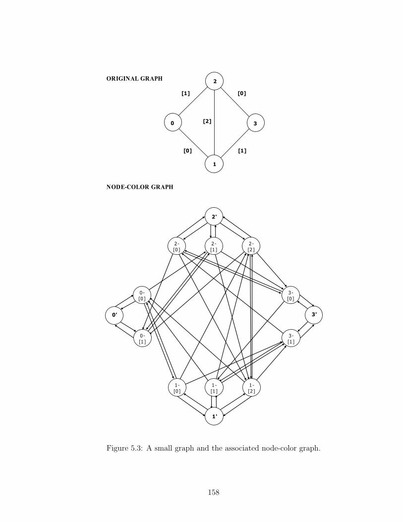
2'

1'

0' 3'

2-

[2]

2-

[0]

2-

[1]

3-

[1]

3-

[0]

1-

[2]

1-

[0]

1-

[1]

0-

[1]

0-

[0]

NODE-COLOR GRAPH

ORIGINAL GRAPH2

1

30

[1]

[0]

[0]

[1]

[2]

Figure 5.3: A small graph and the associated node-color graph.

158

Proposition 5.2 For an undirected colored graph GR = (VR, ER) the associated

directed node-color graph GC = (VC , AC) contains |VC | = |VR|+∑

i∈VRcdeg(i) nodes

and |AC | =∑

i∈VR2cdeg(i)+

∑{i,j}∈ER

(cdeg(i)+ cdeg(j)) arcs, where cdeg(i) is the

color degree of node i (i.e., the number of colors adjacent to the node).

Proof: Based on our construction technique the number of nodes in the node-color

graph is equal to the number of nodes in the original graph plus the number of

colors adjacent to each node. Therefore |VC | = |VR|+∑

i∈VRcdeg(i). There are two

types of arcs that we generate for the node-color graph. The first type is associated

with a node i′ representing the node i in the original graph and the nodes im, where

m ∈ C(i) representing the different colors adjacent to i. Since there are arcs from i′

to im and from im to i′ for all m ∈ C(i) we have∑

i∈VR2cdeg(i) such arcs. The second

type of arcs are “reload” arcs that are generated between the nodes of the node-color

graph that represent the different colors of each node. Observe, that a node i has

has cdeg(i) nodes associated with its colors. For each edge {i, j} in the original

graph we have to create cdeg(i) arcs from each of the cdeg(i) nodes of i to node jm

where m = C(i, j) (C(i, j) denotes the color of edge {i, j}) and cdeg(j) arcs from

each of the cdeg(j) nodes of j to node im where m = C(i, j). Therefore the number

of arcs of this type in the node-color graph is equal to∑

{i,j}∈ER(cdeg(i) + cdeg(j))

and |AC | =∑

i∈VR2cdeg(i) +

∑{i,j}∈ER

(cdeg(i) + cdeg(j)).

We use decision variables w{ij}, like before, to indicate whether edge {i, j} is

selected or not and we also define new decision variables zs,tin,jm

that indicate the

proportion of flow from s to t that uses arc (in, jm) of the node-color graph. Notice

159

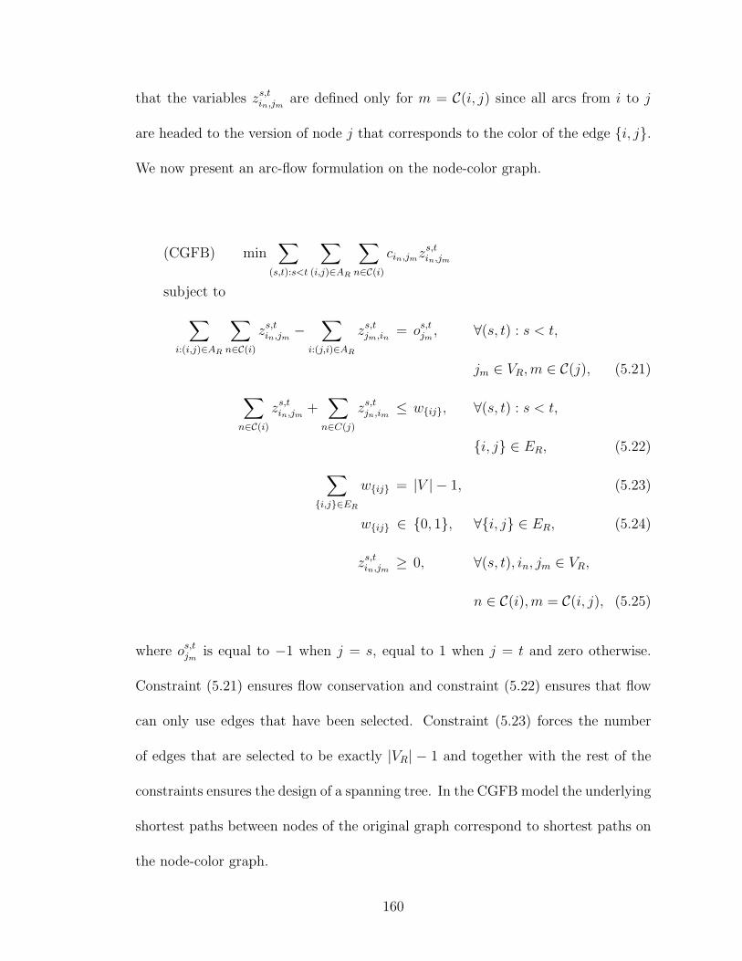
that the variables zs,tin,jm

are defined only for m = C(i, j) since all arcs from i to j

are headed to the version of node j that corresponds to the color of the edge {i, j}.

We now present an arc-flow formulation on the node-color graph.

(CGFB) min∑

(s,t):s<t

∑

(i,j)∈AR

∑

n∈C(i)cin,jmzs,t

in,jm

subject to

∑

i:(i,j)∈AR

∑

n∈C(i)zs,t

in,jm−

∑

i:(j,i)∈AR

zs,tjm,in

= os,tjm

, ∀(s, t) : s < t,

jm ∈ VR,m ∈ C(j), (5.21)

∑

n∈C(i)zs,t

in,jm+

∑

n∈C(j)

zs,tjn,im

≤ w{ij}, ∀(s, t) : s < t,

{i, j} ∈ ER, (5.22)

∑

{i,j}∈ER

w{ij} = |V | − 1, (5.23)

w{ij} ∈ {0, 1}, ∀{i, j} ∈ ER, (5.24)

zs,tin,jm

≥ 0, ∀(s, t), in, jm ∈ VR,

n ∈ C(i),m = C(i, j), (5.25)

where os,tjm

is equal to −1 when j = s, equal to 1 when j = t and zero otherwise.

Constraint (5.21) ensures flow conservation and constraint (5.22) ensures that flow

can only use edges that have been selected. Constraint (5.23) forces the number

of edges that are selected to be exactly |VR| − 1 and together with the rest of the

constraints ensures the design of a spanning tree. In the CGFB model the underlying

shortest paths between nodes of the original graph correspond to shortest paths on

the node-color graph.

160

Similarly to the LGFB formulation, the CGFB formulation can be strength-

ened using the following observation. Just like before when edge {i, j} is selected

then all commodities flowing to node a will flow either from i to j or from j to

i. Constraints (5.26) and (5.27) are equivalent to constraints (5.17) and (5.18) for

LGFB model in that they do not force all combinations of commodities and edges

and will have to be used with the existing set (5.22).

∑

n∈C(i)zi,a

in,jm+

∑

n∈C(j)zj,a

jn,im≤ w{ij}, ∀a ∈ VR, {i, j} ∈ ER, (5.26)

∑

n∈C(i)za,j

in,jm+

∑

n∈C(j)za,i

jn,im≤ w{ij}, ∀a ∈ VR, {i, j} ∈ ER. (5.27)

We also define constraints (5.28) and (5.29) which can replace constraint (5.22)

in the CGFB model and are equivalent to constraints (5.19) and (5.20) presented

earlier in the context of the LGFB model.

∑

n∈C(i)zs,a

in,jm+

∑

n∈C(j)zt,a

jn,im≤ w{ij},

∀(a, s, t) ∈ VR : {s < a, t < a}, {i, j} ∈ ER, (5.28)

∑

n∈C(i)za,s

in,jm+

∑

n∈C(j)za,t

jn,im≤ w{ij},

∀(a, s, t) ∈ VR : {a < s, a < t}, {i, j} ∈ ER. (5.29)

161

5.4 Reload Cost Problems - Extensions

Even though we have motivated reload costs through the VPN design in satel-

lite networks it is clear that they can appear under various contexts in the telecom-

munications and transportation industry. We now show how the two models devel-

oped in the Section 5.3 can be extended to deal with a variety of other problems in

which we face reload costs.

5.4.1 Routing Costs

In many problem contexts we incur a per unit of flow cost for routing com-

modities on the different edges in the network. In our original model, QFB, these

extra routing costs can be incorporated by augmenting the graph GR with copies i′

of each node i in VR and edges {i′, i} between the original nodes and the replicas.

The cost coefficient in the objective function can then be defined as cijk = Rnm+Ujk

where Rnm is the reload cost associated with going from edge {i, j} to edge {j, k}

(i.e., n = C(i, j) and m = C(j, k)) and Ujk is the per unit of flow routing cost on

edge {j, k}. As a result the routing costs can be considered as part of the reload cost

and do not have to be treated separately. In our later models, LGFB and CGFB,

these extra nodes, i′, already exist and can be used in the same fashion to allow for

routing costs.

162

5.4.2 Tree Network Design

In the previous section our objective was to minimize the total reload cost

incurred by the commodities. Wirth and Steffan in [83] define a reload cost problem

in which the objective is to build a minimum diameter spanning tree. In this case

we wish to minimize the maximum reload cost path on the tree network over all

commodities. Both the line graph and node-color models can be easily extended to

deal with this case. For both models we define a new decision variable g that will

be used to bound the total cost for the paths of all commodities. The line graph

model approach for the diameter minimization problem is presented below.

(D-LGFB) min g

subject to∑

(i,j,k)∈V ′R

cijkfs,tijk ≤ g, ∀(s, t) : s < t, (5.30)

g ∈ R+, (5.31)

(5.12), (5.13), (5.14), (5.15), (5.16).

The node-color model for the diameter minimization problem is similarly up-

dated.

(D-CGFB) min g

subject to∑

(i,j)∈AR

∑

n∈C(i)cin,jmzs,t

in,jm≤ g, ∀(s, t) : s < t, (5.32)

g ∈ R+, (5.33)

(5.21), (5.22), (5.23), (5.24), (5.25).

163

Naturally, we can augment both models with the sets of strengthening con-

straints introduced earlier. Specifically, for the line-graph model we can use con-

straints (5.17) and (5.18) in conjunction with (5.13) or replace (5.13) with (5.19) and

(5.20). Similarly, we can augment (5.22) in the node-color model with constraints

(5.26) and (5.27) or replace it with constraints (5.28) and (5.29).

The two models are also able to deal with non-unit demand problems between

origin and destination nodes. Such cases have been found to be harder that the unit

demand case discussed in Section 5.3. For such problems let ds,t be the demand

between s and t. The objective of the line graph model is then updated with the

following equation,

min∑

(s,t):s<t

∑

(i,j,k)∈V ′R

cijkds,tf s,t

ijk. (5.34)

The objective of the node-color model is updated similarly,

min∑

(s,t):s<t

∑

(i,j)∈AR

∑

n∈C(i)cin,jmds,tzs,t

in,jm. (5.35)

5.4.3 Uncapacitated Network Design

Another interesting problem that appears in the telecommunications and trans-

portation industries is the Uncapacitated Network Design (UND) problem. In this

problem there are costs associated with the routing of flow on the edges of the net-

work constructed but there are also fixed costs associated with the selection of the

edges. Quoting Balakrishnan et al. [8] the problem is “deceptively simple” and con-

164

tains other well-known problems as special cases, like the Steiner tree problem, the

uncapacitated facility location and the traveling salesman problem. In this section

we discuss Uncapacitated Network Design with reload costs.

Let Fij denote the installation cost of edge {i, j}. The line graph model for

the UND problem with reload costs can then be written as,

(U-LGFB) min∑

(s,t):s<t

∑

(i,j,k)∈V ′R

cijkfs,tijk +

∑

{i,j}∈ER

Fijw{ij}

subject to

(5.12), (5.13), (5.15), (5.16).

Observe that there is no constraint in this model that restricts the number of

edges to be selected. As a result the network designed is not restricted to the set

of spanning trees. We now present the node-color formulation that can be used for

the UND problem.

(U-CGFB) min∑

(s,t):s<t

∑

(i,j)∈AR

∑

n∈C(i)cin,jmzs,t

in,jm+

∑

{i,j}∈ER

Fijw{ij}

subject to

(5.21), (5.22), (5.24), (5.25).

Once again we note that there are no restrictions on the number of edges

that can be selected. Naturally, both of these models can be strengthened with the

same constraints we used to improve the original reload cost minimum spanning

tree problem as well as the diameter tree problem presented in this section.

165

Notice that with regular costs the UND problem is a general problem for

which the MST or OCST are special cases. The same is not true however, with the

version of the UND that incorporates reload costs. In other words, if we consider

the traditional UND with zero edge installation costs we get the OCST problem.

Additionally, when considering the UND with zero flow costs we get the MST prob-

lem. However, in the case of the UND with reload costs if we consider zero edge

installation costs the resulting solution will not necessarily be a tree.

5.5 Computational Results

In this section we will first explore the strengths of the reload cost tree prob-

lem formulations and evaluate the benefits of the additional forcing constraints we

presented earlier. We then compare the line graph model with the node color model.

Our computational work was conducted on a set of randomly generated prob-

lem instances with varying characteristics. All graphs were generated on a 100x100

grid. The endpoints for the edges were randomly picked among the nodes in the

graphs and the color for each edge was drawn from a uniform distribution. In the

tables that follow we identify each set as “NxEyCz” where x denotes the number

of nodes, y the number of edges and z the number of colors. Each set consists of 5

random problem instances. Unless otherwise noted all the reload costs between all

combinations of colors were set equal to 1. For our computational work we generated

problems where the number of nodes and edges in the graph varied between 5 and

20 and between 10 and 100, respectively. Also, we increase the number of different

166

colors in a graph from 3 to 9. The formulations were solved with CPLEX 9.0 on

a Windows PC with two Pentium Xeon processors at 2.66 GHz with 2 GBytes of

RAM.

5.5.1 Forcing Constraints

We first compare the percentage gaps between the LP relaxation of the various

versions of the CGFB model with optimal solutions. We will refer to the set of forcing

constraints (5.22) with which the CGFB model was presented initially as “set 1”.

Also, we refer to constraints (5.26) and (5.27) in addition to constraint (5.22) as

“set 2”. Additionally, “set 3” denotes the use of constraints (5.28) and (5.29).

Table 5.1 presents the average primal bound of the LP relaxation of the CGFB

model with the forcing constraints of set 1 for various problem sets. The table also

presents the average percentage IP-LP gap calculated as the difference between the

values of the LP bound and the optimal integer solution, over the value of the

LP bound. The last column in the table shows the average running time of the LP

relaxation in seconds. In a similar fashion, Table 5.2 presents the solutions of the LP

relaxation of the CGFB model with the use of the forcing constraints of set 2. Just

like before the table presents the average primal solution, the average percentage

IP-LP gap and the average running time for the relaxation. The last column in

this table provides the average percentage improvement of the LP bound from the

CGFB model with constraint set 1. This improvement is calculated as the difference

between the LP bound with set 1 and set 2 over the value of the LP bound with

167

set 1. Table 5.3 has exactly the same structure as Table 5.2 and provides solution

information for the CGFB model with constraint set 3. The only difference is that

the average percentage improvement presented is over the the set 2 solutions.

From the information presented in these tables it is clear that the forcing

constraints associated with sets and 2 and 3 can provide improvements over the

original model. However, notice that these improvements come with a penalty in

terms of the computation time required. These computational penalties are a direct

consequence of the increased number of constraints in the various formulations. For

example consider a problem with 15 nodes and 50 edges (the number of colors does

not affect the number of forcing constraints). For this problem, the number of forcing

constraints in Set 1 is equal to the number of half-pairs of commodities times the

number of edges. The number of half-pairs is equal to the combination of 15 over 2

which is 105. So the number of set 1 forcing constraints is 105 · 50 = 5, 250. For set

2 we add the extra constraints which are equal to 2 ·15 ·50 = 3, 000 and reach a total

of 3, 000 + 5, 250 = 8, 250 constraints. For set 3 we consider triplets of nodes, which

are given by∑|V |

n=1 n2. Therefore for 15 nodes we have 1, 240 triples. As a result

the number of constraints is 2 · 1, 240 · 50 = 124, 000. From this example it should

be clear that the significant increase in the size of the formulation is causing the

very large computation times observed. Based on the improvement percentages and

computation times presented in Table 5.3 for problems with 15 nodes one can argue

that the extra running time associated with set 3 outweighs the benefits introduced.

Based on this observation we have not tested the constraints associated with set 3

on problems with more than 15 nodes. Also, notice that for graphs with a specific

168

Problem Set Primal IP-LP Gap (%) Time (s)

N5E10C3 0.00 0.00 0.025

N10E25C3 3.70 44.00 0.137

N10E25C5 9.65 10.79 0.137

N10E25C7 23.67 8.72 0.206

N15E50C3 3.48 128.70 4.125

N15E50C5 28.50 14.32 2.038

N15E50C7 49.96 17.04 3.419

N15E50C9 71.17 11.80 4.231

N20E100C3 0.00 0.00 132.519

N20E100C5 4.94 417.41 115.187

N20E100C7 26.48 61.58 48.125

N20E100C9 58.40 23.19 43.897

Aggregate 16.26 54.40 21.84

Table 5.1: LP relaxation results for the CGFB model with the forcing constraints

of set 1.

number of nodes and edges, increasing the number of different colors seems to make

the problems easier. This is particularly clear in Table 5.2. Even though at first this

might seem counterintuitive observe that in the extreme case in which the number

of different colors equals the number of edges in a graph all trees are associated with

the same total reload cost and therefore all trees are optimal. Of course the other

extreme, in which all edges have the same color also presents a trivial case, where

any tree would again be an optimal solution.

5.5.2 Comparison of LGFB vs. CGFB

We now focus our attention on the differences between the line graph and node

color models. Table 5.4 presents the average percentage gaps between the optimal

169

Problem Set Primal IP-LP Gap (%) Time (s) Improvement (%)

N5E10C3 0.00 0.00 0.031 0.00

N10E25C3 5.24 44.00 0.206 28.82

N10E25C5 10.93 10.79 0.209 9.19

N10E25C7 24.64 8.72 0.287 4.16

N15E50C3 6.69 128.70 11.209 66.70

N15E50C5 31.62 14.32 4.181 9.37

N15E50C7 53.92 17.04 7.353 9.33

N15E50C9 74.62 11.80 9.516 4.81

N20E100C3 0.00 0.00 474.784 0.00

N20E100C5 13.42 417.41 404.428 239.01

N20E100C7 36.51 61.58 208.913 47.94

N20E100C9 65.43 23.19 149.390 11.63

Aggregate 18.42 8.54 76.02 30.95

Table 5.2: LP relaxation results for the CGFB model with the forcing constraints of

set 2. The “improvement” column represents average percentage improvement over

the set 1 constraints.

Problem Set Primal IP-LP Gap (%) Time (s) Improvement (%)

N5E10C3 0.00 0.00 0.028 0.00

N10E25C3 5.42 5.20 2.800 1.77

N10E25C5 11.20 0.00 1.009 1.39

N10E25C7 25.25 1.91 2.097 2.20

N15E50C3 8.01 15.16 3782.663 11.77

N15E50C5 32.33 2.85 2812.165 1.47

N15E50C7 56.06 2.80 4655.703 4.14

N15E50C9 76.87 3.47 2437.356 3.00

Aggregate 17.93 3.23 1,141.15 2.77

Table 5.3: LP relaxation results for the CGFB model with the forcing constraints of

set 3. The “improvement” column represents average percentage improvement over

the set 2 constraints.

170

solutions and the LP relaxation of both the line-graph and node-color graph models

for all three sets of forcing constraints. From the table we see that even thought

the two approaches are distinctly different the two models have the same strength

under all the different types of forcing constraints.

Table 5.5 presents the average running times of the LP relaxations of both

models under the different sets of forcing constraints. From the information in the

table it is easy to declare the model associated with the node-color graph as the

clear winner since its average running times are always lower than the ones for the

line graph model. This difference in running times can be partially explained by

the differences in the dimensions of the associated graphs, in terms of number of

nodes and number of edges involved. Table 5.6 shows the average number of nodes

and edges for the two graphs for the different problems solved. For the selected

problems the line graph includes always a larger number of nodes and in most cases

a larger number of edges. As expected, the node color graph depends heavily on the

number of different colors in a problem. We could potentially generate problems

that have an even higher number of different colors and in which the color graph

will have a larger number of nodes and edges over the line graph. However, based

on our earlier observations concerning the number of different colors in a graph we

expect the node color graph to still fair better.

171

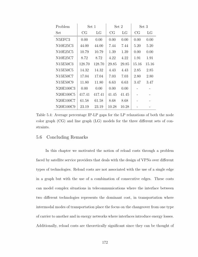
Problem Set 1 Set 2 Set 3

Set CG LG CG LG CG LG

N5EFC3 0.00 0.00 0.00 0.00 0.00 0.00

N10E25C3 44.00 44.00 7.44 7.44 5.20 5.20

N10E25C5 10.79 10.79 1.39 1.39 0.00 0.00

N10E25C7 8.72 8.72 4.22 4.22 1.91 1.91

N15E50C3 128.70 128.70 29.85 29.85 15.16 15.16

N15E50C5 14.32 14.32 4.43 4.43 2.85 2.85

N15E50C7 17.04 17.04 7.03 7.03 2.80 2.80

N15E50C9 11.80 11.80 6.63 6.63 3.47 3.47

N20E100C3 0.00 0.00 0.00 0.00 - -

N20E100C5 417.41 417.41 41.45 41.45 - -

N20E100C7 61.58 61.58 8.68 8.68 - -

N20E100C9 23.19 23.19 10.28 10.28 - -

Table 5.4: Average percentage IP-LP gaps for the LP relaxations of both the node

color graph (CG) and line graph (LG) models for the three different sets of con-

straints.

5.6 Concluding Remarks

In this chapter we motivated the notion of reload costs through a problem

faced by satellite service providers that deals with the design of VPNs over different

types of technologies. Reload costs are not associated with the use of a single edge

in a graph but with the use of a combination of consecutive edges. These costs

can model complex situations in telecommunications where the interface between

two different technologies represents the dominant cost, in transportation where

intermodal modes of transportation place the focus on the changeover from one type

of carrier to another and in energy networks where interfaces introduce energy losses.

Additionally, reload costs are theoretically significant since they can be thought of

172

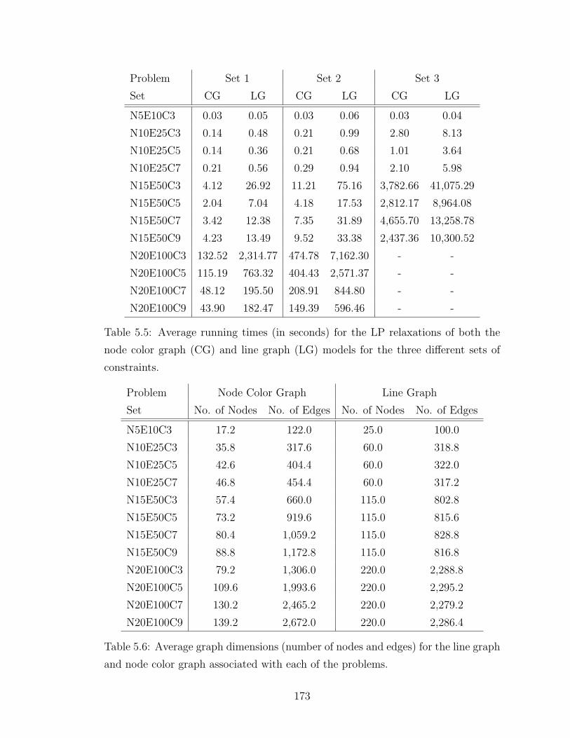
Problem Set 1 Set 2 Set 3

Set CG LG CG LG CG LG

N5E10C3 0.03 0.05 0.03 0.06 0.03 0.04

N10E25C3 0.14 0.48 0.21 0.99 2.80 8.13

N10E25C5 0.14 0.36 0.21 0.68 1.01 3.64

N10E25C7 0.21 0.56 0.29 0.94 2.10 5.98

N15E50C3 4.12 26.92 11.21 75.16 3,782.66 41,075.29

N15E50C5 2.04 7.04 4.18 17.53 2,812.17 8,964.08

N15E50C7 3.42 12.38 7.35 31.89 4,655.70 13,258.78

N15E50C9 4.23 13.49 9.52 33.38 2,437.36 10,300.52

N20E100C3 132.52 2,314.77 474.78 7,162.30 - -

N20E100C5 115.19 763.32 404.43 2,571.37 - -

N20E100C7 48.12 195.50 208.91 844.80 - -

N20E100C9 43.90 182.47 149.39 596.46 - -

Table 5.5: Average running times (in seconds) for the LP relaxations of both the

node color graph (CG) and line graph (LG) models for the three different sets of

constraints.

Problem Node Color Graph Line Graph

Set No. of Nodes No. of Edges No. of Nodes No. of Edges

N5E10C3 17.2 122.0 25.0 100.0

N10E25C3 35.8 317.6 60.0 318.8

N10E25C5 42.6 404.4 60.0 322.0

N10E25C7 46.8 454.4 60.0 317.2

N15E50C3 57.4 660.0 115.0 802.8

N15E50C5 73.2 919.6 115.0 815.6

N15E50C7 80.4 1,059.2 115.0 828.8

N15E50C9 88.8 1,172.8 115.0 816.8

N20E100C3 79.2 1,306.0 220.0 2,288.8

N20E100C5 109.6 1,993.6 220.0 2,295.2

N20E100C7 130.2 2,465.2 220.0 2,279.2

N20E100C9 139.2 2,672.0 220.0 2,286.4

Table 5.6: Average graph dimensions (number of nodes and edges) for the line graph

and node color graph associated with each of the problems.

173

as an extension to the Optimum Communications Spanning Tree (OCST) problem

in the same way that the Quadratic Spanning Tree (QST) problem is an extension to

the MST. Despite their wide application context and theoretical importance reload

costs have only recently been treated in the literature in a paper by Wirth and

Steffan [83]. In this chapter we look at different problems with reload costs and

formulate several models that can solve them exactly.

We primarily look at the problem of finding a spanning tree that minimizes

the total reload costs associated with sending flow between all pairs of nodes in

a graph. We first present a mathematical formulation with a quadratic objective

function and then linearize this objective with a transformation that leads us to

the notion of a line graph. We then approach the problem from a significantly

different viewpoint and develop a model that is based on what we call a node color

graph. Both models are strengthened with the use of extra forcing constraints that

were originally developed in the context of uncapacitated network design (see [8]).

We then proceed to discuss several other classic network design problems where

traditional costs are replaced by reload costs and showcase the applicability of our

approaches in all these cases.

Our computational work focuses on the strength of the LP relaxation of the

reload cost tree problem that motivated this work. Our strongest model results in

an LP relaxation that is on average only 3.23% from optimality. However, this gap

requires on average more than a 1, 000 seconds of running time to be achieved. We

also provide a slightly weaker model with fewer constraints that can achieve a more

modest 8.54% within 76 seconds on average. We then compare the line graph model

174

with the node-color model and find that the node-color graph is consistently faster.

Both of the extended graphs that we developed in this chapter allow us to

assign reload costs to specific edges rather than pairs of edges. Moreover, each path

in the original graph is associated with a specific path on both the line-graph and

node-color graph. As a result it is natural to think that a path-based model for

reload cost problems in which the pricing problem is solved on one of these two

graphs might result in a faster solution procedure. In the appendix we present the

theoretical groundwork for such a formulation and the associated branch-and-price

approach.

175

Chapter 6

Summary, Contributions, and Concluding Remarks

6.1 Summary

This dissertation was largely motivated by the various challenges that man-

agers and network planners for satellite service providers face in practice. Ever

since their inception in 1945 satellite services have captured the imagination of the

public and provided the technical capabilities as well as the business potential for

unique, worldwide communication services. The satellite industry has experienced

significant growth in its short 50-year-old history and has currently grown to a 60

billion dollar sector of the telecommunication services industry. Moreover, satellites

have connected the world community unlike any other communications medium

by allowing the live broadcasting of worldwide sporting events and breaking news.

Despite the satellite services industry’s tremendous communications potential, its

current size and growth opportunities and the significant challenges associated with

its successful operation it has not attracted a lot of attention from the academic

management science community in recent years. The main focus of this dissertation

was on the core operational concerns of modern day satellite service providers that

operate a fleet of geosynchronous satellites and offer diverse services to thousands

of customers all around the world. The critical challenge that we had to face and

is at the core of all the problems we treat here has to do with determining how

176

to route the services for all the different customers of a provider over its satellite

and terrestrial network. While routing this traffic we have to take into account not

only the technical restrictions that are inherent to satellite communications but also

the prevailing business practices that sometimes impose constraints and financial

penalties on our decisions.

In Chapter 2 we discussed the problem of routing traffic in a satellite network

and highlighted the significant differences of this problem when compared to tradi-

tional traffic routing problems over terrestrial communications and other networks.

Specifically, we point out that routing in a satellite network is not transparent to the

end user and typical service level agreements impose significant financial penalties to

satellite service providers when they force a customer on a different route than what

was originally agreed upon. This distinctive characteristic of the business model

currently used in the satellite services sector can have a dramatic effect on planning

decisions and the costs associated with a specific routing plan. In the model we

propose in Chapter 2 we take into account these rerouting penalties and look at

the traffic routing problem of satellite service providers over an extended time hori-

zon. The time dimension allows us to capture the effects of possible reroutings and

make the best traffic routing decisions that will ultimately allow the satellite service

provider to satisfy as much customer demand as possible while minimizing its costs.

Also, the extended time horizon encompasses changes in the very dynamic topology

of satellite networks as well as potential trends in the demand patterns they try to

satisfy. In our technical discussion of the mathematical model we develop to ap-

proach this problem we first observe that the traditional multicommodity arc-flow

177

formulations that have been used in the past for similar problems require an inor-

dinate number of decision variables to capture the rerouting penalties. Instead we

develop a novel approach that is based on the idea of super-paths that describe the

routing decisions for a customer over the entire planning horizon rather than just a

single period. The resulting integer program has an exponential number of columns

but a smaller (compared to a potential arc-flow model) number of constraints. These

types of models are successfully solved with a column generation procedure in which

we only consider a reduced version of the formulation that only includes a limited

number of columns. A pricing problem is then solved that determines whether addi-

tional columns are needed or the optimal linear relaxation solution has been reached.

In our problem the columns of the mathematical formulation describe super-paths

as opposed to traditional paths. As a result the associated pricing problem presents

novel challenges that cannot be treated with known methodologies. The complicat-

ing factor is associated with the fact that the cost of a super-path does not only

consist of the traditional routing costs over the planning horizon’s time periods but

also includes the possible rerouting penalties. We therefore develop an approach

that constructs a specialized pricing graph that can deal with the pricing problem

associated with the super-paths. We then present a branch-and-price-and-cut ap-

proach that uses this pricing graph to add columns at the different nodes of the

search tree and also uses straightforward lifted cover inequalities to improve upon

the LP relaxation bounds. Our computational analysis in this chapter presents em-

pirical evidence on the strengths of using the branch-and-price-and-cut procedure

that considers the entire planning horizon as opposed to a simple period-by-period

178

approach that looks at each period individually and makes specific traffic routing

decisions for that period before moving on to the next. Our results show that the

BPC procedure is approximately 8% to 11% better than the period-by-period ap-

proach for nominal problem parameters but can provide improvements up to 25%

for higher values of the rerouting penalty. We also test our approach for problems

with varying number of time periods and customers and find that the improvement

percentages remain fairly constant whereas the computational effort is not adversely

affected by the increased time periods and seems to increase only for larger numbers

of customers. Additionally, we test a “root-node” procedure that generates new

columns only at the root node of the search tree and compare it to the branch-and-

price-and-cut approach. This altered approach can in some cases provide results

that are comparable to the full blown procedure. Finally, we present a real life case

in which the root-node procedure was used for the planning of a satellite network

with 30 satellites and 1, 500 customers and provided a solution that improved upon

the existing period-by-period approach by 40% or $200 million dollars. We believe

that our work on the deterministic multiperiod traffic routing problem addresses

key issues in satellite network planning and allows managers to make decisions that

significantly reduce operational costs when compared to existing approaches. The

proposed branch-and-price-and-cut procedure is a tractable, exact approach that

solves a challenging problem. The two novel ideas behind this procedure are the re-

formulation based on super-paths and the construction of the pricing graph. These

ideas are extended to encompass general types of rerouting penalties in the context

of multicommodity flows and can therefore potentially provide improvements upon

179

existing procedures in other applications in which reconfigurations (or reroutings)

are penalized. More importantly the MPTR problem is a natural extension to the

IMCF problem, the importance of which cannot be overstated. As such the MPTR

model, extends multicommodity flow applications and methodology over multiple

stages (time periods) and can therefore capture much more general problems than

traditional IMCF models.

In Chapter 3 we look at an extension of the traffic routing problem in which

we consider network design decisions in addition to the traffic routing decisions

we focused on the previous chapter. In the context of satellite service providers

network design has to do with the onboard configuration of the various satellites.

Network planners have the capability to change the onboard configuration of a

geosynchronous satellite in order to allow for better coverage of specific regions of

the world, to enhance existing services or to implement new services. It is important

therefore for managers in the satellite service industry to be able to decide on the

best configuration to be used for each satellite. The main tradeoff they face is that

changing the configuration of a satellite to better service an emerging market the

provider would undoubtedly have to reroute several service requests and incur a

number of penalties. As a result it is important to make the configuration decisions

while also considering the traffic routing of the all the different service requests. We

approach this problem with a mathematical model that uses the idea of super-paths,

developed earlier, and is also complemented by design variables that indicate how

the different satellites should be configured. The resulting solutions from this model

provide the necessary configurations that will allow the satellite service provider to

180

satisfy as much of the demand as possible while minimizing its operational costs.

Once again the main challenge in solving this problem with a branch-and-price-and-

cut approach is the pricing problem that will determine the columns that have a

negative reduced cost. We show how the approach we developed in the previous

chapter can be extended to deal with this pricing problem, but more importantly

we discuss extensions to a much more general class of penalty costs. Specifically, we

point out how these cost structures might appear in other multiperiod traffic routing

and network design problems in which rerouting penalties are more elaborate and

not only depend on the time period in which the rerouting occurs but are also a

function of the paths before and after the rerouting. We evaluate the strength of

our branch-and-price-and-cut procedure by comparing it to the period-by-period

and the root-node approaches we presented in the previous chapter. The results

indicate that as the number of configurations which the planners have to take into

account increases the benefits of using a BPC solution procedure increase to 12%

when compared to the period-by-period approach and to 30% when compared to the

root-node procedure. Our computational analysis shows that unlike our observations

in the earlier chapter when network design variables are involved in our problem the

root-node procedure is significantly outperformed, even by a short-sighted period-

by-period approach. Moreover, we observe that even though it is possible to define

the network design variables that specify which configuration to use as linear it is

actually computationally faster to define them as binary. This is because branching

on the binary design variables first can significantly reduce the number of super-

paths that we have to consider. The results presented in this chapter in the context

181

of satellite networks can easily be extended to deal with multistage capacitated

network design in general. What is important to point out here is that the super-

path reformulation and the associated BPC procedure can seamlessly be extended

for an arbitrary number of time periods without significant computational penalties.

Also, even though in this chapter we treat a general rerouting penalty structure the

MPCAP problem and our BPC procedure is relevant even when there are no such

penalties.

In Chapter 4 we relax one of the central assumptions we made for the two

previous chapters, namely that future demand information is known with certainty

and we can therefore plan for an extended planning horizon with the help of a de-

terministic model. We point out that large satellite service providers have long-time

customers that sometimes sign contracts for multiple years and in that sense plan-

ners feel confident in their forecasts for future customer demands. This is what

makes the solutions from the models of the two previous chapters worthy for net-

work planners to consider in their decision making process. However, even though

forecasts for individual demands might be trustworthy, by taking into account un-

certainty in the market conditions that affect these demands it is possible to plan

for many contingencies and therefore have a solution that will stand up to chang-

ing market conditions. In order to account for the random nature of the prevailing

trends in the marketplace we allow for network planners to define discrete stochas-

tic scenarios, their probability of occurring and their effect on all the existing and

future customers considered in the planning horizon. We model this problem as a

multistage stochastic multicommodity flow problem with integer recourse. In our

182

overview of related papers in the literature we point to the lack of exact solution

procedures that can deal with multistage stochastic problems with integer recourse.

The arc-flow formulation we present at first specifies auxiliary variables that are used

to capture the rerouting penalties from one time period to the next and nonantic-

ipativity constraints to guarantee that decisions in each time period rely only on

the information known up to that point in time. However, this model can only be

used with the typical L-Shaped method which we showcase for the linear relaxation

of a two-stage problem. We then point to the significant complications involved

in extending this method to deal with integer variables and multiple stages. We

continue by presenting a reformulation that is based on the idea of introducing one

variable that will represent all decisions made for each scenario and across all time

periods. The resulting model is similar to the path-based formulation we presented

in Chapter 2 but it involves one super-path variable for each scenario considered

and a set of nonanticipativity constraints. In solving this problem we use a branch-

and-price-and-cut approach similar to the one developed earlier. We then go on and

treat a general multistage network design problem with demand uncertainty and

develop an exact solution procedure that can be used even when decision variables

at all stages are integer and regardless of the number of stages. This approach is

based on the reformulation idea and the BPC procedure we presented earlier. In

addition, we discuss the robust counterpart to the stochastic model we developed

and under which contexts a robust rather than a stochastic solution would be prefer-

able. In our computational experiments we present evidence of the benefits that can

be realized by using a stochastic over a deterministic approach by comparing the

183

stochastic solutions with solutions we get from our deterministic BPC procedure

by using expected demand information. Specifically, the stochastic solutions are on

average between 4.8% and 11.7% better that the solutions based on expected values.

In absolute terms we found the value of the stochastic solution to be worth between

$4.1 and $8.8 million to a small satellite service provider with a network of only two

satellites. We also compared the stochastic solutions to what would have been pos-

sible if perfect information was available to the planners. Our results indicate that

the problems become harder as the aggregate demand that needs to be routed or the

number of scenarios we consider increase. The average gap between the stochastic

solutions and the wait-and-see solutions are for most problem sets less than 5%,

on average. More importantly, we believe that our computational analysis shows

that we can efficiently approach multistage stochastic problems with 5 stages and

integer variables for all stages even when we consider 40 random scenarios. Even

though our work on the multistage stochastic multicommodity flow problem was

presented as an extension to the deterministic problem developed earlier we believe

that it represents a step forward in the treatment of integer stochastic programs

in general. In particular for multicommodity flow network design problems with

uncertain demand our approach provides a computationally efficient, exact solution

procedure.

In Chapter 5 we consider a problem that is motivated by the planning and

offering of a particular service to customers of satellite networks. Specifically, large

organizations require Virtual Private Networks (VPN) to interconnect their geo-

graphically dispersed locations and satisfy all their data, voice, and video commu-

184

nication needs. These VPNs typically consist of communication links that utilize

different technologies like satellite, fiber and copper. The dominant costs that we

need to take into account when designing a VPN are related to the equipment re-

quired to interface the different technologies rather than the per unit of traffic cost

associated with utilizing any of the communication links. These special costs are

referred to as reload costs and have significant applications in the telecommunica-

tions and transportation industries. Despite the fact that they can model complex

cost structures in such important areas they have only been treated recently, and

very briefly, in the literature. In our analysis we first present a straightforward arc-

flow model that has a quadratic objective function. We proceed to develop another

arc-flow model with a linear objective that refers to flow variables on a significantly

more complex graph. This graph is a directed line-graph in which reload costs are

associated with single arcs rather than combinations of them. Moreover, all paths

in the line-graph have a one-to-one correspondence with the paths in the original

graph. We then improve upon this model by using traditional strengthening tech-

niques that introduce additional forcing constraints between the flow variables and

network design variables. Our theoretical treatment of reload costs continues with

the development of a second model that once again introduces an expanded graph

that associates the reload costs with specific arcs. We call this graph the node-color

graph and its size, unlike the earlier line-graph, depends on the number of different

colors in the original graph. We strengthen the arc-flow model that is based on this

graph with the same techniques we used to improve the line-graph model. Before

presenting computational results on the strengths of these two models we look at

185

several typical extensions to the traditional minimum spanning tree design prob-

lem we treated. Specifically, we consider the non-unit demand case as well as the

minimum diameter spanning tree and the uncapacitated network design problem

with reload costs and provide the appropriate extensions to our two models that

can treat these cases. In our computational work we first examine the effects of the

two extra sets of forcing constraints that we use with the line-graph and node-color

models. Our results show that the first set of additional constraints improves the LP

relaxation of the original model by approximately 31% and runs on average within

80 seconds. The second set of additional forcing constraints further improves the

LP relaxation. On average, the extra constraints improve the bound we get from

the first set by 2.77% but require a running time of more than 1, 000 seconds, on

average. We conclude the chapter by remarking that the line-graph and node-color

models naturally lend themselves to path-based approaches. A path-based model

would have a significantly simpler formulation because reload costs would be just a

part of the path costs. However, in these models we would require the line and node-

color graphs to solve the associated pricing problems. We present the theoretical

groundwork for such a formulation and the required branch-and-price procedure in

the appendix. We strongly believe that reload costs are able to capture important,

complex cost structures that have already been identified in applications in telecom-

munications and transportation. Our presentation of different models that are able

to simplify these costs and transform them to simple variable edge costs allows the

use of standard solution approaches and strengthening techniques already available.

186

6.2 Further Research and Application Opportunities

Applications in the satellite context can be further enhanced to include deci-

sions on relocation, launches and discontinuation of service of the different satellites

in the spacecraft fleet of a large satellite service provider. Also, aspects of the terres-

trial network of such large providers, such as antenna (satellite dishes) and optic link

capacities, can be integrated in the planning. Specifically, antennas owned by large

providers are a critical part of the provider’s infrastructure and are associated with

various complicating factors including visibility issues, signal strength limitations,

etc.

Rerouting or reconfiguration penalties can appear in settings other than satel-

lite networks. Specifically, in production planning for multiple stages (time periods)

the setup and changeover costs from one type of production to another (for the pro-

duction of different products) can be a significant cost factor. Additionally, in the

context of terrestrial telecommunication networks and optical networks in particu-

lar when planning for contingency scenarios in case of network failures we typically

wish to minimize the number of different paths to be used over all contingencies.

The differences in paths can be potentially modeled as rerouting penalties and the

various contingencies can be treated as multiple stages in our procedure context.

For integer stochastic programs in general it is possible that a similar reformu-

lation to the one presented in this dissertation and an appropriate decomposition

of the primal problem might significantly help solve problems with more than two

stages efficiently. The main challenge would be to appropriately define a compact

187

model and find efficient ways to solve the associated pricing problem.

In the context of satellite network planning failures on satellites have very sig-

nificant implications to the operation of the network since there is no way to recover

the spacecraft and restore (in the short term) the lost capacity. A practical exten-

sion to our stochastic problem would include scenarios for infrastructure failures and

would therefore involve uncertainty in the right-hand-side of the constraints of the

formulations presented. From a practical standpoint this would be a very important

step for planners in the satellite industry.

Reload costs constitute both a significant theoretical construct as well as an

important practical tool. It is therefore important to look into specialized exact and

approximation algorithms that can deal with these costs directly and achieve im-

provements on the results presented here in terms of the LP relaxation strength and

computational efficiency. The most direct approaches could come from construc-

tion heuristics, local search approaches and genetic algorithms. However, stronger

formulations utilizing more efficient extended graphs could also be possible.

Finally, we would like to point out that even though column-generation has

been around for several decades it has only gained popularity recently. However,

general frameworks for the implementation of branch-and-price approaches are very

few and are typically characterized by very steep learning curves. Additionally,

apart from implementation issues researchers at the forefront of column-generation

are constantly experimenting with new branching and cutting strategies, and more

importantly new compact formulations and their associated pricing problems. Our

experience with the BPC approaches presented here have shown that these proce-

188

dures hardly ever work straight out of the box. In other words a straightforward

branch-and-price procedure will hardly ever provide exceptional results. In order to

get improvements over other existing methodologies one has to look at adding cuts,

improving the branching implementation and also incorporating heuristics in the

search. Therefore, research on branch-and-price approaches presents opportunities

in many areas of integer programming.

189

Appendix - Column Generation for Reload Costs

In Section 5.3 we presented two approaches that associate shortest paths on

a simple graph with a complex cost structure (i.e., quadratic) with shortest paths

on more complicated graphs but with a straightforward (i.e., linear) cost structure.

Both approaches naturally lend themselves to the solution of path based (instead

of arc-flow) formulations. We now look at the original minimum cost spanning tree

problem with reload costs and formulate it with the use of paths.

Let xs,tp be one if path p is used by commodity (s, t) and zero otherwise. Also,

let P s,t be the set of paths from s to t. We now present a path-based formulation

for the minimum cost spanning tree with reload costs on the original graph GR.

(RCPATH) min∑

(s,t):s<t

∑

p∈P s,t

cs,tp xs,t

p

subject to

∑

p∈P s,t

xs,tp δp

ij +∑

p∈P s,t

xs,tp δp

ji ≤ w{ij}, ∀(s, t) : s < t, {i, j} ∈ ER, (6.1)

∑

p∈P s,t

xs,tp = 1, ∀(s, t) : s < t, (6.2)

∑

{i,j}∈ER

w{ij} = |VR| − 1, (6.3)

xs,tp ≥ {0, 1}, ∀(s, t) : s < t, p ∈ P s,t, (6.4)

w{ij} ∈ {0, 1}, ∀{i, j} ∈ ER. (6.5)

where δpij is a coefficient that is one if arc (i, j) is used by path p and zero otherwise.

cs,tp is the cost of path p from s to t and will contain all reload costs associated with

that path. Constraint (6.1) states that when edge {i, j} is selected then the paths

190

will have to either traverse that edge from i to j or in the other direction. Constraint

(6.2) forces the selection of exactly one path for each commodity and constraint (6.3)

restricts the number of edges to be selected. Since paths are constructed between

all half-pairs of nodes in VR and exactly one path has to be selected, constraint (6.3)

will force the design to be a spanning tree. Constraints (6.4) and (6.5) define the

edge variables as non-negative and the edge variables as binary, respectively.

As with the arc-flow models we will now introduce two extra pairs of con-

straints that can be used to strengthen the initial RCPATH model. These con-

straints are based on the same observations that we made previously and their only

difference is that they deal with path variables instead of flow variables. Constraints

(6.6) and (6.7) make sure that when edge {i, j} is selected paths use this edge either

in the direction from i to j or vice versa. However, as we have noted previously

(see Section 5.3.2 or 5.3.3) these constraints do not include all commodity and edge

combinations and have to be used in addition to constraint (6.1).

∑

p∈P i,a

xs,ap δp

ij +∑

p∈P t,a

xj,ap δp

ji ≤ w{ij}, ∀a ∈ VR, {i, j} ∈ ER, (6.6)

∑

p∈P a,j

xa,sp δp

ij +∑

p∈P a,t

xa,ip δp

ji ≤ w{ij}, ∀a ∈ VR, {i, j} ∈ ER, (6.7)

We also present constraints (6.8) and (6.9) that can replace constraint (6.1)

since they force each edge {i, j} to be used in one direction only, for all edge and

commodity combinations.

191

∑p∈P s,a

xs,ap δp

ij +∑

p∈P t,a

xt,ap δp

ji ≤ w{ij}, ∀(s, t, a) ∈ VR : {s < a, t < a}, {i, j} ∈ ER,

(6.8)

∑p∈P a,s

xa,sp δp

ij +∑

p∈P a,t

xa,tp δp

ji ≤ w{ij}, ∀(s, t, a) ∈ VR : {a < s, a < t}, {i, j} ∈ ER,

(6.9)

The RCPATH model defines the design variables as binary and the path vari-

ables as linear in the same way the arc-flow models did. However, observe that it is

possible to define the path variables as binary and relax the edge selection variables

and still get integer feasible solutions. Let w{ij} ∈ R+ for all {i, j} and xs,tp ∈ {0, 1}

for all (s, t) and p ∈ P s,t. Let A be a matrix consisting of the w{ij} coefficients from

constraints (6.1) and (6.3). Specifically, matrix A has the following form,

−w{ij} ≤ −∑

p∈P s,t

xs,tp δp

ij −∑

p∈P s,t

xs,tp δp

ji

∑

{i,j}∈ER

w{ij} = |VR| − 1

Each row in A, except the last, contains a single −1. In proving that this is a totaly

unimodular (TU) matrix we can delete these rows and end up with the last row

that is entirely made up with ones. Therefore we can delete all columns in this last

row and end up with an empty matrix that is TU. Based on Proposition 2.1 from

Nemhauser and Wolsey (see p. 540 in [63]) A will also be TU. Proposition 2.2 in

Nemhauser and Wolsey (see p. 541 in [63]) states that a polyhedron P = {x ∈

192

R+ : Ax ≤ b} is integral for all b ∈ Z. In our case the last row of b is equal to

|VR| − 1 and the rest of the rows are equal to 0 or −1 because of constraint (6.2).

Therefore b is integral and polyhedron P will have integer extreme points. As a

result relaxing the binary constraints on the edge selection variables w{ij} will give

the same solution as the original RCPATH model.

Pricing

In our exposition of the pricing problem for the RCPATH model we treat the

most general case in which the formulation contains constraints (6.8) and (6.9).

Similar conclusions can be drawn for all other cases. The reduced cost of a path p

for commodity (n,m) in the RCPATH model is given by the following equation,

cn,mp = cn,m

p +∑

{i,j}∈ER

∑q∈VR

(πnqm

ij δpij + πqnm

ij δpji + πmqn

ij δpij + πqmn

ij δpji

)− σn,m (6.10)

where −πstaij is the dual of constraint (6.8), −πsta

ij is the dual of constraint (6.9) and

σs,t is the dual of constraint (6.2). Notice that the dual values −πstaij and −πsta

ij are

defined only for {s < a, t < a} and {a < s, a < t}, respectively. In all other cases

we set −πstaij and −πsta

ij equal to zero.

The cost of a path can be written as cp =∑

(i,j,k) cijkδpijk, where δp

ijk is one if

arc (j, k) is used immediately after arc (i, j) on path p. We have used the notation

cijk before in Section 5.3 to refer to the reload costs associated with using arc (j, k)

immediately after arc (i, j). However, this decomposition is not very helpful since in

equation (6.10) we have the coefficients δpij that depend on specific arcs (i, j) instead

193

of triplets (i, j, k). Therefore the pricing problem associated with the columns of

the RCPATH model is not a straight forward shortest path problem on the original

graph GR. Observe that we could potentially apply the dual cost information on the

original graph, however it is the nature of the reload costs that makes the problem

unsolvable on the original graph.

What we can do to solve the pricing problem is to use the line graph we

developed earlier. Specifically, given a graph GR = (VR, ER), the pricing problem

associated with a commodity (s, t) and a path p we build the associated directed

line graph GL = (VL, AL). The dual values πsatij and πtas

ij , for all a ∈ VR, are used to

update the costs of the arcs heading to (leaving from) node n ∈ VL that represents

the use of edge {i, j} ∈ ER in the direction from i to j. Also, the dual values πastij and

πatsij , for all a ∈ VR, will be used to update the cost of the arcs heading to (leaving

from) node m ∈ VL that represents the use of edge {i, j} ∈ ER in the direction from

j to i. For example, in Figure 5.2, the negative of the dual values of edge {1, 2},

πsat12 and πtas

12 , for all a ∈ VR, are added to the cost of arcs: (0− 2, 2− 1), (2′, 2− 1),

and (3 − 2, 2 − 1). Also, the negative of the dual values of edge {1, 2}, πast12 and

πats12 , for all a ∈ VR, are added to the cost of the arcs: (0− 1, 1− 2), (1′, 1− 2), and

(3 − 1, 1 − 2). By solving a shortest path problem on the updated line graph we

find a path and compare its cost with the dual value σs,t. If the cost of this path is

smaller than σs,t then the associated path on the original graph (observe that there

is a one-to-one correspondence between the paths of the two graphs) is added to our

model. In case that σs,t is the larger of the two values we do not add any paths.

Another approach to solving the pricing problem is with the use of the node-

194

color graph. Specifically, given a graph GR = (VR, ER) and the pricing problem

associated with commodity (s, t) and path p we build the associated node-color

graph GC = (VC , AC). The dual values πsatij and πtas

ij , for all a ∈ VR are used to

update the costs of all arcs from in to jm, for all n ∈ C(i) (as we pointed out earlier

m = C(i, j)). Also, dual values πastij and πats

ij , for all a ∈ VR are used to update the

costs of all arcs from jm to in, for all n ∈ C(i). In Figure 5.3 the negative of the

dual values of edge {1, 2}, πsatij and πtas

ij , for all a ∈ VR, are added to the cost of arcs:

(2− [0], 1− [2]), (2− [1], 1− [2]), and (2− [2], 1− [2]). Also, the negative of the dual

values of edge {1, 2}, πastij and πats

ij , for all a ∈ VR, are added to the cost of arcs:

(1 − [0], 2 − [2]), (1 − [1], 2 − [2]), and (1 − [2], 2 − [2]). Just like before by solving

a shortest path problem on the updated node-color graph we can find a path with

the smallest reduced cost. If that cost is negative we add it to our model and if not

we proceed with the next pricing problem.

Naturally, we are interested in solving the pricing problem as fast as possible.

We can therefore determine the size of the line graph and node-color graph in ad-

vance and use the graph that results in the smaller graph. As we saw in Section 5.3

the size of the line graph depends on the degree of the nodes in the original graph,

whereas the size of the node-color graph depends on the number of colors adjacent

to the nodes of the original graph.

195

Branching and Feasibility

We noted earlier that when the edge selection variables w{ij} are integer the

path variables xs,tp can be relaxed and vice versa. This means that we have to choose

only one set of variables to branch on.

If we decide to branch on the path variables then we can follow exactly the same

scheme we used in Chapter 2 that was introduced by Barnhart et al. [11]. This type

of branching finds two fractional paths for the a commodity (s, t) and then identifies

the node in the graph in which these two paths diverge. The branching rule then

proceeds to partition the edges emanating from that node in two sets. In one of the

branches commodity (s, t) is not allowed to use the edges in the first set and in the

other branch it is not allowed to use the edges in the other set.

Instead of using this branching rule we could decide to branch on the edge

variables. Notice that when branching the main concern is that we wish to preserve

the structure of our pricing problem and create a balanced partition of the search

space. When dealing with fractional edge selection variables we achieve both of

these objectives by identifying a cycle among the edges that have non-zero values in

the LP relaxation solutions. Notice that for fractional solutions a cycle will always

exist. Once a cycle is identified we can proceed to create one branch for each edge

in the cycle. In each of these branches we disallow the use of the associated edge

for all commodities. Observe that this is a valid branching scheme because we can

always find a cycle for a fractional solution and there will be a finite number of

branches in the branch-and-price tree since there is a finite number of edges in the

196

graph. The advantage of this branching rule is that it disallows the use of an edge

for all commodities as opposed to the path branching rule that is only enforced

for specific commodities. The disadvantage is that it can only be used for the tree

design problems discussed and that it requires an arbitrary number of branches in

each node which might complicate its implementation.

As with all column generation approaches we have to make sure at each node

of the branch-and-price tree that there is an initial feasible solution. Since not all

columns are included in our model this initial feasibility is not always guaranteed.

In order to overcome this problem we add an auxiliary path p for each commodity

(s, t) that is not associated with any edges on the graph GR but has a very large

cost. Therefore this column is always available for use regardless of branching rules

that might make specific edges unavailable. If the optimal solution of the linear

programming relaxation at a node of the branch-and-price tree contains any of

these auxiliary paths then we can prune that node as infeasible.

197

GLOSSARY

B&B Branch-and-Bound

B&P Branch-and-Price

BPC Branch-and-Price-and-Cut

CMST Capacitated Minimum Spanning Tree

DSL Digital Subscriber Line

EVPI Expected Value of Perfect Information

EVS Expected Value Solution

Gbps Gigabits per second (109)

GEO Geostationary

IMCF Integer Multi-Commodity Flow

ITU International Telecommunications Union

LCI Lifted Cover Inequalities

MP Master Problem

MPCAP Multiperiod Capacitated network design

MPTR Multiperiod Traffic Routing

RCST Minimum Reload Cost Spanning Tree

ms milliseconds

PSR Period Specific Routing

PSCAP Period Specific Capacitated design

QoS Quality of Service

RM Revenue Management

RMP Restricted Master Problem

RO Robust Optimization

SLA Service Level Agreement

SMPTR Stochastic Multiperiod Traffic Routing

SMCAP Stochastic Multistage Capacitated Network Design

198

SONET Synchronous Optical Network

Tbps Terabits per second (1012)

TDMA Time Division Multiple Access

VSS Value of Stochastic Solution

VPN Virtual Private Network

WDM Wave Division Multiple access

WS Wait-and-See solution

199

Bibliography

[1] S. Ahmed, A. J. King, and G. Parija. A multi-stage stochastic integer program-

ming approach for capacity expansion under uncertainty. Journal of Global

Optimization, 26:3–24, 2003.

[2] S. Ahmed and N. V. Sahinidis. An approximation scheme for stochastic integer

programs arising in capacity expansion. Operations Research, 51:461–471, 2003.

[3] S. Ahmed, M. Tawarmalani, and N. V. Sahinidis. A finite branch and bound al-

gorithm for two-stage stochastic integer programs. Mathematical Programming,

100:355–377, 2004.

[4] R. K. Ahuja, T. L. Magnanti, and J. B. Orlin. Network Flows: Theory, Algo-

rithms and Applications. Prentice Hall, 1993.

[5] F. Alvelos and J. M. Valerio de Carvalho. Solving multicommodity flow prob-

lems with branch-and-price. Technical report, Dept. Producao e Sistemas, Uni-

versidade do Minho, Portugal, 2000.

[6] A. Assad and B. Golden. Arc routing methods and applications. In M. O. Ball,

T. L. Magnanti, C. L. Monma, and G. L. Neuhauser, editors, Handbooks in

Operations Research and Management Science, volume 8. Elsevier, 1995.

[7] A. Assad and W. Xu. The quadratic minimum spanning tree problem. Naval

Research Logistics, 39(3):339–417, 1992.

[8] A. Balakrishnan, T. L. Magnanti, and R. T. Wong. A dual-ascent procedure for

200

large scale uncapacitated network design. Operations Research, 37(5):716–740,

1989.

[9] E. Balas and P. R. Landweer. Traffic assignment in communication satellites.

Operations Research Letters, 2:141–147, 1983.

[10] D. Banerjee and B. Mukherjee. Wavelength-routed optical networks: Lin-

ear formulation, resource budgeting tradeoffs, and a reconfiguration study.

IEEE/ACM Transactions on Networking, 8(5):598–607, 2000.

[11] C. Barnhart, C. A. Hane, and P. H. Vance. Using branch-and-price-and-cut

to solve origin-destination integer multicommodity flow problems. Operations

Research, 48(2):318–326, 2002.

[12] C. Barnhart, E. L. Johnson, G. L. Nemhauser, M. W. P. Savelsbergh, and P. H.

Vance. Branch and price: Column generation for solving huge integer programs.

Operations Research, 46(3):316–329, 1998.

[13] A. Ben-Tal and A. Nemirovski. Robust optimization - mehtodology and appli-

cations. Mathematical Programming, 92:453–480, 2002.

[14] J. F. Benders. Partitioning methods for solving mixed-variables programming

problems. Numerische Mathematik 4, pages 238–252, 1962.

[15] D. Berger, B. Gendron, J. Y. Potvin, S. Raghavan, and P. Soriano. Tabu search

for a network loading problem with multiple facilities. Journal of Heuristics,

6(2):253–267, 2000.

201

[16] R. T. Berger and S. Raghavan. Long-distance access network design. Manage-

ment Science, 50(3):309–325, 2004.

[17] D. Bienstock and O. Gunluk. A degree sequence problem related to network

design. Networks, 24(4):195–205, 1994.

[18] D. Bienstock and O. Gunluk. Capacitated network design. polyhedral structure

and computation. INFORMS Journal on Computing, 8:243–259, 1996.

[19] J. R. Birge and F. Louveaux. Introduction to Stochastic Programming. Springer,

1997.

[20] G. Bongiovanni, D. Coppersmith, and C. K. Wong. An optimum time slot as-

signment algorithm for an SS/TDMA system with variable number of transpon-

ders. IEEE Transactions on Communications, 29:721–726, 1981.

[21] T. Caldwell. On finding minimum routes in a network with turn penalties.

Communications of the ACM, 4:107–108, 1961.

[22] C. C. Carøe and R. Schultz. Dual decomposition in stochastic integer program-

ming. Operations Research Letters, 24:37–45, 1999.

[23] C. C. Carøe and J. Tind. L-Shaped decomposition of two-stage stochastic

programs with integer recourse. Mathematical Programming, 83:407–424, 1998.

[24] R. S. Chang and S. J. Leu. The minimum labeling spanning tree problem.

Information Processing Letters, 63:277–282, 1997.

202

[25] A. C. Clarke. Extra-terrestrial relays - can rocket stations give worldwide radio

coverage? Wireless World, pages 305–308, 1945.

[26] A. C. Clarke. 2001: A Space Odyssey. New American Library, 1968.

[27] A. C. Clarke. Space-station: Its radio applications. Spaceflight, 10(3):85–86,

1968.

[28] G. B. Dantzig and A. Madansky. On the solution of two-stage linear programs

under uncertainty. In Proceedings of the Fourth Berkley Symposium on Math-

matical Statistics and Probability, University of California Press, Berkeley, CA,

1961.

[29] G. Desaulneirs, J. Desrosiers, and M. M. Solomon, editors. Column Generation.

Springer, 2005.

[30] J. Desrosiers, Y. Dumas, M. M. Solomon, and F. Soumis. Time constrained

routing and scheduling. In M. O. Ball, T. L. Magnanti, C. L. Monma, and

G. L. Neuhauser, editors, Handbooks in Operations Research and Management

Science, volume 8, pages 35–139. Elsevier, 1995.

[31] H. Eiselt, M. Gendreau, and G. Laporte. Arc routing problems. Part I: The

chinese postman problem. Operations Research, 43:231–242, 1995.

[32] H. Eiselt, M. Gendreau, and G. Laporte. Arc routing problems. Part II: The

rural postman problem. Operations Research, 43:399–414, 1995.

203

[33] L. F. Frantzeskakis and H. Luss. The network redesign problem for access

telecommunications networks. Naval Research Logistics, 46(5):487–506, 1999.

[34] A. Ganz and Y. Gao. Efficient algorithms for SS/TDMA scheduling. IEEE

Transactions on Communications, 40:1367–1374, 1992.

[35] B. Gavish. Topological design of telecommunications networks - local access

design methods. Annals of Operations Research, 33:17–71, 1991.

[36] I. S. Gopal and C. K. Wong. Minimizing the number of switching in an

SS/TDMA system. IEEE Transactions on Communications, 33:497–501, 1985.

[37] L. Gouveia and M. J. Lopes. Using generalized capacitated trees for designing

the topology of local access networks. Telecommunication Systems, 7:315–337,

1997.

[38] Z. Gu, G. L. Nemhauser, and M. W. P. Savelsbergh. Lifted cover inequalities

for 0-1 integer programs: Computation. INFORMS Journal on Computing,

10(4):427–437, 1998.

[39] Z. Gu, G. L. Nemhauser, and M. W. P. Savelsbergh. Sequence independent

lifting in mixed integer programming. Journal of Combinatorial Optimization,

4(1):109–129, 2000.

[40] O. Gunluk. A branch-and-cut algorithm for capacitated network design. Math-

ematical Programming, 86:17–39, 1999.

[41] W. K. Klein Haneveld, L. Stougie, and M. H. van der Vlerk. On the convex

204

hull of the simple integer recourse objective function. Annals of Operations

Research, 56:209–224, 1995.

[42] W. K. Klein Haneveld, L. Stougie, and M. H. van der Vlerk. An algorithm for

the construction of convex hull in simple integer recourse programming. Annals

of Operations Research, 64:67–81, 1996.

[43] W. K. Klein Haneveld and M. H. van der Vlerk. Stochastic integer program-

ming: General models and algorithms. Annals of Operations Research, 85:39–

57, 1999.

[44] K. Holmberg. Efficient decomposition and linearization methods for the

stochastic transportation problem. Computational Optimization and Applica-

tions, 4:293–316, 1995.

[45] K. Holmberg and D. Yuan. A multicommodity network-flow problem with

side constraints on paths solved by column generation. INFORMS Journal on

Computing, 15(1):42–57, 2003.

[46] T. C. Hu. Optimum communication spanning trees. SIAM Journal on Com-

puting, 3(3):188–195, 1973.

[47] IANA. Intermodal market trends & statistics. Technical report, Intermodal

Association of North America, 2006. http://www.intermodal.org/.

[48] T. Inukai. An efficient SS/TDMA time-slot assignment algorithm. IEEE Trans-

actions on Communications, 27:411–419, 1979.

205

[49] P. Kall and S. W. Wallace. Stochastic Programming. John Wiley & Sons, 1994.

[50] J.-F. P. Labourdette. Traffic optimization and reconfiguration management of

multiwavelength multihop broadcast ligthwave networks. Computer Networks

and ISDN Systems, 30:981–998, 1998.

[51] J.-F. P. Labourdette, G. W. Hart, and A. S. Acampora. Branch-exchange

sequences for reconfiguration of ligthwave networks. IEEE Transactions in

Communications, 42:2822–2832, 1994.

[52] M. Laguna. Applying robust optimization to capacity expansion of one location

in telecommunications with demand uncertainty. Management Science, 44(11,

part 2 of 2):S101–110, 1998.

[53] G. Laporte and F. V. Louveaux. The integer L-Shaped method for stochastic

integer programs with complete recourse. Operations Research Letters, 13:133–

142, 1993.

[54] K. C. Lee and V. O. K. Li. A wavelength re-routing algorithm in wide-area

all-optical networks. IEEE Journal of Lightwave Technology, 14, 1994.

[55] A. Madansky. Inequalities for stochastic linear programming problems. Man-

agement Science, 6(197-204), 1960.

[56] T. L. Magnanti, P. Mirchandani, and R. Vachani. The convex hull of two core

capacitated network design problems. Mathematical Programming, 60:233–250,

1993.

206

[57] T. L. Magnanti, P. Mirchandani, and R. Vachani. Modeling and solving the two-

facility capacitated network loading problem. Operations Research, 43:142–157,

1995.

[58] P. Manohar, A. Padmanath, S. Singh, and D. Manjunath. Multiperiod vir-

tual topology design in wavelength routed optical networks. IEE Proceedings -

Circuits Devices and Systems, 150, 2003.

[59] G. Maral and M. Bousquet. Satellite Communications Systems. Wiley, 3rd

edition, 1998.

[60] R. Mathar and T. Niessen. Optimum positioning of base stations for cellular

radio networks. Wireless Networks, 6:421–428, 2000.

[61] E. A. Medova. Chance-constrained stochastic programming for integrated ser-

vices network management. Annals of Operations Research, 81:213–229, 1998.

[62] P. Mirchandani. Projections of the capacitated network loading problem. Eu-

ropean Journal of Operations Research, 122:534–560, 2000.

[63] G. L. Nemhauser and L. A. Wolsey. Integer and Combinatorial Optimization.

John Willey & Sons, 1999.

[64] D. Paraskevopoulos, E. Karakitsos, and B. Rutsem. Robust capacity planning

under uncertainty. Management Science, 37(7):787–800, 1991.

[65] C. A. Pomalaza-Raez. A note on efficient SS/TDMA assignment algorithms.

IEEE Transactions on Communications, 36:1078–1082, 1988.

207

[66] Standard & Poor’s. Broadcast and cable industry survey. Technical report,

Standard & Poor’s, 2003.

[67] M. Riis and K. A. Andersen. Capacitated network design with uncertain de-

mand. INFORMS Journal on Computing, 14(3):247–260, 2002.

[68] M. Riis and K. A. Andersen. Multiperiod capacity expansion of a telecommuni-

cations connection with uncertain demand. Computers & Operations Research,

31:1427–1436, 2004.

[69] M. Riis and J. Lodahl. A bicriteria stochastic programming model for ca-

pacity expansion in telecommunications. Mathematical Methods of Operations

Research, 56(1):83–100, 2002.

[70] A. Ruszczynski and A. Shapiro. Stochastic Programming, volume 10 of Hand-

book in Operations Research and Management Science. Elsevier, 2003.

[71] I. Saniee. An efficient algorithm for the muliperiod capacity expansion of one

location in telecommunications. Operations Research, 43(1):187–190, 1995.

[72] M. W. P. Savelsbergh. A branch-and-price algorithm for the generalized as-

signment problem. Operations Research, 45:831–841, 1997.

[73] R. Schultz, L. Stougie, and M. H. van der Vlerk. Solving stochastic programs

with integer recourse be enumeration: A framework using Grobner basis reduc-

tions. Mathematical Programming, 83:229–252, 1998.

208

[74] S. Sen, R. D. Doverspike, and S. Cosares. Network planning with random

demand. Telecommunication Systems, 3:11–30, 1994.

[75] SIA. State of the satellite industry report. Technical report, Satellite Industry

Association, 2004. http://www.sia.org/.

[76] R. M. Van Slyke and R. J. Wets. L-Shaped linear programms with applications

to optimal control and stochastic linear progamming. SIAM Journal of Applied

Mathematics, 17:638–663, 1969.

[77] J. C. Smtih, A. Schaefer, and J. W. Yen. A stochastic integer programming

approach to solving a synchronous optical network design problem. Networks,

44(1):12–26, 2004.

[78] D. Stanojevic. Optimization of Contemporary Telecommunications Networks:

Generalized Spanning Trees and WDM Optical Network Design. PhD thesis,

Robert H. Smith School of Business, University of Maryland, College Park,

2005.

[79] R. Tyagi and S. Bollapragada. SES Americom maximizes satellite revenues by

optimally configuring transponders. Interfaces, 33(5):36–44, 2003.

[80] P. H. Vance, C. Barnhart, E. Johnson, and G. Nemhauser. Airline crew schedul-

ing: A new formulation and decomposition algorithm. Operations Research,

45(2):188–200, 1997.

[81] F. Vanderbeck. On Dantzig-Wolfe decomposition in integer programming and

209

ways to perform branching in a branch-and-price algorithm. Operations Re-

search, 48(1):111–128, 2000.

[82] F. Vanderbeck and L. A. Wolsey. An exact algorithm for IP column generation.

Operations Research Letters, 19:151–159, 1996.

[83] H. C. Wirth and J. Steffan. Reload cost problems: Minimum diameter spanning

tree. Discrete Applied Mathematics, 113:73–85, 2001.

210

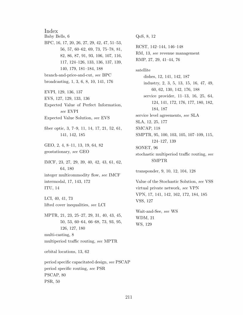
IndexBaby Bells, 6BPC, 16, 17, 20, 26, 27, 29, 42, 47, 51–53,

56, 57, 60–62, 69, 73, 75–78, 81,82, 86, 87, 91, 93, 106, 107, 116,117, 124–126, 133, 136, 137, 139,140, 179, 181–184, 188

branch-and-price-and-cut, see BPCbroadcasting, 1, 3, 6, 8, 10, 141, 176

EVPI, 129, 136, 137EVS, 127, 129, 133, 136Expected Value of Perfect Information,

see EVPIExpected Value Solution, see EVS

fiber optic, 3, 7–9, 11, 14, 17, 21, 52, 61,141, 142, 185

GEO, 2, 4, 8–11, 13, 19, 64, 82geostationary, see GEO

IMCF, 23, 27, 29, 39, 40, 42, 43, 61, 62,64, 180

integer multicommodity flow, see IMCFintermodal, 17, 143, 172ITU, 14

LCI, 40, 41, 73lifted cover inequalities, see LCI

MPTR, 21, 23, 25–27, 29, 31, 40, 43, 45,50, 53, 60–64, 66–68, 73, 93, 95,126, 127, 180

multi-casting, 8multiperiod traffic routing, see MPTR

orbital locations, 13, 62

period specific capacitated design, see PSCAPperiod specific routing, see PSRPSCAP, 80PSR, 50

QoS, 8, 12

RCST, 142–144, 146–148RM, 13, see revenue managementRMP, 27, 29, 41–44, 76

satellitedishes, 12, 141, 142, 187industry, 2, 3, 5, 13, 15, 16, 47, 49,

60, 62, 130, 142, 176, 188service provider, 11–13, 16, 25, 64,

124, 141, 172, 176, 177, 180, 182,184, 187

service level agreements, see SLASLA, 12, 25, 177SMCAP, 118SMPTR, 95, 100, 103, 105, 107–109, 115,

124–127, 139SONET, 96stochastic multiperiod traffic routing, see

SMPTR

transponder, 9, 10, 12, 104, 128

Value of the Stochastic Solution, see VSSvirtual private network, see VPNVPN, 17, 141, 142, 162, 172, 184, 185VSS, 127

Wait-and-See, see WSWDM, 21WS, 129

211