Relative Tagging Ratio

Victor Tarasov

AbstractFor precision measurement of pi0 cross section important to know number of particles in flux.

Additional monitor for flux was Pair Spectrometer (PS) which was counting number of e+e- pairsproduced in target during experiment. Number of this pairs strongly correlate with number of particlesin flux. Relation between number of e+e- pairs in PS and number of particles in flux (in tagger) callsrelative tagging ratio. We supposed that relative tagging ratio is constant run to run.

PS layoutEffective scheme of Pair spectrometer presents on Pic #1. Spectrometer includes dipole magnet

situated downstream of target and vertical scintillation hodoscopes. Hodoscopes make four shoulderssituated from the left and right side of beam direction. Each hodoscope consists of 8-15 planes. Eachplane overlaps side one(except edges) and detects e+e- pairs which were burn in target or beamscanner. Stability of magnet field provides quantity of e+e- pairs during experiment.

Pic #1. Schematic layout of the pair spectrometer.

1

First look at Pair SpectrometerEffective cuts:1) 1st T-counter;2) T-diff<10ns (TRIGPHOTON->trigphoton[i].tdiff<10);3) analyzing files: skim files for PS;4) looking for time difference between tagger (at the beginning of analysis we took data from TRIGPHOTON bank to determinate tagger time, then we took data from TAGM_LR bank which is correct) and PS. result:

Pic #2. Difference between time from tagger and time from PS (before reconstruction,PSHIT bank) for 1st T-counter (bottom – more detail picture).

2

Pic #3. Time difference between time from tagger and time from PS (after reconstruction, PSR bank )for 1st T-counter (bottom – more detail picture).

Should make alignment for each T-counter (we will see follow that they aren't changing run by run).

When we were checking all PS modules for time difference (tagger – PS) we found that some ofthem has “strange/bad” form (see pic #4 and #5-#15)

3

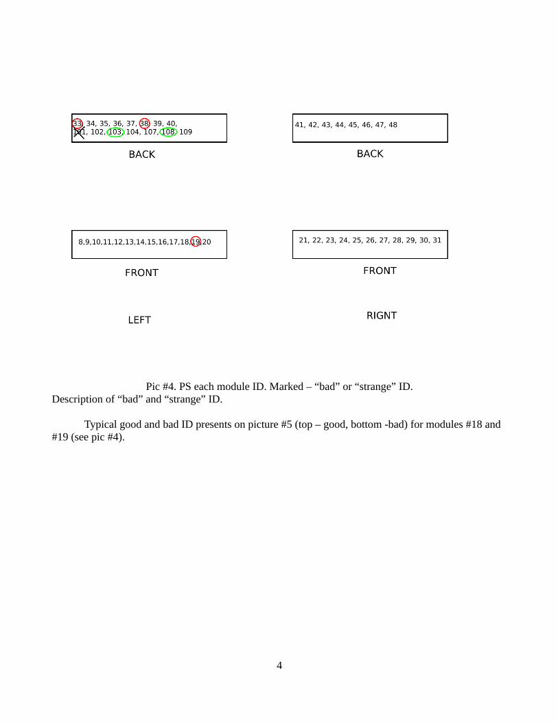
Pic #4. PS each module ID. Marked – “bad” or “strange” ID.Description of “bad” and “strange” ID.

Typical good and bad ID presents on picture #5 (top – good, bottom -bad) for modules #18 and #19 (see pic #4).

4

Pic #5. Typical good (top - id #18) and bad/strange (bottom - id #19).

5

Another deviations:

Pic. #6. Wide peak (ID #8).

Pic#7. Flat backgroun (ID #17). Possible explanation – bad time resolution of this module.

6

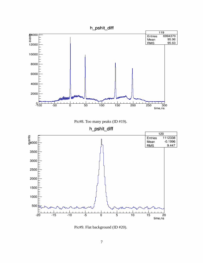
Pic#8. Too many peaks (ID #19).

Pic#9. Flat background (ID #20).

7

Pic #10. Too many peaks (ID #33).

Pic#11. Too many peaks (ID #38).

8

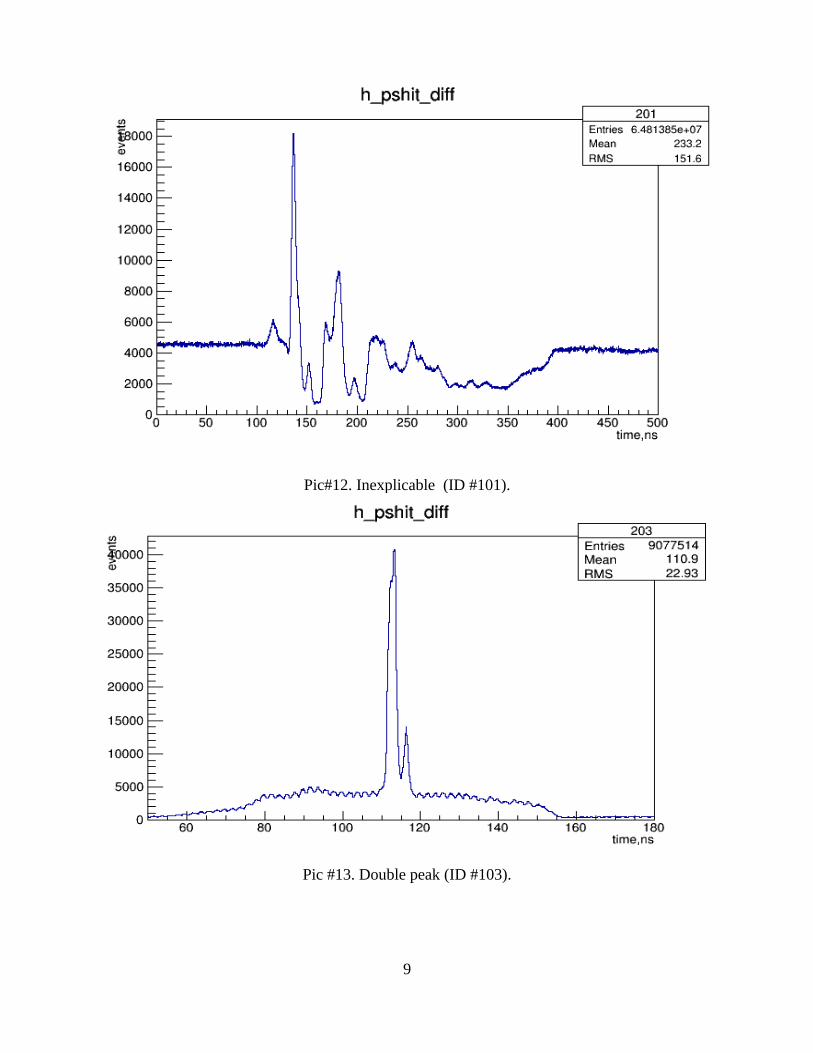
Pic#12. Inexplicable (ID #101).

Pic #13. Double peak (ID #103).

9

Pic #15 Double peak(ID #108).

Picture #16 presents 2d plot which shows time difference versus PS id number.

Pic #16. Time difference versus PS id number.

10

We excluded “bad” and “strange” modules from analysis. Additional modules (#100-108) were also deleted after discussion on weekly PrimEx meeting at March 25th. Remain modules presents on picture #17.

Pic #17. Modules which were stayed in analysis. Red circles – still in analysis with many peaks(analyzing only peak near zero position) but will be removed from analysis soon (see follow).

11

Pic# 18. Time diff (Tagger – PS) for all T-counters and for all(top) and for all without 19, 33, 38 PSmodules(bottom) before reconstruction (PSHIT bank).

12

Check after reconstruction (time difference from PSR bank).

Pic #19. Time diff for all T-counters and all PS-modules after reconstruction for different runs.

13

Alignment for each PS module run by runWe made alignment for all T-counters and for all PS-modules run-by-run (28 tables were written

to DB).

#table Run range

1 64711 - 64743

2 64744 – 64809

3 64810 – 64842

4 64843 – 64844

5 64845 - 64847

6 64848 - 64850

7 64851 - 64855

8 64856 - 64861

9 64862 - 64866

10 64867 - 64885

11 64886 - 64932

12 64933 - 64938

13 64939 - 64947

14 64950 - 64960

15 64961 - 64965

16 64969 - 64973

17 64974 - 64981

18 64982 - 64986

19 64987 - 65008

20 65009 - 65013

21 65014 - 65018

22 65019 - 65032

23 65033 - 65037

24 65038 - 65042

25 65043 - 65048

26 65049 - 65053

27 65055 - 65107

28 65108 - 65112

14

Then we checked reconstruction and have same pic (like pic #18) → reconstruction doesn't work correctly. Should change reconstruction code.

Meeting discussion – remove from analysis modules in red and blue circles:

Pic# 20. Scheme of PS. In blue circles present modules which have no corresponding back PS counters(we exclude them from analysis too).

Reconstruction consist of three parts:1) Overlapping part.2) Front-Back coincidence part;3) Left-Right coincidence part.

Check Overlapping. As we clearly know that modules are overlapping, so we should understandwhich module we need to take into analysis if we will see both “in work” during event.

In picture #21 presents 2-d plot of time diff (tagger-PS) for modules 41 (x axis) and 42 (y axis).Clearly see that we have some regular “physical structure” and it means that overlapping part doesn't work.

15

Pic #21. 2-d plot of time diff for modules 41 (x axis) and 42 (y axis).

So, we assume that we need to remove overlapping part from reconstruction and look on matching modules which situated not close to each other.

Check front-back matching:

16

Pic # 22. Matching of back modules #34 (top) and #35(bottom) with front modules.

17

Pic #23. Matching of front modules #27(top) and #28(bottom) with back modules.

We see that modules 27, 34 and 35 strongly matching with modules 48, 15 and 16 correspondingly. And module #28 matching with many modules. We find that modules #13,14,28,40, 41 matching with many modules during reconstruction, so we removed these modules from analysis.

18

At this point Front-back give us follow picture (see pic #24):

Pic. #24. Modules which stay in analysis after matching front-back modules.

Now we will check idea to matching odd left(front) modules and even right(front) modules (and opposite) and see what we have. For run #64970, for example, for even (bottom) and odd(top) modules we have (see pic # 25).

19

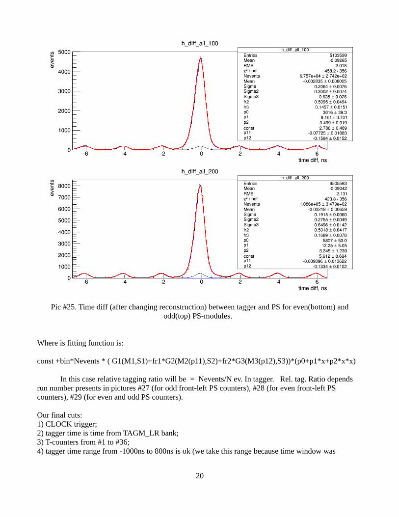
Pic #25. Time diff (after changing reconstruction) between tagger and PS for even(bottom) andodd(top) PS-modules.

Where is fitting function is:

const +bin*Nevents * ( G1(M1,S1)+fr1*G2(M2(p11),S2)+fr2*G3(M3(p12),S3))*(p0+p1*x+p2*x*x)

In this case relative tagging ratio will be = Nevents/N ev. In tagger. Rel. tag. Ratio depends run number presents in pictures #27 (for odd front-left PS counters), #28 (for even front-left PS counters), #29 (for even and odd PS counters).

Our final cuts:1) CLOCK trigger;2) tagger time is time from TAGM_LR bank;3) T-counters from #1 to #36;4) tagger time range from -1000ns to 800ns is ok (we take this range because time window was

20

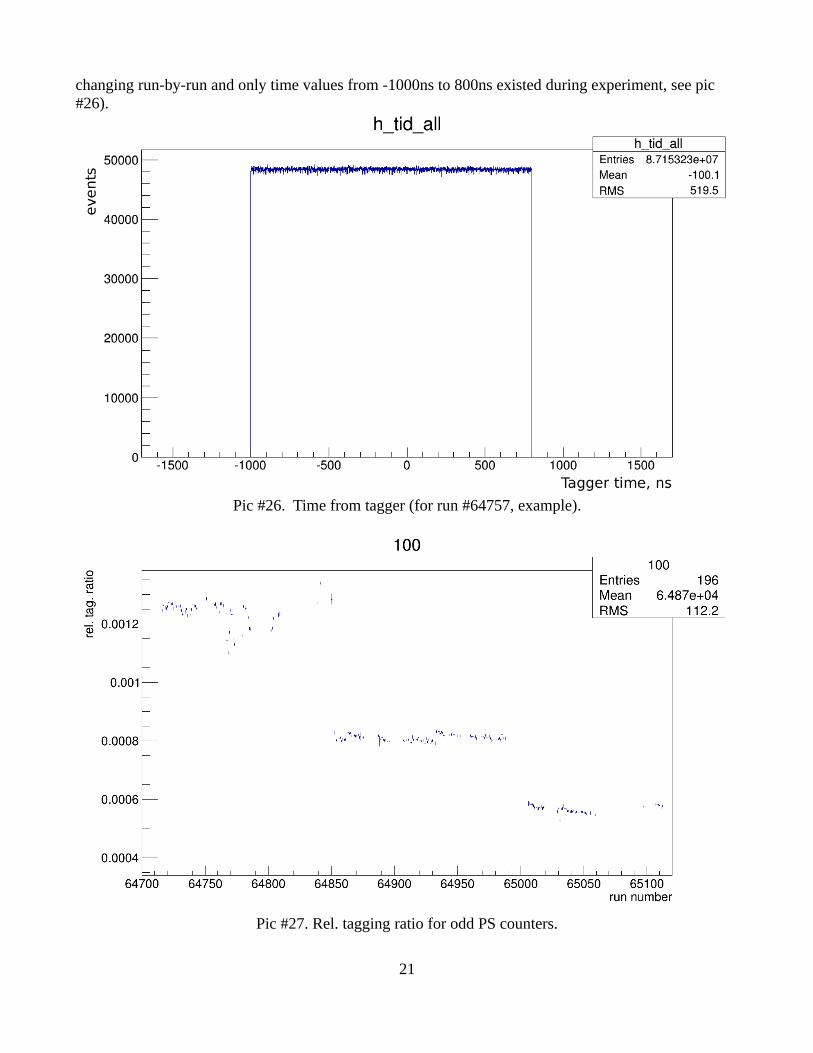
changing run-by-run and only time values from -1000ns to 800ns existed during experiment, see pic #26).

Pic #26. Time from tagger (for run #64757, example).

Pic #27. Rel. tagging ratio for odd PS counters.

21

Pic #28. Rel. tagging ratio for even PS counters.

Pic #29. Tagging ratio for both cases together (pic 26+pic 27).

22

If wee see carefully in pic #27 we can observe that there is some drop of relation in run range near run #64850. Then we look carefully for rel. tagging ratio for each PS counter separatelly and found that for counter #17 exists ratio dramatically drops (see pic. #30) then we remove this module (and module 15 which stayed only one “odd” in left arm) and continue analysis.

Pic #30. Rel. tagging ratio for PS module #17.

And receive:

Pic #31. Rel. tagging ratio for odd PS counters.

23

Pic #32. Rel. tagging ratio for even PS counters.

Pic #33. Rel. tagging ratio for all cases PS counters.

Shift down near run #65000 exist because in that moment Si target was changed to C12 target. That means that number of interaction particles/production particles are different so relative tagging ratio also should be different.

24

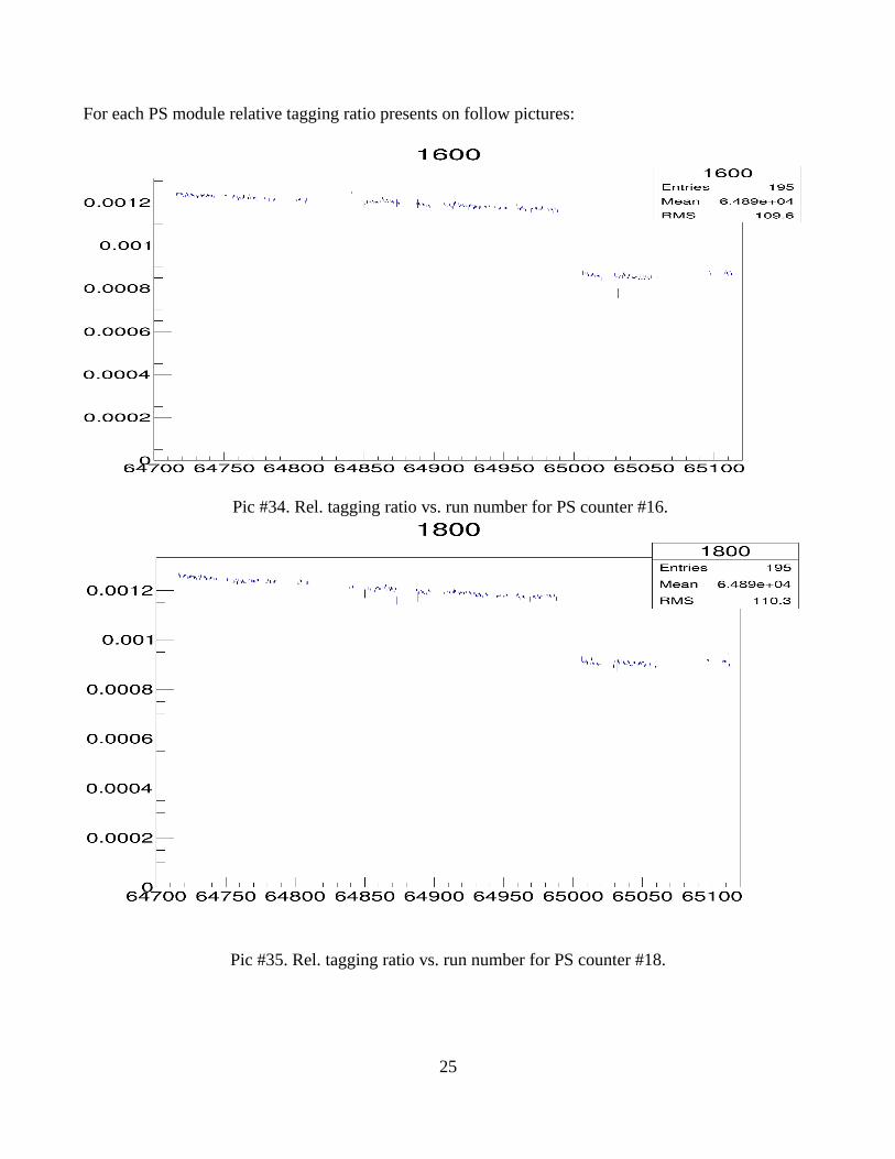
For each PS module relative tagging ratio presents on follow pictures:

Pic #34. Rel. tagging ratio vs. run number for PS counter #16.

Pic #35. Rel. tagging ratio vs. run number for PS counter #18.

25

Pic #36. Rel. tagging ratio vs. run number for PS counter #20.

Pic #37. Rel. tagging ratio vs. run number for PS counter #21.

26

Pic #38. Rel. tagging ratio vs. run number for PS counter #22.

Pic #39. Rel. tagging ratio vs. run number for PS counter #23.

27

Pic #40. Rel. tagging ratio vs. run number for PS counter #24.

Pic #41. Rel. tagging ratio vs. run number for PS counter #25.

28

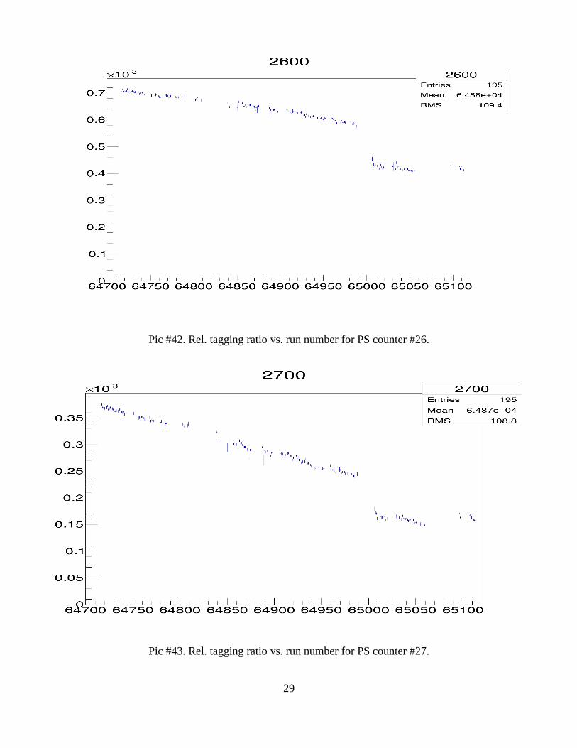
Pic #42. Rel. tagging ratio vs. run number for PS counter #26.

Pic #43. Rel. tagging ratio vs. run number for PS counter #27.

29

ConclusionWe received relative tagging ratio which has a linear structure with slope during experiment. It

is interesting that slope increasing with increasing PS counter number. Nature of this slope still notclear.

30