abstract operational concept and requirements route · pdf filethis study develops an...
TRANSCRIPT

ABSTRACT
This study develops an operational concept and requirements for en route Free Flightusing a simulation of the Cleveland Air Route Traffic Control Center, and developsrequirements for an automated conflict probe for use in the Air Traffic Control Centers.
In this paper we present the results of simulation studies and summarize concepts andinfrastructure requirements to transition from the current air traffic control system tomature Free Flight. The transition path to Free Flight envisioned in this paper assumes
an orderly development of Communication/Navigation/Surveillance technologiesbased on results from our simulation studies. The main purpose of this study is toprovide an overall context and methodology for evaluating airborne and ground-based
requirements for cooperative development of the future Air Traffic Control system.
This study is limited to Free Flight implementation concepts which enable en route UserPreferred Trajectories (UPT). Inherent in these concepts is the notion of intent. We
assume an aircraft is flying a strategic flight plan, or will provide to air traffic controlsome level of intent whenever an aircraft deviates from its intended flight plan. Thoseconcepts of Free Flight operation that do not require any knowledge of aircraft intent
(other than that provided by radar surveillance) may tend to increase controllerworkload. This study assumes that controller workload is the primary limiting factor inmanaging airspace, and that any concept for removing flight restrictions must also
address controller workload. Aircraft intent is essential in this study for enabling moreefficient use of Center resources, off-loading controller workload through automation
concepts such as medium term (10-30 min ) conflict probe and conflict resolutionacross sector boundaries.
https://ntrs.nasa.gov/search.jsp?R=19970012466 2018-05-18T00:24:13+00:00Z


TABLE OF CONTENTS
SECTION
Abstract
Table of Contents
Executive Summary
List of Acronyms
1.0 Introduction and Requirements Summary
1.1 Separation Assurance for Free Flight
1.2 Operational Requirements and Concept Summary
1.3 Free Flight Transition and Mixed Fleet ATM
1.4 Conflict Probe Concepts Analysis
1.5 Technical Requirements for Initial Free Flight
2.0 Separation Assurance and Conflict Alerting Operational Concepts
2.1 Operational Concepts for Initial Free Flight
2.2 Operational Concepts for Mature Free Flight
3.0 Cleveland Center Simulation and Operational Requirements
3.1 Cleveland ARTCC Simulation Model
3.2 Simulation Study Results
3.3 Operational Requirements and Recommended Concepts
PAGE
i
==.
III
vi
X
1
2
5
7
9
12
18
18
24
31
32
37
53
iii

TABLE OF CONTENTS
SECTION
4.0 Conflict Probe Operational Concepts and Technical Requirements
4.1 Conflict Probe Operational Concepts
4.2 Baseline Comparisons of Alternative Concepts
4.3 Conflict Probe Sensitivity Studies
4.4 Technical Requirements for Initial Free Flight
5.0 Conclusions and Recommended Studies
5.1 Operational Concepts and Requirements for Free Flight
5.2 Conflict Probe and Surveillance Requirements for Vertical Transitions
5.3 Cooperative Separation Concept Evolution & Requirements Analysis
6.0 References
Appendix A: Conflict Probe Performance Evaluation Model
A.1 Purpose and Methodology
A.2 Wind Prediction Error Modeling
A.3 Closest Approach Truth Modeling
A.4 Surveillance System / Tracker Noise Modeling
A.5 Estimated Closest Approach Modeling
A.6 Conflict Detection and Performance Modeling
A.7 Monte-Carlo Performance Evaluations
PAGE
60
60
68
74
81
84
85
86
87
88
90
90
90
96
99
104
109
112
iv

SECTION
TABLE OF CONTENTS
PAGE
Appendix B: Conflict Probe Covariance Analysis
B.1 Longitudinal Prediction Error Modeling- Cruise Flight
B.2 Intruder Prediction Uncertainty Modeling
B.3 Covariance Based Thresholding for Conflict Detection
B.4 Predicted Loss-of-Separation Probability
B.5 Predicted Conflict Entry and Exit Times
117
117
120
125
127
128
Nomenclature 133

EXECUTIVE SUMMARY
A number of concepts and methodologies have been proposed for moving towards a
more user oriented air traffic control (ATC) system. The great challenge is to find a
transition strategy for both users and service providers which will provide economic
benefits to justify infrastructure investments, while still accommodating the great
diversity of existing airspace users and their need for ATC services. In this report we
examine several operational concepts for separation assurance which require the
development of new airborne or ground based infrastructure, i.e. conflict probe, alert
zone separation assurance, and use of advanced CNS (Communications/Navigation/
Surveillance) technologies. The central focus of our study is to specify requirements for
conflict probe development and to illustrate its role in transitioning to Free Flight. The
major results of this study are preliminary operational requirements for separation
assurance during the transition to Free Flight, and specification of CNS technical
requirements for infrastructure development in the initial transition toward Free Flight.
The transition path to Free Flight envisioned in this report is based on augmenting the
way that separation between aircraft is achieved in the current ATC system. The
concept utilized in this report is to partition separation assurance into several time
scales, and develop distinct methods for managing separation at each time scale. In
the current system, the sector controller has prime responsibility for separation. System
capacity is limited by the capability of sector controllers to manage separation. The
task of performing separation assurance can be conceptually divided into four primary
time scales: strategic planning, medium term (10 - 30 min) separation assurance, short
term separation, and immediate separation and conflict avoidance. (See Table I,
below.) In our concept, a medium term conflict probe is used to detect and resolve
potential path conflicts prior to the application of short term separation. Similarly,
immediate separation is a function which would be provided by an appropriately
equipped air-crew prior to and during a close encounter between two aircraft.
Table I • Separation Assurance Time Partitioning
Time
Scale
Strategic Planning
Medium Term
Planning & Separation
Short Term
Separation
Immediate
Separation
Current
Separation Method
Central Flow Management
Center Traffic
Management Unit (TMU)
Sector Controller +
Conflict Alert
Air Crew + Traffic
Collision Avoidance
System (TCAS)
Future
Separation Method
Central Flow
Management
Center TMU +
Conflict Probe
Sector Controller +
Conflict Alert
Air Crew + TCAS
+ Alert Zone Monitoring
vi

A conflict probe is vital for Free Flight operations since traffic conflicts can occur
anywhere in a sector with Free Flight, whereas the high workload conflicts today
primarily occur at high density route crossings or merge points. The conflict probe will
identify and alert traffic managers and controllers to conflicts well in advance of a
potential problem, allowing most conflicts to be resolved before the sector controller
needs to become involved. This operational concept has several advantages: (1) we
believe that conflicts can be resolved with smaller perturbations to the flight plan than
with current methods, since more time is available to achieve the needed separation,
(2) the sector controller will be less impacted by high density traffic, allowing the
controller more time to apply separation aids such as future intent displays, and to
respond to airspace user requests, and (3) controllers are less likely to intervene
tactically, allowing users greater benefit from user preferred trajectories.
The advantage of having several redundant systems responsible for separation
assurance is less dependence on one critical subsystem. For example, the conflict
probe does not have to detect all potential conflicts since the sector controller can
easily manage short term conflicts, provided that the number of such conflicts is
reasonably contained. Similarly, airborne based (alert zone) guidance can provide a
high integrity system for managing opposing encounters which are difficult for current
ground based ATC systems.
The methodology employed in our study was to simulate various Free Flight transition
options and evaluate en route encounters parametrically as a function of traffic load.
We developed a simulation of aircraft operations in the Cleveland Air Route Traffic
Control Center over a one day period and benchmarked close encounter statistics for
1995 operations. We then studied the effect of traffic growth over time, and the effect
of implementing various transition options to Free Flight. Figure I summarizes the
methodology that was used to translate the en route encounters obtained for each
transition option into nominal separation parameters. The basis of this process is to
limit the number of encounters at each transition stage to that of the 1995 benchmark.
Cleveland I Encounter --,Center _ Statistics
ISimulation
TFree FlightTransition
Option
CNS Assumptions
* Navigation* Surveillance
Translate Encounters
to SeparationParameters
Conflict Probe
Simulation
Separation
Requirements
Figure I • Methodology to Obtain Requirements for Free Flight Transitions
vii
For each transition option we assume either radar or Automatic Dependent Surveillance
(ADS), and a Required Navigation Performance (RNP) level. The uncertainty inestimating closest approach point of proximate traffic is evaluated with a detailed
conflict probe simulation. Then, separation parameters are derived for each option andtransition time phase, consistent with the CNS infrastructure assumed.
There are four routing / altitude options for transitioning to Free Flight analyzed in our
studies. The first option, denoted Baseline constrains the trajectories by terminal exitand entry conditions to efficiently manage terminal flows, and constrains cruise altitudes
to 1000 or 2000 foot steps, segregated by east or west flying routes. This optionpermits the users freedom in selection of lateral routes and cruise airspeeds, andrequires the least amount of ground and air infrastructure for implementation. The
second option, Baseline Plus RVSM (Reduced Vertical Separation Minimum) reducesthe vertical separation minimum and the vertical steps in cruise altitude above FL290 to
1000 feet. This option permits Baseline flight operations and more efficient use of
cruise flight levels. The third option, En Route UPT (User Preferred Trajectories)removes the constraints on user preferred cruise altitudes, i.e. the user is free to select
preferred altitude and speed cruise parameters as well as lateral path routing. Thisoption permits greater freedom in route selection at the cost of greater ground and airinfrastructure to achieve greatly reduced separations. The fourth option, En RouteUPT Plus RVSM permits En route UPT flight operations with reduced vertical
separations. This option represents a possible end state for mature Free Flight.
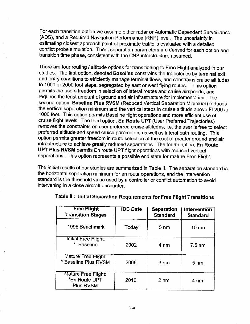
The initial results of our studies are summarized in Table II. The separation standard is
the horizontal separation minimum for en route operations, and the interventionstandard is the threshold value used by a controller or conflict automation to avoidintervening in a close aircraft encounter.
Table II • Initial Separation Requirements for Free Flight Transitions
Free Flight
Transition Stages
1995 Benchmark
Initial Free Flight:* Baseline
Mature Free Flight:* Baseline Plus RVSM
Mature Free Flight:*En Route UPT
Plus RVSM
IOC Date
Today
2OO2
2OO6
2010
SeparationStandard
5 nm
4 nm
3nm
2 nm
Intervention
Standard
10 nm
7.5 nm
5 nm
4 nm
..°Vlll
For the initial Free Flight implementation, the Baseline option is assumed since this
option minimizes the requirements for additional infrastructure. The Baseline optioncan be implemented using existing radar technology for surveillance, whereas we will
need data-link and probably some form of ADS reporting for implementing the other
options. The Baseline option will require precision navigation (RNP-1) equipage in order
to accommodate opposing traffic conflicts. The ground based system will requiresubstantial improvements to the radar tracking system, and implementation of several
Center automation functions in order to accommodate a 4 nm separation standard andto shrink the intervention standard to 7.5 nm. However, there is not a high risk in
implementing these improvements since all the basic technologies are currently inplace. Consequently, we have selected the Baseline flight concept with the abovehorizontal separation parameters for the Initial Free Flight transition.
The next step to Free Flight assumed in Table II is the Baseline Plus RVSM concept,since it has the greatest economic value for users, with the least reduction in separation
parameters to accommodate future traffic growth. However, the Baseline plus RVSMconcept requires that all airspace users flying at or above FL290, including those notflying Free Flight paths, be equipped for RVSM.
The transition to Mature Free Flight is completed using the En route UPT plus RVSMconcept, which again requires reduced separation standards compared with theBaseline plus RVSM concept. However, the horizontal separation standards are much
less severe than those for the En route UPT concept without RVSM, i.e. our studies
show that RVSM should precede the transition to En route UPT. This concept willrequire Alert Zone monitoring to manage same altitude opposing encounters. Thus, thisoption is implemented last in our transition plan to Mature Free Flight.
The emphasis of this report is in developing requirements for the proposed initial step toFree Flight routing, i.e. the ability to fly direct, unconstrained lateral routes while en-route between terminal areas. The main requirement specified for airborne users isan
RNAV system with RNP-1 navigation and path following capability. Some form ofmedium term conflict probe will probably be required at the Air Route Traffic Control
Centers in order to accommodate the increased diversity in path routings. The analysisstudies show that substantial infrastructure changes will be needed at the Centers in
order to support a nominal 20 minute conflict probe. These include development ofenhanced multi-sensor aircraft tracking algorithms, enhanced weather forecasting with
reduced data latency, and implementation of Center automation tools to supportmedium term separation assurance. The medium term conflict probe will require
current path intent for performing trajectory predictions. Consequently, flight path intentmust be updated when path deviations occur, and intent must be validated by real timeconformance monitoring in order to use medium term conflict probe and separation
assurance. The process of updating path intent can be greatly aided by use of air-
ground data-link, i.e. the use of Controller-Pilot Data Link Communications (CPDLC)for path deviation clearances and the use of ADS for verifying current path intent.
ix

LIST OF ACRONYMS
3-D
4-D
ADSADS -BAEEC
AERAARTCCASR
ATCATM
AVPACCDTI
CNS -CPA
CPDLCCTAS
DMEETMS
FAAFMSFP
FTEGA
GICBGPS
HostICAO
IMMIOCITWS
LORANMAPS
MASPSMode-SNAS
OAGRGCSRNAV
RNPRTA
RTCARVSM
Three Dimensional (lat., long., vertical)
Four Dimensional (lat., long., vertical, time)Automatic Dependent SurveillanceBroadcast ADS
Airline Electronic Engineering CommitteeAutomated En Route ATCAir Route Traffic Control Center
Airport Surveillance RadarAir Traffic Control
Air Traffic ManagementAviation VHF Packet Communications
Cockpit Display of Traffic Information
Communications / Navigation / SurveillanceClosest Point of ApproachController-Pilot Data Link Communications
Center- TRACON Automation System
Distance Measuring EquipmentEnhanced Traffic Management SystemFederal Aviation Administration
Flight Management SystemFlight PlanFlight Technical ErrorGeneral Aviation
Ground Initiated Comm-B (for Mode-S)Global Positioning System
The computer used in the ARTCCs for radar and data processingInternational Civil Aviation Organization
Interacting Multiple Model (Tracker)Initial Operating Capability
Integrated Terminal Weather SystemLong Range NavigationMesoscale Analysis and Prediction SystemMinimum Aviation System Performance Standard
Mode Select of Secondary RadarNational Airspace SystemOfficial Airline Guide
Review of General Concept of Separation (ICAO Panel)Area Navigation
Required Navigation PerformanceRequired Time of Arrival
Requirements and Technical Concepts for AviationReduced Vertical Separation Minimums
x

RUCSARP
SSRSTCA
TAAM
TCASTRACON
TWDLUPTVHF
WAAS
Rapid Update Cycle (Wind & Temperature Forecasting)Standards and Recommended Practices
Secondary Surveillance RadarShort Term Conflict Alert
Total Airspace and Airport Modeler
Traffic Alert and Collision Avoidance SystemTerminal Radar Approach ControlTwo Way Data Link
User Preferred TrajectoriesVery High Frequency
Wide Area Augmentation System (for GPS)
xi

1.0 Introduction and Requirements Summary
In today's air traffic control system the freedom to fly user preferred trajectories is
severely limited, given the automation support systems available to controllers. In fact,as demand has grown in NAS airspace, more constraining procedures and flow control
techniques have been implemented in order to keep pace with traffic growth.Procedural restrictions such as en-route spacing and arrival fix spacing, along with flow
restrictions on departure and at critical waypoints are increasingly used today to safelymanage peak traffic flows. However, there are two undesirable effects of this traffic
management system. The first is that the users ability to fly economically optimizedtrajectories, and the timing of the user's flights are greatly constrained by the traffic
management system. The second is that without additional technology for managingtraffic and increased controller productivity, additional airspace limitations will be
needed in the future to restrain the growing traffic demand.
The Free Flight initiative is aimed at evolving airspace management to support trafficgrowth and efficiency of operations, i.e. developing procedures and traffic management
methods which give airline dispatchers and airspace users greater freedom in selectingand modifying flight plans, and some relaxation of flight path constraints when operatingunder airspace flow constraints. The critical element in achieving this goal is controller
productivity. In today's ATC system, the flexibility of the system is determined by theworkload of the sector controllers, i.e. when workload is light, the controllers can moreeasily accommodate user's requests for height and path adjustments, and when
workload is heavy, the controllers can only accommodate basic services for trafficseparation. This report focuses on methodologies for separation assurance which can
off-load the controllers workload or increase controller productivity, and on methods forimplementing Free Flight which are workload efficient for both airspace users andsector controllers. Our study focuses primarily on en route ATC, and the role that
automated conflict probe can play in transitioning to Free Flight.
A number of concepts and methodologies have been proposed for moving towards amore user oriented ATC system. The great challenge is to develop a transitionstrategy for both users and service providers which will enable economic benefits to
justify infrastructure investments, while still accommodating the great diversity of
existing airspace users and their need for ATC services. In this report we examineseveral operational concepts for separation assurance which require the developmentof new airborne or ground based infrastructure, i.e. conflict probe, alert zone separation
assurance, and use of advanced CNS (Communications/Navigation/Surveillance)technologies. The central focus of our study is to specify requirements for conflict
probe development and to illustrate the probe's role in transitioning to Free Flight.The major results of this study are preliminary operational requirements for separationassurance during the transition to Free Flight, and specification of CNS technical
requirements for infrastructure development during an initial transition stage to FreeFlight.
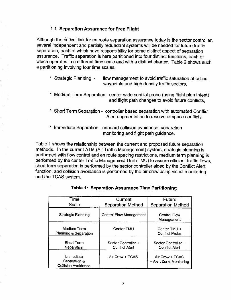
1.1 Separation Assurance for Free Flight
Although the Critical link for en route separation assurance today is the sector controller,
several independent and partially redundant systems will be needed for future traffic
separation, each of which have responsibility for some distinct aspect of separationassurance. Traffic separation is here partitioned into four distinct functions, each ofwhich operates in a different time scale and with a distinct charter. Table 2 shows such
a partitioning involving four time scales:
* Strategic Planning - flow management to avoid traffic saturation at criticalwaypoints and high density traffic sectors,
* Medium Term Separation - center wide conflict probe (using flight plan intent)and flight path changes to avoid future conflicts,
* Short Term Separation - controller based separation with automated Conflict
Alert augmentation to resolve airspace conflicts
* Immediate Separation - onboard collisiOn avoidance, separation
monitoring and flight path guidance.
Table 1 shows the relationship between the current and proposed future separation
methods. In the current ATM (Air Traffic Management) system, strategic planning isperformed with flow control and en route spacing restrictions, medium term planning is
performed by the center Traffic Management Unit (TMU) to assure efficient traffic flows,short term separation is performed by the sector controller aided by the Conflict Alert
function, and collision avoidance is performed by the air-crew using visual monitoringand the TCAS system.
Table 1: Separation Assurance Time Partitioning
TimeScale
Strategic Planning
Medium Term
Planning & Separation
Short TermSeparation
ImmediateSeparation &
Collision Avoidance
Current
Separation Method
Central Flow Management
Center TMU
Sector Controller +Conflict Alert
Air Crew + TCAS
Future
Separation Method
Central FlowManagement
Center TMU +Conflict Probe
Sector Controller +Conflict Alert
Air Crew + TCAS
+ Alert Zone Monitoring
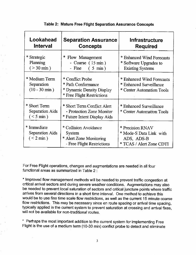
Table 2: Mature Free Flight Separation Assurance Concepts
LookaheadInterval
Strategic
Planning
(> 30 min)
Medium Term
Separation
(10- 30 min)
* Short Term
Separation Aids
(<smin)
* Immediate
Separation Aids
(<2min)
Separation AssuranceConcepts
Flow Management
- Coarse ( 15 min )
- Fine ( 5 min )
* Conflict Probe
* Path Conformance
* Dynamic Density Display
* Free Flight Restrictions
* Short Term Conflict Alert
- Protection Zone Monitor
* Future Intent Display Aids
* Collision Avoidance
System
* Alert Zone Monitoring
- Free Flight Restrictions
Infrastructure
Required
Enhanced Wind Forecasts
Software Upgrades to
Existing Systems
* Enhanced Wind Forecasts
* Enhanced Surveillance
* Center Automation Tools
*.Enhanced Surveillance
* Center Automation Tools
* Precision RNAV
* Mode-S Data Link with
ADS, ADS-B
* TCAS / Alert Zone CDTI
For Free Flight operations, changes and augmentations are needed in all fourfunctional areas as summarized in Table 2 :
* Improved flow management methods will be needed to prevent traffic congestion atcritical arrival sectors and during severe weather conditions. Augmentations may alsobe needed to prevent local saturation of sectors and cdtical juncture points where trafficarrives from several directions in a short time interval. One method to achieve this
would be to use fine time scale flow restrictions, as well as the current 15 minute coarse
flow restrictions. This may be necessary since en route spacing or arrival time spacing,typically applied in the current system to prevent saturation at crossing and arrival fixes,will not be available for non-traditional routes.
* Perhaps the most important addition to the current system for implementing FreeFlight is the use of a medium term (10-30 min) conflict probe to detect and eliminate

potential conflicts prior to the application of short term (tactical) separation. Thisconcept is vital for Free Flight operations since traffic conflicts can occur anywhere in asector with Free Flight, whereas the high workload conflicts today primarily occur atknown route crossing or merge points. The conflict probe will identify and alert trafficmanagers and area controllers to conflicts well in advance of a potential problem,allowing most conflicts to be resolved before the sector controller needs to becomeinvolved. Thus, much of the extra workload during peak traffic can be transferred to thecontroller working the conflict probe, provided that he can directly intervene to resolvepotential conflicts. This operational concept has several advantages: (1) we believethat conflicts can be resolved with smaller perturbations to the flight plan than currently,since more time is available to achieve the needed separation, and (2) the sectorcontroller will be less impacted by high density traffic, allowing the controller more timeto apply separation aids such as future intent displays, and to respond to user requests.
Another function which may be implemented for medium term planning is display of thetraffic load density as a plan view mapping of Center airspace over specified Iookaheadintervals. This function may have several applications for mature Free Flight. Oneapplication is dynamic resectorization of Center airspace to prevent workload saturationat heavily congested traffic areas, i.e. reassignment of controllers to airspace sectorsoptimized for working high traffic loads. Another function may be to apply Free Flightrestrictions such as mandatory waypoint fixes when entering or exiting sectors with hightraffic density.
* Several enhancements to the current system of short-term, tactical separation willprobably be needed for Free Flight operations. One is that decision support tools such
as a future intent display will be needed to implement reduced separation standards.Reduced separations, in turn, will be needed to keep workload from growing
substantially as Free Flight is successively implemented, and as traffic grows over time.Eventually, the process of reducing separations will be limited by inherent time lags inthe control loop, i.e. detecting traffic problems, communicating resolutions to the pilot,and pilot and airplane response times to resolve the problem. This situation is most
critical with opposing conflicts, where the time scales for problem resolution are
compressed. Consequently, the evolution to mature Free Flight will require additionalsystem augmentation to manage opposing conflicts and reduced separationencounters.
* The assumed separation systems above are all ground based. In order to manageclose encounters safely, an airborne system may be needed which will allow the
aircrews in close encounter situations to assume responsibility for separation
assurance, and to provide guidance restrictions immediately preceding and following aclose encounter between two suitably equipped aircraft. Operationally, this meansthere would be a handoff of responsibility between the ground controller and the
aircrews prior to a close encounter between two aircraft, which would persist until theencounter was over. The ground controller would then resume responsibility for
separation assurance. This function has been described somewhat differently by the

Free Flight task force, using the concept of an Alert Zone, which defines a region inspace encompassing a Free Flight aircraft where flight guidance restrictions areimposed whenever an intruder enters the Alert Zone. This function could include an
enhanced TCAS, which would operate somewhat differently than current TCAS
systems, since the system would function to maintain separation standards during anencounter, while current TCAS functions as a backup collision avoidance system.
The implementation of these concepts is dependent on the maturity of the technologies
involved, and availability of supporting infrastructure. Initial Free Flight will probablyinclude medium term conflict probe and separation functions, and various hardware and
software enhancements in the ARTCC's to support this function, most notably a newhost computer system and surveillance system tracker, and enhancements in windforecasting for accurate path predictions. The Alert Zone concept is new, and will
require substantial research and development before it is mature enough for applicationas a means of separation assurance. It is clear however, that the full benefits of Mature
Free Flight will require new CNS technologies onboard, such as precision RNAV or
Flight Management Systems, and an ADS I data link for transferring aircraft position,velocity, and intent information to ground based ATC centers, and to nearby aircraft.
1.2 Operational Requirements and Concepts Summary
An initial simulation study was undertaken to evaluate operational requirements for
separation assurance, based on modeling en route flight operations in a high densityCenter in the current NAS system, and with various Free Flight implementationconcepts. In the simulation studies we evaluated aircraft close encounter statistics for1995 benchmark traffic and for traffic growth to 200% of the 1995 benchmark.
Assuming a nominal 5% per year growth in traffic, then by 2002, the year assumed forinitial Free Flight implementation, traffic will have grown by 140%. By 2010, the yearassumed for mature Free Flight Initial Operating Capability (IOC), aircraft traffic will
have doubled. Thus, we have chosen to evaluate the operational requirements neededfor initial Free Flight using 140% traffic statistics, and the operational requirements for
mature Free Flight using 200% traffic statistics. The methodology in these studies is todetermine separation parameters such that the number of tactical interventions for initial
and mature Free Flight operations does not substantially exceed that for the 1995benchmark.
In the current NAS system, the horizontal separation standard for en route radar control
is 5 nm. Controllers will typically not intervene when the predicted Closest Point ofApproach (CPA) distance of an aircraft pair is more than 10 nm, but will intervene when
the predicted CPA distance is less than 10 nm to assure safe separation consideringpath prediction errors such as radar errors and uncertainty in aircraft intent. The
i In this report we refer to ADS in a generic sense rather than as a specific implementation, i.e. we include Mode-S
Specific Services and Mode-S extended squitters as well as VHF based implementations of ADS.
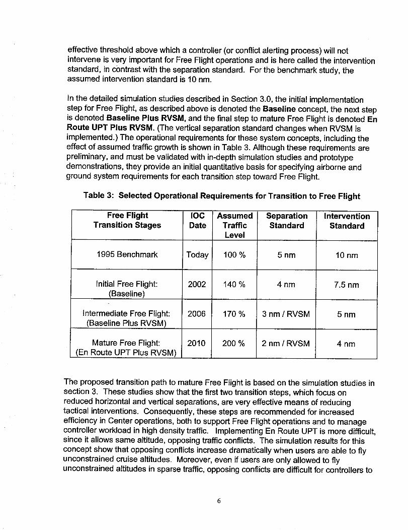
effective threshold above which a controller (or conflict alerting process) will notintervene is very important for Free Flight operations and is here called the intervention
standard, in contrast with the separation standard. For the benchmark study, theassumed intervention standard is 10 nm.
In the detailed simulation studies described in Section 3.0, the initial implementation
step for Free Flight, as described above is denoted the Baseline concept, the next stepis denoted Baseline Plus RVSM, and the final step to mature Free Flight is denoted EnRoute UPT Plus RMSM. (The vertical separation standard changes when RVSM is
implemented.) The operational requirements for these system concepts, including theeffect of assumed traffic growth is shown in Table 3. Although these requirements are
preliminary, and must be validated with in-depth simulation studies and prototypedemonstrations, they provide an initial quantitative basis for specifying airborne and
ground system requirements for each transition step toward Free Flight.
Table 3: Selected Operational Requirements for Transition to Free Flight
Free FlightTransition Stages
1995 Benchmark
Initial Free Flight:
(Baseline)
Intermediate Free Flight:
(Baseline Plus RVSM)
Mature Free Flight:
(En Route UPT Plus RVSM)
IOC
Date
Today
2002
2006
AssumedTrafficLevel
100 %
140 %
170 %
SeparationStandard
5nm
4nm
3 nm / RVSM
2010 200 % 2 nm / RVSM
Intervention
Standard
10 nm
7.5 nm
5nm
4nm
The proposed transition path to mature Free Flight is based on the simulation studies insection 3. These studies show that the first two transition steps, which focus on
reduced horizontal and vertical separations, are very effective means of reducingtactical interventions. Consequently, these steps are recommended for increased
efficiency in Center operations, both to support Free Flight operations and to managecontroller workload in high density traffic. Implementing En Route UPT is more difficult,since it allows same altitude, opposing traffic conflicts. The simulation results for this
concept show that opposing conflicts increase dramatically when users are able to flyunconstrained cruise altitudes. Moreover, even if users are only allowed to flyunconstrained altitudes in sparse traffic, opposing conflicts are difficult for controllers to

manage because of the short time intervals for resolving such conflicts. This optionmay require that the sector controller transfer separation assurance to an air-air basedfunction prior to the occurrence of a close converging encounter, and until such anencounter is completed. (See Section 2.2.2.) This is the purpose of Alert Zone2monitoring and path guidance, i.e. to provide immediate closed loop guidance forseparation assurance to prevent an intruder from penetrating a protection zone aroundthe ownship. The protection zone, as used here, consists of a disk shaped zone with
horizontal radius equal to the horizontal separation standard, and vertical extent (up ordown) equal to the vertical separation standard.
1.3 Free Flight Transitions and Mixed Fleet ATM
From an airspace user's point of view, the most important aspect of Free Flight is the
investment necessary to obtain benefits in terms of increased capacity and flightefficiency. Different users have greatly different needs, which will influenceinfrastructure decisions on airborne equipage. Consequently, the transition path to
Free Flight must have several intermediate stages, in terms of both systemimplementation and user required infrastructure. Table 4 is a transition path to FreeFlight based on the operational requirements in the previous section, which
successively build on earlier steps to incrementally move towards Free Flight, whileallowing users freedom of choice in infrastructure upgrades. (The names of the
incremental stages are shown boldface, underlined in the table.) There are basicallyfour classes of users in positive control airspace and three incremental stages toachieve mature Free Flight in this transition concept:
* Classic, non-FMS aircraft - These aircraft would fly on fixed airways and operateusing ground-based navigation aids, exactly as in today's NAS system. The ATC
services and separation standards would also be maintained as currently, until suchservices are discontinued as the older navigation aids are decommissioned.
* Precision RNAV / FMS aircraft - In the initial stage of Free Flight, these aircraft would
be allowed to fly direct routings and optimal wind routings en-route between a departureexit point and an arrival entry point. (Precision RNAV capability would include aircraftcertified for RNP-1 operations, i.e. GPS, LORAN, and Dual DME based systems.)
Aircraft in this class would be constrained to fly their ground cleared flight plan (orchange their flight plan with ATC approval), and would fly discrete cruise altitude levels
as in the current ATM system. This capability will require integration and fusion of flightplan and surveillance data to perform medium term (-20 minute) flight path predictionsand conflict detection. Aircraft will be monitored in real time for flight plan
conformance, i.e. accurately following the lateral and height profiles in the flight plan.
2 The Alert Zone concept in this report is somewhat different than that assumed by the RTCA Free Flight TaskForce. Our concept uses the intervention standard to define the Alert Zone boundary.

Those aircraft which conform to their intended flight plan will be given reduced
separation minima, and will be subject to less ATC interventions. Those aircraft which
temporarily deviate from the flight plan and are thus not easily predictable for conflict
detection, will be subject to separation minima as in the current system.
Table 4: Airborne Categories for Free Flight Transition Stages
AirplaneEquipage
* Classic,
Non-FMS
* Precision
RNAV / FMS
(RNP -1)
* GPS RNAV /
ADS / RVSM
* 4-D RNAV /
Cooperative
Separation
(Alert Zone)
Operational Concept(Ground Operations)
1995 Benchmark
* 1995 NAS Operations
Baseline Free Flight
Integrated Flight Path &
Radar Data Processing
- Conflict Probe
- Path Conformance
Baseline Plus RVSM
Integrated Flight Path &Radar / ADS Surveillance
- RVSM above FL290
IOC Benefits
* Integrated 4-D Flight
Path +Air / Ground
Surveillance
' Assumes
1995 * Fixed Flight Routes
• Radar Separation
20021 * Reduced Workload
* Increased Capacity
* Partial Free Flight
20061 * Partial Free Flight
* Dynamic Rerouting
* Reduced Separations* More Efficient Cruise
En Route UPT Plus RVSM 20101 * Free Flight Clearances
- User Preferred Profiles
• Reduced Separations
• Priority Scheduling
1996 Consensus on Transition Path for Free Flight
* GPS RNAV / ADS / RVSM aircraft - In the transition stage after initial Free Flight, an
ADS capable air-ground data link will be integrated into the Center operations, and ADS
equipped aircraft will be given additional en-route flight options. These may include
dynamic path routing and automated flight adjustment options such as flight plan offsets
and step-climbs. Integration of radar, ADS, and flight plan data will enable the intended
flight path of the aircraft to be automatically updated for conflict probe and separation
services. The benefits of this transition stage include dynamic flight adjustments and
reduced separation minimums including RVSM (Reduced Vertical Separation Minimum)
above FL 290, enabling additional cruise flight levels. Eventually, all aircraft flying in
high altitude airspace may be required to upgrade to ADS capability, in order to support
reduced separations for airspace capacity and Free Flight compatibility.
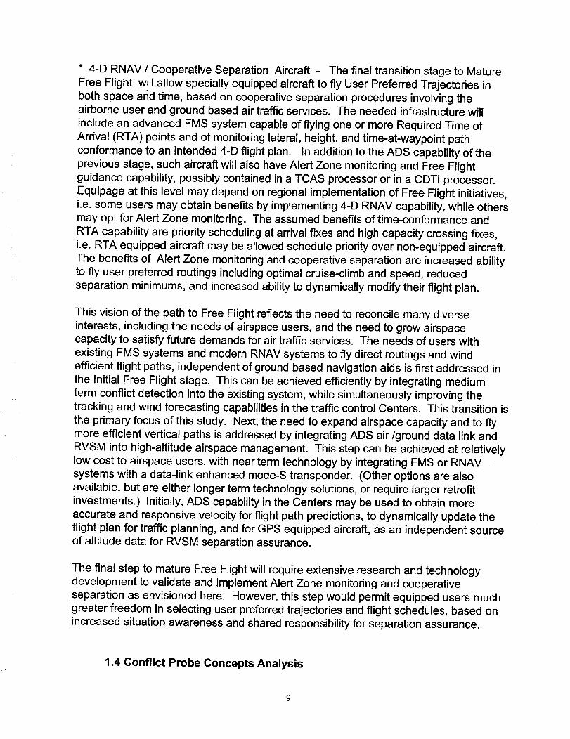
* 4-D RNAV / Cooperative Separation Aircraft - The final transition stage to MatureFree Flight will allow specially equipped aircraft to fly User Preferred Trajectories inboth space and time, based on cooperative separation procedures involving theairborne user and ground based air traffic services. The needed infrastructure will
include an advanced FMS system capable of flying one or more Required Time ofArrival (RTA) points and of monitoring lateral, height, and time-at-waypoint path
conformance to an intended 4-D flight plan. In addition to the ADS capability of the
previous stage, such aircraft will also have Alert Zone monitoring and Free Flightguidance capability, possibly contained in a TCAS processor or in a CDTI processor.Equipage at this level may depend on regional implementation of Free Flight initiatives,
i.e. some users may obtain benefits by implementing 4-D RNAV capability, while othersmay opt for Alert Zone monitoring. The assumed benefits of time-conformance and
RTA capability are priority scheduling at arrival fixes and high capacity crossing fixes,i.e. RTA equipped aircraft may be allowed schedule priority over non-equipped aircraft.
The benefits of Alert Zone monitoring and cooperative separation are increased abilityto fly user preferred routings including optimal cruise-climb and speed, reduced
separation minimums, and increased ability to dynamically modify their flight plan.
This vision of the path to Free Flight reflects the need to reconcile many diverse
interests, including the needs of airspace users, and the need to grow airspacecapacity to satisfy future demands for air traffic services. The needs of users with
existing FMS systems and modem RNAV systems to fly direct routings and windefficient flight paths, independent of ground based navigation aids is first addressed in
the Initial Free Flight stage. This can be achieved efficiently by integrating medium
term conflict detection into the existing system, while simultaneously improving thetracking and wind forecasting capabilities in the traffic control Centers. This transition is
the primary focus of this study. Next, the need to expand airspace capacity and to flymore efficient vertical paths is addressed by integrating ADS air/ground data link and
RVSM into high-altitude airspace management. This step can be achieved at relativelylow cost to airspace users, with near term technology by integrating FMS or RNAVsystems with a data-link enhanced mode-S transponder. (Other options are also
available, but are either longer term technology solutions, or require larger retrofitinvestments.) Initially, ADS capability in the Centers may be used to obtain more
accurate and responsive velocity for flight path predictions, to dynamically update theflight plan for traffic planning, and for GPS equipped aircraft, as an independent sourceof altitude data for RVSM separation assurance.
The final step to mature Free Flight will require extensive research and technologydevelopment to validate and implement Alert Zone monitoring and cooperativeseparation as envisioned here. However, this step would permit equipped users muchgreater freedom in selecting user preferred trajectories and flight schedules, based onincreased situation awareness and shared responsibility for separation assurance.
1.4 Conflict Probe Concepts Analysis
In the initial study phase we examined several different concepts for implementingmedium term conflict detection. These are denoted below Fixed Threshold,
Covariance, and Conformance Bound methods. Each of the concepts examined usesthe same data sources to perform flight predictions, i.e. flight plan intent, radar or ADS
surveillance data, and vector wind forecasts. The concepts differ in the way that thedata is fused into path predictions, and in the way that conformance to the predictedflight path is monitored.
Conventional, strategic flight path predictions use flight plan waypoints and air data
based parameters such as cruise Mach number, together with forecast winds to build a4-dimensional flight path prior to aircraft departure. This flight path is then updated
periodically by removing past waypoints and modifying waypoint times such that thelatest observed aircraft position agrees with the latest observation time. This method of
data fusion and reestablishing conformance of the flight plan may be inaccurate formedium term predictions since it does not use current ground velocity from the
surveillance tracker to perform the flight predictions.
The conflict probes examined in this report use a more accurate methodology to fusesurveillance, wind forecasting, and flight plan waypoints into 4-D flight predictions. We
use flight plan data to determine ground track and altitude profiles for flight predictions,and longitudinal along-track position is determined by projecting the tracker state vectorlongitudinally from the current radar position. The forecast along-track wind is
differenced at intervals along the path to provide an estimate of along-track wind shearfor track segment velocity corrections. This data fusion concept was assumed for all
the medium term conflict probes analyzed in this report. (The Short Term Conflict Alert(STCA) algorithms do not currently use flight plan or wind forecast data, and only usethe tracker state vector to project the flight path forward.)
Three concepts for horizontal plane conflict probe were selected for detailed analysisand study:
* Fixed Threshold Conflict Detection - In this concept, the CPA time and distance of
closest approach are first obtained for each potential path conflict pair. Two thresholdsare used to declare conflicts and non-conflicts, respectively. If the CPA time is outside
a fixed Iookahead interval, or if the CPA distance is larger than an outer threshold(nominally 8 nm for an advanced radar tracker) then the aircraft pair is declared non-
conflicting, and is removed from the list of potential conflict pairs. If the CPA time isinside the probe Iookahead interval (nominally 5 min to 25 min) and if the CPA distanceis less than an inner threshold (nominally 5 nm) then the aircraft pair is declared
conflicting. In order to make the detection process more robust to tracker noise errors,conflicts must be detected two times in a row on two successive probe updates for aconflict alert to be issued for path resolution. (Once a given aircraft has been checked
for path conflicts and found non-conflicting with all other pairs, it is cleared by the
]0

system for unconstrained flight until the next sector exit point is reached, or the aircraft
path is detected out of conformance with the predicted flight path.)
* Covariance Method Conflict Detection - In this concept, error ellipse path uncertaintyregions are computed at the closest approach time together with CPA distance for each
potential path conflict pair. These error ellipses are based on covariance matdx
calculations obtained by modeling tracker surveillance errors, wind forecasting errors,and aircraft path following errors (Ref. 1). The thresholds for declaring conflicts andnon-conflicts are based on the horizontal separation standard and the estimated CPA
uncertainty obtained from the error ellipses. The thresholds with this method are
dynamic and depend on the geometry of the conflict and the time to closest approach.The detection logic for declaring conflicts and non-conflicts is similar to that above, oncethe inner and outer thresholds are computed.
* Conformance Bound Conflict Detection - This concept is a generic version of the
conflict detection method proposed for the AERA-2 program ( Ref. 2, 3). As originally
proposed, each Center maintains a strategic, 4-D flight plan for all aircraft entering intoCenter controlled airspace. This flight plan reflects the current aircraft intent and is keptupdated by path conformance monitoring and surveillance based reconformance if theactual position drifts too far from the predicted flight plan. Conflict detection with this
concept is performed periodically on each aircraft between entry and exit from Center
airspace, and whenever aircraft paths are out of conformance with the intended plan.As applied here, flight predictions are performed using the data fusion methoddescribed above. Fixed size error ellipses are used to model horizontal conformance
bounds for trajectory path following (nominally, 1 nm lateral semi-axis by 2 nm
longitudinal semi-axis). The detection thresholds for this concept are determined by thehorizontal separation standard and the estimated CPA uncertainty obtained from theconformance ellipses. (For details see section 4.1.) Again, the detection logic fordeclaring conflicts and non-conflicts is similar to that above, once the detectionthresholds are computed.
The overall performance of these three methods in detecting horizontal plane conflicts
was evaluated in Monte-Carlo simulations of in-trail, crossing, and opposing pathconflicts. The simulation included the major sources of prediction error including trackernoise, wind forecasting error, and lateral FTE path following error. All three conflictprobe methods were evaluated with the same error sources and geometry, and
common parameters reflecting a 2002 initial operating capability, i.e. a Iookaheadinterval of 20 minutes, separation standard = 4 nm, and intervention standard = 7.5 nm.
The thresholds were tuned as needed to attain a missed detection probability (where noalert is issued for a true conflict) of less than 2 %, and the probability of conflictdetection was evaluated for encounters with approach distance less than 10 nm. Theresults were then aggregated to count the expected number of interventions for eachconflict probe method, and compared to the Benchmark simulation results for 1995
encounters. The results of this study are summarized in Figure 1.
11
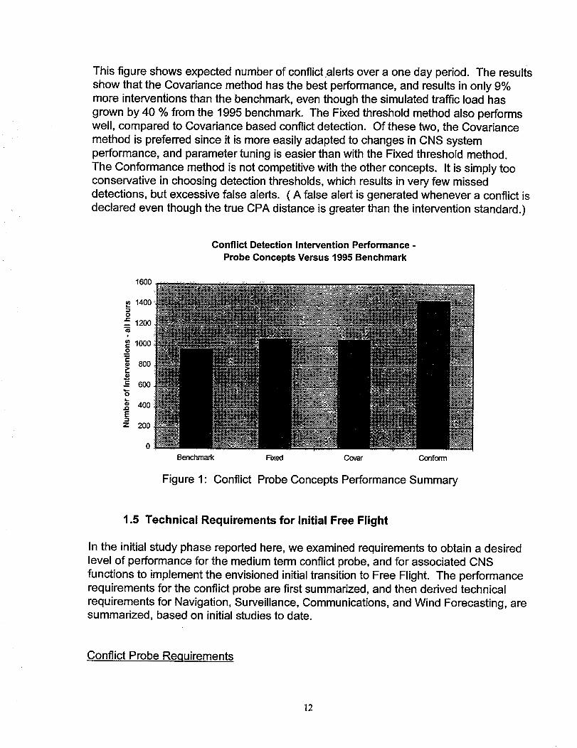
This figure shows expected number of conflict alerts over a one day period. The results
show that the Covariance method has the best performance, and results in only 9%
more interventions than the benchmark, even though the simulated traffic load has
grown by 40 % from the 1995 benchmark. The Fixed threshold method also performswell, compared to Covariance based conflict detection. Of these two, the Covariance
method is preferred since it is more easily adapted to changes in CNS system
performance, and parameter tuning is easier than with the Fixed threshold method.
The Conformance method is not competitive with the other concepts. It is simply too
conservative in choosing detection thresholds, which results in very few missed
detections, but excessive false alerts. ( A false alert is generated whenever a conflict is
declared even though the true CPA distance is greater than the intervention standard.)
Conflict Detection Intervention Performance -
Probe Concepts Versus 1995 Benchmark
1600 __,,_ .. ;ii ..... :;: ......... .....: .._,_;.._._. ._ • ....
p 1400__1200-
_0 600 i400
Benchmark Fixed Covar Conform
Figure 1: Conflict Probe Concepts Performance Summary
1.5 Technical Requirements for Initial Free Flight
In the initial study phase reported here, we examined requirements to obtain a desired
level of performance for the medium term conflict probe, and for associated CNS
functions to implement the envisioned initial transition to Free Flight. The performance
requirements for the conflict probe are first summarized, and then derived technical
requirements for Navigation, Surveillance, Communications, and Wind Forecasting, aresummarized, based on initial studies to date.
Conflict Probe Requirements
12

The main requirements for the conflict probe relate to probability of correct conflict
detection, and to detection time parameters. Key design variables are the probability ofmissed detection, i.e. the probability of not detecting an aircraft pair during the allowed
Iookahead interval, where CPA < separation standard (nominally 4 nm for Initial FreeFlight), and the probability of false alert, i.e. the probability of declaring a conflict alert
on an aircraft pair where CPA distance > intervention standard (nominally 7.5 nm). Wehave used the following initial requirements for our study:
* Missed Detection Probability < 2 %
* False Alert Probability < 6 %
We have initially selected a 2 % rate on missed detection under the assumption thatlow rates are not necessary due to redundancy in separation assurance, i.e. if theconflict probe misses some potential violations, then either the sector controller orConflict Alert automation will detect the violation. The false alert rate is a nominal value
which primarily affects the intervention rate for traffic conflicts. Figure 2 shows nominalconflict probe detection performance for Initial Free Flight. The detection probability isthe observed ratio of conflict detections given 2000 simulated encounters.
==O
¢.1
"6
.O
Covariance Method, Sep Std =4, Int Std = 7.5
Closest Approach Distance (CPA) in nm
Figure 2: Nominal Conflict Probe Performance (Crossing Angle = 90 deg)
The most important time related requirements for conflict probe are the extent of theIookahead interval, the update period between probes, and the mean warning timebetween conflict detection and the predicted conflict. A Iookahead interval of at least 20
minutes prior to CPA time is desired in order to clear an aircraft path through a sector,prior to sector handover. Since the typical time to fly through a sector is on the order of
10 - 15 min (for the simulation described in Section 3), and clearance is desired at least5 min before sector entry, a 20 min Iookahead will generally meet this need. However,
13
25 min Iookahead is desirable and is supported by the covariance method for conflictprobe. The covariance method begins conflict detection when the quality of the CPA
predictions are sufficiently good, i.e. this method will typically begin detecting conflicts
with 12 min to 24 min prediction times, depending on geometry and path uncertainty.The minimum Iookahead time for the conflict probe should coincide with or overlap theIookahead interval for short term Conflict Alert, i.e. nominally 5 minutes Iookahead.
The other conflict probe detection time requirements are:
* conflict probe update period < = 1 min
* mean conflict warning time > = 10 min.
Although most of the conflict probe studies utilized a 2 min update interval, a sensitivitystudy described in section 4.3 revealed that conflict probe detection performance is
more reliable with one minute probe updates, and that mean warning time is somewhatlarger with one minute updates. The conflict warning time is important for conflict
resolutions and at least 10 minutes warning time is assumed in order to minimize pathdeviations to achieve safe separation, and to off-load the workload of the affected
sector controller during peak traffic periods. In practice, one of the goals for the conflictprobe is to achieve 15 minutes warning time, whenever possible. This allows moreoptions for conflict resolution, such as the use of moderate speed and headingdeviations to achieve safe separation during close encounters.
Navigation Requirements
One of the requirements for implementing medium term separation and reduced
separation standards is the necessity to accurately follow the intended flight plan, or todynamically change the flight plan as events require. In order to allow crossing or
opposing encounters with predicted CPA distances less than 10 nm, it will be necessaryfor the airplanes involved to fly precise, predictable RNAV paths. In particular, thenavigation systems for initial free flight aircraft should be capable of precision RNAV
operation equivalent to RNP-I. Precision RNAV capability will be required to meetcollision risk safety requirements for flight path deviations.
Users may be allowed to fly basic RNAV / FMS certified aircraft on free flighttrajectories for some grand-fathered time period, in order to encourage adoption of FreeFlight. However, such aircraft will not qualify for the reduced separation standards
proposed above, and as a result will tend to increase controller workload in the Centers,compared with current jet route operations. The transition to precision RNAV standardsshould be achievable by many modern FMS and RNAV systems, since this level ofaccuracy and integrity should be attainable with dual DME and other multi-sensor
navigation systems, as well as with GPS systems.
14

Surveillance Requirements
The implementation of a medium term conflict probe will require significant changes tothe current surveillance system. The current mode-S Secondary Surveillance Sensors
(SSR) and Airport Surveillance Radar (ASR) sensors are state-of-the-art systems andwill be adequate for ground-based aircraft tracking for the initial phase of Free Flight.
However, the current aircraft trackers embedded in the Host computer system areobsolete, based on legacy software which is difficult to change, and will need to beredeveloped for the conflict probe and other ATC applications (such as the CTAS
terminal approach system). There are two primary problems with these trackers. First,the en route tracking systems use sensor mosaics which determines the single best
radar system to use for aircraft tracking in each mosaic subsector of airspace.Secondly, most U.S. Centers use 30 year old adaptive, alpha-beta-gamma trackeralgorithms which are sub-optimal compared to current state-of-the-art algorithms, and
which are incapable of fusing multiple site, multiple sensor data inputs (Ref. 4). Theproblem with sensor mosaics is that aircraft track positions and velocities may jump
unacceptably as the aircraft transits from one mosaic region to the next. This problemis compounded by the use of legacy trackers which cannot easily differentiate betweenfalse reports, mosaic jumping of position reports, and aircraft maneuvering.
The use of a state-of-the-art Kalman filter tracker supported by modern computinghardware has been proposed to overcome these tracker problems. Such a tracker will
have multi-sensor radar fusion capability for smooth target tracking, and will support
fusion of multi-sensor radar and ADS data for future ATM applications. The followingspecific requirements have emerged from the conflict probe studies in section 4, andfrom an analysis of state-of-the-art tracker capabilities:
* Radar position report accuracy 0.15 - 0.20 nm relative rms error,
* Tracker horizontal velocity accuracy 5 knots rms error (steady state)
* Tracker maneuver convergence time - 20 seconds following maneuver end.
The first requirement is necessary for adequate conformance monitoring and to developaccurate velocity estimates for medium term flight predictions. This requirement shouldbe easily met with modern monopulse radars with rms azimuth errors on the order of
one milliradian or less, since a one milliradian error results in a 0.15 nm crossrangeerror at 150 nm range. However, the older primary radars have rms azimuth errors on
the order of two to three milliradians, and accurate fusion of multiple radars may berequired to meet this requirement. (Ref. 5 discusses multilateration techniques forfusing sensor inputs and test results which illustrate that this capability can be achieved
with older en route radars using multi-site data fusion.)
15

The requirement on velocity accuracy is necessary to obtain accurate estimates ofclosest approach parameters with up to 20 minute path Iookahead. This can be
achieved using a heavily damped tracking filter with long data latency time. However,the tracking filter must also be able to adapt rapidly to tuming maneuvers, i.e. to switchbetween steady state and adaptive maneuver tracking. Both steady state and
maneuver response requirements can be achieved by using modern tracking logicsuch as an Interacting Multiple Model (IMM) tracker (Ref. 6). During vertical transitions,higher accuracy is required even for 10 minute path Iookahead, since the tracker must
estimate ground speed and acceleration states for path predictions.
The requirement on tracker maneuver response time is a 'placeholder' requirementbased on the performance achievable by modern tracking filters in simulation studies.
(Convergence time can be defined various ways, e.g. as the time needed to obtain lessthan a 10 deg heading error after a maneuver is completed.) Fast maneuver
adaptation is needed to support short term separation, and for flight plan conformance
monitoring. It is important to achieve fast adaptation without over responding to falsereports and large sensor errors. Further studies may be needed to validate thisrequirement in terms of improved short term conflict resolution. Good results havebeen reported in meeting this requirement by using either multilateration methods or the
IMM tracker. Another method is to upgrade the SSR hardware, using back-to-backantennas which halve the (en route) radar report interval from 10-12 seconds to 5-6seconds.
Communication Requirements
We do not assume any special voice or data-link communications for Initial Free Flight.In this phase the primary communication between ATC and the aircraft crew will be
performed by VHF voice between the controller responsible for sector separation and
the aircrew. It is assumed that the controller working the conflict probe position hassome direct, but non-obtrusive method of communicating a recommended conflictresolution to the sector controller team responsible for separation assurance. The
sector controller (or assistant) will assess the viability of the recommended resolution
and communicate it to the aircrew. However, this process of implementing mediumterm conflict resolutions is indirect, subject to human error, and not ideal for tacticalcontrol. Consequently, some means of direct data-link communications will be needed
for conflict resolutions in a later transition phase. Further studies are needed to analyzeconflict resolution operational concepts and to derive technical requirements for moreefficient means of implementing conflict resolutions.
Although not required for Initial Free Flight operations, the capability to dynamicallyupdate the flight plan and to communicate path intent will eventually be needed since
medium term separation assurance depends on valid path intent. Thus, capability fordomestic ADS communications will also be needed for later Free Flight transitions.
16

Wind & Weather Forecasting Requirements
The National Weather Service is currently developing an advanced weather prediction
system for the continental U.S., which is called the Rapid Update Cycle (RUC). TheRUC forecasts will use both ground based Doppler radars and airborne observations to
perform detailed 3 hour forecasts for use in aircraft flight predictions. This system willuse 60 km or finer grids and 19 flight levels to perform detailed, mesoscale level
weather predictions throughout continental U.S. airspace. If current implementationschedules are satisfied, the RUC will become available in the en route Centers before
the turn of the century. Thus, we have assumed that the current 12 hour, coarse gridforecasting system will be replaced by the RUC prior to implementation of Initial Free
Flight. The accuracy of the RUC in forecasting winds aloft can be estimated from the
Mesoscale Analysis and Prediction System (MAPS) prototype which has been fieldtested atOdando, FI. and Memphis, Tenn. The field tests show that the RUC will have
an along-track rms mean wind error of about 6 - 9 knots 3 (Ref. 7). Our conflict probestudies show that this level of forecast error will probably be adequate to supportmedium term flight predictions and conflict detection. Consequently, we have assumed
this level of capability as the technical requirement for Initial Free Flight.
s More recent studies have shown that the along track errors associated with 3 hour forecasts may be closer to 10
knots rrns (Ref. 11). However, the RUC forecasts may be improved by using 1 hour forecasts and f'mer grids toachieve the desired forecast accuracy.
17

2.0 Separation Assurance and Conflict Alerting Operational Concepts
The first step in analyzing advanced concepts for Free Flight such as conflict probe and
alert zone monitoring is to specify the operational concept, i.e. how will these systemsoperate, and how will they interface to controllers and pilots to provide separation
assurance. In succeeding sections we will analyze these concepts in greater detail withmodeling and simulation tools, to derive requirements for system implementation. This
discussion is necessary for understanding the context of the analysis. In this sectionwe first discuss operational concepts for Initial Free Flight and then for Mature FreeFlight.
2.1 Operational Concepts for Initial Free Flight_ •
2.1.1 Regional Path Prediction and Load Demand Processing
Restructuring of the hardware and software architecture for Center operations will be
needed to support automation functions such as local flow management, dynamicdensity display of load demand, and automated conflict probe. These operations willrequire systematic development of structured databases to support operationalchanges in Center operations. In this section we briefly describe some core software
structures and databases needed to support medium term traffic planning and conflictprobe automation for Initial Free Flight. The description below is not an operational
concept, but is a conceptual description of software infrastructure for Conflict Probe andother medium term planning functions.
Figure 3 shows a top level flow diagram of the processing functions to support medium
term flight planning and automated conflict probe. (The cylinder shapes representdatabases stored on hard disk, and the rectangles represent processor functions.)
Three dynamic data-bases are needed to perform medium term path predictions: (1) acentral track table containing all of the aircraft tracks operating in or close to Centerairspace, appropriately merged so that each aircraft is represented by one central track
file, (2) a regional weather database containing forecast winds and temperatures over a3-D grid, and (3) a regional flight planning database containing the intended 3-D
waypoints and airspeeds of aimraft flying in Center airspace or which are anticipated toarrive or depart Center airspace in the next (~ 30 min) prediction cycle. Each aircrafttrack in the central track file which has a validated flight plan (in the sense that the
aircraft track is in conformance with its flight plan) is predicted forward over a nominal30 min Iookahead using the data fusion concept described in section 1.4, and stored in
a flight path intent database. The path intent files are subdivided into straight linesegments which represent subsequent short intervals of flight, e.g. 1-2 minute flightsegments. In addition to the internal path predictions, similar path intent files are
communicated from nearby en route Centers whenever an aircraft path is predicted to
18

Weather
ForecastingSystem
o;en eather I
abase _J
I Track I
Regional
Path
Predictions
Flight PlanProcessing
NearbyCenter
Intent Files,¢.................._
-_
-Sector I
abase ._
1Traffic Load
Mapping To "
Airspace Segments
J
Time Ordered
Airspace -_
Occupancy
-.. Table ..;
TMU Applications
I Conflict Probe ICoarse Filtering
Dynamic Density ILoad Mapping
Center Flow
Management
Figure 3: Medium Term Path Prediction and Traffic Load Processing
19

arrive in Center airspace during the prediction period. These path predictions are
repeated at regular intervals, i.e. at nominal one minute update cycles.
In addition to the path prediction files, a systematic means of mapping the predictedtrajectory paths into dynamic airspace traffic loading will be needed to support more
complex Free Flight routings. Conceptually, for each intent path and time segmentwe first establish a mapping PT,I "'> Aj,K,L where PT, I denotes the path predictions for
the T'th time segment and the I'th aircraft track, and Aj,K,Ldenotes a 3-D airspace sub-sector occupied by the aircraft during the T'th time interval. When the mapping process
is completed, then the results are stored in a database ordered by time and airspacesub-sector, i.e. for each time interval T and sub-sector AJ,K,La list of path predictionsegments { PT,_} which occupy that sub-sector is identified and the total number ofaircraft transiting that sub-sector is counted.
The value of the airspace occupancy table is that it provides an underlyinginfrastructure for detecting and resolving medium term traffic load problems and for
coarse identification of potential aircraft conflict pairs. One method for detecting loadproblems is to display dynamic density maps of regional airspace, where the number ofaircraft transiting through each sub-sector over time intervals on the order of 5 - 15 min.
are obtained and displayed graphically to traffic managers. The idea is to managepredicted traffic loads to better utilize Center resources. For example, if an arrival sub-
sector near a terminal area is predicted to overload, then the traffic manager can divertsome of the transiting aircraft in time (via en route holding or airspeed changes), or in
space (via re-routing through adjacent, less congested sub-sectors). The conflictprobe may be used to test the validity of trial flight plan diversions, in such cases, priorto issuing a tactical resolution. A traffic supervisor may also elect to resectorize Center
airspace to concentrate one or several controllers on the congested areas.
There are several alternative methods to perform coarse conflict filtering prior to theapplication of fine resolution conflict detection and alert. One method is to use the
airspace occupancy table to identify potential conflict pairs. Suppose that it is desired
to clear a reference aircraft over a fixed Iookahead interval, e.g. 20 minutes Iookahead.
Then the coarse filter would successively find the sub-sector Aj,K,L transited by thereference aircraft in each subinterval with Iookahead less than 20 min, and then poll allthe aircraft occupying that sub-sector or an adjacent sub-sector to find potential conflict
pairs. This method is much more efficient, for example, than polling all of the otheraircraft in the path intent database to find potential conflict pairs.
It should be noted that the critical step in the above flow diagram is the path predictionprocess. It is important that the accuracy of all the databases supporting this function
be examined and allocated an error budget which will support time critical applicationssuch as fix metering and conflict probe. The primary issues here are the accuracy
requirements on wind forecasting, surveillance error, and open loop trajectory synthesis(for climb and descent trajectory segments). Whether an advanced trajectory synthesissystem such as CTAS, or an advanced ITWAS forecasting system are required
2O

depends on the overall error budget allocation, and the quality of the other subsystemsat the time of deployment.
2.1.2 Conflict Probe Operational Concepts
The basic idea for Initial Free Flight is to use medium term path predictions to identifyand resolve most potential conflicts before they become short term conflicts. Whether
used on a sector basis to clear aircraft paths through a sector, or on a regional basis toprovide more strategic planning, the conflict probe will enable airspace problems to beidentified earlier and solved more efficiently than with the current system. In the AERA
concept (Ref. 3), once an aircraft path has been cleared for flight across a sector orover some Iookahead period, the conflict probe and the path prediction does not need
to be repeated again until the end condition is reached or the aircraft strays from thepredicted path. We have also adopted this concept, except that the time interval forrepeating the conflict probe should be some fraction of the Iookahead interval for
conflict detection, i.e. the conflict probe should be repeated at least twice over a 20minute period, since the accuracy of path prediction increases significantly as theprediction time is decreased from 20 to 10 minutes.
The flight plan, which describes aircraft path intent and anticipated waypoint times, isessential for medium term flight predictions. However, short term deviations such aspath offsets, heading vectors from the nominal path, and temporary altitude transitions
need to be integrated into the planning and monitoring process whenever possible for
the conflict probe to be effective. (Without a currently valid flight plan, flight predictionsare not possible and only short term monitoring and control based on radar surveillanceis feasible.) We shall designate the original, unmodified flight plan as the primary flight
plan, and deviations from this plan as an alternative flight plan if this plan is currentlyactive, or as a trial flight plan if this is a requested option by the air-crew or by a groundcontroller for solving an airspace problem. We here designate the position which
monitors medium term conflicts as the planning controller. (It is assumed that theplanning controller and the sector / radar controller are different positions.) The
planning controller will have responsibility for medium term flight planning andidentifying path resolutions to solve potential airspace conflicts. The planning controllerwill need considerable automation support in addition to the conflict probe,
in order to assure that the aircraft is following the active flight plan (conformancemonitoring), to aid the controller in validating separation with a proposed trial plan,and in activating an alternative flight plan when a dynamic path change is needed.
However constructed, the active flight plan is- monitored at each radar scan forconformance with the predicted flight path established by the conflict probe, i.e. the
predicted lateral and ground track are determined by the active flight plan and thepredicted longitudinal position is determined from the aircraft state vector at the last
probe time. The horizontal conformance bounds on the trajectory can be viewed aseither uncertainty ellipses or as lateral and longitudinal parallelograms centered on the
predicted path. In this report we assume that the conformance bounds are elliptical
21
regions, since this simplifies the analysis for detecting aircraft conflicts, and iscompatible with our covariance analysis for modeling trajectory prediction uncertainty.
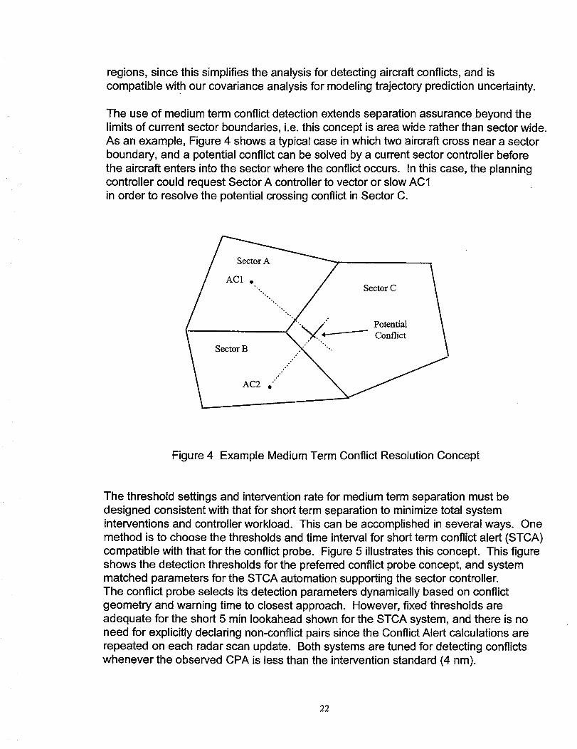
The use of medium term conflict detection extends separation assurance beyond thelimits of current sector boundaries, i.e. this concept is area wide rather than sector wide.
As an example, Figure 4 shows a typical case in which two aircraft cross near a sector
boundary, and a potential conflict can be solved by a current sector controller before
the aircraft enters into the sector where the conflict occurs. In this case, the planningcontroller could request Sector A controller to vector or slow AC1
in order to resolve the potential crossing conflict in Sector C.
AC2 .'"'"''""
Figure 4 Example Medium Term Conflict Resolution Concept
The threshold settings and intervention rate for medium term separation must bedesigned consistent with that for short term separation to minimize total systeminterventions and controller workload. This can be accomplished in several ways. One
method is to choose the thresholds and time interval for short term conflict alert (STCA)
compatible with that for the conflict probe. Figure 5 illustrates this concept. This figureshows the detection thresholds for the preferred conflict probe concept, and systemmatched parameters for the STCA automation supporting the sector controller.The conflict probe selects its detection parameters dynamically based on conflict
geometry and warning time to closest approach. However, fixed thresholds areadequate for the short 5 min Iookahead shown for the STCA system, and there is noneed for explicitly declaring non-conflict pairs since the Conflict Alert calculations are
repeated on each radar scan update. Both systems are tuned for detecting conflictswhenever the observed CPA is less than the intervention standard (4 nm).
22

7
E¢..,- 6
O" 5¢/)
.=
<_ 4
o3
Conflict Probe Thresholds - Del_Psi=30 deg
nflict -
4---STCA _ _ Conflict Probef I I
0 5 10 15 20 25
Iookaheadtime in min
Figure 5 Conflict Probe and STCA Thresholds versus Lookahead Time
Of greater concern is the capability of controllers to provide oversight on theseparations provided by the conflict probe. Additional automation tools will be needed
to support reduced separation standards. Figure 6 shows a concept which uses
predicted conflict uncertainty as a decision aid for the planning and sector controllers.In the event that the predicted separation between two aircraft is questionable, acontroller will be able to call up an overlay display which shows the predicted intruderpath relative to a reference aircraft. The reference aircraft in the figure has displayed
the radial separation standard and the intervention standard for comparison with the
predicted intruder path. The predicted intruder path relative to the reference aircraftand the path uncertainty are displayed by the dotted line overlays. In this figure, theintruder is climbing through the reference aircraft flight level. The time interval when
vertical separation is lost is shown in heavy double lines. For medium term separation,the bounding lines for intruder containment can be at the 95% probability level or lower,
since a reasonable level of missed detections is allowed, whereas the bounding linesfor short term separation may be at the 99.9 % level or higher, since the sector
controller is responsible for assuring separation greater than the minimum. Thecontrollers should intervene if any portion of the heavy line containment boundary
intersects with the reference aircraft inner circle (protection zone), and should notintervene if the intruder containment region lies outside the intervention ring. In the
figure below, the decision to intervene or not is up to the controller, since the predictedCPA lies between the separation and intervention standards.
23
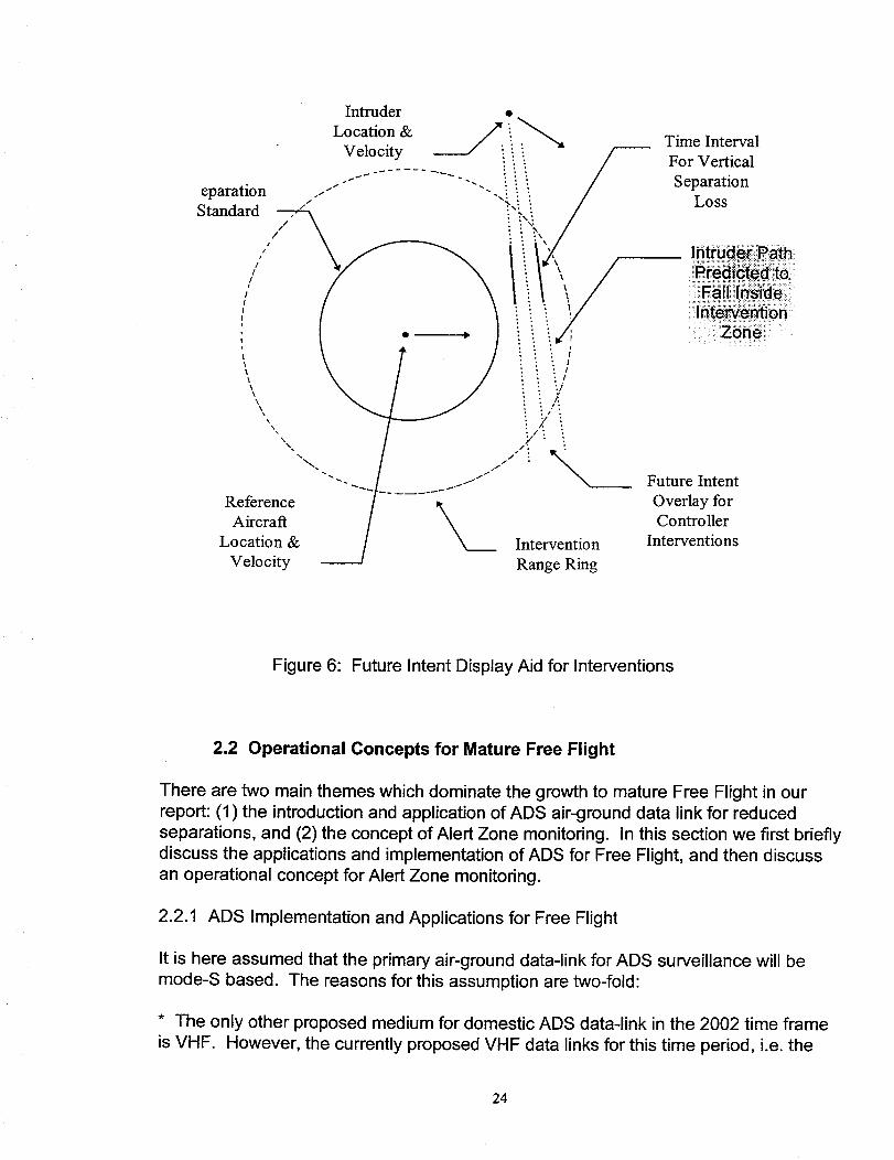
Intruder •
Location& ______:. i "" _Velocity /
eparation ..--"" """-.i_ ! /Standard_ _.'!.,! /
/ \ -" /
,/ _ :
L i " I
', \ / / !'t,;
%%
Reference
Aircraft
Location &
Velocity
./:
Intervention
Range Ring
Time Interval
For Vertical
SeparationLoss
Future Intent
Overlay forController
Interventions
Figure 6: Future Intent Display Aid for Interventions
2.2 Operational Concepts for Mature Free Flight
There are two main themes which dominate the growth to mature Free Flight in our
report: (1) the introduction and application of ADS air-ground data link for reduced
separations, and (2) the concept of Alert Zone monitoring. In this section we first briefly
discuss the applications and implementation of ADS for Free Flight, and then discuss
an operational concept for Alert Zone monitoring.
2.2.1 ADS Implementation and Applications for Free Flight
It is here assumed that the primary air-ground data-link for ADS surveillance will be
mode-S based. The reasons for this assumption are two-fold:
* The only other proposed medium for domestic ADS data-link in the 2002 time frame
is VHF. However, the currently proposed VHF data links for this time period, i.e. the
24
AVPAC radio and the multiplexed digital voice / data-link radio will not have sufficient
bandwidth for routine ADS surveillance, where report intervals of ten seconds or lessmust be sustained. By contrast, report intervals of one second or less are sustainable
using mode-S squitter (Ref. 8) broadcasts (ADS-B).
* Most of the infrastructure for mode-S data-link currently exists, i.e. there are over 140
deployed mode-S ground sensors, and thousands of installed mode-S transponders,since all of the TCAS-II equipped planes carry a mode-S transponder. Moreover, lowcost ($4000) mode-S transponders are currently available for GA aircraft. Since data-
link capability is built into the mode-S system, the current generation of mode-S
transponders can be upgraded to support ADS-B and TWDL capability.
The design and formatting of mode-S message formats for ADS is currently underdefinition in various ICAO, AEEC and RTCA standards committees. However, we can
anticipate several capabilities based on current draft SARP and MASPS documents.
The first is that all equipped aircraft will broadcast GPS 'squitters' containing theirposition and velocity states for air-air and terminal area air-ground applications.
However, the GPS squitters may have limited range, and will not be directly applicablefor en route air-ground applications. Consequently, ADS for en route applications will
probably be based on the mode-S radars and on Ground Initiated Comm-B (GICB)requests for information as an aircraft comes within the current scan radar beam. (It is
also possible to transmit unsolicited air-ground messages after the standard SSR replyon each scan, in order to transmit ADS broadcast messages at longer ranges.)
The following types of messages useful for Free Flight applications can be requestedfrom ground sensors using mode-S special services message formats (Ref. 9):
* ground and air referenced position and velocity states
* pressure altitude and altitude rate
* geometric altitude and altitude rate
* aircraft wind and temperature states
* aircraft future intent
- 4-D waypoints including waypoint times
aircraft short term intent
vertical intent parameters including altitude target and time-to-level-offhorizontal turn parameters including selected ground track and time-to-turn.
There are many potential applications for ADS to improve future ATC Center
operations. The most significant for transition to mature Free Flight are:
25

* Monitoring of ADS velocity vector and ADS / Radar data fusion :
One of the limiting factors in controlling aircraft tactically today is the uncertainty in shortterm aircraft intent, since the aircraft velocity state is not monitored, but derivedindirectly by filtering noisy radar position measurements. When an aircraft deviates
from its intended flight plan, it can take many scans to detect the deviation from radar
measurements. ADS velocity monitoring will enable immediate detection of flight plandeviations, and immediate confirmation of tactical vectoring for separation assurance.
This capability will be needed in mature Free Flight to support reduced separationstandards.
The other area where ADS monitoring may be needed is to support medium term pathpredictions in climb and descent flight phases. The sensitivity studies in Section 4 show
that conventional radar tracking during periods of non-constant velocity flight (such asclimb and descent phases) may not support adequate Iookahead periods for efficient
resolution of potential conflicts. Aircraft path observability is greatly improved with ADS
monitoring and its use in climb and descent predictions may be essential for reducingseparation conflicts during vertical flight. Since the vast majority of close encounters inInitial Free Flight will involve climbing and descending aircraft, this is an area that needsclose attention in future research studies.
* Monitoring of Geometric Altitude for RVSM :
One of the primary goals for efficient high altitude flight is the ability to fly at 1000 foot
flight levels above FL290, rather than the current 2000 foot flight levels. The ability tofly 1000 foot flight levels will become a reality in 1997 for North-Atlantic flights inoceanic airspace. However, the methods used to support RVSM in the Atlantic are
expensive for both airborne users and ATC service providers. The problem is that in
the current system there is no independent cross-check on baro-altimeter accuracy. Aspecial uplooking radar sensor is being developed for North-Atlantic flights that will
check the altimeter accuracy as aircraft exit into the oceanic track system. However, bythe year 2000, the Wide Area Augmentation System (WAAS) will be implemented over
NAS airspace, and GPS based geometric altitude will be available with sufficiently highaccuracy, integrity and availability for use in vertical separation assurance. Whether
geometric altitude is used directly for vertical separation above FL290, or simply as anindependent cross-check of baro-altimeter accuracy will be decided in the future.
However, it appears to be a cost effective method of implementing RVSM for lowercapability GA aircraft and for altimeter cross-checks at the ATC Centers. We assume
that ADS broadcast of GPS altitude and altitude rate will become a required capabilityfor aircraft flying above FL290 during the transition to mature Free Flight.
* Updating and Validation of Flight Plan Intent :
One of the operational problems which arises with medium term separation methods is
that of updating the flight plan to reflect current conditions. If a pilot in an RNAV or FMS
26

airplane, for example needs to make a weather based adjustment to the flight plan inconcurrence with the sector controller, then the pilot will add or change waypoints toimplement the new flight plan. Without data link capability, the ground based flight planis then invalid until either updated manually or until the aircraft returns to the previousflight plan. With ADS data link capability, the ground can update or validate the flightplan periodically by requesting future aircraft waypoints and checking them against thecurrent flight plan. This process will assure consistency between the aircraft intendedflight plan and the ground based flight plan.
* Broadcasting Aircraft Equipage Capability for Mixed Fleet Separation :
We have proposed in Table 3 reduced separation standards for appropriately equippedaircraft as the transition to mature Free Flight occurs. However, in a mixed fleet
environment, the separation standard of the least capable aircraft should be used in anencounter. This may be accomplished in mature Free Flight by broadcasting aircraft
minimum separation capability. In particular, this is needed for Alert Zone monitoring sothat an appropriate separation standard is applied for potential encounters.
2.2.2 Operational Concepts for Alert Zone Monitoring
One of the fundamental limits of ground based separation is the amount of time it
requires to intervene tactically to achieve separation. Some of the problem with current
systems is due to sensor limitations which result in poor observability of aircraft intent.Even if this problem is overcome using ADS monitoring, the problem of time lags inresolving conflict encounters will remain. One way to overcome this limit is to transferresponsibility for separation assurance from the ground controller to the pilot, with a
means provided the pilot for high integrity, high accuracy situation awareness. Weassume in the following that all aircraft flying in mature Free Flight airspace will bebroadcasting GPS squitters containing their current position and velocity states, to
provide such situation awareness for airborne systems. Alert Zone monitoring is aconcept for specially equipped aircraft to detect close encounters, and to provide
autonomous guidance for safe separation during an encounter interval. The Alert Zone
is the region where the guidance cues are active, and is specifically needed to provideseparation assurance in same altitude, opposing encounters.
Alert Zone monitoring will require some kind of hand-off of separation responsibility
from ATC to the pilot and back to ATC when an encounter is completed, in order for
ATC to accept reduced separations such as those shown in Table 3. Conceptually, thismay be accomplished as shown in Figure 7. At position (1) the conflict probedetermines that an opposing encounter between AC1 and AC2 will occur, and alerts anappropriate sector controller. At position (2), the squitters from AC2 are detected and
the pilot is notified that AC2 will be entering his aircraft Alert Zone. The pilot thenactivates Alert Zone monitoring which sends a message to the sector controller to the
effect that aircraft AC1 is now providing self separation. At position (3), the Alert Zone
2?
monitor determines that the two aircraft have established safe separation and are ondiverging paths, and deactivates Alert Zone monitoring, freeing the pilot for other tasks.A message isthen sent to the controller to the effect that separation assurance for AC1
is being returned to the controller. If neither aircraft activates Alert Zone monitoringwithin a specified time before closest approach, then the sector controller will intervene
as necessary to assure separation.
(2)
(1) Conflict Probe ProvidesProvisional Clearance
for Opposing Encounter
ACl
O osm _ " * _
AC2
(1)
Figure 7: Cooperative Separation Concept for Alert Zone Monitoring
In our concept, an intruder enters the Alert Zone when the predicted CPA of the intruderis less than the intervention standard, the vertical separation is less than the minimum
allowed, and the time to CPA is less than some threshold value, say two minutes toCPA. The aircraft remains in the alert zone until the aircraft paths diverge and the
intruder range is greater than the intervention standard or vertical separation isachieved. Guidance path restrictions are continuously displayed in the Alert Zone, orearlier if the pilot has previously activated Alert Zone monitoring. The guidance
restrictions prevent the pilot from heading in a direction which will intercept theintruder's protected zone. Figure 8 illustrates this concept. In the rare event that the
predicted CPA becomes less than the separation standard (plus a small buffer) then theownship path will be between the two dotted lines in the figure and the Alert Zonemonitor will issue a resolution advisory (path heading / speed change) to achieve safe
separation, and will send a cooperative advisory to the intruder, and an alert to theground controller. For FMS equipped aircraft, guidance restrictions would be displayed
on the navigation display and interfaced to the flight management system.
28

Ownship Path
Restriction Zone _X':
Intruder Position and
Protected Zone
°,• ."
....../_i_. "
.: :i_Jiiii_i_.. :"
_______ Ownship Position
Relative to Intruder
Ownship Path
Relative to Intruder
Figure 8: Alert Zone Guidance Restrictions
Now the operational concept can be summarized in terms of the following procedures:
(1) Whenever another aircraft becomes observable, the time to closest approach,
time to flight level crossing, and CPA distance are monitored. If the closest
approach exceeds the intervention standard, or vertical separation is assured,
then the Alert Zone monitor remains in the background.
(2) If the CPA distance is predicted to be less than the intervention standard and
vertical separation is not assured, then the pilot is alerted and can take
responsibility for path separation, i.e. the controller is notified and the Alert Zone
monitor will continuously display guidance restrictions. In the event that this
CPA condition persists and the Alert Zone is entered, the monitor will notify thepilot and display guidance restrictions until Zone exit.
(3) If the intruder enters the Alert Zone, and the ownship path is in the restricted
zone, i.e. the predicted CPA is less than allowed for safe separation, then the
system will issue a horizontal resolution advisory to achieve the required
separation and send a complementary advisory to the intruder aircraft. If this
fails to be effective due to intruder maneuvering or other causes, then the TCAS
system will issue a vertical resolution advisory to prevent path collision.
29
This concept of airborne separation is cooperative in the sense that the intruder aircraft
must be able to broadcast position and velocity state information for Alert Zone
monitoring, and must be able to receive some form of cooperative guidance restriction,
i.e. the Free Flight aircraft may broadcast a message which is translated into an aural
warning onboard the intruder aircraft, and into preventive guidance cues for CDTI
equipped aircraft. It should be observed that path resolutions are not limited by 'rules-
of-the-road' which favor right hand turns by both aircraft involved in crossing or
opposing encounters. Although 'rules-of-the-road' procedures are simple to understand
and implement, they are not compatible with multiple aircraft encounters, or with mixed
equipage encounters where one aircraft has superior situation awareness of the
encounter geometry.
Other concepts have been proposed for implementing Alert Zone monitoring. The
above concept was conceived as a methodology which is reasonably simple to
implement for mature Free Flight (provided that all nearby aircraft broadcast GPS
squitters), and which maintains the same separation parameters for ground and
airborne separation assurance, providing consistency between medium term, short
term, and airborne separation systems.
3o

3.0 Operational Requirements for Separation Assurance
This section isconcerned with obtaining numeric requirements for separation
assurance so that tactical interventions do not grow excessively as Free Flight isprogressively implemented. Most tactical interventions in the current ATC system are
either for separation assurance or to manage traffic flows for high capacity operations.In order to move towards Free Flight, new concepts and implementing technologies willbe needed to keep tactical interventions and controller workload at manageable levels.
One of the main concepts is to implement systems which will permit reducing the size ofthe aircraft protection zone, eliminating the need for a substantial proportion of en routeinterventions. A second concept is to use automated conflict probes to determine
which aircraft need to be moved due to potential path conflicts. Aircraft paths will notbe changed unless there are predicted path conflicts or flow restrictions are going to beviolated.
There are four routing / altitude options for transitioning to Free Flight analyzed in the
studies below. The first option, denoted Baseline constrains the trajectories byterminal exit and entry conditions to efficiently manage terminal flows, and constrains
cruise altitudes to 1000 or 2000 foot steps, segregated by east or west flying routes.This option permits the users freedom in selection of lateral routes and cruise
airspeeds, and requires the least amount of ground and air infrastructure forimplementation. The second option, Baseline Plus RVSM (Reduced Vertical
Separation Minimum) reduces the vertical separation minimum and the vertical steps incruise altitude above FL290 to 1000 feet. This option permits Baseline flight operationsand more efficient use of cruise flight levels, at the cost of additional airborne avionics.
The third option, En Route UPT (User Preferred Trajectories) removes the constraintson user preferred cruise altitudes, i.e. the user is free to select preferred altitude and
speed cruise parameters as well as lateral path between terminal exit and terminalarrival points. This option permits greater freedom in route selection at the cost of
greater ground and air infrastructure to achieve greatly reduced separations. Thefourth option, En Route UPT Plus RVSM permits En route UPT flight operations withreduced vertical separation minimums. This option represents a possible end state for
mature Free Flight. Other routing options are possible, but the four selected providegood insight into the trades between increased route choices and the CNS
infrastructure needed to support them.
The basis of this task is a simulation of the aircraft operations in the Cleveland ARTCC(Air Route Traffic Control Center) over a one day period. Section 3.1 describes this
simulation model. The simulation studies using this model are summarized inSection 3.2. These studies include benchmarking the close encounter or close
proximity statistics for 1995 operations, and showing the time phased growth inencounters due to traffic growth over time, and due to implementation of successive
transition steps to Free Flight. Operational requirements for Free Flight transitions arethen derived in Section 3.3, based on the simulation results in Section 3.2.
3]

3.1 Cleveland ARTCC Simulation Model
This section describes the U.S. Cleveland Air Route Traffic Control Center (ARTCC)
simulation model. This model was developed using the TAAM (Total Airspace andAirport Modeler) simulation. The purpose of the model is to simulate air traffic for an
en route center and count the number of close encounters between aircraft pairs.Section 3.1.1 describes the benchmark model and Section 3.1.2 describes the
methodology used in the study.
3.1.1 Cleveland ARTCC Model Description
The U.S. Cleveland ARTCC was chosen to represent a high altitude en route trafficregion with high density traffic peaks. The ten sectors in this region are shown in
Figure 9. These sectors start at FL240 and include the airspace above FL240. The"current" air traffic for the region was obtained from the Official Aidine Guide (OAG), forthe day August 1, 1994. Any flight that has a direct route through the ClevelandARTCC was selected for the study. The total number of flights simulated is 4,555. Of
these 1,121 are inter-flights or flights between airports near or in the ARTCC region,
2,593 are arrivals or departures to one airport near or in the region, and 841 areoverflights.
IZOB181
IZOB281
ZOB361
IZOB46] ZOB48
IZOB571
IZOB671
Figure 9: Sectors Used in the Cleveland ARTCC Study
32
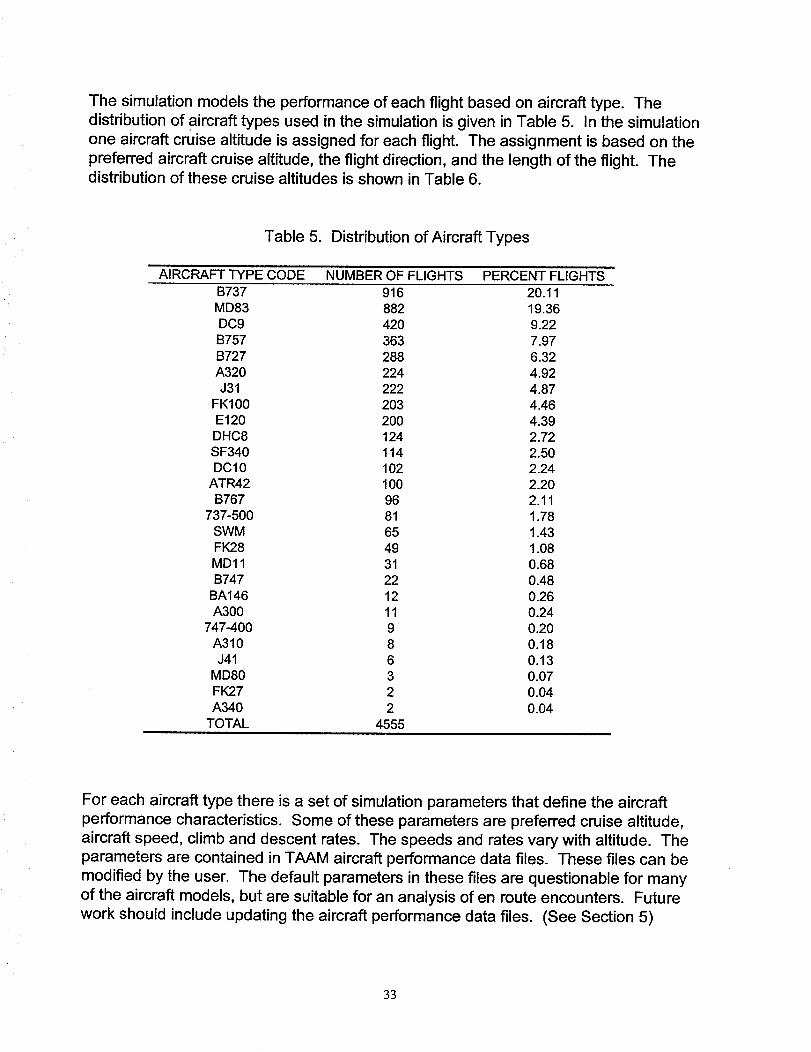
The simulation models the performance of each flight based on aircraft type. The
distribution of aircraft types used in the simulation is given in Table 5. In the simulation
one aircraft cruise altitude is assigned for each flight. The assignment is based on the
preferred aircraft cruise altitude, the flight direction, and the length of the flight. Thedistribution of these cruise altitudes is shown in Table 6.
Table 5. Distribution of Aircraft Types
AIRCRAFT TYPE CODE NUMBER OF FLIGHTS PERCENT FLIGHTSB737 916 20.11MD83 882 19.36DC9 420 9.22B757 363 7.97B727 288 6.32A320 224 4.92J31 222 4.87
FK100 203 4.46E120 200 4.39DHC8 124 2.72SF340 114 2.50DC10 102 2.24
ATR42 100 2.20B767 96 2.11
737-500 81 1.78SWM 65 1.43FK28 49 1.08MD11 31 0.68B747 22 0.48
BA146 12 0.26A300 11 0.24
747-400 9 0.20A310 8 0.18J41 6 0.13
MD80 3 0.07FK27 2 0.04A340 2 0.04
TOTAL 4555
For each aircraft type there is a set of simulation parameters that define the aircraft
performance characteristics. Some of these parameters are preferred cruise altitude,
aircraft speed, climb and descent rates. The speeds and rates vary with altitude. The
parameters are contained in TAAM aircraft performance data files. These files can be
modified by the user. The default parameters in these files are questionable for many
of the aircraft models, but are suitable for an analysis of en route encounters. Future
work should include updating the aircraft performance data files. (See Section 5)
33
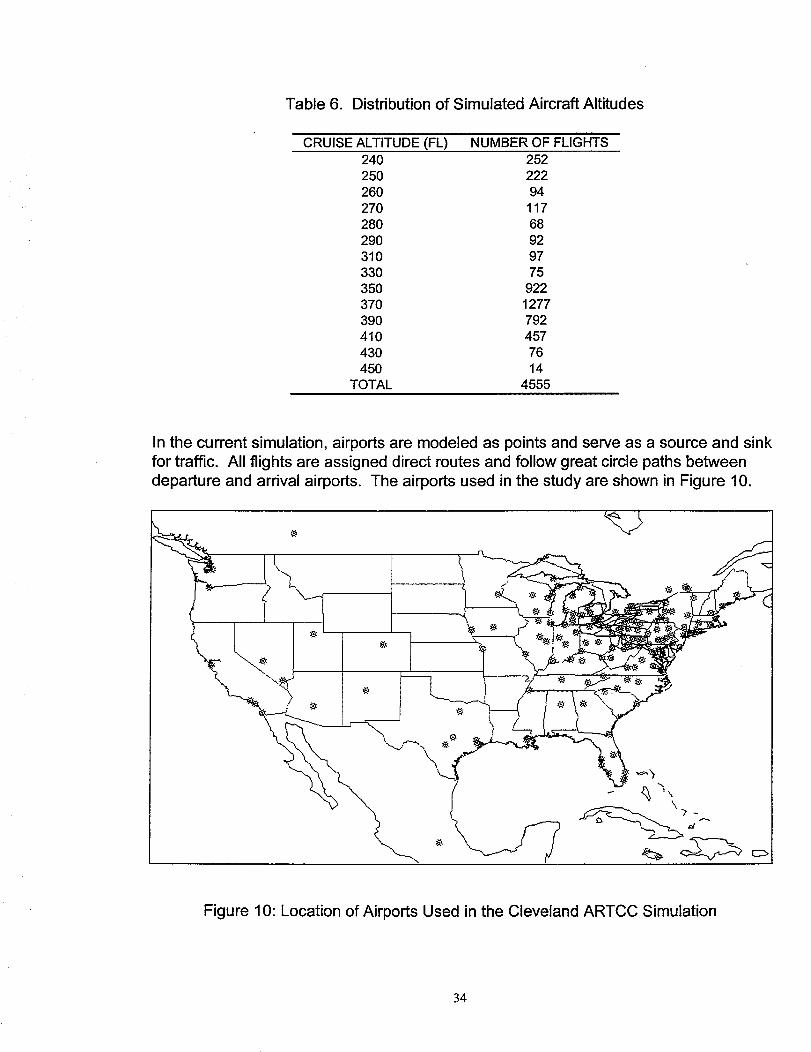
Table 6. Distribution of Simulated Aircraft Altitudes
CRUISE ALTITUDE (FL) NUMBER OF FLIGHTS240 252250 222260 94270 117280 68290 92310 97330 75350 922370 1277390 792410 457430 76450 14
TOTAL 4555
In the current simulation, airports are modeled as points and serve as a source and sink
for traffic. All flights are assigned direct routes and follow great circle paths between
departure and arrival airports. The airports used in the study are shown in Figure 10.
\\
\
Figure 10: Location of Airports Used in the Cleveland ARTCC Simulation
34

Some of the city pair routes used in the study are shown in Figure 11. This figure
shows the density of east/west crossing routes that makes the Cleveland ARTCC anappropriate region to study for free flight. Procedures in and out of the airport,
runways, gates, etc. are not modeled. Further work could include modeling entry andexit points and procedures in and out of a terminal area or airport.
\
\
Figure 11 City Pair Routes Active During Mid-Day Traffic
In our TAAM simulation a full day of traffic is simulated. Aircraft fly undisturbed flightpaths, i.e. conflicts are detected, but not resolved. As the simulation runs, the closest
point of approach (CPA) between each aircraft pair is monitored. If the closest point of
35

approach is between 0%-200% of the separation standard, an encounter is recorded.For each encounter the distance between aircraft at the point of closest approach isrecorded. The encounter data are used to compute the number of ATC interventions
for a given separation requirement. These interventions are a measure of controllerworkload. (In this study the number of encounters which would result in a tactical
intervention is used to quantify center workload. Although many other factors in realitydetermine controller workload, it is here assumed that encounter frequency may be
used as a gross measure of workload for establishing separation requirements.)
Path conflicts are categorized by type of conflict (opposing, in-trail, or crossing) andphase of flight for the pair (descent-descent, climb-climb, cruise-cruise, climb-descent,
climb-cruise, descent-cruise). Aircraft are in-trail if the difference in aircraft heading isless than 45 °, opposing if greater than 135 °, otherwise they are crossing. Aircraft are in
climb mode prior to Top of Climb, in descent mode past Top of Descent. Otherwisethey are assumed to be in cruise mode.
During a simulation, encounters are recorded. Then they are post-processed to remove
encounters that are counted twice. For example, TAAM may count the same encountertwice if the pair of aircraft crosses a sector border while in conflict (counted once ineach sector), or if the duration of an encounter continues to the next hour (counted
once in each hour bin). Also encounters are removed if both aircraft depart from thesame airport since departure procedures are not simulated.
3.1.2 Cleveland ARTCC Simulation Methodology
A total of five operational concepts are considered: the Benchmark system of today'senvironment, Baseline free flight, Baseline plus RVSM, En Route UPT, and En Route
UPT plus RVSM. A listing of studies and their attributes is provided in Table 7.
Table 7. Operational Concepts and Their Attributes
Studies
Attributes
Baseline Free
Flight
User Preferred
Flight Levels
1000 Feet FlightLevels Above
FL290
Unconstrained
Terminal Areas
User Preferred
Routes Between
Terminal Areas
Benchmark NO NO NO NO
NO NO NO YES
NOBaseline Plus
RVSM
NO YES YES
En Route UPT YES NO NO YES
En Route UPT YES YES NO YES
Plus RVSM
36

User Preferred Flight Levels means a flight can use any available flight level. Cruise
altitudes are still assigned by flight levels. We are not considering cruise climbs (i.e.continuous climb during the en route phase of flight). 1000 Feet Flight Levels Above
FL290 means a reduction of the current vertical separation standard above FL290 from
2000 feet to 1000 feet. Unconstrained Terminal Areas means a user is not procedurally
restricted in the terminal area and can fly an optimum departure or approach profile.Optimum approach and departure profiles is desired for free flight, but our simulationmodel needs additional refinement for terminal area studies. Simulation of
unconstrained terminal areas may be considered in future studies. User PreferredRoutes Between Terminal Areas means a user can select a direct route or a minimumwind track outside of the constrained terminal areas. Users also can select their
optimum speed profile.
There are four different TAAM simulations that model the four free flight options. Itshould be noted that the results for the benchmark studies were obtained with the
baseline free flight simulation using 1995 traffic levels. For the benchmark case we
have assumed that the number of encounters with direct point-to-point routes is roughly
equal to the number of encounters with conventional routes. This assumption is basedon results from a previous study that shows both sector loading and number of
proximity events are similar for a conventional route system versus direct routing(Ref. 10). Our studies also do not model winds aloft or adverse weather conditions
which may significantly alter traffic loading patterns.
In the simulation studies we evaluate encounter statistics for 1995 benchmark trafficand for traffic growth from 100% to 200% of the 1995 benchmark. If we assume a
nominal 5% per year growth in traffic, then by 2002, the initial year assumed for FreeFlight implementation, traffic will have grown by 140%, and by 2010 aircraft traffic will
have doubled. Thus, we have chosen to evaluate the operational requirements needed
for initial Free Flight using 140% traffic statistics, and the operational requirements formature Free Flight using 200% traffic statistics. Traffic that are not included are
military, cargo, and general aviation. International traffic flying outside North America
also was not modeled. Their effect will be modeled in future studies. Most general
aviation flights cruise at altitudes below FL240, the lowest altitude used in our study.
Statistically valid results are obtained using several Monte Carlo runs for all data sets.For each run, the departure times in the traffic schedule are varied. Sufficient runs aremade to obtain consistent results.
3.2 Simulation Study Results
In this section the simulation results are presented. Results are shown for the 1995
benchmark study, and four free flight concepts: Baseline free flight, Baseline plus
RVSM, baseline free flight with user preferred flight levels (En Route UPT), andEn Route UPT plus RVSM. The studies show how the number of encounters change
37

as traffic increases and as each free flight environment is introduced. For these studies
an encounter is counted whenever an aircraft pair CPA is less than 10 nm. The data
from these studies are used to drive the operational requirements presented in Section
3.3, and to select preferred concepts for further study.
3.2.1 1995 Benchmark Study (Current NAS System)
This section gives the results from the 1995 benchmark simulation and establishes the
relationships that hold for all studies.
The number of encounters per sector during a one day period are shown in Figure 12.
The encounters are plotted hourly for each of the ten high altitude sectors in the
Cleveland ARTCC (See Figure 9). An examination of the individual sector data shows
considerable variation in the daily distribution of peak period encounters.
Consequently, the total number of encounters over all sectors was used in this study tobenchmark center workload. The number of encounters by hour for all sectors is
illustrated in Figure 13. The morning peak is from 7 AM to 8 AM and the evening peakis from 5 PM to 6 PM.
25
2O
Q(/)
O.15
c
0
c11110
o
EZ
5
5 6
Sector ZOB57 Sector Z(
7 8 9 10 11 12 13 14 15 16 17 18 19 20
Time of Day
21 22 23
Figure 12: Benchmark Encounter Statistics Per Sector Per Hour
38
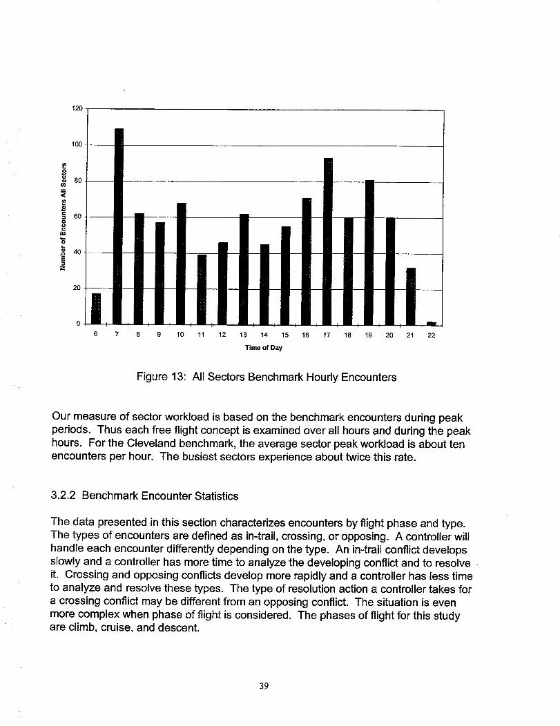
120
100
O
80
c-_ 600
E
Z
2O
6 7 8 9 10 11 12 13 14 15 16 17 18 19 20 21 22
Time of Day
Figure 13: All Sectors Benchmark Hourly Encounters
Our measure of sector workload is based on the benchmark encounters during peak
periods. Thus each free flight concept is examined over all hours and during the peak
hours. For the Cleveland benchmark, the average sector peak workload is about ten
encounters per hour. The busiest sectors experience about twice this rate.
3.2.2 Benchmark Encounter Statistics
The data presented in this section characterizes encounters by flight phase and type.
The types of encounters are defined as in-trail, crossing, or opposing. A controller will
handle each encounter differently depending on the type. An in-trail conflict develops
slowly and a controller has more time to analyze the developing conflict and to resolve
it. Crossing and opposing conflicts develop more rapidly and a controller has less time
to analyze and resolve these types. The type of resolution action a controller takes for
a crossing conflict may be different from an opposing conflict. The situation is even
more complex when phase of flight is considered. The phases of flight for this studyare climb, cruise, and descent.
39

The break down of encounters by type is shown in Table 8.
Table 8. Benchmark Encounters By Type
Morning PeakAll Types 109In-Trail 45
Crossing 34Opposing 29
Evening Peak All Hours93 96744 44820 27429 244
The benchmark encounters by flight phase and type are shown in Table 9.
Table 9. Encounters By Flight Phase and Type - All Hours
AII Types
Climb-Climb
53
Climb-Descent
129
Climb-Cruise307
Cruise-Descent
236
Descent-Descent
74
Cruise-Cruise
166
Total
967In-Trail 14 47 110 104 37 135 448
Crossing 19 44 85 72 22 30 274Opposing 19 38 111 60 14 0 244
The data in these tables are averaged over several Monte Carlo runs to increase the
number of samples and to remove some statistical uncertainties. Runs are varied by
changing the departure times in the simulation schedule. The encounters are totaled for
all sectors. Table 8 shows that the peak period and the all hours encounter data are
consistent, i.e. the in-trail encounters predominate in each case, and the crossing and
opposing encounters are roughly equal in magnitude.
The data in Table 9 further categorizes these encounters by flight phase. The four plots
in Figures 14 to 17 illustrate the data in Table 9. The plots show the phases of flight
that are most prevalent for each type of encounter. In Figure 14 the plot of all types
reveals that encounters mainly involve at least one of the pair being in cruise mode.
The in-trail type of encounter shown in Figure 15 usually involves at least one cruise
aircraft (cruise-cruise, climb-cruise, descent-cruise), whereas crossing and opposing
encounters (Figures 16,17) mainly involve climbing and descending aircraft (climb-
cruise, descent-cruise, climb-descent). It may be noted that there are no cruise-cruise
opposing encounters due to the east-west cruise altitude constraints.
3.2.3 Benchmark Sensitivity Studies
This section presents two benchmark sensitivity studies: the scaling law for close
encounters, and the effect of procedural controls on encounters.
4o

350
0
om
LU
O o
E-
300
250
200
150
100
5O
53
129
307
236
74
dimb-climb climb-descent climb-cruise cruise-descent descent-descent
Phase of Flight
Figure 14: Benchmark Encounters By Flight Phase - All Types
166
cruise-cruise
140 136
o=
o o
=5Z
120
100
80
6O
4O
20 14
climb-climb
Figure 15:
47
110
104
37
climb-descent climb-cruise cruise-descent descent-descent cruise-cruise
Phase of Flight
Benchmark Encounters By Flight Phase - In-Trail Type
41
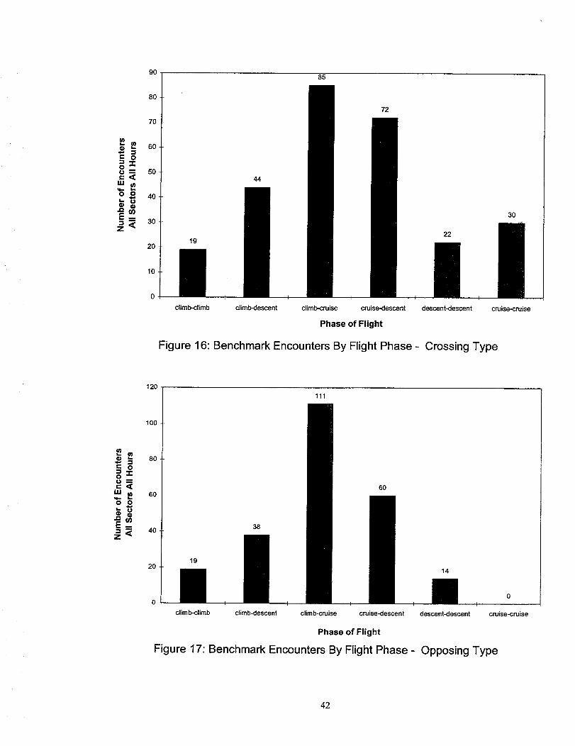
9O85
8O
7O
8_ 50I,LI$,,,
0 0 40
_ 30
2O
10
19
44
72
22
3O
climb-climb climb-descent climb-cruise cruise-descent descent-descent cruise.cruise
Phase of Flight
Figure 16: Benchmark Encounters By Flight Phase - Crossing Type
120
r. 0
5=0 --"
o o
E mm
lO0
80
60
40
2O
111
60
38
19
14
o
climb-climb climb-descent climb-cruise cruise-descent descent-descent cruise-cruise
Phase of Flight
Figure 17: Benchmark Encounters By Flight Phase - Opposing Type
42
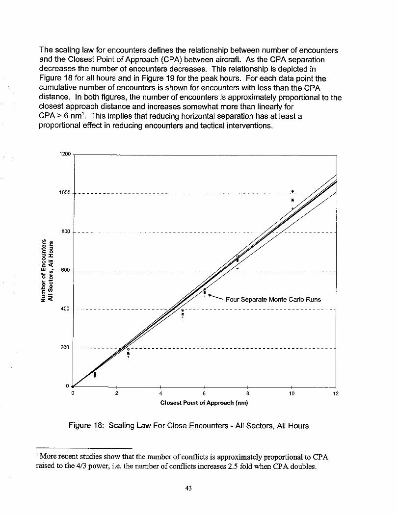
The scaling law for encounters defines the relationship between number of encounters
and the Closest Point of Approach (CPA) between aircraft. As the CPA separation
decreases thenumber of encounters decreases. This relationship is depicted in
Figure 18 for all hours and in Figure 19 for the peak hours. For each data point thecumulative number of encounters is shown for encounters with less than the CPA
distance. In both figures, the number of encounters is approximately proportional to the
closest approach distance and increases somewhat more than linearly for
CPA > 6 nm 1. This implies that reducing horizontal separation has at least a
proportional effect in reducing encounters and tactical interventions.
1200
1000 .................................................... t __ _
C O
"_-rOM
W,_g0 0
e_
80O
600 ................................. +
400
Four Separate Monte Carlo Runs
2OO
0 _ I I
0 2 4 6 8
Closest Point of Approach (rim)
10 12
Figure 18: Scaling Law For Close Encounters - All Sectors, All Hours
1More recent studies show that the number of conflicts is approximately proportional to CPA
raised to the 4/3 power, i.e. the number of conflicts increases 2.5 fold when CPA doubles.
43
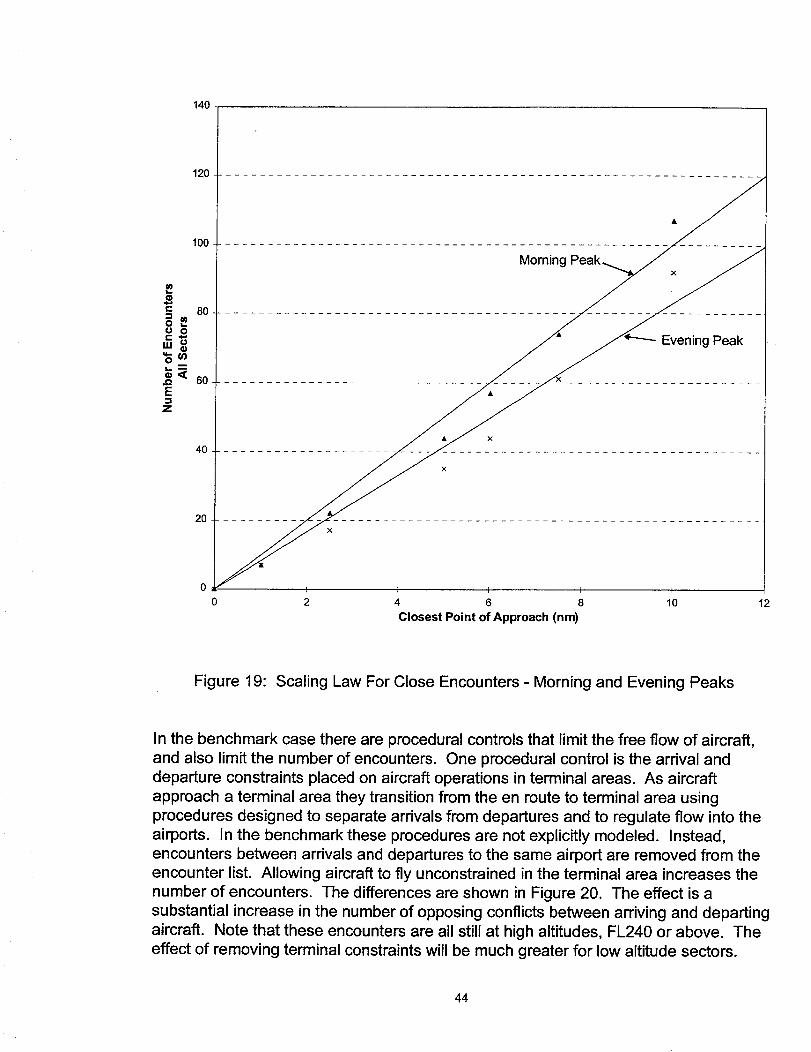
140
120
p,
EZ
100
80
60
4O
Morning
Evening Peak
20 .........
! I t I I
0 2 4 6 8 10
Closest Point of Approach (nm)
12
Figure 19: Scaling Law For Close Encounters - Morning and Evening Peaks
In the benchmark case there are procedural controls that limit the free flow of aircraft,
and also limit the number of encounters. One procedural control is the arrival and
departure constraints placed on aircraft operations in terminal areas. As aircraft
approach a terminal area they transition from the en route to terminal area using
procedures designed to separate arrivals from departures and to regulate flow into the
airports. In the benchmark these procedures are not explicitly modeled. Instead,
encounters between arrivals and departures to the same airport are removed from the
encounter list. Allowing aircraft to fly unconstrained in the terminal area increases the
number of encounters. The differences are shown in Figure 20. The effect is a
substantial increase in the number of opposing conflicts between arriving and departing
aircraft. Note that these encounters are all still at high altitudes, FL240 or above. The
effect of removing terminal constraints will be much greater for low altitude sectors.
44
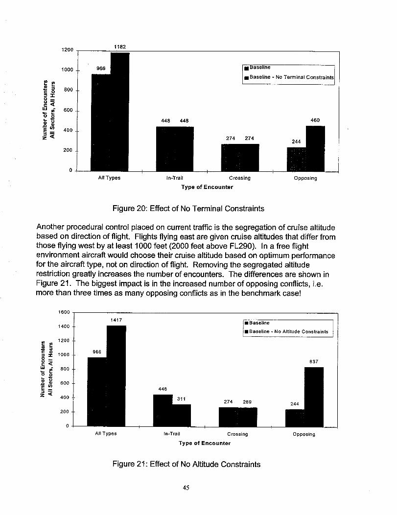
11821200
.=.=
•"_ "ro m
I11
o o
E _-
1000
800
600
400
200
966
[] Baseline Constraints==Base ne - No Terminal
448 448 460
274 274244
--Jc-- H.
All Types In-Trail Crossing Opposing
Type of Encounter
Figure 20: Effect of No Terminal Constraints
Another procedural control placed on current traffic is the segregation of cruise altitude
based on direction of flight. Flights flying east are given cruise altitudes that differ fromthose flying west by at least 1000 feet (2000 feet above FL290). In a free flightenvironment aircraft would choose their cruise altitude based on optimum performance
for the aircraft type, not on direction of flight. Removing the segregated altituderestriction greatly increases the number of encounters. The differences are shown in
Figure 21. The biggest impact is in the increased number of opposing conflicts, i.e.more than three times as many opposing conflicts as in the benchmark case!
1600
E= o= ,-¢o _
u,I
o o
E_
1400
1200
1000
8OO
600
400
2OO
0
966
1417
448
311274 269
All Types In-Trail Crossing
Type of Encounter
• Baseline
• Baseline- No Altitude Constraints ,
837
244
F
Opposing
Figure 21: Effect of No Altitude Constraints
45

These studies illustrate the challenge in moving from procedural, constrained flight toless-constrained free flight concepts. As we remove flight restrictions, we must
simultaneously reduce separation standards and potential conflicts in order to manageencounters, while maintaining or improving current safety margins.
3.2.4 Free Flight Studies - Baseline Concept
Initial free flight operations are expected to begin by the year 2002. It is assumed in
this time period that the surveillance system will be radar based, but incrementallyupgraded for free flight operations. The simulation studies carried out for this reportassume that initial free flight will be constrained to limit the number of encounters andthe controller intervention rate.
The Baseline free flight concept assumes direct routing in the en route phase, butincludes terminal area constraints and en route altitude constraints to reduce aircraftconflicts. Terminal area constraints will reduce the number of conflicts between arrivals
and departures to or from nearby airports. Altitude constraints will reduce the number
of conflicts between opposing traffic in the en route phase of flight. Terminal area
constraints control the flight profile that an aircraft follows to arrive or depart at anairport. They are needed to limit the number of arrival and departure conflicts and also
to allow controllers to set up an efficient arrival stream of traffic. Flight profiles areconstrained by terminal area entry and exit points that are typically located 30 nm or
more from the airport. With the Baseline concept, aircraft can fly direct routes oroptimum wind routes between terminal exit and terminal arrival points.
In our TAAM simulation aircraft fly direct to the airport. Terminal area procedures arenot simulated, but their effect is modeled by removing encounters between arrival and
departures at the same airport. Cruising altitudes are constrained by maintaining asegregated altitude structure between east bound and west bound flights.
Figure 22 shows the increase in encounters as traffic increases from 100% to 200% of
the 1995 benchmark traffic. As traffic increases 40% the number of encounters
increases 86%. The relationship between the number of encounters and traffic load is
nearly quadratic, i.e. doubling the traffic increases the encounters almost four-fold.
Such increases will necessitate major changes in the NAS system to manage theincreased traffic load. The operational requirements to manage such traffic growth isaddressed in Section 3.3.
46
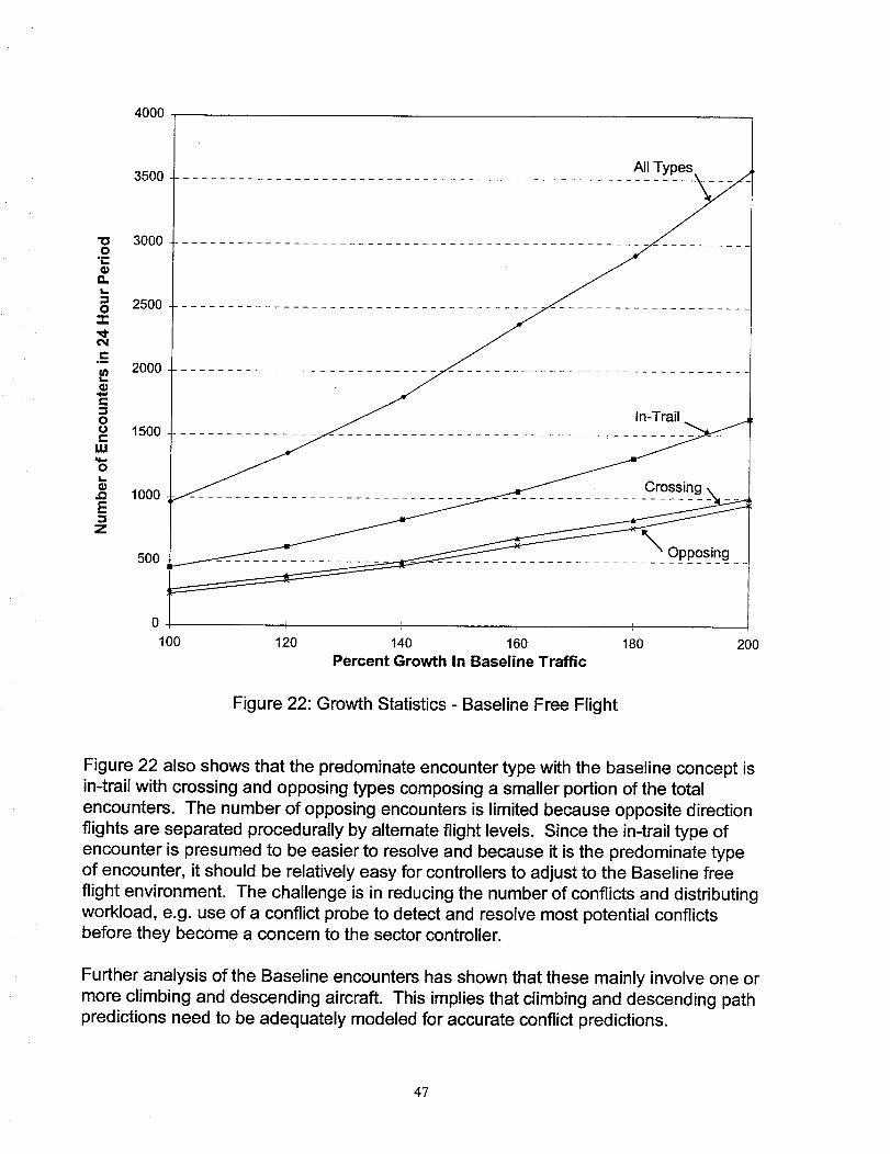
4000
0
230
"I"
e-,m
L.
c
0(3c:
I,Ll
0
E
Z
3500
3000
250O
2000
1500
1000
5OO
100 120 140 160 180 200
Percent Growth In Baseline Traffic
Figure 22: Growth Statistics - Baseline Free Flight
Figure 22 also shows that the predominate encounter type with the baseline concept is
in-trail with crossing and opposing types composing a smaller portion of the total
encounters. The number of opposing encounters is limited because opposite direction
flights are separated procedurally by alternate flight levels. Since the in-trail type of
encounter is presumed to be easier to resolve and because it is the predominate type
of encounter, it should be relatively easy for controllers to adjust to the Baseline free
flight environment. The challenge is in reducing the number of conflicts and distributing
workload, e.g. use of a conflict probe to detect and resolve most potential conflictsbefore they become a concern to the sector controller.
Further analysis of the Baseline encounters has shown that these mainly involve one or
more climbing and descending aircraft. This implies that climbing and descending path
predictions need to be adequately modeled for accurate conflict predictions.
47
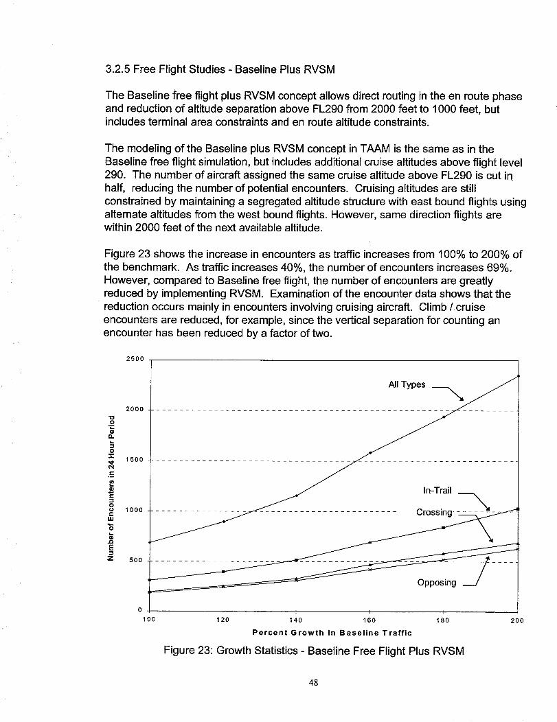
3.2.5 Free Flight Studies - Baseline Plus RVSM
The Baseline free flight plus RVSM concept allows direct routing in the en route phase
and reduction of altitude separation above FL290 from 2000 feet to 1000 feet, butincludes terminal area constraints and en route altitude constraints.
The modeling of the Baseline plus RVSM concept in TAAM is the same as in the
Baseline free flight simulation, but includes additional cruise altitudes above flight level
290. The number of aircraft assigned the same cruise altitude above FL290 is cut in
half, reducing the number of potential encounters. Cruising altitudes are still
constrained by maintaining a segregated altitude structure with east bound flights using
alternate altitudes from the west bound flights. However, same direction flights arewithin 2000 feet of the next available altitude.
Figure 23 shows the increase in encounters as traffic increases from 100% to 200% of
the benchmark. As traffic increases 40%, the number of encounters increases 69%.
However, compared to Baseline free flight, the number of encounters are greatly
reduced by implementing RVSM. Examination of the encounter data shows that the
reduction occurs mainly in encounters involving cruising aircraft. Climb/.cruise
encounters are reduced, for example, since the vertical separation for counting an
encounter has been reduced by a factor of two.
2500
2000
O
Q
1500
Oo 1000cW
0
100
,n-,'ra,........................cross
I I I I
120 140 160 180
Percent Growth In Baseline Traffic
Figure 23: Growth Statistics - Baseline Free Flight Plus RVSM
200
48

One caveat to these results is that the encounter statistics assume perfect knowledge
of the actual aircraft paths. In practice, interventions are based on trajectory predictions
with significant path uncertainty errors. In order to reduce interventions involving
climbing and descending aircraft, it may be necessary to also reduce the vertical path
surveillance errors, i.e. implementing RVSM without reducing path uncertainty isunlikely to yield a significant reduction in interventions. One method to reduce vertical
path uncertainty is to use ADS broadcast of altitude and altitude rate, enhancing the
ability to predict level crossings of potentially conflicting aircraft.
3.2.6 Free Flight Studies - En Route User Preferred Trajectories (UPT)
In this section we examine two mature free flight options where en route altitude
restrictions are removed. The first option is En Route UPT (without RVSM). The
second option is En Route UPT plus RVSM.
The En Route UPT concept allows direct routing in the en route phase and removes the
alternating altitude structure for east and west traffic, but still includes 2000 foot flight
levels above FL290. It also includes terminal area constraints. Removing altitude
constraints increases the number of conflicts between opposing traffic in the en route
phase of flight, but gives the user the benefit of selecting a more fuel optimum altitude.
The implementation of En Route UPT will also require additional infrastructure to
manage the en route opposing conflicts.
The modeling of the En Route UPT concept in TAAM is the same as the Baseline freeflight simulation, but allows east and west traffic to mix at all cruise levels. Aircraft
previously assigned to one altitude are separated evenly between two altitudes with half
of the aircraft remaining at the same altitude and the other half using the next lowest
altitude. The number of aircraft at each en route altitude remains the same, but now
there are aircraft cruising in opposite directions at the same altitude.
Figure 24 shows the increase in encounters as traffic increases from 100% to 200% of
the benchmark. The opposing conflicts dominate this case, with about three times as
many opposing encounters compared to crossing or in-trail encounters. Compared to
the Baseline free flight and Baseline plus RVSM studies, the total number of encounters
has also greatly increased. (See Figure 26).
49

6000
,,_0
._-
nt._
Z30
"I"
r-°l
L_
cD0oc
LIJ
0L_
E
Z
5000
4000
3000
2000
1000
Opposing,_
In-Trail
0 I i i i
100 120 140 160 180
Percent Growth In Baseline Traffic
Crossing
200
Figure 24: Growth Statistics - En Route UPT
Interviewed controllers have indicated that opposing encounters are much harder to
deal with than in-trail encounters, since the time scale for conflict resolution is greatly
compressed. In both the Baseline free flight and Baseline plus RVSM concepts, the
predominate encounter type is the in-trail encounter. The challenge in implementing
the En Route UPT concept is not only to reduce the number of conflicts, but also to
resolve more difficult opposing encounters.
The second mature free flight option is En Route UPT plus RVSM. The user benefitsare the same as En Route UPT. However, the number of aircraft at the same cruise
altitude above FL290 is now cut in half, reducing the number of potential encounters.
The results are shown in Figure 25. The number of encounters is significantly reducedfrom En Route UPT and is even lower than the number of encounters in the Baseline
free flight option. However, en route opposing encounters predominate.
5O

3500
3000
AII Types
"o0
.o-
nl_
0"I"
c_r-
°_
cD0oe.
ILl
0L-
r_E
Z
2500
2000
1500
1000
500
Opposing x,_
In-Trail
0
100 120 140 160 180
Percent Growth In Baseline Traffic200
Figure 25: Growth Statistics - En Route UPT Plus RVSM
3.2.7 Summary
A total of five operational concepts have been considered: the benchmark system of
today's environment, Baseline free flight, Baseline plus RVSM, En Route UPT, and
En Route UPT plus RVSM.
51

For comparison the results of the four free flight options are shown in Figure 26. The
figure shows the growth rate in encounters for the four free flight options. The options
with the highest number of encounters will require the lowest separation minimums to
manage intervention frequency. The relationship between growth in traffic and number
of encounters is nearly quadratic for all four scenarios. The number of encounters for
the benchmark study is the first point of the baseline free flight curve, about 1000
encounters. The operational requirements to implement free flight and still maintain
benchmark encounter levels is explored in the next section.
6000
o.1l_
O.L_
o-l-
e-
ww._
0oe-
ILl
0i_
J2E
Z
5O00
4OOO
3OOO
2OOO
1000
En Route UPT_
Baseline
En Route UPT
Plus
Baseline Plus RVSM
0
100
1995 Benchmark]
i ] I t
120 140 160 180
Percent Growth in Baseline Traffic2OO
Figure 26: Growth Statistics - Four Free Flight Options
52

Table 10 summarizes the expected growth in encounters as traffic grows. Data isshown for all hours. Tables 11 and 12 show the expected growth in encounters for the
morning peak and the evening peak respectively. We will use these tables inSection 3.3.
Table 10. Projected Growth of Encounters - All HoursTraffic Growth Baseline Baseline En Route UPT En Route UPT
Free Flight Plus RVSM Plus RVSM100% 967 685 1418 842
140% 1795 1158 2744 1606
200% 3578 2349 5474 3248
Table 11. Projected Growth of Encounters - Morning PeakTraffic Growth Baseline Baseline .En Route UPT En Route UPT
Free Flight Plus RVSM Plus RVSM100% 109 85 157 98
140% 182 111 22 163
200% 358 226 531 295
Table 12. Projected Growth of Encounters - Evening PeakTraffic Growth Baseline Baseline En Route UPT En Route UPT
Free Flight Plus RVSM Plus RVSM100% 93 61 158 92
140% 176 115 298 169
200% 354 230 596 361
3.3 Operational Requirements and Preferred Free Flight Transitions
The basic idea in this section is to determine system requirements such that the numberof interventions for initial and mature Free Flight operations does not substantially
exceed that for the 1995 benchmark. The assumption here is that the ATC workload inbusy Centers is already maximized for the number of ATC controllers employed, i.e.that controllers are currently workload saturated in the operations they can handle inpeak traffic. This section normalizes the total number of interventions for each Free
Flight concept by applying reduced separation minimums which will limit the growth in
Center operations and intervention frequency to that of the current system.
In the current NAS system, the horizontal separation standard for en route radar control
is 5 nm. However, controllers will typically not intervene when the predicted CPA of an
53

encounter is more than 10 nm, and will intervene when the predicted CPA is less than
10 nm to assure safe separation including path prediction errors such as radar errors
and uncertain;cy in aircraft intent. The effective threshold above which a controller (or
conflict alerting process) will not intervene is very important for Free Flight operations
and is here called the intervention standard, in contrast with the separation standard.
For the benchmark system, all the encounters examined previously would precipitate a
tactical intervention to assure safe separation. One factor which we have ignored in ourstudies is the uncertainty in predicting aircraft altitude, i.e. the number of interventions
could be much larger than the number of encounters, since the altitude buffer for
interventions may be several times that of the vertical separation standard. (Future
simulation studies would explicitly address this issue. See section 5.)
If the number of interventions are to be limited as traffic grows, then the intervention
threshold must shrink to compensate for increased traffic encounters. If we compare
the number of benchmark encounters (section 3.2.2) with the number of interventions
allowed for Baseline operations with 140% traffic growth (section 3.2.7), we find that the
number of interventions needs to be scaled by approximately 1000 / 1800 ~ 56%.
Using the linear scaling law relating number of close encounters to CPA distance, we
see that this is equivalent to reducing the intervention threshold for moving aircraft from
10 nm to about 5.5 nm. However, for current operations we made the simplifyingassumption that all encounters with less than 10 nm CPA would create an ATC
intervention, and all encounters greater than 10 nm would not. Thus, the reduction from
10 to 5.5 nm CPA is for a deterministic threshold based on zero sensor error, whereas
an operational conflict detection system (manual or automated) has an uncertainty banddefining the CPA region where most conflict detections occur.
Below we translate the number of interventions for the four Free Flight transition
concepts into deterministic CPA thresholds, and then select uncertainty bands based on
CNS assumptions to obtain specific separation requirements for the various options.
From the traffic intervention data in the previous section we derive the following values
for the required CPA threshold corresponding to Initial and Mature Free Flight, and for
Baseline, Baseline plus RVSM, En route UPT, and En route UPT plus RVSM:
Table 13. Deterministic CPA Thresholds for Proposed Free Flight Concepts
Baseline Baseline + En route UPT En route UPT
RVSM + RVSM
Initial Free Flight 10* 970 / 1800 10 * 970 / 1160 10 * 970 / 2740 10 * 970 / 1600
(140% Traffic) - 5.5 nm - 8.0 nm - 3.5 nm ~ 6.0 nm
Mature Free Flight 10* 970 / 3580 10 * 970 / 2350 10 * 970 / 5470 10 * 970 / 3250
(200% Traffic) - 2.5 nm - 4.0 nm ~ 1.8 nm - 3.0 nm
54

We now translate the deterministic thresholds into separation assurance parameters.
Figure 27 shows a notional sketch of the assumed detection probability fordeterministic thresholding with no prediction errors, and for an operational conflict
detection process. It is required for an operational system to detect almost all of theconflicts where the CPA is less than the separation standard, and to declare conflicts onat most a few percentage of the encounters where the CPA exceeds the intervention
standard, i.e. unnecessary alerts or false alarms. As a first approximation, we assume
that the detection probability falls off linearly as CPA increases from the separationstandard to the intervention standard, as shown in Figure 27. Then the total number ofinterventions for an operational system is approximately the same as that with a
deterministic threshold placed at the midpoint of the CPA uncertainty region, i.e. thedeterministic threshold is approximately equal to the average of the separation standardand the intervention standard.
For the Baseline flight option with an implementation date of 2002, we can allow an
uncertainty band of 3.5 nm for the CPA uncertainty region, assuming fusion of Radarand Flight Plan data for path predictions. Using a deterministic threshold of 5.5 nm from
Table 13 and placing this threshold near the center of the CPA uncertainty region yieldsa separation standard of 4 nm and an intervention threshold of 7.5 nm. In other words,if almost all of the encounters with CPA less than 4 nm are detected, and all but a few
percent of the encounters with CPA greater than 7.5 nm are not, then the total numberof interventions is roughly equivalent to a deterministic threshold of about 5.5 nm. in
this case the separation standard reduces from 5 nm with the current system to 4 nmwith Initial Free Flight, and the uncertainty band for conflict decisions shrinks from 5 nmto 3.5 nm.
Probability ofDetection
......................................................... Deterministic
S CPA Thresh°ld
_i /- C°ten_cfiCtn
. _ Process
Separation i _ Intervention
Closest Approach Distance (CPA)
Figure 27: Sketch of Conflict Detection Thresholding Values
55
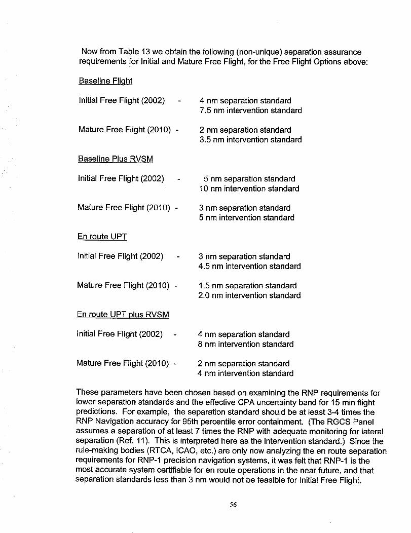
Now from Table 13 we obtain the following (non-unique) separation assurance
requirements for Initial and Mature Free Flight, for the Free Flight Options above:
Baseline Fliqht
Initial Free Flight (2002) 4 nm separation standard7.5 nm intervention standard
Mature Free Flight (2010) 2 nm separation standard3.5 nm intervention standard
Baseline Plus RVSM
Initial Free Flight (2002) 5 nm separation standard10 nm intervention standard
Mature Free Flight (2010) - 3 nm separation standard5 nm intervention standard
En route UPT
Initial Free Flight (2002) 3 nm separation standard4.5 nm intervention standard
Mature Free Flight (2010) 1.5 nm separation standard2.0 nm intervention standard
En route UPT plus RVSM
Initial Free Flight (2002) 4 nm separation standard8 nm intervention standard
Mature Free Flight (2010) - 2 nm separation standard4 nm intervention standard
These parameters have been chosen based on examining the RNP requirements for
lower separation standards and the effective CPA uncertainty band for 15 min flightpredictions. For example, the separation standard should be at least 3-4 times the
RNP Navigation accuracy for 95th percentile error containment. (The RGCS Panel
assumes a separation of at least 7 times the RNP with adequate monitoring for lateralseparation (Ref. 11). This is interpreted here as the intervention standard.) Since therule-making bodies (RTCA, ICAO, etc.) are only now analyzing the en route separationrequirements for RNP-1 precision navigation systems, it was felt that RNP-1 is the
most accurate system certifiable for en route operations in the near future, and that
separation standards less than 3 nm would not be feasible for Initial Free Flight.
56

We now consider which of these options are preferred for further analysis. For the
Initial Free Flight implementation, the Baseline option is preferred compared to the other
options in terms of needed infrastructure. This is because the Baseline option can beimplemented using existing radar technology for surveillance, whereas we will need
data-link and some form of ADS reporting for implementing the other options. (Inparticular, the conflict probe studies in the next section will show that with radar
improvements we can reasonably expect to obtain CPA uncertainty bounds on the
order of 3 - 4 nm, but to obtain uncertainty bounds on the order of 2 nm or less andsatisfy reasonable Iookahead constraints will require more accurate ADS based
surveillance.) The Baseline option will require precision navigation (RNP-1) in order toaccommodate opposing traffic conflicts, and will require substantial improvements to theradar tracking system, and implementation of several Center automation functions inorder to accommodate a 4 nm separation standard and shrink the intervention standard
to 7.5 nm. However, there is not a high risk in implementing these improvements since
all the basic technologies are currently in place. Consequently, we have selected theBaseline flight concept with the above horizontal separation parameters for the InitialFree Flight transition.
The preferred Free Flight concept may change significantly, however as we movetowards mature Free Flight, and traffic growth necessitates further reduction in
separation standards. In order to implement a 2 nm separation standard and 3.5 nm
intervention standard for the Baseline Free Flight concept, significant changes in boththe surveillance system and in resolution of conflicts would be needed. The most
significant changes are the addition of ADS surveillance to reduce the uncertainty inCPA geometry, and the implementation of an Alert Zone concept and associated Free
Flight path restrictions. The problem with the Baseline concept for mature Free Flight isthat even with significant changes in onboard avionics and onboard situation
awareness, cruise altitudes remain limited to 4000 foot discrete steps above FL290.Consequently, it makes sense to implement RVSM when the transition to ADS occurs,
as a system-wide infrastructure upgrade. Alternately, one can transition from theBaseline Free Flight system to an En route UPT system with no cruise restrictions and
with a simultaneous transition to ADS surveillance and Alert Zone path restrictions.
The preferred next step to Free Flight is the Baseline Plus RVSM concept, since it hasthe greatest economic value for users, with the least reduction in separation parametersto accommodate future traffic growth. By contrast the Baseline and En route UPT Free
Flight concepts will either require more costly infrastructure or will have less safetymargin since their separation parameters are significantly smaller. However, theBaseline plus RVSM concept requires that all airspace users flying at or above
FL2.90, including those not flying Free Flight paths, be equipped for RVSM. If this FreeFlight option is considered too restrictive in scope, then the alternative En route UPT
option may be preferred as the next step toward Free Flight.
5"7

The transitionto Mature Free Flight is completed using the En route UPT plus RVSM
concept, which again requires reduced separation standards compared with theBaseline plus RVSM concept. However, the horizontal separation standards are much
less severe than those for the En route UPT concept without RVSM. (In fact the 1.5 nm/ 2.0 nm separation parameters for Mature Free Flight are probably unrealistic
requirements for automated conflict detection with a 15 minute Iookahead period.)Consequently, the above transition path to Mature Free Flight was selected as the basisfor the operational requirements in this study.
The operational requirements for separation assurance with the preferred Free Flighttransition concepts are summarized in Table 14. The Initial Free Flight implementationis the Baseline concept with a target date of 2002. The primary infrastructure
requirement onboard is an RNP-1 navigation system. Considerable ground-basedinfrastructure is needed in the Centers, however, to support the medium term conflict
probe and the Radar controller in attaining the reduced separation parameters shown.This transitional system would be replaced sometime later in the decade with a jointradar / ADS surveillance system permitting a further reduction in both horizontal and
vertical separation standards. This would require more extensive changes to theaircraft avionics and to flight procedures to safely implement the reduced separations.Even those aircraft flying current routes and procedures would need modifications for
compatibility with this system, i.e. increased altitude precision and ADS capability maybe required for all aircraft flying in high altitude airspace with this transition path. The
final transition to En route UPT plus RVSM, where same altitude opposing conflicts maybe routinely encountered, will require significant prior development and experiencegained in implementing the previous steps.
The separation and intervention standards shown in Table 14 do not take into
consideration the effect of wake turbulence as two aircraft approach within severalnautical miles during a close encounter. Considerable research is needed to betterunderstand the effect of wake turbulence on en route encounters and to establish the
limits imposed on separation standards by the physics of such encounters. The
conclusions of this section are thus preliminary, and need to be validated or modifiedbased on research in this area.
58

Table 14. Selected Separation Parameters and Transition to Mature Free Flight
SeparationStandard
* 5 nm- Radar
* 4 nm- Radar
* 3 nm - Radar /
ADS Monitor
+
1000 fl RVSM
* 2 nm - Radar
/ADS Monitor
+
1000 ft RVSM
InterventionStandard 1
* 10 nm- Manual
* 7.5 nm- Manual
+ Automation Tools
* 5 nm - Manual +
Semi-Automated
Conflict Resolution
* 4 nm- Manual
+
Semi-Automated
Conflict Resolution
IOCDate
*Today
* 2002
* 2006
* 2010
Ops Concept &Infrastructure
NAS ATC System
* - 10 sec Radar Monitor
Baseline Free Flight
* RNP-1 Navigation
* Improved Tracking
* Improved Wind Forecasts
* 10-20 min Conflict Probe
*Future Intent Display Aids
Baseline Plus RVSM
* Above Plus
RVSM Sensor
ADS Reporting
Radar/ADS/FP Fusion
En route UPT Plus RVSM
* Above Plus
- RNP 0.5 Navigation
- High Integrity
Cooperative Separation
- Alert Zone Restrictions
1Thresholds for In-Trail & Crossing Trajectories ( May be Different for Opposing )
It should be noted that the conclusions and operational requirements derived from theTAAM simulation model are tentative, i.e. substantial validation of the TAAM model isrequired before these results can be considered definitive. In section 5 we discuss
follow-on tasks which are recommended for improving and validating the TAAM modelfor Free Flight studies. These tasks address the issue of validation of aircraft
trajectories and airspace density using real-time ETMS data tapes, and validating theTAAM database on airplane performance. The value of the studies to date is that they
give some insight into the challenges inherent in implementing Free Flight.
59
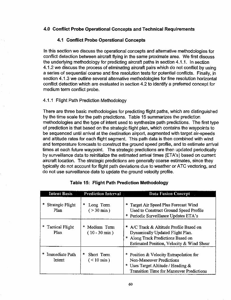
4.0 Conflict Probe Operational Concepts and Technical Requirements
4.1 Conflict Probe Operational Concepts
In this section we discuss the operational concepts and alternative methodologies for
conflict detection between aircraft flying in the same proximate area. We first discuss
the underlying methodology for predicting aircraft paths in section 4.1.1. In section
4.1.2 we discuss the process of eliminating aircraft pairs which do not conflict by using
a series of sequential coarse and fine resolution tests for potential conflicts. Finally, in
section 4.1.3 we outline several alternative methodologies for fine resolution horizontal
conflict detection which are evaluated in section 4.2 to identify a preferred concept for
medium term conflict probe.
4.1.1 Flight Path Prediction Methodology
There are three basic methodologies for predicting flight paths, which are distinguished
by the time scale for the path predictions. Table 15 summarizes the prediction
methodologies and the type of intent used to synthesize path predictions. The first type
of prediction is that based on the strategic flight plan, which contains the waypoints tobe sequenced until arrival at the destination airport, augmented with target air-speeds
and altitude rates for each flight segment. This path data is then combined with wind
and temperature forecasts to construct the ground speed profile, and to estimate arrival
times at each future waypoint. The strategic predictions are then updated periodically
by surveillance data to reinitialize the estimated arrival times (ETA's) based on current
aircraft location. The strategic predictions are generally coarse estimates, since they
typically do not account for flight path deviations due to weather or ATC vectoring, and
do not use surveillance data to update the ground velocity profile.
Table 15: Flight Path Prediction Methodology
Intent Basis Prediction Interval Data Fusion Conce _t
Strategic FlightPlan
Tactical FlightPlan
Immediate Path
Intent
Long Term
(>30min)
Medium Term
( 10 - 30 min )
Short Term
(< 10 min)
* Target Air Speed Plus Forecast Wind
Used to Construct Ground Speed Profile
* Periodic Surveillance Updates ETA's
* A/C Track & Altitude Profile Based on
Dynamically Updated Flight Plan.
* Along Track Predictions Based on
Estimated Position, Velocity & Wind Shear
* Position & Velocity Extrapolation for
Non-Maneuver Predictions
* Uses Target Altitude / Heading &
Transition Time for Maneuver Predictions
6O

Tactical flight path predictions are based on similar intent information as for strategicflight plans, but intent will be updated either by use of ADS air-ground data-link or by aCenter controller when a flight plan change is negotiated. The along track predictions
are based on extrapolating estimated aircraft position and velocity states, and usingalong track wind shear for straight line, constant flight path segments. The
methodology for predicting turn segments and vertical transitions is not explicitly
discussed in this report but could be based on empirical look-up tables (Ref. 13), onassumed guidance laws during the transition phases (similar to CTAS, Ref. 14), or on
ADS down-link of FMS based 4-D waypoints. Whatever method is ultimately used forsuch transitions, relatively high accuracy and ability to estimate prediction error growthare essential elements for medium term conflict detection. (In chapter 5 we comment
further on needed research in this area, since the great majority of aircraft conflictsinvolve non-level flight encounters.) The use of strategic prediction methods formedium term path predictions is not recommended, since aircraft often do not follow
their strategic flight plan, i.e. flight parameters such as cruise altitude, air-speed, andvertical rates may be quite different than those inferred from the flight plan or from
system provided default values. (As an example, the rms error in predicting FIR-exitETA's for overflying flights in an existing, operational system (Ref. 13) is on the order offive times larger than results obtained for the Baseline conflict probe, which assumes
more accurate path prediction methodologies.) Moreover, accurate predictions mayrequire sophisticated flight tracking and conformance monitoring to validate theparameters and guidance laws assumed for the current flight segment.
Short term path predictions typically do not use wind forecasts or flight plan data, andare based on simple extrapolation of the current velocity vector over the forecast
period. However, experience with both the Conflict Alert algorithm used in the ATCCenters and TCAS shows the importance of including short term intent (especially
target altitude) for modifying path forecasts based on intent. This type of informationmay be broadcast in an ADS-B event report in future systems, i.e. prior to and at thestart of a flight transition. Otherwise, such intent data must be input to the prediction
system by a controller or by lookup from the current flight plan. Short term predictionsare usually faidy simple and have limited accuracy due to limitations in the surveillance
system, i.e. large lags and noise errors in estimating velocity vector and altitude rate.Consequently, Iookahead time for Conflict Alert is typically limited to a few minutes, anddoes not exceed 3.5 minutes with current technology radar surveillance (Ref. 15).
The accuracy of medium term path predictions using the above methodology changes
dynamically and has different error mechanisms for lateral, vertical, and longitudinalaxes. In the lateral axis, the primary error sources are navigation and Flight Technical
Error (FTE), since the lateral prediction is based on the tactical flight plan. For an RNP-1 navigation system, the total rms lateral errors should not exceed 0.5 nm, independentof prediction time, although larger lateral errors may be assumed during turn
maneuvers. Although we do not explicitly model vertical predictions in this report, thecovariance methodology discussed below may be appropriate for climb and descent
transitions, and a single rms parameter may be applicable for cruise and level flight
61

segments. In the longitudinal direction, the rms prediction errors grow rapidly withprediction time, reflecting uncertainty in estimating path velocity due to surveillance and
wind forecast errors. In addition, the path length during turning maneuvers is uncertain,
which adds to uncertainty in the longitudinal axis following such maneuvers. Figure 28
illustrates the covariance methodology for modeling horizontal prediction errors as a
time varying ellipse with major axis typically along the longitudinal axis, and minor axis
along the lateral axis. For two proximate aircraft, the size and shape of such error
ellipses at the time of closest approach are vital elements in predicting assured
separation or detecting potential conflicts in a probe Iookahead period.
As an example, suppose we are predicting the one sigma error ellipse for an RNP-1
aircraft with surveillance rms errors = 5 knots, i.e. using the CNS requirements specified
in section 1.5. Then the lateral axis rms is 0.5 nm, and the longitudinal rms error grows
at the rate of 0.5 nm per 6 minute prediction period. Thus the rms longitudinal error
roughly equals the lateral error at T = 6 minutes Iookahead, is about twice the lateral
error at T= 12 minutes, and is about three times the lateral error at T= 18 minutes. This
rapid growth in error uncertainty has important consequences for conflict alerting and
use of the conflict probe in an operational setting. Using similar logic, we find that the
short term prediction method for Conflict Alert has smaller lateral error uncertainty than
the medium term Conflict Probe for Iookahead periods less than 6 minutes, in this
example. Thus the medium term prediction method should only be used for Iookahead
times greater than that for short term Conflict Alert, i.e. we recommend complementary
use of both short term and medium term conflict alerting.
O
L . Intruder Path
-4 _ .J Prediction &Uncertainty
Intruder A/C
At Current Time
Uncertainty Ellipses
At Closest Approach
Reference A/C
_& Position Error
At Current Time/,_.._J,,,,
o i - _ Path UncertaintyAt T= 6 min
Figure 28 : Aircraft Crossing Path Horizontal Geometry (Covadance Modeling)
62

4.1.2 Conflict Detection Automation Process
Figure 29 illustrates the process used to detect conflicts for the probe operational
concept described in section 2.1.2. At each conflict probe update time, or as needed
for trial flight planning, the predicted flight plan of a reference aircraft is subjected to
conflict processing to validate flight plan separation with other aircraft, or to identify and
alert the controller to potential conflicts. The first step is to use a coarse conflict filter to
identify potential intruder aircraft and time segments where the intruder path is near the
reference aircraft during a Iookahead period. These potential intruders are then
subjected to finer resolution tests to declare potential conflicts and to eliminate safely
separated aircraft from further probe testing on later probe updates. For newly
identified aircraft pairs, the probe tests at regular intervals, e.g. one minute updates,
until either a no-conflict or a conflict alert is declared for the aircraft pair. The probe
then inhibits further testing on this pair until either a time-out (nominally = 5 min) is
exceeded, or one of the aircraft is declared out of conformance with its intended flight
plan. Thus, a conflict / no-conflict declaration typically remains in effect for some time
period, and then the aircraft pair is again subject to conflict processing.
Reference
Aircraft Path
Controller
Interface
Coarse
Conflict
Filter
I Path 1Intent
Database
CONFLICT
ALERT
Potential
Intruder
Paths
IProbe
' Inhibit
Logic
( Declare No Conflict )
Vertical
Separation
?
YES
NO MAYBE
NO
Coarse
Horizontal
Separation ?
1NoSeparation
Near Closest
Approach ?
MAYBE _ _ NO
NO [ Separate Horizontal &II
(Declare Conflict) I Vertical Conflict Intervals ?
YES
Figure 29 • Aircraft Pair Filtering and Conflict Detection Process
63
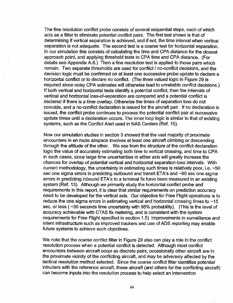
The fine resolution conflict probe consists of several sequential steps, each of which
acts as a filter to eliminate potential conflict pairs. The first test shown is that ofdetermining if vertical separation is achieved, and if not, the time interval when vertical
separation is not adequate. The second test is a coarse test for horizontal separation.In our simulation this consists of calculating the time and CPA distance for the closest
approach point, and applying threshold tests to CPA time and CPA distance. (Fordetails see Appendix A.6.) Then a fine resolution test is applied to those pairs whichremain. Two separate thresholds are used for conflict / no-conflict decisions, and the
decision logic must be confirmed on at least one successive probe update to declare a
horizontal conflict or to declare no conflict. (The three valued logic in Figure 29 is
required since noisy CPA estimates will otherwise lead to unreliable conflict decisions.)If both vertical and horizontal tests identify a potential conflict, then the intervals ofvertical and horizontal loss-of-separation are compared and a potential conflict is
declared if there is a time overlap. Otherwise the times of separation loss do notcoincide, and a no-conflict declaration is issued for the aircraft pair. If no declaration is
issued, the conflict probe continues to process the potential conflict pair at successiveupdate times until a declaration occurs. The inner loop logic is similar to that of existingsystems, such as the Conflict Alert used in NAS Centers (Ref. 15).
Now our simulation studies in section 3 showed that the vast majority of proximate
encounters in en route airspace involves at least one aircraft climbing or descendingthrough the altitude of the other. We see from the structure of the conflict declaration
logic the value of accurately estimating both time to vertical crossing, and time to CPAin such cases, since large time uncertainties in either axis will greatly increase thechances for overlap of potential vertical and horizontal separation-loss intervals. With
current methodology, the uncertainty in estimating such times is relatively poor, i.e. -50
sec one sigma errors in predicting outbound and transit ETA's and ~90 sec one sigmaerrors in predicting inbound ETA's to a terminal fix have been measured in an existing
system (Ref. 13). Although we primarily study the horizontal conflict probe andrequirements in this report, it is clear that similar requirements on prediction accuracyneed to be developed for the vertical axis. Our objective for Free Flight operations is toreduce the one sigma errors in estimating vertical and horizontal crossing times to ~15
sec. or less ( ~30 seconds time uncertainty with 95% probability). (This is the level of
accuracy achievable with CTAS fix metering, and is consistent with the systemrequirements for Free Flight specified in section 1.5) Improvements in surveillance and
intent infrastructure such as improved trackers and use of ADS reporting may enablefuture systems to achieve such objectives.
We note that the coarse conflict filter in Figure 29 also can play a role in the conflictresolution process when a potential conflict is detected. Although most conflictencounters between aircraft occur as discrete pairs, occasionally other aircraft are in
the proximate vicinity of the conflicting aircraft, and may be adversely affected by thetactical resolution method selected. Since the coarse conflict filter identifies potential
intruders with the reference aircraft, these aircraft (and others for the conflicting aircraft)can become inputs into the resolution process to help select an intervention
64
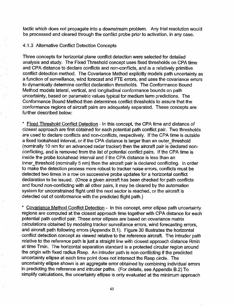
tactic which does not propagate into a downstream problem. Any trial resolution wouldbe processed and cleared through the conflict probe prior to activation, in any case.
4.1.3 Alternative Conflict Detection Concepts
Three concepts for horizontal plane conflict detection were selected for detailed
analysis and study. The Fixed Threshold concept uses fixed thresholds on CPA timeand CPA distance to declare conflicts and non-conflicts, and is a relatively primitive
conflict detection method. The Covariance Method explicitly models path uncertainty asa function of surveillance, wind forecast and FTE errors, and uses the covariance errors
to dynamically determine conflict declaration thresholds. The Conformance Bound
Method models lateral, vertical, and longitudinal conformance bounds on pathuncertainty, based on parametric values typical for medium term predictions. TheConformance Bound Method then determines conflict thresholds to assure that the
conformance regions of aircraft pairs are adequately separated. These concepts arefurther described below:
* Fixed Threshold Conflict Detection - In this concept, the CPA time and distance ofclosest approach are first obtained for each potential path conflict pair. Two thresholds
are used to declare conflicts and non-conflicts, respectively. If the CPA time is outsidea fixed Iookahead interval, or if the CPA distance is larger than an outer_threshold
(nominally 10 nm for an advanced radar tracker) then the aircraft pair is declared non-conflicting, and is removed from the list of potential conflict pairs. If the CPA time isinside the probe Iookahead interval and if the CPA distance is less than an
inner_threshold (nominally 5 nm) then the aircraft pair is declared conflicting. In orderto make the detection process more robust to tracker noise errors, conflicts must be
detected two times in a row on successive probe updates for a horizontal conflictdeclaration to be issued. (Once a given aircraft has been checked for path conflicts
and found non-conflicting with all other pairs, it may be cleared by the automationsystem for unconstrained flight until the next sector is reached, or the aircraft is
detected out of conformance with the predicted flight path.)
* Covariance Method Conflict Detection - In this concept, error ellipse path uncertainty
regions are computed at the closest approach time together with CPA distance for eachpotential path conflict pair. These error ellipses are based on covariance matrix
calculations obtained by modeling tracker surveillance errors, wind forecasting errors,and aircraft path following errors (Appendix B.1 ). Figure 30 illustrates the horizontal
conflict detection concept as viewed relative to the reference aircraft. The intruder pathrelative to the reference path is just a straight line with closest approach distance Rminat time Tmin. The horizontal separation standard is a protected circular region around
the origin with fixed radius Rsep. An intruder path is non-conflicting if the predicteduncertainty ellipse at each time point does not intersect the Rsep circle. The
uncertainty ellipse shown is an aggregate error obtained by combining individual errorsin predicting the reference and intruder paths. (For details, see Appendix B.2) To
simplify calculations, the uncertainty ellipse is only evaluated at the minimum approach
65

time Tmin. The closest approach is then found by sliding the 'frozen' ellipse along theintruder path, generating the dotted line in Figure 30. The uncertainty error Runc canbe determined analytically as the maximum distance of the ellipse from the intruder
path. If Rmin < Rsep + Runc, then a potential conflict exists. In this case, the initial
time (final time) of the conflict is found by sliding the ellipse backward (forward) in timeuntil the circle and ellipse just touch. The methodology for covariance based conflictdetection is summarized in Appendix B.
Current
S Intruder
I "No Conflict" : 1 *_ Position
Rmin>Rsep+Runc) __ S
Reference "',, / "_x \
Path ",_,'_ ]
(At Origin) _'_
Horizontal \ Rsep] ",_ 7\
Separation /__ "_Runc_
Region _
Uncertainty
Ellipse
At Tmin
Ownship
Ground Track
Intruder Path
Figure 30: Covariance Method Conflict Detection Concept
In practice, two error ellipses are used for conflict decisions. The main difference
between declaring conflicts and non-conflicts is in the size of the uncertainty ellipsesused. The error ellipse used to declare non-conflicts is relatively large, on the order oftwo to three times the one sigma prediction errors, in order to reduce the missed detect
probability to an acceptable level. The outer threshold for eliminating non-conflictingpairs is the sum of Rsep and Runc for the large error ellipse. Similarly, the error ellipseused to declare conflicts is relatively small, typically less than one sigma, in order toavoid excessive false alerts resulting in unnecessary tactical interventions. The inner
threshold for identifying potential conflicts is the sum of Rsep and Runc for the smallerror ellipse. The thresholds with this method are dynamic and depend on the
geometry of the conflict and the time to closest approach. The detection logic fordeclaring conflicts and non-conflicts is similar to that with Fixed Thresholds, once the
inner and outer thresholds are computed.
* Conformance Bound Conflict Detection - This concept is a generic version of the
conflict detection method proposed for the AERA-2 program ( Ref. 2, 3). As originally
66

proposed, each Center maintains a strategic, 4-D flight plan for all aircraft entering into
Center controlled airspace. This flight plan reflects the current aircraft intent and is kept
updated by path conformance monitoring and surveillance based flight plan
reconformance if the actual position drifts too far from the predicted flight plan. Conflict
detection with this concept is performed periodically on each aircraft between entry andexit from Center airspace, and whenever aircraft paths are out of conformance with the
intended plan. Fixed size error ellipses are used to model horizontal conformance
bounds for level flight path following (nominally, 1 nm lateral semi-axis by 2 nm
longitudinal semi-axis for conflict declarations). These conformance regions are
expanded during vertical transitions and turn maneuvers. Figure 31 illustrates
horizontal conflict detection with this method. As in figure 30, the intruder path and
location at minimum approach are shown relative to the reference aircraft (ownship).
The conformance bounds for both ownship and intruder paths are represented here as
ellipses centered on the predicted aircraft paths. The conformance ellipses are
obtained by rotating from standard NED coordinates to ownship coordinates with x-axis
along the ownship track. The intruder is considered conflicting if the minimum approach
distance between the conformance bounds becomes less than the separation standard
Rs, as the intruder transits the minimum approach point. This is easily determined byanalytic calculations to calculate the maximum lateral extent of each conformance
ellipse (R1 and R2) in the direction of the minimum approach point. If Rmin < R1 + R2
+ Rs then the aircraft pair are potentially conflicting, i.e. an inner threshold is obtained
by summing R1, R2, and Rs. The detection logic for declaring non-conflicts is similar to
that above, with the outer thresholds for declaring non-conflicts based on larger sizeconformance ellipses, nominally 1.6 times the size of the inner bounds.
Predicted Intruder
Path
Intruder
Cortformance Bound
At Cpa Time
Intruder Positionpa....
. • ......
Ownship _ "'".... .......... \
Conformance Bound __..__"....
Ownship Posi_ 1Rs No Conflict: Rmin > R1 + Rs + R2
(At Origin) ( Rs = Separation Standard )
Figure 31: Conformance Bound Conflict Detection Concept
67
The conformance method is inherently more conservative in declaring conflicts than the
covariance method. This is partly due to the covariance method using dynamicallyupdated bounds on relative prediction error whereas the conformance method uses
a-priori uncertainty bounds, and partly due to maintaining separation between two
conformance bounds rather than using an aggregate bound on prediction errors.
4.2 Baseline Comparisons of Alternative Probe Concepts
In this section we compare the conflict detection performance of the alternative probeconcepts identified in section 4.1. Rather than using surveillance and predictionassumptions relevant for today's ATC system, we here assume conditions relevant to
the Baseline Free Flight concept, i.e. with enhanced radar tracking and enhanced
weather forecasting assumed available in the ATC Centers by 2002. (In section 4.3we show the effect of using coarse tracking and weather forecasting assumptions onprobe performance.) The navigation systems for simulated aircraft encounters also
assume low navigation errors and FTE path following errors, consistent with RNP-1quality airborne avionics. These assumptions are based on the operationalrequirements for initial Free Flight developed in section 3.3. Encounters between
aircraft with lower quality avionics can also be simulated, but the separation andintervention standards would be larger with such encounters.
The modeling assumptions and methodology for evaluating the alternative probeconcepts are first described in section 4.2.1. Section 4.2.2 then presents comparisonsof important performance measures such as missed detections, false alarms, andconflict warning time, and shows the expected number of probe-based conflictinterventions relative to benchmark results for the Cleveland Center simulation. Section
4.2.3 recommends a preferred concept for further study and sensitivity analysis, andsummarizes the performance characteristics of the preferred concept.
4.2.1 Baseline Assumptions and Conflict Probe Performance Analysis
The conflict probe studies are based on Monte-Carlo simulation of horizontal
encounters between aircraft pairs. Figure 32 shows the geometry of a single encounterbetween two aircraft denoted the "ownship" and "intruder". For each trial, the nominal
encounter geometry is fixed and the initial entry conditions are chosen such that adirect collision results if both aircraft fly their flight plan with no FTE errors, and with norandom wind errors. A wind field is generated for each trial, based on a fixed mean
wind with exponentially correlated random wind errors (Ref. 16). In effect, the random
wind errors perturb the along-track velocity vectors of the aircraft at the initial entrytimes, and create along-track wind shear which changes the ground speed of the
aircraft as they move toward the crossing fix. In addition, aircraft navigation and FTEerrors are modeled as a constant lateral offset chosen randomly from trial to trial. Theresult of the random wind field and the lateral offset errors is a close encounter rather
than a direct collision, as the aircraft transit the crossing fix. (Our covariance model can
68

also include longitudinal FTE error modeling, but these errors are ignored in our
studies, since wind and surveillance velocity errors will typically dominate such errors
even with assumed technology enhancements for 2002 operations.)
For each Monte-Carlo study, the mean time for the aircraft to reach the crossing fix is25 min. (This assures that the simulation time exceeds the max Iookahead time for the
conflict probe.) Three different crossing angles are evaluated in our studies: 30 deg
crossing (intrail conflict), 90 deg crossing (crossing conflict), and 150 deg crossing(opposing conflict). The rms error in lateral offset for each aircraft is 0.5 nm, i.e. on
each trial the ownship and intruder are offset laterally from the nominal flight path by arandom distance with mean zero and standard deviation = 0.5 nm. Random winds
were simulated in our studies with mean value = 40 knots, random along-track rmserror = 25 knots, and correlation distance = 670 nm for cross-correlation between winds
at different locations. (The along-track wind shear is about 10 knots rms per 100 nm
with this model. See Appendix A.2 for modeling details.) This level of wind and FTEerrors produces close encounters with most CPA distances less than 10 nm and most
CPA times within 2 minutes of the mean crossing time (25 min).
Intruder
:f Entry Point
x
Crossing Fix
_ Ownship
Entry Point
Figure 32 : Conflict Probe Simulation Encounter Geometry
At each probe update time (nominally every two minutes from simulation start) the
ownship and intruder paths are predicted forward using pseudo-tracker estimates of
along track position and speed, and estimated along-track wind shear. A two step
recursion is used to estimate CPA distance and CPA time, and then the conflict
detection algorithms are applied to evaluate conflict probe performance. The pseudo-
tracker model evaluates the 'truth' values of along-track position and speed at each
update time, and then adds on random tracker induced errors. A simple alpha-beta
tracker model is assumed for our studies, with the pseudo-tracker simplifying
69

calculations by generating random errors at each probe update time, rather than ateach sensor update (nominally 10 second updates for radar sensors). The estimated
wind shear is generated from the 'truth' values of wind shear assuming both scale factorand additive random errors in wind forecasts. Nominal surveillance and wind forecast
rms errors for CPA predictions assumed in our studies are:
* Radar sensor along-track position error = 0.15 nm
* Along-track wind forecasting error = 6 knots
* Along-track wind shear uncertainty = 4 knots per 100 nm* Radar tracker steady state velocity error = 3.8 knots
( alpha = 0.20 & beta = 0.022 for ~ 2 minute track settling time)
As discussed earlier in section 1.5, these assumptions are consistent with current state-of-the art wind forecasting and target tracking given modern monopulse radar sensors.
Our assumption is that these enhanced systems will be integrated into the ATC Centersin the time period that medium term conflict probe becomes available.
The system requirements for En Route conflict probe were previously discussed insection 1.5. They are repeated here for completeness. The main requirements for ourstudy are •
Missed detects < 2% of close encounters, i.e. the probability of not generatinga conflict alert on aircraft pairs with true CPA < Separation_Std is less than 2%,where the separation standard for RNP-1 equipped aircraft = 4nm.
False alerts < 6% of close encounters (with CPA < 10 nm), i.e. the probabilityof generating a conflict alert on aircraft pairs where true CPA > Int_Std is less
than 6%, where intervention standard for equipped aircraft is Int_Sep = 7.5 nm.
Max_lookahead for conflict probe evaluations = 17 min for Intrail (30 degcrossing) scenarios and 20 min for Crossing and Opposing scenarios.
In practice, the max_lookahead times for path predictions are fixed constants.However, the covariance method will wait until path prediction uncertainty is sufficientlysmall before attempting conflict detections. This will occur at about 17 min for the Intrailscenarios, and at max Iookahead = 20 minutes for the other cases. We used these
values for all methods to obtain equivalent probe performance for comparisons.
4.2.2 Conflict Probe Methods Performance Comparison
Each of the three conflict probe concepts were evaluated with three crossing scenariosand common error sources, and subjected to over 2000 Monte-Carlo trials to evaluate
conflict probe performance under common baseline assumptions. The threshold
parameters were tuned as needed to attain a missed detection probability (where no
7O

alert is issued for a true conflict) of less than 2 %. Probe performance statistics
including missed detects, false alarms, and averaging warning time from first detectionwere evaluated. The results of these studies are summarized in Table 16. The
statistics show that conflict detection waming times are similar for all three methods,
with the longest warning times obtained for the Crossing and Opposing scenarios.
However, the Conformance method has significantly more false alarms than the
Covariance and Fixed Threshold methods. If this method were adopted, then
max_lookahead would need to be reduced substantially, i.e. to 10 minutes or less to
meet the specified requirement on false alarm rate. The reason for this disparity in
performance is seen in examining missed detects for the Conformance method, which
are significantly lower than those for the other methods. The Conformance method
chooses thresholds which are biased toward detecting potential conflicts, but would
result in an excessive number of false alerts requiring attention by Center controllers.
The missed detect and false alarm rates for the other methods are very similar, and
either method would be acceptable for medium term conflict probe. This shows that
most conflict detections occur in a fairly narrow time interval, and that the detection
thresholds for the Fixed Threshold and Covariance methods are similar at the averagewarning time for first detect.
Table 16: Conflict Probe Methods Performance Summary
Conflict Probe Missed False WarningMethod Detects Alarms Time
% % (min)Covariance:
In-Trail (30 deg) 1.8 5.0 14.1Crossing (90 deg) 1.0 6.4 18.2Opposing (150 deg) 0.0 0.0 18.7
Fixed Thresholds:
In-Trail (30 deg) 1.7 5.1 13.9Crossing (90 deg) 0.8 5.6 17.9Opposing (150 deg) 0.5 0.0 18.6
Conformance:
In-Trail (30 deg) 0.0 25.0 14.2Crossing (90 deg) 0.2 21.5 18.4Opposing (150 deg) 0.0 4.6 18.6
Another method to measure conflict probe performance is in terms of total conflict
interventions per unit time period. Even though our studies only measure horizontal
conflicts, we can estimate the relative performance of the three methods by multiplying
the number of close encounters per encounter category and CPA region (obtained in
our Cleveland simulation) by the percentage of conflict detections to estimate total
7]

probe conflict interventions for the Cleveland baseline simulation with 2002 traffic. The
results of this study are summarized in Figure 33.
This figure shows expected number of conflict alerts over a one day period. The results
show that the Covariance method has the best performance, and results in only 9%more interventions than the benchmark, even though the simulated traffic load has
grown by 40 % from the 1995 benchmark. The Fixed threshold method also performswell, compared to Covariance based conflict detection. Of these two, the Covariance
method is preferred since it is more easily adapted to changes in CNS systemperformance, and parameter tuning is easier than with the Fixed threshold method.
The Conformance method is not competitive with the other concepts. It is simply tooconservative in choosing detection thresholds, which results in very few misseddetections, but excessive false alerts. ( A false alert is generated whenever a conflict is
declared even though the true CPA distance is greater than the intervention standard.)
Conflict Detection Intervention Performance -
Probe Concepts Versus 1995 Benchmark
1600 ................................................................
1400
O
__ 1200
|
lOOO0
C• 800P
--= 600
400E
z 200
0
Benchmark F=ed Covar Conform
Figure 33: Conflict Probe Concepts - Intervention Performance
4.2.3 Preferred Conflict Probe Concept - Covariance / Data Fusion Methodology
We have identified in sections 2.1 and 4.1 the desirability of sophisticated trajectorysynthesis for predicting aircraft paths from all available information sources: wind
forecasts, surveillance data on current aircraft states, and flight path intent, in order toobtain accurate medium term path predictions for separation assurance. The
covariance methodology is a means of incorporating the prediction uncertaintyassociated with such forecasts using simple error models to represent the dominantprediction error sources. Covariance methodology allows many of the problems with
72
separation assurance to be formulated and solved simply, i.e. calculation of detection
thresholds, problem entry and exit times, and graphical display of path uncertainty canbe obtained with straightforward analytical calculations. As we show in Appendix B,
the additional code for this method is relatively small, i.e. covariance methodology doesnot greatly increase either the size or the complexity of code for medium term conflict
probe. We have shown in the previous section that this methodology is competitive orsuperior to other probe concepts in terms of missed detect, false alarm, and detection
warning time. Thus, this methodology is recommended for future conflict probe studies,and was adopted as the preferred concept for our Free Flight requirements analysis.
Of equal importance, is the supporting infrastructure for the conflict probe. The earlierstudies in Ref. 1 showed the importance of accurate ground velocity vector and
accurate wind forecasts for medium term path predictions. Both our current studies andthe experience of the CTAS project (Ref. 12) reinforce this viewpoint, i.e. thedevelopment of advanced automation systems for regional ATM will require
enhancements to our current surveillance and weather forecasting infrastructure. Wehave assumed sucli enhancements in our baseline studies.
The anticipated performance of the Covariance method for En Route conflict probe is
illustrated in Figure 34. This figure shows conflict detection probability per aircraftencounter as a function of true CPA distance for an in-trail scenario, based on 2100
Monte-Carlo trials. The results show better than 99% detection probability forencounters with CPA < Separation Standard= 4nm, a rapid fall-off in detectionprobability between CPA= 4.5 nm and CPA = 8 nm, and less than 6% false alerts for
CPA > Intervention Standard=7.5 nm. These results show the potential forimplementing medium term separation with reduced horizontal separation standards,
and support mid-term (- 2002-2005) implementation of direct routing operations.
=m
"EO
t.1"6
m,m
(I=J_
oa.
Figure 34:
Conflict Probe Detection, Crossing Angle = 30 deg
Covariance Method, Sep Std =4, Int Std --- 7.5
Closest Approach Distance (CPA) in nm
Conflict Detection Performance - Baseline Assumptions
73
4.3 Conflict Probe Sensitivity Studies
Several sensitivity studies were performed to evaluate the effect of important
parameters and error sources on conflict probe performance. Two of these studies, the
sensitivity to probe update rate - section 4.3.1, and the sensitivity to surveillance system
errors - section 4.3.3, use the Monte Carlo simulation method described in the previous
section. The other studies are based on covariance analysis using the conflict
detection thresholds generated by the Covariance method. These studies include
sensitivity to conflict geometry (airplane crossing angle) - section 4.3.2, sensitivity towind forecasting errors - section 4.3.4, sensitivity to lateral FTE/NAV errors - section
4.3.5, and sensitivity to vertical crossing conflicts - section 4.3.6.
4.3.1 Sensitivity to Probe Update Rate
One of the most important parameters for the conflict probe is the update time between
successive probes. As update time is shortened, one would expect that averagewarning time would increase. However, as probe update time is shortened, the number
of calculations increases and a point of diminishing returns is reached, where small
increases in performance require large increases in probe calculations. Figure 35
shows the cumulative probability of conflict detection as a function of conflict warningtime for update times between 0.5 and 4 minutes, based on 1500 Monte Cado trials.
The baseline assumptions of the previous section were used in this study, and the
results are for a 30 degree crossing angle scenario. The figure shows significant
improvements in waming time as probe update time (tau) is decreased from four to one
minute. However, the decrease in warning time in shortening tau to 0.5 minutes is not
significant, except at the 95% probability level and higher. This indicates that the probe
conflict logic needs improvement (2 detects out of 3 probes is recommended to replace
the current logic for 2 detects on 2 sucessive probes). With improvements to probe
logic for marginal cases, one minute conflict probe updates are recommended.
SENSITIVITY TO UPDATE TIME (TAU )
9 11 13 15 17 19
CONFLICT WARNING TIME (min)
Figure 35 • Sensitivity to Probe Update Time - Baseline Assumptions
?4

4.3.2 Sensitivity to Conflict Geometry (Airplane Crossing Angle)
Our baseline Monte-Carlo studies indicated that conflict detection is most difficult for In-
trail scenarios where the crossing angle is less than 30 degrees. This sensitivity tocrossing angle was confirmed by evaluating the inner and outer conflict detectionthresholds for conflict / no-conflict decisions at a fixed 15 min Iookahead time, for
crossing angles varying from 0 to 180 degrees. The detection thresholds reflect the
uncertainty in predicting CPA distance as a function of conflict geometry and the
modeled uncertainty in path predictions. Figure 36 shows the result of this sensitivitystudy. It is seen that the detection thresholds (and CPA error uncertainty) increases toa maximum as crossing angle increases from 0 to 20 degrees, remains relatively flatbetween 20 and 30 degrees, and decreases slowly as crossing angle increases from 30
to 180 degrees. This study confirms the difficulty of detecting in-trail conflicts with 15-30 degree crossing angles. Although such conflicts are a worst case from the point of
view of conflict detection, they are typically easier to resolve for controllers since moretime is available for course corrections. Opposing conflicts, on the other hand, areeasily detected and uncertainty errors in CPA time and CPA distance are minimized.
Conflict Thresholds at T= 15 min
0 20 40 60 80 100 120 140 160 180
Crossing Angle in Deg
Figure 36: Conflict Probe Baseline Sensitivity to Crossing Angle
4.3.3 Sensitivity to Surveillance Errors
A previous sensitivity study using the covariance method (Ref. 1) showed that conflict
probe performance is very sensitive to assumptions on surveillance and tracking errors.In this study we examined the relative effect on conflict probe performance of three
technology options for surveillance: (1) retaining the current surveillance and tracking
?5

system, (2) enhancing the radar-based tracking software as described earlier in section4.2, and (3) implementing ADS or ADS-B surveillance assuming non-augmented GPSavionics aboard participating aircraft.
The Monte-Carlo study results of probe performance assuming the current surveillance
system characteristics were not promising. The study assumed slightly worse radarerrors - 0.25 nm one sigma errors versus 0.15 nm errors for the baseline, and much
less smoothing in the tracking filter - alpha = 0.32 for 10 second update smoothingversus alpha= 0.20 for the baseline. The net result is that the steady state velocityerror = 15 knots rms for the current technology study versus 4 knots rms error for the
assumed baseline. This level of velocity error is consistent with observations fromcurrent en route radar systems as verified recently in CTAS studies (Ref. 12). Thisstudy also assumed the current horizontal separation standard = 5 nm. The results of
our studies for the 30 deg in-trail crossing scenario showed that the effective Iookaheadtime for the conflict probe shrank to about 8 minutes, and the mean conflict warning
time was only 5.3 minutes. Although these results could be improved by furtheralgorithm tuning, they show that with current NAS surveillance and trackers, prediction
errors are unacceptable for Iookahead times exceeding about 8 minutes. In fact, twoexisting systems that perform medium term predictions, i.e. CTAS and the Dutchconflict probe (Ref. 13), use their own modified trackers to obtain sufficient data
smoothing for medium term path predictions. We concluded from these studies that
current NAS radar trackers, which compromise between accurate steady state trackingand timely maneuver response, will not support medium term conflict probes.
By contrast, the probe results with ADS-based surveillance show much improvedperformance compared with the assumed baseline system. With ADS based
surveillance and some data smoothing to reduce SA noise, the steady state velocityerror drops below 0.5 knots rms, assuming unaugmented GPS position and velocitymeasurements. Figure 37 shows the results for ADS equipped aircraft using 2100
Monte Carlo trials. This study assumed the same level of lateral errors and windforecast errors as the baseline system, so that the study measures the effect of
reduced surveillance and tracking errors only. The probe thresholds were tuned for a 3nm horizontal separation standard and 5 nm intervention standard. It is seen that theconflict probe will support the reduced separation standards if both aircraft are ADS
equipped, i.e. missed detect, false alarm, and warning time requirements are allsatisfied. We also evaluated the effect of reducing the wind forecast errors by about a
factor of two. In this case the CPA uncertainty region decreased about 0.5 nmcompared with Figure 37, showing that further reductions in separation standards maybe possible with ADS surveillance, reduced RNP levels, and enhanced weatherforecasting.
?6

1
0.9
0.8
0.7
_ 0.60
¢J 0.5
,_, 0.4m
=_0.32 0.2o.
0.1
0
Lf)
d
ADS Conflict Detection, del_psi = 30 deg
Covariance Method, Sep Std --3, Int Std = 5
=========================_'_:::_i :.i:.::_::::::::::::::::::::::::::::::::::::::::::::::::::::::::::._:,iii!_ _ _i_ _ i_i !!:::::::::::::::::::::::::::::::::::::::::::::'__'_ _'_i!_!i::!ii_!i_i_iiii:_! '_,_'. !_:_::_;:!::.::x_ i?::_:::
::::::::::::::::::::::::::::::::::::::::::::::::::::::::::: :::::::::::::::::::::::::::::::::: .,;:
:::::::::::::::::::::::::::::::::::::::::::::::::::::::::::::::: :::_::_i_:5:_ ::9_
==========================:::::::::::::::::::::::::::::::::::::::::::::::::::::::::::::::::::::::::::::::::::
Closest Approach Distance (CPA) in nm
Figure 37: ADS Conflict Detection Performance - 30 Deg Crossing Scenario
4.3.4 Sensitivity to Wind Forecasting Error
This study examined the effect of varying the along-track forecasting error on theconflict detection thresholds at a15 min Iookahead time. (The effect of wind forecasting
error grows with Iookahead time and 15 rain represents the desired Iookahead formedium term conflict detection and resolution.) Baseline assumptions and errors areused except for the sensitivity to forecasting error. The results of a covariance analysis
are shown in Figure 38. This figure shows that with enhanced surveillance and theother baseline assumptions, the 'knee' of the curve for medium term forecasting is in
the 6 to 9 knot rms range, with smaller forecasting errors not changing the CPAuncertainty or detection thresholds very much. Consequently, the desired goal for
medium term predictions is forecast error < = 6 knots rms. (The forecasting errortolerance for climbs and descents was not examined in this study, but is assumed to be
tighter than that for cruise predictions.)
There is one strong caveat to this study which should be noted. The covariance errormodel assumes that the correlation distance for cross-correlation between two along-
track wind forecast points is on the order of 500 nm. However, there is some evidence
(Ref. 17), that for rapidly updated (< 3 hr), dense grid (< 60 km) forecasts, thecorrelation distance may be much smaller, e.g. on the order of 75 -125 nm. What isneeded here is an analysis of the RUC forecast errors to validate the forecast
correlation distance for use in our covariance modeling. If a shorter correlation constantis validated, i.e. there is little predictability in the wind error for medium term predictions,
then the covariance error sensitivity to forecast errors shown in Figure 38 is overlyoptimistic, and even tighter tolerances on wind forecast error are desirable.
"7?

16
Conflict Detection Thresholds at T=15 min
Er-e-
U)"0"601
r-I-<¢a.o
12_
10
8
6
4
2
0
0 6 12 18
Along-Track Wind Forecast RMS Error (knots)
24
Figure 38: Sensitivity to Wind Forecasting Error - 30 Deg Crossing Scenario
4.3.5 Sensitivity to Lateral FTE and Navigation Errors
As noted before, medium term conflict detection is not very sensitive to lateral FTE and
navigation errors. This is shown in Figure 39 which compares the CPA uncertainty at
two threshold levels for lateral error rms values up to 2 nm, and for a 15 min Iookaheadinterval. Conflict detection is much more sensitive to lateral errors at short Iookahead
times, i.e. for T< 5 min, since the lateral errors dominate covariance uncertainty at shortIookahead times. This does not mean that the lateral FTE errors are unimportant formedium term separation assurance, however. The RNP tolerance on lateral errors is
extremely important in determining minimum horizontal separation (Ref. 11).
Sensitivity to Lateral FTE Error
10
E 9_=
8o
7
I-
==o
o 5
0 0.5 1 1.5 2
LateraIFTE ErrorRMS in nm
Figure 39: Sensitivity to Lateral FTE Error at 15 min Lookahead
78

4.3.6 Sensitivity to Vertical Crossing Conflicts
The Cleveland Center simulations in section 3 showed that most of the potentialconflicts between aircraft involve one of the aircraft passing through or crossing the
flight level of the other. It is of great interest to identify the ability of an enhanced radarsystem to perform medium term conflict detection for aircraft performing vertical
transitions. However, the path dynamics in both the vertical and horizontal planes aremore complicated than those for cruise, since both ground speed and vertical rate arenon-constant in climb and descent flight phases. An in-depth study of 3-D conflicts was
beyond the scope of the current study. However, a simplified covariance analysis wasused to bound the potential Iookahead capability for conflicts involving level crossings.
To keep the analysis simple, an alpha-beta-gamma tracker was assumed to processradar (or ADS-B) along-track position measurements, and to predict the future
horizontal path based on a constant acceleration model during vertical transitions.
For this study, we assumed somewhat smaller radar sensor errors, since the climb and
descent phases are usually closer to a terminal radar, i.e. radar sensor rms noise error
= 0.1 nm was assumed, compared to an rms value = 0.15 nm for the baseline studies.An alpha-beta-gamma filter was tuned for ~ 2 minute convergence in both position andvelocity axes. Figure 40 shows the normalized autocorrelation for the position and
velocity estimates of the tuned tracking filter. This figure shows that the filter correlationbetween current data and older measurements decays to small levels (autocorrelations
< 0.1) in about 2 minutes, i.e. filter performance is equivalent to that for the baselinealpha-beta filter. With these assumptions, steady state rms velocity error ~ 2.2 knots,about 60% of the error level assumed for the baseline studies.
alpha-beta-gamma filter autocorrelation:
Enhanced Radar Tracking
alpha=0.20, sig_noise = 0,10 nm
1 "
filter lag in min
Figure 40: Alpha-Beta-Gamma Filter Design for Vertical Path Tracking
79

Conflict probe sensitivity to Iookahead time for the alpha-beta-gamma tracker model is
shown in Figure 41. In our studies, the effective Iookahead for the covariance methodis based on the time when the outer threshold for no-conflict declarations is less than
10 nm. This study shows that the effective Iookahead time shrinks to about 11 min for
the more complex path dynamics associated with vertical transitions. Although thismeets the requirement of at least a 10 minute Iookahead period, it is clear that more
research is needed to validate our modeling assumptions, and to establish precisevelocity tracking requirements for path predictions during vertical transitions. (SeeSection 5.2 for further details on recommended vertical transition studies.)
Constant Accel Conflict Detection - Del_Psi=30 deg
Enhanced Radar Tracking
12
Iookahead time in min ......
Figure 41" Conflict Lookahead Capability with Enhanced Radar Tracking
It should be noted that much better path prediction performance is achievable if the
aircraft is equipped with ADS-B or ADS capability, enabling air-ground data link ofaircraft ground vector (ground track, ground speed, vertical rate). Whereas the radartracker must utilize long filter smoothing times to obtain accuracies on the order of 2-4
knots, an ADS system could deliver near real time estimates of aircraft velocity with rmsaccuracies on the order of 1 knot or better. Significantly improved ADS surveillance willallow the Iookahead times for vertical transitions to be expanded, and may enable
reductions in separation standards. However, path prediction capability will still belimited by wind forecast errors, and the ability to determine the aircraft guidance lawand energy-rate dynamics during vertical transitions. All of these factors must be
examined to determine the potential benefit of ADS equipage for improved climb anddescent path predictions.
8O

4.4 Technical Requirements for Initial Free Flight
The technical requirements for initial Free Flight operations are summarized in Section1.5. This section is meant to expand on the basis for these requirements, and iscomplementary to the summary in Section 1.5. The requirements for Conflict Probe
Automation are first addressed, followed by Navigation, Surveillance, andCommunication requirements, and ending with Weather Forecasting requirements.
Conflict Probe Automation Requirements
We have assumed a 2% missed detection rate and a 6% false alert (nuisance) rate forconflict probe technical performance. This assumption assumes redundancy in
performing separation assurance, i.e. sector controllers providing primary separationservices as in the current system. It is possible to provide much tighter detectioncriteria such as 10-_detection rates, using larger detection thresholds and multiple
opportunities for conflict detections. However, this will have the negative effect ofgreatly increasing nuisance alerts and controller workload. The assumed detection andfalse alert rates must be validated with controller-in-the-loop simulations. These initial
values are designed to balance the need to detect and resolve potential conflicts early,while minimizing the number of unnecessary interventions.
Similarly, the selection of a 20 minute Iookahead period is based on the desire to
provide early resolution of potential conflicts, reducing the severity of path disturbancefor resolving conflicts. Recent studies at NASA Ames have shown that ~14 minute
intervention times are optimal for resolving potential conflicts, considering theuncertainty in trajectory predictions due to surveillance and wind forecasting errors (Ref.
18). This study validates the requirement for 20 minute probe Iookahead, since severalminutes are typically needed to generate a conflict alert, and several minutes more maybe needed for controller resolution decisions. Our studies in Section 4 support the useof a 20 minute Iookahead for aircraft in cruise, but show that little more than 10 minutes
Iookahead may be feasible for conflict decisions with climbing and descending aircraft,
using current surveillance technology. (However, these results assume open looptrajectory prediction. The use of closed loop arrival time control procedures such as
RTA to a meter fix or to top-of-climb may improve trajectory prediction uncertainty forclimbing and descending aircraft.)
Finally, the selection of a one minute rate for probe updates is based on a sensitivitystudy in Section 4.3, using baseline probe assumptions. However, the update rateshould be increased if probe Iookahead is reduced, i.e. - 30 second probe updatesmay be needed if the Iookahead interval shrinks to 10 minutes or less, in order to
maximize warning times for conflict resolutions.
Naviqation Requirements
81

We have stated a requirement for precision RNAV equivalent to RNP-1 navigation
capability for initial Free Flight operations. This requirement is derived from the
operational requirement derived in Section 3.3 to support a 4 nm horizontal separationstandard. Recent RGCSP studies (Ref. 11) have proposed the use of RNP standards
as a basis for reduced lateral route separation, and for reduced longitudinal (in-trail)separation. Route based separation minimums as low as 3.5 nm have been proposedfor RNP-1 aircraft with radar conformance monitoring. Thus, RNP-1 aircraft should be
capable of supporting the proposed 4 nm separation standard for initial Free Flight.
Surveillance Requirements
Probably the most important surveillance requirement for initial Free Flight is that ofobtaining an along-track steady-state velocity error of 5 knots rms or better. This value
is considerably better than current NAS trackers, e.g. the somewhat enhanced trackerused for recent CTAS studies was observed to have a 15 knot rms error for cruise
trajectories. The -5 knot surveillance criterion is the basis for the 4 nm separation / 7.5
nm intervention standard assumed for initial Free Flight, i.e. enhanced surveillance iskey to reducing minimum separations and intervention thresholds for Free Flightoperations. On the other hand, various simulation studies such as Ref. 4, 6 have
consistently shown that the use of modem Kalman filter based multi-sensor trackers arecapable of achieving this level of tracking performance (or better) using modern ATC
radars. Another method of achieving this requirement is to use longer interval datafiltering to reduce velocity noise. However, this solution is not recommended for
general tracking needs, since fast response is also desirable for tracking maneuveringaircraft. The preferred solution methods are to improve the radar sensor and to
improve the ATC tracking software.
For aircraft in vertical transition, the required velocity accuracy may be considerablytighter than for cruise to sustain 10 min or better Iookahead times. The sensitivity study
in Section 4.3 indicates that the required velocity accuracy may be on the order of 2.5knots rms, for the simple dynamics model evaluated. This may be at the practical limitof single source trackers using monopulse radars. Consequently, multiple source
trackers may be required to achieve this level of tracking accuracy. At least three
alternative methods may be considered to achieve this level of tracking accuracy:
* multi-sensor radar tracking blending the inputs from several nearby sensors,
* use of primary radar position andDoppler range-rate inputs, and
* data fusion of radar position and ADS broadcast velocity data.
The latter is preferred for eventual upgrade of the current surveillance system, but maynot be available for Initial Free Flight operations. The other alternatives do not require
enhancements to the existing surveillance sources, but require significant changes tothe existing terminal and en-route tracking software.
82

Communication Requirements
Although some form of medium term separation can be implemented prior to the
introduction of Controller-Pilot Data Link (CPDLC), it's usage is vital for later stages ofFree Flight. From the point of view of Center operations, CPDLC is essential fordistributing workload from the sector controller to other positions. Simulation studies
(Ref. 19) have shown that CPDLC allows more efficient usage of controller teams,based on distributed situation awareness of user intent and current flight plan
clearances. This is exactly what is needed to implement medium term separation
assurance, since the planning controller using a conflict probe needs some capability toresolve conflicts outside the current sector. Moreover, the implementation of complexprocedures such as the use of RTA restrictions and Top-of-Descent restrictions will
require CPDLC for reliability of communications.
The other requirement for later stages of Free Flight involves the direct communicationof user intent whenever that intent changes and at the time of handover from thecurrent ATC Center to a downstream Center. The communication of user intent can be
implemented using CPDLC or ADS interrogation. ADS communications are preferablefrom the point of view of reducing pilot and controller workload, since thesecommunications can be automated.
Weather Forecastin.q Requirements
Most of the Monte-Carlo studies and covariance analysis studies assumed forecastwind component errors on the order of 6 knots rms, based on studies reported in Ref. 7.
Since that time, the author has found several other studies (Ref. 12, 20) which showthat weather forecast errors for 3-6 hr forecasts are more likely to have component
errors on the order of 10 knots rms. The sensitivity study to wind forecast errors inSection 4.3 showed that acceptable results are obtained for 15 min probe Iookahead ifthe wind forecast rms errors are in the 6 - 9 knot region. However, this study may be
somewhat optimistic since the distance parameter for wind error correlation was set at500 nm, whereas recent studies (Ref. 20) show that the correlation in wind forecast
errors is about one-third this value. Redoing this sensitivity with the distance parameterset at 133 nm showed that somewhat better forecasts with errors in the 4 - 6 knot rms
range are desirable for medium term conflict probe. Consequently, we have concludedthat 3 - 6 hr forecasts are not sufficient for 20 min conflict probes, since accuracies onthe order of 5 knots rms are required for best results. This will probably require more
sophisticated update techniques such as Waftage (Ref. 20) or the Integrated TerminalWeather System (ITVVS) (Ref. 7), which updates the background numerical weatherforecasts on an hourly or better basis.
83

5.0 Conclusions and Recommended Studies
In this study we have examined a number of issues related to separation assurance
and the use of advanced automation systems such as conflict probe for transitioning toFree Flight. Many of the analyses in this report are preliminary explorations of theseissues, and the study results are tentative in the sense that much further work remains
in order to validate both the study methodology and the working assumptions used torepresent current and future CNS / ATM technology. We here summarize some of thefundamental concepts which underlie this study, and point to further work which is
needed to validate and extend these concepts:
* The basic thesis behind this study is that separation assurance can besubdivided into distinct time scales, i.e. medium term, short term, and immediate
separation assurance. For the proposed initial step to Free Flight, extended studies are
needed to evaluate the feasibility of medium term separation using advanced decisionsupport tools such as conflict probe and trial resolution planning. These studies shouldinclude Controller-in-the-Loop real time simulation of the conflict probe / conflict
management process and its effect on workload and controller productivity. In addition,
the effect of system failures must be analyzed, and fall-back procedures developedwhich will allow the operators to safely transition to manual operations when decisionsupport tools are not available or not reliable due to failures.
* A Cleveland Center simulation model was used to develop scaling laws andrelationships between encounter rates and separation standards, and the effect of
these parameters as a function of traffic growth. Further studies are needed to validateencounter rate as a gross measure of Center workload, and to evaluate the influence of
other factors which were ignored in this analysis. For example, other factors whichcould be important as traffic increases include
* the effect of sector handoffs and transfers of control,
* the effect of local aircraft density, and* the effect of multiple aircraft encounter scenarios.
Controller-in-the-loop simulations will be required to resolve this issue, and to developmore refined measures for specifying future system operational requirements.
* A horizontal plane conflict probe simulation was used to evaluate therelationship between horizontal separation standards and encounter CPA distance.However, the Cleveland Center simulation showed that over 80% of the encounters
involved at least one of the aircraft in climb or descent mode. Thus, the conflict probemethodology needs to be extended to evaluate 3-D encounter scenarios, and to
evaluate the effect of horizontal and vertical conflict resolution strategies. The difficultyof this problem arises from the complex dynamics involved in vertical transitions
compared with those for cruise. However, improved data fusion and trajectorysynthesis methodologies are essential for development of reliable and accurate 3-D
84

conflict probes. The development of a 3-D conflict probe should include estimates ofcritical parameters for encounters, and covariance uncertainty in these estimates. For
example, the following parameters may be required for 3-D conflict detection:
* CPA time and CPA distance
* Entry and Exit Times of horizontal encounter (separation less than acceptable)* Entry and Exit Times of vertical encounter (separation less than acceptable).
Some method of accommodating prediction uncertainty is necessary, since thedefinition of when a vertical or horizontal encounter will occur needs to include a buffer
for prediction uncertainty in addition to the applicable separation standard.
* The allocation of CNS requirements to meet specified separation standards isimplicitly based on an underlying collision risk methodology, e.g. the specification of
RNP levels consistent with a given separation standard. A formal collision riskmethodology needs to be developed which includes attributes of accuracy, integrity,and availability for development of future CNS systems explicitly designed to provide
specified levels of Required System Performance (RSP). This methodology shouldinclude as a minimum :
- the effect of Navigation and FTE errors, in normal operating mode, and
considering gross navigation errors reflecting system failures,
- the effect of surveillance and conformance monitoring, including failure to
detect aircraft conflicts and gross path deviations, and
- the effect of ATC and controller-pilot communications in resolving andintervening tactically when necessary to prevent loss-of-separation.
Although simulations such as those in this study may be used to provide data for thecollision risk analysis, it is essentially seen as an allocation of probabilities of rare
events which are constrained to meet some specified target level of safety.
In the text which follows we briefly describe three specific study areas which arerecommended for follow-on work. These areas were selected as especially promisingfor future research based on insight gained in this study, and based on common Boeing
/ NASA interest in Free Flight and advanced CNS / ATM systems.
5.1 Operational Concepts and Requirements for Free Flight
The proposed study task focuses on further development and refinement of our
Cleveland Center traffic simulation model for examining operational concepts for MatureFree Flight, and for developing operational requirements consistent with workloadconstraints at the En Route Centers. This task would include:
85

* Cleveland Center benchmark traffic model validation,
* model refinement of encounter statistics based on Conflict Probe alerting,
* modeling and simulation of mature Free Flight concepts such as
cruise climbs and dynamic density routing constraints.
The first sub-task includes validation and refinement of the 1995 benchmark simulation
using ETMS data to validate Cleveland Center traffic loads and encounter rates, anddeveloping a refined database of aircraft performance parameters for TAAMsimulations. The objective of this sub-task is to validate that the benchmark simulationadequately models traffic and aircraft encounters within the Cleveland Center. The
ETMS data will also be analyzed to evaluate other traffic measures such as local traffic
density and relative frequency of multiple aircraft encounters.
The second sub-task is based on the premise that considerably more interventions maybe required due to surveillance and prediction uncertainty than are actually necessarydue to proximate encounters. In our studies we approximated the number ofencounters requiring intervention as a function of CPA distance, but we did not account
for the uncertainty in predicting times of horizontal and vertical loss-of-separation. This
sub-task would provide model refinements to remedy this deficiency in modelingencounter statistics.
The third sub-task would examine the effect of Free Flight operational concepts beyond
those evaluated to date. This would include explicit modeling of terminal area routingconstraints and the effect of such constraints on traffic encounters and traffic density,and the effect of permitting en route cruise climbs for properly equipped aircraft.
5.2 Conflict Probe and Surveillance Requirements for Vertical Transitions
This proposed study task would examine tracking and data fusion concepts for accurate
synthesis of climb and descent trajectories, and application of this technology to 3-Dconflict detection. The objectives of this study task would be to evaluate and
recommend preferred concepts for medium term prediction of vertical transition paths,
and to develop technical requirements for wind forecasting, surveillance, and pathintent data needed to implement an advanced 3-D conflict probe. The proposed studywould include at least three sub-tasks:
* evaluation of advanced tracking / fusion concepts for vertical transitions
including limited simulations of one or more concepts, i.e.
- use of conventional, constant acceleration model Kalman filter trackers,
86
- use of Interacting Multiple Model (IMM) technology to track complexaircraft guidance laws such as constant IAS flight segments,
- use of nominal energy state tables and energy state error parametersfor integrated vertical path tracking and path predictions.
* synthesis and evaluation of three-dimensional conflict probe, extending thecovariance methodology and methods of the current study, and
* evaluation of technical requirements for data fusion sources includingsurveillance and weather forecasting requirements.
Although several conflict probes have been developed in past studies, this study would
focus on areas which have not been examined in depth, in order to obtain substantiallymore accurate trajectory forecasts and accurate estimates of conflict parameteruncertainty. The focus of these studies would be to improve the tracking algorithms forintegrated tracking and path prediction during vertical transitions, and to utilize
covariance methodology to estimate CPA uncertainty and to estimate the times ofvertical and horizontal loss-of-separation.
5.3 Cooperative Separation Concept Evolution & Requirements Analysis
In this report we have briefly described a concept for airborne based separation formature Free Flight operations. However, airborne separation based on ADS broadcast
and Cockpit Display of Traffic Information (CDTI) technologies will probably evolve
gradually, beginning with In-Trail stationkeeping and climb applications, and eventuallyincluding complex, Free Flight conflict management of crossing and opposingencounters. This proposed task would examine the evolution of CDTI concepts andtechnical requirements for cooperative separation applications, i.e.
* En Route Stationkeeping & Offset Passing,
* En Route / Oceanic Path Merging, and
* Mutual Separation Assurance for Free Flight (alert zone guidance concept).
The focus of these studies would be to develop the operational concepts in sufficientdepth for first principles analysis of CNS and other avionics technical requirements to
perform the required separation function. For the stationkeeping application, this wouldinclude analysis of data rates, sensor errors, and data latency for transition &maintenance of longitudinal, In-Trail separation. These applications would includeanalysis of CNS requirements for conflict detection, and limited simulation of the conflict
resolution concepts to evaluate feasibility of the operational concepts.
8?

6.0
(1)
(2)
(3)
(4)
(5)
(6)
(7)
(8)
(9)
(10)
(11)
(12)
(13)
(14)
References
A. Warren, "ATCA Conference Paper on En Route Conflict Detection",BE43B-C94-089, Aug. 1994.
B. Fordham, AERA 2 Operational Description, MTR-85W00066, Rev. 2,The Mitre Corporation, McLean, VA, 1990.
B.C. Wetherby, J.C. Celio, S.M. Kidman, M.A. Stanley, Full AERA Services
Operational Description, MTR-93W0000061, The Mitre Corporation, McLean,VA, Sept. 1993.
K. Kastella and M. Biscuso, "Tracking Algorithms for Air Traffic ControlApplications", Air Traffic Control Quarterly, Vol. 3, No. 1, 1995.
J.L. Gertz, "Multi Sensor Surveillance for Improved Aircraft Tracking",The Lincoln Laboratory Journal, Vol. 2, No. 3, 1989.
H.A.P. Blom and Y. Bar-Shalom, "The Interacting Multiple Model Algorithmfor Systems with Markovian Switching Coefficients", IEEE Trans. Auto. Contr.,Vol AC-33, Aug. 1988.
R.E. Cole and F.W. Wilson, "The Integrated Terminal Weather System Terminal
Winds Product", The Lincoln Laboratory Journal, Vol. 7, No. 2, 1994.
V.A. Orlando and G.H. Knittel, "GPS-Squitter: System Concept and Performance",Air Traffic Control Quarterly, Vol. 1, No. 4, 1994.
ICAO Draft Manual on Mode-S Specific Services, SICAS Panel Working Group 1,WP/1, Mar. 1995.
M. Ball, J.S. DeArmon and J.O. Pybum, " Is Free Flight Feasible? Results fromInitial Simulations", Journal of Air Traffic Control, Jan-Mar. 1995.
RGCSP Working Group A, Working Paper 26, Appendix E, Sept. 1994.
C. G. Hunter. et. al., "CTAS Trajectory Sensitivity Analysis and Potential Benefits
Study", TM96150-1, Seagull Technology, Inc., May 1996.
J.N.P. Beers, et. al., "The Application of Trajectory Prediction Algorithms forPlanning Purposes in the Netherlands ATC - System", Aircraft Trajectories,Computation - Prediction - Control, AGARD - AG- 301, Vol. 2, May 1990.
H. Erzberger and L. Tobias, "A Time-Based Concept for Terminal-Area TrafficManagement", Proceedings of the 1986 AGARD Conference No. 410, Efficient
88
Conduct of Individual Flights and Air Traffic, Brussels, Belgium, June 1986.
(15) R.A. Tomese, et. al., "Observations on the En Route Conflict Alert Function",37th Air Traffic Control Association Conference, Atlantic City, Nov. 1992.
(16) Handbook of Geophysics and Space Environments, S.L. Valley, ed., McGraw-Hill, 1968.
(17) J.E. Sanders and D.A. Forrester, 'q'he Improvement of Meteorological Data ForAir Traffic Management Purposes", Stage 3 Report for Eurocontrol, PHAREProgramme Task TM 02, Nov. 1995.
(18) H. Erzberger, "Conflict Detection and Resolution in the Presence of Trajectory
Prediction Error", 1996 AIAA Air Transportation Technical Committee Workshop,Washington DC, March 1996.
(19) C. A. Shingledecker and E.R. Darby Jr., " Effects of Data Link ATC
Communications on Controller Teamwork and Sector Productivity", Air TrafficControl Quarterly, Vol. 3, No. 2, 1995.
(20) D.A. Forrester and G. C. Dean, " Improvement of Meteorological Data for Air
Traffic Management Purposes ", Air Traffic Control Quarterly, Vol. 2, No. 2, 1994.
(21) M. Haest and B. Govaerts, "A Statistical Hypothesis Testing Approach to the
Determination of Supportable Aircraft Separation Standards ", IEEE AES SystemsMagazine, June 1995.
89

Appendix A: Conflict Probe Performance Evaluation Model
A.1 Purpose and Methodology
Purpose: The purpose of the Performance Evaluation Model (PEM) is to evaluate
various conflict probe concepts on a common statistical basis, and to refine promisingoperational concepts. The model will incorporate predominant aircraft trajectoryprediction error sources, so that the effect of CNS infra-structure can be evaluated and
requirements levied for future Free Flight operations.
Methodoloqy: A simple, 2-D conflict scenario between two en-route aircraft (the
ownship and an intruder aircraft) is simulated. (A future version may extend this modelto include 3-D encounters between climbing, constant altitude, and descending aircraft.)Many Monte-Carlo tdals are used to simulate crossing conflicts and near encounters,
and the effect of various prediction error sources in detecting and resolving conflicts.Sufficient Monte-Carlo trial runs are used to generate a continuous spectrum of
encounters with Closest Point of Approach (CPA) varying from Mid-Air Collisiondistances out to 20 nm or more. The model uses random noise generation techniques
to simulate error uncertainties in predicting aircraft trajectories over Iookahead intervalsof one to 30 minutes. The error uncertainties which are modeled include
* Flight Technical Error (FTE) in tracking the intended flight path,* Wind field spatial variations and forecast error uncertainty,
* Surveillance errors including Radar tracker noise in estimating aircraftposition and velocity states.
Simplified models of various conflict probe concepts are embedded in the model andevaluated statistically using multiple Monte-Carlo trials. Statistical measures of
performance are then obtained including:
* Missed Conflict Detections
* False Alarms, i.e. unnecessary trajectory interventions* Detection Times relative to time of closest approach.
Figure A-1 shows the top-level flow diagram for the Performance Evaluation Model.
A.2 Wind Prediction Error Modeling
The uncertainty in predicting along-track wind is one of the major error sources andlimiting factors in any conflict probe method. Although the vector winds aloft are difficult
to model with precision, fairly simple statistical models of wind variation as a function ofaltitude and along-track distance have been used by meteorologists to characterize the
nominal behavior of the mean wind. We here use an exponential
9o

Specify Crossing
Geometry
Build Random
Wind Field
Model
lGenerate FTE
ErrorsGenerate Crossing
Traffic Entry States
Generate Tracker
Noise ErrorsGenerate Traffic
Observations at
Periodic Intervals
Generate Wind
Forecast Errors Predict CPA
Parameters
IEvaluate Performance
* Missed Detections
* False Alarms
* Detection Times 1 Apply Conflict
Detection Logic
Figure A-l: Performance Evaluation Model Flow Diagram
91

autocorrelation function (Ref. 16) for constant altitude wind variations as a function of
spatial distance to generate random along-track wind and wind shear variations for the
ownship and an intruder aircraft during a crossing encounter. The wind variations are
generated using independent random variables at each Monte-Carlo trial, but are
assumed constant over the time interval of a crossing encounter, i.e. the wind field is
frozen in time but varies spatially for a single trial run.
The geometry of a crossing encounter is shown in figure A-2. For convenience, the x-
axis is defined along the ground track of the ownship aircraft, and the entry times of theaircraft into the simulation are such that without random wind variations, the intruder
and ownship will arrive at the crossing fix simultaneously. Suppose V1 denotes the
predicted ground speed of the ownship including nominal cruise airspeed and mean
along-track wind, and V2 denotes the corresponding ground speed of the intruder
aircraft. Then the distances D1 and D2 to the crossing fix in figure A-2 are selectedsuch that
D1 = V1 * T
D2 = V2*T,
where T denotes the nominal time from aircraft entry to arrival at the crossing fix.
Intruder
:F Entry Point
/ r-"
RO / Y
/ D1 _\_x.S
_- Ownship
Entry Point
Crossing Fix
Figure A-2: Crossing Traffic Encounter Geometry
92

The vector wind uncertainty at the three points in Figure A-2 is first generated and then
used to compute along-track wind and wind shear components. We define the
following wind error components:
( Wxo, Wyo)' = vector wind uncertainty at the ownship entry point,
( Wxi, Wyi )'= vector wind uncertainty at the intruder entry point,
( Wxc, Wyc )'= vector wind uncertainty at the crossing fix point.
The winds are assumed to be circular normal errors at each point, i.e. the x and y
components are assumed independent and identically distributed random variables with
mean zero and standard deviation = (_w. The correlation between the wind
components is assumed exponential, i.e. the cross-correlations are only functions of the
distances between two points. For the x components this means that
E Wxo* Wxo = E Wxi*Wxi = E Wxc*Wxc = ((_w)2
E Wxo*Wxi = ((_w)2exp( -R0 / L), E Wxo*Wxc = (_w)2exp(-D1/L)
E Wxi*Wxc = ((_w)2 exp( -D2 / L),
where L is a correlation constant, nominally = 670 nm. (The y axis components are
given by similar equations.)
Let Sx denote the random vector consisting of the x axis components above, i.e.
Sx = ( Wxo, Wxi, Wxc )' (A.2 -1)
Then the covariance matrix for the vector Sx is given by
Sx = E Sx Sx' = (_w)2 1 exp(-R0 / L) exp(-D1 / L)
1 exp(-D2 / L)- - 1
where the lower diagonal terms are not explicitly represented since the covariance
matrix is symmetric.
Now the question is how to generate a normal random vector with the specified
covariance matrix Sx. Essentially, the answer is to generate a square-root factorization
of the covariance matrix Sx. Suppose the random vector Sx is generated using threeindependent normal random variables zl,z2,z3 with mean zero and unit variance and amatrix transform of the form:
93
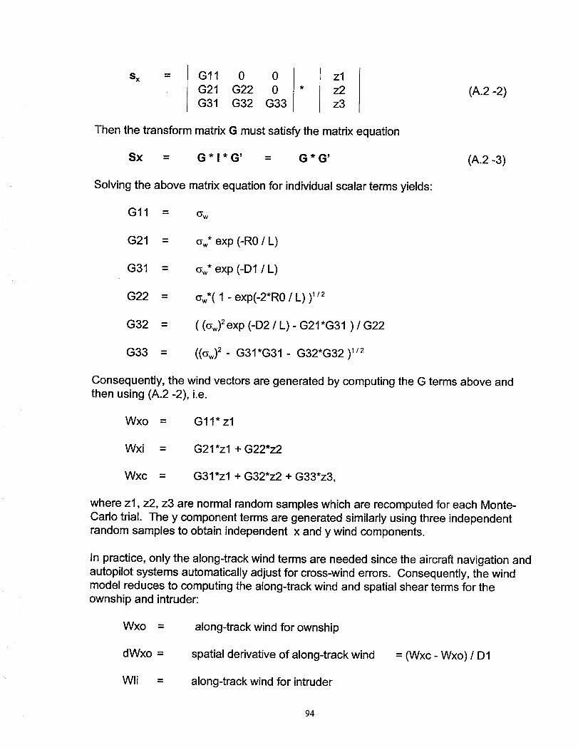
Sx -" Gll 0 0G21 G22 0
G31 G32 G33
zl
z2z3
(A.2 -2)
Then the transform matrix G must satisfy the matrix equation
Sx = G * I * G' = G * G' (A.2 -3)
Solving the above matrix equation for individual scalar terms yields:
Gll = _w
G21 = Cw* exp (-R0 / L)
G31 = _** exp (-D1 / L)
G22 = (_w*( 1 - exp(-2*R0 / L) )1/2
G32 = ( ((_w)2exp (-D2 / L) - G21*G31 ) / G22
G33 = ((aw)2- G31*G31- G32*G32)l/2
Consequently, the wind vectors are generated by computing the G terms above andthen using (A.2 -2), i.e.
Wxo = Gl1" zl
Wxi = G21*z1 + G22*z2
Wxc = G31*z1 + G32*z2 + G33*z3,
where zl, z2, z3 are normal random samples which are recomputed for each Monte-
Carlo trial. The y component terms are generated similarly using three independentrandom samples to obtain independent x and y wind components.
In practice, only the along-track wind terms are needed since the aircraft navigation and
autopilot systems automatically adjust for cross-wind errors. Consequently, the windmodel reduces to computing the along-track wind and spatial shear terms for theownship and intruder:
Wxo = along-track wind for ownship
dWxo = spatial derivative of along-track wind = (Wxc - Wxo) / D1
Wli = along-track wind for intruder
94

dWli
= cos _J * Wxi + sin _ * Wyi
= spatial derivative of along-track wind
= cos _ * (Wxc - Wxi) / D2 + sin _ * (Wyc - Wyi) / D2
The aircraft along-track dynamics for the ownship and intruder are then approximated
by simple differential equations which can be solved analytically:
Ownship Along-Track Dynamics:
The ground speed including wind shear is approximately given by
dx/dt = xo_dot + (x-xo)*dWxo
with xo_dot = V1 + Wxo. Solving the differential equation (A.2-4) yields
x(t) - xo = xo_dot* ( exp ( t * dWxo) - 1) / dWxo
x_dot ( t ) = xo_dot * exp ( t * dWxo )
Approximating the exponential above by a first order Taylor series yields
x_dot (t) ~ ( V1 + Wxo )( 1 + t * dWxo ) Ownship speed
x ( t ) - xo - ( V1 + Wxo )( t + (t2/2) * dWxo ) Ownship distance
Intruder Alonq-Track Dynamics:
The intruder dynamics and closed form predictions are similar to those above:
Li_dot ( t ) = V2 + Wli + ( Li - Lo ) * dWli
Li( t ) - Lo ~
( V2 + Wli ) ( 1 + t * dWli) Intruder speed
( V2 + Wli ) ( t + (t2/2) * dWli) Intruder distance
(A.2-4)
(A.2-5)
(A.2-6)
where in the above expressions, xo and Lo denote the along-track axes at the entry fix,
x( t ) and Li ( t ) denote along-track distances as functions of time since arrival at theentry fixes, and x_dot (t) and Li_dot (t) denote the corresponding ground speed.
95
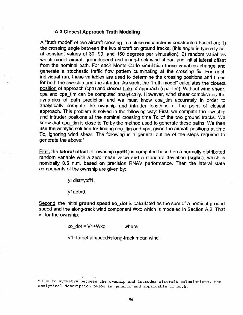
A.3 Closest Approach Truth Modeling
A "truth modei" of two aircraft crossing in a close encounter is constructed based on: 1)
the crossing angle between the two aircraft on ground tracks; (this angle is typically setat constant values of 30, 90, and 150 degrees per simulation), 2) random variableswhich model aircraft groundspeed and along-track wind shear, and initial lateral offset
from the nominal path. For each Monte Carlo simulation these variables change andgenerate a stochastic traffic flow pattern culminating at the crossing fix. For eachindividual run, these variables are used to determine the crossing positions and timesfor both the ownship and the intruder. As such, the "truth model" calculates the closest
position of approach (cpa) and closest time of approach (cpa_tim). Without wind shear,cpa and cpa_tim can be computed analytically. However, wind shear complicates the
dynamics of path prediction and we must know cpa_tim accurately in order toanalytically compute the ownship and intruder locations at the point of closestapproach. This problem is solved in the following way: First, we compute the ownship
and intruder positions at the nominal crossing time Tc of the two ground tracks. Weknow that cpa_tim is close to Tc by the method used to generate these paths. We then
use the analytic solution for finding cpa_tim and cpa, given the aircraft positions at timeTc, ignoring wind shear. The following is a general outline of the steps required togenerate the above: 1
First, the lateral offset for ownship (yoffl) is computed based on a normally distributed
random variable with a zero mean value and a standard deviation (siglat), which isnominally 0.5 n.m. based on precision RNAV performance. Then the lateral state
components of the ownship are given by:
yl dist=yoffl,
yldot=0.
Second, the initial ground speed xo_dot is calculated as the sum of a nominal groundspeed and the along-track wind component Wxo which is modeled in Section A.2. That
is, for the ownship:
xo dot = Vl+Wxo where
Vl=target airspeed+along-track mean wind
z Due to symmetry between the ownship and intruder aircraft calculations, the
analytical description below is generic and applicable to both.
96

Third, the nominal along track position xldist and velocity xldot at time Tc is a function
of the distance between the aircraft at the entry point and crossing fix (D1), the mean
crossing time (Tc), and the wind shear (dwxo). That is:
xldist=-Dl+xo_dot*(1 +a/2+a2/6)*Tc and
xldot=xo_dot*(1 +a+a2/2) where
a=dwxo*Tc
D I=VI*Tc
Note: Nominal values for the above parameters are: mean cross_time=25 min; target
airspeed =480 knots; mean wind magnitude=40 knots; mean wind angle=-45 deg.
The calculations for the intruder states at time Tc are similar, except that we also rotate
from along-track to x-y coordinates.
Fourth_, ¢pa_tim and cpa are calculated by using the relative intruder geometry shown
in Figure A-3:
cpa_tim = -Rc*Rcdot/delvsq + Tc
cpa = Rc*(1-Rcdot2/delvsq)l_2sign(cross)
cross = delx*delydot-dely*delxdot
Rc = (delx 2 + dely2) 1/2
Rcdot = (delx*delxdot + dely*delydot)/Rc
delx = x2dist - xldist
dely = y2dist - yldist
delxdot = x2dot - xldot
delydot = y2dot - yldot
delvsq = (delxdot) 2 + (delydot) 2
where
97
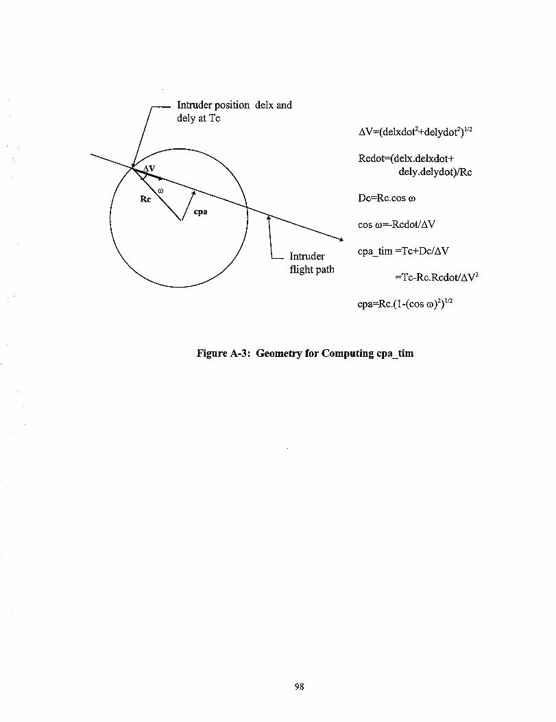
/ Intruder position delx and
_ fl_ght path
AV=(delxdotZ+delydot 2)1/2
Rcdot=(delx.delxdot+
dely.delydot)/Rc
Dc=Rc.cos 03
cos 03=-Rcdot/AV
cpa_tim =Tc+Dc/AV
=Tc-Rc.Rcdot/AV 2
cpa=Rc.(1-(cos 03)2)1/z
Figure A-3: Geometry for Computing cpatim
98

A.4 Surveillance System/Tracker Noise Modeling
The traffic model consists of modeling the trajectory for both an Ownship and anIntruder aircraft. Their position and velocity is estimated by a tracker which introduces
both position and velocity errors relative to each observation point. This model utilizesthe aircraft trajectory information embedded in the flight plan and fuses it with the
tracker observations. Only the along-track surveillance information is retained for pathpredictions. In the context of a Monte Carlo simulation of the above traffic model,tracker noise associated with these observations needs to be modeled as an additional
error source that contributes to the total prediction uncertainty for both the Ownship andIntruder aircraft.
To generate the tracker noise for along-track performance requires the following
concepts and relationships:
Let the true along-track position and velocity of an aircraft be denoted by:
s, = (x,, v,)T
and let the estimated position and velocity due to radar/tracker surveillance be denotedby:
Slt- (X't, V't) T
the error then is defined as the difference between the true and estimate:
et = s t - s' t = (x t - X't, V t - V' t )
We assume here that the tracker can be modeled using a steady state o_-13filter as
defined by Kalata 2, i.e. _ and 13are the filter coefficients associated with the steady
state position and velocity gains Kx and Kv.
The mean and covariance of the error et at each observation time t are given by:
Ee t = O.
and
Eete T = S = o-2D where
2 For more details see for example, Paul R. Kalata "The Tracking Index: A
Generalized Parameter for _-_ and _-_-y Target Trackers", in IEEE Transactions
On Aerospace and Electronic Systems Vol. AES-20. No. 2 March 1984.
99
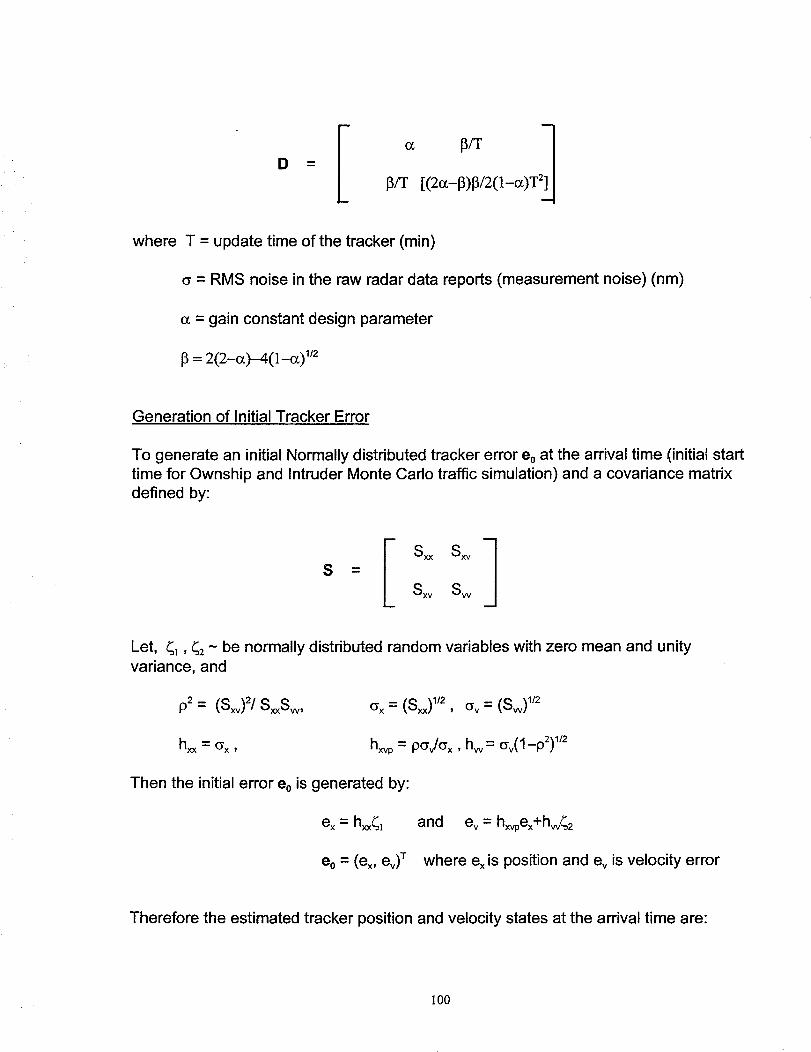
D
13fr
where T = update time of the tracker (min)
(_ = RMS noise in the raw radar data reports (measurement noise) (nm)
cc= gain constant design parameter
= 2(2_o0__4(1_c01/2
Generation of Initial Tracker Error
To generate an initial Normally distributed tracker error e0 at the arrival time (initial starttime for Ownship and Intruder Monte Cado traffic simulation) and a covariance matrix
defined by:
S _.
I Sx_ Sxv 1Sxv Sw
Let, _1, G - be normally distributed random variables with zero mean and unityvariance, and
p2= (Sxv)2/Sx_Sw, _x= (Sxx)''_ , (,v= (Svv)1'_
hx_= _x, hxvp= P(_JOx, hvv= (yv(1-p2) '/2
Then the initial error e0 is generated by:
ex = hxx_l and ev = hxvpex+hw_2
eo = (e×, ev) T where ex is position and ev is velocity error
Therefore the estimated tracker position and velocity states at the arrival time are:
100

x'0 =x0-ex and v'o =v0-ev
Recursive Generation of Tracker Errors at Probe Update Times
Now, suppose that the conflict probe performs conflict detection at intervals of • =mT
(for example, m=6 if T=1/6 min, _=1 min). Then the tracker noise is correlatedfrom one update to the next update interval. It can be shown that (Bryson 3, section
11.2) correlation between et at the current time and et._T at the last update satisfiesthe recursion:
Or. = Ee t"eXt.mT= A"Cm.1 = A m"Co (A.4-1)
where Co = S and
We will use this equation to derive a recursive formula for tracker noise et given the last
error state et-,,T as:
e t = F m" et.mT + G (A.4-2)
where Fr, and G are constant 2X2 matrices, and nl and n2 are independent Normal(Gaussian) random variables with zero mean and unity variance.
Now, from equation (A.4-2) we find that the covariance of the current and the last errorstate is given by:
C,, = Eet" et_ T = F,," (Eet.mT"e'rt-mT)+ 0
- =FIn'S
or Fm= C,," S1 = (Am-S)-S 1 = A m (A.4-3)
3 See section 11.2 in Bryson, A. E., Ho, Yu-Chi Applied Optimal Control,
Blaisdell 1969.
101

Similarly, the covariance of et is given by:
S = Ee t"eTt = Eet(eTt.mT • FTm + (nl, n2)G T)
S = CmFTm + E(Fmet.mT + G In 1_ =,m,,,i
S = Fro"SFTm + GG T
)(nl, n2)G T
(A.4-4)
without loss of generality we can assume that G has the special form:
G ,_
Gx 0 1Gxv Gv
then, from (A.4-4) we find that
G-G T --
I G2x GxGxvGxGxv G2v + G2xv
S - Fm'S" FTm = Q (A.4-5)
solving for the components of G yields:
Gx = (Qx_) 1/2, Gxv = Qxv/Gx, Gv = (Qvv- G2xv) 1/2 (A.4-6)
Now, the solution method for obtaining Fm and G given by equations (A.4-3) thru (A.4-6)
reduces to the following:
Step 1: Recursively generate Fro:
The matrix equation F m - A Fro.1 reduces to the following four scalar equations:
F11(m ) = (1-c_)(F_(m-1) * TF2_(m-1))
102
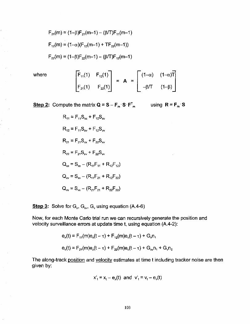
where
F21(m ) = (l-_)F2_(m-l)- (_/T)F_(m-I)
F,2(m) = (1-o_)(F_2(m-l)+ TF=(m-I))
Fz_(m) = (I-_)Fz2(m-I ) - (_/T)F _2(m-I )
j E_(I) F_2(1) (I-o_) (I--_)= a =
LF2,(i ) Fz_(l -_FF (I-_1]
Step_2: Compute the matrix Q = S - F,.'S'FTr. using R =Fm "S
Rll = FllSxx + F12Sx_
R12 = FllSxv + F12Sw
R21 = F21Sxx + F22Sxv
R_ = F21Sxv + F_Sw
Qxx = Sx. - (RllFll + R12F12)
Qxv = Sxv - (RllF21 + R12F_)
Qw = Sw - (R21F21 + R_F_)
Ste__3: Solve for Gx, Gxv, Gv using equation (A.4-6)
Now, for each Monte Carlo trial run we can recursively generate the position and
velocity surveillance errors at update time t, using equation (A.4-2):
e×(t) = Fll(m)ex(t- _) + F_2(m)ev(t--c) + Gxn_
ev(t) = F21(m)ex(t - _) + F_(m)ev(t - _) + Gxvnl + Gvn2
The along-track position and velocity estimates at time t including tracker noise are then
given by:
x't = xt- ex(t) and v't = vt- e_(t)
103

A.5 Estimated Closest Approach Modeling
Section A.3 described the "truth model" which generates the appropriate parameters
that define the modeled trajectories, times, and positions in space for both the ownshipand intruder. This section describes the estimated/predicted or observed/measured
flight path parameters for both the ownship and intruder. The simulation models theownship and intruder conflict detection performance in the midst of uncertainties
introduced by surveillance errors, wind and wind shear estimates, and other error
sources (e.g. Flight Technical Errors). In the context of these uncertainties an estimated.(observed) closest approach position cpa_o and time cpa_tim_o are calculated as the
basis for the conflict detection algorithms.
It is assumed that the aircraft will follow the current flight plan with small lateral
tolerances. Consequently, we can discard the lateral position and velocity states fromthe tracker in favor of the known flight plan based ground track, and use only the along-track position and velocity states for medium term predictions. Suppose 4/o and 4,,
denote the ground track angles relative to North in a NED 4 system for the ownship and
the intruder aircraft. The ownship and intruder velocity components at prediction time At
are approximated by:
Vxo(At) = Vo(l+AtSf)cOS_o (A.5-1)
Vyo(At) = Vo(1+AtSf)sin_o
Vx,(At) = v,(1 +AtS'f)cos_,
vy,(At) = v,(l+AtS'f)sin%
where Vo and v, denote the current ground speed estimates for the ownship and intruder(including tracker noise), and Sf, Sf' denote the wind shear forecasts over the prediction
period along the ownship and intruder flightpath (See A.2-4 to A.2-6). There are twosources of wind shear forecast error: 1 ) time correlated errors due to forecast data timelag, and 2) position or grid related errors due to observation errors at discrete points.
The time correlated errors will tend to be highly correlated in time and distance and are
represented by an exponential correlation. The grid related errors are more likeindependent noise sources which will result in shorter correlation lengths when
interpolating winds across a grid system. A simple method to represent these sourceswas used in the Monte Carlo simulation, i.e. if ST denotes the true along-track windshear, then the forecasted wind shear Sf is modeled as:
Sf = bST+cs_ where,
4 NED is North, East, Down convention (right hand rule).
104

b is a gain constant with nominal value b=0.75, _ is a normal (0, 1) random variable and
_s is a wind shear error constant with numerical value _s = 0.0005 which corresponds to
3 knots wind error per 100 nm:
0.0005per min = (3 kts)/(100 nm)(60 min)
The b constant is chosen to obtain the desired level of exponentially correlated noise
corresponding to forecast lag, and the _s constant is chosen to represent the
measurement error in the grid interpolation process.
Integrating the above velocity equations (A.5-1) yields the position components whichare:
Xo(At) = Xo+Vo(At+At2Sf/2)cOS_o (A.5-2)
Yo(At) = Yo+Vo(At+At2Sf/2)sin_o
x,(At) = x,+v,(At+At2Sf/2)cos_
y_(At) = y_+v_(At+At2Sf'/2)sin_,
where (xo, Yo) and (x,, y_)denote the current horizontal position of the two aircraft asprojected onto their intended ground track. Now from the velocity estimates (A.5-1) andposition (A.5-2) component equations we obtain the predicted position of the intruderrelative to the ownship:
Ax(At) = (XcXo)+(v_cos_,-VoCOS_o)At+(v_Sf'cos_-VoSfCOS_o)At2/2 (A.5-3)
Ay(At) = (ycyo)+(v,sin_-VoSin_o)At+(v,Sf'sin_,-VoSfsin_o)At2/2
AVx(At) = (v,cos_-VoCOS_o)+At(v,Sfcos_t-VoSfCOS_o)
Avy(At) = (vtsin_,-VoSin_o)+At(v,Sf'sin_j-VoSfsin_o)
We now obtain an implicit equation and a two step iteration for the time of minimum
approach tm_,,for two converging aircraft (R_dot<0). From (A.5-3), the predicteddistance-squared for the two aircraft as a function of At is given by:
R2(At)= AX2(At)+Ay2(At) (A.5-4)
105

=(_o+AtAVx(At/2))2+(AYo+AtAvy(At/2)) 2
where _x o = xt-Xo, AYo = Y_-Yo. Differentiating (A.5-4) to find the minimum distance yields
an orthogonality condition at At = train:
0 = (_Xo+tminAVx(tmJ2))AVx(tmin)+(AYo+tminAVy(tm_n/2)AVy(tm_n) (A.5-5)
Solving (A.5-5) for trninyields the _ equation:
trn_n= -(z_aVx(tmin) + AYoaVy(tmin))1 (A.5-6)
(AVx(tm,n/2)AVx(tmin) +AVy(tmin/2)Avy(tm,n))
In practice, this equation can be solved in a few iterations or alternatively by analytically
solving the cubic equation for tm_oin (A.5-5). Ignoring the wind shear terms yields aninitial estimate:
tl = -(AxoAvx(0)+AYoAVy(0))/(AVx2(0)+Avy2(0)),
tin,, = -(AXoAVx(tl)+AYoAVy(t_))/
(AVx(t_/2)Avx(t_)+Avy(t_/2)Avy(tl)).
and then
The min distance or cpa_o is then obtained from (A.5-4):
Rmin = cpa_o = (R2(t=,o)) 1'2 (A.5-7)
The following is a list of the equations used to calculate cpa_tim_o and cpa_o. The
definition of these variables are provided in the Nomenclature. First, the observed
velocity and forecasted wind shear are computed using:
vgndop=vgndo-Ev
vgndip=vgndi-E2v
dwxop=Fore_const*dwxo+sig_shear*N(0, 1)
dwxip=Fore_const*dwxi+sig_shear*N(0, 1)
where N(0, 1) denotes a Gaussian random variable with mean zero and unit variance.
Then the observed relative position and velocity states are calculated:
106

sldist_o = -D1 +vgndop*(dt+dwxop*dt2/2)+Ex
s2dist_o = -D2+vgndip*(dt+dwxip*dt2/2)+E2x
sldot_o = vgndop*(1 +dwxop*dt)
s2dot_o = vgndip*(l+dwxip*dt)
delx o = s2dist o*costhe-sldist o
dely_o = s2dist_o*sinthe
delxdot o = s2dot o*costhe-sldot o
delydot_o = s2dot_o*sinthe
The first iteration for cpa_tim_o is then given by:
dotp = delx_o*delxdot_o+dely*delydot_O
delvsq_o = delxdot_o2+delydot_o 2
timo = -dotp/delvsq_o
The first iteration for cpa_tim.o is then calculated:
templ= s2dot_o*dwxip*costhe-sldot_o*dwxop
tempx = timo*templ
delvx2 = delxdot_o+tempx/2
delvx=delxdot_o+tempx
temp2=s2dot_o*dwxip*sinthe
tempy=timo*temp2
delvy2 = delydot_o+tempy/2
delvy=delydot_o+tempy
denom= delvx2*delvx+delvy2*delvy
107

cpa_tim_o = -(delx_o*delvx+dely_o*delvy)/denom
Finally, the estimated cpa is given by:
delx2 = delx_o+cpa_tim_o*delvx2
dely2 = dely_o+cpa_tim_o*delvy2
cross_o = delx2*delvy-dely2*delvx
delv = (delvx 2 + delvy2) _/2
cpa_o = (delx22+dely22) 1/2*sign(cross_o)
108
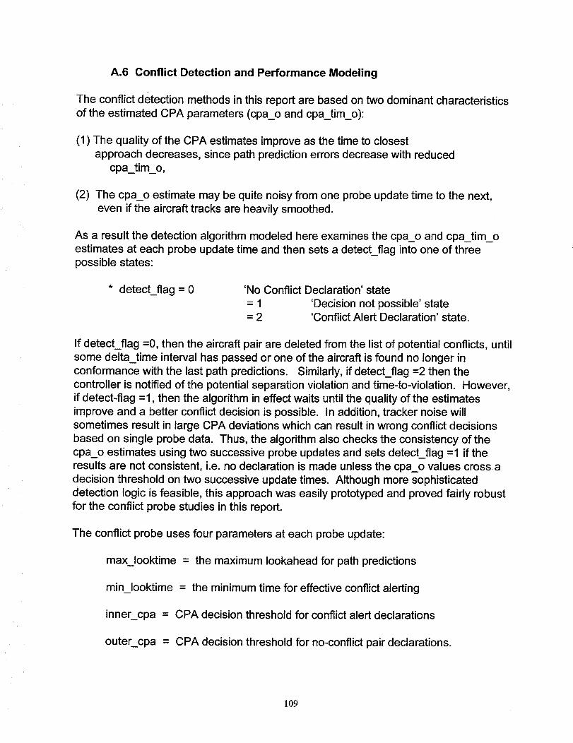
A.6 Conflict Detection and Performance Modeling
The conflict detection methods in this report are based on two dominant characteristics
of the estimated CPA parameters (cpa_o and cpa_tim_o):
(1) The quality of the CPA estimates improve as the time to closest
approach decreases, since path prediction errors decrease with reducedcpa_tim_o,
(2) The cpa_o estimate may be quite noisy from one probe update time to the next,
even if the aircraft tracks are heavily smoothed.
As a result the detection algorithm modeled here examines the cpa_o and cpa_tim_oestimates at each probe update time and then sets a detect_flag into one of threepossible states:
* detect_flag = 0 'No Conflict Declaration' state
= 1 'Decision not possible' state= 2 'Conflict Alert Declaration' state.
If detect_flag =0, then the aircraft pair are deleted from the list of potential conflicts, until
some delta_time interval has passed or one of the aircraft is found no longer in
conformance with the last path predictions. Similarly, if detect_flag =2 then thecontroller is notified of the potential separation violation and time-to-violation. However,if detect-flag =1, then the algorithm in effect waits until the quality of the estimates
improve and a better conflict decision is possible. In addition, tracker noise willsometimes result in large CPA deviations which can result in wrong conflict decisions
based on single probe data. Thus, the algorithm also checks the consistency of thecpa_o estimates using two successive probe updates and sets detect_flag =1 if theresults are not consistent, i.e. no declaration is made unless the cpa_o values cross a
decision threshold on two successive update times. Although more sophisticateddetection logic is feasible, this approach was easily prototyped and proved fairly robust
for the conflict probe studies in this report.
The conflict probe uses four parameters at each probe update:
max_looktime = the maximum Iookahead for path predictions
min_looktime = the minimum time for effective conflict alerting
innercpa = CPA decision threshold for conflict alert declarations
outercpa = CPA decision threshold for no-conflict pair declarations.
109

Once the estimated cpa_o and cpa_tim_o are computed for a potential conflict pair, thefollowing steps are applied:
(1) cpa_tim_o checking:
If cpa_tim_o > max_looktime, then the quality of the CPA parameters is questionable
and consequently we set detect_flag =1. Similarly, if cpa_tim_o < min_looktime (wheremin_looktime is less then or equal to the Iookahead time for the Short Term Conflict
Alert algorithm), then the conflict pair is being managed by the sector controller and weset detect_flag = 1 to take no further action. Otherwise, if cpa_tim_o is within thesetime limits we proceed to step (2).
(2) conflict status detection logic:
If cpa_o< inner_cpa on two successive probes, then we declare a conflict alert, i.e.
detect_flag = 2. The innercpa threshold is chosen at some value exceeding the
separation standard, i.e. for the fixed threshold algorithm when sep_std = 4, we typicallyset inner_cpa = 5 nm, in order to keep the probability of missed detections less than2%. (See Figure A-3.) The covariance method and conformance method algorithms
select the inner_cpa dynamically, depending on CPA uncertainty and conflict geometry,whereas the fixed threshold method selects inner_cpa based on worst case conditions
at maximum Iookahead and at crossing angles of 20 - 30 deg.(For further details on relative performance of these algorithms see Section 4.)
If cpa_o > outer_cpa on two successive probes, then we declare this pair conflict free,i.e. detect_flag = 0. The outer_cpa threshold should be selected large enough toprevent an excessive number of false alerts, and significantly larger than the
inner_threshold in order to avoid missed detections. However, the outer_cpa thresholdshould change dynamically with CPA uncertainty, in order to minimize the number of
false alerts when CPA can be estimated accurately. For the fixed threshold algorithm,we set outer-cpa larger than the intervention standard (See Figure A-3), so that thealgorithm performs well in worst case conditions. The covariance method selects the
outercpa threshold dynamically, and typically does not begin making any decisionsuntil outer_cpa is slightly larger than the intervention standard. Both the outer and inner
thresholds then vary dynamically with approach time. (See Figure 5).
If neither of the above conditions holds, then detect_flag=l, and the current estimatesof cpa_o and cpa_tim_o are stored for use on the next probe update.
The performance of the conflict detection algorithms is assessed by counting thenumber and percentage of missed detects and false alerts, and by evaluating warningtime statistics, where warning time is the estimated time remaining until a separationviolation occurs, measured from time of first alert. For each Monte Carlo run, we first
determine the detect_flag status when the conflict probe ended, and the truth cpa
status as defined by the following 'truth_flag' :
110
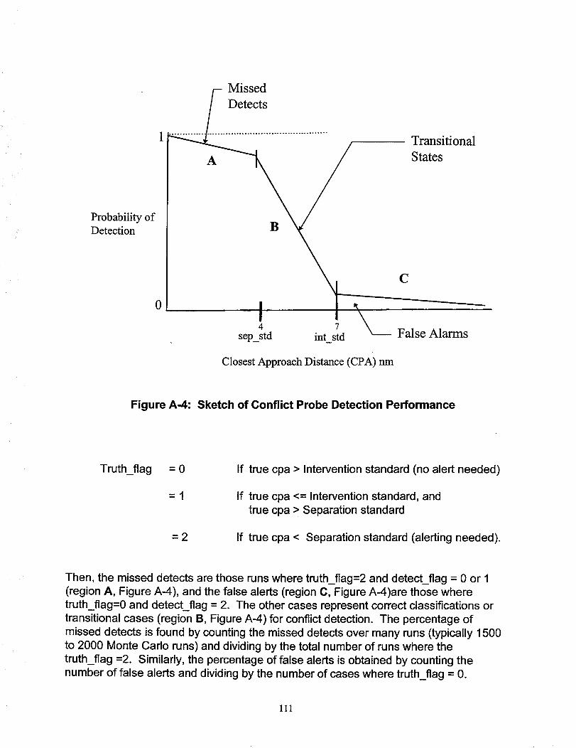
Missed
Detects
A
Transitional
States
Probability ofDetection B
0 I
C
4 7False Alarmssep_std int std
Closest Approach Distance (CPA) nm
Figure A-4: Sketch of Conflict Probe Detection Performance
Truth_flag =0
=1
=2
If true cpa > Intervention standard (no alert needed)
If true cpa <= Intervention standard, and
true cpa > Separation standard
If true cpa < Separation standard (alerting needed).
Then, the missed detects are those runs where truth_flag=2 and detect_flag = 0 or 1
(region A, Figure A-4), and the false alerts (region C, Figure A-4)are those where
truth_flag=0 and detect_flag = 2. The other cases represent correct classifications or
transitional cases (region B, Figure A-4) for conflict detection. The percentage of
missed detects is found by counting the missed detects over many runs (typically 1500
to 2000 Monte Carlo runs) and dividing by the total number of runs where the
truth_flag =2. Similarly, the percentage of false alerts is obtained by counting the
number of false alerts and dividing by the number of cases where truth_flag = 0.
111

A more detailed picture of conflict probe performance can be presented as a histogram
of conflict detection probability as sketched in Figure A-4, but this level of detail is notneeded for most conflict probe studies.
In our studies, warning time is computed as the time from first alert until the separationis equal to the inner_cpa threshold. This time is computed when detect_flag=2 using
warn_time = cpa tim_o - ( ((inner_cpa) 2 - (cpa_o) 2 )/delv 2)_/2
where delv is an intermediate quantity representing the relative velocity between the
ownship and the intruder in the CPA calculations in Section A.5.
A.7 Monte Carlo Performance Evaluations
In order to assess the accuracy levels required for the estimation of the probabilities ofMissed Detection and False Alarm in the Conflict Probe study, the convergence of their
average values after a number of Monte Carlo simulations was evaluated for a fixedthreshold conflict probe logic concept configured with a separation standard of 3 nm,
inner threshold of 3 nm, outer threshold (and outlier) of 5 nm, and a Iookahead time of20 min. Two basic approaches were taken: 1) the running average probabilities were
computed for sets of n Monte Carlo simulations represented by an average over anensemble of n runs. For example, Figures A-5 through A-8 show convergence forn=900 and n=1800 derived from a total number of N=6000 runs; 2) the cumulative
convergence of the probabilities of Missed Detection and False Alarm is shown in
Figures A-9 and A-10.
The running average method for the probability of missed detection shows the
results of averaging over n=900 (Figure A-5). At this relatively low sample size, theconvergence of the final value of average probability of missed detects is not robust asexemplified by the lack of data in some of the ensemble averages. As a general
reference, however, the overall average value of missed detect probabilities over thetotal ensemble average is 0.94% indicating that even at this low ensemble sample size
the average of the variations in the probability of missed detects is less than 1%. Whenthe ensemble average is doubled to n=1800 (Figure A-6), the missed detect
probabilities show significantly less variation, although the average of the total set ofensembles for this case is 0.95%, not significantly different from the n=900 results. Itmay be concluded that n=1800 is minimally adequate to predict a fairly robust value for
the probability of missed detect performance of the conflict probe model.
Similarly, for the probability of false alarms compiled with the running averagemethod, the statistical results are summarized in Figures A-7 and A-8 for the ensemble
running averages of n=900 and n=1800, respectively. The average probability of false
alarms for both cases was about 3% although the statistical variation of the ensemble
112

averages is greater for the n=900 case in Figure A-7 as compared to the n=1800 caseshown in Figure A-8. Regardless of the variations, these results indicate that the rate of
false alarms is estimated to a precision better than1% with n>=1800 samples.
The other method of evaluating the statistical convergence characteristics of the MonteCarlo simulation used the cumulative convergence method. The convergence
statistics for the missed detect probability is shown in Figure A-9. The results indicate
that a final estimated value of the probability of missed detects settles approximately at1% after about n=1800 to n=2000 Monte Carlo simulations. This generally confirms the
conclusions of the above running average mode of evaluation. Similarly, Figure A-10
shows the cumulative convergence of the probability of false alarms. The variation inthe statistics begin to settle at an approximate final value of 1.8% after about n=2000Monte Carlo simulations.
Given the above general findings on the statistical convergence characteristics for both
missed detect and false alarm performance, the conflict probe studies were generallyconducted with a minimum of 1800 Monte Carlo runs. In some cases, a greater number
of cases were required to attain better robustness and convergence performance.
113
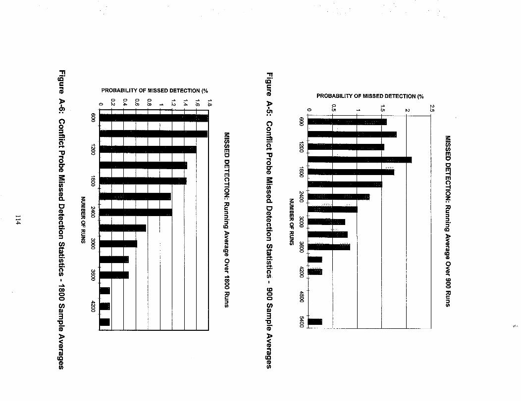
-rl "11
" c
PROBABILITY OF MISSED DETECTION (% _ PROBABILITY OF MISSED DETECTION (%
.- ,, ol°_ _ mmmmm [] ) _ mmm
"_ _p=..........m = _ ._ _.,,=m_, ==g mmm mm _ g )_mmm
mmmmmmm ) ) mm ),', _ ! '" ,., _ ..
mm, o _ o
o o g
(p (P

4
FALSE ALARM STATISTICS:
Average Over 900 Runs
600 1200 1800 2400 3000 3600 4200 4800 5400
NUMBER OF RUNS
Figure A-7: Conflict Probe False Alarm Statistics - 900 Sample Averages
3.5
FALSE ALARM STATISTICS:
Average Over 1800 Runs
3
n,"_ 2.5_1
I,LIO0-- 2
U.
0 1.5
,-1
m 1<_mO
o.. 0.5
600 1200 1800 2400 3000 3600 4200
NUMBER OF RUNS
Figure A-8: Conflict Probe False Alarm Statistics - 1800 Sample Averages
115
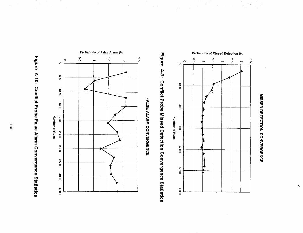
O',
"11m,
tOr-g
,>,=_
=l
(3O
m=
(3
"oaO"(I)"11¢gm
U)
m
¢g
3C)O
<
=3
(3(D
(n
ml
U)¢,.,Fm=
(3U)
Ze.
3cr
o_.;0r'.=3(/1
O
O
O
O
O
8
g
C,3OOO
C_O1OO
,._000
0
Probability of False Alarm (%
O --_
_ Cn to O1
j.'#
_ "dl,
A
"e
I _K_
:\i
"1"1
i-(nm
r-
;0i:(3OZ<m30G)mZ(3m
"11m.
¢2¢..
g_>
i=
C)O
ml
(3
"oaO"(I)
i:m=
U)(n(DO.
[3
(I)(3ml
O
C)O
<(D
_Q
(3¢D
(n93e=Fm=
Ulm=
(3Ul
O
00
tO000
ZC
3
_ N_ 8
C
000
000
0)000
0
Probability of Missed Detection (%
0 _ to
S7
E
01
N
(n(/)mC_C_m-Im(3-I
0Z(3OZ<m;0
mzom

Appendix B: Conflict Probe Covariance Analysis
This section derives the math equations underlying the covariance based conflict probe.(See Section 4.1 for an overview of the technical approach.) Section B.1 derives the
longitudinal (along-track) covariance uncertainty for medium term path predictions.Section B.2 derives the two-dimensional covariance uncertainty for an intruder aircraft,relative to a reference or "ownship" aircraft path, explicitly using the equations in
Section B.1. Section B.3 applies the results of Section B.2 to obtain dynamic equationsfor conflict detection and no-conflict decision thresholds, based on predicted path
covariance uncertainty. Section B.4 derives an expression for predicted probability ofloss-of-separation between two aircraft. This variable may be useful operationally, for
planning conflict resolution tactics and for timing conflict resolutions, i.e. whether to act
now to prevent a potential conflict, or to wait until the conflict situation becomes clearer.Section B.5 derives precise equations for predicting the start and end times for crossing
/ opposing and limited duration in-trail path conflicts.
B.1 Longitudinal Prediction Error Modeling - Cruise Flight
In this section we model the error dynamics for longitudinal flight predictions. Threeerror sources are modeled in our analysis:
* surveillance estimation error on along-track position and velocity states,* wind - forecasting error, including the effect of horizontal wind shear,
* longitudinal speed-following Flight Technical Error (FTE).
This section provides a condensed derivation of covariance formulae for estimating
longitudinal prediction uncertainty as a function of prediction time. In our studies, thespeed following error terms were deleted, since the surveillance and wind forecasting
errors typically dominate the steady state speed following errors. However, the speedfollowing errors for manually flown flight can be on the order of three knots rms (Ref.12), and should be included for completeness.
The basis of our error model are three differential equations which describe the
evolution of prediction errors as a function of prediction time t. The first equation is apartition of the predicted ground speed x_dot = Vx (t) into several components:
Vx = Va + Wf(x) +Wx (B.1- 1)
where
Vx = predicted ground speed at time tVa = along-track true air speed at time t
Wf(x) = forecasted along-track wind at position x(t)Wx = along-track wind forecast errorx (t) = predicted along-track path location at time t.
117
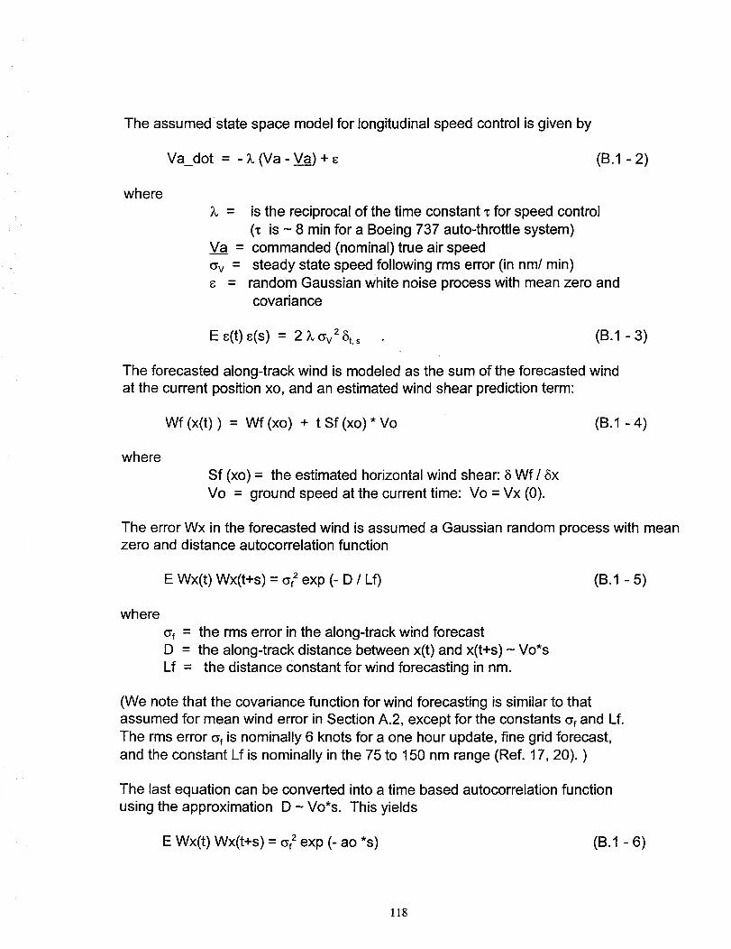
The assumed-state space model for longitudinal speed control is given by
Va_dot = - X (Va - V__aa)+ s (B.1 -2)
where
Va =
O"v =
S =
is the reciprocal of the time constant x for speed control
(_ is - 8 min for a Boeing 737 auto-throttle system)
commanded (nominal) true air speedsteady state speed following rms error (in nm/min)
random Gaussian white noise process with mean zero andcovariance
E s(t) s(s) = 2 ;L(_v2 8t.s (B.1 - 3)
The forecasted along-track wind is modeled as the sum of the forecasted wind
at the current position xo, and an estimated wind shear prediction term:
Wf(x(t)) = Wf(xo) + tSf(xo)*Vo (B.1-4)
where
Sf (xo) = the estimated horizontal wind shear: 5 Wf / 8x
Vo = ground speed at the current time: Vo = Vx (0).
The error Wx in the forecasted wind is assumed a Gaussian random process with meanzero and distance autocorrelation function
E Wx(t) Wx(t+s) = (_ exp (- D / Lf) (B.1 - 5)
where
O'f --
D=Lf =
the rms error in the along-track wind forecast
the along-track distance between x(t) and x(t+s) - Vo*sthe distance constant for wind forecasting in nm.
(We note that the covariance function for wind forecasting is similar to thatassumed for mean wind error in Section A.2, except for the constants (_fand Lf.
The rms error (_f is nominally 6 knots for a one hour update, fine grid forecast,
and the constant Lf is nominally in the 75 to 150 nm range (Ref. 17, 20). )
The last equation can be converted into a time based autocorrelation function
using the approximation D ~ Vo*s. This yields
E Wx(t) Wx(t+s) = (_f2exp (- ao *s) (B.1 -6)
118

with ao = Vo / Lf. This transformation enables us to express Wx (t) as a stationary
process generated by a random differential equation
Wx_dot = - ao * Wx + 1] (B.1 - 7)
where 1"1is a white noise process with mean zero and covariance
E _l(t) Tl(S) = 2 ao of 2 5t.s (B.1 - 8)
We now obtain an explicit differential equation for x_dot by expanding (B.1 - 1) andusing the definition of Vo:
x_dot (t) = Va + (Wf(xo) + t*Sf(xo) Vo) + Wx(t)
= Vo*( 1 + t*Sf(xo) ) + ( Wx(t)- Wx(0) ) + ( Va(t)- Va(0) ) (B.1 - 9)
Now defining the speed error state 5Va = Va - V._.aa,we can express our error model as a
state space differential equation for (x, 5Va, Wx ):
x_dot = 0*x + _3Va + Wx + g(t) (B.1-10)5Va dot = - ;L 5Va + s
m
Wx_dot = - a Wx + 1"1,
where g(t) = Vo*( 1 + t*Sf(xo)) -c3Va(0) - Wx(0).
The state space model given by (B.1-10) can be solved explicitly using exponential
functions and integrals of exponential functions. This yields the following equation foralong-track position x(t):
x(t) = xo + Vo*( t + Sf(xo)*t^2/2) +[ (1 - exp(-;L t) ) / ;L - t ]* aVa(0) + _ (1 - exp(-X s) )( s (t-s)/X) ds
+ [ (1 - exp(-ao t) ) / ao - t ]*Wx(0) + .[ (1 - exp(-ao s) )(q(t-s)/ao) ds,
where the above integrals are defined over 0 <= s <= t.
Subtracting the estimated position x' (t) = xo' + Vo'*( t + Sf(xo)*t*2/2), where(xo',Vo') denote current aircraft tracker estimates of position and speed, yields thefollowing error equations for predicted position at time t:
8x(t) = 5xo + aVo*(t + Sf(xo)*t^2/2) + (B.1- 11)
[ (1 - exp(-X t) ) / ;L - t ]* 5Va(0) + .[ (1 _ exp(-;L s) )( s (t-s)/;L) ds
+ [ (1 - exp(-ao t) ) / ao - t ]*Wx(0) + _ (1 - exp(-ao s) )(-q(t-s)/ao) ds,
119
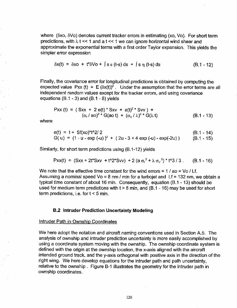
where (Sxo, 5Vo) denotes current tracker errors in estimating (xo, Vo). For short term
predictions, with _ t << 1 and a t << 1 we can ignore horizontal wind shear and
approximate the exponential terms with a first order Taylor expansion. This yields thesimpler error expression
5x(t) = 5xo + t*SVo + j's s (t-s) ds + j's 11(t-s) ds (B.1 - 12)
Finally, the covariance error for longitudinal predictions is obtained by computing theexpected value Pxx (t) = E (Sx(t)) 2 . Under the assumption that the error terms are all
independent random values except for the tracker errors, and using covarianceequations (B.1 - 3) and (B.1 - 8) yields
Pxx (t) = (Sxx + 2 e(t)* Sxv + e(t) 2. Svv) +
((_f / ao) 2 * G(ao t) + (_v / X)2 * G(_. t) (B.1 - 13)where
e(t) = t + Sf(xo)*t^2/2 (B.1 - 14)G(u) = (1 - u - exp (-u))2 + ( 2u - 3 + 4 exp (-u) - exp(-2u) ) (B.1 - 15)
Similarly, for short term predictions using (B.1-12) yields
Pxx(t) = (Sxx+2t*Sxv +tA2*Svv) +2(a_f2+X(_v2)*t^3/3. (B.1-16)
We note that the effective time constant for the wind errors = 1 / ao = Vo / Lf.
Assuming a nominal speed Vo = 8 nm/ min for a turbojet and Lf = 132 nm, we obtain a
typical time constant of about 16 min. Consequently, equation (B.1 - 13) should beused for medium term predictions with t > 8 min, and (B.1 - 16) may be used for shortterm predictions, i.e. for t < 5 min.
B.2 Intruder Prediction Uncertainty Modeling
Intruder Path in Ownship Coordinates
We here adopt the notation and aircraft naming conventions used in Section A.5. The
analysis of ownship and intruder prediction uncertainty is more easily accomplished byusing a coordinate system moving with the ownship. The ownship coordinate system isdefined with the origin at the ownship location, the x-axis aligned with the aircraftintended ground track, and the y-axis orthogonal with positive axis in the direction of the
right wing. We here develop equations for the intruder path and path uncertainty,
relative to the ownship. Figure B-1 illustrates the geometry for the intruder path inownship coordinates.
120
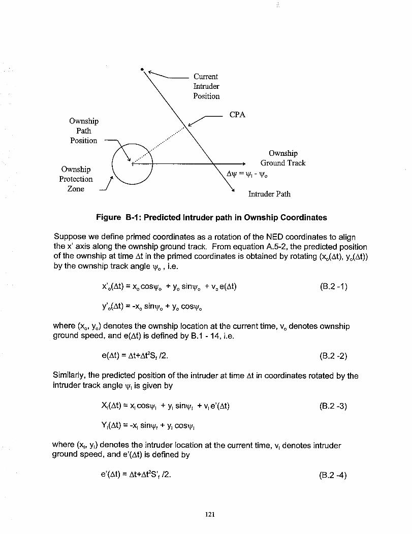
OwnshipPath
Position
Ownship
Protection
Zone
_"-_ Current
Intruder
_ Position
.........,.__,,_ CPA
Ownship
Ground Track
Intruder Path
Figure B-l: Predicted Intruder path in Ownship Coordinates
Suppose we define primed coordinates as a rotation of the NED coordinates to align
the x' axis along the ownship ground track. From equation A.5-2, the predicted position
of the ownship at time At in the primed coordinates is obtained by rotating (Xo(At), yo(At))
by the ownship track angle _o, i.e.
X'o(At) = XocOS_o + Yo sin_o + Voe(At) (B.2 -1)
y'o(At) = -Xo sin_o + Yo cOS_o
where (Xo, Yo) denotes the ownship location at the current time, v o denotes ownship
ground speed, and e(At) is defined by B.1 - 14, i.e.
e(At) = At+At2Sf/2. (B.2 -2)
Similarly, the predicted position of the intruder at time At in coordinates rotated by the
intruder track angle W, is given by
X,(At) = x, cos_, + y, sin_, + v, e'(At) (B.2 -3)
Yl(At) = -xt sinai + Yl cos_,
where (x,, y,) denotes the intruder location at the current time, v, denotes intruderground speed, and e'(At) is defined by
e'(At) = At+At2S'f/2. (B.2 -4)
121

The intruder Position in primed coordinates is then obtained by rotating the aboveequations by _o - % = - A_:
x',(At) = X,(At)cos A_ - Y,(At) sin Au/ (B.2 -5)
y',(At) = X,(At) sin A_ + Y,(At) cos A_
Consequently, the predicted intruder path in ownship coordinates is the difference
between intruder and ownship paths in primed coordinates, i.e. from (B.2 -5) we find
FAx(At)-I = r x',(At)-X'o(At)-ILAy(At)_] Ly',(At)- y'o(At)_]
= [- cos A_ - sin A_ -] I- X,(At) -] - [- X'o(At) -]
L sin A_ cos A_ _JL Y,(At) _1 L y'o(At) _J
(B.2 -6)
This is the fundamental equation needed for analysis of prediction uncertainty.
Error Equations for Intruder Prediction Uncertainty
Now from (B.2 -6) we obtain the following equation for relative intruder path error:
[- 8x(At) -] = [- cos A_ - sin A_F] [- 8X,(At) -] - i- 8X'o(At) -]
L By(At) .J L sin A_ cos A_ J L 8Y,(At) I L 8y'o(At) _J(B.2 -7)
where 8Xf(At), 8Y_(At) denote the longitudinal and lateral prediction errors for the
intruder path, and similarly 8X'o(At), 8Y'o(At) denote the longitudinal and lateral prediction
errors for the ownship path. From the derivation in Section B.1, the ownship predictionerrors can be characterized by the following expressions:
aX'o(At)= aX'o+ e(At)* 8v' o + Oo(At) (B.2-8)
ay'o(At) = %(At) (B.2-9)
where (8X'o, 8V'o) denotes ownship along-track position and velocity surveillance errors,
0o(At) denotes the along-track wind forecasting error, and %(At) denotes the ownship
lateral conformance error relative to the intended ground track. (For simplicity, we areignoring other error sources such as longitudinal speed error.) The error sources are
assumed to be independent random variables (except for cross-correlation betweentracker position and velocity errors), with mean zero and variances given by
Po = E (SX'o+ e(At) * 8V'o) 2 = Sxx + 2 e(At) * Sxv + e(At) 2 * Svv (B.2-10)
Qo = E (Oo(At))2 = (of / ao) 2, G(ao At) , ao = Vo/ Lf (B.2-11)
122

Ro = E (So(At)) 2 = (e_y) 2 (B.2-12)
i.e. the longitudinal errors Po and Qo are functions of At and Ro is a constant.
Similarly, the intruder prediction errors can be characterized by the expression
6X_(At) = 6x, + e'(At)* 6v, + e,(At) (B.2-13)
8Y,(At) = s,(At) (B.2-14)
where (6x_, 6vE)denotes intruder along-track position and velocity surveillance errors,ej(At) denotes the along-track forecasting error, and s_(At) denotes the intruder lateral
conformance error relative to the intended ground track. The variances of the error
components P_,Q_, R_are given by equations analogous to (B.2-10) - (B.2-12).
The wind forecasting errors are assumed to be circular normal with independencebetween x and y component errors, and exponentially correlated errors between distant
forecast points. Thus the random variables Co(At) and Of(At) are cross-correlated,
complicating the estimation of prediction uncertainty. We can express the forecast error0j(At) in terms of x' and y' wind forecast errors in the primed coordinate system:
e,(At) = cos A_ *ex,(At) + sin Atls *e¥,(At) (B.2-15)
where ex_(At) and eyz(At) are independent random variables with mean zero and
variance Q_with
Q_ = (e_f/ a_)2 * G(a_ At) , a_= vi / Lf (B.2-16)
and the cross-correlation between eo(At) and e,(At) is given by
E eo(At)* e,(At) = cos A_s * J o, (B.2-17)
J o, = E eo(At)* ex,(At).
The value of (B.2-15) - (B.2-17) is that the cross-correlation J o_is bounded by thefollowing inequalities:
0 <= Jo_ <= ( Qo* Q_)1/2, (B.2-18)
where the cross-correlation J o_(At)can be shown to be non-negative since the x' axis
wind forecasting errors at each point are exponentially correlated and positive. Theupper bound is a well known property of cross-correlations, i.e. for any two random
123
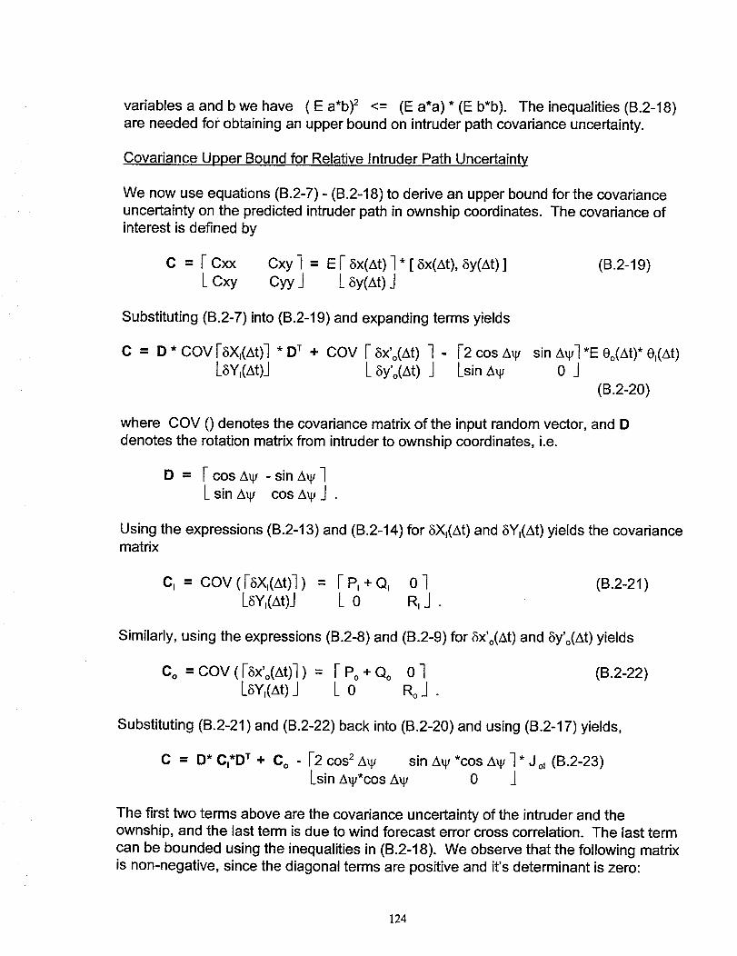
variables a and b we have ( E a'b) 2 <= (E a'a)* (E b'b). The inequalities (B.2-18)are needed fo£ obtaining an upper bound on intruder path covariance uncertainty.
Covariance Upper Bound for Relative Intruder Path Uncertainty
We now use equations (B.2-7) - (B.2-18) to derive an upper bound for the covarianceuncertainty on the predicted intruder path in ownship coordinates. The covariance ofinterest is defined by
C = 1-Cxx Cxy ] = E [- 8x(At) -] * [ 8x(At), By(At) ] (B.2-19)
L Cxy Cyy .j L By(At) J
Substituting (B.2-7) into (B.2-19) and expanding terms yields
c = D* COYI-SX,(At)I* D T + COY [- 5X'o(At ) 1 - I-2cos A_ sin Au/1 *E 0o(At)*e,(At)LSY,(At)/ L 8y'o(At) I Lsin A_ 0 I
(B.2-20)
where COV 0 denotes the covariance matrix of the input random vector, and Ddenotes the rotation matrix from intruder to ownship coordinates, i.e.
D = [-cosA_ -sinAi]
LsinA_ cosA__J .
Using the expressions (B.2-13) and (B.2-14) for 5X_(At) and 8Y_(At) yields the covariancematrix
C, = COV ( [-SX,(At)-] ) = [- P, + Q, 0 ] (B.2-21)LsY,(At)J L 0 R, _J .
Similarly, using the expressions (B.2-8) and (B.2-9) for 8X'o(At) and 5y'o(At) yields
co = coy (I-ax'o(At)-I)= r Po+ Qo 0 1 (B.2-22)LaY,(At)J L 0 RoJ
Substituting (B.2-21) and (B.2-22) back into (B.2-20) and using (B.2-17) yields,
C = D*CI*DT+ Co i-2 cos 2 Au/ sin AW *cos A_ -] * J o_(B.2-23)
Lsin A_*cos AW 0 _J
The first two terms above are the covariance uncertainty of the intruder and theownship, and the last term is due to wind forecast error cross correlation. The last term
can be bounded using the inequalities in (B.2-18). We observe that the following matrixis non-negative, since the diagonal terms are positive and it's determinant is zero:
124

1-2 cos2-A_ sin AW *cos/k_ -I * J o_
Lsin A_*cos A_ sin 2 A_/2 _J
>= 0
Consequently, we can add and subtract the lower right hand term above in (B.2-23) toobtain a covariance upper bound
C = D* C_*DT + Co - I-2 cos 2 A_ sin Au/*cos A_ -] *J oa + [- 0 0 -_* J o_
Lsin z_*cos _/ sin 2 A_/2 _] L0 sin 2 z_/2 _J
<= D* CI*D T + Co ÷ 1-0 0 "] * J oJ
L0 sin 2A_/2j
<= D* C,*D T + Co + 1-0 0 -] * ( Qo* Q,)1/2 (B.2-24)
L0 sin 2 &_/2 _J
Finally, expanding the matrix equation (B.2-24) into it's components yields the followingupper bound on the covariance matrix for intruder prediction uncertainty:
Cxx
Cxy
Cyy
= cos2A_ ( P_+ Q_ ) + sin 2 A_ * R_ + ( Po + Qo )
= sin A_ * cos Au/(P_ + Q_ - R_)
= sin2/k_ ( Pf + Q_ + ( Qo* Q_)1/2/2) + cos2Au/* R_+ Ro
(B.2-25)
Although the derivation of (B.2-25) is lengthy, the calculation above is fairly simple toimplement, and is only needed at the time of minimum approach, i.e. for At =Tmin.
Although an upper bound, the covariance approximation (B.2-25) is a fairly tight boundfor crossing and opposing encounters. For in-trail encounters where the crossing angleis less than 20 degrees, and the relative velocity between conflicting aircraft is small,
the above bound may be overly conservative. However, in this case the solutionmethod for closest approach point and cpa time is not robust, and an alternative
algorithm for slow overtake alerting (longitudinal conformance monitoring) is required.
B.3 Covariance Based Thresholding for Conflict Detection
The thresholding method for covariance based conflict detection requires solving for thecritical point ( 5x*, 5y*) on the predicted uncertainty ellipse at At = Tmin such that the
critical point maximizes the offset distance Runc from the relative intruder path. SeeFigure B-l, below. In the figure below, there is not a potential conflict if Rmin > Rsep +
Runc, since the horizontal separation circle about the ownship does not intersect withthe predicted intruder path uncertainty ellipse as the intruder transits the point of closestapproach. We here derive analytic equations for covariance based thresholding.
125
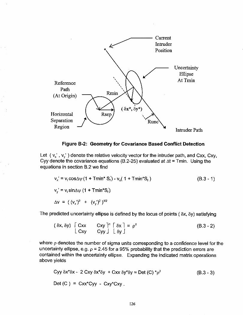
Reference
0
Path
(At Origin)
Horizontal
Separation
Region
Current
Intruder
Position
Uncertainty
Ellipse
At Tmin
Intruder Path
Figure B-2: Geometry for Covariance Based Conflict Detection
Let ( Vx', vy' ) denote the relative velocity vector for the intruder path, and Cxx, Cxy,
Cyy denote the covariance equations (B.2-25) evaluated at At = Tmin. Using the
equations in section B.2 we find
v×' = v_cosA_ (1 + Train* Sf') - Vo( 1 + Tmin*Sf ) (9.3 - 1 )
vy' = v_sinA_ (1 + Tmin*Sf)
AV -" ((Vx') 2 + (Vy') 2 )112
The predicted uncertainty ellipse is defined by the locus of points ( 5x, 5y) satisfying
( 5x, 5y) l- Cxx Cxy ]-1 [ 6x ] = p2 (9.3- 2)
LCxy CyyJ LsyJ
where p denotes the number of sigma units corresponding to a confidence level for the
uncertainty ellipse, e.g. p = 2.45 for a 95% probability that the prediction errors are
contained within the uncertainty ellipse. Expanding the indicated matrix operationsabove yields
Cyy 5x*Sx -
Det (C) =
2 Cxy 5x*6y + Cxx 5y*Sy = Det (C) .p2
Cxx*Cyy - Cxy*Cxy.
(B.3- 3)
126
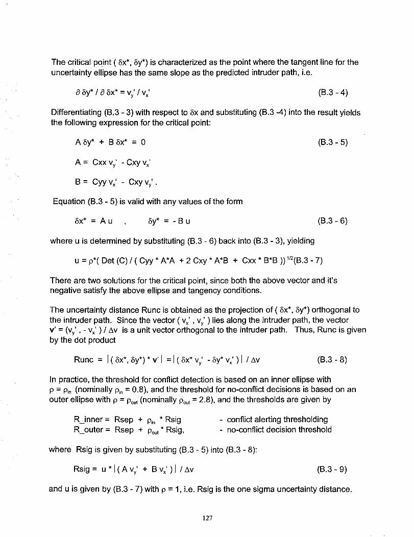
The critical point ( 5x*, 5y*) is characterized as the point where the tangent line for the
uncertainty ellipse has the same slope as the predicted intruder path, i.e.
a ,Sy*/ a 5x* = vy / Vx (B.3 -4)
Differentiating (B.3 - 3) with respect to 6x and substituting (B.3 -4) into the result yields
the following expression for the critical point:
A6y* + B6x* = 0 (B.3-5)
A= Cxxvy -Cxyvx
B= Cyyvx' - Cxyvy .
Equation (B.3 - 5) is valid with any values of the form
6x* = Au , 5y* = -Bu (B.3-6)
where u is determined by substituting (B.3 - 6) back into (B.3 - 3), yielding
u = p*( Det (C) / ( Cyy * A*A + 2 Cxy * A*B + Cxx * B*B )) 1_2(B.3- 7)
There are two solutions for the critical point, since both the above vector and it'snegative satisfy the above ellipse and tangency conditions.
The uncertainty distance Runc is obtained as the projection of ( 6x*, 5y*) orthogonal to
the intruder path. Since the vector ( Vx', Vy' ) lies along the intruder path, the vectorv' = (vy', - Vx' ) / Av is a unit vector orthogonal to the intruder path. Thus, Runc is givenby the dot product
Runc = l( 6x*, 6y*) * v'l = l( 6x* Vy' - 5y* Vx' )1 / Av (B.3 - 8)
In practice, the threshold for conflict detection is based on an inner ellipse with
P = Pin (nominally P_n= 0.8), and the threshold for no-conflict decisions is based on an
outer ellipse with p = Pout(nominally Pout= 2.8), and the thresholds are given by
R_inner = Rsep + P_n* Rsig
R_outer = Rsep + Pout* Rsig,
conflict alerting thresholding- no-conflict decision threshold
where Rsig is given by substituting (B.3 - 5) into (B.3 - 8):
Rsig= u*l(Avy + BVx )1 /Av (B.3-9)
and u is given by (B.3 - 7) with p = 1, i.e. Rsig is the one sigma uncertainty distance.
127

B.4 Predicted Loss-of-Separation Probability
One of the advantages of computing the predicted covariance matrix in (B.2-25) is that
collision risk analysis and probability calculations become feasible as by-products of the
conflict probe calculations, assuming that the intruder prediction errors (Sx, 5y) are
bivariate normal with zero means and covariance matrix C. The probability of a loss-
of-separation during a crossing encounter can be approximated by the probability that
the difference 5Cpa between the estimated and true CPA falls into the Loss-of-
Separation Region shown in Figure B-3. Since any point in the region described by
Rmin - Rsep <= 5Cpa <= Rmin + Rsep
will fall will within the ownship protected region at some time during a close encounter,
and the probability distribution of a deviation in 5Cpa is zero mean with standard
deviation Rsig, this implies that the probability of loss-of-separation Ps during an
encounter is approximately given by a one-dimensional normal distribution:
Ps = Prob(Gl<=N <=G2) = PN(G2)-PN(G1) (B.4- 1)
where N is a normal random variable with mean zero and unit variance, PN (X) denotes
the cumulative probability Prob ( N <= X ), and
G1 = ( Rmin - Rsep ) / Rsig (B.4- 2)
G2 = ( Rmin + Rsep) / Rsig.
Loss-of-
Separation
Region
Rmin - Rsep
One-Sigma
Uncertainty
Ellipse
At Tmin
Horizontal
Separation
Region
%
\
\
Intruder Path
Figure B-3: Geometry for Loss-of-Separation Probability
128

In practice, since the estimates of Cpa distance can vary significantly from one probe
update to the next, Rmin should be estimated using an average of Cpa estimates over
several probe updates. The probability function PNcan be easily computed using eitherpre-stored tabular values, or an analytic approximation.
B.5 Predicted Conflict Entry and Exit Times
Once a potential conflict has been detected, it is important to estimate the time until the
potential conflict begins, and the time until the potential conflict ends. Although weused a rough approximation for warning time in our Monte-Carlo studies, the equationused in Section A.6 may not be sufficiently accurate for medium term predictions in a
3-D conflict probe. In this section, we formulate the problem of estimating horizontalconflict entry and exit times, and show that the solution to this problem can be reduced
to that of solving a simple quadratic equation for an equivalent, transformed problem.
Conflict Entry and Exit Time Problem Formulation
Conceptually, a potential conflict begins when the intruder path uncertainty ellipse first
touches the ownship separation region, where the size of the uncertainty ellipse issufficiently large. See Figure B-4. The size of the uncertainty ellipse and the value of p
in (B.2-3) is determined such that the probability that prediction errors are contained
within the upper half plane bounded by the tangent line in Figure B-4 is close to 1.0.For example, we may require that the probability of the intruder falling in the lower half
plane be no greater than 1% at conflict entry time. The analysis in this case is similar tothat in Section B.4, i.e. the probability that the intruder lies below the tangent linereduces to that for a one-dimensional normal distribution. Choosing p such that PN (P)
= 0.99, ensures that no more than 1% of the prediction errors will fall in the lower half-plane. In this case, we obtain p = 2.33 which is an adequate upper bound on the size
of the uncertainty ellipse for determining conflict entry and exit times.
The conflict exit time is defined similarly, as the time when the separation circle and the
uncertainty ellipse just touch at the end of an encounter. The size of the uncertaintyellipse is the same as for conflict entry, since the probability requirement for conflict exitis the same, e.g. less than 1% probability that the intruder position will fall in the half-plane containing the ownship separation circle.
Problem Transformation and Solution for Entry and Exit Times
The problem of finding the points of tangency of the uncertainty ellipse and the ownship
separation circle, can be reduced to that of finding the intersection of the predicted
intruder path with an expanded ellipse centered at the origin, with semi-axis lengths;L1+ Rsep and ;L2+ Rsep, where ;L1 and ;L2 are the semi-axes of the uncertainty ellipse,
and the axes of the transformed ellipse are parallel to the uncertainty ellipse (Ref. 21, p.27). Figure B-5 shows the geometry of the transformed problem.
129

Non-Conflict 1Half- Plane
Tangent Line
9_2 /_ UncertaintyEllipse
_.1 At ConflictStart
Ownship
Horizontal
Separation JRegion Intruder Path
Figure B-4: Conflict Entry Time Geometry
Transformed Conflict
Ellipse for /---- Entry PointPotential /Conflict _ Conflict
/Exit Point
9_1+ Rsep /
Ownship
Horizontal
Separation
Region Intruder Path
Figure B-5: Equivalent Geometry for Conflict Entry and Exit Times
The calculation procedure for conflict entry and exit times consists of three steps:
130

Step 1: Find the orientation angle and semi-axes of the uncertainty ellipse
Suppose e denotes the orientation angle which diagonalizes the covariance matrixC(Tmin). Then the transformation of the covariance matrix from ownship coordinates to
principal axes diagonalizing the covariance matrix satisfies the matrix equation
i- (X1)2 0 -I = [-cos e sin 67 [- Cxx Cxy ] r-cos e -sin 0 -] (B.5 - 1)L 0 (;L2)q L-sin e cos eJ L Cxy cyy J L sin e cos eJ
Expanding the indicated matrix operations yields
(;L1)2 = Cxx*cos 20 + 2Cxy*cos0*sine +Cyy*sin 2e (B.5-2)
(X2)2 = Cxx * sin 2 0 2 Cxy * cos 19* sin e + Cyy * cos 2 e (B.5 - 3)
0 = Cxy*cos 2e - (Cxx-Cyy)*cose*sine - Cyy*sin 20 (B.5-4)
Solving (B.5 -4) for e yields
tan 2e = 2 Cxy / ( Cxx - Cyy ),
or equivalently,
e = arctan (2 Cxy / ( Cxx - Cyy ) ) / 2 (B.5 - 5)
The semi-axes ;L_and X2are obtained by taking the positive square roots of (B.5 -2),
and (B.5 - 3), respectively, where e is obtained from (B.5 -5).
Step 2: Find the covariance matrix of the transformed problem
Let D denote the covariance matrix of the transformed ellipse with orientation angle e
and semi-axes ;L_+ Rsep and ;L2 + Rsep. Then, the inverse transform to that in (B.5 -1)yields the transformed covariance matrix, i.e.
[- Dxx Dxy ] = [-cos e -sin e-] r- (;L_+Rsep) 2 0 -_[-cos e sin e -]
L Dxy DyyJ Lsin 0 cos eJL 0 (X2+Rsep)2_JL-sin e cos eJ
Expanding the above matrix equation yields the component equations
Dxx
Dxy
Dyy
= cos 2 e * (X_+Rsep) 2 + sin 2 e * (X2+Rsep) 2
= sin e *cos 0 *((;Ll+Rsep) 2 - (X2+Rsep) 2 )
= sin 2 e * (X_+Rsep) 2 + cos 2 e * (X2+Rsep) 2
(B.5 - 6)
131

Step 3: Solve for Conflict Entry and Exit Times T1 and T2
In the vicinity of Tmin we can ignore the wind shear terms and express the intruder pathin ownship coordinates using the approximate linear equation
FAx(t)-] = [-Ax'-] + At*[-Vx'-] (B.5-7)
L Ay(t) J L Ay'J L Vy'J ,
where At = t - Tmin, and the intruder position at Tmin is obtained by rotating (A.5 - 3)
by the ownship angle _o :
_-Ax' ] = [- cos Wo sin _o ] [- Ax(Tmin) ]
LAy' J L - sin _o cos _o J L Ay(Tmin) J .
The transformed uncertainty ellipse consists of all pairs ( Ax, Ay) such that
( Ax, Ay) [- Dxx Dxy -]-1 r Ax ] = 1 (B.5- 8)
LDxy gyyJ LAyJ
Expanding the indicated matrix operations yields the scalar equation
Dyy *Ax*Ax - 2 Dxy *Ax*Ay + Dxx *Ay*Ay = Det (D) (B.5 - 9)
where Det (D) = Dxx*Dyy - Dxy*Dxy. Substituting (B.5 - 7) above yields aquadratic equation for At. Combining similar terms in At yields
a'At 2 + 2b'At + c =0
where
a = Dyy * (v×')2 - 2 Dxy * Vx' * vy' + Dxx * (vy') 2
b = Dyy * Vx' * Ax' - 2 Dxy *(Ay' * Vx' + Ax' * vy') + Dxx * Ay' * vy'
c = Dyy * (Ax') 2 - 2 Dxy *Ax' *Ay' + Dxx * (Ay') 2 - det (D).
Consequently, solving the quadratic equation in (B.5 - 10) yields the followingexpressions for conflict entry and exit times:
T1 = Tmin-b/a -((b/a)2-c/a) 1/2
T2 = Tmin-b/a+((b/a)2-c/a) _/2
(B.5- 10)
(B.5- 11)
(B.5- 12)
(B.5- 13)
132
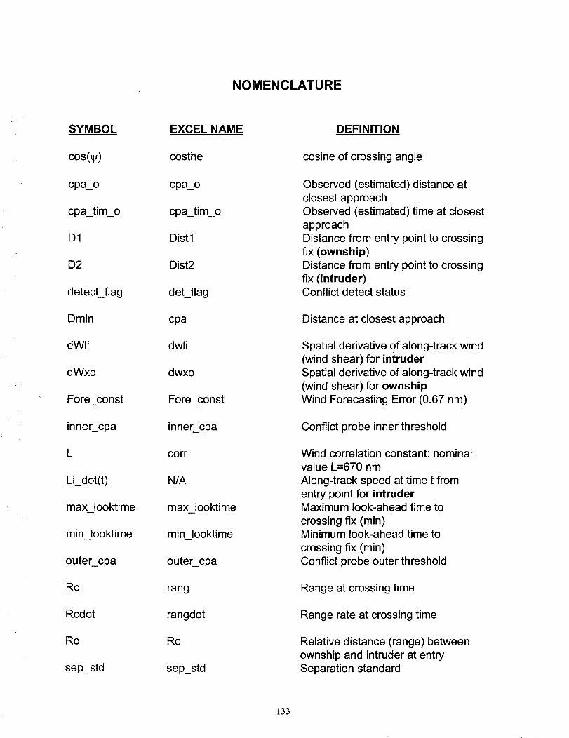
NOMENCLATURE
SYMBOL
cos(v)
cpa_o
cpa_tim_o
D1
D2
detect_flag
Dmin
dWli
dWxo
Fore constw
inner_cpa
L
LLdot(t)
max Iooktime
min Iooktime
outer_cpa
Rc
Rcdot
Ro
sep_std
EXCEL NAME
costhe
cpa_o
cpa_tim_o
Distl
Dist2
det_flag
cpa
dwli
dwxo
Fore const
inner_cpa
corr
N/A
max Iooktime
min Iooktime
outer_cpa
rang
rangdot
Ro
sep_std
DEFINITION
cosine of crossing angle
Observed (estimated) distance atclosest approach
Observed (estimated) time at closestapproach
Distance from entry point to crossingfix (ownship)Distance from entry point to crossing
fix (intruder)Conflict detect status
Distance at closest approach
Spatial derivative of along-track wind(wind shear) for intruderSpatial derivative of along-track wind
(wind shear) for ownshipWind Forecasting Error (0.67 nm)
Conflict probe inner threshold
Wind correlation constant: nominalvalue L=670 nm
Along-track speed at time t fromentry point for intruderMaximum look-ahead time to
crossing fix (min)Minimum look-ahead time to
crossing fix (min)Conflict probe outer threshold
Range at crossing time
Range rate at crossing time
Relative distance (range) betweenownship and intruder at entrySeparation standard
133

SYMBOL EXCEL NAME DEFINITION
sigy sigy Lateral conformance error
sin(w) sinthe sine of crossing angle
N/A Time
mc
Tmin
cross-time
cpa_tim
Mean time from entry to crossingfix
Time at closest approach
truth_flag truth_flag True cpa status
V1
V2
Wxc, Wyc
Wxi, Wyi
Wxo, Wyo
x_dot(t)
xldist
xldot
x2dist
x2dot
yldist
y2dist
y2dot
yoffl
yoff2
Vlbar
V2bar
WXC, WYC
WXl, WYI
WXO, WYO
N/A
xldist
xldot
x2dist
x2dot
yldist
y2dist
y2dot
yoffl
yoff2
Mean ground speed for ownshipincluding airspeed and mean wind
Mean ground speed for intruderincluding airspeed and mean windVector wind uncertainty at the
crossing fixVector wind uncertainty at the
entry point for intruderVector wind uncertainty at the entrypoint for ownship
Along-track speed at time t fromentry point for ownship
X coordinate distance at crossingtime (ownship)
X coordinate velocity at crossingtime (ownship)X coordinate distance at crossing
time (intruder)X coordinate velocity at crossing
time (intruder)Y coordinate distance at crossing
time (ownship)Y coordinate distance at crossingtime (intruder)
Y coordinate velocity at crossingtime (intruder) Note: yldot = 0.Lateral offset value for each Monte
Carlo run (ownship)Lateral offset value for each Monte
Carlo run (intruder)
134
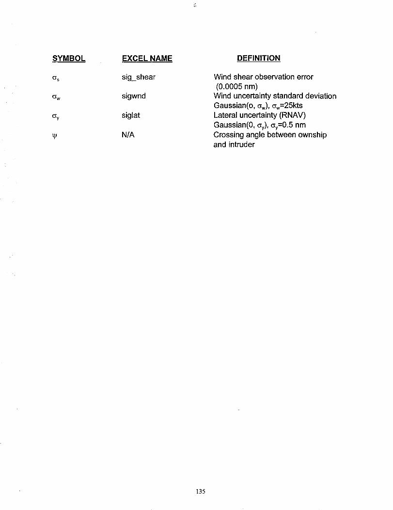
SYMBOL EXCEL NAME DEFINITION
(_'S sig_shear
sigwnd
siglat
N/A
Wind shear observation error
(0.0005 nm)
Wind uncertainty standard deviation
Gaussian(o, ew), _w =25kts
Lateral uncertainty (RNAV)
Gaussian(0, %), %=0.5 nm
Crossing angle between ownship
and intruder
135

REPORT DOCUMENTATION PAGEForm ApprovedOMB No, 0704-0188
Public reporting burden for this collectio¢l ot Ir_focmation is estknJted to average 1 hour per response, itt:duding the tJrna for reviewing _lstT1_tions, =matching existing data sources,
gathering and maintaining the ¢b_ nende¢l, and completing _ reviswtng the cdleoficn of Infocmation. Send comments regarding this burden estimate or any other aspect of this
¢o]icoficn of IofomwlJml, thduding suggestions for reducing this burden, to Washington He_rtel: Se_ Dire(orate for Information Operations and Repo.'l.s, 1215 Jefferson Davis
Highway, Sule 1204, Arlington, VA 22202-4302. and to the Off'ce of Management and Bucket, Paperwork Reduction Project (0704-0188), Wa_2dngton, DC 205_.
1. AGENCY USE ONLY (LemVe blank) 2. REPORT DATE
January 19974. TITLE AND SUBTITLE 5. FUNDING NUMBERS
Conflict Probe Concepts Analysis in Support of Free Right
G. AUTHOR(S)
Anthony W. Warren; Robert W. Schwab; Timothy J. Geels; and ArekShakarian
7. PERFORMINGORGANIZATIONNAME(S)ANDADDRESS(ES)
Boeing CommercialAirplane GroupSeattle, Washington 98124-2207
9. SPONSORING/MONITORINGAGENCYNAME(S)ANDADDRESS(ES)
National Aeronautics and Space AdministrationLangley Research CenterHampton, Virginia 23681-0001
3. REPORT TYPE AND DATES COVERED
Contractor Report
C NAS1-20267WU 538-04-14-01
8. PERFORMING ORGANIZATIONREPORT NUMBER
10. SPONSORING/MONITORINGAGENCY REPORT NUMBER
NASA CR-201623
11. SUPPLEMENTARY NOTES
langley Technical IVk)nitor. Sally C. Johnson
12a. DISTRIBUTION I AVAILABILITY STATEMENT
UNLIMITED - UNCLASSIFIED
SUBJECT CATEGORY: 04
12b. DISTRIBUTION CODE
_13. ABSTRACT (Ma_mum 200words)
This study develops an operational concept and requirements for en route Free Right using a simulation of the
Cleveland Air Route Traffic Control Center, and develops requirements for an automated conflict probe for use inthe Air Traffic Control (ATC) Centers. In this paper, we present the results of simulation studies and summarize
implementation concepts and infrastructure requirements to transition from the current air traffic control systemto mature Free Right. The transition path to Free Right envisioned in this paper assumes an orderlydevelopment of communications, navigation, and surveillance (CNS) technologies based on results from our
simulation studies. The main purpose of this study is to provide an overall context and methodology for
evaluating airborne and ground-based requirements for cooperative development of the future ATC system.
14.SUBJECTTERMS
Free RightAir Traffic Control
Air Traffic Management
17. SECURITY CLASSIRCATIONOF REPORT
UNCLASSIFIED
NSN 7540-01-280-5500
18. SECURITY CLASSIFICATIONOF THIS PAGE
UNCLASSIFIED
19. SECURITY CLASSIRCATIONOF ABSTRACT
UNCLASSIFIED
15. NUMBER OF PAGES
147
16. PRICE CODE
A07
20. UMITATION OF ABSTRACT
UNLIMITED
Standard Form 298 (Rev. 2-89)
Pralmribed by ANSI Std. Z39-18
298-102