Abstract

Image Analysis of 3D Cardiac Motion

Using Physical and Geometrical Models

Pengcheng Shi

1996

A novel approach has been developed to analyze the three-dimensional non-rigid motion

and deformation of the left ventricle of the heart from medical images. The hypothesis

is that a continuum biomechanical model based, integrated approach which allows in-

formation integration of multiple complementary imaging data can more accurately and

objectively quantify the motion and deformation of the left ventricle. This approach also

provides a natural framework to incorporate physical constraints related to known cardiac

parameters.

The left ventricle model is built upon continuum mechanics and is embedded in

a finite element framework, represented by a three-dimensional volumetric mesh. The

motion field on the myocardial boundaries is determined based on locating and matching

differential geometric features of the endocardial and epicardial surfaces. A mathematical

optimization strategy is used to combine a locally coherent smoothness model with data-

derived information. In addition, magnetic resonance phase contrast images provide

robust instantaneous velocity information within the myocardial wall. A finite element

framework and the governing equations of the system have been constructed, and the mid-

wall velocity and the boundary displacement vectors are used as data-based constraints

within the integration process. Displacement and strain measures are derived from the

solution of the system.

The algorithms have been implemented and applied to three-dimensional images

of normal and infarcted hearts. These algorithm-derived results are statistically compared

to implanted marker-derived measures for validation purposes.

Image Analysis of 3D Cardiac Motion

Using Physical and Geometrical Models

A Dissertation

Presented to the Faculty of the Graduate School

of

Yale University

in Candidacy for the Degree of

Doctor of Philosophy

by

Pengcheng Shi

Dissertation Director: James Scott Duncan

May 1996

c© 1997 by Pengcheng Shi

All Rights Reserved

Acknowledgment

I am grateful for the invaluable guidance and encouragement of my advisor, James Dun-

can. I am indebted to Lawrence Staib for his infinite patience and willingness to talk

about any subject at any time. I am thankful to Peter Schultheiss and David Kriegman

for serving on my committee and giving me helpful comments along the way. Thanks to

Dimitri Metaxas for serving as my external reader.

I must thank all the members of the Image Processing and Analysis Group at Yale:

Amir Amini, Ravi Bansal, Isil Bozma, Sudhakar Chelikani, Rupert Curwen, Gene Gindi,

Chuck Harrell, Mindy Lee, Francois Meyer, Wiro Neissen, Xenios Papademetris, Suguna

Pappu, N. Rajeevan, Anand Rangarajan, Hemant Tagare, Frans Vos, Yongmei Wang,

Marcel Worring, Lei Zhang, and George Zubal. I am particularly grateful to Glynn

Robinson for his help on visualization and liberalism, to Amit Chakraborty and John

McEachen for hanging tough together through the six years, and to Carolyn Meloling for

her numerous help.

I must also thank Albert Sinusas, Don Dione, and Eliot Heller for their help

regarding cardiac physiology. Special thanks to Todd Constable for the MR images, to

Erik Ritman for the DSR images, to Don Cox and Trey Crisco for help on continuum

mechanics and finite element method, and to John Holahan for help on statistical analysis.

I would like to thank my sister and my parents-in-law for their support and

encouragement. I will always be indebted to my parents. Without their moral and

intellectual guidance throughout my life, all these would be impossible.

I dedicate this thesis to my wife, Huifen, for her love and understanding.

iii

List of Figures

1.1 Overview of the system . . . . . . . . . . . . . . . . . . . . . . . . . . . . 6

3.1 LV boundary segmentation . . . . . . . . . . . . . . . . . . . . . . . . . . 26

3.2 Chamfer transformation templates . . . . . . . . . . . . . . . . . . . . . . 28

3.3 Shape based contour interpolation . . . . . . . . . . . . . . . . . . . . . . 30

3.4 Endocardial and epicardial contour stacks . . . . . . . . . . . . . . . . . . 31

3.5 Myocardial sample point set . . . . . . . . . . . . . . . . . . . . . . . . . . 33

3.6 Delaunay Tessellation and Voronoi diagram . . . . . . . . . . . . . . . . . 37

3.7 Computational flow of Delaunay triangulation . . . . . . . . . . . . . . . . 42

3.8 Two-dimensional Delaunay tessellation using incremental insertion method 43

3.9 Natural neighbor relationships . . . . . . . . . . . . . . . . . . . . . . . . 45

3.10 Natural neighbor local coordinates . . . . . . . . . . . . . . . . . . . . . . 51

3.11 Bounded Delaunay triangulation . . . . . . . . . . . . . . . . . . . . . . . 53

3.12 Mutual visibility criterion . . . . . . . . . . . . . . . . . . . . . . . . . . . 55

3.13 Constrained Delaunay tessellation . . . . . . . . . . . . . . . . . . . . . . 56

3.14 Two-dimensional Delaunay tessellation of myocardial slice . . . . . . . . . 60

3.15 Three-dimensional Delaunay tessellation of myocardium . . . . . . . . . . 62

3.16 Delaunay triangulation of myocardial surfaces . . . . . . . . . . . . . . . . 64

iv

4.1 Regular and non-shrinkage Gaussian smoothing of triangulated surface . . 70

4.2 Distance and natural weighted smoothing of uniformly sampled ellipsoidal

surface . . . . . . . . . . . . . . . . . . . . . . . . . . . . . . . . . . . . . . 73

4.3 Distance and natural weighted smoothing of non-uniformly sampled ellip-

soidal surface . . . . . . . . . . . . . . . . . . . . . . . . . . . . . . . . . . 74

4.4 Natural weighted non-shrinkage smoothing of myocardial surfaces . . . . . 75

4.5 A color spectrum representing the discrete surface types . . . . . . . . . . 84

4.6 Possible multiple mappings in the graph representation of surface patch . 88

4.7 Invalid neighborhood points . . . . . . . . . . . . . . . . . . . . . . . . . . 89

4.8 Shape maps of an endocardial surface derived from multi-scale graph func-

tions . . . . . . . . . . . . . . . . . . . . . . . . . . . . . . . . . . . . . . . 92

4.9 Shape maps of an epicardial surface derived from multi-scale graph functions 93

4.10 Potential energy and shape index maps of ellipsoidal surfaces . . . . . . . 95

4.11 Potential energy maps of an endocardial surface over the cardiac cycle . . 96

4.12 Potential energy maps of an epicardial surface over the cardiac cycle . . . 97

4.13 Trajectory of one endocardial point superimposed onto the potential energy

map of an endocardial surface from end diastole to end systole . . . . . . 102

4.14 Complete trajectory of one endocardial point over the cardiac cycle . . . . 103

4.15 Dense endocardial displacement vector field from ED to ES (MRI) . . . . 108

4.16 Bending energy maps between matched surfaces . . . . . . . . . . . . . . . 109

4.17 Bending energy maps of an endocardial surface over the cardiac cycle . . 110

4.18 Bending energy maps of an epicardial surface over the cardiac cycle . . . 111

4.19 MRI markers and their relative positions on the myocardium . . . . . . . 113

4.20 MRI image with endocardial and epicardial markers. . . . . . . . . . . . . 114

v

4.21 Sixteen spatial MRI images which cover the left ventricle . . . . . . . . . 116

4.22 Sixteen temporal MRI images of a mid-ventricle slice . . . . . . . . . . . . 117

4.23 Sixteen spatial DSR images which cover the left ventricle . . . . . . . . . 119

4.24 Sixteen temporal DSR images of a mid-ventricle slice . . . . . . . . . . . . 120

4.25 DSR images with endocardial and epicardial markers . . . . . . . . . . . . 121

4.26 Dense endocardial displacement vector field from ED to ES (DSR) . . . . 122

4.27 Visual comparison of algorithm-derived and implanted marker trajectories

(MRI study) . . . . . . . . . . . . . . . . . . . . . . . . . . . . . . . . . . 131

4.28 Visual comparison of algorithm-derived and implanted marker trajectories

(DSR study) . . . . . . . . . . . . . . . . . . . . . . . . . . . . . . . . . . 132

4.29 Baseline and post-infarct endocardial path length maps . . . . . . . . . . 135

4.30 Change in endocardial path length from baseline to post-infarct condition 136

4.31 Post Mortem injury from TTC staining . . . . . . . . . . . . . . . . . . . 139

4.32 Myocardial injury zone from SPECT counts . . . . . . . . . . . . . . . . . 141

5.1 Phase contrast MR images . . . . . . . . . . . . . . . . . . . . . . . . . . . 149

5.2 3D MR phase contrast images . . . . . . . . . . . . . . . . . . . . . . . . . 188

5.3 Myocardial surfaces derived from phase contrast MR images . . . . . . . . 189

5.4 Volumetric finite element mesh of the mid-ventricle from phase contrast

MR images . . . . . . . . . . . . . . . . . . . . . . . . . . . . . . . . . . . 191

5.5 Dense field displacement vector map (2D projection) from the integrated

framework . . . . . . . . . . . . . . . . . . . . . . . . . . . . . . . . . . . . 192

5.6 3D strain maps of mid-ventricle (ED-ES) . . . . . . . . . . . . . . . . . . 194

5.7 3D principal strain maps of mid-ventricle (ED-ES) . . . . . . . . . . . . . 195

vi

5.8 Temporal maps of the first principal strain (ED-ES) from phase contrast

MR images . . . . . . . . . . . . . . . . . . . . . . . . . . . . . . . . . . . 197

A.1 Compute the landmark net expanding-shrinking force in the feedback mech-

anism . . . . . . . . . . . . . . . . . . . . . . . . . . . . . . . . . . . . . . 205

A.2 Effect of the feedback mechanism . . . . . . . . . . . . . . . . . . . . . . . 206

vii

List of Tables

4.1 Comparison of distance and natural weighted smoothing . . . . . . . . . . 72

4.2 Discrete surface classification using shape index function . . . . . . . . . . 83

4.3 Average positional errors between implanted markers and algorithm-derived

point positions . . . . . . . . . . . . . . . . . . . . . . . . . . . . . . . . . 123

4.4 Positional errors between endocardial markers and algorithm-derived point

positions for each canine MRI studies observed under baseline condition . 125

4.5 Positional errors between epicardial markers and algorithm-derived point

positions for each canine MRI studies observed under baseline condition . 126

4.6 Positional errors between endocardial markers and algorithm-derived point

positions for each canine MRI studies observed under post-infarct condition127

4.7 Positional errors between epicardial markers and algorithm-derived point

positions for each canine MRI studies observed under post-infarct condition128

4.8 Positional errors between endocardial markers and algorithm-derived point

positions for each canine DSR studies observed under baseline condition . 129

4.9 Positional errors between epicardial markers and algorithm-derived point

positions for each canine DSR studies observed under baseline condition . 130

4.10 Average positional errors over time. . . . . . . . . . . . . . . . . . . . . . 133

viii

4.11 Path length measure observed in the infarct and normal zones under base-

line and post-infarct conditions . . . . . . . . . . . . . . . . . . . . . . . . 137

4.12 Correlation between post mortem and in vivo infarct areas. . . . . . . . . 140

4.13 Wall thickening measure observed in the infarct and normal zones under

baseline and post-infarct conditions . . . . . . . . . . . . . . . . . . . . . . 142

ix

Contents

Acknowledgements iii

List of Figures iv

List of Tables viii

1 Introduction 1

1.1 Introduction to the Problem . . . . . . . . . . . . . . . . . . . . . . . . . . 3

1.2 Overview of the Framework . . . . . . . . . . . . . . . . . . . . . . . . . . 4

1.3 Contributions . . . . . . . . . . . . . . . . . . . . . . . . . . . . . . . . . . 5

2 Background and Related Work 8

2.1 Medical Imaging Based LV Analysis . . . . . . . . . . . . . . . . . . . . . 9

2.1.1 Image Analysis Approaches . . . . . . . . . . . . . . . . . . . . . . 9

2.1.2 Imaging Physics Based Approach . . . . . . . . . . . . . . . . . . . 12

2.1.2.1 Magnetic Resonance Tagging . . . . . . . . . . . . . . . . 12

2.1.2.2 Magnetic Resonance Phase Contrast . . . . . . . . . . . . 16

2.2 Computer Vision Based Motion Analysis . . . . . . . . . . . . . . . . . . . 18

2.3 Biomechanical Models and Myocardial Deformation Analysis . . . . . . . 20

x

3 Geometrical Representation 23

3.1 Introduction . . . . . . . . . . . . . . . . . . . . . . . . . . . . . . . . . . . 23

3.2 Object Segmentation . . . . . . . . . . . . . . . . . . . . . . . . . . . . . . 24

3.2.1 Boundary Segmentation . . . . . . . . . . . . . . . . . . . . . . . . 25

3.2.2 Shape-Based Interpolation of Contours . . . . . . . . . . . . . . . . 27

3.2.3 Mid-Wall Sample Points . . . . . . . . . . . . . . . . . . . . . . . . 29

3.3 Delaunay Tessellation . . . . . . . . . . . . . . . . . . . . . . . . . . . . . 32

3.3.1 Assumptions and Definitions . . . . . . . . . . . . . . . . . . . . . 32

3.3.2 Properties . . . . . . . . . . . . . . . . . . . . . . . . . . . . . . . . 38

3.3.3 Construction . . . . . . . . . . . . . . . . . . . . . . . . . . . . . . 40

3.3.4 Natural Neighbor Relationship . . . . . . . . . . . . . . . . . . . . 44

3.3.4.1 k-order Natural Neighbor Relationship . . . . . . . . . . 44

3.3.4.2 Multi-Order Natural Neighbor Smoothing and Interpolation 46

3.3.4.3 Natural Weighted Smoothing and Interpolation . . . . . . 47

3.4 Modified Delaunay Tessellation . . . . . . . . . . . . . . . . . . . . . . . . 50

3.4.1 Bounded Delaunay Tessellation . . . . . . . . . . . . . . . . . . . . 52

3.4.2 Constrained Delaunay Tessellation . . . . . . . . . . . . . . . . . . 54

3.5 Delaunay Tessellation of Left Ventricle . . . . . . . . . . . . . . . . . . . . 57

3.5.1 Two Dimensional LV Tessellation . . . . . . . . . . . . . . . . . . . 58

3.5.2 Three Dimensional LV Tessellation . . . . . . . . . . . . . . . . . . 59

3.6 Conclusion . . . . . . . . . . . . . . . . . . . . . . . . . . . . . . . . . . . 63

4 Boundary Motion Analysis 65

4.1 Introduction . . . . . . . . . . . . . . . . . . . . . . . . . . . . . . . . . . . 65

4.2 Triangulated Surface Smoothing . . . . . . . . . . . . . . . . . . . . . . . 66

xi

4.3 Shape Characterization . . . . . . . . . . . . . . . . . . . . . . . . . . . . 76

4.3.1 Differential Geometry of Surface . . . . . . . . . . . . . . . . . . . 76

4.3.2 Shape Characterization of Triangulated Surfaces . . . . . . . . . . 84

4.3.2.1 Local Surface in Graph Form . . . . . . . . . . . . . . . . 84

4.3.2.2 Multi-Order Local Surface Fitting . . . . . . . . . . . . . 86

4.4 Surface Motion Field . . . . . . . . . . . . . . . . . . . . . . . . . . . . . . 91

4.4.1 Thin Plate Bending Model . . . . . . . . . . . . . . . . . . . . . . 94

4.4.2 Initial Surface Point Match . . . . . . . . . . . . . . . . . . . . . . 99

4.4.3 Optimal Dense Motion Field . . . . . . . . . . . . . . . . . . . . . 104

4.5 Experiments . . . . . . . . . . . . . . . . . . . . . . . . . . . . . . . . . . . 107

4.5.1 Magnetic Resonance Imaging Data . . . . . . . . . . . . . . . . . . 112

4.5.2 Dynamic Spatial Reconstructor Data . . . . . . . . . . . . . . . . . 115

4.5.3 Motion Validation . . . . . . . . . . . . . . . . . . . . . . . . . . . 118

4.5.4 Injury Validation . . . . . . . . . . . . . . . . . . . . . . . . . . . . 130

4.5.4.1 Path Length . . . . . . . . . . . . . . . . . . . . . . . . . 133

4.5.4.2 Wall Thickening . . . . . . . . . . . . . . . . . . . . . . . 140

4.6 Conclusion . . . . . . . . . . . . . . . . . . . . . . . . . . . . . . . . . . . 143

5 Volumetric Deformation Analysis 144

5.1 Introduction . . . . . . . . . . . . . . . . . . . . . . . . . . . . . . . . . . . 144

5.2 Image-Derived Information . . . . . . . . . . . . . . . . . . . . . . . . . . 145

5.2.1 Shape-Based Boundary Displacement . . . . . . . . . . . . . . . . 146

5.2.2 MR Phase Contrast Images and Mid-Wall Instantaneous Velocity . 146

5.2.3 Other Image-Derived Data . . . . . . . . . . . . . . . . . . . . . . 150

5.2.3.1 MR Tagging and Tag Displacement . . . . . . . . . . . . 150

xii

5.2.3.2 DSR Image and Optical Flow . . . . . . . . . . . . . . . . 151

5.2.3.3 Echocardiography and Doppler Velocity . . . . . . . . . . 151

5.3 Continuum Mechanical Models . . . . . . . . . . . . . . . . . . . . . . . . 152

5.3.1 Continuum Mechanics . . . . . . . . . . . . . . . . . . . . . . . . . 152

5.3.1.1 Deformation Measure . . . . . . . . . . . . . . . . . . . . 153

5.3.1.2 Constitutive Equation . . . . . . . . . . . . . . . . . . . . 155

5.3.2 Models of the Myocardium . . . . . . . . . . . . . . . . . . . . . . 157

5.4 Finite Element Analysis . . . . . . . . . . . . . . . . . . . . . . . . . . . . 163

5.4.1 Element and Interpolation Function . . . . . . . . . . . . . . . . . 164

5.4.2 Finite Element Formulation . . . . . . . . . . . . . . . . . . . . . . 166

5.4.2.1 Minimum Potential Energy Principle . . . . . . . . . . . 167

5.4.2.2 Element Formulation . . . . . . . . . . . . . . . . . . . . 168

5.4.2.3 System Formulation . . . . . . . . . . . . . . . . . . . . . 174

5.5 Integrated Motion/Deformation Analysis . . . . . . . . . . . . . . . . . . . 176

5.5.1 Initial Conditions . . . . . . . . . . . . . . . . . . . . . . . . . . . . 177

5.5.2 Boundary Conditions . . . . . . . . . . . . . . . . . . . . . . . . . 179

5.5.3 Numerical Solution . . . . . . . . . . . . . . . . . . . . . . . . . . . 181

5.6 Experiments . . . . . . . . . . . . . . . . . . . . . . . . . . . . . . . . . . . 187

5.7 Conclusion . . . . . . . . . . . . . . . . . . . . . . . . . . . . . . . . . . . 198

6 Summary 200

Appendix 202

A 2D Feedback Mechanism 202

Bibliography 207

xiii

Chapter 1

Introduction

A computer vision system analyzes an image or sequence of images and produces descrip-

tions of objects that are imaged. Recovery of motion and deformation information from

pictorial data is an important part of many vision systems. The goal is to extract quan-

titatively the temporal changes, rigid or non-rigid, of the objects depicted in the image

sequence. Motion recovery in general is a correspondence problem, which involves finding

the positions of the object points at successive image frames (the motion of each point),

as well as measuring the motion difference among different object points (the deformation

of the object) if non-rigid motion is presented in the image sequence. For cardiac mo-

tion, which is the focus of this thesis, the heart moves and deforms in three-dimensional

space. Hence, the goal of our image analysis system is to depict the non-rigid motion

characteristics of the heart from three-dimensional image sequences.

The intensity and texture variations of the image sequence provide initial visual

cues of the changes of the object. However, as Horn suggested, a motion field, the

displacement vector field of each point of the object in the image, is usually not exactly the

same as the optical flow, the apparent motion of the brightness pattern[52]. Furthermore,

1

2

it has been demonstrated that the actual correspondence process takes place beyond the

level of the raw gray level intensity values[70]. It has been suggested in Ullman’s report

that, at least in the human visual system, the edges or the boundaries of the objects are

the tokens used in the correspondence process[130].

In the analysis of cardiac motion, characteristics of the boundary shape of the

left ventricle have been used as the tracking tokens over the temporal sequence. One

important recent study that attempts to track cardiac point trajectories using visually

extracted shape landmarks is that of Slager[120]. The results of this two-dimensional

effort have been carefully validated using implanted markers, with the correlation between

the movement of shape landmarks and implanted markers found to be 0.86. At least for

cardiac motion, provided that the temporal sampling of the image sequence is not too

long in relation to the velocities of the motion, it is not hard to see that the closer

and more similar two boundary features are in the successive frames, the more likely

they are to correspond to each other. The challenge then becomes how to define this

similarity which is both visually and physically meaningful for the matching process.

Local shape properties of the boundary provide powerful matching cues, especially for

differential geometric landmarks, such as corners. However, the correspondence process

involves more than finding purely local minima of the similarity function. A mathematical

optimization strategy is needed to combine the similarity information with the effects of

various kinds of other local competition to determine the final mapping[3, 114, 116].

With the new progress in magnetic resonance imaging, dense instantaneous ve-

locity maps of the moving heart become available, in addition to traditional anatomical

images. In principle, the integration of the velocity map yields the estimated positions of

the object points at the next time frame. In practice, however, serious numerical difficul-

3

ties can arise because of the temporal sampling rate and the noise in the imaging process.

Nonetheless, the instantaneous velocity map can help solve the correspondence problem,

if not alone, in conjunction with other matching cues.

The integration of multiple image-derived information should only take place in

frameworks which account for the strength and weakness of each data source. This could

be done either through a statistical model using a maximum a posteriori framework, or

through a physical model using the minimum potential energy approach upon which this

thesis is based. For the physics-based framework, the constraints should be based on the

geometric and physical models of the object and the statistical models of the temporal

changes. Continuum mechanical models and finite element analysis provide a reasonable

framework to accomplish this task.

1.1 Introduction to the Problem

Motion and deformation analysis is of great interest in many image understanding and

computer vision applications including biomedical image analysis, robot vision, and pat-

tern recognition. It plays an especially essential role in computer vision research areas

which analyze natural objects, such as facial identification and recognition, articulated

motion analysis, satellite weather map analysis, and cardiac function analysis, which is

the focus of this thesis.

The measurement of regional myocardial injury due to ischemic heart disease

is an important clinical problem. Accurate estimates of heart motion and deformation

are essential to evaluate normal and abnormal cardiac physiology and mechanics. It is

the goal of many forms of cardiac imaging and image analysis methods to measure the

regional function of the left ventricle (LV) in an effort to isolate the location, severity, and

4

extent of ischemic or infarcted myocardium. The complexity of the LV non-rigid motion

and the lack of reference landmarks within the myocardium imply that the true motion

trajectories of tissue elements are, at best, difficult to infer from sequential images.

This thesis presents a novel approach of estimating left ventricular motion and

deformation by integrating instantaneous velocity information obtained within the mid-

wall region with shape-based displacement information found on the boundaries of the

left ventricle. The framework is based on continuum mechanical constraints of the my-

ocardium, and is numerically solved using finite element method.

1.2 Overview of the Framework

A complete system using geometric and physical models for recovering motion and defor-

mation of the left ventricle from image sequences has been developed. The approach is

composed of three main elements: the geometric representation of the left ventricle, the

modeling and motion tracking of the boundary surfaces, and the integration of comple-

mentary information using continuum mechanical models and finite element analysis. In

Chapter 3, the geometrical representation of the left ventricle is constructed by surface and

volumetric Delaunay tessellation. In Chapter 4, the myocardial surface points are charac-

terized by their local differential geometrical properties, computed in a multi-scale fashion

based on the multi-order natural neighbor relationship. The boundary matching measure

is based on an ideal thin plate model of a local surface patch and a minimum bending

energy criterion. Combined with local smoothness constraints, the boundary matching

process yields a set of optimal matched displacement vectors, Uboundary(ti, ti+1), between

pairs of image frames. In Chapter 5, the need for, and examples of the biomechanical

models to help solve the inverse recovery problem are discussed, and a finite element

5

integration framework is developed. The governing equations of the system are derived,

based on the minimum potential energy principle. The boundary displacement informa-

tion and the mid-wall velocity constraints Umidwall(ti) from phase contrast images are

used as the boundary and initial conditions of the framework. Numerical solution to the

governing equations gives the motion and deformation descriptions of the left ventricle.

A diagram outlining the system is shown in Figure 1.1.

1.3 Contributions

A novel approach has been developed to analyze three dimensional non-rigid motion and

deformation of the left ventricle of the heart from medical images. It is a new physically

modeled dynamic system which combines physical information of the left ventricle with

multiple, complementary sources of imaging data to depict the temporal motion and

deformation information. The algorithms are implemented and applied to real medical

images of normal and infarcted canine hearts.

We developed a new, shape-based strategy to track myocardial boundary motion

in three dimensions based on matching multi-scale geometric features and a local smooth-

ness model. We have proposed the first volumetric continuum mechanical model-based

approach to analyze the temporal dynamics of moving objects from imaging data. And we

have constructed the first finite element framework to integrate complementary bound-

ary displacement and mid-wall instantaneous velocity information to recover motion and

deformation of the left ventricle.

We have exploited the attractive new research direction of using continuum me-

chanical models as a means to guide dynamic information analysis from complementary

imaging data. The approach provides a natural framework to integrate physical informa-

6

Contour Interpolation

Contour Stacks

Delaunay Tessellation

Surface MeshVolume Mesh

MotionInformationFrom ImagingPhysics(acceleration)(velocity)(displacement)

IMAGE

Segmentation

ShapeCharacteristics

SurfaceDisplacement

FiniteElementMotionAnalysis

ContinuumMechanicalModels

Motion/Deformation Descriptions

Figure 1.1: Overview of the system.

7

tion of an object with visual image constraints. This model-based, integrated strategy

should allow us to obtain more robust descriptions of motion and deformation of the

myocardial wall.

Chapter 2

Background and Related Work

Ischemic heart disease is a major clinical problem. Accurate estimation of heart motion

and deformation is essential to evaluate normal and abnormal cardiac physiology and

mechanics. It is the fundamental goal of many efforts of cardiac imaging and image anal-

ysis to measure the regional function of the left ventricle (LV), through LV wall motion,

thickening, and strain measurements, in an effort to isolate the location, severity, and ex-

tent of ischemic or infarcted myocardium. It is also felt that image-based serial analysis

of regional function is helpful in assessing myocardial salvage to determine the efficacy of

therapeutic agents and/or angioplasty (e.g. [22, 43]), and has important implications for

understanding the pathophysiology of the remodeling process, especially issues related to

the extent of injury.

Motion and deformation analysis is also of great interest in general computer

vision research and application. Motion recovery plays an essential role in analyzing the

dynamic behavior of natural objects. The goal is to depict the temporal changes of objects

from sequential images, and the results are usually represented by dense trajectory fields

or correspondence maps. The non-medical applications include robot navigation[34],

8

9

facial recognition[15, 32], articulated motion[42, 83], satellite weather map analysis[93],

etc.

There have been considerable efforts within the medical image analysis and com-

puter vision communities aimed at trying to find sparse correspondences and then map

one object into another at the next time instant, which is an important underlying aspect

of many motion measurement approaches. In addition, a significant level of activity has

been performed within the magnetic resonance imaging (MRI) community regarding the

measurement of LV motion and strain using MR tagging, and to a lesser extent, MR

phase velocity measurements. Some very active research in the biomechanics commu-

nity aimed at deriving local LV deformation information and constitutive relationships

experimentally is also invaluable to be incorporated into image analysis based efforts.

2.1 Medical Imaging Based LV Analysis

In the cardiac imaging and image analysis community, there have been a number of

approaches aimed at addressing the problem of quantifying LV function using image

data, most often related to quantifying parameters related to either myocardial boundary

motion or LV thickening from 2D image sequence data, and rarely focused on trying to

fully characterize transmural function. Out of plane motion, and twisting or torsional

motion are typically ignored. Recently, new progress in imaging physics, such as MR

tagging and phase contrast MR, has provided new directions in analyzing the true 3D

motion of the LV.

10

2.1.1 Image Analysis Approaches

In the medical image analysis community, earlier approaches to measuring cardiac motion

fall into two different groups. The first group attempts to measure LV function and

motion by detecting grey level changes over time for each pixel. Included in this school

are techniques which compute phase changes across the temporal dimension[68], find

regional ejection fractions between end-systole (ES) and end-diastole (ED) in a set of

radial sections extending from the centroid of the ventricle[6], etc. Many efforts have

tried to compute the optical flow under different assumptions and conditions, including

work by Mailloux[69], Song[122], and Tistarelli[128]. For these work, assumptions about

the object and its motion fields are needed to obtain a unique solution. In addition to the

fact that optical flow is usually not the same as the motion field of the physical material

points[52], it is quite difficult to post-process the optical flow to separate the LV wall

from any other motion in the image for diagnostic purposes.

The second type of approach tracks the motion of the pre-extracted boundaries,

contours in 2D and surfaces in 3D, of the cardiac wall. The task is to estimate the

motion of boundary points between frames and is performed using geometric measures.

The algorithms include the chord shortening method by Gelberg[39], which depends on

accurately locating a reference point or line, and the centerline method by Bolson[17],

which measures the thickness of the region between the ED and ES contours. This

latter method essentially treats the measurement of the ED-ES contour difference as a

thickness that must be quantified, ignoring the more fundamental goal of motion analysis

of tracking the trajectory of each point of the LV wall through the cardiac cycle. One

important study by Slager[120] attempts to use contour shape landmarks to track point

motion over time from two-dimensional image sequence, and validates the results using

11

implanted markers. The correlation between the motion of visually extracted shape

landmarks and the implanted marker movement is 0.86, which seems to support the

concept of tracking identifiable shape cues over time. More recently, several researchers

have been pursuing boundary shape matching ideas. Goldgof used Gaussian curvature

under a conformal stretching model[63], Amini and Duncan developed a hybrid bending

and stretching model[3], McEachen and Duncan used an elastic rod bending model[61,

92], to track LV motion. Another effort of interest is that of Bookstein’s[18]. It used

morphometrics for measuring shape change to effectively interpolate motion in regions

between the landmarks for cases where these corresponding landmarks are already clearly

distinguished.

The issue of tracking object points over a multi-frame temporal sequence has

often been avoided in cardiac image analysis. Many of the LV motion quantification

approaches(e.g.[17, 39, 144]) use only the ED and ES image frames. However, the heart

actually goes through a temporal wave of contraction, twisting and expansion, and the

asynchrony of LV motion and deformation from time to time, as well as from region to

region, may be indicative of the state of health. This asynchrony has been shown to

be very important in studying coronary artery disease[40]. Unfortunately, even several

attempts that do aim at motion measurement over the entire cardiac cycle, including some

early work on characteristics of LV contraction[23, 47] and work using nuclear medicine

images[6], are limited by the need to set up a reference system that measures motion as

if it were emanating radially from a single point[112].

Many methods[6, 17, 23, 39, 61, 92, 120, 144] have been hampered in making

accurate and reliable quantitative regional LV function measurements due to the fact that

the heart is a non-rigid moving object that rotates, translates, and deforms in 3D space,

12

whereas these approaches rely on 2D image sequence data (either projections of a 3D

object onto fixed 2D planes, or 2D sections). Motion and thickening measurements from

2D image sequences most likely are not made from the same points on the LV boundaries

at different time instants, and hence do not track the true movement of the heart. Work

in the general area of 3D quantitative analysis of cardiac motion has been relatively

minimal[33, 105, 104]. In addition to the few 3D optical flow based[122] and surface

based[3, 63] methods mentioned above, Baker’s weaving-wall-surface-building approach

uses Laplacian zero crossings as the features upon which motion tracking is based[10].

One difficulty with this method is that a reference path for motion finding must be known

beforehand.

The study of volumetric LV motion and deformation has been almost nonexistent,

although the progress in imaging physics has made it a more attackable problem[24, 28,

142]. However, volumetric analysis for classification of myocardial infarction into trans-

mural or non-transmural injury is valuable and has interested many investigators for more

than 30 years. The transmural extent of myocardial injury has important implications

regarding infarct expansion[31], aneurysm formation[45], LV remodeling[101], myocardial

denervation[27] and most importantly, patient survival[31]. The in vivo characterization

of 3D transmural strain from non-invasive image data should be helpful for determining

the transmurality of injury. Measures of strain have been shown to be useful clinically

(e.g. [14]) as well as for basic understanding of biomechanical properties of the heart[58].

13

2.1.2 Imaging Physics Based Approach

2.1.2.1 Magnetic Resonance Tagging

In magnetic resonance tagging, a spatially varying pattern of magnetization is encoded

into the myocardium prior to each phase-encoded data acquisition cycle of a spin-echo

imaging sequence, forming a grid pattern of image voids generated at each time instant

in the cardiac cycle[8, 143]. Motion occurring between the tag pulse sequence and the

image pulse sequence results in a distortion of the tag pattern, and their deformation

can be tracked over a portion of the cycle, primarily using gated acquisition techniques.

Much of the current efforts (such as those of Axel[8] and Zerhouni[143]) on using the

grid tagging approach to the measurement of myocardial motion and deformation are

focused on how to create dense fields of measurements in 3D by putting together several

orthogonal tagging grid acquisitions. The motion and deformation descriptions are then

derived from the sparse set of tag-tag or tag-boundary crossings.

The MR tagging based approaches certainly show promise but still have some

major limitations. It remains a fundamental issue to track the tags over the complete LV

cycle due to decay of the tags with time, which is often remedied by performing a second

acquisition (a re-tagging) somewhere later in the cardiac cycle. In general, the same tissue

elements are not tagged in each of the two tagging processes, hence the motion trajectory

of the tag crossing point in each tagging sequence is not for the same tissue or point. This

issue, plus the fact that the grid spacings are often quite far apart (on the order of 7mm

spacings and 2-5mm thick tags for the SPAMM tagging[139] and even further apart at

the epicardium for the radial Star-burst tagging[143]), means that the interpolated dense

displacement fields from two tagging processes may well be incoherent between each other.

In addition to the common practice of hand picking tag crossing points, algorithms to

14

segment the tag lines and detect the tag crossings over time have been mainly based on

deformable snake and tag profile models[2, 46, 113, 141] with modest success.

It is still quite difficult to obtain acquisitions and assemble the detected tags for

a robust 3D analysis. One can only obtain sparse in-plane motion, the approximated

2D projection of the 3D motion of the material points being imaged, from tagging im-

age sequence[94]. In order to obtain data pertaining to deformation in three dimensions,

2D tag data must be acquired in two orthogonal views, typically short axis and long

axis[9]. Once again, the same tissue elements are not tagged in each of the two views,

and thus the deformation in each view must be seen as partial 2D data at different

points that contributes to an overall scheme aimed at estimating the complete 3D motion

and deformation. A variety of approaches have been designed to attack this interpola-

tion/estimation problem, with each approach making certain assumptions. Several of the

most interesting ideas are the use of finite element models using spring-like interconnec-

tions and nonlinear basis functions by Young and Axel[139], the use of locally deformable

superquadrics by Metaxas and Park[95, 94], the use of stochastic models and statistical

estimation techniques by Denney and Prince[28], and the use of B-snake grid by Amini[2].

In [139], a finite element grid is fitted to the corresponded SPAMM tag crossing

displacements in order to interpolate between the sparse actual data points. The grid it-

self has a fairly small number of nodes however, and results in a fairly gross interpolation,

although the errors computed in the simulations are reasonable. The goal of the work was

to compute the mid-ventricular strain present in the LV, and the paper includes a smooth

surface visualization of the interpolated strains. This effort is related to our approach

in using finite element based framework, although key differences are in the density and

formation of the 3D grid (a uniformly dense transmural grid versus sparse endocardial

15

and epicardial meshes with linear interpolation to fill in transmurally), and the phys-

ical models used (a continuum mechanics model versus a spring-like connected mesh).

More recently, there has been new work moving toward the use of locally deformable

superquadrics[95, 94] as a parameterized model that can be used as the framework for

assembling MR tag data. This provides an interesting and possibly robust basis upon

which to assemble tag information, and the global motion parameters of interest can be

extracted. All of these efforts have typically proceeded using MR tag data in the mid-

wall, and extrapolating constraints to the endocardial and epicardial surfaces through

the constructed finite element grid, although simple boundary constraints (closest point

correspondence) are used in the latter approach[94]. However, due to the sparse x − y

grid nature of the SPAMM tags, the only truly reliable, corresponded tag-crossing dis-

placement information will come from the mid-wall tag sites. This means that at any

one time instant, point-based LV function measures such as strain will be quite accurate

in the mid-LV wall region, but will tend to be noisy and inaccurate near the endocardial

and epicardial boundaries, as the grids cross over into the LV blood pool or the pericar-

dial space. We note that the authors claim that useful information is also available from

the tag lines, not just the crossings. However, MR tagging itself does not provides the

correspondences of the non-crossing tag line points, they needed to be computed from

image analysis algorithms.

Several other efforts aimed at assembling 3D maps of myocardial deformation use

the Star-burst radial MR tagging scheme, which provides accurate displacement informa-

tion at the vary sparse tag-boundary crossing points, typically sixteen points per slice.

In [85], a special MR acquisition sequence is used to obtain 3D tag information one com-

ponent at a time, again generating a sparse set of corresponded tag points. Then, a high

16

order polynomial is fitted to the displacement field in order to interpolate between the

sparse data points. Alternatively, an estimation theory based idea has been proposed to

use a stochastic vector field to assist in the interpolation[28]. This approach uses fairly

weak assumptions on the specifics of heart wall motion as compared to some of the other

techniques mentioned above, and the Fisher estimate that is used in the approach can

help relating estimation accuracy to the number of tag lines needed. On the down side,

however, this approach actually increases the errors at the boundaries of the myocardium,

according to the phantom studies.

While some of the approaches described above are related to and can be used by

our continuum model-based approach, these ideas are geared toward dealing exclusively

with different types of MR tagging data, and provide trustworthy results only at mid-wall

(SPAMM) or boundary (Star-burst). Also, while there is no doubt that MR tagging po-

tentially provides unique and interesting data regarding LV myocardial movement, there

are quite a few processing steps required to assemble the data into meaningful measures

of 3D deformation even after the acquisition. Just having the MR tag data available

does not alone mean that physiologically and clinically accurate analyses are forthcom-

ing. The proper choice of image analysis and processing algorithms for assembling these

data remains a significant open question.

2.1.2.2 Magnetic Resonance Phase Contrast

Another new approach for motion tracking is the use of phase contrast MR imaging.

Changes in magnetic resonance phase signal due to motion of tissue within a fixed voxel

or volume of interest are used to assist in estimating instantaneous, localized velocities,

and ultimately cardiac motion and deformation throughout the cardiac cycle[24, 81, 99,

96, 98, 97].

17

The magnetic resonance phase contrast velocity technique relies on the fact that

a uniform motion of tissue in the presence of a magnetic field gradient produces a change

in the MR signal phase that is proportional to its velocity. The velocity in a particular

spatial direction can be estimated by measuring the difference in phase shift between two

acquisitions with different first gradient moments. Velocity maps encoded for motion in

three spatial dimensions may easily be obtained at multiple time instances throughout the

cardiac cycle using a phase contrast cine-MR imaging sequence. The acquired velocity

maps may then be used to provide information on tissue displacement, strain, strain

rate, and other quantitative measures of deformation. In principle, these instantaneous

velocities can be derived for each pixel in an image acquisition. However, currently phase

contrast velocity estimates near the endocardium and epicardium are extremely noisy

because some spatial averaging must occur, and thus pixels outside the myocardial wall

(the blood pool for the endocardium and the air or other tissues for the epicardium) are

sometimes included for the velocity estimates of the myocardial points. Thus, as with

SPAMM MR tagging, the most accurate LV function information is obtainable from the

middle of the myocardial wall, and is least accurate near the endocardial and epicardial

wall boundaries.

The important first step in using phase velocity maps to estimate quantitative

parameters of motion and deformation is to devise methods that can accurately track each

segment of myocardium as it deforms through the heart cycle. However, the velocity maps

themselves only provide instantaneous motion information. They do not establish the

point correspondences between image frames. Assembling the dense field phase velocity

information into a complete and accurate 3D myocardial motion and deformation map

is a limiting problem to date for this technology. Methods that use direct forward,

18

backward, or the combination of the two, integration of the velocity to estimate the

displacement vector have been proposed[24, 48, 97, 137]. Clusters of pixels within region

of interests (ROI) are typically analyzed when predicting pointwise motion, primarily

due to signal-to-noise issues. These methods assume various kinds of constant velocity

conditions between time frames. These assumptions suffer from the fact that myocardial

motion is the result of complex interaction between electrical activation, myocardium

active contraction, blood flow pressure, etc, and it is not constant between even small

time intervals. Errors resulting from the constant velocity assumptions can be significant

if the velocity change rate is big. In addition, small error accumulates as velocity is

integrated through the cardiac cycle. More recently, a framework combining a spatially

regularizing velocity field with temporal Kalman filtering has been proposed by Meyer

to characterize the deforming LV in 2D[75]. The tracking is modeled as an estimation

problem which makes it possible to take into account the uncertainties in the velocity

measurement.

2.2 Computer Vision Based Motion Analysis

The measurement of motion from image sequences has long been studied by many com-

puter vision researchers. The primary emphasis has been on the determination of optical

flow which includes work by Anandan[5], Hildreth[50], Horn[53] and Nagel[79], and the

determination of point correspondences between successive frames of rigid objects by

Barnard[11] and Glazer[41]. These work cannot, in general, be extended to the measure-

ment of non-rigid motion. Deformable objects, along with their corresponding non-rigid

motion, are more general than rigid objects and motion in that more parameters are

needed for their description. Non-linear mapping functions are needed to express the

19

point correspondence between image frames.

Although many of the optical flow based methods are based upon solid theoretical

foundations[69, 122], including physical and geometrical models of the object and various

coherent constraints on its motion, they are generally not very successful in estimating

the true motion field of deformable objects. The primary reason seems to arise from the

fact that for discrete image sequences, inter-frame displacements are often larger than

one pixel or voxel, which makes the local operation difficult to depict the true motion.

Also, non-rigid motion makes it more difficult to enforce the smoothness constraints on

the optical flow field which is necessary to deal with the aperture problem.

Quantifying the motion and deformation of non-rigid objects, both with 2D con-

tours and and 3D surfaces, has often been seen as a two step process: establishing corre-

spondence between certain sub-sampled points of the boundary at time t and time t+1,

then using these correspondences as a guide to solve for a complete mapping (embed-

ding) of the object points between two time frames. There has been considerable effort

in general on these two topics, although rarely have they been addressed together. While

early approaches used simple global distance measure to find correspondence, more recent

matching methods have been mainly based on tracking salient image features over time,

from simple tokens such as points or line segments to complex structures. Curvatures of

contour or surface are used for non-rigid bending motion[61, 92, 116]. Gaussian curva-

ture is used to estimate point correspondence when the surface is undergoing conformal

motion with constant, linear, and polynomial stretching[63, 77], and the two principal

curvatures are used under a bending and stretching motion model[3]. An interesting ap-

proach by Sclaroff and Pentland establishes correspondence by matching eigenmodes of

a finite element representation of the objects[110].

20

The task of establishing a complete non-linear mapping between object frames

has received more attention. In all of these approaches, estimates of correspondence be-

tween sparse individual points on objects are either specifically assumed to be known

or established based on some global distance measure. Physically-based, finite element

models are used by Pentland[54] and Ayache[80] to provide a framework for the map-

pings, and modal analysis is adopted to reduce computational cost. Other finite element

mesh-based approaches have introduced flexible adaptive-size models of Terzopoulos[127]

and Goldgof[55]. The work of Bookstein[18] uses deformable thin-plate splines to inter-

polate dense correspondence from very sparse initial matches. Some other approaches by

Metaxas and Terzopoulos have been based on general global parameterized deformable su-

perquadrics that can be locally deformed or modified to fit the non-rigid problem[74, 126],

including several using the SPAMMMR tagging data to establish initial correspondence[95,

94].

While the above mentioned various approaches have attacked some aspects (point

matching or dense field mapping) of the non-rigid motion problem from different angles,

they have mostly concentrated on boundary analysis alone, which is inherently incom-

plete. Also, there has been no work attempting to merge computer vision based matching

strategies with imaging physics based concepts such as MR phase velocity within a unified

framework.

2.3 Biomechanical Models and Myocardial Deformation

Analysis

There has been very active research in the biomechanics community aimed at deriving

quantitative descriptions of regional myocardial function, including the distributions of

21

stress and strain, the local tissue mechanical properties represented by constitutive rela-

tionships, etc. These regional quantities are particular important in understanding the

mechanics of pathological conditions such as myocardial ischemia and hypertrophy, and

they are also invaluable for mathematical and computational modeling of the beating

heart. For our purposes, we are interested in computationally accessible ideas that focus

on the solid mechanics modeling of the myocardium which are suitable to be integrated

with our image-derived data. It is our assertion that the use of continuum mechanics

models as a means to guide dense field deformation analysis using image information is

an attractive new direction for LV motion research.

Myocardial in vivo strain has been measured in the beating heart in one, two[7,

131], and three dimensions[132, 72] from biplane cine-radiography of implanted markers

and sonomicrometry. Finite strain is obtained at isolated regions of LV wall based on con-

tinuum mechanics theory, the finite element method (FEM), and both homogeneous[132]

(Waldman) and non-homogeneous[30, 72] (McCulloch) assumptions about the strain.

However, the usefulness of these efforts in assessing myocardial strain distributions has

been limited, due to the limited displacement information provided by the invasive im-

planted markers. More recently, tagged MR images have been used to track myocardial

motion and deformation by Axel[139], Azhari[9], and Zerhouni[78]. Although the MR

tagging based approaches are able to analyze a dense strain field, the sparseness of tag

crossing makes it impossible to observe the non-homogeneous nature of the strain distri-

bution, especially transmurally.

Regional stresses still cannot be measured reliably with the currently available

techniques[84]. Rather, they must be calculated using the methods of continuum me-

chanics, which in turn require knowledge of regional mechanical properties. Experi-

22

ments have conducted to measure myocardial elasticity (Honda[51], McCulloch[90], and

Yamada[138]), to develop constitutive relationships between strain and stress (McCulloch[44]

and Humphrey[84]), and to evaluate different constitutive models (Creswell[26] and Young[140]).

It has been experimentally found that mechanical properties of the heart are qualitatively

similar from region to region, but quantitatively different. It has also been proven that

nonlinear and anisotropic constitutive relations are required to describe the myocardial

mechanical behavior.

There are also several more global approaches which are interesting for cardiac

modeling. These include extremely computationally intense efforts of Peskin[100] which

aim at complete forward modeling of flow in the left ventricle by simulating the interaction

of fluid and the moving boundaries of cardiovascular tissue by solving Navier-Stokes

equations, and also the anatomical heart model by Hunter[59] which tries to model the

left ventricular geometry and myocardial fiber distribution to study the mechanical and

electrical behavior of the heart. While these models provide more detailed descriptions

of the heart, the associated computational cost makes them quite impractical for use in

LV motion and deformation analysis.

Chapter 3

Geometrical Representation

3.1 Introduction

The purpose of this chapter is to build a geometrical representation of the primary object

under study in this dissertation, the left ventricle of the heart, from a set of sampled spatial

data points. This representation must be suitable for achieving a number of tasks such

as boundary shape characterization, motion correspondence field generation, deformation

descriptions, etc. For computational reasons, we would like to have the representation

as simple as possible in order to accomplish the tasks at hand. Yet, we also would like

the representation to be as rich as future relevant tasks may need, and as accurate as the

image data can provide.

Dense field motion and deformation descriptions require that volume be a basic

element of the representation. On the other hand, boundary characterization requires

surface models to be included in the representation. To be able to deal with image data

of different resolutions, e.g. high resolution magnetic resonance images and low resolution

echocardiographic images, the representation should be suitable for sparse as well as dense

23

24

data. In addition, the representations should be easily upgradeable when new data or new

constraints become available. And finally, for a continuum mechanics based framework,

the representations must allow the incorporation of physical constraints into the system,

and should facilitate efficient computation.

Here, we propose to use a bounded and constrained Delaunay triangulation of the

data points as the geometrical representation of the left ventricle. Delaunay tessellation

defines a symmetrical and isotropic neighborhood relationship between the data points,

and is globally optimal in the sense that the tetrahedra are as regular as possible. With the

exception of the degenerate case, the Delaunay triangulation is a unique minimal shape

representation for a given set of 3D points. The tetrahedra become the natural candidates

for the volumetric elements of the finite element analysis framework to incorporate the

physical constraints. The neighboring relationship between the boundary surface data

points provides the foundation for the recovery of complex shape characteristics of the

underlying object. Since the tessellation produces a meaningful mesh with no a priori

connectivity information, it can be used for both dense and sparse data sets. In addition,

other available information, including acceleration, velocity, displacement and external

load, can be plugged into the framework after the governing physical system has been set

up.

3.2 Object Segmentation

Since our geometrical representation of the left ventricle is formed from the sampled

spatial data points of the object, these sample points (including endocardial boundary,

epicardial boundary, and myocardial mid-wall points) need to be detected from the 4D

image dataset as a pre-processing step. Due to the fact that it remains difficult to extract

25

the LV accurately and reproducibly by automated means from most three dimensional

image datasets directly, we take the more conservative approach of segmenting the two

dimensional LV wall slice by slice, isolating the endocardium and the epicardium, and

then reconstruct the volume from the 2D segment stack.

Since segmentation is not the main emphasis of this dissertation, we will only

briefly describe the procedures we use to detect the object sample points. Readers are

referred to [21, 124] for details.

3.2.1 Boundary Segmentation

The boundary finding problem is solved twice for each 2D image slice of a 3D image

frame, once for the endocardial border and another for the epicardial one. Over the years

a large number approaches have been developed for image segmentation, including re-

gion based methods, boundary based methods, and integrated approaches. Even though

many of these methods can often achieve plausible segmentations of myocardial bound-

aries, including those using energy minimizing deformable snake[64], few are robust to

the variations encountered over large datasets. To specifically address robustness, we are

currently using an integrated approach which combines gradient based parametrically

deformable boundary finding with region based segmentation[21]. This approach uses

Green’s theorem to derive the boundary of a homogeneous region-classified area in the

image, and integrates this with a grey level gradient based boundary finder. It combines

the perceptual notion of edge information with grey level homogeneity, and is more ro-

bust to noise and poor initialization. Figure 3.1 shows the results using this integrated

approach on one of the 2D MR image slices in our test data (courtesy of Dr. Amit

Chakraborty).

For either endocardial or epicardial boundary segmentation, a contour is manually

26

(a)

(b)

Figure 3.1: LV boundary segmentation of a 2D MR image acquired from a baseline canine

study: (a): original MR image; (b): endocardial and epicardial boundaries superimposed

on the image.

27

initialized within a 2D image frame representing the middle-left-ventricle slice of the 3D

image, halfway between end-diastole (ED) and end-systole (ES). The above described

boundary finding algorithm is run, and the result is used to initialize similar 2D boundary

finding problems in image frames spatially and temporally adjacent to the starting frame.

The results are propagated and the process is repeated until all of the contours that make

up the LV surfaces in all 3D frames of the dataset are detected. During the process, human

users re-initialize the algorithm if needed. The segmentation program is written by Dr.

Amit Chakraborty of Yale Image Processing and Analysis Group.

3.2.2 Shape-Based Interpolation of Contours

Some of the 3D cardiac image sequence data of interest have higher in-plane resolution

than inter-plane resolution because of the imaging protocol. However, it is more desirable

to have roughly equally sampled object representations in all three dimensions to achieve

more accurate quantitative analysis and display[129]. For this purpose, we need to inter-

polate between slices. The classical way of doing this is to do some type of interpolation

of the gray values of the known slices to estimate the gray values in the missing slices,

and then further process (i.e. boundary segment for our problem) the extended dataset.

This approach, however, could be very expensive as now we need to run the boundary

finding algorithm over a far larger dataset. Since we are initially only interested in the

boundary points of the object, interpolation methods based on only the LV contour lo-

cations would be more computationally efficient. A shape-based contour interpolation

method[49], using the chamfer distance transformation[19, 20], has been implemented.

The segmented image contour is converted into a gray-value image, where pixel

values represent the shortest distance (within the slice) of points from the contour, with

positive values for inside the contour and negative values for outside. After the initial-

28

14 10 14

10 0 0 10

14 10 14

(a) (b)

Figure 3.2: The two templates used by the dual chamfering processes to calculating the

distance maps: template (a) for the top-to-bottom, left-to-right chamfering, and template

(b) for the bottom-to-top, right-to-left chamfering.

ization (assign positive numbers to points inside the contour and negative numbers to

points outside the contour), the distance map is calculated from two consecutive cham-

fering processes. The first chamfering updates the pixels row by row from top to bottom

with a left-to-right ordering within the rows, using the template in Figure 3.2(a). The

second chamfering updates the pixels row by row from bottom to top with a right-to-left

ordering within the rows, using the template in Figure 3.2(b). The choices of the two

3x3 templates have been justified to be near-optimal[49]. The resulting image represents

the chamfer distance map of the given contour. The algorithm was implemented by Lei

Zhang of Yale Image Processing and Analysis Group.

After calculating chamfer distance maps for all the endocardial or epicardial con-

29

tours segmented from the known image data, the estimated distance maps for unknown

intermediate slices are computed from the linear or high order combination of the distance

maps of the adjacent data contours. The number of these intermediate slices depends

on the disparity between in-plane and inter-plane resolutions. The boundary contours of

these interpolated slices are found by a border following scheme suggested in [107]. Points

with positive distance values are considered inside the contour, and points with negative

distance values are considered outside the contour. Figure 3.3 shows one example for MR

images where two intermediate contours are estimated from the linear interpolation of

the distance maps of two adjacent data contours.

Endocardial and epicardial boundary contour stacks are formed for all the time

frames of the cardiac cycle, using both data and interpolated contours. In Figure 3.4,

the top two stacks are data endocardial and epicardial contours, while the bottom two

include both data and interpolated contours.

3.2.3 Mid-Wall Sample Points

Since we want a volumetric representation of the left ventricle, we need not only boundary

sample points, detected from segmentation or interpolated from the shape-based contour

interpolation, but also the sample points of the mid-wall region. The mid-wall region of

each 2D slice is defined as the region bounded by the endocardial and epicardial contours,

and mid-wall sample points are found by using simple region filling algorithms[36]. Then,

2D myocardial sample points (boundary and mid-wall) are stacked to form the 3D sample

point set for each time frame.

A pair of example 2D endocardial and epicardial contours is shown in Figure

3.5(a), the 2D myocardial sample points bounded by the contour pair are shown in Fig-

ure 3.5(b), and an example of the entire 3D myocardial sample point set, including

30

(a) (b)

(c) (d)

(e) (f)

(g) (h)

Figure 3.3: Shape based contour interpolation: (a) and (b) are the two original data

contours; (c) and (d) are the chamfer distance maps of the data contours; (e) and (f) are

the chamfer distance maps linearly interpolated from (c) and (d); (g) and (h) are the two

interpolated intermediate contours.

31

(a) (b)

(c) (d)

Figure 3.4: Endocardial and epicardial contour stacks: (a) and (b) are the data contours;

(c) and (d) are the complete contour sets (include both data and shape-interpolated

contours).

32

endocardial, epicardial, and mid-wall points, is shown in Figure 3.5(c).

3.3 Delaunay Tessellation

Delaunay tessellation is most suitable for volumetric representation of a set of three

dimensional sample points without a priori connectivity information. The tessellation

provides an essential step for spatial analysis of discrete data, and becomes the optimal

finite element mesh for our planned continuum mechanical model based analysis of LV

dynamics since the tessellation defines a symmetrical and isotropic neighborhood rela-

tionship between the data points, and is globally optimal in the sense that the triangles

(2D) or tetrahedra (3D) are as regularly shaped as possible. It is generic, that is, it is

not limited to any specific classes of objects. And its discrete topology can be used to

construct other less detailed representations.

3.3.1 Assumptions and Definitions

Even though we will only deal with two- and three-dimensional datasets, we begin with

some general assumptions and definitions associated with Delaunay tessellation and its

geometric dual, the Voronoi diagram, that we will use in our later discussion. Further

discussion can be found in computational geometry and spatial data analysis literature,

including [88, 91, 111].

Definition 1. A triangle in Rd is a d-dimensional simplex (d-simplex), which is defined

by its (d + 1) vertices.

Hence, a triangle is a plane triangle in R2, and is a tetrahedron in R3.

Definition 2. A circumsphere of a triangle in Rd is a d-dimensional hypersphere such

that the (d + 1) vertices of the d-simplex lie on its (d−1)-dimensional surface. The center

33

(a)

(b)

(c)

Figure 3.5: Myocardial sample point set. (a): 2D endocardial/epicardial contour pair;

(b): 2D filled myocardial region bounded by the contour pair; (c): 3D myocardial sample

point set.

34

of the circumsphere is called the circumcenter, the radius is called the circumradius. The

circumsphere and its interior constitute the circumball.

Definition 3. A triangle is a self-centered triangle if the circumcenter of the triangle

lies inside or on its boundary.

In R2, all nonobtuse triangles are self-centered and vice versa, thus a self-centered

triangle is a generalization to Rd of nonobtuse triangles.

Definition 4. The min-containment sphere of a triangle is the smallest sphere con-

taining the triangle.

For a self-centered triangle, the min-containment sphere is the same as the cir-

cumsphere. However, for a non-self-centered triangle, it is the circumsphere of one of

the facets of the triangle, its center lies on the boundary, and its radius is less than the

circumradius.

Definition 5. A triangulation of a set of points Pi, i = 0, ..., N − 1, N > d in Rd is

a simplicial decomposition of the convex hull of the point set where the vertices of the

triangles are contained in the point set.

In R2, a triangulation is an array of plane triangles. While in R3, it becomes an

aggregate of space-filling, disjoint, and usually irregular tetrahedra.

Assumption 1. (non-collinearity assumption) For a given set of points Pi, i = 0, ..., N−

1, N > d in Rd, P0, ..., PN−1 are not on the same line.

A simple example to show the necessity of having the non-collinearity assumption

is that for three collinear points in R2, one cannot obtain a triangulation of these points.

Assumption 2. (non-cosphericity assumption) For a given set of points Pi, i = 0, ..., N−

1, N > d in Rd, there does not exist a (hyper)sphere, C, such that Pi0 , ..., Pik−1∈

Pi, k ≥ (d+ 2), are on C, and all other points in Pi are outside C.

35

Cospherical points will yield a degenerate Voronoi diagram (defined later). In

some derivations, a degenerate Voronoi diagram requires special lengthy treatments which

are not always essential[88].

If a set of points Pi satisfies both the non-collinearity assumption and the non-

cosphericity assumption, it is in general position in the Delaunay-Voronoi sense. This

means that the Delaunay triangulation and Voronoi diagram of the point set will not

have degeneracies. From here on in this thesis, we will only deal with point sets which

are in general positions in the Delaunay-Voronoi sense.

Definition D. (empty circumsphere definition) The Delaunay triangulation D(P ) of

a set of points Pi, i = 0, ..., N − 1, N > d in Rd is defined to be the triangulation such

that the circumsphere of every triangle in the triangulation contains no other point from

the set in its circumball. The circumspheres are called the natural neighbor spheres,

and the circumcenter of each circumsphere is a vertex in the dual d-dimensional Voronoi

diagram.

Formally, the boundary of a d-dimensional Delaunay triangle is made up of (d−1)-

dimensional Delaunay faces; the boundary of a (d − 1)-dimensional Delaunay face is

made up of (d− 2)-dimensional Delaunay faces; ...; the boundary of a three-dimensional

Delaunay face is made up of two-dimensional Delaunay faces or simply Delaunay faces;

the boundary of a two-dimensional Delaunay face is made up of one-dimensional Delaunay

faces or Delaunay edges; and the boundary of a one-dimensional Delaunay face is made

up of zero-dimensional Delaunay faces or Delaunay vertices, which are the points of Pi.

Obviously, a Delaunay triangulation is always bounded by the convex hull of Pi.

A Delaunay edge is always a finite line segment. Figure 3.6(a) shows the 2-dimensional

Delaunay triangulation of a set of plane points (filled dots). The Delaunay edges are the

36

broken lines, and the associated natural neighbor circles are the solid lines. Note that all

the Delaunay vertices are on the circumcircles.

A Delaunay triangulation has a geometrical dual – the set of Voronoi polytopes

V (Pi) associated with the point set Pi.

Definition V. For a set of points Pi, i = 0, ..., N −1, N > d in Rd, we called the region

given by the intersection of halfspaces defined by perpendicular bi-secting hyperplanes

between pairs of Pi

V (Pi) = x ∈ Rd : ||x− Pi|| ≤ ||x− Pj ||, i, j = 0, ..., N − 1, j 6= i. (3.1)

the d-dimensional Voronoi polyhedron associated with Pi, and the set for all the points

V(P ) = V (P0), ..., V (PN−1) the d-dimensional Voronoi diagram of Pi. Pi is

called the generator set of the V(P ).

Similar to notions in Delaunay triangulation, the boundary of a d-dimensional

Voronoi polyhedron is made up of (d− 1)-dimensional Voronoi faces; the boundary of a

(d− 1)-dimensional Voronoi face is made up of (d− 2)-dimensional Voronoi faces; ...; the

boundary of a three-dimensional Voronoi face is made up of two-dimensional Voronoi faces

or simply Voronoi faces; the boundary of a two-dimensional Voronoi face is made up of

one-dimensional Voronoi faces or Voronoi edges; and the boundary of a one-dimensional

Voronoi face is made up of zero-dimensional Voronoi faces or Voronoi vertices.

However, a Voronoi diagram is always unbounded because the V(P ) on the perime-

ter are unbounded. Hence, the Voronoi edges could be line segments, half lines or infinite

lines. Figure 3.6(b) shows the dual 2-dimensional Voronoi diagram of the Delaunay tri-

angulation in Figure 3.6(a). Here, the Voronoi edges are the broken lines, the Voronoi

37

(a)

(b)

Figure 3.6: Delaunay Tessellation and Voronoi diagram. (a): the 2-dimensional Delaunay

triangulation of a set of plane points: the data points/Delaunay vertices (filled dots), the

Delaunay edges (broken lines), and the associated natural neighbor circles (solid lines);

(b): the dual Voronoi diagram: the Voronoi vertices (unfilled dots), the Voronoi edges

(broken lines), and the associated natural neighbor circles (solid lines).

38

vertices are the unfilled dots, and the associated natural neighbor circles are again the

solid lines. Note that the Voronoi vertices are the centers of their corresponding circum-

circles.

3.3.2 Properties

One of the reasons to use Delaunay triangulation as the geometrical representation of

the object is obtaining a good finite element mesh, which for given sample points is often

loosely defined as the one whose elements are of, or as close as possible to, uniform size and

shape. An element constructed from the Delaunay triangulation, a plane triangle in R2

and a tetrahedron in R3, comes with many optimal properties to be generally considered

as a good mesh element[88, 91, 103, 111].

Property 1. If a point set Pi is in general position (satisfying both non-collinearity

and non-cosphericity assumptions), then its Delaunay triangulation and Voronoi diagram

are unique.

This means that a mesh generated from the Delaunay triangulation of a point set

is not only a good mesh, but also a unique one.

Property 2. Among all triangulations of a set of points in R2, the Delaunay triangulation

lexicographically maximizes the minimal angles, and also lexicographically minimizes the

maximal angles.

Property 3. The maximum min-containment radius of the Delaunay triangulation of a

point set in Rd is less than or equal to the maximum min-containment radius of any other

triangulation of the point set.

Property 4. The weighted sum of squares of the edge lengths, where the weight is

proportional to the sum of volumes of the triangles incident on the edge, is the smallest

for Delaunay triangulation.

39

Property 5. The union of circumballs of triangles incident on an interior point in the

Delaunay triangulation of a point set lies inside the union of circumballs of triangles

incident on the same point in any other triangulation of the point set. For a point on

the convex hull of the point set, this result is true provided only the portion of the union

which lies in the interior cone of the convex hull at the point is considered.

Property 2, 3, 4, 5 ensure that the triangles in the Delaunay triangulation are

as uniform in size and as regular in shape as possible. In the finite element analysis

of a dynamic system discussed later, it is often desired (for accuracy reason) to have

regular-shaped elements (or as close to regularly shaped as possible) in order to obtain

well behaving field variable functions which are interpolated from the nodal values of the

elements. Thus, the Delaunay triangles are good finite element mesh elements.

Property 6. The external boundary Delaunay edges in D(P ) constitute the boundary

of the convex hull of Pi.

We will see that for bounded Delaunay triangulation which we will discuss later

in the chapter, the external boundary Delaunay edges may or may not constitute the

boundary of the convex hull. Hence, strictly speaking, bounded Delaunay triangulation

is not a Delaunay triangulation.

Property 7. Each Voronoi polyhedron V (Pi) is convex.

Property 8. V (Pi) is unbounded if and only if Pi is on the convex hull of the point set

(Pi is a boundary point).

Property 9. In Rd, if the point set is in general position, and point Q belongs to the point

set, then each (d−2)-dimensional Voronoi face of V (Q) is the intersection of exactly d+1

(d − 1)-dimensional Voronoi faces, among which exactly d (d − 1)-dimensional Voronoi

faces are on the boundary of V (Q).

40

In the two-dimensional example, each of the six Voronoi vertices ((2−2)-dimensional

Voronoi face) of V (E) in Figure 3.6(b) has three (2+1) Voronoi edges ((2−1)-dimensional

Voronoi face), among which two (2) are Voronoi edges ((2− 1)-dimensional Voronoi face)

of V (E).

3.3.3 Construction

Given an array of data points, Pi, in general positions in Rd, there exists a unique

Delaunay triangulation of these points such that the d-dimensional circumsphere coinci-

dent to the vertices of any d-simplex (triangle) in the tessellation has no data point in

its interior. A simple yet powerful method of constructing the Delaunay triangulation

D(P ), or equivalently its geometrical dual the Voronoi diagram V(P ), is an incremental

method first proposed by Watson[88, 134]. We start with a simple existing Delaunay tri-

angulation for d+ 1 or more points, and modify the triangulation by adding data points

one by one. In the worst case, each addition of a point requires time proportional to the

number of points in the triangulation so far, and consequently the total time complexity

is of O(n2). However, the average time complexity can be decreased to O(n) by the use

of special data structures such as buckets and a quaternary tree[34, 62, 87].

Given an initial aggregate of one or more triangles whose circumspheres are empty,

(thus it is a Delaunay triangulation), we may introduce additional data points by observ-

ing which circumspheres are intersected by this new point. Each of the old triangles

whose circumsphere contains the new data point form a simplicial d-polytope, with all

the old data points of this triangle lying on its (d − 1)-dimensional boundary. The new

point is interior to the simplicial d-polytope, and forms new d-simplices (triangles) with

each of the boundary (d − 1)-simplices. The circumspheres of these new triangles are

checked against all the current data points to make sure that only those new triangles

41

whose circumspheres do not intersect any of the current data points are kept to be parts

of the new Delaunay triangulation.

If a new point fails to intersect any of the existing circumspheres of a Delaunay

triangulation, then the existing tessellation is not altered. However, new Delaunay d-

simplices (triangles) now must be constructed between the new point and the (d − 1)-

simplices on the boundary of the old tessellation. And again, the circumspheres of these

new triangles are checked against all the current data points to make sure that only those

new triangles whose circumspheres do not intersect any of the current data points are

kept to be part of the new Delaunay triangulation.

When each new point is introduced in this manner, the aggregate must remain

a Delaunay triangulation since all circumspheres remain empty[134]. And the order in

which the points are introduced does not affect the final configuration, because this

procedure depends only on the number and position of the data points in the data set.

Figure 3.7 shows the computational flow of this approach.

A two-dimensional example of the incremental construction of a Delaunay trian-

gulation is shown in Figure 3.8. Initially, a Delaunay triangulation of eight points (A,

B, C, D, E, F , G, and H) is given in Figure 3.8(a), where the data points are the filled

dots, the Delaunay edges are the broken lines, and the circumcircles are the solid lines.

The new data point (point X) is added to the data set, and it is within the circumcircles

of ABE, AEF , and ACF . Next, the new circumcircles of XAB, XBE, XAE, XAF ,

XEF , XAC, and XCF are constructed. The new triangles with empty circumcircles

(without data points inside) are kept as the new Delaunay triangles (XAB, XBE, XEF ,

XCF , and XAC). The updated Delaunay triangulation is shown in Figure 3.8(b).

42

YES

Is New Point In Any Circumspheres?

YES NO

for each boundary face((d−1)−simplex) of the current Delaunay triangulation

Get New Data Point

for each current triangle(d−simplex)

Is New Point In Its Circumsphere?

YES

for each face ((d−1)simplex) of current triangle

Compute New CircumsphereWith the New Data Point

for all current dat a points

Is This Current Point Within New Circumsphere?

Reject The New Triangle

Figure 3.7: Computational flow of incremental insertion of new point into a Delaunay

triangulation.

43

(a)

(b)

Figure 3.8: Two-dimensional example of Delaunay tessellation using incremental insertion

methods. (a): the existing Delaunay triangulation of eight points; (b): the resulting

Delaunay triangulation after inserting point X into the point set.

44

3.3.4 Natural Neighbor Relationship

3.3.4.1 k-order Natural Neighbor Relationship

The natural neighbor circumspheres of the Delaunay triangles express a special adjacency

relationship among a set of spatial points[136]. For any point Q in point set Pi in Rd,

the natural neighbor points of Q are those points of Pi whose Voronoi regions are

contiguous to V (Q). Or equivalently, natural neighbor points of Q are those points of

Pi which share the same Delaunay edges with Q. For example, points A, B, E, F , C

in Figure 3.8(b) are the natural neighbor points of point X.

Extended from the natural neighbor concept, we define multiple orders of natu-

ral neighbor relationships of spatial points from the Delaunay triangulation or Voronoi

diagram of the point set as following:

Definition MONN (multi-order natural neighbor). For point Q of point set Pi, i =

0, ..., N − 1, N > d in Rd, its 0-order natural neighbor point set NN(Q, 0) only

contains point Q itself, its 1-order natural neighbor point set NN(Q, 1) contains

points which share the same Delaunay edges with Q, its 2-order natural neighbor point

set NN(Q, 2) contains points which share the same Delaunay edges with points in

NN(Q, 1) but are not included in NN(Q, 0), ..., and its k-order natural neigh-

bor point set NN(Q, k) contains points which share the same Delaunay edges with

points in NN(Q, k − 1) but are not included in NN(Q, k − 2).

For two arbitrary points, the multi-order natural neighbor relationship describes

their natural closeness. Even though the distance measure performs similar function,

the natural neighbor relationship takes into account the geometrical structure between

these two points. Along with the natural neighbor coordinate measure, it provides a more

accurate description of the relationship between points.

45

F2

F3

F4 F0

S1

S2

S0

S3

S4S5

S6

S7

S8

S9

S10 S11

S12

Q

F1

Figure 3.9: Natural neighbor relationships. For point Q, points Fi, i = 0, .., 4 are its

1-order natural neighbor points, points Si, i = 0, .., 12 are its 2-order natural neighbor

points.

A two-dimensional example of natural neighbor relationships is shown in Figure

3.9. Here, for data points on the plane (filled and unfilled dots), part of the Delaunay

edges are the solid and broken lines. For point Q in the center, points Fi, i = 0, .., 4

are its 1-order natural neighbor points, and points Si, i = 0, .., 12 are its 2-order natural

neighbor points.

Property 10. In Rd, point Q has the same number of 1-order natural neighbor points

as the number of (d− 1)-dimensional Voronoi faces of V (Q).

46

3.3.4.2 Multi-Order Natural Neighbor Smoothing and Interpolation

Many computer vision and image analysis methods rely on smoothing and interpolation

algorithms in two and three dimensions. Spatial interpolation and smoothing problems

are often posed as estimating the value of a variable at a given location from the known

values of the variable at its influence locations, usually nearby points, and it is often in

the discrete form of

f(xnew) = λf(xdata) + (1− λ)(N−1∑

i=0

ωif(xi)), (3.2)

N−1∑

i=0

ωi = 1. (3.3)

where f(xnew) is the estimated value at position x, f(xdata) is its data value, f(xi) are the

values at the influence points xi, λ is the smoothing factor, and ωi are the weighting

coefficients of the influence points. For interpolation problem, λ is always zero so that

f(xnew) is purely interpolated from the f(xi). For smoothing problem, λ is determined

by the confidence towards the data value at x, f(xdata), with λ = 1 if it is completely

trustworthy and λ = 0 if it cannot be trusted at all (it is degraded to interpolation

problem).

Points in xi are traditionally used in the smoothing and interpolation process

without considering their geometric connectivity relationship with point x, even though

some arbitrary distance thresholds or distance weights are often used to determine the

weighting coefficients ωi. The natural neighbor relationship between point x and points

in xi provides a new possibility of choosing proper influence point set for the smoothing

and interpolation problems[108, 136]. Furthermore, we make a new definition of multi-

order natural neighbor relationship between x and points in xi which enables us to

47

treat the problem in a multi-order manner.

Definition MONNSI (multi-order natural neighbor smoothing/interpolation). For the

k-order smoothing/interpolation (k > 0) of function f at point x, the influence

point set only includes points which belong to the m-order (m = 1, ..., k.) natural neigh-

bor point sets of point x (NN(x, 1), ..., NN(x, k)).

Hence, the influence point set for 1-order smoothing/interpolation of point Q in

Figure 3.9 involves points Fi, i = 0, ..., 4, and the influence point set for 2-order smooth-

ing/interpolation of point Q involves Fi, i = 0, ..., 4 and Si, i = 0, ..., 12. The choice of

different orders of smoothing/interpolation could depend on the prior knowledge about

functional affinity and desired level of smoothness between the different orders of natural

neighbor points, and a multi-order procedure may help to gain more insight into this

functional affinity for region classifications.

3.3.4.3 Natural Weighted Smoothing and Interpolation

The choice of weighting coefficients, ωi, is a complicated issue, especially for non-

uniformly or irregularly distributed spatial points. The traditional approaches include

equally weighted coefficients among influence points:

ωi =1

N, (3.4)

and coefficients inversely weighted by distances between influence points and point x:

ωi =

1||x−xi||

∑N−1i=0

1||x−xi||

. (3.5)

48

Using Equation 3.5, the weights for the 1-order smoothing/interpolation of point

Q in the two-dimensional example shown in Figure 3.9 are given by:

ωi =

1||Q−Fi||

∑4i=0

1||Q−Fi||

. (3.6)

Even with influence points chosen by natural neighbor relationship, weights cho-

sen by these traditional methods may not always be proper. Natural neighbor local

coordinates (NNLC), similar to barycentric local coordinates, quantitatively express the

geometrical position of point x relative to each of its natural neighbor points[117]. For

natural neighbor-based smoothing/interpolation, these quantitative coordinates become

the natural choices as the weighting coefficient set ωi. Below, we will only discuss

NNLC with respect to 1-order natural neighbor points, since NNLC involving higher

order natural neighbor points requires concepts of higher order Voronoi diagrams (see

[88, 117] for further information and proof). Because the natural neighbor local coordi-

nates can properly describe the influence of highly irregularly distributed influence points,

they are ideally suited as the weighting for smoothing/interpolation irregularly spaced

point set. Since much of the research on natural neighbor coordinates has been on two

dimensions[117, 108, 136], we will extend the concepts to d dimensions.

From Properties 7 and 8 of the Delaunay triangulation and Voronoi diagram, we

know that for a point set in general position in Rd, the Voronoi region associated with

a non-boundary point Q, V (Q), is a convex and bounded polyhedron. Hence, V (Q) has

the same number of (d − 1)-dimensional Voronoi faces and (d − 2)-dimensional Voronoi

faces. While from Property 10, we know that the number of 1-order natural neighbor

points of point Q equals the number of (d− 1)-dimensional Voronoi faces of V (Q). It is

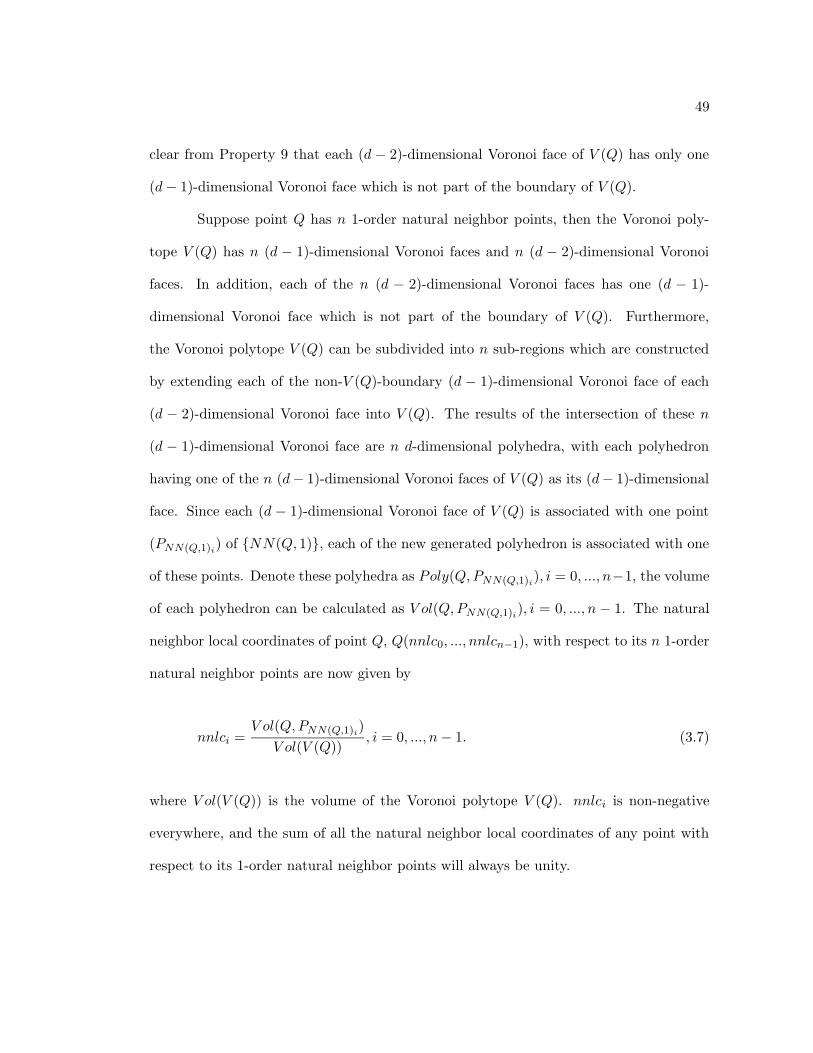
49

clear from Property 9 that each (d − 2)-dimensional Voronoi face of V (Q) has only one

(d− 1)-dimensional Voronoi face which is not part of the boundary of V (Q).

Suppose point Q has n 1-order natural neighbor points, then the Voronoi poly-

tope V (Q) has n (d − 1)-dimensional Voronoi faces and n (d − 2)-dimensional Voronoi

faces. In addition, each of the n (d − 2)-dimensional Voronoi faces has one (d − 1)-

dimensional Voronoi face which is not part of the boundary of V (Q). Furthermore,

the Voronoi polytope V (Q) can be subdivided into n sub-regions which are constructed

by extending each of the non-V (Q)-boundary (d − 1)-dimensional Voronoi face of each

(d − 2)-dimensional Voronoi face into V (Q). The results of the intersection of these n

(d − 1)-dimensional Voronoi face are n d-dimensional polyhedra, with each polyhedron

having one of the n (d− 1)-dimensional Voronoi faces of V (Q) as its (d− 1)-dimensional

face. Since each (d − 1)-dimensional Voronoi face of V (Q) is associated with one point

(PNN(Q,1)i) of NN(Q, 1), each of the new generated polyhedron is associated with one

of these points. Denote these polyhedra as Poly(Q,PNN(Q,1)i), i = 0, ..., n−1, the volume

of each polyhedron can be calculated as V ol(Q,PNN(Q,1)i), i = 0, ..., n − 1. The natural

neighbor local coordinates of point Q, Q(nnlc0, ..., nnlcn−1), with respect to its n 1-order

natural neighbor points are now given by

nnlci =V ol(Q,PNN(Q,1)i)

V ol(V (Q)), i = 0, ..., n− 1. (3.7)

where V ol(V (Q)) is the volume of the Voronoi polytope V (Q). nnlci is non-negative

everywhere, and the sum of all the natural neighbor local coordinates of any point with

respect to its 1-order natural neighbor points will always be unity.

50

A two-dimensional example of the natural neighbor local coordinates is given in

Figure 3.10. Here, point X has five 1-order natural neighbor points, A, B, E, F and

C, and Voronoi polygon V (X) has five edges and five vertices. Extending each of the

non-V (X)-edge of each vertex into V (X), we now have five sub-regions inside V (X),

with each associated with one of the five 1-order natural neighbor points. The natural

neighbor local coordinate of X with respect to A is the shaded area as a fraction of the

area of V (X).

Natural weighted smoothing/interpolation uses the natural neighbor local coordi-

nates as the weights in estimating the weighted average of the functional values at given

points from the influence points[108]. The generated function has a continuous derivative

everywhere except at the data points[135]. In the cases represented by Equation 3.2,

the weighting coefficients ωi of the corresponding influence points are the values of the

natural neighbor local coordinates of the given point. For the two-dimensional example

in Figure 3.9, we have

ωi = nnlci =V ol(Q,Fi)

V ol(V (Q)), i = 0, ..., 4. (3.8)

3.4 Modified Delaunay Tessellation

From the earlier discussion in the chapter, we know that for a given point set Pi in Rd,

the Delaunay tessellation defines a symmetrical and isotropic neighborhood relationship

between the data points, and produces a unique minimal shape representation of the point

set without a prior connectivity information. In practical application such as our LV rep-

resentation, however, the distribution of the points is often limited to a certain subspace

of Rd, and a subset of the points may have a priori connectivity relationships which need

51

Figure 3.10: Natural neighbor local coordinates. For point X, points A, B, E, F , and C

are its 1-order natural neighbor points, and the natural neighbor local coordinate of X

with respect to A is the shaded area as a fraction of area of V (X).

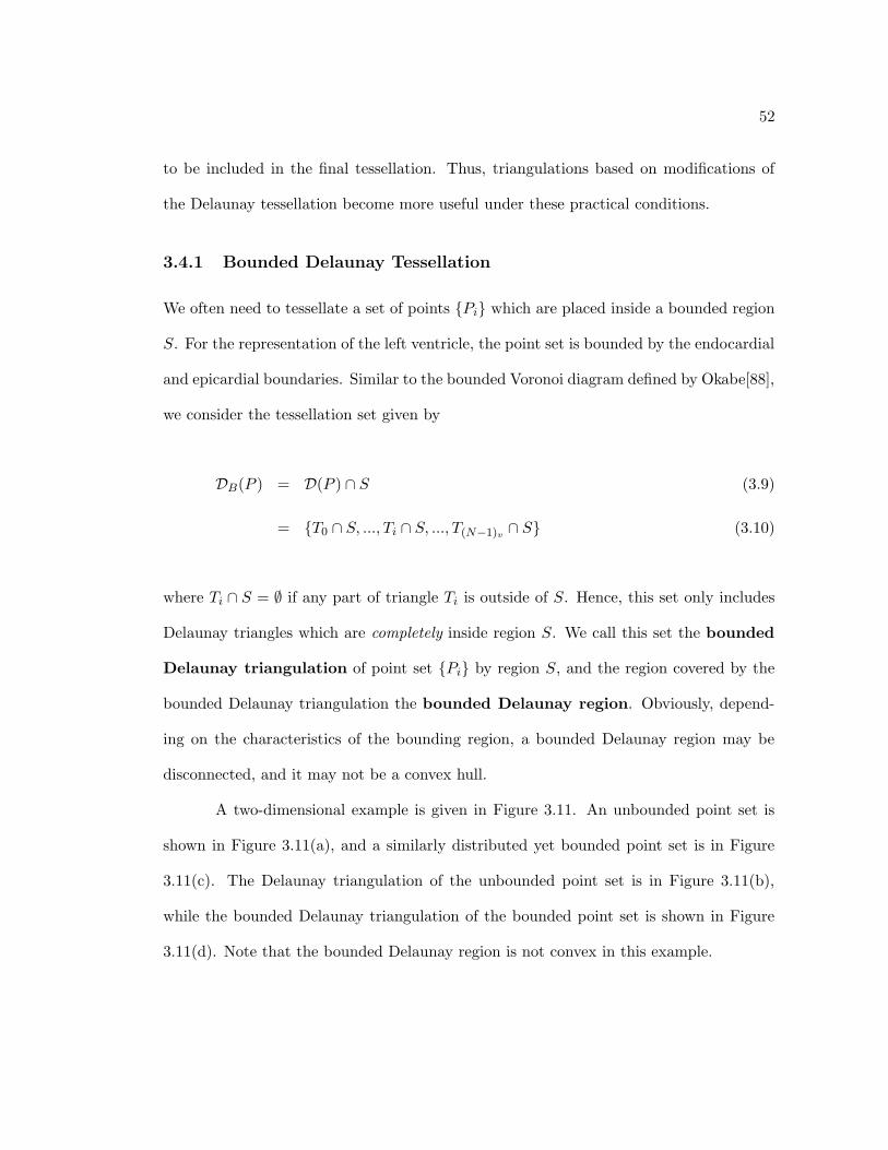
52

to be included in the final tessellation. Thus, triangulations based on modifications of

the Delaunay tessellation become more useful under these practical conditions.

3.4.1 Bounded Delaunay Tessellation

We often need to tessellate a set of points Pi which are placed inside a bounded region

S. For the representation of the left ventricle, the point set is bounded by the endocardial

and epicardial boundaries. Similar to the bounded Voronoi diagram defined by Okabe[88],

we consider the tessellation set given by

DB(P ) = D(P ) ∩ S (3.9)

= T0 ∩ S, ..., Ti ∩ S, ..., T(N−1)v ∩ S (3.10)

where Ti ∩ S = ∅ if any part of triangle Ti is outside of S. Hence, this set only includes

Delaunay triangles which are completely inside region S. We call this set the bounded

Delaunay triangulation of point set Pi by region S, and the region covered by the

bounded Delaunay triangulation the bounded Delaunay region. Obviously, depend-

ing on the characteristics of the bounding region, a bounded Delaunay region may be

disconnected, and it may not be a convex hull.

A two-dimensional example is given in Figure 3.11. An unbounded point set is

shown in Figure 3.11(a), and a similarly distributed yet bounded point set is in Figure

3.11(c). The Delaunay triangulation of the unbounded point set is in Figure 3.11(b),

while the bounded Delaunay triangulation of the bounded point set is shown in Figure

3.11(d). Note that the bounded Delaunay region is not convex in this example.

53

A

B

D

E

C

F

G

H

B

D

E

C

F

G

H

A

(a) (b)

B

D

E

C

F

G

H

AS A

B

D

E

C

F

G

H

S

(c) (d)

Figure 3.11: Bounded Delaunay triangulation. (a) and (b): an unbounded point set and

its Delaunay triangulation; (c) and (d): a bounded point set and its bounded Delaunay

triangulation. The data points are the filled dots, the bound of the region is the thick

line, and the Delaunay edges are the broken lines.

54

3.4.2 Constrained Delaunay Tessellation

There may also be cases where we deal not only with point set Pi in Rd, but also with

k-dimensional (k < d) simplicial structures Li of special topographical significance,

such as line segments and two-dimensional facets in R3, whose endpoints belong to Pi.

We want the triangulation of these points to include those k-dimensional structures as

k-dimensional faces or aggregates of several k-dimensional faces of the final triangulation.

The triangulation of Pi in this nature is called the constrained Delaunay tessella-

tion, DC(P ), of point set Pi by constraints Li, even though strictly speaking some

of triangles are no longer Delaunay triangles in the sense that the circumspheres of these

triangles are not empty[88].

If we simply compute the Delaunay triangulation of the point set, including the

endpoints of the constraint structures, these simplicial structures may not always be k-

dimensional Delaunay faces or aggregates of several k-dimensional faces of the Delaunay

structure D(P ). The modification of D(P ) which must be undertaken to create DC(P )

arises when the presence of Li in Rd affects the mutual visibility of members of Pi.

In R2, two points Pr and Ps are said to be mutually visible if the line segment

PrPs does not intersect any member of Li[88]. For example, in Figure 3.12 points P1

and P2 are mutually visible while points P2 and P4 are not. Let E be the set of edges

joining data points which are mutually visible. The DC(P ) consists of Li along with a

subset of E in which the circumball of each triangle with vertices Pr, Ps and Pt does not

contain in its interior any other point which is visible from Pr, Ps and Pt. Thus, points

P1, P2 and P3 in Figure 3.12 form a triangle of DC(P ) even though their circumcircle

contains P4 because P2 and P4 are not mutually visible. Obviously triangle P1P2P3 is

not a Delaunay triangle in strict sense. Figure 3.13 shows the two-dimensional examples

55

P1

P2

P4

P3

L1

L2

Figure 3.12: Mutual visibility criterion for defining triangles in a two-dimensional con-

strained Delaunay triangulation. L1 and L2 are line segment constraints, P1P2P3 is a

valid triangle in the DC(P ) even though their circumcircle (broken line) contains P4,

because P2 and P4 are not mutually visible

of constrained Delaunay tessellation DC(P ) along with their unconstrained counterparts

D(P ).

We extend the definition of mutual visibility into higher dimensions. For higher

dimensional cases, the definition of the mutual visibility criterion for defining valid tri-

angles is similar to the two dimensional case. Here, mutual visibility of k-dimensional

(k = 1, ..., d − 1) faces of the triangle in Rd needs to be checked against the constraint

set Li. A triangle with d + 1 vertices Pi0 , ..., Pid is a valid triangle of the constrained

Delaunay triangulation of the point set if its circumball does not contain in its interior

any other points which are visible from points Pi0 , ..., Pid .

56

(a) (b)

(c) (d)

Figure 3.13: Examples of the constrained Delaunay tessellation. (a): the unconstrained

Delaunay triangulation of the points; (b): the corresponding DC(P ) constrained by line

segments (broken lines in (a)); (c): the unconstrained Delaunay triangulation of the

points; (d): the corresponding DC(P ) constrained by a triangle (shaded area).

57

It should be pointed out that the constrained Delaunay tessellation described

above is different from the same named definition given by Faugeras[34]. In our definition,

the pre-determined constraint structures are preserved while the triangulation is not in

strict Delaunay sense. On the other hand, in [34] which only deals with 2D point set, the

constraint structures such as line segments are modified by adding as many as needed

new points to these segments in such a way that the resulting Delaunay triangulation

contains each of these line segments as a Delaunay edge (no point added to this segment)

or aggregate of Delaunay edges (points have been added to this segment). Hence, this

definition will yield true Delaunay triangulation. However, the pre-determined constraint

structures no longer exist in their original forms. We believe for our problem of LV

representation, it is more important to preserve the pre-determined structures. The first

reason is that the pre-determined structures can be often of physiological or topological

significance which are worthwhile preserving. The second reason is that the finite element

mesh need to be as uniform in size as possible, which could be difficult to achieve using

Faugeras’s definition where the points are added until the triangulation is Delaunay.

3.5 Delaunay Tessellation of Left Ventricle

As described in Section 3.2, the myocardium of the left ventricle is first defined by

the bounding endocardial and epicardial contour stacks detected from the image data.

Then, the mid-wall points are founded by using a region filling procedure of the bounded

area. Finally, these myocardial sample points, including endocardial boundary, epicardial

boundary, and mid-wall points, are tessellated to form the discrete geometrical represen-

tation of the left ventricle.

The bounded Delaunay tessellation is particularly useful in the representation

58

of the left ventricle since the myocardial volume is bounded by the endocardial and

epicardial boundaries, which are often complex geometrical shapes. The constrained

Delaunay tessellation is also useful if certain prior connectivity information is available

and needed to be preserved in the final representation.

We have concluded that if the myocardial sample point set satisfies the non-

collinearity and non-cosphericity assumptions, it is in general position and its Delaunay

tessellation is unique. However, members of the myocardial point set, especially the mid-

wall points from the region filling, are usually collinear and/or cospherical. To obtain a

unique triangulation, small Gaussian-distributed random noise is added to the x-, y- and

z-coordinates of the myocardial points to put the point set in a general position. However,

this noise-added point set is only used to determine the connectivity relationship between

the points from its Delaunay tessellation, while the coordinates of the original points still

represent the spatial locations of the sample points, and are used in the motion and

deformation algorithms described in the future chapters.

3.5.1 Two Dimensional LV Tessellation

For two-dimensional myocardial slices, the myocardium is bounded by the endocardial

and epicardial contours. Since the boundaries are in contour form, the connectivity of the

boundary points are pre-determined. The endocardial and epicardial points are connected

in an order such that the traces of the connections form the boundary contours. A bounded

and constrained Delaunay triangulation is needed for the representation of a myocardial

slice. Triangles with edges outside of the bounding region, along with triangles whose

vertices are boundary points but whose boundary-vertices-defined edges fail to comply

with the prior connectivity constraints, are rejected from the tessellation.

In the example in Figure 3.14, (a) shows the boundary contours of a myocardial

59

slice and (b) shows the whole point set along with the bounding contours. The regular

Delaunay triangulation of the point set is shown in Figure 3.14(c) with the bounding

contours in bold lines, and the bounded and constrained Delaunay triangulation is shown

in Figure 3.14(d).

3.5.2 Three Dimensional LV Tessellation

For three-dimensional myocardial point sets, the myocardium is bounded by the endo-

cardial and epicardial contour stacks, and we need to construct a volumetric tessellation.

The myocardial points at each imaging plane are bounded by the endocardial and epicar-

dial contours at that plane, and the connectivity of the boundary points at that plane are

pre-determined such that the traces of the connections form the boundary contours at

that plane. The mid-wall points are again found by using a region filling procedure within

the bounded area. However, the volumetric representation of the myocardium requires

not only in-plane connections of the sample points, but also the connections between

points which belong to different planes. Unlike the two-dimensional case, the contours at

different planes, which are unrelated to each other, cannot trivially define the bounded

region for the myocardium. We need to define the bounded myocardial region either by

explicitly forming endocardial and epicardial surfaces or implicitly by keeping/rejecting

new triangles using some inside/outside criterion, both from the contour stacks.

To explicitly form the endocardial and epicardial surfaces from the contour stacks,

a surface-from-contour-stack pre-process is needed. There are various algorithms available

to triangulate the contour stack into a polygonal representation of the surface[37, 65, 76].

Finding connections between points in successive contours is often reduced to a search

problem on a toroidal graph, and a correct surface is chosen by optimizing some objective

function. Choices of metrics for the graph cost function include maximum volume[65],

60

(a) (b)

(c) (d)

Figure 3.14: Two-dimensional Delaunay tessellation of myocardial slice. (a): the endo-

cardial and epicardial contours; (b): the myocardial sample point set; (c): the regular

Delaunay triangulation of the point set with the bounding contours in bold lines; (d): the

bounded and constrained Delaunay triangulation of the myocardium.

61

minimum area[37], minimum spanning tree[76]. These surface forming methods could

be computationally expensive if the contours are finely sampled. After the boundary

surfaces are formed, a bounded and constrained Delaunay triangulation is constructed for

the myocardial point set.

The implicit method we propose here adds additional constraints into the bounded

and constrained Delaunay triangulation process, and is in spirit close to the Delaunay

based surface-from-contour method in [16] which is only for surface triangulation.

The first criterion is that only tetrahedra which have their four vertices on two

consecutive planes, denoted as “higher-plane” and “lower-plane”, could possibly be valid.

In practice, this is achieved by Delaunay triangulation sample points two consecutive

slices at a time, then assembling them into one single aggregate. Since each tetrahe-

dron satisfies the empty circumsphere criterion, the aggregate of all the tetrahedra is a

Delaunay structure.

The second criterion determines which of the Delaunay tetrahedra are the valid

ones, judged from the endocardial and epicardial contour stacks. Tetrahedron with no

more than one vertex on the boundary contours (at least three vertices in the mid-wall)

is always considered inside the myocardium, hence is always valid. Tetrahedron with

multiple vertices on the contours is judged by the six mid-points of its edges: the mid-

points are projected upward to the higher-plane and downward to the lower-plane. If

either all upward projections are inside the bounding region of the higher-plane, or all

downward projections are inside the bounding region of the lower-plane, or both, this

tetrahedra is a valid Delaunay triangle. Otherwise, it is invalid and rejected. Since this

criterion involves only two-dimensional operation on a subset of the tetrahedron, the

computational cost of this implicit method is not very high.

62

(a) (b)

(c) (d) (e)

Figure 3.15: Three-dimensional Delaunay tessellation of myocardium. (a): the endocar-

dial and epicardial contour stacks; (b): the myocardial sample point set; (c): a two-slice

Delaunay triangulation; (d): the bounded and constrained Delaunay triangulation of

these two slices; (e): the bounded and constrained Delaunay triangulation of the my-

ocardium. (only visible Delaunay edges are shown in the figures)

In the example in Figure 3.15, (a) shows the boundary contour stacks of the

myocardium and (b) shows the whole point set. The Delaunay triangulation of points on

two consecutive slices (the first criterion) is shown in Figure 3.15(c), and the bounded and

constrained Delaunay triangulation (the second criterion) of these two slices is shown in

Figure 3.15(d). The bounded and constrained Delaunay triangulation of the entire point

set is shown in Figure 3.15(e). (only visible Delaunay edges are shown in the figures)

The by-products of the three-dimensional volumetric Delaunay triangulation of

the myocardium are the Delaunay triangulations of myocardial surfaces. The two-dimensional

63

Delaunay facets which are on the outside boundary of the triangulation constitute the

epicardial surface, while the facets which are on the inside boundary of the triangulation

constitute the epicardial surface. These surfaces are Delaunay structures because each

circumsphere contains no vertex other than the ones which belong to the facet. Examples

of triangulated myocardial surfaces are shown in Figure 3.16.

3.6 Conclusion

A geometrical representation, based on bounded and constrained Delaunay triangulation,

of the left ventricle has been developed in this chapter. This approach allows three levels

of representation of the myocardium: the sample points level, the triangulated boundary

surfaces level, and the volumetric level based upon natural neighbor relationships.

The point level representation enables the system to deal with data of differ-

ent resolutions, e.g. Dynamic Spatial Reconstructor images, magnetic resonance images,

echocardiographic images. The surfaces level representation makes it possible to analyze

boundary shape characterization and motion. The volumetric level representation facili-

tates the incorporation of continuum mechanical models and other physical constraints,

as well as the adoption of a finite element framework as the unified approach to integrate

complementary information. The multi-order natural neighbor relationship between the

sample points also provides natural multi-order interpolation, smoothing, and function

fitting schemes weighted by natural neighbor coordinates, to further study the character-

istics of a set of spatial points.

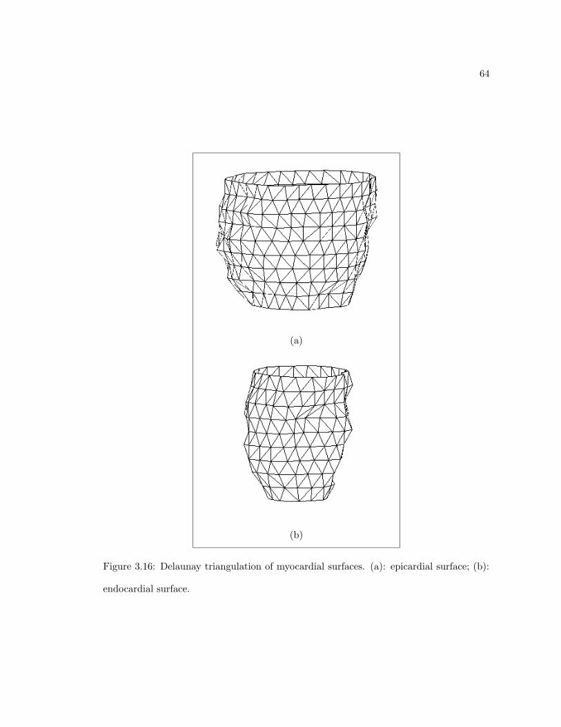
64

(a)

(b)

Figure 3.16: Delaunay triangulation of myocardial surfaces. (a): epicardial surface; (b):

endocardial surface.

Chapter 4

Boundary Motion Analysis

4.1 Introduction

In this chapter, we will build a system which establishes dense field point correspondences

between successive myocardial surfaces over the entire cardiac cycle. Further analysis of

the motion parameters of normal and infarcted hearts also inspire new ways to predict

the location and extent of myocardial injury from in vivo measurement.

Without prior motion knowledge, one can hypothesize that point matching and

tracking between successive surfaces should follow a minimum energy principle, which

means that a point should move and deform as little as possible. Since the myocardial

surface undergoes global motion as well as local motion and deformation, purely mini-

mum distance based approaches[95, 54] often fail to produce consistently good matches,

especially for the endocardial surface where motion and deformation are often relatively

larger. However, if the temporal sampling is fine enough, sixteen frames per cardiac

cycle for our data, it has been tested and validated that shape landmarks are good track-

ing cues over time[120]. The hypothesis is that for short time intervals, the differential

65

66

shape characteristics at surface points, especially the geometrically significant points such

as highly curved ones, should not change dramatically between successive frames. The

shape features may be more reliable matching cues than the distance measures. How-

ever, pure local matching methods often produce incoherent, even conflicting, motion

vectors between neighboring surface points. To alleviate this problem, local smoothness

constraints, which assume that neighboring surface points should have similar motion

characteristics and vary only gradually, are often built into the matching process.

We propose a shape-based motion tracking approach to track the motion tra-

jectories of a dense field of points over the entire cardiac cycle, based on locating and

matching differential geometric features and an ideal-thin-plate bending model of local

surface patches. The surface characterization is performed by multi-scale fittings of multi-

order natural neighbor points. The local smoothness constraint is enforced to achieve a

smooth dense motion field.

For validation purposes, canine experiments have been performed using two dif-

ferent imaging modalities. Point tracking accuracy is validated using the gold-standard

motion of implanted imaging-opaque markers. The differences of two motion-derived pa-

rameters, path length and wall thickening measures, between baseline and post-infarct

data are quantified to assess regional myocardial viability, and are validated using gold-

standard post mortem TTC staining of cardiac perfusion activity.

4.2 Triangulated Surface Smoothing

As described in the previous chapter, the myocardial boundary surfaces can be represented

by the aggregate of all the two-dimensional Delaunay facets which are on the boundary

of the volumetric Delaunay triangulation of the myocardium. These polyhedral surfaces,

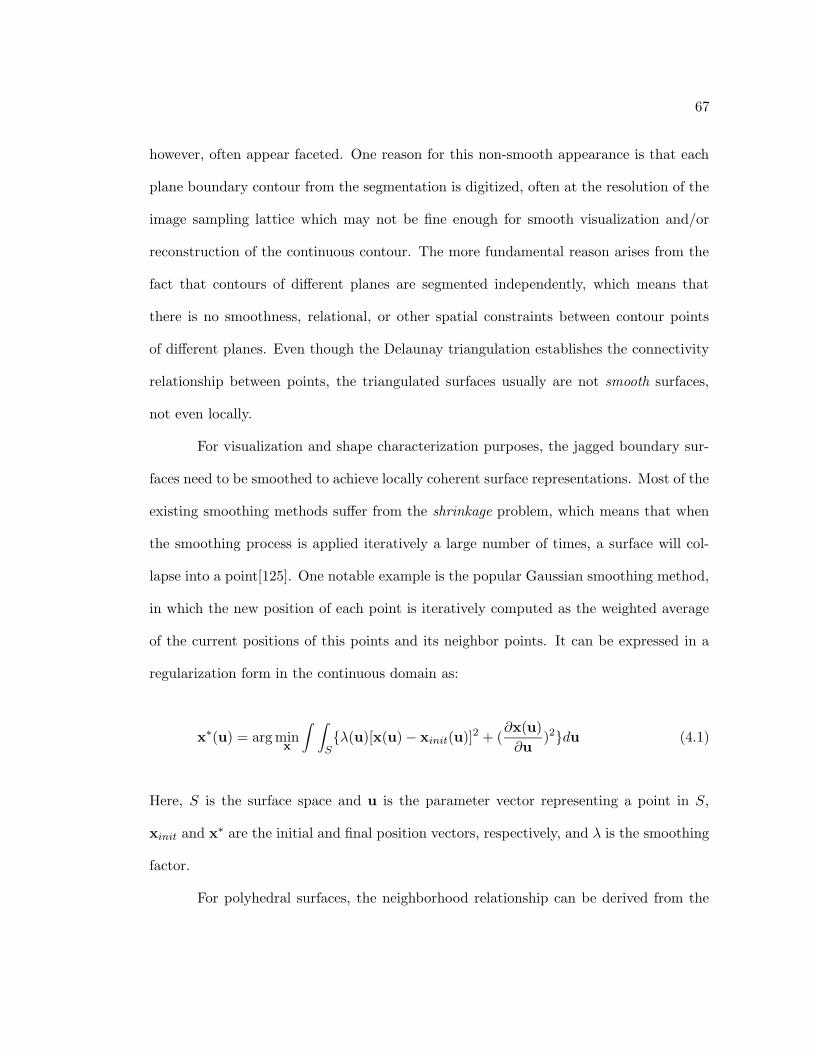
67

however, often appear faceted. One reason for this non-smooth appearance is that each

plane boundary contour from the segmentation is digitized, often at the resolution of the

image sampling lattice which may not be fine enough for smooth visualization and/or

reconstruction of the continuous contour. The more fundamental reason arises from the

fact that contours of different planes are segmented independently, which means that

there is no smoothness, relational, or other spatial constraints between contour points

of different planes. Even though the Delaunay triangulation establishes the connectivity

relationship between points, the triangulated surfaces usually are not smooth surfaces,

not even locally.

For visualization and shape characterization purposes, the jagged boundary sur-

faces need to be smoothed to achieve locally coherent surface representations. Most of the

existing smoothing methods suffer from the shrinkage problem, which means that when

the smoothing process is applied iteratively a large number of times, a surface will col-

lapse into a point[125]. One notable example is the popular Gaussian smoothing method,

in which the new position of each point is iteratively computed as the weighted average

of the current positions of this points and its neighbor points. It can be expressed in a

regularization form in the continuous domain as:

x∗(u) = argminx

∫ ∫

Sλ(u)[x(u)− xinit(u)]

2 + (∂x(u)

∂u)2du (4.1)

Here, S is the surface space and u is the parameter vector representing a point in S,

xinit and x∗ are the initial and final position vectors, respectively, and λ is the smoothing

factor.

For polyhedral surfaces, the neighborhood relationship can be derived from the

68

connectivity between the points. Hence, we approximate the derivative by the weighted

average finite differences performed on the neighboring points:

∂x(u)

∂u=

N−1∑

i=0

ωix(u)− x(ui), i = 0, ..., N − 1 (4.2)

N−1∑

i=0

ωi = 1 (4.3)

where ui is the neighbor point set, and ωi is the weighting coefficient set associated

with the neighbor points. Furthermore, the discrete version of Equation 4.1 can be

conveniently posed as a series of linear equations with the local surface patch defined by

the triangulation. The linear equations can be solved iteratively for each point x(u) by:

xnew = (1− λ′)xcurrent + λ′N−1∑

i=0

ωixi (4.4)

λ′ =1

λ+ 1(4.5)

Since the method is very local, Gaussian smoothing often has to be applied itera-

tively a large number of times in order to obtain the desired smoothing effect. However,

this also produces significant shrinkage as a by-product. A two-stage Gaussian smoothing

algorithm has been proposed by Taubin[125] to reduce the shrinkage effect, and can be

expressed as:

xnew1 = (1− λ′1)xcurrent + λ′1

N−1∑

i=0

ωixi (4.6)

xnew2 = (1− λ′2)xnew1 + λ′2

N−1∑

i=0

ωixi (4.7)

69

For each iterative smoothing step, after a first Gaussian smoothing stage with a posi-

tive smoothing factor λ′1 which produces a slightly shrunk surface, a second Gaussian

smoothing stage is applied with a negative smoothing factor λ′2 which produces a slightly

expanded surface. λ′2 has slightly greater magnitude than λ′1 (0 < λ′1 < −λ′2), with the

difference determined by a bounded band which makes sure that the surface does not

shrink or expand after each two-stage smoothing. This new method is in fact a linear

low-pass filter that removes high curvature variations, with the two smoothing factors

determining the passing band.

Figure 4.1 shows the different effects of traditional Gaussian smoothing and two-

stage non-shrinkage smoothing. The original triangulated endocardial surface is shown

in Figure 4.1(a) (rendered) and Figure 4.1(b) (wireframe). The next three figures on the

right side are the smoothing results for the traditional Gaussian smoothing process (λ′ =

0.33, iteration number n = 10 (Figure 4.1(d)), 50 (Figure 4.1(f)), and 100 (Figure 4.1(h)).

The three figures on the left side are the smoothing results for the two-stage non-shrinkage

Gaussian smoothing process (λ′1 = 0.33, λ′2 = −0.34, iteration number n = 10 (Figure

4.1(c)), 50 (Figure 4.1(e)), and 100 (Figure 4.1(g)). In both smoothing procedures, the

z-coordinates of the points in top and bottom contours are fixed. It is quite obvious, at

least visually, that the non-shrinkage process keeps the overall size and shape-feature of

the surface while the traditional Gaussian smoothing produces severe shrinkage when the

iteration number becomes large. Because the relative positions of neighbor points are

better preserved in the non-shrinkage process, the geometrical structure of the surface is

also better preserved.

The weighting coefficients of the neighbor points are often set to be the normal-

ized values (the sum of the weighting coefficients equals to unity) which are inversely

70

(a) (b)

(c) (d)

(e) (f)

(g) (h)

Figure 4.1: Regular and non-shrinkage Gaussian smoothing of triangulated surface. (a):

the original triangulated endocardial surface (rendered); (b): the wireframe of the original

surface; (c)(e)(g): non-shrinkage Gaussian smoothing results with λ′1 = 0.33, λ′2 = −0.34

and iteration number n = 10 (c), 50 (e), and 100 (g); (d)(f)(h): regular Gaussian smooth-

ing results with λ′ = 0.33, and iteration number n = 10 (d), 50 (f), and 100 (h).

71

proportional to the distances between the fiducial point and its neighbor points[125]. It

has been shown experimentally that the weighting coefficients determined this way are

usually good enough for visualization purposes, even though it may be troublesome for

non-uniformly distributed point sets where distances no longer reflects the true geomet-

rical influence between points. However, if the purpose is to recover the true geometry of

the noisy surface, we need to choose weighting coefficients which are more closely related

to the geometry of the local point distributions. The natural neighbor coordinates dis-

cussed in chapter 3, which quantitatively express the geometrical position of any point

relative to each of its natural neighbor points, become good candidates:

ωi = nnlci (4.8)

An experiment using a synthetic ellipsoidal surface is conducted to demonstrate

the advantage of using natural neighbor coordinates as the weighting coefficients. Two

ellipsoidal surfaces with axis lengths 10, 10, and 20 are synthetically generated. One

surface is spatially uniformly sampled (Figure 4.2(a)), and the other one is non-uniformly

sampled (Figure 4.3(a)). Each of the sample points is then rounded off to its nearest lattice

point to mimic the quantization effect (Figure 4.2(c) and Figure 4.3(c)), with the average

distance error being 0.826 ± 0.500 for the uniformly sampled surface and 0.769 ± 0.465

for the non-uniform one. The distance weighted smoothing and the natural weighted

smoothing are applied to the two surfaces over several different number of iterations, and

the results are shown in Table 4.1. These results clearly show that the natural weighted

smoothing is far superior in the recovery of the true geometry, the ellipsoidal surfaces in

this experiment, from noisy surface approximations with both uniform and non-uniform

72

Error After Smoothing

Surface Quantization Iteration Distance Natural

Type Error Number Weighted Weighted

Uniformly 10 0.814±0.469 0.340±0.116

Sampled 0.826±0.500 50 0.774±0.456 0.272±0.103

100 0.731±0.443 0.215±0.095

Non-uniformly 10 0.791±0.440 0.332±0.093

Sampled 0.769±0.465 50 0.682±0.419 0.274±0.085

100 0.641±0.387 0.222±0.067

Table 4.1: Comparison of distance and natural weighted smoothing. The error

(mean±standard deviation) is the distance between sample points and their true po-

sitions before roundoff.

sampling.

The visual results of this experiment are shown in Figure 4.2 for the uniformly

sampled surface, and in Figure 4.3 for the non-uniformly sampled surface. The left col-

umn figures are the rendered surfaces, and the right column ones are the corresponding

wireframes. The top figures are the ideal surfaces, the second row figures are the quan-

tized noisy surfaces, the third rows are the smoothed surfaces using distance weighted

coefficients, and the bottom figures are the results from the natural weighted smoothing.

Visually, it seems that two smoothed surfaces are quite similar in the uniformly sampled

73

(a) (b)

(c) (d)

(e) (f)

(g) (h)

Figure 4.2: Distance and natural weighted smoothing of uniformly sampled ellipsoidal

surface. On the right are the rendered surfaces, and the corresponding wireframes are on

the left. (a)(b): ideal surface; (c)(d): quantized noisy surface; (e)(f): smoothed surface

using distance weighted coefficients; (g)(h): smoothed surface using natural weighted

coefficients. (smoothing factors: λ′1 = 0.33, λ′2 = −0.34; iteration number: n = 10)

74

(a) (b)

(c) (d)

(e) (f)

(g) (h)

Figure 4.3: Distance and natural weighted smoothing of non-uniformly sampled ellipsoidal

surface. On the left are the rendered surfaces, and the corresponding wireframes are on

the right. (a)(b): ideal surface; (c)(d): quantized noisy surface; (e)(f): smoothed surface

using distance weighted coefficients; (g)(h): smoothed surface using natural weighted

coefficients. (smoothing factors: λ′1 = 0.33, λ′2 = −0.34; iteration number: n = 10)

75

(a) (b)

(c) (d)

(e) (f)

(g) (h)

Figure 4.4: Natural weighted non-shrinkage smoothing of myocardial surfaces. On the

left are the rendered surfaces, and the corresponding wireframes are on the right. (a)(b):

original endocardial surface; (c)(d): smoothed endocardial surface; (e)(f): original epi-

cardial surface; (g)(h): smoothed epicardial surface. (smoothing factors: λ′1 = 0.33,

λ′2 = −0.34; iteration number: n = 50)

76

case, while the natural weighted smoothed surface looks smoother in the non-uniform

case.

Finally, examples of the natural weighted smoothed endocardial and epicardial

surfaces are shown in Figure 4.4.

4.3 Shape Characterization

In this section, we will discuss the characterization of local surface properties which will

be used in the surface matching process.

4.3.1 Differential Geometry of Surface

Classical differential geometry studies the local properties of curves and surfaces. These

local properties depend only on the behavior of the curve or surface in the neighborhood

of the fiducial point, and can be derived using differential calculus. The following is a

brief review of the relevant topics in differential geometry. Formal discussion can be found

in do Carmo[29] and Besl[13].

A general regular surface S ⊂ R3 is defined as: for each p ∈ S, there exists a

neighborhood V in R3 and a map x : U → V⋂

S of an open set U ⊂ R2 onto V⋂

S ⊂ R3

such that

• x(u, v) = (x(u, v), y(u, v), z(u, v)), (u, v) ∈ S is differentiable. (This condition en-

sures that a differential process can be performed on S.)

• x is a homeomorphism. And since x is continuous by the previous condition, this

means that x has an inverse x−1 : V⋂

S → U which is continuous; that is, x−1

is the restriction of a continuous map F : W ⊂ R3 → R2 defined on an open

set W containing V⋂

S. (This condition prevents self-intersections in S, and also

77

means that objects defined in terms of a parameterization do not depend on this

parameterization but rather only on the set S itself.)

• For each q ∈ U , the differential dxq : R2 → R3 is one-to-one. (This condition

guarantees the existence of a tangent plane at all points of S).

The mapping x is called a parameterization or a system of local coordinates in a neighbor-

hood of p. The neighborhood V⋂

S of p in S is called a coordinate neighborhood. From

this definition, each point p of a regular surface belongs to a coordinate neighborhood.

The points of such a neighborhood are characterized by their coordinates, therefore, we

are able to define the local properties in terms of these coordinates.

The plane dxq, which passes through x(q) = p, does not depend on the parame-

terization x. This plane is called the tangent plane to S at p, and is denoted by Tp(S).

The choice of the parameterization x determines a basis (∂x/∂u)(q), (∂x/∂v)(q), or

xu(q),xv(q), of Tp(S), called the basis associated to x. Similarly, a unit normal vector

at point x(q) = p of S is determined by

Np =xu ∧ xv|xu ∧ xv|

(q) (4.9)

where ∧ denotes cross product.

First Fundamental Form[29]: the quadratic form

Ip(w) = < w,w >p = |w|2 ≥ 0 (4.10)

is called the first fundamental form of the regular surface S ⊂ R3 at p ∈ S, where

w ∈ Tp(S), and <,> denotes inner product.

78

In the basis xu,xv associated with a parameterization x(u, v) at p, the tangent

vector w ∈ Tp(S) is the tangent vector to a parameterized curve α(t) = x(u(t), v(t)), t ∈

(−ε, ε), with p = α(0) = x(u0, v0), we obtain

Ip(α′(0)) = < α′(0), α′(0) >p (4.11)

= < xuu′ + xvv

′,xuu′ + xvv

′ >p (4.12)

= Eu′2+ 2Fu′v′ +Gv′

2(4.13)

where the values of the functions involved are computed for t = 0, and

E(u0, v0) = < xu,xu >p (4.14)

F (u0, v0) = < xu,xv >p (4.15)

G(u0, v0) = < xv,xv >p (4.16)

are the coefficients of the first fundamental form in the basis xu,xv of Tp(S). By

letting p run in the coordinate neighborhood corresponding to x(u, v), we obtain functions

E(u, v), F (u, v), G(u, v) which are differentiable in that neighborhood.

The first fundamental form is the expression of how the surface S inherits the

natural inner product of R3. It measures the small amount of movement on the surface

for a given small movement in the parameter space. Geometrically, it allows us to make

measurements on the surface without referring back to the ambient surface R3 where the

surface lies. It is invariant to surface parameterization and to translation and rotation of

the surface. Therefore, it determines the intrinsic properties of the surface.

79

Second Fundamental Form[29]: the quadratic form defined in Tp(S) by

IIp(w) = − < dNp(w), w > (4.17)

is called the second fundamental form of the regular surface S ⊂ R3 at p ∈ S, where

w ∈ Tp(S).

Again, in the basis xu,xv associated with a parameterization x(u, v) at p,

the tangent vector w ∈ Tp(S) is the tangent vector to a parameterized curve α(t) =

x(u(t), v(t)), t ∈ (−ε, ε), with p = α(0) = x(u0, v0). To simplify the notation, we invoke

the convention that all functions below denote their values at the point p.

The tangent vector to α(t) at p is

α′ = xuu′ + xvv

′ (4.18)

and

dNp(α′) = N ′(u(t), v(t)) = Nuu

′ +Nvv′ (4.19)

Therefore, the second fundamental form in the basis xu,xv is given by

IIp(α′) = − < dNp(α

′), α′ > (4.20)

= − < Nuu′ +Nvv

′,xuu′ + xvv

′ > (4.21)

= eu′2+ 2fu′v′ + gv′

2(4.22)

80

where

e = − < Nu,xu >=< N,xuu > (4.23)

f = − < Nv,xu >=< N,xuv >= − < Nu,xv > (4.24)

g = − < Nv,xv >=< N,xvv > (4.25)

are the coefficients of the second fundamental form in the basis xu,xv of Tp(S).

The second fundamental form measures the correlation between the change in

the normal vector and the change in the surface position, as a function of a given small

movement in the parameter space. Unlike the first fundamental form, it is dependent

on the embedding of the surface in space, and determines the extrinsic properties of the

surface.

Weingarten Mapping[29]: the matrix in the form

[β] = −

e f

f g

E F

F G

−1

(4.26)

is called the Weingarten mapping matrix or the shape operator matrix of the surface. This

matrix combines the first and second fundamental forms into one matrix, and determines

surface shape by relating the intrinsic geometry of the surface to the Euclidean (extrinsic)

geometry of the embedding space.

The Gaussian curvature of a surface can be defined from the Weingarten mapping

81

matrix as its determinant:

K = det[β] =eg − f2

EG− F 2(4.27)

Meanwhile, the mean curvature of a surface is similarly defined as half of the trace of the

Weingarten mapping matrix:

H =tr[β]

2=eG− 2fF + gE

2(EG− F 2)(4.28)

Since the surface curvatures are the only natural algebraic invariants of the Weingarten

mapping matrix, they arise naturally in a detailed analysis of surface shape. Gaussian and

mean curvatures are invariant to arbitrary choice of parameterization of a surface, and

are also invariant to arbitrary rotations and translations of the surface in space. These

invariances are extremely important in uniquely characterizing the view-independent sur-

face shape properties. The analysis of the left ventricular surfaces is based upon these

invariances for characterizing their shape properties.

Another way to study surface curvatures is based on the space curves that lie on

the surface. At each point p ∈ S, there is a direction of maximum normal curvature and

a direction of minimum normal curvature for all curves which

• lie on the surface;

• pass through point p;

• have normals that align with the surface normal Np at the point p.

We denote (κ1, e1) the maximum principal curvature and its direction (the magnitude and

direction of the maximum of the normal curvature function), and (κ2, e2) the minimum

82

principal curvature and its direction (the magnitude and direction of the minimum of

the normal curvature function). The principal curvatures are the two eigenvalues of the

Weingarten mapping matrix, with their directions the two eigenvectors. They are also

related to the Gaussian and mean curvatures in describing the magnitude of the surface

shape since:

K = κ1κ2 (4.29)

H =κ1 + κ2

2(4.30)

κ1 = H +√

H2 −K (4.31)

κ2 = H −√

H2 −K (4.32)

Moreover, the principal curvatures also provide the directional information of the surface

shape, which could be important in finding certain higher order differential features of

the surface, such as ridge lines.

The signs of the Gaussian, mean and principal curvatures are often used to deter-

mine basic surface types and singular points such as umbilical points[13]. Furthermore,

the numerical relationship between the two principal curvatures are used in more detailed

classification of surfaces by Koenderink[67]. A shape index function is defined as

si =2

πarctan

κ2 + κ1κ2 − κ1

, (κ2 ≥ κ1) (4.33)

All surface patches, except for plane patches where the two principal curvatures equal

zero, are mapped onto si ∈ [−1,+1]. This shape index function has many nice properties

with regards to the classification of surface types:

83

Surface Type Shape Index Range

Spherical Cup si ∈ [−1,−7/8)

Trough si ∈ [−7/8,−5/8)

Rut si ∈ [−5/8,−3/8)

Saddle Rut si ∈ [−3/8,−1/8)

Saddle si ∈ [−1/8,+1/8)

Saddle Ridge si ∈ [+1/8,+3/8)

Ridge si ∈ [+3/8,+5/8)

Dome si ∈ [+5/8,+7/8)

Spherical Cap si ∈ [+7/8,+1]

Table 4.2: Discrete surface classification using shape index function.

• The shape index is scale invariant, i.e. two spherical patches with different radii

will have same shape index values.

• Convexities and concavities are on the opposite sides of the shape index scale,

separated by saddle-like shapes.

• Two shapes from which the shape index differs only in sign represent complementary

pairs will fit to each other as stamp and mold if they are of same scale.

One discrete surface classification scheme using the shape index function is proposed in

[67]. Here, surfaces are classified into nine types as in Table 4.2.

84

spherical trough rut saddle saddle saddle ridge dome spherical cup rut ridge cap

Figure 4.5: A color spectrum represents the discrete surface types.

A color spectrum representing these nine discrete surface types is shown in Figure

4.5. We will use this color scale to visualize the shape-classified myocardial surfaces in

later sections.

4.3.2 Shape Characterization of Triangulated Surfaces

4.3.2.1 Local Surface in Graph Form

For a regular surface S ⊂ R3 and p ∈ S, there always exists a neighborhood V of p in S

such that V is the graph of a differentiable function which has one of the following three

forms[29]:

z = h(x, y) (4.34)

y = s(x, z) (4.35)

x = t(y, z) (4.36)

85

Hence, given a point p of a surface S, we can choose the coordinate axis of R3 such

that the origin O of the coordinates is at p and the z axis is directed along the outward

normal of S at p (thus, the xy plane agrees with the tangent plane Tp(S)). It follows that

a neighborhood of p in S can be represented in the form z = h(x, y), (x, y) ∈ U ⊂ R2,

where U is an open set and h is a differentiable function, with h(0, 0) = 0, hx(0, 0) =

0, hy(0, 0) = 0.

In this case, the local surface is parameterized by

x(u, v) = (u, v, h(u, v)), (u, v) ∈ U (4.37)

where u = x, v = y. It can be shown that

xu = (1, 0, hu) (4.38)

xv = (0, 1, hv) (4.39)

xuu = (0, 0, huu) (4.40)

xuv = (0, 0, huv) (4.41)

xvv = (0, 0, hvv) (4.42)

Thus, the normal vector at (x, y) is

N(x, y) =(−hx,−hy, 1)

(1 + h2x + h2y)1/2

(4.43)

From the above expressions, it is easy to obtain the coefficients of the first and second

86

fundamental forms as

E(x, y) = 1 + h2x (4.44)

F (x, y) = hxhy (4.45)

G(x, y) = 1 + h2y (4.46)

e(x, y) =hxx

(1 + h2x + h2y)1/2

(4.47)

f(x, y) =hxy

(1 + h2x + h2y)1/2

(4.48)

g(x, y) =hyy

(1 + h2x + h2y)1/2

(4.49)

Hence, the curvatures of the surface can be derived from the Weingarten mapping matrix

computed from these coefficients.

4.3.2.2 Multi-Order Local Surface Fitting

For the triangulated discrete surfaces that we are dealing with, regular continuous surfaces

are approximated by Delaunay surface triangulations of sets of points in R3. To be able to

analyze the local shape properties of point p in a neighborhood of a triangulated surface,

polynomials are usually used to approximate this neighborhood, often in the form of the

graph of a differentiable function.

We begin the process by defining a local surface patch at point p as a discrete

surface triangulation consisting of the point itself, the fiducial point, and a set of neigh-

boring 3D points of p. Two questions arise for constructing a smooth local surface for

these points:

1. How do we define the neighborhood of the fiducial point?

87

2. How do we define the parameterization of the surface patch?

The second question has an easier answer, that is we want this local surface to be

represented by the graph of a differentiable function. For this reason, we choose a local

coordinate system with its origin at the fiducial point p, and the z axis in the normal

direction of the surface S in p. The estimated normal at p is determined as the weighted

average of the normals of all the Delaunay facets which have p as one of their Delaunay

vertices. The weighting coefficient for each facet is its normalized area. To make the

normal directions consistent among all the points on the entire surface, we would like

to have the outward normals. Since the xy plane agrees with the tangent plane Tp(S),

we may choose any pair of orthogonal directions as the x and y axes. After this local

reference coordinate system is established, the local surface can be represented in the

graph form z = h(x, y), which is a one-to-one R2 → R mapping if the neighborhood of p

is well chosen.

Traditionally, the neighborhood of point p is defined as a sphere centered at p with

a radius R in R3, and all the points that fall inside this sphere constitute the local surface

point set[4, 109]. However, depending on the value of R and the roughness and folding of

the local surface, z = h(x, y) may not be a unique function. Figure 4.6 shows the possible

multiple mapping problem in a 2D representation. In this example, the surface patch

defined from the neighborhood folds around p, and causes the graph function to have

multiple mappings in R2 for one value in R. And since this nearest Euclidean distance

based method does not take account of the known connectivity from triangulation, it may

also include points which are disconnected from the valid surface points and should not

be in the neighborhood of p at all (they are parts of other local surface patches), such as

the case shown in Figure 4.7. Of course, these two problems can be avoided by choosing

88

z = h(x,y)

xy Plane

R

p

Multiplemappings

Figure 4.6: Possible multiple mappings in the graph representation of surface patch.

The surface is the solid line, with the surface points the filled dots (they are inside the

neighborhood sphere). The local reference frame has p as origin, the normal direction at

p as z axis, and the tangent plane as xy plane. Obviously, the graph function z = h(x, y)

is not a unique mapping.

small radius R. However, the determination of the value for R is a difficult task without

the knowledge about the geometry of the underlying surface, which is exactly what we

are trying to estimate.

In order to choose a neighborhood of p which is unique (no folding) and local

(no non-neighboring points), the natural neighbor relationship between surface points

is needed to define a more precise and flexible neighborhood. First of all, if we choose

only the 1-order natural neighbors as the neighborhood of p, the graph function will

almost always have a unique mapping (only when the point distribution is extremely

89

z = h(x,y)

xy Plane

R

p

Invalidpoints

Figure 4.7: Invalid neighborhood points. The valid surface points are the filled dots, while

the unfilled dots are invalid points even though they are inside the neighborhood sphere.

From the connectivity provided by triangulation, the unfilled dots are disconnected from

the valid surface points, and belong to another surface patch.

ill-conditioned will the Delaunay facets fold to each other with respect to the normal

direction). If the local surface is well-behaved, which means that the orientation of

one facet does not change dramatically from those of its adjacent facets, higher orders of

natural neighbor points can also be included in the neighborhood of p. Depending on how

many orders of natural neighbor points are included in the neighborhood, the local surface

can be considered to have multi-scale details. Secondly, the natural connectivity ensures

that only valid neighbor points will be chosen, since each of these points is connected to

at least one other chosen point. This is true even if higher order natural neighbor points

are included in the neighborhood.

90

Since the Weingarten mapping matrix only depends on the first and second deriva-

tives of the graph function h(x, y), biquadratic functions are all we need to estimate the

curvatures of the local surface, assuming that the local surfaces are well behaved such

that a biquadratic polynomial can approximate a patch sufficiently closely. The neigh-

borhood points are embedded in the local coordinate system, which has p as the origin,

the outward normal as the z axis, and two tangent directions as x and y axes. The

estimate of the biquadratic graph function involves finding the five coefficients of the

polynomial[4, 109]:

z = h(x, y) = a1x2 + a2xy + a3y

2 + a4x+ a5y (4.50)

If there are at least four neighboring points, say n − 1 (n ≥ 5) points, the least-square

estimate of the five coefficients is evident. In matrix form, the coefficient vector ~a which

minimizes the fit error is:

~a = (ATA)−1AT ~Z (4.51)

where A is a n x 5 matrix with row i being [x2i xiyi y2i xi yi], ~Z is a column vector of

the zi values. Once the coefficient vectors are found, computing the actual differential

properties on the fiducial point is straightforward.

The graph function estimation and curvature estimation may also follow a multi-

scale procedure, depending on how many orders of natural neighbor points are included

in the neighborhood. We denote the k-scale graph function as the one estimated from

the neighborhood which includes 0-order, ..., k-order natural neighbor points. If certain

prior information is available, we could use a lower scale (small k) graph function to

91

characterize highly curved surfaces to avoid the smoothing effect, and use a higher scale

(large k) graph function to characterize flat surfaces to alleviate the noise effect. The

consistency of the estimated shape characteristics through different scales, such as from

higher to lower, may also indicate the goodness and reliability of predominant shape

features (corners, ridge lines, etc) in the surface.

Figure 4.8 shows the Gaussian curvature, mean curvature, the two principal cur-

vatures, and the shape index maps of an endocardial surface derived from 1-scale, 2-scale

and 3-scale graph functions. Similar maps of an epicardial surface are shown in Figure

4.9. It is clear that the shape patterns are generally consistent across different scales.

The curvature maps from lower scale graph functions (small neighborhood) appear nois-

ier than curvature maps from higher scale graph functions (large neighborhood), while

the latter ones may over-smooth the surface shape features.

4.4 Surface Motion Field

The movement over the cardiac cycle of a set of LV surface points is determined by

following local surface shape between successive surface frames. In the first step of the

tracking algorithm, endocardial and epicardial surfaces at one given time instant are used

as reference surfaces and are subsampled, creating a sparser set of points (the later shown

experimental results are obtained using ten percent sampling rate). The reason to use

this sparse set of points for initial match is to avoid cross-overs between local matches. If

the search windows are well chosen (discussed later in the section), the sparse point set

usually does not create the cross-over problem. Efforts have been made to choose more

points from highly curved regions and fewer points from flat regions by thresholding the

curvature values. Under the assumption that the LV surface deforms as little as possible

92

(a) (b) (c)

Figure 4.8: Shape maps of an endocardial surface derived from multi-scale graph func-

tions. Column (a) is for the 1-scale, column (b) is for the 2-scale, and column (c) is for the

3-scale graph functions. From top to bottom row: Gaussian curvature, mean curvature,

maximum principal curvature, minimum principal curvature, and shape index maps. For

the curvature maps, the values from negative to positive are represented by a continuous

color spectrum from red to green. The value-to-color scale is the same for all three maps

within each row, but it is different between different curvatures. The shape index maps

use the color scale shown in Figure 4.5.

93

(a) (b) (c)

Figure 4.9: Shape maps of an epicardial surface derived from multi-scale graph functions.

Column (a) is for the 1-scale, column (b) is for the 2-scale, and column (c) is for the

3-scale graph functions. From top to bottom row: Gaussian curvature, mean curvature,

maximum principal curvature, minimum principal curvature, and shape index maps. For

the curvature maps, the values from negative to positive are represented by a continuous

color spectrum from red to green. The value-to-color scale is the same for all three maps

within each row, but it is different between different curvatures. The shape index maps

use the color scale shown in Figure 4.5.

94

between small time intervals, the subsampled surface points are matched and followed

over the LV surface sequences under a minimum bending energy model. These initially

calculated 3D displacement vectors can be noisy due to inherent data noise and matching

uncertainty. Match-confidence-weighted regularization functionals are utilized to help

limit these problems and to compute the dense field motion for all the surface points.

4.4.1 Thin Plate Bending Model

Local surface patches on the LV are modeled as thin flexible plates, loosely constrained to

deform in a predetermined fashion which will be defined in the next section. The potential

energy of an ideal thin flexible plate of elastic material is a measure of the strain energy

of the deformation from its equilibrium state, a plane. It is a function of the two principal

curvatures of the plate, and is invariant to 3D rotation and translation[25]:

ε = Aκ21 + κ22

2(4.52)

where A is a material related constant, and κ1 and κ2 are the two principal curvatures

of the surface patch of interest. Note that even though the principal curvatures have

associated directions, only their magnitudes are relevant in the potential energy metric.

Also, the potential energy function does not differentiate the different types of surfaces

classified by the shape index function.

Figure 4.10 shows the potential energy maps and the shape index maps of two

ellipsoidal surfaces estimated from the shape characterization procedure discussed in Sec-

tion 4.3, one with axis lengths 10, 10, 20, and the other one with 5, 5, 10. Even though

the potential energy is not invariant to scale (the smaller ellipsoid has larger potential

energy), their shape index maps are virtually the same. The potential energy maps of an

95

(a) (b)

(c) (d)

Figure 4.10: Potential energy and shape index maps of ellipsoidal surfaces. (a) and (b):

potential energy map (a) and shape index map (b) of an ellipsoidal surface with axis

lengths 10, 10, 20; (c) and (d): potential energy map (c) and shape index map (d) of an

ellipsoidal surface with axis lengths 5, 5, 10. The potential energy maps have the same

color scale: green for larger values, white for smaller values.

endocardial surface over the entire cardiac cycle (sixteen temporal sampling frames) are

shown in Figure 4.11, and the maps of an epicardial surface are shown in Figure 4.12.

In these maps, most of the high potential energy features run through several temporal

frames or even the entire sequence. This consistency of shape feature (the potential en-

ergy) over time provides the basis for visually matching surface points based upon shape

cues (in this case, the potential energy).

96

(a) (b) (c) (d)

(e) (f) (g) (h)

(i) (j) (k) (l)

(m) (n) (o) (p)

Figure 4.11: Potential energy maps of an endocardial surface over the entire cardiac cycle.

The temporal sequence of the maps runs from top to bottom, left to right. The potential

energy maps have the same color scale: green for larger values, white for smaller values.

97

(a) (b) (c) (d)

(e) (f) (g) (h)

(i) (j) (k) (l)

(m) (n) (o) (p)

Figure 4.12: Potential energy maps of an epicardial surface over the entire cardiac cycle.

The temporal sequence of the maps runs from top to bottom, left to right. The potential

energy maps have the same color scale as that of Figure 4.11: green for larger values,

white for smaller values.

98

We modify the idea of surface potential energy slightly to define the bending

energy required to bend a curved plate or surface patch to a newly deformed state as:

εbe = A(κ1 − κ1)

2 + (κ2 − κ2)2

2(4.53)

The principal curvatures of the initial surface patch are κ1 and κ2, while the same pa-

rameters of the deformed surface patch are κ1 and κ2. This equation assumes that the

corresponding points on the surface patches are known, and arrives at a numerical value

measuring the energy required to deform the initial surface patch to achieve a deformed

shape. Obviously, if the surface patch undergoes rigid motion, there is no bending energy

required for the movement since the shape of the patch does not changes. Only non-rigid

deformation requires bending energy which measures a form strain energy.

Another possible definition of bending energy is suggested in [1]:

ε′be = ε− ε

= Aκ21 + κ22

2−A

κ12 + κ2

2

2(4.54)

The reason not to use this definition is that it cannot detect the large deformation where

the principal curvatures change their signs but not their magnitudes. In this case, even

though deformation happens, the value of this bending energy ε′be is zero, which indicates

no deformation.

99

4.4.2 Initial Surface Point Match

The bending energy of Equation 4.53 measures the required energy to deform a surface

patch from one state to another. However, it is the goal of the motion tracking algo-

rithm to find the point correspondences between temporally successive surfaces in the

sequence. We will use the bending energy as the matching criterion to obtain the point

correspondences. The essence of this matching criterion is that a surface patch deforms

as little as possible between successive temporal frames, and the deformation can be fully

characterize by the bending energy.

The motion of the surface patch surrounding each sample point consists of two

distinctive parts: the rigid motion (global and local) and the non-rigid deformation. Since

rigid motion does not change the shape properties of a surface patch, point correspon-

dences with no deformation can be found by matching between surface patches requiring

no bending energy. Hence, the bending energy measure can be used as the matching

criteria for rigid motion. For the non-rigid deformation, we make the assumption that

the surface patch is constrained to deform in a fashion such that the extent of the defor-

mation is determined solely by the required bending energy. This assumption makes it

reasonable to use the bending energy measure as the matching criteria for the non-rigid

deformation.

Under the assumption that the surface patch surrounding each sample point de-

forms only slightly and locally within a small time interval, we construct a physically-

plausible search region on the second surface at time ti+1 for each sampled point on the

first surface at time ti. For any point at time ti which is a cup, trough, rut, ridge, dome,

or cap point (defined by the shape index function), a search region W is defined as the

area surrounding the intersection of normal vector of the point x(u) at ti with the surface

100

at ti+1. For any point at time ti which is a saddle rut, saddle, or saddle ridge point, a

search region W is defined as the area surrounding the nearest surface point at ti+1 to

the point x(u) at ti. W usually consists of the natural neighbor points of the intersected

point, often the same orders of points as the surface patch fitting process, and the points

insideW constitute a point set xW,i, i = 0, ..., N−1. Bending energy measures between

the surface patch surrounding point x(u) and surface patches surrounding points xW,i

are computed as:

εbe(x,xW,i) = A(κ1(x)− κ1(xW,i))

2 + (κ2(x)− κ2(xW,i))2

2(4.55)

The point x within the search window W that has the minimum corresponding

bending energy is chosen as the point corresponding to point x. The assumption for

making this choice is that the surface patch deforms as little as possible in the short tem-

poral interval, following the minimal bending energy criterion. Repeating the matching

process for all the subsampled points of the surface at ti, the results yield a set of sparse

shape-based, best-matched motion vectors dinit(u, ti) = x−x for pairs of surfaces derived

from 3D image sequences.

An example of bending energy-based matching of an endocardial surface point is

shown in Figure 4.13 and Figure 4.14. The potential energy map at beginning time t0

(end diastole (ED)) is shown in Figure 4.13a, and the subsequent potential energy maps at

t0+2, t0+4, and t0+6 (end systole (ES)) are shown in Figure 4.13b, c, d. The displacement

vectors of the point (in blue) are superimposed onto the potential energy maps of the

endocardial surface. The complete trajectory of the point over the cardiac cycle (sixteen

temporal frames) superimposed onto the endocardial surface at ES is shown in Figure

101

4.14a as an overview, and in Figure 4.14b as a more detailed blowup. Evidently, the point

moves upwards during the contraction stage (ED to ES) and it moves downwards during

the expansion stage (ES to ED). This out-of-plane motion demonstrates one important

reason to use 3D images for LV motion analysis. It should be noted that the trajectory

of this point is almost a complete loop, meaning the point moves back to where it begins.

However, there are no periodic motion constraints imposed on the point correspondence

tracking over the cardiac cycle, hence this cannot be guaranteed. In most cases, surface

points usually move back near where they begin but not to the exact beginning positions.

The bending energy measures for all the points inside each search region are also

recorded as the basis to measure the goodness and uniqueness of the matching choices. The

value of the minimum bending energy in the search region between the matched points

indicates the goodness of the match. This is because the matching criteria is based on the

notion that the smaller the deformation between matching surface patches, the better the

match. Denote this value as mg, we have the following measure for matching goodness:

mg(x) = εbe(x, x) = A(κ1(x)− κ1(x))

2 + (κ2(x)− κ2(x))2

2(4.56)

On the other hand, it is desirable that the chosen matching point is a unique choice

among the candidate points within the search window. Ideally, the bending energy value

of the chosen point should be an outlier (much smaller value) compared to the values of

the rest of the points (much larger values). If we denote the mean values of the bending

energy measures of all the points inside window W except the chosen point as εbe and

102

(a) (b)

(c) (d)

Figure 4.13: Trajectory of one endocardial point superimposed onto the potential energy

map of an endocardial surface from end diastole to end systole. (a): at beginning time

t0 (ED); (b): at t0 + 2; (c): at t0 + 4; (d): at t0 + 6 (ES). The displacement vectors of

the point are shown in blue. The potential energy maps have same color scale as that of

Figure 4.11: green for larger values, white for smaller values.

103

(a)

End Systole

End Diastole

(b)

Figure 4.14: Complete trajectory of one endocardial point over the cardiac cycle (sixteen

temporal frames), superimposed onto the potential energy maps of the endocardial surface

at end systole. (a): an overview ; (b): a blowup of the trajectory. The potential energy

maps have same color scale as that of Figure 4.11: green for larger values, white for

smaller values.

104

the standard deviation as σbe, we define the uniqueness measure as:

mu(x) =εbe(x, x)

εbe − σbe(4.57)

This uniqueness measure means that if the bending energy of the chosen point is small

compared to some smaller value (mean minus standard deviation) of the remaining bend-

ing energy measures, it is quite unique and reliable, otherwise it is not. Obviously for

both goodness and unique measures, the smaller the values are the more reliable the

match. Combining these two measures together, we arrive at one confidence measure for

the matched point x of point x:

c(x) =1

k1,g + k2,gmg(x)

1

k1,u + k2,umu(x)(4.58)

where k1,g, k2,g, k1,u, and k2,u are scaling constants for normalizing purposes. The con-

fidence measures for all the surface matches are normalized to the range of 0 to 1. The

matches with the highest confidence have the confidence measure value of 1, and the

matches with the lowest confidence have the confidence measure value of 0. In the shape-

based work on 2D contour matching[61, 92], a similar goodness measure is used. However,

their uniqueness measure is based upon the assumption that the matching metric (the

bending energy) is spatially distributed as Gaussian, centered at the matched point. We

do not believe this is the situation in our case.

4.4.3 Optimal Dense Motion Field

A smoothing-interpolation process is needed for accurate estimation of the dense motion

field of the surfaces. One reason is that even though surface motion of biological origin

105

often varies smoothly in direction and magnitude over space, the initial surface matching

results are obtained by purely local processes, with no smoothness constraint between

the motion of neighboring points enforced. Another reason is that because only the

correspondences of a set of subsampled points are found, some sort of interpolation is

needed to compute the dense motion field for every point on the surface. Under the

assumption that the displacement fields of the LV surfaces are sufficiently smooth and

that any changes of direction and magnitude take place in a gradual manner over space,

a regularizing smoothing functional which includes both an initial estimate adherence

term and a local smoothness term is constructed. Since the reliability of the initial

correspondences vary based on their confidence measures, it should be clear that good,

unique matches from the initial bending energy matching process should be preserved,

while ambiguous matches should be smoothed over by their neighboring matches. The

confidence measures from the initial match are used here as smoothing coefficients.

In the continuous domain, the regularizing smoothing function is constructed as

d∗(u) = argmind

∫ ∫

Sc(u)[d(u)− dinit(u)]

2 + (∂d(u)

∂u)2du (4.59)

Here, S is the surface space, u is the parameter vector representing a point in S, dinit and

d∗ are the initial and final displacement vectors, respectively, and c(u) is the confidence

measure.

Since we are dealing with a discrete polyhedral surface, the derivative of the

displacement vector can be approximated by the weighted average finite differences per-

106

formed on the neighboring points:

∂d(u)

∂u=

N−1∑

i=0

ωid(u)− d(ui), i = 0, ..., N − 1 (4.60)

N−1∑

i=0

ωi = 1 (4.61)

where d(ui) is the displacement vector set associated with the 1-order natural neighbor

points, and ωi is the natural neighbor weighting set associated with these neighbor

points. Furthermore, the discrete version of the smoothing function can be conveniently

posed as a series of linear equations, and can be solved iteratively:

d(u)new = (1− c′(u))d(u)old + c′(u)N−1∑

i=0

ωid(ui) (4.62)

c′(u) =1

c(u) + 1(4.63)

In the same spirit of the two-stage, non-shrinkage Gaussian smoothing of the triangulated

surface described in Section 4.2, the regularization process can also be solved by a two-

stage, non-shrinkage iterative procedure:

d(u)new1 = (1− c′1(u))d(u)old + c′1(u)N−1∑

i=0

ωid(ui) (4.64)

d(u)new2 = (1− c′2(u))d(u)new1 + c′2(u)N−1∑

i=0

ωid(ui) (4.65)

The solution of this system of linear equations will yield a dense set of smoothed motion

vectors that adhere to the reliable initial shape-based matches, yet vary smoothly on the

surface space. Repeating the process for all the LV wall surfaces and assembling the

107

vectors end-to-end, we have a complete set of motion flow fields between pairs of surfaces

during the cardiac cycle.

Figure 4.15 shows the dense endocardial displacement vector field from ED to ES,

subsampled for visualization purposes. The trajectories are shown against the rendered

endocardial surface at ES. Examples of the bending energy needed to deform surfaces

from one state to another are given in Figure 4.16, with the endocardial surface on the

right and the epicardial surface on the left. The top row shows the potential energy maps

of the surfaces at their initial states, the middle row shows the potential energy maps at

the deformed states, while the needed bending energy (the difference of potential energy

between the original and deformation states) maps between matched surfaces are shown

in the bottom row. Finally, the needed bending energy of a normal endocardial surface

over the entire cardiac cycle are shown in Figure 4.17, with the similar maps for a normal

epicardial surface shown in Figure 4.18. It is obvious from the figures that the endocardial

surface has large bending energy values at some areas during some stages of the cardiac

cycle, while the epicardial surface usually does not have large bending energy values. This

is because the endocardial surface generally deforms more under normal conditions than

the epicardial surface.

4.5 Experiments

Using the methodology described in the previous sections, experiments with the shape-

based boundary motion tracking approach have been conducted. The results reported

here are obtained from experiments using eight sets of canine magnetic resonance imaging

(MRI) data under both baseline and post-infarction conditions, and five sets of canine

Dynamic Spatial Reconstructor(DSR) data. The trajectories of surface points which

108

Figure 4.15: Dense (subsampled for visualization purposes) endocardial displacement

vector field from ED to ES (MRI). The trajectory arrows are shown against the rendered

endocardial surface at ES.

are near implanted imaging-opaque markers are compared to those of the markers for

validation purposes. The changes of motion magnitudes between baseline data and post-

infarct data are quantified to assess myocardial viability, and are compared to cardiac

perfusion data (SPECT images and TTC-stained post-mortem optical photos).

The intent of the algorithm testing and evaluation processes is aimed at obtaining

the most accurate and reproducible measures for characterizing in vivo measures that

best predict post mortem myocardial injury. The first step has to do with validating the

algorithm-derived motion versus the implanted-marker-derived motion (using both MRI

109

(a) (d)

(b) (e)

(c) (f)

Figure 4.16: Bending energy maps between matched surfaces. The endocardial surfaces

are on the left and the epicardial surfaces are on the right. Top row: potential energy

maps of the surfaces at their initial states; Middle row: potential energy maps of the

surfaces at their deformed states; Bottom row: needed bending energy maps between

matched surfaces. All the energy maps have the same color scale as that of Figure 4.11:

green for larger values, white for smaller values.

110

(a) (b) (c) (d)

(e) (f) (g) (h)

(i) (j) (k) (l)

(m) (n) (o) (p)

Figure 4.17: Bending energy maps of an endocardial surface over the entire cardiac cycle.

The temporal sequence of the maps runs from top to bottom, left to right. The bending

energy maps have the same color scale as that of Figure 4.11: green for larger values,

white for smaller values.

111

(a) (b) (c) (d)

(e) (f) (g) (h)

(i) (j) (k) (l)

(m) (n) (o) (p)

Figure 4.18: Bending energy maps of an epicardial surface over the entire cardiac cycle.

The temporal sequence of the maps runs from top to bottom, left to right. The bending

energy maps have the same color scale as that of Figure 4.11: green for larger values,

white for smaller values.

112

and DSR data). The second step is to evaluate how well the algorithm- derived measures

predict post mortem myocardial injury (MRI data only).

4.5.1 Magnetic Resonance Imaging Data

Since the use of implanted imaging-opaque markers will permit us to establish the a stan-

dard against which the validity of our non-invasive motion analysis algorithms can be eval-

uated, as well as permit us to study the efficacy of using image-derived in vivo measures of

function for predicting regional myocardial viability, implanted marker experiments[118]

were performed in fasting anesthetized, open chest, adult mongrel dogs by Dr. Albert

Sinusas and his research group at Yale medical school.

The canine heart was exposed through a thoracotomy. The proximal portion of the

left anterior descending coronary artery was isolated for placement of a snare occluder.

Endocardial and epicardial pairs of markers were implanted for the validation of our

non-invasive image analysis algorithms. They are loosely tethered, paired combinations

of small copper beads (which show up as dark in the images) at the endocardial wall

and small plexiglass capsules filled with a 200:1 mixture of water to Gd-DTPA at the

epicardial wall (which show up as bright in the images). The markers within each pair were

attached by an elastic string, which maintained the endocardial and epicardial markers

on their respective surfaces during the entire cardiac cycle without restricting myocardial

thickening. Marker pairs were placed in four locations on the canine heart: 1) central

infarct zone, 2) normal zone, 3) peri-infarct border zone, and 4) the site of coronary

occlusion. A picture of the MRI markers is shown in the top of Figure 4.19, with the

copper bead on the left and the capsule on the right. The lower left diagram illustrates the

procedure to insert the endocardial marker into the myocardium through a needle, and

the lower right diagram shows the relative positions of the markers on the myocardium.

113

Figure 4.19: MRI markers and their relative positions. The upper picture shows the

endocardial marker (copper bead on the left) and the epicardial marker (capsule on the

right). The lower left diagram illustrates the procedure to insert the endocardial marker

into the myocardium through a needle, and the lower right diagram shows the relative

positions of the markers on the myocardium.

An example of an MRI image which contains both the endocardial and epicardial markers

is shown in Figure 4.20.

Dogs were positioned in the magnetic resonance scanner for initial 4D imaging

under baseline conditions, according to the MR imaging protocols described below. The

left anterior descending coronary artery was then occluded, without movement of the

dog relative to the imaging planes. Repeat 4D images were acquired after 10 minutes of

114

Endocardial Marker

Epicardial Marker

Figure 4.20: MRI image with endocardial and epicardial markers.

coronary occlusion. This way, we were assured that the images are registered with each

other pre-occlusion and post-occlusion. Magnetic resonance imaging was performed on

the GE Signa 1.5 Tesla scanner. Axial images through the LV were obtained with the

gradient echo cine technique. This sequence provides images with an in-plane resolution

of 1.64 x 1.64 mm and 5mm resolution perpendicular to the imaging planes. The tem-

poral resolution depends on the dog’s heart rate, and is triggered by ECG waves at each

acquisition. The resulting 3D image frame at one time instant consists of sixteen 2D

image slices, while within the cardiac cycle, we have sixteen temporal 3D frames. The

MR images were acquired by Dr. Todd Constable of Yale MR center.

Figure 4.21 shows sixteen spatial slices which cover the entire left ventricle, from

115

apex to base. Sixteen temporal frames of a mid-ventricle slice are shown in Figure 4.22,

from ED to ES to ED.

The location of each implanted marker is determined in each temporal frame

by first manually delineating a point within the marker area in one of the 2D image

slices, grouping all evidence of the brightest (or darkest) values in the vicinity of that

point over all slices within the 3D frame using a connected components algorithm and

then computing the 3D centroid of that cluster of points, weighted by the grey level.

The markers are placed far enough apart spatially that trajectories can be formed by

simple nearest Euclidean distance correspondence between centroids in adjacent temporal

frames. It should be noted that because of the complexity of the implantation of the

markers, not all the markers are found all the time. However, for the eight studies

presented here, eighty percent (101 out of 128) of the markers have been found at all the

sixteen time frames. This marker identification scheme has been validated on a 2D moving

phantom. The trajectories traced out by tracking the marker from a cine gradient-echo

MRI acquisition using the technique just described and the known physical trajectory of

the phantom were virtually identical.

4.5.2 Dynamic Spatial Reconstructor Data

The Dynamic Spatial Reconstructor is a three-dimensional computerized tomography

scanner[105, 104]. It can provide accurate, stop-action images of moving organs of the

body. The canine data we are using is acquired at 33msec frame intervals in real time,

with the spatial resolution of 0.91mm in all three dimensions. Again, four pairs of en-

docardial and epicardial markers, made from lead beads, are placed on the myocardium,

which show up as bright spots in the images. The markers are hand-traced as the average

positions of the most probable points. The DSR images are provided by Dr. Erik Ritman

116

(a) (b) (c) (d)

(e) (f) (g) (h)

(i) (j) (k) (l)

(m) (n) (o) (p)

Figure 4.21: Sixteen spatial MRI images which cover the entire left ventricle. The images

run from top to bottom, left to right to cover the LV from apex to base.

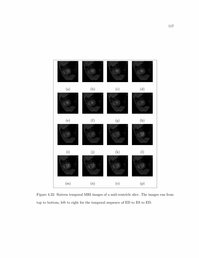
117

(a) (b) (c) (d)

(e) (f) (g) (h)

(i) (j) (k) (l)

(m) (n) (o) (p)

Figure 4.22: Sixteen temporal MRI images of a mid-ventricle slice. The images run from

top to bottom, left to right for the temporal sequence of ED to ES to ED.

118

of the Mayo Clinic.

Sixteen sample spatial slices which cover the left ventricle are shown in Figure

4.23, with the sixteen temporal frames of a mid-ventricle slice shown in Figure 4.24.

Again, the spatial slices cover the LV from apex to base, and the temporal frames cover

the cardiac cycle from ED to ES to ED. Examples of DSR markers in the images are

shown in Figure 4.25, with an endocardial marker on the left and an epicardial marker

on the right. Figure 4.26 shows the dense endocardial displacement vector field from ED

to ES for one DSR dataset. The trajectories are shown against the rendered endocardial

surface at ES.

4.5.3 Motion Validation

In order to validate the motion trajectories formed from the shape-based tracking al-

gorithm, the gold standard marker trajectories and the shape-based, algorithm-derived

point trajectories are compared across the acute dog studies (8 MRI and 4 DSR). To

avoid the possible distortion of the boundary surfaces by the implanted markers which

may cause false shape features, the image intensity around each marker is retouched by a

cardiologist after the markers’ positions have been detected. This procedure is performed

before the contour segmentation process.

Since the position of each marker is the 3D centroid of a cluster of candidate

points in the image, the markers are usually not exactly on the myocardial surfaces. For

both MRI and DSR studies, the point which is the nearest surface point to each marker

is chosen as the surface marker point for the given physical marker. After offsetting the

initial positional difference, the algorithm-derived trajectory of this surface marker point

is considered as the algorithm-derived trajectory of the physical marker. Then, point-by-

point positional errors between the algorithm and gold standard trajectories are compiled

119

(a) (b) (c) (d)

(e) (f) (g) (h)

(i) (j) (k) (l)

(m) (n) (o) (p)

Figure 4.23: Sixteen spatial DSR images which cover the left ventricle. The images run

from top to bottom, left to right to cover the LV from apex to base.

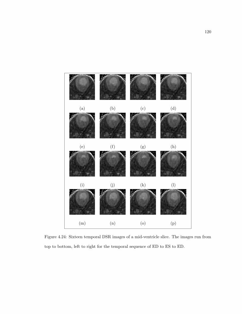
120

(a) (b) (c) (d)

(e) (f) (g) (h)

(i) (j) (k) (l)

(m) (n) (o) (p)

Figure 4.24: Sixteen temporal DSR images of a mid-ventricle slice. The images run from

top to bottom, left to right for the temporal sequence of ED to ES to ED.

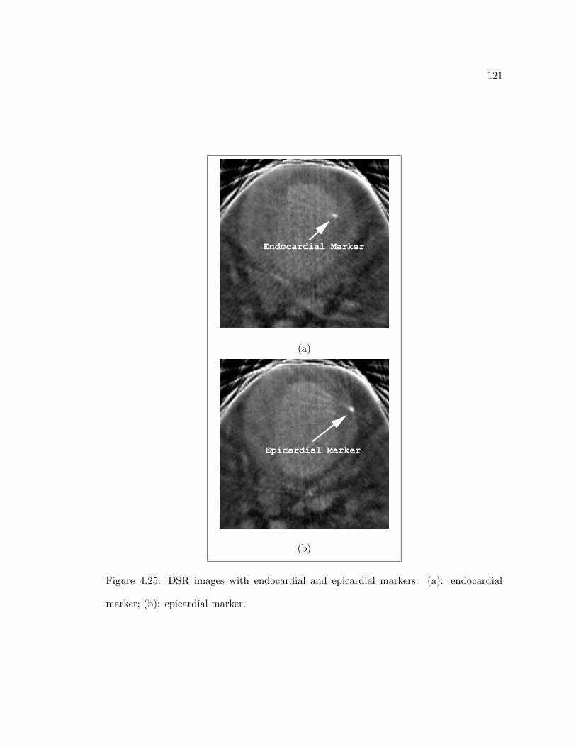
121

Endocardial Marker

(a)

Epicardial Marker

(b)

Figure 4.25: DSR images with endocardial and epicardial markers. (a): endocardial

marker; (b): epicardial marker.

122

Figure 4.26: Dense endocardial displacement vector field from ED to ES for one DSR

dataset. The trajectory arrows are shown against the rendered endocardial surface at ES.

across all 16 time frames for each marker. The mean and the standard deviations of the

positional errors for all the markers are listed in the following tables.

Table 4.3 presents the error analysis for all the markers of both MRI and DSR

data. For the baseline MRI studies, endocardial markers have a mean error of about one

pixel and the epicardial markers have a mean error around two-thirds of a pixel. Since

the endocardial points usually move two-to-three times the distance of the corresponding

epicardial points, this mean error disparity is somewhat expected. However, the endocar-

dial surface often has more shape features than the epicardial surface, which may explain

that both of them have similar error standard deviations.

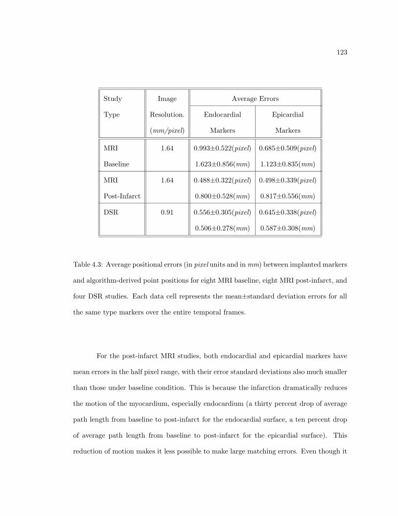
123

Study Image Average Errors

Type Resolution. Endocardial Epicardial

(mm/pixel) Markers Markers

MRI 1.64 0.993±0.522(pixel) 0.685±0.509(pixel)

Baseline 1.623±0.856(mm) 1.123±0.835(mm)

MRI 1.64 0.488±0.322(pixel) 0.498±0.339(pixel)

Post-Infarct 0.800±0.528(mm) 0.817±0.556(mm)

DSR 0.91 0.556±0.305(pixel) 0.645±0.338(pixel)

0.506±0.278(mm) 0.587±0.308(mm)

Table 4.3: Average positional errors (in pixel units and inmm) between implanted markers

and algorithm-derived point positions for eight MRI baseline, eight MRI post-infarct, and

four DSR studies. Each data cell represents the mean±standard deviation errors for all

the same type markers over the entire temporal frames.

For the post-infarct MRI studies, both endocardial and epicardial markers have

mean errors in the half pixel range, with their error standard deviations also much smaller

than those under baseline condition. This is because the infarction dramatically reduces

the motion of the myocardium, especially endocardium (a thirty percent drop of average

path length from baseline to post-infarct for the endocardial surface, a ten percent drop

of average path length from baseline to post-infarct for the epicardial surface). This

reduction of motion makes it less possible to make large matching errors. Even though it

124

still has larger motion, the feature-rich endocardial surface now has similar error statistics

as the epicardial surface.

Since the motion tracking algorithm is based on matching local shape features, it is

not surprising that the higher resolution DSR baseline studies produce better endocardial

tracking results than the MRI studies. The high resolution DSR images pick up more local

detail of the endocardium, thus have smaller mean errors as validated by the markers.

Meanwhile, the accuracy of the relatively feature-less epicardium does not improve, in

terms of pixel units, from the MRI studies, and it is slightly worse than the endocardial

results. Evidently, the rich shape features of the endocardial surface is sufficient to track

the larger motion presented in this case.

Overall, this table illustrates that the trajectories of motion predicted by the

algorithm at points near the implanted markers are very close to the gold-standard motion

of the markers, and are more accurate with better image resolution. Detailed mean error

analysis for each of the MRI and DSR studies are presented in Table 4.4 through Table

4.9.

These error data are also examined as four groups of four time frames in the

cardiac cycle. In this case, the sixteen positional errors of each marker within the cardiac

cycle are sub-grouped into four groups, each with four error measures for each marker.

The mean error and standard deviation of each group are computed to see if there is error

bias over time, and is shown in Table 4.10 for all the studies. For MRI studies, the errors

of the first group, measuring the errors of the first four matches, are generally smaller than

the other three groups which are very similar among themselves. This may suggest that

the algorithm-matched points often drift away from the real marker positions during the

time period of the second group but not any further during later time frames. The baseline

125

MRI Baseline Endocardial Markers

Study 1 2 3 4

EB 0.892±0.376 1.472±0.354 0.983±0.460 1.348±0.433

FB 1.010±0.495 1.266±0.570 1.021±0.381 0.638±0.262

GB 0.165±0.091 0.447±0.189 * 0.704±0.255

HB 1.439±0.111 1.363±0.115 * 1.148±0.610

IB * * 1.405±0.642 *

JB 1.335±0.280 1.088±0.481 * 0.472±0.034

KB 0.505±0.288 * 0.729±0.305 1.178±0.294

LB 1.296±0.265 0.966±0.667 1.004±0.381 0.957±0.437

Table 4.4: Absolute positional errors (in pixels) between implanted endocardial markers

and algorithm-derived point positions for eight canine MRI studies observed under base-

line conditions. Each data cell represents the mean±standard deviation differences found

over sixteen temporal frames for each of the four markers. * denotes that the implanted

marker could not be found in all the temporal frames.

126

MRI Baseline Epicardial Markers

Study 1 2 3 4

EB 0.093±0.015 0.725±0.411 1.776±0.383 0.879±0.284

FB 0.758±0.419 0.836±0.488 0.694±0.179 0.464±0.200

GB 0.183±0.146 1.359±0.280 0.158±0.129 1.150±0.383

HB 0.212±0.139 0.108±0.109 * 0.517±0.146

IB 0.599±0.229 0.422±0.091 0.330±0.083 0.765±0.338

JB 0.293±0.141 * * 1.062±0.255

KB 0.508±0.134 0.636±0.233 0.819±0.550 1.056±0.374

LB 0.480±0.258 1.444±0.240 0.192±0.097 1.337±0.134

Table 4.5: Absolute positional errors (in pixels) between implanted epicardial markers and

algorithm-derived point positions for eight canine MRI studies observed under baseline

conditions. Each data cell represents the mean±standard deviation differences found

over sixteen temporal frames for each of the four markers. * denotes that the implanted

marker could not be found in all the temporal frames.

127

MRI Post-Infarct Endocardial Markers

Study 1 2 3 4

EI 0.161±0.082 0.347±0.143 0.594±0.257 0.251±0.133

FI 0.448±0.373 0.494±0.272 0.458±0.205 0.073±0.046

GI 0.427±0.331 0.764±0.210 0.444±0.126 1.078±0.092

HI 0.365±0.340 0.571±0.245 * 0.461±0.084

II 0.449±0.292 * * *

JI 0.531±0.243 1.007±0.217 * 0.512±0.278

KI 0.829±0.154 * 0.517±0.194 0.643±0.177

LI 0.295±0.164 0.163±0.205 0.390±0.241 0.477±0.227

Table 4.6: Absolute positional errors (in pixels) between implanted endocardial markers

and algorithm-derived point positions for eight canine MRI studies observed under post-

infarct conditions. Each data cell represents the mean±standard deviation differences

found over sixteen temporal frames for each of the four markers. * denotes that the

implanted marker could not be found in all the temporal frames.

128

MRI Post-Infarct Epicardial Markers

Study 1 2 3 4

EI 0.450±0.156 * 0.151±0.131 0.542±0.304

FI 0.071±0.044 0/794±0.250 0.426±0.154 0.417±0.174

GI 0.233±0.269 0.515±0.363 0.352±0.220 *

HI * * * *

II 0.661±0.211 * 0.407±0.332 0.531±0.187

JI 1.284±0.222 * * 0.495±0.222

KI 0.439±0.360 * * 0.593±0.123

LI 0.787±0.161 0.336±0.178 0.426±0.289 0.557±0.269

Table 4.7: Absolute positional errors (in pixels) between implanted epicardial markers

and algorithm-derived point positions for eight canine MRI studies observed under post-

infarct conditions. Each data cell represents the mean±standard deviation differences

found over sixteen temporal frames for each of the four markers. * denotes that the

implanted marker could not be found in all the temporal frames.

129

DSR Endocardial Markers

Study 1 2 3 4

e146 0.331±0.160 0.531±0.117 0.858±0.232 0.941±0.332

e147 0.918±0.152 0.220±0.102 0.616±0.305 0.534±0.119

e181 0.219±0.099 0.404±0.125 0.518±0.334 *

c911 0.744±0.111 0.613±0.244 0.325±0.206 0.569±0.185

Table 4.8: Absolute positional errors (in pixels) between implanted endocardial markers

and algorithm-derived point positions for four canine DSR studies observed under normal

conditions. Each data cell represents the mean±standard deviation differences found over

sixteen to eighteen temporal frames depending on the studies for each of the four markers.

* denotes that the implanted marker could not be found in all the temporal frames.

endocardial markers have the largest increase of errors between the first group and the

next three groups, which may be explained by the larger motion and deformation these

markers undergo to cause mismatches. For DSR studies, the endocardial markers has

consistently small errors over time. Once again, this suggests that the higher resolution,

feature-rich DSR endocardial surface not only produces more accurate matches but also

does so very consistently. The errors of DSR epicardial surfaces have similar patterns as

the MRI ones.

Finally, a visual illustration of the marker position comparison for one MRI base-

line study is shown in Figure 4.27. Here, the real physical marker (green) trajectory and

130

DSR Epicardial Markers

Study 1 2 3 4

e146 0.605±0.332 0.698±0.356 0.682±0.231 0.745±0.238

e147 1.103±0.355 0.406±0.095 0.383±0.122 0.522±0.456

e181 0.291±0.062 0.595±0.256 0.915±0.206 0.504±0.347

c911 0.853±0.372 0.567±0.255 0.782±0.215 0.769±0.133

Table 4.9: Absolute positional errors (in pixels) between implanted epicardial markers

and algorithm-derived point positions for four canine DSR studies observed under normal

conditions. Each data cell represents the mean±standard deviation differences found over

sixteen to eighteen temporal frames depending on the studies for each of the four markers.

surface marker trajectory (blue), both from ED to ES, are plotted together, against the

endocardial surface at ES. Similar figures for one DSR study are shown in Figure 4.28.

From these figures, it is once again evident that the algorithm trajectories are usually

very close to the corresponding marker trajectories.

4.5.4 Injury Validation

For five MRI studies under both baseline and post-infarct conditions, two in vivomeasures

(path length and wall thickening) computed from the algorithm-derived trajectories are

used to evaluate how well the shape-based motion tracking approach can distinguish and

predict myocardial regional injury.

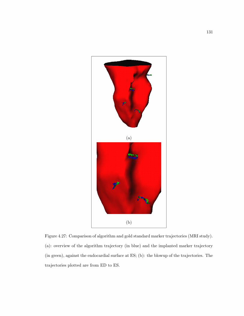
131

(a)

(b)

Figure 4.27: Comparison of algorithm and gold standard marker trajectories (MRI study).

(a): overview of the algorithm trajectory (in blue) and the implanted marker trajectory

(in green), against the endocardial surface at ES; (b): the blowup of the trajectories. The

trajectories plotted are from ED to ES.

132

(a)

(b)

Figure 4.28: Comparison of algorithm and gold standard marker trajectories (DSR study).

(a): overview of the algorithm trajectory (in blue) and the implanted marker trajectory

(in green), against the endocardial surface at ES; (b): the blowup of the trajectories. The

trajectories plotted are from ED to ES.

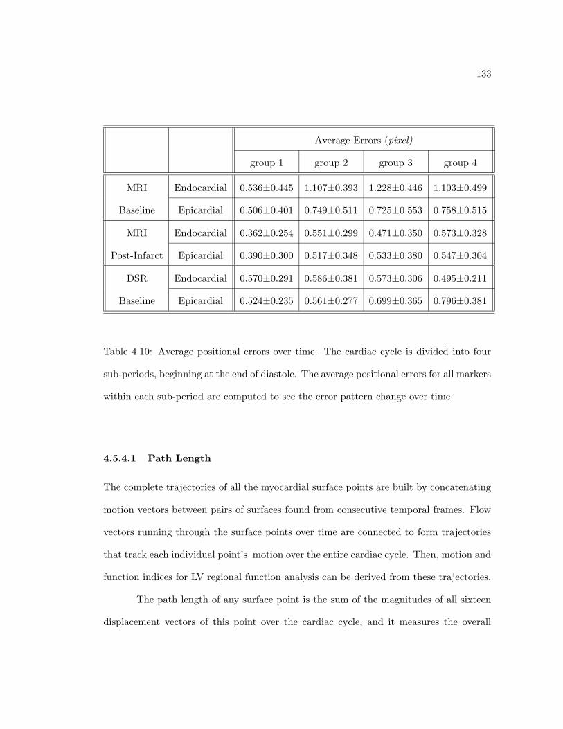
133

Average Errors (pixel)

group 1 group 2 group 3 group 4

MRI Endocardial 0.536±0.445 1.107±0.393 1.228±0.446 1.103±0.499

Baseline Epicardial 0.506±0.401 0.749±0.511 0.725±0.553 0.758±0.515

MRI Endocardial 0.362±0.254 0.551±0.299 0.471±0.350 0.573±0.328

Post-Infarct Epicardial 0.390±0.300 0.517±0.348 0.533±0.380 0.547±0.304

DSR Endocardial 0.570±0.291 0.586±0.381 0.573±0.306 0.495±0.211

Baseline Epicardial 0.524±0.235 0.561±0.277 0.699±0.365 0.796±0.381

Table 4.10: Average positional errors over time. The cardiac cycle is divided into four

sub-periods, beginning at the end of diastole. The average positional errors for all markers

within each sub-period are computed to see the error pattern change over time.

4.5.4.1 Path Length

The complete trajectories of all the myocardial surface points are built by concatenating

motion vectors between pairs of surfaces found from consecutive temporal frames. Flow

vectors running through the surface points over time are connected to form trajectories

that track each individual point’s motion over the entire cardiac cycle. Then, motion and

function indices for LV regional function analysis can be derived from these trajectories.

The path length of any surface point is the sum of the magnitudes of all sixteen

displacement vectors of this point over the cardiac cycle, and it measures the overall

134

motion of the point. One physiological hypothesis of myocardial injury is that the post-

infarct heart will have dramatically decreased motion in the injured zone from its baseline

condition. Hence, it is reasonable to expect that we can measure myocardial regional

injury from the comparison of the baseline and post-infarct path length maps of the

myocardial surfaces.

Examples of endocardial surface path length maps are shown in Figure 4.29 for

both baseline and post-infarct data, with the color scale representing the magnitude of

the shape-tracked pixel-wise movement in pixel units. Here, the “O” sign denotes the

site of the coronary occlusion, and the “I” sign denotes the central infarct zone predicted

by a cardiologist. It is expected from the canine model that the surface region directly

below the coronary occlusion site would be the infarct zone, and thus would have reduced

motion as compared to the baseline data. Visually, it is obvious that the vast region

below the occlusion site in the post-infarct path length map has very little motion.

These two surfaces, the baseline surface and the post-infarct surface at ED, are

registered to each other by minimum distance mapping. The percentage change in path

length for each point from baseline to post-infarct conditions is mapped onto the post-

infarct surface, and is shown in Figure 4.30. Here, the unit of the color scale is percentage,

with the positive values meaning increased path lengths and the negative values meaning

decreased path lengths. As expected from the animal surgical model, the motion of the

surface points under the coronary occlusion site is reduced by at least thirty percent.

In addition, the map follows the expected pattern that while the motion of the central

infarct zone has the largest decrease, the further away a point is from the central zone

the smaller is its motion decrease.

Two validation tests are performed on the path length data. The first test ver-

135

(b)

(a)

0 10 20

(c)

I

I

O

O

Figure 4.29: Baseline and post-infarct endocardial path length maps. (a): baseline path

length map; (b): post-infarct path length map; (c): color scale (in pixel units). The

“O” sign denotes the site of the coronary occlusion, and the “I” sign denotes the central

infarct zone predicted by a cardiologist.

136

(b)

(a)

−60 −45 −30 0 30 45 60

I

O

Figure 4.30: Change in endocardial path length from baseline to post-infarct condition.

(a): map of percentage change of path length; (b): color scale (in percent), positive values

mean increased path lengths and the negative values mean decreased path lengths). The

“O” sign denotes the site of coronary occlusion, and the “I” sign denotes the central

infarct zone predicted by a cardiologist.

137

Path a Factor a b axb

Length Infarct Zone Normal Zone F p F p F p

b Baseline 22.1± 3.8 21.7± 3.5 3.46 0.14 4.50 0.10 10.44 0.03

Factor Post-Infarct 11.0± 7.7 19.9± 4.5

Table 4.11: Table of means and standard deviations of algorithm-derived in vivo path

length measures (in mm), observed in the infarct zone and in a remote normal zone for

five acute canine studies under both baseline and post-infarct conditions.

ifies the validity of using path length changes to differentiate the normal zone and the

infarct zone motion behavior. For both the baseline and the post-infarct data of five

MRI studies, the mean and standard deviation of the path lengths are computed for the

antero-apical infarct zone and the remote normal zone from sampled points near the two

implanted markers. These data are shown in Table 4.11. Two-way analysis of variance is

performed for the path length measure, and the F-statistics and p values are computed for

comparisons between a) baseline and post-infarct conditions, b) infarct zone and normal

zone, and the interaction of a) and b). As can be seen in the table, the path length mea-

sure shows significant differences in the interaction term, indicating that the algorithm

can discriminate the infarction and differentiate the normal zone and infarct zone. More

detailed testing showed that the significance of the interaction is due to the difference

of the measures in the infarct zone at baseline and post-infarct conditions (p < 0.028),

and the difference between the infarct zone and the normal zone at post-infarct condition

(p < 0.022).

138

The second test verifies the algorithm-predicted extent (area) of the infarct zone

on the endocardial surface against other standard forms of myocardial regional viability

measurement. Three-dimensional post mortem endocardial injury zones are found by dig-

itizing color photographs of TTC-stained post mortem myocardium slices (5mm thick) of

the excised hearts. The experiments were performed by Dr. Albert Sinusas of Yale med-

ical school. The endocardial, epicardial and infarct zone boundaries of the post mortem

left ventricle are hand-traced and stacked to reconstruct the LV volume representation.

Figure 4.31 shows one 2D frame of the color photograph, the rendered LV volume (epi-

cardial surface in transparent green, endocardial surface in red, and the infarct zone in

blue), and the rendered endocardial surface along with the endocardial infarct zone. The

areas of the endocardial infarct zones are computed and compared to the areas defined

by thresholding the magnitudes of the in vivo algorithm-derived path length measures.

Within a search window defined by a sphere centered at the central infarct marker I with

radius being the distance between I and the occlusion marker O, points are considered

to be inside the infarct zone if their post-infarct path length fell to levels below 80%

of the mean infarct zone baseline value, computed from sample points near the infarct

zone marker. The mean and standard deviation of both post mortem and in vivo infarct

areas are reported in Table 4.12, as is their Pearson product-moment correlation. The

high correlation value points to the utility of these measures for measuring the extent of

endocardial injury.

Another form of myocardial regional viability measurement is Single Photon Emis-

sion Computed Tomography (SPECT), which measures myocardial blood flow and thus

indicates tissue viability. Figure 4.32 shows an example of mapping the SPECT counts,

of the same study as that in Figure 4.30 and 4.31, onto the MRI derived endocardial

139

(a)

EpicardialSurface

EndocardialSurface

Injury Zone

(b)

I

O

(c)

Figure 4.31: Post Mortem injury found from TTC staining. (a): 2D color photograph

of TTC stained myocardial slice, with the injury region delineated by a green line; (b):

rendered LV volume reconstructed from digitized and segmented 2D post mortem slices;

(c): rendered endocardial surface along with the endocardial infarct zone (scaled to the

same size as the path length map of Figure 4.30). The epicardial surface is in transparent

green, the endocardial surface is in red, and the infarct zone is in blue.

140

Infarct Area (mm2)

Study 1 2 3 4 5 average Correlation

Post Mortem 963 811 833 749 623 796±124 0.968

In Vivo 939 855 807 710 602 783±131

Table 4.12: Correlation between post mortem and in vivo infarct areas.

surface. Since surface points with SPECT counts under sixty percent are usually consid-

ered to be injury points, we can again compare the SPECT and path-length infarct areas

to validate the ability of our shape-based motion tracking approach in predicting the

extent of myocardial injury. (We should note that SPECT over-estimates low flow while

it under-estimates high flow, thus often under-estimating the extent of injury region.)

4.5.4.2 Wall Thickening

In the previous section, we have shown that the algorithm-derived path length changes

of the myocardial surface points predict the existence and extent of the infarct zone.

However, the path length measure is a gross overall measure of local deformation and

global motion, which may result in under-estimation of the injury. This is because the

global motion of the injury zone does not decrease dramatically due the coupling between

myocardial tissues. Meanwhile, myocardial thickening, measured by the change of thick-

ness of LV wall between ED and ES, may provide additional insight into the myocardium

viability since it is a more local measure similar to radial strain. For every epicardial

141

I

O

30 45 60 80 90 95

Figure 4.32: Myocardial injury zone from SPECT counts. (a): map of SPECT counts

onto the MRI derived endocardial surface; (b): color scale (in percent), region with counts

under sixty percent is often considered to be injury zone.

point, its thickening measure is defined as:

τ ′ =τED − τES

τED(4.66)

where τED and τED are the thickness of the LV wall at ED and ES. The thickness of

the wall is computed by emitting a ray from the epicardial point in its inward normal

direction until it intersects the endocardial surface, and the distance between the inter-

section and the epicardial point is considered to be the wall thickness. Thickening is a

gross approximation to the radial strain of the wall.

142

Thickening a Factor a b axb

Measure(τ ′) Infarct Zone Normal Zone F p F p F p

b Baseline 44.6± 26.2 34.7± 19.5 0.82 0.42 4.90 0.09 44.7 0.003

Factor Post-Infarct 6.1± 13.2 37.4± 13.4

Table 4.13: Table of means and standard deviations of algorithm-derived in vivo measure

of radial thickness change (in percentage), observed in the infarct zone and in a remote

normal zone for five acute canine studies under both baseline and post-infarct conditions.

Again, for both the baseline and the post infarct data of five MRI studies, the mean

and standard deviation of the thickening measures are computed for the antero-apical

infarct zone and the remote normal zone from sampled points near the two implanted

markers. The data are shown in Table 4.13. Two-way analysis of variance is again

performed for the change of thickening measure, and the F-statistics and p values are

computed for comparisons between a) baseline and post-infarct conditions, b) infarct

zone and normal zone, and the interaction of a) and b). As can be seen in the table,

the thickening measure shows significant differences in the interaction term, indicating

that the algorithm can distinguish infarction. More detailed testing showed that the

significance of the interaction is due to the difference of the measure in the infarct zone at

baseline and post-infarct conditions (p < 0.010), and the difference between the infarct

zone and the normal zone at post-infarct conditions (p < 0.045). This shows the validity

of using our algorithm-derived, point-tracked LV wall thickening measure to differentiate

the normal zone and the infarct zone motion behavior.

143

4.6 Conclusion

A shape-based motion tracking approach has been developed in this chapter. It is our

hypothesis that we can use the shape properties of the myocardial surfaces to track the

motion trajectories of a dense field of points over the entire cardiac cycle, which can then

be used to predict the existence and extent of myocardial injury.

Locally coherent surface representation is achieved by non-shrinkage Gaussian

smoothing of the Delaunay triangulated surface, weighted by the natural coordinates of

each surface point. The smoothed surface is characterized by its differential geometric

properties through multi-order local surface fit, again using the natural neighbor rela-

tionships defined from the Delaunay triangulation. Surface points on successive temporal

frames are matched based on differential geometric features and an ideal-thin-plate bend-

ing model of local surface patches. The optimal dense motion field is obtained using a

mathematical optimization strategy to combine the data-derived initial matching infor-

mation with a locally coherent smoothness model.

Experiments are been performed on eight MRI canine studies under both baseline

and post-infarct conditions, and on four DSR canine baseline studies. The accuracy of the

algorithm point tracking results has been validated against the gold-standard motion of

the implanted imaging-opaque markers. The changes in motion parameters, path length

and wall thickening measures, between baseline and post-infarct data are quantified to

assess myocardial viability, and are validated using cardiac perfusion data.

Chapter 5

Volumetric Deformation Analysis

5.1 Introduction

In the previous chapter, we proposed a shape-based approach for computing point-wise

myocardial surface motion fields between successive image frames. Even though purely

surface motion characteristics, such as path length and displacements, do indicate the

location and extent of injury reflected on the endocardial and epicardial surfaces, the

most robust description of functional abnormalities of the myocardial wall should include

measurement of the entire transmural motion and deformation of the myocardium. This

is important, in part, in order to assess the transmural extent of myocardial injury which

can be related to patient prognosis. Despite a number of recent attempts in the literature,

it is not yet the case that transmural deformation of the complete LV can be accurately

and reproducibly quantified in three dimensions over time. One critical limitation to the

successful quantification of this information is the fact that the appropriate computa-

tional framework has not yet been developed for assembling the complex cues related to

LV deformation that are available from image data sets. Furthermore, instead of using

144

145

proper biomechanical constraints of the myocardium to guide the motion and deforma-

tion recovery process, only empirical models have been employed to analyze the image

data.

We propose here an integrated framework for the analysis of left ventricular mo-

tion and deformation. This unified approach is based upon the use of image analysis

strategies and biomechanical modelling, and is embedded in a finite element framework

for the integration of disparate sources of displacement and velocity information, hereto-

fore used only separately, to help guide volumetric motion and deformation analysis. In

this manner, noisy and complementary image information can be jointly utilized from

both the LV epicardial and endocardial boundaries (where the shape-based estimated

displacements are reliable) and the mid-wall (where measures such as MR phase velocity,

MR tagging, and echocardiographic Doppler are reliable). In addition, the continuum

mechanical properties of the myocardium provide physically meaningful constraints on

the dynamic behaviors of the LV tissue. This, along with the finite element framework,

enable us to incorporate naturally actual known cardiac physical parameters, such as

pressures, into the motion/deformation estimation system.

5.2 Image-Derived Information

It is the goal of the unified motion and deformation analysis framework to characterize

more completely the transmural function of the left ventricle. It takes advantage of the

availability of several complementary image sources of LV anatomy and motion (displace-

ment and velocity) information to quantify the dynamic behavior of the myocardium. In

this section, we will briefly discuss several of the image sources which have been, or can be,

used in our framework. Because of image availability, the remaining sections of this chap-

146

ter will focus on estimating motion and deformation by integrating shape-based boundary

displacement and phase contrast velocity information from MR images. We should point

out, however, that our unified framework can also use data from other imaging modalities

include MR tagging, DSR, and echocardiography.

5.2.1 Shape-Based Boundary Displacement

As described in detail in the previous chapter, we have proposed that we can use the

shape properties of the endocardial and epicardial surfaces to track the motion of a

dense field of surface sample points over the entire cardiac cycle. This motion tracking

method is based on locating and matching differential geometric landmarks and using a

mathematical optimization reasoning strategy to combine a locally coherent smoothness

model with data-derived information to obtain dense field motion vectors.

We will use these boundary displacement vectors as the shape-derived bound-

ary information in our integrated framework. For computational stability and for not

over constraining the boundary motion by shape information, however, only a subset of

boundary displacement vectors in which we have the highest confidence will be used in

the integrated estimation process. This subset of displacement vectors is often comprised

of the vectors that begin from landmarks of the first surface or terminate at landmarks

of the second surface. We will use this subset of boundary displacement vectors as the

shape-derived boundary information in our integrated framework, and denote these dis-

placement vectors as Uboundary.

5.2.2 MR Phase Contrast Images and Mid-Wall Instantaneous Velocity

As discussed in Chapter 2, a new imaging technique[99, 98], Phase Velocity Magnetic

Resonance Imaging recently, has been developed. It incorporates velocity phase encoding

147

into a conventional cine-MR sequence and produces images of myocardial instantaneous

velocity throughout the cardiac cycle. Phase contrast methods can depict motion param-

eters with pixel precision and thus provide a high resolution technique for quantitative

measurements[24].

The MR phase contrast velocity technique relies on the fact that a uniform motion

of tissue in the presence of a magnetic field gradient produces a change in the MR signal

phase, φ, that is proportional to its velocity[98]:

φ = νγM1 = νγ

∫ TE

0G(t)t dt (5.1)

where G(t) is the gradient strength as a function of time (the gradient waveform), ν the

tissue velocity, M1 the first moment of the gradient waveform, TE the echo delay time,

and γ the gyromagnetic ratio. The gradient waveform can be modified to alter the first

moment (motion sensitivity) while maintaining the same image localization characteris-

tics. Images acquired with this altered waveform will have a different phase shift due to

motion. The velocity in a particular spatial direction can be estimated by measuring the

difference in phase shift between two acquisitions with different first gradient moments.

Hence, instantaneous velocity maps encoded for motion in all three spatial dimensions

may easily be obtained at multiple time instances throughout the cardiac cycle using a

phase contrast cine-MR imaging sequence. The acquired velocity maps may then be used

to provide information on tissue displacement, strain, strain rate, and other quantitative

measures of motion and deformation. Figure 5.1 shows examples of phase contrast im-

ages of a canine mid-ventricle slice. In this dataset, three contiguous short axis slices were

collected using the cine phase contrast gradient echo sequence. The imaging parameters

148

were: flip angle = 30, TE = 34msec, TR = 34msec, FOV = 28cm, 5mm skip 0, matrix

256x128, 4 nex, venc = 15cm/sec. It is important to note that the magnitude image and

the three directional velocity images are perfectly registered since they are acquired from

the same complex MR signal.

In theory, instantaneous velocity can be derived for each pixel in each image ac-

quisition to provide a complete description of instantaneous movement of the LV at that

moment. However, the phase contrast velocity estimates at interfaces between structures,

e.g. near the endocardial and epicardial boundaries, are extremely noisy. It is difficult

to obtain low noise estimates of velocity at the boundaries since some spatial averaging

must occur, and thus pixels outside the myocardial wall (the blood pool for the endo-

cardium and the air or other tissues for the epicardium) are sometimes included for the

velocity estimates of the myocardial points. Thus, phase contrast images only provide

reliable instantaneous motion information for the mid-wall region of the LV but not at

the myocardial boundaries.

Since the velocity maps themselves only provide instantaneous motion informa-

tion, efforts have been made to estimate the displacement and other measures to assess the

motion and deformation of the myocardium[24, 75, 81, 96, 98, 97]. Assuming some con-

stant velocity conditions between time frames, these approaches often use forward and/or

backward integration of the velocity to track each point and estimate the displacement

vector over time. More recently, a framework combining a spatially regularized velocity

field with temporal Kalman filtering has been proposed to characterize the deforming LV

in 2D[75], which takes into account the uncertainties in the velocity measurement near

the boundaries.

We believe, however, that the weaknesses of the phase velocity image data, such

149

(a) (b)

(c) (d)

Figure 5.1: Phase contrast MR images. (a): the magnitude image; (b): the x direction

velocity image; (c): the y direction velocity image; (d): the z direction velocity image.

Please note that the velocity images show both positive and negative values of the velocity,

with the dark colors representing negative values, the neutral grey for no motion, and

bright colors for positive velocity values.

150

as noisy boundary data and uncertainty about point correspondences (constant velocity

conditions between temporal frames are often assumed to compute displacements), makes

it very difficult to obtain a reliable and robust assessment of myocardial motion and

deformation over the entire LV and through the cardiac cycle using the data alone. It is

more appropriate to use phase velocity information as only one source of data constraints

within an integration framework, where it can be utilized without gross assumptions about

the velocity conditions between temporal frames. Furthermore, since the phase image is

derived from the same complex magnetic resonance signal as the regular magnitude MR

image data upon which the shape-based boundary motion algorithm is based, these two

image data are perfectly registered and can be used synergistically. In summary, we will

use the reliable mid-wall MR phase velocity data as the mid-wall image information in

our integrated framework, and we denote these mid-wall velocity vectors as Umid−wall.

5.2.3 Other Image-Derived Data

5.2.3.1 MR Tagging and Tag Displacement

A review of MR tagging technique and tagged image based approaches of analyzing

myocardial motion and deformation has been given in the Chapter 2. Here, we want to

point out that the sparse MR tag displacement information can be easily incorporated

into our integrated approach. If the MR tagging image can be derived from the same

MR signal as the regular MR image and the phase contrast image, which is technically

feasible, we can treat the tag displacement in the same way as the shape-based boundary

displacement in the integration process, although these tag displacements can be for

mid-wall points and/or boundary points. The integration results would be the optimal

compromise between three complementary imaging data sources.

151

5.2.3.2 DSR Image and Optical Flow

The Dynamic Spatial Reconstructor, a three-dimensional computerized tomography scan-

ner, provides high resolution, real-time images of the beating heart [104, 106]. We have

applied and validated our shape-based boundary motion tracking algorithm on canine

DSR data.

Even though the DSR does not directly provide tissue velocity or other motion

information, we do note that velocities (optical flow) can be estimated from the spatio-

temporal changes of the image intensity values[122]. Even though optical flow in general

is not a good measurement for estimation cardiac motion, the estimated velocities should

be fairly reliable for high resolution (both spatially and temporally), high quality image

data such as DSR[75].

The integration of the shape-based boundary displacement and optical flow-based

velocity would effectively use both image boundary information and grey level intensity

information, which have only been used separately before.

5.2.3.3 Echocardiography and Doppler Velocity

There is a fairly long history of efforts aimed at trying to use echocardiographic infor-

mation for quantitative analysis of the left ventricle, often aimed at extracting global

parameters such as volume or volume differences (e.g. stroke volume and/or ejection

fraction) [66, 119]. Historically, there have been few efforts that have been aimed at

quantifying 3D motion and deformation. However, we note the work of McPherson[73]

in the LV and, more recently, the interesting work of O’Donnell[86] and Raghavan[102]

who are all exploring the use of ultrasound to measure strain and tissue elasticity.

Even though echocardiographic data often have low resolution, we believe that our

152

shape-based motion tracking approach would still be able to estimate the gross motion

behavior of the LV boundary from these images. Furthermore, the use of color Doppler

imaging of the velocities related to the movement of myocardial tissue fits nicely within

our unified framework. Doppler imaging basically uses low pass filtering to extract in-

formation related to the lower frequency tissue motion, instead of the higher frequencies

typically utilized when visualizing flow patterns in vessels or within the LV cavity. While

only one component of the tissue velocity is available (orthogonal to the probe), this is

nonetheless dense field information that is useful in our proposed integrated scheme.

The echocardiography based LV motion and deformation analysis will be unde-

niably very crude. However, we think it provides a relatively less expensive procedure to

assess the state of health of the heart.

5.3 Continuum Mechanical Models

In this section, we discuss some of the basic concepts of continuum mechanics (see

Fung[38] and Spencer[123] for more detail) and the models of myocardium based on

these ideas[57, 59, 71, 84, 121]. It should be pointed out that our purpose is not to

establish sophisticated constitutive models which best describe the mechanical proper-

ties of the myocardium. Instead, the emphasis is on using practical yet realistic models

of the myocardium including relationships between the strain and stress, to guide the

integrated framework to recover the motion and deformation of the LV from multiple,

complementary image data.

153

5.3.1 Continuum Mechanics

Continuum mechanics deals with the mechanical behaviors of materials under the action

of applied force, where the materials are continuous (or at least piecewise continuous) and

deformable[38, 123]. The results of applying forces are often found in the changes of the

kinematic variables such as displacement, velocity and acceleration fields of the object:

each point moves a certain distance at a certain velocity and acceleration, each of which

is dependent on both the point’s position and the mechanical properties of the object.

5.3.1.1 Deformation Measure

A given particle of the object may be distinguished by its coordinates X = (X1, X2, X3)

at the undeformed state (t = 0). Thus the coordinates X serve as labels with which to

identify the particles of the object, and is called the material coordinates. Denoting the

corresponding coordinates (the spatial coordinates) of the same particle at the deformed

state (at time t) to be x = (x1, x2, x3), then the equation

x = x(X, t) (5.2)

describes a motion of the body which gives the position of each particle at time t. Further-

more, the deformation gradient tensor F relates the deformed and undeformed particle,

and its nine components are defined as:

FiR =∂xi∂XR

i, R = 1, 2, 3. (5.3)

154

In general, F is not a symmetric tensor. Furthermore, although F is important in the

analysis of deformation, it is not itself a suitable measure of deformation. This is because

a measure of deformation should have the property that it does not change when no

deformation takes place; therefore it must be unchanged in a rigid-body motion. F does

not have this property; in fact in rigid-body motion, x = Q(t)X+ c(t), F is equal to the

rotation matrix Q. However, if there is only translation in the rigid-body motion, F is

equal to zero.

Hence, the Lagrangian strain tensor E is defined:

E =1

2(FTF− I) (5.4)

where I is identity matrix. It is a suitable measure of deformation since it reduces to

the zero tensor when there is only rigid-body motion. If the deformation of the object is

described by Equation 5.2 which gives the dependence of x onX, then it is straightforward

to calculate the nine components of E:

ERS =1

2(FiRFiS − δRS) =

1

2(∂xi∂XR

∂xi∂XS

− δRS), i, R, S = 1, 2, 3. (5.5)

where δRS is the Kronecker delta. This Lagrangian strain tensor E has three invariants,

the three principal strain invariants. Associated with the principal strains, the eigenvalues

of E, there also exist three principal strain directions, the corresponding eigenvectors. The

principal strains and their directions are intrinsic to a given state of deformation.

The above definitions are valid in any arbitrary coordinate systems. In Cartesian

coordinate system of (x, y, z) with displacement vector in the form of [u(x, y, z)]T =

(x − X) = (u(x, y, z), v(x, y, z), w(x, y, z)), the Lagrangian strain tensor reduces to the

155

simple form:

Exx =∂u

∂x+

1

2

[

(∂u

∂x)2 + (

∂v

∂x)2 + (

∂w

∂x)2]

(5.6)

Eyy =∂v

∂y+

1

2

[

(∂u

∂y)2 + (

∂v

∂y)2 + (

∂w

∂y)2]

(5.7)

Ezz =∂w

∂z+

1

2

[

(∂u

∂z)2 + (

∂v

∂z)2 + (

∂w

∂z)2]

(5.8)

Exy =1

2

[

∂u

∂y+∂v

∂x+ (

∂u

∂x

∂u

∂y+∂v

∂x

∂v

∂y+∂w

∂x

∂w

∂y)

]

(5.9)

Eyz =1

2

[

∂v

∂z+∂w

∂y+ (

∂u

∂y

∂u

∂z+∂v

∂y

∂v

∂z+∂w

∂y

∂w

∂z)

]

(5.10)

Ezx =1

2

[

∂w

∂x+∂u

∂z+ (

∂u

∂z

∂u

∂x+∂v

∂z

∂v

∂x+∂w

∂z

∂w

∂x)

]

(5.11)

In small deformation condition, if the components of the displacement are such that their

first derivatives are so small that the squares and products of the partial derivatives are

negligible, the Lagrangian strain tensor reduces to the infinitesimal strain tensor [ε]:

[ε] =

εxx

εyy

εzz

εxy

εyz

εzx

=

∂∂x 0 0

0 ∂∂y 0

0 0 ∂∂z

12∂∂y

12∂∂x 0

0 12∂∂z

12∂∂y

12∂∂z 0 1

2∂∂x

u

v

w

= [B′][u] (5.12)

where [B′] is the strain-displacement matrix. For the convenience in further derivations,

[ε] is expressed as a 6x1 vector instead of a 3x3 matrix. From Equation 5.12, it is evident

that the strain tensor of a particle of an object is a function of its displacement vector,

which in turn is a function of the spatial position of the particle.

156

5.3.1.2 Constitutive Equation

The strain measure of an object holds no matter what material the object is made of.

It is insufficient to describe the mechanical behavior of any particular material, which

means that by itself it cannot determine the changes of kinematic variables when forces

are applied, or determine the changes of stress when strain is induced. The constitutive

equations of a material specifies the dependence of the stress in an object on the kinematic

variables such as the strain measure, and vice versa[38, 123].

Following the law of conservation of energy, the material time derivative of the

sum of the kinetic energy and internal energy is equal to the sum of the rate at which

mechanical work is done by the body and surface forces acting on the object and the

rate at which other energy (heat flux, chemical energy, radiation energy, electromagnetic

energy, et al. ) enters the object[123]. If other energy is absent or neglected, then all

the mechanical work done on an object either creates kinetic energy, or is stored as

potential energy (called the strain energy W) which depends only on the deformation.

For a linear elastic material, W may be approximated by a quadratic function of the

infinitesimal strain components. For a general finite elastic deformation, W depends

on an arbitrary manner on the deformation gradient F. The specific manner of this

dependence determines the mechanical behavior of any specific material.

Under the general finite elastic deformation theory[123], the strain-energy function

W (F) of an object depends on the deformation gradient tensor F. While F itself is not

a zero tensor if the object is undergoing rigid-body rotation, there is a restriction on the

value of the strain-energy function such that it is not changed if a rigid-body rotation is

superimposed on the deformation. Suppose that a particle with initial position X moves

to x. Further, a rigid rotation is superimposed on the particle to x = Mx, where M is

157

the rotation matrix. Let

FiR =∂xi∂XR

, FiR =∂xi∂XR

(5.13)

Then

FiR = Mij∂xj∂XR

= MijFjR, or F = MF (5.14)

Thus, we require that

W (F) = W (MF) (5.15)

for all rotation matrices M. A necessary condition for the strain-energy function to

be independent of superimposed rigid motion is that it can be expressed in the form

W (FTF)[123].

In general, the constitutive equations for a finite elastic solid are defined as:

Ti,j =ρ

ρ0FjR

∂W (F)

∂FiRi, j, R = 1, 2, 3. (5.16)

where T is the stress tensor, ρ0 and ρ the initial and final material density respectively.

The equation’s apparent simplicity is deceptive, because W is a function of the nine

components of F, which makes it impractical to perform experiments to determine this

function for any particular elastic material. In practice, various assumptions under dif-

ferent conditions have been made to derive practical yet realistic strain energy functions

of the materials, from which the material constitutive laws can be derived.

158

5.3.2 Models of the Myocardium

The mechanical behavior of the myocardium is very diverse and complex, and it would be

an admirable but extremely difficult goal to formulate its constitutive equations under all

circumstances. Rather, we seek to establish equations which describe the most important

features of the material while retaining physical plausibility. Ideally, the constitutive

equations of the myocardium should characterize the non-linear, anisotropic material

properties of the cardiac muscle in a compact way with as few parameters as possible.

The relationship should also be formulated based on experimental measurements. There

has been a fair amount active research in the biomechanics community in developing

myocardial constitutive laws under different conditions and assumptions[57, 59, 71, 84,

121]. Since the stress tensor can been found from the derivatives of W with respect to

the strain components[60], emphasis has been on the derivation of various strain energy

functions for different myocardial models.

In general, two aspects of the mechanical properties of the myocardium have

been considered: the passive tissue properties and the active muscle tension develop-

ment. A constitutive law for passive tissue properties requires a fully three-dimensional

relationship between the six components of the stress and the six components of the

strain (assuming symmetric material), whereas the active muscle law requires only a one-

dimensional relationship between the fiber strain and the active muscle tension[59]. Since

the purpose of our system is to use the constitutive relationship to help recover motion

and deformation from image data, not to model the forward activation of the left ventri-

cle, we will only discuss the passive constitutive laws from now on. However, we do realize

that the active muscle tension development largely determines the active contraction and

expansion of the myocardium, and incorporating active muscle law into our framework

159

would add important actual physical constraints into the recovery process.

The simplest constitutive relationship is that of the linear elastic solid, or the

Hookean elastic solid. In this case, the strain energy function has the form

W =1

2cijklεijεkl (5.17)

where εij and εkl are components of the infinitesimal strain tensor and cijkl are material

specific elastic constants. Under this model, Equation 5.16 can be simplified to:

σij = cijklεkl (5.18)

where σij is a stress tensor component. This is the constitutive equation for a linear elastic

solid. It is evident that the stress components are linear functions of the infinitesimal

strain components.

Under the assumptions that the strain and stress tensors are symmetric, and the

material is isotropic (the elastic properties are identical in all directions), there are exactly

two elastic constants which characterize the material and Equation 5.17 is further reduced

to:

σij = λδijεkk + 2µεij (5.19)

where constants λ and µ are called the Lame constants.

In Cartesian coordinates, the linear isotropic constitutive law can be written as:

[σ] = [C][ε] = [C][B′][u] (5.20)

160

[ε] = [C]−1[σ] = [D][σ] (5.21)

where [σ] = [σxx σyy σzz σxy σyz σzx]T is the stress vector, [C] is the stress-strain or

material matrix:

[C] =E

(1 + ν)(1− 2ν)

1− ν ν ν 0 0 0

ν 1− ν ν 0 0 0

ν ν 1− ν 0 0 0

0 0 0 1− 2ν 0 0

0 0 0 0 1− 2ν 0

0 0 0 0 0 1− 2ν

(5.22)

and [D] is the strain-stress or compliance matrix:

[D] =1

E

1 −ν −ν 0 0 0

−ν 1 −ν 0 0 0

−ν −ν 1 0 0 0

0 0 0 1 + ν 0 0

0 0 0 0 1 + ν 0

0 0 0 0 0 1 + ν

(5.23)

The Young’s modulus E = µ(3λ+2µ)λ+µ and the Poisson’s ratio ν = λ

2(λ+µ) in the equations are

both material related constants. It should be noted that these linear, isotropic constitutive

equations do not properly describe the mechanical behaviors of the myocardium because

myocardium is non-linear and anisotropic. However, they are very simple to use in a

computational framework, and are often treated as the first order approximations of more

161

sophisticated constitutive laws under small deformation conditions. An experimental

method for evaluating a slightly modified model (isotropic exponential strain energy)

in vivo has been performed on 2D MR tagging data[26]. The overall strategy of this

study is based on the classical approach in which a particular model for the constitutive

relation is fit to a set of experimental data that describe the displacement of the ventricles

during diastolic expansion. The finite element method is used to recover the constitutive

parameters from the pre-calculated 2D deformation derived from MR tagging data.

More sophisticated models of the myocardium often take into account the micro-

structures of the cardiac muscle. The architectures and orientations of the myofibers,

the organization of the myocardial sheets, and the collagen inter-connections between the

micro-structures determine the non-homogeneous and non-linear stress-strain relationship

throughout the myocardium[59, 71]. In one of the attempts to base the constitutive laws

upon the micro-structures of the cardiac muscle, the myocardium is treated as a trans-

versely isotropic material[71]. The constitutive equation for the passive tissue is given by

an exponential strain energy function W (Eij), where Eij are Lagrangian strain compo-

nents referred to the fiber coordinate system (fiber (F ), cross-fiber (C), and transmural

(T) coordinates):

W =1

2c(eQ − 1)−

1

2p(I3 − 1) (5.24)

where c is a constant and

Q = b1E2FF + b2(E

2CC + E2TT + E2CT + E2TC) + b3(E

2FC + E2CF + E2FT + E2TF ) (5.25)

Here, p is the hydrostatic pressure Lagrange multiplier and I3 is the third principal

162

invariant of the strain.

Because the composition of the myocardial tissue is often too complex to derive

constitutive laws from a knowledge of the mechanical properties and layout of the micro-

structural components, simpler empirical relationships were proposed and constitutive

parameters estimated from biaxial testing of the tissue were used. Characteristic fea-

tures of the mechanical properties of passive myocardium include a). the stress-strain

relationships along longitudinal, circumferential, and radial axes of the LV are quite dif-

ferent and nearly independent of each other, and b). the axial stress is very low at low

axial strains but rises rapidly as the strain approaches a characteristic limiting value for

that axis[121]. Based on these observations, a pole-zero strain energy function has been

proposed by Hunter[59]:

W = k1e211

(a1−e11)α1 + k2e222

(a2−e22)α2 + k3e233

(a3−e33)α3

+ k4e212

(a4−e12)α4 + k5e223

(a5−e23)α5 + k6e231

(a6−e31)α6 (5.26)

where eij are the strain components, am are the parameters expressing the limiting values

for a particular type of deformation and are always larger than the corresponding strain

components, αm are the parameters expressing the curvature of the uniaxial stress-strain

curves, and km are parameters giving the relative weighting of each strain energy term.

Similar simplified strain energy functions have been proposed by Humphrey et al.

[57, 84], identified from biaxial tests on non-contracting canine mid-wall tissue:

W = c1(α− 1)2 + c2(α− 1)2 + c3(I1 − 3)

+ c4(I1 − 3)(α− 1) + c5(I1 − 3)2 (5.27)

163

where I1 = tr[FTF], and αm are the stretch ratios at given muscle fiber directions.

While such non-linear models more appropriately describe the complex mechanical

properties of the myocardium, they are often computationally very expensive. In the rest

of this chapter, all the experiments have been conducted using the linear isotropic model,

which is more feasible computationally. However, the different choices for the continuum

models of the myocardium do not change the fundamental underlying concepts of the

integrated framework to recover motion and deformation from image data, although we

realize that more sophisticated non-linear models probably will produce more realistic

and accurate results.

5.4 Finite Element Analysis

The finite element method (FEM) is a numerical analysis technique for obtaining approxi-

mate solutions to a wide variety of engineering problems, especially continuum mechanics

problems[12]. Unlike the commonly used finite difference method, which envisions the

solution region as an array of grid points, the finite element method envisions the solu-

tion region as built up of many small, interconnected subregions or finite elements. Its

basic premise is that a solution region can be analytically modeled or approximated by

replacing it with an assemblage of discrete finite elements, the finite element mesh, which

can represent exceedingly complex shapes. In essence, a complex problem over a large

solution region can be reduced to a series of greatly simplified problems over many finite

elements. The solutions to a series of governing equations of the elements give a piecewise

approximation to the solution of the governing equation of the original system[56]. For

the analysis of left ventricular motion and deformation, the LV (the solution region) is

represented by many small tetrahedra (the finite elements) constructed from the Delaunay

164

triangulation of the sampled points. Also, the displacement-based solutions of the gov-

erning equations give the approximate motion at the sampled points and the deformation

of the elements.

5.4.1 Element and Interpolation Function

In a continuum mechanics problem, the field variable (the displacement in our case)

possesses infinitely many values because it is a function of each generic point in the

solution region. Consequently, the problem is one with an infinite number of unknowns.

The finite element method reduces the problem to one with a finite number of unknowns

by dividing the solution region into elements and by expressing the unknown field variable

in terms of assumed approximating or interpolation functions within each element. These

interpolation functions are defined in terms of the values of the field variable at specified

nodal points (the sampled LV points in our case). The nodal values of the field variable

and the interpolation functions completely define the behavior of the field variable within

the element. In general, for any element e with r nodes, the field variable function [δ](e)

within the element is related to its nodal values by r interpolating functions Ni(x, y, z)

such that the [δ](e) is expressed as:

[

δ](e)

=

∑ri=1Ni(x, y, z)ui

∑ri=1Ni(x, y, z)vi

∑ri=1Ni(x, y, z)wi

= [N ][δ](e) (5.28)

165

where the interpolation function matrix [N ] and the nodal field variable vector (the vector

representing the field values at the nodal points) are given by

[N ] =

N1 0 0 N2 0 0 ... Nr 0 0

0 N1 0 0 N2 0 ... 0 Nr 0

0 0 N1 0 0 N2 ... 0 0 Nr

(5.29)

[δ](e) = [u1 v1 w1 ... ur vr wr]T (5.30)

Thus, the nodal values of the field variable become the unknowns for the finite

element representation of a continuum mechanics problem. Once these unknowns are

found, the interpolation functions define the field variable throughout the assemblage of

elements. Clearly, the nature of the solution to the problem and the accuracy of the

approximation depend not only on the number and size of the elements, but also on

the interpolation functions being used. The finite element mesh must be accurate yet

efficient in describing the geometrical structural details of the object, and it must also

provide a suitable framework for enforcing the material constitutive laws. In Chapter 3,

we discussed many optimal properties of using Delaunay triangulation as the geometrical

representation of the left ventricle, and we will use this tetrahedral mesh as the finite

element mesh for the linear isoparametric formulation (the element displacements are

linearly interpolated in the same way as the geometry) of the system.

The procedure for formulating the individual element equations from variational

principles and assembling these local equations to obtain system equations rely on the

assumption that the interpolation functions satisfy certain requirements. Often functions

are chosen such that the field variable or its derivatives are continuous across adjoining

element boundaries. More generally, to guarantee monotonic convergence and to make

166

the assembly of the individual element equations meaningful, it is required that the

interpolation functions satisfy[35, 89]:

• The compatibility requirement: at element boundaries, the field variable and any of

its partial derivatives up to one order less than the highest-order derivative appear-

ing in the variational functional must be continuous.

• The completeness requirement: all uniform states of the field variable and its partial

derivatives up to the highest-order derivative appearing in the variational functional

should have representation in the interpolated field variable function when, in the

limit, the element size shrinks to zero.

In the case where the field variable is the displacement field of an object, the compatibility

requirement ensures the continuity of displacement between adjacent elements, and the

completeness requirement ensures that the displacement field representation allows for

the possibility of rigid-body displacements and constant-strain states within the element.

In an isoparametric linear formulation of the system with tetrahedral elements, a linear

interpolation function is a suitable choice which ensures first-order continuity within the

elements and zero-order continuity across the elements, and it yields zero strain within

the element for rigid motion.

5.4.2 Finite Element Formulation

Most applications of the finite element method to continuum mechanics problems have

relied on variational principles for the derivation of the element governing equations[12,

56]. Following this tradition, we will derive the governing equations using the minimum

potential energy principle for the dynamics of the three-dimensional myocardium, based

167

on an isotropic linear elastic model. The unknowns for which we solve in this formulation

are the nodal displacements or their derivatives, hence this is a displacement formulation.

5.4.2.1 Minimum Potential Energy Principle

For an elastic body of a given shape, its potential energy is defined as the energy of the

deformation of the body (the strain energy) minus the work done on the body by the

external forces. The theorem of minimum potential energy can be stated as following[133]:

The displacement u = (u, v, w) which satisfies the differential equations of equilibrium,

as well as the conditions at the boundary surface, yields a smaller value for the potential

energy than any other displacement which satisfies the same conditions at the bounding

surface. Hence, if Π(u, v, w) is the potential energy, Up(u, v, w) is the strain energy, and

Vp(u, v, w) is the work done by the applied loads during the displacement changes, then

we have at equilibrium

δΠ(u,w, v) = δ[Up(u, v, w)− Vp(u, v, w)]

= δUp(u, v, w)− δVp(u, v, w) = 0 (5.31)

In this equation, the variation is taken with respect to the displacements while all other

parameters are held fixed.

The strain energy of a linear isotropic elastic body is a function of its strain and

stress tensors, and can be expressed as (using Equation 5.12 and 5.20):

Up(u, v, w) =1

2

∫ ∫ ∫

Ω[ε]T [σ]dV

=1

2

∫ ∫ ∫

Ω[ε]T [C][ε]dV

168

=1

2

∫ ∫ ∫

Ω[u]T [B′]T [C][B′][u]dV (5.32)

where Ω is the volume of the body. The work done by the external forces, including the

body forces [Fb], the surface traction [Fs] and the concentrated forces [Fi], is given by:

Vp(u, v, w) =

∫ ∫ ∫

Ω[u]T [Fb] dV +

∫ ∫

S[u]T [Fs] dS +

∑

i

[u]T [Fi] (5.33)

For the left ventricle, the body forces [Fb] are mostly gravitational, surface traction [Fs]

and concentrated forces [Fi] include forces arising from the ventricular blood pressure on

the endocardium and the reaction forces from the adjoining structures such as the lung.

The displacement field u that minimize Π and satisfies all the boundary conditions

is the equilibrium displacement.

5.4.2.2 Element Formulation

Assume that the volume Ω of the linear elastic body is divided into M discrete elements.

We may write the potential energy of the body (the assemblage of the elements) as the

sum of the potential energies of all elements, provided that the interpolation functions

expressing the displacement function within each element satisfy the compatibility and

completeness requirements[56]:

Π(u, v, w) =M∑

e=1

Π(e)(u, v, w) (5.34)

For a three-dimensional linear elastic object, polynomial interpolation functions satisfy

the compatibility and completeness requirements when the polynomials contain at least

the constant and linear terms. For tetrahedral elements, we need only the constant and

169

linear terms.

After the proper interpolation functions have been chosen, we may deal with

the potential energy of an isolated element e. The displacements measured in a local

coordinate system x, y, z (to be chosen conveniently) within element e are assumed to be

a function of the displacements at its r nodal points:

[u](e) (x, y, z) = [N ](e)(x, y, z)[U](e) (5.35)

where [N ](e) is the displacement interpolation matrix, and [U](e) is a vector of the three

displacement components Ui, Vi,Wi at all the nodal points:

[U](e) = [U1 V1 W1 ... Ur Vr Wr]T (5.36)

It should be emphasized that [U](e) does not need to be expressed in the same local

coordinate system as [u](e). In fact, it is often expressed in a global coordinate system

for computational efficiency.

We can now calculate the corresponding element strain tensor as expressed in

Equation 5.12:

[ε](e) = [B′](e)[u](e) = [B′](e)[N ](e)[U](e) = [B](e)[U](e) (5.37)

where [B](e) = [B′](e)[N ](e) is the local element strain-displacement matrix. The stress

tensor in the element is

[σ](e) = [C](e)[ε](e) (5.38)

170

By substituting Equations 5.35 and 5.37 into the potential energy functional, we obtain

the potential energy of a single element in terms of the nodal displacement values:

Π(e) = U (e)p − V (e)p (5.39)

=1

2

∫ ∫ ∫

Ω(e)[U](e)

T[B](e)

T[C](e)[B](e)[U](e) dV

−∫ ∫ ∫

Ω(e)[U](e)

T[N ](e)

T[Fb]

(e) dV

−∫ ∫

S(e)[U](e)

T[N ](e)

T[Fs]

(e) dS

−∑

i(e)

[U](e)T[N ](e)

T[Fi] (5.40)

where the integrations are performed over the volume Ω(e) and the surface S(e) of the

element e. It is important to note that we may use different element coordinate systems

in the calculations, which is the reason why each of the integrals can be evaluated very

effectively in general assemblages.

The equilibrium of the potential energy of the entire elastic body assumes a min-

imum value when the first variation of the functional vanishes:

δΠ =M∑

e=1

δΠ(e) = 0 (5.41)

where

δΠ(e) =r∑

i=1

∂Π(e)

∂UiδUi +

r∑

i=1

∂Π(e)

∂ViδVi +

r∑

i=1

∂Π(e)

∂WiδWi (5.42)

171

Since δUi, δVi, and δWi are independent (not necessarily zero) variations, we must have:

∂Π(e)

∂Ui=∂Π(e)

∂Vi=∂Π(e)

∂Wi= 0, i = 1, 2, ..., r (5.43)

for every element of the body. These equations express the conditions we use to find the

element governing equations, and they are equivalent to minimizing the potential energy

by differentiating Π(e) with respect to vector [U](e) and setting the result to zero:

∂Π(e)

∂[U](e)= 0 (5.44)

Following this procedure and minimizing Equation 5.36 gives

∫ ∫ ∫

Ω(e)[B](e)

T[C](e)[B](e)[U](e)dV

−∫ ∫ ∫

Ω(e)[N ](e)

T[Fb]

(e) dV

−∫ ∫

S(e)[N ](e)

T[Fs]

(e) dS

−∑

i(e)

[N ](e)T[Fi]

= 0 (5.45)

or

[K](e)[U](e) = [F ](e) (5.46)

172

where the element stiffness matrix is

[K](e) =

∫ ∫ ∫

Ω(e)[B](e)

T[C](e)[B](e)dV (5.47)

and the element force vectors are

[F ](e) = [FB](e) + [FS ]

(e) + [FI ](e) (5.48)

[FB](e) =

∫ ∫ ∫

Ω(e)[N ](e)

T[Fb]

(e) dV (5.49)

[FS ](e) =

∫ ∫

S(e)[N ](e)

T[Fs]

(e) dS (5.50)

[FI ](e) =

∑

i(e)

[N ](e)T[Fi] (5.51)

Equation 5.46 expresses the governing equilibrium equations of element e corresponding

to the nodal displacements [U](e).

If inertial forces are needed to be considered in the element, a truly dynamic prob-

lem needs to be solved. Using d’Alembert’s principle, we can simply include the element

inertia force as part of the body forces. Assuming that the element accelerations are ap-

proximated by the interpolation functions in the same way as the element displacements,

the contribution from the body forces is:

[FB](e) =

∫ ∫ ∫

Ω(e)[N ](e)

T [

[Fb](e) − ρ(e)[N ](e)[U](e)

]

dV (5.52)

where [Fb](e) no longer includes inertia forces, [U](e) lists the nodal point accelerations,

and ρ(e) is the mass density of element e. The governing equilibrium equations are, in

173

this case,

[M ](e)[U](e) + [K](e)[U](e) = [F ](e) (5.53)

where [F ](e) and [U](e) are time dependent. The matrix [M ](e) is the mass matrix of the

element

[M ](e) =

∫ ∫ ∫

Ω(e)ρ(e)[N ](e)

T[N ](e) dV (5.54)

In actually measuring the dynamic response of an elastic body, it is observed

that energy is dissipated during vibration which is usually taken account of by intro-

ducing velocity-dependent damping forces. Introducing the damping forces as additional

contributions to the body forces, we obtain

[FB](e) =

∫ ∫ ∫

Ω(e)[N ](e)

T [

[Fb](e) − ρ(e)[N ](e)[U](e) − κ(e)[N ](e)[U](e)

]

dV (5.55)

In this case, [Fb](e) no longer includes inertia and damping forces, [U](e) is a vector of the

nodal point velocities, and κ(e) is the damping property parameter of the element e. The

governing equilibrium equations are, in this case,

[M ](e)[U](e) + [C](e)[U](e) + [K](e)[U](e) = [F ](e) (5.56)

where [C](e) is the damping matrix of the element

[C](e) =

∫ ∫ ∫

Ω(e)κ(e)[N ](e)

T[N ](e) dV (5.57)

174

In practice it is difficult to determine the damping parameters because they are frequency

dependent. The damping matrix [C](e) is often constructed using the mass and stiffness

matrices together with experimental results on the amount of damping. One low-order

approximation is Rayleigh damping where the damping matrix is of the form[12]:

[C](e) = α[M ](e) + β[K](e) (5.58)

where α and β are constants to be determined from two given damping ratios that cor-

respond to two unequal frequencies of vibration.

It is worth to pointing out that even though the element matrices [M ](e), [C](e),

and [K](e) for any element e all take the same forms as derived above, the actual terms of

the mass, damping, and stiffness matrices can vary even among elements with the same

geometry and same interpolation functions. This is because different elements can have

different material constitutive laws, different material densities, and different damping

characteristics. This non-homogeneity gives us the flexibility to model different regions

of the left ventricle differently, according to the prior knowledge about the tissue. It also,

to certain degree, justifies the choice of the computationally efficient linear elastic model

because each small piece of tissue can always be approximated to be linear isotropic elastic

material if the size and the deformation of the element are small enough.

5.4.2.3 System Formulation

After the governing equilibrium equations of all the elements have been found, the next

step in the finite element analysis of the left ventricle is to combine all these equations

to form a complete set of system equations which govern the composite of elements. The

procedure for constructing the system governing equations from the element equations is

175

the same regardless of the type of problem or the complexity of the system of elements.

Even if an object is modeled with a mixture of several different kinds of elements or

materials, the system equations are assembled from the element equations in the same

way as described below[56].

The system assembly procedure is based on the insistence of compatibility at the

element nodes. By this we mean that at any node where elements are connected the values

of the unknown nodal variables are the same for all elements connecting at that node.

The consequence of this rule is the basis for the assembly process. For the displacement-

based formulation, the nodal variables are the displacements. When these displacements

are matched at the nodes, the nodal stiffness, mass, damping, and loads for each of the

elements sharing the node are added together to obtain the net stiffness, mass, damping,

and loads at that node.

For the displacement-based finite element formulation, the general assembly pro-

cedure for the system governing equations from the element equations is summarized in

the following steps:

• Set up the 3Nx3N global stiffness matrix [K], mass matrix [M ], damping matrix

[C], and 3Nx1 load matrix [F ], where N is the total number of nodes.

• After establishing the correspondence between local and global numbering schemes

of the nodes and elements, the local indices of the coefficients of the element stiffness,

mass, damping and load matrices are transformed into global indices.

• For all the elements, the local matrices are summed together to form the corre-

sponding global matrices:

[M ] =M∑

e=1

[M ](e)t (5.59)

176

[C] =M∑

e=1

[C](e)t (5.60)

[K] =M∑

e=1

[K](e)t (5.61)

[F ] =M∑

e=1

[F ](e)t (5.62)

where [M ](e)t , [C]

(e)t , [K]

(e)t and [F ]

(e)t are the transformed element matrices in global

indices.

The result of the above process would then be used to derive the system governing equa-

tions for the elastic body:

[M ][U] + [C][U] + [K][U] = [F ] (5.63)

where [U] the nodal displacement vector field for the entire body.

It should be noted that while the finite element mesh provides the basis for ap-

proximating a continuous spatial model of the left ventricle, the governing equations in

Equation 5.63 provide the basis of an appropriate temporal model for the motion and

deformation analysis.

5.5 Integrated Motion/Deformation Analysis

Following the procedures described in Section 5.4, we can develop the finite element

framework of the left ventricle, modeled as a linear isotropic elastic object. After the

system nodal-displacement-based governing equations are assembled, we can use this

system to pursue the integrated approach of quantifying LV motion and deformation.

Complementary image derived information can be incorporated into one framework to

177

recover the true transmural deformation. For the remainder of this thesis, we will assume

that the image-based sources include boundary constraints (shape-based displacements)

and mid-wall constraints (instantaneous phase velocity), both from phase contrast MR

images. However, as explained in Section 5.2, other types of image-based information

can also be used in this unified framework. We should also point out that we are an-

alyzing frame-to-frame motion and deformation, which means that the framework only

attempts to quantify the LV tissue movement between pairs of temporally consecutive

image frames. Even though we do analyze motion and deformation for all sixteen pairs of

image frames, and changes between each pair can always be referred back to the chosen

original undeformed state, we do not claim to have a temporal motion and deformation

model beyond two image frames.

5.5.1 Initial Conditions

The integrated motion and deformation analysis framework is formulated such that the

mid-wall velocity and the boundary displacements are used as data-based constraints.

The unknown field variables are the displacement vectors at the nodal points, although

the derivatives of the displacements (velocity and acceleration vectors at the nodal points)

can also be derived from the system equations. Since we are only doing frame-to-frame

analysis within the time interval T , we assume that the first image frame is sampled at

time t = 0 and the second image is sampled at time t = T . For each pair of image frames

at time t = 0 and t = T , the phase velocity data at t = 0 determine the initial condi-

tions of the governing equations, while the shape-based displacements at the boundaries

are treated as the boundary conditions of the system which impose prescribed displace-

ments at certain boundary nodal points. Under these two image-based constraints, the

integrated motion and deformation recovery can be performed within the finite element

178

framework.

At time t = 0, the initial conditions for the system governing equations are as

follows:

• The initial displacements of all the points [Uall(0)] are always zero (the object has

not moved).

• The three MR phase images provide the three components of the initial velocities

[Umid−wall(0)] for the true mid-wall points (mid-wall point which are at least one

pixel away from the boundaries). For all other points (boundary points and mid-

wall points next to the boundaries), we could assume their velocities, [Uboundary(0)],

to be zero. (This could become a problem because the true mid-wall points and

the boundary points now have discontinuity in their velocity values. To avoid this

discontinuity problem, we may use the average of true mid-wall velocity values near

each boundary point as its initial velocity.)

• The initial accelerations of all the points [Uall(0)] are assumed to be zero.

• The initial equivalent total loads [F (0)] can be computed from the governing equa-

tions:

[F (0)] = [M ][Uall(0)] + [C][Uall(0)] + [K][Uall(0)] (5.64)

where [Uall(0)] is the sum of [Umid−wall(0)] and [Uboundary(0)].

It should be pointed out that since we will analyze pair-wise motion throughout

the cardiac cycle, the estimated velocities and accelerations at time t = T from the

previous pair of images can be used as the initial conditions of velocities and accelerations

at time t = 0 of the current pair of images. However, we must validate these estimates

to be accurate before we can trust them. In this thesis, we do not use these estimates.

179

5.5.2 Boundary Conditions

From our shape-based boundary motion tracking algorithm, or other means of point

tracking process such as MR tagging, the displacements of some nodal points from t = 0

to t = T are known. Denoted as [Uboundary], these displacements are used as the boundary

conditions of the system at time T . There are a number of ways to apply the boundary

conditions to the governing equations. When the boundary conditions are applied, the

number of nodal unknowns and the number of equations to be solved are effectively

reduced. However, it is most convenient to introduce the known displacements in a way

that leaves the original number of equations unchanged and avoids a major restructuring

of the system equations[12, 56].

One way to include prescribed nodal displacements while retaining the original

structure of system equations is to modify certain diagonal terms of the stiffness matrix

[K] and the corresponding terms of the load vector [F ]. Let the prescribed displacement

value of the displacement variable Ui (the ith term of the column vector [U]) to be b, the

following constraint equation

kUi = kb (5.65)

is added to the system governing equation (Equation 5.63), where k À Kij . The modified

governing equation for this displacement variable becomes:

3N∑

j=1

MijUj +3N∑

j=1

CijUj +3N∑

j=1

KijUj + kUi = Fi + kb (5.66)

180

Therefore, the solution of this modified governing equation must now give[12]

Ui ≈ b (5.67)

Physically, this procedure can be interpreted as adding a spring of vary large stiffness,

and specifying a load which produces the required displacement b for variable Ui. This

procedure is repeated until all prescribed displacement variables have been treated. After

these modifications have been made, we proceed with the simultaneous solution to the

complete set of 3N differential equations.

In very strict terms, this modifying procedure will not give the exact values for the

prescribed displacements at the corresponding nodal points because we have only modified

the [K] and [F ] matrices but not the [M ] and [C] matrices. In addition, the left side of the

ith governing equation includes the sum of the products of the ijth (j = 1, ..., 3N) term

of [K] and the j term of [U]. Even though the terms KijUj(j 6= i) are small comparing to

KiiUi, they still make the solution of the prescribed displacement Ui inexact. However, if

the chosen large multiplying factors are indeed very large compared to the values of the

matrix terms, the errors will be negligible.

In addition, this inexactness provides a possible method for the incorporation of

confidence measures into the displacement boundary conditions. From the discussion in

Chapter 4, we know that the confidence of shape-based point matching between pairs

of surfaces can be measured by a metric based upon the goodness and uniqueness of

the match. Since we are using the displacement between these matched points as the

prescribed displacements in the unified framework, we should treat these displacements

differently based on their confidence measures. From this point of view, the large multiply-

181

ing factor should be weighted by the confidence measure for each prescribed displacement.

The displacements with high confidence measures will have really largemultiplying factors

to enforce the system solution to give the exact prescribed values at these nodal points.

The displacements with low confidence measures should have relatively small multiply-

ing factors to have inexact solution values, which are the compromise of the prescribed

conditions and the smoothness constraint which is implicitly enforced by the constitutive

laws of the materials.

5.5.3 Numerical Solution

After setting up the initial and displacement boundary conditions, the finite element

system is regarded as an elastic object in static conditions when some outside loads are

applied to certain nodal points. Therefore, the object moves and deforms because of these

forces. Mathematically, the governing equations represent a system of differential equa-

tions of second order and, in principle, the solution to the equations can be obtained by

standard procedures for the solution of differential equations with constant coefficients.

However, the procedure proposed for the solution of general systems of differential equa-

tions can become very expensive if the order of the matrices is large. In practice, these

types of systems are almost always solved by numerical means.

In direct integration, the governing equations are integrated using a numerical

step-by-step procedure. Instead of trying to satisfy Equation 5.63 at any time t, it

is aimed to satisfy the governing equations only at discrete time intervals ∆t apart.

This means that equilibrium, which includes the effects of inertia and damping forces,

is sought at discrete time points within the interval of solution. In addition, a variation

of displacements, velocities, and accelerations within each time interval is assumed. It is

the form of assumption on the variation that determines the accuracy, stability, and the

182

cost of the solution procedure[12].

In the Newmark method[82], the following assumptions about estimating displace-

ment, velocity, and acceleration at time t + ∆t from the available data at t and t + ∆t

are used:

[

U(t+∆t)]

= [U(t)] +[

(1− δ)[U(t)] + δ[U(t+∆t)]]

∆t (5.68)

[U(t+∆t)] = [U(t)] + [U(t)]∆t

+

[

(1

2− α)[U(t)] + α[U(t+∆t)]

]

∆t2 (5.69)

where α and δ are parameters that can be determined to obtain integration accuracy

and stability. In addition to these two assumptions, for solution of the displacements,

velocities, and accelerations at time t + ∆t, the governing equations at time t + ∆t are

also considered:

[M ][U(t+∆t)] + [C][U(t+∆t)] + [K][U(t+∆t)] = [F (t+∆t)] (5.70)

Solving from Equation 5.69 for [U(t+∆t)] in terms of [U(t+∆t)], and then substituting

for [U(t+∆t)] into Equation 5.68, we obtain equations for [U(t+∆t)] and [U(t+∆t)],

each in terms of the unknown displacements [U(t + ∆t)] only. These two relations for

[U(t+∆t)] and [U(t+∆t)] are substituted into Equation 5.70 to solve for [U(t+∆t)],

after which, using Equations 5.68 and 5.69, [U(t + ∆t)] and [U(t + ∆t)] can also be

calculated.

The complete algorithm using Newmark integration scheme is given below[12]:

• Initial calculations:

183

1. Form mass matrix [M ], damping matrix [C], and stiffness matrix[K].

2. Initialize [U(0)], [U(0)], and [U(0)] as the initial conditions.

3. Select time step size ∆t, parameters α, δ, and calculate the integration con-

stants ai, i = 0, ..., 7:

δ ≤ 0.5

α ≤ 0.25(0.5 + δ)

a0 =1

α∆t2

a1 =δ

α∆t

a2 =1

α∆t

a3 =1

2α− 1

a4 =δ

α− 1

a5 =∆t

2

(

δ

α− 2

)

a6 = ∆t(1− δ)

a7 = δ∆t

4. Form effective stiffness matrix [K]:

[

K]

= [K] + a0[M ] + a1[C]

5. Triangularize [K]:

[

K]

= [L][D][L]T

• For each time step:

1. Calculate effective loads at time t+ dt:

[

F (t+∆t)]

= [F (t+∆t)]

184

+ [M ](a0[U(t)] + a2[U(t)] + a3[U(t)])

+ [C](a1[U(t)] + a4[U(t)] + a5[U(t)])

2. Solve for displacements at t+ δt:

[L] [D][L]T [U(t+∆t)] = [F (t+∆t)]

3. Calculate accelerations and velocities at t+∆t:

[

U(t+∆t)]

= a0 ([U(t+∆t)]− [U(t)])

−a2[U(t)]− a3[U(t)]

[

U(t+∆t)]

= [U(t)] + a6[U(t)] + a7[U(t+∆t)]

The cost of a direct integration analysis is directly proportional to the number of

time steps required for solution. On one hand, the time step must be small enough to

obtain accuracy in the solution. On the other hand, the time step must not be smaller

than necessary, because this would mean that the solution is more costly than actually

required. In the selection of an appropriate time step ∆t for direct integration, the

two fundamental concepts to be considered are those of stability and accuracy of the

integration scheme.

Stability of an integration method means that the initial conditions for the gov-

erning equations with a large value of ∆t/T must not be amplified artificially and thus

make the integration of the lower natural vibration modes worthless. Stability also means

that any errors in the displacements, velocities, and accelerations at time t do not grow

in the integration. Stability is assured if the time step is small enough to integrate ac-

curately the response in the highest frequency component of the natural vibration. An

integration method is unconditionally stable if the solution for any initial conditions does

not grow without bound for any time step ∆t, in particular, when ∆t/T is large. The

185

Newmark method is unconditionally stable provided δ ≥ 0.5 and α ≥ 0.25(δ + 0.5)2[12].

For an unconditionally stable integration method, the time step has to be chosen

to yield an accurate and effective solution. It should only be small enough that the

response in all modes which significantly contribute to the total structural response is

calculated accurately. In practice, however, the vibration modes are often difficult if

not impossible to calculate for a very complex object such as the left ventricle. Usually,

computational experience is required to make the compromise between accuracy and

efficiency. Empirically, we have chosen ∆t = T10 as the time step in our integration

process. For the Newmark method, the two parameters α and δ can be varied to obtain

stability and accuracy. The process corresponding to δ = 0.5 and α = 0.25 has the most

desirable accuracy characteristics[12].

One additional step is also applied to make the integration process more stable

and accurate. To reduce the oscillation of the elastic body of the left ventricle, the

displacement boundary conditions are enforced gradually. If there are n integration steps

between t = 0 and t = T , the enforced displacement U ki at step k of the integration is:

Uki = Uisin

(

π

2

k

n

)

(5.71)

where Ui is the prescribed displacement at T . By enforcing the prescribed displacements

this way, the elastic object makes larger movement at the beginning of the integration,

and it moves less towards the end of the time interval. Hence, the system is more stable

when it reaches time t = T .

The numerical solution obtained from the above described Newmark integration

of the governing equations produces the estimated displacements, velocities, and acceler-

186

ations of the left ventricle at time t = T , the end time of the pair of image frames. These

motion estimates are derived from an integrated framework which is based on a linear

elastic mechanical model of the myocardium, and is constrained by the initial velocity

information from the MR phase images and the shape-based boundary displacements.

It takes advantage of the complementary nature of these image sources, and uses the

material constitutive relationships to produce a mechanically plausible solution to the

system governing equations. It should be pointed out that the motion analysis can be

done for every pair of the images throughout the cardiac cycle. If the global coordinate

systems are the same for all pair-wise operations, the displacements at any time frame

can always be referred to the chosen initial state, usually the end of diastole. After the

displacements have been calculated, the coordinate-dependent strain tensor ε(e) for each

tetrahedral element e can be computed from Equation 5.12. Furthermore, the principal

strain tensor ε(e)p of each tetrahedral element e can be computed as the eigenvalues and

eigenvectors of the tensor ε(e).

In principle, using the finite element framework to track motion between temporal

images can be regarded as a predictor from time t = 0 to time t = T . Since we already

have data information at t = T in terms of the segmented endocardial and epicardial

surfaces, as well as the mid-wall velocities, we can refine the motion estimate between

t = 0 and t = T by comparing how close the image-driven, model-based prediction comes

to the actual data. The differences between the data and the prediction can be used as a

recursive feedback term to improve the matching process. Since we have only done some

initial work regarding this feedback process in two-dimensional case[115], we present the

mechanism in Appendix A.

187

5.6 Experiments

The integrated motion and deformation analysis framework proposed has been imple-

mented. Experiments have been conducted with real cardiac MR phase contrast images

from a normal canine study.

Figure 5.2 shows an example of phase contrast images of a canine mid-ventricle

slice. In this dataset, three contiguous short axis slices were collected using the cine

phase contrast gradient echo sequence for sixteen time frames. The imaging parameters

were: flip angle = 30, TE = 34msec, TR = 34msec, FOV = 28cm, 5mm skip 0, matrix

256x128, 4 nex, venc = 15cm/sec. The in-plane resolution of the dataset is 1.09mm/pixel,

and the inter-plane resolution is 5mm. The intensity values of the velocity images range

from −150mm/second to 150mm/second, with the signs of the value indicating the di-

rections of the velocities. The dog was infarcted to cause disconnected motion at the

interventricular septum (the lower left part of the LV). The experiment was performed

by Dr. Albert Sinusas of Yale medical school, and the images were provided by Dr. Todd

Constable of Yale MR center.

Again, it is important to notice that the magnitude image and the three directional

velocity images are perfectly registered since they are acquired from the same complex

MR signal. It should also be noted that because of the technical difficulty still existing

in the image acquisition, the image dataset only covers a small part of the left ventricle.

However, this does not alter the validity of using this dataset to test the capability of the

integrated framework except that there is 3D motion out of the field of view vertically.

Since it is more desirable to have roughly equal resolutions in all three dimensions

to track surface motion as discussed in Chapter 3, some kind of interpolation is needed

between the data contour slices. The shape-based contour interpolation is used to insert

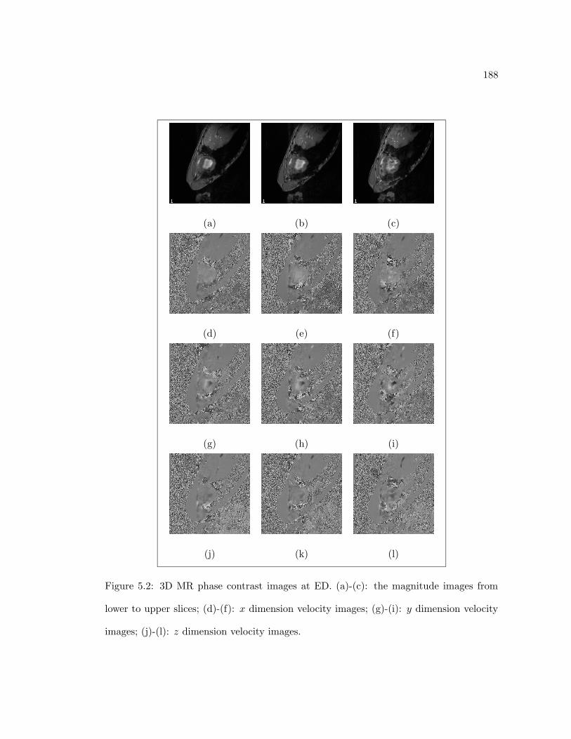
188

(a) (b) (c)

(d) (e) (f)

(g) (h) (i)

(j) (k) (l)

Figure 5.2: 3D MR phase contrast images at ED. (a)-(c): the magnitude images from

lower to upper slices; (d)-(f): x dimension velocity images; (g)-(i): y dimension velocity

images; (j)-(l): z dimension velocity images.

189

(a) (b)

(c) (d)

Figure 5.3: Myocardial Surfaces derived from phase contrast MR images. (a): the endo-

cardial potential energy map; (b): the endocardial surface wireframe; (c): the epicardial

potential energy map; (d): the endocardial surface wireframe.

three interpolated contours to every two consecutive data contours. Figure 5.3 shows the

potential energy maps and the wireframes of the interpolated endocardial and epicardial

surface at end diastole. The shape-based surface motion tracking process is then applied

to the sixteen interpolated surface sequences, once for the endocardium and once for the

epicardium. This way, the surface displacements have 1.09mm in-plane resolution and

1.25mm inter-plane resolution. A subset of the surface point displacements (ten percent)

is used as the boundary displacement constraint in the integrated volumetric framework.

The velocity images still have 5mm inter-plane resolution. To deal with this

problem, we have either inserted three tri-linearly interpolated velocity images into every

190

two data velocity images, or for computational reasons, we have coarsely re-sampled the

in-plane images to reduce the in-plane resolution to 4.36mm. In the example given in

this section, the velocity images are re-sampled to lower resolution to save computation

time. The mid-wall velocity of the phase contrast images is used as the initial velocity

constraint in the integrated volumetric framework.

In the case where the velocity images are re-sampled to lower resolution, the

myocardial surfaces are also re-sampled to the same lower resolutions of 4.36mm/pixel

in-plane and 5mm/pixel inter-plane after the surface motion tracking has been performed.

This way, even though the final re-sampled dataset has only 4.36mm in-plane and 5mm

inter-plane resolutions to form larger tetrahedral elements to save computational expense,

the boundary displacements still have 1.09mm in-plane and 1.25mm inter-plane resolu-

tions. The myocardial sample points which are bounded by the endocardial and epicardial

boundaries are Delaunay tessellated to form the finite element mesh of the myocardium.

Figure 5.4 shows the low resolution tetrahedral finite element mesh of the mid-ventricle

covered by the three-slice image set. In this case, there are 2147 tetrahedra in the mesh.

After the boundary displacement tracking process, the velocity image re-sampling

process, and the finite element mesh construction process, we can now perform the inte-

grated volumetric motion and deformation analysis. Following the procedures established

in the previous sections, the governing equations of the myocardium are derived from the

minimum potential energy principle. A linear isotropic elastic myocardial model is used,

and the material-related constants that have been established experimentally for the

myocardium in the biomechanics literature[138] are used, with Young’s modulus set to

be 75, 000Pascal, Poisson’s ratio set to around 0.5, the myocardial mass density set to

1.5gram/mm3, and the damping parameter set to under 0.1. The velocity values at the

191

Figure 5.4: Volumetric finite element mesh of the mid-ventricle from phase contrast MR

images.

mid-wall points are used as the initial velocity conditions, and the surface displacements

are used as the displacement boundary conditions. Since the temporal resolution of the

dataset is 0.03125sec/frame, we choose the integration time step ∆t = 0.003125sec to

have 10 integrated steps. Using these constraints and parameters, the motion and defor-

mation parameters of the myocardium at all sixteen time frames are calculated using the

Newmark integration process. In the experiment shown here, there are 2147 tetrahedra

in the finite element mesh. The required computer memory for the system to handle this

data set is around 60 MB. The computation time for each pair of images is about 10

hours on a Silicon Graphics Indigo2 workstation with 150 MHZ R4400 processor.

192

Figure 5.5: Dense field displacement vector map (2D projection) from the integrated

framework. Note the non-homogeneous nature of the myocardial motion.

Figure 5.5 presents the two-dimensional projection of the three-dimensional dense

field displacement vector map of the middle slice from ED to the next time frame, found

from the integrated framework. The use of 2D projections instead of a true 3D vector

map is only because of the ease of visualization. Here, a vector arrow begins from its

position at present time (ED), and ends at its position in the next time frame. The non-

homogeneous nature of the myocardial motion is very evident from this displacement

map: different regions of the myocardium display very different motion characteristics in

direction and magnitude.

While the displacements or path lengths of the myocardial points are useful for

193

predicting the state of health of the left ventricle, as discussed in Chapter 4, the element

strain tensors of the myocardial tissues provide the non-homogeneous deformation infor-

mation among regions which could be used to quantify transmural function, especially

issues related to the extent of myocardial injury[43]. Even though we believe more de-

tailed and sophisticated analysis on a range of image datasets under different physiological

conditions is required to infer any useful information for clinical and research purposes,

we still proceed to compute the strain measures on this particular dataset to test the ca-

pability of our integrated framework. To that end, we have calculated the strain tensors

for each tetrahedral element of the finite element grid to depict the non-rigid deforma-

tion, excluding the rigid bulk motion of the elements. Figure 5.6 shows the three normal

components (xx, yy, and zz components) and three shear components (xy, yz and zx

components) of the strain tensor for the deformation between ED and ES. It seems that

these three slices of mid-ventricle myocardium undergo very little z direction deformation.

The large strain at lower left part of the LV may be explained by the disconnected motion

caused by the infarction (we want to emphasize that this is a very intuitive explanation

for these strain maps, there should be no conclusion drawn from this initial experiment).

Figure 5.7 shows the more object-centered principal strain maps of the same deformation:

the three principal components of the strain as well as the two-dimensional projections

of the three-dimensional dense directions of the maximum principal strain (middle slice).

Once again, large strain is observed at the lower left part of the LV. In both Figure 5.6

and 5.7, the strain values are mapped back to the myocardial grid at its original state

(ED). In these figures, the negative strain values (contraction) are represent by different

shades of blue, and the positive values (expansion) are represent by different shades of

red.

194

(a) (b) (c)

(d) (e) (f)

−35% 0% 35% −20% 0% 2 0%

(g) (h)

Figure 5.6: 3D strain maps of mid-ventricle (ED-ES). (a): x-direction normal strain;

(b): y-direction normal strain; (c): z-direction normal strain; (d): xy-direction shear

strain; (e): yz-direction shear strain; (f): zx-direction shear strain; (g): color scale for

x-direction normal strain; (h): color scale for all other strains.

195

(a) (b)

(c) (d)

−35% 0% 35% −10% 0% 1 0%

(e) (f)

Figure 5.7: 3D principal strain maps of mid-ventricle (ED-ES). (a): the first (maximum)

principal strain; (b): the second principal strain; (c): the third (minimum) principal

strain; (d): two-dimensional projections of the three-dimensional directions of the max-

imum principal strain (middle slice). (e): color scale for the first and third principal

strains; (f): color scale for the second principal strains.

196

The temporal changes of the strain tensors are investigated and compared to ear-

lier observations available from biomechanics and cardiology literature [90, 132]. Since

we have only three mid-ventricle image slices, it is difficult to reliably define the radial,

longitudinal, and circumferential directions and the associated strain measures in those

directions which are commonly used in the cardiology community. Instead, the temporal

changes of the object-centered principal strains are compared to the data from literature.

Previously, the available principal strain data are often observed at isolated positions of

the myocardium varying from study to study. Here, we compare the average values of

strains of all the elements to these isolated strain data. In the literature[90, 132], the

values of the first (maximum) principal strain has been observed to reach a maximum

strain of 30% to 40% at ES, the second principal strain has very small values, and the

third (minimum) principal strain reaches an extreme value of −20% at ES. For our exper-

iment, we observe that the average value of the first principal strain reaches a maximum

strain of 32% at ES, the average second strain is very small and stable, and the third

principal strain reaches −18% at ES. Obviously, these results are very consistent with

previous studies. However, we should point out that our integrated motion and deforma-

tion framework can obtain dense motion and strain fields instead of only finding these

information at isolated positions, as was done previously. In addition, the framework’s

ability to quantify the difference of motion and deformation characteristics between my-

ocardial tissue elements makes it valuable to evaluate cardiac regional function. Figure

5.8 shows the temporal sequence of the first principal strain maps from ED to ES. Note

the different strain values between different regions.

We want to point out that although the integrated framework is intended to in-

tegrate complementary image constraints within a unified system, it also can be used

197

(a) (b) (c)

(d) (e) (f)

−40% 0% 4 0%

(g) (h) (i)

Figure 5.8: Temporal maps of the first principal strain (ED-ES) from phase contrast MR

images. (a)-(h): the eight principal strain maps from ED to ES; (i): color scale.

198

for motion and deformation analysis using only one image source. The uniqueness of

this framework is that it can take single or multiple image based data constraints, often

very noisy by themselves, and estimate the best compromise motion and deformation

parameters from these data and the mechanical model of the left ventricle, which pro-

vides a natural way to enforce the physically plausible potential energy functional and

smoothness constraints. Further, the actual physical constraints related to known cardiac

parameters such as pressure can also be incorporated into the system as external loads.

5.7 Conclusion

We have developed an integrated framework for the analysis of left ventricular motion and

deformation. This unified approach is based upon the use of image analysis strategies and

mechanical modelling of the myocardium, and is embedded in a finite element framework

for the integration of complementary image sources.

This integrated motion and deformation analysis framework estimates the op-

timal motion and deformation parameters from noisy and complementary image data.

Image-derived information from myocardial surfaces and the mid-wall are used in loca-

tions where they have the best signals. These data constraints are used as the initial and

boundary conditions in the system governing equations of the finite element framework.

A continuum mechanical model of the myocardium is applied to provide physically mean-

ingful constraints on the dynamic behaviors of the LV tissue. Stability and accuracy are

considered in seeking the solution to the system.

Experiments have been performed on one canine MR phase contrast image set.

Motion and deformation parameters are estimated from the integration of boundary dis-

placement information and mid-wall phase velocity information. Results have been com-

199

pared to previous studies in the literature.

Chapter 6

Summary

This thesis presents an integrated system for recovering motion and deformation of the

left ventricle from three-dimensional image sequences. The goal of this work is to combine

physical properties of the left ventricle with multiple, complementary sources of imaging

data to depict temporal motion and deformation parameters. The algorithms have been

implemented, and experiments have been conducted using real medical images of normal

and infarcted canine hearts with favorable results.

The geometrical representation of the left ventricle is obtained using the three-

dimensional constrained and bounded Delaunay tessellation of the myocardial sample

points. The endocardial and epicardial surfaces are characterized by the differential geo-

metrical properties of the multi-scale local surface patches, based on multi-order natural

neighbor relationships. The surface displacement field is estimated by matching points of

temporally consecutive surface frames based on geometrical similarity and a local smooth-

ness constraint. The accuracy of the surface point tracking has been validated by the

gold-standard of the implanted image-opaque physical markers. The MR phase images

provide robust instantaneous velocity at the mid-wall region. A finite element frame-

200

201

work is established by using the Delaunay tessellation of the left ventricle as the finite

element mesh. Continuum mechanical models of the myocardium are discussed, and a

linear isotropic elastic model is adopted in the framework. Using the minimum potential

energy principle, governing equations of system are established. The shape-based surface

displacements are used as the boundary conditions, and the phase velocity images are

used as the initial conditions in solving the governing equations. Displacement and strain

measures are derived from the solution of the system, and are compared to the results in

the literature.

We have exploited an attractive new research direction of using continuum me-

chanical models as a mean to guide dynamic information analysis from complementary

imaging data. The approach provides a natural framework to integrate physical informa-

tion of the object with visual image constraints. This model-based, integrated strategy

should allow us to obtain more robust descriptions of motion and deformation of the

myocardial wall.

There are, of course, several areas of potential improvement for this work. First

of all, this work only deals with frame-to-frame motion and deformation. There has been

no efforts in incorporating temporal motion and deformation models into the framework.

The periodic nature of the cardiac motion should provide a basis to enforce some temporal

constraints[61]. This work should also benefit from refining the motion and deformation

estimation by minimizing the errors between the position and velocity predictions of the

system equations and the image data position and velocity. We have done initial work

in this regard using a recursive feedback mechanism in the two-dimensional case (see

Appendix A). Extension to three-dimensions is needed.

Appendix A

2D Feedback Mechanism

When using the finite element framework to track motion between temporal images, it

can be regarded as a predictor from time t0 to time t1. Since we already have data

information at t1 in terms of the segmented endocardial and epicardial contours, as well

as the mid-wall velocities, we can refine the mapping estimate between frames t0 and t1

by comparing how close the image-driven, model-based prediction comes to the actual

data. The differences between the data and the prediction can be used as a recursive

feedback term to improve the matching process. Here, we report our progress in using

the boundary difference as the feedback force[115].

In the two-dimensional case, contour shape landmarks are defined as locally ex-

treme curvature points or curvature zero-crossing points. Making the curvature zero-

crossing points part of the landmark set ensures that any contour segment between two

consecutive landmarks will not change curvature sign if we traverse the segment from one

end to the other. In other words, all the contour segments constructed by the consecutive

landmarks will be either constant convex, or constant concave, or a straight line.

In the integration of displacement and velocity process, the boundary displace-

202

203

ment constraint is only enforced at the matching vectors which terminate at the landmark

points of the second contour. This way, the real and predicted contours at time t1 in-

tersect at these points. The contour segment defined by two consecutive landmarks of

the real data will always be either constant convex, or constant concave, or a straight

line. The corresponding predicted contour segment should be close to the real one in the

same classification sense, if the initial shape-based boundary matching is reasonably good

and the contour segment is not too large. In practice, these two requirements are readily

satisfied. In the feedback process, predicted contour segments are compared to actual

ones, based on a metric related to the similarity between pairs of actual and predicted

contour segments. To date, two curve comparison metrics have been developed, and have

shown similar effects in improving the matching process.

The first metric uses the shape matching idea that our initial boundary matching

is based upon. We were using point-wise shape comparison in the matching process, but

now we have to compare the entire curve segments. We define that the total tension for

any curve segment C equal to its normalized total curvature:

T (C) =∫

C|κ(s)| ds (A.1)

Since we have stated that the real and predicted contour segments would be close in

the sense of constant convexity or concavity, the total tension of any curve segment will

indicate its total curvedness. Furthermore, since the whole real contour can be treated

as if it were in an equilibrium state with respect to tension, the total tension difference

(termed as expanding force f(P)) between the corresponding predicted segment P and

the real segment R can be used as a target as to how much the predicted segment should

204

increase or decrease its tension:

f(P) = T (P)− T (R) (A.2)

A positive f(P) indicates that the segment has a tendency to expand along the out-

ward tangent directions of the two end points, while negative f(P) implies the shrinking

tendency. Since the neighboring segments interact at their common end point, the net

expanding force of the two segments determines the net expanding or shrinking tendency

of the common landmarks.

The second comparison metric simply defines the total tension for any given curve

segment equal to the normalized area of the segment (closed by the line connecting the

two end points). The expanding force is again defined as the total tension difference

between the corresponding predicted and real segments.

Figure A.1 illustrates the contour segment comparison idea described above. Here,

the solid line represents the real contour, and the dotted line is the predicted contour.

Segments A and C have an expanding tendency, while segment B is inclined to shrink.

However, the net force at the common end of A and B causes that landmark expand (or

shrink from B’s standpoint) into B, while the net force at the common end of B and C

is minimal (no change).

After forming the net expanding force at each landmark point, adjustments are

made for the initial boundary displacements. Displacement vectors emanating from the

first image frame are modified so they will end on the boundary of the second image, at

one side or another of the original matching landmarks, depending on the magnitude and

direction of the net expending force of each landmark. In Figure A.1, the common point

205

Segment C

f(A)

f(B)

f(B)f(C)

Segment A Segment B

Figure A.1: Compute the landmark net expanding-shrinking force in the feedback mech-

anism.

of segments A and B has net expanding force (it is positive), hence it should moves to

the right (expanding from segment A’s view and shrinking from segment B’s view). The

new displacement is then applied into the integrated finite element framework to compute

refined motion information.

Figure A.2 illustrates the effect of the feedback mechanism. (a) is the original

grid, (d) is the target data grid at the next time frame. (b) is the system predicted grid

without any corrections, while (c) is the refined prediction after two steps of feedback

correction at the boundaries. We can see the local and overall improvement of the refined

prediction.

206

(a) (b)

(c) (d)

Figure A.2: Effect of the feedback mechanism. (a): original grid; (b): predicted grid

without feedback; (c): predicted grid with two feedback iterations; (d): actual data grid.

Bibliography

[1] A. Amini, P. Anandan, and J. S. Duncan. Non-rigid motion models for tracking the

left ventricular wall. In Information Processing in Medical Imaging, Kent, England,

July 1991.

[2] A. Amini, R. Curwen, and J. Gore. Snakes and splines for tracking non-rigid heart

motion. In European Conference on Computer Vision, Cambridge, England, 1996.

[3] A. A. Amini and J. S. Duncan. Bending and stretching models for LV wall motion

analysis from curves and surfaces. Image and Vision Computing, 10(6):418–430,

1992.

[4] A. A. Amini and J. S. Duncan. Differential geometry for characterizing 3D shape

change. SPIE- Mathematical Methods in Medical Imaging, 1768:170–181, 1992.

[5] P. Anandan. A computational framework and an algorithm for the measurement

of visual motion. International Journal of Computer Vision, 2:283–310, 1989.

[6] J. Areeda, E. Garcia, K. Vantrain, D. Brown, A.Waxman, and D. Berman. A

comprehensive method for automatic analysis of rest/exercise ventricular function

from radionuclide angiography. In Digital Imaging: Clinical Advances in Nuclear

Medicine, pages 241–256. Society of Nuclear Medicine, 1982.

207

208

[7] T. Arts, R. S. Reneman, et al. Measurement of deformation of canine epicardium in

vivo during cardiac cycle. American Journal of Physiology, 239:H432–H437, 1980.

[8] L. Axel and L. Dougherty. MR imaging of motion with spatial modulation of

magnetization. Radiology, 171:841–845, 1989.

[9] Azhari et al. Noninvasive quantification of principal strains in normal canine hearts

using tagged MRI images in 3D. American Journal of Physiology, 264:H205–H216,

1993.

[10] H. Baker. Surface reconstruction from image sequences. In Proceedings of the 2nd

International Conference on Computer Vision, pages 334–343, Tampa, December

1988.

[11] S. T. Barnard and W. B. Thompson. Disparity analysis of images. IEEE Transac-

tions on Pattern Analysis and Machine Intelligence, 2(4):333–340, 1980.

[12] K. Bathe and E. Wilson. Numerical Methods in Finite Element Analysis. Prentice-

Hall, New Jersey, 1976.

[13] Paul J. Besl and Ramesh C. Jain. Invariant surface characteristics for 3D object

recognition in range images. Computer Vision, Graphics and Image Processing,

33:33–80, 1986.

[14] R. Beyar et al. Quantification and validation of LV wall thickening by a 3D volume

element MRI approach. Circulation, 81:297–307, 1990.

[15] M. J. Black and Y. Yacoob. Tracking and recognizing rigid and non-rigid facial

motions using local parametric models of image motion. In Fifth International

Conference on Computer Vision, pages 374–381, 1995.

209

[16] J. D. Boissonnat. Shape reconstruction from planar cross-sections. Computer Vi-

sion, Graphics, Image Processing, 44:1–29, 1988.

[17] E. L. Bolson, S. Kliman, F. Sheehan, and H. T. Dodge. Left ventricular segmental

wall motion - A new method using local direction information. In Proceedings of

Computers in Cardiology, 1980.

[18] F. L. Bookstein. Principal warps: Thin-plate splines and the decomposition of

deformations. IEEE Transactions on Pattern Analysis and Machine Intelligence,

pages 567–585, 1989.

[19] G. Borgefors. Distance transformations in arbitrary dimensions. Computer Vision,

Graphics and Image Processing, 27:321–345, 1984.

[20] G. Borgefors. Distance transformations in digital images. Computer Vision, Graph-

ics and Image Processing, 34:344–371, 1986.

[21] A. Chakraborty, L. H. Staib, and J. S. Duncan. An integrated approach to boundary

finding in medical images. In Proceedings of the IEEE Workshop on Biomedical

Image Analysis, pages 13–22, 1994.

[22] J. Chesebro, G. Knatterrud, and others. Thrombolysis in myocardial infarction

(TIMI) trial phase I: A comparison between intravenous tissue plasminogen activa-

tor and intravenous streptokinase. Circulation, 76:142–154, 1987.

[23] P. Clayton, G. Jepson, and S. Klausner. Should a fixed external reference system be

used to analyze left ventricular wall motion? Circulation, 65(7):1518–1521, 1982.

210

[24] R.T. Constable, K. Rath, A. Sinusas, and J. Gore. Development and evaluation

of tracking algorithms for cardiac wall motion analysis using phase velocity MR

imaging. Magnetic Resonance in Medicine, 32:33–42, 1994.

[25] R. Courant and D. Hilbert. Methods of Mathematical Physics. Interscience, London,

1957.

[26] L. L. Creswell, M. J. Moulton, S. G. Wyers, J. S. Pirolo, D. S. Fishman, W. H.

Perman, K. W. Myers, R. L. Actis, M. W. Vannier, B. A. Szabo, and M. K. Pasque.

An experimental method for evaluating constitutive models of myocardium in in

vivo hearts. American Journal of Physiology, 267:H853–H863, 1994.

[27] M. Dae, J. Herre, and et al. Scintigraphic assessment of sympathetic innervation

after transmural versus nontransmural myocardial infarction. Journal of American

College of Cardiology, 17:1416–1423, 1991.

[28] T. Denney and J. L. Prince. 3D displacement field reconstruction from planar

tagged cardiac MR images. In Proceedings of the IEEE Workshop on Biomedical

Image Analysis, pages 51–60, 1994.

[29] M. P. do Carmo. Differential Geometry of Curves and Surfaces. Prentice-Hall, New

Jersey, 1976.

[30] A. S. Douglas, W. C. Hunter, and M. D. Wiseman. Inhomegeneous deformation

as a source of error in strain measurements derived from implanted markers in the

canine left ventricle. Journal of Biomechanics, 23:331–341, 1990.

211

[31] L. Eaton and B. Bulkley. Expansion of the acute myocardial infarction: its rela-

tionship to infarct morphology in a canine model. Circulation Research, 49:80–88,

1981.

[32] I. A. Essa and A. P. Pentland. Facial expression recognition using a dynamic model

and motion energy. In Fifth International Conference on Computer Vision, pages

360–367, 1995.

[33] T. Faber, E. Stokely, G. Templeton, et al. Quantification of three-dimensional left

ventricular segmental wall motion and volumes from gated tomographic radionu-

clide ventriculograms. Journal of Nuclear Medicine, 30:638–649, 1989.

[34] O. Faugeras. Three-dimensional Computer Vision: A Geometric Viewpoint. MIT

Press, 1993.

[35] C. A. Felippa and R. W. Clough. The finite element method in solid mechanics. In

SIAM-AMS Proceedings, volume 2, pages 210–252, Providence, RI, 1970.

[36] J. D. Foley, A. van Dam, S. K. Feiner, and J. F. Hughes. Computer Graphics:

Principles and Practice. Addison-Wesley, 1990.

[37] H. Fuchs, Z. M. Kedem, and S. P. Uselton. Optimal surface reconstruction from

planar contours. Communications of ACM, 20:693–702, 1977.

[38] Y. C. Fung. A First Course in Continuum Mechanics. Prentice-Hall, 1977.

[39] H. Gelberg, B. Brundage, S. Glantz, and W. Parmley. Quantitative left ventricular

wall motion analysis: A comparison of area, chord and radial methods. Circulation,

59(5):991–1000, 1979.

212

[40] D. Gibson, T. Prewitt, and D. Brown. Analysis of left ventricular wall movement

during isovolumic relaxation and its relation to coronary artery disease. British

Heart Journal, 38:1010, 1976.

[41] F. Glazer, G. Reynolds, and P. Anandan. Scene matching by hierarchical corre-

lation. In Proceedings of the IEEE Conference on Computer Vision and Pattern

Recognition, pages 432–441, 1983.

[42] L. Goncalves, E. Di Bernardo, E. Ursella, and P. Perona. Monocular tracking of the

human arm in 3D. In Fifth International Conference on Computer Vision, pages

764–770, 1995.

[43] W. Grossman. Assessment of regional myocardial function. Journal of American

College of Cardiology, 7(2):327–328, 1986.

[44] J. M. Guccione, A. D. McCulloch, and L. K. Waldman. Passive material properties

of intact ventricular myocardium determined from a cylindrical model. Journal of

Biomechanical Engineering, 113:42–55, 1991.

[45] K. Gupta, M. Ratcliffe, M. Fallert, L. Edmunds, and D. Bogen. Changes in passive

mechanical stiffness of myocardial tissue with aneurysm formation. Circulation,

89:2315–2326, 1994.

[46] M. Guttman, J. L. Prince, and E. R. McVeigh. Contour estimation in tagged

magnetic resonance images. IEEE Transactions on Medical Imaging, 13:74–88,

1994.

213

[47] L. Harris, P. Clayton, H. Marshall, and H. Warner. A technique for the detection

of asynergistic motion in the left ventricle. Computers and Biomedical Research,

7:380–394, 1974.

[48] R. J. Herfkens, N. J. Pelc, L. R. Pelc, and J. Sayre. Right ventricular strain

measured by phase contrast MRI. In Proceedings of the 10th Annual Society of

Magnetic Resonance Medicine, page 163, San Francisco, 1991.

[49] G. T. Herman, J. Zheng, and C. A. Bucholtz. Shape-based interpolation. IEEE

Computer Graphics and Applications, pages 69–79, 1992.

[50] E. C. Hildreth. The Measurement of Visual Motion. MIT Press, Cambridge, 1984.

[51] H. Honda, Y. Koiwa, K. Takagi, J. Kikuchi, N. Hoshi, T. Takishima, and J. P.

Butler. Noninvasive measurement of left ventricular myocardial elasticity. American

Journal of Physiology, pages H881–H890, 1994.

[52] B. K. P. Horn. Robot Vision. MIT Press, Cambridge, 1986.

[53] B. K. P. Horn and B. G. Schunck. Determining optical flow. Artificial Intelligence,

17:185–203, 1981.

[54] B. Horowitz and S. Pentland. Recovery of non- rigid motion and structure. In

Proceedings of the IEEE Conference on Computer Vision and Pattern Recognition,

pages 325–330, Maui, June 1991.

[55] W. C. Huang and D. B. Goldgof. Adaptive-size physically-based models for nonrigid

motion analysis. In Proceedings of the IEEE Conference on Computer Vision and

Pattern Recognition, pages 833–835, 1992.

214

[56] K. H. Huebner, E. A. Thornton, and T. G. Byrom. The Finite Element Method

For Engineers. John Wiley & Sons, New York, 1995.

[57] J. D. Humphrey and F. C. P. Yin. Biomechanical experiments on excised my-

ocardium: theoretical considerations. Journal of Biomechanics, 22:377–383, 1990.

[58] P. J. Hunter, A. McCulloch, P. Nielsen, and B. Smaill. A finite element model

of passive ventricular mechanics. Computational Methods in Bioengineering, pages

387–397, 1988.

[59] P. J. Hunter, P. M. F. Nielsen, B. H. Smaill, and I. J. LeGrice. An anatomical

heart model with applications to myocardial activation and ventricular mechanics.

Critical Reviews in Biomedical Engineering, 20:403–426, 1992.

[60] P. J. Hunter and B. H. Smaill. The analysis of cardiac function: a continuum

approach. Progress in Biophysics and Molecular Biology, 52:101–164, 1989.

[61] J. C. McEachen II, A. Nehorai, and J. S. Duncan. A recursive filter for temporal

analysis of cardiac motion. In Proceedings of the IEEE Workshop on Biomedical

Image Analysis, pages 124–133, 1994.

[62] M. Iri, T. Koshizuka, and T. Ohya. A fast Voronoi-diagram with applications to

geographical optimization problem. In Lecture Notes in Control and Information

Science: System modelling and Optimization, pages 273–288, 1984.

[63] C. Kambhamettu and D. Goldgof. Point correspondence recovery in non–rigid

motion. In Computer Vision and Pattern Recognition, pages 222–227, June 1992.

[64] M. Kass, A. Witkin, and D. Terzopoulos. Snakes: Active contour models. Interna-

tional Journal of Computer Vision, pages 321–331, 1989.

215

[65] E. Keppel. Approximating complex surfaces by triangulation of contour lines. IBM

Journal of Research and Development, 19:2–11, 1975.

[66] D. King, A. Gopal, A. Keller, et al. Three- dimensional echocardiography: Advances

for measurement of volume and mass. Hypertension, 23(suppl. I):I172–I179, 1994.

[67] J. J. Koenderink and A. J. van Doorn. Surface shape and curvature scale. Image

and Vision Computing, 10(8):557–565, 1992.

[68] J. Links, K. Douglass, and H. Wagner. Patterns of ventricular emptying by fourier

analysis of gated blood pool studies. Journal of Nuclear Medicine, 21:978–982,

1980.

[69] G. E. Mailloux, A. Bleau, M. Bertrand, and R. Petitclerc. Computer analysis

of heart motion from two dimensional echocardiograms. IEEE Transactions on

Biomedical Engineering, BME-34(5):356–364, May 1987.

[70] D. Marr. Vision. W. H. Freeman and Co., 1982.

[71] A. McCulloch, L. Waldman, J. Rogers, and J. Guccione. Large-scale finite element

analysis of the beating heart. Critical Reviews in Biomedical Engineering, 20:427–

449, 1992.

[72] A. D. McCulloch and J. H. Omens. Non–homogeneous analysis of three–dimensional

transmural finite deformation in canine ventricular myocardium. J. Biomechanics,

24:539–548, 1991.

[73] D. McPherson, D. Skorton, et al. Finite element analysis of myocardial diastolic

function using three-dimensional echocardiographic reconstructions: application of

216

a new method for study of acute ischemia in dogs. Circulation Research, 60:674–682,

1987.

[74] D. Metaxas and D. Terzopoulos. Constrained deformable superquadrics and non-

rigid motion tracking. In Proceedings of the IEEE Conference on Computer Vision

and Pattern Recognition, pages 337–343, 1991.

[75] F. G. Meyer, R. T. Constable, A. G. Sinusas, and J. S. Duncan. Tracking myocardial

deformation using spatially constrained velocities. In Information Processing in

Medical Imaging. Kluwer, 1995.

[76] D. Meyers and S. Skinner. Surfaces from contours. ACM Transactions on Graphics,

11:228–258, July 1992.

[77] S. Mishra, D. Goldgof, and T. Huang. Motion analysis and epicardial deforma-

tion estimation from angiography data. In Proceedings of the IEEE Conference on

Computer Vision and Pattern Recognition, pages 331–336, Maui, June 1991.

[78] C. Moore, W. O’Dell, E. McVeigh, and E. Zerhouni. Calculation of three-

dimensional left ventricular strains from biplanar tagged MR images. Journal of

Magnetic Resonance Imaging, 2:165–175, 1992.

[79] H. H. Nagel and W. Enkelmann. An investigation of smoothness constraints for the

estimation of displacement vector fields from image sequences. IEEE Transactions

on Pattern Analysis and Machine Intelligence, 8:565–593, 1986.

[80] C. Nastar and N. Ayache. Non-rigid motion analysis in medical images: a physically

based approach. In Information Processing in Medical Imaging. Springer-Verlag,

1993.

217

[81] G. Nayler, N. Firmin, and D. Longmore. Blood flow imaging by cine magnetic

resonance. Journal of Computer Assisted Tomography, 10:715–722, 1986.

[82] N. M. Newmark. A method of computation for structure dynamics. Journal of

Enginering Mechanics Division, 85:67–94, 1959.

[83] S. A. Niyogi and E. H. Adelson. Analyzing gait with spatiotemporal surfaces. In

Proceedings of the workshop on motion of non-rigid and articulated bodies, pages

16–24, November 1994.

[84] V. P. Novak, F. C. P. Yin, and J. D. Humphrey. Regional mechanical properties of

passive myocardium. Journal of Biomechanics, 27(4):403–412, 1994.

[85] W.G. O’Dell, C.C. Moore, W. Hunter, E.A. Zerhouni, and E.R. McVeigh. Dis-

placement field fitting for calculating 3D myocardial deformations from tagged MR

images. Radiology, 195:829–835, 1995.

[86] M. O’Donnell, A. Skovoroda, B. Shapo, and S. Emelianov. Internal displacement

and strain imaging using ultrasonic speckle tracking. IEEE Transactions on Ultra-

sonic Ferroelectrics and Frequency Control, 41:314–325, 1994.

[87] T. Ohya, M. Iri, and K. Murota. Improvements of the incremental method for

Voronoi diagram with computational comparisons of various algorithms. Journal

of the Operation Research Society of Japan, 27:306–336, 1984.

[88] A. Okabe, B. Boots, and K. Sugihara. Spatial Tessellations: Concepts and Appli-

cations of Voronoi Diagrams. John Wiley & Sons, 1992.

[89] E. R. A. Oliveira. Theoretical foundations of the finite element method. Interna-

tional Journal Solid Structure, 4:929–952, 1968.

218

[90] J. H. Omens, D. A. MacKenna, and A. D. McCulloch. Measurement of strain and

analysis of stress in resting rat left ventricular myocardium. Journal of Biomechan-

ics, 26(6):665–676, 1993.

[91] J. O’Rourke. Computational Geometry in C. Cambridge University Press, 1993.

[92] R. Owen, L. Staib, P. Anandan, and J. Duncan. Measurement of non-rigid motion

in images using contour shape descriptors. In Proceedings of the IEEE Conference

on Computer Vision and Pattern Recognition, 1991.

[93] K. Palaniappa, C. Kambhamettu, A. F. Hasler, and D. B. Goldgof. Structure and

semi-fluid motion analysis of stereoscopic satellite images for cloud tracking. In

Fifth International Conference on Computer Vision, pages 659–665, 1995.

[94] J. Park, D. Metaxas, and L. Axel. Volumetric deformable models with parameter

functions: a new approach to the 3D motion analysis of the LV from MRI-SPAMM.

In Fifth International Conference on Computer Vision, pages 700–705, 1995.

[95] J. Park, D. Metaxas, and A. Young. Deformable models with parameter functions:

application to heart-wall modeling. In Proceedings of the IEEE Conference on

Computer Vision and Pattern Recognition, pages 437–442, 1994.

[96] N. J. Pelc and M. A. Bernstein. Optimized encoding for phase contrast flow

measurement. In Proceedings of the 9th Annual Society of Magnatic Resonance

Medicine, page 475, New York, 1990.

[97] N. J. Pelc, R. J. Herfkens, and L. R. Pelc. 3D analysis of myocardial motion

and deformation with phase contrast cine MRI. In Proceedings of the 11th Annual

Society of Magnatic Resonance Medicine, page 18, Berlin, 1992.

219

[98] N. J. Pelc, R. J. Herfkens, A. Shimakawa, and D. Enzmann. Phase contrast cine

magnetic resonance imaging. Magnetic Resonance Quarterly, 7(4):229–254, 1991.

[99] N. J. Pelc, A. Shimakawa, and G. H. Glover. Phase contrast cine MRI. In Pro-

ceedings of the 8th Annual Society of Magnatic Resonance Medicine, page 101,

Amsterdam, 1989.

[100] C. Peskin and D. McQueen. Cardiac fluid dynamics. In T. Pilington, editor, High

Performance Computing in Biomedical research, pages 51–59. CRC Press, 1993.

[101] M. Pfeffer and E. Braunwald. Ventricular remodeling after myocardial infarction:

experimental observations and clinical implications. Circulation, 81:1161–1172,

1990.

[102] K. Raghavan and A. Yagle. Forward and inverse problems in imaging the elasticity

of soft tissue. IEEE Transactions on Nuclear Science, 41(4):1639–1647, 1994.

[103] V. T. Rajan. Optimality of the delaunay triangulation in Rd. Discrete and Com-

putation Geometry, 12:189–202, 1994.

[104] E. L. Ritman. State of the art and future perspectives-fast CT for quantitative

cardiac analysis. Mayo Clinic Proceedings, 65:1336–1349, 1990.

[105] E. L. Ritman, J. H. Kinsey, L. D. Harris, and R. A. Robb. Some imaging require-

ments for quantification of structure and function of the heart. In M. D. Short, D. A.

Pay, S. Leeman, and R. M. Harrison, editors, Physical Techniques in Cardiological

Imaging, pages 189–198. Adam Hilger, Ltd., 1982.

[106] R. A. Robb. High-speed three-dimensional x-ray computed tomography: The dy-

namic spatial reconstructor. Proceedings of the IEEE, 71:308–319, 1983.

220

[107] Azriel Rosenfeld and Avinash C. Kak. Digital Picture Processing. Academic Press,

1st edition, 1976.

[108] M. Sambridge, J. Braun, and H. McQueen. Geophysical parameterization and

interpolation of irregular data using natural neighbours. Geophysical Journal In-

ternational, 122:837–857, 1995.

[109] P. T. Sander and S. W. Zucker. Inferring surface trace and differential structure

from 3D images. IEEE Transactions on Pattern Analysis and Machine Intelligence,

12(9):833–854, 1990.

[110] S. Sclaroff and A. P. Pentland. Modal matching for correspondence and recognition.

IEEE Transactions on Pattern Analysis and Machine Intelligence, 17(6):545–561,

1995.

[111] M. I. Shamos. Computational Geometry. PhD thesis, Yale University, New Haven,

CT, 1978.

[112] F. H. Sheehan, E. L. Bolson, H. T. Dodge, and others. Advantages and appli-

cations of the centerline method for characterizing regional ventricular function.

Circulation, 74:293–305, 1986.

[113] P. Shi, A. Amini, R.T. Constable, and J. Duncan. Tracking tagged MR images with

energy-minimizing deformable grids. In Proceedings of 18th IEEE Annual Northeast

Bioengineering Conference, pages 133–134, 1992.

[114] P. Shi, A. Amini, G. Robinson, A. Sinusas, R. T. Constable, and J. Duncan. Shape-

based 4D left ventricular myocardial function analysis. In Proceedings of the IEEE

Workshop on Biomedical Image Analysis, pages 88–97, 1994.

221

[115] P. Shi, G. Robinson, R. T. Constable, A. Sinusas, and J. Duncan. A model-based

integrated approach to track myocardial deformation using displacement and ve-

locity constraints. In Fifth International Conference on Computer Vision, pages

687–692, 1995.

[116] P. Shi, G. Robinson, and J. Duncan. Myocardial motion and function assessment

using 4D images. In Visualization in Biomedical Computing, pages 148–159, 1994.

[117] R. Sibson. A brief description of natural neighbor interpolation. In Interpreting

Multivariate Data, New York, 1981. John Wiley.

[118] A. J. Sinusas, K. A. Trautman, J. D. Bergin, D. D. Watson, M. Ruiz, W. H. Smith,

and G. A. Beller. Quantification of area at risk during coronary occlusion and de-

gree of myocardial salvage after reperfusion with technetium-99m methoxyisobutyl

isonitrile. Circulation, 82:1424–1437, 1990.

[119] S. Siu, M. Rivera, and et al. Three- dimensional echocardiography: In vivo vali-

dation for left ventricular volume and function. Circulation, 88(part 1):1715–1723,

1993.

[120] C. Slager, T. Hooghoudt, P. Serruys, J. Schuurbiers, and J. Reiber et al. Quanti-

tative assessment of regional left ventricular motion using endocardial landmarks.

Journal of American College of Cardiology, 7(2):317–326, 1986.

[121] B. H. Smaill and P. J. Hunter. Structure and function of the diastolic heart: material

properties of the passive myocardium. In Theory of the heart, Berlin, 1991. Springer-

Verlag.

222

[122] S. Song and R. Leahy. Computation of 3D velocity fields from 3D cine CT images.

IEEE Transactions on Medical Imaging, 10:295–306, Sept 1991.

[123] A. Spencer. Continuum Mechanics. Longman, London, 1980.

[124] L. Staib and J. S. Duncan. Parametrically deformable contour models. IEEE Trans-

actions on Pattern Analysis and Machine Intelligence, 14(11):1061–1075, 1992.

[125] G. Taubin. Curve and surface smoothing without shrinkage. In Proceedings of the

Fifth International Conference on Computer Vision, pages 852–857, 1995.

[126] D. Terzopoulos and D. Metaxas. Dynamic 3D models with local and global defor-

mation: Deformable superquadrics. IEEE Transactions on Pattern Analysis and

Machine Intelligence, 13(17), 1991.

[127] D. Terzopoulos and M. Vasilescu. Sampling and reconstruction with adaptive

meshes. In Proceedings of the IEEE Conference on Computer Vision and Pattern

Recognition, pages 70–75, 1991.

[128] M. Tistarelli and G. Marcenaro. Using optical flow to analyze the motion of human

body organs from bioimages. In Proceedings of the IEEE Workshop on Biomedical

Image Analysis, pages 100–109, 1994.

[129] J. Udupa and G. Herman. 3D Imaging in Medicine. CRC Press, Boca Raton, 1991.

[130] S. Ullman. The Interpretation of Visual Motion. MIT Press, Cambridge, 1979.

[131] F. J. Villarreal, L. K. Waldman, and W. Y. W. Lew. A technique for measuring

regional two-dimensional finite strains in canine left ventricle. Circulation Research,

62:711–721, 1988.

223

[132] L. K. Waldman, Y. C. Fung, and J. W. Covell. Transmural myocardial deforma-

tion in the canine left ventricle: normal in vivo three–dimensional finite strains.

Circulation Research, 57:152–163, 1985.

[133] K. Washizu. Variational Methods in Elasticity and Plasticity. Pergamon, Elmsford,

NY, 1982.

[134] D. F. Watson. Computing the n-dimensional delaunay tessellation with application

to Voronoi polytopes. The Computer Journal, 24:167–172, 1981.

[135] D. F. Watson. Natural neighbor sorting on the n-dimensional sphere. Pattern

Recognition, 21:63–67, 1988.

[136] D. F. Watson and G. M. Philip. Neighborhood-based interpolation. Geobyte, 2:12–

16, 1987.

[137] V. Wedeen. Magnetic resonance imaging of myocardial kinematics: technique to

detect, localize and quantify the strain rates of active human myocardium. Magnetic

Resonance Medicine, 27:52–67, 1992.

[138] H. Yamada. Strength of Biological Material. The Williams and Wilkins Company,

Baltimore, 1970.

[139] A. A. Young and L. Axel. Three-dimensional motion and deformation in the heart

wall: estimation from spatial modulation of magnetization – a model-based ap-

proach. Radiology, 185:241–247, 1992.

[140] A. A. Young, L. Axel, L. Dougherty, D. Bogen, and C. Parenteau. Validation of

MRI tagging to estimate material deformation. Radiology, 188:101–108, 1993.

224

[141] A. A. Young, D. L. Kraitchman, and L. Axel. Deformable models for tagged MR

images: Reconstruction of two- and three-dimensional heart wall motion. In Pro-

ceedings of the IEEE Workshop on Biomedical Image Analysis, pages 317–323, 1994.

[142] I. T. Young, J. E. Walker, and J. E. Bowie. An analysis technique for biological

shape. I. Information and Control, 25(10):357–370, 1974.

[143] E. Zerhouni et al. Tagging of the human heart by multiplanar selective RF satura-

tion for the analysis of myocardial contraction. In Abstracts of the Annual Meeting

of the Society of Magnetic Resonance in Imaging, page 10, San Francisco, 1988.

[144] D. Zisserman et al. Cardiac catheterization and angiographic analysis computer

applications. Progress in Cardiovascular Diseases, XXV:409–434, 1983.