ABSTRACT

Title of Document: ROLE OF ON-BOARD SENSORS IN

REMAINING LIFE PROGNOSTIC

ALGORITHM DEVELOPMENT FOR

SELECTED ASSEMBLIES AS INPUT TO A

HEALTH AND USAGE MONITORING

SYSTEM FOR MILITARY GROUND

VEHICLES

Richard Heine, Ph.D., 2008

Directed By: Professor Donald Barker, Department of

Mechanical Engineering

Improved reliability of military ground vehicle systems is often in direct

conflict with increased functionality and performance. Health and Usage Monitoring

Systems or HUMS are being developed to address this issue. HUMS can be

practically defined as a system of sensors, processors and algorithms that give an

indication of remaining component life. Fatigue of metal components is a common

failure mode on military vehicles, and failures of this type have a major effect on

vehicle reliability and availability. The purpose of this research is to develop the

methods and algorithms necessary for applying HUMS and remaining life prognostics

to metal fatigue on a military wheeled vehicle.

A range of models were developed and fidelity of the models was shown to be

correlated with computational complexity. Simplistic models based on feature

recognition had the least potential for accurate fatigue damage predictions while high

fidelity physics-based models had the most potential. Recommendations for the

information needed to select the most appropriate model for a component and

optimize the effect on vehicle reliability and availability were discussed. Methods for

identifying the set of instrumentation that could reasonably be used as part of a

HUMS and techniques for selecting the instrumentation that provides inputs for metal

fatigue damage models were evaluated. Techniques for identifying critical data and

instrumentation were also described. The methods and algorithms developed were

demonstrated for a variety of components on a military wheeled vehicle, and

validation was performed by comparing the results of the remaining life prognostics

with those from high fidelity physics of failure models.

The processes developed could be easily adapted to other platforms including

commercial fleets of vehicles or aircraft. These algorithms and techniques provide

potential for improving reliability and availability, but it should be noted that other

methods may be more appropriate depending on the specific vehicle and failure

mode. Significant work remains to implement HUMS technologies on a military

wheeled vehicle, but increasing reliability and availability is a worthy goal.

ROLE OF ON-BOARD SENSORS IN REMAINING LIFE PROGNOSTIC

ALGORITHM DEVELOPMENT FOR SELECTED ASSEMBLIES AS INPUT TO

A HEALTH AND USAGE MONITORING SYSTEM FOR MILITARY GROUND

VEHICLES

By

Richard Heine

Dissertation submitted to the Faculty of the Graduate School of the

University of Maryland, College Park, in partial fulfillment

of the requirements for the degree of

Doctor of Philosophy

2008

Advisory Committee:

Professor Donald Barker, Chair

Professor Abhijit Dasgupta

Associate Professor Patrick McCluskey

Associate Professor Charles Schwartz

Adjunct Associate Professor Gregory Schultz

ii

Acknowledgements

I would like to take this opportunity to thank all of those who provided

support, motivation and assistance with this goal of completing doctoral dissertation

research. Thanks to my committee members and especially Professor Don Barker for

giving me the opportunity and support necessary to investigate an interesting topic of

value to the academic and military communities. Thanks to Drs. David Mortin, Tom

Stadterman and Mike Cushing for their inspiration, guidance, and patience. To

George and Yussef, many thanks for proof-reading and providing such insightful

comment to the seemingly endless supply of abstracts, papers and chapters. To my

colleagues at AMSAA, Greg, Nick, Lane, Matt, Dave, Jeff, Mike and John, thanks for

all the hard work in making this great distraction so transparent to our customers.

And finally, a special note of gratitude to my family and friends for their love,

support, and willingness to learn so much about this research.

iii

Table of Contents

Acknowledgements....................................................................................................... ii

Table of Contents......................................................................................................... iii

List of Tables ................................................................................................................ v

List of Figures .............................................................................................................. vi

Chapter 1: Introduction ................................................................................................. 1

1.1 Problem Statement ........................................................................................ 1

1.2 Background and Motivation ......................................................................... 2

1.3 Approach....................................................................................................... 5

1.4 Overview of Thesis ....................................................................................... 6

Chapter 2: HUMS Technology ..................................................................................... 8

2.1 Current HUMS Applications ........................................................................ 8

2.2 HUMS Functions ........................................................................................ 11

2.3 Implementation of HUMS in a Military Vehicle Life Cycle...................... 19

2.4 Summary..................................................................................................... 23

Chapter 3: Terrain Identification for Electronics........................................................ 25

3.1 Background ................................................................................................. 25

3.2 Demonstration Vehicle and Example Component...................................... 28

3.3 Terrain Identification .................................................................................. 29

3.3.1 Sample Statistics ................................................................................. 30

3.3.2 Evaluation Procedure .......................................................................... 33

3.3.3 Sample Window Size.......................................................................... 35

3.4 Fatigue Estimation ...................................................................................... 36

3.5 Results......................................................................................................... 37

3.6 Conclusions................................................................................................. 39

Chapter 4: Terrain Identification for Mechanical Components.................................. 41

4.1 Background ................................................................................................. 41

4.2 Demonstration Vehicle and Example Component...................................... 44

4.3 Terrain Identification .................................................................................. 46

4.3.1 Sample Statistics ................................................................................. 47

4.3.2 Evaluation Procedure .......................................................................... 49

4.3.3 Sample Window Size.......................................................................... 51

4.4 Fatigue Estimation ...................................................................................... 52

4.5 Results......................................................................................................... 53

4.6 Conclusions................................................................................................. 55

Chapter 5: Acceleration-Based Strain Estimation ...................................................... 57

5.1 Background ................................................................................................. 57

5.2 Demonstration Vehicle and Component..................................................... 62

5.3 Waveform Comparison............................................................................... 63

5.4 Fatigue Estimates ........................................................................................ 65

5.4.1 Maximum Excursion Scaling.............................................................. 66

5.4.2 Fatigue Damage Based Scaling .......................................................... 68

5.4.3 Potential Improvements ...................................................................... 70

5.5 Results......................................................................................................... 71

iv

5.6 Conclusions................................................................................................. 73

Chapter 6: Identifying Damage Indicators and Physics-Based Strain Estimation..... 74

6.1 Background ................................................................................................. 74

6.2 Demonstration Vehicle and Component..................................................... 79

6.3 Direct Strain Model..................................................................................... 80

6.3.1 Normalized Cross-Correlation ............................................................ 81

6.3.2 Coefficient of Determination of Root Mean Square........................... 84

6.4 Physics-Based Estimation........................................................................... 87

6.5 Hybrid Models ............................................................................................ 88

6.6 Results......................................................................................................... 90

6.7 Conclusions................................................................................................. 92

Chapter 7: Discussions and Summary ....................................................................... 95

7.1 Model Fidelity............................................................................................. 96

7.2 Instrumentation and Sensors ....................................................................... 99

7.2.1 Potential Sensors............................................................................... 100

7.2.2 Strain Indicators ................................................................................ 102

7.3 Summary and Contributions ..................................................................... 103

7.4 Limitations and Future Work.................................................................... 104

Appendix A............................................................................................................... 108

Appendix B ............................................................................................................... 109

Bibliography ............................................................................................................. 116

v

List of Tables

Table 3.1: Average fatigue damage per 20 seconds exposure .................................... 30

Table 4.1: Average fatigue damage per 20 seconds exposure .................................... 47

Table 5.1: Maximum excursion scaling...................................................................... 67

Table 5.2: Fatigue life scaling..................................................................................... 69

Table 6.1: Average normalized cross-correlation with strain..................................... 83

Table 6.2: Coefficient of determination of RMS with RMS strain............................. 86

Table 6.3: Physics-based comparison ......................................................................... 89

Table 6.4: 20,000 mile endurance test damage........................................................... 91

Table B.1: Primary normalized cross-correlation with strain................................... 110

Table B.2: Secondary normalized cross-correlation with strain............................... 111

Table B.3: Off road normalized cross-correlation with strain .................................. 112

Table B.4: Primary coefficient of determination of RMS with RMS strain............. 113

Table B.5: Secondary coefficient of determination of RMS with RMS strain......... 114

Table B.6: Off road coefficient of determination of RMS with RMS strain ............ 115

vi

List of Figures

Figure 2.1 HUMS functional view.............................................................................. 11

Figure 2.2 HUMS in military vehicle life cycle ........................................................ 20

Figure 2.3 HUMS level of fidelity............................................................................ 23

Figure 3.1: Army eight wheeled vehicle system......................................................... 29

Figure 3.2: HMS statistics comparison versus average GPS speed............................ 31

Figure 3.3: Accelerometer statistics comparison versus average GPS speed............. 32

Figure 3.4: Calculating standard deviation of residuals from linear fit ...................... 34

Figure 3.5: Automated procedure for defining terrain regions ................................... 34

Figure 3.6. Terrain identification accuracy for various statistics................................ 38

Figure 3.7. Fatigue estimate accuracy for various statistics ....................................... 38

Figure 4.1: Army eight wheeled vehicle system......................................................... 45

Figure 4.2: Example component with fatigue crack ................................................... 46

Figure 4.3: Accelerometer statistics comparison versus average GPS speed............. 48

Figure 4.4: Calculating standard deviation of residuals from linear fit ...................... 50

Figure 4.5: Automated procedure for defining terrain regions ................................... 50

Figure 4.6. Terrain identification accuracy for various statistics................................ 54

Figure 4.7. Fatigue estimate accuracy for various statistics ....................................... 54

Figure 5.1: Hydraulic reservoir in Army wheeled vehicle ......................................... 62

Figure 5.2: Sample strain and acceleration comparisons............................................ 64

Figure 5.3: Sample strain and acceleration comparisons............................................ 65

Figure 5.4: Maximum excursion model for terrain course segments ......................... 68

Figure 5.5: Fatigue damage based model for terrain course segments ....................... 70

Figure 6.1: Army wheeled vehicle.............................................................................. 80

Figure 6.2: Life estimate using Cross-Correlation (CC)............................................. 84

Figure 6.3: Life estimate using coefficient of determination of root mean square..... 87

Figure 6.4: Life estimate using Hybrid B model ........................................................ 90

Figure A.1: Physics of Failure process ..................................................................... 108

1

Chapter 1: Introduction

A current goal in the military is to increase the reliability of vehicle systems to

mitigate life cycle cost and improve operational availability and readiness. In

addition, new requirements for functionality and performance are resulting in

increasingly complex vehicle systems. To address these conflicting issues, novel

ways of improving reliability and readiness are needed. One method being examined

by the Department of Defense is the inclusion of a Health and Usage Monitoring

System (HUMS) within a vehicle platform. HUMS are a system of sensors,

processors and algorithms that give an indication of remaining component life. These

systems indicate the usage of an individual vehicle and the effect of environmental

factors on specific components. Processed data informs operators, maintainers, and

mission planning personnel which components should be serviced or have the lowest

probability of failure during a mission. The data also characterizes vehicle usage.

With good management, this information increases availability and reliability, while

decreasing overall maintenance and system costs.

1.1 Problem Statement

In a fiscally conscious environment, reliability is a critical consideration in the

design and manufacture of products. For many items designed to be used over a long

time span, operation and support represents a larger proportion of the total cost than

procurement. Reliability directly affects the logistics burden associated with a

particular piece of equipment and is a major driver for operations and support cost.

This is the case for many military vehicles, but military vehicle designers have

2

additional incentive to design reliable equipment. Failure of components or

subsystems results in inconvenience for civilian users of products, but soldier safety

and effectiveness are often dependent on the operability and performance of their

vehicles. Maintaining operation of the critical functions and subsystems is essential

to the completion of the difficult and dangerous missions assigned to military

personnel.

Even though reliability is typically assigned a high level of importance during

the development and selection of Army equipment, the Government Accountability

Office reports that some major systems still have reliability issues. In order to obtain

the desired improvements in reliability through technologies such as HUMS, methods

and algorithms tailored to a ground vehicle need to be developed. Ground vehicles

are a difficult application for HUMS due to the large number of unique components,

complex loading and usage, and relatively low cost. Methods to track the

environmental effects on components need to be developed for the major modes of

failure which can be addressed by HUMS. Many attributes of a HUMS, including the

integration process, number of components monitored, sensor type and placement,

failure modes, and recording and reporting methods, all need to be balanced with the

cost and potential for reliability improvements for the most appropriate methods to be

selected.

1.2 Background and Motivation

One of the major modes of failure for many military ground vehicle

components is metal fatigue. Input loads on critical components can come from a

variety of sources. Temperature fluctuation from extreme environments or power

3

source generated heat, vibration from terrain or rotating components and shock

loading from enemy attacks, weapon firing or even an inexperienced driver hitting an

obstacle can all contribute to fatigue of critical components. In addition, there is

reason to push the standards typically used in design. There is a general desire to

produce lighter vehicles to ease transport, provide improved mobility, increase range,

and save fuel. Often the only practical way to decrease weight is through reduction in

design margins and safety factors. Ground vehicles are also becoming increasingly

complex as new technologies become available which increase performance.

Precision guidance, advanced communications, active suspensions, automation, and

robotics have all been used to reduce the number of soldiers in harms way and

maximize the potential of the soldiers who are in harms way. Incorporation of

HUMS in vehicles could allow for increases in complexity and reductions in design

margins while maintaining or improving vehicle reliability.

Typically HUMS are divided into two major categories, diagnostic and

prognostic. Diagnostic HUMS are those systems that detect the presence of a fault,

based on signs or symptoms. Comparison of sensor outputs to those from previous

states or known healthy components provides warning of when failure is incipient or

has recently occurred. A major challenge for diagnostic HUMS is the identification

and application of sensors that will provide a consistent, accurate indication of

component health. In addition, the natural variation between responses of individual

components can be significant enough to make it extremely difficult to provide

warning of failure early enough to be useful. Finally, this category of HUMS is

reliant on the damage tolerance of the components monitored. In order for sensor

4

output to change, the physical or structural properties need to be altered before an

indication would be available. Components with limited damage tolerance would

only provide a short time between initial indications that could be detected by a

diagnostic HUMS and final failure. Application of diagnostic HUMS to components

with low damage tolerance would result in very limited improvement to overall

system reliability.

Since many mechanical components within a vehicle are damage intolerant, or

do not undergo “graceful failure”, prognostic HUMS is a more promising candidate.

Prognostic HUMS is based upon monitoring damage on a component and making

predictions of remaining life. Typically, environmental variables such as load and

temperature are monitored and recorded for a particular component. These are

variables used to determine the damage accumulated on the component. Predictions

can be made as to the remaining life of the component and maintenance can be

prioritized and scheduled around usage. Furthermore, readiness can be improved by

utilization of vehicles within a fleet that have substantial remaining life. Some of the

difficulties with prognostic HUMS include the fact that the entire load history of a

particular component needs to be known to make accurate forecasts of remaining life.

In addition, fatigue calculation is a statistical process which can vary significantly

between components. Great quantities of detailed information, including material

properties, material variations and failure mechanisms of the individual component,

may be needed to implement complex remaining life prognostics models.

Methods for the calculation of fatigue damage are numerous, but selection of

appropriate algorithms that provide sufficient accuracy within the constraints of a

5

HUMS devised for use in a ground vehicle system provides a significant challenge.

An analysis of the potential solutions is needed to indicate reasonable algorithms that

are appropriate for use in a prognostic HUMS applied to ground vehicle systems and

appropriate algorithms for individual failure modes.

1.3 Approach

Much work has been done to develop HUMS technology and remaining life

prognostics. Groundwork has been laid through the development of custom HUMS

for expensive systems operated over long time frames, but this approach is too costly

and time consuming to be justifiable for many applications including military ground

vehicles. Simple algorithms are needed that provide estimates of remaining life for

critical components to meet the reliability goals set for military vehicles. Accuracy of

predictions needs to be retained such that false alarm rates are minimized and the

system justifies the additional cost. It is the goal of this research to develop the

methods and algorithms necessary for applying HUMS and remaining life prognostics

to a variety of components within a wheeled vehicle. In addition, sensor selection

and evaluation will be studied for use in HUMS models of varying complexity. The

focus of this research will be military ground vehicles, but the general principles

could be applied to many other platforms. Elements could be easily adapted for use

on aircraft or commercial fleets of vehicles. Complexity of the application, criticality

of the component, number of failure modes, and available time will be discussed

based on the type and complexity of HUMS models developed.

Validation will be performed by comparing the results of the HUMS

remaining life prognostics with results from a high fidelity physics of failure model

6

(See Appendix A) on test courses not used during algorithm development and

training. Ideally, the predictions would be validated with failure data, but the time to

failure is too lengthy on target components for this approach to be practical. Another

option would be the use of accelerated testing to validate results. Full vehicle tests

would be required in order to obtain the complete set of input parameters necessary,

and many components would need to be tested to get a measure of the statistical

spread of failures. Even accelerated testing on a limited number of vehicles is far too

expensive to perform. The accuracy of the HUMS prognostics is best measured

against well known physics of failure analyses. However, any inaccuracy in the

physics of failure analyses will be propagated to the HUMS prognosis. The most

accurate HUMS estimate of remaining life could only be expected to provide an

estimate of similar quality as that of the physics of failure analysis used to train it.

1.4 Overview of Thesis

In order to evaluate the practicality of application for different HUMS and

remaining life prognostics algorithms, it was necessary to develop models with a

range of fidelity and computational complexity that could be applied on a wide

variety of fatigue damage sensitive components. A review of the literature on current

HUMS and the technology supporting their development is detailed in Chapter 2.

Chapter 3 is an article, formatted for publication and currently in press in

Microelectronics Reliability, which defines a simplistic set of terrain identification

algorithms to determine fatigue damage for electronics whose primary method of

loading is terrain induced vibration (Heine 2007). Chapter 4 contains a paper

formatted for publication that provides similar remaining life prognostics and HUMS

7

algorithms for a mechanical component subject to terrain induced vibration and is

under review with the Journal of the Institute of Environmental Sciences and

Technology (IEST). Chapter 5 defines a set of more computationally complex

algorithms that use measured acceleration to predict strain and fatigue damage.

These algorithms are suitable for special load cases where acceleration waveforms are

similar to strain. Chapter 5 is also presented identically to the article format

submitted to the Journal of the IEST. Chapter 6 develops methods for identifying

good indicators of strain from a wide variety of sensor data for a multiaxial load case.

Physics based subsystem models are also developed and compared based on the

improvement in fatigue damage prediction capability. Chapter 6 was also formatted

as an article for release in a technical journal that is yet to be determined. In each of

the Chapters 3-6, a sample component was selected from a military wheeled vehicle

to demonstrate the applicability of the methods and algorithms developed. Chapter 7

provides a summary of the results, lessons learned and recommendations for future

work in the field of remaining life prognostics and HUMS.

8

Chapter 2: HUMS Technology

Significant challenges exist in the development of HUMS for military ground

vehicles, which are typically made up of a large number of unique components, have

complex loading and usage profiles, and are produced at a relatively low cost.

Determining the methods and algorithms appropriate for application to a military

ground vehicle HUMS, requires a review of previous applications and technologies.

2.1 Current HUMS Applications

The concept of HUMS is not a new one. However, the costs associated with

development and application, along with the detailed knowledge necessary to perform

health and usage monitoring, has limited application to only those very expensive

systems that are operated over long time spans. Much of the literature is written for

fixed wing aircraft or helicopter applications. Currently, a HUMS is planned for

rotating components including the lift fan shaft of the Joint Strike Fighter F-35

(“Prognostics...” 2004). Bodden et al. (2006) describes an optimization of a HUMS

for an unmanned aerial vehicle in terms of reliability and availability. A HUMS was

also developed for a Boeing 757 landing gear and the effects of an expert system on

maintenance were discussed in Woodard et al. (2004). Martin et al. (1999) describe a

HUMS for the V-22 Osprey that performs pattern recognition to track loading profiles

on individual components. This system monitors and records vibration data,

structural inputs, and engine diagnostic information. Teal et al. (1997) discussed the

application of a HUMS on the CH-47D Chinook helicopter that tracks usage and

monitors events where parameters exceed expected values. The Chinook system was

9

shown to significantly decrease the time necessary to balance and adjust the dual

rotors. Application of an aftermarket HUMS to helicopters and integration with the

existing flight data recording and cockpit voice systems is discussed by Gordon

(1991).

Other applications of HUMS discussed in the literature are an advanced

artillery system (Araiza 2002), manufacturing and power plants (Li 1995 and Jarrell

2006, respectively), and an elevator system (Yan 2005). Schuster et al. (2004)

created a diagnostic technique designed primarily for multi-processor computer

servers. Vichare et al. (2006) described HUMS as applied to the field of electronics

and discussed four promising technologies. These included built-in-test, fuses and

canary devices, monitoring and reasoning of failure precursors, and models of

accumulated damage based on life cycle loads.

While HUMS have been developed and used on a wide variety of platforms, a

systematic approach for the application of a HUMS in general is not readily available.

Much of the work, such as the description by Barone et al. (2007) of a process for

creating an on-board diagnostic for oxygen sensors in an automotive environment, is

application specific or focused on diagnostic HUMS for rotating components.

Greitzer et al. (2002) authored one of the few articles specifically addressing a

military ground vehicle. The ground vehicle described was an M1 Abrams tank and

the HUMS was focused on the assessment of a turbine engine, bearing many

similarities to those used in aircraft. This work utilized a diagnostic HUMS to

monitor the rotating components for precursors to failure. Some limited discussion

was provided regarding the application of a similar system to a diesel engine repower

10

effort. Portions of the lessons learned, technology, processes and techniques

developed for use with these diagnostic HUMS can be applied to a generalized

prognostic HUMS. First, it is necessary to describe the envisioned requirements for

such a system designed for a military ground vehicle.

A HUMS applied to a military ground vehicle system requires a number of

modifications. First, the sensors used need to be sufficiently reliable such that the

HUMS do not contribute significantly to the total platform reliability. In order to

improve the overall system reliability, it is essential that the entire HUMS are rugged

and not prone to failure. Rough terrain, extreme temperature fluctuations, dust and

large fluctuations in humidity are common occurrences on military vehicle systems,

and can be damaging to the entire HUMS. Sensors are especially sensitive to these

effects. Many of the sensors available for use in aircraft, plant, or electronic

applications would not survive long in the field environment of a military ground

vehicle system. Constant replacement or calibration would counter the goals of

increasing durability and readiness, while decreasing the logistics footprint of the

platform. To minimize these environmental hazards, ruggedized instrumentation

designed into the platform is preferred.

Compared to many of the previous mentioned applications of HUMS, the

development and unit cost need to be much less. Cost of a military ground vehicle

system is often several orders of magnitude less than aircraft, so expenditures need to

be reduced by a relative proportion. In addition, cost of the HUMS can not be a

significant portion of the vehicle cost. Redesign of components or replacement of the

entire system may be preferable if the HUMS is cost prohibitive.

11

One of the key elements for the application of a HUMS system to a ground

vehicle is that the system perform computation on-board the vehicle. Data required

for the accurate calculation of fatigue, in addition to the error-checking algorithms

and digitization, requires significant computational capabilities. However, the

bandwidth required for continuous raw data transfer or the storage necessary for long

missions makes off-vehicle processing unfeasible. As computing power becomes

more compact and less expensive, processing capabilities onboard continue to

improve. This is a major reason prognostic HUMS is becoming feasible for less

expensive systems such as military vehicles.

2.2 HUMS Functions

Sensor 1

Sensor 2

Sensor 3

Sensor n

Signal Acquisition and Error Checking

Data Fusion

Damage Calculation

Maintainer

Operator

Planner

Sensor 1

Sensor 2

Sensor 3

Sensor n

Sensor 1

Sensor 2

Sensor 3

Sensor n

Signal Acquisition and Error Checking

Data Fusion

Damage Calculation

Maintainer

Operator

Planner

Figure 2.1 HUMS functional view

Figure 2.1 provides a functional view of a prognostic HUMS. Signals related

to different failure modes are measured by sensors at various locations on the vehicle.

The signals are converted into a digital data stream at the sensor or a central

processing location. Algorithms are utilized to check the validity of the data and

address dead channels, spikes, drift, offset, and clipped data. The data streams from

various channels are then combined to form useful indications of environmental

effects on a specific component. A simplified physics of failure model is used to

12

analyze the environmental effects, compute the damage accumulated on the

component, and provide predictions of life remaining. This condensed information is

made available to the maintainers, operators, and mission planners. One weakness of

a model such as this is that small errors from each of the steps can contribute to large

overall error at the system level. Significant error can result in poor HUMS

predictions. Thus, the selection of components and magnitude of the error contained

within the calculation is critical to the success of the HUMS.

The first functional piece of a HUMS is the suite of sensors. Significant work

has been published regarding the development of sensing technology for HUMS.

Ellerbrock et al. (1999) demonstrated the use of Uni-Axial Strain Transducers

(UASTs) to measure loading on helicopter blades. These UASTs monitor strain by

measuring the length between a stationary foot and a moveable foot that contacts an

array of field sensors. This sensor is claimed to be much more robust than common,

foil-type strain gauges. A contactless slip ring was also demonstrated that could be

used for collecting of information on rotating components. Northwang et al. (2006)

describes the integration of piezoelectric sensors within structural titanium as an input

for both prognostic and diagnostic HUMS. Piezoelectric sensors affixed to a

structural member can be used to indicate loading when voltage is monitored or to

generate a vibration for structural health monitoring when time varying voltage is

applied. Wilson (1997) suggests that microelectromechanical systems (MEMS) are

critical to the future of HUMS. MEMS are promising due to the versatility of

devices, the microscopic size, and low power consumption. However, much

13

development needs to be accomplished before MEMS will be available and

inexpensive enough for military vehicle platforms.

Systems of sensors often contain overlap. If the sensors are not totally

independent, there exists some level of cooperative, complimentary or competitive

information in the data stream. Cooperative sensors are defined as those that work

together to provide useful information. Complimentary sensors provide a more

complete view of the signal, and competitive sensors provide redundancy (Roemer et

al. 2001.) Schuster et al. (2004) makes use of the competitive nature of sensor arrays.

A sinusoidal excitation technique is described that can be used for estimation of

signals if a critical measurement is not available. The sinusoidal excitation technique

concentrates effort on a limited number of points in the frequency domain where

critical parameters are correlated. Thus, if a critical signal is lost, not able to be

measured, or irreparably damaged, it can be estimated from a correlated signal. This

technology would be very useful in improving the reliability of a HUMS.

Another method to improve the availability of sensors is constant monitoring

and rapid replacement of sensors when faults are detected. This minimizes the time

that a system is not monitored and improves the accuracy of both prognostic and

diagnostic HUMS. Ng et al. (2006) developed a health monitoring system for

actuators and sensors on a passenger vehicle. This system is based on analytical

redundancy or the ability to predict patterns and identify faults based on residuals.

Use of sensors already integrated within the vehicle is an ideal source from

which to estimate input parameters. These sensors typically have high reliability due

to their use in other vehicle subsystems and the cost of integrating them within the

14

HUMS is minimal compared to the cost of adding an additional sensor. Signals from

many of the integrated sensors are available through a data bus and can be easily

monitored. Sensors such as accelerometers and GPS units are robust, easy to apply

and make a good alternative source if the integrated sensors do not provide data

suitable for HUMS.

The second functional piece of a HUMS is the signal acquisition box and error

checking algorithms. Signal acquisition technology is commercially available and

many of the companies that provide equipment to the test industry have equipment

that provide basic storage, telemetry, filtering, and processing capabilities within a

single box. Trammel et al. (1997) describes a HUMS designed for aircraft that was

integrated with the crash survivable cockpit voice and flight data recording system.

Integration with other systems would be of benefit to the military vehicle application

by reducing unnecessarily repeated functions, minimizing space and power

requirements and reducing the risk of tampering. For various reasons, users may not

want vehicle usage data recorded. A highly integrated system would also be much

less likely to be disturbed than a stand-alone, easily accessible counterpart.

Error checking algorithms are a source of difficulty in any HUMS. Data

spikes, drift, offset and clipping are all on the common errors when dealing with

measured data. While a test engineer has ample time, experience, and specialized

tools to deal with these errors, a HUMS designed for a vehicle system must be largely

hands-off. Evans (2002) described recording the necessary data and displaying

questionable data segments to off-vehicle personnel in a system designed for

helicopters. Recording all of the measured data or only questionable segments is not

15

feasible for most military ground vehicle platforms, considering that a mission may

be weeks long and the cost for qualified personnel to study the data would be high.

Data checking algorithms would be more appropriate and greatly reduce the

inaccuracy of the data. Hadden et al. (1983) developed limits for reasonable data.

Data that fell outside these limits were considered absurd and invalid. Error was then

bracketed by developing a regression line of all data and rejecting points outside a

fixed fraction of the magnitude of error residue, outside a fixed fraction based on the

magnitude of the parameter, or outside a limit based on calculated variance. Other

statistical methods are available to detect errors and in some cases estimate actual

values. Nonetheless, error within the data stream can be a critical issue and severely

limit the types of sensors and the parameters measured.

The third functional step of a HUMS is data fusion. Measured data alone does

not usually provide the inputs necessary to feed a failure model. Some knowledge of

the system and surroundings is required to convert the measured data into useful

inputs. Often this involves the combination or conversion of multiple data streams.

Zhang et al. (2003) describes different fusion architectures and developed a criterion

for assessment of the value of the different architectures in relationship to diagnostic

or prognostic capabilities. Roemer et al. (2001) compares feature and time stream

fusion techniques as applied to a gas turbine. Neural network fusion was successfully

used for diagnostics and sensor validation. Hunt et al. (2000) utilized an event

recognition device to match significant structural events to 17,000 known load

situations as a function of time. These finite element generated stress maps were used

as direct inputs to fatigue and overstress models. Bechoefer et al. (2004) utilized a

16

statistical approach to develop a health indicator that tracks likelihood for multiple

modes of failure in helicopter systems. These fusion techniques convert the data

received into useful information used to feed a failure model. Gandhi et al. (2007)

successfully demonstrated fusion of video and strain data to identify and track size

and weight of vehicles crossing a bridge as part of a prognostic HUMS.

Many different types of failure models exist with varying accuracy and

computational effort. One set of models already developed are phenomenological or

statistics based models. Phenomenological or statistics based models monitor and

accumulate data that can be correlated to usage of individual components. Data are

kept throughout the life of the component and compared to known or predicted failure

distributions. When the usage monitored reaches an unacceptable level of risk,

warning of potential failure is provided. Ray et al. (1996) suggest a statistical

approach to crack growth for use in HUMS applications. A stochastic model was

developed and initial results were shown to be accurate for 2043-T3 aluminum.

Mourna and Steffen (2006) investigated the use of a probabilistic neural network and

surface response models as ways to characterize damage in the vertical fin of an

unmanned aerial vehicle.

If strain or loading is monitored at critical locations throughout the life cycle

of individual components, a second type of model that calculates fatigue damage

accumulation can be utilized. Miner (1945) suggested a model that could be used to

address fatigue in a variety of components and materials. When used in conjunction

with either the Basquin or Coffin-Manson equations and a mean stress correction

method, such as the Morrow or Smith-Watson-Topper method, Miner’s model is

17

capable of predicting remaining life of a component under variable mean and

amplitude loading. Other similar models have attempted to address known

deficiencies in Miner’s formulation such as nonlinearity and load level interaction

(Fackler 1972). More computationally complicated models, such as the Wang and

Brown model (1993), address multiaxiality issues often associated with mechanical

components in the automotive environment. These models iteratively search for a

critical plane within the failure region and sum the damage accumulated at this

critical plane. Li et al. (1995) utilized a continuous-time fatigue model based on

Coffin-Manson and Basquin relationships for use on a HUMS applied to critical

components at a plant.

A third set of models that track crack propagation, such as one based on Paris’

Law from fracture mechanics and discussed in Veers et al. (1989) or Pilkey (1994), is

also useful in predicting life of a component. A related technique was suggested by

Wakha et al. (2003) for application to HUMS. Cracks were detected and their growth

monitored through the use of a mesh of dual stiffness/energy sensors. This technique

was based on Eshelby’s equivalent inclusion method and compared far field stress

levels with those near inclusions. Experimental verification was performed for

aluminum, brass and acrylic, and showed accurate predictions for the aluminum

samples.

To utilize any of the models in a prognostics application, issues specific to the

component such as the acceptable cost, failure mechanism, and the method of

measurement must be addressed. Many structural components have strains that are

multiaxial in nature, but maintaining the complete time history and iteratively

18

searching for a critical plane is likely to be too computationally intensive for use in an

automotive-based prognostic system. Conversely, for a phenomenological-based

model, tracking usage based on parameters not directly related to fatigue will likely

result in inaccurate predictions. To make use of predictions with less accuracy, very

early repair or replacement is necessary for acceptable levels of risk. A combined

approach of using Miner’s model for crack initiation and a simplified fracture

mechanics model for crack propagation is a promising candidate. This approach is

computationally simple and the individual models can be used in conjunction with

data reduction techniques such as rainflow cycle counting, histogramming, and

racetracking. In addition, this approach has the added benefit of providing logical

inspection intervals based on the crack propagation period for the monitored

component.

Finally, the delivery of information to the personnel using or monitoring the

equipment requires consideration. Simply determining which personnel should have

access to the information is important. Moreover, estimating remaining component

life helps maintainers schedule maintenance and focus inspections. Accurate usage

data is essential information to future vehicle design teams. Mission planners could

use projections of the likelihood of failure to develop probabilities of success for a

given operation and select vehicles and units to utilize. Information such as

immanency of failure is useful to the operator if reliable and not too distracting.

Evans (2002), as part of the Flight Deck Health Monitoring Indications Working

Group, studied this issue in terms of incidents versus false alarm rates for a helicopter

system. Alarms for critical components may result in ditching the aircraft which

19

contains high risk. Based on this study, it was determined that an alarm for failure

should not be introduced until the false alarm rates were extremely low. Information

as to component failure in military ground vehicles are less likely to result in a

dangerous activity, but too much information is an issue for vehicle operators. The

type and quantity of information provided from a HUMS also needs to be selected

carefully. Martin et al. (1999) proposed a system for the V-22 that provided

maneuvers performed and exposure time based on pattern recognition on-board. Data

not fitting a known pattern was recorded and provided to maintenance personnel

daily. The combination of the two data sets allowed the maintenance personnel to

make more accurate assessments of fatigue and improve maneuver recognition

software.

2.3 Implementation of HUMS in a Military Vehicle Life Cycle

In order for HUMS to have the maximum effect on a vehicle’s reliability, the

HUMS should be integrated into the vehicles design at an early stage. Figure 2.2

illustrates the incorporation of a HUMS into a military vehicle life cycle. Most

military vehicles are already instrumented with various sensors to for driver feedback,

to identify faults, or as a diagnostic tool when maintenance is performed. Ideally, a

HUMS designed for military vehicles would have access to these sensors, as well as a

set of sensors specifically implemented to monitor the usage of subsections of the

vehicle. Sensors developed and integrated during the design phase of the vehicle can

be more cheaply implemented than those added after the design is finalized. Sensors

and communication links in wired or wireless forms have increased durability and

20

survivability, while providing more accurate measures when added during the design

phase.

Vehicle Design: Design-in basic instrumentation which can provide loading input to

numerous components

Developmental and Operational Tests: Develop critical components and failure algorithms

Initial Fielding: Refine failure algorithms and repair/replace

procedures based on field data

Operational Usage: Utilize prognostic results to increase system reliability and tailor usage

Disposal: Summarize usage and provide input for future vehicle

design

Vehicle Design: Design-in basic instrumentation which can provide loading input to

numerous components

Developmental and Operational Tests: Develop critical components and failure algorithms

Initial Fielding: Refine failure algorithms and repair/replace

procedures based on field data

Operational Usage: Utilize prognostic results to increase system reliability and tailor usage

Disposal: Summarize usage and provide input for future vehicle

design

Figure 2.2 HUMS in military vehicle life cycle

Military vehicles are required by law to undergo significant developmental

and operational tests. During these tests, the instrumented data could be collected in

raw form. As failures modes are discovered, data from the designed-in sensors could

be related to the individual failure modes. Algorithms could then be developed to

evaluate accumulated damage on specific components and refine maintenance

schedules based on HUMS predictions. As the initial vehicles are fielded, actual

usage data could be collected and used to refine the prognostic capability of a HUMS.

Failure reports and parts utilized could be used to further refine statistics of individual

components. As more vehicles are built and phased into operations, the HUMS

would improve overall readiness and reliability, while providing information

21

regarding usage. One of the most difficult aspects of vehicle design is to estimate

usage profiles. A HUMS system applied to a military vehicle would help to address

this issue for future vehicle systems. As one vehicle life cycle was entering the

disposal phase, usage data could be compiled and used to provide better estimates of

the environment and way in which future vehicles will be operated.

Based on this vision of the incorporation of a HUMS in a military vehicle life

cycle, several major issues need to be addressed to develop remaining life prognostics

for fatigue damage susceptible components. Strain measurements are desirable as an

input to fatigue damage estimation models. However, the common method of

measuring strain with adhesively bonded, electric resistance wire strain gauges is

fraught with difficulties. This type of strain gauge is sensitive to temperature

variations, and bonding can be an issue if the gauge is expected to last the life of the

component. A preferable approach would be to use more rugged sensors to predict

strain on the critical component. Recommendations for the type and placement of

sensors that may be useful for a variety of components are essential for making

fatigue-based remaining life prognostic predictions.

For many modern military vehicles, the combination of integrated and add-on

sensors make a large pool of candidates available for use in a HUMS, but the best

indicators of strain are not be clearly identifiable. A method is needed to identify and

select sensors that provide inputs suitable for fatigue damage models. Failure

locations and mechanisms are not generally known during the design phase. For

failure mechanisms that are discovered early in the design phase, it would be more

economical to redesign the component to eliminate the defect. If a deficiency in the

22

design goes undiscovered till testing or fielding stages, it becomes much more

expensive if not impossible to correct. A method to evaluate the sensors available

when coupled with a failure mode analysis and limited instrumented testing, would

provide information as to whether the current sensor suite was sufficient to track the

environmental or usage inputs that caused the failure. If the sensors did not track the

root cause of failure or provide adequate fidelity to track all the failure modes,

additional sensors could be evaluated and added to the platform. This method to

evaluate sensor potential would be essential to meet the overall goals of keeping

HUMS development times down and system cost minimal.

Another issue is the lack of algorithms appropriate for the synthesis of sensor

outputs to form a suitable input for fatigue models applied to military wheeled

vehicles. Synthesis of sensor output is necessary because the data required to

perform fatigue calculations are often not easily measurable. Direct sensor output is

not typically of the correct form or must be combined with vehicle subsystem

characteristics to provide an accurate estimate of fatigue damage accumulated. Thus,

it is critical to have simple algorithms for the synthesis of sensor outputs to minimize

the cost and time required for development of a HUMS.

Synthesis of sensor information depends on the type of fatigue model selected.

Figure 2.3 illustrates a spectrum of complexity for data synthesis and fatigue models.

The simplest models would utilize a feature recognition technique to identify terrain

or usage conditions and assign damage for time exposed. More complicated models

would measure or predict strain at a critical location and calculate fatigue damage

through a rainflow cycle counting and Basquin’s equation or a fracture mechanics

23

approach. The highest fidelity model would utilize a detailed physics model that

accounts for all the individual loads applied to a component. Simplified subsystem

models would be used to calculate the loading for a component, and a high fidelity

fatigue model would be used to calculate damage accumulated and life remaining. As

the number of monitored elements grow it would become necessary to evaluate

tradeoffs between cost of the HUMS, level of fidelity necessary to provide accurate

estimates, and number of components monitored. A method to determine the fidelity

necessary to predict damage would be integral to keeping production costs for the

HUMS reasonable.

Figure 2.3 HUMS level of fidelity

2.4 Summary

Significant challenges exist for utilizing HUMS technology on a military

ground vehicle. The cost during development and implementation and detailed

knowledge necessary to perform health and usage monitoring has limited previous

applications to very expensive systems operated over long time spans. Algorithms

Terrain Characterization Based Model

Direct Strain Prediction Model

Physics Based Model

Low Fidelity

High Fidelity

Utilize measured values to

track terrain and estimate average damage

Predict strain at critical location using on-board

sensors and calculate fatigue damage based on predicted

strain

Develop detailed physics-based model to predict loads

on components. Use subsystem models to

calculate strain time history.

24

and methodologies for application must be developed for an inexpensive system with

complex loading such as a military ground vehicle. Chapters 3 and 4 define a

simplistic set of terrain identification algorithms to determine fatigue damage for

electronics and mechanical components, respectively, whose primary method of

loading is terrain induced vibration. Chapter 5 contains algorithms and application

methods for use of measured acceleration to predict strain and fatigue damage.

Chapter 6 contains a method for identifying indicators of strain and algorithms

appropriate for a multiaxial case. Finally Chapter 7 addresses the lessons learned and

conclusions that can be drawn based on the comparison of the models.

25

Chapter 3: Terrain Identification for Electronics

In order to apply a HUMS to electronics on a military ground vehicle,

simplified algorithms that drive terrain exposure from a basic set of sensors and

estimate fatigue damage accumulated on components whose loading comes primarily

from terrain have been developed. Various inputs and statistical parameters are

evaluated for this model based on accuracy of terrain identification and quality of

fatigue prediction. The remainder of the material in Chapter 3 is presented as it was

formatted for publication in Microelectronics Reliability (Heine 2007) and contains

repeated background information. To avoid repeated information, readers should skip

to section 3.2.

3.1 Background

Reliability of military vehicle systems is being driven upward to mitigate life

cycle cost and improve operational availability and readiness. New requirements for

functionality and performance are resulting in increasingly complex vehicle systems.

In order to address these conflicting issues, novel ways to improve reliability and

readiness are needed. One method that is favored in the Department of Defense is the

inclusion of a Health and Usage Monitoring System or HUMS within a vehicle

platform. HUMS can be practically defined as a system of sensors, processors and

algorithms that give an indication of remaining component life. These systems

provide an indication of the usage of an individual vehicle and the effect of the

environmental factors on specific monitored components. The resulting data is

processed and provides information to operators, maintainers, and mission planning

26

personnel as to which components should be serviced, which vehicles have the lowest

probability of failure during a mission, and what the past usage of the vehicle has

been. With good management, this information can be used to increase availability

and reliability, while decreasing overall maintenance and system cost.

The costs associated with development and purchasing, along with the

detailed information of the system necessary to perform health and usage monitoring,

have limited application to very expensive systems that are operated over long time

spans. Applications of HUMS to vehicles have been primarily performed on fixed-

wing aircraft (“Prognostics...” 2004, Trammel 1997, Hunt 2001) and rotorcraft

(Ellerbrock 1999, Evans 2002, Bechhoefer 2004, Gordon 1991.) Other notable

applications include an artillery system (Araiza 2002), manufacturing facility (Li

1995) and power plant (Jarrell 2006.) The life cycle cost and safety issues associated

with these applications justify the development of complicated HUMS. The

development and unit cost of a HUMS applied to a military land vehicle would need

to be much less. The cost to develop a military ground vehicle system is often several

orders of magnitude less than that of an aircraft, so expenditures for the development

of a HUMS would have to be reduced by a relative proportion. In addition, cost of

the HUMS could not be a significant portion of the vehicle cost. Redesign of

components or replacement of the entire system may be a preferred alternative if the

unit cost of a HUMS is prohibitive.

Some relatively low-cost HUMS have been developed for an elevator system

(Yan 2005) and computer server applications (Schuster 2004). The specialized load

cases and failure mechanisms in these examples limit the relevance to military ground

27

vehicle platforms. A survey of HUMS technologies for electronics has been

performed, but many of the techniques discussed provide health and usage

information specific to a single device, board or component (Vichare 2006.) The

additional cost for hardware and development may be difficult to justify for a military

ground vehicle if insight is limited to a specific component, board or even device.

One of the few instances of developing a HUMS for a ground vehicle was focused on

the assessment of vibration for rotating components within the turbine engine of a M1

Abrams tank (Greitzer 2002.) This work involved monitoring the rotating

components for indications of imminent failure. A model based on detecting

precursors to failure requires detailed characterization of damage tolerant components

and is not applicable or justifiable from a cost standpoint to many of the other

components of a ground vehicle system. A generalized model is needed that could

provide inputs into a large number of inexpensive components.

A HUMS applied to a military ground vehicle would also require sensors

reliable enough that the HUMS would not contribute significantly to the total

platform malfunctions. Rough terrain, extreme temperature fluctuations, dust and

moisture are all commonly experienced on military ground vehicle systems and can

be damaging to the sensors. Many of the sensors available for use in aircraft, plant,

or electronic applications would not survive long in this field environment. Frequent

need for replacement or calibration would counter the goals of increasing durability

and readiness, while decreasing the logistics footprint of the platform. In order for

these environmental hazards to be minimized, a limited set of robust sensors must be

utilized for the HUMS.

28

Another key element for the application of a HUMS to a ground vehicle is that

the system must be based on simple algorithms whose computation can be performed

on-board the vehicle. Calculations on the type of data required for the accurate

estimation of fatigue in addition to the error-checking algorithms and digitization

requires significant computational capabilities, but the bandwidth required for raw

data transfer if performed continuously or the storage of necessary of unprocessed

data for long missions makes off-vehicle processing unfeasible. Algorithms for

individual components must remain simple to allow multiple components to be

monitored with inexpensive hardware.

The objective of this research was to develop a method for the creation and

tuning of algorithms appropriate for a HUMS applied to a military land vehicle

platform. The method developed was designed to be generic such that it could be

applied to any mechanical component or electronic device, board or component that

is primarily subjected to terrain induced loading. A baseline physics of failure

analysis was performed on an example mechanical component and used to

demonstrate that the proposed HUMS algorithms are appropriate and provide suitably

accurate fatigue predictions (See Appendix A).

3.2 Demonstration Vehicle and Example Component

An eight wheeled Army vehicle was utilized as the demonstration vehicle for

this research. Data were collected from candidate sensors for the HUMS. These

included an accelerometer on the sprung mass of the vehicle, Global Positioning

Satellite (GPS) data, J1708 data bus sensors, and trailing arm position via the built-in

Height Management System (HMS) sensor. Strain data was also collected on a

29

critical suspension component over multiple courses at the Yuma Proving Ground. A

high-fidelity fatigue analysis was performed using commercially available software

on the selected suspension component for each course. Results of the fatigue analysis

were verified anecdotally based on failure rates. Further details regarding the

example component have been intentionally obscured to minimize available

information on failure modes of military equipment. It is the purpose of this work to

present the method for application of remaining life prognostics algorithms and

details of the exact component are unnecessary.

Figure 3.1: Army eight wheeled vehicle system

3.3 Terrain Identification

Many of the components on a military ground vehicle system are subjected

primarily to terrain induced loading. Durability and fatigue testing is often performed

based on an anticipated usage on primary, secondary and off-road test courses

because the loading on many of the components change significantly for each terrain

type. A HUMS that performed terrain identification could provide system level

30

information on usage and fatigue estimates for multiple components with a very

simple set of algorithms.

In order to develop and test a terrain identification procedure, available course

data were separated into sets that could be used for training and testing algorithms.

Each set included at minimum one test course described as primary, secondary, and

off-road. Table 3.1 provides the results of the high fidelity fatigue analysis of

measured strain data using the commercial fatigue analysis software package nSoft.

A multi-axial crack initiation approach based on a strain gauge rosette was applied in

conjunction with the Fatemi-Socie damage accumulation method (Fatemi 1988) to

make damage predictions. Fatigue damage calculated for the entire course was

divided by the number of twenty second intervals where average speed was above

1.61 kilometers per hour (1 mile per hour) that were necessary to traverse the course.

Table 3.1: Average fatigue damage per 20 seconds exposure

Terrain Type Training Data Set Testing Data Set

Primary 3.43E-06 1.00E-09

Secondary 7.80E-07 7.70E-08

Off-Road 3.61E-05 7.27E-06

3.3.1 Sample Statistics

In order to identify terrain, it was necessary to develop a simple method to

determine terrain type from potential HUMS sensors. Trailing arm position via the

HMS sensor and sprung mass acceleration were selected as candidates likely to be

indicative of terrain type. Training data from potential HUMS sensors were sectioned

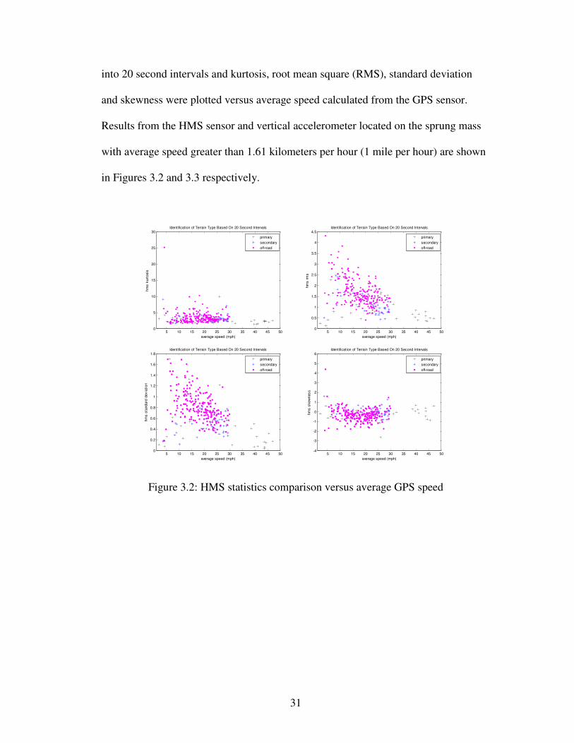
31

into 20 second intervals and kurtosis, root mean square (RMS), standard deviation

and skewness were plotted versus average speed calculated from the GPS sensor.

Results from the HMS sensor and vertical accelerometer located on the sprung mass

with average speed greater than 1.61 kilometers per hour (1 mile per hour) are shown

in Figures 3.2 and 3.3 respectively.

Figure 3.2: HMS statistics comparison versus average GPS speed

5 10 15 20 25 30 35 40 45 500

5

10

15

20

25

30Identification of Terrain Type Based On 20 Second Intervals

average speed (mph)

hm

s k

urt

osis

primary

secondary

off-road

5 10 15 20 25 30 35 40 45 500

0.5

1

1.5

2

2.5

3

3.5

4

4.5Identification of Terrain Type Based On 20 Second Intervals

average speed (mph)

hm

s r

ms

primary

secondary

off-road

5 10 15 20 25 30 35 40 45 500

0.2

0.4

0.6

0.8

1

1.2

1.4

1.6

1.8Identification of Terrain Type Based On 20 Second Intervals

average speed (mph)

hm

s s

tandard

devia

tion

primary

secondary

off-road

5 10 15 20 25 30 35 40 45 50-4

-3

-2

-1

0

1

2

3

4

5

6Identification of Terrain Type Based On 20 Second Intervals

average speed (mph)

hm

s s

kew

nes

s

primary

secondary

off-road

32

Figure 3.3: Accelerometer statistics comparison versus average GPS speed

Careful examination of Figures 3.2 and 3.3 show accelerometer RMS,

standard deviation and kurtosis provide good differentiation of primary, secondary

and off-road courses when plotted versus average speed. As would be expected of

vertical accelerometer data based on terrain, the RMS and standard deviation values

are nearly identical. This is due to the fact that when the mean is zero, the standard

deviation and RMS statistics are identical. Gravitational acceleration was zeroed out

of this data so the mean is very near zero for most samples. Skewness values for both

sensors showed fairly random distribution of the data, and HMS sensor RMS,

standard deviation and kurtosis showed less separation than accelerometer statistics.

Accelerometer RMS, standard deviation and kurtosis were selected as candidate

statistics for the terrain identification algorithms.

5 10 15 20 25 30 35 40 45 500

5

10

15

20

25

30Identification of Terrain Type Based On 20 Second Intervals

average speed (mph)

accele

rom

ete

r kurt

osis

primary

secondary

off-road

5 10 15 20 25 30 35 40 45 500

0.05

0.1

0.15

0.2

0.25

0.3

0.35

0.4

0.45Identification of Terrain Type Based On 20 Second Intervals

average speed (mph)

accele

rom

ete

r rm

s

primary

secondary

off-road

5 10 15 20 25 30 35 40 45 500

0.05

0.1

0.15

0.2

0.25

0.3

0.35

0.4

0.45Identification of Terrain Type Based On 20 Second Intervals

average speed (mph)

accele

rom

ete

r sta

ndard

devia

tion

primary

secondary

off-road

5 10 15 20 25 30 35 40 45 50-1

-0.5

0

0.5

1

1.5

2

2.5

3

3.5Identification of Terrain Type Based On 20 Second Intervals

average speed (mph)accele

rom

ete

r skew

ness

primary

secondary

off-road

33

3.3.2 Evaluation Procedure

In order for the statistics to be compared numerically, it was necessary to

develop a repeatable, automated process to divide the state-space into regions of

primary, secondary and off-road terrains. In addition, this process would need to take

into account the unequal number of tested data points in each category. The first step

taken was to remove data points where the average speed was below 1.61 kilometers

per hour (1 mile per hour) from the data set. It was assumed that points where the

average speed was below 1.61 kilometers per hour (1 mile per hour) were indicative

of times when the vehicle was mainly stationary and would not be subject to terrain

induced loading. A least squares fit linear regression was performed on the

remaining data in each category and the standard deviation of the residuals from the

fit were calculated. Boundaries were set by determining the point between the two

bordering regression lines where the number of residual standard deviations from

each corresponding regression line was equal. The equation for the line through these

points was found and used as the boundary between regions. Figures 3.4 and 3.5

illustrate this procedure.

34

Figure 3.4: Calculating standard deviation of residuals from linear fit

Figure 3.5: Automated procedure for defining terrain regions

0 10 20 30 40 50 60 700

0.05

0.1

0.15

0.2

0.25

0.3

0.35

0.4

0.45

0.5Identification of Terrain Type Based On 20 Second Intervals

average speed (mph)

accele

rom

ete

r rm

s

train primary

train secondary

train off-road

secondary

primary

off-road

0 10 20 30 40 50 60 700

0.05

0.1

0.15

0.2

0.25

0.3

0.35

0.4

0.45

0.5Identification of Terrain Type Based On 20 Second Intervals

average speed (mph)

accele

rom

ete

r rm

s

train primary

train secondary

train off-road

secondary

primary

off-road

0 10 20 30 40 50 60 70

-0.2

-0.1

0

0.1

0.2

Secondary Residuals from Estimate

average speed (mph)

acce

lero

mete

r rm

s

0 10 20 30 40 50 60 70

-0.2

-0.1

0

0.1

0.2

Off-Road Residuals from Estimate

average speed (mph)

acc

ele

rom

ete

r rm

s

0 10 20 30 40 50 60 70

-0.2

-0.1

0

0.1

0.2

Primary Residuals from Estimate

average speed (mph)

acc

ele

rom

ete

r rm

s

35

Data that fell below the lines defining the terrain boundaries were considered

primary terrain for this model. Data above the lines were defined as off-road terrain

and the remaining data was considered secondary terrain. This ensured the regions

were mutually exclusive within the reasonable state-space. Terrain boundaries did

not overlap for the data studied here, but this may become an issue as the model is

applied to other vehicles, sensors, or statistics.

Data from the training set were used to calculate terrain boundaries. Testing

data were then used to objectively test the accuracy of the boundary. For reporting

purposes, terrain identification accuracy was calculated as the average of the ratio of

intervals correctly identified in each category to the number of intervals measured in

each category.

3.3.3 Sample Window Size

One of the critical parameters deemed worthy of investigation for this model

was the length of time used for each data point. Speed was observed to change

significantly over sections longer than 20 seconds for many of the courses used in this

analysis. Average speed was thought to be misleading for longer time segments, so

20 seconds was selected as the upper limit for sample windows investigated. A lower

limit was set at 0.5 seconds. A sample window shorter than 0.5 seconds was expected

to contain too little terrain information to provide good statistical measures. An

initial inspection performed visually of different sample window sizes did not show

obvious superiority of one sample rate. Thus, the automated procedure was used to

36

evaluate the accuracy of terrain identification for sample window sizes ranging from

0.5 to 20 seconds.

3.4 Fatigue Estimation

In order to evaluate accuracy of fatigue damage estimations, a representative

usage made up of the available terrain types was necessary to compare the variables

equitably. Requirements documents indicate a predicted usage in terms of primary,

secondary and off-road courses for each variant of the demonstration vehicle.

Durability tests for army combat vehicles are commonly 32,200 kilometers (20,000

miles) in length following and were assumed to follow the expected terrain profile for

the most common variant. High fidelity fatigue damage estimates based on measured

strain data for each of the courses were scaled based on Miner’s damage summation

rule (Miner 1945) which relates number of cycles nk, and number of cycles to failure

Nk to damage D.

DN

nm

k k

k =∑=1

(1)

High fidelity fatigue damage predictions were made for the training and testing data

sets undergoing a 32,200 kilometer (20,000) mile durability test.

A model similar to Miner’s damage summation rule was developed for

predicting fatigue damage from terrain exposure. This model relates the number of

samples of exposure to one of the three terrain types sk and the predicted number of

samples to failure Sk to damage D.

37

DS

s

k k

k =∑=

3

1

(2)

The inverse of the predicted number of cycles to failure is the expected damage per

sample. Expected damage per sample is the average fatigue damage per exposure

window from the training data set. Values for 20 second segments are shown in

Table 3.1. Segments that fell in the primary, secondary, and off-road terrain regions

were scaled using Miner’s damage summation rule to fit the durability profile and an

estimated damage D was calculated and compared to the high fidelity fatigue model

for the testing data sets. Accuracy of the fatigue damage estimation was calculated as

the ratio of damage predicted using the terrain identification model scaled to a 32,200

kilometer (20,000) mile durability test to the damage predicted from the high fidelity

fatigue model scaled to a 32,200 kilometer (20,000) mile durability test.

3.5 Results

Terrain identification and fatigue estimates were made based on accelerometer

RMS, standard deviation and kurtosis for various sample window sizes. Training

data sets were used to develop terrain identification regions and independent data sets

were used for testing purposes. Results from the test data sets are plotted in Figures

3.6 and 3.7. Terrain identification accuracy generally increased with longer sample

window sizes. Accelerometer RMS was shown to be most accurate at terrain

identification, with all values between 32% and 81% accurate. Fatigue damage

estimates were less accurate. Accuracy varied between 239% and 540% of that

predicted by the high fidelity fatigue model.

38

Figure 3.6. Terrain identification accuracy for various statistics

Figure 3.7. Fatigue estimate accuracy for various statistics

10-1

100

101

102

0

100

200

300

400

500

600Fatigue Testing Accuracy for Accelerometer

sample window (sec)

accura

cy (

%)

RMS

Standard Deviation

Kurtosis

perfect

10-1

100

101

102

0

10

20

30

40

50

60

70

80

90

100

110Terrain Identification Testing Accuracy for Accelerometer

sample window (sec)

accura

cy (

%)

RMS

Standard Deviation

Kurtosis

perfect

39

One of the major assumptions made in the fatigue damage estimation model

proposed in Equation (2) is that the average fatigue damage is reasonably consistent

between the training and testing data sets for the terrain types. As can be seen in

Table 3.1, this assumption was not entirely accurate. Thus the primary reason that the

fatigue damage estimates were more damaging than predicted by the high fidelity

fatigue estimation was that the off-road terrain used in training the model is

considerably more damaging than that of testing. In order to make a prediction with

accuracy commensurate with the terrain identification accuracy, fatigue damage of

training data needs to be very similar to the data used in testing. Typically, several

courses are used during a durability test to represent each of the terrain types. Using

multiple courses in the fatigue damage estimates would minimize course specific

events and result in a more accurate fatigue prediction. The number of samples until

failure for each terrain could be adjusted as additional test data is collected or as

failures occur during fielded usage.

3.6 Conclusions

A simple model was developed that identifies terrain exposure from robust

sensors located at a benign location within a vehicle system. Terrain exposure was

then used to estimate fatigue damage accumulated on a particular component with

reasonable success. A model such as the one described here that estimates fatigue

damage based on terrain exposure is an ideal candidate for use in HUMS applied to

military ground vehicles. Terrain induced loading is the primary failure mechanism

for many of the electronic and mechanical components within a military ground

vehicle system. A single set of sensors and algorithms can provide terrain exposure

40

for an entire vehicle. Estimating fatigue damage accumulated on individual

components is merely a matter of determining scale factors associated with each

terrain type. Thus a large number of components can be monitored with a small set

of robust sensors in benign locations. Computational power and data processing can

be performed by reasonably priced on-board electronics. This permits condition

based maintenance to be performed based on the estimated health of the individual

components, raising the reliability and availability of monitored vehicles. In addition,

as terrain exposure data is collected and archived, higher fidelity estimates of vehicle

usage can be utilized to improve the design of future military vehicle systems.

While the accuracy of the model developed could be improved, results are

within the typical error of fatigue estimates for similar components subjected to

widely varying vibration inputs. Selection of representative terrain was shown to be

critical for accurately training fatigue models. Knowledge of damage rates for each

terrain type or a high fidelity fatigue model applied to representative test data are

essential for accurate fatigue predictions. Further refinement of terrain type and road

conditions tested may provide improved accuracy of terrain identification model.

More complicated models and sensor suites may be necessary for components that are

susceptible to multiple sources of load such as thermal and vibration.

41

Chapter 4: Terrain Identification for Mechanical Components

In order to apply a HUMS to mechanical components on a military ground

vehicle, simplified algorithms that drive terrain exposure from a basic set of sensors

and estimate fatigue damage accumulated on components whose loading comes

primarily from terrain have been developed. Inputs and statistical parameters are

evaluated for this model based on accuracy of terrain identification and quality of

fatigue prediction on an example component. The remainder of material in Chapter 4

is presented as it was formatted for submission to the Journal of the Institute of

Environmental Sciences and Technology and contains repeated background

information. To avoid repeated information, readers should skip to section 4.2.

4.1 Background

Reliability of military vehicle systems is being driven upward to mitigate life

cycle cost and improve operational availability and readiness. New requirements for

functionality and performance are resulting in increasingly complex vehicle systems.

In order to address these conflicting issues, novel ways to improve reliability and

readiness are needed. One method that is favored in the Department of Defense is the

inclusion of a Health and Usage Monitoring System or HUMS within a vehicle

platform. HUMS can be practically defined as a system of sensors, processors and

algorithms that give an indication of remaining component life. These systems

provide an indication of the usage of an individual vehicle and the effect of the

environmental factors on specific monitored components. The resulting data is

processed and provides information to operators, maintainers, and mission planning

42

personnel as to which components should be serviced, which vehicles have the lowest

probability of failure during a mission, and what the past usage of the vehicle has

been. With good management, this information can be used to increase availability

and reliability, while decreasing overall maintenance and system cost.

The costs associated with development and purchasing, along with the

detailed information of the system necessary to perform health and usage monitoring,

have limited application to very expensive systems that are operated over long time

spans. Applications of HUMS to vehicles have been primarily performed on fixed-

wing aircraft (Anon 2004, Trammel 1997, Hunt 2001) and rotorcraft (Ellerbrock

1999, Evans 2002, Bechhoefer 2004, Gordon 1991.) Other notable applications

include an artillery system (Araiza 2002), manufacturing facility (Li 1995) and power

plant (Jarrell 2006.) The life cycle cost and safety issues associated with these

applications justify the development of complicated HUMS. The development and

unit cost of a HUMS applied to a military land vehicle would need to be much less.

The cost to develop a military ground vehicle system is often several orders of

magnitude less than that of an aircraft, so expenditures for the development of a

HUMS would have to be reduced by a relative proportion. In addition, cost of the

HUMS could not be a significant portion of the vehicle cost. Redesign of

components or replacement of the entire system may be a preferred alternative if the

unit cost of a HUMS is prohibitive.

Some relatively low-cost HUMS have been developed for an elevator system

(Yan 2005) and computer server applications (Schuster 2004). The specialized load

cases and failure mechanisms in these examples limit the relevance to military ground

43

vehicle platforms. A survey of HUMS technologies for electronics has been

performed, but many of the techniques discussed provide health and usage

information specific to a single device, board or component (Vichare 2006.) The

additional cost for hardware and development may be difficult to justify for a military

ground vehicle if insight is limited to a specific component, board or even device.

One of the few instances of developing a HUMS for a ground vehicle was focused on

the assessment of vibration for rotating components within the turbine engine of a M1

Abrams tank (Greitzer 2002.) This work involved monitoring the rotating

components for indications of imminent failure. A model based on detecting

precursors to failure requires detailed characterization of damage tolerant components

and is not applicable or justifiable from a cost standpoint to many of the other

components of a ground vehicle system. A generalized model is needed that could

provide inputs into a large number of inexpensive components.

A HUMS applied to a military ground vehicle would also require sensors

reliable enough that the HUMS would not contribute significantly to the total

platform malfunctions. Rough terrain, extreme temperature fluctuations, dust and

moisture are all commonly experienced on military ground vehicle systems and can

be damaging to the sensors. Many of the sensors available for use in aircraft, plant,

or electronic applications would not survive long in this field environment. Frequent

need for replacement or calibration would counter the goal of increasing durability

and readiness, while decreasing the logistics footprint of the platform. In order for

these environmental hazards to be minimized, a limited set of robust sensors must be

utilized for the HUMS.

44

Another key element for the application of a HUMS to a ground vehicle is that

the system must be based on simple algorithms whose computation can be performed

on-board the vehicle. Calculations on the type of data required for the accurate

estimation of fatigue in addition to the error-checking algorithms and digitization

requires significant on-board computational capabilities, but the bandwidth required

for continuous raw data transfer or the unprocessed data storage of long missions

makes off-vehicle processing unfeasible. Algorithms for individual components

must remain simple to allow multiple components to be monitored with inexpensive

hardware.

The objective of this research was to develop a method for the creation and

tuning of algorithms appropriate for a HUMS applied to a military land vehicle

platform. The method developed was designed to be generic such that it could be

applied to any mechanical component subjected primarily to terrain induced loading.

A baseline physics of failure analysis was performed on an example component and

used to demonstrate that the proposed HUMS algorithms are appropriate and provide

suitably accurate fatigue predictions (See Appendix A).

4.2 Demonstration Vehicle and Example Component

An eight wheeled Army vehicle similar to the one shown in Figure 4.1 was

utilized as the demonstration vehicle for this research. Data were collected from

candidate sensors for the HUMS. These included an accelerometer on the sprung

mass of the vehicle, Global Positioning Satellite (GPS) data, and J1708 data bus

sensors. Strain data was also collected near a welded connection on a critical steering

component over multiple courses at the Yuma Proving Ground. A high-fidelity

45

fatigue analysis was performed on the strain data for each course using the

commercially available software.

Figure 4.1: Army eight wheeled vehicle system

Figure 4.2 shows an example component with its welded joint. A physics of

failure analysis was performed to determine the fatigue life for the component (See

Appendix A). Root cause of failure was determined to be caused, in part, by terrain

specific loading. The steering components are also subjected to other forces such as

turning loads, but fatigue damage to this component was traced to the terrain induced

loading. Further details regarding the example component have been intentionally

obscured to minimize available information on failure modes of military equipment.

It is the purpose of this work to present the method for application of remaining life

prognostics algorithms and details of the exact component are unnecessary.

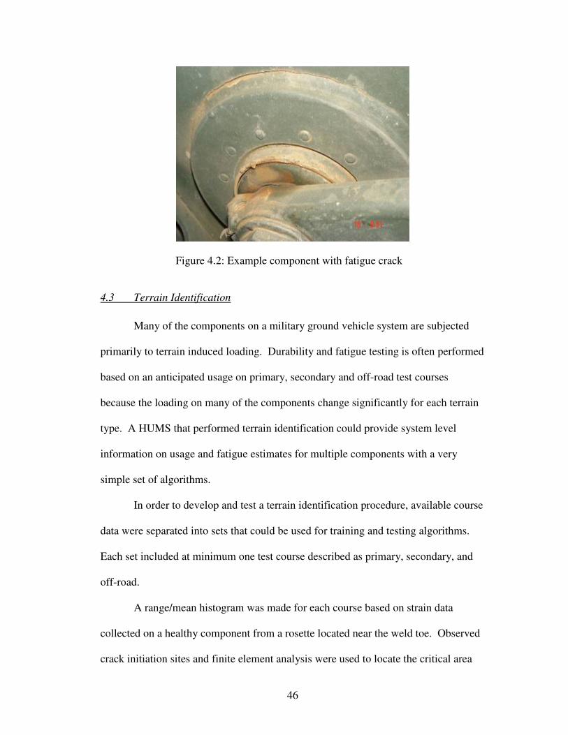
46

Figure 4.2: Example component with fatigue crack

4.3 Terrain Identification

Many of the components on a military ground vehicle system are subjected

primarily to terrain induced loading. Durability and fatigue testing is often performed

based on an anticipated usage on primary, secondary and off-road test courses

because the loading on many of the components change significantly for each terrain

type. A HUMS that performed terrain identification could provide system level

information on usage and fatigue estimates for multiple components with a very

simple set of algorithms.

In order to develop and test a terrain identification procedure, available course

data were separated into sets that could be used for training and testing algorithms.

Each set included at minimum one test course described as primary, secondary, and

off-road.

A range/mean histogram was made for each course based on strain data

collected on a healthy component from a rosette located near the weld toe. Observed

crack initiation sites and finite element analysis were used to locate the critical area

47

for fatigue. Fatigue damage accumulated and life predictions were then made for

each course using the British Weld Standard BS 7608 (1993.) Life predictions were

verified anecdotally based on failures and usage rates of fielded systems. Table 4.1

provides the results of the high fidelity fatigue analysis of measured strain data.

Fatigue damage calculated for the entire course was divided by the number of twenty

second intervals where average speed was above 1.61 kilometers per hour (1 mile per

hour) that were necessary to traverse the courses in each category.

Table 4.1: Average fatigue damage per 20 seconds exposure

Terrain Type Training Data Set Testing Data Set

Primary 6.25E-07 2.82E-07

Secondary 1.35E-04 6.10E-06

Off-Road 2.30E-04 2.70E-05

4.3.1 Sample Statistics

In order to identify terrain, it was necessary to develop a simple method to

determine terrain type from potential HUMS sensors. A sprung mass accelerometer

was selected as a candidate likely to be indicative of terrain type. Training data from

the potential HUMS sensor was sectioned into 20 second intervals and kurtosis, root

mean square (RMS), standard deviation and skewness were plotted versus average

speed calculated from the GPS sensor. Results from the vertical accelerometer

located on the sprung mass with average speed greater than 1.61 kilometers per hour

(1 mile per hour) are shown in Figure 4.3.

48

Figure 4.3: Accelerometer statistics comparison versus average GPS speed

Careful examination of Figure 4.3 shows accelerometer RMS, standard

deviation and kurtosis provide differentiation of primary, secondary and off-road

courses when plotted versus average speed. As would be expected of vertical

accelerometer data based on terrain, the RMS and standard deviation values are

nearly identical. This is due to the fact that when the mean is zero, the standard

deviation and RMS statistics are identical. Gravitational acceleration was zeroed out

of this data so the mean is very near zero for most samples. Skewness values showed

fairly random distribution of the data. Accelerometer RMS, standard deviation and

kurtosis were selected as potential candidate statistics for the terrain identification

algorithms.

5 10 15 20 25 30 35 40 45 500

5

10

15

20

25

30Identification of Terrain Type Based On 20 Second Intervals

average speed (mph)

accele

rom

ete

r kurt

osis

primary

secondary

off-road

5 10 15 20 25 30 35 40 45 500

0.05

0.1

0.15

0.2

0.25

0.3

0.35

0.4

0.45Identification of Terrain Type Based On 20 Second Intervals

average speed (mph)

accele

rom

ete

r rm

s

primary

secondary

off-road

5 10 15 20 25 30 35 40 45 500

0.05

0.1

0.15

0.2

0.25

0.3

0.35

0.4

0.45Identification of Terrain Type Based On 20 Second Intervals

average speed (mph)

accele

rom

ete

r s

tandard

devia

tion

primary

secondary

off-road

5 10 15 20 25 30 35 40 45 50-1

-0.5

0

0.5

1

1.5

2

2.5Identification of Terrain Type Based On 20 Second Intervals

average speed (mph)accele

rom

ete

r skew

ness

primary

secondary

off-road

5 10 15 20 25 30 35 40 45 500

5

10

15

20

25

30Identification of Terrain Type Based On 20 Second Intervals

average speed (mph)

accele

rom

ete

r kurt

osis

primary

secondary

off-road

5 10 15 20 25 30 35 40 45 500

0.05

0.1

0.15

0.2

0.25

0.3

0.35

0.4

0.45Identification of Terrain Type Based On 20 Second Intervals

average speed (mph)

accele

rom

ete

r rm

s

primary

secondary

off-road

5 10 15 20 25 30 35 40 45 500

0.05

0.1

0.15

0.2

0.25

0.3

0.35

0.4

0.45Identification of Terrain Type Based On 20 Second Intervals

average speed (mph)

accele

rom

ete

r s

tandard

devia

tion

primary

secondary

off-road

5 10 15 20 25 30 35 40 45 50-1

-0.5

0

0.5

1

1.5

2

2.5Identification of Terrain Type Based On 20 Second Intervals

average speed (mph)accele

rom

ete

r skew

ness

primary

secondary

off-road

49

4.3.2 Evaluation Procedure

In order for the statistics to be compared numerically, it was necessary to develop a

repeatable, automated process to divide the state-space into regions of primary,

secondary and off-road terrains. In addition, this process would need to take into

account the unequal number of tested data points in each category. The first step

taken was to remove data points where the average speed was below 1.61 kilometers

per hour (1 mile per hour) from the data set. It was assumed that points where the

average speed was below 1.61 kilometers per hour (1 mile per hour) were indicative

of times when the vehicle was mainly stationary and not subject to terrain induced

loading. A least squares fit linear regression was performed on the remaining data in

each category and the standard deviation of the residuals from the fit were calculated.

Boundaries were set by determining the point between the two bordering regression

lines where the number of residual standard deviations from each corresponding

regression line was equal. The equation for the line through these points was found

and used as the boundary between regions. Figures 4.4 and 4.5 illustrate this

procedure.

50

Figure 4.4: Calculating standard deviation of residuals from linear fit

Figure 4.5: Automated procedure for defining terrain regions

0 10 20 30 40 50 60 700

0.05

0.1

0.15

0.2

0.25

0.3

0.35

0.4

0.45

0.5Identification of Terrain Type Based On 20 Second Intervals

average speed

accele

rom

ete

r rm

s

train primary

train secondary

train off-road

secondary

primary

off-road

0 10 20 30 40 50 60 700

0.05

0.1

0.15

0.2

0.25

0.3

0.35

0.4

0.45

0.5Identification of Terrain Type Based On 20 Second Intervals

average speed

accele

rom

ete

r rm

s

train primary

train secondary

train off-road

secondary

primary

off-road

0 10 20 30 40 50 60 70 80

-0.2

-0.1

0

0.1

0.2

Primary Residuals from Estimate

average speed (mph)

accele

rom

ete

r rm

s

0 10 20 30 40 50 60 70 80

-0.2

-0.1

0

0.1

0.2

Secondary Residuals from Estimate

average speed (mph)

accele

rom

ete

r rm

s

0 10 20 30 40 50 60 70

-0.2

-0.1

0

0.1

0.2

Off-Road Residuals from Estimate

average speed (mph)

accele

rom

ete

r rm

s

0 10 20 30 40 50 60 70 80

-0.2

-0.1

0

0.1

0.2

Primary Residuals from Estimate

average speed (mph)

accele

rom

ete

r rm

s

0 10 20 30 40 50 60 70 80

-0.2

-0.1

0

0.1

0.2

Secondary Residuals from Estimate

average speed (mph)

accele

rom

ete

r rm

s

0 10 20 30 40 50 60 70

-0.2

-0.1

0

0.1

0.2

Off-Road Residuals from Estimate

average speed (mph)

accele

rom

ete

r rm

s

51

Data that fell below the lines defining the terrain boundaries were considered

primary terrain for this model. Data above the lines were defined as off-road terrain

and the remaining data were considered secondary terrain. This ensured the regions

were mutually exclusive within the reasonable state-space. Terrain boundaries did

not overlap for the data studied here, but this may become an issue as the model is

applied to other vehicles, sensors, or statistics.

Data from the training set were used to calculate terrain boundaries. Testing

data were then used to objectively test the accuracy of the boundary. For reporting

purposes, terrain identification accuracy was calculated as the average of the ratio of

intervals correctly identified in each category to the number of intervals measured in

each category.

4.3.3 Sample Window Size

One of the critical parameters deemed worthy of investigation for this model

was the length of time used for each data point. Speed was observed to change

significantly over sections longer than 20 seconds for many of the courses used in this

analysis. Average speed was thought to be misleading for longer time segments, so

20 seconds was selected as the upper limit for sample windows investigated. A lower

limit was set at 0.5 seconds. A sample window shorter than 0.5 seconds was expected

to contain too little terrain information to provide good statistical measures. An

initial inspection performed visually of different sample window sizes did not show

obvious superiority of one sample size. Thus, the automated procedure was used to

evaluate the accuracy of terrain identification for sample window sizes ranging from

0.5 to 20 seconds.

52

4.4 Fatigue Estimation

In order to evaluate accuracy of fatigue damage estimations, a representative

usage made up of the available terrain types was necessary to compare the variables

equitably. Requirements documents indicate a predicted usage in terms of primary,

secondary and off-road courses for each variant of the demonstration vehicle.

Durability tests for army combat vehicles are commonly 32,200 kilometers (20,000

miles) in length and are assumed to follow the expected terrain profile for the most

common variant. High fidelity fatigue damage estimates based on measured strain

data for each of the courses were scaled based on Miner’s damage summation rule

(Miner 1945) which relates number of cycles nk, and number of cycles to failure Nk to

damage D.

DN

nm

k k

k =∑=1

(1)

High fidelity fatigue damage predictions were made for the training and testing data

sets undergoing a 32,200 kilometer (20,000) mile durability test.

A model similar to Miner’s damage summation rule was developed for

predicting fatigue damage from terrain exposure. This model relates the number of

samples of exposure to one of the three terrain types sk and the predicted number of

samples to failure Sk to damage D.

DS

s

k k

k =∑=

3

1

(2)

53

The inverse of the predicted number of cycles to failure is the expected damage per

sample. Expected damage per sample is the average fatigue damage per exposure

window from the training data set. Values for 20 second segments are shown in

Table 4.1. Segments that fell in the primary, secondary, and off-road terrain regions

were scaled using Miner’s damage summation rule to fit the durability profile and an

estimated damage D was calculated and compared to the high fidelity fatigue model

for the testing data sets. Accuracy of the fatigue damage estimation was calculated as

the ratio of damage predicted using the terrain identification model scaled to a 32,200

kilometer (20,000 mile) durability test to the damage predicted from the high fidelity

fatigue model scaled to a 32,200 kilometer (20,000 mile) durability test.

4.5 Results

Terrain identification and fatigue estimates were made based on

accelerometer RMS, standard deviation and kurtosis for various sample window

sizes. Training data sets were used to develop terrain identification regions and

independent data sets were used for testing purposes. Results from the test data sets

are plotted in Figures 4.6 and 4.7. Terrain identification accuracy based on RMS and

standard deviation generally increased with longer sample window sizes. Kurtosis

showed no clear trend based on sample window size. Accelerometer standard

deviation was shown to be most accurate at terrain identification, with all values

between 46% and 55% accurate. Fatigue damage estimates were less accurate.

Accuracy from accelerometer standard deviation varied between 450% and 682% of

that predicted by the high fidelity fatigue model.

54

Figure 4.6. Terrain identification accuracy for various statistics

Figure 4.7. Fatigue estimate accuracy for various statistics

10-1

100

101

102

0

100

200

300

400

500

600

700

800

900

1000Fatigue Testing Accuracy for Accelerometer

sample window (sec)

accura

cy (

%)

RMS

Standard Deviation

Kurtosis

perfect

10-1

100

101

102

0

10

20

30

40

50

60

70

80

90

100

110Terrain Identification Testing Accuracy for Accelerometer

sample window (sec)

accura

cy (

%)

RMS

Standard Deviation

Kurtosis

perfect

55

In order for the fatigue damage estimation model proposed in Equation (2) to

provide accurate projections, it is necessary that the average fatigue damage is

reasonably consistent between the training and testing data sets for the terrain types.

As can be seen in Table 4.1, this assumption was not entirely accurate. Primary and

off road terrain provided relatively good matches, but secondary varied significantly

between the training and testing data sets. Thus the main reason that the fatigue

damage estimates were more damaging than predicted by the high fidelity fatigue

estimation was that the secondary terrain used in training the model is considerably

more damaging than that of testing. In order to make a prediction with accuracy

commensurate with the terrain identification accuracy, fatigue damage of training

data needs to be very similar to the data used in testing. Typically, several courses

are used during a durability test to represent each of the terrain types. Using multiple

courses in the fatigue damage estimates would minimize course specific events and

result in a more accurate fatigue prediction. The number of samples until failure for

each terrain could be adjusted as additional test data is collected or as failures occur

during fielded usage.

4.6 Conclusions

A simple model was developed that identifies terrain exposure from robust

sensors located at a benign location within a vehicle system. Terrain exposure was

then used to estimate fatigue damage accumulated on a particular component with

reasonable success. A model such as the one described here that estimates fatigue

damage based on terrain exposure is an ideal candidate for use in HUMS applied to

56

military ground vehicles. Terrain induced loading is the primary failure mechanism

for many of the electronic and mechanical components within a military ground

vehicle system. A single set of sensors and algorithms can provide terrain exposure

for an entire vehicle. Estimating fatigue damage accumulated on individual

components is merely a matter of determining scale factors associated with each

terrain type. Thus a large number of components can be monitored with a small set

of robust sensors in benign locations. Computational power and data processing can

be performed by reasonably priced on-board electronics. This permits condition

based maintenance to be performed based on the estimated health of the individual

components, raising the reliability and availability of monitored vehicles. In addition,

as terrain exposure data is collected and archived, higher fidelity estimates of vehicle

usage can be utilized to improve the design of future military vehicle systems.

While the accuracy of the model developed could be improved, results are

within the typical error of fatigue estimates for similar components subjected to

widely varying vibration inputs. Selection of representative terrain was shown to be

critical for accurately training fatigue models. Knowledge of damage rates for each

terrain type or a high fidelity fatigue model applied to representative test data are

essential for accurate fatigue predictions. Further refinement of terrain type and road

conditions tested may provide improved accuracy of terrain identification model.

More complicated models and sensor suites may be necessary for components that are

susceptible to multiple sources of load.

57

Chapter 5: Acceleration-Based Strain Estimation

This chapter defines a set of more computationally complex algorithms that

use measured acceleration to predict strain and fatigue damage that is suitable for

special load cases where acceleration waveforms can be shown to be similar to strain.

The feasibility of using vibratory inputs from an accelerometer to make component

fatigue predictions for a military wheeled vehicle system is explored and the use of

limited subsets of data for algorithm training are evaluated. An example component

is used to demonstrate that the proposed HUMS algorithms are appropriate and

provide suitably accurate fatigue predictions. The remainder of material in Chapter 5

is presented as it was formatted for submission to the Journal of the Institute of

Environmental Sciences and Technology and contains repeated background

information. To avoid repeated information, readers should skip to the last two

paragraphs in section 5.1.

5.1 Background

Reliability, availability and maintainability (RAM) are critical requirements

for military ground vehicle programs. These requirements help to ensure that a

system meets user needs in a timely manner and at a reasonable price. The increasing

complexity of military vehicle systems coupled with the user’s desire for expanded

performance is reducing design margins and making RAM requirements more

difficult to achieve. Innovative technologies need to be developed and applied to

maintain high performance materiel at reasonable prices. One method that is being

promoted in the Department of Defense is the inclusion of a Health and Usage

58

Monitoring System or HUMS within a vehicle platform. HUMS can be practically

defined as a system of sensors, processors and algorithms that give an indication of

remaining component life. These systems provide an indication of the usage of

individual vehicles and the effect of the environmental factors on specific monitored

components. The resulting data are processed and provide information to operators,

maintainers, and mission planning personnel as to which components should be

serviced, which vehicles have the lowest probability of failure during a mission, and

what the past usage of the vehicle has been. With good management, this information

can be used to increase availability and reliability, while decreasing overall

maintenance and system cost.

The costs associated with development and purchasing, along with the

detailed information of the system necessary to perform health and usage monitoring,

typically limit application to critical components within expensive systems that are

subjected to relatively simple environmental and loading conditions and operated

over long time spans. Applications of HUMS to vehicles have been primarily

performed on fixed-wing aircraft (“Prognostics...” 2004, Trammel 1997, Hunt 2001)

and rotorcraft (Ellerbrock 1999, Evans 2002, Bechhoefer 2004, Gordon 1991.) Other

notable examples include a HUMS developed for an artillery system (Araiza 2002),

manufacturing facility (Li 1995) and power plant (Jarrell 2006.) The relevancy of the

techniques and processes developed for these applications to a military ground

vehicle is limited. These examples are exposed to environment and loading

conditions that have significantly less variation than those of a ground vehicle. In

order to address all the relevant load cases on a ground vehicle system, robust

59

engineering models are needed to calculate damage accumulated. Use of these

techniques on a military ground vehicle is also a challenge due to the fact that the life

cycle cost associated with previous applications justify the development of

complicated HUMS. The development and unit cost of a HUMS applied to a military

land vehicle would need to be much less. The cost to develop a military ground

vehicle system is often several orders of magnitude less than that of an aircraft, so

expenditures for the development of a HUMS would have to be reduced by a relative

proportion. In addition, cost of the HUMS could not be a significant portion of the

vehicle cost. Redesign of components or replacement of the entire system may be a

preferred alternative if the unit cost of a HUMS is prohibitive.

One previous instance of a HUMS applied to a ground vehicle focused on the

damage caused by vibration of rotating components within the turbine engine of an

M1 Abrams tank (Greitzer 2002.) Techniques developed for aircraft could be directly

applied to this work which involved monitoring rotating components for indications

of imminent failure, but detailed characterization of damage tolerant components is

necessary to detect precursors to failure. The testing or analytical burden required to

identify precursors to failure and the limitation of the information provided to a single

failure mode within a single subsystem makes such applications hard to justify from a

cost standpoint for even the most expensive ground vehicles.

There have been instances where a HUMS was developed for relatively low-

cost applications such as an elevator system (Yan 2005) and computer servers

(Schuster 2004.) A survey of HUMS technologies for electronics has been

performed, and many of the techniques discussed provide health and usage

60

information specific to a single device, board or component (Vichare 2006.) The

specialized load cases and failure mechanisms in these examples limit the relevance

to items on military ground vehicle platforms beyond electronics, however these

examples are successful in demonstrating the practicality of applying a HUMS for

specific components in a low-cost application.

A general set of algorithms for application of HUMS to a military ground

vehicle system was developed based on the relationship of fatigue damage to terrain

type (see Chapter 4.) Durability and fatigue testing are often performed based on an

anticipated usage on primary, secondary and off-road terrains because the loading on

many of the components changes significantly for each terrain type. These

algorithms take advantage of the similarity of damage rates within each terrain type to

estimate fatigue damage accumulated on individual components. One of the major

advantages of this system is that a very simple set of sensors and algorithms provide

damage estimates for multiple components. This effectively spreads the

developmental and unit cost of the HUMS across many components. Accuracy of

fatigue damage predicted from terrain identification algorithms varied by a factor of

4.5 and 6.8 to damage predicted by a high fidelity fatigue model. These results are

within the typical error of fatigue estimates for similar components subjected to

widely varying vibration inputs, but accuracy was shown to be highly dependent on

identifying a fatigue damage per exposure time scale factor that is representative for

all conditions within a terrain type. This requires significant testing on multiple

courses that would represent the full range of scenarios that a military vehicle would

encounter. The desire for a more accurate fatigue estimate and the ability to

61

minimize algorithm training data required may justify more complex algorithms for

some components. A model that could work in concert with terrain identification

model to provide enhanced fatigue damage predictions while minimizing algorithm

training data, would be useful for components deemed critical or safety related.

One of the major difficulties in application of a HUMS is the limitation

caused by sensors. Any sensors used need to be reliable enough that the HUMS

would not contribute significantly to the total platform malfunctions. Rough terrain,

extreme temperature changes, dust and large fluctuations in humidity are all

commonly experienced on military vehicle systems and can be damaging to a HUMS.

Sensors are especially sensitive to these effects. Constant replacement or calibration

requiring human interaction would be counter to the goals of increasing durability and

readiness, while decreasing the logistics footprint of the platform. Strain

measurements are desirable as an input to fatigue damage estimation models.

However, the common method of measuring strain with adhesively bonded strain

gauges is fraught with difficulties. Strain gauges are sensitive to temperature

variations, and bonding can be an issue if expected to last the life of the component.

Accelerometers are another common sensor which gives an indication of terrain

induced loading. Accelerometers are relatively durable and reasonable in cost which

makes them an ideal candidate for use in a HUMS applied to a military ground

vehicle system.

The objectives of this research are to investigate the feasibility of using

vibratory inputs from an accelerometer to make component fatigue predictions for a

military wheeled vehicle system and examine methods to improve HUMS predictions

62

for specific components. Use of limited subsets of data for algorithm training will

also be evaluated. A baseline physics of failure analysis was performed on an

example component and used to demonstrate that the proposed HUMS algorithms are

appropriate and provide suitably accurate fatigue predictions (See Appendix A).

5.2 Demonstration Vehicle and Component

The hydraulic reservoir shown in Figure 5.1 was selected as a demonstration

component for this study. This reservoir supplies fluid for a number of hydraulic

subsystems within a wheeled army vehicle system. Fatigue cracking was noted

during automotive testing and the root cause of failure was determined to be terrain

induced vibration.

Figure 5.1: Hydraulic reservoir in Army wheeled vehicle

Instrumented data were taken from a series of test courses and obstacles

determined to be damaging to the hydraulic reservoir at an Army facility. These

63

included obstacles made up of 8, 10, 12 and 16 inch half rounds affixed to a flat road

course, a series of gravel courses with periodic bumps to give defined root mean

square values, and two severe off-road courses. Acceleration data were collected

from several locations on the vehicle and reservoir, and strain data were collected for

major failure locations. A high fidelity fatigue analysis was performed on the strain

data for each course using commercially available software and stress life curves for

weldments defined in the European Recommendations of Aluminum Alloy Structures

Fatigue Design (1992.) Physical validation using shaker table testing based on

measured acceleration showed failures closely matched high fidelity fatigue

estimates. Further details regarding the example component have been intentionally

obscured to minimize available information on failure modes of military equipment.

It is the purpose of this work to present the method for application of remaining life

prognostics algorithms and details of the exact component are unnecessary.

5.3 Waveform Comparison

Calculation of the principal angle during the fatigue analysis of the reservoir

showed that strain in the most critical location was uniaxial along a single rosette leg.

Vertical acceleration induced by terrain was determined to be the principal cause of

failure, so a vertical accelerometer connected to the hull of the demonstration vehicle

was selected for comparison with the critical strain. Figure 5.2 shows samples of the

measured data for each of the course types.

64

2 2.5 3 3.5 4 4.5 5 5.5 6-2

-1

0

1

2Obstacle

time (s)

accel (g

)

2 2.5 3 3.5 4 4.5 5 5.5 6-500

0

500

1000

1500

time (s)

str

ain

(m

icro

str

ain

)

20 25 30 35-2

-1

0

1

2Periodic

time (s)

accel (g

)

20 25 30 35-500

0

500

1000

time (s)

str

ain

(m

icro

str

ain

)

110 115 120 125 130 135 140-2

-1

0

1

2Off-road

time (s)

accel (g

)

110 115 120 125 130 135 140-500

0

500

1000

time (s)

str

ain

(m

icro

str

ain

)

Figure 5.2: Sample strain and acceleration comparisons

As can be seen in Figure 5.2, the overall shape was very similar for the strain

and acceleration measurements. Acceleration measurements appear to have

significantly more high frequency, low amplitude cycles, and acceleration data was

more symmetric around the abscissa than the strain data. Comparisons of fatigue

damage estimates based on strain with and without mean stress correction factors

showed negligible change in predicted life so the level of symmetry was determined

to be not an issue. To determine if correlation exists between the two signals and

whether relative magnitudes were equivalent, Root Mean Square (RMS) strain and

RMS acceleration for 5 second intervals are plotted in Figure 5.3. Interval ranges

65

between 0.5 and 20 seconds were investigated, but 5 second intervals were used to

reduce scatter from wild points or spikes while retaining significantly different RMS

values due to spatial changes in terrain.

0 50 100 150 200 250 300 3500

0.1

0.2

0.3

0.4

0.5

0.6

0.7

0.8RMS Values with 5 Second Window

RMS strain (microstrain)

RM

S a

ccel (g

)

Obstacle

Periodic

Off-road

Figure 5.3: Sample strain and acceleration comparisons

There appears to be a linear correlation between RMS strain and RMS

acceleration for each of the course types. This suggests that there is a relationship

between the strain and acceleration signals and that the magnitude of individual time

segments is proportional.

5.4 Fatigue Estimates

Analysis based on strain data is the most common approach for making

mechanical component fatigue damage estimates. When strain is shown to be

66

uniaxial, estimating damage is relatively simple computationally. Remaining life

estimates can be made using rainflow cycle counting to separate individual stress

cycles, Basquin’s model to evaluate damage for each cycle and Miner’s rule for

damage summation. These algorithms are simple enough to be performed in real time

with modest computational power and provide reasonably accurate results. A mean

stress correction method can be used if significant preload exists, but for cases with

fully reversed cycles and a low offset to stress, a mean stress correction model is an

unnecessary complication.

The major difficulty in making accurate remaining life predictions with a

HUMS is obtaining accurate predictions of the strain cycles at critical locations. To

evaluate accuracy of strain predictions based on accelerometer data, fatigue damage

was calculated from acceleration based models and compared to measured strain

fatigue calculations using the same cycle counting, damage and summation

algorithms. To evaluate the potential for using simple repeatable test courses or

events to predict damage on complex realistic usage, the obstacle and periodic

courses were used for developing relationships between measured acceleration and

strain. The predicted damage on the severe off-road courses was then used to

evaluate the accuracy of the acceleration based fatigue damage versus the measured

strain fatigue damage typically used in high fidelity fatigue models.

5.4.1 Maximum Excursion Scaling

A simple approach for predicting strain from acceleration, assuming that the

peaks that cause fatigue damage are proportional, would be to calculate a scale factor

based on the ratio of the maximum excursion from zero. A small set of large cycles

67

are often major contributors to terrain induced fatigue, so a scaling factor based on

the largest peak was evaluated based on ability to provide accurate fatigue

predictions. The absolute maximums for the sets of obstacle and periodic courses

were calculated for the strain and acceleration data and the ratio of the absolute peak

strain to absolute peak acceleration are the scale factors listed in Table 5.1. The

high fidelity fatigue model based on measured strain predicted average damage per

mile to equal 2.83E-04 for Course 1 and 6.80E-04 for Course 2. Accuracy factor was

defined as the ratio of the strain based damage per mile to the acceleration based

damage per mile in the cases where strain damage was larger than the damage

predicted based on acceleration. In the cases where strain predicted damage was

smaller than acceleration values, the accuracy factor was calculated as the ratio of the

acceleration based damage to the strain based damage. Accuracy factors and

predicted miles to failure based on acceleration data are shown in Table 5.1.

Table 5.1: Maximum excursion scaling

Obstacle Periodic

Scale Factor 362 microstrain/g 268 microstrain/g

Course 1 Acceleration Predicted

Damage/Mile

2.22E-04 6.32E-05

Course 1 Accuracy Factor 1.3 4.5

Course 2 Acceleration Predicted

Damage/Mile

6.63E-04 1.85E-04

Course 2 Accuracy Factor 1.0 3.7

In addition to the accuracy over the total course, it was desired to describe the

accuracy of the model on individual segments. This provides confidence that the

model predictions are unbiased and will not provide a systematic under or over-

68

prediction. Data were segmented into similar size files for each of the off-road

courses. Due to variations in vehicle speed, the course segments varied between 1.7

and 5.3 miles in length. Figure 5.4 graphically presents the strain and acceleration

based average damage predictions for segments of the 15 total miles of Course 1 and

23 total miles of Course 2. The obstacle course based scale factor had relatively

accurate predictions while the periodic course scale factor significantly over predicted

on all of the course segments. Accuracy factors ranged from 1.0 to 1.4 for the

obstacle course based scale factor and from 2.8 to 5.3 for the periodic based scale

factor.

1-1 1-2 1-3 1-4 1-5 1-6 2-1 2-2 2-3 2-4 2-50

0.2

0.4

0.6

0.8

1

1.2

1.4x 10

-3 Obstacle Course Trained Maximum Excursion Model

dam

age/m

ile

offroad course - segment

strain based

accel based

1-1 1-2 1-3 1-4 1-5 1-6 2-1 2-2 2-3 2-4 2-5

0

0.2

0.4

0.6

0.8

1

1.2

1.4x 10

-3 Periodic Course Trained Maximum Excursion Model

dam

age/m

ile

offroad course - segment

strain based

accel based

Figure 5.4: Maximum excursion model for terrain course segments

5.4.2 Fatigue Damage Based Scaling

A second method was evaluated which utilized fatigue damage directly as the

basis for developing the relationship between acceleration and strain. A scale factor

was calculated for each obstacle or periodic course acceleration time history such that

the fatigue damage accumulated was equal to what was predicted from the strain

values. Relative magnitude of individual cycles between strain and acceleration

69

were disregarded in favor of forcing the fatigue damage estimate based on

acceleration for each time history to match the corresponding fatigue damage from

the strain. The average scale factor for the whole group of courses was then tested on

each of the severe off-road courses. Table 5.2 shows results of the analysis.

Table 5.2: Fatigue life scaling

Obstacle Periodic Obstacle &

Periodic

Average Scale Factor 382 microstrain/g 282 microstrain/g 346 microstrain/g

Course 1 Accuracy

Factor

1.0 3.6 1.5

Course 2 Accuracy

Factor

1.2 2.9 1.2

Segments of the two severe off-road test courses were plotted in Figure 5.5.

Periodic course based accelerometer models significantly over-predicted fatigue

damage on each segment. The combination of obstacle and periodic course scale

factors was significantly closer, but the scale factor determined from the obstacle

courses gave the fatigue life estimates closest to the model based on strain

measurements. Accuracy factors ranged from 1.0 to 1.4 for the obstacle course based

scale factor and from 2.8 to 5.3 for the periodic based scale factor. Accuracy factors

ranged from 1.0 to 1.7, 2.2 to 4.2, and 1.0 to 1.8 for the obstacle course, periodic

course, and combination obstacle and periodic course based scale factor respectively.

70

1-1 1-2 1-3 1-4 1-5 1-6 2-1 2-2 2-3 2-4 2-50

0.2

0.4

0.6

0.8

1

1.2

1.4x 10

-3 Obstacle Course Trained Fatigue Damage Model

dam

age/m

ile

offroad course - segment

strain based

accel based

1-1 1-2 1-3 1-4 1-5 1-6 2-1 2-2 2-3 2-4 2-5

0

0.2

0.4

0.6

0.8

1

1.2

1.4x 10

-3 Periodic Course Trained Fatigue Damage Model

dam

age/m

ile

offroad course - segment

strain based

accel based

1-1 1-2 1-3 1-4 1-5 1-6 2-1 2-2 2-3 2-4 2-50

0.2

0.4

0.6

0.8

1

1.2

1.4x 10

-3 Obstacle and Periodic Course Trained Fatigue Damage Model

dam

age/m

ile

offroad course - segment

strain based

accel based

Figure 5.5: Fatigue damage based model for terrain course segments

5.4.3 Potential Improvements

Two processes to reduce the influence of high frequency low range cycles

were evaluated based on their ability to improve fatigue damage estimates. The first

was use of an 8th

order, low pass, Butterworth filter at varying cutoff frequencies to

remove the high frequency cycles. During data collection, accelerometer data was

sampled at 2000 Hz and low pass filtered at 500 Hz, and strain data was sampled at

1000 Hz and low pass filtered down to 100 Hz. As would be expected, frequency

analysis shows that the accelerometer data has more content 100 Hz and above.

Filtering was successful in removing many of the high frequency cycles and tended to

smooth and lower some absolute peaks slightly at high cutoff frequencies. Accuracy

71

of fatigue life predictions showed minimal improvement filtering with cutoff

frequencies between 500 and 100 Hz and a general deterioration in quality of

predictions for cut off frequencies below 100 Hz.

The second process evaluated as a potential improvement was to remove

cycles whose amplitude was below a certain level during rainflow cycle counting.

The removal of ranges below 1 g had little effect on the overall accuracy of the

predictions, generally degrading Course 1 predictions slightly and improving Course

2 predictions by a similar amount. Above 1 g, range removal showed significant

deterioration in quality of all the predictions. Although range removal of cycles does

not significantly improve fatigue, this process does have the benefit of reducing the

computational power necessary to perform the fatigue prediction calculations. In

situations where computational power is limited, this procedure may be worth

pursuing.

5.5 Results

Accurate estimation of strain cycles was determined to be one of the most

critical factors for application of a HUMS fatigue model based on acceleration. Two

simple methods were proposed to determine a scale factor for relating measured

acceleration to strain at a critical location. The scale factor was evaluated based on

the resulting accuracy of fatigue predictions when compared with predictions from a

high fidelity fatigue model using strain at a critical location. Tables 5.1 and 5.2 show

that the accuracy for both models from a fatigue standpoint were an improvement on

those expected from terrain identification models [15]. Of the two methods for

determining a scale factor, fatigue life scaling was determined to provide more

72

accurate fatigue predictions independent of the training course used. In addition,

fatigue damage scaling is more robust due to the fact that it utilizes more data points.

The maximum excursion method could be significantly skewed by a single

unrecognized wild point during training. The fatigue damage scaling method could

also be affected by outliers or spikes in the measurement, but the peaks of all the

cycles that cause damage contribute to the scale factor. Potential improvements to

more closely match the cycle counts between strain and scaled acceleration were

investigated, but determined to provide little improvement to the damage estimation

model.

Two types of simple, repeatable test courses were evaluated based on the

ability to relate acceleration to strain for accurate prediction of fatigue damage on

severe off-road courses. Training on the courses containing half-round obstacles

provided more accurate predictions of fatigue damage than the periodic courses.

Figure 5.3 shows that throughout the RMS strain ranges, obstacle data more closely

match the off-road courses. At high values of strain RMS, which likely contributes

the most to damage estimations, much higher acceleration RMS was measured for the

periodic courses than the obstacle or off-road courses. Under-prediction of strain

would result in the systematic under-prediction of fatigue damage manifested in the

periodic course damage predictions of Figures 5.4 and 5.5. Half round obstacles are

recommended for developing acceleration to fatigue relationships for offroad courses

based on this limited data set. More analysis and testing are needed to verify if

similar events provide suitable relationships for different components, vehicle

systems, and courses.

73

5.6 Conclusions

A model has been proposed to provide remaining life estimation based on

vibratory measurements from an accelerometer. While strain is typically the desired

input to a fatigue model, acceleration sensors are less susceptible to damage from the

military ground vehicle environment and provide more reliable data. Acceleration

measurements may also provide information pertaining to the inputs of multiple

components or multiple locations rather than being limited to a single critical area. A

simple scale factor was determined to be sufficient to relate acceleration and strain for

a sample component. Two methods for the determination of an appropriate scale

factor were evaluated, and calculating the scale factor required to set damage

predictions from the acceleration data equal to strain based predictions at the critical

location for a number of half round obstacles was selected as superior.

It was shown that fatigue damage accuracy for both models and all terrain

courses were improved compared to those expected from terrain identification models

[15]. This model was also shown to require far less training data to develop

relationships suitable for fatigue estimation, but simultaneous strain and acceleration

data are necessary to develop the appropriate scaling and to test the accuracy of

predictions. Computationally, the model developed here is more intensive than a

terrain identification model in that it requires the use of rainflow cycle counting,

Basquin’s model and Miner’s rule for damage summation for each component

monitored. For critical components and safety related equipment, the extra

computational power may be justified for the improved accuracy of the fatigue

predictions.

74

Chapter 6: Identifying Damage Indicators and Physics-Based

Strain Estimation

In this chapter, methods for identifying good indicators of strain from a wide

variety of sensor data for a multiaxial load case were investigated. Physics based

subsystem models are also developed and compared based on the improvement in

fatigue damage prediction capability. A baseline physics of failure analysis was

performed on an example component to evaluate the proposed HUMS algorithms and

demonstrate the accuracy of the resulting fatigue predictions (See Appendix A). The

remainder of material in Chapter 6 is presented as it was formatted for submission in

a technical journal and contains repeated background information. To avoid repeated

information, readers should skip to the last paragraph in section 6.1.

6.1 Background

In a fiscally conscious environment, reliability is always a critical

consideration in the design and manufacture of products. For many items designed to

be used over a long time span, operation and support represents a larger proportion of

the total cost than procurement. Reliability directly affects the logistics burden

associated with a particular piece of equipment and is a major driver for operations

and support cost. This is the case for many military vehicles, but military vehicle

designers have additional incentive to design reliable equipment. Failure of

components or subsystems results in inconvenience for civilian users of products, but

soldier safety and effectiveness are often dependent on the operability and

performance of their vehicles. Maintaining operation of the critical functions and

75

subsystems is essential to the completion of the difficult and dangerous missions

assigned to military personnel.

Even though reliability is typically assigned a high level of importance during

the development and selection of Army equipment, the Government Accountability

Office reports that some major systems still have reliability issues. One technology

that is being promoted in the Department of Defense is the inclusion of Health and

Usage Monitoring Systems or HUMS within a vehicle platform. HUMS can be

practically defined as a system of sensors, processors and algorithms that give an

indication of remaining component life. These systems monitor the usage of

individual vehicles and record the effect of the environmental factors on specific

components. Remaining life prognostics is the process of converting the usage data

into predictions of the probability of failure for components. The resulting

predictions can be processed and provide information to operators, maintainers, and

mission planning personnel as to which components should be serviced, what repair

parts are likely to be needed at a maintenance facility, and which vehicles have the

lowest probability of failure during a mission. With good management, this

information can be used to increase availability and reliability, while decreasing

overall maintenance and system cost.

An often overlooked ancillary benefit of a successful health and usage

monitoring system is that it can provide an indication of what the past usage of the

vehicle has been. During the development of a military vehicle system, designers

often must use generalized, qualitative descriptions to predict usage and load inputs.

Specific information on previous generation vehicles is often unavailable or infeasible

76

to attain. Testing of these systems is based on estimations of previous vehicle usage

and worst-case scenarios because more realistic estimates are unavailable. Data

collected for critical components from a HUMS over the lifetime of multiple vehicles

would provide the information necessary to make statistically significant estimations

of the likely usage of next generation vehicles.

The concept of a HUMS is not particularly novel. The costs associated with

development and purchasing, along with the detailed information of the system

necessary to perform health and usage monitoring, typically limit application to

critical components within expensive systems that are subjected to relatively simple

environmental and loading conditions and operated over long time spans. Many of

these applications have been for large static systems with a limited number of

relevant loading conditions such as manufacturing and power facilities (Li 1995,

Jarrell 2006), bridges (Gandhi 2007), elevator systems (Yan 2005), and computer

servers (Schuster 2004.) Applications of HUMS to military vehicles have been

primarily on fixed-wing aircraft (“Prognostics...” 2004, Trammel 1997, Hunt 2001,

Mourna 2006, Martin 1999) and rotorcraft (Ellerbrock 1999, Evans 2002, Bechhoefer

2004, Gordon 1991.)

The relevancy of the techniques and processes developed for these

applications to a military ground vehicle is limited. These examples are exposed to

environments and loading conditions that have significantly less variation than those

of a typical ground vehicle. In order to address all the relevant load cases on a ground

vehicle system, robust engineering models are needed to calculate damage

accumulated. Use of air and rotorcraft techniques on a military ground vehicle is also

77

a challenge due to the fact that the life cycle costs associated with these applications

justify the development of complicated HUMS. The development and unit cost of a

HUMS applied to a military land vehicle would need to be much less. The cost to

develop a military ground vehicle system is often several orders of magnitude less

than that of an aircraft, so expenditures for the development of a HUMS would have

to be reduced by a relative proportion. In addition, cost of the HUMS could not be a

significant portion of the total vehicle cost. Redesign of components or replacement

of the entire system may be a preferred alternative if the unit cost of a HUMS is

prohibitive.

Recently, work has been performed to address some of the inherent challenges

in applying HUMS and remaining life prognostics to ground vehicle systems. HUMS

for sensors and actuators for the commercial auto industry (Barone 2006, Ng 2006)

and rotating components within the turbine engine of an M1 Abrams tank (Greitzer

2002) have been a focus of ongoing research. To address terrain induced fatigue, a

general set of algorithms for the application of a HUMS to a military ground vehicle

was developed (see Chapters 3 and 4). Durability and fatigue testing are often

performed based on an anticipated usage on primary, secondary and off-road terrains

because the loading on many of the components changes significantly for each terrain

type. These algorithms take advantage of the similarity of damage rates within each

terrain type to estimate fatigue damage accumulated on individual components. One

of the major advantages of this system is that a very simple set of sensors and

algorithms provide damage estimates for multiple components. This effectively

spreads the developmental and unit cost of the HUMS across many components.

78

Accuracy of fatigue damage predicted from the recommended terrain identification

algorithms for sample components varied by a factor of 2.9 to 6.8 of the damage

predicted by high fidelity fatigue models. These results are within the typical error of

fatigue estimates for similar components subjected to widely varying vibration inputs,

but accuracy was shown to be highly dependent on identifying a fatigue damage per

exposure time scale factor that is representative for all conditions within a terrain

type. This requires significant testing on multiple courses that would represent the

full range of scenarios that a military vehicle would encounter.

The desire for a more accurate fatigue estimate and the ability to minimize

required algorithm training data may justify more complex algorithms for critical or

safety related components. A model was developed that used vibratory inputs from

an accelerometer to make component fatigue predictions on a military wheeled

vehicle system (see Chapter 5.) While this type of model requires significantly more

computational power, it could work in concert with terrain identification algorithms

to provide enhanced fatigue damage predictions and minimize the algorithm training

data necessary. Accuracy of fatigue damage predicted from the recommended

algorithms for a sample component was shown to vary within a factor of 1.0 to 1.4 of

the damage predicted by a high fidelity fatigue model. While these were significant

gains in accuracy, the algorithms developed apply only to the special cases of simply

loaded components where the measured acceleration has a waveform similar to the

measured strain. More computationally intensive algorithms may be required to

perform remaining life prognostics on more complexly loaded components.

79

The objective of this research is to investigate the feasibility of using data

collected from a limited set of existing and simple add-on sensors to make fatigue

damage estimations on a complexly loaded component of a military wheeled vehicle

system. Methods for identifying the critical inputs for fatigue estimation are

evaluated. While this research was meant to develop principles generally applicable

to HUMS and remaining life prognostics for a multiaxial case, in order to better

illustrate the principles, a demonstration vehicle and component were chosen. A

baseline physics of failure analysis was performed on the demonstration component

to evaluate whether the proposed HUMS algorithms are appropriate and to

demonstrate the accuracy of the resulting fatigue predictions (See Appendix A).

6.2 Demonstration Vehicle and Component

An eight wheeled Army vehicle similar to the one shown in Figure 6.1 was

utilized as the demonstration vehicle for this research. Data were collected from

candidate sensors for the HUMS. These included accelerometers on the sprung mass

of the vehicle, Global Positioning Satellite (GPS) data, J1708 bus data, and

suspension position via the built-in Height Management System (HMS) sensor. Data

from a triaxial strain gauge rosette was also collected on an example component over

multiple courses at the Yuma Proving Ground. Course data collected were separated

into distinct sets that could be used for training and testing of algorithms. Specific

details of the test courses will not be discussed, but each set included at minimum one

test course described as primary, secondary and off road.

80

Figure 6.1: Army wheeled vehicle

The primary failure mechanism for the example component was multiaxial

fatigue due to a combination of terrain and powertrain induced loading inputs. Two

legs of the triaxial strain gauge rosette labeled Strain 1 and Strain 2 were generally

attributed to terrain induced loading through the suspension system. The leg labeled

Strain 3 was attributed to torque produced through the drivetrain. A high-fidelity

multiaxial fatigue analysis was performed using commercially available software on

the strain data measured on the example component for each course. Results of the

fatigue analysis were verified anecdotally based on failure rates. Further details

regarding the example component have been intentionally obscured to minimize

available information on failure modes of military equipment. It is the purpose of this

work to present the method for application of remaining life prognostics algorithms

and details of the exact component are unnecessary.

6.3 Direct Strain Model

Strain measurements are desirable as an input to fatigue damage estimation

models. However, the common method of measuring strain with adhesively bonded,

81

electric resistance wire strain gauges is fraught with difficulties. This type of strain

gauge is sensitive to temperature variations, and bonding can be an issue if the gauge

is expected to last the life of the component. A preferable approach would be to use

more rugged sensors to predict strain on the critical component. Use of sensors

already integrated within the vehicle is an ideal source from which to estimate strain.

These sensors typically have high reliability due to their use in other vehicle

subsystems and the cost of integrating them within the HUMS is minimal in

comparison with the cost of adding an additional sensor. Sensors such as

accelerometers and GPS units are robust, easy to apply and make a good alternate

source if the integrated sensors do not provide data suitable for predicting strain. In

order to evaluate the candidate sensors based on their ability to make fatigue damage

estimations on a complexly loaded component, two statistics are compared.

6.3.1 Normalized Cross-Correlation

Cross-Correlation is a standard method for estimating the degree to which two

signals are correlated. The cross-correlation (rxy) of two series x(i) and y(i) is defined

in equation 1 where x and y are the means of the corresponding series and d is the

time lag.

( )( ) ( )( )[ ]

( )( ) ( )( )∑∑

∑

−−−

−−−

=

ii

i

xy

ydiyxix

ydiyxix

r22

(1)

The cross-correlation can be normalized by the auto-correlation which is

simply the value of the cross-correlation of a signal with itself under no time shift.

Normalized cross-correlation values were calculated for each of the courses with no

82

time shift. It was hypothesized that a signal on another part of the vehicle may give a

good indication of the strain at the critical area, so the maximum normalized cross-

correlation was also calculated within a time shift of 0.5 seconds. The average

normalized cross-correlation for the training courses with zero and a maximum of 0.5

second lag are listed in Table 6.1. The candidate sensor with maximum values of

average normalized cross correlation for the strains attributed to terrain induced

loading (Strain 1 and Strain 2) and the drivetrain torque (Strain 3) were selected for

fatigue damage estimations and are labeled in bold font. Including a delay made

relatively minor changes to the average cross-correlation values, although the 0.5

second lag did result in the selection of a different input channel for Strain 3.

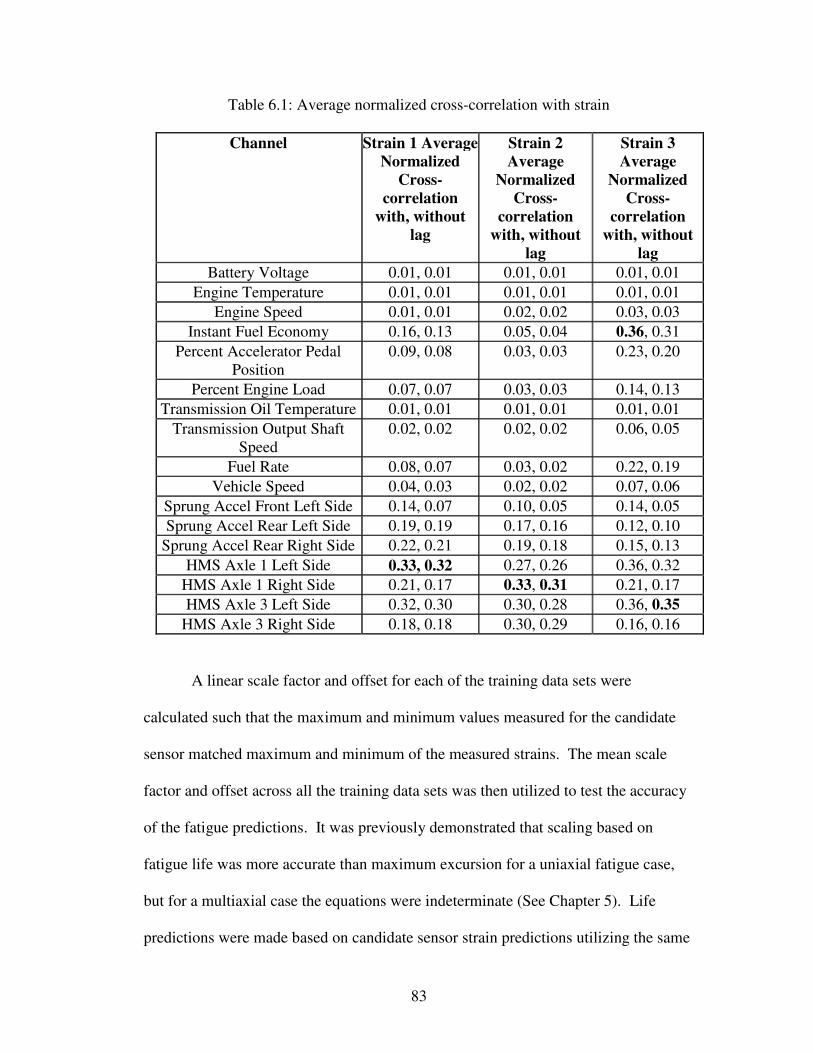
83

Table 6.1: Average normalized cross-correlation with strain

Channel Strain 1 Average

Normalized

Cross-

correlation

with, without

lag

Strain 2

Average

Normalized

Cross-

correlation

with, without

lag

Strain 3

Average

Normalized

Cross-

correlation

with, without

lag

Battery Voltage 0.01, 0.01 0.01, 0.01 0.01, 0.01

Engine Temperature 0.01, 0.01 0.01, 0.01 0.01, 0.01

Engine Speed 0.01, 0.01 0.02, 0.02 0.03, 0.03

Instant Fuel Economy 0.16, 0.13 0.05, 0.04 0.36, 0.31

Percent Accelerator Pedal

Position

0.09, 0.08 0.03, 0.03 0.23, 0.20

Percent Engine Load 0.07, 0.07 0.03, 0.03 0.14, 0.13

Transmission Oil Temperature 0.01, 0.01 0.01, 0.01 0.01, 0.01

Transmission Output Shaft

Speed

0.02, 0.02 0.02, 0.02 0.06, 0.05

Fuel Rate 0.08, 0.07 0.03, 0.02 0.22, 0.19

Vehicle Speed 0.04, 0.03 0.02, 0.02 0.07, 0.06

Sprung Accel Front Left Side 0.14, 0.07 0.10, 0.05 0.14, 0.05

Sprung Accel Rear Left Side 0.19, 0.19 0.17, 0.16 0.12, 0.10

Sprung Accel Rear Right Side 0.22, 0.21 0.19, 0.18 0.15, 0.13

HMS Axle 1 Left Side 0.33, 0.32 0.27, 0.26 0.36, 0.32

HMS Axle 1 Right Side 0.21, 0.17 0.33, 0.31 0.21, 0.17

HMS Axle 3 Left Side 0.32, 0.30 0.30, 0.28 0.36, 0.35

HMS Axle 3 Right Side 0.18, 0.18 0.30, 0.29 0.16, 0.16

A linear scale factor and offset for each of the training data sets were

calculated such that the maximum and minimum values measured for the candidate

sensor matched maximum and minimum of the measured strains. The mean scale

factor and offset across all the training data sets was then utilized to test the accuracy

of the fatigue predictions. It was previously demonstrated that scaling based on

fatigue life was more accurate than maximum excursion for a uniaxial fatigue case,

but for a multiaxial case the equations were indeterminate (See Chapter 5). Life

predictions were made based on candidate sensor strain predictions utilizing the same

84

fatigue analysis software and equations used in the high fidelity fatigue estimates.

Results from the training data sets were labeled 1-5 and the testing data sets were

labeled A-D for the scaled candidate sensors. Values were plotted and compared to

the high fidelity fatigue model results in Figure 6.2.

1 2 3 4 5 A B C D10

0

102

104

106

108

Life Predictions

Life (

mile

s)

Course

Strain Based

CC w/o Lag Candidate

CC w/ Lag Candidate

Figure 6.2: Life estimate using Cross-Correlation (CC)

6.3.2 Coefficient of Determination of Root Mean Square

A comparison of Root Mean Square or RMS values for linearity was used

previously to determine if relative magnitude of individual time segments are

proportional [20]. Relative magnitude of strain cycles are essential to calculating

fatigue, so a process was developed to evaluate the linearity of the comparison. Strain

and predictor channels were separated into five second blocks. RMS, denoted as z in

equation 2 below, was calculated for each time sample of the strain or predictor

channel (xi) in the block.

Training Courses Testing Courses

85

∑=

=n

i

ixn

z1

21 (2)

The coefficient of determination (R2) was then calculated based on the RMS values

(z), a least squares, linear fit of the sensor RMS blocks to the strain RMS blocks ( z )

and the average sensor value ( z ).

∑

∑

−

−

−=

i

i

i

ii

zz

zz

R2

2

2

)(

)ˆ(

1 (3)

Resulting coefficient of determination values for each sensor are listed in Table 6.2

with the maximum values in bold font.

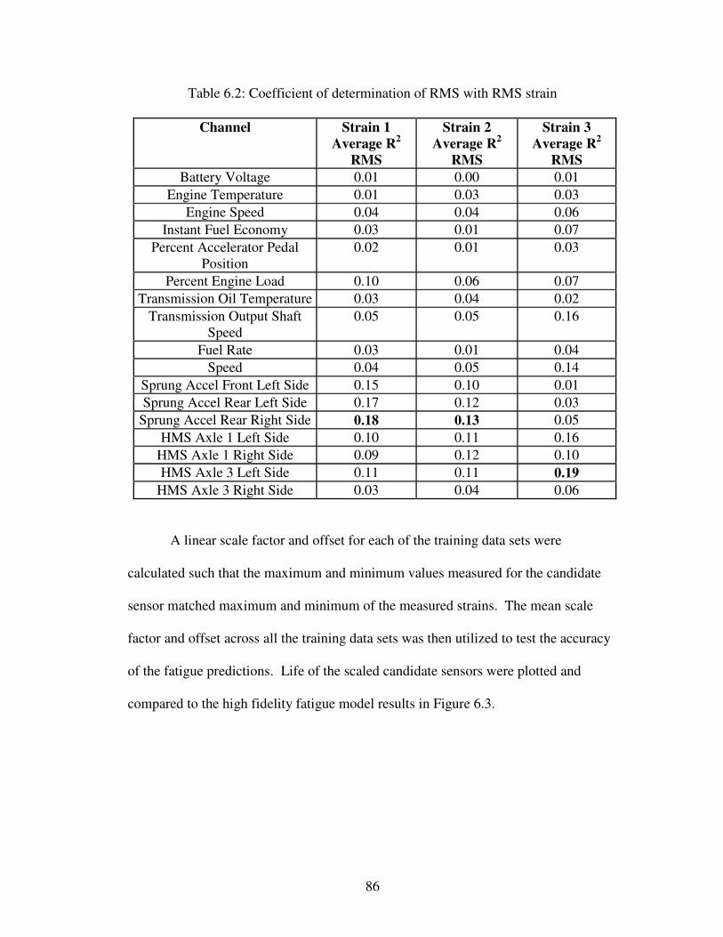
86

Table 6.2: Coefficient of determination of RMS with RMS strain

Channel Strain 1

Average R2

RMS

Strain 2

Average R2

RMS

Strain 3

Average R2

RMS

Battery Voltage 0.01 0.00 0.01

Engine Temperature 0.01 0.03 0.03

Engine Speed 0.04 0.04 0.06

Instant Fuel Economy 0.03 0.01 0.07

Percent Accelerator Pedal

Position

0.02 0.01 0.03

Percent Engine Load 0.10 0.06 0.07

Transmission Oil Temperature 0.03 0.04 0.02

Transmission Output Shaft

Speed

0.05 0.05 0.16

Fuel Rate 0.03 0.01 0.04

Speed 0.04 0.05 0.14

Sprung Accel Front Left Side 0.15 0.10 0.01

Sprung Accel Rear Left Side 0.17 0.12 0.03

Sprung Accel Rear Right Side 0.18 0.13 0.05

HMS Axle 1 Left Side 0.10 0.11 0.16

HMS Axle 1 Right Side 0.09 0.12 0.10

HMS Axle 3 Left Side 0.11 0.11 0.19

HMS Axle 3 Right Side 0.03 0.04 0.06

A linear scale factor and offset for each of the training data sets were

calculated such that the maximum and minimum values measured for the candidate

sensor matched maximum and minimum of the measured strains. The mean scale

factor and offset across all the training data sets was then utilized to test the accuracy

of the fatigue predictions. Life of the scaled candidate sensors were plotted and

compared to the high fidelity fatigue model results in Figure 6.3.

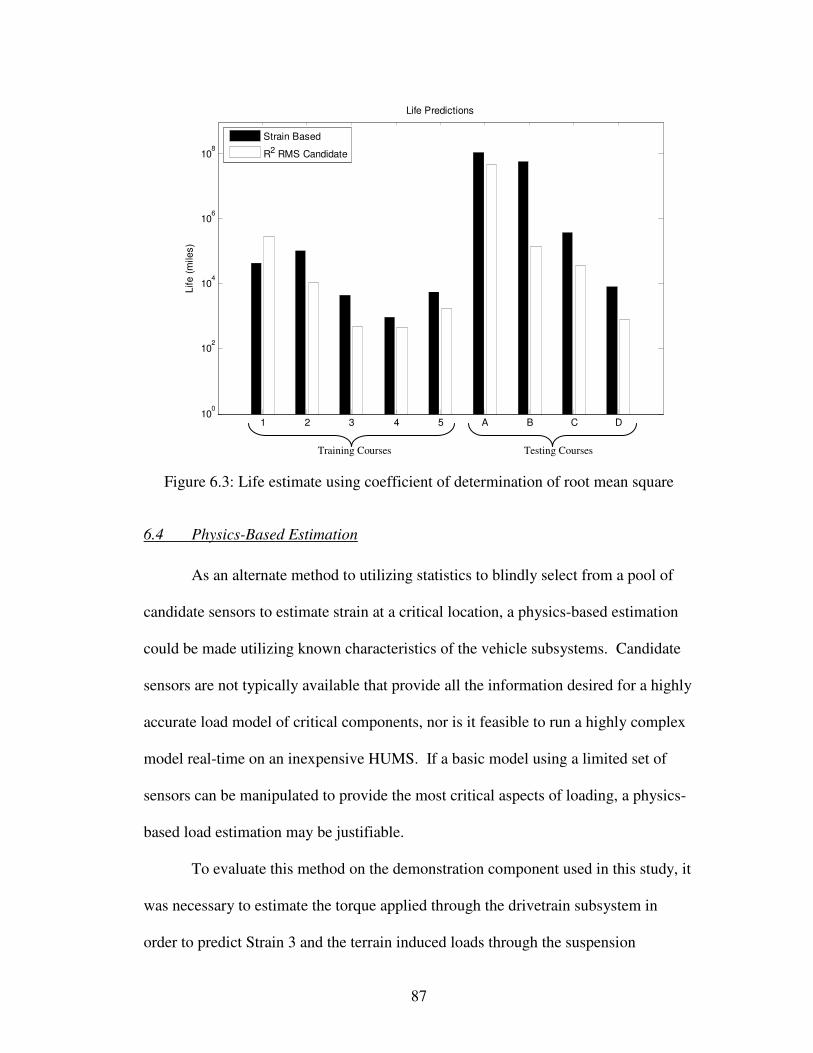
87

1 2 3 4 5 A B C D10

0

102

104

106

108

Life Predictions

Life (

mile

s)

Course

Strain Based

R2 RMS Candidate

Figure 6.3: Life estimate using coefficient of determination of root mean square

6.4 Physics-Based Estimation

As an alternate method to utilizing statistics to blindly select from a pool of

candidate sensors to estimate strain at a critical location, a physics-based estimation

could be made utilizing known characteristics of the vehicle subsystems. Candidate

sensors are not typically available that provide all the information desired for a highly

accurate load model of critical components, nor is it feasible to run a highly complex

model real-time on an inexpensive HUMS. If a basic model using a limited set of

sensors can be manipulated to provide the most critical aspects of loading, a physics-

based load estimation may be justifiable.

To evaluate this method on the demonstration component used in this study, it

was necessary to estimate the torque applied through the drivetrain subsystem in

order to predict Strain 3 and the terrain induced loads through the suspension

Training Courses Testing Courses

88

subsystem to predict Strain 1 and Strain 2. A simplified drivetrain model was

developed which utilized engine speed, vehicle speed and a simplified shift map to

estimate engine load inputs. Transmission output shaft speeds, component

geometries, and material properties were used to estimate the resulting reaction

torques and convert load information to strain at the critical area. A simple

suspension model was developed based on sprung and unsprung masses, sprung mass

acceleration near the example component and unsprung mass acceleration via

differentiated HMS reading. Strain predictions were implemented into the multiaxial

fatigue model and compared to the high-fidelity fatigue predictions. Physics-based

predictions were shown to be significantly less accurate for the example component

than the estimates made based on the blind sensor selection. This may be attributable

to the simplifications necessary to make the physics-based models run in real-time,

the limited set of sensors, the locations from which the subsystem load predictions

were made or the fidelity of the sensor data.

6.5 Hybrid Models

To investigate the poor quality of the physics-based predictions, the average

normalized cross-correlation and coefficient of determination of root mean square

statistics were calculated for the physics-based strain predictions to determine which

subsystem model resulted in the significantly less accurate fatigue predictions. In

general, the loading seen in Strain 1 and Strain 2 were attributed to the terrain induced

loading through the suspension subsystem and Strain 3 was attributed to the

drivetrain. Results are shown in Table 6.3.

89

Table 6.3: Physics-based comparison

Estimator Strain 1

Average

Strain 2

Average

Strain 3

Average

Average Normalized Cross-

Correlation with Lag

0.03 0.03 0.15

Average Normalized Cross-

Correlation without Lag

0.03 0.03 0.14

R2 RMS 0.14 0.10 0.07

Average normalized cross-correlation statistics suggest that the powertrain

subsystem model was the cause of the poor predictions, while the coefficient of

determination of root mean squares suggests the suspension model was the issue.

Two hybrid models were developed. Hybrid Model A utilized the physics-based

suspension model to predict strains 1 and 2. Strain 3 was predicted based on the

average normalized cross-correlation statistic without a time lag candidate sensor.

Hybrid model B utilized the physics-based powertrain model to predict strain 3 and

the average normalized cross-correlation without lag statistic candidate for strains 1

and 2. Both models showed improvement over the physics-based strain estimation

model, but the Hybrid B model gave the most accurate fatigue predictions. Life

predictions based on the Hybrid B model were plotted and compared to the high

fidelity fatigue model results in Figure 6.4.

90

1 2 3 4 5 A B C D10

0

102

104

106

108

Life Predictions

Life (

mile

s)

Course

Strain Based

Hybrid B Candidate

Figure 6.4: Life estimate using Hybrid B model

6.6 Results

As would be expected the life estimated on the training courses and shown in

Figures 6.2, 6.3, and 6.4 were fairly accurate. In order to compare the accuracy of

various models on the testing courses, a representative usage made up of the available

terrain types was necessary. Requirements documents indicate a predicted usage in

terms of primary, secondary and off-road courses for each variant of the

demonstration vehicle. Durability tests for army combat vehicles are commonly

20,000 miles in length. Predictions of the fatigue damage accumulated over a 20,000

mile test following the expected terrain profile for the most common variant were

made based on the testing data sets A-D for each model. Results are listed in Table

6.4. As a point of comparison, the most accurate terrain identification models

Training Courses Testing Courses

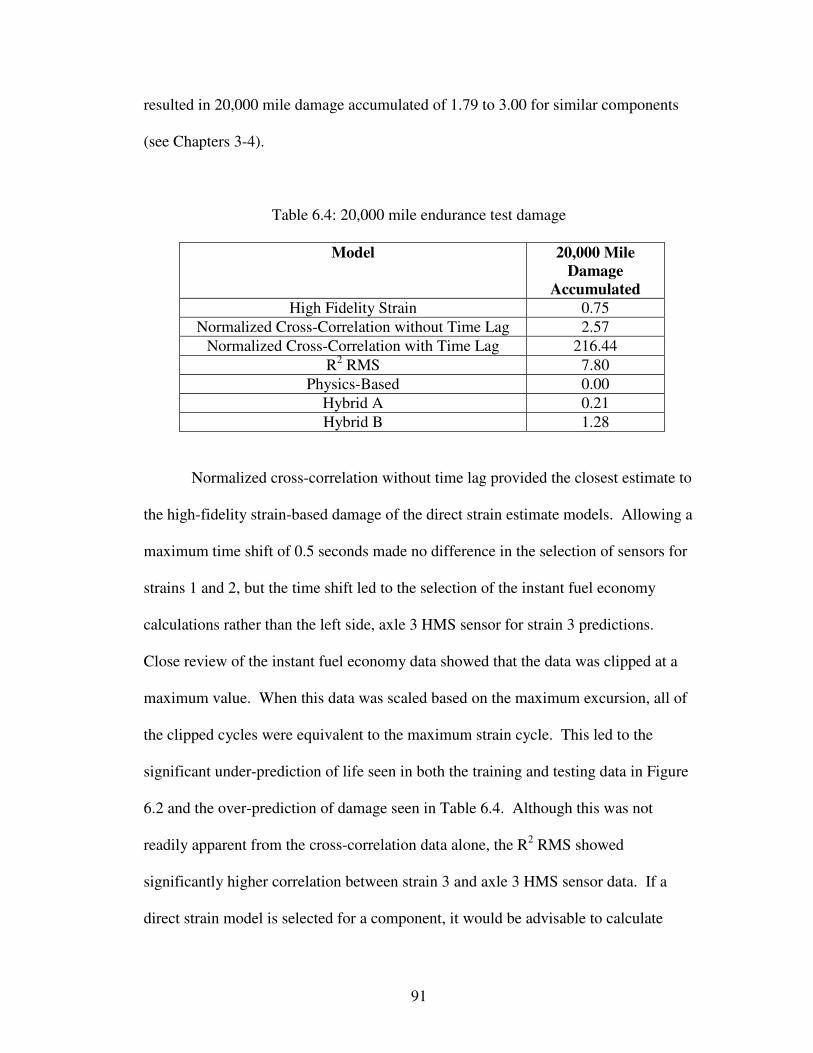
91

resulted in 20,000 mile damage accumulated of 1.79 to 3.00 for similar components

(see Chapters 3-4).

Table 6.4: 20,000 mile endurance test damage

Model 20,000 Mile

Damage

Accumulated

High Fidelity Strain 0.75

Normalized Cross-Correlation without Time Lag 2.57

Normalized Cross-Correlation with Time Lag 216.44

R2 RMS 7.80

Physics-Based 0.00

Hybrid A 0.21

Hybrid B 1.28

Normalized cross-correlation without time lag provided the closest estimate to

the high-fidelity strain-based damage of the direct strain estimate models. Allowing a

maximum time shift of 0.5 seconds made no difference in the selection of sensors for

strains 1 and 2, but the time shift led to the selection of the instant fuel economy

calculations rather than the left side, axle 3 HMS sensor for strain 3 predictions.

Close review of the instant fuel economy data showed that the data was clipped at a

maximum value. When this data was scaled based on the maximum excursion, all of

the clipped cycles were equivalent to the maximum strain cycle. This led to the

significant under-prediction of life seen in both the training and testing data in Figure

6.2 and the over-prediction of damage seen in Table 6.4. Although this was not

readily apparent from the cross-correlation data alone, the R2 RMS showed

significantly higher correlation between strain 3 and axle 3 HMS sensor data. If a

direct strain model is selected for a component, it would be advisable to calculate

92

both statistics in order to select the most appropriate candidate sensors. An alternate

method of determining the scaling and offset based on fatigue rather than the

maximum excursion may also improve fatigue predictions for the direct strain

models.

The physics-based model developed required significantly more

computational power and had poor predictive capabilities due to the limited ability of

the suspension model developed to predict strains 1 and 2. When the normalized

cross-correlation without time lag model for predicting strains 1 and 2 was combined

with the powertrain model for predicting strain 3 in the Hybrid B model, the damage

estimate over the 20,000 mile endurance test was much improved. This demonstrates

that the use of a physics-based model can improve fatigue damage predictions if the

component monitored justifies the additional computational load. Failure of the

suspension model is attributed to the lack of quality sensor data at the critical

locations necessary to make a high fidelity strain prediction. Sensor data may not be

of the quality required to make accurate predictions in current vehicles, but inclusion

of higher quality sensors at critical locations may be justifiable for future vehicles

designed for use with HUMS and remaining life prognostics.

6.7 Conclusions

In order to utilize HUMS and remaining life prognostics to obtain the desired

improvements in reliability and availability on military ground vehicles within a

reasonable cost, durable sensors that provide loading information for fatigue sensitive

components are critical. Strain is often the desired input for fatigue calculations, but

most common sensors used to measure strain including adhesively bonded electric

93

resistant wire strain gauges, are neither rugged nor reliable enough for a military

ground vehicle environment. In addition, the sensors need to provide data for many

of the components on a vehicle. Components susceptible to fatigue damage that

should be monitored using a HUMS are not clearly recognized during the design of a

vehicle system, so sensors that indicate loading to a wide variety of components are

preferred. Use of sensors already integrated within the vehicle is an ideal source from

which to estimate strain due to their high reliability and minimal additional cost.

Add-on sensors such as accelerometers and GPS units are robust, easy to apply and

make a good alternate source for strain estimates. For many modern military

vehicles, the combination of integrated and add-on sensors make a large group of

candidates available for use in a HUMS, but the best indicators of strain may not be

clearly identifiable. A method is needed to identify and select sensors that provide

inputs suitable for fatigue damage models.

Two statistics were evaluated based on ability to identify data that provides

accurate fatigue predictions for a complexly loaded component on a military wheeled

vehicle. Normalized cross-correlation without time lag provided the most accurate

fatigue estimate of the direct strain calculations. Allowing for time shift was shown

to have a minor effect on the ranking of candidate components, but calculation of the

coefficient of determination of root mean square statistics as an additional means of

comparison are recommended for identifying the best candidate sensor.

As an alternate method to utilizing statistics to select sensors that indicate

strain on a component, a physics-based estimation can be made from the sensor data

available and known characteristics of the vehicle subsystems. More complex

94

physics-based subsystem loading models and geometry data were shown to improve

the fidelity of fatigue predictions, but quality sensor data at critical locations is

essential. Generally an improvement in the accuracy of fatigue predictions was

demonstrated as the HUMS and remaining life prognostics algorithms increase in

complexity. Selection of the model to be used on a specific component requires a

balance of the accuracy needed with the developmental and computational cost.

95

Chapter 7: Discussions and Summary

The goal of this research was to demonstrate that HUMS and remaining life

prognostics are feasible for military wheeled vehicles and develop methods to assist

in their application. Wheeled vehicles have many characteristics which make

application of HUMS a challenge. Foremost among these are the large number of

unique components that have complex loading profiles and are relatively inexpensive.

Methods for application and appropriate algorithms are necessary to enable a balance

of accuracy of the remaining life estimates with development complexity,

computational power required and cost.

Incorporating HUMS into a military vehicle life cycle is also a worthy goal.

Military ground vehicles typically go through a series of distinct phases during

development, testing, operation and disposal that are marked by key milestones and

tests. Incorporating HUMS architecture with the military vehicle life cycle would

allow designers to take advantage of required phases and tests to tune models and

minimize any detriments to the cost or schedule caused by HUMS implementation.

Methods and algorithms that are designed to take advantage of the military life cycle

would increase the likelihood of a successful HUMS.

This research was successful in demonstrating that HUMS are a viable

technology for improving the reliability and availability of military wheeled vehicles.

Fatigue of metal components is a common failure mode on military vehicles, and

failures of this type have a major effect on vehicle reliability and availability.

Algorithms specific to predicting damage accumulated through metal fatigue were

96

developed that could be reasonably computed real-time as part of an on-board,

inexpensive HUMS. Methods for identifying critical data and instrumentation were

also described. The methods and algorithms were demonstrated for a variety of

components on a military wheeled vehicle, and validation was performed by

comparing the results of the remaining life prognostics with those from high fidelity

physics of failure models.

7.1 Model Fidelity

To apply a HUMS to relatively inexpensive equipment such as military

wheeled vehicles, reasonable limitations must be applied to the hardware to minimize

cost. Resources for computation and processing must be used economically. For a

HUMS with limited computational resources, model fidelity and complexity are

critical issues. The case studies developed in Chapters 3 through Chapter 6 showed

that accuracy is roughly correlated with model complexity. Generally, as the

computational power that a fatigue damage model requires increases, the estimates of

damage accumulated become more accurate. The simplest computational models

were discussed in Chapters 3 and 4. These models utilized a feature recognition

technique to identify terrain or usage conditions and assign damage for time exposed.

A single set of algorithms based on a simple statistic provides monitoring for all the

components subjected to a particular loading condition. Additional scale factors

would attribute the load appropriately to other components and allow damage

accumulation to be calculated for these components with little increase in

computational complexity.

97

More computationally intensive models that predict strain at a critical location

from robust sensor data were introduced in Chapters 5 and 6. Predicted strain is used

to calculate fatigue damage accumulated through rainflow cycle counting, Basquin’s

equation, and Miner’s damage summation rule. These algorithms require more

computational power, but are simple enough to be used real-time. Results are limited

to a single failure mode of a single component. Removal of cycles based on

amplitude and frequency were evaluated based on ability to enhance prediction

capability in Chapter 5, but these techniques required additional computations and

showed little improvement in fatigue damage prediction.

The highest fidelity models were demonstrated in Chapter 6 and utilized

detailed physics-based subsystem models or a combination of physics-based and

direct strain models that would account for the individual loads applied to a

component. Subsystem models were used to calculate the dynamic loading for a

component, and mechanics of materials were used to predict strain at the critical

location for each time step. Similar methods to those used in the direct strain models

were leveraged to calculate damage accumulated and life remaining. The vehicle

subsystem models developed may be able to provide loading information to other

components being monitored, but they also require many inputs in order to provide

accurate loading conditions. Mechanics of materials models also can be

computationally intensive to convert the loads to strain at the critical area. These

models are geometry and failure mode specific, so each component monitored would

require a unique mechanics of materials model. For the example component in

Chapter 6, the subsystem and mechanics of materials models required significant

98

computational resources. Only a limited number of components could be modeled

with this degree of fidelity on a reasonably priced HUMS.

As potential components on a vehicle that could be monitored by HUMS are

discovered, it will become necessary to evaluate tradeoffs between cost of the HUMS,

level of fidelity, and number of components monitored. A number of elements must

be known to determine which models provide optimal returns on total vehicle

reliability and availability.

From a vehicle standpoint there are limited resources from which to perform

damage calculations. The number of components that will be monitored, the failure

modes of the monitored components, and the resources available are key inputs for

optimizing the HUMS and selecting damage models. Most vehicles have some

limited computational power for onboard systems currently, and vehicles that are

integrated with HUMS would likely have additional processing available or could be

expanded to have additional capability. The cost for adding computational power and

any limits imposed by size, electromagnetic interference, thermal load, and weight are

critical for optimizing HUMS results and selecting the most appropriate models for a

component. Representative estimates of usage are needed to calculate the return from

a HUMS model. In Chapters 4, 5 and 7, estimated usage from requirements

documents was used to evaluate model accuracy based on a realistic usage profile.

As HUMS are implemented on vehicles, data collected can be used to make

statistically significant estimations of the likely usage of vehicles rather than

approximations based on requirements documents.

99

Information specific to the failure mode and component is also critical to

determining the optimal models. In order to select the appropriate HUMS model for

a particular component failure, several component specific items need to be

investigated. Criticality of the failure is important because highly critical components

can have a detrimental effect on a large number of subsystems. If the component is

directly related to the safety of the operators, additional emphasis and accuracy may

be required for the prognostic model. A component that is particularly expensive or

whose failure leads to damage of expensive components may justify a higher level of

fidelity. Recovery and repair time in case of failure also affect component criticality.

Computational resources must be weighed and compared with the criticality of

components and the resources required to develop models in order to determine the

optimal HUMS solutions. Model fidelity for a particular component must be

determined by allocating resources based on criticality of the component, and the

effect on soldier safety, system reliability and system availability.

In order to determine the most appropriate model and level of fidelity to

utilize, a number of component, vehicle, and failure mode specific inputs need to be

weighed versus the HUMS properties. To achieve the best returns in terms of

reliability and availability improvements, potential accuracy of predictions needs to

be compared and representative estimates of usage determined in order to select the

most appropriate models.

7.2 Instrumentation and Sensors

Another key aspect for developing HUMS and remaining life prognostics is

selecting potential sensors that may be appropriate for the models and identifying

100

which sensors provide the inputs necessary to predict damage. In general, any

sensors used need to be reliable enough that the HUMS would not contribute

significantly to the total platform malfunctions. Frequent need for replacement or

calibration requiring human interaction would increase the logistics and maintenance

footprint of a vehicle and be counter to the goals of any HUMS. Physical or

analytical redundancy can improve the reliability and availability of instrumentation,

but redundancy needs to be balanced with the additional cost. Methods for selecting

the appropriate sensor data for damage models may also be required in cases where

appropriate indicators are not clearly identifiable.

7.2.1 Potential Sensors

A military ground vehicle provides a particularly difficult environment for

instrumentation and sensors. Military ground vehicles typically experience rough

terrain, extreme temperature changes, frequent exposure to dust and other

contaminants, and large fluctuations in humidity which are all detrimental to many

sensors. The focus of the models developed in this research is fatigue damage in

metals. This is a common mode of component failure for military wheeled vehicles.

Strain measurement is the typical input to fatigue damage models. The most common

method of measuring strain is through the use of adhesively bonded strain gauges, but

this is difficult because strain gauges are sensitive to environmental effects seen in a

military wheeled vehicle. Bonding can also be an issue if the gauges are expected to

last the life of the component. A review of the literature in Chapter 2 suggests that

novel sensing technologies such as Uni-Axial Strain Transducers (UAST),

piezoelectric sensors or even microelectromechanical systems may provide

101

significantly more reliable strain measurements to fatigue damage models. However,

significant development needs to be accomplished before these technologies will be

available. Instrumentation that is commonly obtainable and used frequently is more

likely to be inexpensive enough and ready for HUMS applications in military ground

vehicles.

The models developed in this research utilized sensors that were expected to

be sufficiently reliable for use in a HUMS applied to a military ground vehicle. The

sensors used can generally be split into two categories. The first are robust sensors

that are typically not as susceptible to environmental effects. The models developed

in Chapters 3 and 4 utilized speed via Global Positioning Satellite (GPS) sensors and

acceleration from accelerometers. Models developed in Chapters 5 and 6 also used

acceleration from accelerometers. GPS units are a well developed technology and

can provide additional useful data to vehicle operators. Many suppliers exist which

makes the technology less expensive. Hardened, durable versions are available and

can be easily adapted to a military vehicle. Accelerometers are also common sensors

that are used in a variety of testing environments. Accelerometers are relatively

durable and reasonable in cost which makes them a good candidate for use in a

HUMS.

The second category of sensors used to predict strain that is discussed in this

research is instrumentation designed-in during vehicle development. Models

developed in Chapter 6 utilized data from sensors already existing on the

demonstration vehicle. Most modern military vehicles are arrayed with a variety of

sensors to provide feedback to the driver, monitor specific parameters to identify

102

faults, or be used as a diagnostic tool when maintenance is performed. Use of sensors

already integrated within the vehicle is an ideal source from which to estimate input

parameters to a damage model. These sensors typically have high reliability due to

their use in other vehicle subsystems and the cost of integrating them within the

HUMS is minimal in comparison with the cost of adding an additional sensor.

Improvement in the quality of these sensors may be justified if the improvements

provide measurements more suitable for utilization in remaining life prognostics

algorithms. Sensors developed and integrated during the design phase of the vehicle

can be more cheaply implemented than those added after the design is finalized.

These sensors are more robust when they are added during design because the

surrounding structure can be manipulated to provide protection from adverse

environmental effects. Connections and communication links also have increased

durability and survivability when they are added during the design phase.

7.2.2 Strain Indicators

Another issue for sensors in HUMS applications is that the combination of

integrated and add-on sensors make a large group of candidates, but the best

indicators of strain may not be clearly identifiable. Two methods to identify and

select sensors that provide inputs suitable for fatigue damage models were proposed

in Chapter 6.

The first method utilized to identify strain indicators was the use of statistics

to show a relationship between the critical strain and potential sensors. Two statistics

were evaluated based on ability to identify data that provides accurate fatigue

predictions for a complexly loaded component on a military wheeled vehicle. Results

103

from the case study in Chapter 6 showed that normalized cross-correlation provides

the most accurate fatigue estimates, but calculation of the coefficient of determination

of root mean square statistics as an additional means of comparison is recommended

for identifying the best overall candidate sensor.

As an alternate method to utilizing statistics to select sensors that indicate

strain on a component, sensors can be selected based on those necessary to provide

input to a physics-based estimation of the loading on vehicle subsystems. A physics-

based estimation may require a large number of sensors, and the subsystem level

information required to implement the models may be significant. Results from the

case study in Chapter 6 showed that the quality of data provided by sensors is a key

contributor to the ability to make accurate damage estimations using physics-based

load models.

7.3 Summary and Contributions

In summary, this research was successful in demonstrating that HUMS are a

viable technology for tracking fatigue of metal components in military wheeled

vehicles. Algorithms specific to predicting damage accumulated were developed that

could be reasonably computed real-time as part of an on-board, inexpensive HUMS.

A range of models were developed and fidelity of the models was shown to be

correlated with the computational complexity. Simplistic models that tracked a large

number of components had the least potential for accurate fatigue damage predictions

while high fidelity physics-based models had the most potential. Recommendations

for the information needed to select the most appropriate model for a component and

optimize the effect on vehicle reliability and availability were made. Methods for

104

identifying the set of instrumentation that could reasonably be used as part of a

HUMS, and techniques for selecting the instrumentation that provides inputs for

metal fatigue damage models were evaluated. Example vehicles and components

were selected and results were compared with high fidelity physics of failure models

to demonstrate feasibility of the developed algorithms (See Appendix A).

Recommendations and reasoning were made for incorporation of HUMS

development throughout a military vehicle life cycle.

The processes developed could be easily adapted to other platforms including

commercial fleets of vehicles or aircraft. The algorithms and techniques evaluated

provide potential for improving reliability and availability, but it should be noted that

other methods may be more appropriate depending on the specific vehicle and failure

mode. Fixed interval replacement, sparing or component redesign may be more

suitable depending on the mode of failure, criticality of component, and HUMS costs.

7.4 Limitations and Future Work

In general significant work remains before there can be widespread

application of HUMS and remaining life prognostics on military ground vehicles.

The only failure mode investigated in this research was fatigue on metals. Other

materials and modes of failure would need to be similarly evaluated to determine if

HUMS and remaining life prognostics can be performed for a military wheeled

vehicle.

Each of the models developed in this work were based on a single vehicle and

operator on courses within a limited geographic area. Vehicle setup and usage can

vary significantly and the effects of these changes were not quantified in this analysis.

105

Changes based on locataion and weather also were not considered. Courses that

represent the full spectrum of terrain types likely to be encountered should be

evaluated and the variations between operators and vehicles should be analyzed

before the proposed HUMS models are universally applied.

From a systems level standpoint, guidelines or methods for evaluating the

improvements of reliability and availability due to HUMS technology versus other

options are needed. Gains in vehicle reliability and availability need to be weighed

against the cost, time to develop and repair time of a system to determine what

method is most appropriate. It is unlikely that all the information will be known to

optimize the number of components modeled and type of models used, so guidelines

or estimating techniques are needed to provide a reasonable balance of resources with

needs. New metrics are needed for estimating effects of HUMS on reliability growth

models and system evaluations.

Recommendations for selecting sensors to provide reliable inputs to remaining

life prognostics models were discussed. However, no sensing technology can

guarantee perfect reliability. Methods for error checking are needed to provide

warning of sensor failure and prevent premature replacement of the monitored

component or missed damage cycles. Techniques and algorithms are needed to deal

with signal interruption or contamination. If redundant sensors are used, methods to

determine which sensor provides the most accurate data are needed.

Specific to the models developed here, there are also a number of limitations

that need to be addressed. A more thorough investigation of the frequency content

may indicate the critical aspects of loading and minimize the number of cycles that

106

are necessary to analyze. Relationships between critical frequencies and terrain type,

input sensors, or even vehicle speed may improve accuracy of the remaining life

prognostics models developed in Chapters 3 through 6 while decreasing the required

computational effort.

For the terrain sensing models described in Chapters 3 and 4, limits were

developed based on a single vehicle. Variations between vehicles and drivers would

need to be quantified and addressed for these algorithms to be applied to a fleet. The

models in Chapters 3 and 4 utilized an accelerometer on the sprung mass of the

vehicle as the input to terrain identification algorithms. An accelerometer on the

unsprung mass may provide more consistent readings between vehicles regardless of

condition or payload.

A method to identify components analytically where acceleration and strain

have similar waveforms would be useful to determine when models such as the direct

strain model in Chapter 5 are applicable. The method proposed required collection of

test data to determine if measured acceleration and strain were suitably compatible.

Analytical models may help to identify the instrumentation and location necessary to

obtain the strain proportional waveforms required by the direct strain models in

Chapters 5 and 6.

For the direct strain models discussed in Chapters 5 and 6, a nonlinear scaling

method may provide more accurate strain estimates and resulting fatigue damage

calculations. Linear scaling was used to maintain a simple relationship between input

channels and strain, but a power or exponential function may provide more accurate

results with minimal increase in computational effort. The scaling method used in

107

Chapter 6 for multiaxial strain was based on absolute maximums. The studies on the

uniaxial case in Chapter 5 showed that fatigue based scaling provided significantly

more accurate damage predictions. A method to implement fatigue based scaling

could improve HUMS predictions on a multiaxial case similarly.

The research proposed a methodology for implementing HUMS and

remaining life prognostics on military wheeled vehicles. While the algorithms

developed are limited to metal fatigue, many of the constraints and requirements

should be applicable to a broad range of failure mechanisms. Significant work

remains to implement these technologies, but increased reliability and availability of

military vehicle systems is a worthy goal.

108

Appendix A

A baseline physics of failure analysis was performed on the example

mechanical component and used to demonstrate that the proposed HUMS algorithms

are appropriate and provide suitably accurate fatigue predictions. Figure A.1

illustrates process for high fidelity physics of failure analyses used for mechanically

loaded components where metal fatigue has been identified as the root cause of

failure. Loading or strain data is collected from dynamics models or live testing at or

near the failure location of a component. Finite element analysis is used to map the

strain or loads to the strain at the critical location. A critical plane method or rainflow

cycle counting is then performed on the resulting strain time histories and the

equivalent damage is calculated for each cycle. The fatigue damage accumulation is

estimated based on a damage summation method.

Figure A.1: Physics of Failure process

Strain Time HistoryLive Data

Damage Cycles CountRainflow Cycles Count Life Prediction

DADS/Virtual Lab

Loads,

Accelerations

Finite Element Analysis

Strain Time HistoryLive Data Strain Time HistoryLive Data

Damage Cycles CountRainflow Cycles Count Life PredictionDamage Cycles CountRainflow Cycles Count Life Prediction

DADS/Virtual LabDADS/Virtual Lab

Loads,

Accelerations

Finite Element Analysis

109

Appendix B

Normalized cross-correlation and coefficient of determination of RMS were

evaluated based on ability to identify data that provide accurate fatigue predictions.

To investigate the consistency of indicators between terrain types, results for the

training data were separated into primary, secondary and off-road terrains. Results

from the normalized cross-correlation, with and without a maximum time shift of 0.5

seconds, are listed in Table B.1 through B.3. Coefficient of determination of RMS

results are listed in Table B.4 through B.6. The candidate sensor with maximum

values of average normalized cross correlation for the strains attributed to terrain

induced loading (Strain 1 and Strain 2) and the drivetrain torque (Strain 3) are labeled

in bold font.

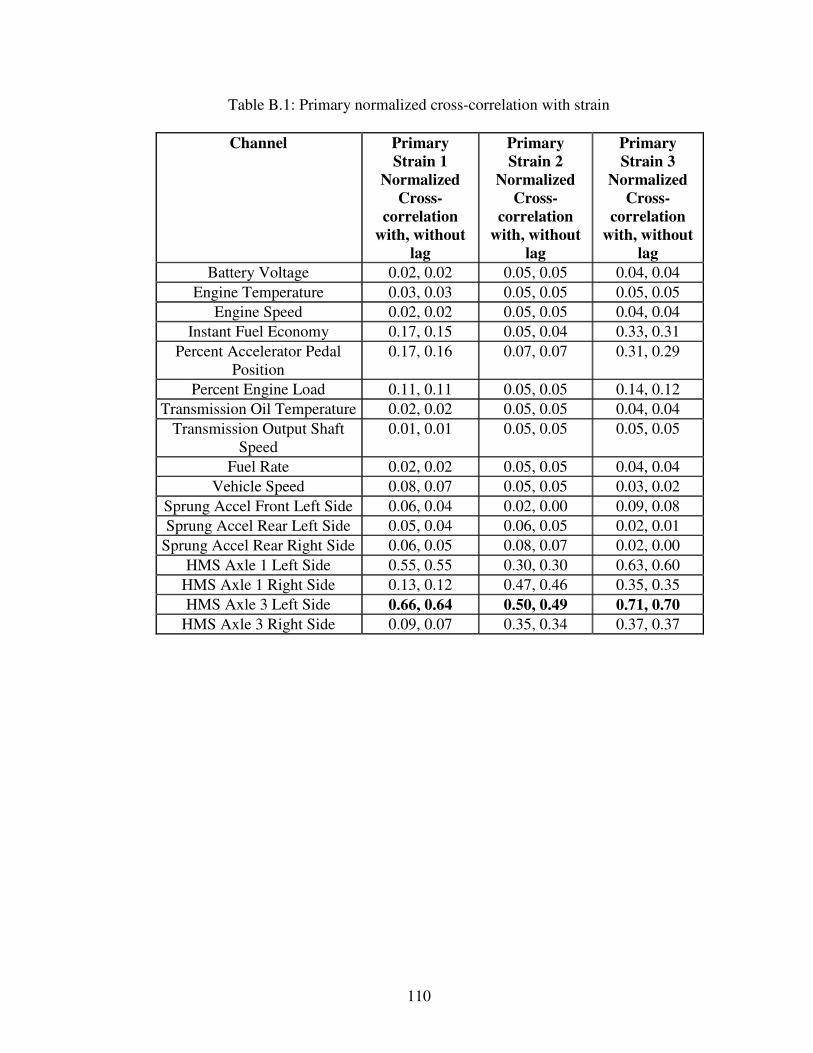
110

Table B.1: Primary normalized cross-correlation with strain

Channel Primary

Strain 1

Normalized

Cross-

correlation

with, without

lag

Primary

Strain 2

Normalized

Cross-

correlation

with, without

lag

Primary

Strain 3

Normalized

Cross-

correlation

with, without

lag

Battery Voltage 0.02, 0.02 0.05, 0.05 0.04, 0.04

Engine Temperature 0.03, 0.03 0.05, 0.05 0.05, 0.05

Engine Speed 0.02, 0.02 0.05, 0.05 0.04, 0.04

Instant Fuel Economy 0.17, 0.15 0.05, 0.04 0.33, 0.31

Percent Accelerator Pedal

Position

0.17, 0.16 0.07, 0.07 0.31, 0.29

Percent Engine Load 0.11, 0.11 0.05, 0.05 0.14, 0.12

Transmission Oil Temperature 0.02, 0.02 0.05, 0.05 0.04, 0.04

Transmission Output Shaft

Speed

0.01, 0.01 0.05, 0.05 0.05, 0.05

Fuel Rate 0.02, 0.02 0.05, 0.05 0.04, 0.04

Vehicle Speed 0.08, 0.07 0.05, 0.05 0.03, 0.02

Sprung Accel Front Left Side 0.06, 0.04 0.02, 0.00 0.09, 0.08

Sprung Accel Rear Left Side 0.05, 0.04 0.06, 0.05 0.02, 0.01

Sprung Accel Rear Right Side 0.06, 0.05 0.08, 0.07 0.02, 0.00

HMS Axle 1 Left Side 0.55, 0.55 0.30, 0.30 0.63, 0.60

HMS Axle 1 Right Side 0.13, 0.12 0.47, 0.46 0.35, 0.35

HMS Axle 3 Left Side 0.66, 0.64 0.50, 0.49 0.71, 0.70

HMS Axle 3 Right Side 0.09, 0.07 0.35, 0.34 0.37, 0.37

111

Table B.2: Secondary normalized cross-correlation with strain

Channel Secondary

Strain 1

Normalized

Cross-

correlation

with, without

lag

Secondary

Strain 2

Normalized

Cross-

correlation

with, without

lag

Secondary

Strain 3

Normalized

Cross-

correlation

with, without

lag

Battery Voltage 0.01, 0.01 0.00, 0.00 0.00, 0.00

Engine Temperature 0.01, 0.01 0.00, 0.00 0.01, 0.01

Engine Speed 0.01, 0.01 0.02, 0.02 0.02, 0.02

Instant Fuel Economy 0.21, 0.16 0.06, 0.04 0.44, 0.40

Percent Accelerator Pedal

Position

0.09, 0.07 0.02, 0.01 0.29, 0.26

Percent Engine Load 0.10, 0.10 0.05, 0.04 0.22, 0.21

Transmission Oil Temperature 0.01, 0.01 0.00, 0.00 0.01, 0.01

Transmission Output Shaft

Speed

0.01, 0.01 0.01, 0.01 0.11, 0.10

Fuel Rate 0.14, 0.11 0.03, 0.01 0.35, 0.32

Vehicle Speed 0.02, 0.01 0.00, 0.00 0.11, 0.11

Sprung Accel Front Left Side 0.11, 0.01 0.09, 0.02 0.06, 0.01

Sprung Accel Rear Left Side 0.15, 0.14 0.15, 0.13 0.05, 0.01

Sprung Accel Rear Right Side 0.20, 0.18 0.19, 0.17 0.06, 0.03

HMS Axle 1 Left Side 0.23, 0.22 0.20, 0.20 0.33, 0.31

HMS Axle 1 Right Side 0.10, 0.09 0.19, 0.18 0.23, 0.22

HMS Axle 3 Left Side 0.36, 0.33 0.36, 0.34 0.41, 0.40

HMS Axle 3 Right Side 0.20, 0.20 0.31, 0.31 0.16, 0.16

112

Table B.3: Off road normalized cross-correlation with strain

Channel Off Road

Strain 1

Average

Normalized

Cross-

correlation

with, without

lag

Off Road

Strain 2

Average

Normalized

Cross-

correlation

with, without

lag

Off Road

Strain 3

Average

Normalized

Cross-

correlation

with, without

lag

Battery Voltage 0.00, 0.00 0.00, 0.00 0.00, 0.00

Engine Temperature 0.00, 0.00 0.00, 0.00 0.00, 0.00

Engine Speed 0.01, 0.01 0.01, 0.01 0.03, 0.03

Instant Fuel Economy 0.13, 0.11 0.04, 0.04 0.34, 0.29

Percent Accelerator Pedal

Position

0.06, 0.05 0.02, 0.02 0.18, 0.15

Percent Engine Load 0.04, 0.04 0.02, 0.01 0.11, 0.11

Transmission Oil Temperature 0.00, 0.00 0.00, 0.00 0.00, 0.00

Transmission Output Shaft

Speed

0.03, 0.03 0.01, 0.01 0.05, 0.04

Fuel Rate 0.08, 0.07 0.02, 0.02 0.23, 0.20

Vehicle Speed 0.03, 0.02 0.01, 0.01 0.07, 0.06

Sprung Accel Front Left Side 0.17, 0.10 0.13, 0.08 0.18, 0.06

Sprung Accel Rear Left Side 0.26, 0.26 0.22, 0.20 0.18, 0.17

Sprung Accel Rear Right Side 0.28, 0.27 0.23, 0.22 0.22, 0.21

HMS Axle 1 Left Side 0.29, 0.27 0.28, 0.26 0.28, 0.22

HMS Axle 1 Right Side 0.27, 0.22 0.34, 0.30 0.15, 0.09

HMS Axle 3 Left Side 0.19, 0.17 0.21, 0.19 0.23, 0.21

HMS Axle 3 Right Side 0.21, 0.20 0.28, 0.27 0.09, 0.09

For primary terrain, the height management system sensors provided very

accurate input for all three strains. The training course used for primary terrain

involved long straight portions followed by tight turns. The only significant

powertrain and suspension events would occur near the turns where the HMS was

also active. Thus, the measured strains would closely follow the HMS sensor located

near the component. The secondary and off road courses are significantly more

random and the behavior for both the powertrain and suspension subsystems are more

113

decoupled. Torque applied through the powertrain varies depending on upcoming

obstacles which leads to an engine parameter (instant fuel economy) providing the

best indication of powertrain induced torque. HMS sensors or sprung acceleration

still provide the best indication of suspension loading. Including delay made

relatively minor changes to the average cross-correlation values, although allowing

for a lag did result in the selection of a different input channel for Strain 3 on the

secondary and Strain 1 on the off road course.

Table B.4: Primary coefficient of determination of RMS with RMS strain

Channel Primary

Strain 1

R2 RMS

Primary

Strain 2

R2 RMS

Primary

Strain 3

R2 RMS

Battery Voltage 0.02 0.01 0.00

Engine Temperature 0.00 0.06 0.02

Engine Speed 0.00 0.01 0.04

Instant Fuel Economy 0.01 0.00 0.11

Percent Accelerator Pedal

Position

0.00 0.00 0.00

Percent Engine Load 0.01 0.03 0.01

Transmission Oil Temperature 0.00 0.03 0.01

Transmission Output Shaft

Speed

0.10 0.15 0.10

Fuel Rate 0.00 0.00 0.00

Speed 0.09 0.15 0.09

Sprung Accel Front Left Side 0.00 0.00 0.01

Sprung Accel Rear Left Side 0.02 0.03 0.01

Sprung Accel Rear Right Side 0.01 0.00 0.00

HMS Axle 1 Left Side 0.43 0.38 0.50

HMS Axle 1 Right Side 0.32 0.39 0.16

HMS Axle 3 Left Side 0.50 0.51 0.48

HMS Axle 3 Right Side 0.11 0.13 0.04

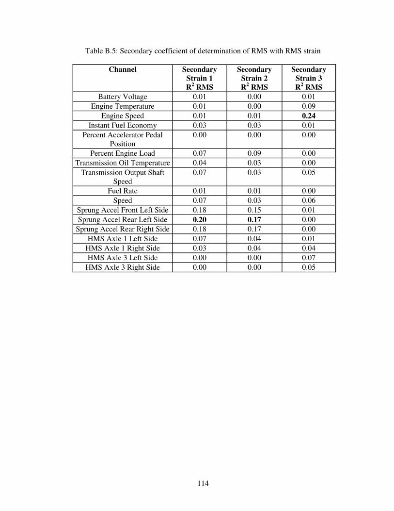
114

Table B.5: Secondary coefficient of determination of RMS with RMS strain

Channel Secondary

Strain 1

R2 RMS

Secondary

Strain 2

R2 RMS

Secondary

Strain 3

R2 RMS

Battery Voltage 0.01 0.00 0.01

Engine Temperature 0.01 0.00 0.09

Engine Speed 0.01 0.01 0.24

Instant Fuel Economy 0.03 0.03 0.01

Percent Accelerator Pedal

Position

0.00 0.00 0.00

Percent Engine Load 0.07 0.09 0.00

Transmission Oil Temperature 0.04 0.03 0.00

Transmission Output Shaft

Speed

0.07 0.03 0.05

Fuel Rate 0.01 0.01 0.00

Speed 0.07 0.03 0.06

Sprung Accel Front Left Side 0.18 0.15 0.01

Sprung Accel Rear Left Side 0.20 0.17 0.00

Sprung Accel Rear Right Side 0.18 0.17 0.00

HMS Axle 1 Left Side 0.07 0.04 0.01

HMS Axle 1 Right Side 0.03 0.04 0.04

HMS Axle 3 Left Side 0.00 0.00 0.07

HMS Axle 3 Right Side 0.00 0.00 0.05

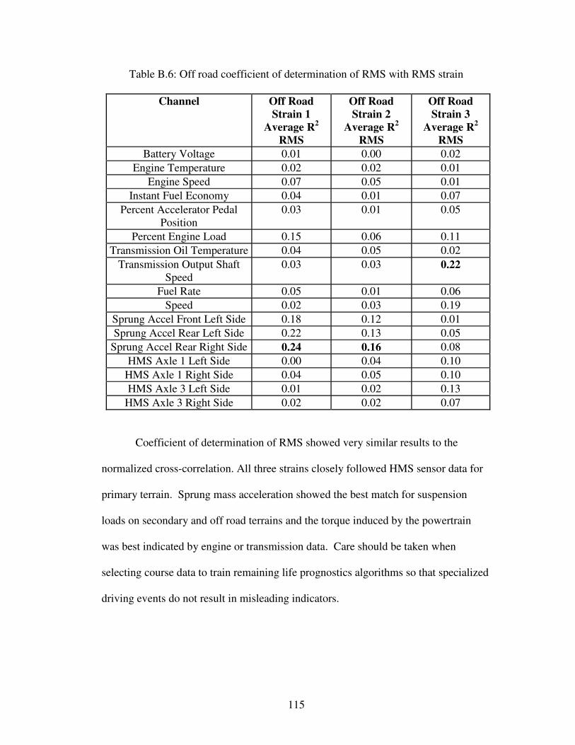
115

Table B.6: Off road coefficient of determination of RMS with RMS strain

Channel Off Road

Strain 1

Average R2

RMS

Off Road

Strain 2

Average R2

RMS

Off Road

Strain 3

Average R2

RMS

Battery Voltage 0.01 0.00 0.02

Engine Temperature 0.02 0.02 0.01

Engine Speed 0.07 0.05 0.01

Instant Fuel Economy 0.04 0.01 0.07

Percent Accelerator Pedal

Position

0.03 0.01 0.05

Percent Engine Load 0.15 0.06 0.11

Transmission Oil Temperature 0.04 0.05 0.02

Transmission Output Shaft

Speed

0.03 0.03 0.22

Fuel Rate 0.05 0.01 0.06

Speed 0.02 0.03 0.19

Sprung Accel Front Left Side 0.18 0.12 0.01

Sprung Accel Rear Left Side 0.22 0.13 0.05

Sprung Accel Rear Right Side 0.24 0.16 0.08

HMS Axle 1 Left Side 0.00 0.04 0.10

HMS Axle 1 Right Side 0.04 0.05 0.10

HMS Axle 3 Left Side 0.01 0.02 0.13

HMS Axle 3 Right Side 0.02 0.02 0.07

Coefficient of determination of RMS showed very similar results to the

normalized cross-correlation. All three strains closely followed HMS sensor data for

primary terrain. Sprung mass acceleration showed the best match for suspension

loads on secondary and off road terrains and the torque induced by the powertrain

was best indicated by engine or transmission data. Care should be taken when

selecting course data to train remaining life prognostics algorithms so that specialized

driving events do not result in misleading indicators.

116

Bibliography

Araiza, M. L., Kent, R., Espinosa, R. “Real-time, Embedded Diagnostics and

Prognostics in Advanced Artillery Systems.” AUTOTESTCON Proceedings

(2002): 818-841.

Barone, S., Ambrosio, P. D., Erto, P. “A Statistical Monitoring Approach for

Automotive On-board Diagnostic Systems.” Quality and Reliability

Engineering International 23 (2006): 565-575.

Bodden, D. S., Hadden, W., Grube, B. E., Clements, N. S. “Prognostics and Health

Management as Design Variable in Air-Vehicle Conceptual Design.” Journal

of Aircraft 43.4 (2006): 1053-1058.

Bechhoefer, E., Bernhard, A. “HUMS Optimal Weighting of Condition Indicators to

Determine the Health of a Component.” Annual Forum Proceeding –

American Helicopotor Society 1 (2004): 1186-1191.

Code of Practice for Fatigue Design and Assessment of Steel Structures. British

Standard BS 7608, 1993.

Ellerbrock, P. J., Halmos, Z., Shanthakumaran, P. “Development of New Health and

Usage Monitoring System Tools Using a NASA/Military Rotorcraft.” Annual

Forum Proceedings - American Helicopter Society 2 (1999): 2337-2348.

117

Engel, S. J., Gilmartin, B.J., Bongort, K, Hess, A. “Prognostics, The Real Issues

Involved with Predicting Life Remaining.” Proceedings of the 2000 IEEE

Aerospace Conference (2000): 457-469.

European Recommendations for Aluminum Alloy Structures Fatigue Design. Brussel:

ECCS – Technical Committee 2 Aluminum Alloy Structures, 1992.

Evans, A. “Flight Deck Indication of Health Monitoring Data - A Critique.”

Proceeding of the Institution of Mechanical Engineers Part G – Journal of

Aerospace Engineering 216.G5 (2002): 249-257.

Fackler, W. C. “A Review of Cumulative-Damage Theory,” Equivalence Techniques

for Vibration Testing.” The Shock and Vibration Information Center (1972):

5-32.

Fatemi, A., Socie, D. F. “A Critical Plane Approach to Multiaxial Fatigue Damage

Including Out-of-Phase Loading.” Fatigue and Fracture of Engineering

Materials and Structures 11.3 (1988): 149-165.

Gandhi, T., Chang, R., Trivedi, M. M. “Video and Seismic Sensor-Based Structural

Health Monitoring: Framework, Algorithms, and Implementation.” IEEE

Transactions on Intelligent Transportation Systems 8.2 (2007): 169-180.

118

Heine, R., Barker, D. “Simplified Terrain Identification and Component Fatigue

Damage Estimation Model For Use in a Health and Usage Monitoring

System.” Microelectronics Reliability doi:10.1016/j.microrel.2007.02.017

(2007).

Hunt, S. R., Hebden I.G. “Validation of the Eurofighter Typhoon Structural Health

and Usage Monitoring System.” Smart Materials & Structures 10.3 (2001):

497-503.

Fatemi, A., Socie, D. F. “A Critical Plane Approach to Multiaxial Fatigue Damage

Including Out-of-Phase Loading.” Fatigue and Fracture of Engineering

Materials and Structures 12 (1988): 149-165.

Gordon, A. C. “Development to Production of an Integrated Health and Usage

Monitoring System for Helicopters.” Aerospace Technology Conference and

Exposition SAE Technical Paper Series (1991): 1-31.

Greitzer, F. L., Pawlowski, R. A. “Embedded Prognostics Health Monitoring.”

Proceedings of the 48th

International Instrumentation Symposium 48 (2002):

301-310.

Hadden, S. C., Maurer, J. A. “Predicting Failure Using an On-Board Monitoring

System.” Time-Dependent Failure Mechanisms and Assessment

119

Methodologies - Proceedings of the 35th

Meeting of the Mechanical Failures

Prevention Group (1983): 229-236.

Jarrell, D. B., Bond, L. J. “Physics-Based Prognostics for Optimizing Plant

Operations.” Sound and Vibration 40.2 (2006): 12-15.

Kacprzynski, G. J., Roemer, M. J., Modgil, G., Palladino, A. “Enhancement of

Physics-of-Failure Prognostic Models with System Level Features.”

Proceedings of the IEEE Aerospace Conference 6 (2002): 2919-2925.

Krok, M. Goebel, K. “Prognostics for Advanced Compressor Health Monitoring.”

Proceedings of the SPIE 5107 (2003): 1-12.

Li, C. J., Ray, A. “Neural-Network Representation of Fatigue Damage Dynamics.”

Smart Materials & Structures 4.2 (1995): 126-133.

Martin, W., Collingwood, G., Barndt, G. “Structural Life Monitoring of the V-22.”

Annual Forum Proceedings – American Helicoptor Society 2 (1999): 2373-

2386.

Miner, M. A. “Cumulative Damage in Fatigue.” ASME Journal of Applied

Mechanics 12 (1945): 159-164.

120

Mourna, J. D., Steffen, V. “Impedance-based Health Monitoring for Aeronautic

Structures using Statistical Meta-modeling.” Journal of Intelligent Material

Systems and Structures 17 (2006): 1023-1036.

Ng, H. K., Chen, R. H., Speyer, J. L. “A Vehicle Health Monitoring System

Evaluated Experimentally on a Passenger Vehicle.” IEEE Transactions on

Control Systems Technology 14.5 (2006): 854-870.

Nothwang, W. D., Hirsch, S. G., Demaree, J. D., Hubbard, C. W.,Cole, M. W., Lin,

B., Giurgiutiu, V. “Direct Integration of Thin Film Piezoelectric Sensors with

Structural Materials for Structural Health Monitoring.” Integrated

Ferroelectrics 83 (2006): 139-148.

Pilkey, W. D. Formulas for Stress, Strain, and Structural Matrices. New York: John

Wiley and Sons, 1994.

“Prognostics and Health Management for the JSF Program.” Sound and Vibration

38.5 (2004): 8.

Ray, A., Tangirala, S. “Stochastic Modeling of Fatigue Crack Dynamics for On-line

Failure Prognostics.” IEEE Transactions on Control Systems Technology 4.4

(1996): 443-451.

121

Roemer, M. J., Kacprzynski, G. J., Schoeller, M. H. “Improved Diagnostic and

Prognostic Assessments Using Health Management Information Fusion.”

AUTOTESTCON Proceedings (2001): 365-377.

Schuster, E., Gross, K. C. “Multi-Frequency Sinusoidal Perturbation Method for

Dynamic Characterization of Multi-Processor Computer Servers.” Sun

Microsystems Laboratories Technical Report Series, SMLI TR-2004-130

(2004): 1-22.

Socie, D. F., Pompetzki, M. A. “Modeling Variability in Service Loading Spectra.”

ASTM Special Technical Publication 1450.JAI11561 (2004): 46-57.

Teal, R. S., Venuti, M. L., Heather, A. “Health and Usage Monitoring on the

International CH-47D.” Annual Forum Proceedings – American Helicopter

Society 3 (1997): 220-231.

Trammel, C., Vossler, G., Feldmann, M. “UK Ministry of Defense Generic Health

and Usage Monitoring System (GenHUMS).” Aircraft Engineering and

Aerospace Technology 69.5 (1997): 414+.

Veers, P. S., Winterstien, S. T., Nelson, D. B., Cornell, C. A. “Variable-Amplitude

Load Models for FatigueDamage and Crack Growth.” Development of

Fatigue Loading Spectra, ASTM STP 1006 (1989): 172-197.

122

Vichare, N. M., Pecht, M. G. “Prognostics and Health Management of Electronics.”

IEEE Transactions of Components and Packaging Technologies 29.1 (2006):

222-229.

Wakha, K., Majed, M. A., Dasgupta, A., Pines, D. J. “A Multi-Functional

Stress/Strain Sensor for Damage.” AIAA/ASME/ASCE/AHS/ASC Structures,

Structural Dynamics and Materials Conference 2 (2003): 1493-1503.

Wang, C. H., Brown, M. W. “A Path-Independent Parameter for Fatigue under

Proportional and Non-Proportional Loading.” Fatigue Fracture of Engineering

Materials and Structures 16 (1993): 1285-1298.

Wilson, J. R. “Prognostics May Save Engines – And Aircraft.” Aerospace America

35.7 (1997): 24-25.

Woodard, S. E., Coffey, N. C., Gonzalez, G. A. “Development and Flight Testing of

an Adaptable Vehicle Health-Monitoring Architecture.” Journal of Aircraft

41.3 (2004): 531-539.

Yan, J. H., Lee, J. “Degradation Assessment and Fault Modes Classification Using

Logistic Regression.” Journal of Manufacturing Science and Engineering –

Transaction of the ASME 127.4 (2005): 912-914.

123

Zhang, Z., Wang, J., Yan, T., Haiqi, Z. “Assessment of Information Fusion Strategies

for Diagnostics and Prognostics.” Proceeding of the International Symposium

on Test and Measurement 3 (2003): 1901-1903.