abstract document: probabilistic models for creep …
TRANSCRIPT

ABSTRACT
Title of Document: PROBABILISTIC MODELS FOR
CREEP-FATIGUE IN A STEEL ALLOY
Fatmagul Ibisoglu, Master of Science, 2013
Directed By: Professor Mohammad Modarres
Department of Mechanical Engineering
In high temperature components subjected to long term cyclic operation,
simultaneous creep and fatigue damage occur. A new methodology for creep-fatigue
life assessment has been adopted without the need to separate creep and fatigue
damage or expended life. Probabilistic models, described by hold times in tension and
total strain range at temperature, have been derived based on the creep rupture
behavior of a steel alloy. These models have been validated with the observed creep-
fatigue life of the material with a scatter band close to a factor of 2. Uncertainties of
the creep-fatigue model parameters have been estimated with WinBUGS which is an
open source Bayesian analysis software tool that uses Markov Chain Monte Carlo
method to fit statistical models. Secondly, creep deformation in stress relaxation data
has been analyzed. Well performing creep equations have been validated with the
observed data. The creep model with the highest goodness of fit among the validated
models has been used to estimate probability of exceedance at 0.6% strain level for
the steel alloy.

PROBABILISTIC MODELS FOR CREEP-FATIGUE IN A STEEL ALLOY
By
Fatmagul Ibisoglu
Thesis submitted to the Faculty of the Graduate School of the
University of Maryland, College Park, in partial fulfillment
of the requirements for the degree of
Master of Science
2013
Advisory Committee:
Professor Mohammad Modarres, Chair
Professor Aris Christou
Professor F.Patrick McCluskey

© Copyright by
Fatmagul Ibisoglu
2013

ii
Acknowledgements
Firstly, I would like to thank Fulbright Program for giving me the rare
privilege of being sponsored for a second graduate degree in the United States.
I would like to thank the Faculty of Graduate Studies, University of
Maryland – College Park for awarding me a graduate fellowship to pursue my
graduate study in Reliability Engineering program.
I would like to express my sincere gratitude to my advisor Prof. Mohammad
Modarres, for his invaluable guidance, academic support and financial assistance
throughout my thesis work.
My sincere thanks to M. Nuhi Faridani, Gary Paradee and Victor L.
Ontiveros for training me on instruments in the Modern Engineering Materials
Instructional as well as in the Mechanics and Reliability Laboratory and providing me
with valuable suggestions during the course of my thesis. I would like to thank
Mehdi Amiri for his help during my testing. Additionally, I would like to thank my
Fulbright Fellow Sevki Cesmeci for his technical help in my thesis work.
I would like to thank Prof. Patrick. F. McCluskey and Prof. Aris Christou
for taking time off from their busy schedules and serving on my committee.
I duly acknowledge to all authors - especially to Dr. Stefan Holmstrom from
VTT Technical Research Centre of Finland - whose literature has been cited in the
study and to all those who have been referred to in the study. These references have
been of immense help and provided in depth understanding of work.
Last, but not the least, my very special thanks to my family and friends for
their constant support and encouregement during my graduate study.

iii
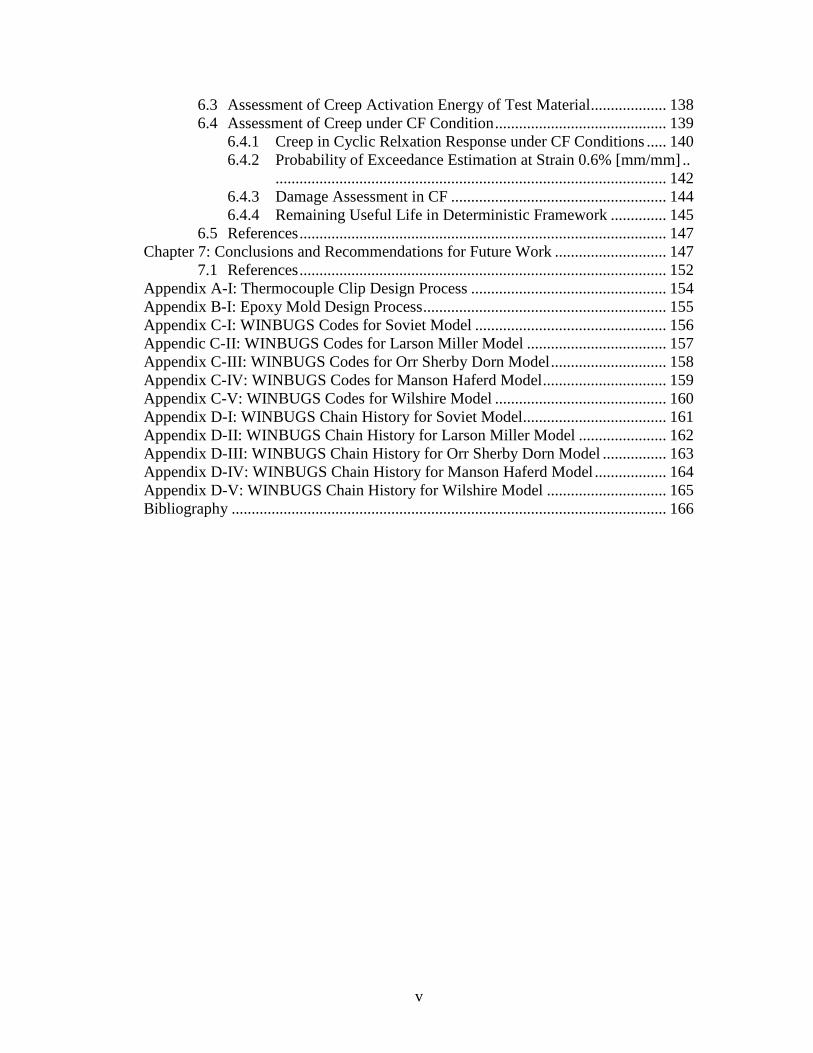
Table of Contents
Acknowledgements ....................................................................................................... ii
Table of Contents ......................................................................................................... iii List of Tables ............................................................................................................... vi List of Figures ............................................................................................................. vii
List of Symbols ........................................................................................................... xi Chapter 1: Introduction ................................................................................................. 1
1.1 Background .............................................................................................. 1
1.2 The Scope of The Thesis.......................................................................... 4
1.3 Thesis Organization ................................................................................. 6
1.4 References ................................................................................................ 7
Chapter 2: Literature Review ........................................................................................ 9
2.1 Introduction .............................................................................................. 9
2.2 Factors Affecting CF Life of Materials ................................................... 9
2.2.1 Microstructural Composition ....................................................... 9
2.2.1.1 Microstructural Composition ......................................... 9
2.2.1.2 Carbon Content ............................................................ 10
2.2.1.3 Effect of Heat Treatments on Ductility ........................ 10
2.2.2 Waveform and Frequency .......................................................... 11
2.2.3 Environemntal/Service Factors .................................................. 11
2.2.4 Complex Loading Path Histories ............................................... 12
2.2.5 Classical Creep Damage (voidage) ............................................ 12
2.2.5.1 Creep Curve ................................................................. 13
2.2.5.2 Creep Characteristics ................................................... 15
2.3 Published Studies on CF Expended Life Assesment of Materials ......... 17
2.4 Published Studies on Creep in Cyclic Relaxation Response ................. 24
2.5 Thesis Objective..................................................................................... 26
2.6 References .............................................................................................. 27
Chapter 3: Models for CF and Creep in Cyclic Relaxation Response in a Steel Alloy ..
................................................................................................................ 29
3.1 Introduction ............................................................................................ 29
3.2 Models for CF in Steels and Alloys ....................................................... 31
3.2.1 Loading Sequence Dependent CF Expended Life Model .......... 34
3.2.1.1 Sequential CF Loading ............................................... 34
3.2.1.1.1 Linear damage summation ......................... 34
3.2.1.1.2 Strain range partitioning ............................ 36
3.2.1.1.3 Frequency modified approach.................... 37
3.2.1.1.4 Damage rate model .................................... 38
3.2.1.1.5 Damage function method ........................... 39
3.2.1.1.6 Viscosity based model .............................. 41
3.2.1.1.7 Statistical thermal CF models ................... 44
3.2.1.1.7.1 Low cycle thermal fatigue
models ................................................................... 44
3.2.1.1.7.2 Leading creep rupture models46

iv
3.2.1.1.7.3 Combining Fatigue and Creep
Damages ................................................................... 50
3.2.1.2 Simultaneous CF Loading............................................ 51
3.2.1.2.1 Fii [ ] Model ............................................ 51
3.2.2 Case/Research Specific Alternate Approaches to CF Expended
Life Models .................................................................................................... 52
3.2.2.1 Generic Equation ......................................................... 53
3.2.3 CF expended life models when cyclic material data is not
available or not enough ............................................................................................... 58
3.2.3.1 Sequential CF loading .................................................. 58
3.2.3.2 Simultaneous CF loading ............................................. 58
3.2.4 Modified Robust Models for CF ................................................ 58
3.2.4.1 Comparisons of Modified Leading Models ................. 60
3.3 Creep Models in Cyclic Relaxation Response under CF Conditions ..... 62
3.3.1 Applicable Creep Models in Cyclic Relaxation Response under
CF Conditions .................................................................................................... 65
3.3.2 Comparisons of Modified Robust Models ................................. 68
3.4 References .............................................................................................. 69
Chapter 4: Experimental Details ................................................................................. 75
4.1 Introduction ............................................................................................ 75
4.2 Experimental Details .............................................................................. 75
4.2.1 Material ...................................................................................... 79
4.2.2 Tensile Test ................................................................................ 82
4.2.3 1D Uniaxial C Test .................................................................... 84
4.2.3.1 Rationale for Selection of CF Parameters .................... 87
4.2.3.2 1D Uniaxial CF Test Results ....................................... 93
4.3 References .............................................................................................. 99
Chapter 5: Estimation of empirical Parameters using Bayesian Inference ............... 101
5.1 Introduction .......................................................................................... 101
5.2 Estimation of Empirical Model Parameters Using Bayesian Inference104
5.2.1 Soviet Model ............................................................................ 106
5.2.2 Larson Miller Model ................................................................ 109
5.2.3 Orr-Sherby Dorn Model ........................................................... 113
5.2.4 Manson-Haferd Model ............................................................. 117
5.2.5 Wilshire Model ........................................................................ 121
5.3 References ............................................................................................ 125
Chapter 6: Assessment of CF and Creep in Cyclic Relaxation ............................... 127
6.1 Introduction .......................................................................................... 127
6.2 CF Expended Life Curves .................................................................... 128
6.2.1 Soviet Model ............................................................................ 128
6.2.2 Larson-Miller Model ................................................................ 130
6.2.3 Orr-Sherby Dorn ...................................................................... 131
6.2.4 Manson Haferd Model ............................................................. 133
6.2.5 Wilshire Model [Fii ( ) Model] .............................................. 134
6.2.6 Comparisons of CF Life Models.............................................. 136
v
6.3 Assessment of Creep Activation Energy of Test Material................... 138
6.4 Assessment of Creep under CF Condition ........................................... 139
6.4.1 Creep in Cyclic Relxation Response under CF Conditions ..... 140
6.4.2 Probability of Exceedance Estimation at Strain 0.6% [mm/mm] ..
.................................................................................................. 142
6.4.3 Damage Assessment in CF ...................................................... 144
6.4.4 Remaining Useful Life in Deterministic Framework .............. 145
6.5 References ............................................................................................ 147
Chapter 7: Conclusions and Recommendations for Future Work ............................ 147
7.1 References ............................................................................................ 152
Appendix A-I: Thermocouple Clip Design Process ................................................. 154
Appendix B-I: Epoxy Mold Design Process ............................................................. 155
Appendix C-I: WINBUGS Codes for Soviet Model ................................................ 156
Appendic C-II: WINBUGS Codes for Larson Miller Model ................................... 157
Appendix C-III: WINBUGS Codes for Orr Sherby Dorn Model ............................. 158
Appendix C-IV: WINBUGS Codes for Manson Haferd Model ............................... 159
Appendix C-V: WINBUGS Codes for Wilshire Model ........................................... 160
Appendix D-I: WINBUGS Chain History for Soviet Model.................................... 161
Appendix D-II: WINBUGS Chain History for Larson Miller Model ...................... 162
Appendix D-III: WINBUGS Chain History for Orr Sherby Dorn Model ................ 163
Appendix D-IV: WINBUGS Chain History for Manson Haferd Model .................. 164
Appendix D-V: WINBUGS Chain History for Wilshire Model .............................. 165
Bibliography ............................................................................................................. 166

vi
List of Tables
Table 1.1: Survey indicated summary of wave form usage for creep-fatigue testing ..5
Table 3.1: Review of creep-fatigue assessment methods in literature .........................33
Table 3.2: Relation between temperature and other parameters ..................................45
Table 3.3: Robust creep rupture models in literature ...................................................46
Table 3.4: Published creep models that describe the whole creep curve from primary
(P) to secondary (S) and tertiary part for 10Cr-Mo (9-10) steel alloys .......................66
Table 3.5: AIC values from comparison of different creep models for the given
experimental data .........................................................................................................68
Table 4.1: Standards used for specimen design and parameters of experimental tests76
Table 4.2: EDS chemical composition results .............................................................80
Table 4.3: Expected time to failures based on the Larson-Miller and Wilshire
formulas and equivalent test stress range .....................................................................87
Table 4.4: Summary of test parameters for 3 Fatigue-Creep Tests .............................89
Table 5.1: Data used for prediction of Wilshire Model for the test material .............122
Table 6.1: Soviet Model Bayesian parameters and their coefficient of variation ......129
Table 6.2: Larson-Model Model Bayesian parameters and their coefficient of
variation .....................................................................................................................130
Table 6.3: Orr-Sherby Dorn Bayesian parameters and their coefficient of variation 132
Table 6.4: Manson Haferd Model Bayesian parameters and their coefficient of
variation .....................................................................................................................133
Table 6.5: Wilshire Bayesian parameters and their coefficient of variation ..............135
Table 6.6: Activation energies for different hold-times at 675.15 (400 ) ............139
Table 6.7: Probability of exceedance at strain 0.6% [mm/mm] for different times at
CF test#3 (21min hold time) .....................................................................................144
Table 6.8: Cumulative creep damage in each creep-fatigue for 21min hold time creep-
fatigue test#3 ..............................................................................................................144
Table 6.9: Basic details of the service-aged secondary superheater ..........................146

vii
List of Figures
Figure 1.1: Structure of thesis ........................................................................................6
Figure 2.1: Typical creep curves showing the 3-stages of creep .................................14
Figure 2.2: Effect of applied stress on a creep curve at constant temperature ............ 16
Figure 3.1: Methodology for assessing integrity of structural components that operate
at high temperatures. TMF, thermo-mechanical fatigue; NDE, nondestructive
evaluation; LCF, low-cycle fatigue; HCF, high-cycle fatigue .................................... 30
Figure 3.2: Three classes of creep-fatigue life fraction models .................................. 31
Figure 3.3: Loading sequence dependent creep-fatigue expended life model ............ 32
Figure 3.4: Case/research specific alternate approaches to creep-fatigue extended life
models ................................................................................................................ 32
Figure 3.5: Creep-fatigue extended life models when cyclic material data is not
available ................................................................................................................ 33
Figure 3.6: Normalized reference stress (Fii) as a function of tCF for 316FR at
550 C ................................................................................................................ 60
Figure 3.7: Creep-fatigue model R2 for 316FR at 550 C .......................................... 61
Figure 3.8: Generic schematic of strain and stress history for a fully reversed strain
cycle with hold time at maximum tensile strain ......................................................... 61
Figure 3.9: Stress relaxation curves at three test temperatures in a 2.5% total strain
range ................................................................................................................ 65
Figure 3.10: R2 results for creep deformation in stress relaxation curves at 813 K test
temperature temperatures in a 2.5% total strain range ............................................ 69
Figure 4.1: Dimensions by ASTM E8/E8M-11 .......................................................... 76
Figure 4.2: Rounded dog-bone sample and rounded dog-bone sample placed in
particularly designed 316 stainless steel grips ............................................................ 77
Figure 4.3: (a) Designed 316 stainless steel grips for rounded dog-bone samples; (b) a
view from tension testing of a rounded dog-bone sample which is fixed on 647
Hydraulic Grips together with the particularly designed 316 stainless steels ............ 78
Figure 4.4: Creep furnace setup with thermocouples, and copper coil coolers; 316
stainless steel thermocouple clip attached to test specimen inside the creep furnace 78
Figure 4.5: Power supply unit of home-made creep furnace used to control the
furnace temperature .................................................................................................... 79
Figure 4.6: Automated polishing to provide a mirror-like quality on encapsulated
metal pieces ............................................................................................................... 80
Figure 4.7: Encapsulated 7x7 mm piece for EDS analysis after polishing ................ 80
Figure 4.8: (a) AFM picture of raw material surface in nanometer scale, (b) SEM
picture (1000x) of raw material surface in micrometer scale .................................... 81
Figure 4.9: (a) Fractured tensile specimen, (b) Dispersion of elements on the fractured
sample surface under SEM microscope ..................................................................... 81
Figure 4.10: (a) SEM picture for surface topography of 5min immersed steel alloy,
and (b) SEM picture of 15min immersed steel alloy ................................................. 82
Figure 4.11: MTS 810 test machine software and tension test inputs ....................... 83

viii
Figure 4.12: Tension test result in room temperature for the steel alloy ................... 83
Figure 4.13: (a)Ruptured dog-bone sample, and (b) Ductile cup and cone form of
ruptured cross-section of the steel alloy ..................................................................... 84
Figure 4.14: SEM pictures of the fracture surface of the uni-axial tensile test sample
(a) at 35x and (b) at 1000x showing the presence of surface pores ........................... 84
Figure 4.15: (a) ASTM E2714-09 creep-fatigue cycle shape: cycle with hold time at
control parameter peak in tension; (b) Adjusted creep-fatigue cycle shape according
to the available dog-bone sample design .................................................................... 86
Figure 4.16: Creep-fatigue test setting in Reliability and Mechanics lab ................... 86
Figure 4.17: Strain controlled creep-fatigue test cycle with stress Ratio = 0, and
Instron Dynamic Software Wave Matrix program steps. Step1 (tension), step2 (hold)
and step 3(release) ...................................................................................................... 90
Figure 4.18: Instron Dynamic Software WaveMatrix creep-fatigue test inputs: Step1 ..
................................................................................................................ 91
Figure 4.19: Instron Dynamic Software WaveMatrix creep-fatigue test inputs: Step2 ..
................................................................................................................ 91
Figure 4.20: Instron Dynamic Software WaveMatrix creep-fatigue test inputs: Step3 ..
............................................................................................................... 92
Figure 4.21: Instron Dynamic Software WaveMatrix test monitoring options ...........92
Figure 4.22: ASTM standard E2714-09 end-of-test criterion based on reduction of
peak stress for softening materials ...............................................................................93
Figure 4.23: Stress-strain hysteresis diagram for all cycles in 600 seconds hold time
creep-fatigue test in 673.15 (400 ) .........................................................................94
Figure 4.24: Strain-cycle to failure diagram for all cycles in 600 seconds hold time
creep-fatigue test in 673.15 (400 ) .........................................................................94
Figure 4.25: Stress-cycle to failure diagram for all cycles in 600 seconds hold time
creep-fatigue test in 673.15 ........................................................................95
Figure 4.26: Strain-cycle to failure for all cycles in 840 seconds hold time creep-
fatigue test in 673.15 (400 ) ...................................................................................95
Figure 4.27: Stress-cycle to failure diagram for all cycles in 840 seconds hold time
creep-fatigue test in 673.15 ........................................................................96
Figure 4.28: Strain-cycle to failure diagram for all cycles in 1260 seconds hold time
creep-fatigue test in 673.15 ) ........................................................................96
Figure 4.29: Stress-cycle to failure diagram for all cycles in 1260 seconds hold time
creep-fatigue test in 673.15 ........................................................................97
Figure 4.30: Test sample before and after CF test showing the visual impact of CF
deformation on the sample surface ..............................................................................97
Figure 4.31: Observed stress levels in each creep-fatigue test with respect to the
stress-strain curve in room temperature .......................................................................98
Figure 4.32: Observed number of cycles to failure with respect to the hold times in
each creep-fatigue test ..................................................................................................98
Figure 5.1: Bayesian inference framework ................................................................102
Figure 5.2: Normal distribution probability plot of failed creep-fatigue data ...........104
Figure 5.3: WinBUGS Bayesian Inference framework R2B results for each robust
creep-fatigue models ..................................................................................................105
Figure 5.4: WinBUGS node statistics for Soviet model ............................................107

ix
Figure 5.5: WinBUGS sample densities for parameters b0, b1 and b4 in Soviet Model
....................................................................................................................................108
Figure 5.6: WinBUGS correlation tool result between parameters b0,b1 and b4 in
Soviet Model ..............................................................................................................108
Figure 5.7: WinBUGS autocorrelation tool results for parameters b0,b1 and b4 in
Soviet Model ..............................................................................................................109
Figure 5.8: WinBUGS node statistics for Larson-Miller Model ...............................111
Figure 5.9: WinBUGS sample densities for b0,b1 and b2 in Larson-Miller Model ..111
Figure 5.10: WinBUGS correlation tool results between parameters b0,b1 and b2 in
Larson-Miller Model ..................................................................................................112
Figure 5.11: WinBUGS autocorrelation results for parameters b0,b1 and b2 in
Larson-Miller Model ..................................................................................................112
Figure 5.12: WinBUGS node statistics for Orr-Sherby Dorn Model ........................115
Figure 5.13: WinBUGS sample densities for b0,b1 and b2 in Orr-Sherby Dorn Model .
....................................................................................................................................116
Figure 5.14: WinBUGS correlation results between parameters b0,b1 and b2 in Orr-
Sherby Dorn Model....................................................................................................116
Figure 5.15: WinBUGS autocorrelation results for parameters b0,b1 and b2 in Orr-
Sherby Dorn Model....................................................................................................117
Figure 5.16: WinBUGS node statistics for Manson-Haferd Model ..........................119
Figure 5.17: WinBUGS sample densities for b0,b1 and b2 in Manson-Haferd Model ...
....................................................................................................................................120
Figure 5.18: WinBUGS correlation tool results between b0,b1 and b2 in Manson-
Haferd Model .............................................................................................................120
Figure 5.19: WinBUGS autocorrelation results between parameters b0,b1 and b2 in
Manson-Haferd Model ...............................................................................................121
Figure 5.20: WinBUGS node statistics for Wilshire Model ......................................123
Figure 5.21: WinBUGS sample densities for k and u in Wilshire Model .................124
Figure 5.22: WinBUGS correlation tool result between parameters k and u in
Wilshire Model ..........................................................................................................124
Figure 5.23: WinBUGS autocorrelation results for parameters k and u in Wilshire
Model .........................................................................................................................125
Figure 6.1: Soviet Model creep-fatigue expended life curve for steel alloy at
673.15 K (400 C ) ...................................................................................................129
Figure 6.2: Soviet-Model creep-fatigue 3D life graph for the steel alloy at 673.15 K
(400 C ) .....................................................................................................................130
Figure 6.3: Larson-Miller creep-fatigue expended life curve for the steel alloy at
673.15 K (400 C ) ...................................................................................................131
Figure 6.4: Larson-Miller Model creep-fatigue 3D life graph for the steel alloy at
673.15 K (400 C ) ...................................................................................................131
Figure 6.5: Orr-Sherby Dorn Model creep-fatigue expended life curve for the steel
alloy at 673.15 K (400 C ) ......................................................................................132
Figure 6.6: Orr-Sherby Dorn Model creep-fatigue 3D expended life graph for the
steel alloy at 673.15 K (400 C ) ...............................................................................133
Figure 6.7: Manson Haferd Model creep-fatigue expended life curve for the steel
alloy at 673.15 K (400 C ) .......................................................................................134

x
Figure 6.8: Manson Haferd Model creep –fatigue 3D expended life graph for the steel
alloy at 673.15 K (400 C ) .......................................................................................134
Figure 6.9: Wilshire Model creep-fatigue expended life curve for the steel alloy at
673.15 K (400 C ) ....................................................................................................135
Figure 6.10: Wilshire Model creep-fatigue 3D expended life graph for the steel alloy
at 673.15 K (400 C ) ................................................................................................136
Figure 6.11: Time to creep-fatigue failure comparison for the steel alloy ................136
Figure 6.12: Predicted vs. observed creep-fatigue life for the steel alloy ..................137
Figure 6.13: R2 results for Norton Bailey, Nuhi’s Empirical and Modified Theta
Models........................................................................................................................141
Figure 6.14: Creep curves in cyclic relaxation response under creep-fatigue
conditions for 10min (CF Test#1), 14min (CF Test#2), and 21min (CF Test#3) hold
times at 673.15 K (400 C ) .......................................................................................142
Figure 6.15: Normal cdf at strain 0.006 [mm/mm] for creep in cyclic relaxation
response under creep-fatigue conditions for 10min (CF Test#1), 14min (CF Test #2)
and 21min (CF Test #3) hold times at 673.15 K (400 C ) .......................................143
Figure 6.16: Acceleration factor graph with respect to the specified use level stress
17.3MPa .....................................................................................................................146
Figure A-I.1: (a) Thermocouple clip attached to test sample, and (b) thermocouple
clip design dimensions ...............................................................................................154
Figure B-I.1: (a) Epoxy mold produced, and (b) mounted sample using epoxy mold
....................................................................................................................................155

xi
List of Symbols
D total creep-fatigue damage
n number of applied cycles at a particular loading condition
Nf number of cycles to failure at a particular strain range
t time duration at a particular load condition
tr time to rupture from isothermal stress-rupture curves for a given loading condition
plastic-plastic
creep-plastic
plastic-creep
creep-creep
C material parameter
material parameter
compression-going frequency
tension-going frequency
material constants
creep-fatigue expended life model parameters i=1,2,3,4,5
cycle period
time per cycle of continuous loading
compression hold time
tension hold time
minimum creep rate
creep life
stress

xii
T temperature
activation energy
fatigue damage
creep damage
reference stress
normalized reference stress
S strain range parameter
R strain rate parameter
T temperature parameter
H hold parameter
duration of hold time in hours
strain rate
elastic strain
plastic strain
E Elastic modulus
stress relaxation rate
time to creep-fatigue failure
change in initial length
initial length
linear expansion coefficient
change in temperature
initial temperature

xiii
final temperature
apparent activation energy
CF creep-fatigue
LCF low-cycle fatigue
HTLCF high temperature low cycle fatigue
R2B Bayesian Pearson coefficient of determination
R2 Pearson coefficient of determination
LS loading sequence
MCMC Markov Chain Monte Carlo

1
Chapter 1: Introduction
1.1 Background
Historically, the earliest attempts to evaluate combined creep and fatigue
properties were made in Germany by Hempel and his coworkers [1, 2-4] during 1936-
42 [1] focusing mainly on carbon steels. At about the same period, Tapsell and his co-
workers [5,6] at the National Physical Laboratory studied the behavior of steels and
extended their studies to develop methods of predicting combined creep and fatigue
(CF) behavior [1].
Since the Second World War, a great deal of effort has been devoted in the
United States to evaluate combined CF properties of a wide range of existing alloys in
particular high temperature alloys. In the United Kingdom, commercial alloys have
been examined at Bristol-Siddeley Engines Ltd., by Frith [7], with special reference
to fatigue-rupture properties [1].
Perhaps the first attempt to apply basic structural theories to the problem of
combined CF was made by Kennedy [8] at the British Iron and Steel Research
Association, London. There is now an increased awareness of the importance of
testing under combined CF conditions, and this is reflected by the number of testing
and research programs at several alloy manufacturers and end-user facilities.
Meleka [1] presented some examples of cases where combined CF stresses are
met with under service conditions. In almost all high-temperature applications,
simultaneous CF may occur, even in normally static applications. Most of the
following are suggested in Ref.[1] as examples of cases where combined CF are met
under service conditions.

2
a. Turbine Blades: Turbine blades are subjected to severe service conditions and
combined fatigue-creep is a major source of turbine failure. The blade is
subjected to direct tensile stresses as a result of the centrifugal forces
produced by the high speed rotation of the blade. Bending fatigue stresses are
also present, mainly owing to the mechanical resonance of the blade. Turbine
blades may fail by creep or by fatigue, depending on the relative severity of
stresses. More combined CF data on turbine-blade materials exists than on any
other, mainly because of the critical nature of the function of these
components.
b. Nuclear Power Applications: Magnesium alloys are used extensively as
cladding nuclear fuel elements, chiefly because of their low neutron-
absorption. The cladding is exposed to temperatures up to 500 and must
exhibit sufficient creep strength and ductility to accommodate the dimensional
changes of the uranium element and also to support its weight in a vertically
stacked array. Similar conditions also apply to structural components inside
the reactor. Creep stresses are obviously present because of the load-carrying
function of the component, and fatigue stresses are produced by the vibrations
resulting from gas flow. Separate CF have been conducted on a number of
magnesium alloys separately, but very limited data exists for combined CF
tests.
c. Components in Power Generation Plants: High temperature components in
power generation are subjected to load cycles that involve gradually
accumulating and life-limiting damage from cyclic (fatigue) and more steadily
3
progressing (creep) mechanisms of deformation and fracture. As a
consequence, resistance of structural materials to combined CF is of
considerable interest for both design and life assessment. In many applications
of power generation, the loading rates and cycling frequencies are low, so that
the combined CF damage could be creep dominated [10].
d. The Supersonic Airliner: One of the important factors to be considered in the
design of a supersonic airliner is the effect of kinetic heating on the strength of
the structure. Temperatures up to 150 may be encountered, resulting in
creep deformation. This will have to be limited to small values, say 0.1% over
the life of airliner. So far, designers have based their calculations for present-
day airliners on room-temperature fatigue data, but in the presence of kinetic
heating creep considerations will also have to be taken into account.
e. Jet and Rocket Engines: Service conditions in jet and rocket engines are quite
severe because of the high stress and temperatures encountered during service
life. Under steady operating conditions the various components are subjected
to essentially creep stresses, but severe vibration may be represented for short
times which may affect the creep characteristics of the components.
f. Pipes in Steam Power Plant: These pipes are normally designed on the basis
of creep, although from a study of fracture characteristics certain failures have
been traced to fatigue. Large fatigue stresses are produced in power plant
pipes by the vibrations in rotating machinery. During the design or service of
such pipes, attention should be given to reducing the possibility of excessive
vibrations.
4
g. Relaxation of Internal Stresses: The relaxation of internal stresses during
service may lead to dimensional distortion of component concerned.
Relaxation is, of course, another form of creep deformation, where the locked-
in stresses give way to plastic deformation by creep. Relaxation under some
circumstances can be initiated or accelerated by the presence of fatigue
stresses.
h. Thermal Fatigue: It is clear that thermal-cycling conditions may have effects
on creep properties similar to those caused by mechanical fatigue. One or two
examples of this is given in Ref.[9].
1.2 The Scope of the Thesis
The development of CF damage is influenced by temperature, strain amplitude,
strain rate and hold time, and the creep strength and ductility of the material. With
increasing hold time (and/or decreasing strain rate) and decreasing strain amplitude at
high temperatures, the creep damage becomes more and more important. A survey
was conducted using 57 high temperature fatigue testing specialists in 13 countries to
study current CF testing practices concerning: the types of test employed, test piece
machines and loading, strain measurement, temperature measurement and data
acquisition.
CF damage may be generated in tests involving sequential blocks of CF
loading. However, from the results of the survey, it was more common to apply a
waveform shape responsible for the generation of both static and transient loading
within the same cycle. CF tests were performed in both load and strain control,
although more commonly in strain control (see, Table 1.1). The most commonly

5
adopted CF waveform was a cycle involving one or more hold times, where hold
periods could be anything between 1 min and 24h (with an extreme case of 90 days).
Table 1.1: Survey indicated summary of waveform usage
for CF testing [11]
Waveform Load Control
(User %)
Strain Control
(User %)
Low frequency triangular
(isothermal) 14 59
Saw tooth triangular (isothermal) 27 68
Cyclic hold (isothermal) 32 86
Thermo-mechanical fatigue (TMF)
(without and with hold time) 14 68
The most widely used test specimen type was a uniform parallel gauge section
specimen (without ridges for extensometer fixation), although other specimen types
were used for special circumstances. Despite a uniform test specimen type, a range of
gauge section dimensions and end connections were employed.
A range of failure criteria were adopted, varying between 2% and 25%
reductions in steady state maximum stress. Notably, the most commonly adopted
criteria was a 10% reduction in maximum stress (45%) compared with the anticipated
outcome of a 2% reduction (22%).
In order to come up for a CF testing procedure for this thesis work, the
worldwide survey results of current practices conducted by EPRI have been reviewed.
These results have generated the motivation for this thesis work. Addressing the
prediction feasibility of the all CF models identified in Chapter 3 is beyond the scope
of this thesis. Hence, the main focus in this study is isothermal CF tests under strain
control with stress ratio R=0 and hold periods in tension, and prediction feasibility
of CF expended life models which do not need separation in CF damage.

6
Therefore, effective CF expended life was predicted utilizing the creep rupture
properties of a material. Consequently, creep deformation produced by hold times
in tension enabled this research to evaluate creep damage assessment in cyclic
relaxation response in CF tests performed.
1.3 Thesis Organization
The structure of this thesis is presented in Figure 1.1.:
Figure 1.1: Structure of thesis
The thesis is organized as follows:
In Chapter 2, an introduction to factors influencing CF in steel materials such as
metallurgical state, waveform and frequency, environment (e.g. oxidation), complex
loading path histories, classical creep damage (voidage) is presented first, followed
7
by a literature review on CF in steels and alloys. Subsequently, a literature review on
creep in cyclic relaxation response is presented.
In Chapter 3, models are adjusted into CF problem under uniaxial interaction. Best
possible creep models are evaluated for creep deformation in cyclic relaxation
response.
In Chapter 4, CF experiments are presented and experimental details are given.
In Chapter 5, experimental results are evaluated in Bayesian inference framework
with respect to the models concerned in Chapter 3. Details of WinBUGS codes which
uses MCMC to fit statistical models, and steps to reach correct posterior distributions
are presented.
In Chapter 6, experimental results are presented by posterior distributions proposed
in the previous Chapter 5, and compared to validate the models discussed in Chapter
3.
In Chapter 7, conclusions based on the results of this research are presented
followed by future recommendations.
1.4 References
[1] Meleka, A.H., “Combined creep and fatigue properties,” Metallurgical
Reviews, Vol.7, Issue:25, 1962.
[2] Hempel, M. and Tillmanns, H.E., Mitt. K.-W.Inst.Eisenforsch, Vol.18,
Issue:163, 1936.
[3] Hempel, M. and Ardelt, F., ibid., Vol.21, Issue:115, 1939.
[4] Hempel, H. and Krug, H., ibid., Vo.24, Issue:77, 1942.
[5] Tapsell, H.J., Forrest, P.G., and Tremain, G.R., Engineering, Vol.170,
Issue:189, 1950.
8
[6] Tapsell, H.J., “Symposium on High-Temperature Steels and Alloys for Gas
Turbines” (Special Rep. No.43), p:169, London (Iron and Steel Inst.), 1952.
[7] Frith, P.H., “Properities of Wrought and Cast Aluminum and Magnesium
Alloys at Room and Elevated Temperatures,” London (H.M. Stationery
Office), 1956.
[8] Kennedy, A.J., “Proceedings of the International Conference on Fatigue of
Metals,” p:401, London(Inst. Mech. Eng.), 1956.
[9] A.S.T.M., “Symposium on the Effect of Cyclic Heating and Stressing on
Metals at Elevated Temperatures,” (Special Tech. Publ. No.165),
Philadelphia, Pa. (Amer. Soc. Test. Mat.), 1954.
[10] Holmstrom, S., Auerkari, P., “A robust model for creep-fatigue life
assessment,” Mechanical Science and Engineering A, Vol.559, pp:333-335,
2013.
[11] Holdsworth, S.R., Gandy, D., “Towards a standard for creep-fatigue
testing,” Advances in Materials Technology for Fossil Power Plants
Proceedings from the Fifth International Conference, In. Viswanathan, R.,
Gandy, D., and Coleman, K. (Eds.), pp: 689-701, 2008.

9
Chapter 2: Literature Review
2.1 Introduction
Chapter 2 presents four sub-sections linked to one another. Section 2.2 presents
factors affecting creep-fatigue (CF) life of material. Section 2.3 and 2.4 present
published studies on CF expended life assessment of materials, and creep in cyclic
relaxation response. Section 2.5 specifies the thesis objectives in bullet points
regarding the reasoning provided in Section 1.2 and reviews presented in Section 2.3.
2.2 Factors Affecting CF Expended Life of Materials
Strain-controlled fatigue tests of annealed 2.25Cr-1Mo steel results from
strain-controlled fatigue tests conducted in various environments from 370 to 593
have shown that the time-dependent fatigue lifetime depends on the influence of (1)
metallurgical state, (2) waveform and frequency, (3) environment (e.g. oxidation), (4)
complex loading path histories, and (5) classical creep damage (voidage) [1]. In
following sub-sections each of these influences is explained.
2.2.1 Metallurgical State
Metallurgical state is separated in to three sub-sections in this study. These are
microstructural composition, carbon content, and effect of heat treatments on
ductility. They are explained in following.
2.2.1.1 Microstructural Composition
Heat to heat variations has been reported in time-dependent fatigue properties
of type 304 stainless steel. Small grain sizes and the presence of fine closely packed

10
integranular precipitates have both improved the cyclic life. Intergranular precipitate
restricts grain-boundary sliding and hence limits wedge cracking. Although grain size
does not impact continuous-cycle fatigue life in the low-cycle regime, time-dependent
fatigue behavior at the indicated temperature is improved as the grain size is
decreased [1]. Qualitatively, the time dependent fatigue behavior of types 304 and
316 stainless steel are directly related to the creep ductility at strain rates similar to
those that occur during stress relaxation [1].
2.2.1.2 Carbon Content
In Japan, type 304 stainless steel used in a prototype reactor, Monju is being
replaced with low-carbon and nitrogen-controlled 316FR (fast reactor). The reduced
carbon content of 316FR leads to considerably better creep strength than the
conventional type 316 steel by reducing the Chromium Carbide precipitation along
grain boundaries, which promotes initiation of creep cavities [2].
2.2.1.3 Effect of Heat Treatments on Ductility
Solution heat treatment (1250 , 16h) prior to rolling reduces the possibility
of carbide precipitation by homogenizing chromium distribution [2]. Consider 2
plates, A and B that were both produced using hot-rolling. The heat treatment of
Plate A was 1050 for 30 min followed by water quenching. Plate B had the same
treatment as Plate A plus an additional treatment at 1250 for 16h to homogenize
chromium distribution. Under the same test conditions, plate A showed a shorter life
than plate B. This trend coincides with the fact that ductility in creep tests has a
strong correlation between creep ductility and CF life [2].
11
2.2.2 Waveform and Frequency
It was reported in past studies that tensile loading leads to larger life reduction
than compressive loading for austenitic stainless steel, and this was confirmed with
several tests for the tested material [2].
At least two specific mechanisms can lead to intergranular crack formation and
fracture in polycrystalline steels. These include formation of intergranular creep
cavities and by grain-boundary triple-point nucleation of voidage as a result of
localized grain-boundary sliding. The latter mechanism usually occurs at higher
stresses (approaching the yield strength), which occur in low-to intermediate-cycle
fatigue applications. Under tensile loads held at elevated temperatures high enough
for creep to occur, intergranular voids form easily which in turn favors intergranular
fatigue crack propagation. Increasing the temperature within the creep range or
decreasing the cyclic frequency further weakens the grain boundaries with respect to
the intragranular matrix material and promotes grain boundary sliding, resulting in
decreased cyclic life for a given specimen geometry [1].
2.2.3 Environmental/Service Factors
It is known that constant loading at high-temperature reduces the number of
cycles to failure from pure-fatigue loading due to “creep damage” or other
mechanisms such as oxidation [2]. Failure life at 600 tended to be shorter than that
at 550 , but the difference was much smaller than observed in pure-creep tests. The
difference of controlled parameters, i.e., stress-versus strain, is the reason for this [2].

12
2.2.4 Complex Loading Path Histories
For 304 stainless steel, previous studies have performed strain-controlled hold
time tests with the strain held at the peak strain amplitudes. The following
conclusions can be made from these results [1]:
1. Tensile hold times at peak strain values are more damaging than
compressive hold times of equal duration.
2. Hold periods imposed at other locations on the hysteresis loops, such as at
zero stress or zero relaxation points, degrade fatigue life but not as much as
hold periods imposed at peak tensile strain values.
3. Hold periods imposed on the tension-going side of the loop tend to be more
detrimental than those imposed on the compression-going side.
4. The rate of accumulation of a given amount of relaxation or creep strain is
important in that lower creep rates favor intergranular cavitations and
hence result in lower fatigue lives.
2.2.5 Classical Creep Damage (voidage)
Creep is modeled as time-dependent deformation, and thereby is
mathematically distinct from elastic and plastic deformation. Elastic and plastic
deformations are mathematically modeled as instantaneous deformations occurring in
response to applied stresses. In reality, all deformations are time dependent, but the
characteristic times for elastic and plastic deformations are orders of magnitude
smaller than those for creep [7].
At elevated temperatures, most materials can fail at a stress which is much
lower than its ultimate strength measured at ambient temperature. These failures are

13
time-dependent and are caused by creep rupture [7]. More generally, materials
undergoing continuous deformation over time under a constant load or stress are said
to be creeping. Elastic, plastic, visco-elastic and visco-plastic deformations can all be
included in the creep process, depending on the material and the characteristic time of
the deformation. However, creep deformation is often treated as plastic deformation
because the failures associated with creep are similar to those due to yielding in
plastic deformation of materials. There are various mechanisms of creep in materials
at elevated temperatures and thus there are different creep models. These mechanisms
are often be inter-related, depending on the material [7]. The measurement of
phenomenological creep of materials is quite simple, although the mechanisms of
creep are complicated [7].
2.2.5.1 Creep Curve
A creep curve shows time dependent deformation under constant load. When
a constant load is applied to a tensile specimen at a constant temperature (usually
greater than 0.4 ~ 0.5 of the absolute melting temperature of the specimen) the strain
of the specimen is determined as a function of time. A typical variation of creep strain
with time in a specimen at a constant load is schematically shown as curve A in
Figure 2.1. The slope of the curve is the creep rate. Creep is usually characterized as
having three distinct stages, as reflected by the creep curve. Stage 1 of curve A,
follows after an initial instantaneous strain , which includes elastic and plastic
deformations. During phase 1, the creep rate decreases with time. This is termed
primary creep. Stage 2 of curve A during which the creep rate approaches a stable
minimum value, relatively constant over time, is secondary creep or steady-state

14
creep. The creep rate in the secondary creep stage, often termed the steady-state creep
rate, is an important engineering property because most deformations involve this
stage. In stage 3, termed tertiary creep, the creep rate accelerates with time accelerates
with time and usually leads to failure by creep rupture. Although the three stages
represent the creep behavior in most materials, the primary creep stage can be absent
for some materials. The extension during the tertiary creep stage can be limited in
brittle materials and very extensive in ductile materials [3].
Figure 2.1 Typical creep curves showing the 3-stages of
creep [3]
Curve B in Figure 2.1 is for a creep test with a constant stress. Under a
constant load, the axial stress increases with time because the specimen decreases in
cross-sectional area. The increasing stress thus accelerates creep and causes strains in
the tertiary phase, as shown in curve A. In most engineering creep tests, it is often
easier to maintain a constant load during the test because of instrumentation
limitations. Under constant-stress, as shown in curve B, steady-state creep dominates
over a much longer time period and thus greatly postpones tertiary creep [3].

15
2.2.5.2 Creep Characteristics
Creep characteristics depend on several factors such as time, temperature,
stress and the micro-structure [3]. These factors are explained in the following
sections.
a. Time
A time scale is always involved in creep. For most engineering materials
tested at low temperatures, the measured tensile properties are relatively independent
of the test time, regardless of whether it is 5 minutes or 5 hours. If time dependence is
observed in a tensile test, the material is by definition creeping. The main reason for
this time dependence is the involvement of thermally activated time-dependent
processes. Creep tests are designed to last hours, days or even years where the overall
creep rate is usually controlled by a single dominant thermally activated process. For
example, if the controlling process is diffusional, the creep rate is called diffusion
controlled [3].
b. Temperature
Creep mechanisms involve mechanisms at the atomic scale. At higher
temperatures, the mobility of atoms or vacancies increases rapidly with temperature
so that they can diffuse through the lattice of the materials along the direction of the
hydrostatic stress gradient, which is called self-diffusion. The self-diffusion of atoms
or vacancies can also help dislocations climb. At low temperatures, creep becomes
less diffusion-controlled. Diffusion can occur, but is limited in local porous areas, like
grain boundaries and phase interfaces, which is called grain-boundary diffusion.
Since creep is strongly temperature dependent, a measurement of this temperature
16
dependence is important. A temperature which is considered high for creep in one
material might not be so high in another. To compensate for this difference,
temperature is often expressed on a homologous scale, the ratio of the test
temperature (T), to the melting temperature (Tm) of the material on an absolute
temperature scale. Generally, creep becomes of engineering importance at T > 0.5Tm.
This should be regarded as an approximate empirical guideline based on the
observations that above 0.5Tm, creep is most likely to be governed by mechanisms
that depend on self-diffusion.
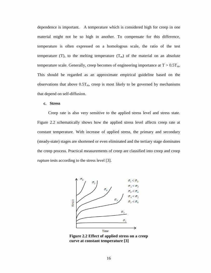
c. Stress
Creep rate is also very sensitive to the applied stress level and stress state.
Figure 2.2 schematically shows how the applied stress level affects creep rate at
constant temperature. With increase of applied stress, the primary and secondary
(steady-state) stages are shortened or even eliminated and the tertiary stage dominates
the creep process. Practical measurements of creep are classified into creep and creep
rupture tests according to the stress level [3].
Figure 2.2 Effect of applied stress on a creep
curve at constant temperature [3]

17
Creep tests are carried out at low stresses to avoid tertiary creep. The purpose
of creep tests is mostly to determine the steady-state creep rate. The total strain is
often less than 0.5% [3]. Creep rupture tests are similar to creep tests except that high
loads are applied to precipitate failure of the material. Creep rupture tests are mostly
used for obtaining the time-to-failure at a given stress and a given temperature. The
total strain can be as high as 50% [3].
Different stress states such as, such as simple tension, simple compression,
simple shear, simple torsion, and in some special cases, multi-axial stresses can be
used for creep tests and creep rupture tests,. The difference in the results at the same
stress level in simple tension and simple compression indicate the sensitively of the
creep rate to the direction of stress. The creep rate for lead and nickel, for example, is
greater in tension than in compression. Cyclic stress also affects creep rate. At low
creep temperatures, the steady-state creep rate is increased in many metallic materials
by cyclic stresses while the opposite is often found at high creep temperatures [3].
2.3 Published Studies on CF Expended Life Assessment of Materials
The literature review below covers peer reviewed articles from 1976 to 2013.
Efforts in CF expended life models development are presented in chronological order.
Ostergen [4] developed an approach for predicting strain-controlled, low
cycle fatigue life at elevated temperature using a proposed energy measure of fatigue
damage. This measure of damage, defined as the net tensile hysteretic energy of the
fatigue cycle, can be approximated by the damage function where ( is
the maximum stress in the cycle and is the inelastic strain range. The damage
function was applied to predict the effects of hold time and frequency, when time

18
dependent damage occurs, through failure relations incorporating a variation of
Coffin’s frequency modified approach. Failure equations were developed for two
postulated categories of time dependent damage.
Halford et al. [5] presented procedures based on strain range partitioning (SRP)
for estimating the effects of environment and other influences on the high
temperature, low-cycle, CF resistance of alloys. It was proposed that the plastic and
creep ductilities determined from conventional tensile and creep-rupture tests
conducted in the environment of interest be used in a set of ductility normalized
equations for making a first order approximation of the four (SRP) inelastic strain
range–life relations. Different levels of sophistication in the application of the
procedures were presented by means of illustrative examples with several high
temperature alloys. Predictions of cyclic lives generally agreed with observed lives
within factors of three.
Lloyd and Wareing [6] attempted to extend such models to cover the situations
in which creep damage is introduced during periods of stress relaxation. Equations
predicting fatigue life as a function of hold period are in good agreement with
experimental data, for Type 316 stainless steel and Incoloy-800. Components
operating at elevated temperature are often subjected to complex strain-time histories
which include periods of cyclic strain, creep strain and relaxation strain resulting
from the conversion of elastic strain to plastic strain. It has become increasingly
apparent that one of the most damaging strain time patterns is when the strain is held
constant at the maximum tensile strain part of a high strain fatigue cycle. To predict
the life of a plant operating under such conditions is essential to understand the

19
mechanisms by which fracture development occurs. To this end, models have been
developed which successfully describe the behavior of materials subjected to simple
cycling at both room and elevated temperature. Wareing [6] described such cycles
and extended it to cover cycles containing periods of stress relaxation. The
predictions arising from such models were compared with experimental data on three
austenitic steels at temperatures from 538 to 760 .
Brinkman [1] reviewed the effects of various phenomena such as creep-
induced intergranular cavitation, mean stress material condition, and environment on
the fatigue life of several engineering structural alloys. Materials used to illustrate
these effects when subjected to various loading conditions within the creep range
included 2.25Cr-1Mo steel (annealed), modified 9Cr-1Mo steel (normalized and
tempered), types 304 and 316 stainless steel, alloy 800H, Hastelloy X, and alloy 718.
Several models were used to extrapolate available data to predict life were also
discussed in terms of both their strengths and apparent shortcomings. No model was
clearly superior in its ability to predict life for all alloys under all loading conditions
envisioned, particularly at low strain ranges with long creep hold periods which
occurs in many applications.
Fatemi and Yangth [7] provided a comprehensive review of cumulative
fatigue damage theories for metals and their alloys, emphasizing the
approaches developed between the early 1970s to the early I990s. These
theories were grouped into six categories: linear damage rules; nonlinear
damage curve and two-stage linearization approaches; life curve modification
methods; approaches based on crack growth concepts; continuum damage

20
mechanics models; and energy-based theories.
Goswami, [8] reviewed the dwell sensitivity behavior and mechanisms
controlling deformation and failure under high-temperature low cycle fatigue
(HTLCF) conditions for a range of materials. Dwell sensitivity maps were
constructed utilizing normalized cycle ratio (NCR) and strain levels. The trends
identified were summarized as follows:
1. Dwell cycles were beneficial to the creep–fatigue resistance only in
isolated cases for copper alloys; AMZIRC and NARaloy-Z, and
superalloys;
2. PWA 1480 and MA 754 an (ODS) alloy. Solders (96.5 Pb–3.5 Sn and 37 Pb–
63 Sn), copper alloys; AMZIRC and NARaloy-Z, low steel alloys; 1 Cr-Mo-
V, 1.25 Cr-Mo and 9 Cr-1 Mo, stainless steels; SS 304, SS 304L, SS 316, and
SS 316L, superalloys; Mar M 002, Rene 80, Inconel 617, IN 100, PWA 1480
and MA 754 were observed to be tensile dwell sensitive.
3. Low steel alloy 2.25 Cr-Mo, titanium alloys Ti-6 Al-4V and IMI 829 and
superalloys Mar M 002 below 1040 C, Waspaloy and Rene 95 were found to
be compressive dwell sensitive.
Goswami [8] predicted the dwell sensitivity fatigue behavior empirically
relating the strength ratios with ductility ratios. It was proposed that when the
ductility ratio was equal to the strength ratio, compressive dwell sensitivity
occurred and for unequal conditions, tensile dwell sensitivity occurred. These
factors were determined and dwell sensitivity predicted. The mechanisms
controlling deformation and failure were categorized as follows: Each cycle
21
type produced deformation in either transgranular (TG), mixed, or intergranular
(IG) mode. Cyclic softening resulted in IG deformation as the stresses reduced.
Grain boundary sliding, cavity formation and oxidation damage interacted and
reduced life faster than TG modes, in which striations were observed. Depending
upon the cycle time, stresses, and temperature, deformation in terms of
precipitation, slip patterns, carbides, depletion of chromium carb ides , Cr-Mo
clusters occurred. These resulted in IG corrosion, oxidation and creep–fatigue
interactions causing additional damage. Dynamic strain aging occurred depending
upon the microstructure, temperature and material composition. Precipitates
developed which enhanced HTLCF resistance, however, other competition
mechanisms under dwell conditions were not known. The dwell sensitivity behavior
and mechanisms controlling deformation and failure of numerous materials were
summarized in this paper.
Goswami and Hannien [9] examined mechanisms controlling deformation
and f a i l u r e under high temperature CF conditions. The materials studied
were pure alloys, solder alloys, copper alloys, low steel alloys, stainless steels,
titanium alloys, tantalum alloys, and Ni-based alloys. The deformation and
failure mechanisms, f a t i g u e , creep, oxidation and their interaction, varied
depending on the test and material parameters employed. Deformation
mechanisms, such as cavity formation, grain boundary sliding, intergranular and
transgranular damage, oxidation, internal damage, dislocation cell formation, and
other damage mechanisms are very important in order to gain knowledge of
fatigue behavior of materials. The observed mechanisms can be categorized as

22
follows:
1. Depending on the test parameters employed, a high NCR resulted in high
strain levels. The damage was due to CF interaction by mixed TG and IG
cracking, creep damage by cavity formation and surface damage by oxidation.
Oxidation damage was found to depend on a critical temperature and
compression and tension dwell periods in a cycle.
2. Dwell sensitivity was effective only below a certain strain range, and once this
threshold was exceeded NCR value was not affected with a further increase in
dwell time.
3. Microstructures changed depending on test temperature, dwell time, and strain
range. Triple point cracking and cavities formed as a result. New precipitation
occurred depending on temperature, strain range and dwell time. Some
precipitates were beneficial in blocking the grain boundary damage,
whereas other precipitates changed the dislocation substructure promoting
more damage.
4. Depleted regions on the grain boundaries developed due to exposure at high
temperatures resulting in the formation or propagation of IG cracks.
5. Dwell evolved mean stresses in tension and compression directions. Mean
stress in tension was more detrimental and caused dwell sensitivity.
6. Dwell sensitivity was also dependent on material condition and defects
present in the material.
Goswami [10] presented a data bank that was compiled from published and
unpublished sources. Using this data, low cycle fatigue curves were generated

23
under a range of test conditions showing the effect of test parameters on the Coffin–
Manson behavior of steel alloys. Phenomenological methods of creep–fatigue life
prediction were summarized in a table showing number of material parameters
required by each method and type of tests needed to generate such parameters.
Applicability of viscosity method was assessed with creep–fatigue data on 1Cr–
Mo–V, 2.25Cr–Mo and 9Cr–1Mo steels. Generic equations were developed in this
paper to predict the creep–fatigue life of high temperature materials. Several new
multivariate equations were developed to predict the creep–fatigue life of following
alloy groups; (1) Cr–Mo steels, (2) stainless steels and (3) generic materials
involving the materials from the following alloy groups, solder, copper, steels,
titanium, tantalum and nickel-based alloys. Statistical analysis was performed in
terms of coefficient of correlation (R2) and normal distribution plots and
recommended these methods in the design of components operating at high
temperatures.
Takahashi et al. [11, 12] developed a CF evaluation method for low-carbon,
nitrogen-controlled 316 stainless steel, 316FR. To develop a CF evaluation method
suitable for this steel, a number of uniaxial CF tests were conducted for three
products of this steel. Long-term data up to about 35,000 h was obtained and the
applicability of failure life prediction methods was studied based upon their results.
Cruciform shaped specimens were also tested under biaxial loading conditions to
examine the effect of stress multiaxiality on failure life under CF condition.
He [13] investigated the creep fatigue behavior of stainless steel materials. In
the low cycle thermal fatigue life model, Manson’s Universal Slopes equation was

24
used as an empirical correlation which relates fatigue endurance to tensile properties.
Fatigue test data was used in conjunction with different models to establish the
relationship between temperature and other parameters. Then statistical creep models
were created for stainless steel materials. In order to correlate the results of
accelerated life tests with long-term service performance at more moderate
temperatures, different creep prediction models, namely the Basquin model and
Sherby-Dorn model, were studied. Comparison between the different creep
prediction models were carried out for a range of stresses and temperatures. A linear
damage summation method was used to establish life prediction model of stainless
steels materials under fatigue creep interaction.
Holmström and Auerkari [14] stated high temperature components subjected
to long term cyclic operation will acquire life-limiting damage from both creep and
fatigue. A new robust model for CF life assessment was proposed with a minimal set
of fitting constants, and without the need to separate creep and fatigue damage or life
fractions. The model is based on the creep rupture behavior of the material with a
fatigue correction described by hold time (in tension) and total strain range at
temperature. The model is shown to predict the observed CF life of ferritic steel P91,
austenitic steel 316FR, and Ni alloy A230 with a scatter band close to a factor of 2.
2.4 Published Studies on Creep in Cyclic Relaxation Response
Jaske et al. [16] made a detailed analysis of data from low-cycle fatigue tests of
solution-annealed nickel-iron-chromium Alloy 800 at 1000, 1200, and 1400 °F and of
Type 304 austenitic stainless steel at 1000 and 1200 °F with hold times at maximum
tensile strain. A single equation was found to approximate the cyclically stable stress

25
relaxation curves for both alloys at these temperatures. This equation was then used to
create a linear time fraction creep damage analysis of the stable stress relaxation
curves, and a linear life fraction rule was used to compute fatigue damage. CF
damage interaction was evaluated for both alloys using the results of these damage
computations. The strain range was found to affect the damage interaction for Type
304 stainless steel but not for the Alloy 800. With increasing hold times, both creep
and total damage increased for the Alloy 800, decreased for the Type 304
stainless steel, and the fatigue damage decreased for both alloys. A method was
developed to relate the length of hold time and fatigue life to total strain range.
This method provides a simple and reasonable way of predicting fatigue life when
tensile hold-times are known.
Lafen and Jaske [17] investigated the path and history dependence of
elevated-temperature, time dependent deformation response for three steel
alloys-2V.Cr-IMo steel, Type 304 stainless steel, and Type 316 stainless steel. The
scope was limited to uni-axial loading under isothermal conditions. Relaxation
data was evaluated for several prior cyclic (fatigue) loading histories. Results of
these evaluations were compared with creep data for the same histories. In order to
analyze the stress relaxation data, creep equations were chosen and integrated
using the time-hardening rule to develop closedform expressions for the
relaxation response. Coefficients for these relaxation expressions were obtained
using nonlinear least squares techniques. The appropriateness of using linearized
transformations compared with direct nonlinear approaches was treated. For tensile
hold-time CF tests, the dependence of the coefficients on initial stress level was

26
evaluated. Finally, the dramatic effects of both loading sequence and strain (both
monotonic and cyclic) were discussed for one particular experimental case.
Jeong and Nam [18] conducted a quantitative analysis of the stress
dependence on stress relaxation creep rate during hold time under CF interaction
conditions for 1Cr-Mo-V steel. It was shown that the transient behavior of the
Norton power law relation was observed in the early stage of stress relaxation in
which the instantaneous stress is relaxed drastically, which occurs due to the initial
loading condition. But after the initial transient response in a 5 hour tensile hold time,
the relations between strain rate and instantaneous stress represented the same creep
behavior, which was independent of the initial strain level. The value of stress
exponent after transition was 17 which is the same as that of the typical monotonic
creep suggested from several studies for 1Cr-Mo-V steel. Considering the value of
the activation energy for the saturated relaxation stage, it was suggested that the creep
rate was related to instantaneous stress and temperature by the Arrhenius type power
law.
2.5 Thesis Objectives
Regarding the reasoning provided in Section 1.2 and reviews presented in
Section 2.3, specific objectives in this thesis, in this focus area, are listed below.
1. To modify well-known creep rupture models to CF life expense models.
2. To experimentally study the CF life expense models which do not need a
separation in CF damage.
3. To validate models, developed in objective 1 using data in objective 2.
4. To study parametrically and develop an understanding of the effect of

27
different hold times on CF life expense of steel alloy.
5. To validate well-known creep models with highest goodness of fit on the
creep data extracted from cyclic relaxation response of the steel alloy under
CF condition.
2.6 References
[1] Brinkman, C.R., “Hight-temperature time-dependent fatigue behaviour of
several engineering structural alloys,” International Metals Review, Vol.30,
No.5, 1985.
[2] Takahashi, Y., Shibamoto, H. and Inoue, K., “Study on creep-fatigue life
prediction methods for low-carbon nitrogen-controlled 316 stainless steel
(316FR),” Nuclear Engineering and Design, Vol. 238, pp. 322-335, 2008.
[3] Li, J. and Dasgupta, A., “Failure mechanisms and models for creep and creep
rupture,” IEEE Transactions on Reliability, Vol.42, No.3, 1993.
[4] Ostergren, W. J., "A Damage Function and Associated Failure Equations
for Predicting Hold Time and Frequency Effects in Elevated Temperature,
Low Cycle Fatigue," Journal of Testing and Evaluation, JTEVA, Vol. 4,
No.5, pp.327-339, Sept. 1976.
[5] Haford, G.R., Saltsman, J.F., and Hirschberg, M.H., “Ductility normalized
strainrange-partitioning life relations for creep-fatigue life predictions,”
Conference on Environmental Effects and Degradation of Engineering
Materials, Virginia, October 10-12, 1977.
[6] Lloyd, G.J. and Wareing, J., “Life prediction methods for combined creep
rupture,” IEEE Transactions on Reliability, Vol.42, No.3, 1993.
[7] Fatemi, A. and Yang, L., “Cumulative fatigue damage and life prediction
theories: a survey of the state of the art for homogenous materials,”
International Journal of Fatigue, Vol.20, Issue: 1, pp:9-34, 1998.
[8] Goswami, T., “Low cycle fatigue-dwell effects and damage mechanisms,”
International Journal of Fatigue, 1999.
[9] Goswami, T. and Hanninen, H., “Dwell effects oh high temperature fatigue
behavior Part I,” Materials and Design, Vol.22, pp:199-215, 2001.
28
[10] Goswami, T., “Development of generic creep-fatigue life prediction models,”
Materials and Design, Vol.25, pp:277-288, 2004.
[11] Takahashi, Y., Shibamoto, H., Inoue, K., “Study on creep-fatigue life
prediction methods for low-carbon nitrogen-controlled 316 stainless steel
(316FR),” Nuclear Engineering and Design, Vol.238, pp:322-335, 2008.
[12] Takahashi, Y., Shibamoto, H., Inoue, K., ”Long-term creep-rupture behavior of
smooth and nothched bar specimens of low-carbon nitrogen-controlled 316
stainless steel (316FR) and their evaluation,” Nuclear Engineering and Design,
Vol.238, pp:310-321, 2008.
[13] He, X., “Statistical thermal fatigue-creep modeling of stainless steel materials,”
IEEE, 2009.
[14] Holmstörm, S. and Auerkari, P., “A robust model for creep-fatigue life
assessment,” Materials Science & Engineering A, Vol. 559, pp.333-335, 2013.
[15] Jaske, C.E., Mindlin, H., and Perrin, J.S., “Combined Low-Cycle Fatigue and
Stress Relaxation of Alloy 800 and Type 304 Stainless Steel at Elevated
Temperatures,” Fatigue at Elevated Temperature, ASTM STP 520, American
Society for Testing Materials, pp:365-376, 1973.
[16] Lafen, J.H. and Jaske, C.E., “Cyclic relaxation response under creep-fatigue
conditions,” Stress Relaxation Testing, ASTM STP 676, pp:182-206, 1976.
[17] Jeong, C.Y. and Nam, S.W., “Stress dependence on stress relaxation creep rate
during tensile holding under creep-fatigue interaction in 1Cr-Mo-V steel,”
Journal of Materials Science, Vol.34, pp:2513-2517, 1999.
29
Chapter 3: Models for Creep-Fatigue and
Creep in Cyclic Relaxation Response in a Steel Alloy
3.1 Introduction
There are numerous applications in the modern engineering world that involve
the use of metals under conditions of cyclic loading in operating conditions that can
cause creep and/or environmental interactions with time-independent mechanical
fatigue processes. The inter-relationships between the various damage mechanisms
that occur under such severe service conditions are complex. Thus, the development
of physics-based models to predict remaining life must be guided by experimental
studies that are specifically aimed at the fundamental understanding of these
mechanisms [1]. A number of standard and methods and guidelines exist for design
and life assessment of structures subjected to cyclic loads at elevated temperatures.
Most of these use methods where creep and fatigue life fractions of the loading
history are evaluated separately, combined as additive quantities, and compared to
case or material specific limits [2]. Figure 3.1 shows a schematic of a comprehensive
methodology for ensuring structural integrity at elevated temperatures and it
illustrates how crack growth can be interfaced with constitutive and crack initiation
models to significantly impact the ability to predict component behavior during
service and the design of better systems. In this chapter, such creep-fatigue (CF) life
assessments models are reviewed in addition to the models which do not separate
creep-fatigue damage. The CF models which do not need separate creep and fatigue
damage are based on the creep rupture behavior of the material described by hold

30
time [2]. Well-known creep rupture models are reviewed in the end of the chapter,
and some of them with highest performance are validated with the literature data from
stress-relaxation tests under CF condition.
Figure 3.1: Methodology for assessing integrity of structural components that
operate at high temperatures. TMF, thermomechanical fatigue; NDE,
nondestructive evaluation; LCF, low-cycle fatigue; HCF, high-cycle fatigue [1].
Additionally, for high-temperature low-cycle fatigue, it is shown that fatigue
life decreases as the hold time increases. This is a result of increased creep effect
caused by stress relaxation. The exact reason for this reduction in fatigue life is
suggested as the creep damage formation during stress relaxation [3-5]. Therefore, in
the end of the chapter, cyclic relaxation response models under CF condition and
relaxation creep damage models are reviewed. Finally, the models that were best
suited for this CF study are defined.
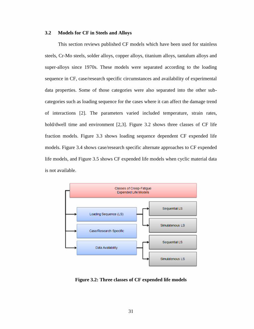
31
3.2 Models for CF in Steels and Alloys
This section reviews published CF models which have been used for stainless
steels, Cr-Mo steels, solder alloys, copper alloys, titanium alloys, tantalum alloys and
super-alloys since 1970s. These models were separated according to the loading
sequence in CF, case/research specific circumstances and availability of experimental
data properties. Some of those categories were also separated into the other sub-
categories such as loading sequence for the cases where it can affect the damage trend
of interactions [2]. The parameters varied included temperature, strain rates,
hold/dwell time and environment [2,3]. Figure 3.2 shows three classes of CF life
fraction models. Figure 3.3 shows loading sequence dependent CF expended life
models. Figure 3.4 shows case/research specific alternate approaches to CF expended
life models, and Figure 3.5 shows CF expended life models when cyclic material data
is not available.
Figure 3.2: Three classes of CF expended life models

32
Figure 3.3: Loading sequence dependent CF
expended life model
Figure 3.4: Case/research specific alternate approaches to
CF expended life models

33
Figure 3.5: CF expended life models when
cyclic material data is not available
Table 3.1: Review of CF assessment methods in literature [6, 8]
Method of life
prediction Life prediction equations
Material parameters needed
(n)
Test
requirements
Linear damage summation
[9]
Strain-life data (4)
Creep-rupture (2-4)
0/0 tests
creep rupture, stress
relaxation
Strain range partitioning
[10] , ij represent PP, PC, CP and CC
loops
Four inelastic strain vs. life relations
(2x4)
Tests producing
complex loops PP,
PC, CP, and CC
Frequency modified
approach [11]
Strain-life data (4)
Frequency vs. life (2)
Stress-strain (2)
0/0 tests, hold time
tests, frequency-life
tests
Damage rate model [12]
Scaling factors (2) 0/0 tests,
metallographic
evidence, hold time
tests
Damage function method
[13]
Strain-life (4) 0/0 data, frequency
data, stress-life data,
hold time data
Damage parameter
approach [14]
Frequency-life (2)
Stress-strain (2)
Shape correction factor
Material parameter (3)
Fatigue damage (2)
Creep damage (2)
Stress versus damage
in creep and fatigue
Viscosity based model
[15]
Total strain and life (2)
Stress-strain (2)
Continuous fatigue

34
3.2.1 Loading Sequence Dependent CF Expended Life Models
In this category, models were separated into two groups of sequential and
simultaneous CF loading. Nearly 90% of the published models are included in the
sequential CF loading category. These life-prediction methods were all at different
stages of development and these models are presented in the following section.
3.2.1.1 Sequential CF Loading
Models presented in this category mostly depend on how cracks behave.They
suffer from crack initiation effects and interaction effects which are unpredictable.
Goswami [6, 8] summarizes empirical life prediction models developed since 1970
and found that only three of those methods received notable interest. They are:
damage summation, strain range partitioning and damage approach [6, 8].
3.2.1.1.1 Linear damage summation
Linear damage summation is widely known as the simplest of the many life-
prediction methods [9, 15]. It is stated as [16]:
(at failure) (3.1)
where and are the fatigue and creep damage ratios, respectively. The
Summation method was employed by the American Society for Mechanical
Engineers in Code Case N-47 [9], and used cycle and time ratios as follows:
(3.2)
where

35
D = total CF damage
n = number of applied cycles at a particular loading condition
= number of cycles to failure at a particular strain range
t = time duration at a particular load condition
= time to rupture from isothermal stress-rupture curves for a given loading
condition
The concept of simply summing creep and fatigue damage has been criticized
for some reasons. The advantages and disadvantages of the cumulative linear damage
summation technique was discussed by Brinkman [15] and a brief summary is shown
below:
1. Compressive and tensile damage are treated equally by using tensile stress-
rupture data for all creep-damage assessment.
2. Some materials such as type 304 stainless steel and alloy 800H show D-values
that are considerably below 1 and tend to decrease with decreasing strain
range and increasing hold time. For typical design situations that involve long
hold periods at low strain rates, it is difficult to justify a given D-value.
3. Environmental interaction, which can influence both crack nucleation and
growth, is not directly accounted for by this method. Therefore, when an
apparent true CF interaction is indicated it actually may be due to
environmental effects.
4. Materials such as 800H, 304 stainless steel or 2-25Cr-1Mo may cyclically
harden or soften, depending on the material, heat treatment and strain range
such that the stress-rupture properties determined from virgin material may
not be appropriate. This problem may be corrected by using cyclic creep data
if available.

36
3.2.1.1.2 Strain range partitioning
In this technique, the inelastic strain range is partitioned into four components:
where the first subscript refers to the tensile and the second to the compressive
deformation [10, 15]. Lifetime relationships for each of these strain ranges are
experimentally established in the form of the Manson-Coffin equation [17]:
(3.3)
where j and k represent p or c. Damage fractions F are usually summed by the
interaction damage rule,
(3.4)
where
and is the inelastic strain range
(3.6)
This method has been used extensively and is one of the easiest to manipulate.
It has had good success in predicting failure of power plant components exposed to
long-term service. It has also been modified to account for mean stress effects and
changes in long-term ductility [15]. However, the disadvantages of this method are
presented as follows:
1. It may be difficult to define the hysteresis loop and accurately partition the
= plastic-plastic = creep-plastic
= plastic-creep = creep-creep
,
(3.5)
,

37
inelastic strain range into the various components, particularly at low strain
ranges
2. The method may be inaccurate in situations where the principal damaging
mechanism is environmental rather than type of deformation.
3.2.1.1.3 Frequency modified approach
This method [18] modifies the original Coffin-Monson and Basquin law
relationships between plastic (inelastic) strain range and cycles to failure with
a frequency factor such that the plastic and elastic components of the total
strain range can be expressed as follows:
(3.7)
(3.8)
where , and are material parameters for a given environment and are
determined by regression analysis of available data [15]. Eq. (3.7) can be expressed
as:
(3.9)
which was further modified to incorporate waveform effects:
(3.10)
where
c = material parameter
= frequency of cycling
= compression-going frequency
= tension-going frequency

38
This method has been used extensively to predict lifetimes for various
materials. It has been criticized [15] for the following reasons:
a) It does not contain a mean stress correction term.
b) With decreasing frequency or increasing duration of a tensile hold time, this
method predicts decreased fatigue life, which doesn’t always occur because of
metallurgical changes as seen in 316 stainless steel.
c) Tensile hold times of equal duration are treated as being equally damaging
irrespective of where they occur in the hysteresis loop, which is not always the
case.
3.2.1.1.4 Damage rate model
This model [19] was developed from observations of the behavior of 304
stainless steel, and assumes that in the low-cycle regime most of the fatigue life is
associated with the growth of cavities and crack growth [15]. It is manipulated on a
differential form of damage with time and employs several equations appropriate for
various waveforms characterizing cavity and crack growth. These growth laws are
integrated over the specimen life, with critical crack and cavity size determined by an
interaction damage rule [15]. However, Brinkman [15] indicates that various
problems have been identified depending on waveform, duration of hold time, and
whether or not a mean stress was present. Crack-nucleation phenomena such as oxide
cracking are ignored. This method needs greater time-dependent fatigue interaction.

39
3.2.1.1.5 Damage function method
Ostergen [19] suggested that the time dependent damage associated with hold
time for a material at a given temperature level can be separated into the two
categories as independent or dependent of waveshape.
a. Time-dependent damage is independent of wave-shape
Ostergen [19] conducted a hold time test on the cast nickel-base “superalloy”
IN738 at 871 . On a uniform gage specimen with axial extensometer and total strain
control, Ostergen defined failure by a change in the character of stress and inelastic
strain, indicative of the presence of a crack of some magnitude.
As far as the method is concerned, since no additional correction for wave
shape beyond using measure of damage appears necessary, this would suggest
a frequency modified failure relation similar to Coffin’s frequency modified equation
[19]:
(3.15)
where
= material constants,
= frequency,
= cycle period,
= time per cycle of continuous cycling,
= tension hold time,
= compression hold time.
When comparable life reduction is dependent only on cycle period, one
would conclude that time-dependent damage is independent of wave shape and that
Eq. (3.15) is the appropriate failure criterion [19]. Further reduction of Eq. (3.15) to
the conventional frequency modified approach is not possible because of the mean

40
stresses which arise from hold times [12]. Additionally, the Coffin-Manson [20]
equation is:
(3.16)
where is the cyclic strain hardening exponent and and are material
constants. For constant strain rate isothermal cycling without hold times, significant
mean stresses do not generally occur [19]. Therefore similar to Eqns (3.15) and
(3.16):
(3.17)
where is the frequency modified stress range and , and are material
constants. For nickel-base superalloy materials (for example, IN738), because
they can be correlated without the frequency term [19]. Therefore, there is very little
time-dependent damage in these alloys.
b. Time dependent damage is dependent on wave shape
Similar to the failure criterion of Eq. (3.15), the failure relation can be written
as:
for
(3.18)

41
for
where
= material constants,
= effective frequency,
= time per cycle of continuous cycling,
= time for which creep occurs in tension (tension hold time), and
= time for which creep occurs in compression (compression hold time).
The effective frequency term , which considers the increase in cycle period by
taking the tensile hold time minus the compressive hold time, is an empirical
approach for including the time-dependent damage of tensile creep and beneficial
effects of compressive creep [12]. The effective frequency is equal to the actual
frequency when hold times occur only in tension; other than it is greater than actual
frequency [19].
3.2.1.1.6 Viscosity based model
Goswami [6] developed a new CF life prediction model with the premise that
deformation under CF test conditions can be represented in terms of viscous behavior,
which is dissipative and irreversible. In an LCF test below (where is melting
temperature of a material in absolute scale), the cyclic damage can be represented by
viscous flow [6]. In modeling steady-state creep behavior, this concept has been
applied. Material parameters used in Goswami’s analysis [6] were analogous to the
dashpot parameters in terms of force and displacement. Steady-state creep behavior is
in terms of linear dashpot process, where velocity is proportional to force. It assumes
constant value of force to give a constant velocity resulting in a linear displacement
versus time behavior. When the force is removed, the motion stops, so that the
deformation is permanent. These concepts were extended in a dwell fatigue situation

42
in which creep and fatigue processes interact. Since these tests are conducted at a
strain level where total strain range exceeds the elastic strain range, the cyclic
deformation is permanent. In order to simulate fatigue,a dynamic velocity term was
used in the model development. It may be noted that fundamental viscosity and
dynamic viscosity concepts are analogous [6]. Goswami [6] presented the dynamic
viscosity as the following Eq.(3.19):
Dynamic viscosity at failure = (3.19)
Since the deformation in a dwell fatigue cycle depends upon the strain range
and time, the rate of damage is in terms of strain rate of a cycle. Therefore, the total
strain range, which has no units, has been multiplied in Eq. (3.19) to account for
strain range effects [6]. The resulting terms has the same units as dynamic viscosity
and is referred to as dynamic viscosity (DV):
DV at failure = (3.20)
When the ability of a material to accommodate viscosity ceases as the dynamic
viscosity reaches a critical value, failure occurs [6]. The ability of a material to
accommodate permanent deformation was assumed in terms of material toughness.
The toughness of a material is a product of ductility and strength:
Material toughness = ductility x strength (3.21)
Since strength in a cyclic fatigue test is in terms of saturated stress range ( )
at a particular strain range, it was used in Eq. (3.21). It may be noted that this stress
value can be determined from actual low cycle fatigue test and depending on cyclic
stress-strain behavior under a particular failure criterion such as 10-50% load drop
43
used in testing. Ductility was determined using drop Edmund and White equation as
follows:
Ductility = (3.22)
Therefore, Eq. (3.22) was substituted in Eq. (3.21) with multiplier giving
material toughness. Therefore, Goswami [6] derives a new CF life prediction
equation by equating these two terms: dynamic viscosity Eq. (3.21) and toughness
Eq. (3.22) and deriving a new life prediction equation as follows:
(3.23)
Since CF life is a dependent on a variety of test parameters [6], Goswami [2]
developed a scaling relationship by plotting strain range vs. strain rate ratios and
cycles to failure on log-log scales. This produced a linear equation with a slope of m
and this slope m was combined with the cyclic stress-strain equation Eq. (3.24) to
develop the following life prediction equation:
(3.24)
An empirical correction factor was used to account for dwell times in the above
equation, which was determined by data fitting as shown below in Eq. (3.25).
Dwell time correction factor =
(3.25)
The dwell time correction factor used in Eq. (3.24) and dwell fatigue life
predicted by the CF data bank, material parameters, e.g., parameters of Coffin-

44
Manson equation, cyclic stress-strain parameters, m and other parameters can be
derived by appropriate data fitting for each material and test.
3.2.1.1.7 Statistical thermal CF models
He [21, 22] investigated the CF behavior of stainless steel materials. He [21,
22] focused on low cycle thermal fatigue life models, and then evaluated statistical
creep models for stainless steel materials. In the low cycle thermal fatigue model, He
[21, 22] used Manson’s universal slopes equation [23], as an empirical relation
relating fatigue endurance to tensile properties. Afterwards, He [21, 22] studied creep
prediction models of Basquin [24] and Sherby-Dorn [24] in order to correlate the
results of short-time elevated temperature tests with long-time service performance at
more moderate temperatures. In this section, the creep prediction models are
evaluated a little bit more in detail, in addition to He’s [21,22] experimental study.
3.2.1.1.7.1 Low cycle thermal fatigue life models
The low cycle thermal fatigue life can be obtained from the total strain range
vs. life curve. When the cyclic material data is insufficient or unavailable, Manson’s
universal slopes equation [23] can be used as an empirical correlation which relates
fatigue endurance to tensile properties:
(3.26)
where is the total strain range, UTS is the ultimate tensile strength, E is the
Young’s modulus, is the number of cycles to failure and is the true ductility
which can be obtained by following equation:

45
(3.27)
where RA is the percentage reduction in area at tensile failure and is the pre-strain
[21, 22].
Table 3.2: Relation between temperature and other parameters [21, 22]
T 450 600 700
Ultimate Tensile Stress, UTS 465 405 326
Elastic Modulus, E 168.5 151 142
% Reudcution in Area, RA (%) 70 70 68
To find the relationship between temperature T and other parameters, He [21,
22] used the data in Table 3.2 in conjunction with different modes. The results
showed that the polynomial model provided the best fit for the relationship
between temperature T and UTS, and a model of the following type was expected:
(3.28)
The natural logarithmic model provided a relative better fit for
the relationship between temperature T and E.
(3.29)
It can be seen from Table 3.2 that for AISI316 stainless steel, % RA only
changes slightly as the temperature increases. Thus, %RA = 70 was used in the study
of He [20, 21]. The true ductility was obtained by following equation:
(3.30)
Substituting Eqns (3.28), (3.29) and (3.30) into Eq. (3.31) gives:

46
(3.31)
Table 3.3: Leading creep rupture models in literature*
Model Trend Eq.
(T in ( in sec)
Material Parameters
needed (n)
REF
Restrained Manson-Brown
(RMB)a
6 Seruga and Nagode
(2011) [25]
Wilshire Equation
3 Wilshire et al. (2009)
[26]
Minimum commitment
6 Manson and Muraldihan
(1983) [27]
Soviet Model 1&2
5 Trunin et al. (1971)
Mendelson-Roberts-Manson
(MRM)a
(n=2,3,4)
min.4-max.6 Mendelson et al. (1965)
[29]
Simplified MRMa (n=2,3,4) min.4-max.6 Mendelson et. al. (1965)
[29]
Orr-Sherby-Dorna log min.4-max.6
Manson-Haferda (n=2,3,4) min.4-max.6 Manson and Haferd
(1953) [29]
Manson-Haferd with
(n=2,3,4) min.4-max.6 Manson and Haferd
(1953) [29]
Larson-Millera (n=2,3,4) min.4-max.6 Larson and Miller, 1952
[29]
a: Models derived from Restrained Manson-Brown
* Adapted from Holdsworth and Daviel [36]
3.2.1.1.7.2 Leading creep rupture models
In order to design reliable systems, accurate information for the elevated-
temperature tensile, creep and rupture test data for stainless steel is required and has
been collected for a number of different steel manufacturers [20, 21]. In this section,
leading creep rupture models as seen in Table 3.3 are discussed.
a. Restrained Manson Brown
The Manson-Brown parameter in particular, given by:

47
(3.34)
is numerically unstable due to the coefficients and q. The set of equations used to
determine the coefficients can be non-linear and cannot be solved trivially. The
restrained Manson-Brown (RMB) parameter is proposed as:
(3.35)
where and q are the coefficients obtained by the least squares method [25].
The value of is if and 0 if . The MB parameter (Eq.(3.34)) is hard to
solve numerically due to the unrestrained coefficients and . Therefore, the RMB
parameter is introduced as a substitute resembling all of the properties of the MB
parameter. This is numerically friendlier to solve because the coefficients can be
determined by solving a set of linear equations and not nonlinear, as in the case of
MB parameter [25]. The states of the RMB parameter represent the Larson-Miller
(LM), Orr-Sherby-Dorn (OSD) and Manson-Haferd (MH) parameter. If , the
RMB parameter represents the MH parameter, given by Eq. (3.34). If , the
RMB parameter represents the OSD parameter, given by:
(3.36)
and if , the RMB parameter represents the LM parameter, given by:
(3.37)
If , 0 or 1, the RMB parameter examines whether or not it is possible to
describe the test data more accurately than with LM, OSD and MH parameters. Every

48
time-temperature parameter is also a function of the stress and this function is usually
a second degree polynomial especially in the case of limited test data [25].
(3.38)
(3.39)
Considering only the RMB parameter (Eq.(3.35)), the relation between the time to
rupture, temperature and stress is thus given by [25]:
(3.40)
This yields Eq. (3.64).
(3.41)
The coefficients and are obtained for the existing creep
rupture test data by the least squares method.
b. Wilshire Equation
It has become common practice to describe creep and creep fracture behavior
in terms of the dependencies of the minimum creep rate and creep life on
stress and temperature using power law expressions of the form [26]:
(3.42)
where R=8.314Jmol-1
K-1
, , the parameter , the stress exponent (n) and
the activation energy for creep are themselves functions of stress and
temperature.

49
In contrast to parametric methods, the stress/creep life plots are easily
superimposed by normalizing the applied stress thorough the measured values of
yield stress or tensile stress . With this approach, is preferred to ,
because property sets can be considered over the full stress range from =1 to
=0 for . Eq. (3.42) can then be re-written as:
(3.43)
where and . Eq. (3.43) avoids the large and variable values
observed using Eq.(3.43), but does not avoid fluctuating n values. In seeking to
quantify creep life behavior over broad stress ranges, must approach zero as
, with points of inflection in the stress rupture plots ensuring that
as [26].
(3.44)
With this relationship, the coefficients are evaluated simply from
plots of ln vs. [26]. However, a distinct change in
and u occurs as decreases. Inserting the derived values of and u into
Eq. (3.44) over the appropriate ranges leads to the sigmoidal ‘master curve’.
Eq. (3.44) provides a clear indication of the high-stress measurements which
should not be included when determining long-term performance [26]. This decision
can be made in an unambiguous manner by discarding results for , but this
approach requires the completion of many long term tests, whereas reasonable
estimates can be produced by applying Eq. (3.44) to data sets with . An
50
additional advantage is then gained by using Eq. (3.44), because no decision is
required on whether the durations of tests which have not failed after long times
should be included when estimating long-term rupture strengths [26].
c. Minimum Commitment
Rupture data were analyzed using Manson’s Minimum Commitment Methods
[27]. All of the data available (264 test results) was used in this analysis by Brinkman
et al. [28]. The Minimum Commitment Method (MCM) equation developed [28] is as
follows:
(3.45)
where all logarithms are base 10.
=rupture life (h)
=stress (MPa)
T=temperature (K)
=867 K
3.2.1.1.7.3 Combining Fatigue and Creep Damages
If there is only one level of fatigue loading and creep loading in the study, the
fatigue damage and creep damage can be identified as follows:
and (3.46)
where represents the number of cycles to failure in continuous fatigue tests, N, is
the number of cycles to failure in CF test, is the rupture time for a pure creep test
and is the hold time [21, 22].
Different damage summation methods were considered by researchers for
comprising both fatigue and creep damage. The linear damage summation rule is still

51
widely used for its simplicity when failure is predicted. Then the linear
damage summation method can be described as follow [21, 22]:
(3.47)
3.2.1.2 Simultaneous CF Loading
3.2.1.2.1 Fii [ ] Model
Holmström and Auerkari [2] proposed a new CF (CF) model based on the
creep rupture behavior of the material with a fatigue correction described by hold
time and total strain range at temperature. This model does not need separation of
creep and fatigue damage or life fractions, and can be applied with a minimum of
input data. The model is shown to predict the observed CF life with a scatter band
close to a factor of 2 for austenitic steel 316FR, ferritic steel P91 and the Ni alloy
A230 [2]. Homlström and Auerkari [2] included only isothermal CF tests under strain
control, with stress ratio R=-1 and hold periods in tension.
The proposed CF model by Holmström and Auerkari [2] aims to predict the
expected life under tensile-compressive loading cycles combined with hold periods of
relaxation. The effective CF lifetime and corresponding number of cycles to
failure are predicted utilizing the creep rupture properties of a material. To
assess CF data, Holmström and Auerkari [2] summed up the hold times for each test
. The proposed Holmström and Auerkari creep rupture model was used to
determine the stress required to produce rupture in this time . This
reference stress was divided with the ultimate tensile strength (UTS) at
temperature to obtain the normalized reference stress (Fii) .

52
Holmström and Auerkari [2] applied the proposed CF approach on the creep
rupture model by Wilshire [26]. Measured values of normalized reference stress
for each point of CF test data can be calculated from:
(3.48)
where k and u are material constants from creep-rupture data, is the apparent
activation energy and R is the gas constant. The required constants are acquired from
fitting with the taken at the same temperature as the creep test
and preferably from the same material batch [2]. The predicted number of cycles to
the “end criterion” is simply calculated as:
(3.49)
To apply this CF model, any other well performing creep rupture models can
be used (see, Table 3.3).
3.2.2 Case/Research Specific Alternate Approaches to CF Expended Life
Models
It was observed that the models in this category are mostly material and path
dependent. Section 3.2.2.1 reviews statistical equations developed for Cr-Mo steels,
stainless steels, generic materials including solder alloys, copper alloys, titanium
alloys and superalloys. Their goodness of fit has been evaluated according to
statistics. is used in the context of statistical models whose main purpose is the
prediction of future outcomes on the basis of other related information. R2 is most
often seen as a number between 0 and 1, used to describe how well a regression line

53
fits a set of data. An R2 near 1 indicates that a regression line fits the data well, while
an R2 close to 0 indicates a regression line does not fit the data very well. It is the
proportion of variability in a data set that is accounted for by the statistical model
[29].
3.2.2.1 Generic Equations
Generic equations [30-33] were originally derived to predict the low-cycle
fatigue response curves of SS304, 316, 321 and recommended in design by American
Society of Mechanical Engineers (ASME). Goswami [6, 8] developed a methodology
to derive a new multi-variate and generic equations according to the coefficient of
correlation value. Furthermore, Goswami [6-8] examined the following alloy
groups and derived a particular model for each case.
a) Cr-Mo steels
b) Stainless steels
c) Generic materials (includes Cr-Mo steels, stainless steels, solder alloys,
copper alloys, titanium alloys, tantalum alloys and superalloys 1782 data
points).
Goswami [6, 8] studied the effect of several variables during testing, whiling
ignoring the effects of composition, microstructure, grain size, heat treatment and
other material parameters to develop general life prediction models. Goswami [6, 8]
utilized only four independent variables as strain range, strain rate, dwell time and
temperature. The transformation functions used were [6, 8].
S = Strain range parameter (S=log( /100))
R = Strain rate parameter (R=log )
T= Temperature parameter (T=T/100) and
H = Hold parameter

54
= % total strain range
= Strain rate (1/s)
= Test temperature
= Predicted cyclic life ( )
= Duration of hold time in hours
The use of transformation functions reduced the scatter in the residual data,
which was the difference between the predicted and observed cyclic life. It is desired
that the data scatters through the scale and does not show the typical trends such as
funnel, double bow and residual non-linear [6-8].
a. Generic Model for Cr-Mo Steels
Goswami [6-8] used a total of 479 data sets for the following low steel alloys:
0.5Cr-Mo, 1Cr-Mo-V, 1.25 Cr-Mo, 2.25Cr-Mo-V and 9Cr-1Mo to derive a
multivariate equation. The dwell times ranged from a few seconds to 48h and the
temperature varied from room temperature to 600 . The total strain range varied
from 0.1% to as high as 2.5% and strain rate, though not specified for each test,
varied from to as low as . The four independent variables
identified earlier were used and a best fit equation was derived for fourth power
optimized for maximum value. It is shown that higher power terms do not
contribute to further improvement in the value. The analysis of variance involved
a corrected total degree of freedom of 473 terms, sum of squares of 13.50, mean
square = 0.14955 and F value of 18.99. A 69-variable, multivariate equation was
developed which gave a value of 76.43%. Thus, 23.57% of the total variations
remain unexplained. This could be due to random samples that were collected, test
run out, premature failures, or to an additional variable, which has not been
considered [6-8].
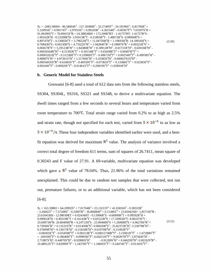
55
Nf = -2081.00004 - 96.58004S2 - 157.18380R2 - 33.27409T2 - 34.18196S3 - 6.81706R3 +
5.12091H3 + 0.99174T3 - 3.97033S4 + 0.09245R4 - 4.36154H4 - 0.00567T4+ 7.03397S2H +
91.06390S2T + 76.69415S3R + 24.38854RH + 173.20087RT - 1.41757HT- 1.41757R2S -
1.90162R3H - 0.23208R4H- 3.91813R3T - 0.21865R4T - 1.48672R3S- 0.08994R4S +
6.89747H2T - 4.13082H3T + 3.79652H4T + 11.04750H2R + 1.19693H4R- 14.18916H2S +
8.76843H3S - 0.04130H4S + 4.71022S2R2 + 1.94284S3R2 + 0.18897S4R2 + 0.09321R3S3 +
0.00457R4S3 + 5.29123R2H2 + 1.84380R3H2 + 0.18912R4H2 - 0.01721R3H4 - 0.02016R4H3 -
0.00026564R4H4 + 4.31392R2T2 + 0.59154R3T2 + 0.03438R3T3 + 0.00497R4T3 +
0.00003261R4T4 - 0.51238H2T2+ 0.33980H3T2 - 0.49672H4T2 + 0.00254H4T4 - 6.49058S2H2 -
0.98987S3H2 + 4.97361S2H3 + 1.21784S3H3 + 0.10385S4H3 - 0.00003761S4H4 -
0.00034935S4R4- 0.61685S2T2 - 0.40559S3T2 - 0.07365S4T2 + 0.13386S3T3 + 0.02383S4T3 -
0.00164S4T4 - 0.00929S3T4 - 0.01461S2T4 + 0.20819S2T3 +1.05891R2H3
(3.50)
b. Generic Model for Stainless Steels
Goswami [6-8] used a total of 612 data sets from the following stainless steels,
SS304, SS304L, SS316, SS321 and SS348, to derive a multivariate equation. The
dwell times ranged from a few seconds to several hours and temperature varied from
room temperature to 700 . Total strain range varied from 0.2% to as high as 2.5%
and strain rate, though not specified for each test, varied from to as low as
. These four independent variables identified earlier were used, and a best-
fit equation was derived for maximum value. The analysis of variance involved a
correct total degree of freedom 611 terms, sum of squares of 26.7411, mean square of
0.30243 and F value of 27.91. A 69-variable, multivariate equation was developed
which gave a value of 78.04%. Thus, 21.96% of the total variations remained
unexplained. This could be due to random test samples that were collected, test run
out, premature failures, or to an additional variable, which has not been considered
[6-8].
Nf = 163.39883 + 64.20992S2 + 7.01704R2 + 25.13215T2 + 41.65816S3 - 0.38332R3
- 3.26665T3 + 7.57208S4 - 0.23007R4 - 36.86686H4 + 0.15386T4 + 23.85942SH + 1.85719S4R -
23.61841RH - 12.08030RT + 0.02434HT - 0.13906R2S - 4.66900R2T + 0.99592R3H +
0.09961R4H + 0.49319R3T + 0.16143R4T + 0.02522R4S + 17.33993H2T- 8.96337H3T -
33.69973H2R- 20.80409H4R + 6.24712H2S - 23.99468H3S + 1.26908H4S + 0.96278S2R2 +
0.73930S3R2 + 0.13531S4R2 + 0.01450R3S3- 0.00620R4S3 - 25.82372R2H2- 5.53079R3H2 -
0.37609R4H2+ 0.13917R3H3 - 0.21810R3H4+ 0.01970R4H3 - 0.31492R2T2
- 0.08381R3T2 - 0.03459R4T2 + 0.00313R4T3- 0.00012748R4T4 - 3.15001H2T2 + 1.67298H3T2
+ .16910H4T2+ 0.18640H2T3 - 0.09993H3T3- 0.04251H4T3 + 0.00287H4T4- 2.87564S2H2 -
2.71987S3H2- 0.44970S4H2 - 8.92880S2H3 - 0.91209S3H3 + 0.04629S4H4- 0.00192S4R4 -
10.48912S2T2- 6.82999S3T2 - 1.24378S4T2 + 1.34692S3T3 + 0.24474S4T3 - 0.01345S4T4 -
(3.51)

56
0.07416S3T4- 0.11433S2T4 + 2.07277S2T3 - 3.72231R2H4
c. Generic Model for High Temperature Materials
Goswami [6-8] used a total of 1782 data sets from the following high
temperature alloys:
a) Solder alloys
b) Copper alloys
c) Steel alloys
1. Cr-Mo low steel alloys
2. Stainless steels
d) Titanium alloys
e) Tantalum alloys
f) Ni-based alloys
Goswami [6-8] varied the dwell times from a few seconds to several hours
and temperature from room temperature to 1100 . In this experimental study [6-8],
the total strain range varied from 0.1% to as high as 5% and strain rate, though not
specified for each test, varied from to as low as . The four
independent variables identified earlier were used and a best fit equation was derived
for fourth power optimized for maximum value. It is shown that higher power
terms do not contribute to further improvement in the value. The analysis of
variance involved a corrected total degree of freedom 1776 terms, sum of squares of
105.53, mean square of 0.82897 and F value of 34.44. A 78-variable, multivariate
equation was developed which produced a value of 61.27%. Thus, 38.73% of the
total variations remained unexplained. This could be due to random test samples that
were collected on so many different materials ranging from solder alloys, test run out,
premature failures, or to an additional variable, which has not been considered.

57
Nf = 0.08317 + 1.09592S2 + 0.28803R2 - 3.92644H2 + 0.11683T2 + 0.12602S3+ 0.08337R3 +
0.48073H3 - 0.02490T3- 0.01410S4 + 0.00427R4 - 0.07199H4 + 0.00136T4 + 0.05327SR - 0.00292S3T +
0.99189RH + 0.00582RT + 0.09628HT + 0.07534R2S + 0.02614R2H - 0.07225R3H - 0.00807R4H +
0.01471R3T + 0.00271R4T+ 0.04763R3S + 0.00489R4S - 0.23417H2T+ 0.15182H3T + 0.03809H4T -
0.78985H2R+ 0.20922H3R - 0.01827H4R - 6.30474H2S + 1.05744H3S + 0.01944H4S - 0.07108S2R2-
0.00131S4R2 - 0.01761R2S3 -0.00089565R3S3 - 0.00019713R4S3+ 0.15444R2H2 + 0.10979R3H2 +
0.01101R4H2 - 0.04600R3H3 + 0.00573R3H4 - 0.00438R4H3 + 0.00052764R4H4 - 0.00126R2T2 -
0.00209R3T2 - 0.00041344R4T2+ 0.00006870R3T3 +0.00002351R4T3- 4.70403E - 7R4T4 +
0.01583H2T2- 0.01689H3T2 - 0.00899H4T2- 0.00059596H2T3 + .00076001H3T3+ 0.00087790H4T3 -
0.00003188H4T4- 3.79717S2H2 - 0.95991S3H2- 0.08619S4H2 + 0.68806S2H3+ 0.17249S3H3 +
0.01406S4H3+ 0.00026628S4H4 - 0.00001764S4R4+ 0.06530S2T2 + 0.05116S3T2+ 0.00915S4T2 -
.00887S3T3- 0.00163S4T3 + 0.00007714S4T4 + 0.00040737S3T4 + 0.00043237S2T4- 0.01039S2T3 -
0.09279R2H3+ 0.01364R2H4
(3.52)
d. Generic Fii [ ] Model
Holmström and Auerkari [2] proposed a new CF (CF) model based on the
creep rupture behavior of the material with a fatigue correction described by hold
time and total strain range at temperature. This model does not need to separate creep
and fatigue damage or life fractions, and can be applied with a minimum of input
data. The model is shown to predict the observed CF life with a scatter band close to a
factor of 2 for austenitic steel 316FR, ferritic steel P91 and the Ni alloy A230 [2].
Homlström and Auerkari [2] included only isothermal CF tests under strain control,
with stress ratio R = -1 and hold periods in tension. The values of from Eq. (3.54)
can then be fitted with multi-linear regression as a function of total strain range ,
hold time and temperature (T) as:
(3.53)
was shown in Eq.(3.55) have a multi-linear relationship in the total strain range,
hold time and temperature against the logarithm of [2].

58
3.2.3 CF expended life models when cyclic material data is not available or not
enough
3.2.3.1 Sequential CF loading
In this category, one model (Statistical thermal CF loading [21]) was included.
Statistical thermal CF loading [21] is presented in subsection 3.2.1.1.7 Statistical
thermal CF models.
3.2.3.2 Simultaneous CF loading
In this category, one model (Fii model [2]) was included. Fii model [2] is
presented in subsection 3.2.1.2.1 Fii Model.
3.2.4 Modified Robust Model(s) for CF
The modifications made are merely for the rupture time variable. As
Holmstörm and Auerkari [2] suggested, any creep rupture model may be of concern
to assess CF life in materials under elevated temperature as long as is
assumed instead of creep rupture time. Also, is assumed to be the maximum
relaxation stress observed in each strain controlled tensile hold CF test data. Among
these models, only Fii model was modified previously by Holmström and Auerkari
[24]. The rest of the models have been converted according to the approach presented
in this publication.
Fii Model [2] (Adapted from Wilshire Equation [26]
(3.54)
Restrained Manson Brown (RMB) [25]

59
(3.55)
Minimum Commitment [Manson and Muraldihan [27]]
(3.56)
Soviet Model 1& 2 (1971)
(3.57)
Mendelson-Roberts-Manson [29]
(n=2,3,4) (3.58)
Simplified MRM [29]
(n=2,3,4) (3.59)
Orr-Sherby Dorn [29]
log (3.60)
Manson-Haferd [29]
(n=2,3,4) (3.61)
Manson-Haferd with [29]
(n=2,3,4) (3.62)
Larson-Miller [29]

60
(n=2,3,4) (3.63)
3.2.4.1 Comparisons of Modified Leading Models
Comparison of the prediction performance for the modified CF models above
has been conducted with the experimental data provided by Holmstrom and Auerkari
[2] for 316FR. Figure 3.6 shows the experimental data used to evaluate the prediction
performance of the well-known creep-rupture models which were converted into CF
life fraction. Figure 3.7 shows for 316FR at 550 C, the R2 statistics for each of the CF
models that were converted into CF life fraction models. It was observed that all the
presented a prediction performance greater than 0.90 R2.
Figure 3.6: Normalized reference stress (Fii) as a function of tCF
for 316FR at 550 [2]

61
Figure 3.7: CF model R2 for 316FR at 550C
Figure 3.8: Generic schematic of strain and
stress history for a fully reversed strain cycle
with hold time at maximum tensile strain

62
3.3 Creep Models in Cyclic Relaxation Response under CF Conditions
It is known that the creep mechanisms of stress relaxation are the main reasons
for fatigue life reduction under CF interactions after a long enough time are the same
as that of long-term monotonic creep. The benefit of this is that a large amount of
creep information can be obtained from a short term relaxation test [34]. Since
relaxation during most of the tests occurred in cyclically hardened materials, it would
have been more appropriate to relate creep damage to stress-rupture curves for
materials that had been cyclically hardened, if such information had been available
[34] (see, Figure 3.8)
To determine the form of the relaxation curve, it is assumed that the total strain
is composed of elastic, plastic and creep components [5]:
(3.65)
Under the tension condition of total strain controlled LCF with hold, the elastic
and plastic strain components remain constant during hold time [4]. Hence
the sum of the each strain rate is given by,
(3.66)
(3.67)
where and represent the elastic and plastic strain respectively. Thus, the time
dependent creep strain rate can be expressed in terms of elastic modulus and a
stress relaxation rate by,
(3.68)

63
where and are the instantaneous relaxation stress and time, respectively and the
value of is negative during stress relaxation. Thus, the plastic strain rate is
determined from the rate of change in stress during stress relaxation, and therefore its
value changes throughout the hold time [4].
By analyzing the value of activation volume for initial transient relaxation
behavior in which the stress is relaxed drastically, it has been suggested that the rate
controlling dislocation mechanisms is either cross slip, or overcoming Peierls-
Nabarro stress [4]. Thus, the temperature dependence of creep rate was identified
during stress relaxation. It was shown that the creep mechanism is identical to steady
state monotonic creep after a long enough hold time which is diffusion controlled
dislocation climb [4].
For most solid materials, it has been shown that the steady state creep rate is
related to the applied stress and temperature by,
(3.69)
where is the apparent activation energy for creep, T is the absolute temperature,
and A and n are the structure factor and the creep exponent, respectively. Therefore,
the stress dependence of the creep rate after transient inelastic behavior due to the
initial loading can be represented by,
(3.70)
So if dislocation creep is considered, the strong dependence of creep rate on
the applied stress is observed. Stress dependence on creep rate can also have a
hyperbolic sine equation form:

64
(3.71)
Nevertheless, these equations model only secondary creep, whereas real creep
curves exhibit a nonlinear (in time) primary creep stage that can be modeled as
follows [5]:
(3.72)
(3.73)
The main difference is that total strain is constant in tensile hold test and the
tensile hold test and the stress is changed with time, whereas the stress is constant in
monotonic creep. Therefore, it may be possible to interpret the stress dependence of
the rate change as a function of the hold time [4].
Applying the linear damage fraction rule to determine the creep damage term
requires numerical integration of stable stress relaxation curves. To simplify the
integration process, relaxation curves were approximated by the function [34]:
(3.74)
or
(3.75)
Best fit values of A and m were obtained by least squares regression of each
stable relaxation curve (see, Figure 3.9).

65
Figure 3.9: Stress relaxation curves at three test temperatures
in a total strain range [4]
3.3.1 Applicable Creep Model(s) in Cyclic Relaxation Response under CF
Conditions
Since hold periods contain only creep deformation, using all the CF hold times
from all of CF cycles to the end criterion, it is possible to look for a creep
deformation curve that covers all three regions in addition to the suggestion provided
by Lafen [5]. Lafen proposed that a creep curve including time dependencies could be
used to predict the primary and secondary regions of the creep curve.
Long-term constant loading at elevated temperatures leads to the
development of creep behavior as a material is damaged and eventually leads to the
failure of engineering structures or components [49]. Creep properties of materials
form the basis to analyze the high- temperature structural strength and life of
materials under constant applied stresses. There exist some creep-damage
equations, such as Kachanov–Rabotnov (K–R) creep-damage formula [50-52],

66
theta projection [53-59] model, and modified Theta-Omega model [52] that
have been widely used to predict the creep damage and the residual strength of
different materials. These models are briefly explained below.
Table 3.4: Published creep models that describe the whole creep curve from
primary (P) to secondary (S) and tertiary part for 10Cr-Mo (9-10) steel alloys
[35-36]
Model Equation Model Creep
Range References
Graham-Walles (1995) Power law P/S/T [37]
Evans and Wilshire Theta
Model (1985) Exponential P/S/T [38]
Modified Theta model
(1985) Power law P/S/T [39]
Kachkanov-Robotnov
(1986) Power law P/S/T [40-43]
Bolton (1994) Power law P/S/T [44-45]
Dyson-McLean (1998) Exponential P/S/T [46]
Modified Garofalo (2001) Exponential P/S/T [47]
Holmström-Auerkari-
Holdsworth (LCSP) Power law P/S/T [48]
Nuhi’s Probabilistic
Model (2011) Power law P/S/T [35]
Kachkanov-Rabotnov (K-R) constitutive [40-43]:
(3.76)
(3.77)
Integration of and substitution in the relation for and further
integration results to the following simplified strain time equation:

67
(3.78)
where and are, respectively equivalent creep strain and stress. is the
maximum principal stress, is the damage variable can be ranged from 0
(no damage) to 1 (full damage ), and and are strain and time to
rupture. The terms D, B, n, , and are material parameters which are
obtained from uniaxial tensile creep curves.
Theta-projection model [39]:
(3.79)
where t is the time, and are parameter constants determined by
fitting the equation to experimental data.
Theta-Omega model [38]:
(3.80)
where X(1), X(2), X(3) and X(4) are parameters constants characterizing
creep curve shapes.
Nuhi’s empirical model [35]:
(3.81)
where a,n,c,m and p are parameter constants describing the creep curve.
Faridani [35] performed an akaike evaluation on the data from experimental and
damage simulation of creep damage for duralumin alloy 2A12, given in the literature
[60], and fitted into all above-mentioned models. The results are given in Table 3.5.

68
Table 3.5: AIC values from comparison of different creep models for the given
experimental data [35]
Empirical –
model Theta – model
Theta – Omega-
model K-R-model
n 39 39 39 39
k 5 4 4 6
AIC -432.3 < -422 < -363 < -357
AIC was computed from the results of least-square estimation or a
likelihood- based analysis. Akaike‘s approach allows identification of the best
model in a group of models and allows ranking the rest of the models easily. The
best model has the smallest AIC value. In Table 3.5, the AIC-values are ranked
in ascending order as follows: Empirical Model, Theta Model, Theta-Omega
Model and the K-R Model respectively, which indicates that the proposed
empirical model is a superior model for describing the creep- damage process. It
should be mentioned that K-R model which has the highest number of parameters
(variables), has the worst ranking.
3.3.2 Comparisons of Modified Robust Models
Comparison of the creep models for steel data in terms of highest goodness of
fit on the was evaluated here once more on the data provided in Figure 3.10. It was
observed that in addition to the model suggested by [5]-[34]. Faridani’s [35]
empirical equation and the modified theta model could be good candidates to predict
the creep deformation behavior in cyclic relaxation response under CF. R2 results can
be seen in Figure 3.10 for 1Cr-Mo-V steel CF data.

69
In addition to CF expended life models, these creep models are validated on
the same experimental CF data.
Figure 3.10: R2 results for creep deformation in stress relaxation
curves at 813 K test temperature in a total strain range
3.4 References
[1] Evans, J.L. and Saxena, A., “Modeling Creep Fatigue,” In. Furrer D.U. and
Semiatin, S.L. (Eds.), ASM Handbook, Vol.22A: Fundamentals of
Modeling for Metals Processing, pp:419-428, 2009
[2] Holmstörm, S. and Auerkari, P., “A robust model for creep-fatigue life
assessment,” Materials Science & Engineering A, Vol. 559, pp.333-335,
2013.
[3] Asayama, T. and Tachibana, Y., “Collect Available Creep-Fatigue Data and
Study Existing Creep-Fatigue Evaluation Procedures for Grade 91 and
Hastelloy XR,” DOE/ASME Generation IV Materials Project, Japan
Atomic Energy Agency, September 30, 2007.
[4] Jeong, C.Y. and Nam, S.W., “Stress dependence on stress relaxation creep
rate during tensile holding under creep-fatigue interaction in 1Cr-Mo-V
steel,” Journal of Materials Science, Vol.34, pp:2513-2517, 1999.
[5] Lafen, J.H. and Jaske, C.E., “Cyclic relaxation response under creep-fatigue
conditions,” Stress Relaxation Testing, ASTM STP 676, pp:182-206, 1976.
[6] Carden, A.E., McEvily, A. and Wells, C.H., Fatigue at elevated

70
temperatures, American Society for Testing and Materials, 1974.
[7] Goswami, T., “Development of generic creep-fatigue life prediction
models,” Materials and Design, Vol.25, pp.277-288, 2004.
[8] Toland, J. and Goswami, T., “General creep-fatigue life prediction models,”
Journal of the Mechanical Behavior of Materials, Vol.15, Issue 1-2, 2004.
[9] Anon. Code Case N-47, ASME boiler and pressure vessel code, “Criteria
for design of elevated temperature,” Class 1 Components in section III,
division 1, American Society of Mechanical Engineers, 1976.
[10] Halford, G.R., Saltsman, J.F. and Hirschberg, M.H., “Ductility normalized
strain range partitioning life relations for creep-fatigue life predictions,”
NASA Report TMX 67838, 1971.
[11] Majumdar, S., Maiya, P.S., “Wave shape effects in elevated temperature
low-cycle fatigue of type 304 stainless steel,” ASME/CSME Pressure Vessel
and Piping Conference, PVP-PB 028, 1978.
[12] Maiya, P.S., “Effects of wave shape and ultrahigh vacuum on elevated
temperature low cycle fatigue in type 304 stainless steel,” Material Science
and Engineering, Vol.47, pp.13-21, 1981.
[13] Chrzanowski, M., “Use of the damage concept in describing creep-fatigue
interaction under prescribed stress,” International Journal of Material
Sciences, Vol.18, Issue 2, pp.69-73, 1976.
[14] Goswami, T., “Low-cycle fatigue life prediction - a new model,”
International Journal of Fatigue, Vol. 19, Issue 2, pp:109-115, 1997.
[15] Brinkman, C.R., “High temperature time-dependent fatigue behavior of
several engineering structural alloys,” International Metal Reviews, Vol.30,
Issue 5, pp:235-258, 1985.
[16] Coffin, L.F., “”Methods for predicting life in fatigue,” American Society of
Mechanical Engineers, pp:1-24, New York, 1979.
[17] Manson, S.S., Halford, G.R. and Hirschberg, M.H., “Creep-fatigue analysis
by strain-range partitioning,” 1st National Pressure Vessel and Piping
Conference Sponsored by the American Society of Mechanical Engineers,
pp: 12-24, New York, 1971.
[18] Coffin, L.F., “Fatigue at high temperature – prediction and interpretation,”
Inst MechEng, Vol.188 9, Issue 74, pp.109-127, 1974.

71
[19] Ostergren, W.J., “A damage function and association failure equations for
predicting hold time and frequency effects in elevated temperature, low
cycle fatigue,” Journal of Testing and Evaluation, Vol.4, Issue 5, pp. 327-
339, 1976.
[20] Manson, S.S., Thermal stress and low cycle fatigue, McGraw-Hill, p:171,
New York, 1966.
[21] He, X., “Statistical thermal fatigue-creep modeling of stainless steel
materials,” IEEE, 2009.
[22] He, X., Li, G. and Ding, Y., “Statistical thermal creep-fatigue modeling of
316 stainless steel materials,” Scientific Research Essays, Vol.6, Issue 20,
pp:7172-7178, 19 September, 2011.
[23] Manson, S.S., “A complex subject – some simple approximations,”
Experimental Mechanics, Vol.5, Issue 7, pp:193-326, 1965.
[24] Truman, R.S. et al., “Elevated-temperature tensile, creep and rupture
properties of 18%Cr-8%Ni, 18%Cr-12%Ni-Mo, 18%Cr-10%Ni-Ti, and
18%Cr12%Ni-Nb steels,” Proceedings of Joint Conference Organizaed by
the British Iron and Steel Research Association and the Iron and Steel
Institute, pp:265-300, Eastbourne, UK, 1966.
[25] Seruga, D. and Nagude, M., “Uniform of the most commonly used time-
temperature creep parameters,” Material Science
and Engineering A, Vol.528, pp:2804-2811, 2011.
[26] Wilshire, B., Scharming, P.J. and Hurst, R., “A new approach to creep data
assessment,” Material Science and Engineering A, Vol.510-511, pp:3-6, 15
June 2009.
[27] Manson, S.S. and Muralidharan, U., “Analysis of creep-rupture data for five
multi-heat alloys by the minimum commitment method using double heat
term centering,” Progress in Analysis of Fatigue and Stress Rupture MPC-
23, ASME, pp:43-60, 1984.
[28] Brinkman, C.R., Booker, M.K. and Ding, J.L., “Creep and creep-rupture
behavior of Alloy 718,” Special Emphasis Symposium on Superalloys 718,
625, and Various Derivatives, Pittsburg, PA (USA), 23-26 Jun 1991.
[29] Steel, R. G. D. and Torrie, J. H., Principles and Procedures of Statistics,
New York: McGraw-Hill, pp:187-287, 1960.
[30] Diercks, D.R. and Raske, D.T., “A statistical analysis of elevated

72
temperature, strain controlled fatigue data on type 304 stainless steel,”
ASME Annual Winter Meeting, New York, December 5-10, 1976.
[31] Sonoya, K., Nonaka, I. and Kitagawa, M., “Prediction of creep-fatigue lives
of Cr-Mo steels with Direcks Eq.,” ISIJ International, Vol. 1, No.12,
pp.1424-1430, 1991.
[32] Langer, B.F., “Design of pressure vessels for low-cycle fatigue,” J Basic
Eng, Vol.84, Issue 3, pp.389-402, 1962.
[33] Goswami, T., “Creep-fatigue life prediction of Cr-Mo steel alloys,” In.
Laiw, P.K., Bunchanan, R.A., Klarstrom, D.L., Wei, R.P., Harlow, D.G.,
Tortorelli, P.F. (Eds.), Material lifetime science and engineering, pp.43-50,
2003.
[34] Jaske, C.E., Mindlin, H., and Perrin, J.S., “Combined Low-Cycle Fatigue
and Stress Relaxation of Alloy 800 and Type 304 Stainless Steel at Elevated
Temperatures, ”Fatigue at Elevated Temperature, ASTM STP 520,
American Society for Testing Materials, pp:365-376, 1973.
[35] Faridani, M.N. and Modarres, M., “Classification and probabilistic model
development for creep failures of structures: study of X-70 carbon steel and
7075-T6 aluminum alloys,” Thesis, In partial fulfillment of the
requirements of the degree of Master of Science, Fall 2011.
[36] Holdsworth, S.R., Merckling, G., “ECCC developments in the assessment
of creep rupture data,” In: Proceedings of sixth international Charles
Parsons Conference on engineering issues in turbine machinery, power
plant and renewable, Trinity College Dublin, 16-18 September, 2003.
[37] Graham, A. and Walles, K.F.A. ; NGTE Reports Nos.R.100(1952), R.137
(1953), R.189 and R.190 (1956); J. Iron and steel Inst.179,105, 1955.
[38] Moles, M. D. C. and Westwood, H. J.; “ Residual life estimation of high
temperature superheater and reheater tubing, CER RP, 78-66, Final report
of Ontario Hydor Research Dev., Toronto, for the Canadian Electrical
Assn., Montreal, pp: 67-82, Mar. 1982.
[39] Johnson, G.R.; Cook, W.H., "A constitutive model and data for metals
subjected to large strains, high strain rates and high", 1983.
[40] Johnson,G. R.,Cook, W.H. ; Fracture characteristics of three metals
subjected to various strain rates, temperatures and pressures, Eng.
Fracture Mechanics, Vol.21, Issue:1, pp:31-48, 1985.
[41] Modified Theta model in: R.W. Evans and B. Wilshire, Creep of

73
metals and alloys, Institute of Metals, 1985.
[42] Rabotnov, Y.N. ; Some problems of the theory of creep, NACA., TM, 1353,
1953.
[43] Rabotnov, Y. N. ; On the equation of state of creep, ASME/ASTM/IMechE
Proceedings Conference on creep, Inst. Mech. E., New York/London,
1963.
[44] Maruyama, K. et al. ; Long-term creep curve prediction based on the
modified θ projection concept. J. Pressure Vessel Technol., 112, 1990.
[45] Brinkman, C.R.; Booker, M.K.; and Ding, J.L.: Creep and Creep-Rupture
Behavior of Alloy 718. Proceedings of the International Symposium on
the Metallurgy and Applications of Superalloys 718, 625, and Various
Derivatives, Minerals, Metals & Materials Society, Warrendale, PA,
1991.
[46] Prager, M. 'Development of the MPC Omega method for life
assessment in the creep range', ASME J. Pressure Vessel
Technology, 117, May, 95-103, 1995.
[47] BJF-model: Jones, D.I.G, French, R.M. and Bagley, R.L.; A Renewal
Theory of Inelastic Thermo-Mechanical Behavior of Metal Alloys‖; ASME
AD-Vol. 50, Fatigue and Fracture at Elevated Temperatures, A. Nagar and
S. Mall, ed.; Book No. H01013 1995.
[48] Baker and Cane model: Baker AJ, O‘Donnell MP. R5 high temperature
structural integrity assessment of a cracked dissimilar metal weld vessel
test. In: Proceedings of second international conference on integrity of
high temperature welds, London, 10–12 November 2003.
[49] Zhao, Bin, et.al., “Experiment and simulation of creep damage for
duralumin alloy” 2A12, Material Science and Engineering A 513-514, 91-
95, 2009.
[50] Lin, J., Kowalewski, Z. L. and Cao, J., Int. J. Mech. Sci. 47, pp. 1038–
1058, 2005.
[51] Kachanov, L. M., Izv. AN SSSR, OTN 8, pp. 26–31, 1958.
[52] Kachanov, L. M., The Theory of Creep, British Library, Boston Sp,
Wetnerley, 1960.

74
[53] Rabotnov, Y. N., Creep Problems in Structural Members, Amsterdam,
North-Holland 1969.
[54] Huang, R., Turbine Technol. 43, pp: 9–13, 2001.
[55] Evans, R.W., and Wilshire, B. “Creep of Metals and Alloys”, The
Institute of Metals, London, 1985.
[56] Evans, R. W. and Wilshire, B., Introduction to Creep, The Institute of
Materials, London 1993.
[57] Burt, H. and Wilshire, B., Metall. Mater. Trans. A 35A, pp. 1691–1701,
2004.
[58] Burt, H. and Wilshire, B., Metall. Mater. Trans. A 36A (2005), pp. 1219–
1227, 2005.
[59] Zhao, Bin., et.al., ”Experiment and simulation of creep damage for
duralumin alloy” 2A12, Materials Science and Engineering A 513-514, 91-
96, 2009.
[60] Ling, X., Zheng. Y. Y. and You, Y. J., Int. J. Pressure Vessels Piping 84
(2007), pp:304-309, 2007.

75
Chapter 4: Experimental Details
4.1 Introduction
In this chapter the experimental procedure conducted in this thesis study is
presented. In progress of this study, initial effort was spent to characterize the
material to be tested. In section 4.2.1, a brief discussion about the test material is
presented with related characterization results.
After material characterization was completed, a uni-axial tensile test was
conducted. A considerable attention was focused on preparation of the required
experimental setup for 1D uni-axial creep-fatigue (CF) test. Temperature is known as
one of the most effective stress parameter for both creep and CF damage [1]. In order
to ensure a reliable test sample temperature measurement, a particular thermocouple
clip was designed.
Eventually, a CF test plan was drafted according to the creep-life prediction
formulas from Larson-Miller [2] and Wilshire [3]. The details of the test specifics
associated with each CF tests are provided at the end this section. A rationale for
selection of CF parameters is presented, and results obtained in the end of each CF
tests were provided.
4.2 Experimental Details
A uni-axial MTS 810 test system machine, which is available in MEMIL
(Modern Engineering Materials Instructional Laboratory) in H. Kim Engineering
Building at UMD, was used to perform uni-axial tensile tests. The test specimen was
a round-bar dog-bone based on ASTM E8/E8M-11 (see, Figure 4.1 and Figure 4.2)
76
[4]. The ASTM standards used to determine the test specimen and test procedure are
listed in Table 4.1.
Figure 4.1: Dimensions by ASTM E8/E8M-11
Table 4.1: Standards used for specimen design and parameters of experimental
tests
Design/Test Standard Definition
Dog-Bone
Specimen E8/E8M-11 [4]
Standard Test Methods for Tension
Testing of Metallic Materials
Tension Test E8/E8M-11 [4] Standard Test Methods for Tension
Testing of Metallic Materials
CF E2714-09e1 [5] Standard Test Method for CF Testing
Since the designed samples were smaller than the typical dimenions used in the
MTS 810, 316 Stainless Steel fixtures were designed as mechanical support. The top
ends of the test samples were threaded in order to allow mounting of the testing
samples into these 316 Stainless Steel fixtures. (see Figures 4.2 and 4.3). Copper coils
were wrapped around these 316 Stainless Steel fixtures to water-cool and to prevent
the heat transfer from the test sample to hydrolic wedge grips of MTS 810 machine
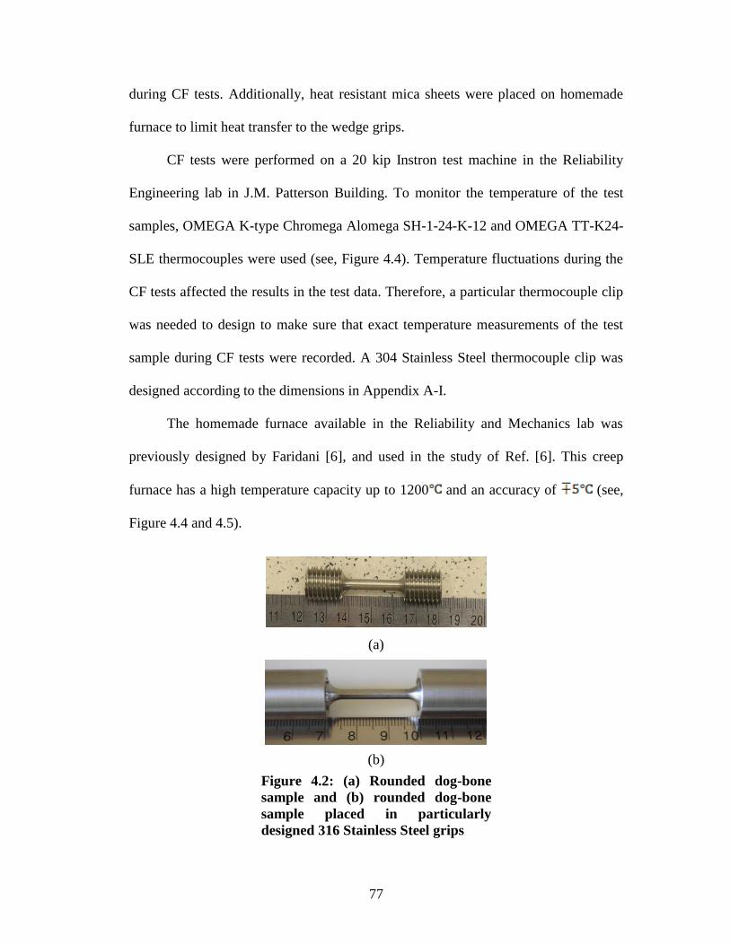
77
during CF tests. Additionally, heat resistant mica sheets were placed on homemade
furnace to limit heat transfer to the wedge grips.
CF tests were performed on a 20 kip Instron test machine in the Reliability
Engineering lab in J.M. Patterson Building. To monitor the temperature of the test
samples, OMEGA K-type Chromega Alomega SH-1-24-K-12 and OMEGA TT-K24-
SLE thermocouples were used (see, Figure 4.4). Temperature fluctuations during the
CF tests affected the results in the test data. Therefore, a particular thermocouple clip
was needed to design to make sure that exact temperature measurements of the test
sample during CF tests were recorded. A 304 Stainless Steel thermocouple clip was
designed according to the dimensions in Appendix A-I.
The homemade furnace available in the Reliability and Mechanics lab was
previously designed by Faridani [6], and used in the study of Ref. [6]. This creep
furnace has a high temperature capacity up to 1200 and an accuracy of (see,
Figure 4.4 and 4.5).
(a)
(b)
Figure 4.2: (a) Rounded dog-bone
sample and (b) rounded dog-bone
sample placed in particularly
designed 316 Stainless Steel grips

78
(a) (b)
Figure 4.3: (a) Designed 316 Stainless Steel
fixtures for rounded dog-bone samples; (b)
A view from tension testing of a rounded
dog-bone sample which is fixed on 647
Hydraulic Grips together with the
particularly designed 316 Stainless Steels
(c)
(a) (b)
Figure 4.4: Creep furnace setup with (a) thermocouples, and (b) copper coil
coolers; (c) 316 Stainless Steel thermocouple clip attached to test specimen inside
the creep furnace

79
Figure 4.5: Power supply unit of home-made creep furnace used to control the
furnace temperature
4.2.1 Material
Energy-dispersive X-ray spectroscopy (EDS) for compositional analysis was
performed on the test material steel alloy using Hitachi SEM-70 in NISP Lab at
UMD. Consequently, a uni-axial tensile test was performed using the MTS 810 in the
MEMIL lab at UMD.
Next, both tested and untested samples were characterized using Scanning
Electron Microscopy (SEM: Hitachi, SU-70) and Atomic Force Microscopy (AFM:
Vecco, D-3000). In order to prepare the untested 7x7mm metal piece of steel alloy
material for SEM analysis, it was first encapsulated in epoxy mixture (see, Figure 4.7
and Appendix B-I). After the encapsulation, the metal piece was polished using
silicon carbide electro coated water proof abrasive papers of CC-23 P600, P1000 and
P1500 respectively under water lubricant to provide a mirror-like quality on the metal

80
piece (see Figures 4.6 and 4.7). The encapsulated metal was analyzed using FEG-
SEM (Hitachi, SU-70). The results of the EDS analysis are presented in Table 4.2.
AFM and SEM pictures of the raw metal surface are provided in Figure 4.8.
Figure 4.9 shows elements dispersion on fractured surface of the tested material after
tension test. This figure also helps us to understand influential elements on the test
material.
Figure 4.6: Automated polishing to provide a
mirror-like quality on encapsulated metal pieces
Figure 4.7: Encapsulated 7 x 7 mm metal piece
for EDS analysis after polishing
Table 4.2: EDS chemical composition results (wt.%)
C Al P S Ti Cr Mn Fe Co Ni Cu Nb
0.66 0.10 0.01 0.14 0.35 16.77 1.83 70.83 0.09 7.44 1.21 0.57

81
(a) (b)
Figure 4.8: (a) AFM picture of raw material surface in nanometer scale, (b)
SEM picture (1000x) of raw material surface in micrometer scale
(a) (b)
Figure 4.9: (a) Fractured tensile specimen, (b) Dispersion of the elements on the
fractured sample surface under SEM microscope
In order to study the general microstructure of steel alloy samples, samples
were etched first using an etchant based on ASTM E407-07 [7]. The chemical
composition preferred was 10mL HNO3, 20-50mL HCl and 30mL water with respect
to the chemical composition results obtained from SEM analysis. The encapsulated
metal was immersed into this etchant solution for times varying from 5min to 15min
to observe the surface topography and general structure (see, Figure 4.10). It was
observed that the applied etchant solution on the polished material did not provide a
sufficient view for general structure investigation.

82
(a) (b)
Figure 4.10: (a) SEM picture for surface topography of 5min immersed metal, and (b)
SEM picture of 15min immersed metal
4.2.2 Tensile Test
A uni-axial tensile test based on ASTM E8/E8M-11 [4] was performed (see,
Figure 4.13). Regarding elongations greater than 5%, suggested range is indicated as
0.05 and 0.5 [mm/mm/min] by the ASTM E8/E8M-11 standard [4]. Hence, 16 mm
gage length of the test sample enabled 0.8 [mm/min] displacement rate. Test inputs
for the MTS 810 software are shown in Figure 4.11. Room temperature tension test
result for the steel alloy is presented in Figure 4.12. Yield strength was defined as
261.3 MPa, and tensile strength was defined as 691.5 MPa. The sample surface
featuring a ductile cup and cone fracture is shown in Figure 4.13-b and Figure 4.14-a.
SEM pictures of the fracture surface at 35x and ruptured surface pores of metal
dog-bone sample at 1000x are shown in Figure 4.14-a and b. It is also observed that
most of the pores were located in the center of the ruptured sample surface.

83
Figure 4.11: MTS 810 test machine software and tension test inputs
Figure 4.12: Tension test result in room temperature for the steel alloy

84
(a) (b)
Figure 4.13: (a) Ruptured dog-bone sample and (b) ductile
cup and cone form of ruptured cross section of the steel
alloy
(a) (b)
Figure 4.14: SEM pictures of the fracture surface of the uni-axial tensile test
sample (a) at 35x and (b) at 1000x showing the presence of surface pores
4.2.3 1D Uniaxial CF Test
Depending on the component type and the purpose of the analysis, a defect-
free or defect assessment procedure (or both) is undertaken to assess fitness for
service at high temperatures [9]. Defect-free assessment procedures are commonly
used for design purposes whereas defect assessment procedures are used for

85
inspection management and remaining life evaluations [8]. Data sets may be a result
of (a) concurrent or (b) sequential CF loading campaigns [8]. The focus of this thesis
study is on the data requirements for defect assessment of high temperature
components which can be determined from CF tests. The data used in this study was
the result of concurrent CF loading.
In this study, CF deformation was evaluated as non-separated regarding the
study of Holmstrom et al. [9]. Holmstrom et al. [9] proposed a robust model for CF
expended life assessment with a minimal set of fitting constants, and without the need
to separate CF or expended life fractions. The CF damage is evaluated simply with
DCF = where is the corresponding time in hold.
According to ASTM E2714-09e1 [5], the preferred cycle shape in this study
was a cycle with a hold at peak of the control parameter in tension (see, Figure 4.15-
a). During the tests performed in this work, no compressive loads were applied
because of the small cross-sectional diameter (4mm) of the samples. ASTM standard
E606/E606M-12 for Standard Test Method for Strain-Controlled Fatigue Testing [10]
recommends the cross-section dimension to be at least 6.35 mm (0.25 in.). Therefore,
to prevent any potential buckling failure during CF test, compressive stresses were
not applied on the test sample. The applied cycle shape which was modified from
ASTM standard E2714-09e1[5] is demonstrated in Figure 4.15-b.
Isothermal CF tests were under strain control with tensile hold periods. Tests
were performed at a stress ratio R = 0 and a fixed temperature at 400 (673.15 ).
Additionally, before any CF tests were performed, calibration of the entire
temperature measurement and control system were performed and it was found that

86
temperatures stayed within of the setpoint. In Figure 4.16, a view from creep-
fatigue test set-up in Reliability and Mechanics lab was demonstrated.
(a) (b)
Figure 4.15: (a) ASTM E2714-09 CF cycle shape: is a cycle with a hold at peak of
the control parameter in tension [5]; (b) Adjusted CF cycle shape according to the
available dog-bone sample design
Figure 4.16: CF test setting in Reliability and Mechanics lab
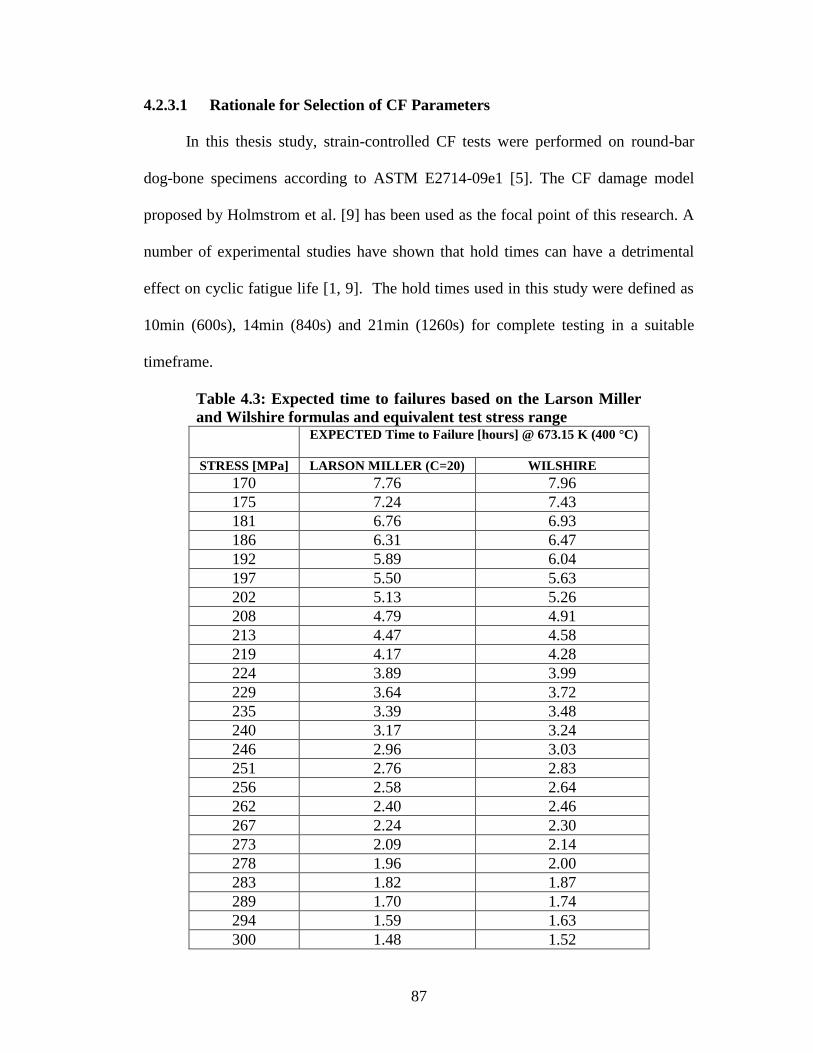
87
4.2.3.1 Rationale for Selection of CF Parameters
In this thesis study, strain-controlled CF tests were performed on round-bar
dog-bone specimens according to ASTM E2714-09e1 [5]. The CF damage model
proposed by Holmstrom et al. [9] has been used as the focal point of this research. A
number of experimental studies have shown that hold times can have a detrimental
effect on cyclic fatigue life [1, 9]. The hold times used in this study were defined as
10min (600s), 14min (840s) and 21min (1260s) for complete testing in a suitable
timeframe.
Table 4.3: Expected time to failures based on the Larson Miller
and Wilshire formulas and equivalent test stress range EXPECTED Time to Failure [hours] @ 673.15 K (400 °C)
STRESS [MPa] LARSON MILLER (C=20) WILSHIRE
170 7.76 7.96
175 7.24 7.43
181 6.76 6.93
186 6.31 6.47
192 5.89 6.04
197 5.50 5.63
202 5.13 5.26
208 4.79 4.91
213 4.47 4.58
219 4.17 4.28
224 3.89 3.99
229 3.64 3.72
235 3.39 3.48
240 3.17 3.24
246 2.96 3.03
251 2.76 2.83
256 2.58 2.64
262 2.40 2.46
267 2.24 2.30
273 2.09 2.14
278 1.96 2.00
283 1.82 1.87
289 1.70 1.74
294 1.59 1.63
300 1.48 1.52

88
Based on the stress-strain curve in Figure 4.12, the displacement amplitude was
set to 0.24mm to prevent any potential premature failure in CF tests. It is suggested
by Ref. [11] that at a temperature beyond 30% of the absolute melting temperature of
the material, significant time-dependent damage is accumulated. Since 30% of the
absolute melting temperature of steel alloys is nearly equivalent to 400 (673.15 ),
the test temperature was decided to keep fixed at this level. This test temperature
level was also preferred in order to prevent any heat-related damage on the test
equipment that might occur at higher temperatures. Rump up and rump down times
were set to 180s which makes a strain rate at 0.005 mm/mm/min. Table 4.3 provides a
summary of the predicted time to failure based on the Larson-Miller [2] or Wilshire
[3] models. These results were derived from the initially performed CF test results at
10min (600s) hold time.
Defined strain amplitude takes into account the coefficient thermal expansion
of the material at 400 C(673.15 ). However, the contribution which came from the
thermal expansion theory was considerably small, and did not affect the results. The
details of the thermal expansion of the test material at 400 C(673.15 ) are explained
in following discussion.
The length increment is linearly proportional to temperature given as [12]:
(4.1)
(4.2)
: change in length (m, inches)
: initial length (m, inches)
: linear expansion coefficient (m/m , in/in )
: change in temperature ( )
: initial temperature ( )
: final temperature ( )
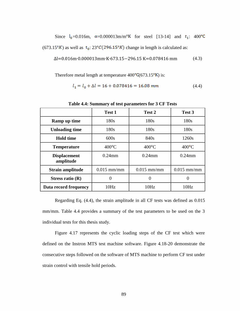
89
Since =0.016m, =0.000013m/m for steel [13-14] and : 400
(673.15 ) as well as : 23 change in length is calculated as:
∆l=0.016m∙0.000013mm∙K∙673.15−296.15 K=0.078416 mm (4.3)
Therefore metal length at temperature 400 (673.15 ) is:
(4.4)
Table 4.4: Summary of test parameters for 3 CF Tests
Test 1 Test 2 Test 3
Ramp up time 180s 180s 180s
Unloading time 180s 180s 180s
Hold time 600s 840s 1260s
Temperature 400 C 400 C 400 C
Displacement
amplitude
0.24mm 0.24mm 0.24mm
Strain amplitude 0.015 mm/mm 0.015 mm/mm 0.015 mm/mm
Stress ratio (R) 0 0 0
Data record frequency 10Hz 10Hz 10Hz
Regarding Eq. (4.4), the strain amplitude in all CF tests was defined as 0.015
mm/mm. Table 4.4 provides a summary of the test parameters to be used on the 3
individual tests for this thesis study.
Figure 4.17 represents the cyclic loading steps of the CF test which were
defined on the Instron MTS test machine software. Figure 4.18-20 demonstrate the
consecutive steps followed on the software of MTS machine to perform CF test under
strain control with tensile hold periods.

90
The print-screen in Figure 4.18 demonstrates the inputs provided in first step.
In this demo test, step1 in Figure 4.18 was completed in 30s, and ramped up to the
specified displacement position according to the Instron MTS coordinate system.
Figure 4.19 demonstrates the inputs in the second step of the cycle presented in
Figure 4.17. Figure 4.20 shows the third step of the cycle presented in Figure 4.17.
Rump down duration was set equal to the rump up duration. The end point was
specified as the defined end point in the step 1 minus specified displacement level.
Figure 4.21 presents the instant test monitor module. In this module, triple
chart display option was selected. The display graphs were defined to monitor
instantly stress-time, strain-time and stress-strain hysteresis diagrams.
Figure 4.17: Strain controlled CF test cycle with
stress Ratio = 0, where Step1(Tension), Step 2(hold)
and Step 3(release)
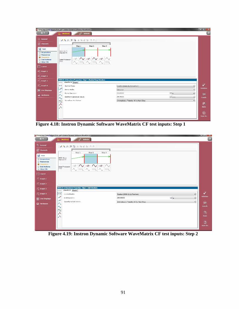
91
Figure 4.18: Instron Dynamic Software WaveMatrix CF test inputs: Step 1
Figure 4.19: Instron Dynamic Software WaveMatrix CF test inputs: Step 2

92
Figure 4.20: Instron Dynamic Software WaveMatrix CF test inputs: Step 3
Figure 4.21: Instron Dynamic Software WaveMatrix test monitoring options
ASTM standard E2714-09e1 [5] defines the failure criteria for CF tests when at
least a 10% reduction in the stress with respect to the maximum load is observed (as
seen in Figure 4.22 where x = 10%). Therefore, the failure criterion in each CF test

93
used in this study was initially defined according to the observed stress reduction with
respect to the observed maximum reference stress during the test. It was observed that
nearly after 60% drop with respect to the reference (stress) level, instant on the
same CF test reached to zero level.
Figure 4.22: ASTM standard E2714-09 end-
of-test criterion based on reduction of peak
stress for softening materials
4.2.3.2 1D Uniaxial CF Test Results
Figure 4.23 provides stress-strain hysteresis diagram for a 10min (600s) hold
time strain controlled creep-fatigue test at 673.15 . Due to the short hold
time of the test, it is difficult to observe any certain reduction of stress in each
hysteresis cycle at the strain control point of 0.015 mm/mm. The expected reduction
of stress is shown in the red circle for a definite hysteresis cycle (see, Figure 4.23).
Figure 4.24 demonstrates strain – cycles to failure graph for 10min (600s) hold
time CF test at 0.015 [mm/mm]. Strain amplitude can be seen easily in this figure.
Figure 4.25 provides a stress-cycle to failure graph for the 10min (600s) hold
time test at . After 41 cycles, a 58% drop in the stress with respect
to the initial reference stress was observed. In the subsequent cycle, a sudden drop to
zero stress level was observed.

94
Figure 4.23: Stress-strain hysteresis diagram for all cycles in 10min (600s)
hold time creep CF test at 673.15
Figure 4.24: Strain-cycle to failure diagram for all cycles in 10min(600s) hold
time CF test at 673.15

95
Figure 4.25: Stress-cycle to failure diagram for all cycles in 10min (600s) hold
time CF test in 673.15
In Figure 4.26, strain – cycle to failure graph of 14min (840s) hold time creep-
fatigue test is provided. Strain control in 0.015 [mm/mm] was maintained throughout
the all cycles in this test.
Figure 4.26: Strain-cycle to failure diagram for all cycles in 14min (840s) hold
time CF test at 673.15
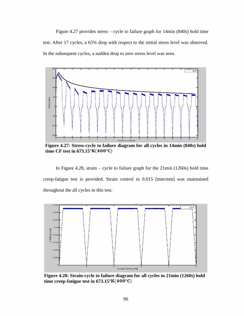
96
Figure 4.27 provides stress – cycle to failure graph for 14min (840s) hold time
test. After 17 cycles, a 65% drop with respect to the initial stress level was observed.
In the subsequent cycles, a sudden drop to zero stress level was seen.
Figure 4.27: Stress-cycle to failure diagram for all cycles in 14min (840s) hold
time CF test in 673.15
In Figure 4.28, strain – cycle to failure graph for the 21min (1260s) hold time
creep-fatigue test is provided. Strain control in 0.015 [mm/mm] was maintained
throughout the all cycles in this test.
Figure 4.28: Strain-cycle to failure diagram for all cycles in 21min (1260s) hold
time creep-fatigue test in 673.15

97
Figure 4.29 provides stress – cycle to failure graph for 21min (1260s) hold time test.
After 5 cycles, 100% drop with respect to the initial stress level was observed.
Figure 4.29: Stress-cycle to failure diagram for all cycles in 21min (1260s) hold
time CF test in 673.15
Figure 4.30 illustrates the striated surface of visually deformed test sample
after CF test. The actual observations were akin to this illustration.
Figure 4.30: Test sample before and after CF
test showing the visual impact of CF
deformation on the sample surface
Figure 4.31 illustrates the observed stress levels in each creep- fatigue test with
respect to the stress – strain curve of the material in room temperature. Figure 4.32

98
shows the number of cycles to failure with respect to different hold times for the
different creep-fatigue tests. It was observed that as hold time increases the time to
failure decreases.
Figure 4.31: Observed stress levels in each CF test with respect to the
stress-strain curve in room temperature
Figure 4.32: Observed number of cycles to failure with respect to the
hold times in each CF test
4.3 References
[1] Brinkman, C.R., “High-temperature time-dependent behavior of several
engineering structural alloys,” International Metal Reviews, Vol.30, Issue:5,

99
pp:235-258, 1985.
[2] Larson, F.R., Miller, E.J., “Time-temperature relationship for rupture and
creep stresses,” Trans. ASME, vol.74, p.765-775, 1952.
[3] Wilshire, B., Scharning, P.J., Hurst, R., “A new approach to creep data
assessment,” Materials Science and Engineering A, Vol.510-511, Issue:3-6,
2009.
[4] ASTM Standard E8/E8M-11, “Standard test methods for tension testing on
metallic materials,” ASTM International, West Conshohocken, PA, 2011,
DOI:10.1520/E0008_E0008M-11, www.astm.org.
[5] ASTM Standard E2714-09e1, “Standard test method for creep-fatigue
testing,” ASTM International, West Conshohocken, PA, 2009, DOI:
10.1520/E2714-09EOI,www.astm.org
[6] Faridani, M.N, and Modarres, M., “A probabilistic model of creep failure
mechanism for structural reliability assessment with applications,” 2012.
[7] ASTM Standard E407-07, “Standard practice for microetching and alloys,”
ASTM International, West Conshohocken, PA, 2007, DOI: 10.1520/E0407-
07, www.astm.org.
[8] Holdsworth, S.R., “Component Assessment Data Requirements from Creep-
Fatigue Tests,” Journal of ASTM International, 2011, www.astm.org.
[9] Holmstrom, S., Auerkari, P, “A robust model for creep-fatigue life
assessment,” Material Science and Engineering A, vol.559, pp: 333-335,
2013.
[10] ASTM Standard E606/E606M, “Standard Test Method for Strain-
Controlled Fatigue Testing,” ASTM International, West Conshohcken, PA,
2012, DOI: 10.1520/E0606-04E01, www.astm.org .
[11] Mao, H., Mahadevan, S., “Reliability analysis of creep-fatigue failure,”
International Jornal of Fatigue, Vol.22, pp:789-797, 2000.
[12] Jaske, C.E., Mindlin, H and Perrin, J.S., “Combined low-cycle fatigue and
stress relaxation of alloy 800 and type 304 stainless steel at elevated
temperatures,” Fatigue at elevated temperature, ASTM STP 520, American
Society for Testing and Materials, pp:365-376, 1973.
[13] Sun, G., Chen, Z., Liu, Z., “Analytical and Experimental Investigation of
Thermal Expansion Mechanism of Steel Cables,” Journal of
Materials in Civil Engineering, Vol.1017, July 2011.

100
[14] The Engineering Toolbox, Coefficients of Thermal Expansion.
[available online: http://www.engineeringtoolbox.com/linear-expansion-
coefficients-d_95.html]

101
Chapter 5: Estimation of Empirical Parameters using
Bayesian Inference
5.1 Introduction
In the framework of the Bayesian approach, the parameters of interest are
treated as random variables (r.v.s.), the true values of which are unknown. Thus a
distribution can be assigned to represent the parameter; the mean (or, for some cases,
the median) of the distribution can be used as an estimate of the parameter of interest.
The probability density function (pdf) of a parameter in Bayesian terms can be
obtained from a prior and a posterior pdf. In practice, however, the prior pdf is used
to represent prior knowledge, including subjective judgment regarding the
characteristics of the parameter and its distribution. When the prior knowledge is
combined with other relevant information (often statistics obtained from tests and
observations), a posterior distribution is obtained, which better represents the
parameter of interest (see, Figure 5.1) [1].
A generic algorithm for Bayesian inference is provided as follows.
Step1: Formulate the model as a collection of probability distributions
conditional on different values for model parameter(s).
Step2: Organize your beliefs about parameter(s) into a (prior) probability
distribution.
Step3:
Collect the data and insert them into the family of distributions
given in Step1.
Step4: Use Bayes’ theorem to calculate your new beliefs about
parameter(s).
Tools such as WinBUGS allow us to draw samples from the established
posterior distribution (using observed data, and choosing suitable prior). WinBUGS
(BUGS stands for Bayesian Inference Using Gibbs Sampling [2]) is an open source

102
Bayesian analysis software tool which uses Markov Chain Monte Carlo (MCMC)
methods to fit statistical models. It can be used in statistical problems as simple as
estimating means and variances or as complicated as fitting multilevel models. The
posterior distribution from Bayes theorem, especially in the case of model parameter
estimates in accelerated life testing analysis is often a complicated quantity to
evaluate when the number of parameters is large [3]. In order to advance in
WinBUGS software, Bayesian Modeling Using WinBUGS [3] is an excellent source.
Figure 5.1: Bayesian Inference Framework [1]
MCMC creates a markov chain whose stationary distribution is the same as
target distribution. If a lot of samples from the chain are taken, then the correct
distribution is provided. However, the decision of ‘correct distribution is reached’ can
be challenging. The actual question here remains as how well the samples
approximate the target distribution. One solution suggested for this problem is
removing the first few values from the consecutive iterations. This removed section
from the sampled data is called as the burn-in. Therefore, in this study first 500 points
from the sampled data were removed from the parameter predictions in the proposed

103
robust creep-fatigue life models. It was understood that when the posterior has
reached the stationary distribution, it has converged. In order to provide a good
convergence, all the chains were run for an extended period. It was observed that
running the chain for a longer period provided a good mixing.
As a second concern to provide the better estimate of the model parameters,
every 10 points from the all iterations were taken. This process is called as thinning.
It was observed that taking iterations at an even interval reduces the autocorrelation
between iterations. This can be seen easily in following section, explaining estimation
of empirical model parameters for Soviet [4,11], Larson-Miller [5,6,11], Orr-Sherby
Dorn [7,11], Manson Haferd [8,11] and Wilshire Models [9-11]. In order to get a
good convergence of the target distribution, a large number of iterations was required.
In this study, data points more than 10,000 were evaluated.
To understand how well the estimation can be assessed, comparing the mean of
the samples and the true posterior mean may be required. This is called as markov
chain error (MC error) in WinBUGS node statistics table. It is appropriate if this MC
error is less than 5% of the true error [3].
In order to control if chains have converged, the simplest way is to check
WinBUGS history report. The history reports of the all predictions for model
parameters are provided in Appedix D I-V. They mostly show the pattern which
provides a good convergence.
Thereupon, running longer chain, thinning and trying different
parameterizations of the models to provide the best predictions have been very
helpful in healthy progress of this research. As an additional control mechanism to

104
propose valid model parameters, model error e and R2B (Bayesian Pearson
coefficient of determination) were included in WinBUGS model codes. This can be
seen in Appendix C I-V. In each update, it was monitored if R2B remained between 0
and 1, and if model error e was positive. When R2B was an invalid value, model error
e was invalid simultaneously. Afterwards, all the posterior parameters were checked
in MS Excel Goal Seek dialog box, OriginPro9.0, Matlab R2012 and Minitab 16 to
see if they were still providing an acceptable master curve for creep-fatigue (CF)
expended life of the test metal which was used in this study.
5.2 Estimation of Empirical Model Parameters Using Bayesian Inference
In this section, probabilistic models were developed for the Soviet [4,11],
Larson-Miller [5,6,11], Orr-Sherby Dorn [7,11], Manson-Haferd [8,11], and Wishire
[9-11] Models by using Bayesian inference framework. To present the variability in
likelihood function of creep-fatigue life, a normal distribution was assumed. In Figure
5.2, a normal distribution probability plot of failed CF data is presented. Since there is
not a large scatter in the test data, this assumption for likelihood function is suitable.
Figure 5.2: Normal distribution probability plot of
failed CF data

105
In this thesis study, the number of valid test data was only three. The available
analysis tools and probabilistic Bayesian Inference framework have contributed a lot
in this study to question further the effectiveness of the published robust creep-fatigue
life models. This is also attributed to the strength of Bayesian inference.
In determination of prior distributions initially, the available data from CF tests
[12] was referred to. However, a considerable spread from the estimated master
curves was diagnosed. As a next step, the available test data only was evaluated by
Nonlinear Least Squares method, using a trust region algorithm. The estimates
provided from this method allowed an estimation of the most proper initial
distribution parameters for each proposed model. Best fits were obtained after
applying Bayesian Inference framework in WinBUGS software. The R2B results of
each robust CF models are provided in Figure 5.3. The provided results in the
following sub-sections 5.2.1-5 were presented according to the order in Figure 5.3
from the highest to the lowest R2B.
Figure 5.3: WinBUGS Bayesian Inference framework R2B results for
each robust creep-fatigue models

106
5.2.1 Soviet Model
Soviet Model [4,11] is presented in Eq.(5.1). This form of the model was used
in consequent Bayesian Inference framework steps. It was observed that and
had the least effect in curvature of the model. Therefore, those parameters were kept
as fixed constants. This also helped in assessing the performance of the Soviet Model
[4,11] despite of the limited test data.
(5.1)
Assuming a normal distribution to represent the variability of CF expended
life, the likelihood function of the CF data, and the corresponding different
percentiles of this distribution was expressed as:
(5.2)
(5.3)
where and are the normal-mean and normal-standard deviation of the CF
expended life distribution. After substituting Eq.(5.3) into Eq.(5.2), conditional
distribution function of the logarithmic CF expended life “ ” given stress and
temperature condition was obtained.
(5.4)
Therefore, likelihood function was given by Eq.(5.5).
(5.5)

107
In addition to Eq.(5.5), posterior distribution of parameters , , and s
which is standard deviation of the likelihood function were derived by using Bayes’
estimation according to:
(5.6)
where is the subjective prior distribution . Prior distributions are
updated using the experimental data from experiments.
There is no closed form solution available for posteriors in Eq.(5.6). Therefore,
Bayesian posteriors were estimated using the sophisticated sampling approach
Markov Chain Monte Carlo (MCMC) method using Metropolis-Hasting algorithm. In
this method the posterior function is recreated by generating enough samples rather
than by direct integration. Then a sample drawn from a generating distribution is
modified through a series of conditional probability calculations until becomes a
sample of the target posterior. Codes written in WinBUGS for Bayesian Inference of
parameters from Soviet Models [4,11] were provided in Appendix C-I. In Figure 5.4,
WinBUGS node statistics for Soviet Model [4,11] are presented.
Figure 5.4: WinBUGS node statistics for Soviet Model
Posterior distributions of the Bayesian Inference in Soviet Model are:

108
b0 sample: 80920
-30.0 -20.0 -10.0 0.0
0.0
0.05
0.1
0.15
b1 sample: 80920
0.0 2.0 4.0 6.0
0.0
0.2
0.4
0.6
0.8
b4 sample: 80920
-20.0 -10.0 0.0
0.0
0.1
0.2
0.3
Figure 5.5: WinBUGS sample densities for
parameters b0,b1 and b4 in Soviet Model
Figure 5.6: WinBUGS correlation tool result between
parameters b0, b1 and b4 in Soviet Model

109
b0
lag
0 20 40
-1.0
-0.5
0.0
0.5
1.0
b1
lag
0 20 40
-1.0
-0.5
0.0
0.5
1.0
b4
lag
0 20 40
-1.0
-0.5
0.0
0.5
1.0
Figure 5.7: WinBUGS autocorrelation tool results for
parameters b0,b1 and b4 in Soviet Model
Probability densities of posterior parameters are also provided in Figure 5.5.
Figure 5.6 shows correlations between parameters . There are not
any apparent relationships between the parameter of which posterior distributions
were estimated.
In Figure 5.7, autocorrelation tool results for are provided. In this
figure, it is seen that there is not a significant autocorrelation for any of the
parameters of which posterior distributions are predicted. Therefore, performance of
the sampler was considerably well. Sampling history of each parameter evaluated in
this model was provided in Appendix D-I.
5.2.2 Larson Miller Model
Larson Miller Model [5,11] is presented in Eq.(5.7). This form of the model
was used in consequent Bayesian Inference framework steps. parameter in this
model is equal to –C. C is the constant in Larson Miller parameter equation (see,
Eq.(5.8)) [6]. In this study, C constant was fixed at 20 [6].

110
n=2, k=0,1,2 (5.7)
(5.8)
Assuming a normal distribution to represent the variability of CF expended
life, the likelihood function of the CF data, and the corresponding different
percentiles of this distribution were expressed as:
(5.9)
(5.10)
where and are the normal-mean and normal-standard deviation of the CF
expended life distribution. After substituting Eq.(5.10) into Eq.(5.9), conditional
distribution function of the logarithmic CF life “ ” given stress and
temperature condition was obtained.
(5.11)
Therefore, likelihood function was given by Eq.(5.5). In addition to Eq.(5.5),
posterior distribution of parameters , , and s which is standard deviation of the
likelihood function were derived by using Bayes’ estimation according to:
(5.12)
where is the subjective prior distribution. Prior distributions are
updated using the experimental data from experiments.

111
Codes written in WinBUGS for Bayesian Inference of parameters from Larson
Miller Model [5,6,11] were provided in Appendix C-II. In Figure 5.8, WinBUGS
node statistics for Larson Miller Model [5,6,11] are presented.
Figure 5.8: WinBUGS node statistics for Larson-Miller Model
Posterior distributions of the Bayesian Inference in Larson Miller Model
[5,6,11] are:
Probability densities of posterior parameters are also provided in Figure 5.9.
b0 sample: 11350
-20.0 -10.0 0.0 10.0
0.0
0.05
0.1
0.15
b1 sample: 11350
13580.0 13590.0 13600.0 13610.0
0.0
0.05
0.1
0.15
b2 sample: 11350
-3300.0 -3290.0 -3280.0
0.0
0.05
0.1
0.15
Figure 5.9: WinBUGS sample densities
for b0,b1 and b2 in Larson-Miller Model

112
Figure 5.10 shows correlations between parameters There are
not any relationships between the parameter of which posterior distributions were
estimated. In Figure 5.11, autocorrelation tool results for are provided.
Those results are helpful to understand the performance of the sampler.
Figure 5.10: WinBUGS correlation tool results between
parameters b0,b1 and b2 in Larson-Miller Model
b0
lag
0 20 40
-1.0
-0.5
0.0
0.5
1.0
b1
lag
0 20 40
-1.0
-0.5
0.0
0.5
1.0
b2
lag
0 20 40
-1.0
-0.5
0.0
0.5
1.0
Figure 5.11: WinBUGS autocorrelation results for
parameters b0, b1 and b2 in Larson-Miller Model
113
In Figure 5.11, it is seen that there is not an autocorrelation for any of the
parameters of which posterior distributions are predicted. Therefore, performance of
the sampler was considerably well. Sampling history of each parameter evaluated in
this model was provided in Appendix D-II. Those history reports also present a good
sampling performance.
5.2.3 Orr-Sherby Dorn Model
Orr-Sherby Dorn Model [7,11] is presented in Eq.(5.14). This form of the
model was used in consequent Bayesian inference framework steps. parameter in
this model is equal to [7]. is the apparent activation energy calculated for each
of the CF tests in this study. The average of the for three consecutive strain
controlled CF tests was found to be 263,917 J/mol. After dividing this value by gas
constant R (8.314 J/mol ), parameter was defined as 31,744, and kept fixed at
this point.
(5.13)
Assuming a normal distribution to represent the variability of CF expended
life, the likelihood function of the CF data, and the corresponding different
percentiles of this distribution was expressed as:
(5.14)
(5.15)
where and are the normal-mean and normal-standard deviation of the CF life
distribution. After substituting Eq.(5.15) into Eq.(5.14), conditional distribution

114
function of the logarithmic CF expended life “ ” given stress and temperature
condition was obtained.
(5.16)
Therefore, likelihood function was given by Eq.(5.5). Posterior distribution of
parameters , , and s which is standard deviation of the likelihood function
were derived by using Bayes’ estimation according to:
(5.17)
where is the subjective prior distribution. Prior distributions are
updated using the experimental data from experiments. Codes written in WinBUGS
for Bayesian inference of parameters from Orr-Sherby Dorn Model [7,11] were
provided in Appendix C-III. In Figure 5.12, WinBUGS node statistics for Orr-Sherby
Dorn Model [7,11] are presented.
Posterior distributions of the Bayesian Inference in Orr-Sherby Dorn [7,11]
Model are:
Probability densities of posterior parameters are also provided in Figure 5.13.

115
In Figure 5.14 shows correlations between parameters There
are not any apparent relationships between the parameters b0-b1 and b0-b2 of which
posterior distributions were estimated. However, b1 and b2 was observed slightly to
be negative correlated.
Figure 5.12: WinBUGS node statistics for Orr-Sherby Dorn Model
In Figure 5.15, autocorrelation tool results for are provided.
Those results are helpful to understand the performance of the sampler. In Figure
5.15, it is seen that there is a little autocorrelation in the parameters of which posterior
distributions are predicted. However, this followed a decreasing trend in consequent
chains. Running longer chain and thinning have been helpful. Therefore, performance
of the sampler was well.

116
b0 sample: 60820
-60.0 -50.0 -40.0 -30.0
0.0
0.05
0.1
0.15
b1 sample: 60820
-20.0 -10.0 0.0
0.0
0.05
0.1
0.15
0.2
b2 sample: 60820
-7.5 -5.0 -2.5 0.0 2.5
0.0
0.2
0.4
0.6
Figure 5.13: WinBUGS sample densities
for b0,b1 and b2 in Orr-Sherby Dorn Model
Figure 5.14: WinBUGS correlation tool results between
parameters b0, b1 and b2 in Orr-Sherby Dorn Model

117
b0
lag
0 20 40
-1.0
-0.5
0.0
0.5
1.0
b1
lag
0 20 40
-1.0
-0.5
0.0
0.5
1.0
b2
lag
0 20 40
-1.0
-0.5
0.0
0.5
1.0
Figure 5.15: WinBUGS autocorrelation results for
parameters b0,b1 and b2 in Orr-Sherby Dorn Model
Sampling history of each parameter evaluated in this model was provided in
Appendix D-III. Those history reports also present a good sampling performance.
5.2.4 Manson-Haferd Model
Manson-Haferd Model [8,11] is presented in Eq.(5.18). This form of the model
was used in consequent Bayesian inference framework steps. parameter in this
model was kept fixed at 666.5. Additionally, was kept fixed at -29.9. Since the
limited data were available in this study, fixing the value of the least contributing
parameters helped further investigation of this model. Therefore, and were
treated as the model constants with respect to the published data for steels in the
literature.
n=2, k=0,1,2 (5.18)
118
Assuming a normal distribution to represent the variability of CF expended
life, the likelihood function of the CF data, and the corresponding different
percentiles of this distribution was expressed as:
(5.19)
(5.20)
where and are the normal-mean and normal-standard deviation of the CF
expended life distribution. After substituting Eq.(5.20) into Eq.(5.19), conditional
distribution function of the logarithmic CF life “ ” given stress and
temperature condition was obtained.
(5.21)
Therefore, likelihood function was given by Eq.(5.5). Posterior distribution of
parameters , , and s which is standard deviation of the likelihood function
were derived by using Bayes’ estimation according to:
(5.22)
where is the subjective prior distribution. Prior distributions are
updated using the experimental data from experiments. Codes written in WinBUGS
for Bayesian Inference of parameters from Manson Haferd Model [8,11] were
provided in Appendix C-IV. In Figure 5.16, WinBUGS node statistics for Manson
Haferd Model [8,11] are presented.
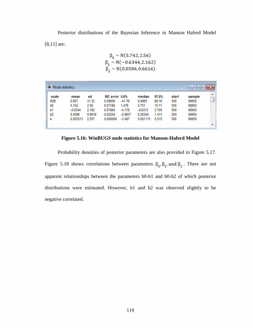
119
Posterior distributions of the Bayesian Inference in Manson Haferd Model
[8,11] are:
Figure 5.16: WinBUGS node statistics for Manson-Haferd Model
Probability densities of posterior parameters are also provided in Figure 5.17.
Figure 5.18 shows correlations between parameters There are not
apparent relationships between the parameters b0-b1 and b0-b2 of which posterior
distributions were estimated. However, b1 and b2 was observed slightly to be
negative correlated.
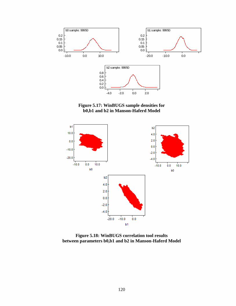
120
b0 sample: 99950
-10.0 0.0 10.0
0.0
0.05
0.1
0.15
0.2
b1 sample: 99950
-20.0 -10.0 0.0
0.0
0.05
0.1
0.15
0.2
b2 sample: 99950
-4.0 -2.0 0.0 2.0
0.0
0.2
0.4
0.6
0.8
Figure 5.17: WinBUGS sample densities for
b0,b1 and b2 in Manson-Haferd Model
Figure 5.18: WinBUGS correlation tool results
between parameters b0,b1 and b2 in Manson-Haferd Model

121
b0
lag
0 20 40
-1.0
-0.5
0.0
0.5
1.0
b1
lag
0 20 40
-1.0
-0.5
0.0
0.5
1.0
b2
lag
0 20 40
-1.0
-0.5
0.0
0.5
1.0
Figure 5.19: WinBUGS autocorrelation results
between parameters b0, b1 and b2 in Manson-Haferd Model
In Figure 5.19, autocorrelation tool results for are provided.
Those results are helpful to understand the performance of the sampler. In this figure,
it is seen that there is a little autocorrelation in the parameters of which posterior
distributions are predicted. However, this followed a decreasing trend in consequent
chains. Running longer chain and thinning have been helpful. Therefore, performance
of the sampler was acceptable. Sampling history of each parameter evaluated in this
model was provided in Appendix D-IV. Those history reports also present a good
sampling performance. Therefore, it was understood that the distributions which were
reached in the end of the sampling were acceptable.
5.2.5 Wilshire Model
Wilshire Model [9-11] is presented in Eq.(5.23). This form of the model was
used in consequent Bayesian Inference framework steps. is the apparent activation
energy calculated for each of the creep-fatigue tests in this study. The average of the
for three consecutive strain controlled creep-fatigue tests was found to be 263,917
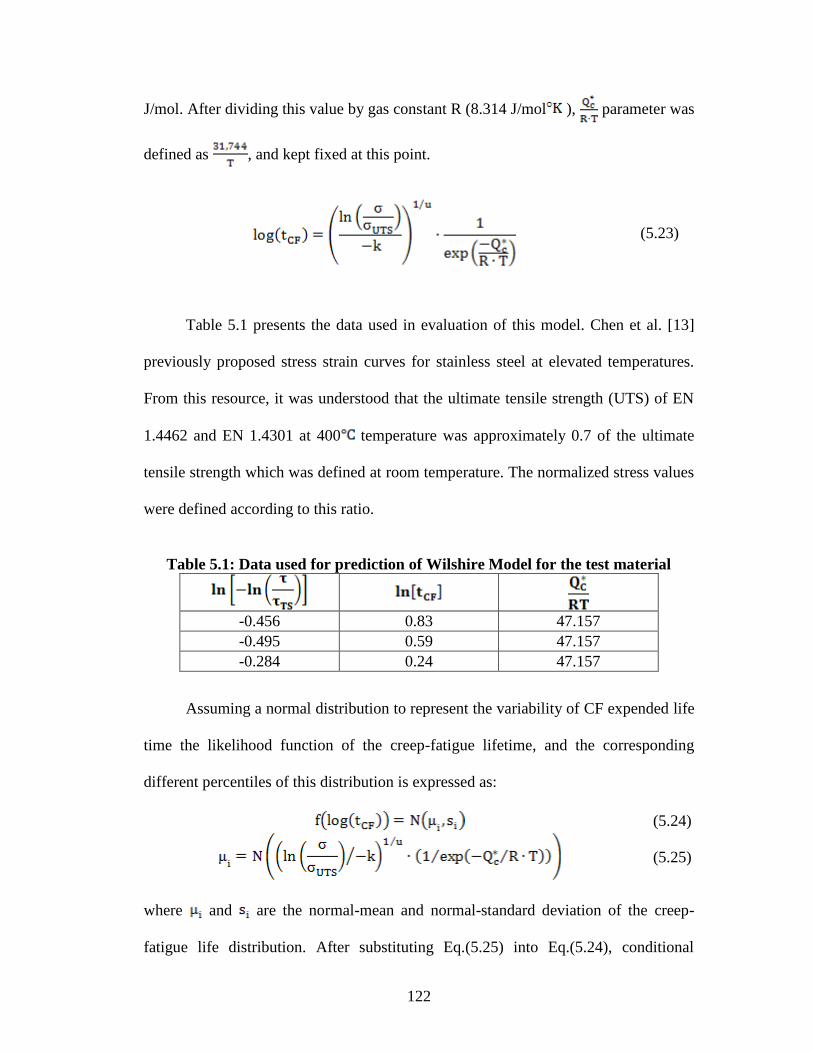
122
J/mol. After dividing this value by gas constant R (8.314 J/mol ), parameter was
defined as , and kept fixed at this point.
(5.23)
Table 5.1 presents the data used in evaluation of this model. Chen et al. [13]
previously proposed stress strain curves for stainless steel at elevated temperatures.
From this resource, it was understood that the ultimate tensile strength (UTS) of EN
1.4462 and EN 1.4301 at 400 temperature was approximately 0.7 of the ultimate
tensile strength which was defined at room temperature. The normalized stress values
were defined according to this ratio.
Table 5.1: Data used for prediction of Wilshire Model for the test material
-0.456 0.83 47.157
-0.495 0.59 47.157
-0.284 0.24 47.157
Assuming a normal distribution to represent the variability of CF expended life
time the likelihood function of the creep-fatigue lifetime, and the corresponding
different percentiles of this distribution is expressed as:
(5.24)
(5.25)
where and are the normal-mean and normal-standard deviation of the creep-
fatigue life distribution. After substituting Eq.(5.25) into Eq.(5.24), conditional

123
distribution function of the creep-fatigue life distribution given normalized stress
condition and test temperature becomes:
(5.26)
Therefore, likelihood function is given by Eq.(5.5). In addition to Eq.(5.5),
posterior distribution of parameters k, u can be derived by using Bayes’ estimation
according to:
(5.27)
where is the subjective prior distribution. Prior distributions are updated
using the experimental data from experiments. Codes written in WinBUGS for
Bayesian Inference of parameters from Wilshire Model [9-11] were provided in
Appendix C-V. In Figure 5.20, WinBUGS node statistics for Wilshire Model [9-11]
are presented.
Figure 5.20: WinBUGS node statistics for Wilshire Model
Posterior distributions of the Bayesian Inference in Wilshire Model [9-11] are:
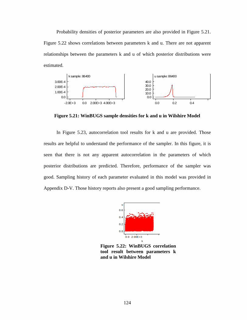
124
Probability densities of posterior parameters are also provided in Figure 5.21.
Figure 5.22 shows correlations between parameters k and u. There are not apparent
relationships between the parameters k and u of which posterior distributions were
estimated.
k sample: 86400
-2.0E+3 0.0 2.00E+3 4.00E+3
0.0
1.00E-4
2.00E-4
3.00E-4
u sample: 86400
0.0 0.2 0.4
0.0
10.0
20.0
30.0
40.0
Figure 5.21: WinBUGS sample densities for k and u in Wilshire Model
In Figure 5.23, autocorrelation tool results for k and u are provided. Those
results are helpful to understand the performance of the sampler. In this figure, it is
seen that there is not any apparent autocorrelation in the parameters of which
posterior distributions are predicted. Therefore, performance of the sampler was
good. Sampling history of each parameter evaluated in this model was provided in
Appendix D-V. Those history reports also present a good sampling performance.
Figure 5.22: WinBUGS correlation
tool result between parameters k
and u in Wilshire Model

125
k
lag
0 20 40
-1.0
-0.5
0.0
0.5
1.0
u
lag
0 20 40
-1.0
-0.5
0.0
0.5
1.0
Figure 5.23: WinBUGS autocorrelation results
for parameters k and u in Wilshire Model.
5.3 References
[1] Modarres, M., Kaminskiy, M, Krivtsov, V., Reliability Engineering and
Risk Analysis, A Practical Guide, CRC Press, 2nd
Edition, 2010.
[2] Ntzoufras, I., Bayesian Modelling Using WinBUGS, In. Giudici, P., Givens,
G.H. and Mallick, B.K. (Eds.), John Wiley & Sons, Inc., Canada, 2009.
[3] Wendell, F., A Handbook on Accelerated Testing, In Fulfillment of the
Scholarly Paper Requirement for the Degree of Master of Science in
Reliability Engineering, Modarres, M. (Adv.), Department of Mechanical
Engineering, University of Maryland, College Park.
[4] Trunin, I.I., Golobova, N.G., Loginov, E.A., “New method of extrapolation
of creep test and long time strength results,” In: Proceedings of the Fourth
International Symposium on Heat-Resistant Metallic Materials, Mala Fatra,
CSSR, p:168,1971.
[5] Larson, F.R., Miller, J., ”A time-temperature relationship for rupture and
creep stress,” Trans. ASME, Vol.74, p:765, 1952.
[6] Eno, D.R., and Young, G.A., “A unified view of engineering creep
parameters,” Proceedings of PVP2008, ASME Pressure Vessels and Piping
Division Conference, July 21-31, Chicago, Illinois, 2008.
[7] Orr, R.L., Sherby, O.D., Dorn, J.E., “Correlation of rupture data for metals
at elevated temperatures,” Trans. ASM, Vol:46, p:113, 1954.
[8] Manson, S.S., Haferd, A.M., “A linear time-temperature relation for
extrapolation of creep and stress rupture data,” NASA TN, 2890, 1953.
[9] Wilshire, B., Scharning, P.J., Hurst, R., “A new approach to creep data
assessment,” Materials Science and Engineering A, Vol:3, Issule:6, pp:510-
511, 2009.

126
[10] Holmstrom, S., “Engineering Tools for Robust Creep Modeling, ” PhD
Dissertation, VTT Publications 728, The Faculty of Engineering and
Architecture, The Aalto University School of Science and Technology,
Espoo, Finland, 2010.
[11] Holdsworth, S.R. and Davies, R.B., “A recent advance in the assessment of
creep rupture data,” Nuclear Engineering and Design, Vol.190, pp:287-296,
1999.
[12] Takashi, Y., Shibamoto, H., Inoue, K., “Long-term creep rupture behavior
of smoothed and notched bar specimens of low-carbon nitrogen-controlled
316 stainless steel (316 FR) and their evaluation,” Nuclear Engineering and
Design, Vol.238, pp:310-321, 2008.
[13] Chen, J. and Young, B., “Stress-strain curves for stainless steel at elevated
temperatures,” Engineering Structures, Vol.28, pp: 229-239, 2006.

127
Chapter 6: Assessment of Creep-Fatigue and Creep in
Cyclic Relaxation
6.1 Introduction
The robust creep-fatigue (CF) model idea initiated by Holmstrom [6] is further
evaluated in this chapter under the section separated for creep-fatigue life curves.
Creep rupture models previously applied in common creep deformation problems
presented good performance with CF life data for the steel alloy. The model [6]
derived from Wilshire model was approved to work with minimum data in this study.
Nevertheless, it was observed that Bayesian inference also could propose feasible
predictions despite of the insufficient data problem as long as proper prior
distributions were initially determined for the predicted model parameters. Therefore,
creep rupture models evaluated on CF data presented high goodness of fit values in
this study. Section 6.2 presents the details of this prediction feasibility investigation.
Section 6.3 confirms that the activation energies obtained for the three CF test
with different hold times for 10, 14 and 21 min are compatible with the published
values given for steel materials.
Section 6.4 is divided into four sub-sections. In Section 6.4.1, creep in cyclic
relaxation response under CF conditions is evaluated. The main difference with
respect to well-known monotonic creep is that the total strain is constant in tensile
hold test on the stress changes with time, whereas the stress is constant in monotonic
creep. It may be possible to interpret the stress dependence of the rate change
throughout the hold time. It was previously shown that the creep mechanism was
identical with that of steady-state in monotonic creep after a substantial hold time.

128
However, in this steady-state monotonic creep time dependency is neglected
regarding the three consecutive regions on a regular creep deformation. Therefore, the
applicability of the some highly feasible time dependent creep models (Norton Bailey
[10], Nuhi’s Empirical [8] and Modified Theta [12]) were investigated on the creep
curves derived from the cyclic relaxation response under CF condition. In Section
6.4.2, probability of exceedance estimation at strain 0.006 [mm/mm] is provided. In
the following Section 6.4.3, the simple definition of CF damage proposed by
Holmstrom [6] for model was applied on the Soviet model. Finally, a remaining
useful life estimation based on the deterministic framework is presented with respect
to a service aged secondary superheater in service conditions.
6.2 CF Expended Life Curves
The probabilistic parameters proposed in Chapter 5 were used in this section to
project CF at the specified test temperature 673.25 (400 ). The master curves are
presented in the order according to the R2B results presented in Chapter 5: Soviet,
Larson-Miller, Orr-Sherby Dorn, Manson Haferd and Wilshire Model. The goodness
of fit for the each of those life prediction models was evaluated in the end of this
section. The results obtained were confirming the R2B results proposed in Chapter 5.
Therefore, the creep life models performed well adaption on the life assessment of CF
life for the steel alloy used in this study.
6.2.1 Soviet Model
Soviet Model [1] was evaluated in Chapter 5 in terms of the derivation of
probabilistic model parameters. Model form is presented in Eq.(6.1). It was observed

129
that and had the least effect in curvature of the model. Therefore, those
parameters were kept as fixed constants. Table 6.1 presents mean and coefficient of
variation results of normally distributed model parameters. Figure 6.1 and Figure 6.2
show the CF life curve and 3D life graph of the model prediction at
673.15 .
(6.1)
Table 6.1: Soviet Model Bayesian parameters and their coefficient of variation
Bayesian
Parameter -8.922 3.795 -3.627
Coefficient
of variation 0.349 0.134 0.655
Figure 6.1: Soviet Model creep – fatigue expended life
curve for steel alloy at 673.15

130
Figure 6.2: Soviet Model creep – fatigue 3D life graph for the steel
alloy at 673.15
6.2.2 Larson-Miller Model
Larson-Miller Model [2] was evaluated in Chapter 5 in terms of the derivation
of probabilistic model parameters. Model form is presented in Eq.(6.2). parameter
in this model is equal to –C. C is the constant in Larson-Miller parameter equation
(see, Eq.(6.3)) [2]. In this study C constant was fixed at 20. Table 6.2 presents mean
and coefficient of variation results of normally distributed model parameters. Figure
6.3 and Figure 6.4 show the CF life curve and 3D life graph of the model prediction
at 673.15 .
n=2, k=0,1,2 (6.2)
(6.3)
Table 6.2: Larson-Miller Model Bayesian parameters and their coefficient of
variation
Bayesian
Parameter 0.0361 13600 -3283
Coefficient of
variation 88.172 2.298E-4 9.16E-4

131
Figure 6.3: Larson-Miller Model creep – fatigue
expended life curve for the steel alloy at
673.15
Figure 6.4: Larson-Miller Model creep – fatigue 3D life
graph for the steel alloy at 673.15
6.2.3 Orr-Sherby Dorn
Orr-Sherby Dorn Model [3] was evaluated in Chapter 5 in terms of the
derivation of probabilistic model parameters. Model form is presented in Eq.(6.4).
parameter in this model is equal to . is the apparent activation energy calculated
for each of the CF tests in this study. The average of the for three consecutive

132
strain controlled CF tests was 263,917 J/mol in this study. After dividing this value by
gas constant R (8.314 J/mol ), parameter was defined as 31,744 and kept fixed at
this point. Table 6.3 presents mean and coefficient of variation results of normally
distributed model parameters. Figure 6.5 and Figure 6.6 show the CF life curve and
3D life graph of the model prediction at 673.15 .
(6.4)
Table 6.3: Orr-Sherby Dorn Bayesian parameters and their coefficient of
variation
Bayesian
Parameter -39.43 -3.04 0.01258
Coefficient of
variation 0.0702 0.8125 76.717
Figure 6.5: Orr-Sherby Dorn Model creep – fatigue
expended life curve for the steel alloy at
673.15

133
Figure 6.6: Orr-Sherby Dorn Model creep – fatigue 3D
expended life graph for the steel alloy at 673.15
6.2.4 Manson Haferd Model
Manson Haferd Model [4] was evaluated in Chapter 5 in terms of the
derivation of probabilistic model parameters. Model form is presented in Eq.(6.5).
parameter of this model was kept fixed at 666.5. Additionally, was kept fixed at -
29.9. Since the limited data were available in this study fixing the least contributing
parameters helped further investigation of this model. Table 6.4 presents mean and
coefficient of variation results of normally distributed model parameters. Figure 6.7
and Figure 6.8 show the CF life curve and 3D life graph of the model prediction at
673.15 .
n=2, k=0,1,2 (6.5)
Table 6.4: Manson Haferd Model Bayesian parameters and their coefficient of
variation
Bayesian
Parameter 5.742 -0.6344 0.0585
Coefficient of
variation 0.4458 3.4079 11.309

134
Figure 6.7: Manson Haferd Model creep – fatigue
expended life curve for the steel alloy at
673.15
Figure 6.8: Manson Haferd Model creep – fatigue 3D
expended life graph for the steel alloy at
673.15
6.2.5 Wilshire Model ( Model)
Wishire Model [5] was evaluated in Chapter 5 in terms of the derivation of
probabilistic model parameters. Model form is presented in Eq.(5.26). is the
apparent activation energy calculated for each of the CF tests in this study. The
average of the for three consecutive strain controlled CF tests was found to be
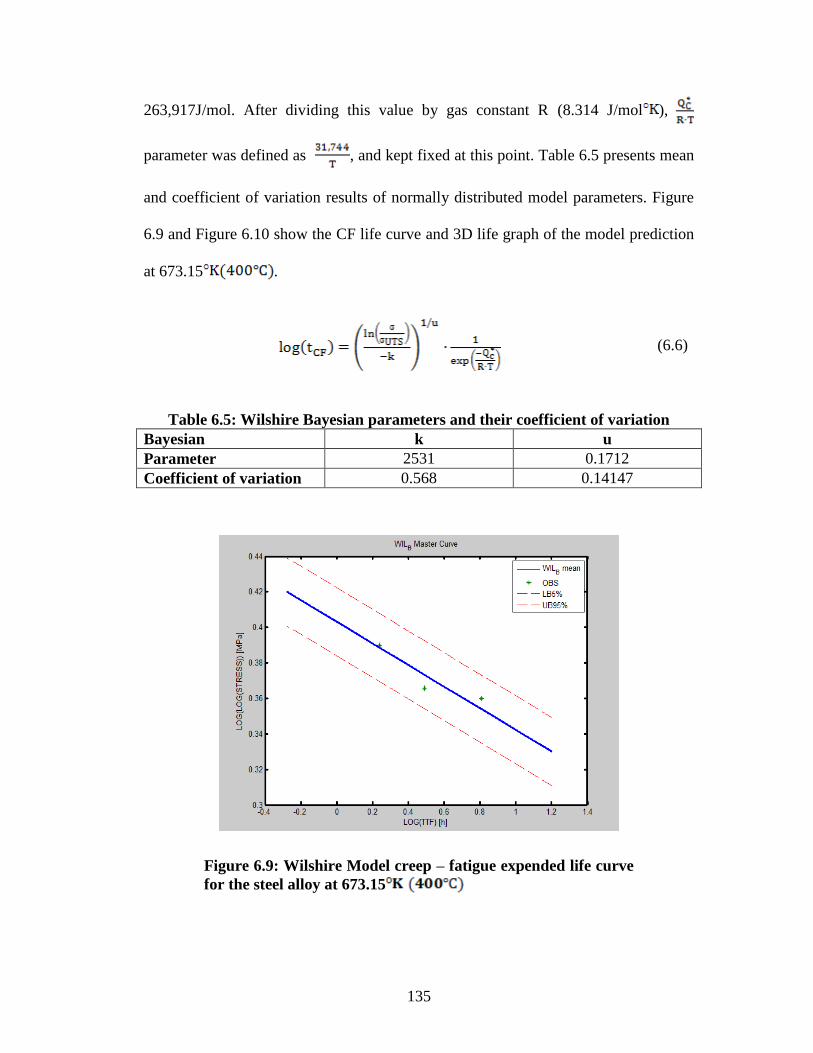
135
263,917J/mol. After dividing this value by gas constant R (8.314 J/mol ),
parameter was defined as , and kept fixed at this point. Table 6.5 presents mean
and coefficient of variation results of normally distributed model parameters. Figure
6.9 and Figure 6.10 show the CF life curve and 3D life graph of the model prediction
at 673.15 .
(6.6)
Table 6.5: Wilshire Bayesian parameters and their coefficient of variation
Bayesian k u
Parameter 2531 0.1712
Coefficient of variation 0.568 0.14147
Figure 6.9: Wilshire Model creep – fatigue expended life curve
for the steel alloy at 673.15

136
Figure 6.10: Wilshire Model creep – fatigue 3D expended life
graph for the steel alloy at 673.15
6.2.6 Comparison of CF Life Models
Figure 6.11 presents the comparison of CF life (creep rupture) models for the
steel alloy. In Figure 6.11, the stress for the assessed material is shown as a function
of temperature-compensated life ( for creep or for CF). Homström et al. [6]
notes also that predicted time to creep rupture and time to CF failure fall on
the same material-specific curves.
Figure 6.11: Time to CF failure comparison for the steel alloy

137
The goodness of fit can be expressed as the scatter factor Z [6-7]. The scatter
factor Z formula is given in Eq.(6.7):
(6.7)
where n is the number of data points. In this study, the agreement between predicted
and observed CF life is very good as for all of the model predictions Z 4.93.
Assuming normal distribution for CF life, the observed log(NCF) would lie in almost
99% of the observed times within predicted log(NCF) log(Z). A comparison of the
predicted vs. observed CF life in terms of cycles to failure is shown in Figure 6.12.
Figure 6.12: Predicted vs. observed CF expended life for the steel alloy

138
6.3 Assessment of Creep Activation Energy of Test Material
Larson-Miller parameter [2] helps to estimate the creep activation energy of
materials. It can be derived from Dorn relation [3].
(6.8)
where A, n are constants, R is the gas constant, T is the absolute temperature in
Kelvin, is the external applied stress, is the activation enthalpy of creep process,
and is the secondary strain rate. Faridani [8] explains the formula derivation for
creep activation energy with respect to the Larson Miller parameter relation as
follows.
(6.9)
Taking logarithms from both sides, results in:
(6.10)
or
(6.11)
Then by a given stress (constant value):
(6.12)
The Larson-Miller parameter is give by:
(6.13)
Activation energy (Q) of the test material is calculated by taking C=20 for
static creep and values observed in consecutive CF tests at

139
. Table 6.6 presents the activation energies which were
calculated for each CF tests with 10, 14 and 21 min hold time at the fixed test
temperature 673.15 .
Table 6.6: Activation energies for different hold-times at 673.15
Test No Temperature ( ) Hold Time (min) Q (J/mole)
1 673.15 10 267,883
2 673.15 14 263,322
3 673.15 21 260,546
Q values presented above are in good agreement with the published values
given for steel materials (245-399 kJ/mol) [9].
6.4 Assessment of Creep under CF Condition
This section is divided into four sub-sections. In the first sub-section, creep in
cyclic relaxation response under CF conditions is evaluated. The main difference is
that the total strain is constant in tensile hold test on the stress is changed with time,
whereas the stress is constant in monotonic creep. It may be possible to interpret the
stress dependence of the rate change throughout the hold time. It was previously
shown that the creep mechanism was identical with that of steady-state in monotonic
creep after enough hold time. However, in this steady-state monotonic creep time
dependency is neglected regarding the three consecutive regions on a regular creep
deformation. Therefore, the applicability of the some highly feasible time dependent
creep models (Norton Bailey [1929-1935, 2003], Nuhi’s Empirical [8] and Modified
Theta [12]) was investigated on the creep curves derived from the cyclic relaxation
response under CF condition. In the second sub-section, probability of exceedance
estimation at strain 0.006 [mm/mm] is provided. In the following third sub-section,
140
the simple definition of CF damage proposed by Holmstrom [6] for model was
applied on Soviet model. Finally, a remaining useful life estimation based on the
deterministic framework is presented with respect to a service aged secondary
superheater in service conditions.
6.4.1 Creep in Cyclic Relaxation Response under Creep Fatigue Conditions
In this section, the creep behaviors of stress relaxation in steel alloy during
hold time cycled at high temperature (673.15 ) have been analyzed. Finally, the
prediction performance of the well-known constitutive equations for creep
deformation of stress relaxation in the test metal was compared, and degradation
versus time graph was drawn to see the trend of creep deformation in cyclic
relaxation response.
It has been a benefit that a large amount of creep information can be obtained
from the short term of a relaxation test [9]. Since relaxation during most of the tests
occurred in cyclically hardened materials, it would have been more appropriate to
relate creep damage to stress-rupture curves for material that had been cyclically
hardened [9]. For many types of cyclic operation at elevated temperature, the loading
history can be approximated by a strain cycle followed by a hold period at constant
strain with stress relaxation as illustrated in Figure 3.8 [9]. Determination the form of
the relaxation curve is explained in Chapter 3.
Analyzing the value of the activation volume for the initial transient relaxation
behavior in which the stress is relaxed drastically, it has been suggested that the rate
controlling the dislocation mechanism is either cross slip, or overcoming Peierls-
Nabarro stress. Thus the temperature dependence of creep rate was identified during

141
stress relaxation. It was shown that the creep mechanism is identical with that of
steady state in monotonic creep after a long enough hold time, which is the
dislocation climb controlled by self diffusion [11]. So if dislocation creep is
considered, the strong dependence of creep rate on the applied stress is observed. The
main difference is that the total strain is constant in tensile hold test and the stress is
changed with time, whereas the stress is constant in monotonic creep. Therefore, it
may be possible to interpret the stress dependence of the rate change throughout the
hold time [11].
Figure 6.13: results for Norton Bailey, Nuhi’s Empirical and
Modified Theta Models
Figure 6.13 shows results for Norton Bailey [1929-1935, 2003], Nuhi’s
Empirical [8] and Modified Theta Models [12] respectively in each CF test with 10,
14 and 21 min hold times. Since only isothermal relaxation and creep response are
treated in this section, the two of the equations evaluated do not include the
temperature variable T. In general applications, temperature should be included.

142
Since the goal of this section is to initially investigate the feasibility of predicting
creep curves from relaxation test results, the closed form of well known creep
expressions for the relaxation curve were evaluated. According to the results in
Figure 6.13, Nuhi’s Empirical Model which was proposed in Ref.[8] presented the
best fit throughout the all CF tests. Figure 6.14 shows the creep curves in cyclic
relaxation response under CF conditions for 10min (CF Test#1), 14min (CF Test#2)
and 21min (CF Test#3) hold times at 673.155 according to the Nuhi’s
Empirical model. The threshold level of 0.006 was defined according to the average
useful life results for the three CF tests conducted. It was predicted that nearly after
this level the tertiary part of creep curve began.
Figure 6.14: Creep curves in cyclic relaxation response under CF conditions
for 10min (CF Test#1), 14min (CF Test#2) and 21min (CF Test#3) hold times
at 673.155
6.4.2 Probability of Exceedance Estimation at Strain 0.006 [mm/mm]
Severe structural deformation of material begins at the end point of the
secondary region or the beginning point of the tertiary region. At this level, most of

143
the cavities begin to agglomerate and forms a crack. In this section, exceedance
probability of 0.006 [mm/mm] strain level was calculated for different hold times. A
MATLAB code was written to calculate the probability of exceedance at iterative
time points for the strain levels beyond the threshold strain of 0.006 [mm/mm] for the
steel alloy (see, Figure 6.16).
Table 6.7 presents the probability of exceedance for 0.006 [mm/mm] at
different times observed in CF test # 3. From this table it is understood that the test
specimen was exposed to a considerable amount of creep damage at 13278.22s (3.415
h).
Figure 6.15: Normal cdf at strain 0.006 [mm/mm] for creep
in cyclic relaxation response under CF conditions for 10min
(CF Test#1), 14min (CF Test#2) and 21min (CF Test#3) hold
times at 673.155

144
Table 6.7: Probability of exceedance at strain 0.006
[mm/mm] for different times at CF test # 3 (21min hold
time)
CF TEST#3
Time [s]
13565 0.54
13278 0.49
12995 0.45
12712 0.41
10907 0.21
6.4.3 Damage Assessment in CF
Holmstrom [6] proposes a simple definition of CF damage. In this definition
there is no need to separate creep or fatigue damage or life fractions. This simple
definition also allows for more straightforward damage assessment for both design
and later life assessment than the common methods using summed life (or strain)
fractions. This simple definition for simultaneous CF damage is given in Eq.(6.13).
Table 6.8: Cumulative creep damage in each CF cycle for 21min hold time CF
Test#3
CF Test # 3 Cycles
1 2 3 4 5
0.22 0.44 0.65 0.87 1.09
Table 6.8 presents the cumulative creep damage in each simultaneous CF cycle
for the last 21min hold test according to this equation. values was calculated for
the maximum stresses observed in each expended cycle of CF test. As the life
equation, Soviet Model was chosen since it gave the highest fit for the observed CF
145
data. All the cumulative hold times were normalized according to the Soviet Model
result for the maximum stress level observed during the test.
(6.14)
6.4.4 Remaining Useful Life in Deterministic Framework
Banerjee et al. [13] previously investigated applicability of a physics based
prognostics approach for solder joints using microstructural damage models. In their
work, a PCB consisting of a heat generating chip with Ball-Grid Array (BGA) solder
joints was considered for avionics application. They calculated remaining useful life
(RUL) from the damage for creep and fatigue loads (D) and total mission duration
time (tM) as given in Eq.(6.17).
(6.15)
The test data in this study was evaluated with respect to the service-aged
superheater used in Ref. [14] to apply the deterministic remaining useful life formula
that was derived in Ref. [13]. The service-aged superheater header has the service
properties listed in Table 6.9.
Figure 6.16 shows the acceleration factor trend with respect to the use level
stress 17.3 MPa. The acceleration factor versus stress plot displays the acceleration
factor as a function of stress based on the specified use stress level. The acceleration
factor is a ratio of the use stress level divided by the accelerated stress levels which
were the maximum stress levels observed during the each CF tests.

146
Table 6.9: Basic details of the service-aged secondary
superheater [14]
Material 2.25Cr-1Mo (JIS STPA24)
Operation temperature 569
Operation pressure 17.3MPa
Operated hour 163,000hr
Dimension 508mm in OD x 272mm in ID
After the extrapolating damage trend, which was observed in the creep fatigue
tests conducted, to the proposed service stress level 17.3MPa, the damage was
predicted as 0.63 regarding the service conditions defined in Ref. [14]. The RUL was
predicted as 95,730 h. Therefore, the inspection time should be chosen nearly at this
operation time which was predicted by the Eq.(6.15).
Accurate prediction of RUL would enable a user to gauge the health of an
existing unit and optimally plan maintenance schedules as well as help in designing
the unit to withstand the loads for the intended application.
Figure 6.16: Acceleration factor graph with respect to
the specified use level stress 17.3 MPa

147
6.5 References
[1] Trunin, I.I., Golubova, N.G. & Loginov, E.A., “A new method of the
extrapolation of creep-test and long-time strength results,” Proc 4th
Int Symp
on Heat-Resistant Metallic Materials, Mala Fatra, CSSR, pp. 168-176, 1971.
[2] Larson, F.R., Miller, E.J., “Time-temperature relationship for rupture and
creep stresses,” Trans. ASME, vol.74, p.765-775, 1952.
[3] Orr, R.L., Sherby, O.D., Dorn, J.E., “Correlations of rupture data for metals at
elevated temperatures,” Trans. ASM, vol.46, pp:113-118, 1954.
[4] Manson,S.S., Haferd, A.M., “A linear time-temperature relation for
extrapolation of creep and stress rupture data,” NACA TN 2890, 1953.
[5] Wilshire, B., Scharning, P.J., Hurst, R., “A new approach to creep data
assessment,” Materials Science and Engineering A, Vol.510-511, Issue:3-6,
2009.
[6] Holmström, S., Auerkari, P., “A robust model for creep-fatigue life
assessment,” Materials Science & Engineering A, Vol.559, pp:333-335, 2013.
[7] Holdsworth, S.R. (Ed.), ECCC Recommendations, Vol.5, 2005.
[8] Faridani, M.N. and Modarres, M., “Classification and probabilistic model
development for creep failures of structures: study of X-70 carbon steel and
7075-T6 aluminum alloys,” Thesis, In partial fulfillment of the
requirements of the degree of Master of Science, Fall 2011.
[9] Syn, C.K., Lesueur, D.R., Sherby, O.D., Taleff, E.M., “Stress-strain rate
relations in ultrahigh carbon steels deformed in the ferrite range of
temperature,” Materials Science Forum, Vol.426-432, pp:853-858, 2003.
[10] Jaske, C.E., Mindlin, H., and Perrin, J.S., “Combined Low-Cycle Fatigue and
Stress Relaxation of Alloy 800 and Type 304 Stainless Steel at Elevated
Temperatures,”Fatigue at Elevated Temperature, ASTM STP 520, American
Society for Testing Materials, pp:365-376, 1973.
[11] Jeong, C.Y., Nam, S.W., “Stress dependence on stress relaxation creep rate
during tensile holding under creep-fatigue interaction in 1Cr-Mo-V steel,”
Journal of Material Science, Vol.34, pp:2513-2517, 1999.
[12] Evans, R.W., and Wilshire, B., “Creep of metals and alloys,” Institute of
Metals, 1985.

148
[13] Banerjee, A., Koul, A., Kumar, A. and Goel, N., “Physics based Prognostics
of Solder Joints in Avionics,” Annual Conference of the Prognostics and
Health Management Society, 2011.
[14] Takagi, Y., Otsuki, S., “Creep-fatigue characteristics of partial repair welds
and full repair welds on aged 2.25Cr-1Mo Steel,” CMMI, Vol.3, Issue:1,
2004.

149
Chapter 7: Conclusions and Recommendations
for Future Work
Creep-fatigue (CF) expended life models were derived and validated using
experimental results for an steel alloy. The robust CF expended life model was first
used along with the CF of ferritic steel P91, austenitic steel, and Ni alloy by [1]. The
predictions compared well with the experimental results within a scatter band close to
factor of 2. This demonstrates the predictive capability of CF expended life models
modified in this thesis. Uncertainties of each parameter predicted were defined using
the Bayesian inference framework. Validation of simultaneous CF loading expended
life models - apart from modified Wilshire model proposed by Holmstrom [1] - was
accomplished in this study. The most of the previous studies have been focused
mainly on the sequential CF loading expended life models. These modified models
are based on the creep rupture behavior, and their input parameters are described by
the hold time in tension, and maximum stress observed in each CF test. The creep
behavior of cyclic relaxation response in the steel alloy under CF conditions was also
analyzed.
A summary of accomplished tasks are presented below.
1. Existing creep-rupture models other than Wilshire were modified to
simultaneous CF loading expended life models.
2. Isothermal CF tests under strain control, with stress ratio R=0 and hold
periods in tension were conducted on steel alloy samples to validate the CF
expended life models modified.
3. The suggested CF expended lifetime approach by Holmstrom [1] was

150
confirmed in this study as an effective CF expended lifetime.
4. The modified CF expended life models were shown to predict the observed
CF expended life of the tested material steel alloy sample with a scatter band
close to a factor of 2.
5. CF expended life of the steel alloy was found to decrease with increase in hold
time under strain control.
6. Modified CF expended life models were evaluated under Bayesian inference
framework using experimental data, and posterior distributions of the
predicted parameters were proposed assuming a normally distributed
likelihood function.
7. Uncertainties of the predicted CF expended life model parameters were
defined using Bayesian inference results.
8. Activation energies (Q values) in different hold times at 673.15 K (400 C )
were calculated. It was observed that Q values were in good agreement with
the published values for steel materials (245-399 kJ/mol).
9. The creep behavior of cyclic relaxation response in the steel alloy under CF
conditions was analyzed for the overall CF expended life for each experiment.
The prediction performance of the well known constitutive equations was
compared based on the experimental results. Details can be further reviewed
in Section 6.4. It was observed that the main difference between creep in
cyclic relaxation response and monotonic creep stems from total strain and
stress change with respect to time. Creep in cyclic relaxation response
demonstrates a constant total strain and changing stress until the specified end

151
criterion for the CF test. However, monotonic creep demonstrates a constant
stress and changing total strain until rupture.
10. At strain 0.6%, probability of exceedance for different times in CF test with
21 min hold time was estimated. It was understood that the test sample was
exposed to a considerable amount of creep damage at 13278.22s (3.415h) at
CF test with 21 min hold time.
11. Damage assessment in simultaneous CF loading was estimated according to
the approach proposed by Holmstrom [1]. This approach does not need
separation in CF damage or expended life. In order to predict the expected CF
expended life for each peak stress observed in CF cycles, the results provided
in Section 5.2 were referred to. Among the modified CF expended life models
which performed acceptable prediction performance on the test material, the
Soviet Model was chosen to evaluate damage assessment for CF test with 21
min hold time.
12. A remaining useful life example in deterministic framework was presented.
Accurate prediction of Remaining Useful Life (RUL) would enable a user to
gauge the health of an existing unit and optimally plan maintenance schedules
as well as help in designing the unit to withstand the loads for the intended
application.
Recommendations for future work:
1. Additional CF tests at room temperature could help observe how stable the
stress relaxation response in each CF experiments performed in this study
was. This could also help understand the noise pattern in CF data at elevated
152
temperature, and could also provide more accurate characterization of creep
behavior.
2. In the course of model validation, it was understood that additional hot tension
tests at the specified test temperature would help understand the exact high-
temperature mechanical properties of the concerned test material. In that case,
the Wilshire model could yield a higher goodness of fit since it was observed
that Wilshire model provided the highest coefficient of determination value
based on the CF data provided in Ref.[2]. There might also be material
dependence affecting the prediction of Wilshire model. Additional hot tension
tests at pre-determined test temperatures prior to starting the actual CF
experiments would help device a better test plan, and also help understand the
prediction performance of the proposed models with respect to the changing
material properties.
3. The validity of data can be examined with respect to reproducibility between
tests. More test samples are needed to perform this. It may be worthy to
investigate the reproducibility of these CF tests to understand validity of the
test data from this perspective.
4. CF tests can be initially modeled using finite element software packages such
as ANSYS or Abaqus. The results from these simulations can be compared to
actual experimental results.
7.1 References
[1] Holmström, S., Auerkari, P., “A robust model for creep-fatigue life
assessment,” Materials Science & Engineering A, Vol.559, pp:333-335, 2013.

153
[2] Takashi, Y., Shibamo, H., and Inoue, K., “Long-term creep rupture vebahiour
of smoothed and nothched bar specimens of low-carbon nitrogren-controlled
316 stainless steel (316FR) and their evaluation,” Nuclear Engineering
Design, Vol.238, 00:310-321, 2008.

154
Appendix A-I: Thermocouple Clip Design Process
The simplest way to measure the temperature in a 600 C furnace is to use a
thermocouple. For this experimental work, the temperature at the surface of the metal
test pieces, in particular in the reduced diameter section is of particular interest. Two
temperature measurements were made one at the top of the sample (far away from the
reduced diameter section) and another at the surface of the reduced diameter section.
There are two standard ways to attach the thermocouples to the samples glue and a
metal clip, analogous to the original wooden clothes peg, the latter was chosen for
this work. Small stainless steel clips (single piece, no moving parts) which had a dual
feature to ensure the spherical thermocouple junction was held against the cylindrical
metal sample were used. One side of peg's gap had a groove to align against the side
of the cylinder, and the other side had a pocket to hold the ball on the tip of the
thermocouple, so pushing the clip on automatically put the thermocouple in the right
place. The thermal mass of the clip was low enough to not affect the heating of the
test piece. Attached thermocouple clip and its design picture are provided in Figure
A-I.1.
(a) (b)
Figure A-I.1: (a) Thermocouple clip attached to test sample, and (b)
thermocouple clip design dimensions

155
Appendix B-I: Epoxy Mold Design Process
Due to lack of existing epoxy molds to fit into the polishing machine, custom
epoxy molds were created using polyethylene. . The shape of the epoxy mold was
cylindrical, with diameter 1.25" and height ~0.5". The tolerance of the diameter was
wide (+/-0.010") and the height was nominal (+/- 0.20"). In order to fabricate the
mold, first a 1.5" diameter polyethylene bar was bored out to depth 0.5" and diameter
1.25" leaving a thin walled bottom only 0.020" thick. Next the interior of the mold
was wiped with a thin film of oil to act as a mold release. Then the sample
was placed on the thin-walled bottom and epoxy potting mix (Allied Epoxy Mount
Resin and Hardener) was poured on top to fill up the cup. After curing, the bottom
was pushed, and since it was flexible (due to the thin wall), the cylindrical plug
readily came out making it ready for the polishing machine. The standalone
fabricated epoxy mold and a mounted sample epoxy are shown in Figure B-I.1.
(a) (b)
Figure B-I.1: (a) Epoxy mold produced, (b) mounted sample
using epoxy mold

156
Appendix C-I: WINBUGS Codes for Soviet Model
model{
#Here the prior distributions for the model parameters b0, b1 and b4 as well as
#the prior distribution for s, the standard deviation of normal likelihood, are
#defined. Here, both normal and non-informative uniform distributions are
#preferred.
b0 ~ dnorm(-8.888,0.1)
b1 ~ dnorm(3.789,0.1)
b4 ~ dnorm(-3.612,0.1)
s ~ dunif(0,10)
#Constants are specified.
C<- 1000
b2 <- -8.755E-11
b3 <- -9452
#For likelihood function, a normal distribution is assumed, and it is written
#out, rather than using normal distribution function (dnorm) already part of
# the BUGS code.
for(i in 1 : N) {
zeros[i] <- 0
L[i] <- exp(-0.5 * pow((x[i,2] -
(b0+(b1*log(x0[i]))+(b2*log(x[i,1]))+(b3/x0[i])+(b4*(x[i,1]/x0[i]))))/s,2))/(pow((2 *
3.141592654), 0.5) *s)
ghr[i]<- (-1) * log(L[i]) + C
zeros[i] ~ dpois(ghr[i])
}
#Here it is asked WinBUGS to use the standard deviation from the normal
#likelihood to estimate the 'error' in the model which the data are fitted. For
#the error, e, the normal distribution that is already provided in WinBUGS is
#used. It is assumed that the error has a mean of 0.
tau<-1/pow(s,2)
e~dnorm(0,tau)
#Here the sample variance is calculated.
for(i in 1:N) { c.x1[i] <- x1[i] - mean(x1[])}
sy2 <- inprod(c.x1[], c.x1[])/(N-1)
#Here Bayesian version R squared is calculated.
R2B <- 1 - e/sy2}

157
Appendix C-II: WINBUGS Codes for Larson Miller Model model{
#Here the prior distributions for the model parameters b0, b1 and b2 as well as
#the prior distribution for s, the standard deviation of normal likelihood, are
#defined. Here, both normal and non-informative uniform distributions are
#preferred.
b0 ~ dnorm(-0.00421,0.1)
b1 ~ dnorm(1.36E+4,0.1)
b2 ~ dnorm(-3283,0.1)
s ~ dunif(0,10)
#Constant is specified.
C<- 1000
#For likelihood function, a normal distribution is assumed, and it is written
#out, rather than using normal distribution function (dnorm) already part of
#the BUGS code.
for(i in 1 : N) {
zeros[i] <- 0
L[i] <- exp(-0.5 * pow((x[i,2] - (-
20+(1/x0[i])*(b0+b1*x[i,1]+b2*(pow(x[i,1],2)))))/s , 2))/(pow((2 * 3.141592654) ,
0.5) *s)
ghr[i]<- (-1) * log(L[i]) + C
zeros[i] ~ dpois(ghr[i])
}
#Here it is asked WinBUGS to use the standard deviation from the normal
#likelihood to estimate the 'error' in the model which the data are fitted. For
#the error, e, the normal distribution that is already provided in WinBUGS is
#used. It is assumed that the error has a mean of 0.
tau<-1/pow(s,2)
e~dnorm(0,tau)
#Here the sample variance is calculated.
for(i in 1:N) {c.x1[i] <- x1[i] - mean(x1[])}
sy2 <- inprod(c.x1[], c.x1[])/(N-1)
#Here Bayesian version R squared is calculated.
R2B <- 1 - e/sy2
}
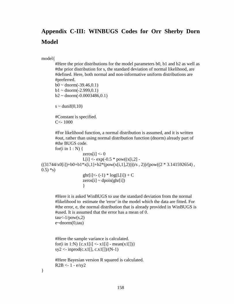
158
Appendix C-III: WINBUGS Codes for Orr Sherby Dorn
Model
model{
#Here the prior distributions for the model parameters b0, b1 and b2 as well as
#the prior distribution for s, the standard deviation of normal likelihood, are
#defined. Here, both normal and non-informative uniform distributions are
#preferred.
b0 ~ dnorm(-39.46,0.1)
b1 ~ dnorm(-2.999,0.1)
b2 ~ dnorm(-0.0003486,0.1)
s ~ dunif(0,10)
#Constant is specified.
C<- 1000
#For likelihood function, a normal distribution is assumed, and it is written
#out, rather than using normal distribution function (dnorm) already part of
#the BUGS code.
for(i in 1 : N) {
zeros[i] <- 0
L[i] <- exp(-0.5 * pow((x[i,2] -
((31744/x0[i])+b0+b1*x[i,1]+b2*(pow(x[i,1],2))))/s , 2))/(pow((2 * 3.141592654) ,
0.5) *s)
ghr[i]<- (-1) * log(L[i]) + C
zeros[i] ~ dpois(ghr[i])
}
#Here it is asked WinBUGS to use the standard deviation from the normal
#likelihood to estimate the 'error' in the model which the data are fitted. For
#the error, e, the normal distribution that is already provided in WinBUGS is
#used. It is assumed that the error has a mean of 0.
tau<-1/pow(s,2)
e~dnorm(0,tau)
#Here the sample variance is calculated.
for(i in 1:N) {c.x1[i] <- x1[i] - mean(x1[])}
sy2 <- inprod(c.x1[], c.x1[])/(N-1)
#Here Bayesian version R squared is calculated.
R2B <- 1 - e/sy2
}

159
Appendix C-IV: WINBUGS Codes for Manson Haferd
Model
model{
#Here the prior distributions for the model parameters b0,b1 and b2 as well as
#the prior distribution for s, the standard deviation of normal likelihood, are
#defined. Here, both normal and non-informative uniform distributions are
#preferred.
b0 ~ dnorm(5.634,0.1)
b1 ~ dnorm(-0.4502,0.1)
b2 ~ dnorm(-1.027E-6,0.1)
s ~ dunif(0,10)
#Constant is specified.
C<- 1000
b5 <- -29.9
Ta <- 666.5
#For likelihood function, a normal distribution is assumed, and it is written
#out, rather than using normal distribution function (dnorm) already part of
#the BUGS code.
for(i in 1 : N) {
zeros[i] <- 0
L[i] <- exp(-0.5 * pow((x[i,2] - (b5+((x0[i]-Ta)*b0)+((x0[i]-
Ta)*(b1*x[i,1]))+((x0[i]-Ta)*(b2*pow(x[i,1],2)))))/s , 2))/(pow((2 * 3.141592654) ,
0.5) *s)
ghr[i]<- (-1) * log(L[i]) + C
zeros[i] ~ dpois(ghr[i])
}
#Here it is asked WinBUGS to use the standard deviation from the normal
#likeihood to estimate the 'error' in the model which the data are fitted. For
#the error, e, the normal distribution that is already provided in WinBUGS are
#used. It is assumed that the error has a mean of 0.
tau<-1/pow(s,2)
e~dnorm(0,tau)
#Here the sample variance is calculated.
for(i in 1:N) { c.x1[i] <- x1[i] - mean(x1[])}
sy2 <- inprod(c.x1[], c.x1[])/(N-1)
#Here Bayesian version R squared is calculated.
R2B <- 1 - e/sy2
}

160
Appendix C-V: WINBUGS Codes for Wilshire Model
model{
#Here the prior distributions for the model parameters k and u as well as the
#prior distribution for s, the standard deviation of normal likelihood, are
#defined. Here, non-informative uniform distributions are preferred.
k~ dunif(0,10000)
u ~ dunif(0,1)
s ~ dunif(0,10)
#Constant is specified.
C<- 1000
#For likelihood function, a normal distribution is assumed, and it is written
#out, rather than using normal distribution function (dnorm) already part of
#the BUGS code.
for(i in 1 : N) {
zeros[i] <- 0
L[i] <- exp(-0.5 * pow((x[i,2] – (pow((x[i,1]/-
k),1/u)*3.0E+20))/s , 2))/(pow((2 * 3.141592654) , 0.5) *s)
ghr[i]<- (-1) * log(L[i]) + C
zeros[i] ~ dpois(ghr[i])
}
#Here it is asked WinBUGS to use the standard deviation from the normal
#likeihood to estimate the 'error' in the model which the data are fitted. For the
#error, e, the normal distribution that is already provided in WinBUGS are
#used. It is assumed that the error has a mean of 0.
tau<-1/pow(s,2)
e~dnorm(0,tau)
#Here the sample variance is calculated.
for(i in 1:N) { c.x1[i] <- x1[i] - mean(x1[])}
sy2 <- inprod(c.x1[], c.x1[])/(N-1)
#Here Bayesian version R squared is calculated.
R2B <- 1 - e/sy2
}

161
Appendix D-I: WINBUGS Chain History for Soviet Model
Parameters
b0
iteration
500 250000 500000 750000
-30.0
-20.0
-10.0
0.0
10.0
b1
iteration
500 250000 500000 750000
0.0
2.0
4.0
6.0
8.0
b4
iteration
500 250000 500000 750000
-20.0
-10.0
0.0
10.0

162
Appendix D-II: WINBUGS Chain History for Larson Miller
Model Parameters
b0
iteration
500 50000 100000
-20.0
-10.0
0.0
10.0
20.0
b1
iteration
500 50000 100000
13580.0
13590.0
13600.0
13610.0
13620.0
b2
iteration
500 50000 100000
-3300.0
-3290.0
-3280.0
-3270.0

163
Appendix D-III: WINBUGS Chain History for Orr-Sherby
Dorn Model Parameters
b0
iteration
500 200000 400000 600000
-60.0
-50.0
-40.0
-30.0
-20.0
b1
iteration
500 200000 400000 600000
-20.0
-10.0
0.0
10.0
b2
iteration
500 200000 400000 600000
-7.5
-5.0
-2.5
0.0
2.5
5.0

164
Appendix D-IV: WINBUGS Chain History for Manson
Haferd Model Parameters
b0
iteration
500 250000 500000 750000
-10.0
0.0
10.0
20.0
b1
iteration
500 250000 500000 750000
-15.0
-10.0
-5.0
0.0
5.0
10.0
b2
iteration
500 250000 500000 750000
-4.0
-2.0
0.0
2.0
4.0

165
Appendix D-V: WINBUGS Chain History for Wilshire
Model Parameters
k
iteration
500 250000 500000 750000
0.0
2.00E+3
4.00E+3
6.00E+3
u
iteration
500 250000 500000 750000
0.0
0.2
0.4
0.6
166
Bibliography
A.S.T.M., “Symposium on the Effect of Cyclic Heating and Stressing on Metals at
Elevated Temperatures,” (Special Tech. Publ. No.165), Philadelphia, Pa. (Amer. Soc.
Test. Mat.), 1954.
Anon. Code Case N-47, ASME boiler and pressure vessel code, “Criteria for design of
elevated temperature,” Class 1 Components in section III, division 1, American Society
of Mechanical Engineers, 1976.
Asayama, T. and Tachibana, Y., “Collect Available Creep-Fatigue Data and Study
Existing Creep-Fatigue Evaluation Procedures for Grade 91 and Hastelloy XR,”
DOE/ASME Generation IV Materials Project, Japan Atomic Energy Agency,
September 30, 2007.
ASTM Standard E2714-09e1, “Standard test method for creep-fatigue testing,” ASTM
International, West Conshohocken, PA, 2009, DOI: 10.1520/E2714-
09EOI,www.astm.org.
ASTM Standard E407-07, “Standard practice for microetching and alloys,” ASTM
International, West Conshohocken, PA, 2007, DOI: 10.1520/E0407-07, www.astm.org.
ASTM Standard E606/E606M, “Standard Test Method for Strain-Controlled Fatigue
Testing,” ASTM International, West Conshohcken, PA, 2012, DOI: 10.1520/E0606-
04E01, www.astm.org .
ASTM Standard E8/E8M-11, “Standard test methods for tension testing on metallic
materials,” ASTM International, West Conshohocken, PA, 2011,
DOI:10.1520/E0008_E0008M-11, www.astm.org.
Baker and Cane model: Baker AJ, O‘Donnell MP. R5 high temperature structural
integrity assessment of a cracked dissimilar metal weld vessel test. In: Proceedings of
second international conference on integrity of high temperature welds, London, 10–12
November 2003.
Banerjee, A., Koul, A., Kumar, A. and Goel, N., “Physics based Prognostics of Solder
Joints in Avionics,” Annual Conference of the Prognostics and Health Management
Society, 2011.

167
BJF-model: Jones, D.I.G, French, R.M. and Bagley, R.L.; A Renewal Theory of
Inelastic Thermo-Mechanical Behavior of Metal Alloys‖; ASME AD-Vol. 50, Fatigue
and Fracture at Elevated Temperatures, A. Nagar and S. Mall, ed.; Book No. H01013
1995.
Brinkman, C.R., “High temperature time-dependent fatigue behavior of several
engineering structural alloys,” International Metal Reviews, Vol.30, Issue 5, pp:235-
258, 1985.
Brinkman, C.R.; Booker, M.K.; and Ding, J.L.: Creep and Creep-Rupture Behavior of
Alloy 718. Proceedings of the International Symposium on the Metallurgy and
Applications of Superalloys 718, 625, and Various Derivatives, Minerals, Metals &
Materials Society, Warrendale, PA, 1991.
Burt, H. and Wilshire, B., Metall. Mater. Trans. A 35A, pp. 1691–1701, 2004.
Burt, H. and Wilshire, B., Metall. Mater. Trans. A 36A (2005), pp. 1219–1227, 2005.
Carden, A.E., McEvily, A. and Wells, C.H., Fatigue at elevated temperatures,
American Society for Testing and Materials, 1974.
Chen, J. and Young, B., “Stress-strain curves for stainless steel at elevated
temperatures,” Engineering Structures, Vol.28, pp: 229-239, 2006.
Chrzanowski, M., “Use of the damage concept in describing creep-fatigue interaction
under prescribed stress,” International Journal of Material Sciences, Vol.18, Issue 2,
pp.69-73, 1976.
Coffin, L.F., “”Methods for predicting life in fatigue,” American Society of Mechanical
Engineers, pp:1-24, New York, 1979.
Coffin, L.F., “Fatigue at high temperature – prediction and interpretation,” Inst
MechEng, Vol.188 9, Issue 74, pp.109-127, 1974.
Diercks, D.R. and Raske, D.T., “A statistical analysis of elevated temperature, strain
controlled fatigue data on type 304 stainless steel,” ASME Annual Winter Meeting, New

168
York, December 5-10, 1976.
Eno, D.R., and Young, G.A., “A unified view of engineering creep parameters,”
Proceedings of PVP2008, ASME Pressure Vessels and Piping Division Conference,
July 21-31, Chicago, Illinois, 2008.
Evans, J.L. and Saxena, A., “Modeling Creep Fatigue,” In. Furrer D.U. and Semiatin,
S.L. (Eds.), ASM Handbook, Vol.22A: Fundamentals of Modeling for Metals
Processing, pp:419-428, 2009.
Evans, R. W. and Wilshire, B., Introduction to Creep, The Institute of Materials,
London 1993.
Evans, R.W., and Wilshire, B. “Creep of Metals and Alloys”, The Institute of Metals,
London, 1985.
Faridani, M.N, and Modarres, M., “A probabilistic model of creep failure mechanism
for structural reliability assessment with applications,” 2012.
Faridani, M.N. and Modarres, M., “Classification and probabilistic model development
for creep failures of structures: study of X-70 carbon steel and 7075-T6 aluminum
alloys,” Thesis, In partial fulfillment of the requirements of the degree of Master of
Science, Fall 2011.
Fatemi, A. and Yang, L., “Cumulative fatigue damage and life prediction theories: a
survey of the state of the art for homogenous materials,” International Journal of
Fatigue, Vol.20, Issue: 1, pp:9-34, 1998.
Frith, P.H., “Properities of Wrought and Cast Aluminum and Magnesium Alloys at
Room and Elevated Temperatures,” London (H.M. Stationery Office), 1956.
Goswami, T. and Hanninen, H., “Dwell effects oh high temperature fatigue behavior
Part I,” Materials and Design, Vol.22, pp:199-215, 2001.
Goswami, T., “Creep-fatigue life prediction of Cr-Mo steel alloys,” In. Laiw, P.K.,
Bunchanan, R.A., Klarstrom, D.L., Wei, R.P., Harlow, D.G., Tortorelli, P.F. (Eds.),
Material lifetime science and engineering, pp.43-50, 2003.
169
Goswami, T., “Development of generic creep-fatigue life prediction models,”
Materials and Design, Vol.25, pp.277-288, 2004.
Goswami, T., “Low-cycle fatigue life prediction - a new model,” International Journal
of Fatigue, Vol. 19, Issue 2, pp:109-115, 1997.
Graham, A. and Walles, K.F.A. ; NGTE Reports Nos.R.100(1952), R.137 (1953), R.189
and R.190 (1956); J. Iron and steel Inst.179,105, 1955.
Haford, G.R., Saltsman, J.F., and Hirschberg, M.H., “Ductility normalized strainrange-
partitioning life relations for creep-fatigue life predictions,” Conference on
Environmental Effects and Degradation of Engineering Materials, Virginia, October
10-12, 1977.
Halford, G.R., Saltsman, J.F. and Hirschberg, M.H., “Ductility normalized strain range
partitioning life relations for creep-fatigue life predictions,” NASA Report TMX 67838,
1971.
He, X., “Statistical thermal fatigue-creep modeling of stainless steel materials,” fatigue
endurance," Metals Technology, pp:297-305,1981.
He, X., Li, G. and Ding, Y., “Statistical thermal creep-fatigue modeling of 316 stainless
steel materials,” Scientific Research Essays, Vol.6, Issue 20, pp:7172-7178, 19
September, 2011.
Hempel, H. and Krug, H., ibid., Vo.24, Issue:77, 1942.
Hempel, M. and Ardelt, F., ibid., Vol.21, Issue:115, 1939.
Hempel, M. and Tillmanns, H.E., Mitt. K.-W.Inst.Eisenforsch, Vol.18, Issue:163, 1936.
Holdsworth, S.R. and Davies, R.B., “A recent advance in the assessment of creep
rupture data,” Nuclear Engineering and Design, Vol.190, pp:287-296, 1999.
Holdsworth, S.R., “Component Assessment Data Requirements from Creep-Fatigue
Tests,” Journal of ASTM International, 2011, www.astm.org.

170
Holdsworth, S.R., Gandy, D., “Towards a standard for creep-fatigue testing,” Advances
in Materials Technology for Fossil Power Plants Proceedings from the Fifth
International Conference, In. Viswanathan, R., Gandy, D., and Coleman, K. (Eds.), pp:
689-701, 2008.
Holdsworth, S.R., Merckling, G., “ECCC developments in the assessment of creep
rupture data,” In: Proceedings of sixth international Charles Parsons Conference on
engineering issues in turbine machinery, power plant and renewable, Trinity College
Dublin, 16-18 September, 2003.
Holmstörm, S. and Auerkari, P., “A robust model for creep-fatigue life assessment,”
Materials Science & Engineering A, Vol. 559, pp.333-335, 2013.
Holmstrom, S., “Engineering Tools for Robust Creep Modeling, ” PhD Dissertation,
VTT Publications 728, The Faculty of Engineering and Architecture, The Aalto
University School of Science and Technology, Espoo, Finland, 2010.
Huang, R., Turbine Technol. 43, pp: 9–13, 2001.
Jaske, C.E., Mindlin, H., and Perrin, J.S., “Combined Low-Cycle Fatigue and Stress
Relaxation of Alloy 800 and Type 304 Stainless Steel at Elevated Temperatures,”
Fatigue at Elevated Temperature, ASTM STP 520, American Society for Testing
Materials, pp:365-376, 1973.
Jeong, C.Y. and Nam, S.W., “Stress dependence on stress relaxation creep rate during
tensile holding under creep-fatigue interaction in 1Cr-Mo-V steel,” Journal of
Materials Science, Vol.34, pp:2513-2517, 1999.
Johnson, G.R.; Cook, W.H., "A constitutive model and data for metals subjected to large
strains, high strain rates and high", 1983.
Johnson,G. R.,Cook, W.H. ; Fracture characteristics of three metals subjected to
various strain rates, temperatures and pressures, Eng. Fracture Mechanics, Vol.21,
Issue:1, pp:31-48, 1985.
Kachanov, L. M., Izv. AN SSSR, OTN 8, pp. 26–31, 1958.
Kachanov, L. M., The Theory of Creep, British Library, Boston Sp, Wetnerley, 1960.

171
Kennedy, A.J., “Proceedings of the International Conference on Fatigue of Metals,”
p:401, London(Inst. Mech. Eng.), 1956.
Lafen, J.H. and Jaske, C.E., “Cyclic relaxation response under creep-fatigue
conditions,” Stress Relaxation Testing, ASTM STP 676, pp:182-206, 1976.
Lafen, J.H. and Jaske, C.E., “Cyclic relaxation response under creep-fatigue
conditions,” Stress Relaxation Testing, ASTM STP 676, pp:182-206, 1976.
Langer, B.F., “Design of pressure vessels for low-cycle fatigue,” J Basic Eng, Vol.84,
Issue 3, pp.389-402, 1962.
Larson, F.R., Miller, E.J., “Time-temperature relationship for rupture and creep
stresses,” Trans. ASME, vol.74, p.765-775, 1952.
Larson, F.R., Miller, J., ”A time-temperature relationship for rupture and creep stress,”
Trans. ASME, Vol.74, p:765, 1952.
Li, J. and Dasgupta, A., “Failure mechanisms and models for creep and creep rupture,”
IEEE Transactions on Reliability, Vol.42, No.3, 1993.
Lin, J., Kowalewski, Z. L. and Cao, J., Int. J. Mech. Sci. 47, pp. 1038–1058, 2005.
Ling, X., Zheng. Y. Y. and You, Y. J., Int. J. Pressure Vessels Piping 84 (2007), pp:304-
309, 2007.
Lloyd, G.J. and Wareing, J., “Life prediction methods for combined creep rupture,”
IEEE Transactions on Reliability, Vol.42, No.3, 1993.
Maiya, P.S., “Effects of wave shape and ultrahigh vacuum on elevated temperature low
cycle fatigue in type 304 stainless steel,” Material Science and Engineering, Vol.47,
pp.13-21, 1981.
Majumdar, S., Maiya, P.S., “Wave shape effects in elevated temperature low-cycle
fatigue of type 304 stainless steel,” ASME/CSME Pressure Vessel and Piping
Conference, PVP-PB 028, 1978.

172
Manson, S.S. and Muralidharan, U., “Analysis of creep-rupture data for five multi-heat
alloys by the minimum commitment method using double heat term centering,”
Progress in Analysis of Fatigue and Stress Rupture MPC-23, ASME, pp:43-60, 1984.
Manson, S.S., “A complex subject – some simple approximations,” Experimental
Mechanics, Vol.5, Issue 7, pp:193-326, 1965.
Manson, S.S., Haferd, A.M., “A linear time-temperature relation for extrapolation of
creep and stress rupture data,” NASA TN, 2890, 1953.
Manson, S.S., Halford, G.R. and Hirschberg, M.H., “Creep-fatigue analysis by strain-
range partitioning,” 1st National Pressure Vessel and Piping Conference Sponsored by
the American Society of Mechanical Engineers, pp: 12-24, New York, 1971.
Manson, S.S., Thermal stress and low cycle fatigue, McGraw-Hill, p:171, New York,
1966.
Mao, H., Mahadevan, S., “Reliability analysis of creep-fatigue failure,” International
Jornal of Fatigue, Vol.22, pp:789-797, 2000.
Maruyama, K. et al. ; Long-term creep curve prediction based on the modified θ
projection concept. J. Pressure Vessel Technol., 112, 1990.
Meleka, A.H., “Combined creep and fatigue properties,” Metallurgical Reviews, Vol.7,
Issue:25, 1962.
Modarres, M., Kaminskiy, M, Krivtsov, V., Reliability Engineering and Risk Analysis,
A Practical Guide, CRC Press, 2nd
Edition, 2010.
Modified Theta model in: R.W. Evans and B. Wilshire, Creep of metals and alloys,
Institute of Metals, 1985.
Moles, M. D. C. and Westwood, H. J.; “ Residual life estimation of high temperature
superheater and reheater tubing, CER RP, 78-66, Final report of Ontario Hydor
Research Dev., Toronto, for the Canadian Electrical Assn., Montreal, pp: 67-82, Mar.
1982.

173
Ntzoufras, I., Bayesian Modelling Using WinBUGS, In. Giudici, P., Givens, G.H. and
Mallick, B.K. (Eds.), John Wiley & Sons, Inc., Canada, 2009.
Orr, R.L., Sherby, O.D., Dorn, J.E., “Correlation of rupture data for metals at elevated
temperatures,” Trans. ASM, Vol:46, p:113, 1954.
Ostergren, W. J., "A Damage Function and Associated Failure Equations for
Predicting Hold Time and Frequency Effects in Elevated Temperature, Low Cycle
Fatigue," Journal of Testing and Evaluation, JTEVA, Vol. 4, No.5, pp.327-339, Sept.
1976.
Ostergren, W.J., “A damage function and association failure equations for predicting
hold time and frequency effects in elevated temperature, low cycle fatigue,” Journal of
Testing and Evaluation, Vol.4, Issue 5, pp. 327-339, 1976.
Prager, M. 'Development of the MPC Omega method for life assessment in the creep
range', ASME J. Pressure Vessel Technology, 117, May, 95-103, 1995.
Rabotnov, Y. N. ; On the equation of state of creep, ASME/ASTM/IMechE
Proceedings Conference on creep, Inst. Mech. E., New York/London, 1963.
Rabotnov, Y. N., Creep Problems in Structural Members, Amsterdam, North-Holland
1969.
Rabotnov, Y.N. ; Some problems of the theory of creep, NACA., TM, 1353, 1953.
Seruga, D. and Nagude, M., “Uniform of the most commonly used time-temperature
creep parameters,” Material Science and Engineering A, Vol.528, pp:2804-2811, 2011.
Sonoya, K., Nonaka, I. and Kitagawa, M., “Prediction of creep-fatigue lives of Cr-Mo
steels with Direcks Eq.,” ISIJ International, Vol. 1, No.12, pp.1424-1430, 1991.
Steel, R. G. D. and Torrie, J. H., Principles and Procedures of Statistics, New York:
McGraw-Hill, pp:187-287, 1960.
Sun, G., Chen, Z., Liu, Z., “Analytical and Experimental Investigation of Thermal
Expansion Mechanism of Steel Cables,” Journal of Materials in Civil Engineering,
Vol.1017, July 2011.

174
Syn, C.K., Lesueur, D.R., Sherby, O.D., Taleff, E.M., “Stress-strain rate relations in
ultrahigh carbon steels deformed in the ferrite range of temperature,” Materials Science
Forum, Vol.426-432, pp:853-858, 2003.
Takagi, Y., Otsuki, S., “Creep-fatigue characteristics of partial repair welds and full
repair welds on aged 2.25Cr-1Mo Steel,” CMMI, Vol.3, Issue:1, 2004.
Takahashi, Y., Shibamoto, H. and Inoue, K., “Study on creep-fatigue life prediction
methods for low-carbon nitrogen-controlled 316 stainless steel (316FR),” Nuclear
Engineering and Design, Vol.238, pp:322-335, 2008.
Takashi, Y., Shibamoto, H., Inoue, K., “Long-term creep rupture behavior of smoothed
and notched bar specimens of low-carbon nitrogen-controlled 316 stainless steel (316
FR) and their evaluation,” Nuclear Engineering and Design, Vol.238, pp:310-321,
2008.
Tapsell, H.J., “Symposium on High-Temperature Steels and Alloys for Gas Turbines”
(Special Rep. No.43), p:169, London (Iron and Steel Inst.), 1952.
Tapsell, H.J., Forrest, P.G., and Tremain, G.R., Engineering, Vol.170, Issue:189, 1950.
The Engineering Toolbox, Coefficients of Thermal Expansion. [available online:
http://www.engineeringtoolbox.com/linear-expansion-coefficients-d_95.html]
Toland, J. and Goswami, T., “General creep-fatigue life prediction models,” Journal of
the Mechanical Behavior of Materials, Vol.15, Issue 1-2, 2004.
Truman, R.S. et al., “Elevated-temperature tensile, creep and rupture properties of
18%Cr-8%Ni, 18%Cr-12%Ni-Mo, 18%Cr-10%Ni-Ti, and 18%Cr12%Ni-Nb steels,”
Proceedings of Joint Conference Organizaed by the British Iron and Steel Research
Association and the Iron and Steel Institute, pp:265-300, Eastbourne, UK, 1966.
Trunin, I.I., Golobova, N.G., Loginov, E.A., “New method of extrapolation of creep test
and long time strength results,” In: Proceedings of the Fourth International Symposium
on Heat-Resistant Metallic Materials, Mala Fatra, CSSR, p:168,1971.
Wendell, F., A Handbook on Accelerated Testing, In Fulfillment of the Scholarly Paper
Requirement for the Degree of Master of Science in Reliability Engineering, Modarres,

175
M. (Adv.), Department of Mechanical Engineering, University of Maryland, College
Park.
Wilshire, B., Scharming, P.J. and Hurst, R., “A new approach to creep data
assessment,” Material Science and Engineering A, Vol.510-511, pp:3-6, 15 June 2009.
Wilshire, B., Scharning, P.J., Hurst, R., “A new approach to creep data assessment,”
Materials Science and Engineering A, Vol:3, Issule:6, pp:510-511, 2009.
Zhao, Bin, et.al., “Experiment and simulation of creep damage for duralumin alloy” 2A12,
Material Science and Engineering A 513-514, 91-95, 2009.