absorption and impedance boundary conditions for phased ... · various approximate boundary...
TRANSCRIPT

Absorption and impedance boundary conditions for phasedgeometrical-acoustics methods
Cheol-Ho Jeonga)
Acoustic Technology, Department of Electrical Engineering, Technical University of Denmark, DK-2800Kongens Lyngby, Denmark
(Received 2 May 2012; revised 29 June 2012; accepted 6 July 2012)
Defining accurate acoustical boundary conditions is of crucial importance for room acoustic simula-
tions. In predicting sound fields using phased geometrical acoustics methods, both absorption coef-
ficients and surface impedances of the boundary surfaces can be used, but no guideline has been
developed on which boundary condition produces accurate results. In this study, various boundary
conditions in terms of normal, random, and field incidence absorption coefficients and normal inci-
dence surface impedance are used in a phased beam tracing model, and the simulated results are
validated with boundary element solutions. Two rectangular rooms with uniform and non-uniform
absorption distributions are tested. Effects of the neglect of reflection phase shift are also investi-
gated. It is concluded that the impedance, random incidence, and field incidence absorption bound-
ary conditions produce reasonable results with some exceptions at low frequencies for acoustically
soft materials. VC 2012 Acoustical Society of America. [http://dx.doi.org/10.1121/1.4740494]
PACS number(s): 43.55.Ka, 43.55.Ev [NX] Pages: 2347–2358
I. INTRODUCTION
The acoustic properties of building elements such as
sound absorption coefficients or surface impedances are cru-
cial input data for room acoustic simulations. Absorption
coefficients are mainly used for geometrical acoustics meth-
ods, whereas wave-based methods generally require surface
impedance data. Phase geometrical acoustics methods can
adopt both absorption coefficient and surface impedance
boundary conditions. This paper primarily aims to evaluate
various approximate boundary conditions for a phased beam
tracing model. The main question is which boundary condi-
tion for the phased geometrical acoustics best approximates
locally reacting boundaries. As a validation tool, the bound-
ary element method employing the identical surface imped-
ance boundary condition is used.
The phased geometrical acoustics methods have obvious
advantages over the other methods at medium frequencies as
they are faster than wave-based methods and more accurate
than energy-based methods.1–3 Generally speaking, wave
based methods are the most reliable methods in calculating
transfer functions at low frequencies, whereas the geometri-
cal acoustics methods provide approximate but reliable and
fast predictions at frequencies well above the Schroeder fre-
quency where room modes are highly overlapped; thus indi-
vidual modal characters do not need to be taken into
account. In this sense, the phased geometrical acoustics
methods are normally considered as medium frequency
methods that can bridge between low and high frequency
methods. A recent publication supports that the accuracy of
a phased geometrical acoustics turns out to be acceptable
even below the Schroder frequency, having a maximum
error of 3 dB for a disproportionate room.3 Therefore the
phased geometrical acoustics methods can be alternatives to
the wave-based methods in the acoustic simulations of small
spaces such as car cabins, small class rooms, and meeting
rooms as long as there is no significant effect of diffracting
objects.
In addition, its calculation speed is faster than the
wave-based method. For example, a narrow band transfer
function calculation from 20 Hz to 1 kHz at 2 Hz intervals
of a 1000 m3 room, employing 8000 beams up to the 100th
specular reflection order, takes 1.5 h, while a boundary
element calculation takes 56.5 h.3 The advantage in terms
of the calculation cost becomes significant as the room
becomes larger and the upper frequency limit gets higher.
An important advantage over the geometrical acoustics
methods is flexible boundary modeling. The conventional
geometrical acoustics methods can employ only absorption
coefficient boundary conditions, whereas the phased geo-
metrical acoustics methods can adopt both absorption and
impedance data as boundary conditions. Furthermore, an
advanced transfer-matrix approach for multilayer boundary
surfaces can be incorporated to a phased beam tracing
method.4
Surface impedance boundary conditions are likely to be
superior to absorption boundary conditions because they
fully describe the physical characteristics of the boundary,
i.e., the magnitude and phase changes on reflections. It has
been reported that phased geometrical acoustics simulations
using surface impedances as boundary conditions agree well
with measurements and reference calculations.1–3 Suh and
Nelson used surface impedance boundary conditions for im-
portant surfaces to estimate the plane wave reflection coeffi-
cients, whereas real-valued angle-independent reflection
coefficients are used for concrete and plaster walls, assuming
no phase shift on reflections from these reflective surfaces.1
Lam mainly studied the plane and spherical wave reflection
a)Author to whom correspondence should be addressed. Electronic mail:
J. Acoust. Soc. Am. 132 (4), October 2012 VC 2012 Acoustical Society of America 23470001-4966/2012/132(4)/2347/12/$30.00
Au
tho
r's
com
plim
enta
ry c
op
y

coefficients in a phased image source model in comparisons
with boundary element simulations and geometrical acoustic
simulations.2 The plane wave reflection model was found to
have noticeable errors at higher admittance values and at
longer delay time, but the accuracy was improved as the fre-
quency increased. Jeong and Ih also used impedance bound-
ary conditions for a phased beam tracing model in
comparison with boundary element simulations and acoustic
Green’s function calculations.3
The normal incidence specific surface impedance (fnor)
is a typical boundary condition in the phased beam tracing
as well as the boundary element simulation. The use of fnor
implies that the absorber is of local reaction because the
surface impedance is assumed to be constant over the
angle of incidence. The normal incidence surface imped-
ance is generally complex-valued and frequency-dependent
but often approximated to real-valued, therefore the reflec-
tion coefficient is also real-valued. Another impedance
boundary condition is the field incidence surface imped-
ance used by Aretz and Vorl€ander,5 which assumes non-
locally reacting surfaces. Therefore this quantity is omitted
because only local reaction is assumed in this study.
If measured impedance data are not available, one has
to approximately estimate absorption coefficients of the
boundary surfaces. There are a variety of absorption coeffi-
cients to be used in the phased beam tracing: normal inci-
dence, random incidence, field incidence, and Sabine
absorption coefficients, which are all assumed to be inde-
pendent of the incidence angle. However, no comparisons
have been conducted between absorption and impedance
boundary conditions, and this is one of the important pur-
poses of this study.
A variety of approximate absorption coefficients can be
used as boundary conditions in the geometrical acoustics
models: normal, random, field incidence absorption coeffi-
cient (anor, arand, afield), and Sabine absorption coefficient
(aSab).6 anor holds only for normal incidence. arand strictly
assumes random incidence of randomly phased plane waves
onto a large panel, which is unlikely in actual sound fields.
afield is an empirical modification of the random incidence
absorption coefficient by truncating the integration range up
to 78�.6 The inclusion of afield is based on a recent study by
Aretz and Vorl€ander, claiming that the field incidence sur-
face impedance produces the best results in finite element
modeling.5 aSab is measured in a reverberant sound field
based on the assumption that the test chamber is completely
diffuse.6,7 The calculation of aSab additionally assumes that
the total absorption area is a simple sum of the absorption
areas of individual surfaces. The total absorption area is cal-
culated by Sabine’s formula that again assumes a totally dif-
fuse field. These many assumptions lead to a physically
impossible consequence that aSab sometimes exceeds unity,
thereby cannot be used in room acoustic simulations.
Besides, aSab has large room-to-room variations as signifi-
cant deviations in measured metrics have been found in
round robin tests.8,9 This also indicates that it is likely that
the acoustic behavior of the tested absorber in different
acoustic conditions can differ significantly from that in the
test reverberation chamber.
Two rectangular rooms with various uniform boundary
conditions and one non-uniform distribution were simulated.
As boundary conditions, the surface impedance and corre-
sponding absorption coefficient were used. Two error indica-
tors were defined to quantify the discrepancies between
boundary element solutions and phased beam tracing solu-
tions. Furthermore, effects of reflection phase shift on the sim-
ulation accuracy were investigated by employing various
complex-valued impedance boundary conditions. All in all,
the goal of this study is to find out the boundary condition that
best approximates a locally reacting boundary in rectangular
rooms and how the simulation error changes with various
boundary conditions for the phased beam tracing method.
II. THEORY
A. Normal incidence specific surface impedance
This quantity can be measured by the tube method, whcih
can characterize the impedance at a certain surface for normal
incidence of plane waves. The specific surface impedance is
normalized by the characteristic impedance of air by Eq. (1)
and will be simply called as the impedance in what follows.
fnor ¼Znor
qc: (1)
B. Normal incidence absorption coefficient
The normal incidence absorption coefficient is also
measured by the tube method in the following relationship to
the impedance:
anor ¼ 1� fnor � 1
fnor þ 1
��������2
: (2)
C. Random incidence absorption coefficient
The theoretical random incidence absorption coefficient
for plane wave incidence on an infinitely large surface can
be calculated as follows:10
arand ¼ðp=2
0
ainfðhiÞsinð2hiÞdhi; (3)
where ainf (hi) is the oblique incidence absorption coefficient
at an incidence angle hi as follows:
ainfðhiÞ ¼4ReðfnorÞcos hi
ðjfnorjcos hiÞ2 þ 2ReðfnorÞcos hi þ 1: (4)
It assumes that the intensity of the incident sound is uni-
formly distributed over all possible directions, and the
phases of the waves incident on the absorber are randomly
distributed. The random incidence absorption coefficient
should have a value less than unity.
D. Field incidence absorption coefficient
The field incidence absorption coefficient is, admittedly,
not common, and its definition is still debatable. Following
2348 J. Acoust. Soc. Am., Vol. 132, No. 4, October 2012 Cheol-Ho Jeong: Boundary for phased geometrical acoustics
Au
tho
r's
com
plim
enta
ry c
op
y
the notation by Aretz and Vorl€ander5 and Maekawa et al.,6
the field incidence absorption coefficient is calculated by
afield ¼
ð78
0
ainfðhiÞsinðhiÞdhi
ð78
0
sinðhiÞdhi
: (5)
E. Sabine absorption coefficients
The Sabine absorption coefficient is an estimated
absorption coefficient by the reverberation chamber method
and Sabine’s formula as follows:7
aSab ¼55:3 V
S
1
c2T2
� 1
c1T1
� �; (6)
where V is the volume of the reverberation chamber, S is the
specimen area, and c1 and T1 are the speed of sound and the
reverberation time for an empty condition, respectively. c2
and T2 are the speed of sound and the reverberation time
with the specimen installed, respectively.
The measurement standards recommend a large speci-
men, i.e., a surface area between 10 and 12 m2 according to
ISO 354 (Ref. 7) and larger than around 5.6 m2 according to
ASTM C423.11 Even for large specimens, the Sabine absorp-
tion coefficients depend heavily on the test facilities, because
the test chambers are non-diffuse in significantly different
ways. Significant deviations in measured metrics have been
found in many round robin tests (see, e.g., Refs. 8 and 9),
therefore the universal use of Sabine absorption coefficients
measured in a specific chamber is questionable. In this sense,
this quantity will not be tested in this study.
F. Remarks on local reaction
This study assumes local reaction, which means that the
wave transmitted into a porous material is refracted so that it
propagates effectively only perpendicular to the surface.12
This is likely to happen in anisotropic solids such as honey-
comb structures where the waves are forced to propagate
perpendicular to the surface. Local reaction is also related to
the ratio of the incident wave speed to the transmitted wave
speed. Local reaction occurs, when the speed of the com-
pressional wave in air is much higher than that of waves in
an anisotropic solid, ct � ci, where the subscripts i and tdenote the incidence and transmitted, respectively. By
Snell’s law, the angle of transmission, ht, becomes much less
than the incidence angle, hi, resulting in a marked bending of
the transmitted wave toward the normal direction. Therefore
it is reasonable to assume that the ratio of acoustic pressure
acting on the surface to the normal fluid velocity is inde-
pendent of the incidence angle.
The assumption of local reaction has been widely used
in room acoustic simulations using both wave-based and ge-
ometrical acoustics methods. The main reason is its simplic-
ity compared with non-local reaction models, because
knowledge of the normal surface impedance suffices for cal-
culating the absorption characteristic of the wall, whereas
extended reaction models necessitate, at least, a characteris-
tic impedance and propagation constant.
Note, however, that local reaction is a simplification in
the boundary modeling. No materials are strictly of local
reaction; the surface impedance actually changes with the
incidence angle. In certain cases, the assumption of local
reaction is not adequate, e.g., porous layers backed by an air
cavity because the refracted wave in the air cavity will prop-
agate in the same direction as the initial incidence angle
according to Snell’s law. Several authors have measured
extended reaction in porous materials.13–16 The local and
non-local reaction models are known to agree better for
higher resistivity cases and thicker absorbers. Detailed
guidelines can be found in Ref. 17. Hodgson and Wareing
also found large differences in predicted sound pressure lev-
els based on local and non-local reaction at low
frequencies.18
III. METHOD
A. Test rooms
Narrow band spectra at 2 Hz intervals were calculated
for two rooms that are different in shape and volume: a
well proportionate room with dimensions of 1.9� 1.4� 1
(all in m throughout the article) and a disproportionate
room of dimensions of 5� 1� 1. The first room ratio is
based on Louden’s work, which concluded that this room
ratio is optimum for achieving evenly spaced modes.19 For
the proportionate room, one source and 54 receivers were
chosen. The source position was (0.1, 0.1, 0.4) representing
a teacher because this room was regarded as a 1/4 scale
model of a lecture room. A total of 54 receivers were posi-
tioned with x changing from 0.15 to 1.75 with steps of 0.2
and y changing from 0.2 to 1.2 with steps of 0.2 and a fixed
z of 0.3. For the disproportionate room, one source and 36
receivers were positioned. The source was located at (0.1,
0.1, 0.4) and 36 receivers were positioned with x changing
from 0.5 to 4.5 with steps of 0.5 and y changing from 0.2 to
0.8 with steps of 0.2 and a fixed z of 0.3.
B. Boundary conditions
Various uniform distributions of absorption in the test
rooms were examined. A set of impedance values of 40, 20,
10, 7, 4, with acronyms of BC1–BC5, was tested as shown
in Table I, where the corresponding absorption coefficients
are also shown, ranging from 0.1 to 0.8. A realistic non-
uniform distribution in the proportionate room was also
tested. The ceiling, floor, and the side walls were assigned
with impedance data of 5.9, 18, 38, which corresponded to
random incidence absorption coefficients of 0.66, 0.32, and
0.17, respectively. In addition, complex-valued boundary
conditions were compared with real-valued boundary condi-
tions to estimate how much the errors were increased by
using approximate real-valued boundary conditions. The
complex-valued boundary conditions were given in two
ways. First, for a fixed magnitude of the impedance of 20,
the phase angle of the impedance was changed to 30�, 45�,or 60�. Second, for a fixed random incidence absorption
J. Acoust. Soc. Am., Vol. 132, No. 4, October 2012 Cheol-Ho Jeong: Boundary for phased geometrical acoustics 2349
Au
tho
r's
com
plim
enta
ry c
op
y
coefficient of 0.3, three equivalent impedance values having
the phase angles of 30�, 45�, and 60� were employed as
boundary conditions and compared with the real-valued
boundary condition. These complex-valued boundary condi-
tions are shown in Tables II and III.
C. Phased beam tracing method
The basic idea of the phased geometrical acoustics is to
retain phase information to account for wave phenomena,
particularly interference. Inclusion of phase is twofold:
phase shift on reflection and propagation phase. The former
phase requires complex-valued boundary conditions such as
surface impedances. The latter phase is simply implemented
based on the traveling distance from the source to receiver
(rtravel) and taking into account a term, exp(�jkrtravel), in cal-
culation of sound pressures, where j is the imaginary unit,
and k is the wavenumber.
PBTM used in this study is based on the triangular beam
tracing algorithm by Lewers20 but extended to include phase.
The tracing algorithm consists of source generation, surface-
geometry definition, traces of beams, and receiver detection.
Source division is based on an icosahedron, which makes the
beam cross section an equilateral triangle. Then all edges of
the equilateral triangles of the icosahedron are divided into pequal lengths, resulting in a polygon with 20�p2 triangular
faces. For each point receiver, the source is rotated so that a
triangle faces toward the receiver to not miss the direct
sound. Room boundary surfaces should be planar, which are
mathematically modeled as AixþBiyþCizþDi¼ 0. A tra-
jectory of a beam is scanned by a combined process of deter-
mining the nearest plane, finding the new image source, and
calculating the reflected vector. A beam is defined by a cen-
tral axis and three boundary planes, each plane forming a
side of the beam. Beams do not fragment on reflection, and
the direction after reflection is determined entirely by its
central axis. Once the trajectory of the beam is identified, the
possibility that a point receiver is surrounded by the beam
boundary planes is tested using the normal vectors of the
boundary walls. Following a positive receiver point test, the
complex pressure for the beam undergoing the reflection
path is calculated, and finally the transfer function is con-
structed. Only specular reflections are counted.
Consequently, a PBTM result is a summation of the
contributions of the emitted beams from a source, which
hit a receiver in a room. Assuming a simple source
emitting spherical waves, the free-space Green’s func-
tion,21 A�exp(�jkr)/r, is a basis to calculate the transfer
function at an observation point where r is the distance
from the source to the observation point and A is an ar-
bitrary constant. For all simulations in this study, A is
assumed to be unity, therefore producing 1 Pa at 1 m
from the source.
For each reflection, a reflection coefficient is multiplied
to the free-space Green’s function. For the impedance
boundary conditions, the plane wave reflection coefficient is
calculated as follows:
rðhiÞ ¼fnorcosðhiÞ � 1
fnorcosðhiÞ þ 1: (7)
Therefore the reflection coefficient is a function of the inci-
dence angle although the impedance is not angle dependent.
Note that this coefficient is correct for large panels. For graz-
ing incidence or relatively small sized panels, another reflec-
tion modeling could be used.22,23
For absorption coefficient boundary conditions, the
angle dependence and phase shift on reflection are neglected.
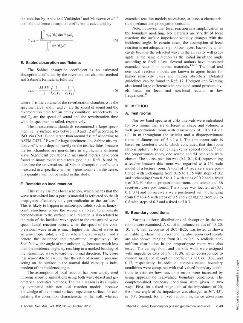
TABLE I. Errors for five uniform absorption conditions and one non-uniform condition in the proportionate room. The surface impedance, corresponding nor-
mal, random, field incidence coefficients, and Schroeder frequencies are indicated. The lowest errors are indicated in bold.
Mean e1 Mean e2
fnor anor arand afield fSch anor arand afield fnor anor arand afield fnor
BC1 40 0.10 0.17 0.18 566 4.0 2.2 2.1 1.8 2.2 0.6 0.6 0.9
BC2 20 0.18 0.30 0.32 423 3.7 1.4 1.4 1.2 2.4 0.6 0.6 0.9
BC3 10 0.33 0.49 0.52 331 3.7 1.2 1.1 1.0 2.5 0.9 0.9 1.0
BC4 7 0.43 0.60 0.65 299 3.7 1.4 1.3 1.0 2.6 1.1 1.2 1.1
BC5 4 0.64 0.79 0.83 260 3.5 1.8 1.7 1.2 2.6 1.7 1.9 1.7
Non-uniform 0.21 0.31 0.33 414 3.5 2.5 2.5 2.2 2.9 1.2 1.2 1.5
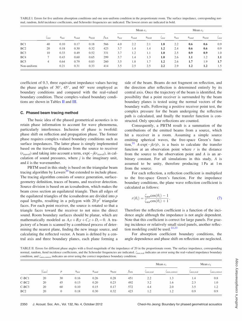
TABLE II. Errors for different phase angles with a fixed magnitude of the impedance of 20 in the proportionate room. The surface impedance, corresponding
normal, random, fiend incidence coefficients, and the Schroeder frequencies are indicated. fnor,real indicates an error using the real-valued impedance boundary
condition, and fnor,correct indicates an error using the correct impedance boundary condition.
Mean e1 Mean e2
jfnorj l anor arand afield fSch fnor,real fnor,correct fnor,real fnor,correct
C-BC1 20 30 0.16 0.26 0.28 451 2.2 1.3 1.4 0.8
C-BC2 20 45 0.13 0.20 0.23 492 3.2 1.6 2.3 1.0
C-BC3 20 60 0.10 0.15 0.17 572 4.4 2.0 3.5 1.2
BC2 20 0 0.18 0.30 0.32 423 1.2 1.2 0.9 0.9
2350 J. Acoust. Soc. Am., Vol. 132, No. 4, October 2012 Cheol-Ho Jeong: Boundary for phased geometrical acoustics
Au
tho
r's
com
plim
enta
ry c
op
y
Therefore a real-valued and positive reflection coefficient is
calculated as
ri ¼ffiffiffiffiffiffiffiffiffiffiffiffi1� ai
p; (8)
where the subscript i can be “nor,” “rand,” or “field.”
Challenges still remain in the phased beam tracing, par-
ticularly in considering diffraction and diffuse reflection.
Another problem of PBTM arises when beams intersect
more than one surface. If an intersecting polygon is detected,
there are two solutions: The original beam is followed by its
central axis ray4,20,22 or the original beam can be split.24,25
Beam-splitting algorithms possibly make simulations more
accurate, but they are computationally voracious.
For all PBTM simulations, 8000 beams were emitted
from the source, and they were traced up to the 100th reflec-
tion order. The reason for the large number of beams is due
to the fact that PBTM used does not incorporate a beam-
splitting algorithm when intersecting more than two surfa-
ces. In addition, a sufficient number of late reflections should
be calculated, therefore each beam was traced up to the
100th reflection order. For BC1, the average propagation dis-
tance for the 100th reflection order is 97 m, corresponding to
a sufficient decay range of 45 dB. For the other boundary
conditions, the decay ranges are even longer as the reverber-
ation times become shorter with increasing absorption.
D. Boundary element models
The boundary element method can solve acoustic
problems numerically based on the discretized Helmholtz–
Kirchhoff integral equation on a surface mesh.26 An in-
house boundary element model is used for comparisons. For
the proportionate room, the boundary element model con-
tains 6880 triangular elements with 3442 nodes of which the
6k per element condition is satisfied up to 1000 Hz. For the
disproportionate room, it has 7228 elements and 3616 nodes,
therefore its upper cutoff frequency is about 700 Hz. For the
two rooms, the linear shape function and seven Gaussian
points were used. The boundary element simulations are
regarded as the reference simulations.
E. Error measures
In predicting transfer functions using both PBTM and
BEM, the source is assumed to produce a sound pressure of
1 Pa at 1 m from the source in a free field. Once transfer
functions at 2 Hz intervals are calculated using PBTM and
BEM, they are converted to the dB scale re. 1 Pa, SPLPBTM
and SPLBEM, respectively. In addition, 1/3 octave band spec-
tra are computed based on the narrow band transfer func-
tions, and named as SPLPBTM,oct and SPLBEM,oct. Two errors
are defined to compare phased beam tracing simulations
with boundary element simulations: a narrow band error as
e1 by Eq. (9), and a 1/3 octave band error as e2 by Eq. (10)
e1ðfcÞ ¼1
Nline
Xfup
i¼flow
jSPLPBTMðiÞ � SPLBEMðiÞj ðdBÞ;
(9)
e2 ðfcÞ ¼ jSPLPBTM;octðfcÞ � SPLBEM;octðfcÞj ðdBÞ; (10)
where fup and flow are the upper and lower frequency limit of
a frequency band, fc is the center frequency of the band, and
Nline is the number of frequency lines in the frequency band
of interest. The upper valid frequencies of the proportionate
and disproportionate room boundary element models are
1000 and 700 Hz, respectively, therefore the highest center
frequencies of the 1/3 octave band are 800 Hz for the propor-
tionate room and 500 Hz for the disproportionate room. For
single-value errors, these errors are averaged over the entire
frequency range and over the receiver locations as shown in
Tables I–IV.
Two main sources of error in PBTM have been known:
errors at off-resonance frequencies due to geometrical trac-
ing and sphericity error.2,3 The former error influences e1
mainly for high impedances, whereas e2, which is based on
the sound pressure levels summed in 1/3 octave bands, is sel-
dom affected by the former error. However, the sphericity
error arises at very low frequencies for low surface imped-
ance. Because e2 is the 1/3 octave band error, which empha-
sizes low frequency errors more, the sphericity error can
increase e2 significantly. Therefore a larger e2 than e1 indi-
cates that the sphericity error prevails, whereas the opposite
holds for the error at off-resonance frequencies.
IV. RESULTS AND DISCUSSIONS
A. Uniform absorption in the proportionate room
Average simulation errors in the proportionate room are
shown in Table I and Figs. 1 and 2. In Table I, the frequency
and receiver averaged errors are listed, where it is found that
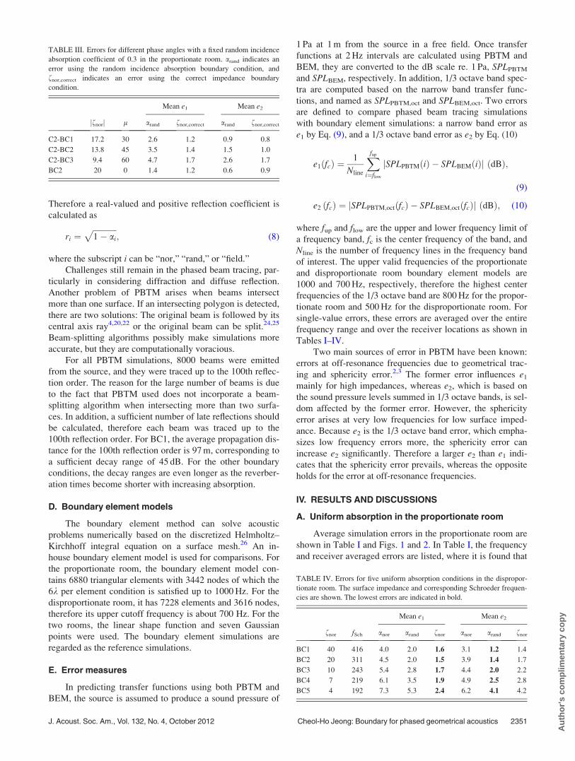
TABLE IV. Errors for five uniform absorption conditions in the dispropor-
tionate room. The surface impedance and corresponding Schroeder frequen-
cies are shown. The lowest errors are indicated in bold.
Mean e1 Mean e2
fnor fSch anor arand fnor anor arand fnor
BC1 40 416 4.0 2.0 1.6 3.1 1.2 1.4
BC2 20 311 4.5 2.0 1.5 3.9 1.4 1.7
BC3 10 243 5.4 2.8 1.7 4.4 2.0 2.2
BC4 7 219 6.1 3.5 1.9 4.9 2.5 2.8
BC5 4 192 7.3 5.3 2.4 6.2 4.1 4.2
TABLE III. Errors for different phase angles with a fixed random incidence
absorption coefficient of 0.3 in the proportionate room. arand indicates an
error using the random incidence absorption boundary condition, and
fnor,correct indicates an error using the correct impedance boundary
condition.
Mean e1 Mean e2
jfnorj l arand fnor,correct arand fnor,correct
C2-BC1 17.2 30 2.6 1.2 0.9 0.8
C2-BC2 13.8 45 3.5 1.4 1.5 1.0
C2-BC3 9.4 60 4.7 1.7 2.6 1.7
BC2 20 0 1.4 1.2 0.6 0.9
J. Acoust. Soc. Am., Vol. 132, No. 4, October 2012 Cheol-Ho Jeong: Boundary for phased geometrical acoustics 2351
Au
tho
r's
com
plim
enta
ry c
op
y
the errors using afield are only marginally different from the
errors using arand. This is mainly because these two absorp-
tion coefficients are very similar as shown in Table I, there-
fore the errors for arand, which is more widely used than
afield, are only shown in Figs. 1 and 2.
Figure 1 shows the averaged errors over the receiver
positions as a function of the frequency for anor, arand, and
fnor. For the lowest absorption case, BC1, the 1/3 octave
band error is significantly lower than the narrow band error.
For e1, the random incidence absorption boundary condition
shows best results below 200 Hz, whereas the impedance
boundary condition yields the best results at higher frequen-
cies. The errors are increased as the frequency increases. For
e2, the random incidence absorption and impedance bound-
ary conditions yields similar results at frequencies higher
than 300 Hz, whereas better agreements are found for the
random incidence absorption boundary condition below
300 Hz. The normal incidence absorption coefficient bound-
ary condition yields the worst results.
BC2 shows similar results to BC1. However, the errors
become lower than those for BC1, because the simulation
errors at the off-resonance frequencies become alleviated for
higher absorption cases.3 Among the three boundary condi-
tions (anor, arand, and fnor), the lowest e1 is found for the im-
pedance boundary condition, whereas the lowest e2 is
observed using the random incidence absorption in Table I.
This is mainly ascribed to the fact that the impedance
boundary condition slightly underestimates the room
response at frequencies below 300 Hz. Beyond the
Schroeder frequency of 423 Hz, the simulation accuracy
employing the impedance boundary is enhanced and at least
comparable to the random incidence absorption boundary
condition. Again, the normal incidence absorption coeffi-
cient boundary condition yields the worst results.
For BC3, the lowest e2 is found among the tested bound-
ary conditions in Table I. The impedance boundary condition
underestimates the room response at frequencies below
300 Hz, but the errors are reduced above the Schroeder
frequency. The best boundary condition in terms of e1 is the
impedance data, whereas a slightly better result is found for
the random incidence absorption boundary in terms of e2. At
frequencies lower than 60 Hz, the normal incidence absorp-
tion boundary produces the best results.
For BC4, increased errors are noticed for the random
incidence absorption and impedance boundary conditions at
low frequencies, whereas the normal incidence absorption
boundary condition yields the best result. Above 80 Hz, the
errors using the random incidence absorption and impedance
boundary conditions tend to be lower than those using the
normal incidence absorption coefficient, and the best corre-
spondence is found for the impedance boundary condition
above the Schroeder frequency.
For BC5, noticeably amplified errors are found at low
frequencies, whereas the high frequency errors are quite
FIG. 1. Errors averaged over the re-
ceiver positions as a function of fre-
quency in the proportionate room.
(a), (c), (e), (g), and (i) e1; (b), (d),
(f), (h), and (j) e2. (a) and (b) BC1;
(c) and (d) BC2; (e) and (f) BC3;
(g) and (h) BC4; (i) and (j) BC5.
anor; , arand; and
: fnor. � indicates the
Schroeder frequency.
2352 J. Acoust. Soc. Am., Vol. 132, No. 4, October 2012 Cheol-Ho Jeong: Boundary for phased geometrical acoustics
Au
tho
r's
com
plim
enta
ry c
op
y

reduced for the impedance and random incidence boundary
condition. The normal incidence absorption coefficient
boundary condition yields the lowest error at low frequen-
cies. Above 90 Hz, the errors using the random incidence
absorption and impedance boundary conditions become
lower, and the best correspondences are found for the imped-
ance boundary condition above the Schroeder frequency.
Note that e2 is larger than e1 for the impedance boundary
condition because large errors are found at low frequencies.
For the three low absorption cases (BC1–BC3), the ran-
dom incidence absorption boundary condition best approxi-
mates the local reaction boundary condition at low
frequencies. Above the Schroeder frequency, the impedance
boundary condition agrees best with the boundary element
simulations. e2 is smaller than e1 as can be seen in Table I;
this indicates that the errors at the resonance frequencies are
likely to be lower than those at the off-resonance frequencies
as also pointed out in Refs. 2 and 3. PBTM is inherently
more accurate at the resonance frequencies, therefore the
calculated 1/3 octave band spectra are more accurate. Gener-
ally the normal incidence absorption coefficient leads to the
most inaccurate simulations, whereas the random/field inci-
dence absorption and impedance boundary condition repre-
sent the locally reacting surfaces better. However, for the
first few axial modes below 100 Hz, the normal incidence
absorption boundary condition yields a similar agreement to
the other boundary conditions; this is not surprising because
it is obvious that the sound propagation is one dimensional.
Roughly speaking, below the Schroeder frequency, the
random incidence absorption boundary condition is better,
whereas the accurate results are guaranteed with the imped-
ance boundary condition above the Schroeder frequency.
The discrepancies between the random incidence absorption
and impedance boundary condition, however, are quite small
above the Schroeder frequency. For the very low absorption
case, the errors are increased as the frequency increases.
For the high absorption cases, the random incidence
absorption and impedance boundary conditions yield reliable
results at high frequencies, whereas the normal incidence
absorption produces the best results below 100 Hz. This is
related to the sphericity error for high absorptions at very
low frequencies as Lam and Ingard already pointed out2,27
because only the plane-wave reflection coefficient is
employed in the PBTM simulations. As Ingard found, the
sphericity error is indeed related to the angle of incidence:
The sphericity error for oblique angle incidence becomes
most significant for the lowest impedance, BC5, which sup-
ports the predominance of the incident energy at near normal
directions.27 This is the reason why the use of the normal
incidence absorption coefficient ensures accurate results in
this frequency range below 100 Hz. The best PBTM simula-
tion can be obtained by combining the boundary conditions:
the normal incidence absorption coefficient below 70 Hz, the
random incidence absorption between 70 and 150 Hz, and
the impedance beyond 150 Hz. However, this suggested
combination is specifically for this test room, and therefore
cannot be generalized. Because many room acoustic simula-
tions do not require responses in a very low frequency range,
FIG. 2. Errors averaged over the fre-
quency as a function of the source-to-
receiver distance in the proportionate
room. (a), (c), (e), (g), and (i) e1; (b),
(d), (f), (h), and (j) e2. (a) and
(b) BC1; (c) and (d) BC2; (e) and
(f) BC3; (g) and (h) BC4; (i) and (j)
BC5. , anor; , arand;
:fnor.
J. Acoust. Soc. Am., Vol. 132, No. 4, October 2012 Cheol-Ho Jeong: Boundary for phased geometrical acoustics 2353
Au
tho
r's
com
plim
enta
ry c
op
y
say below 100 Hz, the random incidence absorption, the field
incidence absorption, and impedance boundary conditions
are recommended in most cases.
Figure 2 shows the averaged error over the frequency as
a function of the source-and-receiver distance. Among the
boundary conditions, the normal incidence absorption
boundary condition yields the most inaccurate predictions,
while the random incidence absorption and impedance
boundary conditions produce small errors. The lowest e1 is
found using the impedance boundary condition. The random
incidence absorption boundary condition produces the low-
est e2 for the three lowest boundary conditions (BC1–BC3),
but both impedance and random incidence absorption bound-
ary conditions also produce the best results for BC4 and
BC5 as shown in Table II.
At some specific receiver locations, the errors are ampli-
fied. From Figs. 2(b), 2(d), 2(f), and 2(h), it is observed that
the 1/3 octave band error using the random incidence absorp-
tion boundary condition is less influenced by the receiver
position than using the impedance boundary condition. From
Fig. 2(j), large errors using the impedance boundary condi-
tion are found for specific receiver locations at (0.15, 1.0,
0.3), (0.15, 1.2, 0.3), (1.35, 0.2, 0.3), (1.55, 0.2, 0.3), and
(1.75, 0.2, 0.3). These receivers have a common aspect that
at least one of the first order reflections has a large incidence
angle. The largest incidence angles of the first order reflec-
tions for the listed five receivers are 73.7�, 77.0�, 76.2�,79.1�, and 78.8�, respectively. For such grazing incidence,
the plane wave reflection coefficient by Eq. (7) is known to
be incorrect and therefore yields large errors by using the im-
pedance boundary condition.23,28 To avoid such errors using
the impedance boundary condition that depend on the source
and receiver location, one may use the random incidence
absorption boundary condition.
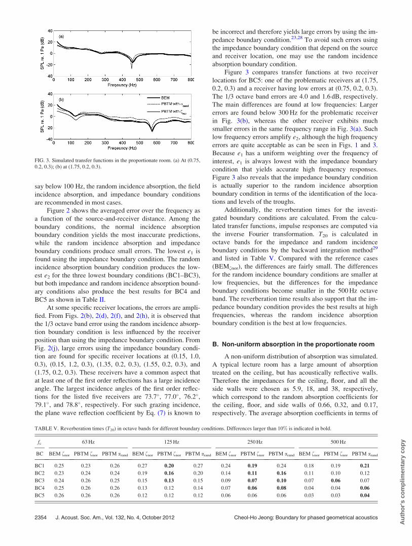
Figure 3 compares transfer functions at two receiver
locations for BC5: one of the problematic receivers at (1.75,
0.2, 0.3) and a receiver having low errors at (0.75, 0.2, 0.3).
The 1/3 octave band errors are 4.0 and 1.6 dB, respectively.
The main differences are found at low frequencies: Larger
errors are found below 300 Hz for the problematic receiver
in Fig. 3(b), whereas the other receiver exhibits much
smaller errors in the same frequency range in Fig. 3(a). Such
low frequency errors amplify e2, although the high frequency
errors are quite acceptable as can be seen in Figs. 1 and 3.
Because e1 has a uniform weighting over the frequency of
interest, e1 is always lowest with the impedance boundary
condition that yields accurate high frequency responses.
Figure 3 also reveals that the impedance boundary condition
is actually superior to the random incidence absorption
boundary condition in terms of the identification of the loca-
tions and levels of the troughs.
Additionally, the reverberation times for the investi-
gated boundary conditions are calculated. From the calcu-
lated transfer functions, impulse responses are computed via
the inverse Fourier transformation. T20 is calculated in
octave bands for the impedance and random incidence
boundary conditions by the backward integration method29
and listed in Table V. Compared with the reference cases
(BEMfnor), the differences are fairly small. The differences
for the random incidence boundary conditions are smaller at
low frequencies, but the differences for the impedance
boundary conditions become smaller in the 500 Hz octave
band. The reverberation time results also support that the im-
pedance boundary condition provides the best results at high
frequencies, whereas the random incidence absorption
boundary condition is the best at low frequencies.
B. Non-uniform absorption in the proportionate room
A non-uniform distribution of absorption was simulated.
A typical lecture room has a large amount of absorption
treated on the ceiling, but has acoustically reflective walls.
Therefore the impedances for the ceiling, floor, and all the
side walls were chosen as 5.9, 18, and 38, respectively,
which correspond to the random absorption coefficients for
the ceiling, floor, and side walls of 0.66, 0.32, and 0.17,
respectively. The average absorption coefficients in terms of
FIG. 3. Simulated transfer functions in the proportionate room. (a) At (0.75,
0.2, 0.3); (b) at (1.75, 0.2, 0.3).
TABLE V. Reverberation times (T20) in octave bands for different boundary conditions. Differences larger than 10% is indicated in bold.
fc 63 Hz 125 Hz 250 Hz 500 Hz
BC BEM fnor PBTM fnor PBTM arand BEM fnor PBTM fnor PBTM arand BEM fnor PBTM fnor PBTM arand BEM fnor PBTM fnor PBTM arand
BC1 0.25 0.23 0.26 0.27 0.20 0.27 0.24 0.19 0.24 0.18 0.19 0.21
BC2 0.23 0.24 0.24 0.19 0.16 0.20 0.14 0.11 0.16 0.11 0.10 0.12
BC3 0.24 0.26 0.25 0.15 0.13 0.15 0.09 0.07 0.10 0.07 0.06 0.07
BC4 0.25 0.26 0.26 0.13 0.12 0.14 0.07 0.06 0.08 0.04 0.04 0.06
BC5 0.26 0.26 0.26 0.12 0.12 0.12 0.06 0.06 0.06 0.03 0.03 0.04
2354 J. Acoust. Soc. Am., Vol. 132, No. 4, October 2012 Cheol-Ho Jeong: Boundary for phased geometrical acoustics
Au
tho
r's
com
plim
enta
ry c
op
y
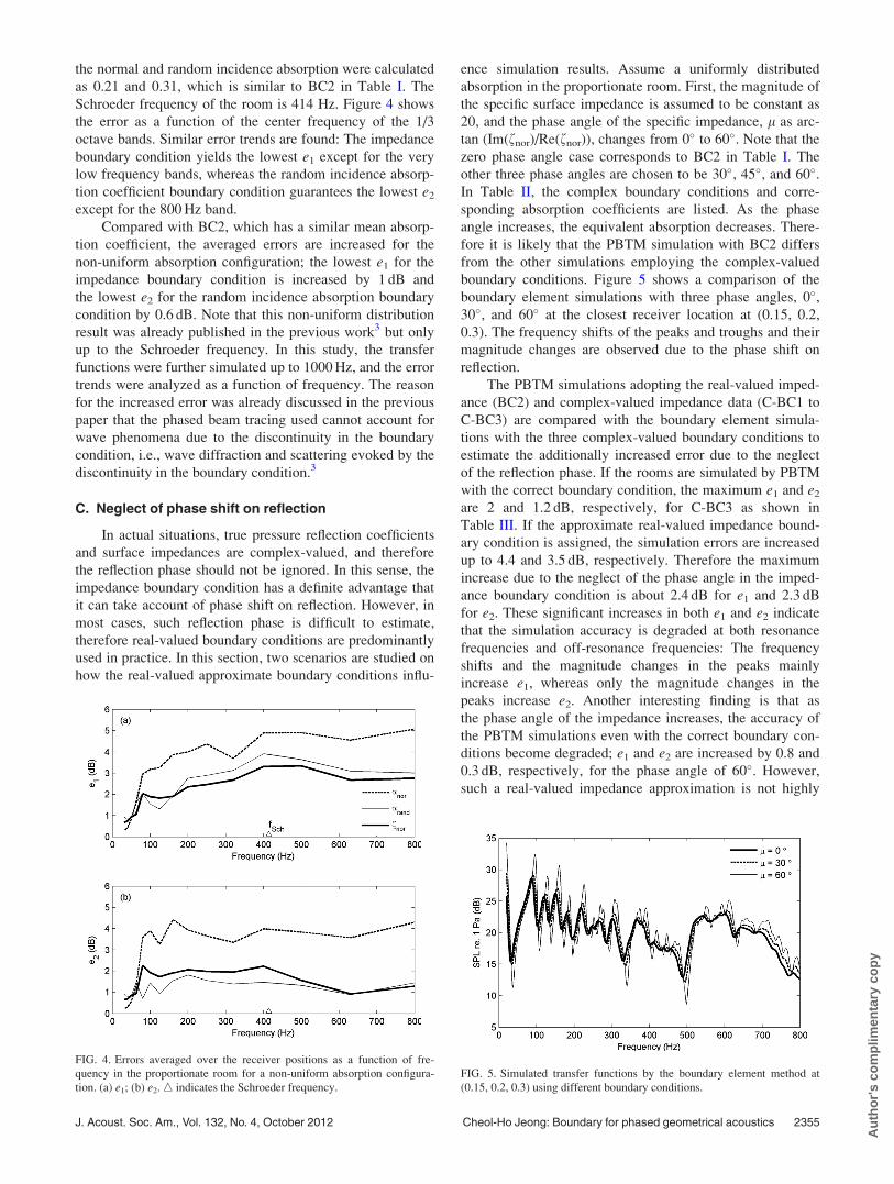
the normal and random incidence absorption were calculated
as 0.21 and 0.31, which is similar to BC2 in Table I. The
Schroeder frequency of the room is 414 Hz. Figure 4 shows
the error as a function of the center frequency of the 1/3
octave bands. Similar error trends are found: The impedance
boundary condition yields the lowest e1 except for the very
low frequency bands, whereas the random incidence absorp-
tion coefficient boundary condition guarantees the lowest e2
except for the 800 Hz band.
Compared with BC2, which has a similar mean absorp-
tion coefficient, the averaged errors are increased for the
non-uniform absorption configuration; the lowest e1 for the
impedance boundary condition is increased by 1 dB and
the lowest e2 for the random incidence absorption boundary
condition by 0.6 dB. Note that this non-uniform distribution
result was already published in the previous work3 but only
up to the Schroeder frequency. In this study, the transfer
functions were further simulated up to 1000 Hz, and the error
trends were analyzed as a function of frequency. The reason
for the increased error was already discussed in the previous
paper that the phased beam tracing used cannot account for
wave phenomena due to the discontinuity in the boundary
condition, i.e., wave diffraction and scattering evoked by the
discontinuity in the boundary condition.3
C. Neglect of phase shift on reflection
In actual situations, true pressure reflection coefficients
and surface impedances are complex-valued, and therefore
the reflection phase should not be ignored. In this sense, the
impedance boundary condition has a definite advantage that
it can take account of phase shift on reflection. However, in
most cases, such reflection phase is difficult to estimate,
therefore real-valued boundary conditions are predominantly
used in practice. In this section, two scenarios are studied on
how the real-valued approximate boundary conditions influ-
ence simulation results. Assume a uniformly distributed
absorption in the proportionate room. First, the magnitude of
the specific surface impedance is assumed to be constant as
20, and the phase angle of the specific impedance, l as arc-
tan (Im(fnor)/Re(fnor)), changes from 0� to 60�. Note that the
zero phase angle case corresponds to BC2 in Table I. The
other three phase angles are chosen to be 30�, 45�, and 60�.In Table II, the complex boundary conditions and corre-
sponding absorption coefficients are listed. As the phase
angle increases, the equivalent absorption decreases. There-
fore it is likely that the PBTM simulation with BC2 differs
from the other simulations employing the complex-valued
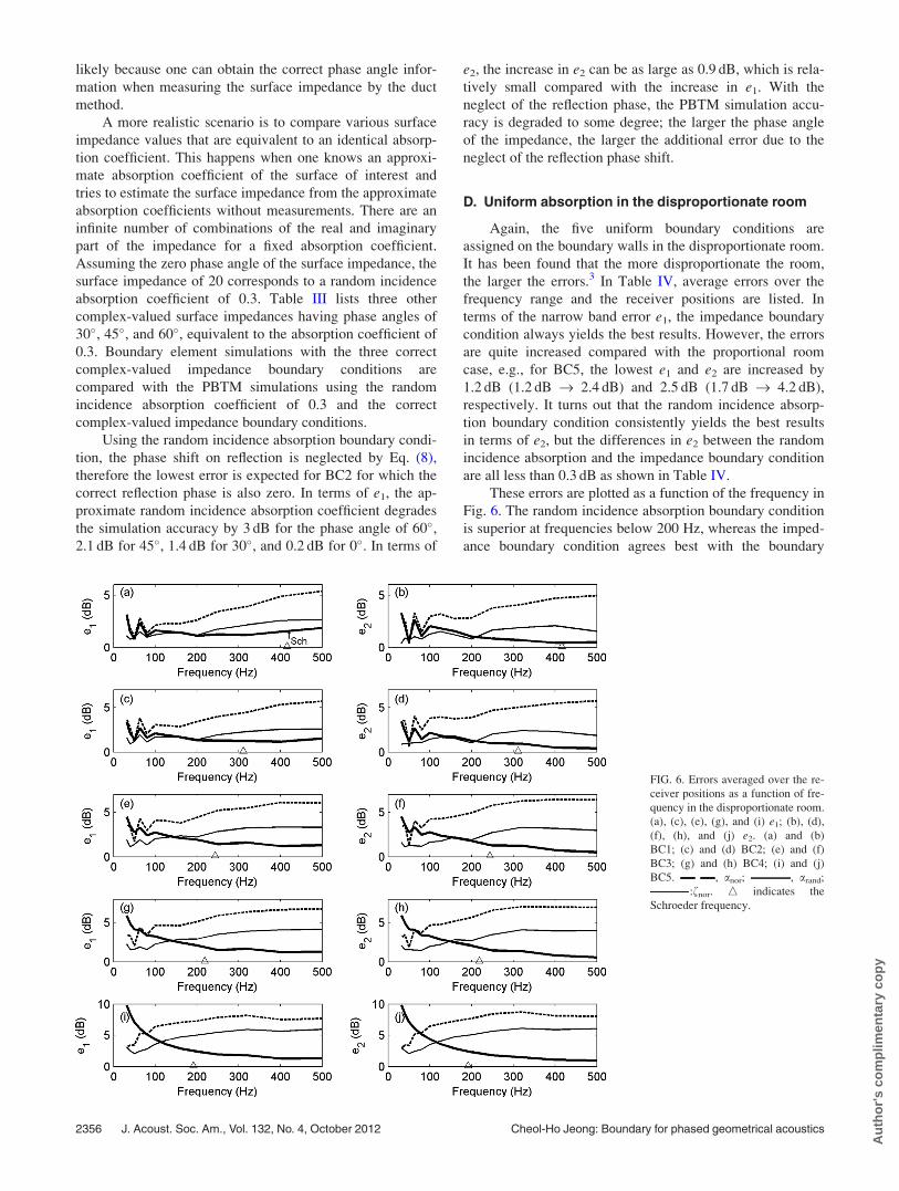
boundary conditions. Figure 5 shows a comparison of the
boundary element simulations with three phase angles, 0�,30�, and 60� at the closest receiver location at (0.15, 0.2,
0.3). The frequency shifts of the peaks and troughs and their
magnitude changes are observed due to the phase shift on
reflection.
The PBTM simulations adopting the real-valued imped-
ance (BC2) and complex-valued impedance data (C-BC1 to
C-BC3) are compared with the boundary element simula-
tions with the three complex-valued boundary conditions to
estimate the additionally increased error due to the neglect
of the reflection phase. If the rooms are simulated by PBTM
with the correct boundary condition, the maximum e1 and e2
are 2 and 1.2 dB, respectively, for C-BC3 as shown in
Table III. If the approximate real-valued impedance bound-
ary condition is assigned, the simulation errors are increased
up to 4.4 and 3.5 dB, respectively. Therefore the maximum
increase due to the neglect of the phase angle in the imped-
ance boundary condition is about 2.4 dB for e1 and 2.3 dB
for e2. These significant increases in both e1 and e2 indicate
that the simulation accuracy is degraded at both resonance
frequencies and off-resonance frequencies: The frequency
shifts and the magnitude changes in the peaks mainly
increase e1, whereas only the magnitude changes in the
peaks increase e2. Another interesting finding is that as
the phase angle of the impedance increases, the accuracy of
the PBTM simulations even with the correct boundary con-
ditions become degraded; e1 and e2 are increased by 0.8 and
0.3 dB, respectively, for the phase angle of 60�. However,
such a real-valued impedance approximation is not highly
FIG. 5. Simulated transfer functions by the boundary element method at
(0.15, 0.2, 0.3) using different boundary conditions.
FIG. 4. Errors averaged over the receiver positions as a function of fre-
quency in the proportionate room for a non-uniform absorption configura-
tion. (a) e1; (b) e2. � indicates the Schroeder frequency.
J. Acoust. Soc. Am., Vol. 132, No. 4, October 2012 Cheol-Ho Jeong: Boundary for phased geometrical acoustics 2355
Au
tho
r's
com
plim
enta
ry c
op
y
likely because one can obtain the correct phase angle infor-
mation when measuring the surface impedance by the duct
method.
A more realistic scenario is to compare various surface
impedance values that are equivalent to an identical absorp-
tion coefficient. This happens when one knows an approxi-
mate absorption coefficient of the surface of interest and
tries to estimate the surface impedance from the approximate
absorption coefficients without measurements. There are an
infinite number of combinations of the real and imaginary
part of the impedance for a fixed absorption coefficient.
Assuming the zero phase angle of the surface impedance, the
surface impedance of 20 corresponds to a random incidence
absorption coefficient of 0.3. Table III lists three other
complex-valued surface impedances having phase angles of
30�, 45�, and 60�, equivalent to the absorption coefficient of
0.3. Boundary element simulations with the three correct
complex-valued impedance boundary conditions are
compared with the PBTM simulations using the random
incidence absorption coefficient of 0.3 and the correct
complex-valued impedance boundary conditions.
Using the random incidence absorption boundary condi-
tion, the phase shift on reflection is neglected by Eq. (8),
therefore the lowest error is expected for BC2 for which the
correct reflection phase is also zero. In terms of e1, the ap-
proximate random incidence absorption coefficient degrades
the simulation accuracy by 3 dB for the phase angle of 60�,2.1 dB for 45�, 1.4 dB for 30�, and 0.2 dB for 0�. In terms of
e2, the increase in e2 can be as large as 0.9 dB, which is rela-
tively small compared with the increase in e1. With the
neglect of the reflection phase, the PBTM simulation accu-
racy is degraded to some degree; the larger the phase angle
of the impedance, the larger the additional error due to the
neglect of the reflection phase shift.
D. Uniform absorption in the disproportionate room
Again, the five uniform boundary conditions are
assigned on the boundary walls in the disproportionate room.
It has been found that the more disproportionate the room,
the larger the errors.3 In Table IV, average errors over the
frequency range and the receiver positions are listed. In
terms of the narrow band error e1, the impedance boundary
condition always yields the best results. However, the errors
are quite increased compared with the proportional room
case, e.g., for BC5, the lowest e1 and e2 are increased by
1.2 dB (1.2 dB fi 2.4 dB) and 2.5 dB (1.7 dB fi 4.2 dB),
respectively. It turns out that the random incidence absorp-
tion boundary condition consistently yields the best results
in terms of e2, but the differences in e2 between the random
incidence absorption and the impedance boundary condition
are all less than 0.3 dB as shown in Table IV.
These errors are plotted as a function of the frequency in
Fig. 6. The random incidence absorption boundary condition
is superior at frequencies below 200 Hz, whereas the imped-
ance boundary condition agrees best with the boundary
FIG. 6. Errors averaged over the re-
ceiver positions as a function of fre-
quency in the disproportionate room.
(a), (c), (e), (g), and (i) e1; (b), (d),
(f), (h), and (j) e2. (a) and (b)
BC1; (c) and (d) BC2; (e) and (f)
BC3; (g) and (h) BC4; (i) and (j)
BC5. , anor; , arand;
:fnor. � indicates the
Schroeder frequency.
2356 J. Acoust. Soc. Am., Vol. 132, No. 4, October 2012 Cheol-Ho Jeong: Boundary for phased geometrical acoustics
Au
tho
r's
com
plim
enta
ry c
op
y
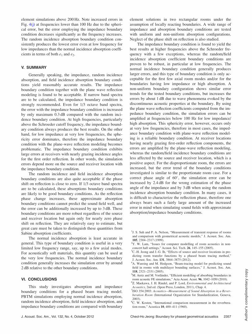
element simulations above 200 Hz. Note increased errors in
Fig. 4(j) at frequencies lower than 100 Hz due to the spheri-
cal error, but the error employing the impedance boundary
condition decreases significantly as the frequency increases.
The random incidence absorption boundary condition con-
sistently produces the lowest error even at low frequency for
low impedances than the normal incidence absorption coeffi-
cients in terms of both e1 and e2.
V. SUMMARY
Generally speaking, the impedance, random incidence
absorption, and field incidence absorption boundary condi-
tions yield reasonably accurate results. The impedance
boundary condition together with the plane wave reflection
modeling is found to be acceptable. If narrow band spectra
are to be calculated, the impedance boundary condition is
strongly recommended. Even for 1/3 octave band spectra,
the error with the impedance boundary condition is increased
by only maximum 0.3 dB compared with the random inci-
dence boundary condition. At high frequencies, particularly
above the Schroeder cutoff frequency, the impedance bound-
ary condition always produces the best results. On the other
hand, for low impedance at very low frequencies, the sphe-
ricity error dominates, therefore the impedance boundary
condition with the plane-wave reflection modeling becomes
problematic. The impedance boundary condition exhibits
large errors at receivers with nearly grazing incidence angles
for the first order reflection. In other words, the simulation
errors depend more on the source and receiver location with
the impedance boundary condition.
The random incidence and field incidence absorption
boundary conditions are also quite acceptable if the phase
shift on reflection is close to zero. If 1/3 octave band spectra
are to be calculated, these absorptions boundary conditions
are likely to be good boundary conditions. As the reflection
phase change increases, these approximate absorption
boundary conditions cannot predict the sound field well, and
the error can be additionally increased by up to 3 dB. These
boundary conditions are more robust regardless of the source
and receiver location but again only for nearly zero phase
shift on reflection. They are relatively easy to estimate, but
great care must be taken to distinguish these quantities from
Sabine absorption coefficients.
The normal incidence absorption is least accurate in
general. This type of boundary condition is useful in a very
limited low frequency range, say, up to a few axial modes.
For acoustically soft materials, this quantity can be used at
the very low frequencies. The normal incidence boundary
condition generally increases the simulation error by around
2 dB relative to the other boundary conditions.
VI. CONCLUSIONS
This study investigates absorption and impedance
boundary conditions for a phased beam tracing model.
PBTM simulations employing normal incidence absorption,
random incidence absorption, field incidence absorption, and
impedance boundary conditions are compared with boundary
element solutions in two rectangular rooms under the
assumption of locally reacting boundaries. A wide range of
impedance and absorption boundary conditions are tested
with uniform and non-uniform absorption configurations.
Neglect of the phase shift on reflection is also studied.
The impedance boundary condition is found to yield the
best results at higher frequencies above the Schroeder fre-
quency with a few exceptions, whereas the random/field
incidence absorption coefficient boundary conditions are
proven to be robust, in particular at low frequencies. The
normal incidence boundary condition generally produces
larger errors, and this type of boundary condition is only ac-
ceptable for the first few axial room modes and/or for the
boundaries having low impedance or high absorption. A
non-uniform boundary configuration shows similar error
trends for the tested boundary conditions, but increases the
errors by about 1 dB due to wave phenomena evoked by the
discontinuous acoustic properties at the boundary. By using
the plane wave reflection coefficients computed from the im-
pedance boundary condition, the simulation errors can be
amplified at frequencies below 100 Hz for low impedance/
high absorption. This sphericity error, however, occurs only
at very low frequencies, therefore in most cases, the imped-
ance boundary condition with plane-wave reflection model-
ing is a reliable boundary condition. At receiver locations
having nearly grazing first-order reflection components, the
errors are amplified by the plane-wave reflection modeling,
whereas the random/field incidence boundary conditions are
less affected by the source and receiver location, which is a
positive aspect. For the disproportionate room, the errors are
increased, but the error trend of the boundary conditions
investigated is similar to the proportionate room case. For a
correct phase angle of 60�, the simulation error can be
increased by 2.4 dB for the wrong estimation of the phase
angle of the impedance and by 3 dB when using the random
incidence absorption boundary condition. In many cases, it
is difficult to characterize the reflection phase, therefore one
always bears such a fairly large amount of the increased
error in mind when simulating sound fields with approximate
absorption/impedance boundary conditions.
1J. S. Suh and P. A. Nelson, “Measurement of transient response of rooms
and comparison with geometrical acoustic models,” J. Acoust. Soc. Am.
105, 2304–2317 (1999).2Y. W. Lam, “Issues for computer modelling of room acoustics in non-
concert hall settings,” Acoust. Sci. Tech. 26, 145–155 (2005).3C.-H. Jeong and J.-G. Ih, “Effects of source and receiver locations in pre-
dicting room transfer functions by a phased beam tracing method,”
J. Acoust. Soc. Am. 131, 3864–3875 (2012).4A. Wareing and M. Hodgson, “Beam-tracing model for predicting sound
field in rooms with multilayer bounding surfaces,” J. Acoust. Soc. Am.
118, 2321–2331 (2005).5M. Aretz and M. Vorl€ander, “Efficient modelling of absorbing boundaries in
room acoustic FE simulations,” Acta Acust. Acust. 96, 1042–1050 (2010).6Z. Maekawa, J. H. Rindel, and P. Lord, Environmental and ArchitecturalAcoustics, 2nd ed. (Spon Press, London, 2011), Chap. 4.
7ISO 354:2003: Acoustics—Measurement of Sound Absorption in a Rever-beration Room (International Organization for Standardization, Geneva,
2003).8C. W. Kosten, “International comparison measurement in the reverbera-
tion room,” Acustica 10, 400–411 (1960).
J. Acoust. Soc. Am., Vol. 132, No. 4, October 2012 Cheol-Ho Jeong: Boundary for phased geometrical acoustics 2357
Au
tho
r's
com
plim
enta
ry c
op
y
9M. Vercammen, “Improving the accuracy of sound absorption measure-
ment according to ISO 354,” Proceedings of the International Symposiumon Room Acoustics, Melbourne, Australia (2010).
10H. Kuttruff, Room Acoustics, 4th ed. (Spon Press, London, 2000), Chap.
2.5.11ASTM C423:2009: Standard Test Method for Sound Absorption and
Sound Absorption Coefficients by the Reverberation Room Method (Amer-
ican Society for Testing and Materials International, West Conshohocken,
PA, 2009).12K. Attenborough, “Acoustical characteristics of porous materials,” Phys.
Rep. 82, 179–227 (1982).13C. Klein and A. Cops, “Angle dependence of impedance of a porous
layer,” Acustica 44, 258–264 (1980).14D. B. Bliss and S. E. Burke, “Experimental investigation of the bulk reac-
tion boundary condition,” J. Acoust. Soc. Am. 71, 546–551 (1982).15D. J. Sides and K. J. Mulholland, “The variation of normal layer imped-
ance with angle of incidence,” J. Sound Vib. 14, 139–142 (1971).16E. A. G. Shaw, “The acoustic wave guide. II. Some specific normal acoustic
impedance measurements of typical porous surfaces with respect of normally
and obliquely incident waves,” J. Acoust. Soc. Am. 25, 231–235 (1953).17C.-H. Jeong, “Guideline for adopting the local reaction assumption for po-
rous absorbers in terms of random incidence absorption coefficients,” Acta
Acust. Acust. 97, 779–790 (2011).18M. Hodgson, and A. Wareing, “Comparisons of predicted steady-state lev-
els in rooms with extended- and local-reaction bounding surfaces,”
J. Sound Vib. 309, 167–177 (2008).
19M. M. Louden, “Dimension ratios of rectangular rooms with good distri-
bution of eigentones,” Acustica 24, 101–104 (1971).20T. Lewers, “A combined beam tracing and radiant exchange computer-
model of room acoustics,” Appl. Acoust. 38, 161–178 (1993).21P. M. Morse and K. U. Ingard, Theoretical Acoustics (McGraw-Hill, New
York, 1968), p. 319.22C.-H. Jeong, J.-G. Ih, and J. H. Rindel, “An approximate treatment of reflection
coefficient in the phased beam tracing method for the simulation of enclosed
sound fields at medium frequencies,” Appl. Acoust. 69, 601–613 (2007).23J. H. Rindel, “Modeling the angle-dependent pressure reflection factor,”
Appl. Acoust. 38, 223–234 (1993).24T. Funkhouser, N. Tsingos, I. Carlbom, G. Elko, M. Sondhi, J. E. West, G.
Pingali, P. Min, and A. Ngan, “A beam tracing method for interactive ar-
chitectural acoustics,” J. Acoust. Soc. Am. 115, 739–756 (2004).25I. A. Drumm, and Y. W. Lam, “The adaptive beam-tracing algorithm,”
J. Acoust. Soc. Am. 107, 1405–1412 (2000).26M. Vorlander, Auralization: Fundamentals of Acoustics, Modelling, Simu-
lation, Algorithms and Acoustic Virtual Reality (Springer-Verlag, Berlin,
2008), pp. 155–156.27U. Ingard, “On the reflection of a spherical sound wave from an infinite
plane,” J. Acoust. Soc. Am. 23, 329–335 (1951).28S.-I. Thomasson, “Theory and experiments on the sound absorption as
function of the area,” Report TRITA-TAK8201, KTH, Stockholm, Swe-
den (1982).29M. R. Schroeder, “New method of measuring reverberation time,”
J. Acoust. Soc. Am. 37, 409–412 (1965).
2358 J. Acoust. Soc. Am., Vol. 132, No. 4, October 2012 Cheol-Ho Jeong: Boundary for phased geometrical acoustics
Au
tho
r's
com
plim
enta
ry c
op
y