absolute extreme values are either maximum or minimum points on a curve. they are sometimes called...
TRANSCRIPT
Absolute extreme values are either maximum or minimum points on a curve.
They are sometimes called global extremes.
They are also sometimes called absolute extrema.(Extrema is the plural of the Latin extremum.)
4.1 Extreme Values of Functions
4.1 Extreme Values of Functions
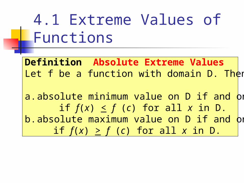
Definition Absolute Extreme ValuesLet f be a function with domain D. Then f (c) is the
a. absolute minimum value on D if and only if f(x) < f (c) for all x in D.b. absolute maximum value on D if and only if f(x) > f (c) for all x in D.
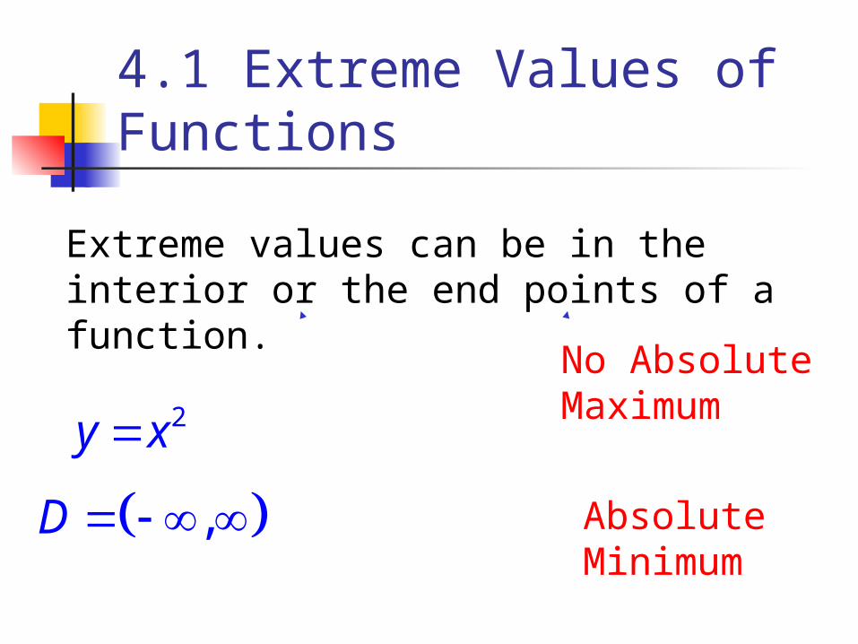
Extreme values can be in the interior or the end points of a function.
2y x
,D Absolute Minimum
No AbsoluteMaximum
4.1 Extreme Values of Functions
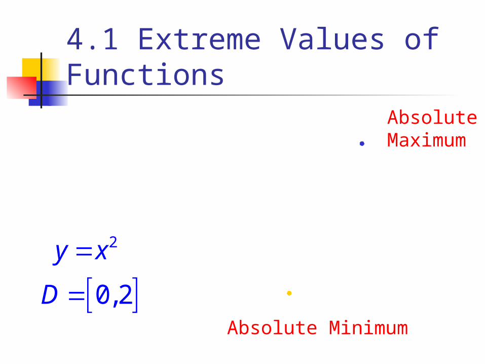
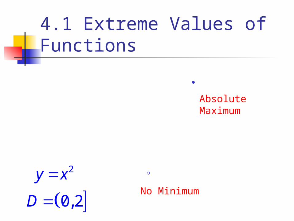
2y x
0,2D Absolute Minimum
AbsoluteMaximum
4.1 Extreme Values of Functions
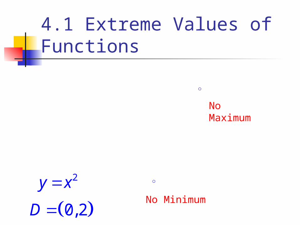
2y x
0,2D No Minimum
AbsoluteMaximum
4.1 Extreme Values of Functions
2y x
0,2D No Minimum
NoMaximum
4.1 Extreme Values of Functions
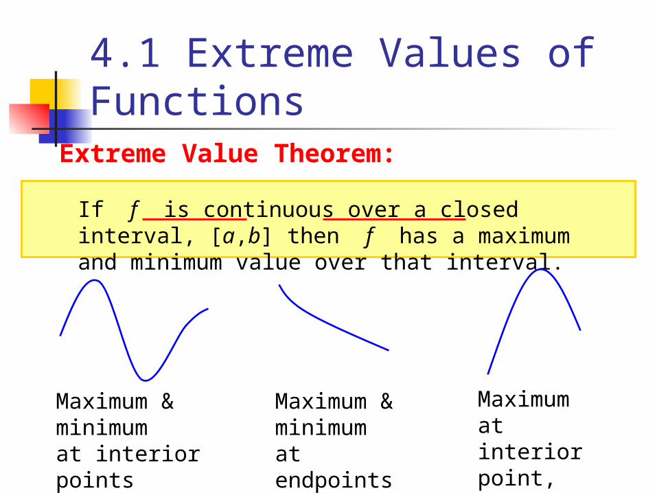
Extreme Value Theorem:
If f is continuous over a closed interval, [a,b] then f has a maximum and minimum value over that interval.
Maximum & minimumat interior points
Maximum & minimumat endpoints
Maximum at interior point, minimum at endpoint
4.1 Extreme Values of Functions
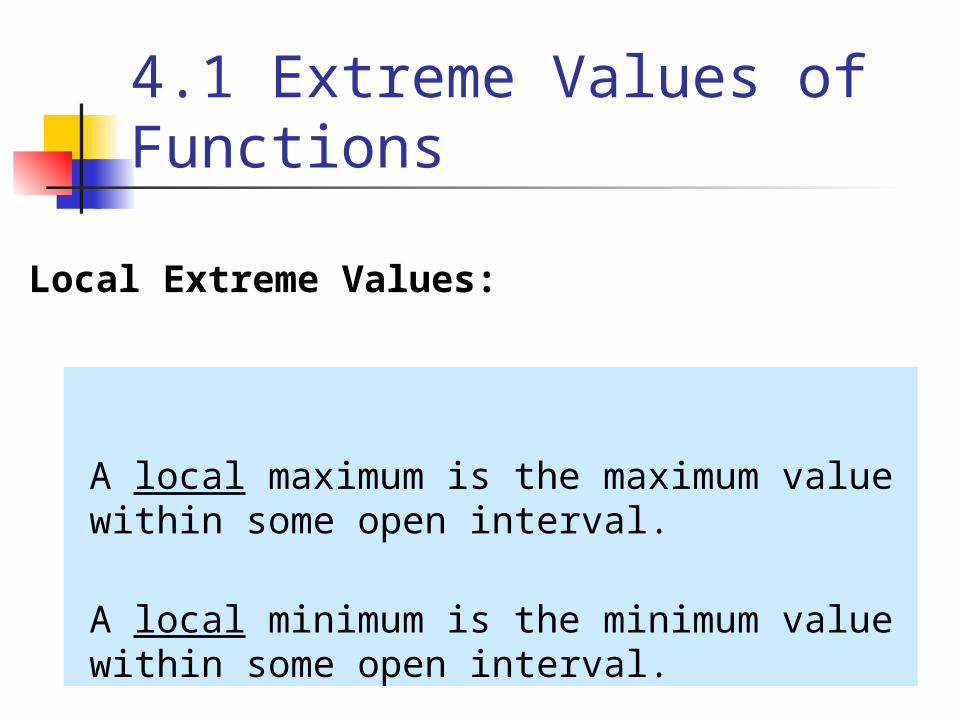
Local Extreme Values:
A local maximum is the maximum value within some open interval.
A local minimum is the minimum value within some open interval.
4.1 Extreme Values of Functions
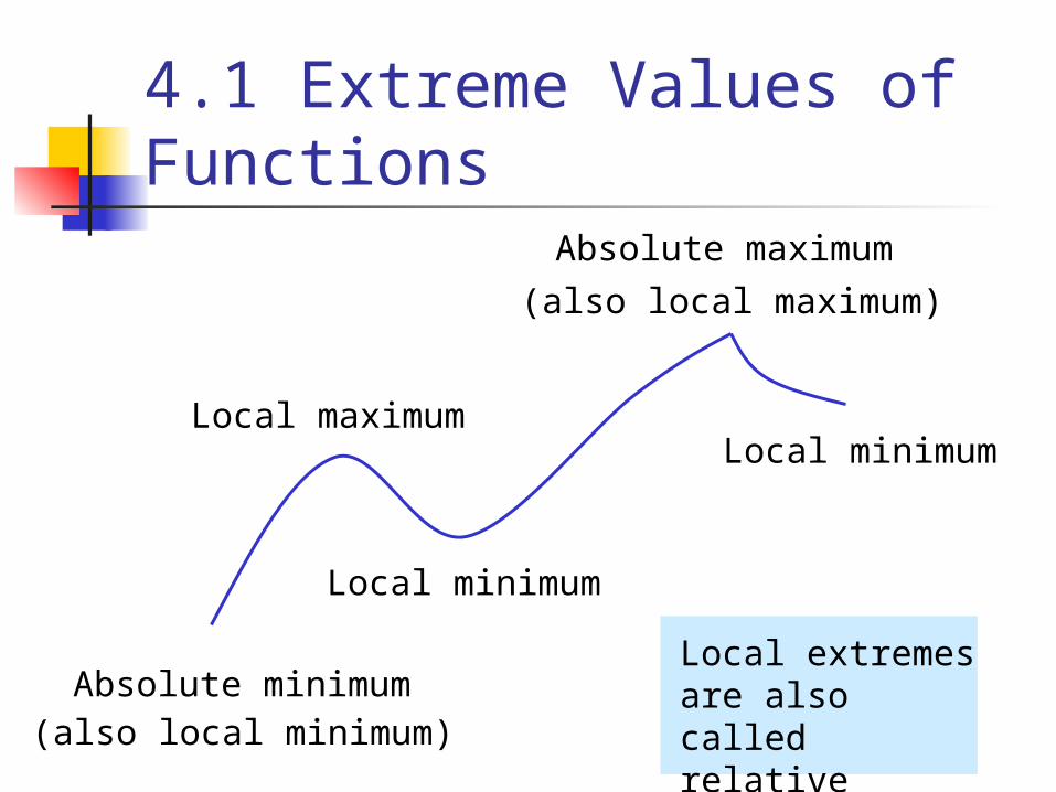
Absolute minimum(also local minimum)
Local maximum
Local minimum
Absolute maximum
(also local maximum)
Local minimum
Local extremes are also called relative extremes.
4.1 Extreme Values of Functions
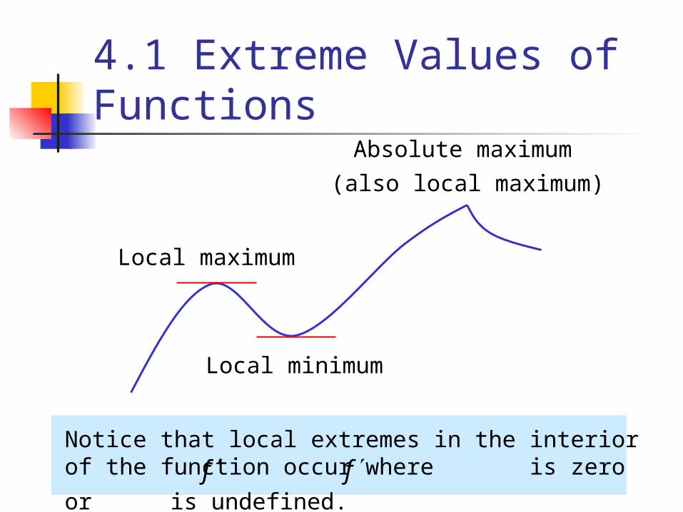
Local maximum
Local minimum
Notice that local extremes in the interior of the function
occur where is zero or is undefined.f f
Absolute maximum
(also local maximum)
4.1 Extreme Values of Functions
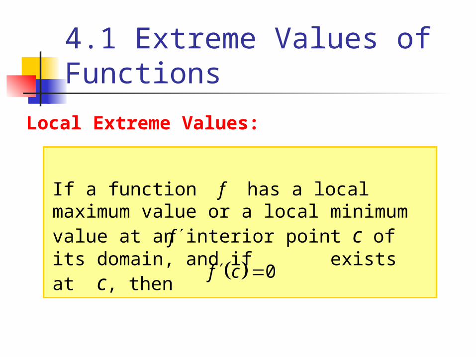
Local Extreme Values:
If a function f has a local maximum value or a local minimum value at an interior point c of its domain, and if exists at c, then
0f c
f
4.1 Extreme Values of Functions
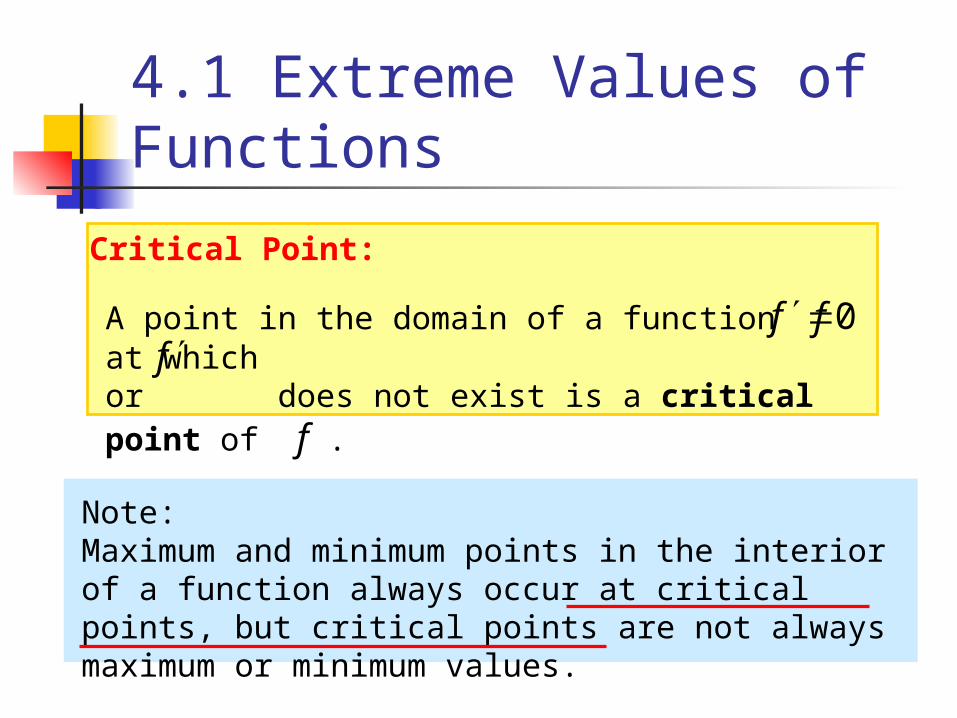
Critical Point:
A point in the domain of a function f at which
or does not exist is a critical point of f .0f
f
Note:Maximum and minimum points in the interior of a function always occur at critical points, but critical points are not always maximum or minimum values.
4.1 Extreme Values of Functions
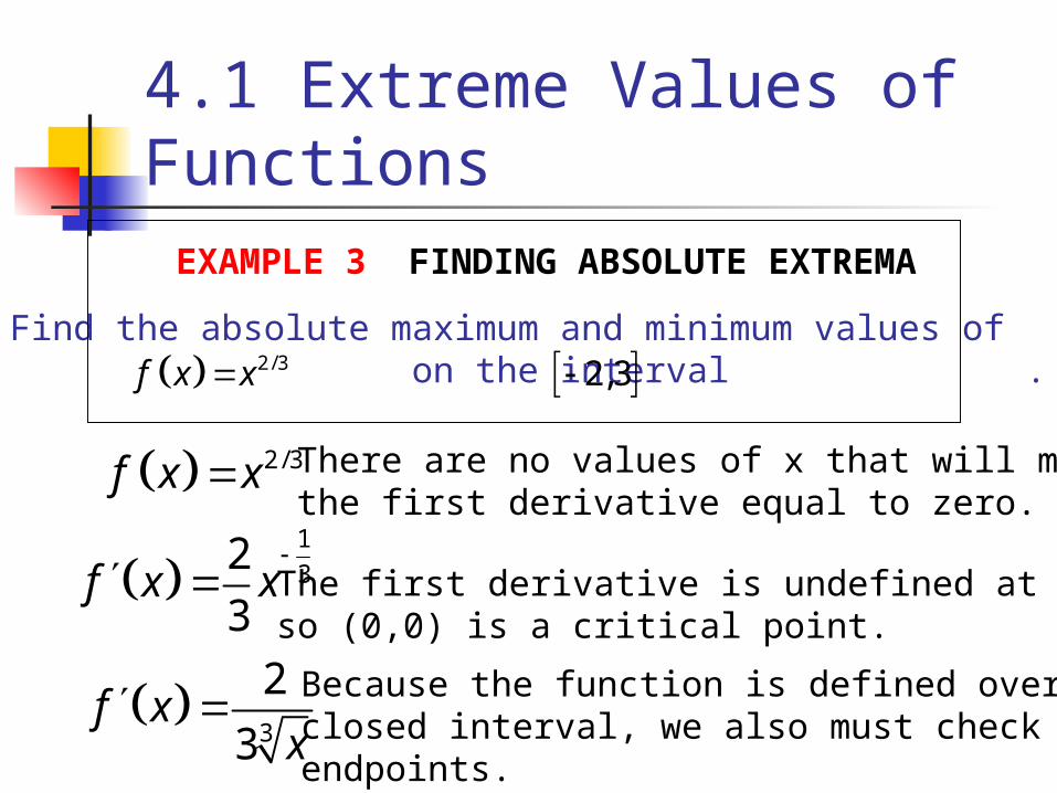
EXAMPLE 3 FINDING ABSOLUTE EXTREMA
Find the absolute maximum and minimum values of on the interval . 2/3f x x 2,3
2/3f x x
1
32
3f x x
3
2
3f x
x
There are no values of x that will makethe first derivative equal to zero.
The first derivative is undefined at x=0,so (0,0) is a critical point.
Because the function is defined over aclosed interval, we also must check theendpoints.
4.1 Extreme Values of Functions
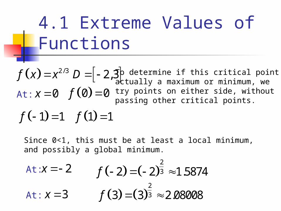
0 0f
To determine if this critical point isactually a maximum or minimum, wetry points on either side, withoutpassing other critical points.
2/3f x x
1 1f 1 1f
Since 0<1, this must be at least a local minimum, and possibly a global minimum.
2,3D
At: 0x
At: 2x 2
32 2 1.5874f
At: 3x 2
33 3 2.08008f
4.1 Extreme Values of Functions
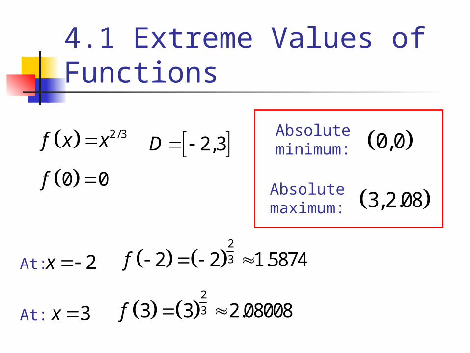
0 0f
2/3f x x 2,3D
At: 2x 2
32 2 1.5874f
At: 3x
Absoluteminimum:
Absolutemaximum:
0,0
3,2.08
2
33 3 2.08008f
4.1 Extreme Values of Functions
4.1 Extreme Values of Functions
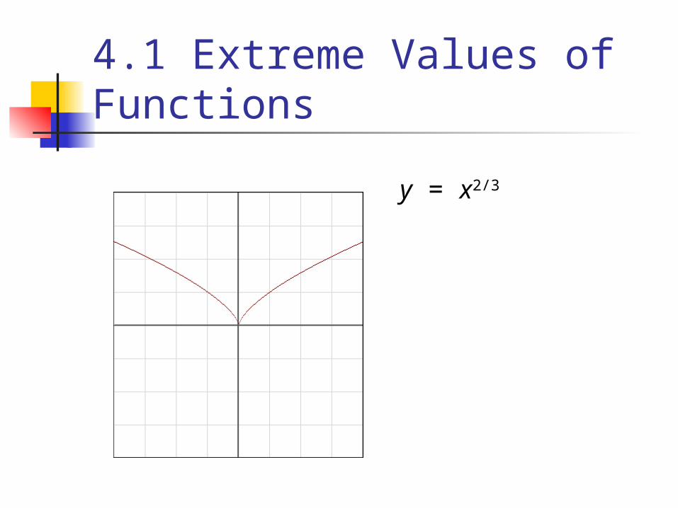
y = x2/3
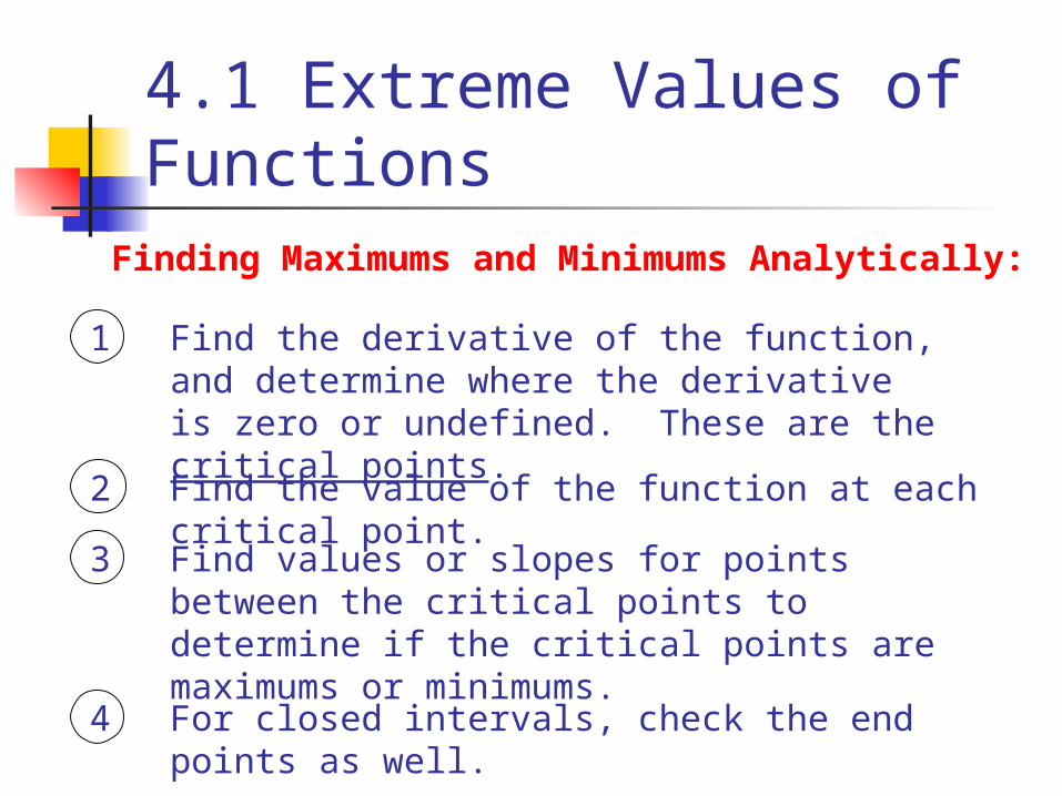
Finding Maximums and Minimums Analytically:
1 Find the derivative of the function, and determine where the derivative is zero or undefined. These are the critical points.
2 Find the value of the function at each critical point.
3 Find values or slopes for points between the critical points to determine if the critical points are maximums or minimums.
4 For closed intervals, check the end points as well.
4.1 Extreme Values of Functions
4.1 Extreme Values of Functions
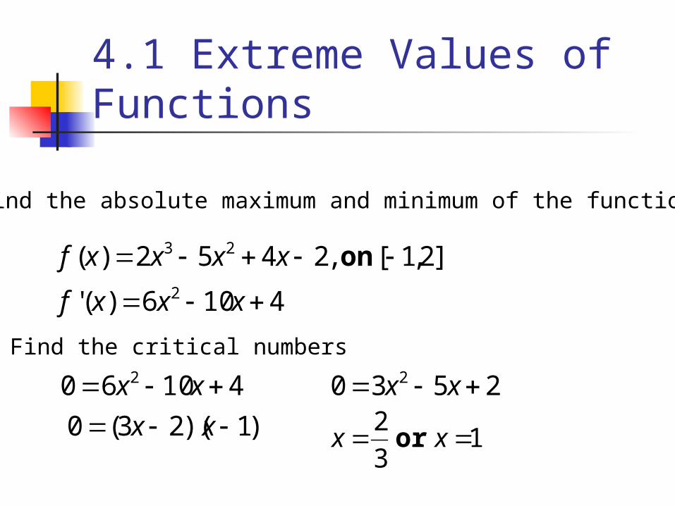
Find the absolute maximum and minimum of the function
]2,1[,2452)( 23 onxxxxf
4106)(' 2 xxxf
41060 2 xx
Find the critical numbers
2530 2 xx
)1)(23(0 xx 13
2 xx or
4.1 Extreme Values of Functions
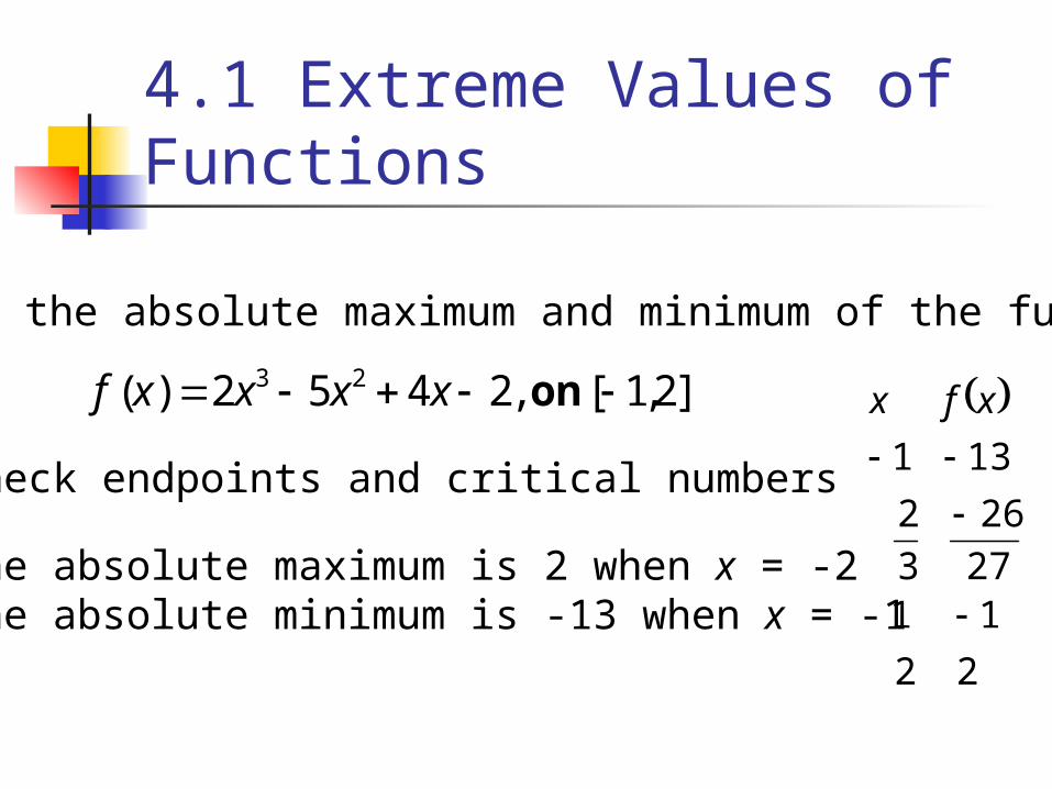
Find the absolute maximum and minimum of the function
]2,1[,2452)( 23 onxxxxf
Check endpoints and critical numbers
The absolute maximum is 2 when x = -2The absolute minimum is -13 when x = -1
22
1127
26
3
2
131
xfx
4.1 Extreme Values of Functions
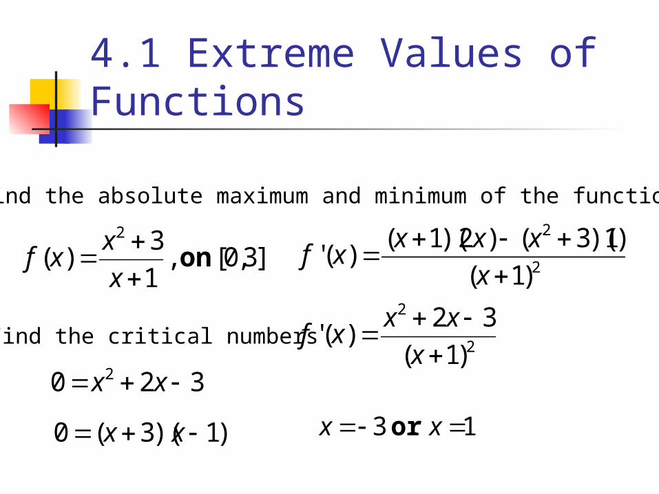
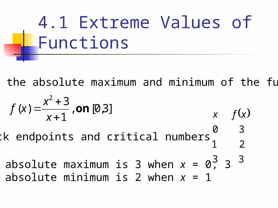
Find the absolute maximum and minimum of the function
]3,0[,1
3)(
2
on
x
xxf 2
2
)1(
)1)(3()2)(1()('
x
xxxxf
320 2 xx
Find the critical numbers
)1)(3(0 xx 13 xx or
2
2
)1(
32)('
x
xxxf
4.1 Extreme Values of Functions
Find the absolute maximum and minimum of the function
]3,0[,1
3)(
2
on
x
xxf
33
21
30
xfx
Check endpoints and critical numbers
The absolute maximum is 3 when x = 0, 3The absolute minimum is 2 when x = 1
4.1 Extreme Values of Functions
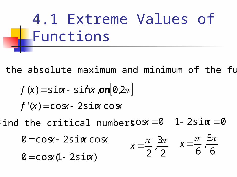
Find the absolute maximum and minimum of the function
2,0,sinsin)( 2 onxxxf
xxxxf cossin2cos)('
Find the critical numbers
xxx cossin2cos0
)sin21(cos0 xx
0cos x 0sin21 x
2
3,
2
x
6
5,
6
x
4.1 Extreme Values of Functions
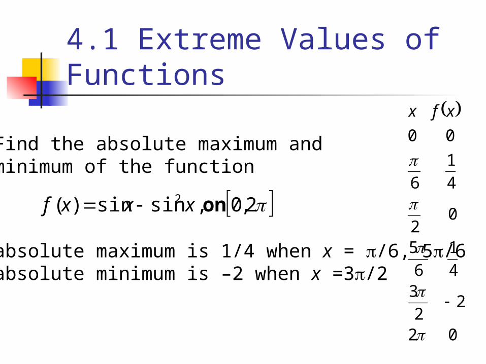
Find the absolute maximum andminimum of the function
2,0,sinsin)( 2 onxxxf
02
22
34
1
6
5
02
4
1
6
00
xfx
The absolute maximum is 1/4 when x = /6, 5/6The absolute minimum is –2 when x =3/2
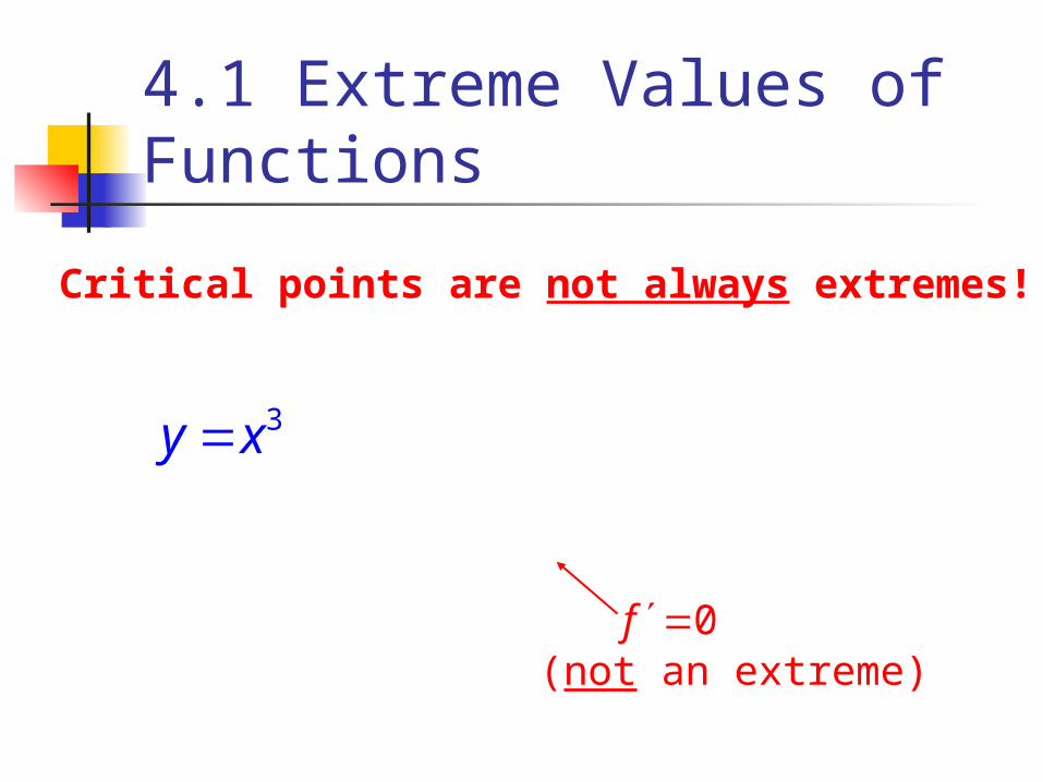
Critical points are not always extremes!
3y x
0f (not an extreme)
4.1 Extreme Values of Functions
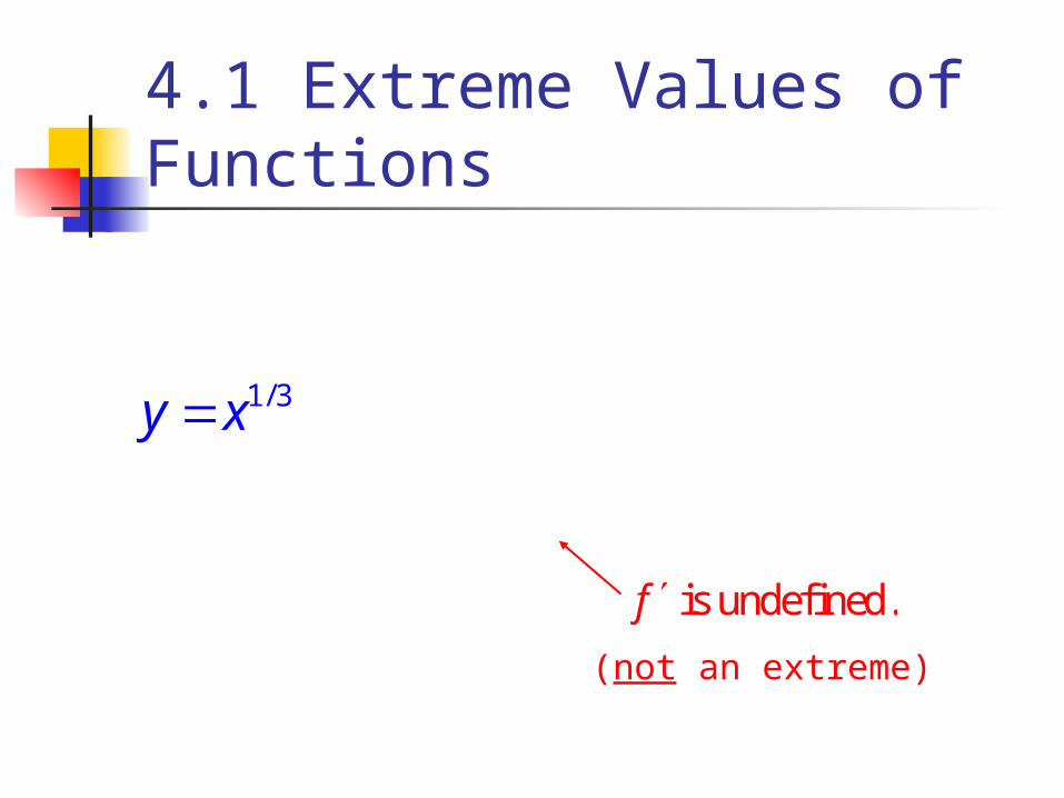
1/3y x
is undefined.f
(not an extreme)
4.1 Extreme Values of Functions

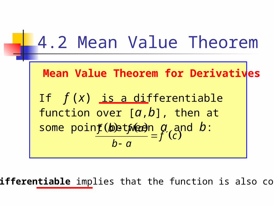
If f (x) is a differentiable function over [a,b], then at some point between a and b:
f b f af c
b a
Mean Value Theorem for Derivatives
4.2 Mean Value Theorem
If f (x) is a differentiable function over [a,b], then at some point between a and b:
f b f af c
b a
Mean Value Theorem for Derivatives
Differentiable implies that the function is also continuous.
4.2 Mean Value Theorem
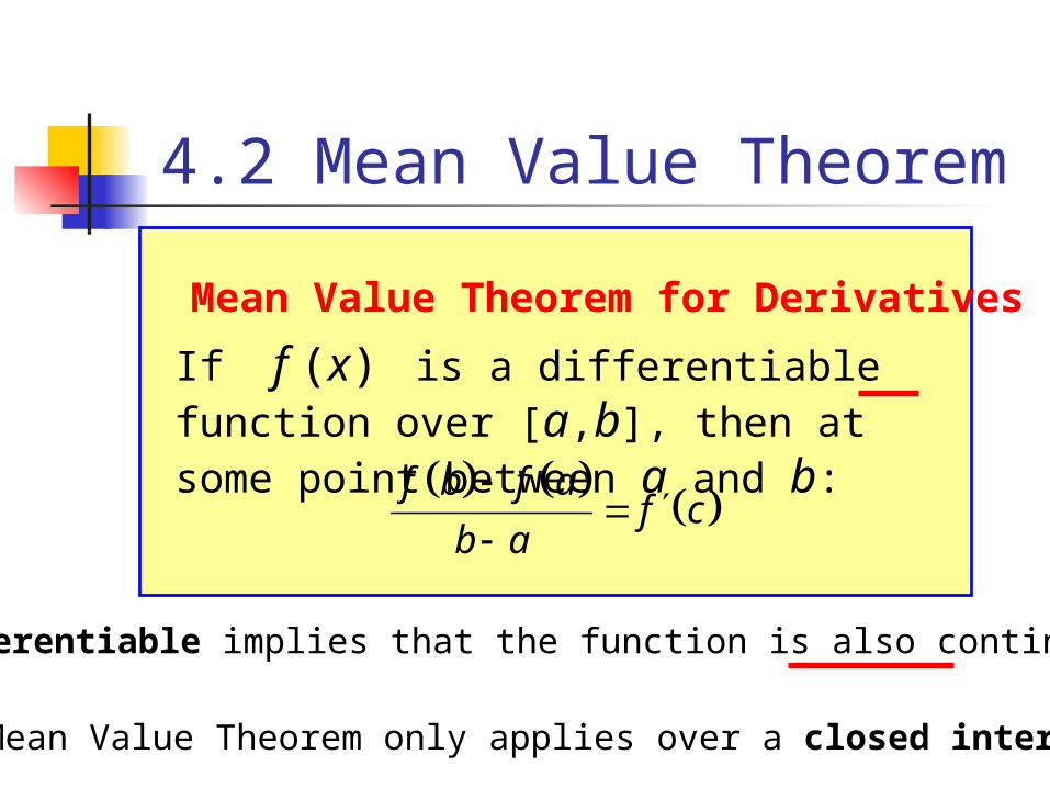
If f (x) is a differentiable function over [a,b], then at some point between a and b:
f b f af c
b a
Mean Value Theorem for Derivatives
Differentiable implies that the function is also continuous.
The Mean Value Theorem only applies over a closed interval.
4.2 Mean Value Theorem
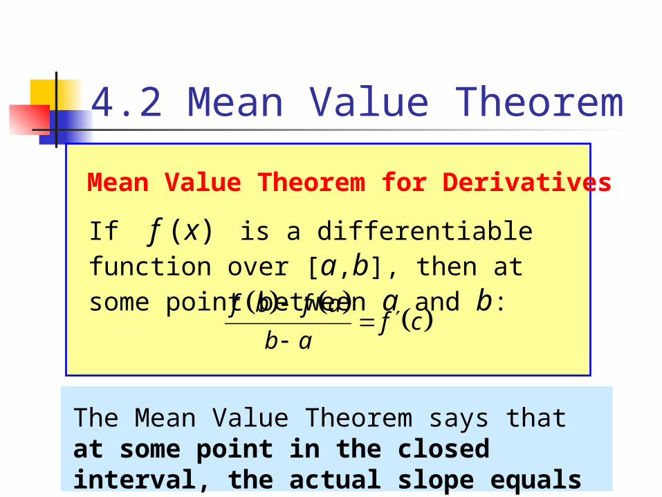
If f (x) is a differentiable function over [a,b], then at some point between a and b:
f b f af c
b a
Mean Value Theorem for Derivatives
The Mean Value Theorem says that at some point in the closed interval, the actual slope equals the average slope.
4.2 Mean Value Theorem

y
x0
A
B
a b
Slope of chord:
f b f a
b a
Slope of tangent:
f c
y f x
Tangent parallel to chord.
c
4.2 Mean Value Theorem
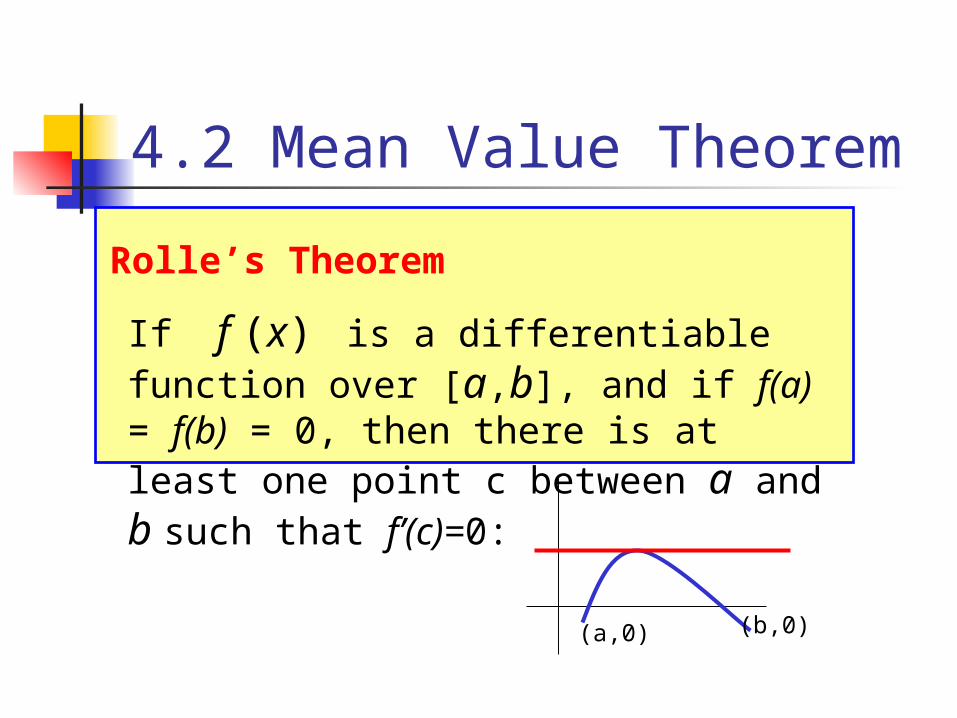
If f (x) is a differentiable function over [a,b], and if f(a) = f(b) = 0, then there is at least one point c between a and b such that f’(c)=0:
Rolle’s Theorem
4.2 Mean Value Theorem
(a,0) (b,0)
4.2 Mean Value Theorem
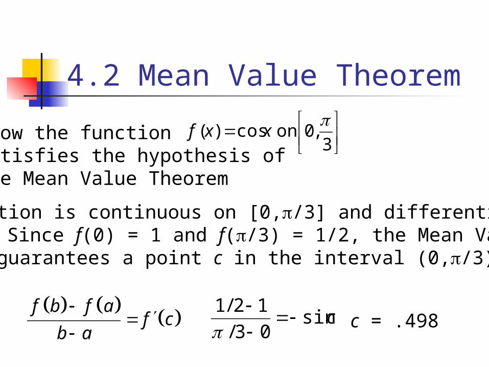
Show the function satisfies the hypothesis ofthe Mean Value Theorem
3,0oncos)(
xxf
The function is continuous on [0,/3] and differentiable on(0,/3). Since f(0) = 1 and f(/3) = 1/2, the Mean Value Theorem guarantees a point c in the interval (0,/3) for which
f b f af c
b a
csin
03/
12/1
c = .498
4.2 Mean Value Theorem
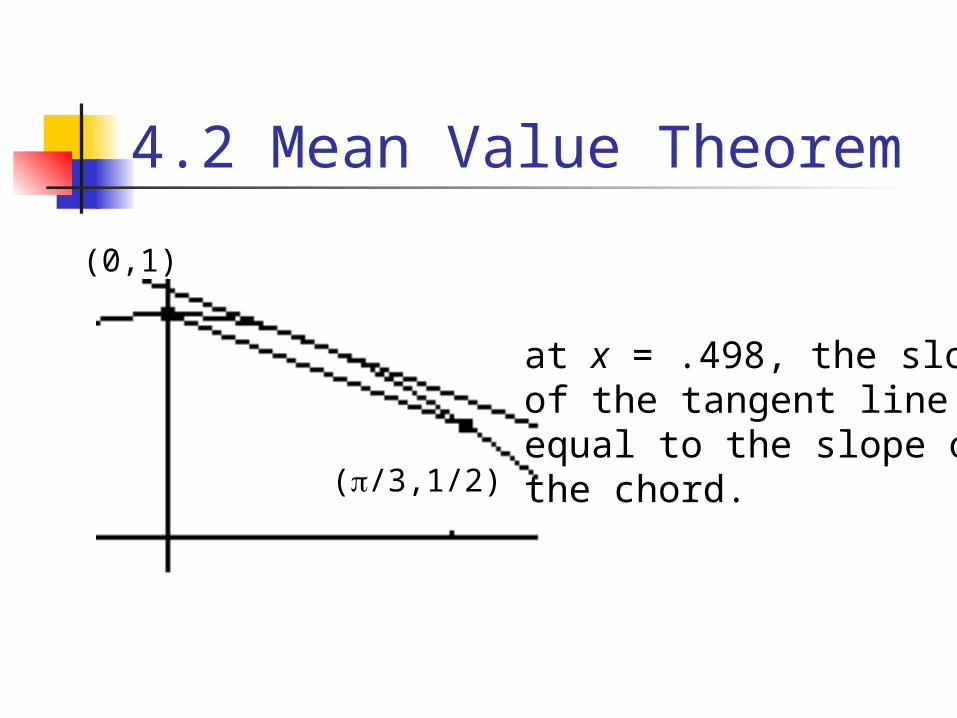
(0,1)
(/3,1/2)
at x = .498, the slopeof the tangent line isequal to the slope of the chord.
4.2 Mean Value Theorem
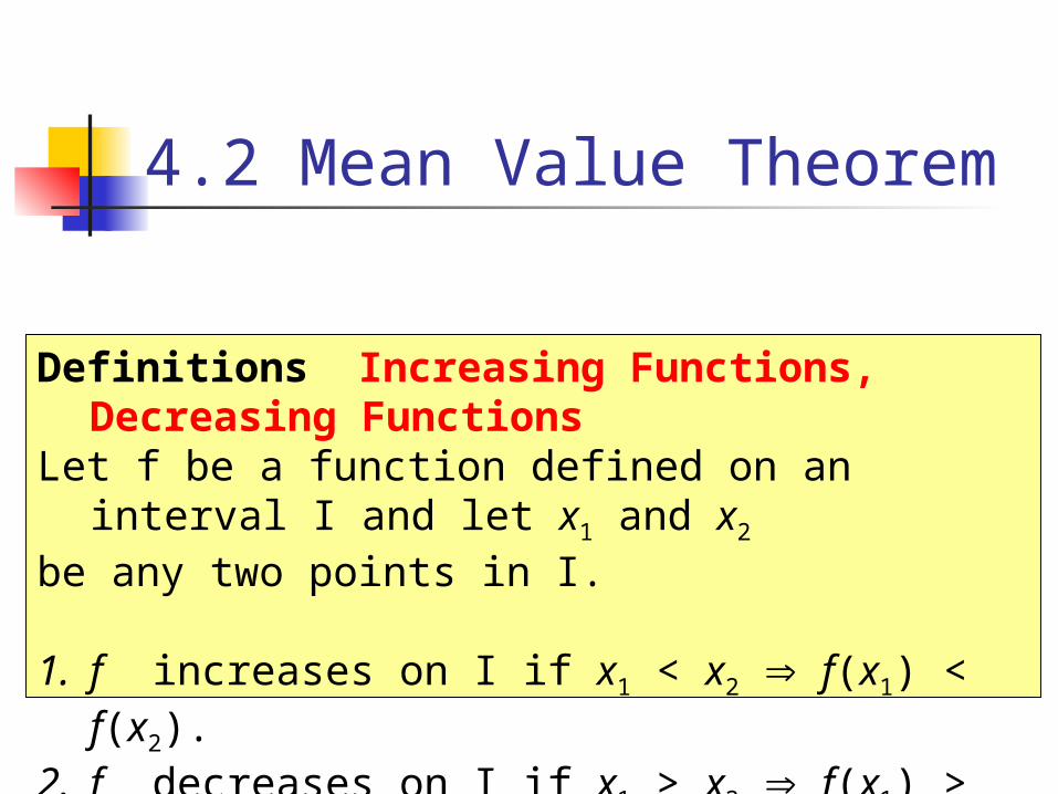
Definitions Increasing Functions, Decreasing FunctionsLet f be a function defined on an interval I and let x1 and x2
be any two points in I.
1. f increases on I if x1 < x2 f(x1) < f(x2).2. f decreases on I if x1 > x2 f(x1) > f(x2).
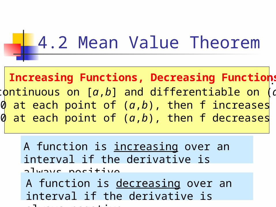
A function is increasing over an interval if the derivative is always positive.
A function is decreasing over an interval if the derivative is always negative.
A couple of somewhat obvious definitions:
4.2 Mean Value Theorem
Corollary Increasing Functions, Decreasing FunctionsLet f be continuous on [a,b] and differentiable on (a,b).1. If f’ > 0 at each point of (a,b), then f increases on [a,b].2. If f’ < 0 at each point of (a,b), then f decreases on [a,b].
4.2 Mean Value Theorem
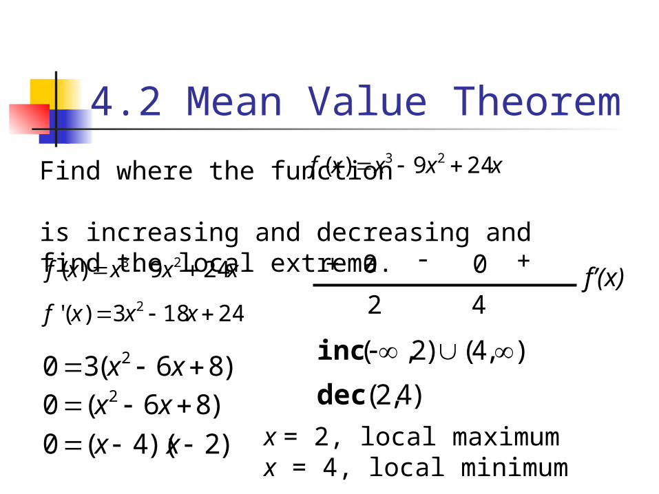
Find where the function is increasing and decreasing and find the local extrema.
xxxxf 249)( 23
xxxxf 249)( 23
24183)(' 2 xxxf
)86(30 2 xx
)86(0 2 xx
)2)(4(0 xx
2 4
0 0 f’(x)+-+
),4()2,( inc
)4,2(dec
x = 2, local maximum x = 4, local minimum

4.2 Mean Value Theorem
(2,20) local max
(4,16) local min
y
x0
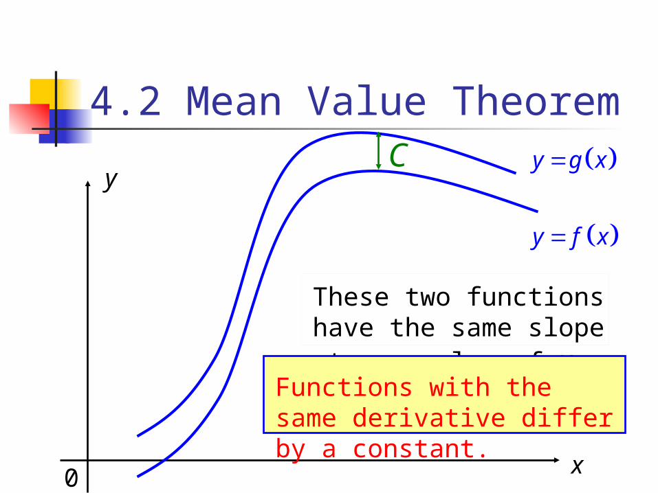
y f x
y g x
These two functions have the same slope at any value of x.
Functions with the same derivative differ by a constant.
C
4.2 Mean Value Theorem
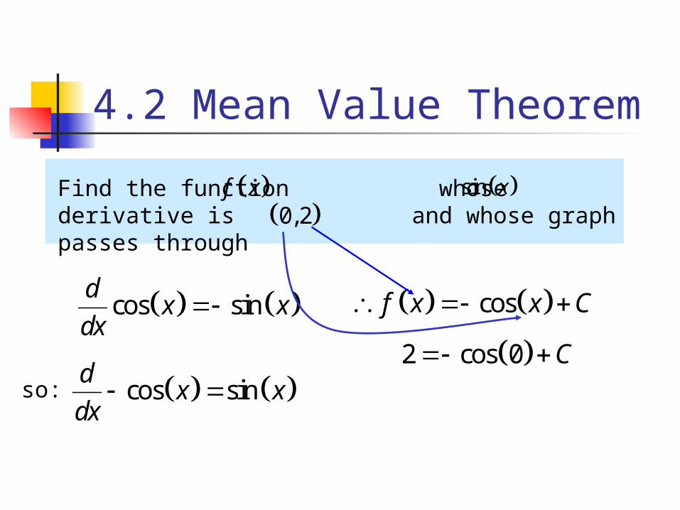
Find the function whose derivative is and whose graph passes through
f x sin x
0,2
cos sind
x xdx
cos sind
x xdx
so:
cosf x x C
2 cos 0 C
4.2 Mean Value Theorem

Find the function f(x) whose derivative is sin(x) and whose graph passes through (0,2).
cos sind
x xdx
cos sind
x xdx
so:
cosf x x C
2 cos 0 C 2 1 C
3 C
cos 3f x x Notice that we had to have initial values to determine the value of C.
4.2 Mean Value Theorem
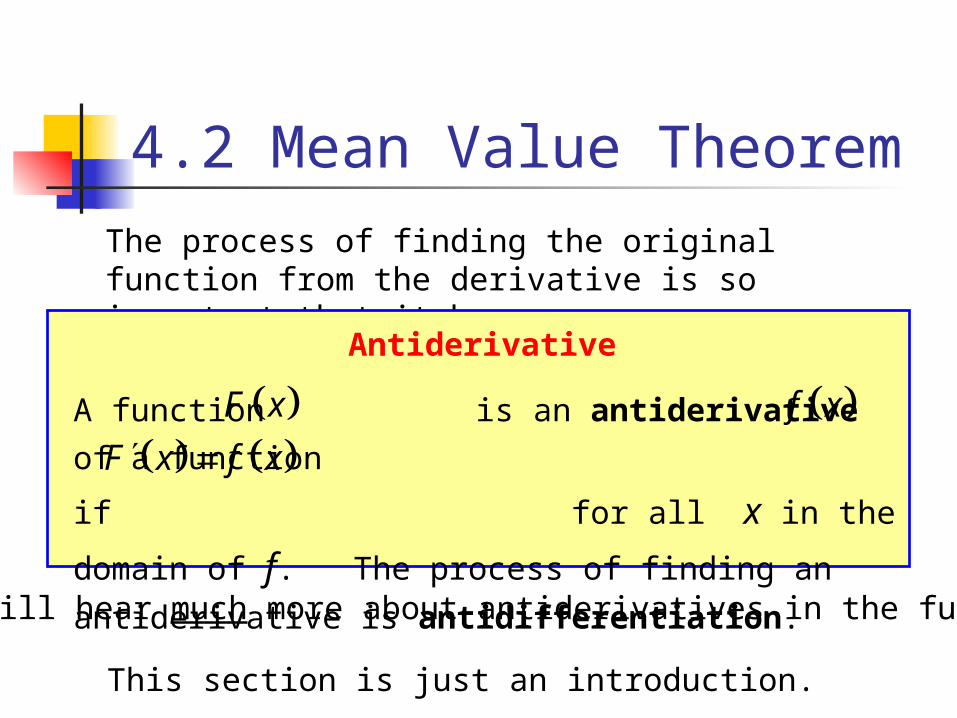
The process of finding the original function from the derivative is so important that it has a name:
Antiderivative
A function is an antiderivative of a function
if for all x in the domain of f. The process
of finding an antiderivative is antidifferentiation.
F x f x
F x f x
You will hear much more about antiderivatives in the future.
This section is just an introduction.
4.2 Mean Value Theorem

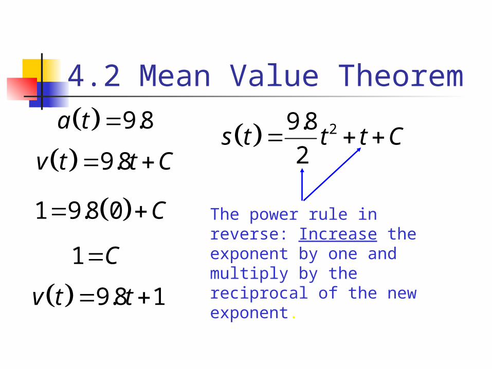
Since acceleration is the derivative of velocity, velocity must be the antiderivative of acceleration.
Example 7b: Find the velocity and position equations for a downward acceleration of 9.8 m/sec2 and an initial velocity of 1 m/sec downward.
9.8a t
9.8 1v t t
1 9.8 0 C
1 C
9.8v t t C (We let down be positive.)
4.2 Mean Value Theorem
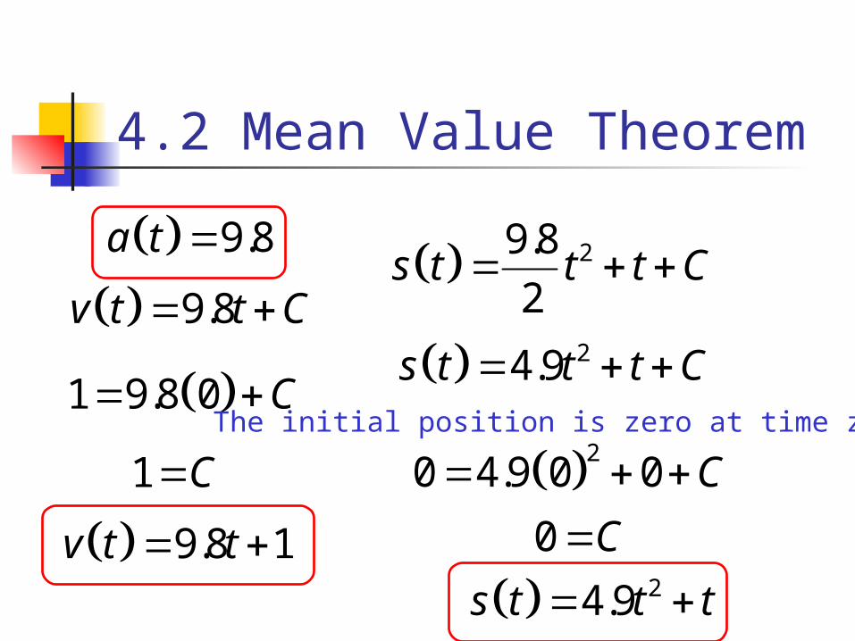
Since velocity is the derivative of position, position must be the antiderivative of velocity.
9.8a t
9.8 1v t t
1 9.8 0 C
1 C
9.8v t t C 29.8
2s t t t C
The power rule in reverse: Increase the exponent by one and multiply by the reciprocal of the new exponent.
4.2 Mean Value Theorem
9.8a t
9.8 1v t t
1 9.8 0 C
1 C
9.8v t t C 29.8
2s t t t C
24.9s t t t C The initial position is zero at time zero.
20 4.9 0 0 C
0 C
24.9s t t t
4.2 Mean Value Theorem

In the past, one of the important uses of derivatives was as an aid in curve sketching. We usually use a calculator of computer to draw complicated graphs, it is still important to understand the relationships between derivatives and graphs.
4.3 Connecting f’ and f’’ with the Graph of f

First Derivative Test for Local Extrema at a critical point c
4.3 Connecting f’ and f’’ with the Graph of f
1. If f ‘ changes sign from positive to negative at c, then f has a local maximum at c.
local max
f’>0 f’<0
2. If f ‘ changes sign from negative to positive at c, then f has a local minimum at c.
3. If f ‘ changes does not change sign at c, then f has no local extrema.
local min
f’<0 f’>0
no extreme
f’>0 f’>0
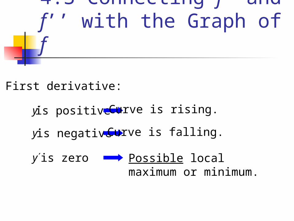
First derivative:
y is positive Curve is rising.
y is negative Curve is falling.
y is zero Possible local maximum or minimum.
4.3 Connecting f’ and f’’ with the Graph of f
4.3 Connecting f’ and f’’ with the Graph of f
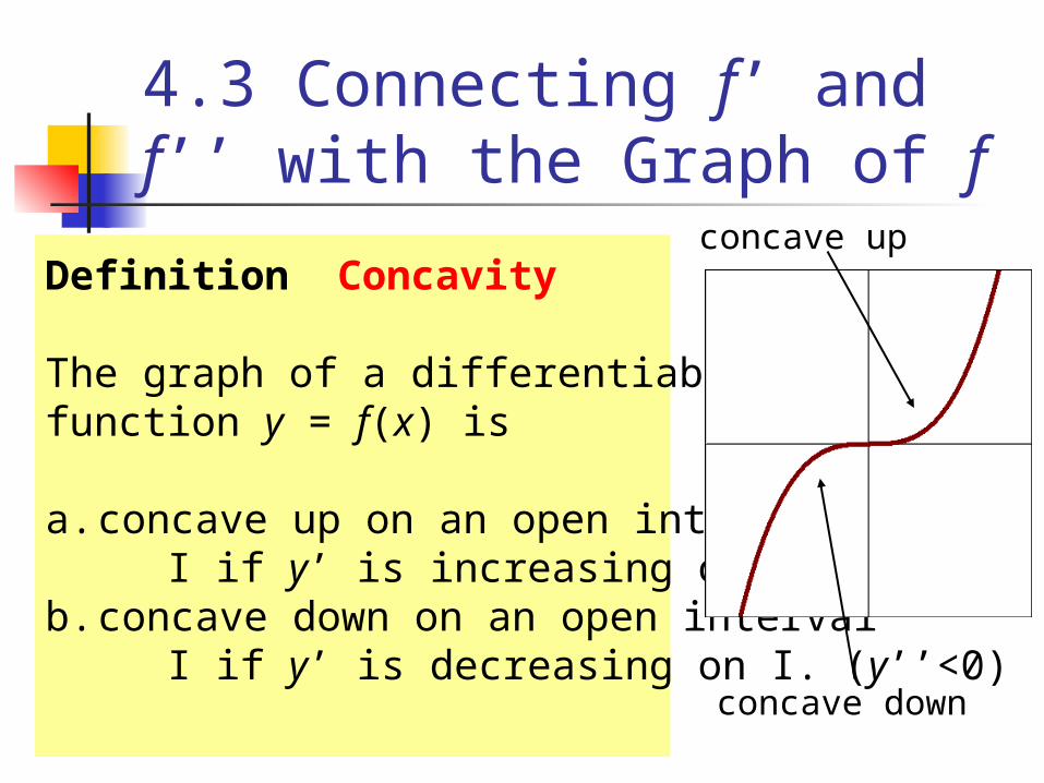
Definition Concavity
The graph of a differentiable function y = f(x) is
a. concave up on an open interval I if y’ is increasing on I. (y’’>0)b. concave down on an open interval I if y’ is decreasing on I. (y’’<0)
concave down
concave up

4.3 Connecting f’ and f’’ with the Graph of f
Second Derivative Test for Local Extrema at a critical point c
1. If f’(c) = 0 and f’’(c) < 0, then f has a local maximum at x = c.2. If f’(c) = 0 and f’’(c) > 0, then f has a local minimum at x = c.
+ +
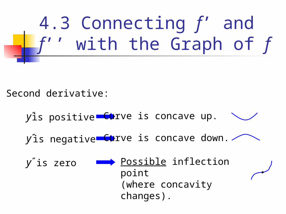
Second derivative:
y is positive Curve is concave up.
y is negative Curve is concave down.
y is zero Possible inflection point(where concavity changes).
4.3 Connecting f’ and f’’ with the Graph of f
4.3 Connecting f’ and f’’ with the Graph of f
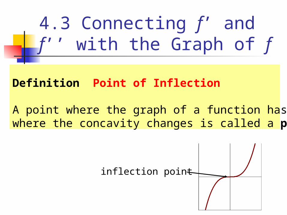
Definition Point of Inflection
A point where the graph of a function has a tangent line andwhere the concavity changes is called a point of inflection.
inflection point

23 23 4 1 2y x x x x
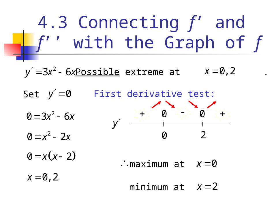
23 6y x x 0ySet
20 3 6x x 20 2x x
0 2x x 0, 2x
First derivative test:
y0 2
0 0
21 3 1 6 1 3y negative
21 3 1 6 1 9y positive
23 3 3 6 3 9y positive
Possible extreme at .0, 2x
4.3 Connecting f’ and f’’ with the Graph of f
Sketch the graph
zeros at x = -1, x = 2
23 6y x x
0ySet
20 3 6x x
20 2x x
0 2x x
0, 2x
First derivative test:
y0 2
0 0
maximum at 0x
minimum at 2x
Possible extreme at .0, 2x
4.3 Connecting f’ and f’’ with the Graph of f
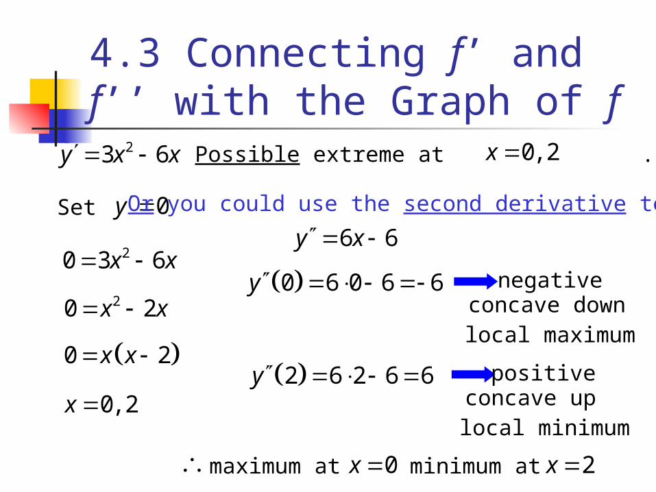
23 6y x x
0ySet
20 3 6x x
20 2x x
0 2x x
0, 2x
Possible extreme at .0, 2x
Or you could use the second derivative test:
maximum at 0x minimum at 2x
6 6y x
0 6 0 6 6y negativeconcave downlocal maximum
2 6 2 6 6y positiveconcave uplocal minimum
4.3 Connecting f’ and f’’ with the Graph of f
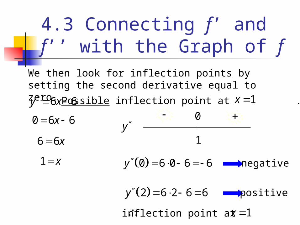
6 6y x
We then look for inflection points by setting the second derivative equal to zero.
0 6 6x
6 6x
1 x
Possible inflection point at .1x
y1
0
0 6 0 6 6y negative
2 6 2 6 6y positive
inflection point at 1x
4.3 Connecting f’ and f’’ with the Graph of f
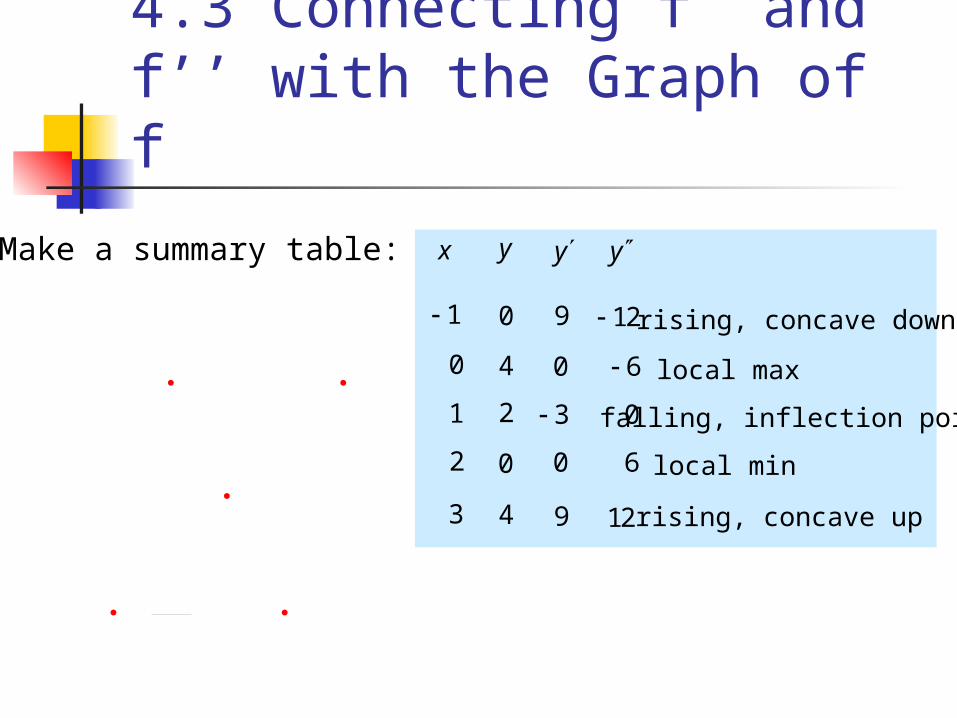
Make a summary table: x y y y
1 0 9 12 rising, concave down
0 4 0 6 local max
1 2 3 0 falling, inflection point
2 0 0 6 local min
3 4 9 12 rising, concave up
4.3 Connecting f’ and f’’ with the Graph of f
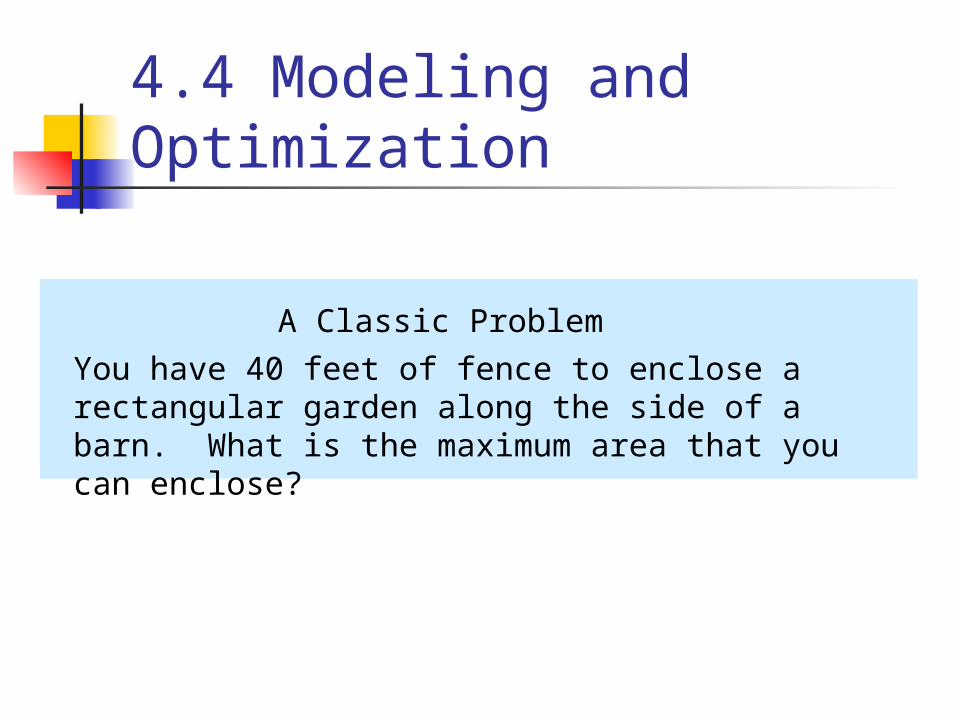
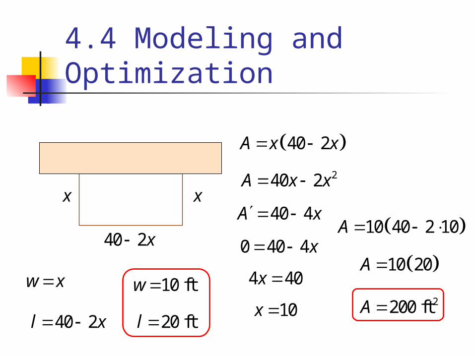
A Classic Problem
You have 40 feet of fence to enclose a rectangular garden along the side of a barn. What is the maximum area that you can enclose?
4.4 Modeling and Optimization
x x
40 2x
40 2A x x
240 2A x x
40 4A x
0 40 4x
4 40x
10x
10 40 2 10A
10 20A
2200 ftA 40 2l x
w x 10 ftw
20 ftl
4.4 Modeling and Optimization
To find the maximum (or minimum) value of a function:
4.4 Modeling and Optimization
1. Understand the Problem.2. Develop a Mathematical Model.3. Graph the Function.4. Identify Critical Points and Endpoints.5. Solve the Mathematical Model.6. Interpret the Solution.

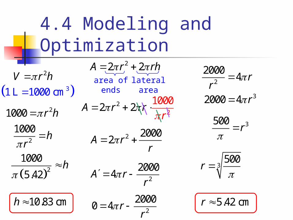
What dimensions for a one liter cylindrical can will use the least amount of material?
We can minimize the material by minimizing the area.
22 2A r rh
area ofends
lateralarea
We need another equation that relates r and h:
2V r h
31 L 1000 cm
21000 r h
2
1000h
r
22
10 02
02A r r
r
2 20002A r
r
2
20004A r
r
4.4 Modeling and Optimization
22 2A r rh area ofends
lateralarea
2V r h
31 L 1000 cm21000 r h
2
1000h
r
22
10 02
02A r r
r
2 20002A r
r
2
20004A r
r
2
20000 4 r
r
2
20004 r
r
32000 4 r
3500r
3500
r
5.42 cmr
2
1000
5.42h
10.83 cmh
4.4 Modeling and Optimization
4.4 Modeling and Optimization
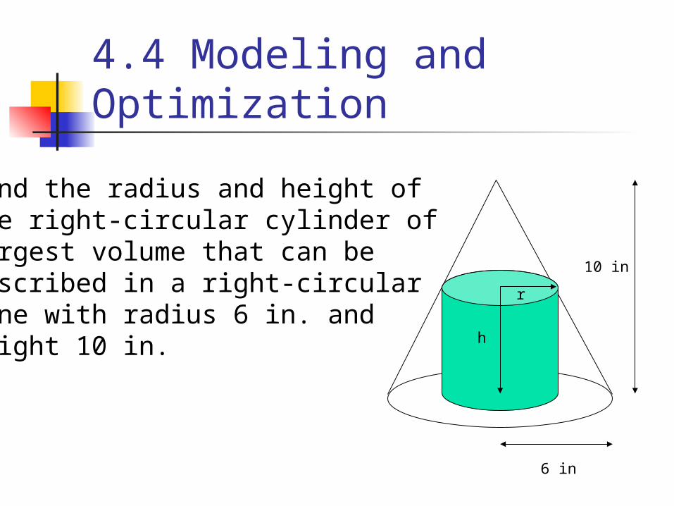
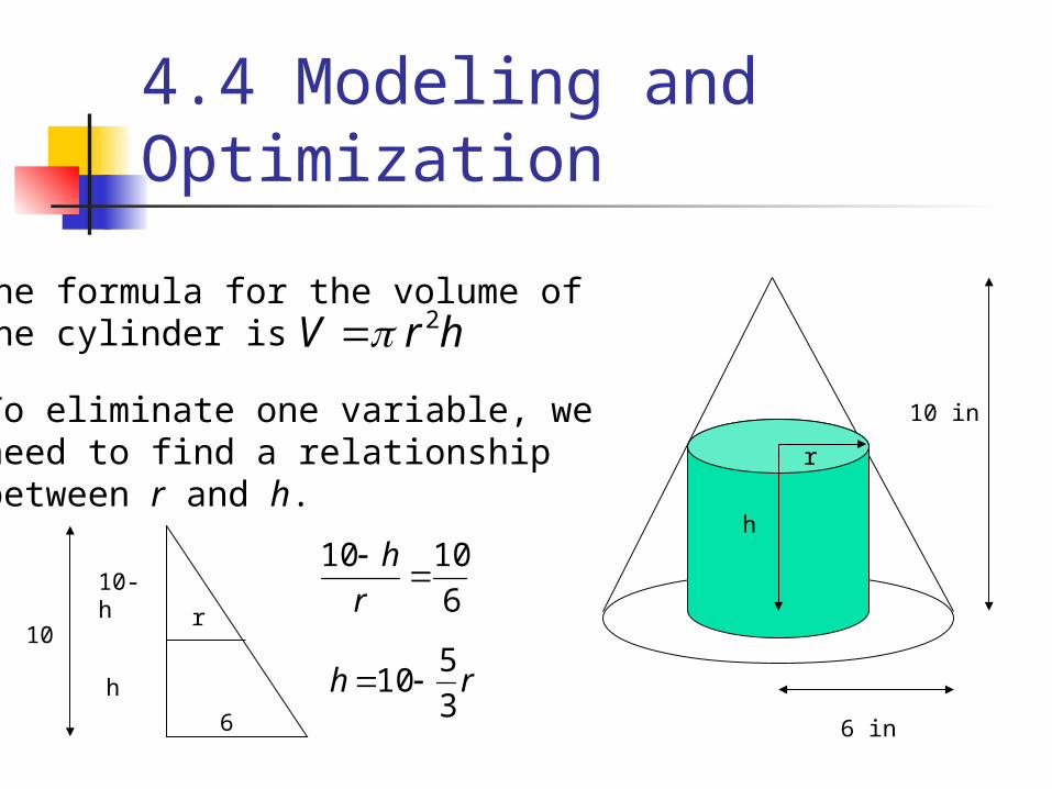
Find the radius and height ofthe right-circular cylinder oflargest volume that can beinscribed in a right-circularcone with radius 6 in. andheight 10 in. h
r
10 in
6 in
4.4 Modeling and Optimization
h
r
10 in
6 in
The formula for the volume ofthe cylinder is hrV 2
To eliminate one variable, weneed to find a relationshipbetween r and h.
6
1010
r
h
rh3
510
6
h
10-h
r10
4.4 Modeling and Optimization
h
r
10 in
6 in
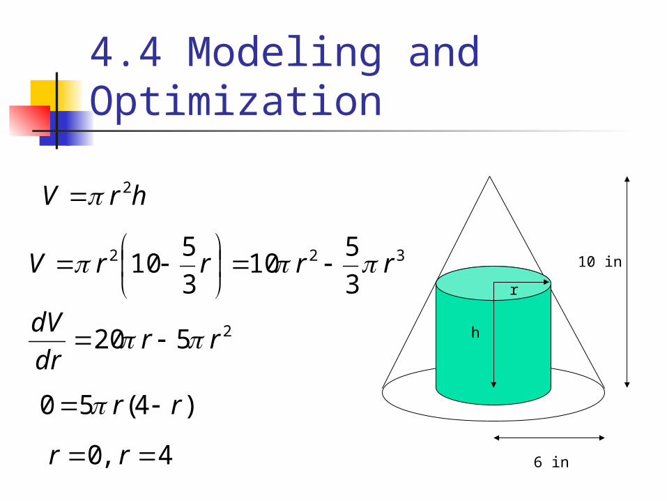
hrV 2
322
3
510
3
510 rrrrV
2520 rrdr
dV
)4(50 rr
4,0 rr
4.4 Modeling and Optimization
h
r
10 in
6 in
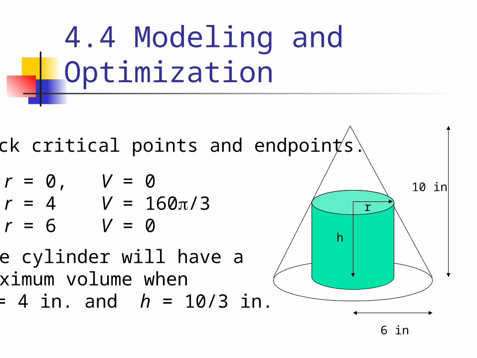
Check critical points and endpoints.
•r = 0, V = 0•r = 4 V = 160/3•r = 6 V = 0
The cylinder will have a maximum volume when r = 4 in. and h = 10/3 in.
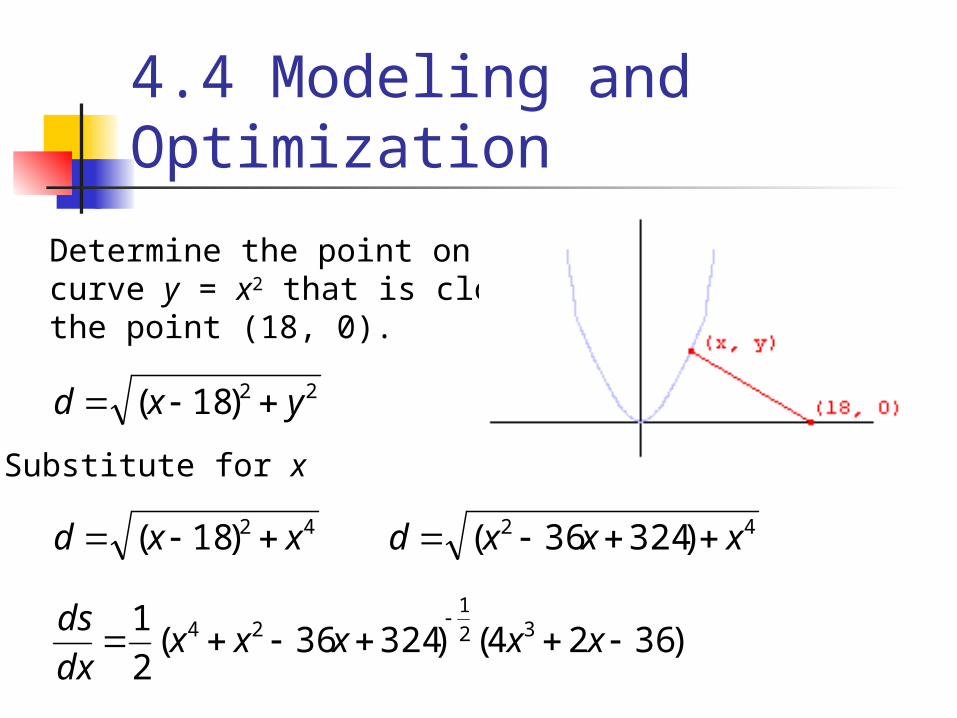
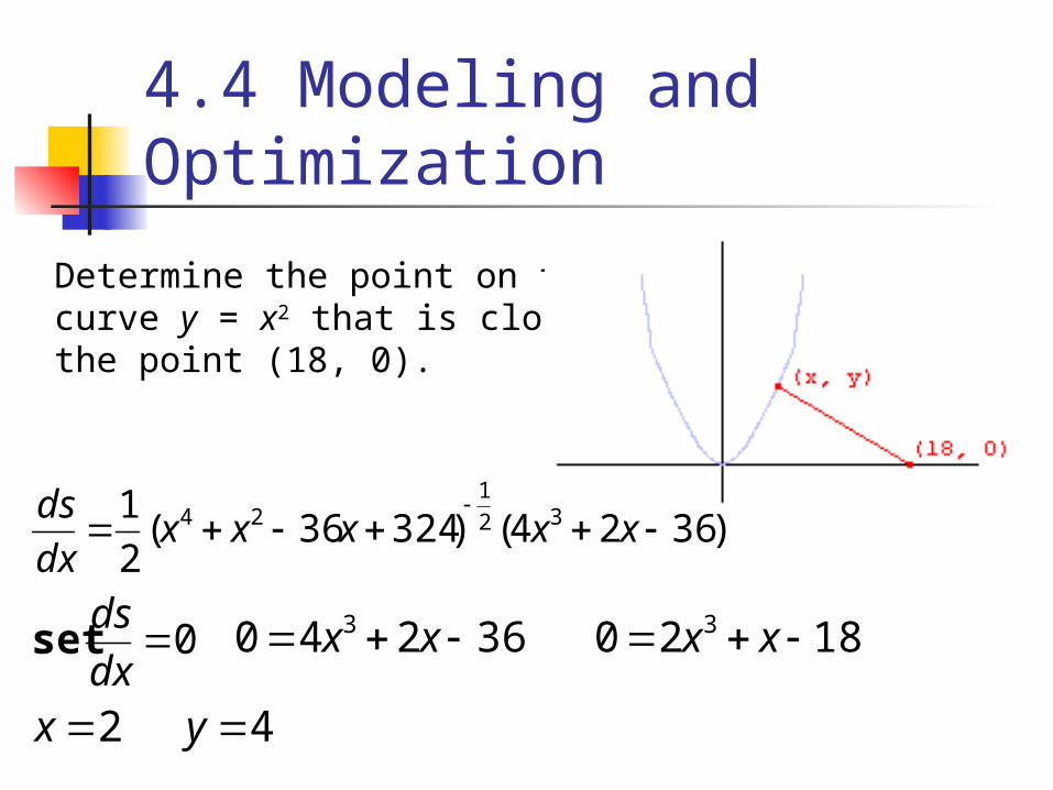
Determine the point on the curve y = x2 that is closest to the point (18, 0).
4.4 Modeling and Optimization
22)18( yxd
42)18( xxd
Substitute for x
42 )32436( xxxd
)3624()32436(2
1 32
124
xxxxx
dx
ds
Determine the point on the curve y = x2 that is closest to the point (18, 0).
4.4 Modeling and Optimization
)3624()32436(2
1 32
124
xxxxx
dx
ds
0dx
dsset 36240 3 xx 1820 3 xx
2x 4y
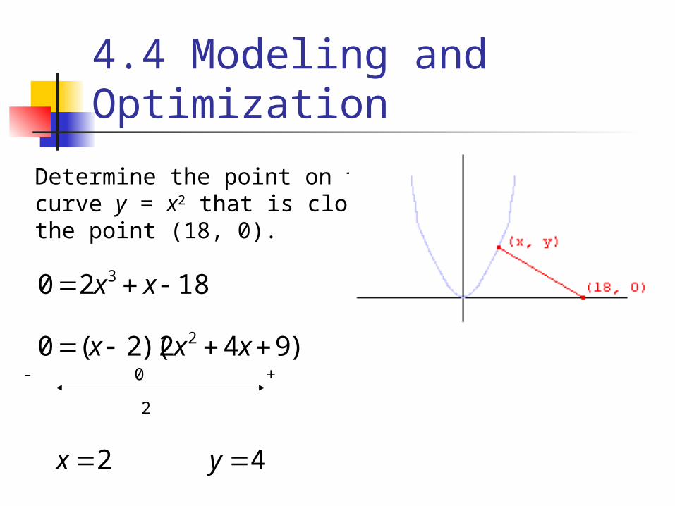
Determine the point on the curve y = x2 that is closest to the point (18, 0).
4.4 Modeling and Optimization
1820 3 xx
2x 4y
)942)(2(0 2 xxx
2
- 0 +
If the end points could be the maximum or minimum, you have to check.
Notes:
If the function that you want to optimize has more than one variable, use substitution to rewrite the function.
If you are not sure that the extreme you’ve found is a maximum or a minimum, you have to check.
4.4 Modeling and Optimization
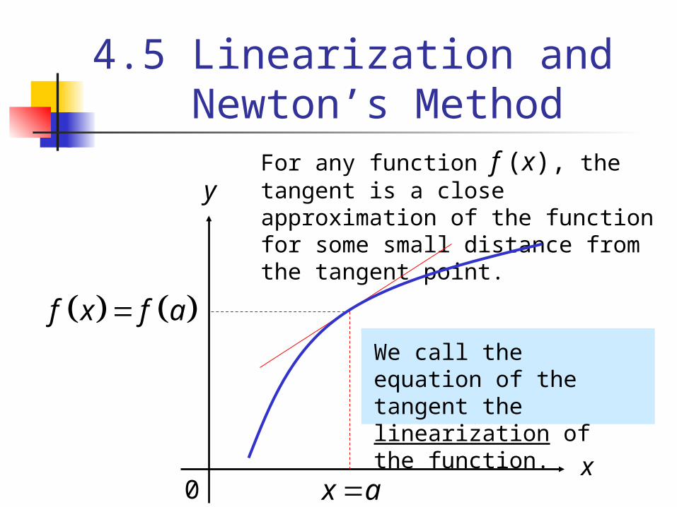
For any function f (x), the tangent is a close approximation of the function for some small distance from the tangent point.
y
x0 x a
f x f aWe call the equation of the tangent the linearization of the function.
4.5 Linearization and Newton’s Method
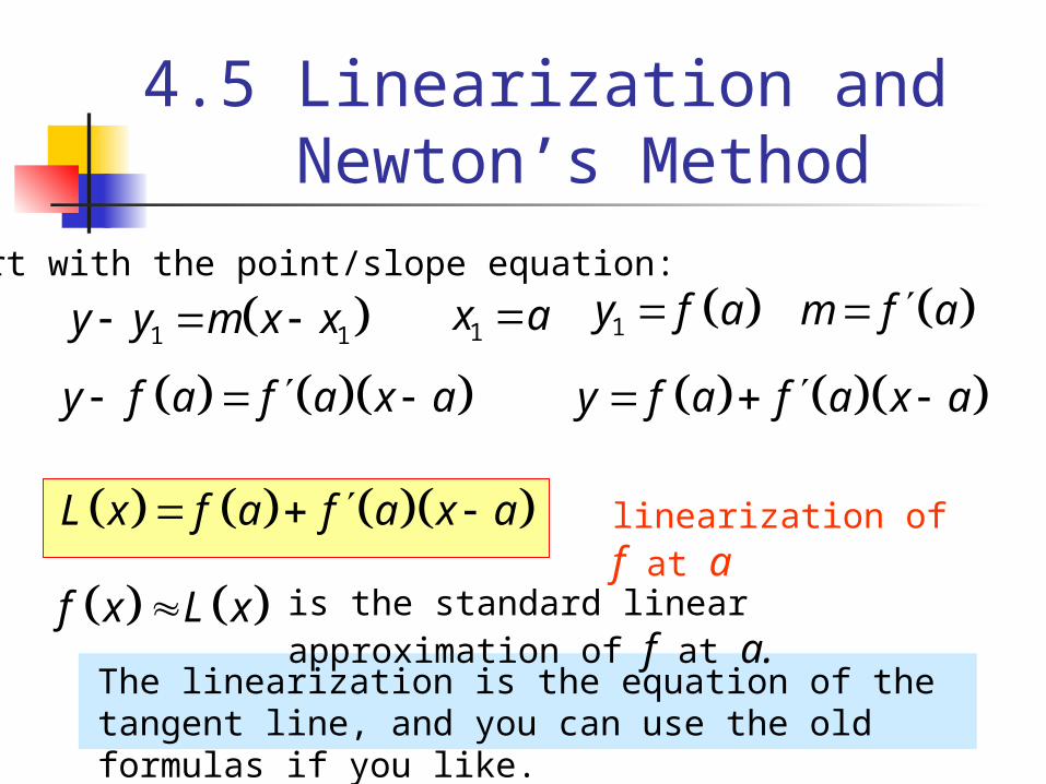
The linearization is the equation of the tangent line, and you can use the old formulas if you like.
Start with the point/slope equation:
1 1y y m x x 1x a 1y f a m f a
y f a f a x a y f a f a x a
L x f a f a x a linearization of f at a
f x L x is the standard linear approximation of f at a.
4.5 Linearization and Newton’s Method
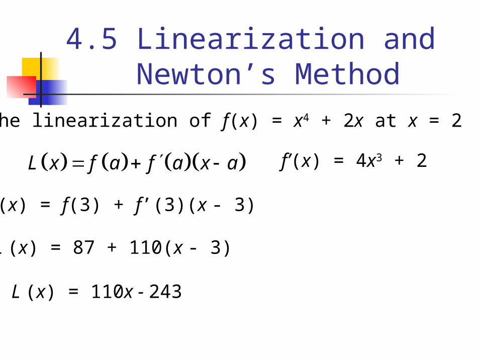
Find the linearization of f(x) = x4 + 2x at x = 2
L x f a f a x a
4.5 Linearization and Newton’s Method
f’(x) = 4x3 + 2
L (x) = f(3) + f’(3)(x - 3)
L (x) = 87 + 110(x - 3)
L (x) = 110x - 243
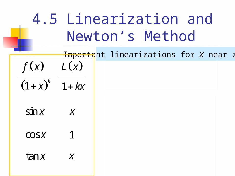
Important linearizations for x near zero:
1k
x 1 kx
sin x
cos x
tan x
x
1
x
1
21
1 1 12
x x x
13 4 4 3
4 4
1 5 1 5
1 51 5 1
3 3
x x
x x
f x L x
This formula also leads to non-linear approximations:
4.5 Linearization and Newton’s Method
4.5 Linearization and Newton’s Method
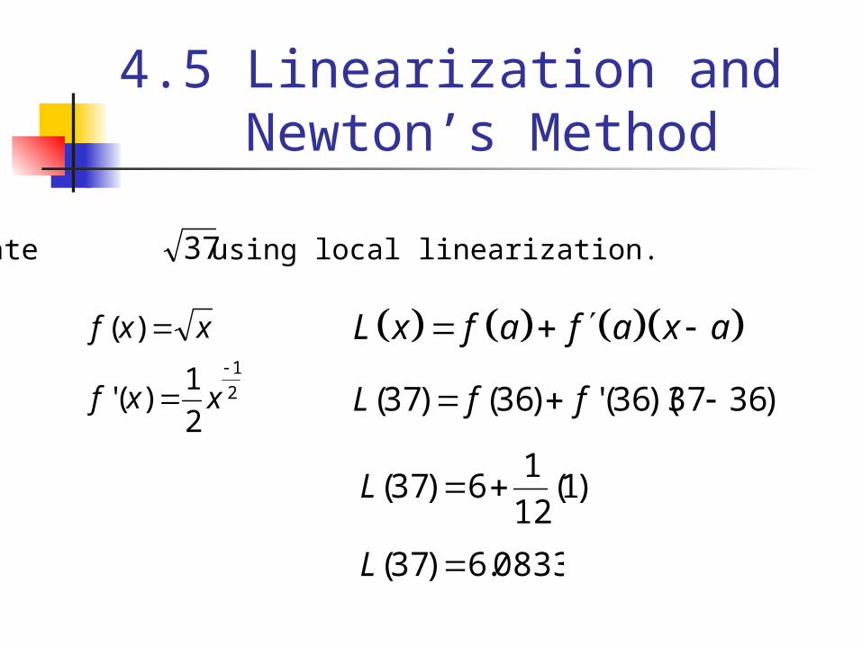
Estimate using local linearization. 37
2
1
2
1)('
)(
xxf
xxf L x f a f a x a
)3637)(36(')36()37( ffL
)1(12
16)37( L
0833.6)37( L
4.5 Linearization and Newton’s Method
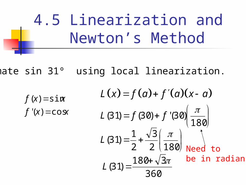
Estimate sin 31º using local linearization.
xxf
xxf
cos)('
sin)(
L x f a f a x a
180
)30(')30()31(
ffL
1802
3
2
1)31(
L
360
3180)31(
L
Need tobe in radians
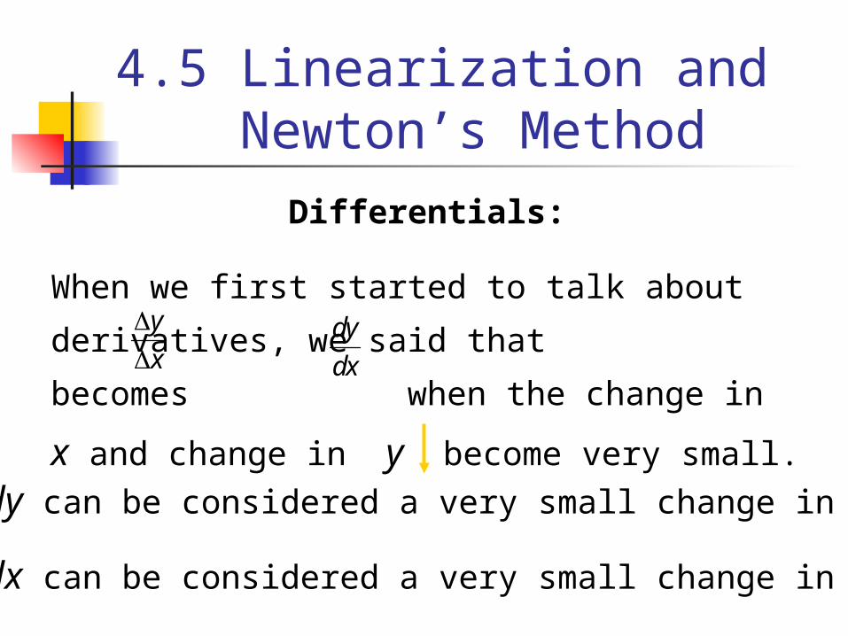
Differentials:
When we first started to talk about derivatives, we said
that becomes when the change in x and
change in y become very small.
y
x
dy
dx
dy can be considered a very small change in y.
dx can be considered a very small change in x.
4.5 Linearization and Newton’s Method
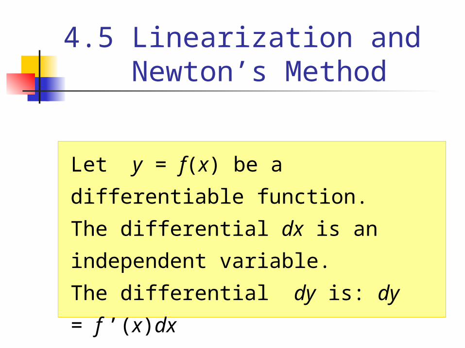
Let y = f(x) be a differentiable function.
The differential dx is an independent
variable.
The differential dy is: dy = f ’(x)dx
4.5 Linearization and Newton’s Method
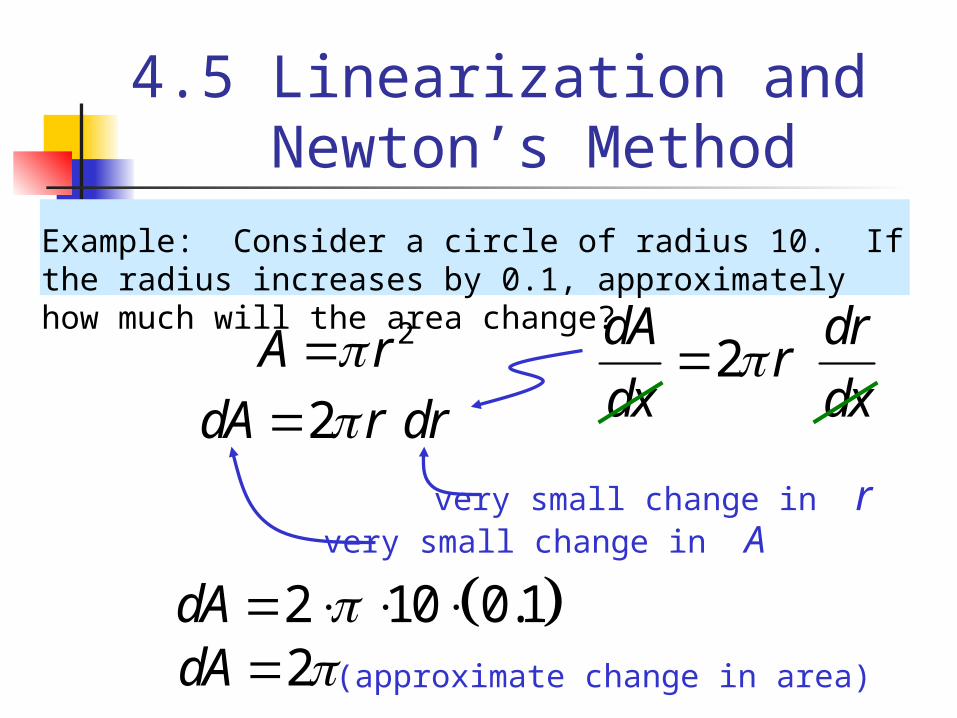
Example: Consider a circle of radius 10. If the radius increases by 0.1, approximately how much will the area change?
2A r2 dA r dr
2 dA dr
rdx dx
very small change in Avery small change in r
2 10 0.1dA 2dA (approximate change in area)
4.5 Linearization and Newton’s Method
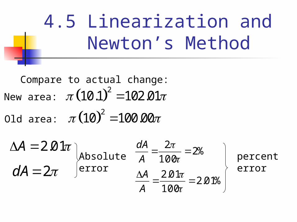
Compare to actual change:
New area:
Old area:
210.1 102.01
210 100.00
4.5 Linearization and Newton’s Method
01.2A
2dAAbsoluteerror
%2100
2
A
dA
%01.2100
01.2
A
A
percenterror
4.5 Linearization and Newton’s Method
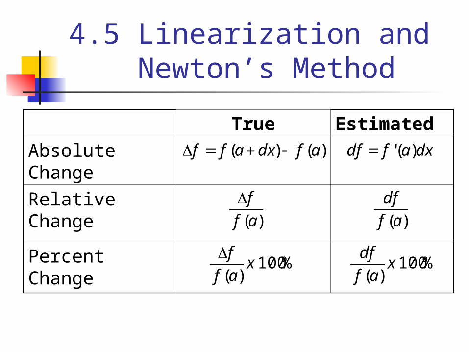
True Estimated
Absolute Change
Relative Change
Percent Change
)()( afdxaff dxafdf )('
)(af
f)(af
df
%100)(
xaf
df%100
)(x
af
f
4.5 Linearization and Newton’s Method
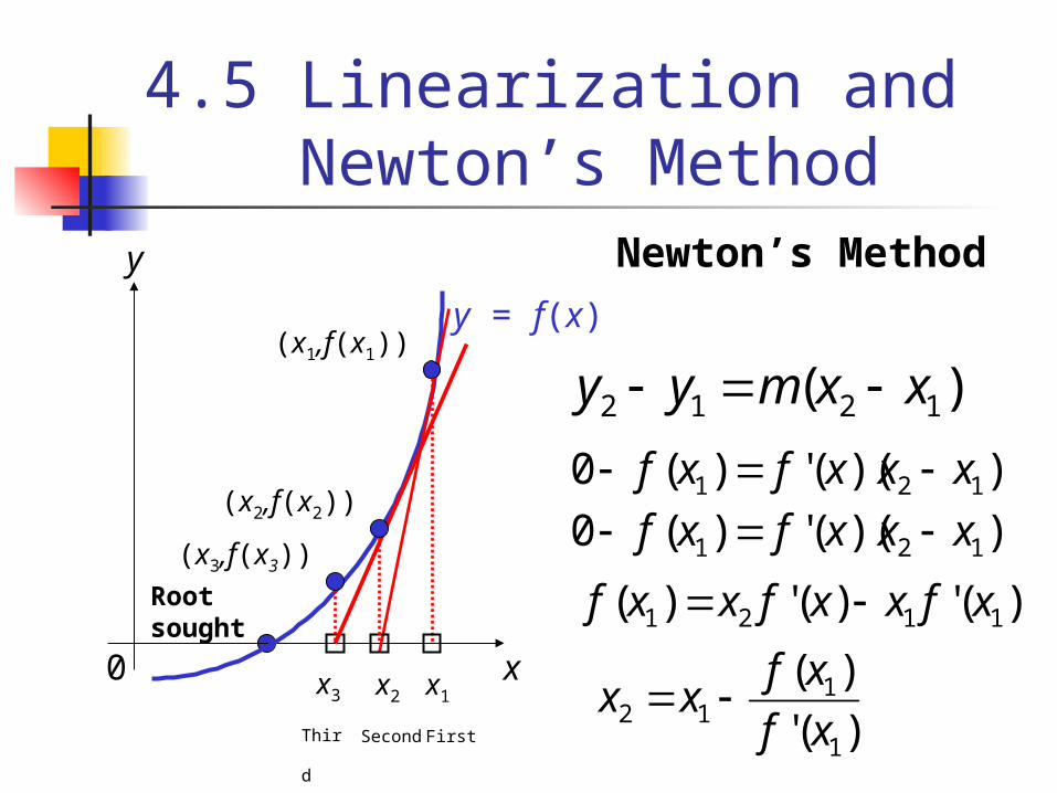
Newton’s Method
0 x
y
y = f(x)
Rootsought
x1
First
(x1,f(x1))
x2
Second
x3
Third
(x2,f(x2))
(x3,f(x3))
)( 1212 xxmyy
))((')(0 121 xxxfxf ))((')(0 121 xxxfxf
)(')(')( 1121 xfxxfxxf
)('
)(
1
112 xf
xfxx
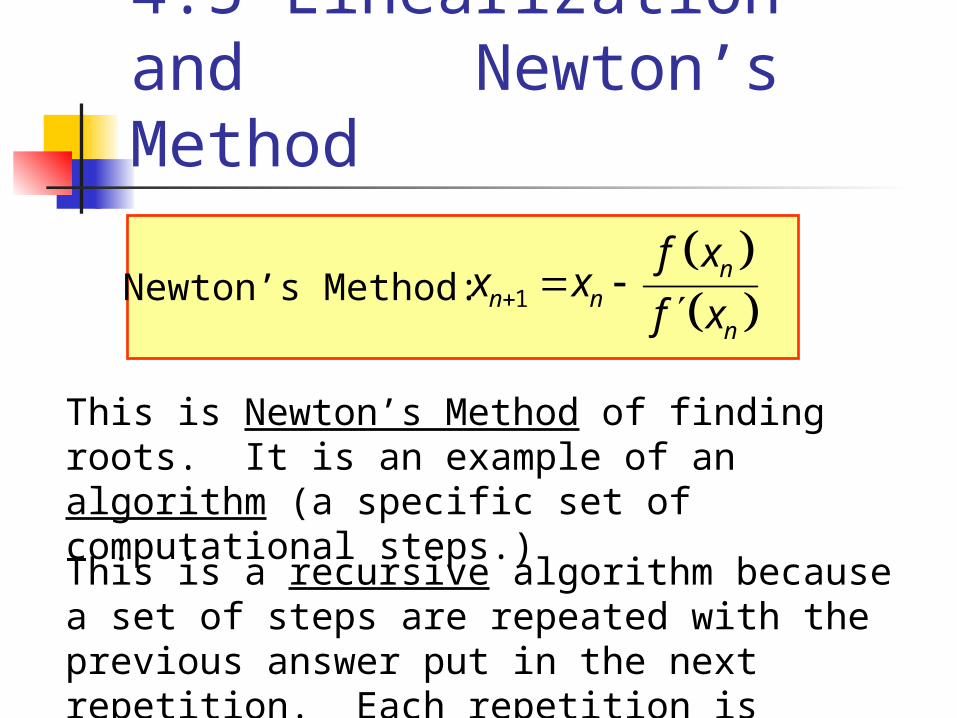
This is Newton’s Method of finding roots. It is an example of an algorithm (a specific set of computational steps.)
Newton’s Method: 1
nn n
n
f xx x
f x
This is a recursive algorithm because a set of steps are repeated with the previous answer put in the next repetition. Each repetition is called an iteration.
4.5 Linearization and Newton’s Method
Newton’s Method
213
2f x x
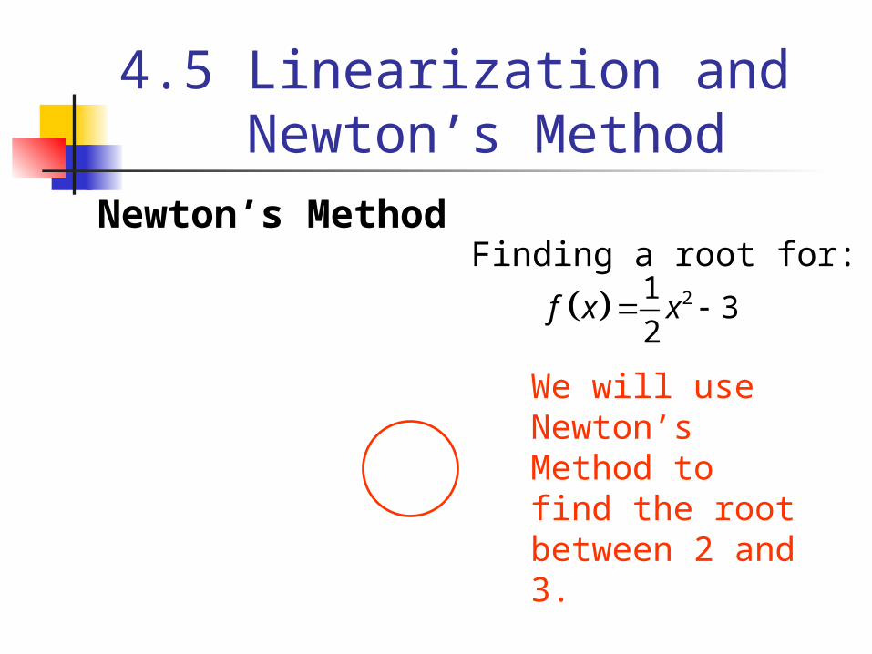
Finding a root for:
We will use Newton’s Method to find the root between 2 and 3.
4.5 Linearization and Newton’s Method
Newton’s Method 213
2f x x
4.5 Linearization and Newton’s Method
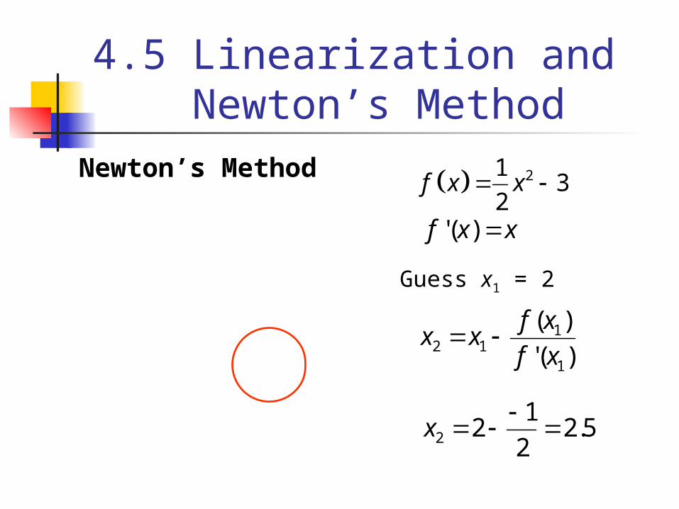
xxf )('
Guess x1 = 2
)('
)(
1
112 xf
xfxx
5.22
122
x
Newton’s Method 213
2f x x
4.5 Linearization and Newton’s Method
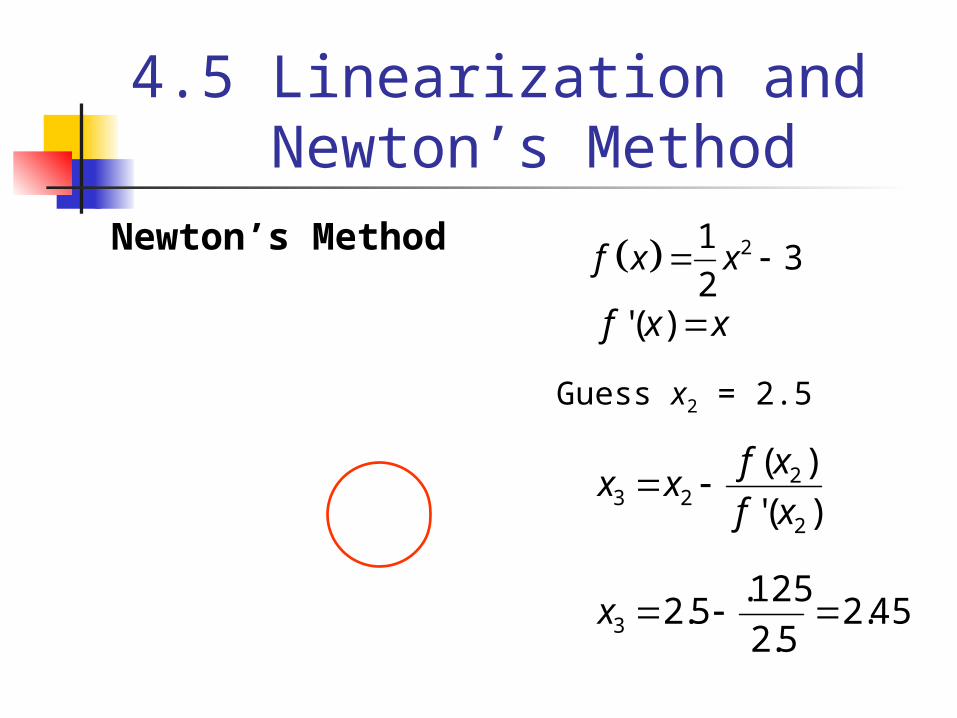
xxf )('
Guess x2 = 2.5
)('
)(
2
223 xf
xfxx
45.25.2
125.5.23 x
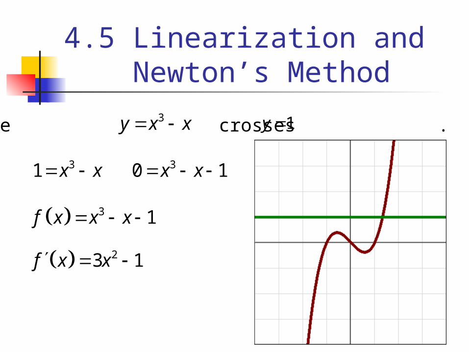
Find where crosses .3y x x 1y
31 x x 30 1x x
3 1f x x x
23 1f x x
4.5 Linearization and Newton’s Method
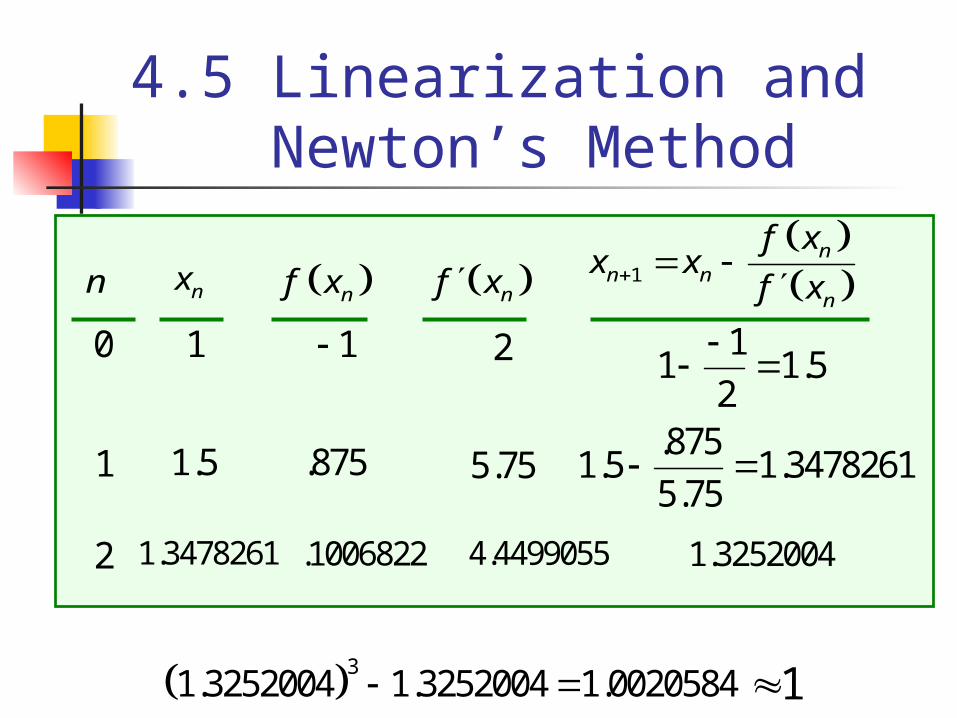
nx nf xn nf x 1
nn n
n
f xx x
f x
0 1 1 2 11 1.5
2
1 1.5 .875 5.75.875
1.5 1.34782615.75
2 1.3478261 .1006822 4.4499055 1.3252004
31.3252004 1.3252004 1.0020584 1
4.5 Linearization and Newton’s Method
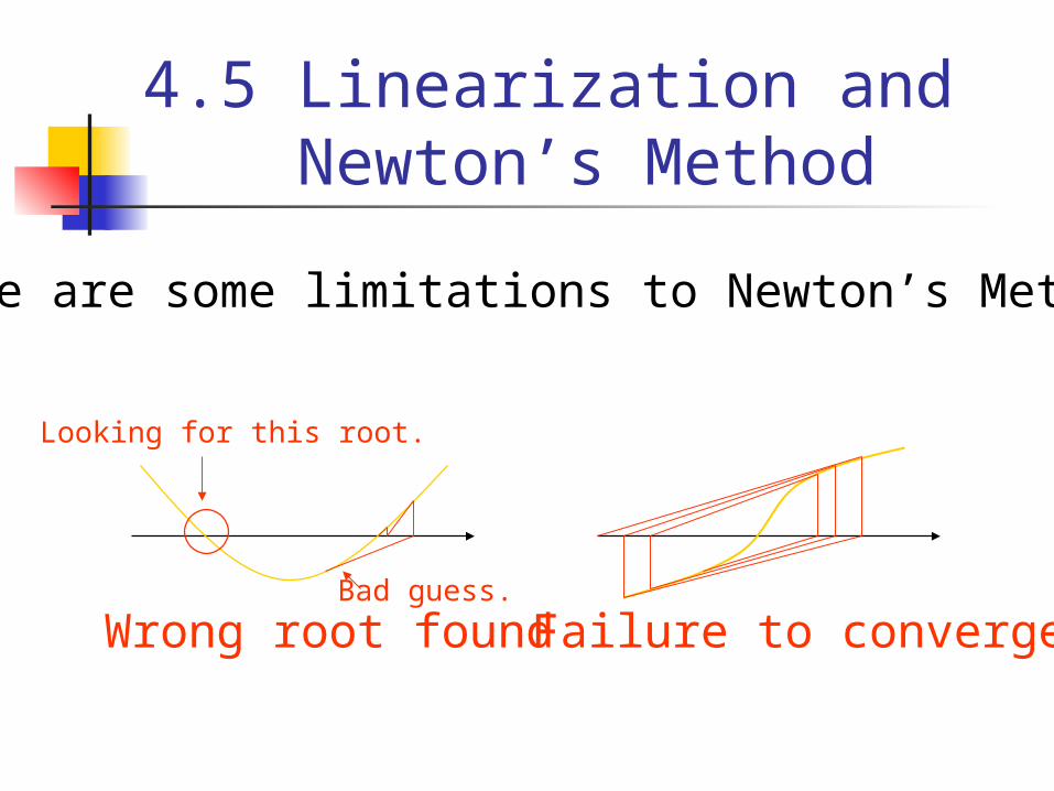
There are some limitations to Newton’s Method:
Wrong root found
Looking for this root.
Bad guess.
Failure to converge
4.5 Linearization and Newton’s Method
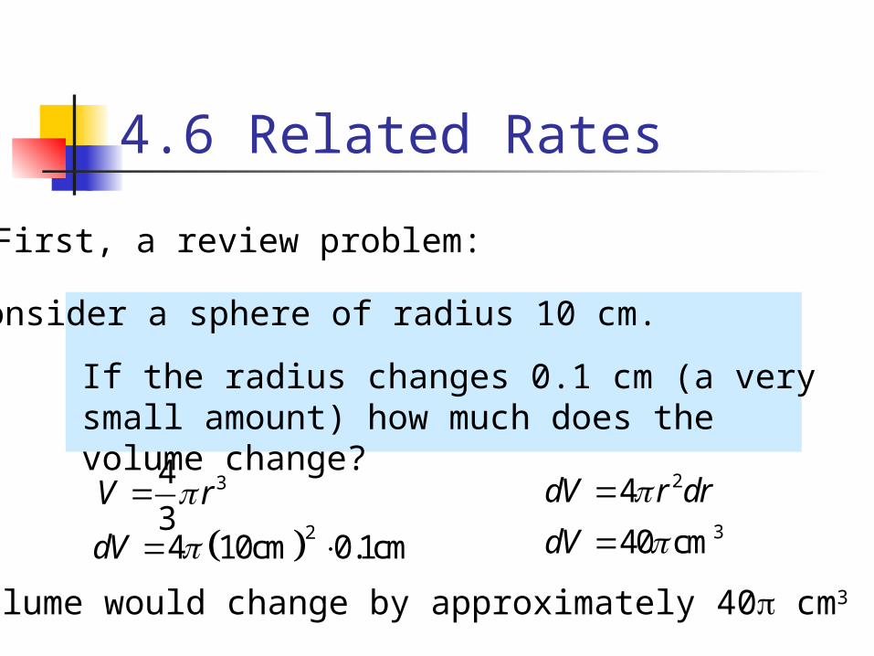
First, a review problem:
Consider a sphere of radius 10 cm.
If the radius changes 0.1 cm (a very small amount) how much does the volume change?
34
3V r 24dV r dr
24 10cm 0.1cmdV 340 cmdV
The volume would change by approximately 40 cm3 .
4.6 Related Rates
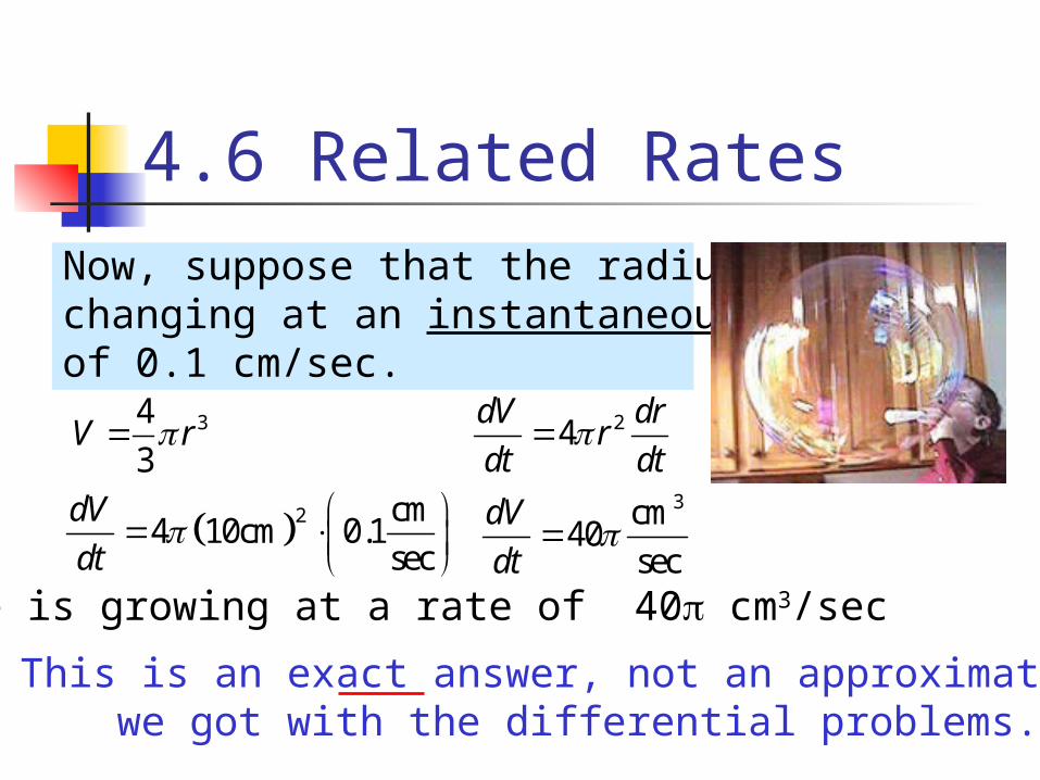
Now, suppose that the radius is changing at an instantaneous rate of 0.1 cm/sec.
34
3V r 24
dV drr
dt dt
2 cm4 10cm 0.1
sec
dV
dt
3cm40
sec
dV
dt
The sphere is growing at a rate of 40 cm3/sec .
Note: This is an exact answer, not an approximation like we got with the differential problems.
4.6 Related Rates
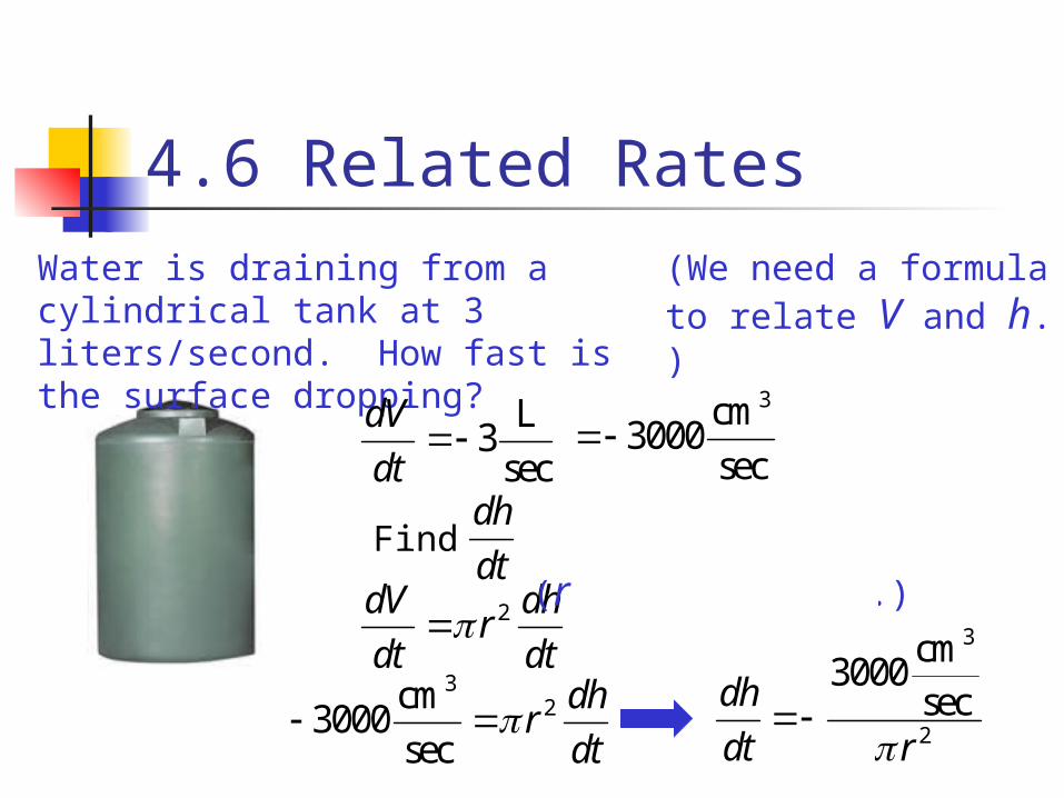
Water is draining from a cylindrical tank at 3 liters/second. How fast is the surface dropping?
L3
sec
dV
dt
3cm3000
sec
Finddh
dt2V r h
2dV dhr
dt dt
(r is a constant.)
32cm
3000sec
dhr
dt
3
2
cm3000
secdh
dt r
(We need a formula to relate V and h. )
4.6 Related Rates
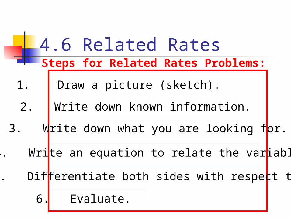
Steps for Related Rates Problems:
1. Draw a picture (sketch).
2. Write down known information.
3. Write down what you are looking for.
4. Write an equation to relate the variables.
5. Differentiate both sides with respect to t.
6. Evaluate.
4.6 Related Rates
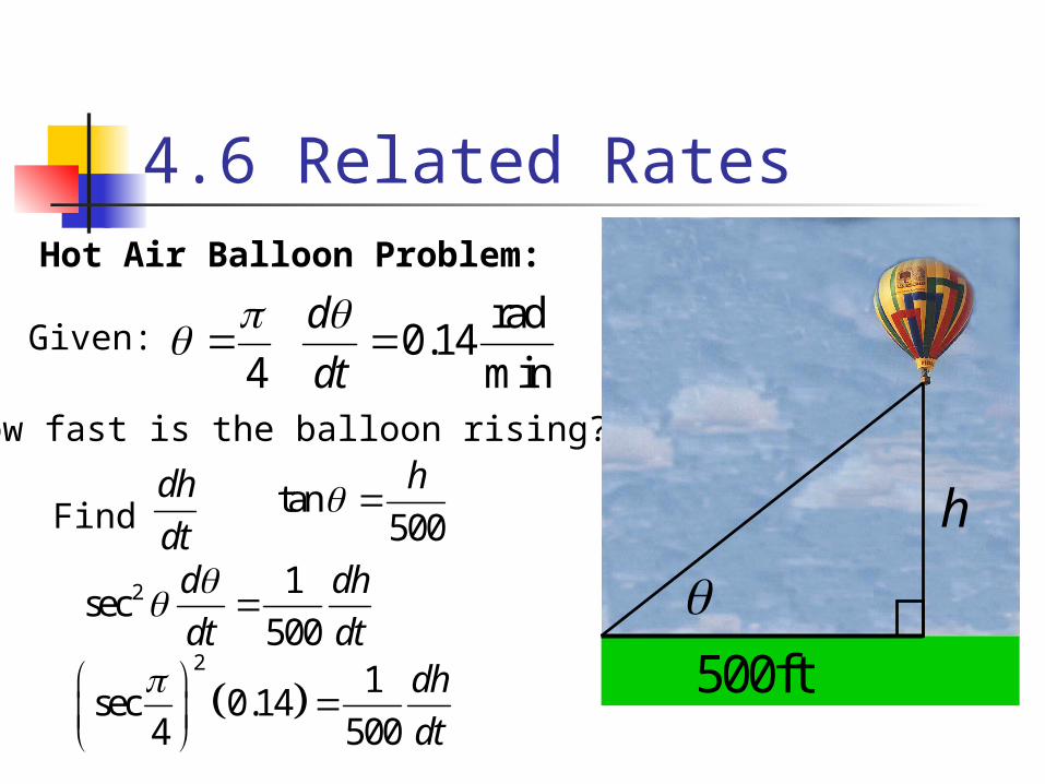
Hot Air Balloon Problem:
Given:4
rad
0.14min
d
dt
How fast is the balloon rising?
Finddh
dttan
500
h
2 1sec
500
d dh
dt dt
2
1sec 0.14
4 500
dh
dt
h
500ft
4.6 Related Rates

Hot Air Balloon Problem:
Given:4
rad
0.14min
d
dt
How fast is the balloon rising?
Finddh
dttan
500
h
2 1sec
500
d dh
dt dt
2
1sec 0.14
4 500
dh
dt
h
500ft
2
2 0.14 500dh
dt
1
12
4
sec 24
ft140
min
dh
dt
4.6 Related Rates
4x
3y
B
A
5z
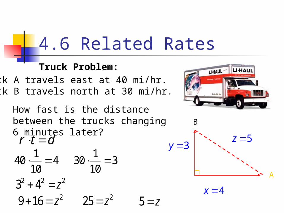
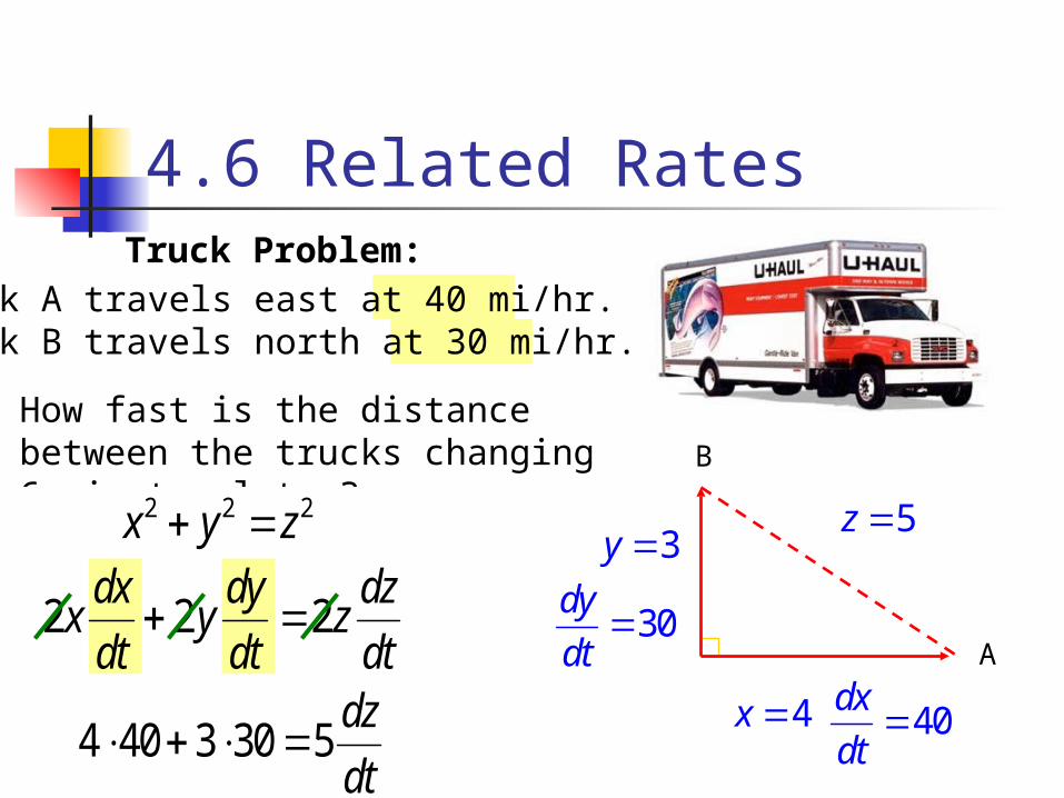
Truck Problem:Truck A travels east at 40 mi/hr.Truck B travels north at 30 mi/hr.
How fast is the distance between the trucks changing 6 minutes later?
r t d 1
40 410
130 3
10
2 2 23 4 z 29 16 z 225 z 5 z
4.6 Related Rates
4x
3y
30dy
dt
40dx
dt
B
A
5z
Truck Problem:
How fast is the distance between the trucks changing 6 minutes later?
r t d 1
40 410
130 3
10
2 2 23 4 z 29 16 z
2 2 2x y z
2 2 2dx dy dz
x y zdt dt dt
4 40 3 30 5dz
dt
Truck A travels east at 40 mi/hr.Truck B travels north at 30 mi/hr.
4.6 Related Rates
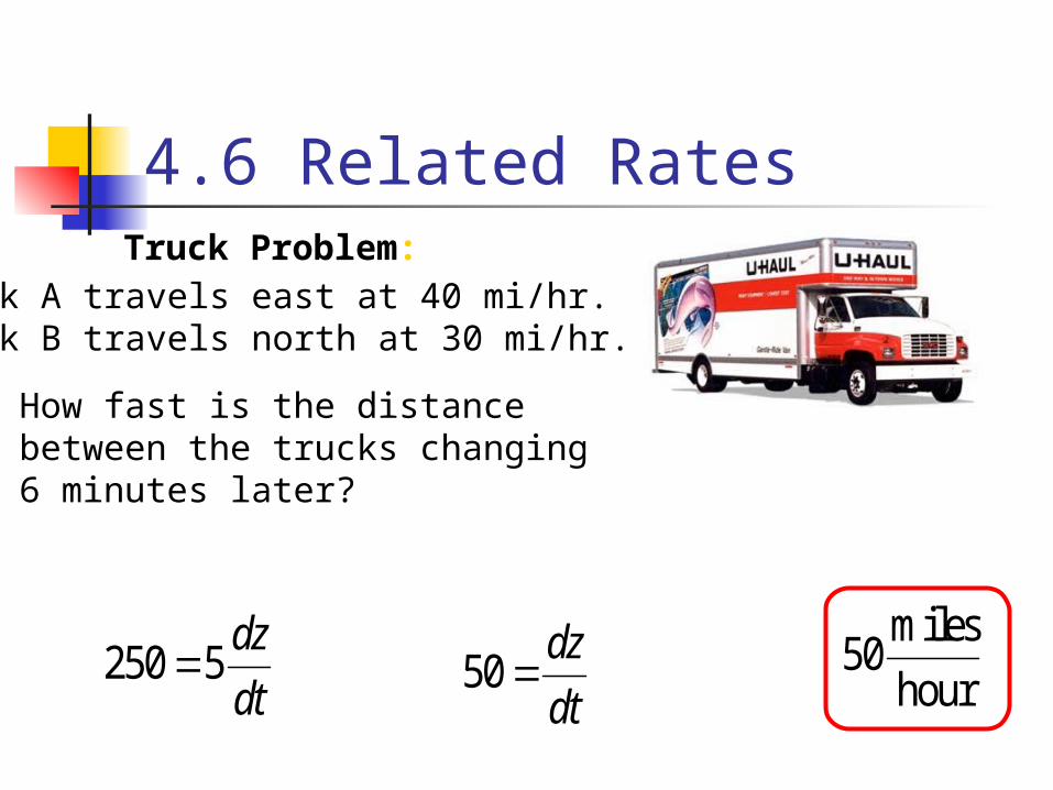
250 5dz
dt 50
dz
dt
miles50
hour
4.6 Related RatesTruck Problem:
How fast is the distance between the trucks changing 6 minutes later?
Truck A travels east at 40 mi/hr.Truck B travels north at 30 mi/hr.