abi software book - read the docs · abi software book, release 0.2-@embc13 in order to create your...
TRANSCRIPT

ABI Software BookRelease 0.2-@EMBC13
Auckland Bioengineering Institute
August 13, 2015


Contents
1 The Physiome Model Repository 31.1 PMR - an introduction . . . . . . . . . . . . . . . . . . . . . . . . . . . . . . . . . . . . . . . . 31.2 Downloading and viewing models from the Physiome Model Repository . . . . . . . . . . . . . 31.3 Working with PMR workspaces . . . . . . . . . . . . . . . . . . . . . . . . . . . . . . . . . . . 61.4 CellML Model Repository tutorial . . . . . . . . . . . . . . . . . . . . . . . . . . . . . . . . . . 131.5 Creating CellML exposures . . . . . . . . . . . . . . . . . . . . . . . . . . . . . . . . . . . . . 231.6 Creating FieldML exposures . . . . . . . . . . . . . . . . . . . . . . . . . . . . . . . . . . . . . 301.7 Embedded workspaces and their uses . . . . . . . . . . . . . . . . . . . . . . . . . . . . . . . . 351.8 CellML Curation in Legacy Repository Software . . . . . . . . . . . . . . . . . . . . . . . . . . 351.9 Using SED-ML to specify simulations . . . . . . . . . . . . . . . . . . . . . . . . . . . . . . . . 37
2 OpenCOR 392.1 Command Line Interface (CLI) . . . . . . . . . . . . . . . . . . . . . . . . . . . . . . . . . . . 392.2 Graphical User Interface (GUI) . . . . . . . . . . . . . . . . . . . . . . . . . . . . . . . . . . . 402.3 CellML annotation view plugin . . . . . . . . . . . . . . . . . . . . . . . . . . . . . . . . . . . 442.4 CellML model repository plugin . . . . . . . . . . . . . . . . . . . . . . . . . . . . . . . . . . . 552.5 CellML tools plugin . . . . . . . . . . . . . . . . . . . . . . . . . . . . . . . . . . . . . . . . . 572.6 File browser plugin . . . . . . . . . . . . . . . . . . . . . . . . . . . . . . . . . . . . . . . . . . 572.7 File organiser plugin . . . . . . . . . . . . . . . . . . . . . . . . . . . . . . . . . . . . . . . . . 602.8 Help plugin . . . . . . . . . . . . . . . . . . . . . . . . . . . . . . . . . . . . . . . . . . . . . . 662.9 Single cell view plugin . . . . . . . . . . . . . . . . . . . . . . . . . . . . . . . . . . . . . . . . 692.10 Supported platforms . . . . . . . . . . . . . . . . . . . . . . . . . . . . . . . . . . . . . . . . . 822.11 Plugin approach . . . . . . . . . . . . . . . . . . . . . . . . . . . . . . . . . . . . . . . . . . . 83
3 MAP Client 873.1 MAP Installation and Setup Guide . . . . . . . . . . . . . . . . . . . . . . . . . . . . . . . . . . 873.2 MAP Features Demonstration . . . . . . . . . . . . . . . . . . . . . . . . . . . . . . . . . . . . 893.3 MAP Tutorial - Create Workflow . . . . . . . . . . . . . . . . . . . . . . . . . . . . . . . . . . 923.4 MAP Plugins . . . . . . . . . . . . . . . . . . . . . . . . . . . . . . . . . . . . . . . . . . . . . 953.5 MAP Tutorial - Create Plugin . . . . . . . . . . . . . . . . . . . . . . . . . . . . . . . . . . . . 97
4 Developing the Virtual Physiological Human 994.1 Creating a new piece of work . . . . . . . . . . . . . . . . . . . . . . . . . . . . . . . . . . . . 994.2 Reproducing published data . . . . . . . . . . . . . . . . . . . . . . . . . . . . . . . . . . . . . 1094.3 Find an existing piece of work and extend it . . . . . . . . . . . . . . . . . . . . . . . . . . . . . 114
5 Related Software Project at the Auckland Bioengineering Institute 1195.1 Cmgui user documentation . . . . . . . . . . . . . . . . . . . . . . . . . . . . . . . . . . . . . . 1195.2 OpenCMISS user documentation . . . . . . . . . . . . . . . . . . . . . . . . . . . . . . . . . . 184
6 Glossary 209
7 Tutorial to do list 211
i

7.1 General . . . . . . . . . . . . . . . . . . . . . . . . . . . . . . . . . . . . . . . . . . . . . . . . 2117.2 Within sections . . . . . . . . . . . . . . . . . . . . . . . . . . . . . . . . . . . . . . . . . . . . 211
8 Indices and tables 2138.1 ABI research case studies . . . . . . . . . . . . . . . . . . . . . . . . . . . . . . . . . . . . . . 2138.2 About the ABI . . . . . . . . . . . . . . . . . . . . . . . . . . . . . . . . . . . . . . . . . . . . 2138.3 CAP user documentation . . . . . . . . . . . . . . . . . . . . . . . . . . . . . . . . . . . . . . . 2148.4 CM user documentation . . . . . . . . . . . . . . . . . . . . . . . . . . . . . . . . . . . . . . . 2148.5 CellML API user documentation . . . . . . . . . . . . . . . . . . . . . . . . . . . . . . . . . . . 2148.6 Exporting ip files for CM from cmgui . . . . . . . . . . . . . . . . . . . . . . . . . . . . . . . . 2148.7 Testing MathJax LaTeX support . . . . . . . . . . . . . . . . . . . . . . . . . . . . . . . . . . . 2148.8 MAP Client . . . . . . . . . . . . . . . . . . . . . . . . . . . . . . . . . . . . . . . . . . . . . . 2148.9 MAP Installation and Setup Guide . . . . . . . . . . . . . . . . . . . . . . . . . . . . . . . . . . 2268.10 PMR best practice - embedded workspaces . . . . . . . . . . . . . . . . . . . . . . . . . . . . . 2278.11 CellML Curation in Legacy Repository Software . . . . . . . . . . . . . . . . . . . . . . . . . . 2278.12 Physiome Model Repository web interface reference . . . . . . . . . . . . . . . . . . . . . . . . 229
ii

ABI Software Book, Release 0.2-@EMBC13
This book is a collection of documentation covering software used within the ABI. This includes software devel-oped internally and also other commonly used applications. The version of the book has been customised for atutorial presented at the EMBC 2013 meeting.
Contents:
Contents 1

ABI Software Book, Release 0.2-@EMBC13
2 Contents

CHAPTER 1
The Physiome Model Repository
The documentation found here is mainly aimed towards providing information to users of the Physiome ModelRepository. This includes users interested in obtaining and running models from the respository, and those whowish to add models to the repository.
If you wish to deploy an instance of the repository software, PMR Software, please see the buildout repository onGitHub.
1.1 PMR - an introduction
The Physiome Model Repository (PMR (Physiome Model Repository)) site is a web accessible repository ofmodels which includes the CellML and FieldML repositories. (Note: the PMR site is powered by software calledthe PMR Software. Usually the term PMR will be referring to the PMR site, but if clarification is needed, “PMRsite” will be used. It is also sometimes referred to as a “PMR instance”, since it is possible to create other sitesrunning the PMR Software, i.e. other instances.)
PMR relies on the distributed version control system Mercurial (Hg), which allows the repository to maintain acomplete history of all changes made to every file contained within repository workspaces. In order to use thePhysiome Model Repository, you will need to obtain a Mercurial client for your operating system, and becomefamiliar with the basic functions of Mercurial. There are many excellent resources available on the internet, suchas Mercurial, the definitive guide. Mercurial clients may be downloaded from the Mercurial website, which alsoprovides documentation on Mercurial usage. A graphical alternative to a command-line client is available forWindows, called TortoiseHg. This provides a Windows explorer integrated system for working with Mercurialrepositories.
1.2 Downloading and viewing models from the Physiome ModelRepository
There are several ways of obtaining and using models from the Physiome Model Repository, and which youchoose will depend on the way you intend to use the models. If you are simply interested in running a particularmodel and viewing the output, you can use links found on model exposure pages to get hold of the model files.There links available for a large number of models that will load the model directly into the OpenCell application,allowing you to explore simulation results with the help of a model diagram.
If you intend to use the model for further work, for example saving changes to the model or creating a new modelbased on an existing model or parts of an existing model, you should use Mercurial to obtain the files. In thisway you also obtain the complete revision history of the files, and can add to this history as you make your ownchanges.
3

ABI Software Book, Release 0.2-@EMBC13
1.2.1 Searching the repository
The Physiome Model Repository has a basic search function that can be accessed by typing search terms into thebox at the top right hand side of the page. You can use keywords such as cardiac or insulin, author names,or any other terms relevant to the models you want to find.
Fig. 1.1: The index page of the model repository provides two methods for finding models. There is a boxfor entering search terms, or you can click on categories based on model keywords to see all models in thosecategories.
If your search is yielding too many results, you may either try to narrow it down by choosing more or differentkeywords (eg. goldbeter 1991 instead of just goldbeter), or you can click the Advanced Search link justunder the search box on the results page. This will take you to a search page where you can select specific itemtypes (eg. exposures or workspaces), statuses, and other specifics.
Once you have found the model you are interested in, there are several ways you can view or download it.
1.2.2 Viewing models via the respository web interface
The most common use of the Physiome Model Repository web interface is probably to view information aboutmodels found on exposure pages, and to then download the models from these pages for simulation in a CellMLsupporting application.
4 Chapter 1. The Physiome Model Repository

ABI Software Book, Release 0.2-@EMBC13
Fig. 1.2: In this search I have chosen to only have published exposures in my results.
1.2. Downloading and viewing models from the Physiome Model Repository 5

ABI Software Book, Release 0.2-@EMBC13
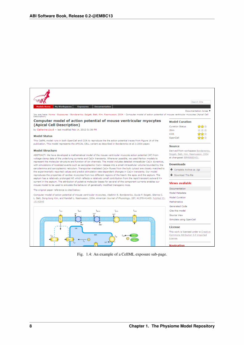
Below is an example of a CellML exposure page. It contains documentation about the model(s), a diagram of thewhat the model(s) represent, and a navigation pane that allows the user to select between available versions of themodel. Many models only have one version, but in this case there are two variants.
If you click on one of the model variant navigation links, you will be taken to a sub-page of the exposure whichwill allow you to view the actual CellML model in a number of ways.
On this page there are a number of options under a Views available panel at the right hand side.
• Documentation - displays the model documentation, already visible in the main area of the exposure page.
• Model Metadata - displays information such as the citation information, model authorship details, and PMRkeywords.
• Model Curation - displays the curation stars for the model, also visible at the top right of the page. Futureadditions to the curation system mean that there will be additional information to be displayed on this page.
• Mathematics - displays all the equations in the model in graphical form.
• Generated code - shows a page where you can view the model in a number of different languages; C,C_IDA, Fortran 77, MATLAB, and Python. You can copy the generated code directly from this page topaste into your code editor.
• Cite this model - this page provides generic information about how to cite models in the repository.
• Source View - provides a raw view of the CellML (XML) model code.
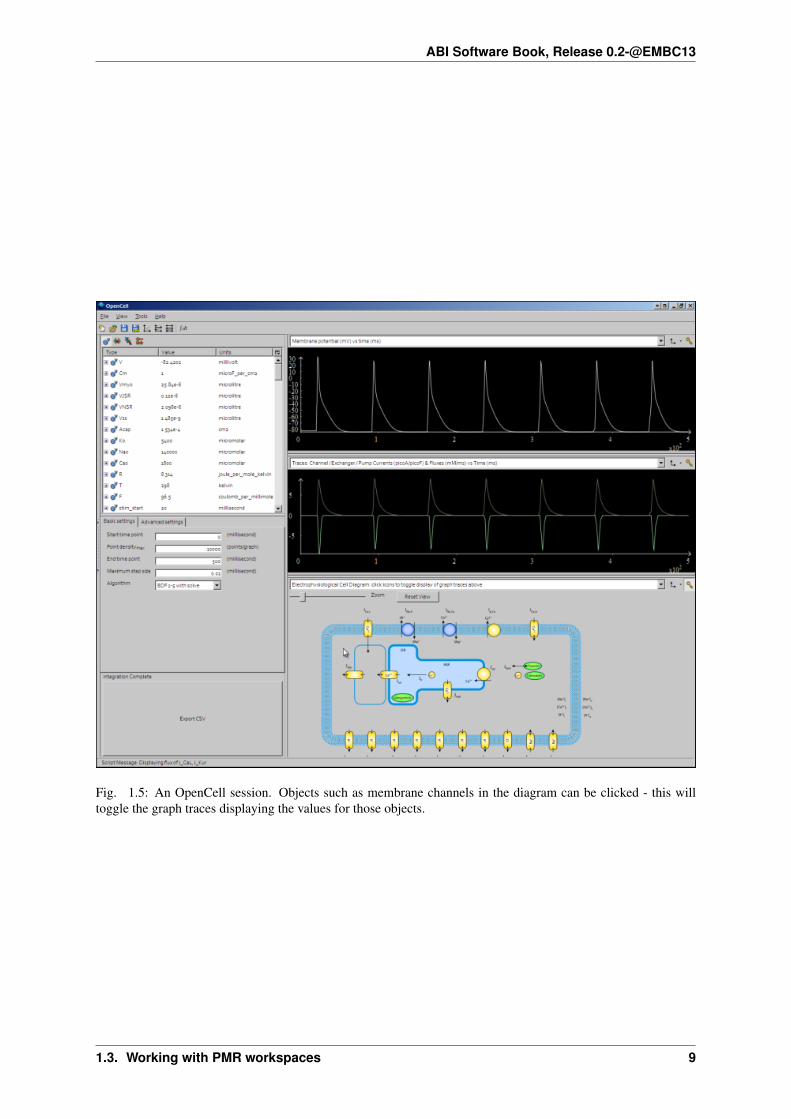
• Simulate using OpenCell - this link will download the model and open it with OpenCell if you have thesoftware installed. If the model has a session file, this will include an interactive diagram which can beclicked on to display traces of the simulation results.
The OpenCell session that is loaded when clicking on the Simulate using OpenCell link looks something like this:
1.2.3 Downloading models via Mercurial
All data in PMR are stored in workspaces and each workspace is a Mercurial repository. The most comprehensivemethod of downloading content from PMR is to clone the workspace containing the desired data. In this manneryou will have a local copy of the entire history of that data, including all provenance data, and the ability tostep back through the history of the workspace to a state that may not be available via the download links in theexposure pages discussed above. If you would like to modify the contents of workspace, making use of Mercurialwill ensure accurate provenance records are maintained as well as all the other benefits of using a version controlsystem.
As software tools like OpenCOR and MAP evolve, they will be able to hide a lot of the Mercurial details andpresent the user with a user interface suitable for their specific application areas. Directly using Mercurial is,however, currently the most powerful way to leverage the full capabilities of PMR. Instructions for working withMercurial can be found in the CellML repository tutorial.
TodoNeed to check this section on obtaining models via mercurial.
1.3 Working with PMR workspaces
Section author: David Nickerson
All models in the Physiome Model Repository exist in workspaces, which are Mercurial repositories that can beused to store any kind of file. Mercurial is a distributed version control system (DVCS).
6 Chapter 1. The Physiome Model Repository

ABI Software Book, Release 0.2-@EMBC13
Fig. 1.3: An example of a CellML exposure page.
1.3. Working with PMR workspaces 7
ABI Software Book, Release 0.2-@EMBC13
Fig. 1.4: An example of a CellML exposure sub-page.
8 Chapter 1. The Physiome Model Repository
ABI Software Book, Release 0.2-@EMBC13
Fig. 1.5: An OpenCell session. Objects such as membrane channels in the diagram can be clicked - this willtoggle the graph traces displaying the values for those objects.
1.3. Working with PMR workspaces 9
ABI Software Book, Release 0.2-@EMBC13
In order to create your own workspaces, you will first need to create a repository account by registering at mod-els.physiomeproject.org. Near the top right of the repository page there will be links labelled Log in and Register.Click on the register link, and follow the instructions.
Workspaces in the Physiome Model Repository are permanent once they are created. There is a teaching instanceof the model repository which may be used for experimenting with PMR without worrying about creating perma-nent workspaces that might have errors in them. Users accounts from the main PMR instance will be copied tothe teaching instance each time it is recreated, but users may register for an account just on the teaching instanceif they prefer. Such accounts will need to be recreated each time the teaching instance is recreated.
Note: The teaching instance of the repository is a mirror of the main repository site found athttp://models.physiomeproject.org/, running the latest development version of the PMR Software.
Any changes you make to the contents of the teaching instance are not permanent, and will be overwritten withthe contents of the main repository whenever the teaching instance is upgraded to a new PMR Software release.For this reason, you can feel free to experiment and make mistakes when pushing to the teaching instance. Pleasesubscribe to the cellml-discussion mailing list to receive notifications of when the teaching instance will be re-freshed.
See the section Migrating content to the main repository for instructions on how to migrate any content from theteaching instance to the main (permanent) Physiome Model Repository.
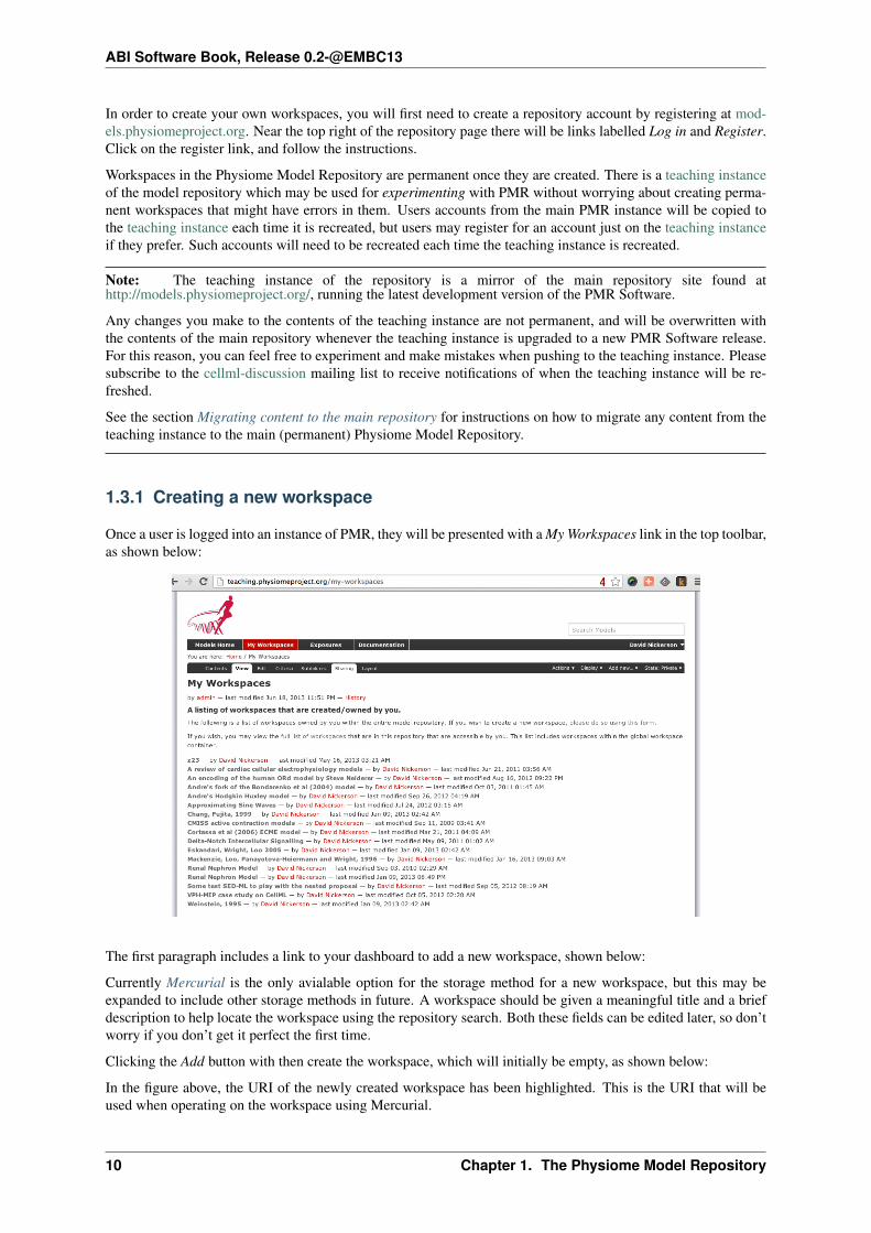
1.3.1 Creating a new workspace
Once a user is logged into an instance of PMR, they will be presented with a My Workspaces link in the top toolbar,as shown below:
The first paragraph includes a link to your dashboard to add a new workspace, shown below:
Currently Mercurial is the only avialable option for the storage method for a new workspace, but this may beexpanded to include other storage methods in future. A workspace should be given a meaningful title and a briefdescription to help locate the workspace using the repository search. Both these fields can be edited later, so don’tworry if you don’t get it perfect the first time.
Clicking the Add button with then create the workspace, which will initially be empty, as shown below:
In the figure above, the URI of the newly created workspace has been highlighted. This is the URI that will beused when operating on the workspace using Mercurial.
10 Chapter 1. The Physiome Model Repository

ABI Software Book, Release 0.2-@EMBC13
1.3. Working with PMR workspaces 11
ABI Software Book, Release 0.2-@EMBC13
1.3.2 Working with collaborators
PMR makes use of Mercurial to manage individual workspaces. Mercurial is a Distributed Version Control System(DVCS), and as such encourages collaborative development of your model, dataset, results, etc. Using Mercurial,each member of the development team is able to have their own clone of the workspace which can be kept syn-chronized with the other members of the development team, while ensuring that each team member’s contributionsare accurately recorded in the workspace history.
Once a PMR workspace has been published, any user of the repository is able to access and clone the workspace,including team members and the anonymous public. Only privileged PMR members are able to make changes tothe workspace, including pushing changes into the Mercurial repository. Private PMR workspaces, however, canonly be viewed by those PMR members that have been granted access.
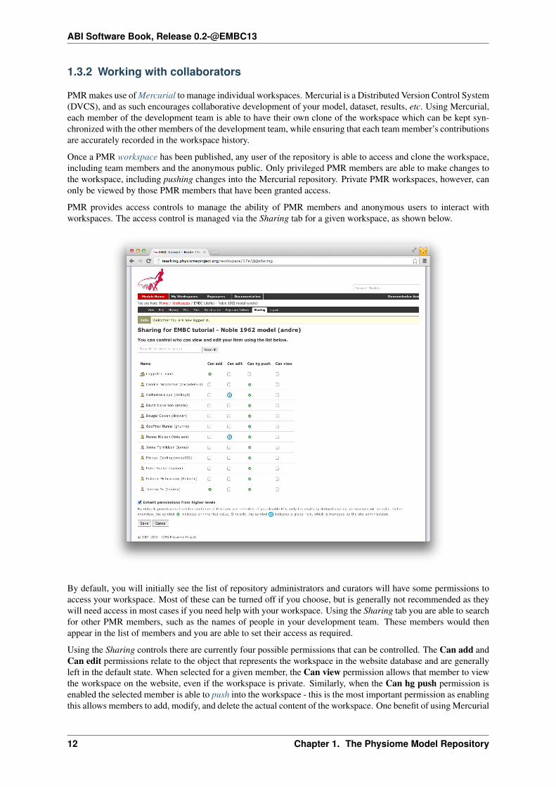
PMR provides access controls to manage the ability of PMR members and anonymous users to interact withworkspaces. The access control is managed via the Sharing tab for a given workspace, as shown below.
By default, you will initially see the list of repository administrators and curators will have some permissions toaccess your workspace. Most of these can be turned off if you choose, but is generally not recommended as theywill need access in most cases if you need help with your workspace. Using the Sharing tab you are able to searchfor other PMR members, such as the names of people in your development team. These members would thenappear in the list of members and you are able to set their access as required.
Using the Sharing controls there are currently four possible permissions that can be controlled. The Can add andCan edit permissions relate to the object that represents the workspace in the website database and are generallyleft in the default state. When selected for a given member, the Can view permission allows that member to viewthe workspace on the website, even if the workspace is private. Similarly, when the Can hg push permission isenabled the selected member is able to push into the workspace - this is the most important permission as enablingthis allows members to add, modify, and delete the actual content of the workspace. One benefit of using Mercurial
12 Chapter 1. The Physiome Model Repository

ABI Software Book, Release 0.2-@EMBC13
means that even if one of the privileged members accidentally modifies the workspace in a detrimental manner,you are able to revert the workspace back to the previous state.
When working in a collaborative team you would generally enable the Can hg push and Can view permissionsfor all team members and only enable the Can add and Can edit permissions for the team members responsiblefor the workspace presentation in the PMR website.
1.3.3 Uploading files to your workspace
The basic process for adding content to a workspace consists of the following steps:
1. Clone the workspace to your local machine.
2. Add files to cloned workspace.
3. Commit the files using a Mercurial client.
4. Push the workspace back to the repository.
An example demonstrating these steps can be found in in this tutorial step: Populate with content.
1.4 CellML Model Repository tutorial
Section author: David Nickerson, Randall Britten, Dougal Cowan
1.4.1 About this tutorial
The CellML model repository is an instance of the Physiome Model Repository (PMR) customised for CellMLmodels. PMR currently relies on the distributed version control system Mercurial (Hg), which allows the reposi-tory to maintain a complete history of all changes made to every file it contains. This tutorial demonstrates howto work with the repository using TortoiseHg, which provides a Windows explorer integrated system for workingwith Mercurial repositories.
Brief mention of the equivalent command line versions of the TortoiseHgactions will also be mentioned, so that these ideas can also be used withouta graphical client, and on Linux and similar systems. These will be denotedby boxes like this.
This tutorial requires you to have:
• A Mercurial client such as TortoiseHg or Mercurial installed
• The OpenCell CellML modelling environment
• A text editor such as Notepad++ or gedit
1.4.2 PMR concepts
PMR and the CellML model repository use a certain amount of jargon - some is specific to the repository software,and some is related to distributed version control systems (DVCSs). Below are basic explanations of some of theseterms as they apply to the repository.
Workspace A container (much like a folder or directory on your computer) to hold the files that make up a model,as well as any other files such as documentation or metadata, etc. In practical terms, each workspace is aMercurial repository.
Exposure An exposure is a publicly viewable presentation of a particular revision of a model. An exposure canpresent one or many files from your workspace, along with documentation and other information about yourmodel.
1.4. CellML Model Repository tutorial 13

ABI Software Book, Release 0.2-@EMBC13
The Mercurial DVCS has a range of terms that are useful to know, and definitions of these terms can be found inthe Mercurial glossary: http://mercurial.selenic.com/wiki/Glossary.
1.4.3 Working with the repository web interface
This part of the tutorial will teach you how to find models in the Physiome Model Repository(http://models.physiomeproject.org), how to view a range of information about those models, and how to down-load models. The first page in the repository consists of basic navigation, a link to the main model listing, a searchbox at the top right, and a list of model category links as shown below.
Fig. 1.6: The front page of the Physiome Model Repository.
Model listings
Clicking on the main model listing or any of the category listings will take you to a page displaying a list ofexposed models in that category. Click on electrophysiology for example, and a list of over 100 exposed modelsin that category will be displayed, as shown here.
Clicking on an item in the list will take you to the exposure page for that model.
Searching the repository
You can search for the model that you wish to work on by entering a search term in the box at the top right ofthe page. Many of the models in the repository are named by the first author and publication date of the paper,so a good search query might be something like goldbeter 1991. A list of the results of your search will probablycontain both workspaces and exposures - you will need to click on the workspace of the model you wish to workon. Workspaces can be identified because their links are pale blue and have no details line following the clickablelink. In the following screenshot, the first two results are workspaces, and the remainder are exposures.
Click on an exposure result to view information about the model and to get links for downloading or simulatingthe model. Click on workspaces to see the contents of the model workspace and the revision history of the model.
14 Chapter 1. The Physiome Model Repository

ABI Software Book, Release 0.2-@EMBC13
Fig. 1.7: A list of models in the electrophysiology category.
Fig. 1.8: A search results listing on the Physiome Model Repository site.
1.4. CellML Model Repository tutorial 15

ABI Software Book, Release 0.2-@EMBC13
1.4.4 Working with the repository using Mercurial
This part of the tutorial will teach you how to clone a workspace from the model repository using a Mercurialclient, create your own workspace, and then push the cloned workspace into your new workspace in the repository.We will be using a fork of an existing workspace, which provides you with a personal copy of a workspace thatyou can edit and push changes to.
Registering an account and logging in
First, navigate to the teaching instance of the Physiome Model Repository at http://teaching.physiomeproject.org/.
Note: The teaching instance of the repository is a mirror of the main repository site found athttp://models.physiomeproject.org/, running the latest development version of the PMR Software.
Any changes you make to the contents of the teaching instance are not permanent, and will be overwritten withthe contents of the main repository whenever the teaching instance is upgraded to a new PMR Software release.For this reason, you can feel free to experiment and make mistakes when pushing to the teaching instance. Pleasesubscribe to the cellml-discussion mailing list to receive notifications of when the teaching instance will be re-freshed.
See the section Migrating content to the main repository for instructions on how to migrate any content from theteaching instance to the main (permanent) Physiome Model Repository.
In order to make changes to models in the CellML repository, you must first register for an account. The Login and Register links can be found near the top right corner of the page. Your account will have the appropriateaccess privileges so that you can push any changes you have made to a model back into the repository.
Click on the Register link near the top right, and fill in the registration form. Enter your username and desiredpassword. After completing the email validation step, you can now log in to the repository.
Note: This username and password are also the credentials you use to interact with the repository via Mercurial.
Once logged in to the repository, you will notice that there is a new link in the navigation bar, My Workspaces.This is where all the workspaces you create later on will be listed. The Log in and Register links are also replacedby your username and a Log out link.
Mercurial username configuration
Important: Username setup for MercurialSince you are about to make changes, your name needs to be recorded as part of the workspace revision his-tory. When commit your changes using Mercurial, it is initially “offline” and independent of the central PMRinstance. This means that you have to set-up your username for the Mercurial client software, even though youhave registered a username on the PMR site.
You only need to do this once.
Steps for TortoiseHg:
• Right click on any file or folder in Windows Explorer, and select TortoiseHg → Global Settings.
• Select Commit and then enter your name followed by your e-mail address in “angle brackets” (i.e. less-than “<” and greater-than “>”). Actually, you can enter anything you want here, but this is the acceptedbest practice. Note that this information becomes visible publicly if the PMR instance that you push youchanges to is public.
Steps for command line:
• Edit the config text file:
– For per repository settings, the file in the repository: <repo>\.hg\hgrc
16 Chapter 1. The Physiome Model Repository

ABI Software Book, Release 0.2-@EMBC13
– System-wide settings for Linux: %USERPROFILE%\.hgrc
– System-wide settings for Windows: %USERPROFILE%\mercurial.ini
• Add the following entry:
[ui]username = Firstname Lastname <[email protected]>
Forking an existing workspace
Important: It is essential to use a Mercurial client to obtain models from the repository for editing. TheMercurial client is not only able to keep track of all the changes you make (allowing you to back-track if youmake any errors), but using a Mercurial client is the only way to add any changes you have made back into therepository.
For this tutorial we will fork an existing workspace. This creates new workspace owned by you, containing acopy of all the files in the workspace you forked including their complete history. This is equivalent to cloningthe workspace, creating a new workspace for yourself, and then pushing the contents of the cloned workspace intoyour new workspace.
Forking a workspace can be done using the Physiome Model Repository web interface. The first step is tofind the workspace you wish to fork. We will use the Beeler, Reuter 1977 workspace which can be found at:http://teaching.physiomeproject.org/workspace/beeler_reuter_1977.
Now click on the fork option in the toolbar, as shown below.
You will be asked to confirm the fork action by clicking the Fork button. You will then be shown the page for yourforked workspace.
Cloning your forked workspace
In order to make changes to your workspace, you have to clone it to your own computer. In order to do this, copythe URI for mercurial clone/pull/push as shown below:
In Windows explorer, find the folder where you want to create the clone of the workspace. Then right click tobring up the context menu, and select TortoiseHG → Clone as shown below:
1.4. CellML Model Repository tutorial 17

ABI Software Book, Release 0.2-@EMBC13
Fig. 1.9: Copying the URI for cloning your workspace.
18 Chapter 1. The Physiome Model Repository

ABI Software Book, Release 0.2-@EMBC13
Paste the copied URL into the Source: area and then click the Clone button. This will create a folder calledbeeler_reuter_1977_tut that contains all the files and history of your forked workspace. The folder willbe created inside the folder in which you instigated the clone command.
Command line equivalent
hg clone [URI]
You will need to enter your username and password to clone the workspace, as the fork will be set to private whenit is created.
The repository will be cloned within the current directory of your command line window.
Making changes to workspace contents
Your cloned workspace is now ready for you to edit the model file and make a commit each time you want to savethe changes you have made. As an example, open the model file in your text editor and remove the paragraphwhich describes validation errors from the documentation section, as shown below:
Save the file. If you are using TortoiseHg, you will notice that the icon overlay has changed to a red exclamationmark. This indicates that the file now has uncommitted changes.
Committing changes
If you are using TortoiseHg, bring up the shell menu for the altered file and select TortoiseHg → Hg Commit.A window will appear showing details of the changes you are about to commit, and prompting for a commitmessage. Every time you commit changes, you should enter a useful commit message with information aboutwhat changes have been made. In this instance, something like “Removed the paragraph about validation errorsfrom the documentation” is appropriate.
Click on the Commit button at the far left of the toolbar. The icon overlay for the file will now change to a greentick, indicating that changes to the file have been committed.
Command line equivalent
hg commit -m "Removed the paragraph about validation errors from the documentation"
Pushing changes to the repository
Your cloned workspace on your local machine now has a small history of changes which you wish to push intothe repository.
Right click on your workspace folder in Windows explorer, and select TortoiseHg → Hg Synchronize from theshell menu. This will bring up a window from which you can manage changes to the workspace in the repository.Click on the Push button in the toolbar, and enter your username and password when prompted.
Command line equivalent
1.4. CellML Model Repository tutorial 19

ABI Software Book, Release 0.2-@EMBC13
20 Chapter 1. The Physiome Model Repository

ABI Software Book, Release 0.2-@EMBC13
hg push
Now navigate to your workspace and click on the history toolbar button. This will show entries under the Mostrecent changes, complete with the commit messages you entered for each commit, as shown below:
1.4.5 Create an exposure
As explained earlier, an exposure aims to bring a particular revision to the attention of users who are browsing andsearching the repository.
There are two ways of making an exposure - creating a new exposure from scratch, or “Rolling over” an exposure.Rolling over is used when a workspace already has an existing exposure, and the updates to the workspace havenot fundamentally changed the structure of the workspace. This means that all the information used in makingthe previous exposure is still valid for making a new exposure of a more recent revision of the workspace. Strictlyspeaking, an exposure can be rolled over to an older revision as well, but this is not the usual usage.
As you are working in a forked repository, you will need to create a new exposure from scratch. To learn how tocreate exposures, please refer to Creating CellML exposures.
1.4.6 Migrating content to the main repository
As noted above, the teaching instance used in this tutorial is not suitable for permanent storage of your work.One of the advantages of using a distributed version control system to manage PMR workspaces is that it isstraightforward to move the entire workspace, including the full history and provenance record, from one locationto another. Recent releases of PMR Software have also provided the feature to export exposures so that they canthen be imported into another PMR Software instance.
If you would like to move your work from the teaching instance of the model repository into a new workspace onthe main repository (or from any PMR Software instance to another one), you should follow these steps:
1. Ensure that you have pushed all your commits to the source instance;
2. Create the new workspace in the destination repository;
1.4. CellML Model Repository tutorial 21

ABI Software Book, Release 0.2-@EMBC13
3. Navigate to the workspace created and choose the synchronize action from the workspace toolbar, as shownbelow.
4. Fill in the URI of your workspace on the source instance (e.g.,http://models.physiomeproject.org/w/andre/cortassa-ECME-2006)
5. Click the Synchronize button.
In a similar manner, you are able to copy exposures you might have made on the teaching instance over to themain repository, or from the main to the teaching instance if you want to test things out. Follow these steps tomigrate an exposure from one repository to another.
1. Navigate to the exposure you would like to migrate in the source repository.
2. Choose the wizard item from the toolbar as shown below.
3. In the destination repository, navigate to the desired revision of the (published) workspace and choose theCreate exposure action as described in the directions for creating an exposure from scratch
4. Rather than building a new exposure, choose the Exposure Import via URI tab in the exposure creationwizard, as shown below.
5. Copy and paste the URI from the source exposure wizard, highlighted above, into the Exposure Export URIfield in the exposure creation wizard shown above.
22 Chapter 1. The Physiome Model Repository

ABI Software Book, Release 0.2-@EMBC13
6. Click the Add button. This will take you back to the standard exposure build page, but now with all thefields pre-populated from the source exposure.
7. Navigate to the bottom of the page and click the Build button to actually build the exposure pages. You arefree to reconfigure the exposure if desired, some help is available for this if needed.
1.5 Creating CellML exposures
Section author: Dougal Cowan
CellML models in the Physiome Model Repository are presented through exposures. An exposure is a view of aparticular revision of a workspace, and is quite flexible in terms of what it can present. A workspace may containone or more models, and any number of models may be presented in a single exposure. Exposures generally takethe form of some documentation about the model(s), a range of ways of looking at the model(s) or their metadata,and links to download the model(s).
The example below shows the main exposure page for the Bondarenko et al. 2004 workspace. This workspacecontains two models, which can be viewed via the Navigation pane on the right hand side of the page.
If you click on one of the model navigation links, it will take you to the page for that particular model. Ex-posures most often present a single model, although they can present any number of models, each with its owndocumentation and views.
Most of the CellML exposures in the repository are currently of this type, with a main documentation pagecontaining navigation links to the model or models themselves.
The model pages have links that enable the user to do things like view the model equations, look at the citationinformation, or run the model as an interactive session using the OpenCell application. These links are found inthe pane titled Views available on the right hand side of the page.
This tutorial contains instructions on how to create one of these standard CellML exposures, as well as informationabout how to create other alternative types of exposure.
1.5.1 Creating standard CellML exposures
Note: In order to create an exposure of a workspace, the workspace must be published. You will need to submityour workspace for publication and await review. It is not possible to create exposures in private workspaces.
1.5. Creating CellML exposures 23

ABI Software Book, Release 0.2-@EMBC13
Fig. 1.10: Example of an exposure page
24 Chapter 1. The Physiome Model Repository

ABI Software Book, Release 0.2-@EMBC13
Fig. 1.11: Example of a model exposure page
1.5. Creating CellML exposures 25

ABI Software Book, Release 0.2-@EMBC13
In this example I will use a fork of the the Beeler Reuter 1977 workspace. Creating a fork of a workspace createsa clone of that workspace that you own, and can push changes to. You can fork any publicly available workspacein the Physiome Model Repository. For more information on this feature of PMR, refer to the information onfeatures or collaboration, or see the relevant section of the tutorial.
At this point you will need to submit the workspace for publication, using the state: menu at the top right of theworkspace view page.
Fig. 1.12: The state menu is used to submit objects such as workspaces for publication. Submitted itemswill be reviewed by site administrators and then published.
You will need to wait for your workspace to be made public before you can carry on and create an exposure ofyour workspace.
Choose the revision to expose
As an exposure is created to present a particular revision of a workspace, the first thing to do is to navigate to thatrevision. To do this, first find the workspace - if this is your own workspace, you can click on the My Workspacesbutton in the navigation bar of the repository and find the workspace of interest in the listing displayed. Afternavigating to your workspace, click on the history button in the menu bar.
Fig. 1.13: The revision history of a fork of the Beeler Reuter 1977 workspace
Now you can select the revision of the workspace you wish to expose by clicking on the manifest of that revision.Usually you will want to expose the latest revision, which appears at the top of the list.
After selecting the revision you wish to expose, click on the workspace actions menu at the far right end of themenu bar and select create exposure.
26 Chapter 1. The Physiome Model Repository

ABI Software Book, Release 0.2-@EMBC13
Fig. 1.14: Selecting the manifest of the revision to expose
Building the exposure
Selecting the create exposure option in the menu bar will bring you to the first page of the exposure wizard. Thisweb interface allows you to select the model files, documentation files, and settings that will be used to create theexposure.
The initial page of the exposure creation wizard allows you to select the main documentation file and the first modelfile. Select the HTML annotator option and the HTML documentation file for the workspace in the Exposure mainview section. For the New Exposure File Entry section, choose the CellML file you wish to expose, and selectCellML as the file type.
Fig. 1.15: Selecting the main documentation and the first CellML model file
Note: Documentation should be written in HTML format. Some previous users of the CellML repository may befamiliar with the tmpdoc style documentation, which has be deprecated. For an example of what a fairly standardHTML documentation file might look like, take a look at the documentation for the Beeler Reuter 1977 model.
1.5. Creating CellML exposures 27

ABI Software Book, Release 0.2-@EMBC13
Once you have selected the documentation and model files and their types, click on the Add button. This will takeyou to the next step of the wizard, where you can select various options for the model you have chosen to expose,and will allow you to add further model files to the exposure if desired.
The wizard shows a subgroup for each CellML file to be included in the exposure. For each CellML file, selectthe following options:
• Documentation
– Documentation file - select the HTML file created to document the model
– View generator - select HTML annotator option
• Basic Model Curation
– Curation flags - CellML model repository curators may select flags according to the status of themodel
• License and Citation
– File/Citation format - select CellML RDF metadata to automatically generate a citation page usingthe model RDF
– License - select Creative Commons Attributions 3.0 Unported
• Source Viewer
– Language Type - select xml
• OpenCell Session Link
– Session File - select the session.xml if it has been created
After selecting the subgroup options, you need to click the Update button to set the chosen options for the exposurebuilder. If you do not update the subgroup, the options you selected will be replaced by the default options whenyou click Build.
For exposures where you wish to expose multiple models, click on the Add file button at this stage to create anothersubgroup. You can then use this to set up all the same options listed above for the additional model file. Rememberto click Update when you have completed selecting the options for each subgroup before adding another subgroup.
After setting all the options for the models you wish to expose, click on the Build button. The repository softwarewill then create the exposure pages and display the main page of the exposure.
In order to make the exposure visible and searchable, you will need to publish it. You can choose to submit yourexposure for review, or if you have sufficient privileges you can publish it directly.
1.5.2 Other types of exposure
Because the exposure builder uses HTML documentation, it is possible to create customized types of exposurethat differ from the standard type shown above. For example, you might want to create an exposure that simplydocuments and provides links to models in a PMR workspace that are encoded in languages other than CellML.You can also use the HTML documentation to provide tutorials or other documents, with resources stored in theworkspace and linked to from the HTML.
Examples of other exposure types:
• Andre’s Hodgkin & Huxley CellML tutorial
• Testing nested SED-ML proposals with CellML
• Aslanidi et al. cardiac models encoded in C
1.5.3 Making an exposure using “roll-over”
As explained earlier, an exposure aims to bring a particular revision to the attention of users who are browsing andsearching the repository.
28 Chapter 1. The Physiome Model Repository

ABI Software Book, Release 0.2-@EMBC13
Fig. 1.16: Selecting options for the model file subgroup
Fig. 1.17: Publish your exposure to make it visible to others.
1.5. Creating CellML exposures 29
ABI Software Book, Release 0.2-@EMBC13
“Rolling over” an exposure is the method used when a workspace already has an existing exposure, and theupdates to the workspace have not fundamentally changed the structure of the workspace. This means that allthe information used in making the previous exposure is still valid for making a new exposure of a more recentrevision of the workspace. Strictly speaking, an exposure can be rolled over to an older revision as well, but thisis not the usual usage.
Note: A forked workspace contains all of the revision history of the workspace it was created from, but does notcontain any of the exposures that existed for the original workspace. You will always need to create an exposurefrom scratch in newly forked repositories.
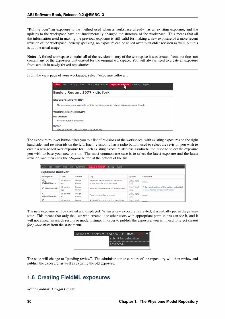
From the view page of your workspace, select “exposure rollover”.
The exposure rollover button takes you to a list of revisions of the workspace, with existing exposures on the righthand side, and revision ids on the left. Each revision id has a radio button, used to select the revision you wish tocreate a new rolled over exposure for. Each existing exposure also has a radio button, used to select the exposureyou wish to base your new one on. The most common use case is to select the latest exposure and the latestrevision, and then click the Migrate button at the bottom of the list.
The new exposure will be created and displayed. When a new exposure is created, it is initially put in the privatestate. This means that only the user who created it or other users with appropriate permissions can see it, and itwill not appear in search results or model listings. In order to publish the exposure, you will need to select submitfor publication from the state menu.
The state will change to “pending review”. The administrator or curators of the repository will then review andpublish the exposure, as well as expiring the old exposure.
1.6 Creating FieldML exposures
Section author: Dougal Cowan
30 Chapter 1. The Physiome Model Repository
ABI Software Book, Release 0.2-@EMBC13
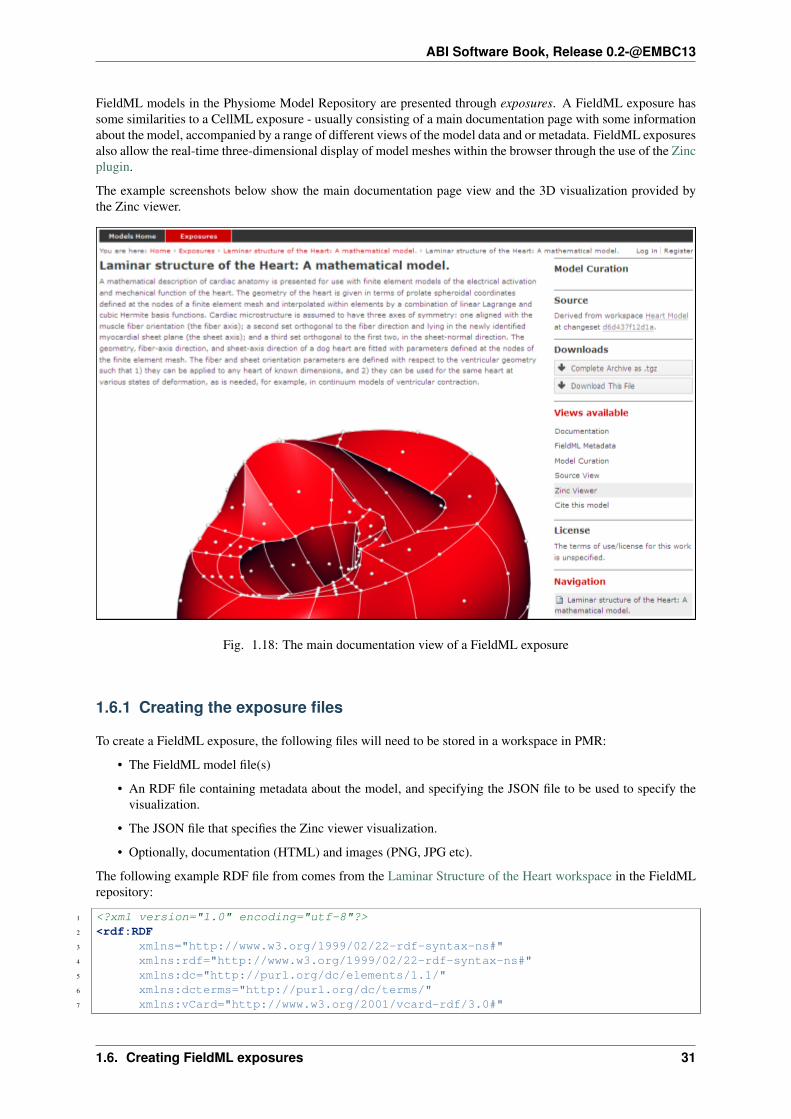
FieldML models in the Physiome Model Repository are presented through exposures. A FieldML exposure hassome similarities to a CellML exposure - usually consisting of a main documentation page with some informationabout the model, accompanied by a range of different views of the model data and or metadata. FieldML exposuresalso allow the real-time three-dimensional display of model meshes within the browser through the use of the Zincplugin.
The example screenshots below show the main documentation page view and the 3D visualization provided bythe Zinc viewer.
Fig. 1.18: The main documentation view of a FieldML exposure
1.6.1 Creating the exposure files
To create a FieldML exposure, the following files will need to be stored in a workspace in PMR:
• The FieldML model file(s)
• An RDF file containing metadata about the model, and specifying the JSON file to be used to specify thevisualization.
• The JSON file that specifies the Zinc viewer visualization.
• Optionally, documentation (HTML) and images (PNG, JPG etc).
The following example RDF file from comes from the Laminar Structure of the Heart workspace in the FieldMLrepository:
1 <?xml version="1.0" encoding="utf-8"?>2 <rdf:RDF3 xmlns="http://www.w3.org/1999/02/22-rdf-syntax-ns#"4 xmlns:rdf="http://www.w3.org/1999/02/22-rdf-syntax-ns#"5 xmlns:dc="http://purl.org/dc/elements/1.1/"6 xmlns:dcterms="http://purl.org/dc/terms/"7 xmlns:vCard="http://www.w3.org/2001/vcard-rdf/3.0#"
1.6. Creating FieldML exposures 31

ABI Software Book, Release 0.2-@EMBC13
Fig. 1.19: The main Zinc viewer view of the same FieldML exposure
32 Chapter 1. The Physiome Model Repository

ABI Software Book, Release 0.2-@EMBC13
8 xmlns:pmr2="http://namespace.physiomeproject.org/pmr2#">9 <rdf:Description rdf:about="">
10 <dc:title>11 Laminar structure of the Heart: A mathematical model.12 </dc:title>13 <dc:creator>14 <rdf:Seq>15 <rdf:li>LeGrice, I.J.</rdf:li>16 <rdf:li>Hunter, P.J.</rdf:li>17 <rdf:li>Smaill, B.H.</rdf:li>18 </rdf:Seq>19 </dc:creator>20 <dcterms:bibliographicCitation>21 American Journal of Physiology 272: H2466-H2476, 1997.22 </dcterms:bibliographicCitation>23 <dcterms:isPartOf rdf:resource="info:pmid/9176318"/>24 <pmr2:annotation rdf:parseType="Resource">25 <pmr2:type26 rdf:resource="http://namespace.physiomeproject.org/pmr2/note#json_zinc_viewer"/>27 <pmr2:fields>28 <rdf:Bag>29 <rdf:li rdf:parseType="Resource">30 <pmr2:field rdf:parseType="Resource">31 <pmr2:key>json</pmr2:key>32 <pmr2:value>heart.json</pmr2:value>33 </pmr2:field>34 </rdf:li>35 </rdf:Bag>36 </pmr2:fields>37 </pmr2:annotation>38 </rdf:Description>39 </rdf:RDF>
This file provides citation metadata and a reference to the resource that specifies the Zinc viewer JSON file whichwill be used to describe the 3D visualisation of the FieldML model. The file breaks down into three main sections:
• Lines 3-8, namespaces used.
• Lines 10-23, citation metadata.
• Lines 24-37, resource description. Used to specify the JSON file that specifies the visualisation.
Example of the JSON file from the same (Laminar Structure of the Heart) workspace:
1 {2 "View" : [3 {4 "camera" : [9.70448, -288.334, -4.43035],5 "target" : [9.70448, 6.40667, -4.43035],6 "up" : [-1, 0, 0],7 "angle" : 408 }9 ],
10 "Models": [11 {12 "files": [13 "heart.xml"14 ],15 "externalresources": [16 "heart_mesh.connectivity",17 "heart_mesh.node.coordinates"18 ],19 "graphics": [20 {
1.6. Creating FieldML exposures 33

ABI Software Book, Release 0.2-@EMBC13
21 "type": "surfaces",22 "ambient" : [0.4, 0, 0.9],23 "diffuse" : [0.4, 0,0.9],24 "alpha" : 0.3,25 "xiFace" : "xi3_1",26 "coordinatesField": "heart.coordinates"27 },28 {29 "type": "surfaces",30 "ambient" : [0.3, 0, 0.3],31 "diffuse" : [1, 0, 0],32 "specular" : [0.5, 0.5, 0.5],33 "shininess" : 0.5,34 "xiFace" : "xi3_0",35 "coordinatesField" : "heart.coordinates"36 },37 {38 "type": "lines",39 "coordinatesField" : "heart.coordinates"40 }41 ],42 "elementDiscretization" : 8,43 "region_name" : "heart",44 "group": "Structures",45 "label": "heart",46 "load": true47 }48 ]49 }
• Lines 2-8, sets up the camera or viewpoint for the initial Zinc viewer display.
• Lines 12-18, specifies the FieldML model files
• Lines 19-41, set up the actual visualisations of the mesh - in this case, two different surfaces and a set oflines.
• Lines 42-46, specify global visualisation settings.
For more information on these settings, please see the cmgui documentation.
Note: The specifics of these RDF and JSON files are a work in progress, and may change with each new versionof the Zinc viewer plugin or the PMR software.
1.6.2 Creating the exposure in the Physiome Model Repository
First you will need to create a workspace to put your model in, following the process outlined in the document onworking with workspaces.
• Upload your FieldML model files and Zinc viewer specification files.
• Find revision of workspace you wish to expose and create exposure
Exposure wizard procedure
View generator as per CellML; select HTML annotator and HTML doc file
New exposure file entry: select .rdf file and select FieldML (JSON) type. Click Add.
Documentation file - same as above Curation flags - none (should be removed?) No other settings
Click Update.
34 Chapter 1. The Physiome Model Repository

ABI Software Book, Release 0.2-@EMBC13
Click Build.
To see the 3D visualisation, you will need to have the latest Zinc plugin installed.
1.7 Embedded workspaces and their uses
Section author: David Nickerson
TodoThis section needs more work.
Workspaces in PMR are currently implemented as Mercurial repositories. One Mercurial feature that is quiteuseful in the context of the PMR is nested repositories. Using the more general PMR concepts, we term suchnesting as embedded workspaces.
Embedded workspaces:
• are intended to manage the separation of modules which are integrated to create a model;
• facilitate the sharing and reuse of model components independently from the source model;
• enable the development of the modules to proceed independently, thus the version of the workspaces em-bedded is also tracked; and
• allow authors to make use of relative URIs when linking between data resources providing a file systemagnostic method to describe complex module relationships in a portable manner.
Workspaces can be embedded at a specific revision or set to track the most recent revision of the source workspace.Changes made to the source workspace will not affect any embedding workspace until the author explicitly choosesto update the embedded workspace. This provides the author with the opportunity to review the changesets andmake an informed decision regarding alterations to embedded revisions. Any alterations in the specific revisionof an embedded workspace is data captured in a changeset in the embedding workspace – thus providing a clearprovenance record of the entire dataset in the workspace.
1.7.1 Uses
1.7.2 Best practice
See also the recommendations from the Mercurial project.
1.8 CellML Curation in Legacy Repository Software
As PMR contains much of the data ported over from the legacy software products that powered the CellML ModelRepository, the curation system from that system was ported to PMR verbatim. This document describing thecuration aspect of the repository is derived from documentation on the CellML site.
1.8.1 CellML Model Curation: the Theory
The basic measure of curation in a CellML model is described by the curation level of the model document. Wehave defined four levels of curation:
• Level 0: not curated.
• Level 1: the CellML model is consistent with the mathematics in the original published paper.
1.7. Embedded workspaces and their uses 35

ABI Software Book, Release 0.2-@EMBC13
• Level 2: the CellML models has been checked for (i) typographical errors, (ii) consistency of units, (iii) thatall parameters and initial conditions are defined, (iv) that the model is not over-constrained, in the sense thatit contains equations or initial values which are either redundant or inconsistent, and (v) that running themodel in an appropriate simulation environment reproduces the results published in the original paper.
• Level 3: the model is checked for the extent to which it satisfies physical constraints such as conservation ofmass, momentum, charge, etc. This level of curation needs to be conducted by specialised domain experts.
1.8.2 CellML Model Curation: the Practice
Our ultimate aim is to complete the curation of all the models in the repository, ideally to the level that theyreplicate the results in the published paper (level 2 curation status). However, we acknowledge that for somemodels this will not be possible. Missing parameters and equations are just one limitation; at this point it shouldalso be emphasised that the process of curation is not just about “fixing the CellML model” so that it runs incurrently available tools. Occasionally it is possible for a model to be expressed in valid CellML, but not yet ableto be solved by CellML tools. An example is the seminal Saucerman et al. 2003 model, which contains ODEsas well as a set of non-linear algebraic equations which need to be solved simultaneously. The developers of theCellML editing and simulation environment OpenCell are currently working on addressing these requirements.
The following steps describe the process of curating a CellML model:
• Step 1: the model is run through OpenCell and COR. COR in particular is a useful validation tool. It ren-ders the MathML in a human readable format making it much easier to identify any typographical errorsin the model equations. COR also provides a comprehensive error messaging system which identifies ty-pographical errors, missing equations and parameters, and any redundancy in the model such as duplicatedvariables or connections. Once these errors are fixed, and assuming the model is now complete, we com-pare the CellML model equations with those in the published paper, and if they match, the CellML modelis awarded a single star - or level 1 curation status.
• Step 2: Assuming the model is able to run in OpenCell and COR, we then go onto compare the CellMLmodel simulation output from COR and OpenCell with the published results. This is often a case of compar-ing the graphical outputs of the model with the figures in the published paper, and is currently a qualitativeprocess. If the simulation results from the CellML model and the original model match, the CellML modelis awarded a second star - or level 2 curation status.
• Step 3: if, at the end of this process, the CellML model is still missing parameters or equations, or weare unable to match the simulation results with the published paper, we seek help from the original modelauthor. Where possible, we try to obtain the original model code, and this often plays an invaluable role infixing the CellML model.
• Step 4: Sometimes we have been able to engage the original model author further, such that they take overthe responsibility of curating the CellML model themselves. Such models include those published by MikeCooling and Franc Sachse. In these instances the CellML model is awarded a third star - or level 3 curationstatus. While this is laudable, ideally we would like to take the curation process one step further, such thatlevel 3 curation should be performed by a domain expert who is not the author of the original publication(i.e., peer review). This expert would then check the CellML model meets the appropriate constraints andexpectations for a particular type of model.
A point to note is that levels 1 and 2 of the CellML model curation status may be mutually exclusive - in ourexperience, it is rare for a paper describing a model to contain no typographical errors or omissions. In thissituation, Version 1 of a CellML model usually satisfies curation level 1 in that it reflects the model as it is describedin the publication - errors included, while subsequent versions of the CellML model break the requirements formeeting level 1 curation in order to meet the standards of level 2. Taking this idea further, this means that a modelwith 2 yellow stars doesn’t necessarily meet the requirements of level 1 curation but it does meet the requirementsof level 2. Hopefully this conflict will be resolved when we replace the current star system with a more meaningfulset of curation annotations.
Ultimately, we would like to encourage the scientific modeling community - including model authors, journalsand publishing houses - to publish their models in CellML code in the CellML model repository concurrent withthe publication of the printed article. This will eliminate the need for code-to-text-to-code translations and thusavoid many of the errors which are introduced during the translation process.
36 Chapter 1. The Physiome Model Repository

ABI Software Book, Release 0.2-@EMBC13
1.8.3 CellML Model Simulation: the Theory and Practice
As part of the process of model curation, it is important to know what tools were used to simulate (run) the modeland how well the model runs in a specific simulation environment. In this case, the theory and the practice areessentially the same thing, and carry out a series of simulation steps which then translate into a confidence levelas part of a simulator’s metadata for each model. The four confidence levels are defined as:
• Level 0: not curated (no stars);
• Level 1: the model loads and runs in the specified simulation environment (1 star);
• Level 2: the model produces results that are qualitatively similar to those previously published for the model(2 stars);
• Level 3: the model has been quantitatively and rigorously verified as producing identical results to theoriginal published model (3 stars).
Note: The teaching instance of the repository is a mirror of the main repository site found athttp://models.physiomeproject.org/, running the latest development version of the PMR Software.
Any changes you make to the contents of the teaching instance are not permanent, and will be overwritten withthe contents of the main repository whenever the teaching instance is upgraded to a new PMR Software release.For this reason, you can feel free to experiment and make mistakes when pushing to the teaching instance. Pleasesubscribe to the cellml-discussion mailing list to receive notifications of when the teaching instance will be re-freshed.
See the section Migrating content to the main repository for instructions on how to migrate any content from theteaching instance to the main (permanent) Physiome Model Repository.
1.9 Using SED-ML to specify simulations
Section author: Dougal Cowan
Hopefully PMR will support SED-ML simulations as part of the CellML views.
Todo• Update all PMR documentation to reflect workspace ID changes and user workspace changes, if they go
ahead.
• Get embedded workspaces doc written.
• Get some best practice docs written.
1.9. Using SED-ML to specify simulations 37

ABI Software Book, Release 0.2-@EMBC13
38 Chapter 1. The Physiome Model Repository

CHAPTER 2
OpenCOR
OpenCOR is an open source, cross-platform and CellML-based modelling environment. The following documen-tation refers to the 2013-06-22 version of OpenCOR, for which supported platforms can be found here. Thisversion of OpenCOR can be downloaded from the tutorial download page.
OpenCOR provides two types of user interfaces:
2.1 Command Line Interface (CLI)
Note: The CLI version of OpenCOR currently offers a limited number of features. You might therefore want touse its Graphical User Interface (GUI) version instead.
2.1.1 Help
$ ./OpenCOR -hUsage: OpenCOR [-a|--about] [-c|--command [<plugin>::]<command> <options>] [-h|--help] [-p|--plugins] [-v|--version] [<files>]-a, --about Display some information about OpenCOR-c, --command Send a command to one or all the plugins-h, --help Display this help information-p, --plugins Display the list of plugins-v, --version Display the version of OpenCOR
2.1.2 Version
$ ./OpenCOR -vOpenCOR [2013-06-22] (32-bit)
2.1.3 About
$ ./OpenCOR -aOpenCOR [2013-06-22] (32-bit)GNU/Linux 3.5.0-34-genericCopyright 2011-2013
OpenCOR is a cross-platform CellML-based modelling environment which can beused to organise, edit, simulate and analyse CellML files.
39

ABI Software Book, Release 0.2-@EMBC13
2.1.4 Plugins
$ ./OpenCOR -pThe following plugin is loaded:- CellMLTools: a plugin to access various CellML-related tools.
2.1.5 Command
$ ./OpenCOR -c helpCommands supported by CellMLTools:
* Display the commands supported by CellMLTools:help
* Export <in_file> to <out_file> using <format> as the destination format:export <in_file> <out_file> <format>
<format> can take one of the following values:cellml_1_0: to export a CellML 1.1 file to CellML 1.0
$ ./OpenCOR -c CellMLTools::export in.cellml out.cellml cellml_1_0
2.2 Graphical User Interface (GUI)
OpenCOR offers a consistent GUI across the different platforms it supports. The look and feel of the interface isdetermined by the plugins which are selected. The first time you run OpenCOR, it will look something like this:
There is a central area which is used to interact with files. By default, no file is opened, hence the OpenCORlogo is shown instead. To the sides, there are dockable windows which each provide additional features. Thosewindows can be dragged and dropped to the top or bottom of the central area:
40 Chapter 2. OpenCOR

ABI Software Book, Release 0.2-@EMBC13
Alternatively, they can be undocked:
Or even closed, either by directly closing the window itself or by unticking the corresponding menu item (underthe <code>View</code> menu, or the <code>Help</code> menu for the Help window):
2.2. Graphical User Interface (GUI) 41

ABI Software Book, Release 0.2-@EMBC13
To unselect all the plugins will result in OpenCOR looking ‘empty’:
42 Chapter 2. OpenCOR

ABI Software Book, Release 0.2-@EMBC13
2.2.1 Menu
• File:
– Exit ~ Alt+F4: exit OpenCOR.
• View:
– Docked Widgets: show/hide all the recent/current docked widgets.
– Status Bar: show/hide the status bar.
– Full Screen ~ F11: switch to / back from full screen mode.
• Tools:
– Language: select the language to be used by OpenCOR.
– Plugins...: un/select plugins.
– Reset All: reset all your settings.
• Help:
– Home Page: open the OpenCOR home page.
– About...: some general information about OpenCOR.
The GUI version of OpenCOR relies on a plugin approach:
2.2. Graphical User Interface (GUI) 43

ABI Software Book, Release 0.2-@EMBC13
2.3 CellML annotation view plugin
The CellMLAnnotationView plugin can be used to annotate CellML files. If you open a CellML file which doesnot contain any annotation, then it will look something like this:
All the CellML elements which can be annotated are listed to the left of the view. If you right click on any ofthem, you will get a popup menu which you can use to expand/collapse all the child nodes, as well as remove themetadata associated with the current CellML element or the whole CellML file:
44 Chapter 2. OpenCOR

ABI Software Book, Release 0.2-@EMBC13
2.3.1 Annotate a CellML element
Say that you want to annotate the sodium_channel component. First, you need to select it:
2.3. CellML annotation view plugin 45

ABI Software Book, Release 0.2-@EMBC13
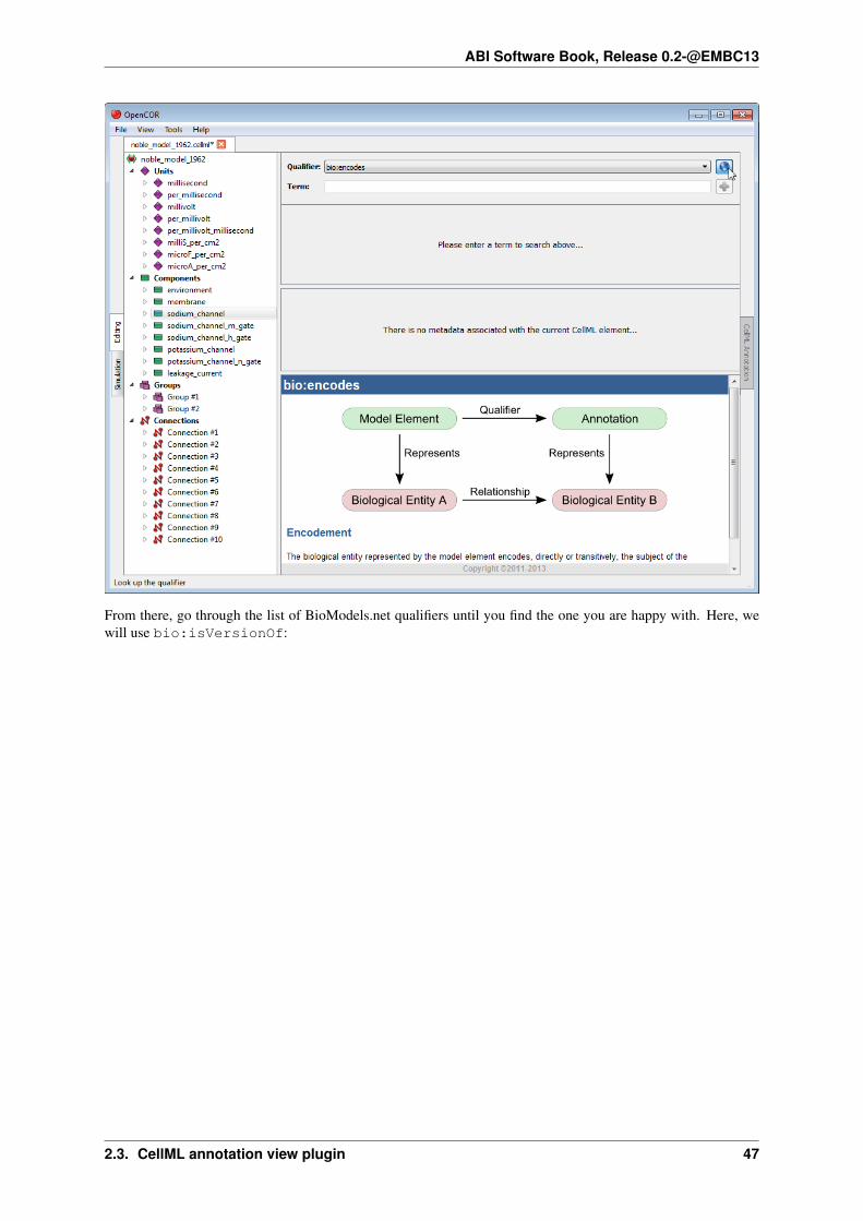
Next, you need to specify a BioModels.net qualifier. If you do not know which one to use, click on the
button to get some information about the current BioModels.net qualifier:
46 Chapter 2. OpenCOR
ABI Software Book, Release 0.2-@EMBC13
From there, go through the list of BioModels.net qualifiers until you find the one you are happy with. Here, wewill use bio:isVersionOf:
2.3. CellML annotation view plugin 47

ABI Software Book, Release 0.2-@EMBC13
Now, we need to retrieve some possible ontological terms to describe our sodium_channel component. Forthis, we must enter a search term which in our case is going to be sodium. OpenCOR is then going to use theRESTful service from SemanticSBML to provide us with a list of, here, 25 possible ontological terms:
48 Chapter 2. OpenCOR

ABI Software Book, Release 0.2-@EMBC13
A quick look through the list tells us that we probably want to use the ChEBI term which identifier is 29101. Ifyou want to know more about the ChEBI resource, you can click on its corresponding link:
2.3. CellML annotation view plugin 49

ABI Software Book, Release 0.2-@EMBC13
Similarly, if you want to know more about the ChEBI identifier:
50 Chapter 2. OpenCOR

ABI Software Book, Release 0.2-@EMBC13
Now that you are happy with your choice of ontological term, you can associate it with the sodium_channel
component by clicking on its corresponding button:
2.3. CellML annotation view plugin 51

ABI Software Book, Release 0.2-@EMBC13
As you will have seen, the ontological term you have just added cannot be added anymore, but it can be removedby clicking on its corresponding button or by using the context menu (see above).
Now, say that you also want to add the next ontological term. You can obviously do so by clicking on the
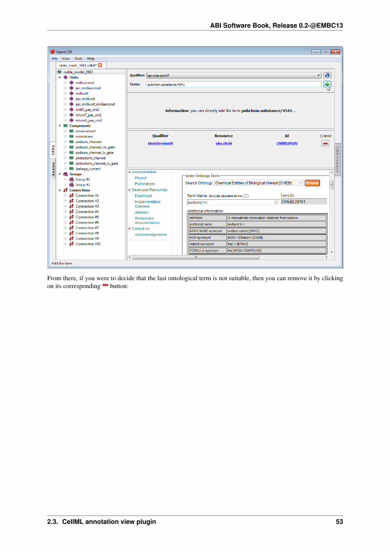
corresponding button, but you could also enter pubchem.substance/4541 (i.e.<resource>/<id>) in the term field. Indeed, OpenCOR will recognise this ‘term’ as being a valid ontologicalterm and will offer you to add it directly:
52 Chapter 2. OpenCOR
ABI Software Book, Release 0.2-@EMBC13
From there, if you were to decide that the last ontological term is not suitable, then you can remove it by clickingon its corresponding button:
2.3. CellML annotation view plugin 53

ABI Software Book, Release 0.2-@EMBC13
2.3.2 Unrecognised annotations
Annotations consist of RDF triples which are made of a subject, a predicate and an object. OpenCOR recognisesRDF triples which subject identifies a CellML element while it expects the predicate to be a BioModels.netqualifier and the object an ontological term.
Ontological terms used to be identified using MIRIAM URNs, but these have now been deprecated in favour ofidentifiers.org URIs. OpenCOR recognises both, but it will only serialise annotations using identifiers.org URIs.
Now, it may happen that a file contains annotations which do not fit OpenCOR’s current requirements. In thiscase, OpenCOR will display the annotations as a simple list of RDF triples:
54 Chapter 2. OpenCOR

ABI Software Book, Release 0.2-@EMBC13
If you ever come across a type of annotations which you think OpenCOR ought to recognise, but does not, thenplease do contact us.
2.4 CellML model repository plugin
The CellMLModelRepository plugin offers an interface to the CellML Model Repository. By default, it lists allthe CellML models found in the repository:
2.4. CellML model repository plugin 55
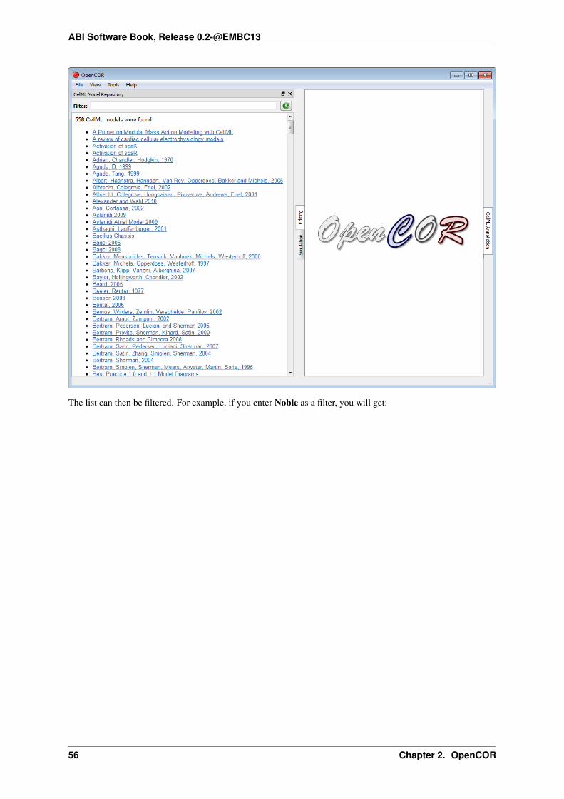
ABI Software Book, Release 0.2-@EMBC13
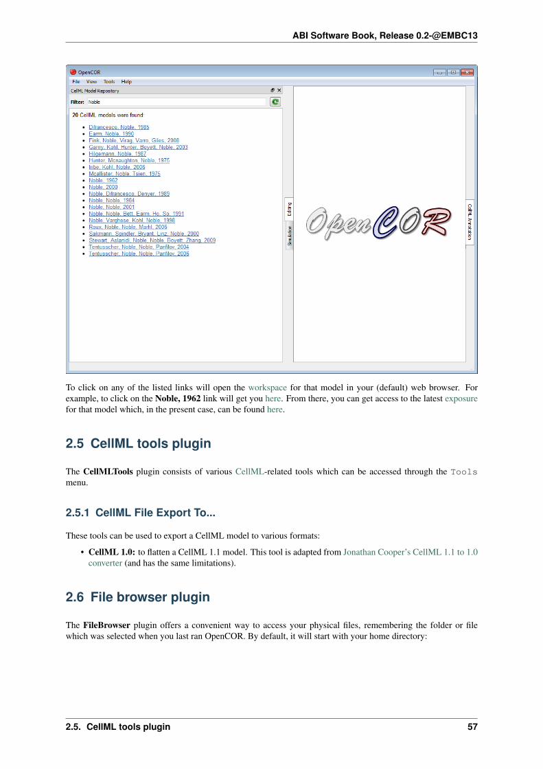
The list can then be filtered. For example, if you enter Noble as a filter, you will get:
56 Chapter 2. OpenCOR
ABI Software Book, Release 0.2-@EMBC13
To click on any of the listed links will open the workspace for that model in your (default) web browser. Forexample, to click on the Noble, 1962 link will get you here. From there, you can get access to the latest exposurefor that model which, in the present case, can be found here.
2.5 CellML tools plugin
The CellMLTools plugin consists of various CellML-related tools which can be accessed through the Toolsmenu.
2.5.1 CellML File Export To...
These tools can be used to export a CellML model to various formats:
• CellML 1.0: to flatten a CellML 1.1 model. This tool is adapted from Jonathan Cooper’s CellML 1.1 to 1.0converter (and has the same limitations).
2.6 File browser plugin
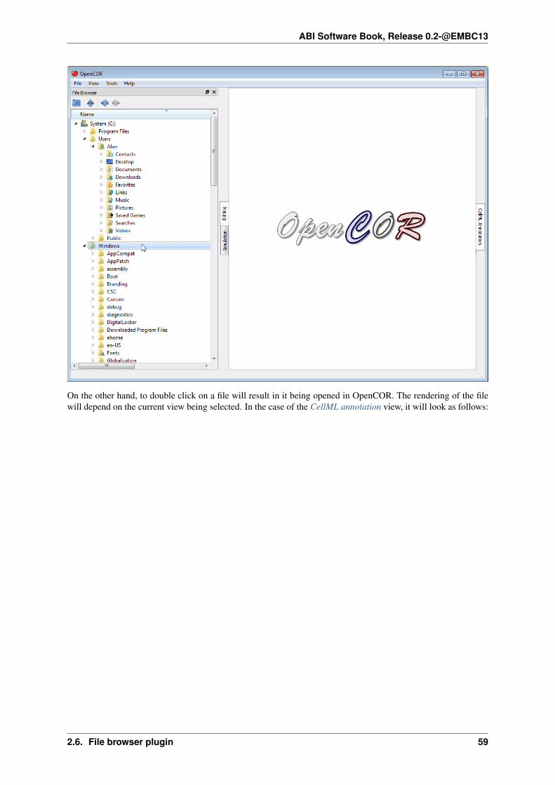
The FileBrowser plugin offers a convenient way to access your physical files, remembering the folder or filewhich was selected when you last ran OpenCOR. By default, it will start with your home directory:
2.5. CellML tools plugin 57

ABI Software Book, Release 0.2-@EMBC13
As you would expect, to double click on a folder will expand its contents, as can be seen by double clicking onthe Windows directory:
58 Chapter 2. OpenCOR
ABI Software Book, Release 0.2-@EMBC13
On the other hand, to double click on a file will result in it being opened in OpenCOR. The rendering of the filewill depend on the current view being selected. In the case of the CellML annotation view, it will look as follows:
2.6. File browser plugin 59

ABI Software Book, Release 0.2-@EMBC13
Folders and files can also be dragged from the File Browser window and dropped onto the file organiser window.
2.6.1 Tool bar
Go to the home folder
Go to the parent folder
Go to the previous folder or file
Go to the next folder or file
2.7 File organiser plugin
The FileOrganiser plugin allows you to organise your files virtually, i.e. independently of where they are physi-cally located. Your virtual environment is remembered from one session to another and is, by default, empty:
60 Chapter 2. OpenCOR

ABI Software Book, Release 0.2-@EMBC13
Now, say that you are working on a specific project. You might then want to create a (virtual) folder which contains
(a reference to) all the files you need for your project. To go about this, you first need to click on the buttonin the toolbar (or use the context menu). This will add a folder to your virtual environment:
2.7. File organiser plugin 61

ABI Software Book, Release 0.2-@EMBC13
You can rename the folder as you wish and create other (sub-)folders, if needed:
62 Chapter 2. OpenCOR

ABI Software Book, Release 0.2-@EMBC13
You can move the (sub-)folders around by dragging and dropping them within your virtual environment, or delete
an existing (sub-)folder by clicking on the button in the toolbar (or by using the contextmenu):
2.7. File organiser plugin 63

ABI Software Book, Release 0.2-@EMBC13
Next, you might want to open the file browser window, so you can start dragging and dropping files into yourvirtual environment (alternatively, you can use your system’s file manager):
64 Chapter 2. OpenCOR

ABI Software Book, Release 0.2-@EMBC13
As for folders, you can move and delete your (virtual) files:
2.7. File organiser plugin 65

ABI Software Book, Release 0.2-@EMBC13
2.7.1 Tool bar
Create a new folder
Delete the current folder(s) and/or link(s) to the current file(s)
2.8 Help plugin
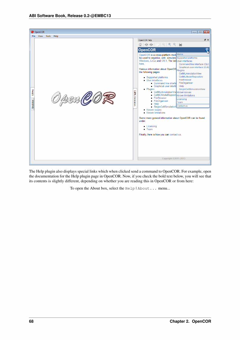
The Help plugin provides some user documentation which looks as follows:
66 Chapter 2. OpenCOR

ABI Software Book, Release 0.2-@EMBC13
The documentation includes a menu which gets shown whenever you move your mouse pointer over the informa-tion icon (top right):
2.8. Help plugin 67
ABI Software Book, Release 0.2-@EMBC13
The Help plugin also displays special links which when clicked send a command to OpenCOR. For example, openthe documentation for the Help plugin page in OpenCOR. Now, if you check the bold text below, you will see thatits contents is slightly different, depending on whether you are reading this in OpenCOR or from here:
To open the About box, select the Help | About... menu...
68 Chapter 2. OpenCOR

ABI Software Book, Release 0.2-@EMBC13
2.8.1 Tool bar
Go to the home page
Go back
Go forward
Copy the selection to the clipboard
Reset the size of the help page contents
Zoom in the help page contents
Zoom out the help page contents
Print the help page contents
2.9 Single cell view plugin
The SingleCellView plugin can be used to run CellML models which consists of either a system of ordinarydifferential equations (ODEs) or differential algebraic equations (DAEs). The system may be non-linear.
2.9.1 Open a CellML file
Upon opening a CellML file, OpenCOR will check that it can be used for simulation. If it cannot, then a messagewill describe the issue:
2.9. Single cell view plugin 69

ABI Software Book, Release 0.2-@EMBC13
Alternatively, if the CellML file is valid, then the view will look as follows:
70 Chapter 2. OpenCOR

ABI Software Book, Release 0.2-@EMBC13
The view consists of two main parts, the first of which allows you to customise the simulation, the solver andthe model parameters. The second part is used to plot simulation data. In the parameters section, each modelparameter has an icon associated with it to highlight its type:
(Editable) constant
Computed constant
(Editable) state
Rate
Algebraic
2.9. Single cell view plugin 71

ABI Software Book, Release 0.2-@EMBC13
2.9.2 Simulate an ODE model
To simulate a model, you need to provide some information about the simulation itself, i.e. its starting point,ending point and point interval. Then, you need to specify the solver that you want to use. The solvers availableto you will depend on which solver plugins you selected, as well as on the type of your model (i.e. ODE or DAE).In the present case, we are dealing with an ODE model and all the solver plugins are selected, so OpenCOR offersCVODE, forward Euler, Heun, Midpoint, and second- and fourth-order Runge-Kutta as possible solvers for ourmodel.
Each solver comes with its own set of properties which you can customise. For example, if we select Euler(forward) as our solver, then we can customise its Step property:
72 Chapter 2. OpenCOR
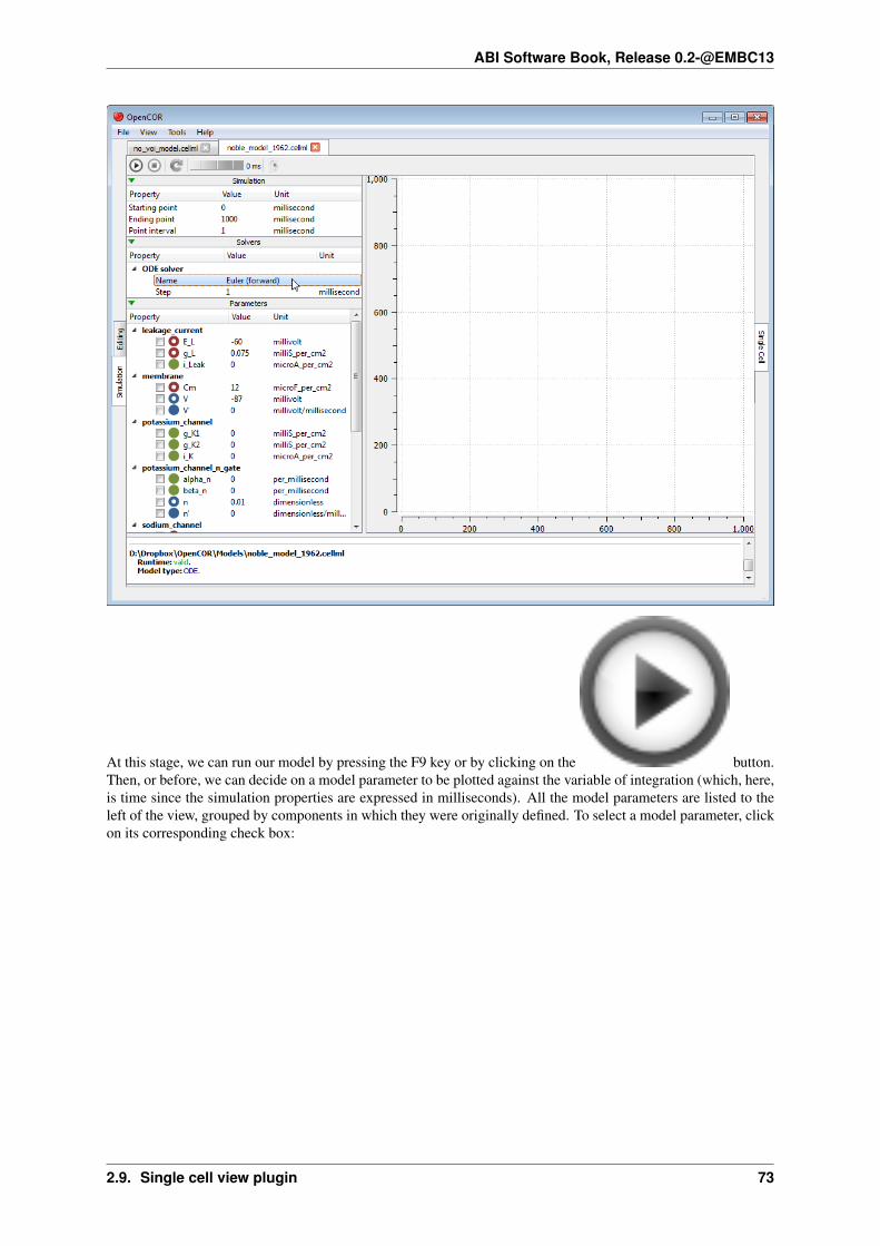
ABI Software Book, Release 0.2-@EMBC13
At this stage, we can run our model by pressing the F9 key or by clicking on the button.Then, or before, we can decide on a model parameter to be plotted against the variable of integration (which, here,is time since the simulation properties are expressed in milliseconds). All the model parameters are listed to theleft of the view, grouped by components in which they were originally defined. To select a model parameter, clickon its corresponding check box:
2.9. Single cell view plugin 73

ABI Software Book, Release 0.2-@EMBC13
As can be seen, the simulation failed. Several model parameters, including the one we selected, have a nan value(i.e. not a number). In this case, it is because the solver was not properly set up. Its Step property is too big.
If we set it to 0.01 milliseconds, reset the model parameters (by clicking on thebutton), and restart the simulation, then we get the following trace:
74 Chapter 2. OpenCOR

ABI Software Book, Release 0.2-@EMBC13
The (roughly) same trace can also be obtained using CVODE as our solver:
2.9. Single cell view plugin 75

ABI Software Book, Release 0.2-@EMBC13
However, the simulation is so quick to run that we do not get a chance to see the progress of the simulation.
Between the and buttons, there is a wheel which we can use to add a short delaybetween the output of two data points. Here, we set the delay to 13 ms. This allows us to rerun the simulation,after having reset the model parameters, and pause it at a point of interest:
76 Chapter 2. OpenCOR

ABI Software Book, Release 0.2-@EMBC13
Now, we can modify any of the model parameters identified by either the or icon,but let us just modify g_Na_max (under the sodium_channel component) by setting its value to 0milliS_per_cm2. Then, we resume the simulation and we can see the effect on the model:
2.9. Single cell view plugin 77

ABI Software Book, Release 0.2-@EMBC13
If we want, we could export all the simulation data to a comma-separated values (CSV) file. To do so, we need to
click on the button.
2.9.3 Simulate a DAE model
To simulate a DAE model is similar to simulating an ODE model, except that OpenCOR only offers one DAEsolver (IDA) at this stage:
78 Chapter 2. OpenCOR

ABI Software Book, Release 0.2-@EMBC13
2.9.4 Simulate a CellML 1.1 model
So far, we have only simulated CellML 1.0 models, but we can also simulate CellML 1.1 models, i.e. modelswhich import units and/or components from other models:
2.9. Single cell view plugin 79

ABI Software Book, Release 0.2-@EMBC13
2.9.5 Simulate several models at the same time
Each simulation is run in its own thread which means that several simulations can be run at the same time.Simulations running in the ‘background’ display a small progress bar in the top tab bar while the ‘foreground’simulation uses the main progress bar at the bottom of the view:
80 Chapter 2. OpenCOR

ABI Software Book, Release 0.2-@EMBC13
2.9.6 Plotting area
The plotting area offers several features which can be activated by:
• Zooming in:
– holding the right mouse button down, and moving the mouse to the right/bottom to zoom in onthe X/Y axis; or
– moving the mouse wheel up.
• Zooming out:
– holding the right mouse button down, and moving the mouse to the left/top to zoom out on theX/Y axis; or
– moving the mouse wheel down.
• Zooming into a region of interest:
– pressing Ctrl and holding the right mouse button down, and moving the mouse around.
• Panning:
– holding the left mouse button down, and moving the mouse around (this obviously requires theplotting area to having been zoomed in in the first place).
• Coordinates of any point:
– pressing Shift and holding the left mouse button down, and moving the mouse around.
• Copying the contents of the plotting area to the clipboard:
– double-clicking the left mouse button.
2.9. Single cell view plugin 81

ABI Software Book, Release 0.2-@EMBC13
2.9.7 Tool bar
Run the simulation
Pause the simulation
Stop the simulation
Reset all the model parameters
Export the simulation data to CSV
2.10 Supported platforms
OpenCOR can be used on the following versions of Windows, Linux and OS X.
2.10.1 Windows
OpenCOR is supported on the 32-bit and 64-bit versions of Windows XP, Windows Vista, Windows 7 and Win-dows 8.
2.10.2 Linux
OpenCOR is supported on the 32-bit and 64-bit versions of Ubuntu 12.04 LTS (Precise Pangolin), 12.10 (QuantalQuetzal) and 13.04 (Raring Ringtail), but it might also work with earlier versions of Ubuntu, as well as some otherLinux distributions, though additional system libraries might be needed for the latter.
82 Chapter 2. OpenCOR
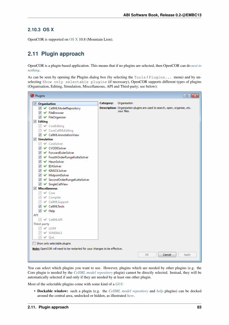
ABI Software Book, Release 0.2-@EMBC13
2.10.3 OS X
OpenCOR is supported on OS X 10.8 (Mountain Lion).
2.11 Plugin approach
OpenCOR is a plugin-based application. This means that if no plugins are selected, then OpenCOR can do next tonothing.
As can be seen by opening the Plugins dialog box (by selecting the Tools | Plugins... menu) and by un-selecting Show only selectable plugins (if necessary), OpenCOR supports different types of plugins(Organisation, Editing, Simulation, Miscellaneous, API and Third-party; see below):
You can select which plugins you want to use. However, plugins which are needed by other plugins (e.g. theCore plugin is needed by the CellML model repository plugin) cannot be directly selected. Instead, they will beautomatically selected if and only if they are needed by at least one other plugin.
Most of the selectable plugins come with some kind of a GUI:
• Dockable window: such a plugin (e.g. the CellML model repository and help plugins) can be dockedaround the central area, undocked or hidden, as illustrated here.
2.11. Plugin approach 83

ABI Software Book, Release 0.2-@EMBC13
• View window: such a plugin (e.g. the CellML annotation view and single cell view plugins) is used tointeract with a file, be it to edit it, simulate it or analyse it.
2.11.1 Organisation
Organisation plugins are used to search, open, organise, etc. your files:
• CellMLModelRepository: a plugin to access the CellML model repository.
• FileBrowser: a plugin to access your local files.
• FileOrganiser: a plugin to virtually organise your files.
2.11.2 Editing
Editing plugins are used to edit part or all of your files using one of several possible views:
• CellMLAnnotationView: a plugin to annotate CellML files.
There are also some non-selectable Editing plugins:
• CoreEditing: the core editing plugin.
• CoreCellMLEditing: the core CellML editing plugin.
2.11.3 Simulation
Simulation plugins are used to simulate your files:
• CVODESolver: a plugin which uses CVODE to solve ODEs.
• ForwardEulerSolver: a plugin which implements the Forward Euler method to solve ODEs.
• FourthOrderRungeKuttaSolver: a plugin which implements the fourth-order Runge-Kutta method tosolve ODEs.
• HeunSolver: a plugin which implements the Heun method to solve ODEs.
• MidpointSolver: a plugin which implements the Midpoint method to solve ODEs.
• IDASolver: a plugin which uses IDA to solve DAEs.
• KINSOLSolver: a plugin which uses KINSOL to solve non-linear algebraic systems.
• SecondOrderRungeKuttaSolver: a plugin which implements the second-order Runge-Kutta method tosolve ODEs.
• SingleCellView: a plugin to run single cell simulations.
There is also a non-selectable Simulation plugin:
• CoreSolver: the core solver plugin.
2.11.4 Miscellaneous
Miscellaneous plugins are used for various purposes:
• Help: a plugin to provide help.
There are also some non-selectable Miscellaneous plugins:
• Core: the core plugin.
• Compiler: a plugin to support code compilation.
• CellMLSupport: a plugin to support CellML.
84 Chapter 2. OpenCOR

ABI Software Book, Release 0.2-@EMBC13
• CellMLTools: a plugin to access various CellML-related tools.
2.11.5 API
(Non-selectable) API plugins are used to provide access to external APIs:
• CellMLAPI: a plugin to access the CellML API.
2.11.6 Third-party
(Non-selectable) third-party plugins are used to provide access to third-party libraries:
• LLVM: a plugin to access LLVM (as well as Clang).
• SUNDIALS: a plugin to access CVODE, IDA and KINSOL from the SUNDIALS library.
• Qwt: a plugin to access Qwt.
2.11. Plugin approach 85

ABI Software Book, Release 0.2-@EMBC13
86 Chapter 2. OpenCOR

CHAPTER 3
MAP Client
The MAP Client is a cross-platform framework for managing workflows. MAP Client is a plugin-based applicationthat can be used to create workflows from a collection of workflow steps.
The MAP Client is an application written in Python and based on Qt the cross-platform application and UI frame-work. Further details are available in the documents listed below.
3.1 MAP Installation and Setup Guide
This document describes how to install and setup the MAP software for use on your machine. The MAP softwareis a Python application that uses the PySide Qt library bindings. The instructions in this document cover theinstallation and setup on a Windows based operating system. The instructions for GNU/Linux and OS X aresimilar and should be extrapolated from these instructions. There are some side notes for these other operatingsystems to help, but not full or dedicated instructions. If for any reason you get stuck and cannot complete theinstructions please contact us.
3.1.1 MAP
The MAP framework is written in Python and is designed to work with Python 2 and Python 3. The MAP appli-cation is tested against Python2.6, Python2.7 and Python3.3 and should work with any of these Python libraries.Currently the MAP framework is not packaged as an application, requiring the user to set up the environment priorto launching the mapclient.py executable Python script.
The MAP application consists of the framework and various tools, by itself it can do very little. It is the job ofthe plugins to provide functionality. The MAP application as referred to in this section of the instructions may bedescribed as the barebones application for this reason.
To execute the barebones application we need to first install some dependencies:
1. Python (and make sure to add the Python and Python\Scripts folders to your systemPATH).
2. PySide (PySide and PyQt4 are virtually interchangeable but currently this would require sometextual changes)
3. Python setup tools and then using easy_install.exe to install:
1. Requests Python library (easy_install requests)
2. OAuthlib Python library (not the OAuth Python library) (easy_install oauthlib).
Also, if we wish to interact with the Physiome Model Repository (PMR) we need:
1. Mercurial
We can now install the barebones MAP client application. The barebones application can be launched via thecommand window with the following command in the extracted mapclient/src folder:
87
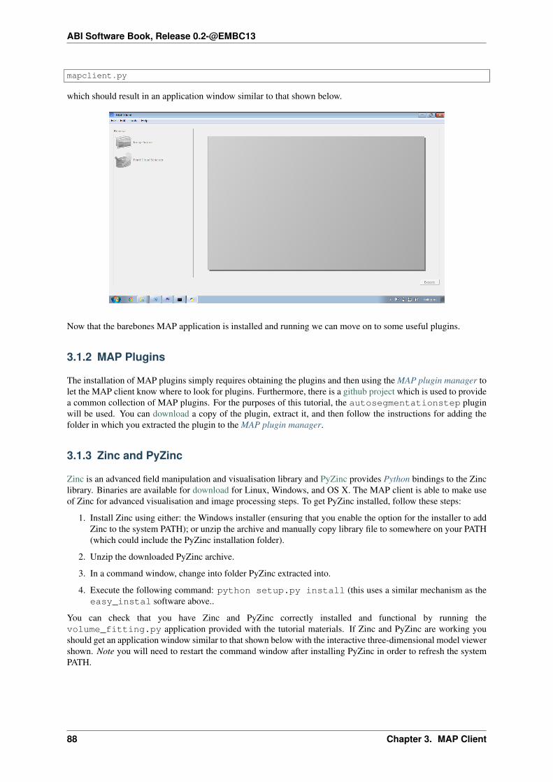
ABI Software Book, Release 0.2-@EMBC13
mapclient.py
which should result in an application window similar to that shown below.
Now that the barebones MAP application is installed and running we can move on to some useful plugins.
3.1.2 MAP Plugins
The installation of MAP plugins simply requires obtaining the plugins and then using the MAP plugin manager tolet the MAP client know where to look for plugins. Furthermore, there is a github project which is used to providea common collection of MAP plugins. For the purposes of this tutorial, the autosegmentationstep pluginwill be used. You can download a copy of the plugin, extract it, and then follow the instructions for adding thefolder in which you extracted the plugin to the MAP plugin manager.
3.1.3 Zinc and PyZinc
Zinc is an advanced field manipulation and visualisation library and PyZinc provides Python bindings to the Zinclibrary. Binaries are available for download for Linux, Windows, and OS X. The MAP client is able to make useof Zinc for advanced visualisation and image processing steps. To get PyZinc installed, follow these steps:
1. Install Zinc using either: the Windows installer (ensuring that you enable the option for the installer to addZinc to the system PATH); or unzip the archive and manually copy library file to somewhere on your PATH(which could include the PyZinc installation folder).
2. Unzip the downloaded PyZinc archive.
3. In a command window, change into folder PyZinc extracted into.
4. Execute the following command: python setup.py install (this uses a similar mechanism as theeasy_instal software above..
You can check that you have Zinc and PyZinc correctly installed and functional by running thevolume_fitting.py application provided with the tutorial materials. If Zinc and PyZinc are working youshould get an application window similar to that shown below with the interactive three-dimensional model viewershown. Note you will need to restart the command window after installing PyZinc in order to refresh the systemPATH.
88 Chapter 3. MAP Client

ABI Software Book, Release 0.2-@EMBC13
Which Binary?
There are a number of binaries available for any given platform and you must match the package description withyour system setup. The package description contains the package name, package version, package architecture,package operating system and in the case of PyZinc the package Python version. The package extension indicatesthe type of package and they come in two main flavours: installer/package manager; archive.
Additionally the version of the PyZinc binaries you download must match the version of the Zinc library binaries.
3.2 MAP Features Demonstration
Section author: Hugh Sorby
Note: MAP is currently under active development, and this document will be updated to reflect any changes tothe software or new features that are added. You can follow the development of MAP at the launchpad project.
This document details the features of MAP, a cross-platform framework for managing workflows. MAP is aplugin-based application that can be used to create workflows from a collection of workflow steps.
In this demonstration is based on version 0.9.0 of MAP, available from the project downloads. Directions forinstalling MAP and getting the MAP plugins are available in the MAP Installation and Setup Guide.
In this demonstration we will cover the features of MAP. We will start with a quick tour and then create a newworkflow that will help us segment a region of interest from a stack of images.
3.2.1 Quick Tour
When you first load MAP, it will look something like this:
In the main window we can see three distinct areas that make up the workflow management side of the software.These three areas are the menu bar (at the top), the step box (on the left) that contains the steps that you can use tocreate your workflow and the workflow canvas (on the right) an area for constructing a workflow.
3.2. MAP Features Demonstration 89

ABI Software Book, Release 0.2-@EMBC13
In the Step box we will only see two steps, this is because we have only loaded the default Steps and not loadedany of the external plugins that MAP can use.
Menu Bar
The Menu bar provides a selection of drop down menus for accessing the applications functions. The File menuprovides access to opening, importing, closing workspaces as well as quitting the application. The Edit menuprovides access to the undo/redo functionality. The Tools menu provides access to the Plugin Manager tool,Physiome Model Repository (PMR) tool and the Annotation tool. The Help menu provides access to the aboutbox which contains information on contributors and the license that the MAP application is released under.
Step Box
The Step box provides a selection of steps that are available to construct a workflow from. The first time we startthe program only the default plugins are available. To add more steps we can use the Plugin Manager tool. To usea step in our workflow we drag the desired step from the step box onto the workflow canvas.
Workflow canvas
The workflow canvas is where we construct our workflow. We do this by adding the steps to the workflow canvasfrom the step box that make up our workflow. We then make connections between the workflow steps to definethe complete workflow.
When a step is added to the workflow the icon which is visible in the Step box is augmented with visualisationsof the Steps ports and the steps configured status. The annotation of the steps ports will show when the mouse ishovered over a port. The image below shows the Image Source step with the annotation for the port displayed.
3.2.2 Tools
MAP currently has three tools that may be used to aide the management of the workflow. They are the PluginManager tool, the Physiome Model Repository (PMR) tool and the Annotation tool. For a description of each toolsee the relevant sections.
90 Chapter 3. MAP Client

ABI Software Book, Release 0.2-@EMBC13
Plugin Manager Tool
The plugin tool is a simple tool that enables the user to add or remove additional plugin directories. MAP comeswith some default plugins which the user can decide to load or not. External directories are added with the adddirectory button. Directories are removed by selecting the required directory in the Plugin directories list andclicking the remove directory button.
Whilst additions to the plugin path will be visible immediately in the Step box deletions will not be apparent untilthe next time the MAP Client is started. This behaviour is a side-effect of the Python programming language.
Physiome Model Repository (PMR) Tool
The PMR tool uses webservices and OAuth to communicate between itself (the consumer) and the PMR website(the server). Using this tool we can search for and find suitable resources on PMR.
The PMR website uses OAuth to authenticate a consumer and determine consumer access privileges. Here wewill discuss the parts of OAuth that are relevant to getting you (the user) able to access resources on PMR.
In OAuth we have three players the server, the consumer and the user. The server is providing a service that theconsumer wishes to use. It is up to the user to allow the consumer access to the servers resources and set the levelof access to the resource. For the the consumer to access privileged information of the user stored on the serverthe user must register the consumer with the server, this is done by the user giving the consumer a temporaryaccess token. This temporary access token is then used by the consumer to finalise the transaction and acquirea permanent access token. The user can deny the consumer access at anytime by logging into the server andrevoking the permanent access token.
If you want the PMR tool to have access to privileged information (your non-public workspaces stored on PMR)you will need to register the PMR tool with the PMR website. We do this by clicking on the register link as shownin the figure below. This does two things: it shows the Application Authorisation dialog; opens a webbrowserat the PMR website. [If you are not logged on at the PMR website you will need to do so now to continue,instructions on obtaining a PMR account are availble here]. On the PMR website you are asked to either accept ordeny access to the PMR tool. If you allow access then the website will display a temporary access token that youwill need to copy and paste into the Application Authorisation dialog so that the PMR tool can get the permanentaccess token.
Annotation Tool
The Annotation tool is a very simple tool to help a user annotate the Workflow itself and the Step data directoriesthat are linked to PMR. At this stage there is a limited vocabulary that the Annotation tool knows about, but thisis intended to be extended in coming releases. The vocabulary that the annotation is aware of is available in thethree combo-boxes near the top of the dialog.
The main part of the Annotation tool shows the current annotation from the current target.
In the above image we can see the list of annotations that have been added to the current target. This is a simplifiedview of the annotation with the prefix of the terms removed for clarity.
3.2. MAP Features Demonstration 91

ABI Software Book, Release 0.2-@EMBC13
3.3 MAP Tutorial - Create Workflow
Section author: Hugh Sorby
Note: MAP is currently under active development, and this document will be updated to reflect any changes tothe software or new features that are added. You can follow the development of MAP at the launchpad project.
This document details takes the reader through the process of creating a workflow from existing MAP plugins.Having a read through the MAP Features Demonstration is a good way to become familiar with the features of theMAP application.
3.3.1 Getting Started
To get started with MAP we need to create a new workflow. To do this we use File → New → Workflow menuoption (Ctrl-N shortcut). This option will present the user with a directory selection dialog. Use the dialog toselect a directory where the workflow can be saved. Once we have chosen a directory the step box and workflowcanvas will become enabled.
To create a meaningful workflow we will need to use some external plugins. To load these plugins we will use thePlugin Manager tool. The Plugin Manager tool can be found under the Tools menu. Use the Plugin Manager toadd the directory location of the MAP Plugins. After confirming the changes to the Plugin Manager you shouldsee a few new additions to the Step box.
92 Chapter 3. MAP Client

ABI Software Book, Release 0.2-@EMBC13
3.3.2 Creating the Workflow
To create a workflow we use Drag ‘n’ Drop to drag steps from the Step box and drop the step onto the workflowcanvas. When steps are first dropped onto the canvas they show a red cog icon to indicate that the step is notconfigured. At a minimum a step requires an identifier to be set before it can be used.
Drag the steps Image Source, Data Store and Automatic Segmenter onto the workflow canvas. All the steps willshow a red cog, except the ‘Automatic Segmenter’, step this indicates that the step needs to be configured. Toconfigure a step we can either right click on the step to bring up a context menu from which the configure actioncan be chosen or simply click the red cog directly. See the relevant section for the configuration of a particularstep.
Note: When configuring a step you are asked to set an identifier. The identifier you set must unique within theworkflow and it must not start with a ‘.’.
Configuring the Image Source Step
The Image Source step requires a location. This location contains the images to import. The location may be adirectory on the local hard disk or a workspace on PMR. Here we will show how to configure the Image Sourcestep with images that have been stored in a workspace on PMR.
First each step requires a unique id. The id is used to create a file containing the step configuration information.This id for the Image Source step is used to create a directory under the workflow project directory. In the identifieredit box enter a directory name. Once a valid identifier is entered the red highlight around the edit box will beturned off.
Next change to the PMR tab and we will see an ellipses button for bringing up the PMR tool dialog. You need toregister the PMR tool to access certain webservices the details on how to do this are available here. The remainderof this tutorial will assume you have setup access to PMR properly. In the search box of the PMR dialog we needto enter the search term ‘blood-vessels’. The result of the search should look like the image below.
Select this entry in the search listing and click ‘Ok’. The selected PMR workspace will be downloaded in thebackground. When the download is finished the red cog icon will disappear. If the download is not successful adialog will appear to inform you of the error.
MAP is not setup to work with streamed resources so we must download the workspace from PMR.
3.3. MAP Tutorial - Create Workflow 93

ABI Software Book, Release 0.2-@EMBC13
Configuring the Point Cloud Step
Configuring the Point Cloud step is trivial at this time. This is because the step only requires an identifier to beset. The identifier will be used to create a directory where the received point cloud will be serialized.
3.3.3 Executing the Workflow
At this point you should have a workflow area looking like this:
Once the All the steps in the workflow are configured (no more red cog icons) we can make connections betweenthe steps. To make a connection between two steps the first step must provide what the second step uses. Whentrying to connect two steps that cannot be connected you will see a no entry icon over the connection for a shortperiod of time and then the connection will be removed. The following image shows an incorrect connectiontrying to be made.
If the mouse is hovered over a port you will see a description of what the port provides or uses. To make aconnection click on a port and drag the mouse to the port to be connected.
To execute the workflow we need to connect up the steps in the correct manner and save the workflow. Theworkflow should be connected up as can be seen in the following image.
Once the workflow has been saved the execute button in the lower left corner should become enabled. Clickingthe execute button will, naturally enough, execute the workflow step by step.
Note: We can make connections between steps at anytime not just when all steps have been properly configured.
94 Chapter 3. MAP Client

ABI Software Book, Release 0.2-@EMBC13
Automatic Segmenter Step
The ‘Automatic Segmenter’ actually allows us to interact with executing workflow. With this step we can movethe image plane up and down and change the visibility of the graphical items in the scene. The image plane ismoved through the use of the slider on the left hand side. The visibility of the graphical items is controlled bychecking or unchecking the relevant check boxes.
3.4 MAP Plugins
The Plugin lies at the heart of the MAP framework. The key idea behind the plugins is to make them as simple aspossible to implement. The interface is defined in documentation and the plugin developer is expected to adhereto it. The framework leaves the responsibility of conforming to the plugin interface up to the plugin developer.The plugin framework is based on Marty Alchin’s [1] article on a plugin framework for Django. The pluginframework is very lightweight and requires no external libraries and can be made to work with Python 2 andPython 3 simultaneously.
3.4.1 Workflow Step
The Workflow Step is the basic item that a plugin developers need to place their software within. A workflowstep can be of any size and complexity. Although it must adhere to the plugin design to work properly withthe application. Every step that wishes to act like a Workflow Step must derive itself from the Workflow stepmountpoint. The Workflow step mountpoint is the interface between the application and the plugin. The Workflowstep mountpoint can be imported like so:
from mountpoints.workflowstep import WorkflowStepMountPoint
A skeleton step is provided as a starting point for the developer to create their own workflow steps. The skeletonstep is actually a valid step in its own right and it will show up in the Step box if enabled. However the skeletonstep has no use other than as an item to drag around on the workflow area. The skeleton step is discussed below,first however the plugin interface is discussed.
Plugin Interface
The plugin interface is the layer between the application and the developers plugin. The plugin interface is notdefined by contract as we so often see in Java. But rather the plugin interface is defined by documentation. Thisputs the burden of the specification on the documentation and the conformity of the specification on the developer.
3.4. MAP Plugins 95

ABI Software Book, Release 0.2-@EMBC13
The underlying theory is that the developer is able to follow the specification without the application having to dorigourous checks to make sure this is the case. The phrase ‘If it walks like a duck’ is often used.
In this section the specification of the Workflow step plugin interface is given. It is then upto the developer tomake sure their plugin behaves like one.
The details of the plugin interface are provided in the documentation of the source code in the relevant sourcefile and additionally here for easy reference. The documentation provided with the source code is very directwith little explanation the following documentation provides a bit more explanation and discussion on the variousaspects of the plugin interface. The documentation provided here should be considered the slave documentationand the documentation provided with the source code as the master documentation.
There are essentially, what may be considered, three different levels of the plugin design.
1. The Musts
2. The Shoulds
3. The Coulds
Creating a workflow step that satisifies the musts will create an actual workflow step that can be added to theworkflow area and interacted with. But it won’t be very useful. Satisfying the shoulds will usually be sufficientfor the very simplest of steps. Simple steps are for instance ones that provide images, or location information fordata. Doing some of the coulds will create a much more interesting step.
The requirements for creating a step have been kept as simple as possible, this is to allow the developer a quickroute into the development of the step content.
The following three sections discuss these three levels in more detail.
A Step Must
• The plugin must be derived from the WorkflowStepMountPoint class defined in the package mount-points.workflowstep
• Accept a single parameter in it’s __init__ method.
• Define a name for itself, this must be passed into the initialisation of the base class.
• Define the methods
def configure(self):pass
def getIdentifier(self):pass
def setIdentifier(self, identifier):pass
def serialize(self, location):pass
def deserialize(self, location):pass
A Step Should
• Implement the configure method to configure the step. This is typically in the form of a dialog. When imple-menting this function the class method self._configureObserver() should be called to inform the applicationthat the step configuration has finished.
• Implement the getIdentifier/setIdentifier methods to return the identifier of the step.
96 Chapter 3. MAP Client

ABI Software Book, Release 0.2-@EMBC13
• Implement the serialize/deserialize methods. The steps should serialize and deserialize from a file on disklocated at the given location.
• Define a class attribute _icon. That is of the type QtGui.QImage.
• Information about what the step uses and/or what it provides. This is achieved through defining ports on thestep.
A Step Could
• Implement the method ‘portOutput(self)’ if it was providing some information to another step.
• Implement the method ‘execute(self, dataIn)’ if it uses some information from another step. If a step imple-ments the ‘execute(self, dataIn)’ method then it must call ‘_doneExecution()’ when the step is finished.
• Define a category using the ‘_category’ attribute. This attribute will add the step to the named category inthe step box, or it will create the named category if it is not present.
3.4.2 Ports
A port is a device to specify what a workflow step provides or uses. A port is described using Resource DescriptionFramework (RDF) triples. The port description is used to determine whether or not two ports may be connectedtogether. One port can either use or provide one thing. A single port must not both provide a thing and use a thing.Ports are ordered by entry position.
Ports are added by using the ‘addPort(self, triple)’ method from the base class.
3.4.3 Skeleton Step
The skeleton step satisfies the musts of the plugin interface. It is a minimal step and it is set out as follows.
A Python package with the step name is created, in this case ‘skeletonstep’, in the module file we add the codethat needs to be read when the plugins are loaded.
The module file performs four functions. It contains the version information and the authors name of the module.For instance the skeleton step has a version of ‘0.1.0’ and authors name of ‘Xxxx Yyyyy’. It adds the currentdirectory into the Python path, this is done so that the steps python files know where they are in relation to thepython path. It also (optionally) prints out a message showing that the plugin has been loaded successfully. But themost important function it performs is to call the python file that contains the class that derives from the workflowstep mountpoint.
The ‘SkeletonStep’ class in the skeletonstep.step package is a very simple class. It derives from the ‘Workflow-StepMountPoint’, calls the base class with the name of the step, accepts a single parameter in it’s init method anddefines the five required functions to satisfy the plugin interface.
When enabled the skeleton step will be a fully functioning step in the MAP Client.
3.4.4 References
[1] http://martyalchin.com/2008/jan/10/simple-plugin-framework/ Marty Alchin on January 10, 2008
3.5 MAP Tutorial - Create Plugin
Section author: Hugh Sorby
Note: MAP is currently under active development, and this document will be updated to reflect any changes tothe software or new features that are added. You can follow the development of MAP at the launchpad project.
3.5. MAP Tutorial - Create Plugin 97

ABI Software Book, Release 0.2-@EMBC13
This document details takes the reader through the process of creating a new plugin for the MAP Client. The MAPPlugins document defines the plugin interface that the new plugin must adhere to.
3.5.1 A Simple Source Step Example
We need to create a source step for supplying Zinc model files.
First copy the skeletonstep directory to another directory. To make this step our own we first change the skeleton-step name to zincmodelsourcestep. The places we have to change are:
1. The topmost directory
2. The inner directory, this directory is used to namespace our new step.
3. In __init__.py file in the topmost directory, we also need to uncomment the lines:
from zincmodelsourcestep import step print(“Plugin ‘{0}’ version {1} by {2} loaded”.format(tail, __ver-sion__, __author__))
4. In __init__.py file in the inner directory. We have to change the name of the class to ‘ZincModelSourceStep’and change the name of the step to ‘Zinc Model Source’.
Now we need to be able to configure the step. To do this we can use qt-designer to create a ‘configuredialog.ui’file that we can convert into Python code using ‘pyside-uic’.
98 Chapter 3. MAP Client

CHAPTER 4
Developing the Virtual Physiological Human
This tutorial will demonstrate tools, techniques and best practices that aid scientists in the development and ap-plication of computational models and simulation experiments in their work toward the creation of a virtual phys-iological human. The Physiome Model Repository (PMR) provides a framework for the storage, curation andexchange of data. By using standards suitable to their data, scientists maximise their ability to reuse existingknowledge and enable others to make use of their achievements in novel work. Annotations ensure scientists areable to find existing data and are also able to correctly interpret and apply their own data. These tutorials aredesigned to help demonstrate and promote practices which will aid attendees in their own work. Attendees areencouraged to raise issues specifically related to their needs with the tutors.
Documentation for the software used in this tutorial is available online, including the most recent version of thistutorial itself. This tutorial guides the particpant through three common computational modelling scenarios facedby scientists working toward the virtual physiologial human. We use these scenarios to achieve scientific outputsusing the covered tools tools and demonstrating practices we believe will help ensure reproducible and reusablescience. Each of the scenarios listed below should be worked through in order and in each scenario we provideexamples using either OpenCOR or the MAP workflow tool.
When interacting directly with Mercurial, this tutorial demonstrates how to work with the Physiome Model Repos-itory using TortoiseHg, which provides a Windows explorer integrated system for working with Mercurial reposi-tories.
Brief mention of the equivalent command line versions of the TortoiseHgactions will also be mentioned, so that these ideas can also be used withouta graphical client, and on Linux or OS X and similar systems. These will be denotedby boxes like this.
This tutorial requires you to have:
• A Mercurial client such as TortoiseHg or Mercurial installed;
• The OpenCOR CellML modelling environment and/or the MAP workflow tool installed; and
• A text editor such as Notepad++ or gedit.
4.1 Creating a new piece of work
In the Physiome Model Repository (PMR), a complete piece of work is stored in a workspace. Each workspaceis a Mercurial repository, which allows PMR to maintain a complete history of all changes made to every file itcontains. In this tutorial, we take you through the creation of a new piece of work which will be stored in a PMRworkspace:
4.1.1 Working with the repository using Mercurial
This part of the tutorial will teach you how to create a workspace in the repository, clone the workspace from themodel repository using a Mercurial client, add content to the workspace, and then push the cloned workspace to
99
ABI Software Book, Release 0.2-@EMBC13
the repository.
Registering an account and logging in
First, navigate to the teaching instance of the Physiome Model Repository at http://teaching.physiomeproject.org/.
Note: The teaching instance of the repository is a mirror of the main repository site found athttp://models.physiomeproject.org/, running the latest development version of the PMR Software.
Any changes you make to the contents of the teaching instance are not permanent, and will be overwritten withthe contents of the main repository whenever the teaching instance is upgraded to a new PMR Software release.For this reason, you can feel free to experiment and make mistakes when pushing to the teaching instance. Pleasesubscribe to the cellml-discussion mailing list to receive notifications of when the teaching instance will be re-freshed.
See the section Migrating content to the main repository for instructions on how to migrate any content from theteaching instance to the main (permanent) Physiome Model Repository.
In order to make changes to models in the repository, you must first register for an account. If you already havean account on the main repository site, your account will also be on the teaching instance. Otherwise, you need toregister for an account on the teaching repository. You can register by navigating to the Log in link at the top rightof the menu bar and then looking for the New user section of the log in page.
Note: Your username and password are also the credentials you use to interact with the repository via Mercurial.
Once logged in to the repository, you will notice that there are a couple of new links in the navigation bar (MyWorkspaces and Documentation). The My Worskpaces link is where all the workspaces you create later on will belisted. The Log in link is also replaced by your username and a Log out link (which you can access by clicking onyour username).
Mercurial username configuration
Important: Username setup for MercurialSince you are about to make changes, your name needs to be recorded as part of the workspace revision history.When you commit your changes using Mercurial, it is initially “offline” and independent of the central PMRSoftware instance. This means that you have to set-up your username for the Mercurial client software, eventhough you have registered a username on the PMR Software site.
You only need to do this once. The MAP PMR tool will help complete these details for you automatically, but itis a good idea to ensure sensible default values are configured, just in case.
Steps for TortoiseHg:
• Right click on any file or folder in Windows Explorer, and select TortoiseHg → Global Settings.
• Select Commit and then enter your name followed by your e-mail address in “angle brackets” (i.e. less-than“<” and greater-than “>”). Actually, you can enter anything you want here, but this is the accepted bestpractice as your email address provides a globally unique identifier. Note that this information becomesvisible publicly if the PMR Software instance that you push your changes to is public.
Steps for command line:
• Edit the config text file:
– For per repository settings, the file in the repository: <repo>\.hg\hgrc
– System-wide settings for Linux / OS X: ~/.hgrc
– System-wide settings for Windows: %USERPROFILE%\mercurial.ini
100 Chapter 4. Developing the Virtual Physiological Human

ABI Software Book, Release 0.2-@EMBC13
• Add the following entry:
[ui]username = Firstname Lastname <[email protected]>
4.1.2 A new CellML-based piece of work
In this section we are going to create a new workspace into which we will add a CellML model, annotate themodel using OpenCOR, and simulate the model to check that it produces the expected results. We will be usingthe seminal Noble (1962) cardiac cellular electrophysiology model as the demonstration model for this part of thetutorial.
Create a new workspace
You can find instructions for creating a new workspace on the teaching instance repository in the PMR workspacesdocumentation. Following those instructions, create a workspace similar to that shown below:
Fig. 4.1: Creating a new workspace to begin a scientific study based on the Noble 1962 cardiac cellular electro-physiology model.
Once you have created the workspace, you will be taken to the workspace listing page. Take particular note of theURI for mercurial clone/pull/push, as highlighted by the arrow below.
In order to make changes to your workspace, you have to clone it to your own computer. In order to do this, copythe URI for mercurial clone/pull/push as shown above. In Windows explorer, find the folder where you want tocreate the clone of the workspace. Then right click to bring up the context menu, and select TortoiseHG → Cloneas shown below:
Paste the copied URL into the Source: area and then click the Clone button. This will create a folder named afterthe workspace identifier (a hexadecimal number) that will be empty. The folder will be created inside the folderin which you instigated the clone command.
Command line equivalent
hg clone [URI]
The repository will be cloned within the current directory of your command line window.
You will need to enter your username and password to clone the workspace, as the workspace will be set to privatewhen it is created.
4.1. Creating a new piece of work 101

ABI Software Book, Release 0.2-@EMBC13
Fig. 4.2: A view of the newly created and empty workspace. The URI to be used for Mercurial actions ishighlighted by the arrow. Note: the workspace URI is unique to every workspace, so yours will be different to theone shown above.
102 Chapter 4. Developing the Virtual Physiological Human
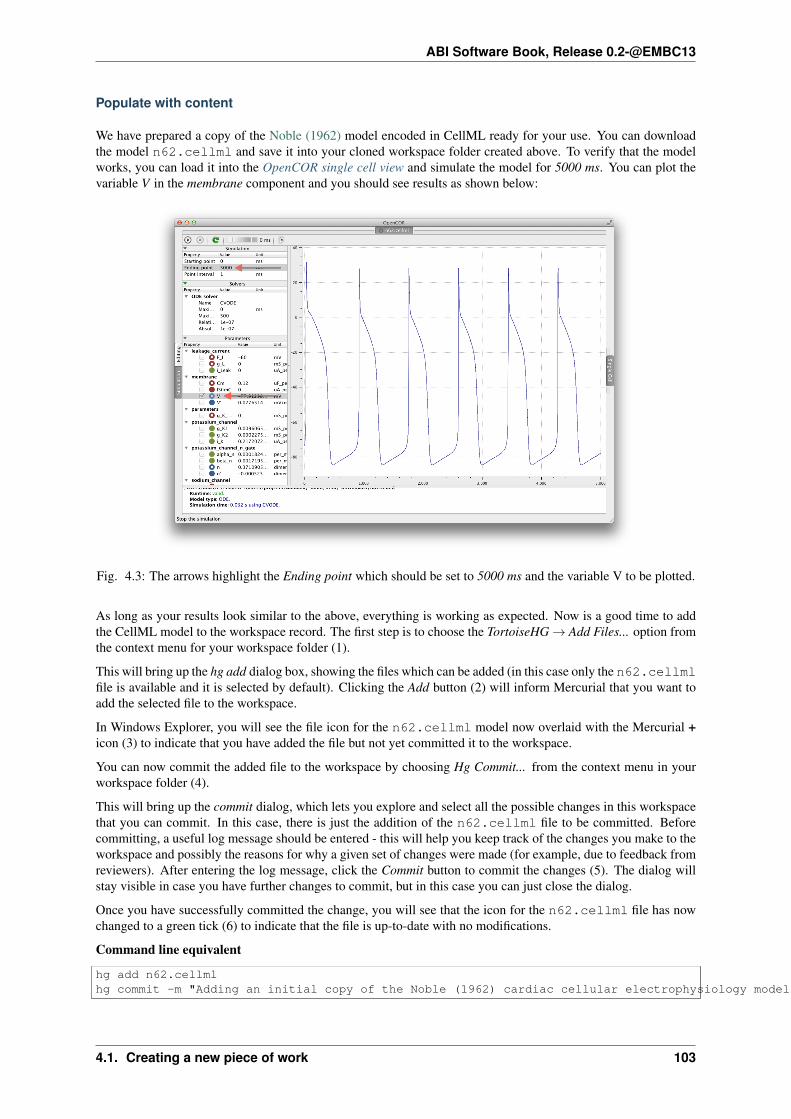
ABI Software Book, Release 0.2-@EMBC13
Populate with content
We have prepared a copy of the Noble (1962) model encoded in CellML ready for your use. You can downloadthe model n62.cellml and save it into your cloned workspace folder created above. To verify that the modelworks, you can load it into the OpenCOR single cell view and simulate the model for 5000 ms. You can plot thevariable V in the membrane component and you should see results as shown below:
Fig. 4.3: The arrows highlight the Ending point which should be set to 5000 ms and the variable V to be plotted.
As long as your results look similar to the above, everything is working as expected. Now is a good time to addthe CellML model to the workspace record. The first step is to choose the TortoiseHG → Add Files... option fromthe context menu for your workspace folder (1).
This will bring up the hg add dialog box, showing the files which can be added (in this case only the n62.cellmlfile is available and it is selected by default). Clicking the Add button (2) will inform Mercurial that you want toadd the selected file to the workspace.
In Windows Explorer, you will see the file icon for the n62.cellml model now overlaid with the Mercurial +icon (3) to indicate that you have added the file but not yet committed it to the workspace.
You can now commit the added file to the workspace by choosing Hg Commit... from the context menu in yourworkspace folder (4).
This will bring up the commit dialog, which lets you explore and select all the possible changes in this workspacethat you can commit. In this case, there is just the addition of the n62.cellml file to be committed. Beforecommitting, a useful log message should be entered - this will help you keep track of the changes you make to theworkspace and possibly the reasons for why a given set of changes were made (for example, due to feedback fromreviewers). After entering the log message, click the Commit button to commit the changes (5). The dialog willstay visible in case you have further changes to commit, but in this case you can just close the dialog.
Once you have successfully committed the change, you will see that the icon for the n62.cellml file has nowchanged to a green tick (6) to indicate that the file is up-to-date with no modifications.
Command line equivalent
hg add n62.cellmlhg commit -m "Adding an initial copy of the Noble (1962) cardiac cellular electrophysiology model to the workspace."
4.1. Creating a new piece of work 103

ABI Software Book, Release 0.2-@EMBC13
104 Chapter 4. Developing the Virtual Physiological Human

ABI Software Book, Release 0.2-@EMBC13
4.1. Creating a new piece of work 105

ABI Software Book, Release 0.2-@EMBC13
While we have the model open in OpenCOR, we should have a go at annotating some of the variables in themodel. Full instructions for this can be found in the OpenCOR CellML annotation view. First, we will follow theexample given in those instructions for annotating the sodium_channel component.
The first step is to switch to the Editing mode (1) and select the sodium_channel component for annotation(2). We will be using the bio:isVersionOf as the qualifier for this annotation (3) and searching for termsrelated to sodium (4).
We can then add desireable terms from the search results by choosing the + button beside the term to add to theannotations for the sodium_channel component (5).
Have a play annotating other variables and components in the model. When done annotating, make sure to savethe model (File → Save). With the CellML model updated, now is a good time to commit the changes to the
106 Chapter 4. Developing the Virtual Physiological Human

ABI Software Book, Release 0.2-@EMBC13
workspace.
As above, choose Hg Commit... from the context menu in your workspace folder to bring up the Mercurial commitdialog. This time you will see that there is one file modified that can be committed, n62.cellml (1). As wementioned previously, it is important to enter a good log message to keep a record of the changes you make (2),and the changes made to the currently selected file are shown to help remind you as to your changes (3). In thiscase, OpenCOR has made many changes to the whitespace in the file, as well as adding the RDF annotations atthe bottom of the file.
Command line equivalent
hg diffhg commit -m "Using OpenCOR to add some annotations to my copy of the Noble 1962 model."
Push back to the repository
Having added content and performed some modifications, it is time to push the changes back to the model repos-itory, achieved in TortoiseHG with the synchronization action. First, select TortoiseHG → Synchronize from thecontext menu for your workspace folder.
This will bring up the TortoiseHG Sync dialog. In this dialog, you will see that by default you will be synchronizingwith the workspace on the teaching repository from which you originally created this clone. This is usually whatyou want to do, but it is possible to synchronize with other Mercurial repositories. In this case, we want to push thechanges we have made to the model repository, so choose the corresponding action from the toolbar (highlightedbelow).
Once you choose the push action, you will be asked to confirm that you want to push to your remote repositoryand then asked for your username and password (these are the credentials you created when registering for anaccount in the model repository). You will then see a listing of the transaction as your changes are pushed to therepository and a message stating the push has completed.
Command line equivalent
hg push
If you now return to browsing your workspace in your web browser, and refresh the page, you will see that yourworkspace now has some content - n62.cellml - and if you view the workspace history you will see the logmessages that you entered when committing your changes above.
4.1. Creating a new piece of work 107
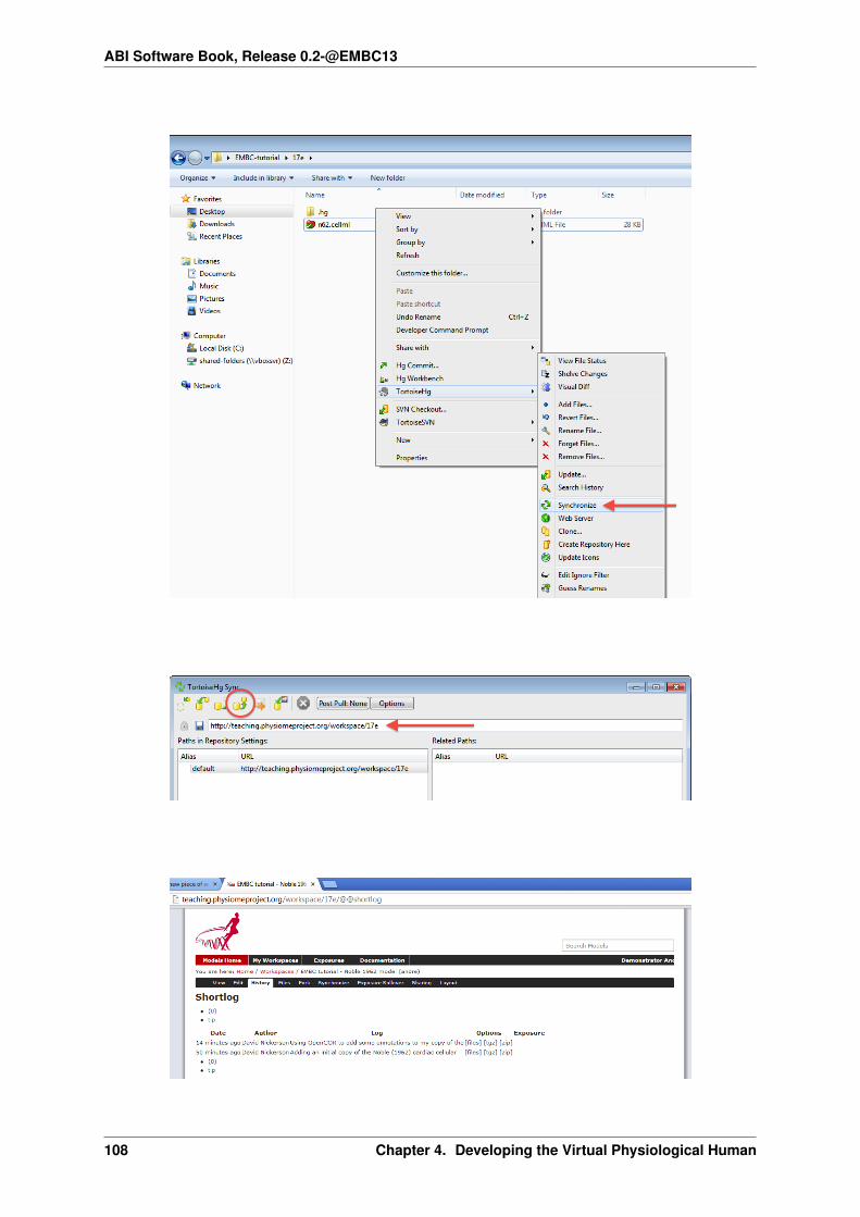
ABI Software Book, Release 0.2-@EMBC13
108 Chapter 4. Developing the Virtual Physiological Human

ABI Software Book, Release 0.2-@EMBC13
Now might be a good time to think about sharing your workspace with your neighbors. You might also want tohave a look at creating an exposure for your workspace. To learn how to create exposures, please refer to CreatingCellML exposures.
4.1.3 A new image segmentation study
In this part of the tutorial, we use the MAP client software to create a new workflow which will take a set ofimages, from the model repository, and apply an automated image segmentation algorithm to them which willproduce a data point cloud.
Before beginning this tutorial, you need to have the MAP client installed on your machine. Please follow the MAPInstallation and Setup Guide.
The remainder of this tutorial can be found in the MAP documentation, MAP Tutorial - Create Workflow.
4.1.4 Best practice tips
TodoComplete this section
Creating a new piece of work from scratch -> encouraging best practices!
• create workspace, commit often, useful log messages
• provenance data (making sure user name/ID is set correctly)
• share directly with collaborators
• annotation?
• creating exposures? link through to PMR documentation...?
4.2 Reproducing published data
In the Physiome Model Repository (PMR), a complete piece of work is stored in a workspace. Each workspaceis a Mercurial repository, which allows PMR to maintain a complete history of all changes made to every file itcontains. In this tutorial, we take you through the process of reproducing an existing piece of “published” work -commonly, the first stage in establishing a new project which builds on previous discoveries.
4.2.1 Reproducing model behavior in OpenCOR
In this tutorial, we will be demonstrating how to reproduce the results from a CellML model as they were originallypublished. Because the Physiome Model Repository makes use of Mercurial, even if a workspace has continuedbeing developed after a particular revision is published, we are able to step back through the workspace history toreproduce those original published results.
Following on from the previous tutorial, we make use of the Noble (1962) cardiac cellular electrophysiologymodel. In this tutorial, we will use the version of this model published in the CellML model repository andavailable here: http://models.cellml.org/e/174. If you navigate from that exposure to the workspace you can checkthe history as shown below.
As you can see highlighted in the Exposure column of the history above, there are two exposures for thisworkspace. For the purposes of this tutorial, we will assume that the earlier exposure corresponds to a studythat has been published in a scientific journal. The later exposure is the result of further work on this modelfollowing the publication of the journal article. The later exposure illustrates the difference between these twoversions of the model. In this tutorial, we aim to reproduce the results as shown in the published journal article -corresponding to the earlier exposure.
4.2. Reproducing published data 109
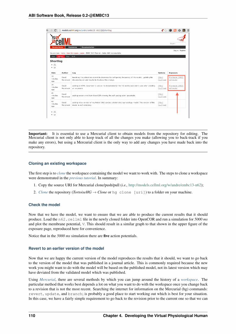
ABI Software Book, Release 0.2-@EMBC13
Important: It is essential to use a Mercurial client to obtain models from the repository for editing. TheMercurial client is not only able to keep track of all the changes you make (allowing you to back-track if youmake any errors), but using a Mercurial client is the only way to add any changes you have made back into therepository.
Cloning an existing workspace
The first step is to clone the workspace containing the model we want to work with. The steps to clone a workspacewere demonstrated in the previous tutorial. In summary:
1. Copy the source URI for Mercurial clone/push/pull (i.e., http://models.cellml.org/w/andre/embc13-n62);
2. Clone the repository (TortoiseHG → Clone or hg clone [uri]) to a folder on your machine.
Check the model
Now that we have the model, we want to ensure that we are able to produce the current results that it shouldproduce. Load the n62.cellml file in the newly cloned folder into OpenCOR and run a simulation for 5000 msand plot the membrane potential, V. This should result in a similar graph to that shown in the upper figure of theexposure page, reproduced here for convenience.
Notice that in the 5000 ms simulation there are five action potentials.
Revert to an earlier version of the model
Now that we are happy the current version of the model reproduces the results that it should, we want to go backto the version of the model that was published in a journal article. This is commonly required because the newwork you might want to do with the model will be based on the published model, not its latest version which mayhave deviated from the validated model which was published.
Using Mercurial, there are several methods by which you can jump around the history of a workspace. Theparticular method that works best depends a lot on what you want to do with the workspace once you change backto a revision that is not the most recent. Searching the internet for information on the Mercurial (hg) commands:revert, update, and branch; is probably a good place to start working out which is best for your situation.In this case, we have a fairly simple requirement to go back to the revision prior to the current one so that we can
110 Chapter 4. Developing the Virtual Physiological Human
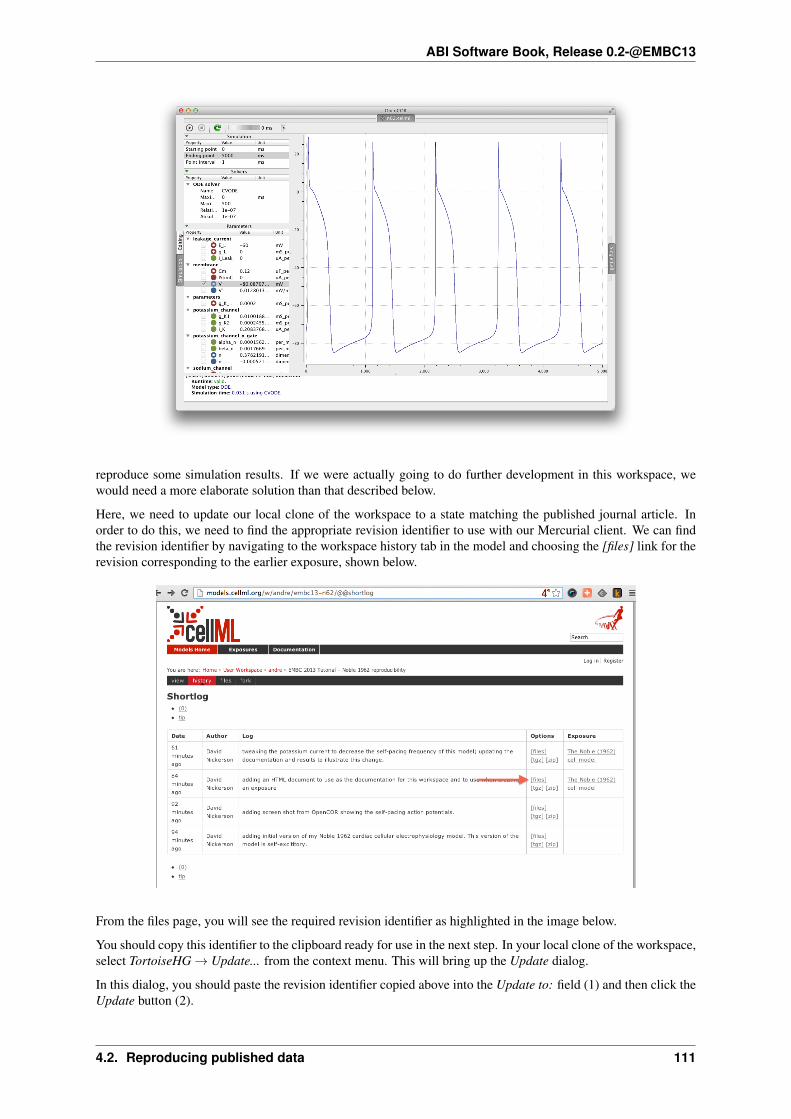
ABI Software Book, Release 0.2-@EMBC13
reproduce some simulation results. If we were actually going to do further development in this workspace, wewould need a more elaborate solution than that described below.
Here, we need to update our local clone of the workspace to a state matching the published journal article. Inorder to do this, we need to find the appropriate revision identifier to use with our Mercurial client. We can findthe revision identifier by navigating to the workspace history tab in the model and choosing the [files] link for therevision corresponding to the earlier exposure, shown below.
From the files page, you will see the required revision identifier as highlighted in the image below.
You should copy this identifier to the clipboard ready for use in the next step. In your local clone of the workspace,select TortoiseHG → Update... from the context menu. This will bring up the Update dialog.
In this dialog, you should paste the revision identifier copied above into the Update to: field (1) and then click theUpdate button (2).
4.2. Reproducing published data 111
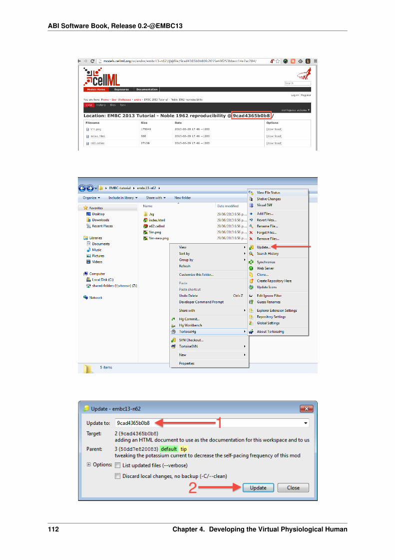
ABI Software Book, Release 0.2-@EMBC13
112 Chapter 4. Developing the Virtual Physiological Human

ABI Software Book, Release 0.2-@EMBC13
Command line equivalent
hg update -r 9cad4365b0b8
You will now see in your local clone that the files have reverted back to that previous version. Loading this versionof n62.cellml into OpenCOR and simulating for 5000 ms should result in the figure matching that presentedin the earlier exposure page and reproduced here for convenience.
Note in particular that there should now be the same six action potentials that were present in the published versionof the model.
4.2.2 Recreating a published image segmentation study
In the previous MAP tutorial you created a new workflow for segmenting a set of images. In this scenario, weimagine that someone has previously published a similar study also using the MAP client and PMR. You cansee an exposure for such an example here: http://teaching.physiomeproject.org/e/190/. In this tutorial, we use theMAP client to reproduce this study.
Import workflow
To recreate this published workflow, we need to import it into the MAP client. To do this, in the MAP client selectFile → Import. This first step is to provide a folder in which to store the workflow on your local machine. Youshould create a new folder for this workflow. You will then be presented with the MAP PMR tool, you will need tomake sure you have registered the MAP client with PMR. In the PMR tool you are able to search for the worklowyou would like to import from the repository. In this case, search for the term autosegmenter (1). You willsee there is only one result (2) which you should select and the click the OK button.
This will import the workflow from the repository to your local folder and you should then see the workflow asshown in the exposure page referenced above. If you have the MAP client and plugins all working correctly,clicking Execute should result in an interactive view of the segmented data, as also shown on the exposure pagereferenced above.
Note: When saving changes in the MAP client currently, they are automatically saved to the workspace andpushed to the repository. In this example you will not have permission to push into the repository. This is a knownlimitation in the MAP client at present.
4.2. Reproducing published data 113

ABI Software Book, Release 0.2-@EMBC13
4.2.3 Best practice tips
TodoThis section.
Some tips for best practice:
• It is essential to use a Mercurial client to obtain models from the repository for editing. The Mercurialclient is not only able to keep track of all the changes you make (allowing you to back-track if youmake any errors), but using a Mercurial client is the only way to add any changes you have made backinto the repository. Some tools, like MAP, will hide the Mercurial details from the user.
• By making your work publicly available in standard formats you significantly enhance the ability ofother scientists to make use of your work. Similarly, when embarking on a new study it is worthchecking the various repositories for existing work that you might be able to build on - such workshould normally be discovered during a literature search.
4.3 Find an existing piece of work and extend it
In the preceeding tutorials, you have learnt how to create a new piece of work from scratch using the PhysiomeModel Respository and how to reproduce a “published” result. In this tutorial, we will demonstrate how to takean exisiting piece of work, stored in a public workspace, and develop it further to address a new goal.
4.3.1 Extending an existing CellML model
In this part of the tutorial, we will once again be making use of the Noble (1962) cardiac cellular electrophysiologymodel. We will be taking the model and making changes to alter its behaviour. For this, we will be using the ver-sion of the model published in the teaching instance of the repository: http://teaching.physiomeproject.org/e/183,but the process described below will also work in the main repository site.
Forking an existing workspace
Important: It is essential to use a Mercurial client to obtain models from the repository for editing. The
114 Chapter 4. Developing the Virtual Physiological Human

ABI Software Book, Release 0.2-@EMBC13
Mercurial client is not only able to keep track of all the changes you make (allowing you to back-track if youmake any errors), but using a Mercurial client is the only way to add any changes you have made back into therepository.
For this tutorial, we will fork an existing workspace. This creates a new workspace owned by you, containing acopy of all the files in the workspace you forked including their complete history. This is equivalent to cloningthe workspace, creating a new workspace for yourself, and then pushing the contents of the cloned workspace intoyour new workspace.
Forking a workspace can be done using the Physiome Model Repository web interface. The first step is to findthe workspace you wish to fork. We will use the EMBC 2013 Tutorial - Noble 1962 workspace from the exposurereferenced above, which can be found at: http://teaching.physiomeproject.org/workspace/182.
Now click on the fork option in the toolbar, as shown below (1).
You will be asked to confirm the fork action by clicking the Fork button (2). You will then be shown the page foryour forked workspace.
Cloning your forked workspace
In order to make changes to your workspace, you have to clone it to your own computer. To do this, follow theprocedure as described in the earlier tutorial.
Quietening the self excitation
The version of the Noble 1962 model you have just forked and cloned is a model of a Purkinje fibre cell. Thesecells are capable of acting as pacemaker cells, although usually entrained by the sinoatrial node of the heart. TheNoble model reproduces this behavior but is also able to simulate a non-pacing version of the cell model. This isaccomplished by decreasing the potassium current which gives rise to the gradual depolarization of the memberpotential seen the figures from OpenCOR for the model in the previous tutorials. Once the cell is in a quiesentstate, we are able to then apply an electrical stimulus to impose our own pacing regime.
If you load the n62.cellml file from the workspace you have just cloned into OpenCOR, set the duration of thesimulation to 5000 ms, and plot the membrane potential V, you will be able to see the effect of altering the valueof the variable g_K_add in the parameters component. As you increase this value you should see the restingpotential decrease and the abolution of the self-exciting mechanism. A value of 0.001 mS_per_mmsq keeps theresting potential in the physiological range and makes the cell quiesent.
The version of OpenCOR we are using in this tutorial will not save the modified parameter value, so you will needto open the n62.cellml file in a text editor and make the change manually. In your text editor search for theg_K_add variable in the parameters component, as shown below.
Set the initial_value attribute to the value you determined most suitable in OpenCOR. Reload the modelinto OpenCOR to confirm that the results are as expected, hopefully something similar to those shown below.
Now would be a good time to commit your changes to your clone of the workspace
4.3. Find an existing piece of work and extend it 115
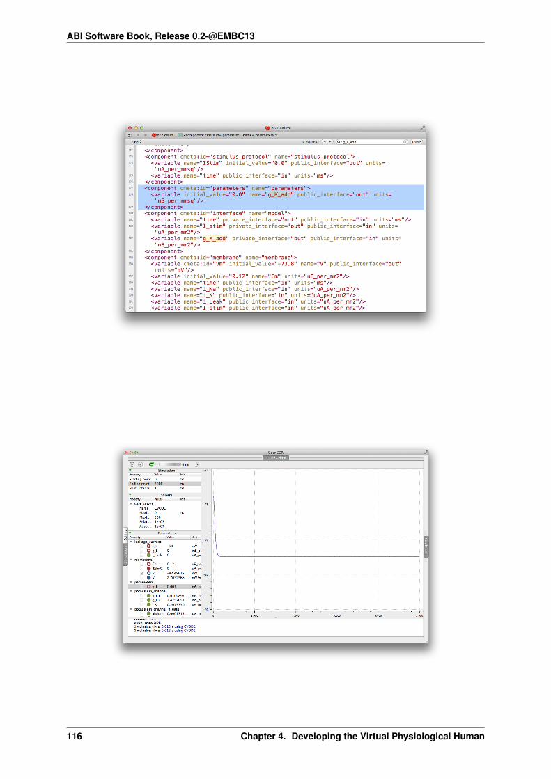
ABI Software Book, Release 0.2-@EMBC13
116 Chapter 4. Developing the Virtual Physiological Human
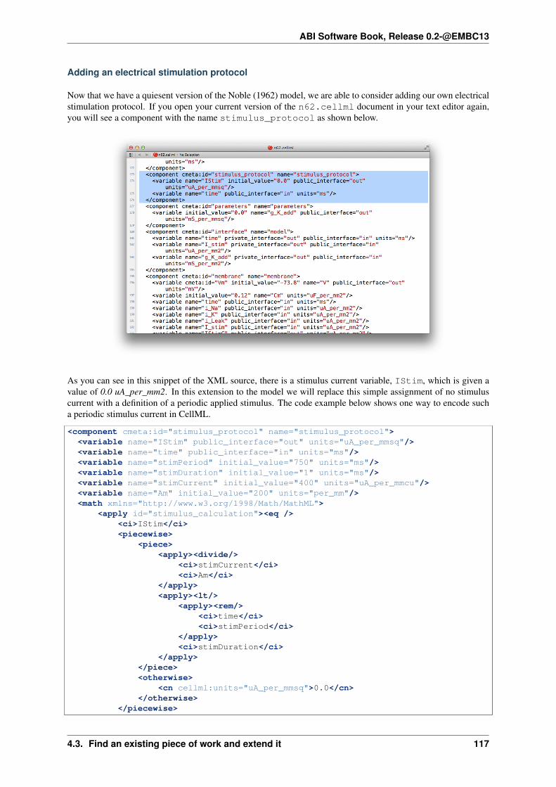
ABI Software Book, Release 0.2-@EMBC13
Adding an electrical stimulation protocol
Now that we have a quiesent version of the Noble (1962) model, we are able to consider adding our own electricalstimulation protocol. If you open your current version of the n62.cellml document in your text editor again,you will see a component with the name stimulus_protocol as shown below.
As you can see in this snippet of the XML source, there is a stimulus current variable, IStim, which is given avalue of 0.0 uA_per_mm2. In this extension to the model we will replace this simple assignment of no stimuluscurrent with a definition of a periodic applied stimulus. The code example below shows one way to encode sucha periodic stimulus current in CellML.
<component cmeta:id="stimulus_protocol" name="stimulus_protocol"><variable name="IStim" public_interface="out" units="uA_per_mmsq"/><variable name="time" public_interface="in" units="ms"/><variable name="stimPeriod" initial_value="750" units="ms"/><variable name="stimDuration" initial_value="1" units="ms"/><variable name="stimCurrent" initial_value="400" units="uA_per_mmcu"/><variable name="Am" initial_value="200" units="per_mm"/><math xmlns="http://www.w3.org/1998/Math/MathML">
<apply id="stimulus_calculation"><eq /><ci>IStim</ci><piecewise>
<piece><apply><divide/>
<ci>stimCurrent</ci><ci>Am</ci>
</apply><apply><lt/>
<apply><rem/><ci>time</ci><ci>stimPeriod</ci>
</apply><ci>stimDuration</ci>
</apply></piece><otherwise>
<cn cellml:units="uA_per_mmsq">0.0</cn></otherwise>
</piecewise>
4.3. Find an existing piece of work and extend it 117

ABI Software Book, Release 0.2-@EMBC13
</apply></math>
</component>
In the above example, we have introduced some new variable to control the frequency, duration, and magnitudeof the applied stimulus current. If you replace the stimululs_protocol component in the n62.cellmlmodel with the one above, you are able to load the new version of the model into OpenCOR and have a play withthose variables to ensure they are behaving as expected. Note: you may need to set the Maximum step for CVODEto 0.1 or change to the Forward Euler integrator in OpenCOR to ensure that your specified stimulus in correctlydetected by the numerical integration scheme.
Now would be a good time to commit your changes to your clone of the workspace and push them back to themodel repository. You might also want to think about sharing your workspace with your neighbors or to havea look at creating an exposure for your workspace. To learn how to create exposures, please refer to CreatingCellML exposures.
4.3.2 Wrapping your favorite tool as a MAP client plugin
The MAP framework is a very general purpose workflow-based tool. By taking advantage of the collaborativedevelopment and sharing features of the Physiome Model Repository, you have seen in the previous MAP tutorialhow it is possible to share your work in a manner that makes it easy for other scientists to utilise and extend.
With the plugin approach used by the MAP client software, it is possible to wrap you favorite software tools tomake them available as steps in a MAP workflow. For example, the previous tutorials have made use of the Zincvisualisation and field manipulation library.
The process of developing a MAP plugin is beyond the scope of this tutorial. If you are interested, there is thebeginnings of some documentation for this process which will be developing in the near future. There is also askeleton plugin that comes the MAP client software (in the plugins folder) which serves as the starting pointfor developing any new plugin and the github project which will contain a collection of MAP plugins. If you areinterested in developing a plugin or would like help wrapping your favorite tool as a workflow step, please don’thesitate to contact the MAP team (or talk to Hugh today!).
4.3.3 Best practice tips
TodoComplete this section
Creating a new piece of work from scratch -> encouraging best practices!
• create workspace, commit often, useful log messages
• provenance data (making sure user name/ID is set correctly)
• share directly with collaborators
• annotation?
• creating exposures? link through to PMR documentation...?
118 Chapter 4. Developing the Virtual Physiological Human
CHAPTER 5
Related Software Project at the Auckland Bioengineering Institute
Contents:
5.1 Cmgui user documentation
This documentation provides an overview of the functionality of the cmgui application, as well as some informa-tion about the architecture of the software, and some of the concepts behind the visualizations.
This documentation is current for cmgui version 2.9.0.
5.1.1 Migration documentation for users of previous versions
Some of the changes in recent versions of cmgui will cause some old commands to break - changes may need tobe made to some old command files. Below are links to documents detailing these changes.
Changes in recent versions
Migrating to Cmgui 2.8
Scenes and graphics filters The biggest change in cmgui 2.8 is that graphics are now associated with regionsand not stored in a separate ‘scene graph’. The Scene Editor displays the region tree, and each region has agraphical ‘rendition’ consisting of a list of graphics (lines, surfaces, node_points etc.) which visualize the fields ofthat region. This change should not affect most users, because previous versions of cmgui made the scene graphmirror the flat list of regions and groups used in most models and the commands to set up these graphics shouldwork as before.
However, if your command file created new scenes (or modified certain attributes of scene ‘default’), or yourmodel consisted of more than just a simple list of regions and groups (i.e. regions within regions within the rootregion) you will need to make some changes.
Rendition or ‘graphical element’ Since graphics now belong to a region, the commands to create them nowtake the region path instead of the name of the ‘graphical element’ (now termed ‘rendition’) on a particular scene:
gfx modify g_element REGION_PATH ...
Argument scene NAME is now redundant and ignored. Since the automatic name for the ‘g_element’ was theregion or group name, most previous commands work as before.
119

ABI Software Book, Release 0.2-@EMBC13
Scenes Scenes remain as the objects determining which graphics are displayed in a window or exported byvarious commands. However they are considerably simplified in that their main attributes are (1) the top regionthey show graphics for and (2) A graphics ‘filter’ object which controls which graphics from the region tree arevisible (see later).
The command for creating or modifying a scene is as follows:
Usage : gfx define scene ??SCENE_NAME
<add_light LIGHT_NAME|none[none]><region PATH_TO_REGION[/]><remove_light LIGHT_NAME|none[none]><filter GRAPHICS_FILTER_NAME|none[none]>
(gfx modify scene is the same as gfx define scene. Note future plans are to remove lights fromscenes and list them as special graphics as part of a rendition.)
The gfx create scene command has been removed because invariably the command file must be manuallyupdated to replace it, and it is now no longer necessary to create ‘child’ scenes to make hierarchical graphics.Cmgui developers are happy to help with migration.
Graphics filters Graphics filters are new objects which control which graphics are shown in a scene. Each filterhas a criterion for matching attributes of a graphic or region/rendition, and if the result is true the graphic is shown.The initial graphics types include:
• matching visibility flags
• matching graphic name
• matching (within) region path
• logical operator OR
• logical operator AND
Furthermore, all criteria can be inverted to create logical not:
Usage : gfx define graphics_filter ??GRAPHICS_FILTER_NAME
* Filter to set up what will be and what will not be
* included in a scene. The optional inverse_match flag
* will invert the filter's match criterion. The behaviour
* is to show matching graphic with the matching criteria.
* <match_graphic_name> filters graphic with the matching
* name. <match_visibility_flags> filters graphic with
* the setting on the visibility flag. <match_region_path>
* filters graphic in the specified region or its subregion.
* <operator_or> filters the scene using the logical operation
* 'or' on a collective of filters. <operator_and> filters
* the scene using the logical operation 'and' on a collective
* of filters. Filters created earlier can be added or
* removed from the <operator_or> and <operator_and> filter.<operator_or
<add_filters[add_filters]|remove_filters>FILTER_NAMES >
<operator_and<add_filters[add_filters]|remove_filters>
FILTER_NAMES ><match_graphic_name MATCH_NAME><match_visibility_flags><match_region_path REGION_PATH><inverse_match|normal_match[normal_match]>
The default filter matches the familiar visibility flags of the region/rendition and each graphic:
120 Chapter 5. Related Software Project at the Auckland Bioengineering Institute

ABI Software Book, Release 0.2-@EMBC13
gfx define graphics_filter default normal_match match_visibility_flags;
The following makes a filter that shows all graphics satisfying the above default OR if graphics is named “bob”:
gfx define graphics_filter bob normal_match match_graphic_name "bob";gfx define graphics_filter default_or_bob normal_match operator_or add_filters default bob;gfx define scene default filter default_or_bob;
Note it is easy for us to add new filter types as needed by users.
Drawing static graphics Cmgui now associates all graphics with a region rather than a separate ‘scene graph’,so all previous commands to create and draw ‘static’ graphics on a scene are removed or changed. The equivalentfunctionality is achieved by adding a ‘point’ graphic to a region rendition in the scene editor, which can show anyglyph with controllable scale, offset, material and optional label. The commands for reproducing the graphics canbe obtained using gfx list g_element REGION_PATH commands.
• gfx create axes now just writes a migration note as it is redundant. Several axes objects are prede-fined in the glyph list to be used with point graphics. See comment on gfx draw below.
• gfx create annotation has been removed. You must now define a string field in the respective re-gion with the required text (gfx define field ![REGION_PATH/]NAME string constant"Your text here") and use it as a label, probably with glyph none, on a point graphic.
• gfx create colour_bar works as before but the colour bar is now put in the list of glyphs able to beshown with any point graphic.
• gfx create lines/surfaces/node_points ... have been removed altogether. You must nowuse gfx modify g_element REGION_PATH lines/surfaces/node_points ....
• ‘gfx draw’ now creates a point graphic in the root region rendition with the glyph matching the graphicsname specified. If you had previously created axes with the default name “axes” it finds the glyph howeverthe scaling, offset and material are lost: edit these in the scene editor. The scene is ignored by this commandso you will need to make changes if you were drawing to multiple scenes, particularly an overlay scene (seemigration notes for overlay graphics below).
• ‘gfx erase’ has been removed.
Overlay graphics and coordinate systems Previous versions of cmgui required an ‘overlay scene’ attribute tobe set for each graphics window. Any graphics drawn in the selected overlay scene were drawn in a window-relative coordinate system on that window.
This has been replaced by a far simpler and more powerful mechanism. Each graphic in the scene editor has a‘graphics coordinate system’ which can be:
• LOCAL = subject to the graphical transformations of the renditions in the region tree relative to world (thedefault).
• WORLD = in the world coordinate system of the top region of the scene
• NORMALISED_WINDOW_FILL = ranges from ![-1,+1] across all dimension of window so distorting ifwindow is non-square. This was the mode used by the overlay scene.
• NORMALISED_WINDOW_FIT_LEFT/RIGHT/BOTTOM/TOP = ranges from ![-1,+1] in the largestsquare fitting in the window, aligned to the specified side. Non-distorting so perferable to NOR-MALISED_WINDOW_FILL.
• WINDOW_PIXEL_BOTTOM_LEFT/TOP_LEFT = In screen pixels from (0,0) at the specified origin ofthe window, with +x to the right, +y up. TOP_LEFT has negative y coordinates on screen.
Choosing any window-relative coordinate system causes the graphic to be drawn as an overlay, i.e. on top of allnon-overlay graphics, on rendering windows. Window-relative graphics cannot be exported to VRML and otherformats without a viewport.
5.1. Cmgui user documentation 121

ABI Software Book, Release 0.2-@EMBC13
Future plans are to allow layers to be specified independently from the graphics coordinate system, with layers‘background’, ‘default’ and ‘overlay’ predefined and the ability to add more layers and control whether the depthbuffer is cleared between layers.
Removal of ‘general settings’ for graphics In previous versions of cmgui, the graphical rendition of a region(g_element commands) had a set of ‘general settings’ controlling the ‘discretisation’ (number of line segmentsused to approximate curved element boundaries), and also a default coordinate field to apply to graphics which donot have the coordinate field specified.
For cmgui 2.8 all these general settings have been removed and must be specified for each graphic in the ren-dition. This has the benefit of allowing different graphics to use different discretisations, which are now set via‘tessellation’ objects (see later).
To minimize migration issues, all previous gfx modify g_element REGION_PATH general ... op-tions are read and become defaults for subsequent g_element commands to add graphics. If the general ‘ele-ment_discretization’ attribute is set then on creating new graphics requiring a tessellation it finds or creates onegiving the same effect as the discretization; it will have an automatically generated name such as ‘temp2’. Chang-ing these general options now has no effect on graphics that have already been created. The only non-deprecatedg_element general command option is to clear all graphics from the rendition.
Note that region renditions still have transformation attributes which give the 4x4 transformation from local toparent coordinate systems.
Tessellation Tessellation objects have been introduced to replace the general ‘element_discretization’ attributeand solve several problems:
• they allow any number of graphics – and not just from the same region – to share tessellation settings,allowing graphics quality across complicated model visualisations to be changed from a few controls.
• they allow tessellation quality to automatically switch from minimum for linear basis functions to fine fornon-linear bases and coordinate systems. (Note: bilinear and trilinear Lagrange are considered linear eventhough they have a few quadratic or cubic product terms.)
• we anticipate adding more options in future e.g. adaptive curvature-dependent triangulation, but graphicswill still only require one object to be chosen.
However, tessellation objects do not solve one problem, that choosing a very large number causes Cmgui to lockup while all affected graphics are regenerated: take care when setting large values!
Note that elements_points and streamlines do not have a tessellation object set by default. Instead they have aseparate fixed ‘discretization’ setting which defaults to “1*1*1” (i.e. 1 point or streamline per element), but youmay add a tessellation which then acts as a multiplier on the discretization. The optional native_discretizationfield also acts as a multiplier.
Commands for defining tessellations are:
Usage : gfx define tessellation ??TESSELLATION_NAME
* Defines tessellation objects which control how finite
* elements are subdivided into graphics. The minimum_divisions
* option gives the minimum number of linear segments
* approximating geometry in each xi dimension of the
* element. If the coordinate field of a graphic uses
* non-linear basis functions the minimum_divisions is
* multiplied by the refinement_factors to give the refined
* number of segments. Both minimum_divisions and refinement_factors
* use the last supplied number for all higher dimensions,
* so "4" = "4*4" and so on.<minimum_divisions "#*#*..."["1"]{>=0}><refinement_factors "#*#*..."["1"]{>=0}>
You can also list all available tessellations with:
122 Chapter 5. Related Software Project at the Auckland Bioengineering Institute

ABI Software Book, Release 0.2-@EMBC13
gfx list tessellation
The default tessellation exists from start-up, but can be edited:
gfx define tessellation default minimum_divisions "1" refinement_factors "4";
A tessellation editor dialog can be opened by clicking on the “Edit...” button beside the tessellation chooser in thescene editor.
Migrating to Cmgui 2.9
In the 2.9.0 release, significant changes have been made to the way ‘groups’ are handled. We have also removedthe automatic creation of default lines on reading a model.
While we’ve taken every effort to minimise the impact of the changes, usually by making commands do the nearestequivalent behaviour, some breaks are unavoidable. So if your command files are not working as before, pleasetry to see why in the following explanation, but if that doesn’t help, see the Cmgui development team. As always,if you find what looks like a bug in the software, please report it on our tracker.
Removal of ‘group regions’
Background A Cmgui model is made up of a tree of objects called regions, each of which owns a set of nodes,elements, data points (an extra set of nodes) and fields defined on them, plus 0 or more child regions. Regions arelike the folders in a file system; fields (and other ‘intra region’ objects such as sets of nodes and meshes) are likefiles in the folder. The root region is denoted by “/”, and region names in a path are separated by “/”.
A ‘group’ is a subset of the nodes, elements and data points owned by a region. Prior to this release, each groupwas created as a pseudo region, what we called a ‘group region’. This meant they looked like a region exceptthey contained a subset of the objects of the parent/master region, and listed all fields of the master region (butcould only address those defined over its subset). This also meant every group could individually have graphicsassociated with it. For users, the downsides of group regions were that they hid away the definitions of theirsubgroups so it was not possible to intersect or union them in field expressions, it was not possible to makeinvisible subgroups (they all had a graphical rendition), and it was impossible to make hierarchical groups andgroups containing whole regions. For developers they have been a maintenance hazard and a feature we did notwish to expose to our API.
The Change From Cmgui 2.9, groups are implemented as fields. A group field returns 1 at any location in thedomain (at nodes, in elements etc.) which is in the group, 0 elsewhere. From the API you can add the wholeregion to a group, but this is not available through gfx commands. Group fields can have subregion groups in childregions, so a group tree can contain an arbitrary subset of a region tree. The group field can have zero or more‘subobject group fields’ representing subsets of specific object types that are present in the group, each of whichgive the value 1 on the respective object type in the group, 0 otherwise. For example, if you read cube example a2and write “gfx list fields” you will now see 5 new fields:
cube : group = generic group objectcube.cmiss_mesh_1d : sub_group_object = subset of "cmiss_mesh_1d" in group cubecube.cmiss_mesh_2d : sub_group_object = subset of "cmiss_mesh_2d" in group cubecube.cmiss_mesh_3d : sub_group_object = subset of "cmiss_mesh_3d" in group cubecube.cmiss_nodes : sub_group_object = subset of "cmiss_nodes" in group cube
Note: In several new commands, “cmiss_nodes” is the name you use to reference the set of nodes in the region,“cmiss_data” references the set of data points, and “cmiss_mesh_Nd” references the 1, 2 and 3-D meshes ownedby that region. In future we anticipate allowing any number of meshes to be created with their own names.
Since Cmgui 2.8, when you select objects in the graphics window, you are making a group which is automaticallygiven the name “cmiss_selection”, and any selected objects are added to subobject groups coordinated under it.For example, selecting a face element of the cube creates:
5.1. Cmgui user documentation 123

ABI Software Book, Release 0.2-@EMBC13
cmiss_selection : groupcmiss_selection.cmiss_mesh_2d : sub_group_object
There is now only one type of group; the previous group regions and the selection have been merged into the sameclass.
Prefer Regions to Groups Shortly we will explain several of the workarounds that make most existing com-mand files work as before, most of the time. But first we wish to recommend using regions instead of groupswhenever possible, and if you can do this your command files will likely work just as before. Needlessly using agroup means all your objects are listed twice, once for the region and once for the group, which consumes morememory. To migrate to regions, just change lines in EX files from:
Group name: NAME
to (and the leading "/" is required):
Region: /NAME
(The Region can have a full path e.g. /bob/fred; the group is just a name which is within the namespace of thesurrounding region. At the start of parsing EX files, the file’s root region “/” is active.)
Another approach is to specify the region on the read command “gfx read node/element/data region PATH”, butbear in mind this will continue to create groups at the named path. This effectively maps the file’s root region tothe named region.
Warning: Be aware that there are still cases where you can’t use regions, so continued use of groups will benecessary:
1. Whenever several element groups share common nodes. Elements can only reference nodes from thesame region.
2. Certain features such as the compose/find_mesh_location fields that do not work inter-region.We certainly wish to remedy these in time. We need to hear user input about what functionality they need towork between regions.
Possible breaks with the removal of group regions 1. Groups no longer have a rendition
Each region has a ‘rendition’ which is the set of graphics for visualising its fields. When groups were presentedas regions, they too had their own rendition. We now interpret existing commands in the form:
gfx modify g_element [REGION_PATH]/GROUP_NAME ...
as:
gfx modify g_element [REGION_PATH]/ ... subgroup GROUP_NAME
Hence the graphics now belong to the parent region. All graphics now have an optional subgroup field and whensupplied only shows primitives for which the field is non-zero. Hence the new group fields are all usable, but so isany other scalar field expressions (e.g. less_than(mag(coordinates), 100.0). When you re-list graphics with “gfxlist g_element” you will see the new form. Note: this also replaces the “visibility_field” option on node_pointsand data_points so you will need to rename this.
The “gfx modify g_element [REGION_PATH]/GROUP_NAME” command clears only graphics using the groupof the GROUP_NAME as the subgroup field. Beware that clearing the graphics of the parent region will also clearthose referencing any subgroup.
2. Groups no longer have a rendition, hence have no individual ‘default’ arguments
Cmgui 2.8 (the last public release) deprecated all arguments to the “general” command for modifying graphicsexcept for the clear command.
gfx modify g_element PATH general clear default_coordinate NAME element_discretization “#*#*...” ...
124 Chapter 5. Related Software Project at the Auckland Bioengineering Institute

ABI Software Book, Release 0.2-@EMBC13
To keep old command files working, the options specified in the g_element command are stored and used asdefaults when new graphics are created. With the removal of group regions, these no longer have independentdefaults from each other and from the parent region. Continuing to rely on these defaults can produce spuriousresults; Cmgui now warns whenever these defaults change.
Conclusion: always prefer to specify coordinate field, tessellation object etc. for each individual graphic. Neveruse the general defaults: remove them from your command files.
3. Groups no longer have a rendition, hence no transformation
Each region rendition has a transformation attribute which transforms all graphics relative to the parent regionrendition, but groups no longer have either. There is no workaround here except to use a child region instead.Please talk to Cmgui developers if you have particular needs here.
4. Can’t have a group and field of same name
Groups are now fields, and no two fields can have the same name. You will have to change the name of one ofthem.
Workaround for particular commands A number of commands inconsistently use the keyword region orgroup followed by a region path. Many of these commands have been migrated to identity if the path is to a groupand work with it as before, however, we haven’t fixed the inconsistent keywords.
1. gfx create|modify dgroup|ngroup|egroup
These all create or modify the new group fields but should otherwise work as before.
For egroup these now have an option to manage_subobjects which means when you add an element to the group,all faces, lines and nodes are added to the related group. This is the default so as to reproduce previous behaviour,but can also be turned off by specifying <no_manage_subobjects> (as managing subobjects is expensive and maybe unnecessary).
2. gfx define field integration|xi_texture_coordinates
Added option to specify mesh as cmiss_mesh_1d, cmiss_mesh_2d or cmiss_mesh_3d, orgroup_name.cmiss_mesh_Nd for a subset of the mesh. Removed region option since node must be fromcurrent region.
3. gfx define field nodal_lookup|quaternion_SLERP
Removed region option since node must be from current region. Added option to specify nodesetcmiss_nodes|cmiss_data, so a node or data point can be used.
4. gfx list data|elements|faces|lines|nodes
Added conditional FIELD_NAME option. Use a group field as the conditional to list only objects in the group(previously used region path).
5. gfx list dgroup|egroup|ngroup
Removed. Use gfx list data|elements|faces|lines|nodes conditional GROUP_NAME instead. See point 4.
6. gfx list g_element
A new feature! Omit the region to list commands for all region renditions with new default recursive option.Default is now to list commands rather than the wordy description.
7. gfx list group
A new command: lists the groups in a region.
No default line graphics Prior to this release, when you read in a model into cmgui, line graphics for all 1-Delements in any region under the root region were automatically added. However, lines were not added to regionscreated empty which included the root region itself. Particularly with the removal of ‘group regions’, there is noway that this behaviour can be sensibly maintained. The automatic lines feature was about as annoying to someusers as it was beneficial to others.
5.1. Cmgui user documentation 125

ABI Software Book, Release 0.2-@EMBC13
Hence, we have removed this ‘feature’. Now, in order to see any model you read in, you must open the sceneeditor and manually add any graphics. After you have created graphics you may need to click ‘View All’ in thegraphics window to ensure they are in view.
Some users’ command files will have been written assuming lines are automatically present; these now need tobe modified to explicitly add lines, e.g. using the ‘gfx modify g_element PATH_TO_REGION lines coordinateNAME ...’. You can do this interactively by adding the lines in the scene editor and using this command to list allcommands to reproduce the graphics for all regions:
gfx list g_element
Another partial workaround is to add lines to the root region after your model has been read:
gfx modify g_element "/" lines coordinate coordinates;
(or whatever your coordinate field is called.)
Note: Alternative approaches to creating a default view of a model have been investigated but they are complex,hence they haven’t been tried. However, we’d appreciate feedback and ideas from users in this area.
Simplified creation of nodal derivatives The specification of nodal derivatives and versions with commands:
gfx modify nodes|data ...
have been changed to match the derivative names and limitations of the external API, since this code has beenchanged to test the external API internally. Users needing the removed functionality (different derivatives andversions per component) should talk to the Cmgui developers.
5.1.2 Getting started with CMGUI
This section will introduce you to the capabilities of CMGUI, as well as how to install and begin using the software.
Where to go for help
There is a large collection of examples which can be used to learn about the capabilites and operation of CMGUI.
Issues with the software can be reported and discussed on the tracker, which is found athttps://tracker.physiomeproject.org.
What is CMGUI and what can it do?
CMGUI is an advanced 3D visualization open source software package with modelling capabilities. It originatedas part of CMISS, a collection of software for “Continuum Mechanics, Image processing, Signal processing andSystem identification”. CMISS includes cm, a closed-source application for finite element method computationand related computation. Historically CMGUI has been mostly used in conjunction with cm. OpenCMISS-Iron(www.opencmiss.org) is an open source project, currently under development, aiming to replace the closed sourceCMISS-cm.
A gallery demonstrating some of the uses of CMGUI is available.
Some of the main areas of functionality of CMGUI are as follows:
• 3D visualization of finite element and boundary element meshes
• Mesh creation
• Mathematical field visualization and manipulation
126 Chapter 5. Related Software Project at the Auckland Bioengineering Institute

ABI Software Book, Release 0.2-@EMBC13
CMGUI is mainly controlled from its built in “command line” interpreter. Usually script files are read or com-mands are typed in the CMGUI command window to read in your mesh, create a 3D visualisation and manipulateit. Many tasks can also be accomplished by using the mouse to select options from various menus and dialogs.CMGUI has a large amount of functionality but it can be difficult for a new user to figure out what command touse to accomplish exactly what they want to do. Fortunately there are a large number of examples demonstratingthe use of various different commands.
CMGUI is also used as part of the Zinc extension to Mozilla Firefox. The Zinc extension allows users to viewZinc applications and visualizations in Firefox. A Zinc application uses CMGUI for visualization while providinga nice customized user interface for a specific task. For example Zinc applications have been written to do thefollowing:
• Interactively explore Colon endoscopy
• Explore the Physiome eye model
• Create data points to give a digital description of a geometry based on medical images.
Note that Zinc is compiled as a separate application from CMGUI. You do NOT have to install CMGUI to useZinc. For more information on Zinc see http://www.cmiss.org/CMGUI/zinc.
Installation
CMGUI is currently available for download for a wide variety of platforms. You can download the appropriateexecutable for your operating system from the release centre.
CMGUI is quite a large application so the executable has been archived (tarred) and compressed (zipped) to makeit faster to download. Once you have downloaded the executable all you need to do is untar and unzip it and it isready to run. On Linux you can untar and unzip the tar.gz file with the command:
tar -xf filename.tar.gz.
On Windows you will need 7Zip or something similar to unzip the file. You should now be able to run CMGUI byeither clicking on the executable or by changing into the directory it is located in and then typing ./ followed bythe name of the executable at the command prompt, eg. ./CMGUI-wx. This will bring up the CMGUI commandwindow interface.
For convenience it is a good idea to place the directory containing CMGUI into your PATH environmental variable.That way you will be able to run CMGUI without having to be in the directory that contains the executable. To dothis on a Linux system you can specify your PATH variable in your .profile file. On Windows you can edit yourPATH variable by right clicking on my computer and then selecting: properties, advanced, environment variables.Ask your local system administrator if you do not know how to edit the PATH variable for your operating system.
5.1.3 Introduction to CMGUI
CMGUI: The Windows
In order to become acquainted with the features of CMGUI, it is useful to run through some of the simple examplefiles provided. CMGUI is a command line driven program, and all of its features are available via a commandline interface - however, it also provides a more accessible GUI interface allowing many (but not all!) of thesecommands to be executed via a more familiar graphical interface. The interface is broken up into a number ofwindows that allow access to the different functions of the program. The first example will familiarise you withthe most commonly used windows.
The CMGUI examples with thumbnails can be obtained from the CMISS website athttp://cmiss.bioeng.auckland.ac.nz/development/examples/a/index_thumbs.html - These examples normallyconsist of a comfile and some other data files for creating a mesh.
5.1. Cmgui user documentation 127

ABI Software Book, Release 0.2-@EMBC13
Example a1 - Graphical Element Groups - Viewing a Cube
Load CMGUI to begin the first example. The first window that will present itself when loading CMGUI is thecommand window. This window has a selection of menus and three functional areas; a history area which showscommands that have been executed, a command line where commands may be entered directly, and an output areathat shows the text output of any commands, including error and help messages.
In the file menu, select Open then Com file, then locate the example-a1.com file. This is a text file containing allthe commands used in this example, as well as useful comments on what the various commands are doing. Youwill see the comfile window appear, displaying the file you have just loaded. All the lines that begin with a #character are explanatory comments, the rest are commands. The comfile window has three buttons at the bottom- the All button executes the entire comfile, while the Selected button will execute only selected portions. Closecloses the comfile. Individual commands from the comfile can be executed by double clicking on them - noticethat clicking to select a command in the comfile window makes that command appear in the command line panelin the command window, and clicking again then executes it. It is important to note that the order the commandsare executed in can be important, especially in later examples, so click on the commands in the order they appearin the example comfile.
Double-click the first two commands in the comfile - a new window will appear, displaying a wireframe repre-sentation of a cube. This is the graphics window. You can rotate, zoom and translate the view of the cube inthis window by holding down the left, right and middle mouse buttons respectively while moving the mouse inthe display area. Have a go at moving the cube around, and click the perspective button on and off to see thedifference it makes to the display. To reset the view, click the View All button.
Once you have run through all of the commands in this example (either by double-clicking them or by usingthe All button in the comfile window) you should have a blue, somewhat shiny cube, a set of blue axes, and rednumbers at each corner of the cube. These are the numbers of the nodes, the points that make up the 3D model.Another window will also have appeared, called the Node Viewer. This window allows you to manipulate the datathat define the nodes - in this case the corners of the cube. In the cube example, each node has a number andcoordinates. You can click on each of these buttons (at this stage a small GUI bug means you need to manuallyresize the window after clicking) to show editable boxes containing the actual data contained in the nodes. Thiswindow therefore allows direct access to the node data for editing. If you edit coordinate data and click the Applybutton, you will see changes in the shape of the cube in the graphics window.
Other Interface Windows: Editors
That is the end of the example file commands, but there are other windows you can now use to manipulate the cubeshown in the graphics window. Go into the Graphics menu in the Command Window, and select Material editor.This brings up a window that allows you to create and edit materials, which define the appearance of objectsin the graphics window. You can manipulate the colour, specularity (shininess), emitted light (glow), and alpha(transparency) of a material using this window. Your edited material is used to create the sphere in the previewpanel at the bottom of the window - you may need to resize the window in order to get a good sized preview panel.Click on some of the already defined materials in the list at the top to see how they affect the preview sphere, thenplay around with the sliders to alter the material.
Click on the material bluey - this is the material used to show the faces of the cube in this first example, as definedin the comfile. Use the colour and property sliders to make it quite different; perhaps red and highly transparent,then click Apply to change the cube in the graphics window to your new material.
Now close the material editor and go to the Graphics menu, selecting Scene editor. The scene editor allows you tomanipulate which objects appear in the graphics window, and how they are rendered. It also allows you to createnew objects, as well as change their order in the scene, which is particularly important when rendering transparentobjects. As a quick example of what can be done with this editor, select the lines setting in the settings list (shownselected below), and un-tick the check box. The white lines along the edges of the cube will disappear in the
128 Chapter 5. Related Software Project at the Auckland Bioengineering Institute

ABI Software Book, Release 0.2-@EMBC13
Fig. 5.1: The CMGUI main window
5.1. Cmgui user documentation 129

ABI Software Book, Release 0.2-@EMBC13
Fig. 5.2: The CMGUI graphics window
130 Chapter 5. Related Software Project at the Auckland Bioengineering Institute

ABI Software Book, Release 0.2-@EMBC13
Fig. 5.3: The CMGUI graphical material editor window
5.1. Cmgui user documentation 131

ABI Software Book, Release 0.2-@EMBC13
graphics window. Similarly, you can choose whether to show the cubes surfaces or the node numbers using theappropriate check boxes. You will notice that as you select settings (such as surfaces) in the settings list, theirproperties will appear in the settings editor below. Using this editor you can change a large number of the displayproperties of objects in the scene. There are many more important functions to this editor window which will beexplained in more depth later.
Fig. 5.4: The CMGUI scene editor window
5.1.4 CMGUI Architecture
Regions and Fields
The basic structural unit in CMGUI is called a region - region is a container for the objects representing a model.Regions own a set of fields and may contain child regions, thereby allowing a hierarchical model structure. For
132 Chapter 5. Related Software Project at the Auckland Bioengineering Institute

ABI Software Book, Release 0.2-@EMBC13
example, you may have a “body” region that contains “heart”, “lung”, and “stomach” regions.
When you start CMGUI, a root region exists; this is an empty space into which other regions are loaded. Whenyou load in exnode and exelem files, a new region will be created in the root region named for the group declaredin the files. For example, if you were to load in heart.exnode and heart.exelem files which declare a group “heart”(via the line Group name: heart), a new region called “heart” would be created containing all the nodes,elements and fields defined in these files.
Each region contains a set of fields from which a model is built up. A field is a function that returns values overa domain; for example, the “potential” field could provide a value for the electrical potential of each point in theheart domain, which could be a finite element mesh. The geometry of the heart is itself defined by the coordinatefield (this field is often called “coordinates” in our models). Finite element fields in CMGUI are generally definedby storing discrete parameters at nodes (eg the coordinates of the node, the electrical potential at each node) andinterpolated across the 𝜉 space spanned by elements to give the continuous field.
Other examples of fields include fibre orientation in the heart, temperature, pressure, material properties, strainand so on. In CMGUI you can also define fields that are computed from other fields. For example, you mightdefine a field called “scaled_coordinates” by scaling coordinates x, y, and z to x, y, and 10z, perhaps to exaggeratethe height of topological features. You might also compute strain from deformed and undeformed coordinates,fibre axis from fibre Euler angles, and so on.
Other Data in CMGUI
The structure of the CMGUI command data (that is, the complete set of data used by CMGUI) is divided into anumber of containers and categories. Besides the regions which contain fields, there are also the following listsand managers, which contain other data used to create visualizations:
• Scene manager - scenes contain definitions of how to display visualizations. The region created when youload exnode and exelem data (such as the heart region described above) is used to automatically create agraphical representation in scene “default” when loaded. Scenes contains either (1) graphical renditions ofregions (2) graphics objects (3) child scenes.
• Graphical material manager - contains a list of graphical materials that can be applied to graphical repre-sentations or objects.
• Texture manager - contains a list of textures that can be used in material definitions or volume renderings,etc. Textures are 2D or 3D images.
• Spectrum manager - contains a list of spectra that can be used in material definitions. These control how thegraphical material is changed when graphics are coloured by a data field.
• Graphics object list - contains simple graphics objects which are not tied to a model representation, but canbe drawn in a scene. These can animate with time.
• Glyph list - contains glyphs that can be used to represent data points in the graphics window - such thingsas spheres, cubes, arrows, axes, points or lines. Objects from the graphics objects list may be added to theglyph list, in order to create customized glyphs.
CMGUI is not like most common software packages that can save a single file containing all of your work. InCMGUI, the data being worked on is often loaded in as a number of separate files, and the editing of the visualrepresentation of this data often does not change it; it only alters how it is represented in the 3D window. Currently,it is not possible to save your work in a single file that can be loaded in order to recreate all your work on therepresentation. For example; if you load in a model, change the viewpoint, alter the materials used to render it,and add glyphs to important data points, there is no way to simply “save” all of these changes in one file.
It is possible to save most of your work in CMGUI, using the menu item write all files. Go to the file menu, selectwrite and then all files. You will be prompted to give names for a com file, exdata file, exnode file, and an exelemfile. CMGUI will then prompt you for the name of a zip file to save all these separate files in. In this way it ispossible to take a fairly complete “snapshot” of your work in CMGUI. This feature is undergoing improvement tomake it more comprehensive.
5.1. Cmgui user documentation 133

ABI Software Book, Release 0.2-@EMBC13
5.1.5 CMGUI Command Window
This is the first window that appears when CMGUI is loaded. It consists of standard menus at the top, and threepanels below. From top to bottom these are the history, command line, and output panels. The history panel iswhere all commands that have been executed are displayed. The second, single-line panel is the command linewhere commands may be entered directly. The lowermost panel is the output panel; this displays the text outputof commands, error messages, as well as help information.
The history and output areas have scrollbars that allow you to view all of the contents of these panels. In the caseof the history panel, this enables you to scroll back and click on commands - clicking on a command in the historypanel will enter that command into the command line. This command can then be edited and executed. In the caseof lengthy commands, this can save a lot of typing. Double-clicking on a command in the history window willexecute it immediately.
The output panel is where any text output from commands or error messages appears. If something is not workingin CMGUI, this panel is the first place to look for a reason. This panel also displays the help information whenyou execute a command with the ? or ?? argument.
Useful commands
To “save” a set of material settings:
gfx list material commands
Copy the resulting text and save it as a text file. You can use this to save any parts of the visualisation you havecreated - simply type:
gfx list ?
To get a list of the objects that can be listed with this command.
5.1.6 Visualizing element fields using contours (isosurfaces and isolines)
Contours are graphical representations used to visualize 3D or 2D objects that connect every point where the valueof a certain field is the same. This idea is analogous to the contour lines on a map, where a line connects everypoint of a certain height. In 3D this means that a surface connects every point of a certain value. An example ofthis is in example a7 where an iso-surface is used to show the surface where every point is at 100 degrees Celsius.For a simpler example, example a2 shows the creation of an iso-surface at x=0.5 within the simple cube mesh.
Note: prior to Cmgui v3.0, contours were called isosurfaces.
Apart from the coordinate field, contours require the selection of the ‘iso-scalar field’ for which you want tovisualise contours of constant value, and the iso-values you wish to see. Iso-values can be specied either by aspace-separated list of explicit values, or as a sequence consisting of a number of values and the first and lastvalue, with sampling evenly spaced between them.
As with surfaces, the detail level of iso-surfaces is determined by the selected tessellation setting in settings editorarea of the scene editor (Figure 2). Iso-surfaces are drawn to connect points on the edges of the sub-elementdivisions where the iso-scalar matches the chosen value. With an tessellation setting of 1, an iso-surface will onlyconnect points on the line edges of the element.
134 Chapter 5. Related Software Project at the Auckland Bioengineering Institute

ABI Software Book, Release 0.2-@EMBC13
Fig. 5.5: Figure 2: How tessellation affects iso-surface detail: The tessellation setting of the iso-surface setsthe number of divisions in each xi direction within each element. Here, an iso-surface is used to connect everypoint within the element cube where “temperature” is 20. The “temperature” field is shown on the surface ofthe element cube using a spectrum in panel A. In B, the iso-surface is shown in wireframe (green) and a singleface of the cube is divided up according to the tessellation setting. You can see that the iso-surface links thediscretization divisions at points where the iso-scalar is at the chosen value. These intersections are indicated byyellow circles. Panel C shows how different tessellation settings affect this iso-surface; settings of 2, 3, 4, and 8minimum divisions are shown.
5.1. Cmgui user documentation 135

ABI Software Book, Release 0.2-@EMBC13
5.1.7 CMGUI Fields
Fields in CMGUI: finite element models
CMGUI models are organized into regions, which may contain child regions, so that models can be organized intohierarchies. The representation of the model within each region is given by fields. Much of the power of CMGUIis in its generalized representation and manipulation of fields. Mathematically, a field is a function returningvalues at locations within its domain. Most commonly the values are real numbers, though they may be scalars ormulti-component (vectors, tensors etc.).
Consider an object such as a solid cube over which a value like the temperature varies. We would represent thisin CMGUI as a field “temperature” which is a function of location in the cube. A cube is a very simple geometryand it is easy to come up with a simple method to specify any location within it; for example the global x, y, z. Butreal geometries are seldom simple so we follow the finite element method and divide them up into simple shapessuch as cubes, wedges, tetrahedra, etc. for 3D geometries; squares, triangles etc. for 2D geometries; lines for 1Dgeometries, and other shapes in other dimensions.
These finite elements have a local coordinate system of limited span, which is called an element chart. In cmisswe commonly use the greek character xi (𝜉) with subscript to denote each independent coordinate within anelement, hence we will commonly refer to the chart of a given element as its 𝜉 space. A 3-D cube element inCMISS/CMGUI has a range of 0 to 1 in each 𝜉 direction, as shown in figure 1A.
Fig. 5.6: Figure 1: Coordinates and 𝜉 space of a 3D element. A) This shows the unit cube 𝜉 space, where eachdimension of the element ranges from 0-1. It is easy to imagine that the coordinates of this cube could also be0-1 in the x, y, and z axes. B) The cube element in this picture has been distorted, such that its coordinates are nolonger 0-1 in the x, y, and z axes. Despite this, the element’s 𝜉 values are still 0-1 in each 𝜉 direction. This cubehas a “temperature” field that is rendered as a rainbow spectrum.
We must define a coordinate field over the domain in order to give it its true position in 3-dimensional space. Thisapplies even to the simple cube model: it can be treated as a unit cube in 𝜉 space, but the coordinate field allowsits real position to be transformed such that it is not aligned with the global coordinate system, and in fact canbe generally distorted as shown in the figure 1B, above. About the only thing special about a coordinate field isthat - provided it is of the same dimension as the element 𝜉 space - it is usually bijective with it - this means ifyou have one you can find the other, eventually. (I say usually because the relation cannot generally be enforced:it is possible for coordinates of parts of the mesh to penetrate other parts of the mesh, including within a singleelement where the jacobian is zero or negative.)
A set of finite elements which make up a domain is called a mesh.
136 Chapter 5. Related Software Project at the Auckland Bioengineering Institute

ABI Software Book, Release 0.2-@EMBC13
In CMGUI data structures we usually also define the faces of elements as separate elements of lower dimension,and share faces between adjacent elements. The faces of 3D “top-level” elements are called face elements, thefaces of 2D elements are called line elements. The top-level elements, whether 3D or 2D (or nD) have uniqueinteger element identifiers in their region. Face and line elements also have unique identifiers within their owntype; in other words you can have element 1, face 1 and line 1 and they are not the same element.
The zero dimensional counterpart to elements and faces are called nodes. There is one set of nodes per region,again with their own unique integer identifiers. Nodes can be considered as a set of points at which fields aredefined. When we define field functions over elements (finite element fields) we most commonly store explicitvalues and derivatives of the field at nodes and interpolate them across the element. To define such fields eachelement maintains a list of the nodes which contribute to fields in that element, called the local node list. Thenumber and arrangement of nodes depends very much on the basis function used to compute the field value. LinearLagrange and simplex basis functions are a simple, common case where nodes contain values of the field at thecorners of elements, and these are linearly interpolated in the 𝜉 space between. Figure 2 shows the arrangementsof faces, lines and nodes (for linear basis) for 3D and 2D elements.
Fig. 5.7: Figure 2: How nodes, lines and faces make up a mesh The simple cube mesh again; nodes (yellow),elements (red), faces (green), and lines (blue) are numbered. A single cube element requires 8 nodes, 12 lines, and6 faces.
Getting back to the original statement of what a field is, we can generally state that a domain is a set of 0..N-dimensional manifolds, i.e. there can be any number of manifolds of any dimension. In CMGUI finite elementmeshes, nodes supply the point manifolds and elements supply all the higher dimensional manifolds. There is norequirement for the domain to be connected. CMGUI fields are not limited to returning real numbers; there are
5.1. Cmgui user documentation 137
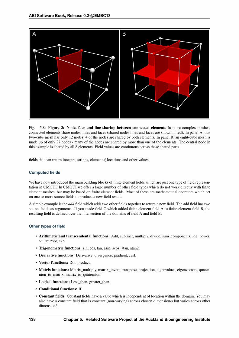
ABI Software Book, Release 0.2-@EMBC13
Fig. 5.8: Figure 3: Node, face and line sharing between connected elements In more complex meshes,connected elements share nodes, lines and faces (shared nodes lines and faces are shown in red). In panel A, thistwo-cube mesh has only 12 nodes; 4 of the nodes are shared by both elements. In panel B, an eight-cube mesh ismade up of only 27 nodes - many of the nodes are shared by more than one of the elements. The central node inthis example is shared by all 8 elements. Field values are continuous across these shared parts.
fields that can return integers, strings, element-𝜉 locations and other values.
Computed fields
We have now introduced the main building blocks of finite element fields which are just one type of field represen-tation in CMGUI. In CMGUI we offer a large number of other field types which do not work directly with finiteelement meshes, but may be based on finite element fields. Most of these are mathematical operators which acton one or more source fields to produce a new field result.
A simple example is the add field which adds two other fields together to return a new field. The add field has twosource fields as arguments. If you made field C which added finite element field A to finite element field B, theresulting field is defined over the intersection of the domains of field A and field B.
Other types of field
• Arithmetic and transcendental functions: Add, subtract, multiply, divide, sum_components, log, power,square root, exp.
• Trigonometric functions: sin, cos, tan, asin, acos, atan, atan2.
• Derivative functions: Derivative, divergence, gradient, curl.
• Vector functions: Dot_product.
• Matrix functions: Matrix_multiply, matrix_invert, transpose, projection, eigenvalues, eigenvectors, quater-nion_to_matrix, matrix_to_quaternion.
• Logical functions: Less_than, greater_than.
• Conditional functions: If.
• Constant fields: Constant fields have a value which is independent of location within the domain. You mayalso have a constant field that is constant (non-varying) across chosen dimension/s but varies across otherdimension/s.
138 Chapter 5. Related Software Project at the Auckland Bioengineering Institute

ABI Software Book, Release 0.2-@EMBC13
• Composite field: Makes a new field built from other fields and field components in any order.
• Image-based fields: These can be used for texture-mapping and image processing. Image processing fieldsusing ITK filters.
• Many more.
These types of fields can be created via gfx define field commands or through the API. Fields are amodular part of the CMGUI application. If a new function is required, it can be added as a field. To get a list ofthe computed fields available in CMGUI, enter gfx define field ?? in the command line.
Fields and visualization
When creating visualizations, you need to choose which field controls which part of a graphics object. Coordinatesin one, two or three dimensions can be used to create spatial representations. Texture coordinate fields can beused to position textures. Orientation or data fields can be used to position glyphs or colour objects such assurfaces. CMGUI allows an enormous amount of flexibility in how fields can be visualized. Further informationon visualizations is available in other documents such as those detailing graphics, glyphs, or surfaces.
5.1.8 Visualizing fields at points using glyphs
Glyphs are graphical objects that are used to represent information at points within a model. These glyphs canbe coloured, scaled, and oriented according to the values of chosen fields. Glyphs might be used for somethingas simple as showing node locations (Figure 1), or something more complex such as showing the strain at pointswithin a deformed mesh. cmgui has a range of glyphs available, for representing different types of point data.This document will explain how to position, scale and orient glyphs in a variety of ways.
Fig. 5.9: Figure 1: Different glyphs placed at the nodes of a cube mesh.
5.1. Cmgui user documentation 139

ABI Software Book, Release 0.2-@EMBC13
Adding glyphs to a mesh
Glyphs are added and edited from within the scene editor. When you select a region in the scene editor, you cancreate a new graphic for placing glyphs at your points of interest. Glyphs can be added at point, node points, datapoints, or element points. Element points are points through the interior of an element at a controllable layout anddensity.
Unscaled glyphs
The simplest use of a glyph is to visually mark a point, with no direction or scale information. Unscaled glyphsare simply glyphs for which you have not selected an orientation/scale field. This means that they simply appearat the points you specify, at the default orientation, and with the specified the base size. The default base size is1*1*1. If you want to run through this example, load up example a1 in cmgui and run the entire com file.
Open the scene editor and make sure cube is selected in the scene object list. You will notice that there are threeitems in the graphics list: lines, node_points, and surfaces. Select the node_points graphics item. You will seein the settings below that these node_points already have glyphs associated with them - in the Glyph drop-downmenu, the glyphs currently used to display the nodes are point glyphs. These are the default glyph, and are bydefault a single white pixel. Figure 2 shows the scene editor window, with the three areas labelled.
Use the drop-down menu to select another type of glyph for the node points: select sphere. In the graphics window,large orange spheres will appear at the corners (node points) of the cube. As the cube in this example is 1*1*1 andthe default size of the glyphs is also 1*1*1, the glyphs will be far too large to be useful. For unscaled glyphs, youcontrol the size by entering your desired size in the Base glyph size text-box, which will currently contain 1*1*1(x*y*z dimensions). Change this to 0.1*0.1*0.1. If you enter a single value in the base glyph size box, it will usethis value for all three dimensions. After changing the glyphs to these dimensions, you will notice that the sphereshave shrunk to a more practical size (Figure 3). For unscaled glyphs, the final size is determined entirely by theBase glyph size.
Final glyph size = b1*b2*b3
This is the most basic use of glyphs - to indicate points such as nodes. Other uses of glyphs allow you to representdata in addition to simple location by using the size, shape, and colour of glyphs.
Scalar glyphs
Scalar glyphs can be used to represent the value of a scalar field at selected points. They have a single componentorientation/scale field, which we will call S. For this case the value of S is used for all three directions of glyphscaling. The size of each glyph dimension (x, y, and z) is determined by the base size (which we will call b) plusthe scale factor (which we will call c) multiplied by the orientation/scale field.
Any scale factors that are given a zero value do not add anything to the base size - in this way it is possible toscale glyphs in one, two, or three dimensions simply by using a zero value for the dimensions along which youdo not wish them to scale. For example, for glyphs that only scale in the z direction, c1, c2, and c3 could be 0, 0,and 0.1 respectively. It can also be useful to set the base size to zero in order that the final glyph size is exactlyproportional to the orientation/scale field.
Vector glyphs
Glyphs used to represent a single vector most often use a three component orientation/scale field, but it is possibleto use a two component field for two-dimensional vectors. The alignment of the glyph is determined by thealignment of the vector defined by the field; the glyph’s first direction aligns to the vector, and its second and thirddirections are arbitrarily aligned orthogonal to this.
The glyph scaling is proportional to the magnitude of the vector, which we will call M. All three directions of theglyph are scaled by this value.
Final glyph size = (b1+c1M)*(b2+c2M)*(b3+c3M)
140 Chapter 5. Related Software Project at the Auckland Bioengineering Institute

ABI Software Book, Release 0.2-@EMBC13
Fig. 5.10: Figure 2: The scene editor.
5.1. Cmgui user documentation 141

ABI Software Book, Release 0.2-@EMBC13
Fig. 5.11: Figure 3: Changing the glyph and its base size.
142 Chapter 5. Related Software Project at the Auckland Bioengineering Institute

ABI Software Book, Release 0.2-@EMBC13
Fig. 5.12: Figure 4: How glyphs are scaled by a scalar orientation/scale field.
In most cases, b1 (base size one) is set to zero so that the final length of the glyphs is directly proportional to M;that is, their size in direction one is entirely determined by the scaling factor c1 multiplied by the magnitude M.Likewise, c2 and c3 can be set to zero so that the width and height of the glyphs are constant; in this case b2 andb3 would be set to the desired constant sizes in these directions.
Two vector glyphs
These are rarely used. They have either four (2D vectors) or six (3D vectors) component orientation/scale fields.Vector 1 is defined by the first 2 or 3 components, and vector 2 by the second 2 or 3 components. The glyphswill orient their first direction along vector 1, and their second direction along vector 2. The glyph’s direction 3direction 3 is equal to the cross product of vectors 1 and 2.
The glyph scaling is proportional to the magnitude of vector 1 (M1) in direction 1, the magnitude of vector 2 (M2)in direction 2, and the cross product of vectors 1 and 2 in direction 3. For two 2D vectors, cmgui assumes a zvalue of 0 in order to obtain the cross product.
M1 = magnitude of vector 1 M2 = magnitude of vector 2 M3 = magnitude of cross product of vectors 1 and 2
Final glyph size = (b1+c1M1)*(b2+c2M2)*(b3+c3M3)
Three vector glyphs
Three vector glyphs use a nine component orientation/scale field: vector 1 is defined by components 1,2,3, vector2 by components 4,5,6, and vector 3 by components 7,8,9. The glyph is oriented in directions 1, 2, and 3 by thedirections of vectors 1, 2, and 3 respectively. The scaling along the three directions is determined by the magnitudeof the three vectors.
Final glyph size = (b1+c1M1)*(b2+c2M2)*(b3+c3M3)
Using the fibre field
A special case of three vector glyphs is when you choose a fibre field for the scale/orientation field. This optionautomatically creates a three vector “fibre axes” field from it together with the coordinate field used by that graphic.This is equivalent to defining a field using the command gfx define field NAME fibre_axes
5.1. Cmgui user documentation 143

ABI Software Book, Release 0.2-@EMBC13
Variable scale glyphs
Variable scale glyphs use an extra “signed scale” field to give a signed magnitude; this not only multiplies themagnitude of the orientation_scale field (so it is doubly-scaled) but its magnitude provides its “sense”. A goodexample of this would be extension (positive) versus compression (negative) for strain. Negative values of thevariable scale field reverse glyphs about their origin along their orientation. The glyph ‘Repeat mode’ allowsglyphs to be mirrored which is useful with line, cone and arrow glyphs to help visualise principal stain and stressfields.
Fig. 5.13: Figure 5: Mirror glyphs and glyph reversal using the variable scale field. A) Mirror-cone glyphsbeing used in the large strain example, with the magnitude and sign of strain indicated by the length and directionof the glyphs respectively. B) How glyphs are represented with differently signed variable scale fields. Un-mirrored glyphs are not as useful for representing this information.
Variable scale glyphs need both:
• direction: orientation_scale field
• magnitude: variable_scale field
The variable scale field is an extra scaling factor in addition to the magnitude of the vector. For the final glyph sizeequation I will call the variable scale field “lambda” - this is because the variable scale field is often the eigenvalueof an eignevector calculated from deformations. Run through the large_strain example (a/large_strain) to see thisin action.
Final glyph size = (b1+c1M*lambda1)*(b2+c2M*lambda2)*(b3+c3M*lambda3)
It is most common to use a variable scale field with single vector glyphs, such as in the large strain example.
Additional tricks with glyphs
Adjusting the glyph offset
All glyphs have a default origin; this is the point which is positioned at the chosen point within the graphicalrepresentation. This can be edited by entering values in the offset value box in the settings editor. This appearsnext to the glyph drop-down menu.
By default, glyphs have a 0,0,0 coordinate point (origin) that is logically positioned according to the purpose ofthe glyph. For directional glyphs, the “long axis” is always the x axis. Spheres, cubes and cylinders have theirorigin positioned in the spatial centre of a bounding unit cube. Directional glyphs such as arrows have their originat the base of the arrow, and axis glyphs have their origin at the intersection of the axes.
Using the offset value box, you can adjust the position of your selected glyph.
144 Chapter 5. Related Software Project at the Auckland Bioengineering Institute

ABI Software Book, Release 0.2-@EMBC13
Fig. 5.14: Figure 6: Origins of various glyph types within their bounding cubes. Origin of each glyph familyis indicated by a red dot.
Using custom glyphs
It is possible in cmgui to create your own glyphs from obj model files. An example of this in action is the biplaneexample, where a model of a biplane is used to create a custom glyph.
5.1.9 Graphics in CMGUI
General description of graphics
graphics are the building blocks used to create any visualization displayed in the CMGUI graphics window. Theyare created, edited, re-ordered and deleted from within the scene editor, or via the command line. Most graphicshave the following settings in common:
• Name: This allows you to set the name of the graphic.
• Coordinate System: This setting can be used to render the graphic according to a range of different coordi-nate systems. This is useful for creating “static” overlays of data on visualizations.
• Coordinate field: This setting has a drop-down menu showing a list of fields that can be selected as thecoordinate field for the selected graphic.
• Tessellation: Tessellation settings are used to set the level of detail of an object. This replaces the discretiza-tion settings from old versions of cmgui.
Note: The only graphics which do not have a tessellation setting are node points, data points, and point.
• Select mode: This drop-down menu allows you to select different selection behaviours for the graphic:
– select_on - The default setting; graphics are able to be selected and selected items are highlighted byrendering in the default_selected material.
– no_select - No selection or highlighting of the graphic.
– draw_selected - only selected items are drawn.
– draw_unselected - only unselected items are drawn.
• Material: This drop-down menu allows you to select which material should be used to render the graphic.Materials are defined and edited in the material editor window.
• Data: This setting has a drop-down menu, allowing you to select which field will be mapped on to thegraphic. This enables you to colour the graphic according to the values of some field, for example. Thecheck box also activates the spectrum drop-down menu.
5.1. Cmgui user documentation 145

ABI Software Book, Release 0.2-@EMBC13
• Spectrum: This drop-down menu is used to select which spectrum is to be used to colour the graphicalelement according to the field selected in the data setting. Spectra are edited in the spectrum-editor-window.
• Selected material: This drop-down menu allows you to set which material will be used to render parts ofthe graphic which are selected.
The eight types of graphics
• node_points
Node points are used to visualize nodes. You can use glyphs to represent node points. There are a range ofbuilt-in glyphs in CMGUI, and it is possible to create custom glyphs as well. Node points graphics have thefollowing settings in addition to the common ones listed above:
– Glyph: this drop-down menu allows you to choose the glyph that will be rendered at the node points.
– Offset: this box allows you to offset the origin of the glyph in order to alter its placement with respectto the node point.
– Base glyph size: This box allows you to enter a size (x,y,z) for the glyph in the same scale as thecoordinate system for the region.
– Orientation/Scale: This check box enables a drop-down menu that allows selection of the field that theglyphs will be oriented and scaled according to.
– Scale factors: This box allows you to enter how each dimension scales according to the orienta-tion/scale field value.
– Variable scale: This check box enables a drop-down menu that allows selection of the field that actsas the variable scale field. For more information on this and other of the node points options, see thedocument on working with glyphs.
– Label: use this drop-down menu allows you to add field-value labels to the glyphs.
• data_points
Data points are used to visualize data points. Like node points, they can be represented using glyphs. Theyhave the same settings as node points.
• lines
Lines are used to visualize 1D elements, or the edges of 2D or 3D elements. They are simple, unshadedlines that have a fixed, specified width. They have the following specific settings:
– Exterior: This check box will automatically only render lines on exterior surfaces of a mesh.
– Face: This check box enables a drop-down menu that allows you to choose which faces are drawnaccording to xi values. You can select xi=0 or 1 for each of the three xi-directions.
– Width: this allows you to specify the width of the lines in pixels. This is a constant width that doesnot scale according to the zoom level.
• cylinders
Cylinders are used to visualize the same things as lines. They are shaded cylinders of a specified radius.They have the following specific settings:
– Exterior: This check box will automatically only render lines on exterior surfaces of a mesh.
– Face: This check box enables a drop-down menu that allows you to choose which faces are drawnaccording to xi values. You can select xi=0 or 1 for each of the three xi-axes.
– Constant radius: This allows you to set the radius of the cylinders, in the units of the coordinate system.
– Scalar radius: This check box will activate a drop-down menu allowing you to select which field willbe used to scale the radius of the cylinders. It will also activate a text box in which you can enter thescale factor, or how the scale field will scale the radius.
– Circle discretization: This sets the number of sides used to render the cylinders in the 3D window.
146 Chapter 5. Related Software Project at the Auckland Bioengineering Institute

ABI Software Book, Release 0.2-@EMBC13
– Texture coordinates: This drop-down menu allows you to select which field will be used to positionany textures applied by the material setting.
• surfaces
Surfaces are used to visualize 2D elements or the faces of 3D elements. They are shaded surfaces of zerothickness that are automatically shaped according to the nodes defining the element they represent. Theirlevel of detail is specified per surface by choosing a tessellation object. They have the following specificsettings:
– Exterior: This check box will automatically only render surfaces on exterior surfaces of a mesh.
– Face: This check box enables a drop-down menu that allows you to choose which faces are drawnaccording to xi values. You can select xi=0 or 1 for each of the three xi-axes.
– Render type: This drop down menu allows you to select shaded (default) or wireframe renderingof surfaces. Wireframe rendering renders the surfaces as grids of shaded lines, with the grid detaildetermined by the tessellation setting.
– Texture coordinates: This drop-down menu allows you to select which field will be used to positionany textures applied by the material setting.
• iso_surfaces
Iso-surfaces are used to represent a surface that connects all points that share some common value. Forexample, in example a7 an iso-surface is used to represent a surface at which every point has a temperatureof 100 degrees C. They have the following specific settings:
– Use element type: This drop down menu allows you to select which type of element will have surfacesrendered on it. Type use_elements is the default. The types use_faces and use_lines will render elementpoints only on those components of elements. If faces or lines are chosen, the following options areactivated:
* Exterior: This check box will automatically only render iso-surfaces on exterior surfaces of amesh.
* Face: This check box enables a drop-down menu that allows you to choose on which faces iso-surfaces are drawn, according to xi values. You can select xi=0 or 1 for each of the three xi-axes.
It is worth noting that if you select use_surfaces then the equivalent of iso-surfaces becomes iso-lines. Ifyou select use_lines then you will not get any visual representation.
– Iso-scalar: This drop down menu allows you to select the field that the iso-surface will be renderedaccording to the values of.
– Iso-values: This settings box contains the following settings:
* List: This radio button activates a text box that allows you to enter a value at which to draw theiso-surface.
* Sequence: This radio button activates three text boxes that allow you to enter a sequence of evenlyspaced values to draw iso-surfaces at. The Number box allows you to enter the number of iso-surfaces you want. The First and Last boxes allow you to enter the starting and ending valuesof the iso-surfaces. The sequence will automatically space the number of surfaces between thesetwo values.
– Render type: This drop down menu allows you to select shaded (default) or wireframe renderingof surfaces. Wireframe rendering renders the surfaces as grids of shaded lines, with the grid detaildetermined by the chosen tessellation object.
– Texture coordinates: This drop-down menu allows you to select which field will be used to positionany textures applied by the material setting.
• element_points
Element points are used to visualize the discretized points within an element. Elements may be 1, 2 or 3dimensional, in which case the element points are spaced along the line, across the surface, or throughoutthe volume according to the chosen tessellation object . They have the following specific settings:
5.1. Cmgui user documentation 147

ABI Software Book, Release 0.2-@EMBC13
– Use element type: This drop down menu allows you to select which type of element will have elementpoints rendered on/in it. Type use_elements is the default, and renders element points throughout 3Delements. The types use_faces and use_lines will render element points only on those components ofelements. If faces or lines are chosen, the following options are activated:
* Exterior: This check box will automatically only render element points on exterior surfaces of amesh.
* Face: This check box enables a drop-down menu that allows you to choose on which faces elementpoints are drawn according to xi values. You can select xi=0 or 1 for each of the three xi-axes.
– Xi discretization mode: this drop down menu allows you to select the method by which element pointsare distributed across the element.
–
• streamlines
Streamlines are a special graphic for visualizing vector fields - for example, a fluid flow solution. Theycan be used to visualize 3, 6 or 9 component vector fields within a 3 dimensional element. In example ao,streamlines are used to show the fibre and sheet directions in the heart. Streamlines will align along theirlength according to the first vector of a vector field, and across their “width” (eg the width of the ribbon orrectangle streamline types) to the second vector. For single vector (3 component) vector fields, the width ofthe streamlines will align to the curl of the vector.
Note that streamlines can be quite expensive to compute; changes to streamline settings in the scene editorcan take several seconds to appear in the 3D window, especially for complex scenes.
Streamlines have the following specific settings:
– Streamline type: This drop-down box allows you to select the shape of the streamlines; that is, theshape outline that is extruded along the length of the streamline. Line and Cylinder can be usedto visualize streamlines without showing orientation (curl). Ellipse, rectangle and ribbon types willenable visualization of the direction of the vector orthogonal to the streamline direction.
– Length: Enter a value into this box to set the length of the streamline/s.
– Width: Enter a value into this box to set the width of the streamline/s.
– Stream vector: This drop-down box allows you to select the vector that is being visualized by thestreamlines.
– Seed element: This setting has a check box which when ticked allows you to specify a single elementto seed a streamline from.
– Xi discretization mode: This drop-down box allows you to set the point in xi-space from which stream-lines are seeded. The setting of exact_xi for example will always seed the streamline at the exact centreof the element’s xi-space.
– Reverse: Checking this box reverses the streamline.
– Seed element: Checking this box allows you to select the single element number from which thestreamline will be seeded.
– Xi: Entering three comma-separated values (between 0 and 1) allows you to set the xi location withinelements from which streamlines will be seeded.
• point
Point graphics are used to add a single glyph to the scene. This is the graphical setting that is used to replacethe old axis creation, for example.
5.1.10 CMGUI Graphics Window
The graphics window is where all visualizations set up in the scene editor window are displayed. It also has toolswhich allow some interactive manipulation of the data being visualized. The window consists of a control panelon the left hand side, and the display area on the left. At the top of the control panel area are a selection of general
148 Chapter 5. Related Software Project at the Auckland Bioengineering Institute

ABI Software Book, Release 0.2-@EMBC13
controls under the “Options” label: view all, save as, and perspective. The view all button will zoom out theviewing area so that all the graphics are visible. The save as option provides the ability to save the viewing areaas a raster graphic, such as a png or jpg file. The perspective check box switches convergence on or off in the 3Ddisplay.
Immediately underneath the options section are controls for selecting how the 3D display is configured. TheLayout drop down list contains a list of display layouts, such as orthogonal or pseudo-3D views. If an applicablelayout is selected, the up and front controls will become available in order to change the viewpoint. Many ofthese layouts contain multiple scene viewers, which may be useful in specific situations. The default layout simpleconsists of a single 3D scene viewer.
Below the layout section is a button labelled “Time Editor”. This opens the timeline controls (much like thecontrols in a media player) that allow you to play animations if they have been set up.
Below this are the 5 “Tools” buttons. These offer different ways of interacting with the 3D display.
The graphics window tools
• Transformation mode
This is the default mode, and is used for simple viewing of the graphical representations you are workingon. In this mode the objects in the 3D window can be rotated, translated and zoomed using the mouse.Holding the left mouse button within the 3D view and moving it around will rotate, or tumble the view.Holding down the right mouse button and moving the mouse up and down will zoom the view in and out,and holding the middle button will allow you to translate the view around along two axes. It is useful tospend some time getting used to the way these manipulations work.
In CMGUI, the rotate function works slightly differently from how similar view manipulations work in mostsoftware. This may not be immediately obvious, as the function does not “feel” particularly different in use;nevertheless there are some useful features of CMGUI’s particular technique for rotating the view.
Essentially, where you initially click in the view is the “handle” that you then move around by moving themouse. In CMGUI this handle is different to most applications, in that it is like “grabbing” a point on asphere that bounds the object in the 3D window. This allows manipulations using the rotate function thatare not possible in most 3D views, such as rotating the object around an arbitrary axis, or rotating it in acircular fashion around the centre of the view. These abilities can be useful when looking at data that hasaligned features.
The four other tools available are used for the selection and limited editing of the type of item they refer to.Selected items are able to be targeted by commands input to the command line, or edited from within thegraphics window.
When any of the following four tools is selected, holding down the Ctrl key will temporarily switch youback into transformation mode in order to manipulate the view.
• Node Tool
The node tool allows the selection and editing of individual nodes from within the graphics window. Se-lected nodes will turn red by default - the selected colour of a node is editable via the scene editor window.There are a range of other options to allow the editing, (moving nodes within the scene viewer) deletion, orcreation of nodes. It is also possible to create 1D, 2D or even 3D (lines, surfaces and volumes) elementsusing the node tool; this functionality is somewhat experimental and is of limited use in most cases.
NOTE: It is somewhat easier to edit nodes (or indeed any of the other editable items) when they are repre-sented by an easily clickable glyph such as a sphere or cube, rather than a point.
• Data Tool
The data tool allows you to select data points and edit them in the same ways that nodes are editable, withthe exception of element creation/destruction which is only available in the node tool.
• Element Tool
The element tool allows you to select and destroy elements. You can also set up filters that allow only theselection of line, face or volume elements. It is worth noting that volume elements have no indication of
5.1. Cmgui user documentation 149

ABI Software Book, Release 0.2-@EMBC13
their selection unless they contain element points, which will turn red when the volume element they existin is selected.
• Element Point Tool
The element point tool allows the selection of element points within the scene viewer/s.
All of the tools that allow selection are useful for creating groups via the command line. You can add selecteditems to a group using the commands
5.1.11 Visualizing element fields using lines and cylinders
Lines and cylinders are graphical representations which can be used to visualize 1-D elements in CMGUI - in-cluding line elements at the edges of 2-D faces or 3-D elements. From Cmgui v3.0, cylinders are just a variantof lines specified by changing the Line shape to ‘circle extrusion’ combined with line scaling options; in previousversions of Cmgui, cylinders were a separate graphics type.
In general, lines are used to visualize the basic shape of a mesh. Note in very old versions of Cmgui lines wereautomatically created when region ‘groups’ were read from file, but this is no longer the case: all graphics mustbe intentionally created by the user (see the scene editor).
If you wish to create lines in the graphics window, you first need to read a model containing line elements. Asan example go to the file menu in CMGUI and select Read, then Node file. Read in cube.exnode from theexample a2 directory. Then using the Read and Elements file menu options, read in cube.exelem from thesame directory. Select the Graphics Scene Editor menu item and select the region you wish to create graphics forfrom the list at the left; in the example it is the root region “/”. Click on add and select lines. A default coordinatefield will automatically be chosen, which is the minimum needed for lines graphics. If you now create a graphicswindow (using the Graphics menu item 3-D window) you will see this cube rendered in 1 pixel thick lines usingthe default (white) material.
Fig. 5.15: Figure 1: The lines graphics created for a cube mesh. This mesh was created by reading thecube.exnode and cube.exelem files from example a2. Note that the example a2 com file creates cylindersto visualize the cube mesh.
150 Chapter 5. Related Software Project at the Auckland Bioengineering Institute

ABI Software Book, Release 0.2-@EMBC13
Settings for lines
The tessellation option in the scene editor controls the number of line segments used along the line element toapproximate a curve or control visualisation of the data field along it. With ‘circle extrusion’ line shape (cylinders)the Circle Divisions option on the tessellation controls the number of line segments around the cylinder with highernumbers better approximating a circle. (Prior to Cmgui v3.0 Cylinder graphics had a Circle discretization valuefor this purpose.) (Figure 2).
Lines have relatively few settings for altering their appearance (Figure 2). The following settings are available forlines:
• Coordinate field: When you check this box, you are able to select the coordinate field that the lines aredrawn according to. This is used any time the coordinate field used for the lines needs to differ from thedefault coordinate field used for the whole graphical element (in the general settings).
• Exterior: When this check box is selected, the lines will only be drawn on the exterior faces of a 3D mesh,or the outside edges of a 2D mesh. This can be useful with large, complex meshes.
• Face: Checking this box allows you to select which face of 3D elements is visualized by lines. Faces areselected according to one of the 3 xi directions of the element, and it’s value (either 0 or 1).
• Select mode: This drop-down menu allows you to select different selection behaviours for the lines.
– select_on - The default setting; line elements are able to be selected and selected elements are high-lighted by rendering in the selected material.
– no_select - No selection or highlighting of line elements.
– draw_selected - only selected lines are drawn.
– draw_unselected - only unselected lines are drawn.
• Material: This drop down menu allows you to select which material the lines will be rendered as. Materialsare defined in the material editor window. Note: the material for lines is unshaded. This means that linesonly use the diffuse colour for the selected material to draw the lines.
• Line width: You can enter a value in this box to set the thickness of the lines in pixels. This width isindependent of zoom, and remains constant through any transformation. Setting this value to 0 results inlines of 1 pixel wide (the default).
• Data: This setting allows you to choose a field which is used to colour the lines according to a spectrum.Use the Spectrum drop-down menu to choose from one of the spectra defined in the spectrum editor window.
• Selected material: Use this drop-down menu to select which material will be used to render selected lines.
In addition to these settings there is a command line setting that can be very useful when using line based visu-alizations: gfx modify window 1 set perturb_lines. This command helps to prevent the “dottedlines” effect that occurs when lines and surfaces interfere.
Note: if no lines appear, you may not have added faces (and lines) to the mesh - try the gfx define facescommand.
Settings for cylinders
Since Cmgui v3.0 cylinders are just lines using additional ‘line shape’ options shared with streamlines graphics,currently restricted to ‘line’ or ‘circle extrusion’ with equal scaling in all lateral directions. Note when choosing aline shape other than the default ‘line’, the resulting graphics scale with the model as you zoom in, whereas ‘line’shape gives constant thickness in screen space.
Options controlling the visualisation with ‘circle extrusion’ line shape:
• Line base size: This is the base diameter of the cylinders in units of the current graphics coordinate system;scaling by field with scale factors is added to this value. It currently has 2 values which are constrained tobe equal, anticipating future use. Beware that prior to Cmgui v3.0 the equivalent option was the ‘Constantradius’.
5.1. Cmgui user documentation 151
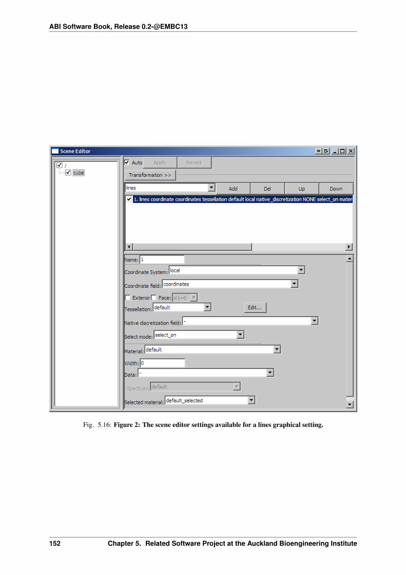
ABI Software Book, Release 0.2-@EMBC13
Fig. 5.16: Figure 2: The scene editor settings available for a lines graphical setting.
152 Chapter 5. Related Software Project at the Auckland Bioengineering Institute

ABI Software Book, Release 0.2-@EMBC13
• Line scale field: This drop-down menu allows you to select a scalar field to scale the diameter of thecylinders across the model according to this field. A good example of this is shown in example a4. Bewarethat prior to Cmgui v3.0 the equivalent option was the ‘scalar radius’ field’.
• Line scale factors This box allows you to enter two values as factors for the scaling the ‘line scale field’lateral to the line, but note that they are currently restricted to being equal-valued. (In future, differentscaling in each lateral direction is anticipated, for use with multi-component ‘line scale fields’). Important:use a value of “2*2” if the line scale field is a radius.
5.1.12 CMGUI Material Editor Window
The material editor window is where you define materials to be applied to graphical elements or objects in thegraphics window. Along the top of the material editor window are three buttons; create, delete and rename. Youcan create a new material, delete or rename an existing material using these buttons. Below these buttons is thelist of currently defined materials. These will contain the default materials, as well as any defined in any comfilethat has been run.
Below the material list is a panel containing four colour editors. These control the ambient, diffuse, emitted andspecular colours.
• Ambient - The ambient colour is the “unlit” colour, or the colour of parts of the object that are in shadow.
• Diffuse - This is the overall colour of the material, the colour that the lit parts of the object will appear.
• Emitted - The emitted colour is the “glow” of a material; this colour will appear in both the lit and unlitparts of the material.
• Specular - This is the colour of the shine that appears on the material. This shine appears as a glossyhighlight.
Each colour can be edited using three sliders or textboxes, and you can choose from three colourspaces for editingthe colour. The default is RGB, but the HSV and CMY colourspaces are also available from a drop-down menuat the top of each colour editor. Each colour editor has a preview panel showing a flat sample of the colour that isbeing edited.
Below the colour editors is the surface editor. This panel allows you to set the alpha, shininess, and textureproperties of the surface of the material being edited. The alpha value sets the transparency of the material. Theshininess sets the “tightness” or size of the specular highlights of a material; generally the higher the shininess,the smaller and harder-edged the highlights. Higher shininess makes a material look glossier. The surface editoralso allows you to assign a texture to the material surface - this option is unavailable unless you have created atleast one texture by using the gfx create texture command to read in some bitmapped graphics. Thereare two other check box options available in the surface editor: “per pixel shading” which greatly increases thequality of the lighting of the material, and bump mapping which allows you to use a texture file to create surfacedetails. These options are only available on hardware that supports advanced forms of shading.
Below the surface editor is a panel that shows a preview of the currently edited material applied to a sphere. Youmay need to resize the material editor window in order to see a usefully large preview panel. Clicking in thepreview panel will cycle the background from the RGB colours through black, white and back to RGB.
At the bottom of the window are four buttons: OK, apply, revert and cancel. The OK button leaves the editor andapplies the changes made. The apply button immediately applies current changes to the materials, allowing youto see how they look if they are used in any objects shown in the graphics window. The revert button will undoany changes made to the currently edited material, and the cancel button exits the material editor window withoutapplying changes.
5.1.13 CMGUI Scene Editor Window
The scene editor is used to control how visualizations appear in the graphics window. From this window you can:
• Toggle visibility for any part of the region tree.
• Toggle visibility of any individual graphics setting for a region.
5.1. Cmgui user documentation 153

ABI Software Book, Release 0.2-@EMBC13
Fig. 5.17: Figure 1: The CMGUI Material Editor
154 Chapter 5. Related Software Project at the Auckland Bioengineering Institute

ABI Software Book, Release 0.2-@EMBC13
• Add, remove, and edit graphics.
• Alter the order in which graphics are drawn.
The window itself is broken into four main areas; region tree, transformation controls, graphics list, and settingseditor (Figure 1).
Fig. 5.18: Figure 1: The scene editor.
Region tree
At the left hand side of the Scene Editor window is the region tree, where all regions are listed. Each regionhas a visibility toggle, controlled by clicking on the box alongside its name. All ticked regions will be visible inthe graphics window, provided that they have some visible graphics. Regions may contain sub-regions, allowingpowerful control over visibility of the parts of a complex model.
Alongside the region tree are the transformation settings, graphics list, and settings editor. These are used tocontrol and edit the visualisations of the currently selected region in the region tree.
Note: Previous versions of cmgui also had a “General Settings” section in this window, which was used to set
5.1. Cmgui user documentation 155

ABI Software Book, Release 0.2-@EMBC13
the level of detail (discretization) of objects. This system has been replaced by the new tessellation object. Youare now able to use different levels of detail for different graphics, allowing you to choose the most appropriatefor each. This also allows you to change the detail levels of a number of graphics by simply altering a singletessellation object that has been applied to them all. The tessellation is set for each graphical setting using thesettings editor.
Graphics list
Below the transformation and general settings buttons is the graphics list. This is where the visual representationsof the currently selected region are listed. This panel allows creation, deletion, visibility switching (on or off) andre-ordering of these visual representations.
Settings editor
Below the graphics list is the settings editor where each graphical setting can be edited. When a graphical settingis selected from the list, all of its editable properties appear in this area. The range of editable properties will varydepending on the type of graphics currently selected.
5.1.14 CMGUI Spectrum Editor Window
The spectrum editor window is where you define spectra to be applied to graphical elements or objects in thegraphics window. Spectra are used to visualize continuous data ranges within models using colour ranges, andcan be applied to the graphics that have been used to create your visualization. The window is divided into threebasic areas; the spectrum list, the preview panel, and the settings editor (Figure 1).
It is useful to step through example a7 to get a feel for the use of spectra in cmgui. This example uses a meshcontaining a number of fields that can be usefully visualized using spectra.
Spectrum List
The spectrum list shows all the currently defined spectra; it will always contain the default spectrum if no othershave been defined. Three buttons at the top of the window allow you to create, delete, or rename spectra. Justbelow the list of spectra are some controls that allow you to set some of the general properties of the selectedspectrum. The autorange button automatically sets the minimum and maximum values of the selected spectrum,according to the smallest and largest values it has been applied to in the scene editor. For example, if the defaultspectrum has been used to colour a temperature field in the default scene, and that field has values ranging from 0to 100 degrees Celsius, pressing the autorange button will set the minimum and maximum values (in the Spectrumrange settings - see below) of the selected spectrum to 0 and 100 respectively. If the selected spectrum has beenused to colour objects according to more than one field, the autorange function will choose the smallest and largestvalues across all of these fields. The from scene drop-down menu allows you to select the scene from which thespectrum will be auto-ranged.
The overlay or overwrite options allow you to choose whether a spectrum will completely over-ride any othermaterial settings (overwrite), therefore completely colouring the object as the spectrum appears in the previewpanel - or whether the spectrum combines with the other material settings of the object so that the final colour is acombination of the spectrum and other material settings (overlay).
Preview Panel
This panel shows a horizontal bar, coloured using the selected spectrum. The bar also shows the range that thespectrum is currently set to, using a series of numbered labels. Clicking in the preview panel changes the numberof these labels from 4 to 10 to 2, then cycles through these values. Currently the preview panel can not displaymulti-component spectra.
156 Chapter 5. Related Software Project at the Auckland Bioengineering Institute

ABI Software Book, Release 0.2-@EMBC13
Fig. 5.19: Figure 1: The spectrum editor.5.1. Cmgui user documentation 157

ABI Software Book, Release 0.2-@EMBC13
Settings Editor
The settings editor is where each spectrum is set up. It contains a number of controls.
• Spectrum component list: The top of this list has four buttons; Add, Delete, Up, and Down. Below thesebuttons is a list of the components that make up the selected spectrum. Spectra in cmgui can be made upof multiple components; these can be added, deleted or re-ordered using this list. Using these “sub-spectra”you are able to create spectra that have different colour ranges for different parts of the data range theycover, or spectra that have different colour ranges for different dimensions.
• Data component: This text box allows you to enter which data component of a multi-component field thespectrum will colour according to.
• Spectrum range: This set of controls is used to set up the range of values the spectrum covers. The Min.and Max. text boxes allow you to enter values for the minimum and maximum values of the spectrum.There are also four check boxes that allow you to change the behaviour of a spectrum at its start and endpoints.
• Colour: This drop-down menu provides a selection of pre-set colour settings that can be applied to thecurrently selected spectrum component. Although many of the colour ranges are fairly self-explanatory, anumber of them have special features which are useful for creating specialized spectra. The contour bandsand step colour settings have further settings associated with them.
– Rainbow: This is a standard rainbow colour range.
– Red: This is a red to black colour range. It is applied as a single “channel” of red to the spectrum; thiscan be used to add to other spectrum components to make multi-component spectra.
– Green: This is a single channel green to black colour range.
– Blue: This is a single channel blue to black colour range.
– White to blue: This is a white to blue colour range.
– White to red: This is a white to red colour range.
– Monochrome: This is a black to white colour range.
– Alpha: This is a single channel transparent to opaque spectrum.
– Contour bands: This colour option creates a series of evenly spaced black bands that can be furtheredited to get the correct number, width and spacing desired.
– Step: This is a colour range which has a sharp transition from saturated red to saturated green.
• Type: This drop down menu allows you to choose between linear and log scale spectra. The Reverse checkbox allows you to swap the direction of the spectrum. If a log scale is selected as the type, the Exaggerationsettings become available.
– Exaggeration: This text box allows you to specify how strongly the spectrum is exaggerated.
– Left/Right: These radio buttons allow you to choose the direction of the exaggeration.
• Normalised colour range: These two text boxes allow you to specify the portion of the colour range thatis displayed across the chosen range of values for the spectrum component. The default values of 0 and 1display the entire colour range, and other values allow you to choose where in the colour range the spectrumcomponent begins and ends. For example, 0.5 and 1 would display only the upper half of the colour range;0 and 0.5 would display only the lower half; 0.25 and 0.75 would display the middle section of the colourrange.
• Number of bands: This text box is enabled when the contour bands colour type is chosen. Enter a valueto specify the number of contour bands.
• Step value: This text box is enabled when the step colour type is chosen. Enter a value somewhere betweenthe values specified in Spectrum range to specify where the step occurs in the spectrum.
158 Chapter 5. Related Software Project at the Auckland Bioengineering Institute
ABI Software Book, Release 0.2-@EMBC13
5.1.15 Visualizing element fields using surfaces
Surfaces are graphical representations that can be used to represent two or three dimensional elements in CMGUI.Surfaces can be used to represent the faces of a 3D element or mesh, for example.
Surfaces and are created as graphics in the scene editor. To create a very simple surface graphic, go to the Filemenu, select Read, then Node file. Read in cube.exnode from the example a2 directory. Then using the Readand Elements file menu options, read in cube.exelem from the same directory. If you now create a graphicswindow, you will see a simple cube rendered in the default lines graphic. Open the scene editor window byselecting it from the Graphics menu. Select the cube scene object, then in the graphics panel select surfaces in thedrop-down menu. Click the Add button to the right of this menu. A new graphical setting will appear in the list,below the lines graphical setting. In the 3D window, your cube will now be rendered with white shaded surfaces.
The tessellation setting of the surface graphical setting determines the detail level of surfaces. Each face in asurface graphical setting is divided into a number of squares (each made up of two triangles) determined by thetessellation. The discretization can be independently set for each of the three coordinate dimensions, allowing youto set different detail levels for different parts of surface.
5.1.16 Creating an AVI from a series of images - Windows
This tutorial will describe a method of compiling a series of images saved from CMGUI into an AVI format moviefile on the Windows operating system. There are other methods, but the one described here can be achieved easilyusing free software, and produces excellent, highly customizable results.
An AVI file is a Windows format - however, it can be played on most computers including those running Mac OSX or Linux. It can also be uploaded to online video sites such as YouTube.
Software used
The following pieces of software are used in this tutorial - click on the name of the software to navigate to adownload page for each item:
• VirtualDub - This is an open source AVI editing/capturing application. For the purposes of this tutorial, itallows you to load in a series of image files as movie frames, and save the resulting movie as an AVI.
• FFDShow - This is a Video for Windows and Directshow codec for decoding and encoding a large numberof video and audio formats. With this installed you can save AVI files from VirtualDub using a large rangeof codecs.
• WinFF - This is a free windows front-end to ffmpeg (. This tool allows easy conversion of videos from oneformat to another.
• CamStudio - This is a free open source tool for recording screen activity. This represents an alternativemethod for capturing quick movies of CMGUI.
Installation of VirtualDub and FFDShow is a requirement for following this tutorial. You will need administratorrights on your computer to install FFDShow; VirtualDub is simply unzipped into a directory and run directly.Camstudio is only required if you wish to experiment with recording the CMGUI graphics window directly.
Compiling a series of images into a movie
When making a movie from a sequence of images, it is important to make sure that the images you created inCMGUI are saved at a usable resolution. It is always best to use familiar resolutions like 800x600, 1024x768,or 1920x1080. Many video formats require specific resolutions to work properly; codecs often are restricted tomultiples of 2, 4, or 8 for both the height and width in pixels.
Creating a movie from a series of images using VirtualDub is very simple:
• Load VirtualDub. The first time you do this you may be presented with a window where certain optionsmay be set. You can safely dismiss this window and load VirtualDub.
5.1. Cmgui user documentation 159
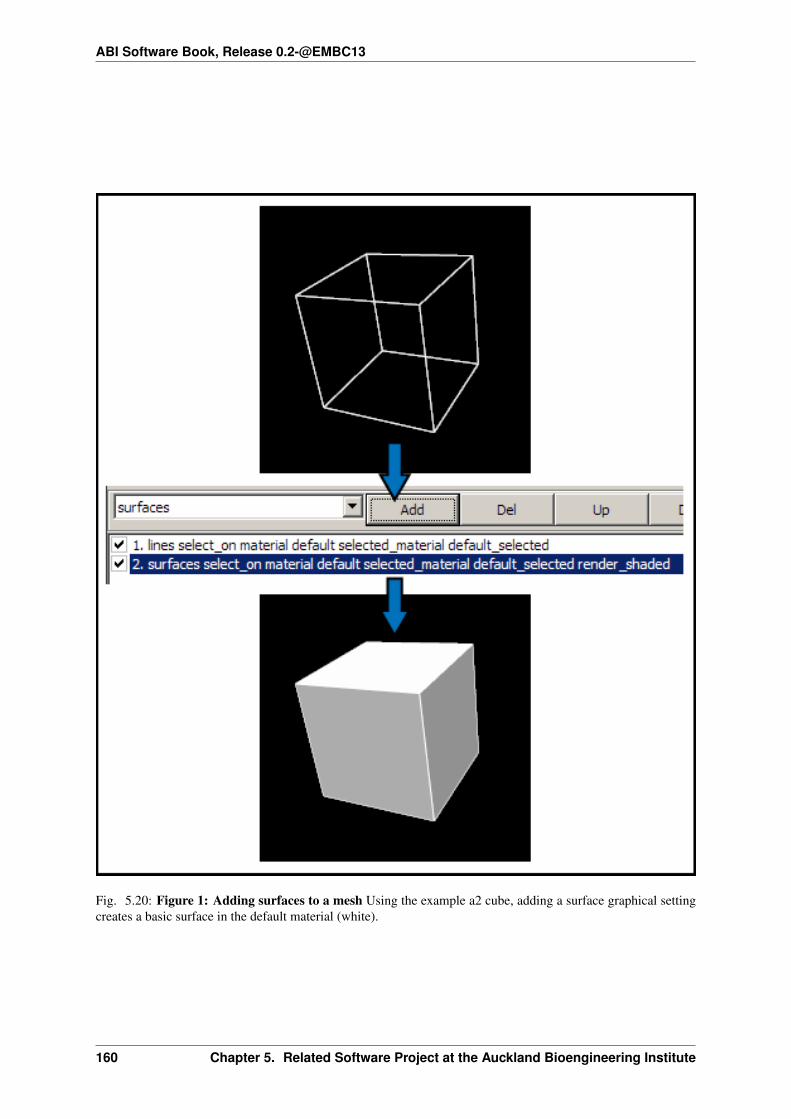
ABI Software Book, Release 0.2-@EMBC13
Fig. 5.20: Figure 1: Adding surfaces to a mesh Using the example a2 cube, adding a surface graphical settingcreates a basic surface in the default material (white).
160 Chapter 5. Related Software Project at the Auckland Bioengineering Institute

ABI Software Book, Release 0.2-@EMBC13
• Go to the File menu and select Open video file.... (Ctrl-O)
• Locate and load the first image in your sequence of images.
VirtualDub will automatically load the entire numbered sequence of images in as movie frames, in the correctorder. This works whether you have a 00001-99999 or a 1-99999 style numbering scheme. You will now see two“screens” side by side, each displaying the first image in your sequence. This is the first frame of your movie,which can now be played within VirtualDub. The two screens display the input and the output. The input screenshows the movie you loaded, in this case the series of frames from the images. The output screen shows theoriginal movie with any filters (such as resizing, contrast adjustments, sharpening etc) that you have applied to it.
Fig. 5.21: Figure 1: The main VirtualDub window This window displays the play controls (which also includemarking tools for editing the video), the input and output panels, and the menus.
The next step is to set up the compression and codec settings of the movie you are going to save.
• Go to the Video menu and select Compression.... (Ctrl-P)
• Select the ffdshow Video Codec from the list of codecs.
• Notice the Format restrictions box on the right hand side - this will inform you of any requirements yourselected codec has for input. For the ffdshow codec, your video resolution must be a multiple of 2 in both
5.1. Cmgui user documentation 161
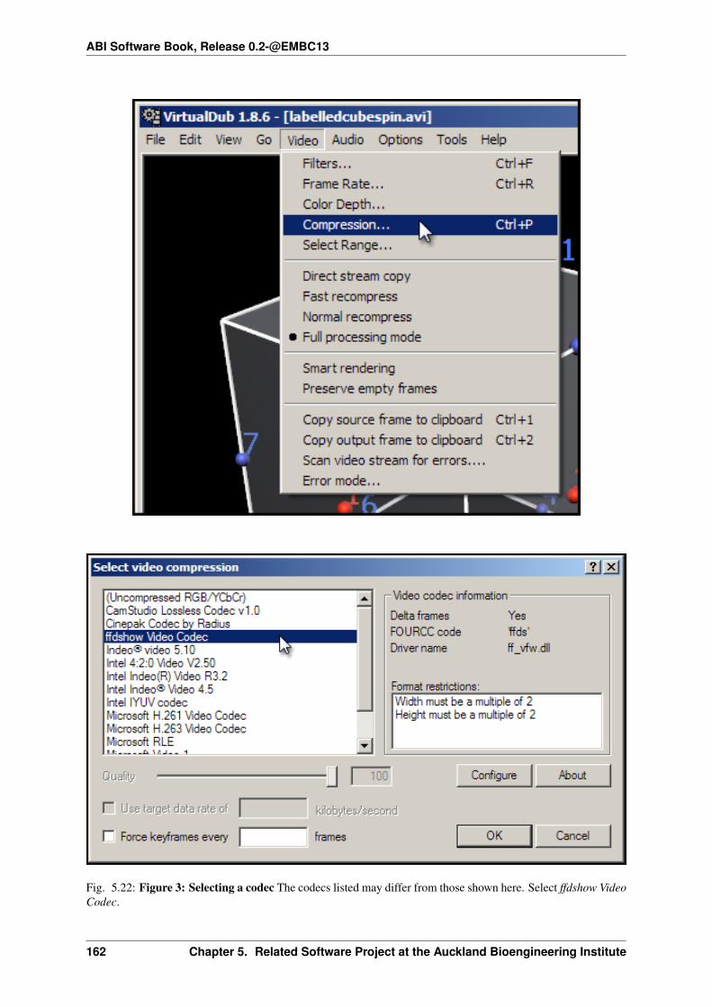
ABI Software Book, Release 0.2-@EMBC13
Fig. 5.22: Figure 3: Selecting a codec The codecs listed may differ from those shown here. Select ffdshow VideoCodec.
162 Chapter 5. Related Software Project at the Auckland Bioengineering Institute

ABI Software Book, Release 0.2-@EMBC13
width and height.
• Click on the Configure button. This will bring up a window with a range of settings for how the codec willbe used to compress your movie.
Fig. 5.23: Figure 4: The codec configuration window This window displays the controls for how the codec willcompress your movie. The ffdshow codec actually enables you to encode your movie in any of a large number ofdifferent codecs; the codec is chosen from the codec selection drop-down menu.
From this settings window you can set up which codec you wish to use to compress your movie, and how muchcompression you wish to apply. Different codecs have different pros and cons; these days it is often best to stick tothe more modern codecs, as a majority of computers on all platforms should be able to play them. Good codecs tochoose are MPEG-2, MPEG4, and H.264. MPEG-2 is an older codec that offers good backwards compatibility, butencodes lower quality videos with larger file sizes. MPEG4 and its successor H.264 generally offer substantiallybetter quality and/or smaller file sizes. The following steps will produce an AVI using the MPEG4 codec, whichis widely supported. If you wish to use another codec, the steps are essentially the same.
• Select the MPEG-4 codec from the codec selection drop-down menu.
• Make sure the Mode setting is one pass - average bitrate.
• Set the Bitrate (kbps) text box to 1000.
• Click Apply and then OK. Click OK in the codec selection window.
• In the main VirtualDub window, go to the File menu and select Save as AVI. Enter a name for your movieand click Save.
5.1. Cmgui user documentation 163

ABI Software Book, Release 0.2-@EMBC13
Fig. 5.24: Figure 5: Progress window
164 Chapter 5. Related Software Project at the Auckland Bioengineering Institute

ABI Software Book, Release 0.2-@EMBC13
A status window will appear, with some information about the progress of the AVI creation.
Once the encoding is finished, find your file and double click on it to play it. Check the file size, and the qualityof the movie. If the file is too big, change the codec settings to use a lower bitrate and save it again. If the movieis poor quality, set the bitrate higher and try again. 1000 kbps gives a good quality 640x480 movie in MPEG-4encoding, with file sizes of about 7 megabytes per minute. With H264 encoding, bitrates as low as 300kbps cangive remarkably good results at 640x480 depending on the content of the movie.
Creating a movie from images using FFMPEG
An alternative to using Virtualdub is to use the command line tool FFMPEG2. This is a powerful, open sourcetool that can perform a large number of video-related tasks. Documentation for FFMPEG can be found on theproject website.
An example command line for creating a movie from image files using FFMPEG is:
ffmpeg -f image2 -i image%d.jpg output.mpg
For more information, please refer to the documentation linked to above.
Converting your movie to other formats
Sometimes you will want to have your movie in a format other than AVI, or you may wish to further tune thecompression and quality of your movie. For example, using the H.264 codec with an AVI creates a non-standardfile; it is usually better to encode an mp4 file using H.264.
Converting to mp4 using Handbrake
Handbrake is an open source video converter that is very fast and effective for converting videos to MP4 format.The application is quite easy to use, and has a number of built-in presets for converting video for certain purposessuch as uploading to youtube, or playing on mobile devices.
Convert your movie to another format using WinFF
WinFF is a useful tool for optimizing the file size or quality of your movies, as well as for converting from AVI toother file formats such as mp4 or mov. When converting using WinFF, it is useful to have an uncompressed moviefile to work with. To create an uncompressed AVI from VirtualDub, select the Uncompressed RGB/YCbCr codecwhen creating the AVI file as detailed above.
The following steps detail how to encode an H.264 codec mp4 file from an AVI:
• Load WinFF.
• Click on the Options button (far right) to show the advanced options.
• Click on the Add button, and select the movie file you wish to convert.
• Select MP4 from the Convert to... drop-down menu.
• Select H.264 in MP4(4:3) from the preset drop-down menu, to the left of the Convert to... drop-down menu.The 4:3 refers to the aspect ratio of your video; standard sizes such as 320x240, 640x480 or 1024x768 havethis aspect ratio. If your movie has a different aspect ratio, enter it into the Aspect Ratio text box, or enterthe resolution of your movie directly into the Video Size text boxes.
• Enter a value such as 500 or 1000 into the Video Bitrate text box.
• Click on the Convert button.
By default, WinFF will create the converted movie file in your My Documents folder. You may choose a differentdesination folder for the converted movie by entering a different path in the Output Folder text box.
5.1. Cmgui user documentation 165

ABI Software Book, Release 0.2-@EMBC13
5.1.17 The cmgui EX format guide: exnode and exelem files
Contents
• The cmgui EX format guide: exnode and exelem files– Overview– General Syntax– Regions– Groups– Field declaration headers– Comments– Defining nodes and node fields– Defining elements and element fields– Further information
Overview
Spatially-varying “finite element” field definitions are commonly imported into cmgui in two parts:
1. ”.exnode” files containing definitions of nodes which are points identified by a unique integer identifier, andfor which field parameters are listed.
2. ”.exelem” files containing definitions of elements which are n-dimensional coordinate spaces, and the func-tions giving field values over them, usually by interpolating node field parameters.
This division is arbitrary since they share a common format able to define both nodes and elements, and the fieldsdefined over them. The extensions ”.exnode” and “exelem” are merely conventions for the above uses. Anyfilename extension is acceptable, and full file names with extensions should always be specified in your scriptsand command files.
Nodes with literal field values stored for them do not just support element interpolation, but are widely used torepresent any point data, and there need not be any associated elements. You will occasionally see files with the”.exdata” extension which are identical to ”.exnode” files but read in with a different command (“gfx read data. . . ”) so that the objects and associated fields are put in a different set of node objects referred to within cmgui asdata rather than nodes, and which are unable to be interpolated in element fields. Note the current limitation ofcmgui that each region consists of one list of node objects, one list of elements, and one list of data points.
General Syntax
Cmgui EX files are human-readable text files which are usually created by export from cm or OpenCMISS. Theycan also be created by scripts or by hand. Due to their complexity, particularly in defining element interpolation,editing an existing file is usually the easiest way to create new data files by hand.
The format has been around for many years and has several exacting rules which can catch the unwary:
1. Main blocks of the file begin with tokens such as “Group name”, “Shape”, “#Fields”, “Node”, “Element”which must be written in full with exact capitalization. Within these blocks are further tokens indicatingsub-blocks of data to be read, each with their own rigid rules.
2. The characters used to separate tokens, identifiers, parameters and other data are quite inconsistent andcould be white space, commas, colons, full stops (periods), equal signs and so on. In each case the precisecharacter must be used. Whitespace separators generally includes any number of spaces, tabs, end of lineand line feed characters. Non-whitespace separator characters can generally be surrounded by whitespace.
3. All array indices start at 1, but scale factor index 0 has the special meaning of using unit scale factor value,1.0.
4. Node and element identifiers must be positive integers.
166 Chapter 5. Related Software Project at the Auckland Bioengineering Institute

ABI Software Book, Release 0.2-@EMBC13
Fortunately, cmgui import commands (“gfx read node/element/data”) report the line number in the file at whichthe first errant text is located (do not confuse this with line element numbers). Unfortunately the actual problemmay be earlier: if the previous block was incomplete then the first text of the next block, however correct, will becomplained about as not matching the tokens and data expected for the previous block.
Regions
The EX format defines fields, nodes, elements and groups (sets of nodes and elements) within regions. Theseobjects belong to their respective region and are independent of similarly identified objects in other regions.
Cmgui version 2.6 (released: May 2009) introduces a “Region” keyword which specifies the path to the regionwhich any following fields and objects are defined within until the next Region keyword or end of file. The formatis as follows:
Region: /PATH_TO_REGION
Examples:
! The root region for this file:Region: /
! Region "joe" within region "bob":Region: /bob/joe
The region path must always be written as an absolute path from the root region of the file, i.e. as a series of zeroor more region names starting with and separated by forward slash “/” characters. Region names must start withan alphanumeric character and contain only alphanumeric characters, underscores ‘_’ and spaces; spaces are notpermitted at the start or end of the name. Colons ‘:’ and dots/periods ‘.’ are permitted but discouraged.
Versions of cmgui prior to 2.6 implicitly read data into the root region, and will report an error for the unrecognised“Region” keyword. The first non-comment keyword in post Cmgui 2.6 EX files should be a Region keyword; tomaintain compatibility with older files it may alternatively begin with a Group declaration.
With EX files you are free to put many regions (and groups) in the same file, or to keep each region (or group)in separate files. The choice is up to the user, although it is more flexible to use separate files, since commandsfor reading EX files into cmgui (e.g. gfx read nodes/elements/data) permit the file’s root region to be mapped toany region. For maximum flexibility and to avoid potential merge conflicts, it is recommended that you keep yourmodel data out of the Cmgui root region.
Cmgui example a/region_io gives several example EX files defining fields in regions and sub-groups.
Groups
The Group keyword indicates that all following nodes and elements until the next Group or Region keyword are“tagged” as belonging to a group (set) of the specified name:
Group name: GROUP_NAME
There can be any number of groups in a single region, each potentially sharing some or all of the same nodes andelements from the region they belong to. Groups are entirely contained within their particular region; groups withthe same name in different regions are completely independent.
Groups have the same name restrictions as regions. They are not written as a path - just a single name within theenclosing region.
Older versions of Cmgui required nodes, elements and fields to always be defined within a group (within theimplied root region), hence the Group keyword was always the first keyword in the file. Since Cmgui 2.6 this isno longer a limitation.
In older EX files it was common to have fields defined after/within a group declaration. However the groupingonly ever applies to nodes and element - fields always belong to the region. It is more common to define the fieldswith nodes and elements under the region with no group, and list only node and element identifiers with no fieldsunder the groups.
5.1. Cmgui user documentation 167

ABI Software Book, Release 0.2-@EMBC13
Field declaration headers
Whether the EX file is listing nodes or elements, there is broad similarity in the way in which they and their fielddata is listed. It consists of a header declaring the number and details of fields being defined for the respectiveobject type, followed by the definitions of the objects themselves. An example header:
#Fields=11) coordinates, coordinate, rectangular cartesian, real, #Components=3... field data specific to nodes or elements ...
The above header declares a field with the name “coordinates”. The field is tagged as usage type “coordinate”- this is a hint which tells cmgui that this field is appropriate for use as a coordinate field. Other values forthis hint are “anatomical” for special fibre fields, and “field” for all other fields. By default, cmgui will use thefirst coordinate field in alphabetical name order for the coordinates of graphics. The coordinates declared in thisheader are embedded in a rectangular Cartesian coordinate system with 3 real-valued components. The rectangularCartesian coordinate system is assumed if none is specified. The value type real is frequently omitted as it is thedefault; other types such as integer, string and element_xi are only usable in node fields and integer for grid-basedelement fields. More complex declarations are given throughout this document. Note that if there is no headeror the header has “#Fields=0”, then nodes and elements can be defined or listed for adding to a group withoutdefining fields.
Following each line declaring the main details of a field are the details on each field component including thename and the parameter values to be supplied with each node, or the basis functions and parameter mappings tobe supplied with each element. These are described later.
There can be only one field of a given name in a region, but it can be defined on nodes, elements and data in thatregion provided the field is consistently declared in the header, including same value type, numbers of componentsand component names.
Note that the #Fields keyword in element field headers are additionally preceded by the following keywords andsub-blocks which are described in later examples:
#Scale factor sets=~...#Nodes=~
Comments
Since Cmgui version 2.6 EX files containing comments are now able to be read. Comment lines begin with !(exclamation mark character) and may only be placed in parts of the file where a Region, Group, Shape, Node,Element, Values or #Field header keyword is permitted. Putting comments anywhere else will result in obscureerrors or undefined behaviour!
Comments are useful for adding source details or copyright/license information to your files, or to document partsof the file. Cmgui ignores the comment lines: they will not be rewritten when exporting an EX file.
Some example comments preceding other keywords:
! Copyright (C) 2009 The AuthorRegion: /heart
! This following node is the apex of the heart:! It has 10 versions of all nodal parametersNode: 13
Note that errors are reported if you attempt to read EX files with comments into versions of Cmgui prior to 2.6.
168 Chapter 5. Related Software Project at the Auckland Bioengineering Institute

ABI Software Book, Release 0.2-@EMBC13
Defining nodes and node fields
Example: specifying 3-D coordinates of nodes
Following is an example reading 8 nodes numbered from 1 to 8, with a field “coordinates” giving positions at thecorners of a unit cube, adapted from cmgui example a/a2:
Region: /cubeShape. Dimension=0#Fields=11) coordinates, coordinate, rectangular cartesian, #Components=3x. Value index=1, #Derivatives=0y. Value index=2, #Derivatives=0z. Value index=3, #Derivatives=0
Node: 10.0 0.0 0.0
Node: 21.0 0.0 0.0
Node: 30.0 1.0 0.0
Node: 41.0 1.0 0.0
Node: 50.0 0.0 1.0
Node: 61.0 0.0 1.0
Node: 70.0 1.0 1.0
Node: 81.0 1.0 1.0
Notes:
• The first line indicates that the following objects will be put in a group called “cube”. Ex files must beginwith a group declaration.
• The second line says that zero dimensional nodes are to be read until a different shape is specified. You willseldom see this line in any .exnode file because 0-D nodes are the default shape at the start of file read andwhen any new group is started.
• The next five lines up to the first Node is a node field header which declares finite element fields andindicates what field parameters will be read in with any nodes defined after the header. The first line of theheader indicates only one field follows.
• The first line following the #Fields declares a 3-component coordinate-type field called “coordinates” whosevalues are to be interpreted in a rectangular Cartesian coordinate system. This field defaults to having realvalues.
• Following the declaration of the field are the details of the components including their names and the pa-rameter values held for each, with the minimum being the value of the field at that node. The above nodefield component definitions indicate that there are no derivative parameters. The “Value index” is redundantsince the index of where values for components “x”, “y” and “z” of the “coordinates” field are held in eachnode”s parameter vector is calculated assuming they are in order (the correct index is written for interest).
• Finally each of the nodes are listed followed by the number of parameters required from the node fieldheader.
Example: multiple node fields and derivative parameters
A slightly more complex example adds a second field “temperature”:
5.1. Cmgui user documentation 169

ABI Software Book, Release 0.2-@EMBC13
Region: /heated_bar#Fields=21) coordinates, coordinate, rectangular cartesian, #Components=2x. Value index=1, #Derivatives=0y. Value index=2, #Derivatives=0
2) temperature, field, rectangular cartesian, #Components=11. Value index=3, #Derivatives=1 (d/ds1)
Node: 10.0 0.037.0 0.0
Node: 21.0 0.055.0 0.0
Node: 32.0 0.080.2 0.0
Notes:
• The coordinates field is now 2-dimensional. Beware it isn”t possible to have a two-component and three-component field of the same name in the same region.
• The temperature field is of CM type field which merely means it has no special meaning (as opposed tothe coordinate CM field type hint for the “coordinates”). Although it is not entirely relevant, the coordinatesystem must still be specified since cmgui performs appropriate transformations whenever it is used as acoordinate field.
• The scalar (single component) temperature field has two parameters for each node, the first being the exacttemperature at the node, the second being a nodal derivative. The optional text “(d/ds1)” labels the derivativeparameter as the derivative of the temperature with respect to a physical distance in space. It isn”t until thedefinition of element interpolation that its contribution to the element field is known.
Example: node derivatives and versions in the prolate heart
The following snippet from example a/a3 shows the nodal parameters held at the apex of the prolate heart model:
#Fields=21) coordinates, coordinate, prolate spheroidal, focus=0.3525E+02, #Components=3lambda. Value index=1,#Derivatives=3 (d/ds1,d/ds2,d2/ds1ds2)mu. Value index=5, #Derivatives=0theta. Value index=6,#Derivatives=0, #Versions=10
2) fibres, anatomical, fibre, #Components=3fibre angle. Value index=16, #Derivatives=1 (d/ds1)imbrication angle. Value index=18, #Derivatives= 0sheet angle. Value index=19, #Derivatives=3 (d/ds1,d/ds2,d2/ds1ds2)
Node: 130.984480E+00 0.000000E+00 0.000000E+00 0.000000E+000.000000E+000.253073E+00 0.593412E+00 0.933751E+00 0.127409E+01 0.188932E+01 0.250455E+01 0.373500E+01 0.496546E+01 0.558069E+01 0.619592E+01
-0.138131E+01 -0.117909E+010.000000E+00
-0.827443E+00 -0.108884E+00 -0.245620E+00 -0.153172E-01
Notes:
• This example uses a prolate spheroidal coordinate system for the coordinate field. This is inherently heart-like in shape allowing fewer parameters to describe the heart, and requires a focus parameter to set is scaleand form.
• The “theta” component of the prolate coordinates has 10 versions meaning there are 10 versions of eachvalue and derivative specified. In this case there are no derivatives so only 10 values are read in. 10 versionsare used to supply the angles at which each line element heads away from the apex of the heart which is onthe axis of the prolate spheroidal coordinate system.
170 Chapter 5. Related Software Project at the Auckland Bioengineering Institute

ABI Software Book, Release 0.2-@EMBC13
• Node field parameters are always listed in component order, and for each component in the order:
value then derivatives for version 1value then derivatives for version 2etc.
• The second field “fibres” declares a field of CM type anatomical with a fibre coordinate system. In elementsthese fields are interpreted as Euler angles for rotating an ortho-normal coordinate frame initially orientedwith element “xi” axes and used to define axes of material anisotropy, such as muscle fibres in tissue.
Example: embedded locations in a mesh
Following is the file “cube_element_xi.exdata” taken from cmgui example a/ar (exnode formats), which defines anode field containing embedded locations within elements:
Group name: xi_points#Fields=11) element_xi, field, element_xi, #Components=11. Value index=1, #Derivatives=0
Node: 1E 1 3 0.25 0.25 0.75
Node: 2E 1 3 0.25 0.5 0.75
Node: 3E 1 3 1 0.25 0.75
Node: 4E 1 3 1 1 1
Node: 5E 1 3 0 0 0
Node: 6F 3 2 0.3 0.6
Node: 7L 1 1 0.4
Notes:
• The field named “element_xi” uses the special value type confusingly also called element_xi indicating itreturns a reference to an element and a location within its coordinate “xi” space. Only 1 component and noderivatives or versions are permitted with this value type.
• Element xi values are written as:
[region path] {element/face/line} number dimension xi-coordinatesWhere the region path is optional and element/face/line can be abbreviated to as little as one character, caseinsensitive. Hence node 1 lists the location in three-dimensional element number 1 where xi=(0.25,0.25,0.75);node 6 lists a location in two-dimensional face element number 3 with face xi=(0.3,0.6).
• Node fields storing embedded locations permit fields in the host element at those locations to be evalu-ated for the nodes using the special embedded computed field type, for example: “gfx define field embed-ded_coordinates embedded element_xi element_xi field element_coordinates”.
Special field types
The example a/ar (exnode formats) and a/aq (exelem formats) lists several other special field types includingconstant (one value for all the nodes it is defined on) and indexed (value indexed by the value of a second integer“index field”), but their use is discouraged and they may be deprecated in time. If such functionality is required,
5.1. Cmgui user documentation 171

ABI Software Book, Release 0.2-@EMBC13
prefer computed fields created with “gfx define field” commands or request indexed functionality on the cmguitracker.
Defining elements and element fields
Cmgui elements, shapes, faces and identifiers
Elements are objects comprising an n-dimensional (with n>0) coordinate space serving as a material coordinatesystem charting part or all of a body of interest. The set of elements covering the whole model is referred to as amesh. We often use the Greek character “xi” to denote the coordinate within each element.
Each element has a shape which describes the form and limits of this coordinate space. Shapes are declared in theEX format are follows:
Shape. Dimension=n SHAPE-DESCRIPTION
Up to three dimensions, the most important shape descriptions are:
Shape. Dimension=0 nodes (no shape)Shape. Dimension=1 line line shape, xi covering [0,1]Shape. Dimension=2 line*line square on [0,1]Shape. Dimension=2 simplex(2)*simplex triangle on [0,1]; xi1+xi2<1Shape. Dimension=3 line*line*line cube on [0,1]Shape. Dimension=3 simplex(2;3)*simplex*simplex
tetrahedron on [0,1]; xi1+xi2+xi3<1Shape. Dimension=3 line*simplex(3)*simplex (and other permutations)
triangle wedge; line on xi1 (etc.)
Pairs of dimensions can also be linked into polygon shapes; see example a/element_types.
The shape description works by describing the span of the space along each xi direction for its dimension. Thesimplest cases are the line shapes: “line*line*line” indicates the outer or tensor product of three line shapes, thusdescribing a cube. If the shape description is omitted then line shape is assumed for all dimensions. Simplexshapes, used for triangles and tetrahedra, cannot be simply described by an outer product and must be tied toanother dimension; in the EX format the tied dimension is written in brackets after the first simplex coordinate,and for 3 or higher dimensional simplices all linked dimensions must be listed as shown for the tetrahedron shape.
The cmgui shape description is extensible to 4 dimensions or higher, for example the following denotes a 4-dimensional shape with a simplex across dimensions 1 and 2, and an unrelated simplex on dimensions 3 and4:
Shape. Dimension=4 simplex(2)*simplex*simplex(4)*simplex
Beware that while cmgui can in principle read such high-dimensional elements from exelem files, this has notbeen tested and few graphics primitives and other features of cmgui will be able to work with such elements.
Elements of a given shape have a set number of faces of dimension one less than their own. A cube element has6 square faces at xi1=0, xi1=1, xi2=0, xi2=1, xi3=0, xi3=1. Each square element itself has 4 faces, each of lineshape. The faces of elements are themselves elements, but they are identified differently from the real “top-level”elements.
The cmgui EX format uses a peculiar naming scheme for elements, consisting of 3 integers: the element number,the face number and the line number, only one of which should ever be non-zero. All elements over which fieldsare defined or which are not themselves the faces of a higher dimensional element use the first identifier, theelement number. All 2-D faces of 3-D elements use the face number and all 1-D faces of 2-D elements (includingfaces of faces of 3-D elements) use the line number. The naming scheme for faces of 4 or higher dimensionalelements is not yet defined. The element identifier “0 0 0” may be used to indicate a NULL face.
Element nodes, scale factors and parameter mappings
Cmgui elements store an array of nodes from which field parameters are extracted for interpolation by basisfunctions. This local node array can be as long as needed. It may contain repeated references to the same nodes,
172 Chapter 5. Related Software Project at the Auckland Bioengineering Institute

ABI Software Book, Release 0.2-@EMBC13
however it is usually preferable not to do this.
Cmgui elements can also have an array of real-valued scale factors for each basis function (see below).
These two arrays are combined in mapping global node parameters to an array of element field parameters readyto be multiplied by the basis function values to give the value of a field at any “xi” location in the element.
Mappings generally work by taking the field component parameter at index i from the node at local index j andmultiplying it by the scale factor at index k for the basis function in-use for that field component. It is also possibleto use a unit scale factor by referring to the scale factor at index 0, and to not supply a scale factor set if only unitscale factors are in use.
Global-to-local parameter mappings are at the heart of the complexity in cmgui element field definitions and aredescribed in detail with the examples.
Cmgui element basis functions
Basis functions are defined in cmgui ex format in a very similar manner to element shapes, by outer (tensor)product of the following functions along each xi axis:
constant constantl.Lagrange linear Lagrangeq.Lagrange quadratic Lagrangec.Lagrange cubic Lagrangec.Hermite cubic HermiteLagrangeHermite Lagrange at xi=0, Hermite at xi=1HermiteLagrange Hermite at xi=0, Lagrange at xi=1l.simplex linear simplex (see below)q.simplex quadratic simplex (see below)polygon piecewise linear around a polygon shape
It is not too difficult to extend these functions to higher order and to add other families of interpolation or other ba-sis functions including the serendipity family, Bezier, Fourier etc. We are open to requests for new basis functionson the cmgui tracker.
Lagrange, Hermite, Bezier and many other 1-D basis functions are able to be combined in multiple dimensions bythe outer product. This is not the case for simplex, polygon and serendipity families of basis functions which, likeelement shapes, require linked xi dimensions to be specified.
Some example element bases:
l.Lagrange*l.Lagrange*l.Lagrange trilinear interpolation (8 nodes)c.Hermite*c.Hermite bicubic Hermite (4 nodes x 4 params)l.simplex(2)*l.simplex linear triangle (3 nodes)q.simplex(2;3)*q.simplex*q.simplex quadratic tetrahedron (10 nodes)c.Hermite*l.simplex(3)*l.simplex cubic Hermite * linear triangle (6 nodes, 2 parameters per node)constant*constant*l.Lagrange constant in xi1 and xi2, linearly varying in xi3
Most element bases have one basis functions per node which multiplies a single parameter obtained from thatnode. For instance, a linear Lagrange basis expects 2 nodes each with 1 parameter per field component. A bilinearLagrange basis interpolates a single parameter from 4 nodes at the corners of a unit square. A 3-D linear-quadratic-cubic Lagrange element basis expects 2*3*4 nodes along the respective xi directions, with 1 basis function andone parameter for each node. A linear triangle has 3 nodes with 1 parameter each; a quadratic triangle has 6 nodeswith 1 parameter.
1-D Hermite bases provide 2 basis functions per node, expected to multiple two parameters: (1) the value of thefield at the node, and (2) the derivative of that field value with respect to the xi coordinate. If this derivative iscommon across an element boundary then the field is C¬1 continuous there. Outer products of 1-D Hermite basisfunctions double the number of parameters per node for each Hermite term. A bicubic Hermite basis expect 4nodes with 4 basis functions per node, multiplying 4 nodal parameters: (1) value of the field, (2) the derivativeof the field with respect to the first xi direction, (3) the derivative with respect to the second xi direction and(4) the double derivative of the field with respect to both directions referred to as the cross derivative. Tri-cubic
5.1. Cmgui user documentation 173

ABI Software Book, Release 0.2-@EMBC13
Hermite bases have 8 basis functions per node, one multiplying the value, 3 for first derivatives, 3 for second(cross) derivatives and a final function multiplying a triple cross derivative parameter.
The ex format requires nodes contributing parameters for multiplication by a basis to be in a very particular order:changing fastest in xi1, then xi2, then xi3, and so on. Note this is not necessarily the order nodes are stored inthe element node array, just the order in which those nodes are referenced in the parameter map. In most examplefiles the order of the nodes in the element node list will also follow this pattern.
Cmgui example a/element_types provides a large number of sample elements using complex combinations ofbasis functions on supported 3-D element shapes.
Example: tri-linear interpolation on a cube
Following is an example of a coordinate field defined over a unit cube, adapted from example a/a2, with faces andscale factors removed to cut the example down to minimum size, and assuming the cube node file from earlier hasalready been loaded:
Region: /cubeShape. Dimension=3 line*line*line#Scale factor sets=0#Nodes=8#Fields=11) coordinates, coordinate, rectangular cartesian, #Components=3x. l.Lagrange*l.Lagrange*l.Lagrange, no modify, standard node based.#Nodes= 81. #Values=1Value indices: 1Scale factor indices: 0
2. #Values=1Value indices: 1Scale factor indices: 0
3. #Values=1Value indices: 1Scale factor indices: 0
4. #Values=1Value indices: 1Scale factor indices: 0
5. #Values=1Value indices: 1Scale factor indices: 0
6. #Values=1Value indices: 1Scale factor indices: 0
7. #Values=1Value indices: 1Scale factor indices: 0
8. #Values=1Value indices: 1Scale factor indices: 0
y. l.Lagrange*l.Lagrange*l.Lagrange, no modify, standard node based.#Nodes= 81. #Values=1Value indices: 1Scale factor indices: 0
2. #Values=1Value indices: 1Scale factor indices: 0
3. #Values=1Value indices: 1Scale factor indices: 0
4. #Values=1Value indices: 1
174 Chapter 5. Related Software Project at the Auckland Bioengineering Institute

ABI Software Book, Release 0.2-@EMBC13
Scale factor indices: 05. #Values=1Value indices: 1Scale factor indices: 0
6. #Values=1Value indices: 1Scale factor indices: 0
7. #Values=1Value indices: 1Scale factor indices: 0
8. #Values=1Value indices: 1Scale factor indices: 0
z. l.Lagrange*l.Lagrange*l.Lagrange, no modify, standard node based.#Nodes= 81. #Values=1Value indices: 1Scale factor indices: 0
2. #Values=1Value indices: 1Scale factor indices: 0
3. #Values=1Value indices: 1Scale factor indices: 0
4. #Values=1Value indices: 1Scale factor indices: 0
5. #Values=1Value indices: 1Scale factor indices: 0
6. #Values=1Value indices: 1Scale factor indices: 0
7. #Values=1Value indices: 1Scale factor indices: 0
8. #Values=1Value indices: 1Scale factor indices: 0
Element: 1 0 0Nodes:
1 2 3 4 5 6 7 8
Notes:
• “Shape. Dimension=3 line*line*line” declares that following this point three dimensional cube-shapedelements are being defined. “line*line*line” could have been omitted as line shapes are the default.
• “#Scale factor sets=0” indicates no scale factors are to be read in with the elements that follow. Scale factorsare usually only needed for Hermite basis functions when nodal derivative parameters are maintained withrespect to a physical distance and the scale factors convert the derivative to be with respect to the elementxi coordinate. Avoid scale factors when not needed.
• The 4th line “#Nodes=8” says that 8 nodes will be listed with all elements defined under this header.
• Under the declaration of the “coordinates” field (which is identical to its declaration for the nodes) are thedetails on how the field is evaluated for each field component. Each field component is always describedseparately: each may use different basis functions and parameter mappings. In this example the components“x”, “y” and “z” all use the same tri-linear basis functions and use an identical parameter mapping exceptthat parameters are automatically taken from the corresponding field component at the node.
• “no modify” in the element field component definition is an instruction to do no extra value manipulationsas part of the interpolation. Other modify instructions resolve the ambiguity about which direction oneinterpolates angles in polar coordinates. The possible options are “increasing in xi1”, “decreasing in xi1”,
5.1. Cmgui user documentation 175

ABI Software Book, Release 0.2-@EMBC13
“non-increasing in xi1”, “non-decreasing in xi1” or “closest in xi1”. For use, see the prolate heart examplelater.
• “standard node based” indicates that each element field parameter is obtained by multiplying one parameterextracted from a node by one scale factor. An alternative called “general node based” evaluates each ele-ment field parameter as the dot product of multiple node field parameters and scale factors; it is currentlyunimplemented for I/O but is designed to handle the problems like meshing the apex of the heart with Her-mite basis functions without requiring multiple versions. A final option “grid based” is described in a laterexample.
• Following the above text are several lines describing in detail how all the element field parameters areevaluated prior to multiplication by the basis functions. Being a tri-linear Lagrange basis, 8 nodes must beaccounted for:
#Nodes= 8
Following are 8 sets of three lines each indicating the index of the node in the element”s node array from whichparameters are extracted (in this case the uncomplicated sequence 1,2,3,4,5,6,7,8), the number of values to beextracted (1), the index of the each parameter value in the list of parameters for that field component at that nodeand the index of the scale factor multiplying it from the scale factor array for that basis, or zero to indicate a unitscale factor:
1. #Values=1Value indices: 1Scale factor indices: 0
As mentioned earlier, the nodes listed in the mapping section must always follow a set order, increasing in xi1fastest, then xi2, then xi3, etc. to match the order of the basis functions procedurally generated from the basisdescription.
• At the end of the example is the definition of element “0 0 1” which lists the nodes 1 to 8.
Defining faces and lines
The above example is not ready to be fully visualised in cmgui because it contains no definitions of element facesand lines. Cmgui requires these to be formally defined because it visualises element surfaces by evaluating fieldson face elements, and element edges via line elements. The command “gfx define faces ...” can create the facesand lines after loading such a file. Alternatively they can be defined and referenced within the ex file as in thefollowing:
Region: /cubeShape. Dimension=1Element: 0 0 1Element: 0 0 2Element: 0 0 3Element: 0 0 4Element: 0 0 5Element: 0 0 6Element: 0 0 7Element: 0 0 8Element: 0 0 9Element: 0 0 10Element: 0 0 11Element: 0 0 12
Shape. Dimension=2Element: 0 1 0Faces:0 0 30 0 70 0 20 0 10
Element: 0 2 0Faces:
176 Chapter 5. Related Software Project at the Auckland Bioengineering Institute

ABI Software Book, Release 0.2-@EMBC13
0 0 50 0 80 0 40 0 11
Element: 0 3 0Faces:0 0 10 0 90 0 30 0 5
Element: 0 4 0Faces:0 0 60 0 120 0 70 0 8
Element: 0 5 0Faces:0 0 20 0 40 0 10 0 6
Element: 0 6 0Faces:0 0 100 0 110 0 90 0 12
Shape. Dimension=3Element: 1 0 0Faces:0 1 00 2 00 3 00 4 00 5 00 6 0Nodes:
1 2 3 4 5 6 7 8
Likewise scale factors can be read in as listed in the cube.exelem file from cmgui example a/a2, however withLagrange basis functions the scale factors are all unit valued, so this is rather needless.
Example: collapsed square element
The following tricky example collapses a square element to a triangle by using the third local node twice:
Region: /collapseShape. Dimension=0#Fields=11) coordinates, coordinate, rectangular cartesian, #Components=2x. Value index=1, #Derivatives=0y. Value index=2, #Derivatives=0
Node: 10.0 0.0
Node: 21.0 0.0
Node: 30.5 1.0
Shape. Dimension=1 lineElement: 0 0 1Element: 0 0 2
5.1. Cmgui user documentation 177

ABI Software Book, Release 0.2-@EMBC13
Element: 0 0 3Shape. Dimension=2 line*line#Scale factor sets=0#Nodes=3#Fields=11) coordinates, coordinate, rectangular cartesian, #Components=2x. l.Lagrange*l.Lagrange, no modify, standard node based.#Nodes= 41. #Values=1Value indices: 1Scale factor indices: 0
2. #Values=1Value indices: 1Scale factor indices: 0
3. #Values=1Value indices: 1Scale factor indices: 0
3. #Values=1Value indices: 1Scale factor indices: 0
y. l.Lagrange*l.Lagrange, no modify, standard node based.#Nodes= 41. #Values=1Value indices: 1Scale factor indices: 0
2. #Values=1Value indices: 1Scale factor indices: 0
3. #Values=1Value indices: 1Scale factor indices: 0
3. #Values=1Value indices: 1Scale factor indices: 0
Element: 1 0 0Faces:0 0 10 0 20 0 30 0 0Nodes:
1 2 3
Notes:
• Element 1 0 0 has a node array with only 3 nodes in it, but the third and fourth parameter mappings bothrefer to the node at index 3 in the element node list.
• Note that face on the collapsed side of the element is undefined, as indicated by special face identifier 0 0 0.
• It is also possible to obtain an equivalent result by physically storing 4 nodes in the element but repeatingnode 3 in that array.
Simplex elements: triangles and tetrahedra
The cmgui example a/testing/simplex defines two fields on a triangle element, one using a 6-node quadratic sim-plex, the other a 3-node linear simplex basis. The element in that example stores 6 nodes in its node array, only 3of which are used for the linear basis, but all 6 contribute parameters to the quadratic interpolation.
Example a/element_types has both linear and quadratic tetrahedra.
178 Chapter 5. Related Software Project at the Auckland Bioengineering Institute

ABI Software Book, Release 0.2-@EMBC13
Example: multiple fields, bases and scale factor sets in the prolate heart
At the more complex end of the scale is this excerpt from the prolate heart model from cmgui example a/a3. Itdefines two element fields using different basis functions for each field component. It was exported from cm whichalways uses a full complement of scale factors i.e. one per basis function.
Shape. Dimension=3#Scale factor sets= 4c.Hermite*c.Hermite*l.Lagrange, #Scale factors=32l.Lagrange*l.Lagrange*l.Lagrange, #Scale factors=8l.Lagrange*l.Lagrange*c.Hermite, #Scale factors=16l.Lagrange*c.Hermite*c.Hermite, #Scale factors=32
#Nodes= 8#Fields=21) coordinates, coordinate, prolate spheroidal, focus= 0.3525E+02, #Components=3
lambda. c.Hermite*c.Hermite*l.Lagrange, no modify, standard node based.#Nodes= 81. #Values=4Value indices: 1 2 3 4Scale factor indices: 1 2 3 4
2. #Values=4Value indices: 1 2 3 4Scale factor indices: 5 6 7 8
3. #Values=4Value indices: 1 2 3 4Scale factor indices: 9 10 11 12
4. #Values=4Value indices: 1 2 3 4Scale factor indices: 13 14 15 16
5. #Values=4Value indices: 1 2 3 4Scale factor indices: 17 18 19 20
6. #Values=4Value indices: 1 2 3 4Scale factor indices: 21 22 23 24
7. #Values=4Value indices: 1 2 3 4Scale factor indices: 25 26 27 28
8. #Values=4Value indices: 1 2 3 4Scale factor indices: 29 30 31 32
mu. l.Lagrange*l.Lagrange*l.Lagrange, no modify, standard node based.#Nodes= 81. #Values=1Value indices: 1Scale factor indices: 33
2. #Values=1Value indices: 1Scale factor indices: 34
3. #Values=1Value indices: 1Scale factor indices: 35
4. #Values=1Value indices: 1Scale factor indices: 36
5. #Values=1Value indices: 1Scale factor indices: 37
6. #Values=1Value indices: 1Scale factor indices: 38
7. #Values=1Value indices: 1
5.1. Cmgui user documentation 179

ABI Software Book, Release 0.2-@EMBC13
Scale factor indices: 398. #Values=1Value indices: 1Scale factor indices: 40
theta. l.Lagrange*l.Lagrange*l.Lagrange, decreasing in xi1, standard node based.#Nodes= 81. #Values=1Value indices: 1Scale factor indices: 33
2. #Values=1Value indices: 1Scale factor indices: 34
3. #Values=1Value indices: 1Scale factor indices: 35
4. #Values=1Value indices: 1Scale factor indices: 36
5. #Values=1Value indices: 1Scale factor indices: 37
6. #Values=1Value indices: 1Scale factor indices: 38
7. #Values=1Value indices: 1Scale factor indices: 39
8. #Values=1Value indices: 1Scale factor indices: 40
2) fibres, anatomical, fibre, #Components=3fibre angle. l.Lagrange*l.Lagrange*c.Hermite, no modify, standard node based.#Nodes= 81. #Values=2Value indices: 1 2Scale factor indices: 41 42
2. #Values=2Value indices: 1 2Scale factor indices: 43 44
3. #Values=2Value indices: 1 2Scale factor indices: 45 46
4. #Values=2Value indices: 1 2Scale factor indices: 47 48
5. #Values=2Value indices: 1 2Scale factor indices: 49 50
6. #Values=2Value indices: 1 2Scale factor indices: 51 52
7. #Values=2Value indices: 1 2Scale factor indices: 53 54
8. #Values=2Value indices: 1 2Scale factor indices: 55 56
imbrication angle. l.Lagrange*l.Lagrange*l.Lagrange, no modify, standard node based.#Nodes= 81. #Values=1Value indices: 1Scale factor indices: 33
2. #Values=1
180 Chapter 5. Related Software Project at the Auckland Bioengineering Institute

ABI Software Book, Release 0.2-@EMBC13
Value indices: 1Scale factor indices: 34
3. #Values=1Value indices: 1Scale factor indices: 35
4. #Values=1Value indices: 1Scale factor indices: 36
5. #Values=1Value indices: 1Scale factor indices: 37
6. #Values=1Value indices: 1Scale factor indices: 38
7. #Values=1Value indices: 1Scale factor indices: 39
8. #Values=1Value indices: 1Scale factor indices: 40
sheet angle. l.Lagrange*c.Hermite*c.Hermite, no modify, standard node based.#Nodes= 81. #Values=4Value indices: 1 2 3 4Scale factor indices: 57 58 59 60
2. #Values=4Value indices: 1 2 3 4Scale factor indices: 61 62 63 64
3. #Values=4Value indices: 1 2 3 4Scale factor indices: 65 66 67 68
4. #Values=4Value indices: 1 2 3 4Scale factor indices: 69 70 71 72
5. #Values=4Value indices: 1 2 3 4Scale factor indices: 73 74 75 76
6. #Values=4Value indices: 1 2 3 4Scale factor indices: 77 78 79 80
7. #Values=4Value indices: 1 2 3 4Scale factor indices: 81 82 83 84
8. #Values=4Value indices: 1 2 3 4Scale factor indices: 85 86 87 88
Element: 1 0 0Faces:0 1 00 2 00 3 00 4 00 5 00 6 0Nodes:
19 82 14 83 5 52 1 53Scale factors:
0.1000000000000000E+01 0.2531332864778986E+02 0.3202170161207646E+02 0.8105758567679540E+03 0.1000000000000000E+010.2540127674788437E+02 0.3851739595427941E+02 0.9783910342424932E+03 0.1000000000000000E+01 0.2665607536220107E+020.2913687357203342E+02 0.7766746977550476E+03 0.1000000000000000E+01 0.2797776438705370E+02 0.3675988075068424E+020.1028459282538834E+04 0.1000000000000000E+01 0.3107367883817446E+02 0.3665266951220884E+02 0.1138933280984126E+040.1000000000000000E+01 0.3053066581298630E+02 0.4220277992007600E+02 0.1288478970118849E+04 0.1000000000000000E+010.3612724280632425E+02 0.3339669014010959E+02 0.1206530333619314E+04 0.1000000000000000E+01 0.3620256762563091E+02
5.1. Cmgui user documentation 181

ABI Software Book, Release 0.2-@EMBC13
0.3810870609422361E+02 0.1379633009501423E+040.1000000000000000E+01 0.1000000000000000E+01 0.1000000000000000E+01 0.1000000000000000E+01 0.1000000000000000E+01
0.1000000000000000E+01 0.1000000000000000E+01 0.1000000000000000E+010.1000000000000000E+01 0.8802929891392392E+01 0.1000000000000000E+01 0.7673250860396258E+01 0.1000000000000000E+01
0.1368084332227282E+02 0.1000000000000000E+01 0.1181772996260416E+02 0.1000000000000000E+01 0.8802929891392392E+010.1000000000000000E+01 0.7673250860396258E+01 0.1000000000000000E+01 0.1368084332227282E+02 0.1000000000000000E+010.1181772996260416E+02
0.1000000000000000E+01 0.3202170161207646E+02 0.8802929891392392E+01 0.2818847942941958E+03 0.1000000000000000E+010.3851739595427941E+02 0.7673250860396258E+01 0.2955536416463978E+03 0.1000000000000000E+01 0.2913687357203342E+020.1368084332227282E+02 0.3986170022398609E+03 0.1000000000000000E+01 0.3675988075068424E+02 0.1181772996260416E+020.4344183441691171E+03 0.1000000000000000E+01 0.3665266951220884E+02 0.8802929891392392E+01 0.3226508800483498E+030.1000000000000000E+01 0.4220277992007600E+02 0.7673250860396258E+01 0.3238325173328371E+03 0.1000000000000000E+010.3339669014010959E+02 0.1368084332227282E+02 0.4568948852893329E+03 0.1000000000000000E+01 0.3810870609422361E+020.1181772996260416E+02 0.4503583978457821E+03
Notes:
• It can be seen that for each Hermite term in the basis function there are twice as many parameter values foreach node.
• The “Value indices” are indices into the array of parameters held for the field component at the node, startingat 1 for the value. It is not possible to refer to parameters by names such as “value”, “d/ds1” or by versionnumber.
• The “decreasing in xi1” option specified for the theta component of the coordinates field specifies that as xiincreases, the angle of theta decreases. This needs to be stated since it is equally possible to interpolate thisangle in the opposite direction around the circle.
• All scale factors are listed in a single block; in this case there are 32+8+16+32=88 scale factors, listed inthe order of the scale factor set declaration at the top of the file excerpt. Scale factor indices are absolutelocations in this array, but they are considered invalid if referring to parts of the array not containing scalefactors for the basis used in the field component.
• Note how all the scale factors for the tri-linear Lagrange basis are equal to 1.0.
Example: per-element constant and grid-based element fields
Cmgui and its EX files also support storage of regular grids of real or integer values across elements. The grid isassumed regular across N divisions on lines, N*M divisions on squares and N*M*P divisions on cubes.
Per-element constants are a special case using constant bases together with 0 grid divisions. These have only beensupported since Cmgui 2.7 (April 2010). See this extract from cmgui example a/element_constants:
1) temperature, field, rectangular cartesian, #Components=1value. constant*constant*constant, no modify, grid based.#xi1=0, #xi2=0, #xi3=0
Element: 1 0 0Values :48.0
Linear Lagrange interpolation is used when there are 1 or more element divisions. Following is an excerpt fromcmgui example a/aq “element formats”:
Group name: blockShape. Dimension=3#Scale factor sets=0#Nodes=0#Fields=21) material_type, field, integer, #Components=1number. l.Lagrange*l.Lagrange*l.Lagrange, no modify, grid based.#xi1=2, #xi2=3, #xi3=2
2) potential, field, real, #Components=1value. l.Lagrange*l.Lagrange*l.Lagrange, no modify, grid based.
182 Chapter 5. Related Software Project at the Auckland Bioengineering Institute
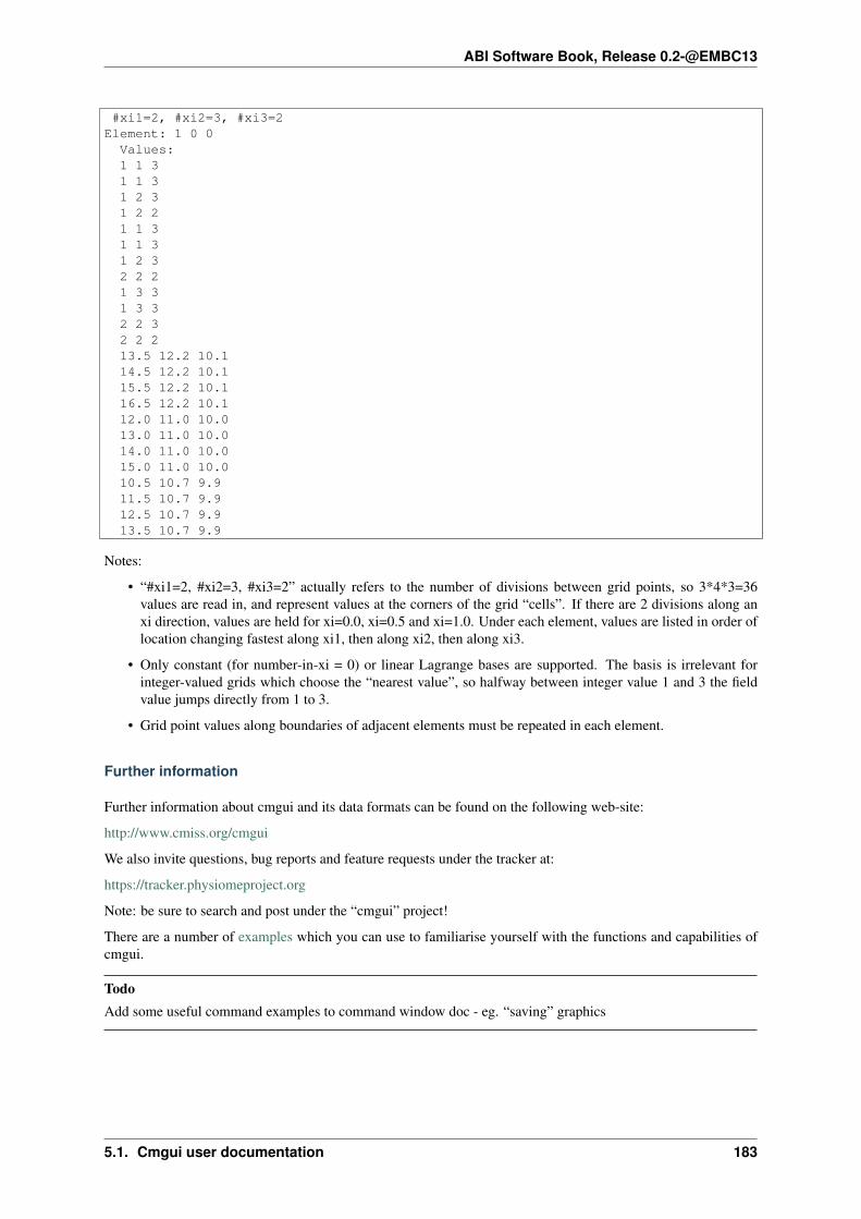
ABI Software Book, Release 0.2-@EMBC13
#xi1=2, #xi2=3, #xi3=2Element: 1 0 0
Values:1 1 31 1 31 2 31 2 21 1 31 1 31 2 32 2 21 3 31 3 32 2 32 2 213.5 12.2 10.114.5 12.2 10.115.5 12.2 10.116.5 12.2 10.112.0 11.0 10.013.0 11.0 10.014.0 11.0 10.015.0 11.0 10.010.5 10.7 9.911.5 10.7 9.912.5 10.7 9.913.5 10.7 9.9
Notes:
• “#xi1=2, #xi2=3, #xi3=2” actually refers to the number of divisions between grid points, so 3*4*3=36values are read in, and represent values at the corners of the grid “cells”. If there are 2 divisions along anxi direction, values are held for xi=0.0, xi=0.5 and xi=1.0. Under each element, values are listed in order oflocation changing fastest along xi1, then along xi2, then along xi3.
• Only constant (for number-in-xi = 0) or linear Lagrange bases are supported. The basis is irrelevant forinteger-valued grids which choose the “nearest value”, so halfway between integer value 1 and 3 the fieldvalue jumps directly from 1 to 3.
• Grid point values along boundaries of adjacent elements must be repeated in each element.
Further information
Further information about cmgui and its data formats can be found on the following web-site:
http://www.cmiss.org/cmgui
We also invite questions, bug reports and feature requests under the tracker at:
https://tracker.physiomeproject.org
Note: be sure to search and post under the “cmgui” project!
There are a number of examples which you can use to familiarise yourself with the functions and capabilities ofcmgui.
TodoAdd some useful command examples to command window doc - eg. “saving” graphics
5.1. Cmgui user documentation 183

ABI Software Book, Release 0.2-@EMBC13
5.2 OpenCMISS user documentation
5.2.1 OpenCMISS concepts
OpenCMISS has the following top level objects.
• Basis Functions
• Coordinate Systems
• Regions
• Problems
• Computational environments
• Base system(Diagnostics, I/O etc.)
Fig. 5.25: OpenCMISS top-level structure
5.2.2 Coordinate Systems
Coordinate system is a system for assigning an n-tuple of numbers or scalars to each point in an n-dimensionalspace. It anchors the regions within the real world. Coordinate system can have different types such as:
• Rectangular cartesian
• Cylindrical polar
• Spherical polar
• Prolate spheroidal
• Oblate spheroidal
184 Chapter 5. Related Software Project at the Auckland Bioengineering Institute

ABI Software Book, Release 0.2-@EMBC13
There is a global (world) coordinate system aligned with 3D rectangular cartesian space.
Coordinate system has the following attributes:
• User number
• Finished tag
• Type
• Number of dimensions
• Focus (for prolate-spheriodal system only)
• Origins
• Orientation
5.2.3 Basis Functions
Basis functions are the key item to specify the field approximation/interpolation and the linking of nodes andelements to form a mesh. Currently, it has two types: Lagrange-Hermite tensor product and Simplex. Lagrange-Hermite tensor product can be further divided into linear to cubic lagrange, cubic and quadratic hermite. It canbe arbitrarily collapsed (two or more nodes in the same location) in any one direction or in any two directions togive a degenerate basis. Simplex basic functions could contain line, triangular and tetrahedral elements. It couldbe linear, quadratic or cubic. Arbitrary Gaussian quadrature can integrate from 1st to 5th order (3rd order forlines at the moment). Can only have the same order in each direction at the moment. Specifying a basis functionautomatically generates all necessary line and face basis functions as sub-bases of the basis function.
Basis function has the following attributes:
• User number
• Global number
• Family number
• Finished tag
• Type
• Is Hermite
• Number of XI
• Number of XI coordinates
• ...
5.2.4 Regions
Regions are one of the primary objects in openCMISS. Regions are hierarchical in nature in that a region can haveone parent region and a number of daughter sub-regions. Daughter regions are related in space to parent regionsby an origin and an orientation of the regions coordinate system. Daughter regions may only have the same orfewer dimensions as the parent region. There is a global (world) region (number 0) that has the global (world)coordinate system.
region_definition.JPG
Region has the following attributes:
• User number
• Finished tag
• Label
• Number of sub(daughter) regions
5.2. OpenCMISS user documentation 185

ABI Software Book, Release 0.2-@EMBC13
• Coordinate system pointer
• Nodes
• Meshes
• Fields
• Equations
• Parent region pointer
• Daughter regions pointers
region_structure.JPG
Nodes
There are three places storing nodal information. Nodes associated with region defines the nodes identificationand the nodes geometric (initial) position.
Node has the following attributes:
• User number
• Global number
• Label
• Initial Position
Meshes
Meshes are topological constructs within a region which fields use to define themselves. Meshes are made up of anumber of mesh components. All mesh components in a mesh must “conform”, that is have the same number ofelements, Xi directions etc.
Mesh has the following attributes:
• User number
• Global number
• Finished tag
• Region pointer
• Number of dimensions
• Number of components
• Embedded flag
• Embedding mesh pointer
• Embedded meshes pointers
• Number of elements
• Number of faces
• Number of lines
• Mesh topology pointers
• Decomposition pointers
mesh_structure.JPG
186 Chapter 5. Related Software Project at the Auckland Bioengineering Institute

ABI Software Book, Release 0.2-@EMBC13
Mesh Topology
Mesh components (Topology) are made up from nodes, elements and basis functions. A new mesh componentis required for each different form of interpolation e.g., one mesh component is bilinear Lagrange and another isbiquadratic Lagrange. meshTopology_definition.JPG
Mesh topology has the following attributes:
• Mesh component number
• Mesh pointer
• Nodes pointers
• Element pointers
• DOFs pointers
meshTopology_structure.JPG
Decompositions
Mesh decomposition (partitioning) is used to split a computationally expensive mesh into smaller subdomains(parts) for parallel computing.
Decomposition has the following attributes:
• User number
• Global number
• Finished tag
• Mesh pointer
• Mesh component number
• Decomposition type
• Number of domains
• Number of edge cut
• Element domain numbers
• Decomposition topology pointer
• Domains pointers(list of domain which has the same size as the number of components in the mesh)
meshDecomposition_structure.JPG
Domain
Each domain stores domain information for relevant mesh component.
The domain object contains the following attributes:
• Decomposition pointer
• Mesh pointer
• Mesh component number
• Region pointer
• Number of dimensions
• Node domain(The domain number that the np’th global node is in for the domain decomposition. Note: thedomain numbers start at 0 and go up to the NUMBER_OF_DOMAINS-1)
• Domain mappings(for each mapped object e.g. nodes, elements, etc)
5.2. OpenCMISS user documentation 187

ABI Software Book, Release 0.2-@EMBC13
• Domain topology pointer(elements, nodes, DOFs)
meshDecompositionDomain_structure.JPG
Domain Mappings
Stores information for each mapped object e.g. nodes, elements, etc.
The domain mapping contains the following attributes:
• Number of local
• Total number of local
• Numbers of domain local
• Number of global
• Number of domains
• Number of internal
• Internal list
• Number of boundary
• Boundary list
• Number of ghost
• Ghost list
• Local to global map
• Global to local map
• Number of adjacent domains
• Pointer to list of adjacent domains by domain number
• List of adjacent domains
meshDecompositionDomainMapping_structure.JPG
Fields
Fields are the central object for storing information and framing the problem. Fields have a number of fieldvariables i.e., u, du/dn, du/dt, d2u/dt2. Each field variable has a number of components. A field is defined on adecomposed mesh. Each field variable component is defined on a decomposed mesh component.
Field can contains the following attributes:
• User number
• Global number
• Finished tag
• Region pointer
• Type(Geometric, Fibre, General, Material, Source)
• Dependent type(Independent, Dependent)
• Dimension
• Decomposition pointer
• Number of variables
• Variables
188 Chapter 5. Related Software Project at the Auckland Bioengineering Institute

ABI Software Book, Release 0.2-@EMBC13
• Scalings sets
• Mappings(DOF->Field parameters)
• Parameter sets(distributed vectors)
• Geometric field pointer
• Geomatric field parameters
• Create values cache
field_structure.JPG
Field variable
Field variable stores variables for the field such as dependent variables. For example, in the Laplace’s equa-tion(FEM), it stores two variables: u and du/dn. Each field variable has a number of components.
Field variable has the following attributes:
• Variable number
• Variable type
• Field pointer
• Region pointer
• Max number of interpolation parameters
• Number of DOFs
• Total number of DOFs
• Global DOF List
• Domain mapping pointer
• Number of components
• Components
Field Variable Component
Field Variable Component has the following attributes:
• Component number
• Variable pointer
• Field pointer
• Interpolation type
• Mesh component number
• Scaling index
• Domain pointer
• Max number of interpolation parameters
• Mappings(Field paramters->DOF)
5.2. OpenCMISS user documentation 189

ABI Software Book, Release 0.2-@EMBC13
Parameter set
Parameter set stores values for each field variable component.
field_parameter_set_definition.JPG
Parameter set has the following Attributes:
• Set index
• Set type
• Parameters pointer
Equation Sets
Equations sets are aimed to have multiple classes, e.g. Elasticity, Fluid mechanics, Electromagnetics, Generalfield problems, Fitting, Optimisation. Different equations are within each class, e.g. Bidomain, Navier-stokes etc.Each equation can use different solution techniques, e.g. FEM, BEM, FD, GFEM. The equation set is associatedwith a region and is built using the fields defined on the region.
The numerical methods are used which will result in a discretised matrix-vector form of the governing equations.openCMISS is designed to generate equations sets with a number of “equations” matrices.
e.g, damped mass spring system Mu + Cu + Ku = f will be represented as:
fieldEquationsets-matrix.JPG
Equations Set has the following attributes:
• User number
• Global number
• Finished tag
• Region pointer
• Class identifier
• Type identifier
• Sub type identifier
• Linearity type(?)
• Time dependence type(?)
• Solution method
• Geometry (fibre?) field pointer
• Materials field pointer
• Source field pointer
• Dependent field pointer
• Analytic info pointer(Analytic info stored in dependent field currently)
• Fixed conditions
• Equations pointer
fieldEquationssets-structure.JPG
190 Chapter 5. Related Software Project at the Auckland Bioengineering Institute

ABI Software Book, Release 0.2-@EMBC13
Equations
Equation holds the matrices and mapping information.
The Field variable to matrix mappings maps each field variable onto the equations matrices or RHS vector.
e.g. Laplace(FEM): 2 variables, 1 component fieldEquationsetsEquations-mappingFEM.JPG
e.g. Laplace(BEM): 2 variables, 1 component fieldEquationsetsEquations-mappingBEM.JPG
e.g. Heat equation(explicit time/FEM space): 2 variables, 1 component fieldEquationsetsEquations-mappingHeat.JPG
TODO matrix distribution
Equations has the following attributes:
• Equation set pointer
• Finished tag
• Output type
• Sparsity type
• Interpolation pointer
• Linear equation data pointer
• Nonlinear equation data pointer
• Time(non-static) data pointer
• Equations mapping pointer
• Equations Matrices
5.2.5 Problems
A problem has a number of solutions (each with their solver) inside a problem control loop. Problem is associatedwith region via solution which maps to equations sets and hence links to region. Multiple problems can be in thesame region, or multiple regions can work to solve one problem.
Problem has the following attributes:
• User number
• Global number
• Finished tag
• Class
• Type
• Subtype
• Control pointer
• Number of solutions
• Solutions pointer
problem_structure.JPG
5.2. OpenCMISS user documentation 191

ABI Software Book, Release 0.2-@EMBC13
Solutions
Solution has the following attributes:
• Solution number
• Finished tag
• Linear solution data pointer
• Nonlinear solution data pointer
• Time (non-static) solution data pointer
• Equations set to add (the next equations set to add)
• Index of added equations set(the last successfully added equations set)
• Solution mapping(which contains equations sets)
• Solver pointer
Solvers
Solver has the following attributes:
• Solution pointer
• Finished tag
• Solve type
• Output type
• Sparsity type
• Linear solver pointer
• Non-linear solver pointer
• Time integrationn solver pointer
• Eigenproblem solver pointer
• Solver matrices
problemSolutionSolver_structure.JPG
Control
Control has the following attributes:
• Problem pointer
• Finished tag
• Control type
5.2.6 Getting started with OpenCMISS
Tutorial one.
192 Chapter 5. Related Software Project at the Auckland Bioengineering Institute

ABI Software Book, Release 0.2-@EMBC13
5.2.7 Using OpenCMISS from Python
Section author: Adam Reeve
In this tutorial we will walk through how to solve Laplace’s equation on a 2D geometry using the Python bindingsto OpenCMISS.
Getting Started
The Python code given here follows the Python Laplace example found in the OpenCMISS examples repository.You can run the code interactively by entering it directly into the Python interpreter, which can be started byrunning python. Alternatively you can enter the code into a text file with a .py extension and run it using thepython command, eg:
python LaplaceExample.py
In order to use OpenCMISS we have to first import the CMISS module from the opencmiss package:
from opencmiss import CMISS
Assuming OpenCMISS has been correctly built with the Python bindings by following the instructions in theprogrammer documentation, we can now access all the OpenCMISS functions, classes and constants under theCMISS namespace.
Create a Coordinate System
First we construct a coordinate system that will be used to describe the geometry in our problem. The 2D geometrywill exist in a 3D space, so we need a 3D coordinate system.
When creating an object in OpenCMISS there are at least three steps. First we initialise the object:
coordinateSystem = CMISS.CoordinateSystem()
This creates a thin wrapper that just points to the actual coordinate system used internally by OpenCMISS, andinitially the pointer is null. Trying to use the coordinate system now would raise an exception. To actuallyconstruct a coordinate system we call the CreateStart method and pass it a user number. The user numbermust be unique between objects of the same type and can be used to identify the coordinate system later. MostOpenCMISS classes require a user number when creating them, and many also require additional parameters tothe CreateStart method:
coordinateSystemUserNumber = 1coordinateSystem.CreateStart(coordinateSystemUserNumber)
We can now optionally set any properties on the object. We will set the dimension so that the coordinate systemis 3D:
coordinateSystem.dimension = 3
And finally, we finish creating the coordinate system:
coordinateSystem.CreateFinish()
Create a Region
Next we create a region that our fields will be defined on and tell it to use the 3D coordinate system we createdpreviously. The CreateStart method for a region requires another region as a parameter. We use the worldregion that is created by default so that our region is a subregion of the world region. We can also give the regiona label:
5.2. OpenCMISS user documentation 193

ABI Software Book, Release 0.2-@EMBC13
regionUserNumber = 1region = CMISS.Region()region.CreateStart(regionUserNumber, CMISS.WorldRegion)region.label = "LaplaceRegion"region.coordinateSystem = coordinateSystemregion.CreateFinish()
Create a Basis
The finite element description of our fields requires a basis function to interpolate field values over elements, sowe create a 2D basis with linear Lagrange interpolation in both xi directions:
basisUserNumber = 1basis = CMISS.Basis()basis.CreateStart(basisUserNumber)basis.type = CMISS.BasisTypes.LAGRANGE_HERMITE_TPbasis.numberOfXi = 2basis.interpolationXi = [
CMISS.BasisInterpolationSpecifications.LINEAR_LAGRANGE,CMISS.BasisInterpolationSpecifications.LINEAR_LAGRANGE,
]basis.quadratureNumberOfGaussXi = [2, 2]basis.CreateFinish()
When we set the basis type we select a value from the BasisTypes enum. To get a list of possible basis typesand interpolation types you can use the help function in the python interpreter:
help(CMISS.BasisTypes)help(CMISS.BasisInterpolationSpecifications)
Similarly, you can see what methods and properties are available for the various CMISS classes and get helpinformation for these:
help(CMISS.Basis)help(CMISS.Basis.CreateStart)help(CMISS.Basis.interpolationXi)
Create a Decomposed Mesh
In order to define a simple 2D geometry for our problem we can use one of OpenCMISS’s inbuilt generatedmeshes. We will create a 2D, rectangular mesh with 10 elements in both the x and y directions and tell it to usethe basis we created previously:
generatedMeshUserNumber = 1numberGlobalXElements = 10numberGlobalYElements = 10width = 1.0length = 1.0
generatedMesh = CMISS.GeneratedMesh()generatedMesh.CreateStart(generatedMeshUserNumber, region)generatedMesh.type = CMISS.GeneratedMeshTypes.REGULARgeneratedMesh.basis = [basis]generatedMesh.extent = [width, length, 0.0]generatedMesh.numberOfElements = [
numberGlobalXElements,numberGlobalYElements]
When setting the basis property, we assign a list of bases as we might want to construct a mesh with multiplecomponents using different interpolation schemes.
194 Chapter 5. Related Software Project at the Auckland Bioengineering Institute

ABI Software Book, Release 0.2-@EMBC13
The generated mesh is not itself a mesh, but is used to create a mesh. We construct the mesh when we call theCreateFinish method of the generated mesh and pass in the mesh to generate:
meshUserNumber = 1mesh = CMISS.Mesh()generatedMesh.CreateFinish(meshUserNumber, mesh)
Here we have initialised a mesh but not called CreateStart or CreateFinish, instead the mesh creation isdone when finishing the creation of the generated mesh.
Because OpenCMISS can solve problems on multiple computational nodes, it must work with a decomposedmesh. We now decompose our mesh by getting the number of computational nodes and creating a decompositionwith that number of domains:
decompositionUserNumber = 1decomposition = CMISS.Decomposition()decomposition.CreateStart(decompositionUserNumber, mesh)decomposition.type = CMISS.DecompositionTypes.CALCULATEDdecomposition.numberOfDomains = CMISS.ComputationalNumberOfNodesGet()decomposition.CreateFinish()
Note that even when we have just one computational node, OpenCMISS still needs to work with a decomposedmesh, which will have one domain.
Defining Geometry
Now that we have a decomposed mesh, we can begin defining the fields we need on it. First we will create ageometric field to define our problem geometry:
geometricFieldUserNumber = 1geometricField = CMISS.Field()geometricField.CreateStart(geometricFieldUserNumber, region)geometricField.meshDecomposition = decompositiongeometricField.ComponentMeshComponentSet(CMISS.FieldVariableTypes.U, 1, 1)geometricField.ComponentMeshComponentSet(CMISS.FieldVariableTypes.U, 2, 1)geometricField.ComponentMeshComponentSet(CMISS.FieldVariableTypes.U, 3, 1)geometricField.CreateFinish()
The call to the ComponentMeshComponentSet method is not actually required here as all field componentswill default to use the first mesh component, but if we have defined a mesh that has multiple components (thatuse different interpolation schemes) then different field components can use different mesh components. Forexample, in a finite elasticity problem we could define our geometry using quadratic Lagrange interpolation, andthe hydrostatic pressure using linear Lagrange interpolation.
We have created a field but all the field component values are currently set to zero. We can define the geometryusing the generated mesh we created earlier:
generatedMesh.GeometricParametersCalculate(geometricField)
Setting up Equations
Now we have a geometric field we can construct an equations set. This defines the set of equations that we wishto solve in our problem on this region. The specific equation set we are solving is defined by the fourth, fifth andsixth parameters to the CreateStart method. These are the equations set class, type and subtype respectively.In this example we are solving the standard Laplace equation which is a member of the classical field equationsset class and the Laplace equation type. When we create an equations set we also have to create an equations setfield, however, this is only used to identify multiple equations sets of the same type on a region so we will not useit:
5.2. OpenCMISS user documentation 195

ABI Software Book, Release 0.2-@EMBC13
equationsSetUserNumber = 1equationsSetFieldUserNumber = 2equationsSetField = CMISS.Field()equationsSet = CMISS.EquationsSet()equationsSet.CreateStart(equationsSetUserNumber, region, geometricField,
CMISS.EquationsSetClasses.CLASSICAL_FIELD,CMISS.EquationsSetTypes.LAPLACE_EQUATION,CMISS.EquationsSetSubtypes.STANDARD_LAPLACE,equationsSetFieldUserNumber, equationsSetField)
equationsSet.CreateFinish()
Now we use our equations set to create a dependent field. This stores the solution to our equations:
dependentFieldUserNumber = 3dependentField = CMISS.Field()equationsSet.DependentCreateStart(dependentFieldUserNumber, dependentField)equationsSet.DependentCreateFinish()
We haven’t used the Field.CreateStart method to construct the dependent field but have had it automati-cally constructed by the equations set.
We can initialise our solution with a value we think will be close to the final solution. A field in OpenCMISS cancontain multiple field variables, and each field variable can have multiple components. For the standard Laplaceequation, the dependent field only has a U variable which has one component. Field variables can also havedifferent field parameter sets, for example we can store values at a previous time step in dynamic problems. Inthis example we are only interested in the VALUES parameter set:
componentNumber = 1initialValue = 0.5dependentField.ComponentValuesInitialiseDP(
CMISS.FieldVariableTypes.U,CMISS.FieldParameterSetTypes.VALUES,componentNumber, initialValue)
Once the equations set is defined, we create the equations that use our fields to construct equations matricesand vectors. We will use sparse matrices to store the equations and enable matrix output when assembling theequations:
equations = CMISS.Equations()equationsSet.EquationsCreateStart(equations)equations.sparsityType = CMISS.EquationsSparsityTypes.SPARSEequations.outputType = CMISS.EquationsOutputTypes.MATRIXequationsSet.EquationsCreateFinish()
Defining the Problem
Now that we have defined all the equations we will need we can create our problem to solve. We create a standardLaplace problem, which is a member of the classical field problem class and Laplace equation problem type:
problemUserNumber = 1problem = CMISS.Problem()problem.CreateStart(problemUserNumber)problem.SpecificationSet(CMISS.ProblemClasses.CLASSICAL_FIELD,
CMISS.ProblemTypes.LAPLACE_EQUATION,CMISS.ProblemSubTypes.STANDARD_LAPLACE)
problem.CreateFinish()
The problem type defines a control loop structure that is used when solving the problem. We may have multiplecontrol loops with nested sub loops, and control loops can have different types, for example load incremented loopsor time loops for dynamic problems. In this example a simple, single iteration loop is created without any subloops. If we wanted to access the control loop and modify it we would use the problem.ControlLoopGetmethod before finishing the creation of the control loops, but we will just leave it with the default configuration:
196 Chapter 5. Related Software Project at the Auckland Bioengineering Institute

ABI Software Book, Release 0.2-@EMBC13
problem.ControlLoopCreateStart()problem.ControlLoopCreateFinish()
Configuring Solvers
After defining the problem structure we can create the solvers that will be run to actually solve our problem. Theproblem type defines the solvers to be set up so we call problem.SolversCreatStart to create the solversand then we can access the solvers to modify their properties:
solver = CMISS.Solver()problem.SolversCreateStart()problem.SolverGet([CMISS.ControlLoopIdentifiers.NODE], 1, solver)solver.outputType = CMISS.SolverOutputTypes.SOLVERsolver.linearType = CMISS.LinearSolverTypes.ITERATIVEsolver.linearIterativeAbsoluteTolerance = 1.0e-10solver.linearIterativeRelativeTolerance = 1.0e-10problem.SolversCreateFinish()
Note that we initialised a solver but didn’t create it directly by calling its CreateStart method, it was createdwith the call to SolversCreateStart and then we obtain it with the call to SolverGet. If we look at thehelp for the SolverGet method we see it takes three parameters:
controlLoopIdentifiers A list of integers used to identify the control loop to get a solver for. This always startswith the root control loop, given by CMISS.ControlLoopIdentifiers.NODE. In this example weonly have the one control loop and no sub loops.
solverIndex The index of the solver to get, as a control loop may have multiple solvers. In this case there is onlyone solver in our root control loop.
solver An initialised solver object that hasn’t been created yet, and on return it will be the solver that we askedfor.
Once we’ve obtained the solver we then set various properties before finishing the creation of all the problemsolvers.
After defining our solver we can create the equations for the solver to solve by adding our equations sets to thesolver equations. In this example we have just one equations set to add but for coupled problems we may havemultiple equations sets in the solver equations. We also tell OpenCMISS to use sparse matrices to store our solverequations:
solverEquations = CMISS.SolverEquations()problem.SolverEquationsCreateStart()solver.SolverEquationsGet(solverEquations)solverEquations.sparsityType = CMISS.SolverEquationsSparsityTypes.SPARSEequationsSetIndex = solverEquations.EquationsSetAdd(equationsSet)problem.SolverEquationsCreateFinish()
Setting Boundary Conditions
The final step in configuring the problem is to define the boundary conditions to be satisfied. We will set thedependent field value at the first node to be zero, and at the last node to be 1.0. These nodes will correspond toopposite corners in our geometry. Because OpenCMISS can solve our problem on multiple computational nodeswhere each computational node does not necessarily know about all nodes in our mesh, we must first check thatthe node we are setting the boundary condition at is in our computational node domain:
nodes = CMISS.Nodes()region.NodesGet(nodes)firstNodeNumber = 1lastNodeNumber = nodes.numberOfNodesfirstNodeDomain = decomposition.NodeDomainGet(firstNodeNumber, 1)lastNodeDomain = decomposition.NodeDomainGet(lastNodeNumber, 1)
5.2. OpenCMISS user documentation 197

ABI Software Book, Release 0.2-@EMBC13
computationalNodeNumber = CMISS.ComputationalNodeNumberGet()
boundaryConditions = CMISS.BoundaryConditions()solverEquations.BoundaryConditionsCreateStart(boundaryConditions)if firstNodeDomain == computationalNodeNumber:
boundaryConditions.SetNode(dependentField, CMISS.FieldVariableTypes.U,1, 1, firstNodeNumber, 1,CMISS.BoundaryConditionsTypes.FIXED, 0.0)
if lastNodeDomain == computationalNodeNumber:boundaryConditions.SetNode(
dependentField, CMISS.FieldVariableTypes.U,1, 1, lastNodeNumber, 1,CMISS.BoundaryConditionsTypes.FIXED, 1.0)
solverEquations.BoundaryConditionsCreateFinish()
When setting a boundary condition at a node we can use either the AddNode method or the SetNode method.Using AddNode will add the value we provide to the current field value and set this as the boundary conditionvalue, but here we want to directly specify the value so we use the SetNode method.
The arguments to the SetNode method are the field, field variable type, node version number, node user number,node derivative number, field component number, boundary condition type and boundary condition value. Theversion and derivative numbers are one as we aren’t using versions and we are setting field values rather thanderivative values. We can also only set derivative boundary conditions when using a Hermite basis type. Thereare a wide number of boundary condition types that can be set but many are only available for certain equation settypes and in this example we simply want to fix the field value.
When solverEquations.BoundaryConditionsCreateFinish() is called OpenCMISS will con-struct the solver matrices and vectors.
Solving
After our problem solver equations have been fully defined we are now ready to solve our problem. When wecall the Solve method of the problem it will loop over the control loops and control loop solvers to solve ourproblem:
problem.Solve()
Exporting the Solution
Once the problem has been solved, the dependent field contains the solution to our problem. We can then exportthe dependent and geometric fields to a FieldML file so that we can visualise the solution using cmgui. We willexport the geometric and dependent field values to a LaplaceExample.xml file. Separate plain text data fileswill also be created:
baseName = "laplace"dataFormat = "PLAIN_TEXT"fml = CMISS.FieldMLIO()fml.OutputCreate(mesh, "", baseName, dataFormat)fml.OutputAddFieldNoType(
baseName + ".geometric", dataFormat, geometricField,CMISS.FieldVariableTypes.U, CMISS.FieldParameterSetTypes.VALUES)
fml.OutputAddFieldNoType(baseName + ".phi", dataFormat, dependentField,CMISS.FieldVariableTypes.U, CMISS.FieldParameterSetTypes.VALUES)
fml.OutputWrite("LaplaceExample.xml")fml.Finalise()
198 Chapter 5. Related Software Project at the Auckland Bioengineering Institute

ABI Software Book, Release 0.2-@EMBC13
5.2.8 Using CellML in OpenCMISS
The aim of this tutorial is to give the user a bit of help in using CellML models in OpenCMISS.OpenCMISS(cellml) is the code that provides the mapping from OpenCMISS(cm) (Fortran) to the CellML API(C++). The API exposed by the OpenCMISS(cellml) library is then wrapped by the OpenCMISS(cm) API,with documentation available in the OpenCMISS programmer documentation. The programmer documenta-tion provides the reference documentation for the OpenCMISS(cm) routines which are described in this tu-torial. The monodomain example from the OpenCMISS examples repository provides a good demonstrationof OpenCMISS+CellML in practice, while the CellML examples are used to perform functional testing of theOpenCMISS(cellml) library.
Overview
OpenCMISS encapsulates all interaction with CellML models within a CellML environment. A CellML environ-ment is specific to a region, but each region may contain zero or more CellML environments. Having created aCellML environment you are then able to import CellML models into the environment. Each CellML environmentmay import an arbitrary number of CellML models. [TODO: what is a use-case for multiple CellML environmentsin a region?]
Variables in CellML models imported into a CellML environment are then able to flagged as known or wanted asdesired by the user. Flagged variables are made available by the CellML environment for mapping to OpenCMISSfields, either for obtaining values from the CellML model (wanted) or setting values in the CellML model (known).
In order for the CellML environment to mange the computation of a CellML model, each environment requiresthe user to provide several fields suitable for such usage. These are the models, state, intermediate, and param-eters fields. Typically the user will pass in empty fields and allow the CellML environment to create the fieldsappropriately.
With all desired fields set-up appropriately, the user then just needs to add their CellML environment(s) to thecorresponding solver as part of their control loop set-up when defining the actual problem to solve.
The CellML environment
The OpenCMISS type for the CellML environment is CMISSCellMLType. As with most OpenCMISS types,a user-number is provided to uniquely identify this CellML environment to the user. The basic creation block isgiven below.
! declare the user number for the CellML environment we want to createINTEGER(CMISSIntg), PARAMETER :: CellMLUserNumber=10! and the actual handle for the CellML environmentTYPE(CMISSCellMLType) :: CellML
! We first initialise the CellML environmentCALL CMISSCellML_Initialise(CellML,Err)! and then we are able to trigger the start of creationCALL CMISSCellML_CreateStart(CellMLUserNumber,Region,CellML,Err)
! import models
! flag variables
! terminate the creation processCALL CMISSCellML_CreateFinish(CellML,Err)
It is important to note that all required models must be imported and all desired variables flagged before terminat-ing the CellML environment creation process. This is because the create finish method will proceed to make use ofOpenCMISS(cellml) to instantiate each of the imported CellML models into executable code, and the generationof that executable code requires all knowledge of the flagged variables.
Models are imported into the CellML environment with the code shown below.
5.2. OpenCMISS user documentation 199

ABI Software Book, Release 0.2-@EMBC13
INTEGER(CMISSIntg) :: modelIndex
! Import the specified model into the CellML environmentCALL CMISSCellML_ModelImport(CellML,"model.xml",modelIndex,Err)
In this example, the CellML model model.xml is imported into the CellML environment andon successful return the variable modelIndex will be set to the index for this specific modelin the CellML environment. The CellML model to import is specified by URL, and canbe either absolute (e.g., http://example.com/coolest/model/ever.xml) or relative (e.g.,coolest/model/ever.xml). If a relative URL is specified, it will be resolved relative to the current workingdirectory (CWD) of the executed application. (It is anticipated that application developers would use their ownlogic to provide absolute URLs to define CellML models in OpenCMISS.)
Flagging variables
As mentioned above, all variables of interest in the imported CellML models must be flagged prior to terminatingthe CellML environment creation process. Variables in CellML models can be flagged as either known or wanted.Flagging variables in a model will inform OpenCMISS(cellml) that the given variable(s) need to be available foruse by OpenCMISS(cm), and hence the executable code generated when the models are instantiated is required toprovide this access. The process for flagging variables is shown below.
! Flag a variable as knownCALL CMISSCellML_VariableSetAsKnown(CellML,modelIndex,"fast_sodium_current/g_Na ",Err)! Flag a variable as wantedCALL CMISSCellML_VariableSetAsWanted(CellML,modelIndex,"membrane/i_K1",Err)
Details on how to identify specific variables in a CelLML model are given below. The modelIndex should bethe index of the desired model in the CellML environment, as returned by the model import described above.
Flagging a variable as known indicates that the OpenCMISS user wants to control the value of the specifiedvariable, thus taking ownership of the variable from the CellML model. Currently, only CONSTANT variables inCellML models can be flagged as known (see the Variable Evaluation Types in the CellML API documentation).This is typically used when parameters in the CellML model are to have their values defined by OpenCMISSfields.
Flagging a variable as wanted indicates that the OpenCMISS user wants to obtain the value of the specified variablefrom the CellML model. Currently, CONSTANT, PSEUDOSTATE_VARIABLE, and ALGEBRAIC variables inCellML models can be flagged as wanted (see the Variable Evaluation Types in the CellML API documentation).In order to be able to save the state of CellML models during integration steps, all state variables in modelsare automatically flagged as wanted. Depending on how the CellML model is being applied in the OpenCMISSsimulation, variables that are considered CONSTANT by the CelLML API will actually be the variables of interestto the OpenCMISS user - commonly the case for mechanical constitutive relationships where the wanted strainenergy components are algebraically related to the known strain components.
Identifying CellML variables
When identifying variables from CellML models in OpenCMISS, the convention is to address them with a stringconsisting of the variable’s name and the name of the parent component. Given the following (invalid!) CellMLmodel,
<model><import href="http://models.cellml.org/bob/model.xml"><component name="imported_component" component_ref="source_component"/>
</import><component name="membrane"><variable name="i_K1"/><variable name="i_stimulus"/><variable name="T"/>
</component>
200 Chapter 5. Related Software Project at the Auckland Bioengineering Institute
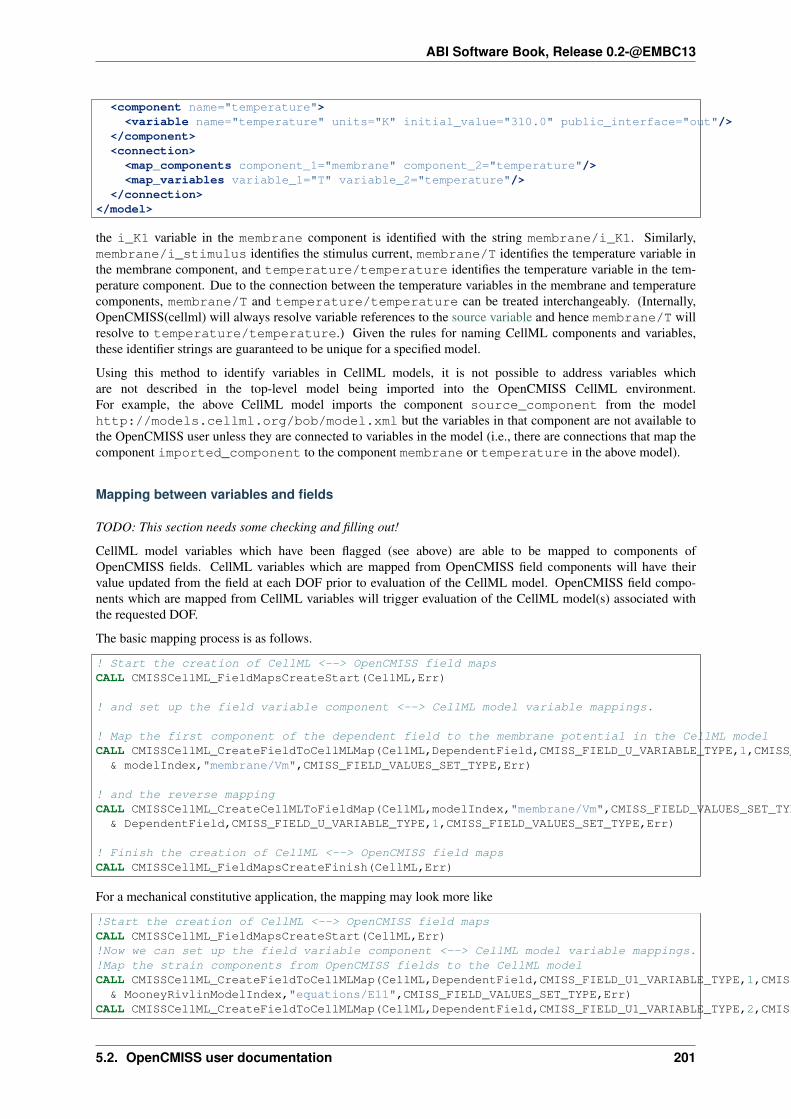
ABI Software Book, Release 0.2-@EMBC13
<component name="temperature"><variable name="temperature" units="K" initial_value="310.0" public_interface="out"/>
</component><connection><map_components component_1="membrane" component_2="temperature"/><map_variables variable_1="T" variable_2="temperature"/>
</connection></model>
the i_K1 variable in the membrane component is identified with the string membrane/i_K1. Similarly,membrane/i_stimulus identifies the stimulus current, membrane/T identifies the temperature variable inthe membrane component, and temperature/temperature identifies the temperature variable in the tem-perature component. Due to the connection between the temperature variables in the membrane and temperaturecomponents, membrane/T and temperature/temperature can be treated interchangeably. (Internally,OpenCMISS(cellml) will always resolve variable references to the source variable and hence membrane/T willresolve to temperature/temperature.) Given the rules for naming CellML components and variables,these identifier strings are guaranteed to be unique for a specified model.
Using this method to identify variables in CellML models, it is not possible to address variables whichare not described in the top-level model being imported into the OpenCMISS CellML environment.For example, the above CellML model imports the component source_component from the modelhttp://models.cellml.org/bob/model.xml but the variables in that component are not available tothe OpenCMISS user unless they are connected to variables in the model (i.e., there are connections that map thecomponent imported_component to the component membrane or temperature in the above model).
Mapping between variables and fields
TODO: This section needs some checking and filling out!
CellML model variables which have been flagged (see above) are able to be mapped to components ofOpenCMISS fields. CellML variables which are mapped from OpenCMISS field components will have theirvalue updated from the field at each DOF prior to evaluation of the CellML model. OpenCMISS field compo-nents which are mapped from CellML variables will trigger evaluation of the CellML model(s) associated withthe requested DOF.
The basic mapping process is as follows.
! Start the creation of CellML <--> OpenCMISS field mapsCALL CMISSCellML_FieldMapsCreateStart(CellML,Err)
! and set up the field variable component <--> CellML model variable mappings.
! Map the first component of the dependent field to the membrane potential in the CellML modelCALL CMISSCellML_CreateFieldToCellMLMap(CellML,DependentField,CMISS_FIELD_U_VARIABLE_TYPE,1,CMISS_FIELD_VALUES_SET_TYPE, &
& modelIndex,"membrane/Vm",CMISS_FIELD_VALUES_SET_TYPE,Err)
! and the reverse mappingCALL CMISSCellML_CreateCellMLToFieldMap(CellML,modelIndex,"membrane/Vm",CMISS_FIELD_VALUES_SET_TYPE, &
& DependentField,CMISS_FIELD_U_VARIABLE_TYPE,1,CMISS_FIELD_VALUES_SET_TYPE,Err)
! Finish the creation of CellML <--> OpenCMISS field mapsCALL CMISSCellML_FieldMapsCreateFinish(CellML,Err)
For a mechanical constitutive application, the mapping may look more like
!Start the creation of CellML <--> OpenCMISS field mapsCALL CMISSCellML_FieldMapsCreateStart(CellML,Err)!Now we can set up the field variable component <--> CellML model variable mappings.!Map the strain components from OpenCMISS fields to the CellML modelCALL CMISSCellML_CreateFieldToCellMLMap(CellML,DependentField,CMISS_FIELD_U1_VARIABLE_TYPE,1,CMISS_FIELD_VALUES_SET_TYPE, &
& MooneyRivlinModelIndex,"equations/E11",CMISS_FIELD_VALUES_SET_TYPE,Err)CALL CMISSCellML_CreateFieldToCellMLMap(CellML,DependentField,CMISS_FIELD_U1_VARIABLE_TYPE,2,CMISS_FIELD_VALUES_SET_TYPE, &
5.2. OpenCMISS user documentation 201

ABI Software Book, Release 0.2-@EMBC13
& MooneyRivlinModelIndex,"equations/E12",CMISS_FIELD_VALUES_SET_TYPE,Err)CALL CMISSCellML_CreateFieldToCellMLMap(CellML,DependentField,CMISS_FIELD_U1_VARIABLE_TYPE,3,CMISS_FIELD_VALUES_SET_TYPE, &
& MooneyRivlinModelIndex,"equations/E13",CMISS_FIELD_VALUES_SET_TYPE,Err)CALL CMISSCellML_CreateFieldToCellMLMap(CellML,DependentField,CMISS_FIELD_U1_VARIABLE_TYPE,4,CMISS_FIELD_VALUES_SET_TYPE, &
& MooneyRivlinModelIndex,"equations/E22",CMISS_FIELD_VALUES_SET_TYPE,Err)CALL CMISSCellML_CreateFieldToCellMLMap(CellML,DependentField,CMISS_FIELD_U1_VARIABLE_TYPE,5,CMISS_FIELD_VALUES_SET_TYPE, &
& MooneyRivlinModelIndex,"equations/E23",CMISS_FIELD_VALUES_SET_TYPE,Err)CALL CMISSCellML_CreateFieldToCellMLMap(CellML,DependentField,CMISS_FIELD_U1_VARIABLE_TYPE,6,CMISS_FIELD_VALUES_SET_TYPE, &
& MooneyRivlinModelIndex,"equations/E33",CMISS_FIELD_VALUES_SET_TYPE,Err)
! Map the material parameters - if any
! Map the stress components from the CellML model to the OpenCMISS dependent fieldCALL CMISSCellML_CreateCellMLToFieldMap(CellML,MooneyRivlinModelIndex,"equations/Tdev11",CMISS_FIELD_VALUES_SET_TYPE, &
& DependentField,CMISS_FIELD_U2_VARIABLE_TYPE,1,CMISS_FIELD_VALUES_SET_TYPE,Err)CALL CMISSCellML_CreateCellMLToFieldMap(CellML,MooneyRivlinModelIndex,"equations/Tdev12",CMISS_FIELD_VALUES_SET_TYPE, &
& DependentField,CMISS_FIELD_U2_VARIABLE_TYPE,2,CMISS_FIELD_VALUES_SET_TYPE,Err)CALL CMISSCellML_CreateCellMLToFieldMap(CellML,MooneyRivlinModelIndex,"equations/Tdev13",CMISS_FIELD_VALUES_SET_TYPE, &
& DependentField,CMISS_FIELD_U2_VARIABLE_TYPE,3,CMISS_FIELD_VALUES_SET_TYPE,Err)CALL CMISSCellML_CreateCellMLToFieldMap(CellML,MooneyRivlinModelIndex,"equations/Tdev22",CMISS_FIELD_VALUES_SET_TYPE, &
& DependentField,CMISS_FIELD_U2_VARIABLE_TYPE,4,CMISS_FIELD_VALUES_SET_TYPE,Err)CALL CMISSCellML_CreateCellMLToFieldMap(CellML,MooneyRivlinModelIndex,"equations/Tdev23",CMISS_FIELD_VALUES_SET_TYPE, &
& DependentField,CMISS_FIELD_U2_VARIABLE_TYPE,5,CMISS_FIELD_VALUES_SET_TYPE,Err)CALL CMISSCellML_CreateCellMLToFieldMap(CellML,MooneyRivlinModelIndex,"equations/Tdev33",CMISS_FIELD_VALUES_SET_TYPE, &
& DependentField,CMISS_FIELD_U2_VARIABLE_TYPE,6,CMISS_FIELD_VALUES_SET_TYPE,Err)!Finish the creation of CellML <--> OpenCMISS field mapsCALL CMISSCellML_FieldMapsCreateFinish(CellML,Err)
CellML fields
The required fields and what you might want to do with them...
Evaluating CellML fields
Do we want to describe how simple algebraic-type evaluation can be done independently of the wholesolver/problem/equation set thingy? is that even possible?
Adding CellML models to your Problem set-up
Really need a better title! Explain how CellML environments get added into control loops, etc. so that they getcomputed along with the rest of the model when performing a simulation.
Miscellaneous utilities
Collect all the other bits and pieces here? these are typically the OpenCMISS(cellml) functions that are usedinternally by OpenCMISS(cm) but maybe should be (and are?) exposed via the OpenCMISS(cm) API?
5.2.9 OpenCMISS tutorial videos
Videos of OpenCMISS tutorials.
MPI tutorial 31 January 2012 Chris Bradley
CUDA tutorial 1 17 February 2012 Chris Bradley
CUDA tutorial 2 24 February 2012 Chris Bradley
OpenMP tutorial 16 March 2012 Chris Bradley
202 Chapter 5. Related Software Project at the Auckland Bioengineering Institute

ABI Software Book, Release 0.2-@EMBC13
Contact Mechanics tutorial 17 August 2012 Nancy Yan
Bidomain tutorial
5.2.10 Tutorial: Version Control With Git
Section author: Adam Reeve
Getting Started
If Git isn’t installed already, it can be installed from the git-core package if you’re using Linux or by downloadingmsysGit for Windows.
The first thing that must be done before using Git is to tell it your name and email address. These will be associatedwith any commits you make:
git config --global user.name "Adam Reeve"git config --global user.email "[email protected]"
If you are using a graphical Git client such as Tortoise Git on Windows or gitg on Linux there will be an option toedit these settings.
Creating a Repository
You can initialise a new Git repository in an existing directory with:
git init
Or to create a new directory:
git init my_project
Cloning an Existing Repository
You can clone an existing repository from a local path or from a URL. To clone the repository for this tutorial,run:
git clone https://github.com/adamreeve/git_tutorial.git
This will create a git_tutorial directory in your current directory, so change into that directory now:
cd git_tutorial
Have a look at the project history on the master branch with:
git log
Also try out some of the options to the log command:
git log --patchgit log --statgit log --oneline --graph --all
The last example uses the “–all” option to show history in all branches.
5.2. OpenCMISS user documentation 203

ABI Software Book, Release 0.2-@EMBC13
Making and Committing Changes
Run git status and you should get a message that there are no changes to be staged and no staged changes tobe committed.
Now make a change to the hello.py file and run git status again. You should see that you still have nochanges staged to commit but you have an unstaged change.
Run git diff go see what changes you have made. Now add your change to the staging area:
git add hello.py
And run git status again. You will see that there are no unstaged changes but one file has changes that arestaged.
Now run git diff and there should be no changes. This is because git diff compares your workingdirectory with the staging area by default. To see what changes are in the staging area and would be committed,run:
git diff --cached
If you’ve decided that you no longer want to commit a change that you’ve added to the staging area, you’ll needto unstage that file by running:
git reset HEAD hello.py
Note: git tells you how to stage and unstage changes in the output of the git status command.
If you then decide that your change is rubbish and you want to remove it completely, you can checkout a cleanversion of the changed file:
git checkout -- hello.py
The “–” before the file path isn’t required but is recommended as it means that any further command options arefile paths, which prevents confusion when you have a file named the same as a branch (as git checkout isalso used for checking out a branch, as you’ll see later).
Now make another change and add it to the staging area, then commit it:
git commit -m "My awesome change"
You can either specify a commit message on the command line with the “-m” option or if you leave that option off,git will open a text editor to allow you to enter a message. By default this is vim, but you might want to change itto something else. For example, if you’re on Linux:
git config --global core.editor "gedit"
Or if you’re on Windows and have TortoiseGit installed, you can use:
git config --global core.editor "notepad2"
Now make another change to the file and then add this change to the staging area, then run:
git commit --amend
The amend option lets you update the previous commit. It will also open the editor to let you update the commitmessage if required. This is useful if you realise you’ve made a small mistake in the previous commit and haven’tyet pushed it to a public repository.
Note: The commit hash changes after you amend it. This is now a different commit to the one before, so the hashhas changed.
Now we’ll try using git’s graphical interface for making a commit. Make a change to hello.py then run:
204 Chapter 5. Related Software Project at the Auckland Bioengineering Institute

ABI Software Book, Release 0.2-@EMBC13
git gui
Stage the change you made then make another commit.
Branches
It’s always a good idea to create a new branch for any new feature you’re working on in a project:
git branch new_feature
This will create a new branch that points to the commit you have currently checked out. You can also specify whichcommit the new branch should point to. For example, to create a new branch that points to the same commit asthe master branch:
git branch another_feature master
To delete a branch:
git branch -d another_feature
This will give an error if the branch hasn’t been merged into another branch.
Now checkout the branch you created. If there are any differences between your previous head commit and thebranch you are checking out, your working directory will be updated:
git checkout new_feature
You can create a new branch and check it out in one go by using the “-b” option to the checkout command:
git checkout -b my_feature
Now make some changes and commit them on your new branch. You can see a list of branches and the branchyou’re on at any time by running:
git branch
Have a look at the history of your branch and the position of other branches by running gitk.
Merging and Resolving Conflicts
Now we will practice merging one branch into another branch. We will create a new local branch that matchesthe “merge_into” branch from the origin repository, and merge in the “merge_from” branch. First create the localbranch you will work on:
git checkout -b merge_into origin/merge_into
Now run:
gitk --all
This will show a tree with commits from all branches. Note where the heads of the merge_from, ori-gin/merge_from and origin/merge_into branches are.
Now merge the origin/merge_from branch:
git merge origin/merge_from
And look at the result of your merge:
gitk --all
Now we will try another merge, but this time there will be a conflict:
5.2. OpenCMISS user documentation 205

ABI Software Book, Release 0.2-@EMBC13
git checkout -b merge_conflict origin/merge_conflictgitk --allgit merge origin/conflicting
Read the output of the merge command to note that there is a conflict in the hello.py file. Also run gitstatus. When you have conflicts in multiple files you can keep track of which conflicts have been resolved withthe status command. Open that file in your editor and resolve the conflict. Then mark the conflict as resolved byadding the file:
git add hello.py
And now you have to manually make a merge commit:
git commit -m "Merge conflicting branch"
Remotes and Remote Branches
As you originally cloned this repository, you have one remote repository set up already called “origin”. To list theremote repositories you’ve added with their urls:
git remote -v
Branches on a remote repository can be checked out or referred to in other commands by prefixing them with theremote name. For example, to show the head commit of the master branch on the origin repository:
git show origin/master
To see all branches including those on remote repositories, you can use:
git branch -a
Staging Parts of Files
Most Git graphical interfaces allow you to stage only some changes in a file. From the Git command line you cando this with the “–patch” or “-p” option to the add command. Change a line at the top of hello.py and thenmake another change at the bottom. Now run:
git add -p hello.py
Say yes to adding the first change but no to the second change, then run git status, git diff, and thengit diff --cached.
Stashing Changes
Git’s stash command is useful for storing changes you have made that you want to save but don’t want to commityet. For example, you can stash changes and then switch to another branch and do some work, making commits,then go to another branch and recover your stashed changes.
Run git status. You should have a change added to the staging area and another unstaged change from thelast section. Otherwise make a change to hello.py. Now stash those changes:
git stash
And look at what this has done:
git statusgit stash listgit stash show -p stash@{0}
206 Chapter 5. Related Software Project at the Auckland Bioengineering Institute

ABI Software Book, Release 0.2-@EMBC13
Your working directory and index should now be clean, but your change is safely stored away in the list of stashes.
Now pop your stashed change off the top of the stash list:
git stash popgit statusgit diffgit stash list
Your changes are now back in your working directory, and have been removed from the stash list.
Stash your change again to get a clean working directory:
git stash
Note that you can use git stash apply to apply a stashed change without removing it from the stash list,and that you can also apply a stashed change on a different branch to the one it was made on.
Rewriting History
Git has powerful tools for allowing you to rearrange history so that you can clean up work to make the historymore clear. The most useful one to know is git rebase --interactive. Rebasing means to move a seriesof commits onto a new base commit. You can also use the rebase command and keep the base the same, but stilledit and rearrange commits.
Checkout a new branch that points to the same commit as origin/rebase_me:
git checkout -b rebasing origin/rebase_me
We will rebase these commits onto the latest master branch. First have a look at what we willrebasing by running gitk --all and looking at the origin/rebase_me branch, or git log -porigin/master..rebasing.
Now start the interactive rebase:
git rebase --interactive origin/master
Reorder the commits so that the “Update docstring” commit is first and the “Fix typo” commit is squashed intothe “More excitement” commit.
Because you have squashed a commit, you will get the opportunity to change the message of the commit that wassquashed into. Think about whether you should update the original commit message to account for the changethat was squashed.
Run gitk to see what you’ve done.
Note that you can still access any rebased commits by their hash, and you can find the commits that you haverecently checked out with the git reflog command. This means that if you have committed something it’svery hard to permanently lose that work.
More on Remotes
Create an account on GitHub if you don’t have one already, then fork this repository. Now make some changesto this repository (if you can, make the tutorial better!) and push them to a branch on your remote repository. Topush you’ll first have to create an alias for your remote repository:
git remote add github https://<your_username>@github.com/<your_username>/git_tutorial.git
Where “<your_username>” has been replaced with your GitHub username. Now to push your changes to yourremote repository:
git push github <name_of_branch>
5.2. OpenCMISS user documentation 207

ABI Software Book, Release 0.2-@EMBC13
Now on the web page for your fork of the git_tutorial repository, click on the pull request button and follow thesteps to create a new pull request.
• genindex
• search
5.2.11 Laplace examples
42 master
For testing
Analytic Laplace
For testing
Laplace ellipsoid
For testing
Laplace Python
For testing
Laplace
For testing
Laplace C
For testing
Number Laplace
For testing
Parallel Laplace
For testing
208 Chapter 5. Related Software Project at the Auckland Bioengineering Institute

CHAPTER 6
Glossary
Clone Clone is a Mercurial term that means to make a complete copy of a Mercurial repository. This is done inorder to have a local copy of a repository to work in.
Embedded workspace, Embedded workspaces A Mercurial concept that allows workspaces to be nestedwithin other workspaces.
Exposure, Exposures A publicly available page that provides access to and information about a specific revisionof a workspace. Exposures are used to publish the contents of workspaces at points in time where themodel(s) contained are considered to be useful.
Exposures are created by the PMR software, and offer views appropriate to the type of model being exposed.CellML files for example are presented with options such as code generation and mathematics display,whereas FieldML models might offer a 3D view of the mesh.
Fork A copy of the workspace which includes all the original version history, but is owned by the user whocreated the fork.
Mercurial Mercurial is a distributed version control system, used by the Physiome Model Repository softwareto maintain a history of changes to files in workspaces. See a tour of the Mercurial basics for some goodintroductory material.
Pull, Pulling The term used with distributed version control systems for the action of pulling changes from oneclone of the repository into another. With PMR, this usually implies pulling from a workspace in the modelrepository into a clone of the workspace on your local machine.
Push, Pushing The term used with distibuted version control systems for the action of pushing changes fromone clone of the repository into another. With PMR, this usually implies pushing from a workspace cloneon your local machine back to the workspace in the model repository, but could be into any other clone ofthe workspace. See a tour of the Mercurial basics for some good introductory material.
Python Python is a programming language that lets you work more quickly and integrate your systems moreeffectively. See http://python.org for all the details.
Synchronize Used to pull the contents or changes from other Mercurial repositories into a workspace via a URI.
Workspace, Workspaces A Mercurial repository hosted on the Physiome Model Repository. This is essentiallya folder or directory in which files are stored, with the added feature of being version controlled by thedistributed version control system called Mercurial.
209

ABI Software Book, Release 0.2-@EMBC13
210 Chapter 6. Glossary

CHAPTER 7
Tutorial to do list
7.1 General
Todo• Add many more references (.. _like-this:) to docs for cross-referencing.
• make sure all references to the staging instance are updated to teching.physiomeproject.org
7.2 Within sections
Todo• Add many more references (.. _like-this:) to docs for cross-referencing.
• make sure all references to the staging instance are updated to teching.physiomeproject.org
(The original entry is located in /home/docs/checkouts/readthedocs.org/user_builds/abi-software-book/checkouts/latest/ABIBook-TODO.rst, line 10.)
TodoAdd some useful command examples to command window doc - eg. “saving” graphics
(The original entry is located in /home/docs/checkouts/readthedocs.org/user_builds/abi-software-book/checkouts/latest/Cmgui/index.rst, line 34.)
TodoNeed to check this section on obtaining models via mercurial.
(The original entry is located in /home/docs/checkouts/readthedocs.org/user_builds/abi-software-book/checkouts/latest/PMR/PMR-downloading-viewing.rst, line 76.)
TodoThis section needs more work.
(The original entry is located in /home/docs/checkouts/readthedocs.org/user_builds/abi-software-book/checkouts/latest/PMR/PMR-embeddedworkspaces.rst, line 9.)
Todo
211

ABI Software Book, Release 0.2-@EMBC13
• Update all PMR documentation to reflect workspace ID changes and user workspace changes, if they goahead.
• Get embedded workspaces doc written.
• Get some best practice docs written.
(The original entry is located in /home/docs/checkouts/readthedocs.org/user_builds/abi-software-book/checkouts/latest/PMR/index.rst, line 29.)
TodoComplete this section
(The original entry is located in /home/docs/checkouts/readthedocs.org/user_builds/abi-software-book/checkouts/latest/tutorials/embc13/scenario1/bestpractice.rst, line 6.)
TodoThis section.
(The original entry is located in /home/docs/checkouts/readthedocs.org/user_builds/abi-software-book/checkouts/latest/tutorials/embc13/scenario2/bestpractice.rst, line 6.)
TodoComplete this section
(The original entry is located in /home/docs/checkouts/readthedocs.org/user_builds/abi-software-book/checkouts/latest/tutorials/embc13/scenario3/bestpractice.rst, line 6.)
212 Chapter 7. Tutorial to do list

CHAPTER 8
Indices and tables
• genindex
• modindex
• search
8.1 ABI research case studies
Examples of research at the ABI - goals, tools and techniques used, outcomes.
To serve as examples of how to use the available tools, as well as promotional material.
If you would like your research to appear in this section, please let me know, or fork this documentation onGitHub!
8.2 About the ABI
History, research groups, opportunities etc etc.
Contents:
8.2.1 ABI Resources
Documentation covering what resources are available for Msc and PhD students to carry out their research.
Computer hardware and software
• Details of computers available to students.
• Operating system options
• List of software packages available for installation
• License issues
• Information about help, IT staff etc.
213

ABI Software Book, Release 0.2-@EMBC13
workshop
Other
8.2.2 ABI Research Groups
8.3 CAP user documentation
8.4 CM user documentation
8.5 CellML API user documentation
8.6 Exporting ip files for CM from cmgui
You can export files in the ip format used by CM using the gfx export command, for example:
gfx export cm field coordinates ipcoor FILENAME.ipcoor ipbase FILENAME.ipbase ipmap FILENAME.ipmap ipnode FILENAME.ipnode ipelem FILENAME.ipelem region "/"
8.7 Testing MathJax LaTeX support
Just a test. Also, a cheeky little test of PEP 3118: New memoryview implementation and buffer protocol docu-mentation.
8.7.1 First test
(𝑎 + 𝑏)2 = 𝑎2 + 2𝑎𝑏 + 𝑏2
(𝑎− 𝑏)2 = 𝑎2 − 2𝑎𝑏 + 𝑏2
Some text
𝑧
(︃1 +
√︂𝜔𝑖+1 + 𝜁 − 𝑥 + 1
Θ + 1𝑦 + 1
)︃= 1
More intervening text
𝑑
𝑑𝑥
(︂∫︁ 𝑥
0
𝑓(𝑢) 𝑑𝑢
)︂= 𝑓(𝑥).
Does this get stripped?
Probably.
8.8 MAP Client
The MAP Client is a cross-platform framework for managing workflows. MAP Client is a plugin-based applicationthat can be used to create workflows from a collection of workflow steps.
The MAP Client is an application written in Python and based on Qt the cross-platform application and UI frame-work. Further details are available in the documents listed below.
214 Chapter 8. Indices and tables

ABI Software Book, Release 0.2-@EMBC13
8.8.1 MAP Installation and Setup Guide
This document describes how to install and setup the MAP software for use on your machine. The MAP softwareis a Python application that uses the PySide Qt library bindings. The instructions in this document cover theinstallation and setup on a Windows based operating system. The instructions for GNU/Linux and OS X aresimilar and should be extrapolated from these instructions. There are some side notes for these other operatingsystems to help, but not full or dedicated instructions. If for any reason you get stuck and cannot complete theinstructions please contact us.
MAP
The MAP framework is written in Python and is designed to work with Python 2 and Python 3. The MAP appli-cation is tested against Python2.6, Python2.7 and Python3.3 and should work with any of these Python libraries.Currently the MAP framework is not packaged as an application, requiring the user to set up the environment priorto launching the mapclient.py executable Python script.
The MAP application consists of the framework and various tools, by itself it can do very little. It is the job ofthe plugins to provide functionality. The MAP application as referred to in this section of the instructions may bedescribed as the barebones application for this reason.
To execute the barebones application we need to first install some dependencies:
1. Python (and make sure to add the Python and Python\Scripts folders to your systemPATH).
2. PySide (PySide and PyQt4 are virtually interchangeable but currently this would require sometextual changes)
3. Python setup tools and then using easy_install.exe to install:
1. Requests Python library (easy_install requests)
2. OAuthlib Python library (not the OAuth Python library) (easy_install oauthlib).
Also, if we wish to interact with the Physiome Model Repository (PMR) we need:
1. Mercurial
We can now install the barebones MAP client application. The barebones application can be launched via thecommand window with the following command in the extracted mapclient/src folder:
mapclient.py
which should result in an application window similar to that shown below.
8.8. MAP Client 215

ABI Software Book, Release 0.2-@EMBC13
Now that the barebones MAP application is installed and running we can move on to some useful plugins.
MAP Plugins
The installation of MAP plugins simply requires obtaining the plugins and then using the MAP plugin manager tolet the MAP client know where to look for plugins. Furthermore, there is a github project which is used to providea common collection of MAP plugins. For the purposes of this tutorial, the autosegmentationstep pluginwill be used. You can download a copy of the plugin, extract it, and then follow the instructions for adding thefolder in which you extracted the plugin to the MAP plugin manager.
Zinc and PyZinc
Zinc is an advanced field manipulation and visualisation library and PyZinc provides Python bindings to the Zinclibrary. Binaries are available for download for Linux, Windows, and OS X. The MAP client is able to make useof Zinc for advanced visualisation and image processing steps. To get PyZinc installed, follow these steps:
1. Install Zinc using either: the Windows installer (ensuring that you enable the option for the installer to addZinc to the system PATH); or unzip the archive and manually copy library file to somewhere on your PATH(which could include the PyZinc installation folder).
2. Unzip the downloaded PyZinc archive.
3. In a command window, change into folder PyZinc extracted into.
4. Execute the following command: python setup.py install (this uses a similar mechanism as theeasy_instal software above..
You can check that you have Zinc and PyZinc correctly installed and functional by running thevolume_fitting.py application provided with the tutorial materials. If Zinc and PyZinc are working youshould get an application window similar to that shown below with the interactive three-dimensional model viewershown. Note you will need to restart the command window after installing PyZinc in order to refresh the systemPATH.
216 Chapter 8. Indices and tables

ABI Software Book, Release 0.2-@EMBC13
Which Binary?
There are a number of binaries available for any given platform and you must match the package description withyour system setup. The package description contains the package name, package version, package architecture,package operating system and in the case of PyZinc the package Python version. The package extension indicatesthe type of package and they come in two main flavours: installer/package manager; archive.
Additionally the version of the PyZinc binaries you download must match the version of the Zinc library binaries.
8.8.2 MAP Features Demonstration
Section author: Hugh Sorby
Note: MAP is currently under active development, and this document will be updated to reflect any changes tothe software or new features that are added. You can follow the development of MAP at the launchpad project.
This document details the features of MAP, a cross-platform framework for managing workflows. MAP is aplugin-based application that can be used to create workflows from a collection of workflow steps.
In this demonstration is based on version 0.9.0 of MAP, available from the project downloads. Directions forinstalling MAP and getting the MAP plugins are available in the MAP Installation and Setup Guide.
In this demonstration we will cover the features of MAP. We will start with a quick tour and then create a newworkflow that will help us segment a region of interest from a stack of images.
Quick Tour
When you first load MAP, it will look something like this:
In the main window we can see three distinct areas that make up the workflow management side of the software.These three areas are the menu bar (at the top), the step box (on the left) that contains the steps that you can use tocreate your workflow and the workflow canvas (on the right) an area for constructing a workflow.
In the Step box we will only see two steps, this is because we have only loaded the default Steps and not loadedany of the external plugins that MAP can use.
8.8. MAP Client 217

ABI Software Book, Release 0.2-@EMBC13
Menu Bar
The Menu bar provides a selection of drop down menus for accessing the applications functions. The File menuprovides access to opening, importing, closing workspaces as well as quitting the application. The Edit menuprovides access to the undo/redo functionality. The Tools menu provides access to the Plugin Manager tool,Physiome Model Repository (PMR) tool and the Annotation tool. The Help menu provides access to the aboutbox which contains information on contributors and the license that the MAP application is released under.
Step Box
The Step box provides a selection of steps that are available to construct a workflow from. The first time we startthe program only the default plugins are available. To add more steps we can use the Plugin Manager tool. To usea step in our workflow we drag the desired step from the step box onto the workflow canvas.
Workflow canvas
The workflow canvas is where we construct our workflow. We do this by adding the steps to the workflow canvasfrom the step box that make up our workflow. We then make connections between the workflow steps to definethe complete workflow.
When a step is added to the workflow the icon which is visible in the Step box is augmented with visualisationsof the Steps ports and the steps configured status. The annotation of the steps ports will show when the mouse ishovered over a port. The image below shows the Image Source step with the annotation for the port displayed.
Tools
MAP currently has three tools that may be used to aide the management of the workflow. They are the PluginManager tool, the Physiome Model Repository (PMR) tool and the Annotation tool. For a description of each toolsee the relevant sections.
Plugin Manager Tool
The plugin tool is a simple tool that enables the user to add or remove additional plugin directories. MAP comeswith some default plugins which the user can decide to load or not. External directories are added with the adddirectory button. Directories are removed by selecting the required directory in the Plugin directories list andclicking the remove directory button.
Whilst additions to the plugin path will be visible immediately in the Step box deletions will not be apparent untilthe next time the MAP Client is started. This behaviour is a side-effect of the Python programming language.
Physiome Model Repository (PMR) Tool
The PMR tool uses webservices and OAuth to communicate between itself (the consumer) and the PMR website(the server). Using this tool we can search for and find suitable resources on PMR.
The PMR website uses OAuth to authenticate a consumer and determine consumer access privileges. Here wewill discuss the parts of OAuth that are relevant to getting you (the user) able to access resources on PMR.
In OAuth we have three players the server, the consumer and the user. The server is providing a service that theconsumer wishes to use. It is up to the user to allow the consumer access to the servers resources and set the level
218 Chapter 8. Indices and tables

ABI Software Book, Release 0.2-@EMBC13
of access to the resource. For the the consumer to access privileged information of the user stored on the serverthe user must register the consumer with the server, this is done by the user giving the consumer a temporaryaccess token. This temporary access token is then used by the consumer to finalise the transaction and acquirea permanent access token. The user can deny the consumer access at anytime by logging into the server andrevoking the permanent access token.
If you want the PMR tool to have access to privileged information (your non-public workspaces stored on PMR)you will need to register the PMR tool with the PMR website. We do this by clicking on the register link as shownin the figure below. This does two things: it shows the Application Authorisation dialog; opens a webbrowserat the PMR website. [If you are not logged on at the PMR website you will need to do so now to continue,instructions on obtaining a PMR account are availble here]. On the PMR website you are asked to either accept ordeny access to the PMR tool. If you allow access then the website will display a temporary access token that youwill need to copy and paste into the Application Authorisation dialog so that the PMR tool can get the permanentaccess token.
Annotation Tool
The Annotation tool is a very simple tool to help a user annotate the Workflow itself and the Step data directoriesthat are linked to PMR. At this stage there is a limited vocabulary that the Annotation tool knows about, but thisis intended to be extended in coming releases. The vocabulary that the annotation is aware of is available in thethree combo-boxes near the top of the dialog.
The main part of the Annotation tool shows the current annotation from the current target.
In the above image we can see the list of annotations that have been added to the current target. This is a simplifiedview of the annotation with the prefix of the terms removed for clarity.
8.8. MAP Client 219

ABI Software Book, Release 0.2-@EMBC13
8.8.3 MAP Tutorial - Create Workflow
Section author: Hugh Sorby
Note: MAP is currently under active development, and this document will be updated to reflect any changes tothe software or new features that are added. You can follow the development of MAP at the launchpad project.
This document details takes the reader through the process of creating a workflow from existing MAP plugins.Having a read through the MAP Features Demonstration is a good way to become familiar with the features of theMAP application.
Getting Started
To get started with MAP we need to create a new workflow. To do this we use File → New → Workflow menuoption (Ctrl-N shortcut). This option will present the user with a directory selection dialog. Use the dialog toselect a directory where the workflow can be saved. Once we have chosen a directory the step box and workflowcanvas will become enabled.
To create a meaningful workflow we will need to use some external plugins. To load these plugins we will use thePlugin Manager tool. The Plugin Manager tool can be found under the Tools menu. Use the Plugin Manager toadd the directory location of the MAP Plugins. After confirming the changes to the Plugin Manager you shouldsee a few new additions to the Step box.
Creating the Workflow
To create a workflow we use Drag ‘n’ Drop to drag steps from the Step box and drop the step onto the workflowcanvas. When steps are first dropped onto the canvas they show a red cog icon to indicate that the step is notconfigured. At a minimum a step requires an identifier to be set before it can be used.
Drag the steps Image Source, Data Store and Automatic Segmenter onto the workflow canvas. All the steps willshow a red cog, except the ‘Automatic Segmenter’, step this indicates that the step needs to be configured. Toconfigure a step we can either right click on the step to bring up a context menu from which the configure actioncan be chosen or simply click the red cog directly. See the relevant section for the configuration of a particularstep.
Note: When configuring a step you are asked to set an identifier. The identifier you set must unique within theworkflow and it must not start with a ‘.’.
Configuring the Image Source Step
The Image Source step requires a location. This location contains the images to import. The location may be adirectory on the local hard disk or a workspace on PMR. Here we will show how to configure the Image Sourcestep with images that have been stored in a workspace on PMR.
220 Chapter 8. Indices and tables

ABI Software Book, Release 0.2-@EMBC13
First each step requires a unique id. The id is used to create a file containing the step configuration information.This id for the Image Source step is used to create a directory under the workflow project directory. In the identifieredit box enter a directory name. Once a valid identifier is entered the red highlight around the edit box will beturned off.
Next change to the PMR tab and we will see an ellipses button for bringing up the PMR tool dialog. You need toregister the PMR tool to access certain webservices the details on how to do this are available here. The remainderof this tutorial will assume you have setup access to PMR properly. In the search box of the PMR dialog we needto enter the search term ‘blood-vessels’. The result of the search should look like the image below.
Select this entry in the search listing and click ‘Ok’. The selected PMR workspace will be downloaded in thebackground. When the download is finished the red cog icon will disappear. If the download is not successful adialog will appear to inform you of the error.
MAP is not setup to work with streamed resources so we must download the workspace from PMR.
Configuring the Point Cloud Step
Configuring the Point Cloud step is trivial at this time. This is because the step only requires an identifier to beset. The identifier will be used to create a directory where the received point cloud will be serialized.
Executing the Workflow
At this point you should have a workflow area looking like this:
Once the All the steps in the workflow are configured (no more red cog icons) we can make connections betweenthe steps. To make a connection between two steps the first step must provide what the second step uses. Whentrying to connect two steps that cannot be connected you will see a no entry icon over the connection for a shortperiod of time and then the connection will be removed. The following image shows an incorrect connectiontrying to be made.
If the mouse is hovered over a port you will see a description of what the port provides or uses. To make aconnection click on a port and drag the mouse to the port to be connected.
To execute the workflow we need to connect up the steps in the correct manner and save the workflow. Theworkflow should be connected up as can be seen in the following image.
Once the workflow has been saved the execute button in the lower left corner should become enabled. Clickingthe execute button will, naturally enough, execute the workflow step by step.
Note: We can make connections between steps at anytime not just when all steps have been properly configured.
8.8. MAP Client 221

ABI Software Book, Release 0.2-@EMBC13
222 Chapter 8. Indices and tables
ABI Software Book, Release 0.2-@EMBC13
Automatic Segmenter Step
The ‘Automatic Segmenter’ actually allows us to interact with executing workflow. With this step we can movethe image plane up and down and change the visibility of the graphical items in the scene. The image plane ismoved through the use of the slider on the left hand side. The visibility of the graphical items is controlled bychecking or unchecking the relevant check boxes.
8.8.4 MAP Plugins
The Plugin lies at the heart of the MAP framework. The key idea behind the plugins is to make them as simple aspossible to implement. The interface is defined in documentation and the plugin developer is expected to adhereto it. The framework leaves the responsibility of conforming to the plugin interface up to the plugin developer.The plugin framework is based on Marty Alchin’s [1] article on a plugin framework for Django. The pluginframework is very lightweight and requires no external libraries and can be made to work with Python 2 andPython 3 simultaneously.
Workflow Step
The Workflow Step is the basic item that a plugin developers need to place their software within. A workflowstep can be of any size and complexity. Although it must adhere to the plugin design to work properly withthe application. Every step that wishes to act like a Workflow Step must derive itself from the Workflow stepmountpoint. The Workflow step mountpoint is the interface between the application and the plugin. The Workflowstep mountpoint can be imported like so:
from mountpoints.workflowstep import WorkflowStepMountPoint
A skeleton step is provided as a starting point for the developer to create their own workflow steps. The skeletonstep is actually a valid step in its own right and it will show up in the Step box if enabled. However the skeletonstep has no use other than as an item to drag around on the workflow area. The skeleton step is discussed below,first however the plugin interface is discussed.
Plugin Interface
The plugin interface is the layer between the application and the developers plugin. The plugin interface is notdefined by contract as we so often see in Java. But rather the plugin interface is defined by documentation. Thisputs the burden of the specification on the documentation and the conformity of the specification on the developer.The underlying theory is that the developer is able to follow the specification without the application having to dorigourous checks to make sure this is the case. The phrase ‘If it walks like a duck’ is often used.
In this section the specification of the Workflow step plugin interface is given. It is then upto the developer tomake sure their plugin behaves like one.
The details of the plugin interface are provided in the documentation of the source code in the relevant sourcefile and additionally here for easy reference. The documentation provided with the source code is very directwith little explanation the following documentation provides a bit more explanation and discussion on the variousaspects of the plugin interface. The documentation provided here should be considered the slave documentationand the documentation provided with the source code as the master documentation.
There are essentially, what may be considered, three different levels of the plugin design.
1. The Musts
2. The Shoulds
3. The Coulds
Creating a workflow step that satisifies the musts will create an actual workflow step that can be added to theworkflow area and interacted with. But it won’t be very useful. Satisfying the shoulds will usually be sufficient
8.8. MAP Client 223

ABI Software Book, Release 0.2-@EMBC13
for the very simplest of steps. Simple steps are for instance ones that provide images, or location information fordata. Doing some of the coulds will create a much more interesting step.
The requirements for creating a step have been kept as simple as possible, this is to allow the developer a quickroute into the development of the step content.
The following three sections discuss these three levels in more detail.
A Step Must
• The plugin must be derived from the WorkflowStepMountPoint class defined in the package mount-points.workflowstep
• Accept a single parameter in it’s __init__ method.
• Define a name for itself, this must be passed into the initialisation of the base class.
• Define the methods
def configure(self):pass
def getIdentifier(self):pass
def setIdentifier(self, identifier):pass
def serialize(self, location):pass
def deserialize(self, location):pass
A Step Should
• Implement the configure method to configure the step. This is typically in the form of a dialog. When imple-menting this function the class method self._configureObserver() should be called to inform the applicationthat the step configuration has finished.
• Implement the getIdentifier/setIdentifier methods to return the identifier of the step.
• Implement the serialize/deserialize methods. The steps should serialize and deserialize from a file on disklocated at the given location.
• Define a class attribute _icon. That is of the type QtGui.QImage.
• Information about what the step uses and/or what it provides. This is achieved through defining ports on thestep.
A Step Could
• Implement the method ‘portOutput(self)’ if it was providing some information to another step.
• Implement the method ‘execute(self, dataIn)’ if it uses some information from another step. If a step imple-ments the ‘execute(self, dataIn)’ method then it must call ‘_doneExecution()’ when the step is finished.
• Define a category using the ‘_category’ attribute. This attribute will add the step to the named category inthe step box, or it will create the named category if it is not present.
224 Chapter 8. Indices and tables

ABI Software Book, Release 0.2-@EMBC13
Ports
A port is a device to specify what a workflow step provides or uses. A port is described using Resource DescriptionFramework (RDF) triples. The port description is used to determine whether or not two ports may be connectedtogether. One port can either use or provide one thing. A single port must not both provide a thing and use a thing.Ports are ordered by entry position.
Ports are added by using the ‘addPort(self, triple)’ method from the base class.
Skeleton Step
The skeleton step satisfies the musts of the plugin interface. It is a minimal step and it is set out as follows.
A Python package with the step name is created, in this case ‘skeletonstep’, in the module file we add the codethat needs to be read when the plugins are loaded.
The module file performs four functions. It contains the version information and the authors name of the module.For instance the skeleton step has a version of ‘0.1.0’ and authors name of ‘Xxxx Yyyyy’. It adds the currentdirectory into the Python path, this is done so that the steps python files know where they are in relation to thepython path. It also (optionally) prints out a message showing that the plugin has been loaded successfully. But themost important function it performs is to call the python file that contains the class that derives from the workflowstep mountpoint.
The ‘SkeletonStep’ class in the skeletonstep.step package is a very simple class. It derives from the ‘Workflow-StepMountPoint’, calls the base class with the name of the step, accepts a single parameter in it’s init method anddefines the five required functions to satisfy the plugin interface.
When enabled the skeleton step will be a fully functioning step in the MAP Client.
References
[1] http://martyalchin.com/2008/jan/10/simple-plugin-framework/ Marty Alchin on January 10, 2008
8.8.5 MAP Tutorial - Create Plugin
Section author: Hugh Sorby
Note: MAP is currently under active development, and this document will be updated to reflect any changes tothe software or new features that are added. You can follow the development of MAP at the launchpad project.
This document details takes the reader through the process of creating a new plugin for the MAP Client. The MAPPlugins document defines the plugin interface that the new plugin must adhere to.
A Simple Source Step Example
We need to create a source step for supplying Zinc model files.
First copy the skeletonstep directory to another directory. To make this step our own we first change the skeleton-step name to zincmodelsourcestep. The places we have to change are:
1. The topmost directory
2. The inner directory, this directory is used to namespace our new step.
3. In __init__.py file in the topmost directory, we also need to uncomment the lines:
from zincmodelsourcestep import step print(“Plugin ‘{0}’ version {1} by {2} loaded”.format(tail, __ver-sion__, __author__))
4. In __init__.py file in the inner directory. We have to change the name of the class to ‘ZincModelSourceStep’and change the name of the step to ‘Zinc Model Source’.
8.8. MAP Client 225

ABI Software Book, Release 0.2-@EMBC13
Now we need to be able to configure the step. To do this we can use qt-designer to create a ‘configuredialog.ui’file that we can convert into Python code using ‘pyside-uic’.
8.9 MAP Installation and Setup Guide
This document describes how to install and setup the MAP software for use on your machine. The MAP softwareis a Python application that uses the PySide Qt library bindings. The instructions in this document cover theinstallation and setup on a Windows based operating system. The instructions for GNU/Linux and OS X aresimilar and should be extrapolated from these instructions. There are some side notes for these other operatingsystems to help, but not full or dedicated instructions. If for any reason you get stuck and cannot complete theinstructions please contact us.
8.9.1 MAP
The MAP framework is written in Python and is designed to work with Python 2 and Python 3. The MAP appli-cation is tested against Python2.6, Python2.7 and Python3.3 and should work with any of these Python libraries.Currently the MAP framework is not packaged as an application, requiring the user to set up the environment priorto launching the mapclient.py executable Python script.
The MAP application consists of the framework and various tools, by itself it can do very little. It is the job ofthe plugins to provide functionality. The MAP application as referred to in this section of the instructions may bedescribed as the barebones application for this reason.
To execute the barebones application we need to first install some dependencies:
1. Python (and make sure to add the Python and Python\Scripts folders to your systemPATH).
2. PySide (PySide and PyQt4 are virtually interchangeable but currently this would require sometextual changes)
3. Python setup tools and then using easy_install.exe to install:
1. Requests Python library (easy_install requests)
2. OAuthlib Python library (not the OAuth Python library) (easy_install oauthlib).
Also, if we wish to interact with the Physiome Model Repository (PMR) we need:
1. Mercurial
We can now install the barebones MAP client application. The barebones application can be launched via thecommand window with the following command in the extracted mapclient/src folder:
mapclient.py
which should result in an application window similar to that shown below.
Now that the barebones MAP application is installed and running we can move on to some useful plugins.
8.9.2 MAP Plugins
The installation of MAP plugins simply requires obtaining the plugins and then using the MAP plugin manager tolet the MAP client know where to look for plugins. Furthermore, there is a github project which is used to providea common collection of MAP plugins. For the purposes of this tutorial, the autosegmentationstep pluginwill be used. You can download a copy of the plugin, extract it, and then follow the instructions for adding thefolder in which you extracted the plugin to the MAP plugin manager.
226 Chapter 8. Indices and tables

ABI Software Book, Release 0.2-@EMBC13
8.9.3 Zinc and PyZinc
Zinc is an advanced field manipulation and visualisation library and PyZinc provides Python bindings to the Zinclibrary. Binaries are available for download for Linux, Windows, and OS X. The MAP client is able to make useof Zinc for advanced visualisation and image processing steps. To get PyZinc installed, follow these steps:
1. Install Zinc using either: the Windows installer (ensuring that you enable the option for the installer to addZinc to the system PATH); or unzip the archive and manually copy library file to somewhere on your PATH(which could include the PyZinc installation folder).
2. Unzip the downloaded PyZinc archive.
3. In a command window, change into folder PyZinc extracted into.
4. Execute the following command: python setup.py install (this uses a similar mechanism as theeasy_instal software above..
You can check that you have Zinc and PyZinc correctly installed and functional by running thevolume_fitting.py application provided with the tutorial materials. If Zinc and PyZinc are working youshould get an application window similar to that shown below with the interactive three-dimensional model viewershown. Note you will need to restart the command window after installing PyZinc in order to refresh the systemPATH.
Which Binary?
There are a number of binaries available for any given platform and you must match the package description withyour system setup. The package description contains the package name, package version, package architecture,package operating system and in the case of PyZinc the package Python version. The package extension indicatesthe type of package and they come in two main flavours: installer/package manager; archive.
Additionally the version of the PyZinc binaries you download must match the version of the Zinc library binaries.
8.10 PMR best practice - embedded workspaces
8.11 CellML Curation in Legacy Repository Software
As PMR contains much of the data ported over from the legacy software products that powered the CellML ModelRepository, the curation system from that system was ported to PMR verbatim. This document describing thecuration aspect of the repository is derived from documentation on the CellML site.
8.10. PMR best practice - embedded workspaces 227
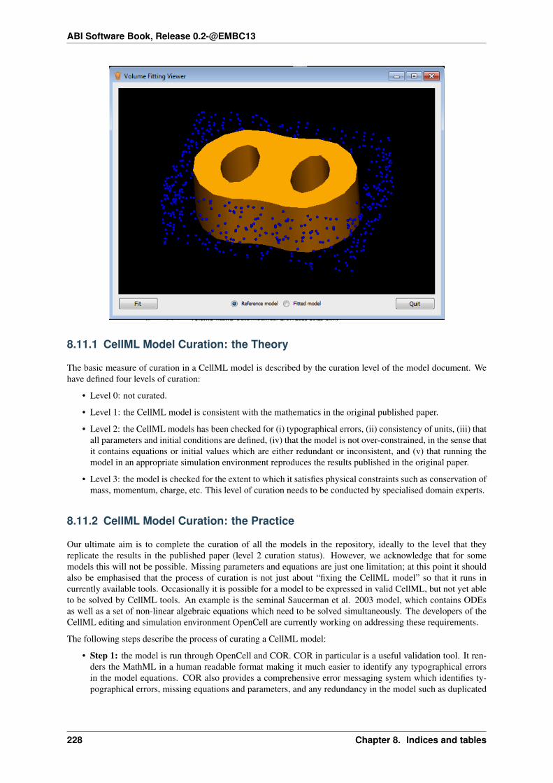
ABI Software Book, Release 0.2-@EMBC13
8.11.1 CellML Model Curation: the Theory
The basic measure of curation in a CellML model is described by the curation level of the model document. Wehave defined four levels of curation:
• Level 0: not curated.
• Level 1: the CellML model is consistent with the mathematics in the original published paper.
• Level 2: the CellML models has been checked for (i) typographical errors, (ii) consistency of units, (iii) thatall parameters and initial conditions are defined, (iv) that the model is not over-constrained, in the sense thatit contains equations or initial values which are either redundant or inconsistent, and (v) that running themodel in an appropriate simulation environment reproduces the results published in the original paper.
• Level 3: the model is checked for the extent to which it satisfies physical constraints such as conservation ofmass, momentum, charge, etc. This level of curation needs to be conducted by specialised domain experts.
8.11.2 CellML Model Curation: the Practice
Our ultimate aim is to complete the curation of all the models in the repository, ideally to the level that theyreplicate the results in the published paper (level 2 curation status). However, we acknowledge that for somemodels this will not be possible. Missing parameters and equations are just one limitation; at this point it shouldalso be emphasised that the process of curation is not just about “fixing the CellML model” so that it runs incurrently available tools. Occasionally it is possible for a model to be expressed in valid CellML, but not yet ableto be solved by CellML tools. An example is the seminal Saucerman et al. 2003 model, which contains ODEsas well as a set of non-linear algebraic equations which need to be solved simultaneously. The developers of theCellML editing and simulation environment OpenCell are currently working on addressing these requirements.
The following steps describe the process of curating a CellML model:
• Step 1: the model is run through OpenCell and COR. COR in particular is a useful validation tool. It ren-ders the MathML in a human readable format making it much easier to identify any typographical errorsin the model equations. COR also provides a comprehensive error messaging system which identifies ty-pographical errors, missing equations and parameters, and any redundancy in the model such as duplicated
228 Chapter 8. Indices and tables

ABI Software Book, Release 0.2-@EMBC13
variables or connections. Once these errors are fixed, and assuming the model is now complete, we com-pare the CellML model equations with those in the published paper, and if they match, the CellML modelis awarded a single star - or level 1 curation status.
• Step 2: Assuming the model is able to run in OpenCell and COR, we then go onto compare the CellMLmodel simulation output from COR and OpenCell with the published results. This is often a case of compar-ing the graphical outputs of the model with the figures in the published paper, and is currently a qualitativeprocess. If the simulation results from the CellML model and the original model match, the CellML modelis awarded a second star - or level 2 curation status.
• Step 3: if, at the end of this process, the CellML model is still missing parameters or equations, or weare unable to match the simulation results with the published paper, we seek help from the original modelauthor. Where possible, we try to obtain the original model code, and this often plays an invaluable role infixing the CellML model.
• Step 4: Sometimes we have been able to engage the original model author further, such that they take overthe responsibility of curating the CellML model themselves. Such models include those published by MikeCooling and Franc Sachse. In these instances the CellML model is awarded a third star - or level 3 curationstatus. While this is laudable, ideally we would like to take the curation process one step further, such thatlevel 3 curation should be performed by a domain expert who is not the author of the original publication(i.e., peer review). This expert would then check the CellML model meets the appropriate constraints andexpectations for a particular type of model.
A point to note is that levels 1 and 2 of the CellML model curation status may be mutually exclusive - in ourexperience, it is rare for a paper describing a model to contain no typographical errors or omissions. In thissituation, Version 1 of a CellML model usually satisfies curation level 1 in that it reflects the model as it is describedin the publication - errors included, while subsequent versions of the CellML model break the requirements formeeting level 1 curation in order to meet the standards of level 2. Taking this idea further, this means that a modelwith 2 yellow stars doesn’t necessarily meet the requirements of level 1 curation but it does meet the requirementsof level 2. Hopefully this conflict will be resolved when we replace the current star system with a more meaningfulset of curation annotations.
Ultimately, we would like to encourage the scientific modeling community - including model authors, journalsand publishing houses - to publish their models in CellML code in the CellML model repository concurrent withthe publication of the printed article. This will eliminate the need for code-to-text-to-code translations and thusavoid many of the errors which are introduced during the translation process.
8.11.3 CellML Model Simulation: the Theory and Practice
As part of the process of model curation, it is important to know what tools were used to simulate (run) the modeland how well the model runs in a specific simulation environment. In this case, the theory and the practice areessentially the same thing, and carry out a series of simulation steps which then translate into a confidence levelas part of a simulator’s metadata for each model. The four confidence levels are defined as:
• Level 0: not curated (no stars);
• Level 1: the model loads and runs in the specified simulation environment (1 star);
• Level 2: the model produces results that are qualitatively similar to those previously published for the model(2 stars);
• Level 3: the model has been quantitatively and rigorously verified as producing identical results to theoriginal published model (3 stars).
8.12 Physiome Model Repository web interface reference
Section author: Dougal Cowan
This document describes the various components of the PMR web interface, which provides access to most of thefunctions of the PMR software via a web browser.
8.12. Physiome Model Repository web interface reference 229

ABI Software Book, Release 0.2-@EMBC13
8.12.1 Physiome Project, CellML, and FieldML views
The Physiome Model Repository can be accessed via three different URLs, each of which gives a specific view ofthe repository:
• http://models.physiomeproject.org - presents an index page that lists the CellML model categories, as wellas a link to a list of FieldML models.
• http://models.cellml.org - presents an index page that only lists the CellML model categories. The pagelogo is the CellML logo instead of the Physiome logo.
• http://models.fieldml.org - presents an index page that lists FieldML models.
Each URL also provides a contextual search. Searching on the FieldML or CellML URLs will only yield FieldMLor CellML results respectively, whereas all model types are included in search results using the Physiome ProjectURL.
8.12.2 Guest view
Browsing the PMR without logging in means you will be restricted to viewing published workspaces only. Brows-ing the repository in this way is only useful for searching, viewing, and downloading published models.
The main navigation bar will only show the Models Home and Exposures buttons.
The search box at the top right hand side of the page can be used to find published workspaces or exposures usingwords such as Author name, physiological or biological terms, or other specific words of interest.
8.12.3 Registered view
Logging in to the repository will provide you with a range of additional functions in the PMR web interface.
An addtional option appears in the navigation bar when you are logged in to the repository site, called MyWorkspaces. Clicking on this will show you a page that lists all of the workspaces you have created on therepository. The page also contains a link to your workspace container, where you can create new workspaces andmanage existing ones.
230 Chapter 8. Indices and tables

ABI Software Book, Release 0.2-@EMBC13
Fig. 8.1: The home page of the PMR when not logged in
Fig. 8.2: The home page of the PMR when logged in as a standard user
8.12. Physiome Model Repository web interface reference 231

ABI Software Book, Release 0.2-@EMBC13
232 Chapter 8. Indices and tables

Index
CClone, 209
EEmbedded workspace, 209Embedded workspaces, 209Exposure, 209Exposures, 209
FFork, 209
MMercurial, 209
PPMR web interface, 14Pull, 209Pulling, 209Push, 209Pushing, 209Python, 209
SSynchronize, 209
WWorkspace, 209Workspaces, 209
233