abbs, charlotte (2014) quantum dynamics of non-linear optomechanical systems. phd...
TRANSCRIPT

Abbs, Charlotte (2014) Quantum dynamics of non-linear optomechanical systems. PhD thesis, University of Nottingham.
Access from the University of Nottingham repository: http://eprints.nottingham.ac.uk/27692/1/C%20Abbs%20PhD%20Thesis.pdf
Copyright and reuse:
The Nottingham ePrints service makes this work by researchers of the University of Nottingham available open access under the following conditions.
This article is made available under the University of Nottingham End User licence and may be reused according to the conditions of the licence. For more details see: http://eprints.nottingham.ac.uk/end_user_agreement.pdf
For more information, please contact [email protected]
Q U A N T U M D Y N A M I C S O F
N O N - L I N E A R O P T O M E C H A N I C A L
S Y S T E M S
by
charlotte abbs , mphys
Thesis submitted to The University of Nottingham
for the degree of Doctor of Philosophy
March 2014


A B S T R A C T
This thesis explores the dynamics of optomechanical systems,
which use radiation pressure to couple together optical and me-
chanical modes. Such systems display dynamics ranging from
the quantum to the classical, with a variety of applications in-
cluding ground state cooling and precision measurements. In
this thesis two different geometries are presented for such a
system in the form of the ‘reflective’ and ‘dispersive’ systems.
Different aspects of the dynamics are investigated numerically
and analytically.
Firstly the reflective system is introduced, which consists of a
cavity formed from a fixed and a moveable mirror. The optical
frequency of the cavity couples linearly to the moveable mir-
ror’s position. This geometry is explored as the cavity is driven
by a laser, revealing a range of dynamical states in the mirror
as the drive frequency is varied.
An alternative geometry is presented in the form of the dis-
persive optomechanical system. Two fixed mirrors with a par-
tially transmitting membrane at the centre provide a cavity
supporting two optical modes, that couple approximately lin-
early or quadratically to the membrane position, depending on
where the membrane is fixed.
The system is explored in both linear and quadratic coupling
regimes. Quadratic coupling is explored for a single optical
mode by selecting a high tunnelling rate through the mem-
brane. The dynamics of the membrane are explored via a simi-
lar set of techniques to those applied to the reflective system.
Linear coupling for two optical modes is explored in the
regimes of blue and red detuning. First resolved sideband cool-
ing is explored, providing an alternative approach ground state
cooling (which has been explored for the reflective case). Fi-
nally, strongly driving the system over a range of coupling
strengths induces classical behaviour, extending from limit cy-
cle oscillations to chaotic motion.
iii


A C K N O W L E D G M E N T S
This thesis would not have been possible without the guidance
and endless patience of my supervisor, Andrew Armour, who
has dedicated so much of his valuable time for discussions and
advice on my project. In addition, I wish to thank my parents,
not only for keeping me alive long enough to finish a PhD,
but for buying me all the study guides, sending me to physics
camp, and giving me those bizarre DOS games that got me
into maths as a child. And to Mr. Campbell and Doug for all
the encouragement.
I would also like to offer my gratitude to a number of other
people who have made my time in Nottingham enjoyable. Firstly
to Luke, my long-suffering partner, for all of his support, and
for generally being the best thing that’s happened to me. I am
grateful for my office friends: Toni, Pete, James, Ben, Lama, Rob,
Jorge and all the theorists - may the Doge be with you, always.
I also acknowledge that without Eric and Joe’s help I might still
be buried in LATEX errors. Also thanks to Fashion Pete, for pro-
viding amusement and hot beverages. Thanks also to the tea
room crew, and all attendees of the Duncan Parkes Memorial
Seminars, for teaching me something new every week.
Thank you, also, to all of the wonderful goths I’ve met since
I moved here - you made me feel welcome from day one. I’d
also like to thank Cheryl and Natalie for teaching me how to
dance my troubles away - you helped me to overcome a disease
which had almost destroyed my life.
And last, but not least, to Cat: mon raison d’etre.
v


C O N T E N T S
1 introduction 1
1.1 Radiation pressure 1
1.2 Optomechanical systems 2
1.3 Applications of optomechanical systems 4
1.4 The structure of this thesis 5
2 the reflective optomechanical system 7
2.1 Introduction 7
2.2 The system 8
2.2.1 Dynamical back-action 9
2.2.2 The Hamiltonian 11
2.2.3 Master equation 12
2.3 Semi-classical approximation 14
2.3.1 Analysis of Langevin equations 17
2.3.2 Damping due to back action 18
2.3.3 Classical dynamics of limit cycles 20
2.3.4 Diffusion 21
2.3.5 Probability distribution 23
2.3.6 Cooling regime 24
2.3.7 Gaussian approximation 26
2.4 Numerical analysis 26
2.4.1 Bad cavity limit 27
2.4.2 Resolved sideband limit 29
2.4.3 Strong coupling regime 31
2.4.4 Comparison of results 33
2.5 Exploring the bistability 35
2.5.1 Calculating the switching rate 37
2.5.2 Relaxation rate calculation 42
2.6 Conclusion 44
3 quadratic coupling in the dispersive system 45
3.1 Introduction 45
3.2 Membrane in the middle system 46
3.2.1 Experimental considerations 47
3.2.2 The Hamiltonian and master equation 48
3.3 Semi-Classical Approximation 51
3.3.1 Analysis of the Langevin equations 52
3.3.2 Damping due to back action 53
3.3.3 Diffusion due to back action 56
vii
viii contents
3.3.4 Probability distribution 57
3.3.5 Cooling Regime 57
3.4 Numerical Analysis 59
3.4.1 Weak coupling 59
3.4.2 Behaviour at strong coupling 61
3.5 Comparison of results 66
3.6 Conclusion 70
4 cooling in a two-mode system 73
4.1 Introduction 73
4.2 The System 74
4.3 Static bistability 77
4.3.1 Routh Hurwitz analysis 81
4.4 Linearized calculation 87
4.4.1 Effective damping 89
4.4.2 Thermal phonon number 94
4.5 Conclusions 97
5 two mode driven dynamics 101
5.1 Introduction 101
5.2 The System 102
5.2.1 Equations of motion for the system 103
5.3 Numerical Analysis 104
5.3.1 Thermally driven system 105
5.3.2 Driven oscillations 106
5.4 Analytic calculation 112
5.4.1 Damping due to Back Action 112
5.4.2 Expressions for cavity variables 113
5.4.3 Solution to Schrodinger equation 115
5.4.4 The Rabi problem 118
5.4.5 Rotating Wave Approximation 120
5.4.6 Limit cycle dynamics 124
5.5 Conclusion 128
a details of wigner transformation 131
b two point correlator for cavity fluctuations 133
c details of numerical calculation 135
d transformation on cavity modes 137
e routh hurwitz stability criterion 141
e.1 Routh array for the static bistability 142

contents ix
f rotating wave approximation for even n 145

L I S T O F F I G U R E S
Figure 1.1 Schematic of reflective and dispersive geometries 3
Figure 1.2 Experimental realisations of mechanical resonators 4
Figure 2.1 Reflective optomechanical system 8
Figure 2.2 Analytic calculation of limit cycles 21
Figure 2.3 Small energy approximation 25
Figure 2.4 Numerical plot of 〈n〉 against ∆ 28
Figure 2.5 Wigner functions of the resonator 29
Figure 2.6 Numerical plots of 〈n〉 and F with respect to λ. 30
Figure 2.7 Plot of 〈n〉 in resolved sideband limit 30
Figure 2.8 Plot of 〈n〉 and F with λ = 2. 31
Figure 2.9 Fano factor in strong coupling regime 32
Figure 2.10 Probability distributions for strong coupling 32
Figure 2.11 Non-classical behaviour in Wigner functions 33
Figure 2.12 Comparison of results in bad cavity limit 34
Figure 2.13 Comparison of probability distributions 35
Figure 2.14 Comparison of results in resolved sideband limit 35
Figure 2.15 Potential barrier for FPT problem 37
Figure 2.16 Eigenvalues of ρ over bistable range 40
Figure 2.17 Comparison of switching rates 41
Figure 2.18 Switching times, calculated analytically 41
Figure 2.19 Comparison of relaxation rates within well 43
Figure 3.1 The dispersive optomechanical system 47
Figure 3.2 Experimental realisation of dispersive geometry 48
Figure 3.3 Damping due to back action 55
Figure 3.4 Small energy approximation 58
Figure 3.5 Numerical plot of 〈n〉 and F with ∆ 60
Figure 3.6 Wigner function at points A, C and D 61
Figure 3.7 Numerical plot of 〈n〉 and F with G 62
Figure 3.8 Fano factor in the strong coupling regime 63
Figure 3.9 Negative Wigner density at strong coupling 63
Figure 3.10 Strong coupling regime 65
Figure 3.11 Comparison of analytic and numerical 〈n〉 and F 67
Figure 3.12 Comparison of limit cycle dynamics 68
Figure 3.13 Comparison of probability distributions 69
Figure 3.14 Comparison of 〈n〉 as G is swept 70
Figure 4.1 Two mode dispersive system 75
Figure 4.2 Mechanical potential function 79
Figure 4.3 Static bistability: Q solutions and frequency shift 80
x

Figure 4.4 Plot of ∆L 80
Figure 4.5 Static bistability for single mode case 83
Figure 4.6 Stability analysis for fixed point solutions 86
Figure 4.7 Damping and frequency shift 93
Figure 4.8 Condition for minimum phonon number 95
Figure 4.9 Minimum effective phonon number 96
Figure 4.10 Plot of Nm 97
Figure 4.11 Plots of Nm at constant ωm 98
Figure 5.1 Two mode driven dispersive system 103
Figure 5.2 Stroboscopic diagrams 108
Figure 5.3 Trajectory of x(t) 108
Figure 5.4 Fixed point dynamics 109
Figure 5.5 Numerically generated limit cycle amplitudes 111
Figure 5.6 The Rabi problem 118
Figure 5.7 Relative error between different γBA calculations 125
Figure 5.8 Comparison of limit cycle predictions 126
Figure 5.9 Approximations used to generate analytics 127
Figure 5.10 Rotating wave approximation 127
Figure E.1 Routh array elements 143
L I S T O F TA B L E S
Table 3.1 Table of parameters. 59
Table 5.1 Parameters for numerical analysis 106
Table E.1 The Routh array. 142
Table E.2 Routh array for static bistability 143
xi


1I N T R O D U C T I O N
Studies of the interaction between light and matter form the ba-
sis of an understanding of how humans observe the world. The
field of quantum optics applies quantum theory to these inter-
actions by accounting for wave-particle duality[1]. That light be-
haves as discrete particles (photons) has been a momentous dis-
covery of the 20th century[2, 3]. Optomechanical systems play
a key role in quantum optics, by coupling optical and mechan-
ical modes together. This coupling allows the behaviour of a
nanoscale object to be observed via measurements of the light
field. Furthermore, optomechanical systems offer insight into a
variety of physical phenomena occurring at the boundary be-
tween quantum and classical physics.
1.1 radiation pressure
A key feature of optomechanical systems is their use of radi-
ation pressure, an effect documented as far back as the 17th
century, when Johannes Kepler noticed that the tails of pass-
ing comets always pointed away from the sun. This led him
to postulate the existence of a ‘solar breeze’, blowing the tails
outwards from the sun[4]. This was accompanied by an appeal
that “ships and sails proper for heavenly air should be fash-
ioned” so that humans could travel the skies. Unwittingly, he
had stumbled upon the concept of solar sails - a feat of en-
gineering which has recently been achieved by the Japanese
Aerospace Exploration Agency[5].
What Kepler had actually observed was the action of radi-
ation pressure on the tails of comets. Solar photons strike the
vapourized gas particles emitted from the comet, and scatter off
them. The change in their momentum results in a force on the
gas, in the photon’s original direction of travel. The effect oc-
curs when photons strike any surface, but is more pronounced
for a reflecting body, where the change in momentum is twice
the original momentum. The force F exerted on a completely re-
flecting surface by a light beam of power P is F = 2P/c, where
c is the speed of light.
1

2 introduction
Long after Kepler, the existence of radiation pressure was
verified in laboratory conditions by Lebedev in 1901[6]. Owing
to the small momentum carried by photons, the pressure force
is typically too small to deflect a macroscopic object. However,
the effect can be magnified by selecting lightweight, reflecting
objects with large surface areas, and using high intensity light.
This is the principle behind the design of solar sails[7, 8]; these
large, reflecting sheets of metal are propelled through space
using only the radiation emitted from the sun.
1.2 optomechanical systems
In order to observe deflection of objects by light much closer to
home, optomechanical systems have been developed. A cavity
formed from two mirrors, driven by a laser, provides a practical
system in which to observe the effects of radiation pressure, as
the force is amplified by repeated reflections. The light field cir-
culating the cavity is coupled to a mechanical mode, provided
by a resonator of some description. The simplest example is
a setup where one of the cavity mirrors is mounted on a can-
tilever, which is free to move along the cavity’s axis. Figure 1.1a
shows such a system. Light striking the mirror then causes a de-
flection, altering the length of the cavity, and changing the fre-
quency of the circulating radiation. This is the reflective setup,
and provides a scenario where the optical frequency is coupled
linearly to the position of the cantilever. An example of a me-
chanical mirror is given in Figure 1.2a.
The interplay of forces within the system results in a variety
of dynamical effects, depending on how it is driven. As radia-
tion circulates the cavity, a radiation pressure force is exerted
on the mechanical element. The optical frequency changes as
the mirror moves in response to the force, altering the intensity
of radiation. However, radiation takes a finite time to leak out
of the cavity. As a result the cavity responds to the mirror’s
motion with a time lag, and an effect known as back action
arises, whereby the radiation force acts back on the resonator
as it moves[9]. This effect can be used to either put energy into
the resonator or extract it.
Varying the coupling strength allows one to observe a range
of states in the resonator, from the classical to the quantum[10,
11, 12]. Driving the cavity below resonance extracts energy from
the resonator, allowing it to be cooled to its quantum ground
state[13, 14]. When the cavity is driven above resonance, one

1.2 optomechanical systems 3
q(t)
i
rFrad
M1 M2
C
L
q(t)
M2M1
D
tL
(a) (b)
i
r
X
Figure 1.1: Schematic diagrams of different examples of optomechan-
ical geometries: (a) the reflective system, consisting of a
cavity formed by a fixed mirror M1 and a movable mirror
M2, mounted on a cantilever, C, and free to move along
the cavity’s axis. (b) The dispersive system, where the cav-
ity is formed from two fixed mirrors, M1 and M2. The
mechanical mode is provided by a membrane, D, which
is clamped at X, free to move along the cavity’s axis. Both
are driven by laser radiation, L, with mechanical displace-
ment measured by q(t).
can observe a situation where energy is absorbed by the res-
onator, creating phonons. The motion of the resonator can be
characterised by two quantities; the damping due to back action
and the phase diffusion in the resonator’s state. Another useful
quantity to define is the Fano factor - this measures the spread
in the distribution of phonons present in the resonator, which
depends on both the damping and diffusion. One of the first
signifiers of quantum behaviour is when the Fano factor drops
below unity, indicating number squeezing in the mechanical
mode[10, 12, 15].
In recent years alternative ways of combining optical and me-
chanical modes have been explored. In this thesis, one such al-
ternative geometry is explored in detail. This is often referred to
as ‘dispersive optomechanics’[16], an example is shown in Fig-
ure 1.1b. For this geometry, both cavity mirrors are fixed, and
the mechanical element takes the form of a partially transmit-
ting membrane mounted on a cantilever at the centre of the
cavity. Figure 1.2b shows an example of a membrane made
from silicon nitride. This has the advantage of offering either

4 introduction
linear or quadratic coupling between the mechanical and opti-
cal modes, depending on the positioning of the resonator[17].
Additional advantages are apparent when considering the
engineering of such systems experimentally. The reflective setup
requires the fabrication of mechanical elements with both a
high quality factor and a highly reflecting surface[18]. Practi-
cally speaking this has proven difficult. By choosing a system
with two fixed reflecting surfaces and a separate membrane
with the high quality factor, one does not require these two
properties to be combined in a single structure. For experiments
in dispersive optomechanics, membranes are generally fabri-
cated from high-stress stoichiometric silicon nitride[18]; this
provides a material with low intrinsic losses[19] and minimal
optical absorption[20] - providing high mechanical quality fac-
tors and optical finesses simultaneously. An example of such a
membrane is give in Figure 1.2b. Here the 50 nm thick Silicon
Nitride is mounted on a Silicon microchip.
20µm
(a) (b)
Figure 1.2: Experimental realisations of resonators for (a) the reflec-
tive system and (b) the dispersive system. The example
in (a) is adapted from [21], and shows a suspended mi-
croscale mirror. In (b) a silicon nitride membrane, of di-
mensions 1mm × 1mm × 50nm, is mounted on a silicon
chip, and is adapted from [22].
1.3 applications of optomechanical systems
The applications of optomechanical systems are manifold. Op-
tomechanical systems allow one to probe physical effects which
lie along the boundary between quantum and classical physics.
Whilst the scale of a mechanical resonator can be as large as
centimetres, theoretical work suggests that strong coupling to
the light field may allow quantum effects to be observed on a
relatively large scale. These include superposition[11], decohe-
rence [23], squeezing[10] and entanglement[24]. Depending on

1.4 the structure of this thesis 5
the type of coupling, one may also be able to make quantum
non-demolition (QND) measurements of the light field[7], as
well as precision measurements on the resonator state. In the
case of linear coupling, one can measure the position of the res-
onator by monitoring the light field leaking out of the cavity.
In the case of quadratic coupling, the energy of the mechani-
cal component can, in principle, be measured, thus providing a
possible way of observing quantization of energy[25].
Optomechanics has been at the centre of the development
of gravitational wave detectors. For a number of years, experi-
ments aimed at the detection of gravitational waves have made
use of interferometers with mechanically suspended mirrors[7,
8]. For these large scale optomechanical systems, the effects of
back action were undesirable. Since the initial experiments of
the 1970s and 1980s, however, the effects of back action have
generated much interest, with experiments emerging to study
it on a smaller scale.
There exist many variations on the optical cavity system -
all with the central feature of a resonance which is tuned by
mechanical motion, and experiences a delayed response. The
resonance can be provided by an optical mode or an electro-
magnetic resonance. Examples include the optical cavity dis-
cussed, whispering gallery modes[26], single electron transis-
tors (SETs)[15] and superconducting LC-circuits[14]. The me-
chanical element can be provided by anything from a cantilever
[27] - in the case of a cavity mirror - to a movable capacitor
plate[15] - in the case of the SET and can range in scale from
nanometres [28] (in the setup discussed) to centimetres[29] (in
the case of gravitational wave detectors).
1.4 the structure of this thesis
This thesis is organised as follows. Chapters 2 introduces the
reflective optomechanical system, providing a description of a
linearly coupled optomechanical system. The central features
of the system are presented, and some analytic techniques in-
troduced, which will be utilised in further chapters. A Wigner
transformation is presented, which allows one to model certain
aspects of the system analytically, under certain circumstances.
In addition, several features are explored numerically by solv-
ing the master equation. This allows a contrast to be drawn
between the classical and quantum regimes as the optomechan-
ical coupling is swept. In addition, the limits of the Wigner

6 introduction
transformation are tested by calculating the switching rate for
a bistable state.
Chapter 3 introduces the dispersive optomechanical system.
This kind of system offers an alternative method of exploring
optomechanical coupling, without the fabrication problems pre-
sented by the reflective system. Parameters in this chapter are
selected to produce quadratic coupling between a single opti-
cal and mechanical mode. A similar analysis to Chapter 2 is
then applied to describe the system analytically. Comparing
this with a similar numerical calculation, the applicability of
the Wigner transformation can be compared for the reflective
and dispersive different systems. Additional numerical analy-
sis explores quantum features of the dispersive system in the
strong coupling regime.
Chapter 4 examines the dispersive optomechanical system, in
the regime where two optical modes are important. Here the re-
gime of red detuning is explored, with the aim of investigating
the extent to which the system can be used to cool the resonator
to its quantum ground state. Such a feat has been achieved us-
ing the reflective system[13, 14], but further advances would be
needed to achieve this using the more easily fabricated disper-
sive system.
Chapter 5 explores the dispersive system further, in the re-
gime of blue detuning. Here strong coupling drives the res-
onator into a state of self-oscillation, where dynamical multi-
stability is possible. In this regime, fluctuations are neglected
and a semi-classical approach can be taken to investigate the
dynamics. The dynamics are mapped out numerically, over a
range of couplings, before an analytic approximation is applied
to predict the amplitudes of limit cycle oscillations.
The results of Chapter 2, Sections 2.3 and 2.4 comprise prior
work on the truncated Wigner approach to optomechanical sys-
tems, by Denzil Rodrigues and Andrew Armour. These results
have been published in [15, 30, 31]. The results of Chapter 2,
Section 2.5 and Chapters 3 to 5 contain original research under-
taken in collaboration with Andrew Armour.

2E X P L O R I N G T H E R E F L E C T I V E
O P T O M E C H A N I C A L S Y S T E M
2.1 introduction
This chapter presents an in depth analysis of the reflective op-
tomechanical system. This couples the optical resonance of a
cavity to the mechanical motion of a suspended mirror, pro-
viding an example of linear coupling between position and fre-
quency. The cavity mode is driven by radiation from a laser
source. The circulation of radiation within the cavity results in
an energy exchange between the optical and mechanical modes.
The driving frequency determines the type of exchange; driv-
ing above resonance (blue detuning) causes energy to be trans-
ferred to the resonator whilst driving below resonance (red de-
tuning) results in energy being extracted from the resonator.
Since the optical frequency couples linearly to the mechani-
cal displacement, an accurate measurement of the resonator’s
position is possible via measurement of the cavity frequency.
This opens up the possibility of precision measurements of such
objects to within their ground state uncertainty[32]. For such
measurements, the effects of ‘back action’ can be undesirable
due to photon shot noise[33] which causes fluctuations in the
mechanical position. Increasingly, research into optomechanical
systems has utilised the effects of back action for the purposes
of ground state cooling of resonators[34, 35, 36, 13]. This has
led to the achievement of quantum ground state cooling in the
reflective optomechanical system[14].
Recently, however, research has also begun to explore the re-
gime of blue detuning[37, 38, 39]. In this regime the mechani-
cal mode can be driven into a regime of self-oscillations where
losses are balanced by radiation forces[9, 40]. Effects such as
dynamical multistability[41] and chaos[42] result from strong
driving. More recently, the regime of strong coupling has been
explored in both theory[10, 43] and experiment[44], with the
aim of generating non-classical states in the resonator, includ-
ing squeezed states[45] and entangled states[24].
This chapter explores linear coupling in both the blue and red
detuned regimes, by introducing the reflective optomechanical
7

8 the reflective optomechanical system
system in Section 2.2. The optical mode is assumed to be driven
at a range of frequencies and the response of the resonator in-
vestigated both analytically and numerically. In Section 2.3 the
dynamics are explored analytically via a semi-classical approx-
imation, which applies in the weak coupling regime. In Sec-
tion 2.4 a numerical approach is taken, by solving the master
equation. The resonator dynamics are investigated by tuning
the drive frequency. The average phonon number and Fano
factor are plotted, revealing transitions between stable states,
observed in the Wigner function. Numerical results are then
compared to plots generated using the analytic approximation
of Section 2.3. Finally, a bistable regime is explored in Section
2.5 and a semi-classical calculation of the switching rate is com-
pared to a fully quantum one.
2.2 the system
L
q(t)
cavity mode, ω0
i
r Fradlaser
q = 0
(a)
ω′0 ωd
na
(i) (ii)
(b)
Figure 2.1: Reflective setup for an optomechanical system (a)
schematic diagram showing a cavity formed from two
mirrors spaced by distance L, one of which is mounted
on a mechanical cantilever at position q = 0. As the cav-
ity mode, ω0, is driven by a laser, radiation circulates in
the cavity and produces a pressure force Frad on the can-
tilever as an incident wave (i) which is reflected (r). This
results in a displacement q(t), which alters the optical cav-
ity frequency, from ω0 to ω′0. The number of photons, na,
responds to the driving frequency, ωd, as shown in (b).
Points [i] and [ii] indicate regions where the drive fre-
quency results in damping and driving, respectively.

2.2 the system 9
Consider the system shown in Figure 2.1a. A cavity is formed
from two mirrors. One mirror is mounted on a mechanical
resonator (eg a cantilever), allowing it to move along the axis
shown by the dotted line. The position of the resonator is given
by q(t). With q = 0 the cavity supports optical modes, of fre-
quency ω0, determined by the cavity length, L:
ω0 =2kπc
L, (2.1)
where c is the speed of light and k is an integer denoting which
order of resonance is being probed. A laser drives the cavity
near its resonant frequency, radiation circulates within the cav-
ity, exerting a radiation pressure on the movable mirror[46, 6].
This causes a deflection in the mirror, altering the cavity length
and thus the frequency as
ω′0(t) =2kπc
L + q(t)(2.2)
≈ ω0 −ω0
Lq(t). (2.3)
In this way the optical frequency couples linearly to the posi-
tion of the mechanical mode[30, 17]. The coupling strength is
denoted λ0,
λ0 = −ω0
L. (2.4)
This is known as the ‘reflective’ setup, as the radiation is re-
flected by the mechanical element.
2.2.1 Dynamical back-action
The mechanical element is displaced via a radiation pressure
force, caused by photons striking it. The total force is thus di-
rectly proportional to the number of photons in the cavity at a
given time, na(t). A classical equation of motion can be written
for a resonator of mass m and natural frequency ωm:
mq + γq + mω2mq = F0na(t), (2.5)
where γ is the intrinsic damping of the resonator and F0 is the
force exerted by each photon. The displacement of the mirror
alters the frequency of the optical mode, whilst the drive fre-
quency remains constant. As a result the number of photons in
the cavity changes,
na(t) ≈ n0(t) +dna
dqq(t), (2.6)

10 the reflective optomechanical system
where n0(t) is the number of photons circulating when q(t) = 0.
The damping constant for the cavity is given by κ, and this de-
termines the timescale over which photons leak out. As a result
there is a finite ‘ring down’ time[9], resulting in a delayed re-
sponse to the mechanical motion, causing a time lag between
the resonator being displaced and the photon intensity chang-
ing. This means that na(t) actually depends on q(t− τ), where
τ = κ−1.
na(t) ≈ n0(t) +dna
dqq(t− τ) (2.7)
≈ n0(t) +dna
dq(q(t)− τq) (2.8)
Since the photon intensity affects the radiation pressure, the
force on the mechanical mode also responds with a time lag,
and Equation 2.5 becomes
mq +
(
γ + F0τdna
dq
)
q + m
(
ω2m −
F0
m
dna
dq
)
q = F0n0(t). (2.9)
From Equation 2.9, the effect of the optomechanical coupling to
na has three identifiable results, a static shift in the equilibrium
position of q, determined by n0, a modification to the damping
and a frequency shift, both proportional to dna/dq. Since the
position modulates the optical frequency, this can be written
dna
dq=
dω′0dq
dna
dω′0. (2.10)
Figure 2.1b illustrates the cavity response to the drive frequency,
in terms of the photon number. The graph takes the form of a
Lorentzian curve[9], peaked around ω′0 (which changes with q).
The quantity dω′0/dq is determined by the geometry of the
system. For the system shown in Figure 2.1a, dω′0/dq < 0. Fig-
ure 2.1b illustrates the cavity’s response to the optical drive pro-
vided by the laser source. As ωd approaches ω0, the number of
photons circulating in the cavity increases rapidly, so that a res-
onance occurs at ωd = ω0. Two different scenarios of detuning
are labelled (i) and (ii) in Figure 2.1b:
[i ]When the system is driven below resonance (red detun-
ing), a decrease in ω′0 brings the system closer to reso-
nance, such that dna/dω′0 < 0. As a result, dna/dq > 0,
so that the system is more heavily damped. In addition,
the effective mechanical frequency is reduced.

2.2 the system 11
[ii ]When the system is driven above resonance (blue detun-
ing), an increase in ω′0 brings the system closer to reso-
nance, such that dna/dω′0 > 0. As a result, dna/dq < 0,
so that the total damping in the system is reduced and
the mechanical frequency increased.
The resulting forces on the resonator in response to its mo-
tion are referred to as dynamical ‘back action’. This effect can
be used to cool or drive a resonator[36, 31]. This thesis will ad-
dress both of these cases, in various optomechanical systems.
The present chapter focuses largely on the case of blue detun-
ing, with the case of red detuning briefly addressed in Section
2.3.6.
2.2.2 The Hamiltonian
The system of Figure 2.1a is now analysed in detail. Consider
an optical mode with frequency ω0, driven by a laser with fre-
quency ωd, which is coupled by radiation pressure to a mechan-
ical mode of frequency ωm. Provided ω0 ≫ ωm, the Hamilto-
nian of the system can be written in the form[35]
H = ω0a†a + ωmb†b + λ(
b + b†)
a†a
+Ω(
ae−iωdt + a†eiωdt)
, (2.11)
where a and b are annihilation operators for the optical and me-
chanical modes, respectively and Ω is the strength of the laser
drive. The mechanical mode has natural frequency ωm and is
coupled with strength λ to the optical mode, which relates to
λ0 by
λ =λ0√2mω
. (2.12)
The units are chosen so that h = 1, this will be the case for
the entire thesis. The term in λ is the coupling between the
two harmonic oscillators, and is the source of the non-linear
behaviour in the system.
To remove the explicit time dependence in the Hamiltonian,
one can transform into a frame rotating at the drive frequency.
A unitary transformation, U = eiH0t is performed on H, giving
H = UHU† with H0 = ωda†a. This results in a transformed
Hamiltonian of the form
H = ω0a†a + ωmb†b + λ(
b + b†)
a†a + Ω(
a + a†)
. (2.13)

12 the reflective optomechanical system
To obtain the effective Hamiltonian, which acts on the trans-
formed wavefunction, |ψ′〉 = U|ψ〉, consider the Schrodinger
equation acting on the wavefunction, |ψ〉:
i∂|ψ〉
∂t= H|ψ〉. (2.14)
The transformed wavefunction, |ψ′〉 must obey the same equa-
tion, with H = He f f . This leads to an effective Hamiltonian
He f f = H − H0, thus
He f f = ∆a†a + ωmb†b + λ(
b + b†)
a†a + Ω(
a + a†)
, (2.15)
where ∆ = ω0 −ωd is the detuning of the laser drive.
2.2.3 Master equation
The Hamiltonian of Equation 2.15 captures the dynamics of an
isolated optomechanical system, however this is not a realistic
scenario. In practice any systems fabricated experience dissipa-
tion, reducing the cavity finesse, F , and mechanical quality fac-
tor, Q. The master equation includes losses in the system which
lead to damping and decoherence in the cavity and resonator
modes, by modelling the effects of coupling the system to its
environment.
One can model the losses in the cavity by coupling the opti-
cal mode to a spectrum of modes outside of the cavity, which
describe its environment. The origin of losses in the resonator
is less well understood. Prior investigations propose dissipa-
tion due to clamping losses via the cantilever supports[47] as
well as defects in the resonator’s structure[48]. For the follow-
ing analysis, a simple model for the dissipation in the optical
and mechanical modes will be used. This is often applied in
the field of optomechanics[49]. Both modes are coupled to heat
baths describing their environments, which consist of a series of
harmonic oscillators - optical modes for the cavity and phonon
modes for the resonator, which describe the bulk material the
cantilever is clamped to.
With these assumptions an effective master equation can be
written down[1], describing the evolution of the reduced den-
sity matrix for the system:
ρ = −i [H, ρ] + Laρ + Lbρ, (2.16)
2.2 the system 13
where La and Lb are operators describing the dissipation from
the cavity and resonator, respectively, they are given by
Laρ = −κ
2(na + 1)
(
a†aρ + ρa†a− 2a†ρa)
−κ
2na
(
aa†ρ + ρaa†−2aρa†)
, (2.17)
Lbρ = −γ
2(n + 1)
(
b†bρ + ρb†b− 2b†ρb)
−γ
2n(
bb†ρ + ρbb† − 2bρb†)
, (2.18)
where na and n describe the thermal occupation of the cavity
and resonator, respectively and are determined by their temper-
ature T:
na =[
eω0/kBT − 1]−1
, (2.19)
n =[
eωm/kBT − 1]−1
, (2.20)
where kB is Boltzmann’s constant. The dissipation terms of
Equations 2.17 and 2.18 do not account for the coupling be-
tween the mechanical and optical modes, but this is a higher
order effect[49], and is ignored when considering the weak cou-
pling modelled in this system.
The transformation detailed in Equations 2.13 to 2.15 does
not affect the dissipation terms. As a result Equation 2.16 can be
transformed to describe the density matrix in the frame rotating
at the drive frequency. This matrix is denoted ρ and obeys a
master equation of the form
˙ρ = −i[
He f f , ρ]
+ Laρ + Lbρ. (2.21)
The cavity is assumed to have na = 0. Because of the high
optical frequency, its thermal occupation remains negligible up
to Ta ∼ 300K.
At this point two approaches can be taken. The aim is to in-
vestigate the mechanical mode, and determine the behaviour
of the resonator within the coupled system. It is possible to do
this both analytically and numerically. A numerical approach
entails solving the master equation directly to get ρ, the den-
sity matrix (as described in Section 2.4). This encodes the prop-
erties of the resonator, which allows one to calculate its average
properties, given
〈O〉 = Tr[
ρO]
, (2.22)

14 the reflective optomechanical system
for any observable operator, O. An alternative route (described
in Section 2.3) involves a semi-classical approximation, which
describes the approximate behaviour of the system within a
certain range of parameters.
2.3 semi-classical approximation
An analytic approach describes the dynamics of the system in
the weak coupling regime, using a semi-classical approxima-
tion [30, 1]. The calculation proceeds via a Wigner transforma-
tion, whereby complex numbers α and β are introduced to de-
scribe the phase space of the cavity and resonator, respectively[1].
The Wigner function is a quasi probability distribution used
in quantum mechanics[1, 50]. For a given wave function, it is
a generating function for all spatial auto-correlation functions,
encoding all the quantum expectation values for a given density
matrix[51]. For the cavity-resonator system it is written as the
Fourier transform of the characteristic function of the density
operator,
W(α, β) =1
π2
∫
d2ηa
∫
d2ηb eη∗a α−ηaα∗eη∗b β−ηbβ∗χ (η1, η2) ,(2.23)
where the characteristic function, χ(η1, η2) uniquely defines the
density operator, and is given by[1]
χ (η1, η2) = Tr[
ρeηaa†−η∗a aeηbb†−η∗b b]
. (2.24)
The phase space variables α and β replace the quantum op-
erators, a and b. The two sets of variables are related by their
averages, thus for example
〈α∗α〉 ⇐⇒ 1
2〈a†a + aa†〉 (2.25)
〈β∗β〉 ⇐⇒ 1
2〈b†b + bb†〉, (2.26)
where averages are taken over the distribution of states in the
system.
In quantum mechanics the Wigner function plays an analo-
gous role to the classical probability distribution. However, it
also accounts for the uncertainty principle and includes quan-
tum features, thereby failing to satisfy certain criteria which
apply to probability distributions[52]. For instance, it may take
on negative values[10, 12].

2.3 semi-classical approximation 15
A Wigner transformation on the master equation (Equation
2.21) gives
∂W
∂t=
∂
∂β∗
(
−iωmβ∗ − iλ
(
α∗α− 1
2
)
+γ
2β∗)
W
+∂
∂β
(
iωmβ + iλ
(
α∗α− 1
2
)
+γ
2β
)
W
+∂
∂α∗
(
−i∆α∗ − iλ(β + β∗)(
α∗α− 1
2
)
+κ
2α∗)
W
+∂
∂α
(
i∆α + iλ(β + β∗)(
α∗α− 1
2
)
+κ
2α
)
W
+κ
2
∂2W
∂α∂α∗+
γ
2(n + 1)
∂2W
∂β∂β∗
+iλ
8
(
∂3W
∂β∂α∂α∗− ∂3W
∂β∗∂α∂α∗
)
, (2.27)
where the shorthand W = W(α, β) is used for the Wigner func-
tion. Details for the calculation are supplied in Appendix A.
This transformation is exact and describes the full quantum be-
haviour of the system.
The third order derivatives present a problem, however. If it
weren’t for their presence the equation would be in the form of
a Fokker-Planck equation. This would allow equations of mo-
tion to be written as a set of coupled Langevin equations[1, 50].
There are two possible solutions to this conundrum. Firstly, a
different transformation is possible using the Positive-P distri-
bution [1, 53]. This does not involve third order terms and so
a Fokker-Planck type equation is obtained. Unfortunately the
transformation is much more complicated, and the phase space
required is twice as large[1]. In this instance, the truncated Wig-
ner approximation (TWA) is applied. This involves simply drop-
ping the third order derivatives in Equation 2.27. The equation
then accounts for the zero point noise in the system, but does
not treat the non-linearity exactly[54]. This approximation is
known to work in the case of systems close to a steady state,
with linear fluctuations[1]. This requires λ to be kept small so
that interactions between the cavity and resonator are relatively
weak. Quantitatively, it is required that λ≪ 2ωm[31].

16 the reflective optomechanical system
The approximated Fokker-Planck equation takes the form
dW(α, β)
dt=
∂
∂α[Fα(α, β)W(α, β)] +
∂
∂α∗[Fα∗(α, β)W(α, β)]
+∂
∂β
[
Fβ(α, β)W(α, β)]
+∂
∂β∗[
Fβ∗(α, β)W(α, β)]
+1
2
∂2
∂β∂β∗[
Dβ(α, β)W(α, β)]
+1
2
∂2
∂α∂α∗[Dα(α, β)W(α, β)] , (2.28)
where the following functions are defined:
Fα = i∆α + iλ(β + β∗)(
α∗α− 1
2
)
+κ
2α + iΩ (2.29)
Fα∗ = (Fα)∗ (2.30)
Fβ = iωmβ + iλ
(
α∗α− 1
2
)
+γ
2β (2.31)
Fβ∗ =(
Fβ
)∗(2.32)
Dα = κ (2.33)
Dβ = γ(n + 1), (2.34)
where Fα,β describe the forces acting on the system, and Dα,β
describe the diffusion in the system. This can be written in the
equivalent form of a set of Langevin equations for variables α,
α∗, β and β∗[1],
α = −i
(
∆ +λ
2(β + β∗)
)
α− κ
2α− iΩ + ηα (2.35)
α∗ = i
(
∆ +λ
2(β + β∗)
)
α∗ − κ
2α∗ + iΩ + ηα∗ (2.36)
β = − iλ
2
(
α∗α− 1
2
)
− iωmβ− γ
2β + ηβ, (2.37)
β∗ =iλ
2
(
α∗α− 1
2
)
+ iωmβ− γ
2β + ηβ∗ , (2.38)
where fluctuations in the cavity and resonator are described by
Gaussian white noise variables ηα and ηβ, respectively. These
noise terms are governed by the following correlators:
〈ηα(t)ηα∗(t′)〉 =
κ
2δ(t− t′), (2.39)
〈ηβ(t)ηβ∗(t′)〉 =
γ
2(2n + 1)δ(t− t′). (2.40)
All other correlators are zero. Equations 2.35 to 2.38 are cou-
pled, non-linear equations, which cannot be solved exactly. In

2.3 semi-classical approximation 17
the following, solutions are derived via a series of approxima-
tions, consistent with a weakly coupled system, where λ ≪2ωm.
2.3.1 Analysis of Langevin equations
Analysis of the resonator dynamics requires a decoupled equa-
tion for β. In order to proceed, additional approximations are
required. Equations 2.35 to 2.38 are analysed by exploiting the
separation of time-scales in the cavity and resonator dynam-
ics. The damping in the cavity determines the time-scale over
which oscillations in the optical mode relax, and is significantly
higher than both the mechanical damping and the coupling be-
tween the modes: κ ≫ γ, λ. The cavity therefore loses energy
via dissipation on a much faster timescale than energy is trans-
ferred to or lost from the resonator, and over the timescale of
cavity relaxation, any variations in the mechanical amplitude
are small. One can therefore describe the cavity dynamics with
respect to a mechanical mode which oscillates at a fixed fre-
quency with a constant amplitude[41]. This amounts to the
ansatz β = βc + Be−iφe−iωmt, where φ and B are treated as con-
stants, and βc is a constant shift in the origin of the resonator,
which is yet to be evaluated. Equation 2.35 then reads
α = −i(
∆′ + λB cos (φ + ωmt))
α− iΩ− κ
2α + ηα,(2.41)
where ∆′ = ∆ + λℜ[βc] is the detuning including a frequency
shift brought about by the fixed point displacement of the res-
onator, βc. By making a further substitution, α = αeiz sin (φ+ωmt),
where z = λBωm
, one can isolate the oscillating terms in the rotat-
ing frame of α,
dα
dt= −i∆′α− iΩeiz sin (φ+ωmt) − κ
2α + ηα, (2.42)
where ηα = ηαeiz sin (φ+ωmt).
After a Fourier Transform and some rearranging, a solution
for α(ω) takes the form
α(ω) =−iΩ
i(ω + ∆′) + κ2
∫ ∞
−∞dt′e−i(ωt′−z sin (ωmt′)−ωφ/ωm)
+ηα(ω)
i(ω + ∆′) + κ2
. (2.43)

18 the reflective optomechanical system
By applying the Jacobi-Anger expansion[55], the integral is eval-
uated,
α(ω) =−iΩ ∑n Jn(z)eiφn
κ2 + i(ω + ∆′)
δ(ω + ωmn) +ηα(ω)
κ2 + i(ω + ∆′)
, (2.44)
where ∑n Jn(z) denotes a sum over bessel functions of the first
kind, Jn(z), over the limits n = −∞ to n = ∞. The first term in
Equation 2.44 can be identified as an average, 〈α〉, and the sec-
ond as the fluctuating part, δα. A similar expression is derived
for α∗, where α∗(ω) = α∗(ω)e−iz sin (φ+ωmt):
α∗(ω) =iΩ ∑n Jn(z)e−iφn
κ2 + i(ω− ∆′)
δ(ω + ωmn) +η∗α(ω)
κ2 + i(ω− ∆′)
. (2.45)
Note that, after a Fourier transform, α∗(ω) and α(ω) are no
longer complex conjugates of one another.
2.3.2 Damping due to back action
Turning now to Equation 2.37, analysis of the mechanical mode
requires one to evaluate the term α∗α − 1/2. In order to so,
recall the assumptions made when applying the TWA. In drop-
ping the third order differentials, an accurate picture of the
zero-point noise in the system is acquired, at the cost of describ-
ing the non-linearity exactly. This works well when fluctuations
are weak, and so one can write α = 〈α〉+ δα, and approximate
δαδα∗ by its average, 〈δαδα∗〉 = 12 . Doing this (as described in
Appendix B), one finds
α∗α− 1
2= 〈α∗〉〈α〉+ 〈α〉δα∗ + 〈α∗〉δα, (2.46)
This term describes the resonator dynamics arising from the
coupling to the cavity mode. It is composed of an average and
fluctuating dynamics, which can be treated separately. Turn-
ing attention to the average dynamics, the resonator amplitude
evolves according to
〈β〉 = −(
iωm +γ
2
)
〈β〉 − iλ
2〈α∗〉〈α〉. (2.47)
The last term in Equation 2.47 can be evaluated via a Fourier
transform,
〈α∗〉〈α〉(ω) = Ω2 ∑n,n′
Jn(z)Jn′(z)δ ( fn,n′(ω)) e−iφ(n−n′)
h∗n(hn + iω), (2.48)

2.3 semi-classical approximation 19
where it has been noted that 〈α∗〉〈α〉(ω) = 〈α∗〉〈α〉(ω), and the
quantities hn and f (ω) have been defined:
hn =κ
2+ i(ωmn + ∆′) (2.49)
fn,n′(ω) = ω + ωm(n− n′). (2.50)
Analysis of the centre of the limit cycle, βc is immediately pos-
sible, by isolating the non rotating terms in Equation 2.47,
βc = −iλ
2
〈α∗〉〈α〉(ω = 0)
iωm + γ2
, (2.51)
where 〈α∗〉〈α〉(ω = 0) denotes the non rotating term in the
sum of Equation 2.48. When ω = 0 the delta function isolates
the term n′ = n in the sum over n′ to give
βc = − λΩ2
2ωm − iγ ∑n
J2n(z)
κ2
4 + (ωmn + ∆′)2. (2.52)
Switching attention, now, to the oscillating parts of Equation
2.47, a rotating wave approximation[56] (RWA) is applied. This
isolates terms in the sum of Equation 2.48 that oscillate near
the mechanical frequency, since higher frequency oscillations
at nωm (where n > 1) will produce negligible contributions
when the average is taken over a long enough timescale. These
terms are therefore discarded so that Equation 2.53 can then be
written
〈β〉 = −i (ωm + δω) 〈β〉 − 1
2(γ + γBA) 〈β〉, (2.53)
where the damping due to the cavity back action, γBA, and
frequency shift, δω, are identified as the real and imaginary
parts of the truncated sum in Equation 2.48. The discarding of
higher order oscillations in ωm amounts to picking out terms
in the sum where n′ − n = 1, giving
γBA
2+ iδω = − iλΩ2
2B
∑n Jn(z)Jn+1(z)
h∗nhn+1. (2.54)
Taking the real and imaginary parts, the damping and fre-
quency shift are then expressed in terms of z,
γBA(z) = −∑n
λ2Ω2κ
2z
Jn(z)Jn+1(z)
|hn|2|hn+1|2(2.55)
δω(z) = ∑n
λ2Ω2
2ωmz
Jn(z)Jn+1(z)
|hn|2|hn+1|2. (2.56)

20 the reflective optomechanical system
These two expressions are thus amplitude dependent, a prop-
erty which will be investigated in later sections. It should be
noted that the approximation in making the ansatz β = βc +Be−i(ωmt+φ) neglects variations in frequency, which are then cal-
culated in the form of δω(z). The calculation is not done self
consistently as δω(z) is found to be several orders of magnitude
smaller than ωm for the parameters of interest. This results in
relative errors of around 10−5 when calculating γBA(z), and so
the correction is ignored.
2.3.3 Classical dynamics of limit cycles
Equation 2.53 describes the average dynamics of the resonator,
leading to a classical equation of motion for the amplitude B:
〈B〉 = −γT(B)
2〈B〉, (2.57)
where the total damping is written γT(B) = γ + γBA(B). Two
types of steady state solution, B0, are possible to satisfy Equa-
tion 2.57:
(i) B0 = 0: a ‘fixed point’ state, where the resonator fluctuates
around a central point, βc.
(ii) B0 6= 0: a ‘limit cycle’ state, where the resonator oscillates
with a constant amplitude about βc.
Both of these obey the condition
(γ + γBA(B0)) B0 = 0. (2.58)
Note that B0 = 0, the state corresponding to a fixed point, is al-
ways a solution (though not necessarily a stable one). One can
obtain solutions for limit cycles, B0 6= 0, for a given set of pa-
rameters by finding the intersections between curves of γ and
γBA(B). Figure 2.2 shows such an intersection. The stability of
a solution is determined by analysing the effect of small devi-
ations from B0. For example, consider a solution to Equation
2.58, where B = B0. Taking a point B = B0 + δB, arbitrarily
close to B0, the rate of change is given by expanding Equation
2.57 about B0, for small changes δB:
B = −1
2(γ + γBA(B0 + δB)) (B0 + δB) (2.59)
˙δB = −1
2(γ + γBA(B0)) δB− dγBA
dB
∣
∣
∣
∣
B0
B0δB, (2.60)

2.3 semi-classical approximation 21
where the first term on the left hand side determines the fixed
point stability and the final term determines the limit cycle sta-
bility. In order for a small change to bring the system back to
the solution at B0, it is required that ˙δB have opposite sign to
δB. This provides the following stability conditions:
[i ]For a fixed point, require γ + γBA(0) > 0.
[ii ]For a limit cycle, require dγBA/dB > 0.
For the case shown in Figure 2.2, there is a stable solution at
B = 7.4. For this set of parameters it is the only stable solution
for the amplitude.
γ
γB
A
B0 2520155 10
−10
−8
−2
−4
−6
2
0
×10−5
Figure 2.2: Estimation of limit cycles by plotting γBA(B) (solid line)
and finding intersects with −γ (dotted line), for ∆/ωm =
−1. Since the intersection occurs where dγBA/dB > 0, the
limit cycle is stable. In this case the value of γBA(0) is neg-
ative, hence the fixed point state is not stable. Parameters
are ωm = 1, λ = 0.4, Ω = 0.05, κ = 1 and γ = 5× 10⁻⁵,
and are discussed in Section 2.4.
2.3.4 Diffusion
Analysis so far has concentrated largely on the average dynam-
ics of the system, which describe the effect of the forces on the
resonator. Whilst this offers insight into stabilities in the res-
onator dynamics, it is not the full picture. Fluctuations in the
system arise from the finite temperature of the the resonator, as
well as fluctuations in the cavity. These become important when

22 the reflective optomechanical system
calculating statistical averages. Given that |β|2 = B2, Equation
2.37 can be expressed in terms of the energy, E = B2:
E = −γTE + 2√
EηT, (2.61)
where the fluctuations are expressed as a single term, ηT, given
by
ηT =(
ηβei(ωmt+φ) + ηβ∗e−i(ωmt+φ)
)
+ ηBA(t), (2.62)
and
ηBA(t) =(
ηe f f + η∗e f f
)
sin (ωmt + φ), (2.63)
where ηe f f are the fluctuations arising from coupling to the
cavity, given by
ηe f f =λ
2〈α∗〉δα, (2.64)
which is a function of the cavity noise, ηα. Using Equation 2.44
and 2.45, expressions for the ηe f f (ω) and η∗e f f (ω) are found
using the convolution theorem:
〈α∗〉δα(ω) = iΩ ∑n
Jn(z)e−iφnηα∗(ω + ωmn)
h∗n(hn + iω), (2.65)
〈α〉δα∗(ω) = −iΩ ∑n
Jn(z)eiφnηα∗(ω−ωmn)
hn(h∗n + iω). (2.66)
The diffusion coefficient, DT = Dth + DBA contains a con-
tribution from thermal fluctuations and cavity fluctuations, re-
spectively. An effective diffusion constant, valid on time-scales
much longer than ωm and κ, is obtained from the zero fre-
quency component of the noise correlation function, averaged
over a mechanical period. It can be expressed as
DT = limω→0
ωm
2π
∫ 2πωm
0dt∫ ∞
−∞dω′ei(ω+ω′)t〈ηT(ω)ηT(ω
′)〉. (2.67)
The separate terms Dth and DBA arise because ηe f f and η∗e f f do
not correlate with ηβ and ηβ∗ . The correlator can therefore be
split into the two separate terms. The result is
Dth =γ
2
(
n +1
2
)
, (2.68)
DBA = limω→0
ωm
π
∫ ωmπ
0dt∫ ∞
−∞dω′〈ηBA(ω)ηBA(ω
′)〉ei(ω+ω′)t.(2.69)

2.3 semi-classical approximation 23
Evaluation of the right hand side of Equation 2.69 leads to the
final result,
DBA(z) =Ω2λ2γ
8 ∑n
1
|hn|2∣
∣
∣
∣
Jn+1(z)
hn+1− Jn−1(z)
hn−1
∣
∣
∣
∣
2
, (2.70)
where z = λ√
E/ωm.
2.3.5 Probability distribution of resonator energy
A comparison to numerical calculations can be provided by cal-
culating the probability distribution for the resonator energies.
Equation 2.61 takes the form of a Langevin equation allowing
an equivalent Fokker-Planck equation to be deduced in terms
of the probability P(E, t) of the resonator being found in a state
with energy E.
∂
∂tP(E, t) = − ∂
∂E
(
1
2γT(E)EP(E, t)
)
+1
2
∂2
∂E2(EDT(E)P(E, t)) . (2.71)
The steady state probability distribution can be found by set-
ting the time differential to zero. The solution takes the form
P(E) ∝ e−U(E), (2.72)
where the potential U(E) is defined1
U(E) =∫ E
0dE′
γT(E′)DT(E′)
(2.73)
Equations 2.72 and 2.73 give some insight into the form of
the probability distribution. One expects to observe peaks in
P(E) at E0 = B20, if B0 satisfies the energy balance condition,
Equation 2.58. These solutions correspond to minima in the po-
tential, U(E). In the following, 〈E〉 is investigated, which relates
to the average phonon number, 〈n〉 = 〈b†b〉, by Equation 2.26,
〈E〉 = 〈n〉+ 1
2. (2.74)
1 Note that a small correction to the numerator arising from noise terms isneglected here[31].
24 the reflective optomechanical system
2.3.6 Cooling regime
The probability distribution of Equation 2.72 is complicated
and contains an integral which is not easily evaluated. How-
ever, under certain circumstances, one can make further approx-
imations which allow Equation 2.72 to be explored analytically,
before a numerical approach is necessary. The regime of cool-
ing has been investigated extensively in recent years[57, 34, 45].
When the cavity is driven below its resonant frequency, it is
possible to enter a regime where energy is extracted from the
resonator. This is of interest when one wishes to cool a res-
onator to its quantum mechanical ground state, a feat achieved
in recent years[13, 14]. In this regime the damping is positive
and the resonator is known to remain in a state where it fluc-
tuates about the fixed point. This allows the assumption that
z ≪ 1, which leads to the approximate expansion of the Bessel
functions[58]:
Jn(z) ≈1
n!
( z
2
)n. (2.75)
From this, approximate expressions for the damping and diffu-
sion can be deduced, by taking γBA ≈ γBA(0), DBA ≈ DBA(0)and isolating terms in the sum which give the highest contribu-
tion:
γBA(0) ≈λ2Ω2ωm∆′κ
[
κ2
4 + ∆′2][
κ2
4 + (ωm + ∆′)2][
κ2
4 + (ωm − ∆′)2] (2.76)
DBA(0) ≈4λ2Ω2κ
[
κ2
4 + ω2m + ∆′2
]
[
κ2
4 + ∆′2][
κ2
4 + (ωm + ∆′)2][
κ2
4 + (ωm − ∆′)2] .(2.77)
The thermal diffusion is written in terms of the intrinsic damp-
ing and thermal phonon number, Dth = γ(n + 12). The back
action contribution to the diffusion can be written in a similar
way:
DBA(0) = γBA(0)
(
nBA +1
2
)
, (2.78)
where nBA is the back action contribution to the phonon num-
ber in the resonator. In the case of cooling, this takes the form
nBA =κ2
4 + (ωm − ∆′)2
4ωm∆′. (2.79)

2.3 semi-classical approximation 25
The probability distribution is then
P(E) ∝ e− (γ+γBA(0))E
γBA(0)(nBA+ 12)+γ(n+ 1
2) , (2.80)
which decays exponentially in E. Equation 2.80 takes the form
of a Wigner distribution for a harmonic oscillator in a thermal
state (after integrating out the phase)[31, 1], with thermal occu-
pation number
ne f f =γBA(0)nBA + γn
γBA(0) + γ. (2.81)
Figure 2.3 compares the probability distributions obtained
via the full analytic calculation (Equation 2.72) and the small z
approximation (Equation 2.80). Parameters chosen are ωm = 10,
∆ = 20, λ = 1, Ω = 0.05, γ = 5× 10⁻⁵, n = 0.001, κ = 1 so
that the resonator is well into the regime of cooling and z ≪ 1
over the range of the peak. The approximation works very well,
with minor discrepancies highlighted via the logarithmic plot
in the inset.
E
ln(P
(E) )
0 5 10
0
−10
−20
E
P(E
)
0 2 4 86 100
0.5
1
1.5
2
Figure 2.3: Small z approximation for P(E), relevant in the regime
of cooling (dashed). This is compared with Equation 2.72
(solid), for parameters ωm = 10, ∆ = 20, λ = 1, Ω = 0.05,
γ = 5 × 10⁻⁵, n = 0.001, κ = 1. Inset shows the same
comparison on a logarithmic scale.
Note that, in the case of sideband cooling, ∆ = ωm, one can
deduce a limit on the minimum effective phonon number:
ne f f =
(
κ
4ωm
)2
, (2.82)

26 the reflective optomechanical system
where one requires heavy damping such that γBA ≫ γ, so that
ne f f ≈ nBA. This will be discussed in more detail in Chapter 4.
2.3.7 Gaussian approximation in the limit cycle regime
In addition to the regime of low energies, the semi-classical an-
alytic approach can be used to model the dynamics well within
the limit cycle regime, where fixed amplitude oscillations dom-
inate the resonator motion, and fluctuations are small. In this
regime, the probability distribution forms a peak, with a very
small spread around the point E0, which satisfies Equation 2.58.
With this in mind, the potential U(E) can be approximated by
an expansion, up to second order, about that energy:
U(E) ≃ U(E0) +1
2(E− E0)
2dγBA
dE |E0
DBA(E0) + Dth. (2.83)
This gives a Gaussian probability distribution of the form
P(E) =e−(E−E0)
2/2σ2
2σ2√
2π, (2.84)
where
σ2 =DBA(E0) + Dth
dγBAdE |E0
. (2.85)
2.4 numerical analysis
In this section Equation 2.21 is solved directly, for a fixed num-
ber of cavity and resonator states. Details of how the numerical
calculations are performed are given in Appendix C. Analy-
sis to follow will characterise the resonator dynamics by cal-
culating four different quantities: the probability distribution,
P(n) = 〈n|ρ|n〉, for the number of phonons in the resonator;
the average phonon number 〈n〉; the Fano factor, F, defined by
F = (〈n2〉 − 〈n〉2)/〈n〉, which measures the spread in the prob-
ability distribution; the Wigner function, W(β). Each of these
follows from the numerically calculated steady state density
matrix, ρ.
The behaviour of these quantities will be described as the
laser detuning, ∆, and optomechanical coupling, λ, are varied.
These two parameters control the energy exchange between the
cavity and resonator. When ∆ = 0, the laser is in resonance with

2.4 numerical analysis 27
the cavity mode and photons build up the cavity[13]. Here no
significant exchange of energy occurs with the resonator. As the
detuning is increased above(below) resonance, it is expected
that phonons would be created(extracted) as the resonator is
driven (damped). As the detuning is swept, transitions are ex-
pected between different dynamical states of the resonator. The
optomechanical coupling determines the strength of this inter-
action.
Numerics are produced for the following sets of parameters:
[i ]ωm = 1, λ = 0.4, γ = 5× 10⁻⁵,
[ii ]ωm = 5, λ = 1.5, γ = 3× 10⁻⁵,
[iii ]ωm = 5, λ = 2, γ = 3× 10⁻⁵,
and units are adopted such that κ = 1 is set throughout the
calculation. The first two sets of parameters involve the good
(ωm/κ ≫ 1) and bad (ωm/κ ≈ 1) cavity regimes. In the good
cavity regime the resonances which occur for ∆ = lωm, with l
an integer, lead to separate peaks which can be distinguished
from one another and the main cavity resonance at ∆ = 0. In the
bad cavity regime the resonances overlap and energy transfer
occurs over a broad range of ∆ values. The third set of parame-
ters explores the regime of stronger optomechanical coupling.
The parameters are selected to give a distribution of states
where higher energy modes are unoccupied, so that a small,
finite number of cavity and resonator modes are modelled. For
this reason, a weak driving strength and low temperature are
required. For each set of parameters Ω = 0.05 and n = 0 are
used.
2.4.1 Results in ‘Bad cavity’ limit
Figure 2.4 shows the average phonon number and Fano factor
as the detuning is swept for the bad cavity case, [i]. A single
resonance peak occurs, where the l = 0,−1,−2 peaks merge
due to the broadening. The broadening has the effect of adding
uncertainty to the energy transfer condition, ∆ = lωm, so that
a wider spread of ∆ values satisfy the condition, and 〈n〉 is
finite over a broader range. The merging of the peaks allows
multiple photons to be absorbed in certain regions of the curve,
creating a skewed peak, with a sudden decrease in 〈n〉 near
∆ ≈ −2ωm. The shape of the curve is understood by examining
the Wigner function at various points along the curve. There

28 the reflective optomechanical system
are three distinct dynamical states seen in the resonator, given
in Figure 2.5. Sweeping through ∆ and λ reveals transitions
between these states.
〈n〉 F
00
40
20
60
0
40
20
60
0.5 1−0.5−1−1.5−2−2.5−3∆/ωm
A
B
C
Figure 2.4: Average phonon number (solid) and Fano factor (dotted)
with respect to detuning for the parameters of case [i]. La-
bels A, B and C refer to the three distinct states in the
resonator, shown by Wigner functions in Figure 2.5.
Figure 2.5a shows the Wigner function at point A in Figure
2.4, where the resonator is in a fixed point state. This is char-
acterised by a probability distribution concentrated on a cen-
tral point. The slight spread indicates small fluctuations, which
grow as the detuning is made more negative, causing the proba-
bility density to spread out, thinning at the centre, to eventually
form a limit cycle. At point B, The Wigner function takes the
form of a ring of probability density, illustrated in Figure 2.5b.
The limit cycle state involves stable oscillations at a fixed am-
plitude about a central point[15, 31]. The transition from fixed
point to limit cycle is smooth, so that the amplitude increases
continuously from zero. This results in a small peak in F. Here
the fluctuations cause a slight broadening in the distribution,
without any discontinuities as 〈n〉 increases smoothly.
The transition at C is clearly marked by a large peak in the
Fano factor and a sharp fall in 〈n〉. This indicates a sudden in-
crease in the spread of the distribution. Here the resonator has
a finite probability of being in either a fixed point or limit cycle
state, with the Wigner function shown in Figure 2.5c. Fluctua-
tions cause the resonator to switch between the two states with

2.4 numerical analysis 29
−5 0 5−5
0
5
0.060.040.020
0.080.1
−15 0 15−15
0
153210
4×10⁻³
−15 0 15−15
0
153210
4×10⁻³
(a) (b) (c)A: ∆ = 0.5ωm B: ∆ = −ωm C: ∆ = −2.15ωm
q
p
q q
Figure 2.5: Wigner functions for the resonator, in terms of variables
q = (β + β∗)/√
2 and p = (β− β∗)/√
2i, for (a) point A,
(b) point B and (c) point C, as labelled in Figure 2.4. Three
distinct states are observed in the resonator’s motion.
widely separated energies, giving a large peak in F and a sharp
drop in 〈n〉, as two very different amplitudes are averaged over.
In classical terms, one can think of this type of state as bistable,
with both a low and a high energy state accessible to it.
A similar set of transitions are observed in the resonator
when the coupling is swept. Figure 2.6 shows 〈n〉 and F with
respect to λ for ∆ = −ωm, with the remaining variables identi-
cal to those in case [i]. The resonator makes a smooth transition
between a fixed point at X and limit cycle state at Y, marked by
a sharp peak in F. The phonon number peaks before gradually
decreasing as the limit cycle gradually collapses. This happens
over a much broader range in λ compared to the collapse of
the limit cycle in Figure 2.4, where the fixed point emerges. In
Figure 2.6 the increase in λ past point Y induces the emergence
of an additional limit cycle, resulting in an increase in F around
λ = 0.7.
2.4.2 Results for resolved sideband (‘good cavity’) limit
When the mechanical frequency is increased, one finds a situ-
ation where ωm > κ, and the system approaches the resolved
sideband limit, where resonances in the mechanical energy spec-
trum are resolved and a strong transfer of energy between the
resonator and cavity occurs in regions focused on the reso-
nances, |∆| = lωm. Figure 2.7 shows the average phonon num-
ber and Fano factor as the detuning is swept for the parameters
of case [ii]. In contrast to Figure 2.4, the main resonance peak
is sharp, and separated from the secondary peak at l = 0 by a
region where 〈n〉 ≈ 0.
The l = 0 peak is accompanied by a peak in F, though no
bistability occurs in this region of the graph. The large fluctu-
ations are due to noise in the cavity. In this region the cavity

30 the reflective optomechanical system
〈n〉
0 0.30.1 0.2 0.50.4 0.6 0.7 0.8 0.9 1
λ
60
50
40
30
20
10
0
6
5
4
3
2
1
7
F
X
Y
Figure 2.6: Average phonon number (solid) and Fano factor (dotted)
with respect to coupling, λ, for parameters in set [i] with
∆ = −1. Points X and Y mark the fixed point and limit
cycle states, respectively.
〈n〉 F
∆/ωm
−1.4 −1.2 −1 −0.8 −0.6 −0.4 −0.2 0 0.20
2
4
6
20
40
60
80
100
120
140
0
1
3
5
7
Figure 2.7: Average phonon number (solid) and Fano factor (dotted)
with respect to detuning, ∆, approaching the resolved side-
band limit, ωm = 5.
mode is strongly driven, and the occupation is large. Since the
diffusion in the resonator is proportional to 〈α〉 (via Equation
2.70) this causes a peak in F.

2.4 numerical analysis 31
A notable difference between the parameters of set [ii], com-
pared to set [i], is the absence of a bistability. The Fano factor
peaks at ∆ = −0.8ωm and ∆ = −1.1ωm, where the large fluctu-
ations mark the transition between a limit cycle and fixed point.
The transition is smooth, however. At ∆ ≈ 0.8 the limit cycle
emerges, with increasing energy as ∆ increases, up to where
〈n〉 peaks, before gradually decreasing in energy until the fixed
point state is recovered. This results in the symmetric resonance
peak in Figure 2.7.
Figure 2.8 shows the result of an increased coupling strength
(case [iii]). With increased coupling a further resonance at l = 2
is observable, and produces the strongest peak in 〈n〉. Within
the region of this resonance, the transitions between fixed point
and limit cycle states occur with bistabilities. This is evident
from the order of magnitude increase in the Fano factor peaks,
compared with the transitions near l = 0 and l = 1.
∆/ωm
F
−2 −1.5 −1 −0.5 0 0.5
80
60
40
20
0
80
60
40
20
0
〈n〉
Figure 2.8: Average phonon number (solid) and Fano factor (dotted)
with respect to detuning, ∆ for ωm = 5 and λ = 2.
2.4.3 Results for strong coupling regime
As the coupling is increased, non-linear effects become stronger
and non classical behaviour emerges[10, 12, 43, 59]. A good in-
dicator of this is seen in the Fano factor, which drops below
unity[10, 30, 31]. Figure 2.9 shows the Fano factor as λ is swept
for ωm = 3.33, ∆ = 0, λ = 2.8, Ω = 0.333, γ = 3.33× 10⁻⁴,

32 the reflective optomechanical system
κ = 1, n = 0. Near point A the resonator falls into a limit
cycle and Fano factor drops to a minimum (see Figure 2.10a).
The limit cycle state is marked by small amplitude fluctua-
tions. Values of F ≤ 1 indicate sub-Poissonian states (number
squeezing)[12].
0
1
2
3
4
5
8
7
6
9
λ
F
1.50.5 2.5 3.50 1 2 3 4
10
A
B C
Figure 2.9: The Fano factor in the strong coupling regime, with points
of interest labelled A, B and C. Parameters used are ωm =
3.33, ∆ = 0, Ω = 0.333, γ = 3.33× 10⁻⁴, κ = 1, n = 0.
As the coupling is increased, two competing effects occur, shown
in plots of P(n) (Figure 2.10). Whilst the limit cycle becomes
narrower, the emergence of an additional limit cycle at higher n,
causes F to increase (point B). As this merges with the original
limit cycle, the Fano factor drops (point C). Though F appears
to increase due to the additional peaks, number squeezing still
occurs in the original peak, which can manifest itself as nega-
tive Wigner densities[12]. Figure 2.11a shows the point labelled
n
P(n)
0 10 20 300
0.1
0.2
P(n)
0 20 400
0.1
0.2
0.3
P(n)
n0 20 40
0
0.1
n(a) (b) (c)A: λ = 2.05 B: λ = 2.8 C: λ = 3.5
Figure 2.10: Strong coupling regime explored via P(n) distributions
in at points A, B and C of Figure 2.9.

2.4 numerical analysis 33
B in Figure 2.9, where bright circles just below the limit cycle
amplitude mark negative Wigner densities.
−5
0
5
0
5
10
15
×10−3
q
p
−5
0
5
−5 0 5 −5 0 5−0.05
0
0.05
0.1
0.15
q
p
(a) (b)
Figure 2.11: Wigner functions, showing non-classicality: (a) For the
resonator, with ωm = 3.33, ∆ = 0, λ = 2.8, Ω = 0.333,
γ = 3.33 × 10⁻⁴, κ = 1, n = 0, where bright rings at
amplitudes below the limit cycle indicate negativity. (b)
n = 4 Fock state, for comparison.
The presence of negative regions and a low Fano factor is
reminiscent of the Fock state, or number state. An example
of the Wigner function of such a state is illustrated in Figure
2.11b. This shows a resonator number state in the n = 4 Fock
state. The negative regions lie in rings, between rings of positive
peaks.
2.4.4 Comparison between numerical and analytic calculations
Attention is now turned to investigating how well the truncated
Wigner approach described in Section 2.3.5 works by compar-
ing the results from the probability distribution P(E) to those
obtained by solving the master equation numerically. Figure
2.12 shows the average phonon number and Fano factor, as
calculated analytically (in blue) alongside numerical results (in
black). There is very good agreement between the two curves,
apart from a small shift in ∆. This shift is corrected, by manu-
ally adding in a frequency shift ∆ = ∆− λ2/(4ωm). The shifted
result is shown by the dashed line, resulting in two very closely
matched curves. This correction does not follow from the ana-
lytic model and suggests a limitation due to the inexact treat-
ment of the non-linearity[31].
The probability distribution from Equation 2.72 can be com-
pared to the numerical calculation, for a limited range of param-
eters. A probability distribution for the phonon number, P(n),

34 the reflective optomechanical system
〈n〉
−3 −2.5 −2 −1.5 −1 −0.5 0 0.5 10
20
40
60
0
20
40
60
∆/ωm
AnalyticShifted AnalyticNumerical
F
Figure 2.12: Comparison of analytic (blue) and numerical (solid black)
calculations, along side a shifted analytic calculation
(dashed). Parameters are those of case [i], shown in Fig-
ure 2.4.
is obtained from the density operator, P(n) = 〈n|ρ|n〉. The two
quantities are not equivalent; P(E) is a continuous distribution
on resonator energies whilst P(n) describes the discrete dis-
tribution of phonon numbers. A simple comparison of these
quantities is only appropriate when n ≫ 1, as the distinction
between the two becomes less important. The case of limit cycle
oscillations provides such a regime.
Figure 2.13 compares P(E) with P(n) for the limit cycle state
corresponding to the Wigner function in Figure 2.5b, at point B
on the curve in Figure 2.12. The distribution is roughly Gaus-
sian, with a peak at E ≈ 40. The two curves closely match in
this regime, as expected. Additionally the Gaussian approxima-
tion of Section 2.3.7 (shown in blue) provides an accurate de-
scription of the limit cycle. At point B, the Fano factor is close
to a minimum, with F ≈ 1, indicating small fluctuations. The
average phonon number curves overlap at this point, and the
truncated Wigner approximation captures the dynamics of the
system with a high accuracy.
The resolved sideband limit is considered in Figure 2.14, where
results are compared for the parameters of cases [ii] and [iii]. In
the case of strong coupling (Figure 2.14b), the frequency shift
is more obvious.

2.5 exploring the bistability 35
numerics
analytic
Gaussian approxP(n
,E)
n, E
20 40 60 80
0.01
0
0.02
0.03
0.04
0.05
Figure 2.13: Comparison of probability distributions in P(E) (dotted)
and P(n) (solid) for ∆ = −ωm, where the resonator per-
forms limit cycle oscillations. The distribution forms a
Gaussian peak at a high energy, resulting in two curve
which closely match. Also shown is the Gaussian limit
cycle approximation (red) from Section 2.3.7.
〈n〉
∆/ωm
−1.2 −0.8 −0.4 00
20
40
60
80
100
−1 −0.5 0
6
4
2
∆/ωm
−2 −1 −0.5 0 0.5−1.5
40
20
0−2 −1 0∆/ωm
F
〈n〉
0
20
40
60
80
∆/ωm
F
Figure 2.14: A comparison of numerics and analytics in the resolved
sideband limit for (a) parameters [ii], where λ = 1 and
(b) parameters [iii], where λ = 2. Numerics are in black,
with analytics in blue. The shifted analytics are shown by
dashed lines. The main plots show 〈n〉 with F in the inset.
It is apparent that the larger coupling in (b) produces
more noticeable discrepancies, particularly regarding the
∆ shift.
2.5 exploring the bistability
The truncated Wigner approximation has proved successful in
capturing the dynamics of the system, for the case of weak
coupling[30]. Prior work using this approximation suggests lim-
itations on the description of quantum tunnelling rates, when

36 the reflective optomechanical system
describing switching between stable states of an oscillator[1, 54].
In dropping the third order differentials in Equation 2.27, a de-
scription of the system is obtained which only treats the zero
point fluctuations exactly[31]. The objective of this section is to
determine whether this description is sufficient to capture the
dynamics of the system in the bistable state - in particular, to
predict the rate of switching between the fixed point and limit
cycle. This section deals with a system with parameters given
by case [i] of Section 2.4.
In the bistable state the resonator has a finite probability of
being found in a fixed point or limit cycle state[41], and fluctu-
ations cause it to switch between the two (this can be seen by
large spikes in the Fano factor around bistabilities in Figures
2.4 and 2.8). The probability distribution is described analyti-
cally by Equation 2.72 and consists of two peaks, which coin-
cide with minima in the potential, given by the integral
U(E) =∫ E
0dE′
γ + γBA(E′)Dth + DBA(E′)
. (2.86)
These minima are separated by a potential barrier. The potential
is shown in Figure 2.15, with stationary points a and c (the
minima) and b (the maximum) labelled.
The numerical calculation provides a solution to the master
equation, giving the density matrix for the system. Analysis up
to this point has addressed only the steady state part of the
density matrix, which describes the system after transient be-
haviour has died out. In the shorter time limit however, the den-
sity matrix contains time dependent contributions which de-
cay over different timescales. These different timescales encode
the dynamical behaviour of the system, including the switching
rate in the bistable regime. In Liouville space[60] (see Appendix
C) Equation 2.21 can be written
|ρ〉〉 = L|ρ〉〉. (2.87)
The matrix L is constructed to act on the vector |ρ〉〉 to pro-
duce the same result as the action of operator L on the density
matrix, |ρ〉. The matrix L is non-Hermitian and therefore has
a separate set of left and right eigenvectors[61], labelled 〈〈Ln|and |Rn〉〉, respectively. Equation 2.87 has a solution of the form
|ρ〉〉 = |ρSS〉〉+ ∑n=1
〈〈Ln|ρ(0)eΛnt | Rn〉〉, (2.88)
where Λn are the eigenvalues of both eigenvectors 〈〈Ln| and
|Rn〉〉. The general solution is a sum of terms evolving on dif-
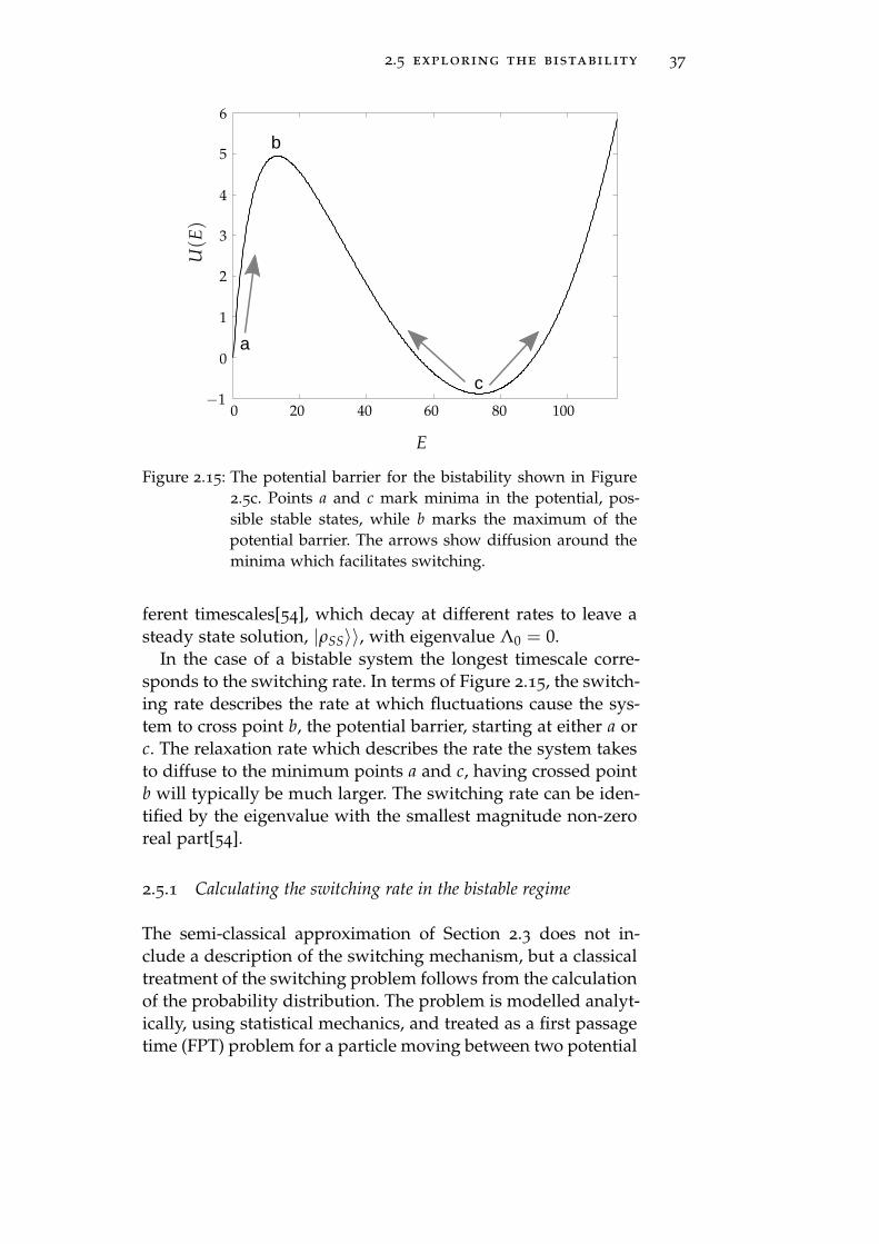
2.5 exploring the bistability 37
−1
0
1
2
3
4
5
6
0 20 8040 10060
E
U(E
)
a
b
c
Figure 2.15: The potential barrier for the bistability shown in Figure
2.5c. Points a and c mark minima in the potential, pos-
sible stable states, while b marks the maximum of the
potential barrier. The arrows show diffusion around the
minima which facilitates switching.
ferent timescales[54], which decay at different rates to leave a
steady state solution, |ρSS〉〉, with eigenvalue Λ0 = 0.
In the case of a bistable system the longest timescale corre-
sponds to the switching rate. In terms of Figure 2.15, the switch-
ing rate describes the rate at which fluctuations cause the sys-
tem to cross point b, the potential barrier, starting at either a or
c. The relaxation rate which describes the rate the system takes
to diffuse to the minimum points a and c, having crossed point
b will typically be much larger. The switching rate can be iden-
tified by the eigenvalue with the smallest magnitude non-zero
real part[54].
2.5.1 Calculating the switching rate in the bistable regime
The semi-classical approximation of Section 2.3 does not in-
clude a description of the switching mechanism, but a classical
treatment of the switching problem follows from the calculation
of the probability distribution. The problem is modelled analyt-
ically, using statistical mechanics, and treated as a first passage
time (FPT) problem for a particle moving between two potential

38 the reflective optomechanical system
wells[50]. Results are then compared to numerics which solve
the eigenvalue equation, as described below.
The analytic calculation employs a classical description of the
problem within the truncated Wigner formalism described in
Section 2.3. The objective is to calculate the average time for a
particle in one potential well to overcome the energy barrier (by
energy fluctuations) and reach the other well. This assumes the
dynamics are governed by a Fokker-Planck equation. Turning
points in the potential are found in order to calculate the FPT
for a system initially in either potential well. The switching rate
is then given by the sum of their inverses.
The calculation proceeds as follows. The points of interest in
a sample potential are shown in Figure 2.15; a is an extremum at
E = 0, treated as a well, with b the barrier and c the other well.
Starting at an energy Ea near point a, the FPT is the average
time the system takes takes to pass over the potential barrier
of energy Eb at point b. Due to the separation of timescales
for switching between and relaxation into the wells, the exact
choices of starting/finishing points are not important[50] - so
long as E f inal ≥ Emax and Estart ≈ Emin, where Emax(min) is the
maximum(minimum) in the potential.
The potential in question is defined for E > 0, so that Ea is an
extremum, and diffusion from a can only occur in one direction.
Point a is therefore identified as a reflecting barrier, since it
cannot be crossed. Conversely, point b is an absorbing barrier,
so that switching is defined as the system passing through b. To
calculate the FPT, first G(E, t) is defined - this is the probability
that the system has not overcome the potential barrier at a time
t, given that it starts at an energy E in the range Ea < E < Eb:
∫ Eb
Ea
dE′P(E′, t|E, 0) ≡ G(E, t). (2.89)
The Fokker-Planck equation given in Equation 2.71 describes
the evolution of the probability distribution P(E′, t) for t > 0,
given that the system starts at an energy E at t = 0. A calcula-
tion of the FPT requires the evolution of P(E′, t) for t < t′, given
a final condition at t = t′. This is achieved by writing a back-
ward Fokker-Planck equation for the probability distribution[50].
In contrast to the forward equation, this is defined over a range
of times prior to a ‘target’ state at time t′, where the particle
overcomes the potential barrier.
In terms of P(E′, t|E, 0) - the conditional probability of find-
ing the system with an energy E′, where 0 < E′ < Eb at a

2.5 exploring the bistability 39
time t, given the system starts at an energy E at t = 0 (where
0 < E < Eb) - the backward Fokker-Planck equation is
∂tP(E′, t|E, 0) = (γ + γBA(E)) E∂EP(E′, t|E, 0)
+1
2(Dth + DBA(E)) ∂2
EP(E′, t|E, 0), (2.90)
from which an equation for G(E, t) is deduced:
∂tG(E, t)) = (γ + γBA(E)) E∂EG(E, t)
+1
2(Dth + DBA(E)) ∂2
EG(E, t), (2.91)
The average time to reach Eb, given the starting point Ea, is
given by
〈T(Ea → Eb)〉 =∫ ∞
0dtG(Ea, t), (2.92)
which allows an equation of motion for the FPT to be deduced
from Equation 2.91, and solved for T. The average time for the
system to reach Eb as a function of starting point Ea is then
T(Ea → Eb) = 2∫ Eb2
Ea
dEeU(E)∫ E
0dE′
e−U(E′)
D(E′), (2.93)
where Eb2 is a point along the potential curve where E > Eb,
to ensure integration includes the point Eb. The FPT from Ec to
Eb(< Ec) where Eb is absorbing, is found in a similar way:
T(Ec → Eb) = 2∫ Ec
Eb1
dEeU(E)∫ ∞
EdE′
e−U(E′)
D(E′), (2.94)
where Eb1 is a point along the potential curve where E < Eb.
The diffusion constant, D(E) = Dth + DBA(E), is a function
of E, so must also be integrated in the first integral (which has
variable limits). The switching rate between potential wells, Γsw,
is then given by
Γsw = [T(Ea → Eb)]−1 + [T(Ec → Eb)]
−1 . (2.95)
2.5.1.1 Comparing switch rate with lowest eigenvalue
The eigenvalues Λn that describe the relaxation of the system
(Equation 2.88) can also be calculated numerically. Figure 2.16
shows the lowest five eigenvalues from the expansion in Equa-
tion 2.88. On a logarithmic scale, the lowest eigenvalue Λ1 is
isolated from the others. The presence of an eigenvalue much

40 the reflective optomechanical system
n = 1n = 2n = 3n = 4n = 5
−2.4 −2.2 −2 −1.8 −1.6
∆
−8
−16
−14
−10
−12ln(Λ
n)
Figure 2.16: Eigenvalues, Λn, for 1 ≤ n ≤ 5 on a log scale, shown
over the bistable range. The lowest value Λ1 is isolated
and much smaller than the others. This is thought to be
a characteristic of quantum tunnelling.
closer to zero than the others is often considered a characteristic
of quantum tunnelling[54].
The eigenvalue with the smallest non-zero real part, Λ1, is
compared to the switching rate Γsw in Figure 2.17, for the bistable
range. The analytic switching rate differs by up to an order of
magnitude from the lowest eigenvalue. The two rates are plot-
ted on a logarithmic scale.
The analytically calculated Γsw underestimates the switching
rate for the range −2.5 ≤ ∆ ≤ −1.7. In the range ∆ ≤ −1.7,
however, it the rapidly increases by several orders of magni-
tude. In contrast the eigenvalue forms a roughly symmetric
well shape over a much smaller range of values. These discrep-
ancies are not unique to this particular calculation, and have
been observed as a consistent failing in the truncated Wigner
approximation[54].
Figure 2.18a shows the rates T(a → b) and T(c → b) sepa-
rately for comparison. It is apparent that the rate from a to b
reaches a much higher value than from c to b. As ∆ is swept,
the potential evolves so that the barrier moves from the vicinity
of point a to the vicinity of point c (see Figure 2.18b). As a result
T(a → b) increases with |∆| while T(c → b) decreases. How-
ever, T(a → b) undergoes a rapid increase around |∆| > 2.4
compared to the increase in T(c→ b) at |∆| < 2.

2.5 exploring the bistability 41
∆
ln (Γsw)
ln (Λ1)
−2.4 −2.2 −1.6−1.8−2−20
−15
−10
−5
Figure 2.17: Comparison between the switching rates of the system,
deduced from a numerical calculation of the eigenvalues
(solid) and the classical FPT calculation (dashed). Results
are plotted on a log scale as there is a large difference in
the results.
T
∆−2.4 −2.2 −2 −1.8
1
2
3
4
5
6
×1013
1
2
3
0
×1011
−2.4 −2.2 −2
Increase |∆|
U(E
)
E0 4020 60 80 100 120
−5
−10
−15
0
5
10
20
15 ∆ = −1.8∆ = −2∆ = −2.2∆ = −2.4
(a) (b)
Figure 2.18: The separate switching times calculated, shown in (a)
T(a → b) (solid) and T(c → b) (dashed) show maxi-
mum values at either end of the bistable regime which
differ by an order of magnitude. Over this range the po-
tential shown in (b) evolves such that the barrier height
increases(decreases) relative to the point a(c).
The asymmetry is likely caused by the way the potential is
defined. The energy can only take on positive values, and point
a lies at the extremum E = 0. It is used as a minimum in the
calculation, but it does not satisfy U′(E) = 0, nor is the system
free to diffuse in the opposite direction when placed at E = Ea.
The system is more confined about a, and therefore more likely

42 the reflective optomechanical system
to diffuse up the slope towards b, as shown by the grey arrow
in Figure 2.15. At point c, the system is free to diffuse up the
slope in either direction. As a result the switching rate in the
direction a→ b is much larger than for c→ b.
The analytic calculation is clearly unable to describe the dy-
namics of the bistable state. The FPT calculation models the
switching mechanism classically, as fluctuation in the system’s
energy causing it to overcome the potential barrier[50]. This
does not account for the quantum tunnelling suggested by Fig-
ure 2.16. In systems where tunnelling occurs, the truncated Wig-
ner approximation is known to fail at capturing the switching
rate[1, 54]. The quantum fluctuations, which induce switching
on a much faster timescale, are only partly included because
the third order derivatives are dropped. This supports the fact
that analytics predict a much slower switching rate.
2.5.2 Relaxation rate calculation
If the switching rate is given by the lowest non-zero eigenvalue,
the next lowest should give the relaxation rate of the system
within each potential well. Once a particle has overcome the
barrier, this rate describes how long the system takes to relax
into the potential well. These rates can be calculated analyti-
cally by looking at the dynamics of the average energy (eg by
averaging Equation 2.61),
〈E〉 = −[γ + γBA(E)]〈E〉. (2.96)
Equation 2.96 is expanded in terms of small fluctuations, δE′
about the limit cycle at E0:
˙δE = − [γ + γBA(E0)] δE + E0dγBA
dE
∣
∣
∣
E0
δE, (2.97)
where second order fluctuations are discarded.
One can consider the case of a fixed point (where E0 = 0),
giving a relaxation rate Γr of
Γr(E0 = 0) = γ + γBA(0). (2.98)
For a limit cycle the first term in Equation 2.97 will vanish giv-
ing the relaxation rate,
Γr(E0 6= 0) = E0dγBA
dE|E0
. (2.99)

2.5 exploring the bistability 43
2.5.2.1 Comparing relaxation rate with eigenvalues
Figure 2.19 shows the relaxation rates given by Equations 2.98
and 2.99, plotted alongside the eigenvalues, Λn, for 1 ≤ n ≤ 3.
Far from the bistable regime, in regions |∆| ≤ 1.5 and |∆| ≥3.25, the analytic calculation closely matches the lowest non-
zero eigenvalue. In particular, the relaxation into the limit cy-
cle state is captured well. Within the bistable regime, however,
the calculation fails. Equations 2.98 and 2.99 are deduced by
ignoring second order fluctuations in the energy, under the as-
sumption that these are small. This does not hold in the bistable
regime, so expressions 2.98 and 2.99 fail here.
Γr(
E=
0)
∆
Γr (E
0 6=0)
0−5 −4 −3 −2 −1
2
6
4
8
14
10
12
×10−5
Figure 2.19: Comparison between analytic and numerical calculations
of relaxation rates in the system. Thicker black lines
show the relaxation rates Γr calculated analytically, for
the fixed point and limit cycle state. The lowest three non
zero eigenvalues Λn are also shown, the lowest of which
matches Γr closely far from the bistable range.
From the analysis of this section, it is apparent that the bistable
regime cannot be described by semi-classical analysis. The FPT
calculation fails to describe the true quantum nature of the
switching mechanism[54], whilst the simple linearized descrip-
tion of fluctuations misses the mark once the system enters
the bistable regime. Whilst the truncated Wigner function suc-
cessfully describes the steady-state properties of the resonator
discussed in Section 2.4.4 - even in the bistable state - it falls
44 the reflective optomechanical system
short of a more detailed analysis of the switching and relax-
ation rates.
2.6 conclusion
This chapter has explored the dynamics of a linearly coupled
optomechanical system, using the reflective setup. When a drive
is applied to the cavity, the resonator transitions between three
distinct states as the laser is tuned to different frequencies. These
include a state where the system fluctuates about a fixed point,
limit cycle oscillations and a bistability. The evolution of the
resonator state looks very different depending on whether the
system is in the resolved sideband regime. In the strong cou-
pling limit, non-classical states can be generated[10, 43]. In the
weak coupling limit, the system can be modelled analytically.
The truncated Wigner function approach provides a way of
calculating the dynamics of the system analytically provided
the optomechanical coupling is weak (i.e. λ ≪ 2ωm). In partic-
ular this approach describes the dynamics accurately when the
resonator is in a well defined limit cycle and the fluctuations
are small, but fails to fully capture the bistable regime where
fluctuations are large. An especially serious limitation of the
truncated Wigner function is the switching time for a resonator
in a bistable state. The quantum value of the switching time has
been found to differ by more than an order of magnitude from
that obtained using the truncated Wigner approximation.

3Q U A D R AT I C C O U P L I N G I N A D I S P E R S I V E
O P T O M E C H A N I C A L S E T U P
3.1 introduction
Chapter 2 addressed the case of a system in which optical and
mechanical modes are coupled via reflection of the light. This
produces an interaction which depends linearly on the posi-
tion of the mechanical oscillator. In this chapter, an alterna-
tive approach is considered in the form of a ‘dispersive system’
which uses the ‘membrane-in-the-middle’ geometry[25, 16]. A
mechanical element placed at the centre of an optical field par-
tially reflects radiation from both sides, so as to couple the op-
tical frequency linearly or quadratically to position, depending
on whether the element is placed at a node or anti-node of
the optical field[25]. This ability to switch between linear and
quadratic interactions, by altering only the membrane position,
is an attractive feature of such a system. It allows precision mea-
surements of both the position[62, 63] (in the linear case) and
energy[22] (in the quadratic case) of the mechanical element,
depending on the coupling chosen[17].
In Chapter 2 the non-linear dynamics of the reflective system
were analysed using a numerical approach, as well as a semi-
classical approximation. Analytics were generated using a trun-
cated Wigner approximation. In this chapter a similar toolbox
of mathematical techniques is applied to the quadratic system.
The aim is to calculate a probability distribution for the state of
the mechanical resonator, allowing its behaviour to be investi-
gated under different conditions.
Using a Wigner transformation, Langevin type equations are
found to describe the optical and mechanical modes. Solutions
to these equations lead to an expression for the damping due to
back action, which can be used to determine the presence of sta-
ble limit cycles in the resonator. In addition, the diffusion in the
system is calculated. Together with the damping this allows a
probability distribution of states of the resonator to be obtained.
The analytic results are compared with numerical calculations
and good agreement is found under certain circumstances. The
regime of strong coupling is also investigated, and a number of
45

46 quadratic coupling in the dispersive system
signatures of non-classical behaviour are found to occur in the
mechanical resonator.
This chapter is organised as follows. In Section 3.2 the ‘mem-
brane in the middle’ approach is introduced, detailing its for-
mulation in terms of a Hamiltonian and master equation. Sec-
tion 3.3 outlines a semi-classical analysis of the system via a
similar set of approximations to those used in Chapter 2. Nu-
merical calculations are described and analysed in Section 3.4.
The numerics are compared to analytics in Section 3.5. Section
3.6 draws conclusions.
3.2 membrane in the middle system
The system under consideration consists of two fixed mirrors
with a membrane placed in between, as shown schematically in
Figure 3.1a. The membrane divides the cavity into two cham-
bers. Consider a pair of modes (one in each chamber) with
almost identical frequencies, ωL and ωR. The membrane sup-
ports mechanical modes as it vibrates. The vibrations alter the
lengths of each chamber, coupling the membrane displacement
to the optical frequencies. A perfectly reflecting membrane dis-
placed by an amount q(t) would shift the two mode frequencies
as follows,
ωL(q) ≈ ω0 − λq(t), (3.1)
ωR(q) ≈ ω0 + λq(t), (3.2)
where ω0 is the cavity frequency in both chambers when the
membrane is fixed at the centre and λ is the coupling between
the optical and mechanical modes. This relates to the length
of each chamber, L, by λ = ω0/L. In fact the membrane is
partially transmitting, coupling the optical modes together into
two new harmonic modes with frequencies ω1 and ω2 respec-
tively (shown by the blue lines in Figure 3.1b). The strength
of the coupling is parametrised by g, which relates to the rate
at which photons tunnel through the membrane. This coupling
creates an anti crossing in their dispersion diagram[16] as shown
in Figure 3.1b. The dotted lines represent mode frequencies for
a perfectly reflecting membrane. When radiation is allowed to
pass through the membrane, the two modes become coupled,
illustrated by the two solid blue curves. The energy gap 2g
(which will be addressed in a later section) arises due to the
coupling.
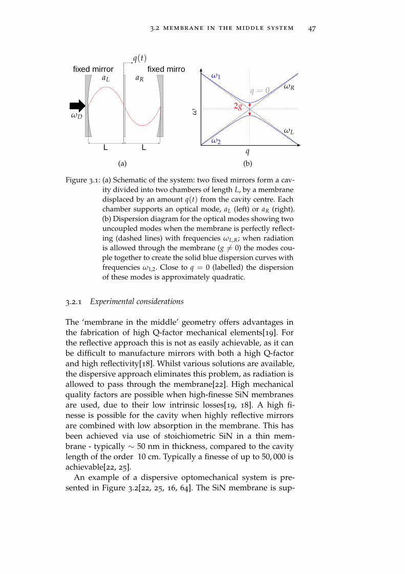
3.2 membrane in the middle system 47
L
q(t)
fixed mirror fixed mirror
L
ωD
aL aR
(a)
q
ω
ωR
ωL
ω1
ω2
2g
q = 0
(b)
Figure 3.1: (a) Schematic of the system: two fixed mirrors form a cav-
ity divided into two chambers of length L, by a membrane
displaced by an amount q(t) from the cavity centre. Each
chamber supports an optical mode, aL (left) or aR (right).
(b) Dispersion diagram for the optical modes showing two
uncoupled modes when the membrane is perfectly reflect-
ing (dashed lines) with frequencies ωL,R; when radiation
is allowed through the membrane (g 6= 0) the modes cou-
ple together to create the solid blue dispersion curves with
frequencies ω1,2. Close to q = 0 (labelled) the dispersion
of these modes is approximately quadratic.
3.2.1 Experimental considerations
The ‘membrane in the middle’ geometry offers advantages in
the fabrication of high Q-factor mechanical elements[19]. For
the reflective approach this is not as easily achievable, as it can
be difficult to manufacture mirrors with both a high Q-factor
and high reflectivity[18]. Whilst various solutions are available,
the dispersive approach eliminates this problem, as radiation is
allowed to pass through the membrane[22]. High mechanical
quality factors are possible when high-finesse SiN membranes
are used, due to their low intrinsic losses[19, 18]. A high fi-
nesse is possible for the cavity when highly reflective mirrors
are combined with low absorption in the membrane. This has
been achieved via use of stoichiometric SiN in a thin mem-
brane - typically ∼ 50 nm in thickness, compared to the cavity
length of the order 10 cm. Typically a finesse of up to 50, 000 is
achievable[22, 25].
An example of a dispersive optomechanical system is pre-
sented in Figure 3.2[22, 25, 16, 64]. The SiN membrane is sup-

48 quadratic coupling in the dispersive system
ported by a frame and positioned between two mirrors, M1
and M2, mounted on a cavity spacer, inside a vacuum cham-
ber. An Nd:YAG laser provides the drive1[65]. The beam is
passed through an optical isolator (OFR) and into the cavity,
via two steering mirrors, SM1 and SM2. The output from the
cavity is fed through a photodiode (PD) which measures the
optical power transmitted and feeds it into a digital storage os-
cilloscope. This way one can measure the optical frequency of
modes in the cavity, from which the mechanical position can be
deduced.
Figure 3.2: Schematic of a typical membrane in the middle experi-
mental setup[64]. See text of Subsection 3.2.1 for further
details.
3.2.2 The Hamiltonian and master equation
In this chapter, quadratic optomechanical coupling is explored.
This can arise for the membrane in the middle geometry, illus-
trated in Figure 3.1a. The Hamiltonian can be derived by consid-
ering the modes of the whole cavity[18, 19]. Here the quadratic
Hamiltonian is motivated using a simple model, which starts
from a description in terms of the modes of the left and right
sub-cavities (see Figure 3.1a) and allows for partial transmis-
1 neodymium-doped yttrium aluminium garnet is a crystal, widely used asa lasing medium for solid-state lasers. The neodymium ions provide a four-level system.

3.2 membrane in the middle system 49
sion. In terms of these two modes (shown as dashed lines in
Figure 3.1b) the Hamiltonian takes the form
H = ωL(q)a†LaL + ωR(q)a†
RaR + g(a†LaR + a†
RaL)
+1
2ωm(p2 + q2) + Ω(aLeiωdt + a†
Le−iωdt), (3.3)
where aL(aR) is the annihilation operator for the left(right) mode
and the left mode is assumed to be driven with strength Ω,
at frequency ωd. The membrane’s displacement is taken as q,
with momentum p, and frequency ωm. The optical frequen-
cies are functions of q, given by Equations 3.1 and 3.2. Note
that in terms of resonator raising(lowering) operators b†(b), q =(
b + b†)
/√
2 and p =(
b− b†)
/(√
2i).Since the cavity modes couple together, it can be more intu-
itive to write the Hamiltonian in terms of the upper and lower
dispersion bands (solid blue lines in Figure 3.1b), represented
by annihilation operators a1 and a2. The transformation is linear
and of the form (for details, see Appendix D):
a1 = uaL + vaR, (3.4)
a2 = xaL + yaR, (3.5)
with coefficients
u =g
√
g2 + (ω1 −ωL)2(3.6)
v =ω1 −ωL
√
g2 + (ω1 −ωL)2(3.7)
x =ω2 −ωR
√
g2 + (ω2 −ωR)2(3.8)
y =g
√
g2 + (ω2 −ωR)2, (3.9)
where ω1 and ω2 are given by
ω1 = ω0 +√
g2 + (λq)2 (3.10)
ω2 = ω0 −√
g2 + (λq)2. (3.11)
This then allows the Hamiltonian to be written in the following
form:
H = ω1a†1a1 + ω2a†
2a2 +1
2ωm(p2 + q2)
+Ω[(Xa1 −Ya2)eiωdt + (Xa†
1 −Ya†2)e−iωdt], (3.12)

50 quadratic coupling in the dispersive system
where X and Y are given by
X =g√
g2 + (ω1 −ωL)2
g2 − (ω1 −ωL)(ω2 −ωR), (3.13)
Y =(ω1 −ωL)
√
g2 + (ω2 −ωR)2
g2 − (ω1 −ωL)(ω2 −ωR). (3.14)
The coupled frequencies ω1,2 have a dependence on q which
is approximately quadratic when g≫ λq
ω1 ≈ ω0 +[
g +λ2
2gq2]
, (3.15)
ω2 ≈ ω0 −[
g +λ2
2gq2]
. (3.16)
Thus by probing the dynamics around q ≈ 0, the case of quad-
ratic optomechanical coupling is explored.
The minimum frequency gap is 2g, as shown in Figure 3.1b.
For g ≫ ωm, the upper and lower modes are separated by a
large enough frequency that there is little chance of transitions
between them. This allows a single mode to be considered by
selecting a drive frequency close to its resonance. This chapter
focuses on a single optical mode with frequency ω1, and the
corresponding annihilation operator is labelled simply a. The
effects of quadratic coupling to the mechanical resonator can
then be analysed.
In Chapter 2, Equations 2.11 to 2.15 detail a unitary transfor-
mation on the Hamiltonian. An identical transformation gives
the effective Hamiltonian for the quadratically coupled system,
in the rotating frame of the drive frequency:
He f f = ∆a†a + Gq2a†a +1
2ωm(p2 + q2) + ǫ(a + a†), (3.17)
where ∆ = ω0 + g− ωd, ǫ = ΩX, G = λ2/(2g). Note that the
implicit q dependence in the drive term that arises through X
is neglected in the following. The master equation is written in
terms of ρ, the density operator in this rotating frame:
˙ρ = −i[
He f f , ρ]
+ Laρ + Lbρ. (3.18)
The same model as that introduced in Chapter 2 is applied to
describe dissipation in the cavity and resonator in terms of two
separate environments of harmonic oscillators which couple to
each set of modes separately. This results in operators La and

3.3 semi-classical approximation 51
Lb identical to the linear case (where again it is assumed that
na = 0):
Laρ = −κ
2
(
a†aρ + ρa†a− 2a†ρa)
, (3.19)
Lbρ = −γ
2(n + 1)
(
b†bρ + ρb†b− 2b†ρb)
−γ
2n(
bb†ρ + ρbb† − 2bρb†)
. (3.20)
The analysis that follows employs a very similar combina-
tion of analytical and numerical methods to those used for the
linearly coupled system. The next section details an analytic
approach via a semi-classical approximation, before further sec-
tions discuss numerical results.
3.3 semi-classical approximation
3.3.0.1 Wigner transformation
The semi-classical approach follows an analogous procedure to
Chapter 2. Once again, the truncated Wigner approximation is
employed to obtain a Fokker-Planck equation describing the
evolution of the quasi-probability distribution for the coupled
system. Previously this proved effective in describing the lin-
early coupled system, with the only notable discrepancies be-
ing a shift in ∆[30] and a failure to predict quantum tunnelling
rates[54].
The transformation is detailed in Appendix A. Here the re-
sults are presented in a similar framework to Chapter 2. The
truncated equation is
∂W
∂t=
∂
∂β∗
(
− iωmβ∗ +γ
2β∗ − 2iG(β∗ + β)(α∗α− 1
2))
W
+∂
∂β
(
iωmβ +γ
2β + 2iG(β∗ + β)(α∗α− 1
2))
W
+∂
∂α∗
(
− i∆α∗ +κ
2α∗ − iGα∗(β∗ + β)2 − iǫ∗
)
W
+∂
∂α
(
i∆α +κ
2α + iGα(β∗ + β)2 + iǫ
)
W
+γ
2(2n + 1)
∂2W
∂β∂β∗+
κ
2
∂2W
∂α∂α∗, (3.21)
where once again the phase space variables α and β replace the
quantum operators a and b, and the shorthand W = W(α, β) is

52 quadratic coupling in the dispersive system
used for the Wigner function. Langevin equations for α, α∗, β
and β∗ follow from Equation 3.21[1]:
α = −i∆α− iGα(β + β∗)2 − κ
2α− iǫ + ηα, (3.22)
α∗ = i∆α∗ + iGα∗(β + β∗)2 − κ
2α∗ + iǫ + ηα∗ , (3.23)
β = −iωmβ− 2iG(β + β∗)(
α∗α− 1
2
)
− γ
2β + ηβ(3.24)
β∗ = iωmβ∗ + 2iG(β + β∗)(
α∗α− 1
2
)
− γ
2β∗+ηβ∗ ,(3.25)
where, as previously, ηα and ηβ are Gaussian white noise vari-
ables, describing fluctuations in variables α and β.
3.3.1 Analysis of the Langevin equations
As in Chapter 2, an analytic calculation considers the regime
where optical timescales are much faster than mechanical ones.
In particular, it is assumed that κ ≫ γ, G, so the rate at which
the energy of the mechanical resonator changes is much slower
than that of the optical mode. This allows β = Be−i(ω′mt+φ) to
be substituted into Equation 3.22, where φ is a phase variable
and ω′m = ωm + δω. The shifted mechanical frequency, ω′m, will
be determined self-consistently. Since the coupling is quadratic
with position, oscillations occur around the centre of the cavity,
so that βc = 0. With the quantities B, δω and φ treated as con-
stants (See Chapter 2, Section 2.3.1 for details), Equation 3.22 is
written
α = −[
i∆′ +κ
2+ 2iB2G cos (2(ω′mt + φ))
]
α− iǫ
+ηα, (3.26)
where ∆′ = ∆ + 2B2G. The calculation proceeds almost identi-
cally to Chapter 2. A substitution, α = αeiz sin (2(ω′mt+φ)), is made,
where z = B2G/ωm:
˙α = −[
i∆′ +κ
2
]
α− iǫ
2πeiz sin (2(ω′mt+φ)) + ηα. (3.27)
The equation is Fourier transformed, separated into average
and fluctuating parts, and the Jacobi-Anger expansion[55] ap-
plied to express α(ω) in terms of a Bessel series:
α(ω) = 〈α(ω)〉+ δα(ω), (3.28)
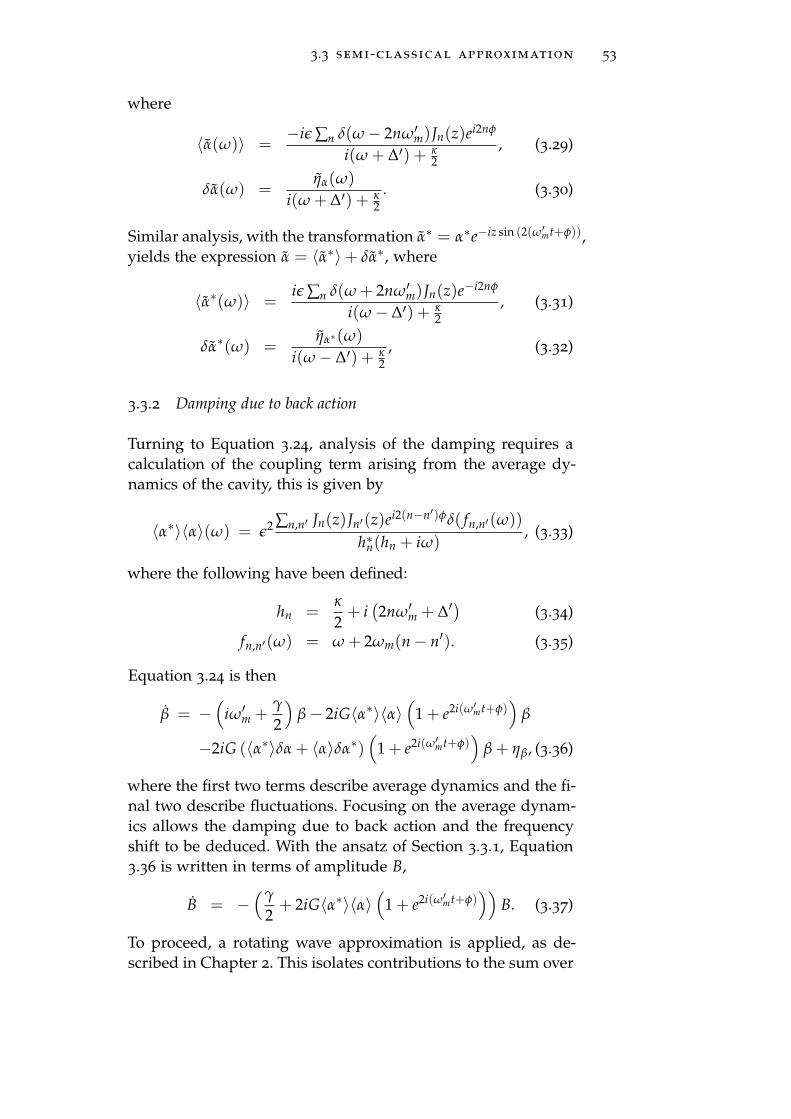
3.3 semi-classical approximation 53
where
〈α(ω)〉 =−iǫ ∑n δ(ω− 2nω′m)Jn(z)ei2nφ
i(ω + ∆′) + κ2
, (3.29)
δα(ω) =ηα(ω)
i(ω + ∆′) + κ2
. (3.30)
Similar analysis, with the transformation α∗ = α∗e−iz sin (2(ω′mt+φ)),
yields the expression α = 〈α∗〉+ δα∗, where
〈α∗(ω)〉 =iǫ ∑n δ(ω + 2nω′m)Jn(z)e−i2nφ
i(ω− ∆′) + κ2
, (3.31)
δα∗(ω) =ηα∗(ω)
i(ω− ∆′) + κ2
, (3.32)
3.3.2 Damping due to back action
Turning to Equation 3.24, analysis of the damping requires a
calculation of the coupling term arising from the average dy-
namics of the cavity, this is given by
〈α∗〉〈α〉(ω) = ǫ2 ∑n,n′ Jn(z)Jn′(z)ei2(n−n′)φδ( fn,n′(ω))
h∗n(hn + iω), (3.33)
where the following have been defined:
hn =κ
2+ i(
2nω′m + ∆′)
(3.34)
fn,n′(ω) = ω + 2ωm(n− n′). (3.35)
Equation 3.24 is then
β = −(
iω′m +γ
2
)
β− 2iG〈α∗〉〈α〉(
1 + e2i(ω′mt+φ))
β
−2iG (〈α∗〉δα + 〈α〉δα∗)(
1 + e2i(ω′mt+φ))
β + ηβ, (3.36)
where the first two terms describe average dynamics and the fi-
nal two describe fluctuations. Focusing on the average dynam-
ics allows the damping due to back action and the frequency
shift to be deduced. With the ansatz of Section 3.3.1, Equation
3.36 is written in terms of amplitude B,
B = −(γ
2+ 2iG〈α∗〉〈α〉
(
1 + e2i(ω′mt+φ)))
B. (3.37)
To proceed, a rotating wave approximation is applied, as de-
scribed in Chapter 2. This isolates contributions to the sum over

54 quadratic coupling in the dispersive system
n′ that produce terms oscillating at ω′m, whilst other terms ro-
tate rapidly and can be discarded[56]. The resulting equation
is
B = −(γ
2+ Γ
)
B, (3.38)
where
Γ = 2iGǫ2 ∑n
(
J2n(z)
|hn|2+
Jn(z)Jn+1(z)
hn+1h∗n
)
, (3.39)
and
hn =κ
2+ i(2nω′m + ∆′). (3.40)
Note that the φ dependence is lost and so the resulting damp-
ing expression will only depend on B and ω′m. The damping
and frequency shift are identified as the real and imaginary
components of the coupled term, respectively:
γBA(z) = −4Gκω′mǫ2 ∑n
Jn(z)Jn+1(z)
| hn |2| hn+1 |2, (3.41)
δω(z) = 2Gǫ2 ∑n
[
Jn(z)2
| hn |2− Jn(z)Jn+1(z)χn
| hn |2| hn+1 |2]
, (3.42)
where
χn = κ2/4 +(
2(n + 1)ω′m + ∆′)
(2nω′m + ∆′). (3.43)
In Chapter 2 the correction ω′ = ωm + δω results in negligible
errors in γBA, so it was ignored and ωm used throughout. For
the quadratic case, the errors are slightly higher (around 10−2
for the parameters considered) and the correction is added in.
The shift δω(z) is calculated using the un-shifted frequency ωm,
before using the shifted frequency ω′m to calculate γBA(z) and
δω(z).Figure 3.3 shows the damping due to back-action on a colour
plot for different energies as ∆ is varied. The white contour
shows solutions to the energy balance condition for limit cycles:
γ + γBA(E0) = 0, (3.44)
where γBA(E0) is the damping due to back action as a function
of energy, at point E0 = B20. For each value of ∆ either two
solutions occur, or there is no limit cycle. The stability condition
for a limit cycle requires γ′BA(E0) > 0, which results in stable
limit cycles at the higher energy end of the contour.

3.3 semi-classical approximation 55
80
20
40
−5 −2 −1 0 1−3−4
E
∆
6
0
4
−2
2
−4
−6
×10−3
γB
A
0
60
100
Figure 3.3: The damping due to back action, with respect to energy
E and detuning ∆. White regions signify heavy damping
whilst darker regions show strong driving. The white con-
tour marks solutions to the energy balance condition, for
limit cycles. For each value of ∆, there is either no limit cy-
cle or two solutions occur at different energies. The higher
energy solutions are found to be stable. Parameters used
are G = 0.03, ǫ = 0.4, γ = 1.4× 10⁻³ and κ = 1.
It is worth noting the behaviour of γBA at E = 0. Taking
z≪ 1, the asymptotic Bessel function behaviour is considered:
Jn(z) ≈1
n!
( z
2
)n. (3.45)
The damping is then approximated by the leading terms in the
sum, n = 0 and n = −1,
γBA ≈16Gκω2
mǫ2∆′z
[ κ2
4 + ∆′][ κ2
4 + (2ωm + ∆′)2][ κ2
4 + (2ωm − ∆′)2]. (3.46)
The back action damping is thus proportional to E as E→ 0, so
that γBA(0) = 0. This results in a total damping which is always
positive in the low energy limit, so that the stability condition
on the fixed point at the origin (E = 0), γ + γBA(0) > 0, is
always satisfied. The fixed point is therefore always a stable
solution for the case of quadratic coupling.

56 quadratic coupling in the dispersive system
3.3.3 Diffusion due to back action
With the intention of including fluctuations in the analysis, Equa-
tion 3.24 is written in terms of energy:
E = −γTE + ηT
√E, (3.47)
where γT = γ + γBA(E), and γBA(E) is given by Equation 3.41,
noting that z = GE/ωm. The fluctuating terms are given by
ηT(ω, E) =(
ηβeiωmt+φ + η∗βe−(iωmt+φ) + ηBA(ω, E))
,(3.48)
where
ηBA(ω, E) = 2√
E(
ηe f f + η∗e f f
)
sin (2ω′mt + 2φ), (3.49)
ηe f f = 2G〈α∗〉δα. (3.50)
Note that, once again second order fluctuations have been ap-
proximated by their averages, and do not contribute towards
the diffusion. Using the same approach as Chapter 2, Section
2.3.4, the diffusion is described by the expression
DBA(z) = limω′→0
ω′
2π
∫ 2π/ω′
0dt∫ ∞
−∞dωei(ωt+ω′t′)ζ(ω, ω′)(3.51)
where
ζ(ω, ω′) = 〈ηBA(ω)ηBA(ω′)〉. (3.52)
Following a similar series of steps to the linear case, the diffu-
sion constant due to back action is given by
DBA(z) = 2Gǫ2ω2mκz ∑
n
[
J2n(z)
| hn |2(
1
| hn+1 |2+
1
| hn−1 |2)
− Jn(z)Jn+2(z)
| hn+1 |2(
1
h∗nhn+2+
1
hnh∗n+2
)
]
. (3.53)
In the small energy limit, z ≪ 1, one can apply a similar ap-
proximation to that applied to the damping in Section 3.3.2.
The resulting expression for DBA then contains a contribution
from the n = 0 term only:
DBA ≈2Gκωmǫ2
(
κ2
4 + ∆′2 + 4ω2m
)
z[
κ2
4 + ∆′2] [
κ2
4 + (2ωm + ∆′)2] [
κ2
4 + (2ωm − ∆′)2] .(3.54)
It is interesting to note that both the diffusion and damping
due to back action are approximately linear at small energies,
in contrast to the linearly coupled system, where both tend to-
wards constants as E → 0. This will be important when ad-
dressing the cooling regime.
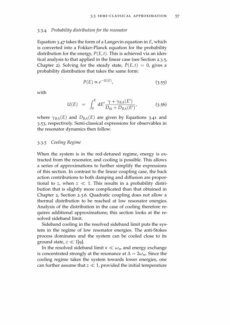
3.3 semi-classical approximation 57
3.3.4 Probability distribution for the resonator
Equation 3.47 takes the form of a Langevin equation in E, which
is converted into a Fokker-Planck equation for the probability
distribution for the energy, P(E, t). This is achieved via an iden-
tical analysis to that applied in the linear case (see Section 2.3.5,
Chapter 2). Solving for the steady state, P(E, t) = 0, gives a
probability distribution that takes the same form:
P(E) ∝ e−U(E), (3.55)
with
U(E) =∫ E
0dE′
γ + γBA(E′)Dth + DBA(E′)
, (3.56)
where γBA(E) and DBA(E) are given by Equations 3.41 and
3.53, respectively. Semi-classical expressions for observables in
the resonator dynamics then follow.
3.3.5 Cooling Regime
When the system is in the red-detuned regime, energy is ex-
tracted from the resonator, and cooling is possible. This allows
a series of approximations to further simplify the expressions
of this section. In contrast to the linear coupling case, the back
action contributions to both damping and diffusion are propor-
tional to z, when z ≪ 1. This results in a probability distri-
bution that is slightly more complicated than that obtained in
Chapter 2, Section 2.3.6. Quadratic coupling does not allow a
thermal distribution to be reached at low resonator energies.
Analysis of the distribution in the case of cooling therefore re-
quires additional approximations; this section looks at the re-
solved sideband limit.
Sideband cooling in the resolved sideband limit puts the sys-
tem in the regime of low resonator energies. The anti-Stokes
process dominates and the system can be cooled close to its
ground state, z≪ 1[9].
In the resolved sideband limit κ ≪ ωm and energy exchange
is concentrated strongly at the resonance at ∆ = 2ωm. Since the
cooling regime takes the system towards lower energies, one
can further assume that z≪ 1, provided the initial temperature

58 quadratic coupling in the dispersive system
is not too high. With these assumptions, Equations 3.46 and 3.54
gives
γBA(z) ≈2Gǫ2z
κωm(3.57)
DBA(z) ≈Gǫ2z
κωm(3.58)
A simple expression for the probability distribution can be
found when thermal fluctuations dominate, DBA/Dth ≪ 1. Equa-
tion 3.55 then approximates to
P(E) ∝ e− ǫ2G2E2
κγω2mn e−
En , (3.59)
In the limit ǫ2G2/κγω2m ≪ n the distribution behaves as a de-
caying exponential. This limit is depicted in Figure 3.4, which
shows the damping and probability distribution. Here the in-
trinsic damping dominates so the approximated probability dis-
tribution is accurate, whilst the approximation in Equation 3.57
begins to diverge for E > 1.
0 2 41 3 50
1
2
×10−4
γB
A
E0 2 41 3 5
P(E
)
E
(a) (b)
0
0.05
0.15
0.1
0.2
Figure 3.4: Analytics for ωm = 5, γ = 0.1, ǫ = 0.4, n = 5, G =
0.03. Solid lines represent the small energy approximation,
whilst dashed lines give the semi-classical approximation.
Figures show (a) damping due to back action and (b) prob-
ability distribution.
It should be noted that the results presented in this limit
match those in recent work by Nunnenkamp et al.[45]. In con-
trast to the analysis of this section, Nunnenkamp et al. derive
their expression for the probability distribution by deriving an
effective classical master equation directly from the full quan-
tum master equation.

3.4 numerical analysis 59
3.4 numerical analysis
In this section the numerical solution to the master equation
is explored, focusing especially on the blue-detuned regime
where limit cycles occur. The analysis addresses the cases of
strong and weak optomechanical coupling.
The coupling determines the strength of the non-linearity,
which affects the type of behaviour seen in the resonator[66].
Analysis deals with the weak and strong coupling limits sep-
arately. At weak coupling, G ≪ κ, the analytic calculations
are expected to capture the behaviour of the resonator. In the
strong coupling regime, G ≫ κ, the fundamental assumption
of the semi-classical approximation is expected to break down,
since the third order differentials are proportional to G. This
regime can therefore only be explored numerically. Since the
two Hamiltonians differ only by a coupling term, the quadratic
system is expected to show similar features to the linear system
as G → 0. Plots are presented which examine the average be-
haviour of the phonon number, 〈n〉, Fano factor, F and Wigner
function of the resonator.
3.4.1 Weak coupling
For the case of weak coupling, the parameters of Table 3.1 are
investigated.
Table 3.1: Table of parameters.
Parameter Value (units κ = 1)
ωm 1
κ 1
γ 1.4× 10⁻³
G 0.03
ǫ 0.4
n 0.1
In the case of a quadratic interaction, sweeping through ∆
would be expected to reveal a series of resonance peaks at in-
tervals of 2ωm in the good cavity regime. This is due to interac-
tions occurring where pairs of phonons are transferred to the
resonator, a characteristic of the quadratic interaction. Analysis
focuses on the ‘bad cavity’ limit, where the resonance peaks
are not resolved, and the energy exchange occurs over a broad
range of frequencies.
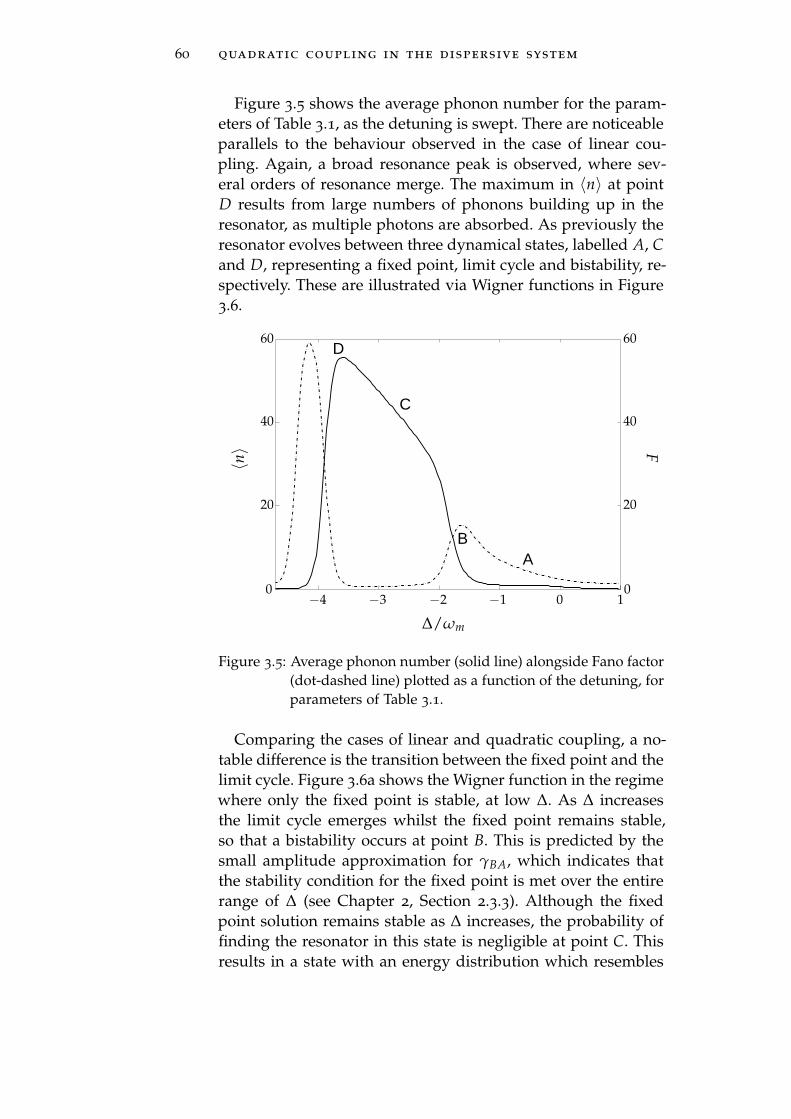
60 quadratic coupling in the dispersive system
Figure 3.5 shows the average phonon number for the param-
eters of Table 3.1, as the detuning is swept. There are noticeable
parallels to the behaviour observed in the case of linear cou-
pling. Again, a broad resonance peak is observed, where sev-
eral orders of resonance merge. The maximum in 〈n〉 at point
D results from large numbers of phonons building up in the
resonator, as multiple photons are absorbed. As previously the
resonator evolves between three dynamical states, labelled A, C
and D, representing a fixed point, limit cycle and bistability, re-
spectively. These are illustrated via Wigner functions in Figure
3.6.
0
20
40
60
0
20
40
60
−4 −2 0 1
〈n〉 F
−3 −1
AB
C
D
∆/ωm
Figure 3.5: Average phonon number (solid line) alongside Fano factor
(dot-dashed line) plotted as a function of the detuning, for
parameters of Table 3.1.
Comparing the cases of linear and quadratic coupling, a no-
table difference is the transition between the fixed point and the
limit cycle. Figure 3.6a shows the Wigner function in the regime
where only the fixed point is stable, at low ∆. As ∆ increases
the limit cycle emerges whilst the fixed point remains stable,
so that a bistability occurs at point B. This is predicted by the
small amplitude approximation for γBA, which indicates that
the stability condition for the fixed point is met over the entire
range of ∆ (see Chapter 2, Section 2.3.3). Although the fixed
point solution remains stable as ∆ increases, the probability of
finding the resonator in this state is negligible at point C. This
results in a state with an energy distribution which resembles
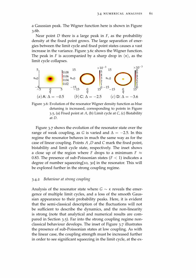
3.4 numerical analysis 61
a Gaussian peak. The Wigner function here is shown in Figure
3.6b.
Near point D there is a large peak in F, as the probability
density at the fixed point grows. The large separation of ener-
gies between the limit cycle and fixed point states causes a vast
increase in the variance. Figure 3.6c shows the Wigner function.
The peak in F is accompanied by a sharp drop in 〈n〉, as the
limit cycle collapses.
0.020.040.060.08
12345
0
×10−3
−5 50q
p
−5
5
0
12345
0
6
−15 150−15
15
0
−15 150−15
15
0
×10−3
p
q q
p
(a)A: ∆ = −0.5 (b) (c)C: ∆ = −2.5 D: ∆ = −3.6
Figure 3.6: Evolution of the resonator Wigner density function as blue
detuning is increased, corresponding to points in Figure
3.5, (a) Fixed point at A, (b) Limit cycle at C, (c) Bistability
at D.
Figure 3.7 shows the evolution of the resonator state over the
range of weak coupling, as G is varied and ∆ = −2.5. In this
regime the resonator behaves in much the same way as for the
case of linear coupling. Points A ,D and C mark the fixed point,
bistability and limit cycle state, respectively. The inset shows
a close up of the region where F drops to a minimum F ≈0.83. The presence of sub-Poissonian states (F < 1) indicates a
degree of number squeezing[10, 30] in the resonator. This will
be explored further in the strong coupling regime.
3.4.2 Behaviour at strong coupling
Analysis of the resonator state where G ∼ κ reveals the emer-
gence of multiple limit cycles, and a loss of the smooth Gaus-
sian appearance to their probability peaks. Here, it is evident
that the semi-classical description of the fluctuations will not
be sufficient to describe the dynamics, and the non-linearity
is strong (note that analytical and numerical results are com-
pared in Section 3.5). Far into the strong coupling regime non-
classical behaviour develops. The inset of Figure 3.7 illustrates
the presence of sub-Poissonian states at low coupling. As with
the linear case, the coupling strength must be increased further
in order to see significant squeezing in the limit cycle, at the ex-

62 quadratic coupling in the dispersive system
F = 1
0
20
40
60
0
20
40
60
0.040.030.020.01
G
〈n〉 F
0.20.1 0.3
1
0.6
0.8
1.2
1.4
A
C
D
Figure 3.7: Average phonon number (solid) and Fano Factor (dot-
dash) with respect to the mechanical coupling, G. The in-
set shows where the Fano factor passes below unity.
pense of encountering dynamical multistability, which causes
F ≥ 1. The dynamics in this regime are reminiscent of the lin-
ear coupling case, but some key differences are highlighted in
the analysis to follow. As the coupling is increased negative
regions occur in the Wigner function. These are explored sepa-
rately below. The parameters used are the same as in Table 3.1,
except n = 0, whilst G is varied.
3.4.2.1 Negative regions in the Wigner function
Whilst Figure 3.7 displays the presence of sub-Poissonian states,
non-classical features are stronger when n = 0[12]. Figure 3.8
shows the Fano factor over a broad range of coupling values,
with n = 0. At G = 0.04 (labelled X) the Fano factor drops to a
minimum F ≈ 0.6. The corresponding probability distribution
at this point is shown in the inset (red). These states are num-
ber squeezed[10, 12]. As the coupling is increased, the peak
grows narrower as seen at point Y (green). With increasing cou-
pling the peak grows narrower, but an additional peak emerges
(shown by the blue distribution at point Y). This causes the
Fano factor to increase, rising above above unity as the separa-
tion between the peaks increases.
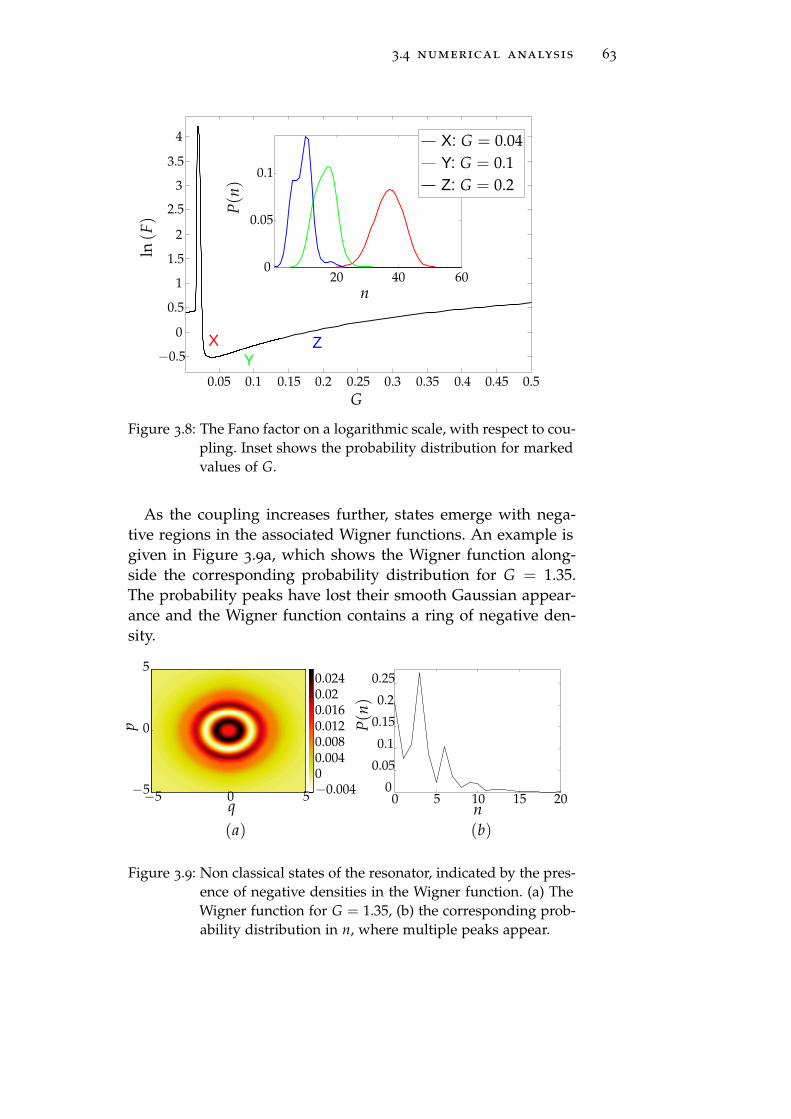
3.4 numerical analysis 63
ln(F
)
G
P(n)
n20 40 60
0
0.05
0.1
0.150.05 0.25 0.35 0.450.1 0.2 0.3 0.4 0.5
−0.5
0.5
1.5
2.5
3.5
0
1
2
3
4
XY
Z
X: G = 0.04
Y: G = 0.1
Z: G = 0.2
Figure 3.8: The Fano factor on a logarithmic scale, with respect to cou-
pling. Inset shows the probability distribution for marked
values of G.
As the coupling increases further, states emerge with nega-
tive regions in the associated Wigner functions. An example is
given in Figure 3.9a, which shows the Wigner function along-
side the corresponding probability distribution for G = 1.35.
The probability peaks have lost their smooth Gaussian appear-
ance and the Wigner function contains a ring of negative den-
sity.
q
p
0.020.0160.0120.0080.0040
0.024
−0.004−5 50−5
0
5
(a)
0 5 10 15 20
P(n)
n
0
0.1
0.2
0.05
0.15
0.25
(b)
Figure 3.9: Non classical states of the resonator, indicated by the pres-
ence of negative densities in the Wigner function. (a) The
Wigner function for G = 1.35, (b) the corresponding prob-
ability distribution in n, where multiple peaks appear.

64 quadratic coupling in the dispersive system
For states in the strong coupling regime, the extent of neg-
ativity in the Wigner functions can be measured by the ‘non-
classical ratio’[12], η. This is defined as the ratio between the
sums of the negative and positive elements in the Wigner func-
tion:
η =∑i,j |W(−)
ij |
∑k,l W(+)kl
, (3.60)
where W(+) and W(−) are the amplitudes of positive and neg-
ative Wigner elements, respectively. The sums are over all ele-
ments in the Wigner density matrix, labelled by indices i, j and
k, l.
Figure 3.10 shows numerical results in the strong coupling re-
gime, as G and ∆ are varied. The non-classical ratio is shown in
Figure 3.10a, and displays a series of peaks. Looking at lines of
constant coupling, at G < 1, the non-classical behaviour is con-
centrated towards higher order sidebands. As G is increased,
the peaks in η shift towards lower |∆|, so that for G = 3, non-
classical states are generated well below where two phonon res-
onance would be expected. It has been established in Chapter
2 that the effective value of ∆ is shifted at strong coupling for
the linear system, it seems likely that something similar is oc-
curring here.
Over the strong coupling range, F remains above unity (Fig-
ure 3.10b), whilst highly non-classical states occur. This is due
to the emergence of additional limit cycles at stronger cou-
plings. As extra peaks in P(n) emerge, F increases. As the peaks
move inwards and merge with each other, this causes drops in
F.
For highly non-classical states, the Wigner function is a se-
ries of concentric rings of densities alternating in sign, reminis-
cent of a Fock state (shown in Figure 2.11 of Chapter 2). The
corresponding probability distribution consists of a number of
sharp peaks, the separation of which results in an overall super-
Poissonian state, F > 1, whilst displaying non-classicality[12].
This behaviour has been examined extensively for the case of
linear coupling[10, 12], and is summarised in Chapter 2, Section
2.4.3.

3.4 numerical analysis 65
−5 −4 −3 −2 −1 0 10
0.01
0.02
0.03
0.04
0.05
0.06
η
∆
G
0.5
1.5
2.5
1
2
3
(a)
−5 −4 −3 −2 −1 0 1
∆
G
2
1
3
1.5
0.5
2.5
0
0.5
1
1.5
2
2.5
3
4
3.5
F
(b)
Figure 3.10: System dynamics in the strong coupling regime, as G
and ∆ are swept. (a) Non-classical ratio, as defined in
Equation 3.60, and (b) Fano factor, with ǫ = 0.4, ωm = 1,
n = 0, γ = 0.0014. In (b) the white contour indicates
the region where F < 1 - generally the strong coupling
regime produces state with F > 1, in spite of the high
non-classical ratios.

66 quadratic coupling in the dispersive system
3.5 comparison between analytics and numerics
The regime of weak coupling allows for a comparison between
analytic and numerical calculations. For the parameters of Ta-
ble 3.1, 〈n〉 and F are compared in Figures 3.11a and 3.11b for
n = 0.1, n = 1, and n = 5. Increasing the thermal phonon
number results in a broadening of the curves in 〈n〉 and F. The
off-resonance value of 〈n〉 increases and larger fluctuations al-
low phonons to build up over a wider range of ∆.
An increase in n results in greater thermal diffusion. Since
the diffusion due to back action is independent of the thermal
phonon number, at n = 5, one approaches a regime where ther-
mal fluctuations dominate2. Increasing n improves the accuracy
of the analytic solution. Figure 3.11a shows some significant dis-
crepancies, particularly at n = 0.1. These include a frequency
shift and an underestimate in the peak value of 〈n〉. As n in-
creases the shift reduces, as does the discrepancy in the peak
height. This suggests that inaccuracies in the semi-classical ap-
proximation arise largely from inaccuracies when calculating
the diffusion due to back action, which plays a more prominent
role in the dynamics as n→ 0.
The ∆ shift observed reduces as the thermal phonon number
increases, but is also found to increase with G, indicating that it
is a result of the approximate treatment of the non-linearity. In
the thermal regime, the behaviour is dominated by thermal fluc-
tuations which are described well by the semi-classical approxi-
mation. As the coupling is increased however, non-linear effects
become more prominent, and the fluctuations not treated ex-
actly by the truncated Wigner approximation cause a problem.
Figure 3.12 compares the limit cycle amplitudes deduced from
numerical and analytic calculations. The solid line represents
limit cycle energies found analytically by applying the energy
balance condition. The crosses represent the position of numer-
ical peaks in n. The data matches reasonably well, particularly
over the region where the system strongly favours the limit
cycle state, and Gaussian peaks are observed in P(n). Discrep-
ancies appear when the fixed point amplitude becomes much
larger in comparison to the limit cycle amplitude.
Overall the analytic approximation provides an accurate pic-
ture of the limit cycle dynamics, suggesting again that the an-
alytics of Figures 3.11a are limited by inaccuracies in the dif-
2 Over the range of energies considered, for parameters of case [i], DBA(E0)is of the order 10−2, compared to Dth ≈ 2.5.

3.5 comparison of results 67
〈n〉
∆/ωm
−8 −6 −4 −2 0 20
10
20
30
40
50
60
70
n = 0.1 numericaln = 0.1 analytic
n = 1 numericaln = 1 analytic
n = 5 numericaln = 5 analytic
(a)
F
∆/ωm
−8 −6 −4 −2 00
10
20
30
40
50
60
−3.5 −3 −2.5 −20.5
1
1.5
(b)
Figure 3.11: A comparison of (a) average phonon number and (b)
Fano factor, for n = 0.1 (red), n = 1 (green) and n = 5
(blue). Analytics are given by dashed lines and numer-
ics in solid, remaining parameters are as in case [i]. Inset
shows the minimum in the Fano factor for n = 0.1, where
sub-Poissonian statistics occur.
fusion calculation. Outside of the regions where the system
favours the limit cycle state, large discrepancies are found in

68 quadratic coupling in the dispersive system
〈n〉 and F. The bistable state is marked by large fluctuations
(peaks in F), resulting in greater inaccuracies in the calcula-
tion. It is apparent that the semi-classical approximation has
difficulty capturing the large fluctuations of the quadratically
coupled system.
E0
n0
−6 −4−5 −3 −2 −1
∆
10
20
30
40
50
60
70
80
90
Figure 3.12: A comparison of the limit cycle dynamics for the param-
eters of the red curve in Figure 3.11a. Analytics (solid
line) are generated via the energy balance and stability
conditions, whilst numerical points (crosses) are peaks
in P(n).
For each value of n, the agreement of the results depends
on the state of the resonator. The analytics and numerics over-
lap quite closely in the region where the system favours a sin-
gle limit cycle state. In this region, where higher energy states
are occupied, the probability distributions can be usefully com-
pared. This comparison is provided for each value of n, in
Figure 3.13. The analytic distribution P(E) (blue) is plotted
alongside numerical distribution P(n) (black). The distribution
is roughly Gaussian (the Gaussian approximation is shown in
red) and fluctuations in this region are small. The increased ac-
curacy of the semi-classical approximation is evident for n = 5.
Figure 3.14 provides a comparison between the two calcula-
tions as G is varied. At low G (see inset), the fixed point is stable
and low energies result in higher accuracy for the calculation.
As G increases, and the bistability emerges, the curves begin to

3.5 comparison of results 69
P(n),
P(E
)
n,E0 20 40 8060
0
0.02
0.04
0.06
0.08
n,E
P(n),
P(E
)
0
0.02
0.04
0.06
0.08
0 20 40 8060n,E
P(n),
P(E
)
0
0.02
0.04
0.06
0 20 40 8060 100
(a) (b) (c)∆ = −2.5 ∆ = −2.5 ∆ = −3.5
Figure 3.13: Probability distributions for the resonator in the limit cy-
cle state for (a) n = 0.1, (b) n = 1 and (c) n = 5, with
numerics in black and analytics in blue. The Gaussian
approximation is also shown in red.
diverge slightly. Larger discrepancies occur at the peak in 〈n〉.The large energies are accompanied by large fluctuations (the
inset depicts this via a sharp peak in F). These fluctuations are
not captured exactly and the analytics underestimate the peak.
Once the resonator settles into a limit cycle at high G, the fluc-
tuations reduce and the accuracy improves. The curves remain
in agreement until G ≈ 0.3, where they begin to diverge. Over-
all, the discrepancies in the curve are more pronounced as G
increases, but are also dependent on the state of the resonator.
The bistable state is generally the least accurately described by
the semi-classical approximation. In contrast, the limit cycle is
generally well described for G ≤ 0.3.

70 quadratic coupling in the dispersive system
0
5
10
15
20
25
30
35
40
45
50
〈n〉
〈n〉
G
0 0.05 0.15 0.25 0.35 0.450.1 0.2 0.3 0.4 0.5
0.050.040.01 0.02 0.03∆/ωm
F
20
40
20
40
Figure 3.14: The average phonon number with respect to G, for ∆ =
−2.5, for numerical (solid) and analytic (dashed) calcu-
lations. Inset shows 〈n〉 and F in the region of low G,
where the calculation is approximately accurate.
3.6 conclusion
This chapter has investigated an optomechanical system with
rather different geometry compared to the previous chapter. By
placing a mechanical element at the centre of a cavity and al-
lowing partial transmission of radiation, quadratic coupling is
achieved. In the blue detuned limit this system offers a range
of dynamical behaviours, similar in many aspects to the linear
case. One can observe transition between the same three res-
onator states: fixed point, limit cycle and bistability. However,
differences are observed in the transitions. The resonator passes
through two bistable regimes as the laser is tuned around the
mechanical resonance, resulting in a more symmetric looking
resonance peak in the phonon number.
The strong coupling regime offers some interesting behaviour.
As in the linearly coupled system, negative regions are observed
in the Wigner function for values of G close to unity. In addi-
tion, there are regions where number squeezing occurs (F < 1)
but these occur at much weaker couplings. It is worth noting
that, for the quadratic case, a lower value of F = 0.6 is reached,
outside of the resolved sideband limit.

3.6 conclusion 71
As in Chapter 2, the truncated Wigner approximation has
been applied to the quadratic system. The result is a similar set
of Langevin equations for the cavity and resonator. These have
been solved by separating the timescales of the cavity and res-
onator, in order to obtain a probability distribution for the res-
onator. Unfortunately the third order derivatives, which were
ignored in the approximation, turn out to have more signifi-
cance in the quadratic system. The non-linearities are stronger,
so that approximations which are valid for linear coupling lead
to inaccuracies in calculating diffusion in the quadratic case,
particularly when large fluctuations dominate the dynamics.
This results in difficulty describing the bistable regime, and the
weighting of peaks in the probability distribution are not accu-
rately captured, which results in inaccuracies in 〈n〉. However, a
certain amount of success is found in describing regions where
fluctuations are small - for example limit cycles with Gaussian
peaks. Additionally regimes such as cooling and large thermal
fluctuations are described accurately.

4S TA B I L I T Y, D A M P I N G A N D C O O L I N G I N A
T W O - M O D E S Y S T E M
4.1 introduction
The previous chapter introduced the dispersive optomechanical
system, where a membrane at the centre of the cavity provides
the mechanical mode. The coupling between the resonator and
cavity was found to range between approximately quadratic
[45] and approximately linear[67], depending on the position
of the mechanical element[17, 25]. Increasing the rate at which
photons tunnelled through the membrane increased the separa-
tion between the frequencies of the two optical modes[16], pro-
hibiting transitions and allowing a single mode to be probed
with careful selection of the drive frequency.
In this chapter the focus is shifted towards a regime where
energy exchange occurs between photonic modes as well as
with the mechanical mode. A reduced tunnelling rate through
the membrane brings the system into a regime where the fre-
quency separation between optical modes is similar to the me-
chanical frequency. In this case, the absorption or emission of
a phonon in the resonator induces transitions between photon
modes[16, 68]. As a result, one must now account for energy ex-
change between different photon modes as well as between the
cavity and resonator. The system is thus formulated in terms of
the mechanical mode and photonic modes for the left and right
chambers of the cavity.
This chapter explores the effect of damping and cooling, when
ωm ∼ g. The case of linear coupling to a single optical mode
was addressed briefly in Chapter 2, where an approximate ana-
lytical expression was obtained for the effective temperature in
the regime of sideband cooling. It has been shown theoretically
[13, 35] and experimentally[14] that a resonator can be cooled
to the quantum ground state, by coupling it to a single optical
mode.
This chapter investigates whether ground state cooling is pos-
sible for the dispersive system, in the regime where both optical
modes interact with the membrane. Since radiation is allowed
to tunnel through the mechanical element, realisation of such
73

74 cooling in a two-mode system
systems is possible without the problem of fabricating highly
reflecting mirrors with large mechanical quality factors [18, 19].
Such a feat is desirable, as it would lend itself to less challeng-
ing experimental systems.
The chapter is organised as follows: The system is introduced
in Section 4.2, and the equations of motion presented. Section
4.3 explores the static bistability, a phenomenon which arises
in strongly driven systems[69]. This allows one to determine
the regime in which the resonator reaches a stable state, a pre-
requisite for cooling. Section 4.4 explores the fluctuations and
presents a linearized calculation of the mechanical noise spec-
trum. Section 4.4.1 uses the noise spectrum to determine the
damping due to back action in the red detuned regime. This al-
lows a comparison between the single mode and double mode
systems by varying the tunnelling through the membrane. The
linearized calculation then allows an effective phonon number
to be deduced in Section 4.4.2, which also explores back action
induced cooling and compares results to the single mode case.
4.2 the system
The system under consideration takes the same basic form as
that introduced in Chapter 3 (and illustrated schematically in
Figure 3.1a), but here a rather different set of parameters are
explored. The membrane is mounted at a position q0, and has
a tunnelling rate g. In contrast to the previous Chapter, here a
regime is explored where g ∼ ωm, so that radiation is partially
reflected and partially transmitted through the membrane. The
dispersion diagram in Figure 4.1 illustrates the optical modes
in the system. For the case ωm > 2g (as is the case in Figure 4.1),
the minimum mode spacing is small enough that there exists a
displacement q′ such that the upper and lower dispersion bands
are separated by a factor of the mechanical frequency. Transi-
tions between the optical modes then occur with the absorp-
tion or emission of a phonon[16], when the system is driven
near one of the cavity frequencies.
Equation 3.3 of Chapter 3 introduces the Hamiltonian for the
dispersive system. The effective Hamiltonian is obtained, this
time, via a unitary transformation U = eiH0t with
H0 = ωd
(
a†LaL + a†
RaR
)
, (4.1)

4.2 the system 75
q
ωca
v
ωR
ωL
ωmq′
ω1
ω2
2g
Figure 4.1: Dispersion diagram showing how the frequencies optical
modes in the cavity vary with membrane displacement,
q. Uncoupled modes of frequency ωL and ωR are illus-
trated by black dashed lines, whilst the coupled modes,
ω1 and ω2, are shown in blue solid lines. The dotted grey
line marks the cavity frequency when the membrane is
at q = 0. For this example ωm > 2g and there exists a
displacement q′ for which the upper and lower dispersion
bands are separated by the mechanical frequency - this
is illustrated by the sideband (dashed curve), which are
displaced by ωm from the curves.
giving
He f f = ∆(a†LaL + a†
RaR) + g(a†LaR + a†
RaL) + λq(a†RaR − a†
LaL)
+1
2ωm(p2 + q2) + Ω(aL + a†
L), (4.2)
where the laser is detuned by ∆ = ω0 −ωd, and λ is a constant
parametrising the coupling strength.
Equations of motion can be deduced for the resonator vari-
ables q and p, as well as the cavity operators, using the input-
output formalism for optical cavities[1]. This approach takes
into account the fact that the left and right cavities are weakly
coupled to the large number of electromagnetic modes outside
the fixed mirrors[1]. The Heisenberg equations of motion of the
closed system are modified to include damping terms and fluc-
tuations described by the operators ζ (for the resonator), aINL

76 cooling in a two-mode system
(for the left cavity) and aINR (for the right cavity). The Heisen-
berg equations deduced take the form
aL = −i∆aL + iλqaL − igaR − iΩ− κ
2aL +
√κaIN
L (4.3)
aR = −i∆aR − iλqaR − igaR −κ
2aR +
√κaIN
R (4.4)
q = ωm p + ζ (4.5)
p = −ωmq− γp + λ(a†LaL − a†
RaR). (4.6)
Here the mechanical mode is subject to a viscous force, result-
ing in a damping rate γ and a Brownian stochastic force ζ[35].
This force has 〈ζ(t)〉 = 0 and is described by the correlator
〈ζ(t)ζ(t′)〉 =γ
ωm
∫
dω
2πe−iω(t−t′)ω
[
coth
(
ω
2kBT
)
+ 1
]
,(4.7)
at temperature T. The cavity, meanwhile is damped at rate κ
and subject to vacuum radiation input noise, described by the
following correlators:
〈aINL (t)aIN†
L (t′)〉 = δ(t− t′) (4.8)
〈aINR (t)aIN†
R (t′)〉 = δ(t− t′) (4.9)
where it is assumed that ωL ≫ kBT, so thermal fluctuations can
be neglected. With the intention of investigating cooling in the
two mode system, Equations 4.3 to 4.6 are expressed in terms
of small fluctuations about the mean field values: v = 〈v〉 +δv, where v = q, p, aL, aR. Separating fluctuating and average
dynamics, one then has two sets of equations to deal with:
P =γ
ωmQ (4.10)
Q =λ
ωm(|αL| − |αR|) (4.11)
αL =−iΩ
[
κ2 + i(∆R + λQ)
]
[
κ2 + i(∆R + λQ)
] [
κ2 + i(∆L − λQ)
]
+ g2(4.12)
αR =−gΩ
[
κ2 + i(∆R + λQ)
] [
κ2 + i(∆L − λQ)
]
+ g2, (4.13)
for the mean fields Q = 〈q〉, P = 〈p〉, αL = 〈aL〉 and αR = 〈aR〉.In Equations 4.12 and 4.13, the cavity equilibrium detunings ∆L
and ∆R have been introduced:
∆L = ∆− ∆ω (4.14)
∆R = ∆ + ∆ω, (4.15)

4.3 static bistability 77
with ∆ω = λq0, which parametrises the detuning between the
two cavity modes when the resonator is in the equilibrium po-
sition, q0.
The fluctuations are found to obey
δq = ωmδp (4.16)
˙δp = −ωmδq− γδp + ζ
λ(αLδa†L + α∗LδaL − αRδa†
R − α∗RδaR), (4.17)
˙δaL = −[
i∆′L +κ
2
]
δaL + iλαLδq− igδaR +√
κaINL (4.18)
˙δaR = −[
i∆′R +κ
2
]
δaR − iλαRδq− igδaL+√
κaINR , (4.19)
These equations have been linearized, so that squared fluctua-
tion terms are discarded. This requires fluctuations to be small
compared to mean field values associated with the cavity (αL
and αR) which is an appropriate assumption to make when ex-
ploring the regime of cooling. The coupling λ should also be
small. An additional frequency shift arises from the fixed point
Q, so ∆′L and ∆′R are defined:
∆′L = ∆L − λQ (4.20)
∆′R = ∆R + λQ. (4.21)
The next section deals with the fixed point analysis, before fluc-
tuations are addressed in Section 4.4.
4.3 fixed point analysis and the static bistability
This section investigates stable equilibrium positions of the res-
onator, and addresses the phenomenon of the static bistability.
This occurs when multiple fixed point solutions emerge, so that
the resonator can reach a stable state where it fluctuates about
one of two different positions. Recent publications[35, 69] have
addressed this issue, and its impact on cooling for the case of
a single optical mode. This is now extended to the two mode
case.
One can gain useful insight by considering a potential func-
tion for the mechanical resonator, deduced from the Hamilto-
nian [49]. This analysis does not account for dissipation[47, 48]
and so will not serve only as a rough guide to the fixed point
dynamics, but provides an intuitive picture of how bistability
arises. More detailed analysis follows, accounting for dissipa-
tion in the cavity and resonator modes.

78 cooling in a two-mode system
Assuming that the ring down time for the cavity modes is
short compared to the mechanical period κ > ωm, one can
adopt a simple effective potential description1. This effective po-
tential, V(q), contains a harmonic contribution, Vh = 12 ωmQ2, as
well as a contribution from the radiation pressure force acting
on the membrane, Vrad. The radiation pressure arises when the
cavity is driven, causing photons to build up in each chamber.
Collisions with the membrane exert a net force, proportional to
the difference in occupation between the left and right modes:
Frad = λ(|αL|2 − |αR|2). (4.22)
The assumption that κ > ωm allows one to calculate αL and αR
from Equations 4.12 and 4.13, assuming a fixed Q value. The
force Frad can be written as the derivative of a potential, Vrad:
Frad = −∂Vrad
∂Q(4.23)
The potential for the mechanical mode is the sum of contribu-
tions from Vrad and the harmonic restoring force,
V(Q) = Vrad +1
2ωmQ2 (4.24)
Examples of the effective potential are shown in Figure 4.2.
The red and blue curves are single well potentials, signifying
a single stability in the fixed point dynamics. As the drive
strength passes through Ω = 35.35 (green curve) a double
well emerges, indicating the presence of a static bistability. This
phenomenon has been investigated in the case of a resonator
coupled to a single cavity mode[69, 35]. As a rough estimate,
bistabilities appear where the correction to the mechanical fre-
quency is negative and of the same order as the mechanical
frequency, δω ∼ −ωm[49]. For this to occur, both cavity modes
must be red detuned (∆L, ∆R > 0) and the drive strength must
be large (Ω≫ κ).
A more general (and more formal) approach is to analyse
the stability of the fixed points in the system. The fixed points
are found by solving Equations 4.10 to 4.13 simultaneously. The
result is a fifth order polynomial in Q,
a5Q5 + a4Q4 + a3Q3 + a2Q2 + a1Q + a0 = 0, (4.25)
1 This means the cavity can be assumed to react instantaneously to the res-onator’s motion. This may not always be the case, but a more detailed anal-ysis in Section 4.3.1 accounts for κ . ωm.

4.3 static bistability 79
0
20 40 60 80 100 120
-250
-200
-150
-100
-50
Q
V
Ω = 34Ω = 35Ω = 35.35
V2
V3
V1
Figure 4.2: The mechanical potential, V(Q) = Vrad +12 ωmQ2, shown
for three different drive strengths: Ω = 34 (red), Ω = 35
(green) and Ω = 35.35 (blue). Stabilities (minima in the
curve) are marked by circles, with a bistability occurring
for Ω = 35. Parameters are ωm = 0.5, κ = 1, γ = 1× 10⁻⁴,
g = 0.1, λ = 0.01, ∆ω = 0 and ∆ = 2ωm.
with coefficients
a5 = λ4 (4.26)
a4 = 4∆ωλ3 (4.27)
a3 =
[
2
(
κ2
4− ∆R∆L + g2
)
+ 4∆ω2
]
λ2 (4.28)
a2 = 4λ∆ω
(
κ2
4− ∆R∆L + g2
)
− Ω2λ3
ωm(4.29)
a1 =
(
κ2
4− ∆R∆L + g2
)2
+ κ2∆2 − 2Ω2λ2∆R
ωm(4.30)
a0 = − λ
ωmΩ2
(
κ2
4+ ∆2
R − g2
)
, (4.31)
The polynomial in Equation 4.25 yields five possible solu-
tions for Q, not all of which are real. Since complex solutions
always appear in conjugate pairs, one finds that only one, three
or five real solutions can be found. The potential Vrad is pro-
portional to the difference in photon numbers in each chamber.
Since this is proportional to Ω2, the driving strength can be
varied to explore the emergence of bistabilities.
Figure 4.3a maps the presence of real solutions to Equation
4.25 as a function of Ω for the parameters of Figure 4.2. Over
this range of driving strengths, three solutions emerge, corre-

80 cooling in a two-mode system
sponding to the three branches of the curve. These are identi-
fied as extrema in the potential. Coloured vertical dotted lines
identify the specific parameters which produce the potentials
in Figure 4.2. Note the presence of three solutions for Ω2 = 35.
The central branch of the curve (dotted line) represents the un-
stable solution, or the maximum in the potential. The stable
branches coincide with minima in V(q).
Ω
Q
Ω0Ω1 Ω2 Ω3
33 34 35 3620
40
60
80
100
Ω
δω/
ωm
(a) (b)
0
−0.15
−0.05
−0.25
−0.1
−0.2
20 300 10
Figure 4.3: Illustration of the static bistability shown through (a) real
solutions to Equation 4.25 and (b) the resonator frequency
shift, δω (calculated later in Section 4.4.1). Stable branches
of the curves are in solid and unstable branches are dot-
ted. In (a) the three coloured vertical lines correspond
to the potentials shown in Figure 4.2, where intersec-
tions with the stable(unstable) branches correspond to
minima(maxima) in the potential. The black vertical line
is drawn at Ω0, where the instability occurs. In (b) the
coloured lines mark the region of bistability. Parameters
are the same as for Figure 4.2.
33 34 35 36
0.8
0.6
0.4
0.2
0
∆L
Ω
Figure 4.4: The detuning of the left cavity mode, as the drive strength
(as thus the fixed point displacement) is varied, causing a
cavity shift. At a point close to Ω0, the detuning becomes
negative, so that the left mode is driven above resonance.

4.3 static bistability 81
Figure 4.3a shows the presence of fixed point solutions up to
Ω = Ω0. At this point, the fixed points all become unstable and
the mechanical mode settles into a state of stable oscillations[69,
39]. Equation 4.20 describes how the red detuning in the left
cavity reduces as the fixed point position Q increases. At the
point where λQ = ∆L (marked by the horizontal dashed line),
∆′L changes sign, such that the left optical mode is driven above
resonance, and energy is no longer extracted from the resonator
to drive the cavity. It is close to this point that the instability
occurs (at Ω0) and the resonator settles into a state of fixed
amplitude oscillations. Figure 4.4 shows the detuning of the
left cavity, ∆′L, as Ω is varied, with the onset of instability Ω0
marked by a vertical black line. The three Ω values that produce
the potentials in Figure 4.2 are also shown.
Figure 4.3b indicates the behaviour of the frequency shift
over the range of Figure 4.3a. Towards the bistable region, the
frequency shift drops to a minimum, satisfying the condition
δω ∼ −ωm. Far from the bistable range, |δω| ≪ ωm, providing
a rough estimate of where static bistabilities are likely to occur.
4.3.1 Routh Hurwitz analysis
Up to this point, solving Equation 4.25 has indicated possible
fixed point solutions, with no explicit indication of their stabil-
ity. Plotting the potential at a given Ω value (Figure 4.2) indi-
cates which of the solutions occurring at that point are stable, in
the limit where κ > ωm and losses are small. A more accurate
form of stability analysis is possible by applying the Routh Hur-
witz criterion to the solutions of Equations 4.3 to 4.6. This will
provide a method of analysis which accounts for the dissipa-
tion in optomechanical systems. This criterion takes the form
of two conditions which, if met, determine that a fixed point
solution is stable[70]. When the fixed point solutions are sta-
ble, one expects the system undergo decaying oscillations[69].
Routh-Hurwitz analysis will determine whether or not fluctu-
ations in the system decay with time, for a given fixed point
solution - thus indicating its stability. A full detailed descrip-
tion of the analysis is given in Appendix E.
4.3.1.1 Single mode case
The analysis has previously been applied to the reflective sys-
tem (with a single optical mode), where analysis produces some
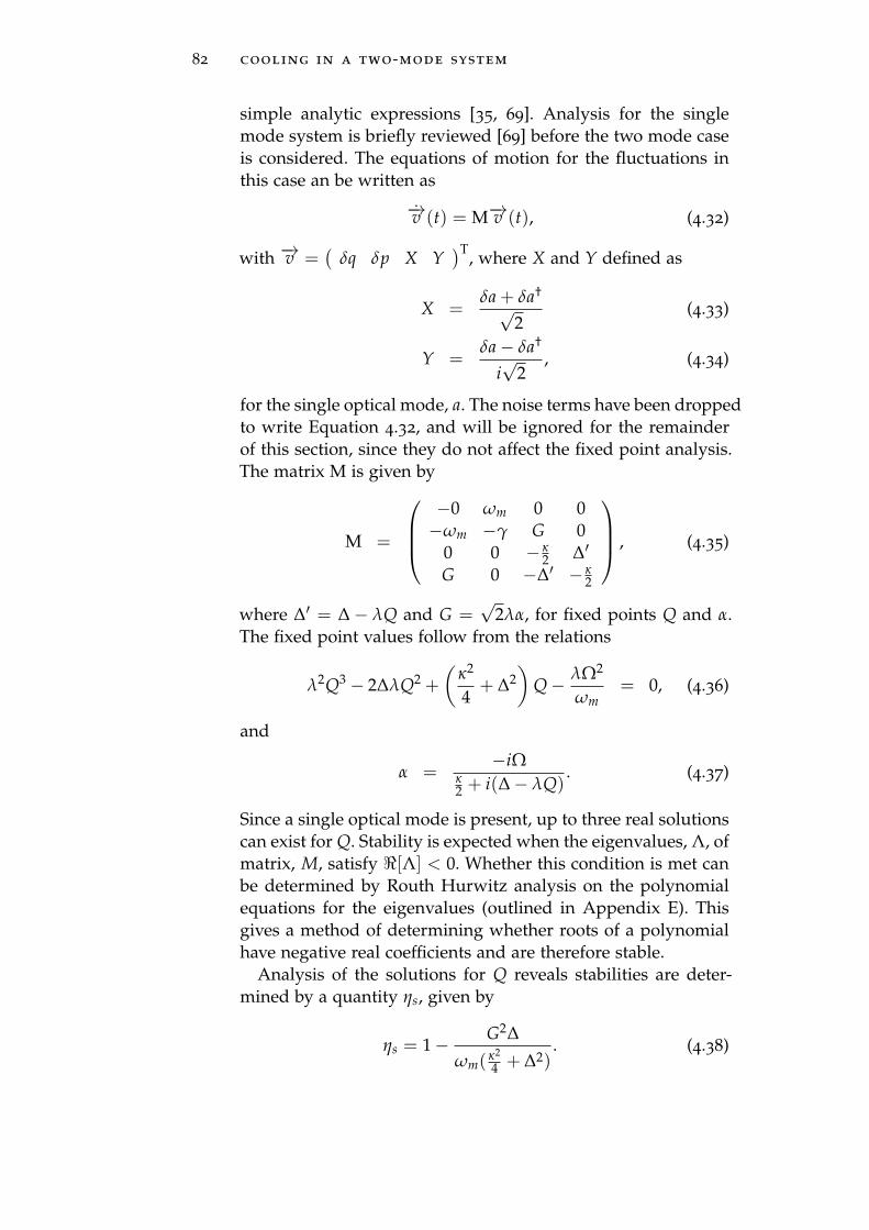
82 cooling in a two-mode system
simple analytic expressions [35, 69]. Analysis for the single
mode system is briefly reviewed [69] before the two mode case
is considered. The equations of motion for the fluctuations in
this case an be written as
−→v (t) = M−→v (t), (4.32)
with −→v =(
δq δp X Y)T
, where X and Y defined as
X =δa + δa†
√2
(4.33)
Y =δa− δa†
i√
2, (4.34)
for the single optical mode, a. The noise terms have been dropped
to write Equation 4.32, and will be ignored for the remainder
of this section, since they do not affect the fixed point analysis.
The matrix M is given by
M =
−0 ωm 0 0
−ωm −γ G 0
0 0 − κ2 ∆′
G 0 −∆′ − κ2
, (4.35)
where ∆′ = ∆− λQ and G =√
2λα, for fixed points Q and α.
The fixed point values follow from the relations
λ2Q3 − 2∆λQ2 +
(
κ2
4+ ∆2
)
Q− λΩ2
ωm= 0, (4.36)
and
α =−iΩ
κ2 + i(∆− λQ)
. (4.37)
Since a single optical mode is present, up to three real solutions
can exist for Q. Stability is expected when the eigenvalues, Λ, of
matrix, M, satisfy ℜ[Λ] < 0. Whether this condition is met can
be determined by Routh Hurwitz analysis on the polynomial
equations for the eigenvalues (outlined in Appendix E). This
gives a method of determining whether roots of a polynomial
have negative real coefficients and are therefore stable.
Analysis of the solutions for Q reveals stabilities are deter-
mined by a quantity ηs, given by
ηs = 1− G2∆
ωm(κ2
4 + ∆2). (4.38)

4.3 static bistability 83
When this quantity lies in the range 0 < ηs < 1, the solution Q
is stable[35, 69]. Figure 4.5 details the results of stability analy-
sis in the single mode case. When a static bistability arises, the
curve forms three branches, with the upper and lower branches
representing stable solutions and the central branch represent-
ing unstable solutions. This is illustrated by the solutions, Q,
together with their corresponding ηs values.
Ω
Q
33 34 3520
40
60
80
100
Ω33 34 35
0
-0.4
0.4
0.8
ηs
(a) (b)
Figure 4.5: Stability analysis for the single mode case: (a) Real solu-
tions to Q and (b) the bistability parameter ηs for the so-
lutions. In regions of bistability, solutions for Q lie on one
of three branches of a curve. The stable solutions lie along
the upper and lower branches (where 0 < η < 1), with
the central branch being unstable - this corresponds to
the negative branch of ηs. Parameters used are ωm = 0.5,
∆ = 2ωm, λ = 0.01, κ = 1 and γ = 10−4.
4.3.1.2 Double mode case
Returning to the case of two optical modes, a more detailed
account of the Routh Hurwitz analysis for solutions to Equation
4.25 follows. Defining the following variables,
XL(R) =δaL(R) + δa†
L(R)√2
(4.39)
YL(R) =δaL(R) − δa†
L(R)√2
(4.40)
(4.41)
a similar matrix equation for Equations 4.16 to 4.19 is written:
~v(t) = M~v(t), (4.42)

84 cooling in a two-mode system
for vector~v(t)T =(
XL(t) YL(t) XR(t) YR(t) δq δp)
, where
the matrix M is given by
M =
− κ2 ∆′L 0 g G′L 0
−∆′L − κ2 −g 0 GL 0
0 g − κ2 ∆′R −G′R 0
−g 0 −∆′R − κ2 −GR 0
0 0 0 0 0 ωm
GL −G′L −GR G′R −ωm −γ
, (4.43)
and the following are defined by the fixed point values,
G+L(R)
= λαL(R) + α∗
L(R)√2
(4.44)
G−L(R)
= iλαL(R) − α∗
L(R)√2
(4.45)
Note that the fixed point variables have an implicit Q depen-
dence. Stability is again determined by the eigenvalues, Λ, of
the matrix M. Solving for these gives
|M−Λ| = 0. (4.46)
Recall that ∆′L and ∆′R are functions of Q, so that there exists
a different matrix for each branch of the curve in Figure 4.3a.
Solving the eigenvalue problem, a sixth order polynomial is
obtained to determine Λ:
a6Λ6 + a5Λ5 + a4Λ4 + a3Λ3 + a2Λ2 + a1Λ + a0 = 0, (4.47)
where the coefficients are given by
a6 = 1 (4.48)
a5 = 2κ +γ
2(4.49)
a4 = a + κ(κ + 2γ) (4.50)
a3 = κa + γb + κ(
ω2m + κγ
)
(4.51)
a2 = κγb + κ2ω2m + β + ǫ (4.52)
a1 = κβ + γǫ (4.53)
a0 = ω2mǫ− 2λ2ωm|αL|2χL − 2λ2ωm|αR|2χr
+ωmgλ2 (α∗RαL + α∗LαR) χ1, (4.54)

4.3 static bistability 85
with
a = 2g2 + ω2m +
κ2
2+ (∆′L)
2 + (∆′R)2, (4.55)
b = a−ω2m (4.56)
β = 2ωmλ2[
g (α∗LαR + α∗RαL)− ∆′L|αL|2 − ∆′R|αR|2]
+ω2m, (4.57)
ǫ =κ4
16+
κ2
4
(
(∆′L)2 + (∆′R)
2)
+ (∆′L∆′R − g2)2
+κ2
2g2, (4.58)
χL = ∆′L(∆′R)
2 + 4γ2∆′L − g2∆′R (4.59)
χR = ∆′R(∆′L)
2 + 4γ2∆′R − g2∆′L (4.60)
χ1 = 2g(g2 − ∆′L∆′R + γ2). (4.61)
With a different polynomial in Equation 4.47 for each set of
fixed points, one must apply the Routh-Hurwitz analysis to
each set in turn (or each branch of the curve). For a stable set
of fixed points, the polynomial in Equation 4.47 has 6 solutions,
each with a negative real part, so that ~v(t) decays with time.
The first condition of the Routh-Hurwitz criterion requires
the coefficients an (where 0 ≤ n ≤ 6) be the same sign. This is
satisfied when ηd > 0, where ηd is defined
ηd=1− λ2(
2χL|αL|2 + 2χR|αR|2 − χ1g (α∗LαR + α∗RαL))
ωmǫ. (4.62)
This is the bistability parameter for the system, which falls in
the range 0 < ηd < 1, for the red detuned regime (∆′L, ∆′R > 0),
when the fixed point solution is stable.
The second condition requires that the first column of the
Routh Array (see Appendix E) contains no sign changes be-
tween elements. Whereas in the single mode case it is found
that 0 < ηs < 1 is sufficient to ensure the first and second
criteria are satisfied, the two mode case is more complicated.
When moving from an eigenvalue equation for a 4× 4 matrix
to a 6× 6 matrix, the eigenvalue analysis rapidly becomes more
complicated.
This second condition is examined in Table E.2 of Appendix
E. The first column contains six elements, labelled a6, a5, b1, c1,
d1, e1 and f1. Equation 4.48 shows a6 > 0, and it is simple to
show that f1 = a0. Full expressions for elements b1, c1, d1 and e1
are cumbersome, and not very illuminating, thus will be omit-
ted from this thesis. Suffice to say, whilst b1 > 0 for the red

86 cooling in a two-mode system
detuned regime, it cannot be guaranteed via analytic expres-
sions that the rest are positive when 0 < ηd < 1, ∆′L, ∆′R > 0.
That said, numerical evaluation of these elements over a range
of parameters suggests they are indeed positive for the condi-
tions mentioned, suggesting 0 < ηd < 1 as the sole condition
on stability. However, a full analytic proof of this remains to be
found.
Figure 4.6a shows the bistability parameter, ηd, for the fixed
point solutions plotted in Figure 4.3a. The graph comprises
three branches, where ηd < 0 corresponds to the unstable branch,
shown by a dashed line. Applying the remainder of the Routh
Hurwitz criteria confirms that the two branches where ηd > 0
satisfy the stability criteria, up until ηd = 1, where the system
transitions to a limit cycle. These results are consistent with the
results deduced from the potential V(q). As Figure 4.2 shows,
the positions of minima in the potential correspond to cases
where 0 < ηd < 1, whilst the maximum corresponds to ηd < 0.
The Routh Hurwitz analysis, however, is more systematic and
allows the behaviour of the fixed points to be observed more
clearly as parameters are varied.
Ω
ηd
(a) (b)
33 34 35 36−0.4
0.8
0.4
0
1.2
33 34 350.2
0.8
0.4
0.6
1
Ω
Ωa Ωb Ω0
Q
36
Figure 4.6: For solutions shown in Figure 4.3a, stability is demon-
strated via (a) the stability parameter, ηd, defined in Equa-
tion 4.62, and (b) a hysteresis curve, showing the fixed
points reached as the driving strength is swept up and
down, as indicated by arrows along the separate branches.
The vertical dotted lines in (a) mark Ω values which pro-
duce the potentials in corresponding colours in Figure 4.2,
as well as the onset of instability at Ω0 (in black). In (b),
the instability is marked alongside Ωa (cyan) and Ωb (ma-
genta) which mark the points where the systems switches
between fixed points as the drive strength is reduced and
increased, respectively.
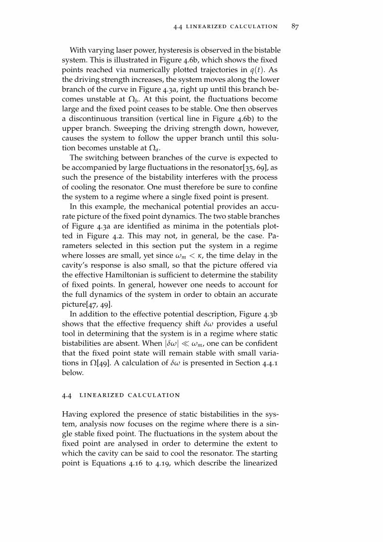
4.4 linearized calculation 87
With varying laser power, hysteresis is observed in the bistable
system. This is illustrated in Figure 4.6b, which shows the fixed
points reached via numerically plotted trajectories in q(t). As
the driving strength increases, the system moves along the lower
branch of the curve in Figure 4.3a, right up until this branch be-
comes unstable at Ωb. At this point, the fluctuations become
large and the fixed point ceases to be stable. One then observes
a discontinuous transition (vertical line in Figure 4.6b) to the
upper branch. Sweeping the driving strength down, however,
causes the system to follow the upper branch until this solu-
tion becomes unstable at Ωa.
The switching between branches of the curve is expected to
be accompanied by large fluctuations in the resonator[35, 69], as
such the presence of the bistability interferes with the process
of cooling the resonator. One must therefore be sure to confine
the system to a regime where a single fixed point is present.
In this example, the mechanical potential provides an accu-
rate picture of the fixed point dynamics. The two stable branches
of Figure 4.3a are identified as minima in the potentials plot-
ted in Figure 4.2. This may not, in general, be the case. Pa-
rameters selected in this section put the system in a regime
where losses are small, yet since ωm < κ, the time delay in the
cavity’s response is also small, so that the picture offered via
the effective Hamiltonian is sufficient to determine the stability
of fixed points. In general, however one needs to account for
the full dynamics of the system in order to obtain an accurate
picture[47, 49].
In addition to the effective potential description, Figure 4.3b
shows that the effective frequency shift δω provides a useful
tool in determining that the system is in a regime where static
bistabilities are absent. When |δω| ≪ ωm, one can be confident
that the fixed point state will remain stable with small varia-
tions in Ω[49]. A calculation of δω is presented in Section 4.4.1
below.
4.4 linearized calculation
Having explored the presence of static bistabilities in the sys-
tem, analysis now focuses on the regime where there is a sin-
gle stable fixed point. The fluctuations in the system about the
fixed point are analysed in order to determine the extent to
which the cavity can be said to cool the resonator. The starting
point is Equations 4.16 to 4.19, which describe the linearized

88 cooling in a two-mode system
dynamics[16] of the system with small fluctuations about its
mean field values.
The calculation proceeds by solving the system of Equations
(4.16 to 4.19) to obtain the spectrum of the resonator’s posi-
tion fluctuations. By comparing this spectrum with that of a
damped harmonic oscillator in thermal equilibrium, with a bath
at a given temperature T, an effective frequency, damping rate
and temperature can be deduced for a resonator coupled to a
two mode cavity system. The following analysis focuses on the
back action of the cavity on the resonator, as such the effects of
the thermal bath are ignored, and the damping, γ, and thermal
fluctuations, ζ, are dropped in Equations 4.16 and 4.17.
The symmetrised spectrum of position fluctuations is defined
as
Sq(ω) =1
2π
∫ ∞
−∞dte−iωt [〈δq(t)δq(0)〉+ 〈δq(0)δq(t)〉] . (4.63)
For an oscillator with frequency ω0, damped at a rate γ which
is in contact with a bath at temperature T, it is known that[71]
Sq(ω) =1
2π
(2n + 1)ωωmγ
(ω2 −ω2m)
2 + γ2ω2, (4.64)
where n = [eω
kBT − 1]−1. For a weakly damped system (γ ≪ωm) Sq(ω) is strongly peaked about ω = ωm and the thermal
occupation can be approximated as n = [eωm/kBT− 1]−1. Noting
that 〈δq2〉 = n + 12 , the spectrum can be written
Sq(ω) ≈ 1
2π
2ω2m〈δq2〉γ
(ω2 −ω2m)
2 + γ2ω2. (4.65)
The denominator in Equation 4.65 can be written as
|dwq|2 = |ω2 −ω2m + iγω|2. (4.66)

4.4 linearized calculation 89
4.4.1 Effective damping of the mechanical mode
Analysis of the mechanical fluctuations proceeds by Fourier
transforming Equations 4.16 to 4.19
δq(ω) =ωmλ
ω2 −ω2m
[
α∗RδaR(ω) + αRδa†R(ω)− α∗LδaL(ω)
−αLδa†R(ω)
]
(4.67)
δp(ω) =iω
ωmδq(ω) (4.68)
δaL(ω) = [hL(ω)]−1[
iλαLδq(ω)− igδaR(ω) +√
κaINL
]
(4.69)
δaR(ω) = [hR(ω)]−1[
−iλαRδq(ω)− igδaL(ω) +√
κaINR
]
(4.70)
where
hL(R) =κ
2+ i(
ω + ∆′L(R)
)
. (4.71)
Some rearranging decouples equations 4.67 to 4.70, giving an
expression for δq(ω) of the form
δq(ω) =ωmλ
A′(ω)
[
D1(ω)B2(ω)aINL + D2(ω)B1(ω)aIN†
L
+E1(ω)B2(ω)aINR + E2(ω)B1(ω)aIN†
R
]
, (4.72)
where the following are defined:
B1(ω) = hL(ω)hR(ω) + g2 (4.73)
B2(ω) = kL(ω)kR(ω) + g2 (4.74)
C1(ω) = −iλ[
|αL|2hR(ω) + |αR|2hL(ω)]
+gλ (α∗LαR + α∗RαL) (4.75)
C2(ω) = iλ[
|αR|2kL(ω) + |αL|2kR(ω)]
+gλ (αRα∗L + αLα∗R) (4.76)
D1(ω) = [igα∗R + α∗LhR(ω)]√
κ (4.77)
D2(ω) = [−igαR + αLkR(ω)]√
κ (4.78)
E1(ω) = − [α∗RhL(ω) + igα∗L]√
κ (4.79)
E2(ω) = − [αRkL(ω)− igαL]√
κ (4.80)
A(ω) =(
ω2 −ω2m
)
H(ω)K(ω) (4.81)
A′(ω) =ωmλ
−ωmλ [C1(ω)B2(ω) + C2(ω)B1(ω)]+A(ω)(4.82)

90 cooling in a two-mode system
where
kL(R) =κ
2+ i(
ω− ∆′L(R)
)
. (4.83)
The two point correlator 〈δq(ω)δq(ω′)〉 is then a sum of combi-
nations of aINL(R) and aIN†
L(R), of which Equations 4.8 and 4.9 give
the only non-zero contributions. The only non-zero correlators
follow from Equations 4.8 and 4.9:
〈aINL(R)(ω)aIN†
L(R)(ω′)〉 =
1
2πδ(ω + ω′). (4.84)
Picking out the two non-zero contributions, the 2 point corre-
lator, 〈δq(ω)δq(ω′)〉 is given by
〈δq(ω)δq(ω′)〉 = A′(ω)A′(ω′)2π
[
D1(ω)D2(ω′)B2(ω)B1(ω
′)
+E1(ω)E2(ω′)B2(ω)B1(ω
′)]
δ(ω + ω′).(4.85)
The spectrum is then found via Equation 4.63, where integrat-
ing over the delta functions amounts to setting ω′ = −ω. Anal-
ysis of the expressions given in Equations 4.73 to 4.82 reveals
B1(−ω) = B∗1(ω), and so on for each expression. This allows
the spectrum to be written as
Sq(ω)=(ωmλ)2
2π|dw(ω)|2 [F1(ω) + F2(ω)] , (4.86)
where the following are defined:
F1(2) =|D1(2)(ω)|2+|E1(2)(ω)|2
|B1(2)(ω)|2 (4.87)
dw(ω) = ω2 −ω2m + χ(ω), (4.88)
and
χ(ω) = ωmλ
[
C1(ω)
B1(ω)+
C2(ω)
B2(ω)
]
. (4.89)
A direct comparison can be made between dw(ω) and the de-
nominator in Equation 4.65. This allows an ‘effective’ damping
and frequency shift to be deduced, in analogy with the case of
the standard damped oscillator by identification
|dw(ω)|2 = |ω2 −ω2m + iγe f f ω|2. (4.90)

4.4 linearized calculation 91
The effective damping is therefore identified by extracting the
imaginary component of χ(ω),
γe f f (ω) =ωmλ
ωℑ[
C2
B2+
C1
B1
]
. (4.91)
With this expression in terms of ω, the approximation of a
weakly damped system is applied. Equation 4.65 was written
with the assumption that the spectrum is strongly peaked around
ωm. This same assumption allows the approximation ω = ωm
to be used to calculate a fixed value of γe f f :
γe f f (ω) = λℑ[
C2(ωm)
B2(ωm)+
C1(ωm)
B1(ωm)
]
. (4.92)
In general, however, there is a small frequency shift, so that the
spectrum is actually peaked about a value ωe f f , which relates
to the mechanical frequency by ωe f f = ωm + δω, where δω is
a small frequency shift. The frequency ωe f f can be identified
as the square root of the real component of χ(ωm) - taking the
frequency as ωm to make an initial calculation, which provides
a reasonable approximation when the shift is small, δω ≪ ωm:
ω2e f f = ω2
m + λℜ[
C2(ωm)
B2(ωm)+
C1(ωm)
B1(ωm)
]
. (4.93)
Given that δω ≪ ωm, the frequency shift can be approximated
ωe f f (ω) ≈ ωm +λ
2ℜ[
C1
B1+
C2
B2
]
, (4.94)
δω(ω) ≈ λ
2ℜ[
C1
B1+
C2
B2
]
. (4.95)
With regards to Equations 4.92 and 4.95, recall the assump-
tion of small fluctuations, which is required to linearize the
equations. The result is expressions for γe f f and δω which ap-
ply in the regime where the fixed point is stable. This allows
the regime of cooling to be investigated with these expressions.
One might also expect these expressions to accurately predict
the onset of instability. This will be addressed in the next chap-
ter. In the regime of limit cycles, amplitude dependent expres-
sions are expected, as in Chapters 2 and 3.
In the limit g→ 0, Equation 4.92 matches the case of a single
linearly coupled mode, for small energy (see Equation 2.76 of
Chapter 2). This is the linearized single mode result achieved
via a similar process by Genes et. al.[35].

92 cooling in a two-mode system
4.4.1.1 Numerical analysis
The effective damping is investigated by varying two param-
eters: the laser detuning, ∆, and the frequency shift arising
from the equilibrium displacement of the resonator, ∆ω. These
two parameters navigate the dispersion diagram of Figure 4.1,
bringing the system into resonance with the various modes
shown. This determines the interplay between optical and me-
chanical modes. Colour plots in figures 4.7a and 4.7c show the
behaviour of γe f f under different circumstances of note. There
are two distinct scenarios to consider, in terms of parameters
chosen:
• ωm < 2g - interactions between quadratic modes are weak
and the energy gap is too large for transitions between
modes. The behaviour of the system is similar to that of
the single mode case.
• ωm > 2g - interactions between quadratic modes are strong
and there exists a value of ∆ω where the energy gap be-
tween modes matches the mechanical frequency, so that
transitions between upper and lower bands are stimulated
by the absorption or emission of a phonon.
The optical modes are displayed as white dashed lines along-
side the damping, to illustrate how the proximity to optical
resonances affects the resonator motion. Also shown are the
modes shifted by the mechanical frequency.
The effective damping for the case where ωm < 2g is shown
in Figure 4.7a. The resonator is most strongly driven and damped
when the cavity is driven close to the quadratic mode frequen-
cies, resulting in features along the quadratic dispersion curves.
Strong anti-damping (negative values for the effective damp-
ing) occurs when the cavity is driven just above an optical fre-
quency, whilst strong damping occurs just below. Since the left
mode is driven directly by radiation, the features are stronger
when the dispersion curve (frequencies ω1,2) approaches the
driven mode (frequency ωL). This occurs along lines where the
mode frequencies coincide with −∆ = ∆ω.
Figure 4.7c shows the damping for a small energy gap, ωm >
2g. The dispersion curves and sidebands, shown in white, illus-
trate where the Stokes and anti-Stokes resonances occur[49, 16].
The form of the graph is distinctly different to Figure 4.7a; fea-
tures do not lie along the entirety of the dispersion curves
but are confined to regions where the curves cross. Here the

4.4 linearized calculation 93
system moves between optical modes by exchanging mechan-
ical quanta: ωm = ω1 − ω2. The energy exchange is stronger
near the driven mode. The result is a graph with features at
A - where emission from the cavity causes driving (γe f f < 0)
- and B - where the cavity absorbs energy, causing damping
(γe f f > 0).
−20
0
20
−200
0
×10−4
∆ω
−∆
γe
ff
20
−2
2
(a)
−20
0
20
−200
0
×10−7
∆ω−
∆
δωe
ff
20
−4
4
(b)
−5
0
5
−50
0
×10−4
∆ω
−∆
γe
ff
−1
1
5
A
B
(c)
−5
0
5
−50 5
5
−5
0
×10−7
∆ω
−∆
δωe
ff
A
B
(d)
Figure 4.7: Effective damping and frequency shift in the resonator,
with respect to ∆ and ∆ω, for two different regimes: (a)
and (b) show γe f f and δω for g = 10 and ωm = 0.5, where
the energy gap between the photon modes is large, and so
driving and damping occur when the cavity is driven just
above or below the quadratic modes. Figures (c) and (d)
show γe f f and δω for g = 1, ωm = 4, where a small en-
ergy gap results strong interactions at ωm = 2√
g2 + ∆ω2,
allowing transitions between photon modes. The remain-
ing parameters are Ω = 1 and λ = 10−2 in both cases.
Figures 4.7d and 4.7b show the frequency shift in the res-
onator, deduced in Equation 4.95. Since the shift doesn’t be-
come any larger than ∆ω ∼ 10−4, the resonator dynamics lies
well within the range ∆ω ≪ ωm, so that the static bistability is
unlikely to cause an issue.
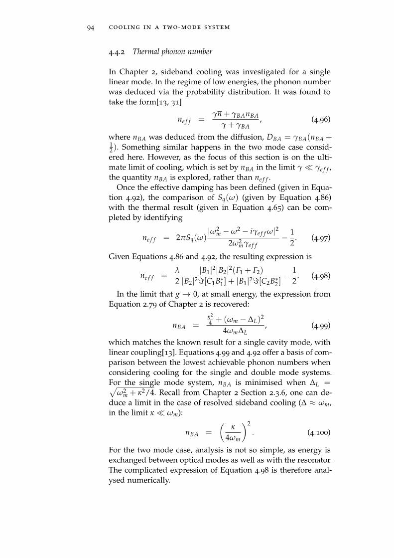
94 cooling in a two-mode system
4.4.2 Thermal phonon number
In Chapter 2, sideband cooling was investigated for a single
linear mode. In the regime of low energies, the phonon number
was deduced via the probability distribution. It was found to
take the form[13, 31]
ne f f =γn + γBAnBA
γ + γBA, (4.96)
where nBA was deduced from the diffusion, DBA = γBA(nBA +12). Something similar happens in the two mode case consid-
ered here. However, as the focus of this section is on the ulti-
mate limit of cooling, which is set by nBA in the limit γ≪ γe f f ,
the quantity nBA is explored, rather than ne f f .
Once the effective damping has been defined (given in Equa-
tion 4.92), the comparison of Sq(ω) (given by Equation 4.86)
with the thermal result (given in Equation 4.65) can be com-
pleted by identifying
ne f f = 2πSq(ω)|ω2
m −ω2 − iγe f f ω|22ω2
mγe f f− 1
2. (4.97)
Given Equations 4.86 and 4.92, the resulting expression is
ne f f =λ
2
|B1|2|B2|2(F1 + F2)
|B2|2ℑ[C1B∗1 ] + |B1|2ℑ[C2B∗2 ]− 1
2. (4.98)
In the limit that g → 0, at small energy, the expression from
Equation 2.79 of Chapter 2 is recovered:
nBA =κ2
4 + (ωm − ∆L)2
4ωm∆L, (4.99)
which matches the known result for a single cavity mode, with
linear coupling[13]. Equations 4.99 and 4.92 offer a basis of com-
parison between the lowest achievable phonon numbers when
considering cooling for the single and double mode systems.
For the single mode system, nBA is minimised when ∆L =√
ω2m + κ2/4. Recall from Chapter 2 Section 2.3.6, one can de-
duce a limit in the case of resolved sideband cooling (∆ ≈ ωm,
in the limit κ ≪ ωm):
nBA =
(
κ
4ωm
)2
. (4.100)
For the two mode case, analysis is not so simple, as energy is
exchanged between optical modes as well as with the resonator.
The complicated expression of Equation 4.98 is therefore anal-
ysed numerically.
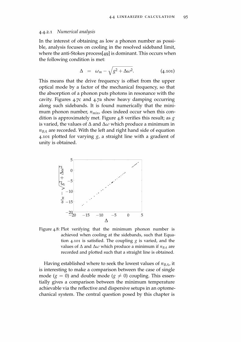
4.4 linearized calculation 95
4.4.2.1 Numerical analysis
In the interest of obtaining as low a phonon number as possi-
ble, analysis focuses on cooling in the resolved sideband limit,
where the anti-Stokes process[49] is dominant. This occurs when
the following condition is met:
∆ = ωm −√
g2 + ∆ω2. (4.101)
This means that the drive frequency is offset from the upper
optical mode by a factor of the mechanical frequency, so that
the absorption of a phonon puts photons in resonance with the
cavity. Figures 4.7c and 4.7a show heavy damping occurring
along such sidebands. It is found numerically that the mini-
mum phonon number, nmin, does indeed occur when this con-
dition is approximately met. Figure 4.8 verifies this result; as g
is varied, the values of ∆ and ∆ω which produce a minimum in
nBA are recorded. With the left and right hand side of equation
4.101 plotted for varying g, a straight line with a gradient of
unity is obtained.
ωm−√
g2+
∆ω
2
∆
−20
−15
−10
−5
0
5
−20 −15 −10 −5 0 5
Figure 4.8: Plot verifying that the minimum phonon number is
achieved when cooling at the sidebands, such that Equa-
tion 4.101 is satisfied. The coupling g is varied, and the
values of ∆ and ∆ω which produce a minimum if nBA are
recorded and plotted such that a straight line is obtained.
Having established where to seek the lowest values of nBA, it
is interesting to make a comparison between the case of single
mode (g = 0) and double mode (g 6= 0) coupling. This essen-
tially gives a comparison between the minimum temperature
achievable via the reflective and dispersive setups in an optome-
chanical system. The central question posed by this chapter is

96 cooling in a two-mode system
whether or not it is possible to achieve temperatures as low as
in the reflective case by using the dispersive system, which of-
fers a much simpler method of fabrication. The parameter Nmin
is therefore defined, for use within this section:
Nmin(g) =nmin(g)
nmin(g = 0). (4.102)
The minimum achievable phonon number is investigated for
varying tunnelling rate, g. Equation 4.100 suggests that increas-
ing ωm will reduce the minimum phonon number for the single
mode case, so that cooling is more effective in the resolved side-
band limit[13]. Figure 4.9 verifies this, showing that nBA ≪ 1 as
the resolved sideband limit is approached, for Ω = 1, λ = 10−2,
κ = 1.
0
0.01
0.02
0.03
0.04
0.05
0.06
2 4 6 8 10 12 14
nB
A
ωm
21.20.8 1.60.40
0.2
0.4
0.6
0.8
1
Figure 4.9: Minimum effective phonon number for the single mode
case (solid) for varying ωm, plotted alongside Equation
4.100 (dashed). The inset shows where the curves begin
to diverge in the bad cavity limit. At each value of ωm,
nBA is calculated for ∆ =√
ω2m + κ2/4. The remaining
parameters are Ω = 1, λ = 10−2, κ = 1.
Turning to the case where g 6= 0, Figure 4.10 shows the quan-
tity Nm for the resolved sideband regime, as g is varied. The
ratio generally remains close to 1, with the exception of a peak
which occurs in the vicinity of ωm = g, increasing in magnitude
as ωm and g increase.
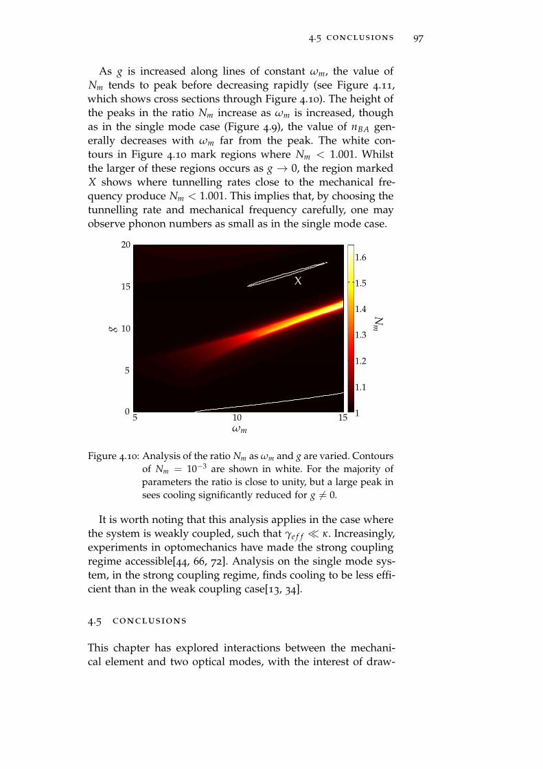
4.5 conclusions 97
As g is increased along lines of constant ωm, the value of
Nm tends to peak before decreasing rapidly (see Figure 4.11,
which shows cross sections through Figure 4.10). The height of
the peaks in the ratio Nm increase as ωm is increased, though
as in the single mode case (Figure 4.9), the value of nBA gen-
erally decreases with ωm far from the peak. The white con-
tours in Figure 4.10 mark regions where Nm < 1.001. Whilst
the larger of these regions occurs as g → 0, the region marked
X shows where tunnelling rates close to the mechanical fre-
quency produce Nm < 1.001. This implies that, by choosing the
tunnelling rate and mechanical frequency carefully, one may
observe phonon numbers as small as in the single mode case.
0
5
10
15
20
5 10 15ωm
g
1
1.1
1.2
1.3
1.5
1.4
1.6
Nm
X
Figure 4.10: Analysis of the ratio Nm as ωm and g are varied. Contours
of Nm = 10−3 are shown in white. For the majority of
parameters the ratio is close to unity, but a large peak in
sees cooling significantly reduced for g 6= 0.
It is worth noting that this analysis applies in the case where
the system is weakly coupled, such that γe f f ≪ κ. Increasingly,
experiments in optomechanics have made the strong coupling
regime accessible[44, 66, 72]. Analysis on the single mode sys-
tem, in the strong coupling regime, finds cooling to be less effi-
cient than in the weak coupling case[13, 34].
4.5 conclusions
This chapter has explored interactions between the mechani-
cal element and two optical modes, with the interest of draw-
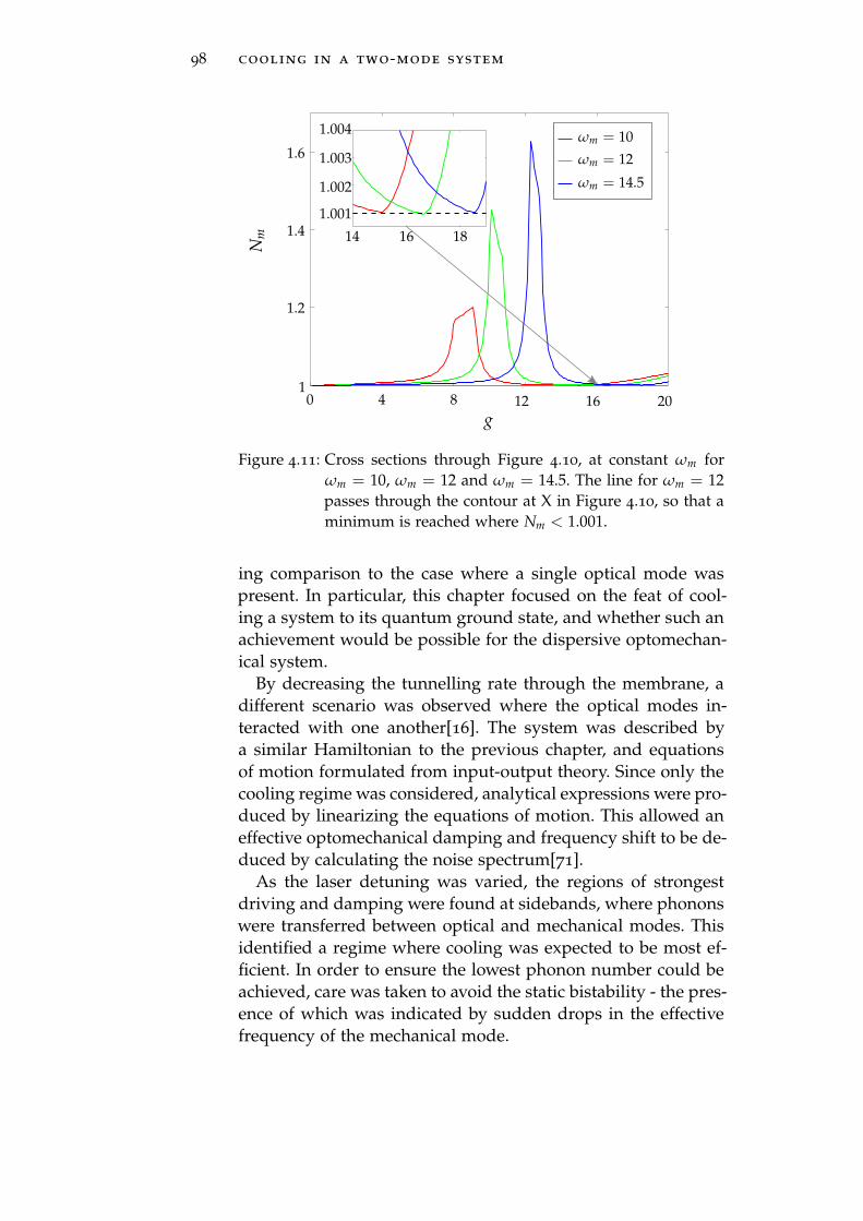
98 cooling in a two-mode system
1
1.2
1.4
1.6
0 4 8 12 16 20
g
Nm
1.001
1.002
1.003
1.004
14 16 18
ωm = 10
ωm = 12
ωm = 14.5
Figure 4.11: Cross sections through Figure 4.10, at constant ωm for
ωm = 10, ωm = 12 and ωm = 14.5. The line for ωm = 12
passes through the contour at X in Figure 4.10, so that a
minimum is reached where Nm < 1.001.
ing comparison to the case where a single optical mode was
present. In particular, this chapter focused on the feat of cool-
ing a system to its quantum ground state, and whether such an
achievement would be possible for the dispersive optomechan-
ical system.
By decreasing the tunnelling rate through the membrane, a
different scenario was observed where the optical modes in-
teracted with one another[16]. The system was described by
a similar Hamiltonian to the previous chapter, and equations
of motion formulated from input-output theory. Since only the
cooling regime was considered, analytical expressions were pro-
duced by linearizing the equations of motion. This allowed an
effective optomechanical damping and frequency shift to be de-
duced by calculating the noise spectrum[71].
As the laser detuning was varied, the regions of strongest
driving and damping were found at sidebands, where phonons
were transferred between optical and mechanical modes. This
identified a regime where cooling was expected to be most ef-
ficient. In order to ensure the lowest phonon number could be
achieved, care was taken to avoid the static bistability - the pres-
ence of which was indicated by sudden drops in the effective
frequency of the mechanical mode.
4.5 conclusions 99
Cooling was investigated by deducing the effective phonon
number via the mechanical noise spectrum. By varying the tun-
nelling rate, the efficiency of cooling was compared between
single and double mode systems. It was found that there ex-
isted combinations of g 6= 0 and ωm which produce effective
phonon numbers within 0.1% of the lowest achievable phonon
number, in the single mode case. The conclusion drawn is that
allowing radiation to pass through the membrane can produce
cooling effects as efficient in the red detuned regime. This pro-
vides a possible method of cooling an oscillator to its quantum
ground state, whilst overcoming the issue of fabricating highly
reflective elements with a high mechanical quality factor[17].


5T W O M O D E D Y N A M I C S : F R O M L I M I T C Y C L E S
T O C H A O S
5.1 introduction
Previously, the driven non-linear regime has been explored for
systems where single optical modes are coupled linearly and
quadratically to the mechanical mode. In these cases, the non-
linear dynamics and quantum fluctuations have been explored
with a combination of numerical and analytic calculations. Fur-
ther to this, Chapter 4 explored the linear dynamics of the sys-
tem when two optical modes were present, in the red detuned
regime. This chapter progresses by exploring the two optical
mode system for the case of blue detuning. However, the pres-
ence of three harmonic oscillators results in a more complex
system, and analysis for this system is more difficult than for
those studied in Chapters 2 and 3.
Owing to the complexity of the two optical mode system,
analysis of this chapter focuses on the average dynamics of the
system. This is made possible by exploring the regime of strong
driving, where the system is driven to large amplitude oscilla-
tions, and fluctuations become less important. The dynamics of
the resulting limit cycles will be explored, as well as the tran-
sition to chaos. Numerical analysis explores the trajectory of
variables characterising the system, comparing the long time
behaviour as the mechanical coupling is swept. An analytical
calculation is presented in the form of a rotating wave approx-
imation on the photon mode equations, allowing a description
of the limit cycle dynamics.
This chapter is organised as follows. In section 5.2 the two
mode driven system is introduced, and the equations of mo-
tion deduced. Section 5.3 presents a numerical analysis of the
equations, first addressing the case where the drive is provided
by a thermal bath, before exploring the case where the system
is driven by a laser source. The dynamics are mapped out over
the blue detuned range. Section 5.4 presents an analytical cal-
culation of the limit cycle amplitudes in the regime where pe-
riodic oscillations occur, for weaker coupling strengths. This is
achieved via a rotating wave approximation. The predictions
101
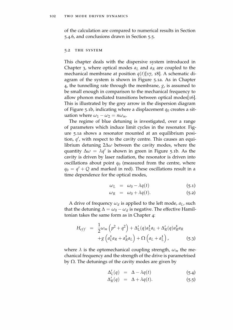
102 two mode driven dynamics
of the calculation are compared to numerical results in Section
5.4.6, and conclusions drawn in Section 5.5.
5.2 the system
This chapter deals with the dispersive system introduced in
Chapter 3, where optical modes aL and aR are coupled to the
mechanical membrane at position q(t)[17, 18]. A schematic di-
agram of the system is shown in Figure 5.1a. As in Chapter
4, the tunnelling rate through the membrane, g, is assumed to
be small enough in comparison to the mechanical frequency to
allow phonon mediated transitions between optical modes[16].
This is illustrated by the grey arrow in the dispersion diagram
of Figure 5.1b, indicating where a displacement q0 creates a sit-
uation where ω1 −ω2 = nωm.
The regime of blue detuning is investigated, over a range
of parameters which induce limit cycles in the resonator. Fig-
ure 5.1a shows a resonator mounted at an equilibrium posi-
tion, q′, with respect to the cavity centre. This causes an equi-
librium detuning 2∆ω between the cavity modes, where the
quantity ∆ω = λq′ is shown in green in Figure 5.1b. As the
cavity is driven by laser radiation, the resonator is driven into
oscillations about point q0 (measured from the centre, where
q0 = q′ + Q and marked in red). These oscillations result in a
time dependence for the optical modes,
ωL = ω0 − λq(t) (5.1)
ωR = ω0 + λq(t). (5.2)
A drive of frequency ωd is applied to the left mode, aL, such
that the detuning ∆ = ω0−ωd is negative. The effective Hamil-
tonian takes the same form as in Chapter 4:
He f f =1
2ωm
(
p2 + q2)
+ ∆′L(q)a†LaL + ∆′R(q)a†
RaR
+g(
a†LaR + a†
RaL
)
+ Ω(
aL + a†L
)
, (5.3)
where λ is the optomechanical coupling strength, ωm the me-
chanical frequency and the strength of the drive is parametrised
by Ω. The detunings of the cavity modes are given by
∆′L(q) = ∆− λq(t) (5.4)
∆′R(q) = ∆ + λq(t). (5.5)
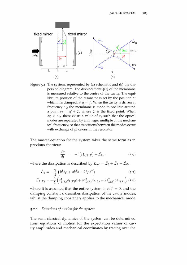
5.2 the system 103
L
q(t)
fixed mirror fixed mirror
L
ωD
q = 0
q′ Q
q0
(a)
q
ωca
v
ωR
ωL
nωm
q0
ω1
ω2
2g ∆ωq′
(b)
Figure 5.1: The system, represented by (a) schematic and (b) the dis-
persion diagram. The displacement q(t) of the membrane
is measured relative to the centre of the cavity. The equi-
librium position of the resonator is set by the position at
which it is clamped, at q = q′. When the cavity is driven at
frequency ωd the membrane is made to oscillate around
a point q0 = q′ + Q, where Q is the fixed point. When
2g < ωm there exists a value of q0 such that the optical
modes are separated by an integer multiple of the mechan-
ical frequency, so that transitions between the modes occur
with exchange of phonons in the resonator.
The master equation for the system takes the same form as in
previous chapters:
dρ
dt= −i
[
He f f , ρ]
+ Ltot, (5.6)
where the dissipation is described by Ltot = Lb + LL + LR:
Lb = −γ
2
(
b†bρ + ρb†b− 2bρb†)
(5.7)
LL(R) =−κ
2
(
a†L(R)aL(R)ρ + ρa†
L(R)aL(R) − 2a†L(R)ρaL(R)
)
, (5.8)
where it is assumed that the entire system is at T = 0, and the
damping constant κ describes dissipation of the cavity modes,
whilst the damping constant γ applies to the mechanical mode.
5.2.1 Equations of motion for the system
The semi classical dynamics of the system can be determined
from equations of motion for the expectation values of cav-
ity amplitudes and mechanical coordinates by tracing over the

104 two mode driven dynamics
master equation (Equation 5.6)[1] - For example, the average oc-
cupation of the left cavity mode, 〈aL〉 = αL obeys the equation
αL = Tr [aLρ] (5.9)
= −[
i∆′L(q) +κ
2
]
αL − igαR − iΩ. (5.10)
Similarly, equations of motion are obtained for the average dy-
namics of the right cavity, αR, and membrane co-ordinates:
α∗L =[
i∆′L(q)−κ
2
]
α∗L + igα∗R + iΩ (5.11)
αR = −[
i∆′R(q) +κ
2
]
αR − igαL (5.12)
α∗R =[
i∆′R(q)−κ
2
]
α∗R + igα∗L. (5.13)
q = ωm p (5.14)
p = −ωmq− γp + λ(α∗LαL − α∗RαR), (5.15)
where the semi classical approximation a†LaL = α∗LαL and a†
RaR =α∗RαR is made in the last line.
5.3 numerical analysis
When the laser drive is blue detuned so that the system is
driven, Equations 5.10 to 5.15 lead to a complex non-linear
dynamics. Aspects of this dynamics have been described pre-
viously in the literature[39, 40, 41, 42], and these approaches
are extended in the analysis to follow, starting with a straight
forward numerical calculation.
This chapter aims to explore this varied behaviour in the sys-
tem, in the regime of blue detuning. Equations 5.10 to 5.15 can-
not be solved exactly. Instead a numerical approach is taken, us-
ing a range of carefully selected parameters that allow one to ex-
plore the different behaviours that arise. The coupled equations
are solved directly, by numerical integration. The integration is
performed using the Adams-Bashforth-Moulton method [73].
This method lends itself well to the system of interest, given the
chaotic nature of the dynamics at high coupling. In contrast to
single step methods, every data point calculated is dependent
on four prior data points. This method allows one to calculate
the local truncation error and correct it, improving the accuracy.
This is a desirable property for a method dealing with chaotic
motion, where small deviations from the initial trajectory grow
exponentially with time[9, 49].

5.3 numerical analysis 105
The analysis in the rest of this section explores the evolution
of the mean field variables as λ is increased in an attempt to
map out the full dynamics of the driven system. For varying
parameters the system follows a complicated path, before set-
tling into one of 3 different long time behaviours; these are
1. Fixed point - decaying fluctuations,
2. Stable oscillations - limit cycles,
3. Chaos.
Numerical plots are made of the trajectory x(t), where q has
been shifted by the equilibrium displacement, so that x = q−q′.
5.3.1 Dynamics in the presence of a thermal bath
A recent publication investigated this same system numerically
[40], in the absence of a laser drive: Ω = 0. Instead a drive is
supplied in the form of a heat bath, by assuming the cavity is at
a finite temperature. This is described by a finite thermal occu-
pation number nth, which is assumed for the optical cavity. The
advantage of this is that the resulting Hamiltonian contains a
symmetry which can be exploited, by defining a photon deple-
tion number, y, and photon inversion number, z, in terms of the
initial photon number N0:
y =a†
LaL + a†RaR
N0(5.16)
z =a†
LaL − a†RaR
N0, (5.17)
and the phase, φ, determined by φ = arg(a†LaR). Formulating
the system in terms of these operators reduces the number of
equations required to describe the corresponding semi-classical
dynamics. The equations for the average values now take the
form
q = ωm p (5.18)
x = −ωmx− γp + λN0z (5.19)
z = 2g√
x2 − z2 sin φ− κ
2z (5.20)
φ = 2λx− 2gz√
y2 − z2cos φ (5.21)
y = −κ
2y +
2κnth
N0, (5.22)

106 two mode driven dynamics
instead of Equations 5.10 to 5.15. The first two equations de-
scribe a damped harmonic oscillator, driven by the term λN0z,
whilst the next two describe the motion of a pendulum of vary-
ing length, with a drive of 2λx. With numerical analysis of the
trajectories, one finds oscillations can only be sustained for the
case κ = γ = 0, where the dynamics are chaotic[40].
The presence of a non-zero cavity mode thermal occupation
(nth 6= 0) acts as an effective drive (instead of the Ω term in
Equations 5.10 to 5.15) but this is an unphysical scenario; as
explained in Chapter 2, the cavity occupation at room tempera-
ture is negligible. In order to generate nth = 100, as is used in
[40], the cavity would need to be at a significantly higher tem-
perature, whilst maintaining the resonator at zero temperature,
which is impractical.
5.3.2 Driven oscillations
Here the laser drive is included, and it is assumed that the cav-
ity thermal occupation can be neglected. The drive provides an
energy source, allowing for a variety of long time behaviours as
the optomechanical coupling is swept. These behaviours will be
mapped out, showing how they evolve as a function of the op-
tomechanical coupling, λ. The coupling determines the energy
exchange between the optical and mechanical modes, which de-
termines how strongly the resonator is driven. Table 5.1 details
the parameters selected to explore the system.
Table 5.1: Parameters for numerical analysis
Parameter value (units κ = 1)
ωm 2
Ω 10
g 0.1
∆ -1
∆ω 1
γ 0.01
n 0
Varying the coupling takes the system through a series of
transitions. Broadly speaking, four different regimes of behaviour
can be identified in the resonator, as the coupling is swept. The
weak coupling regime is dominated by the fixed point solution.
For the parameters of Table 5.1, a single stable fixed point is
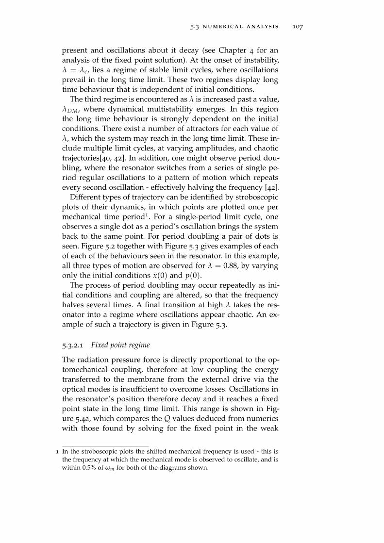
5.3 numerical analysis 107
present and oscillations about it decay (see Chapter 4 for an
analysis of the fixed point solution). At the onset of instability,
λ = λc, lies a regime of stable limit cycles, where oscillations
prevail in the long time limit. These two regimes display long
time behaviour that is independent of initial conditions.
The third regime is encountered as λ is increased past a value,
λDM, where dynamical multistability emerges. In this region
the long time behaviour is strongly dependent on the initial
conditions. There exist a number of attractors for each value of
λ, which the system may reach in the long time limit. These in-
clude multiple limit cycles, at varying amplitudes, and chaotic
trajectories[40, 42]. In addition, one might observe period dou-
bling, where the resonator switches from a series of single pe-
riod regular oscillations to a pattern of motion which repeats
every second oscillation - effectively halving the frequency [42].
Different types of trajectory can be identified by stroboscopic
plots of their dynamics, in which points are plotted once per
mechanical time period1. For a single-period limit cycle, one
observes a single dot as a period’s oscillation brings the system
back to the same point. For period doubling a pair of dots is
seen. Figure 5.2 together with Figure 5.3 gives examples of each
of each of the behaviours seen in the resonator. In this example,
all three types of motion are observed for λ = 0.88, by varying
only the initial conditions x(0) and p(0).The process of period doubling may occur repeatedly as ini-
tial conditions and coupling are altered, so that the frequency
halves several times. A final transition at high λ takes the res-
onator into a regime where oscillations appear chaotic. An ex-
ample of such a trajectory is given in Figure 5.3.
5.3.2.1 Fixed point regime
The radiation pressure force is directly proportional to the op-
tomechanical coupling, therefore at low coupling the energy
transferred to the membrane from the external drive via the
optical modes is insufficient to overcome losses. Oscillations in
the resonator’s position therefore decay and it reaches a fixed
point state in the long time limit. This range is shown in Fig-
ure 5.4a, which compares the Q values deduced from numerics
with those found by solving for the fixed point in the weak
1 In the stroboscopic plots the shifted mechanical frequency is used - this isthe frequency at which the mechanical mode is observed to oscillate, and iswithin 0.5% of ωm for both of the diagrams shown.
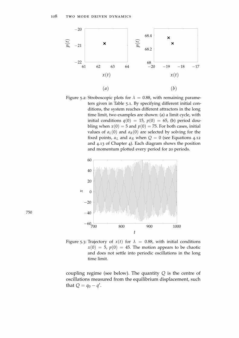
108 two mode driven dynamics
p(t)
−22
−21
−20
68.4
68.2
68
p(t)
x(t)
61 62 63 64 −20 −19 −18 −17
x(t)
(b)(a)
Figure 5.2: Stroboscopic plots for λ = 0.88, with remaining parame-
ters given in Table 5.1. By specifying different initial con-
ditions, the system reaches different attractors in the long
time limit, two examples are shown: (a) a limit cycle, with
initial conditions q(0) = 15, p(0) = 65, (b) period dou-
bling when x(0) = 5 and p(0) = 75. For both cases, initial
values of aL(0) and aR(0) are selected by solving for the
fixed points, αL and αR when Q = 0 (see Equations 4.12
and 4.13 of Chapter 4). Each diagram shows the position
and momentum plotted every period for 20 periods.
60
40
20
0
−60
−20
−40750
1000700 800 900
t
x
Figure 5.3: Trajectory of x(t) for λ = 0.88, with initial conditions
x(0) = 5, p(0) = 45. The motion appears to be chaotic
and does not settle into periodic oscillations in the long
time limit.
coupling regime (see below). The quantity Q is the centre of
oscillations measured from the equilibrium displacement, such
that Q = q0 − q′.

5.3 numerical analysis 109
At weak coupling, Q increases approximately linearly with
λ:
Q =λ
ωm
(
|αL|2 − |αR|2)
, (5.23)
where αL and αR can be approximated by
αL ≈−iΩ
[
κ2 + i∆R
]
[
κ2 + i∆R
] [
κ2 + i∆L
]
+ g2(5.24)
αR ≈ −gΩ[
κ2 + i∆R
] [
κ2 + i∆L
]
+ g2. (5.25)
where ∆L and ∆R are taken as Q independent:
∆L = ∆− ∆ω (5.26)
∆R = ∆ + ∆ω. (5.27)
Throughout this regime, the short time oscillations occur at ap-
proximately the mechanical frequency.
numerical data
0.1
0.2
0.05
0.15
0.25
Q
0.005 0.01 0.015 0.02λ
linear approx
λc
(a)
λ/λc
γe
ff
0 0.2 0.4 0.6 0.8 1 1.2
×10−3
−5
0
5
10
(b)
Figure 5.4: Fixed point dynamics (a) in stable regime, where oscilla-
tions decay - showing how Q varies with λ and (b) predic-
tion of the instability at λc = 0.0148, using the linearised
calculation of Chapter 4. The instability is predicted to oc-
cur when γe f f = γ + γBA = 0.
5.3.2.2 Limit cycle regime
As the coupling is increased, a value λc is approached, where
the work done via the radiation pressure force balances the dis-
sipation, and an instability occurs. In terms of the linearized
analysis of Chapter 4 this is where the (negative) back action
damping matches the intrinsic damping. Here oscillations are
sustained, and a limit cycle state becomes stable. At this point

110 two mode driven dynamics
the approximation in Equation 5.23 breaks down (as shown in
Figure 5.4a); Q is no longer linear with λ, and represents the
centre of stable oscillations. The linearized calculation of Chap-
ter 4 provides an accurate estimate of the onset of limit cycles.
This calculation is shown in Figure 5.4b.
Figure 5.5 shows how the limit cycle solutions evolve as λ is
increased. The dotted line marks λc = 0.0148, where a smooth
transition from fixed point to increasing amplitude oscillations
(at approximately ωm) occurs. The transition is continuous, in
that the amplitude, A, increases smoothly from A = 0. The
curve peaks around λ = 0.024, showing a smooth, steep in-
cline, before falling asymptotically towards A = 0. At λ = 0.12,
dynamical multistability occurs and multiple attractors begin
to emerge. Throughout this regime the oscillation frequency re-
mains close to the mechanical frequency.
As the coupling increases, the number of attractors increases.
The limit cycle amplitudes follow smooth curves at increasingly
higher amplitudes, which fall off asymptotically, never crossing
each other. As λ increases, the long time behaviour becomes
more sensitive to initial conditions. For a given limit cycle, the
range of initial conditions which produce the corresponding
trajectory then becomes very narrow.
For λ ≥ 0.87, period doubling and chaos are observed for
certain initial conditions. As λ increases, these behaviours occur
for a wider range of initial conditions, up to a point where
chaos appears to dominate the long time behaviour. The exact
value of λ at which the transition to chaotic behaviour occurs
has not been found. In order to determine it with any certainty,
one would need to map out a series of trajectories with varying
initial conditions in the six dimensional parameter space. This
is time consuming and it is not possible to ensure all possible
limit cycles have been eliminated, as some attractors may only
be approached from arbitrarily close to the trajectory.
Numerical analysis allows one to map out the dynamics of
the system over a range of optomechanical couplings ranging
from very weak (λ ≪ ωm) through to the strong coupling re-
gime (λ ∼ ωm). There are limitations to this method, however,
owing to the presence of dynamical multistability in the sys-
tem. With the presence of multiple trajectories, which can be
very sensitive to initial conditions, it is necessary to search for
different types of motion by shear brute force; sweeping initial
parameters through a range of values with the aim of picking
up all possible long time behaviours.

5.3 numerical analysis 111
A0
λ
λc 0.1 0.2 0.3 0.4
20
40
60
80
100
120
140
0.01 0.02 0.03 0.04 0.050
50
100
150
λDM
Figure 5.5: Amplitude of stable limit cycles, showing the onset of in-
stabilities (λc) and dynamical multistability (λDM) as ver-
tical dotted lines. Limit cycles are shown for a range of λ
values, and occur along a series of branches. Inset shows
a closeup of the weak coupling regime, where limit cycles
appear at λc = 0.0148.
Since the limit cycles lie along several smooth curves, a limit
cycle can usually be found at λ by selecting initial conditions
which lie along the trajectory of a limit cycle at λ− δλ, where
δλ≪ λ. This allows most curves to be completed once a couple
of points along the curve have been found. This method does
not, however, offer any certainty that all possible limit cycles
and chaotic or period-doubled trajectories have been identified.
In particular, the limit cycle curves have a start and end point,
towards which the limit cycle attractor becomes more difficult
to approach, unless an initial condition can be guessed close to,
or along, the trajectory of interest.
To offer a more systematic method of mapping out the dy-
namics, an analytic description of the system is sought. The
next section presents a calculation of the limit cycle amplitudes.
This will require a series of approximations, which limit analy-
sis to small λ values, such that λQ ≪ ∆ω. Whilst this approx-
imation is not valid for the entire range of Figure 5.5, it will
provide a systematic method of searching for limit cycles over
the weak coupling range.
112 two mode driven dynamics
5.4 analytic modelling of the limit cycle regimes
In this section the membrane motion is modelled by driven
oscillations about the fixed position q0 (as labelled in red in
figure 5.1a), at a fixed amplitude, A, and fixed frequency, ωm:
q(t) = q0 + A cos (ωmt), (5.28)
This ansatz is supported by the numerical analysis of Section
5.3, where the limit cycle regime sees regular oscillations at ap-
proximately the mechanical frequency. Prior studies also sup-
port this ansatz[13, 67]. By selecting fixed parameters q0, A and
ωm, one can search for periodic motion, seeking out parameters
which fit this ansatz. The approach taken in this section utilises
a similar method to that employed by Heinrich et. al.[67], ex-
tending the analysis to generalise the results.
Stable limit cycles occur when losses in the system are bal-
anced by the radiation pressure forces[37, 41]. This is the case
when the total damping in the system is zero. Applying this
condition gives an estimate of where limit cycles occur. This
requires an amplitude dependent expression for the damping
due to back action, which is expressed in terms of the cav-
ity mode operators. These will be deduced by writing down
a Schrodinger equation and applying a rotating wave approxi-
mation.
5.4.1 Damping due to Back Action
In the regime where limit cycles are observed, the resonator be-
haves as a harmonic oscillator, undergoing periodic oscillations
(see Figure 5.2a). With this in mind, the membrane motion is
modelled via Equation 5.28. The classical equation of motion
takes the form[9, 67]
q + γq + ω2mq = Frad, (5.29)
where Frad is the radiation pressure force, introduced in Chap-
ter 4, Section 4.3:
Frad = λ (α∗LαL − α∗RαR) . (5.30)
The average mechanical power produced by the radiation pres-
sure force is 〈Fradq〉 with the average taken over one oscillation
cycle. An amplitude dependent damping due to back action
can then defined in terms of this average power[49, 74],
γBA〈q2〉 = −λ〈(
|αL|2 − |αR|2)
q〉. (5.31)

5.4 analytic calculation 113
An expression for q follows when Equation 5.28 is differenti-
ated,
q = −Aωm sin (ωmt), (5.32)
with its average given by
〈q2〉 =2π
ωm
∫ 2π/ωm
0dt q2 (5.33)
=A2ω2
m
2. (5.34)
Stable limit cycles of amplitude A0 are sought, by applying
the energy balance condition:
〈qFrad〉 = −γ〈q2〉, (5.35)
hence using Equation 5.31,
γBA(A0) = −γ. (5.36)
The displacement q is assumed to obey Equation 5.28 - this
ansatz is then used to solve Equations 5.10 to 5.15. The expres-
sion for γBA in equation 5.31 is then given in terms of αL, αR
and q, which are all functions of A. In multiplying by q and
averaging, Equation 5.31 isolates the terms, in the expression
|αL|2− |αR|2, which oscillate at the driven mechanical frequency.
This essentially picks out oscillations occurring at the correct
frequency to become stable.
5.4.2 Expressions for cavity variables
Expressions for the cavity amplitudes are sought for fixed val-
ues of A and q0, in order to obtain γBA using Equation 5.31.
The equations of motion for the cavity variables, 5.12 and 5.10,
are represented in matrix form,(
αR
αL
)
=1
i
(
∆′R(q)− i κ2 g
g ∆′L(q)− i κ2
)(
αR
αL
)
+ Bin(t), (5.37)
where the input power, Bin(t) is given by
Bin(t) =
(
0
−iΩ
)
. (5.38)
To proceed, Equation 5.37 is transformed into a non-uniformly
rotating frame, and expressed in terms of vectors(
aR aL
)T,
which relate to the cavity variables(
αR αL
)Tby[67]
αj(t) = −iΩe±iφ(t)∫ 0
−∞dt′[
αj(t, t′)e−iφ(t′)]
e−κ2 (t−t′)ei∆t′ , (5.39)

114 two mode driven dynamics
for j = L, R, where the phase factor is given by
φ(t) =Aλ
ωmsin (ωmt), (5.40)
and initial conditions are αL(t′, t′) = 1 and αR(t
′, t′) = 0. This
represents a single photon in the left chamber and an empty
right chamber.
The variables αi(t) obey the equation
d
dt
(
αR
αL
)
=1
i
(
λq0 ge2iφ(t)
ge−2iφ(t) −λq0
)(
αR
αL
)
. (5.41)
Recall that q0 is a constant representing the centre of mechan-
ical oscillations. The time dependence then comes from the
phase factor φ(t). This term is re-written using the Jacobi-Anger
expansion[55],
ge2iφ(t) =∞
∑ν=−∞
gνeiνωmt, (5.42)
where the variable gν is defined
gν = gJν
(
2A
ωm
)
, (5.43)
with A = λA. Equation 5.41 can then be written as a time
dependent Schrodinger equation (TDSE),
id
dt|ψ〉 = H1|ψ〉, (5.44)
where the wave vector takes the form
|ψ〉 =(
αR αL
)T(5.45)
and Hamiltonian is given by
H1 =
(
λq0 ∑∞ν=−∞ gνeiνωmt
∑∞ν=−∞ gνe−iνωmt −λq0
)
, (5.46)
which can be separated into time dependent and time indepen-
dent parts:
H1 = H0 + V(t), (5.47)

5.4 analytic calculation 115
where
H0 =
(
λq0 g0
g0 −λq0
)
, (5.48)
V(t) =∞
∑ν=−∞
ν 6=0
gν
(
0 eiνωmt
e−iνωmt 0
)
. (5.49)
Defining the following,
fν(t) = eiνωmt + (−1)νe−iνωmt, (5.50)
The matrix V(t) is then written
V(t) =∞
∑ν=1
gν
(
0 fν
(−1)ν fν 0
)
, (5.51)
where the relation J−ν(x) = (−1)ν Jν(x) is used to change the
limits of the sum[55].
5.4.3 Solution to the Schrodinger equation and bases of the system
States of the system, described by wave vectors |ψ(t, t′)〉 (de-
fined in Equation 5.45) obey the TDSE given in Equation 5.44.
Figure 5.1b shows the cavity frequencies for the case where
g = 0 (dashed black lines) and when g 6= 0 (solid blue curves).
The transformed cavity modes can be expressed in terms of two
different bases. These are the eigenmodes of H0, when g = 0
and g 6= 0.
When g = 0, the system evolves under the Hamiltonian
H0(g = 0) =
(
λq0 0
0 −λq0
)
. (5.52)
The basis of this matrix is described by eigenvectors |R〉 =(
1 0)
, for a photon in the right chamber, and |L〉 =(
0 1)
,
for a photon in the left chamber. Initially, the left chamber is oc-
cupied, so that |ψ(t′, t′)〉 =(
0 1)T
. The corresponding eigen-
values to |R, L〉 are frequencies ±λq0.
For the general case g 6= 0, the system evolves under the
Hamiltonian H1. Treating V(t) as a perturbation, the basis can
be approximately described using eigenvectors of H0, labelled
|±〉. These have eigenvalues, ω±,
H0|±〉 = ω±|±〉, (5.53)

116 two mode driven dynamics
where ω± = ±√
g20 + (λq0)
2. The initial condition is given in
terms of the basis |R, L〉, so a transformation between the two
bases must be defined. This takes the form(
α+α−
)
=
(
u v
x y
)(
αR
αL
)
, (5.54)
where u, v, x, y are time independent constants2. The basis vec-
tors |+〉 and |−〉, describe photons in the upper and lower dis-
persion bands, respectively.
The state vector |ψ(t, t′)〉 expanded in terms of the basis |±〉is
|ψ(t, t′)〉 = ∑p=±
e−iωp(t−t′)cp(t)|p〉, (5.55)
where cp(t) are time dependent coefficients, yet to be deter-
mined.
Expressions for αL and αR are obtained by projecting |ψ〉 onto
|R〉 and |L〉:αR = 〈1|ψ〉 (5.56)
= ∑p=±
e−iωp(t−t′)cp〈1|p〉 (5.57)
= e−iω+(t−t′)c+〈1|+〉+ e−iω−(t−t′)c−〈1|−〉, (5.58)
αL = e−iω+(t−t′)c+〈2|+〉+ e−iω−(t−t′)c−〈2|−〉. (5.59)
The time dependent coefficients are determined by
id
dtcp(t) = ∑
q=±Vpqei(ωp−ωq)(t−t′)cq. (5.60)
where
Vpq = 〈p|V|q〉. (5.61)
In order to determine the coefficients cp, Equation 5.55 is dif-
ferentiated:
d
dt|ψ〉 = ∑
p=±
(
−iωpcp + cp
)
e−iωp(t−t′)|p〉. (5.62)
Using Equation 5.55, the first term in the sum can be identified
as the right hand side of equation 5.53, and substituting results
into Equation 5.44 gives
V(t)|ψ〉 = ic+e−iω+(t−t′)|+〉+ ic−e−iω−(t−t′)|−〉. (5.63)
2 This transformation follows a similar process to that used in Chapter 3,detailed in Appendix D.
5.4 analytic calculation 117
Splitting V(t) into components allows for separate equations to
be written for cp(t). Given Equation 5.61, V(t) can be written
V(t) = ∑p,q
Vpq|p〉〈q|, (5.64)
which, combined with Equation 5.55, gives
V(t)|ψ〉=V++|+〉c+e−iω+(t−t′) + V+−|+〉c−e−iω−(t−t′)
+V−+|−〉c+e−iω+(t−t′) + V−−|−〉c−e−iω−(t−t′).(5.65)
By equating equations 5.63 and 5.65, coefficients in |+〉 and
|−〉 can be matched up.
ic+ = V++c+ + V+−c−ei∆E(t−t′), (5.66)
ic− = V−−c− + V−+c+e−i∆E(t−t′), (5.67)
where ∆E = ω+ −ω−.
In order to calculate c±(t), expressions for Vpq(t) are required
in the basis of |±〉. Consider the transformation in equation
5.54, which allows states |±〉 to be expressed as
|+〉 = u|R〉+ v|L〉 (5.68)
|−〉 = x|R〉+ y|L〉. (5.69)
where the coefficients are
u =g0
√
(
∆E2 − λq0
)2+ g2
0
, (5.70)
v =∆E2 − λq0
√
(
∆E2 − λq0
)2+ g2
0
, (5.71)
x =g0
√
(
∆E2 + λq0
)2+ g2
0
, (5.72)
y =−(
∆E2 + λq0
)
√
(
∆E2 + λq0
)2+ g2
0
. (5.73)
This transformation allows elements of V(t) to be expressed in
the basis |±〉:
V++ = 〈+|V|+〉 (5.74)
= ∑ν
gν fν (1 + (−1)ν) ux (5.75)

118 two mode driven dynamics
By similar analysis,
V+− = ∑ν
gν fν (uy + (−1)νvx) (5.76)
V−+ = ∑ν
gν fν (vx + (−1)νuy) (5.77)
V−− = ∑ν
gν fν (1 + (−1)ν) vy. (5.78)
5.4.4 The Rabi problem
This section has described an effective two level system, where
the two levels can be identified as states in the cavity where
a photon is in either the left or right chamber of the cavity.
The presence of coupling, g 6= 0, causes the two modes to hy-
bridise forming an upper and lower dispersion band with an
anti-crossing (see Figure 5.1b). One can draw an analogy be-
tween this and the Rabi problem[1, 68], where a two level atom
interacts with a laser field close to its transition frequency, cre-
ating hybridised upper and lower modes in the system.
ω0
|g〉
|e〉
ωL
Figure 5.6: The Rabi problem: a two level atom with energy levels |g〉and |e〉, separated by frequency ω0 (red), driven close to
resonance by a laser of frequency ωL (blue), resulting in
transitions between the two levels.
Consider the two level atom shown in Figure 5.6, with ground
state |g〉 and excited state |e〉 separated by a frequency ω0. The
atom is initially in the ground state and driven close to reso-
nance, by a laser of frequency ωL. The laser is tuned such that
|ω0 −ωL| ≪ |ω0 + ωL|. The Hamiltonian can be expressed
HR =1
2ω0σz −Λ cos (ωLt)σx, (5.79)

5.4 analytic calculation 119
where Λ is a constant and σx and σz are the Pauli matrices[75],
given by
σz = |e〉〈e| − |g〉〈g| (5.80)
σx = |e〉〈g|+ |g〉〈e|. (5.81)
This problem has been examined extensively[76], by implement-
ing a rotating wave approximation (RWA). This allows a simple
analytic description of the transition probabilities, by solving
the TDSE, to express the wave vector |ψ〉 in terms of the basis
|g, e〉:
id|ψ〉
dt= HR|ψ〉. (5.82)
Writing
|ψ〉 = cg(t)e−iωgt|g〉+ ce(t)e
−iωet|e〉, (5.83)
one can then deduce equations of motion for cg and ce from the
TDSE:
cg = iΛ cos ωLte−iω0tce (5.84)
ce = iΛ cos ωLteiω0tcg. (5.85)
Expanding the cosine term results in a pair of rotating terms in
each equation:
cg = iΛce1
2
(
e−i(ωL+ω0)t + ei(ωL−ω0)t)
(5.86)
ce = iΛcg1
2
(
ei(ωL+ω0)t + e−i(ωL−ω0)t)
. (5.87)
The RWA is applied by noting that, since |ωL −ω0| ≪ |ωL +ω0|, the first term in each equation is fast oscillating in com-
parison to the second term. Provided then, that the coupling
Λ is also small, when an average is taken over any apprecia-
ble timescale, the contribution from the first term is negligible
in comparison to that of the second term[56, 76]. As a result,
the fast oscillating first term in each equation can be dropped,
leaving two equations of motion which are analytically soluble.
This allows for a relatively straight forward calculation of the
transition probability, |ce|2.
Given the analogy that can be drawn between the Rabi prob-
lem and the two mode system of this chapter, the next sec-
tion explores the case where the separation between the opti-
cal modes is close to an integer multiple of the mechanical fre-
quency: ∆E ≈ nωm. In this case the mechanical mode acts like
120 two mode driven dynamics
the near-resonant laser, whilst the optical bands (at frequencies
ω±) provide an effective two-level system. Here, however, the
initial state is excited to the upper level so that energy is ex-
tracted to drive the resonator[16, 67]. By applying a RWA, the
next section seeks to model the energy exchange analytically in
order to describe limit cycle oscillations.
5.4.5 Rotating Wave Approximation
In order to deduce expressions for αL and αR, one must solve
Equations 5.66 and 5.67 for c±. Each element of V in the equa-
tions contains an infinite sum over ν. In this section the RWA
allows these sums to be truncated, simplifying the calculation.
To motivate this approximation, consider the case where 2g ∼ωm. As discussed in Chapter 4, analysis of the damping due to
back action reveals the strongest driving and damping in the
resonator when ω+ − ω− = ωm. As a result, when the cav-
ity is driven close to the upper dispersion band (∆ = −ω+),
transitions to the lower dispersion band (at frequency ω−) are
possible, where a single phonon is created, driving oscillations
in the resonator. One can generalise this effect to n phonons,
when ω+ −ω− = nωm.
Equations describing the constants c± contain sums over dif-
ferent exponents, ±νωmt and ±(∆E ± νωm)(t− t′):
ic+ = ∑ν
[
Hνux[
eiνωmt + (−1)νe−iνωmt]
c+
+Gν
[
eiνωmt + (−1)νe−iνωmt]
ei∆E(t−t′)c−
]
(5.88)
ic− = ∑ν
[
(−1)νGν
[
eiνωmt + (−1)νe−iνωmt]
e−i∆E(t−t′)c+
+Hνvy[
eiνωmt + (−1)νe−iνωmt]
c−
]
, (5.89)
where Equations 5.75 to 5.78 have been substituted into Equa-
tion 5.66 and 5.67, and
Gν = gν (uy + (−1)νvx) (5.90)
Hν = gν (1 + (−1)ν) . (5.91)
Applying the RWA allows one to discard all terms except those
with exponents ±(∆E − nωm). This allows the sums over ν to

5.4 analytic calculation 121
be truncated so that only a single term, n, in the sum remains.
For this to work, the system must be driven close to resonance
(∆ ≈ ω+) - in order to excite the upper cavity mode - and the
energy gap between the optical modes must be close to an in-
teger multiple, n, of the mechanical frequency. Specifically, one
requires |∆E − nωm| ≪ |∆E + nωm|. In addition, it is required
that the coupling is small, gn ≪ ∆E, so that the averages of the
fast rotating terms remain small. As stated in Section 5.4.2, this
is assumed to be the case.
The calculation is generalized for an integer number, n, but
results are shown for n = 1. With n odd, the only non-zero
matrix elements are
V+− = gn fn, (5.92)
V−+ = −gn fn. (5.93)
Given Equations 5.66 and 5.67, equations of motion for the co-
efficients c± are written:
c+(t) = igne−inωmt′ei(∆E−nωm)(t−t′)c− (5.94)
c−(t) = igneinωmt′e−i(∆E−nωm)(t−t′)c+, (5.95)
where the RWA allows the term of frequency ∆E + nωm to
be discarded. Note that whilst the above analysis assumed n
is odd, for the case of even n, a similar set of equations are
reached, with the addition of a factor 2λq0/∆E on the right
hand side of each equation. The elements V++ and V−− are
non-zero, but their contributions can also be discarded in the
RWA, owing to the weak coupling and exponents ±ωmt, which
result in rapidly rotating terms. Details are given in Appendix
F.
Equation 5.39 expresses(
αR αL
)Tin terms of
(
aR aL
)T,
which are expressed in terms of coefficients c± in equations 5.58
and 5.59. The coefficients are found by solving Equations 5.94
and 5.95 simultaneously. An ansatz, c+(t) = C0eθ(t−t′), is made,
with constants c0 and θ. Initial conditions are c+(t′, t′) = 〈+|2〉

122 two mode driven dynamics
and c−(t′, t′) = 〈−|2〉. Defining Ωn = ∆E − nωm, the resulting
expressions are
c+(t, t′) =1
2
[
(
An〈L|+〉+gn
2ωRe−inωmt′〈L|−〉
)
eiωR(t−t′) (5.96)
+
(
Bn〈L|+〉−gn
2ωRe−inωmt′〈L|−〉
)
e−iωR(t−t′)
]
eiΩn(t−t′),
c−(t, t′) =1
2
[
(
Bn〈L|−〉+gn
2ωReinωmt′〈L|+〉
)
eiωR(t−t′) (5.97)
+
(
An〈L|−〉−gn
2ωReinωmt′〈L|+〉
)
e−iωR(t−t′)
]
e−iΩn(t−t′),
where
An =ωR − (∆E − nωm)/2
ωR(5.98)
Bn =ωR + (∆E − nωm)/2
ωR, (5.99)
and ωR is the Rabi frequency, defined by
ωR =√
g2n + (∆E − nωm)2/4. (5.100)
Expressions for the average light field operators follow, from
equations 5.58 and 5.59,
αL(t) =−iΩ
2 ∑m
Jme−i(∆+mωm)tH(L)n,m (5.101)
αR(t) =−iΩ
2 ∑m
Jme−i(∆+mωm)tH(R)n,m (5.102)
where the shorthand Jm = Jm(A/ωm) is introduced and
HL(R)n,m = C
(L(R))n,m + D
(L(R))n,m e−inωmt + E
(L(R))n,m einωmt, (5.103)
where the following are defined:
C(R,L)n,m = 〈L|+〉〈+|R, L〉
(
An
W+n,m
+Bn
X−n,m
)
+〈L|−〉〈−|R, L〉(
Bn
X+n,m
+An
W−n,m
)
(5.104)
D(R,L)n,m = 〈L|−〉〈+|R, L〉 gn
ωR
(
1
W−n,m− 1
X+n,m
)
(5.105)
E(R,L)n,m = 〈L|+〉〈−|R, L〉 gn
ωR
(
1
X−n,m− 1
W+n,m
)
, (5.106)

5.4 analytic calculation 123
and
W±n,m =κ
2∓ i[
ωR ±(
m− n
2
)
ωm ± ∆]
(5.107)
X±n,m =κ
2∓ i[
ωR ±(
m +n
2
)
ωm ± ∆]
. (5.108)
When the average 〈(
|aL|2 − |aR|2)
q〉 is taken, only terms of
frequency ±ωm give a non zero contribution to the sum over
|αL|2 − |αR|2, the result is
γBA(A) =λΩ2
4Ai ∑m
Jm
[
χn,m,m+11 Jm+1 − χn,m,m−1
1 Jm−1
+χn,m,m−n+12 Jm−n+1 − χn,m,m−n−1
2 Jm−n−1
+χn,m,m+n+13 Jm+n+1 − χn,m,m+n−1
3 Jm+n−1
+χn,m,m+2n+14 Jm+2n+1 − χn,m,m+2n−1
4 Jm+2n−1
+χn,m,m−2n+15 Jm−2n+1 − χn,m,m−2n−1
5 Jm−2n−1
]
(5.109)
where the following are defined:
χn,m,m′1 = C
(L)∗n,m C
(L)n,m′ − C
(R)∗n,m C
(R)n,m′ + D
(L)∗n,m D
(L)n,m′
−D(R)∗n,m D
(R)n,m′ + E
(L)∗n,m E
(L)n,m′ − E
(R)∗n,m E
(R)n,m′(5.110)
χn,m,m′2 = C
(L)∗n,m D
(L)n,m′ − C
(R)∗n,m D
(R)n,m′ + C
(L)∗n,m E
(L)n,m′
−C(R)∗n,m E
(R)n,m′ (5.111)
χn,m,m′3 = C
(L)∗n,m E
(L)n,m′ − C
(R)∗n,m E
(R)n,m′ + C
(L)∗n,m D
(L)n,m′
−C(R)∗n,m D
(R)n,m′ (5.112)
χn,m,m′4 = D
(L)∗n,m E
(L)n,m′ − D
(R)∗n,m E
(R)n,m′ (5.113)
χn,m,m′5 = D
(L)n,m′E
(L)∗n,m − D
(R)n,m′E
(R)∗n,m . (5.114)
Note that there is now a single sum, over multiple Bessel
functions, comprised of many complex terms. In practice, the
sum is performed numerically, so that limits extend from −M
to M, where M is a real integer. As M → ∞, the imaginary
components cancel, producing a purely real value γBA, as is
required. This value converges for large M, such that one can
take M = 30. As m increases, the coefficients χn,m,m′i in Equation
5.109 converge towards zero, as the denominators W±n,m and
X±n,m increase. In fact, increasing value at which the sum is trun-
cated does not appear to alter the value of ℜ[γBA] past M = 5,

124 two mode driven dynamics
however one requires M = 30 to ensure that ℑ[γBA]≪ ℜ[γBA],whilst offering a quantity which can be computed fairly rapidly.
One can compare the results of the calculation to the lin-
earized result of Chapter 4, in the regime where the fixed point
state is stable. Taking the limit A → 0 in Equation 5.109 leaves
only the amplitude-independent zeroth order term. The result-
ing value of γBA closely matches the linearized result. The agree-
ment between the two calculations is illustrated in Figure 5.7,
which shows the relative error between the two:
δγ =γBA(A = 0)− γLIN
γBA, (5.115)
where γLIN represents the linearized value of the damping due
to back action, given in Equation 4.92 of Chapter 4. The curve
increases rapidly with λ, but remains small for the range plot-
ted. As λ increases, the linearization of Equations 4.16 to 4.19
in Chapter 4 becomes less accurate and so the two calculations
begin to deviate.
The RWA requires nωm ≈ ∆E, in order that the optical modes
are separated by an integer number of mechanical quanta. The
minimum separation between the optical modes is 2√
g2 + λ2q20,
where the cavity shift λq0 = ∆ω + λQ. Contributions to the
cavity shift come from the equilibrium displacement and the
fixed point displacement of the resonator. The calculation of
Equation 5.109 is simplified by ignoring the cavity shift from
the displacement Q (shown in green in Figure 5.1a). For the
regime where oscillations decay (Figure 5.4a) it is evident that
this contribution is small. There is, however, a change in be-
haviour as λc is approached. As a starting point, it is assumed
that λQ≪ ∆ω, so that λq0 ≈ ∆ω.
In addition, there is a small frequency shift in the mechani-
cal oscillations. Over the vast range of limit cycles the shift is
negligible - remaining within 1% of ωm, but around λ ≈ 0.4
the shift reaches 5% of ωm and continues to grow. Ideally, one
would need to account for the mechanical frequency shift, but
since it is negligible over the majority of the range of parame-
ters addressed here, it is neglected.
5.4.6 Limit cycle dynamics
For λ > λc, the system reaches stable limit cycles in the long
time limit. The analysis from Chapter 2, Section 2.3.3 is applied
to Equation 5.109 to determine the amplitude of stable limit
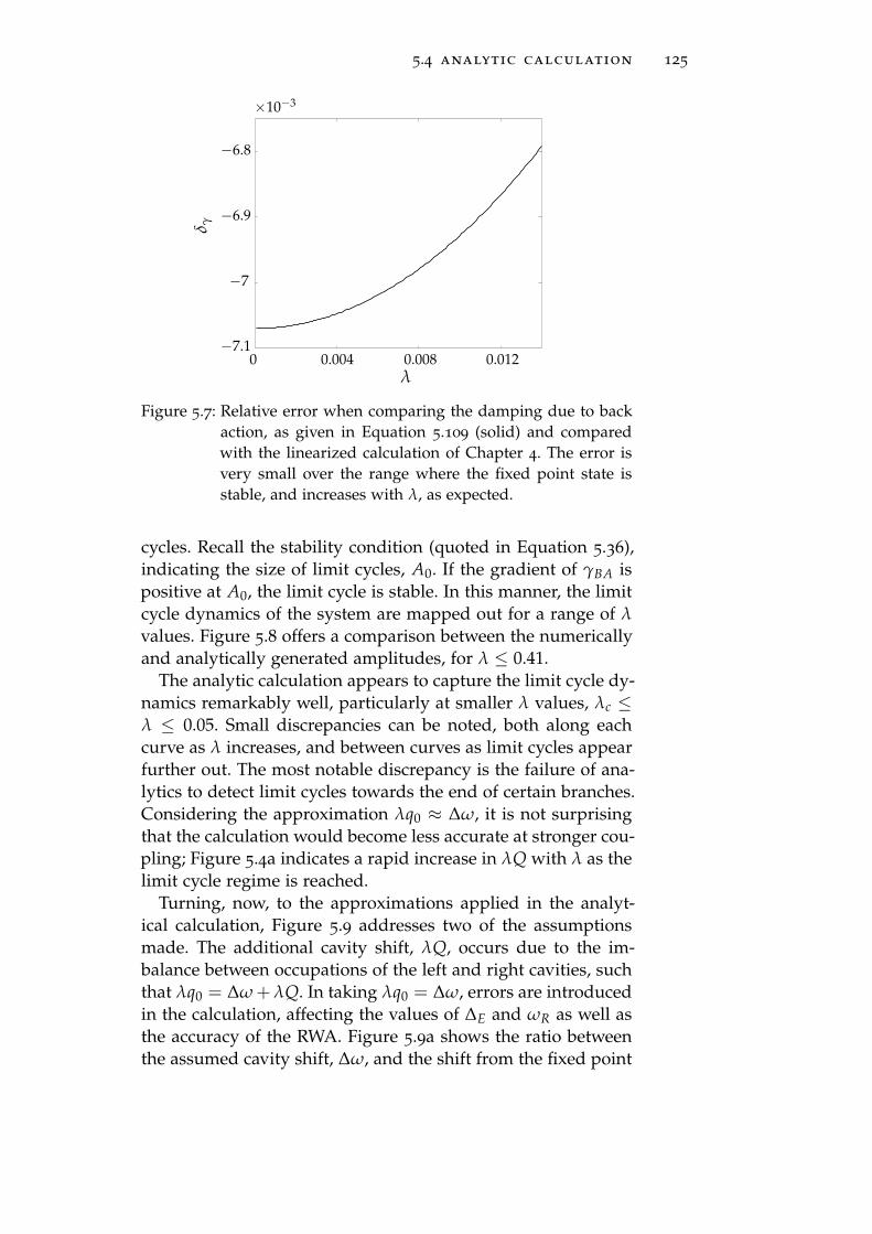
5.4 analytic calculation 125
λ
δ γ
0.0080.004 0.0120−7.1
−6.8
−7
−6.9
×10−3
Figure 5.7: Relative error when comparing the damping due to back
action, as given in Equation 5.109 (solid) and compared
with the linearized calculation of Chapter 4. The error is
very small over the range where the fixed point state is
stable, and increases with λ, as expected.
cycles. Recall the stability condition (quoted in Equation 5.36),
indicating the size of limit cycles, A0. If the gradient of γBA is
positive at A0, the limit cycle is stable. In this manner, the limit
cycle dynamics of the system are mapped out for a range of λ
values. Figure 5.8 offers a comparison between the numerically
and analytically generated amplitudes, for λ ≤ 0.41.
The analytic calculation appears to capture the limit cycle dy-
namics remarkably well, particularly at smaller λ values, λc ≤λ ≤ 0.05. Small discrepancies can be noted, both along each
curve as λ increases, and between curves as limit cycles appear
further out. The most notable discrepancy is the failure of ana-
lytics to detect limit cycles towards the end of certain branches.
Considering the approximation λq0 ≈ ∆ω, it is not surprising
that the calculation would become less accurate at stronger cou-
pling; Figure 5.4a indicates a rapid increase in λQ with λ as the
limit cycle regime is reached.
Turning, now, to the approximations applied in the analyt-
ical calculation, Figure 5.9 addresses two of the assumptions
made. The additional cavity shift, λQ, occurs due to the im-
balance between occupations of the left and right cavities, such
that λq0 = ∆ω + λQ. In taking λq0 = ∆ω, errors are introduced
in the calculation, affecting the values of ∆E and ωR as well as
the accuracy of the RWA. Figure 5.9a shows the ratio between
the assumed cavity shift, ∆ω, and the shift from the fixed point

126 two mode driven dynamics
λ
A0
0.1 0.2 0.3 0.4
80
120
160
0λc
40
Figure 5.8: Analytic calculation of limit cycle sizes (solid lines), us-
ing Equation 5.109 and the analysis outlined in Chapter 2.
This is compared to the numerical data generated in Sec-
tion 5.3 (crosses). As seen in Figure 5.5, the stable cycles
lie along smooth curves separated into different branches.
The two sets of results prove to match closely, with the
main discrepancies arising towards the end of each branch,
where analytics fail to predict limit cycles seen in numer-
ical calculations. The vertical dotted line at λc indicates
where the instability arises and limit cycles emerge.
displacement, λQ (calculated numerically). Qualitatively, there
is a clear increase with λ along each curve, as well as sharp
increases between curves that is consistent with the decreases
in accuracy noted along and between branches in Figure 5.8.
However, quantitatively the λQ values plotted are very high,
compared with ∆ω. In light of such large cavity shifts, the ac-
curacy of the analytic calculation is perplexing.
Also shown, in Figure 5.9b, is the relative error between the
frequency of oscillations in q(t) and the mechanical frequency,
δωm = (ωe f f − ωm)/ωm. For the range plotted, δωm < 0.1,
so that the shift remains small - however there is a noticeable
increase in δωm for the first branch as λ → 0.4, where the an-
alytics begin to fail. These values appear consistent with the
success of the analytic approach.

5.4 analytic calculation 127
(a) (b)λ
λQ
/δω
0.2 0.30.1 0.4
0.2
0.4
0.6
0 0.1 0.2 0.3 0.4
0
0.02
0.04
0.06
δωm
λ
Figure 5.9: Analysis of quantities ignored in calculating γBA: (a) the
ratio between the cavity shift from the fixed point displace-
ment and the , λQ/∆ω, and (b) the relative error in the
shifted mechanical frequency. In (a), the fixed point ap-
pears to cause a significant shift in the cavity frequency,
in comparison to the equilibrium shift. Whilst in (b) the
correction remains small, there is an increase as λ → 0.4
and the discrepancies appear in the analytics.
(a) (b)λ λ
−0.02
0
0.02
0.1 0.2 0.3 0.40
g 1/
∆E
0
0.1
0.2
0.3
ζ
0 0.1 0.2 0.3 0.4
Figure 5.10: Conditions of the RWA: (a) the coupling term, g1/∆E and
(b) ζ = |∆E − nωm|/|∆E + nωm|. In order to apply the
RWA, these two quantities must be far below unity. It is
evident that the coupling is small for the range consid-
ered. The quantity ζ grows significantly with λ; in par-
ticular, there is a rapid increase near λ = 0.4, where the
analytics fail to capture limit cycles on the first branch of
the curve.
The success of the RWA can be understood by re-addressing
the assumptions with the cavity mode separation defined to
include the additional shift:
∆E = 2√
g20 + (∆ω + λQ)2. (5.116)
To that end, the ratio ζ is defined,
ζ =|∆E − nωm||∆E + nωm|
, (5.117)

128 two mode driven dynamics
and examined alongside the coupling term g1/ωm in Figure
5.10. It is immediately apparent that g1/ωm ≪ 1 for the range
of λ in question so that the weak coupling condition of the
RWA is satisfied. It is also required that ζ ≪ 1, in order for the
system to be close to resonance. For λ < 0.3, the ratio ζ remains
below 0.2. This suggests that the system is indeed close to reso-
nance, and the RWA is relatively accurate. For λ > 0.3 the ratio
increases rapidly, and bigger discrepancies occur between the
results in Figure 5.8 - this is where the analytics start to fail at
predicting the presence of certain limit cycles.
5.5 conclusion
In conclusion, this chapter has mapped out the dynamics of the
driven regime for a multimode optomechanical system. A va-
riety of behaviours have been investigated numerically, includ-
ing the emergence of multiple limit cycles and chaos. Whilst
the presence of multiple attractors prohibits a truly systematic
analysis of the system, a fairly detailed picture of the limit cy-
cle dynamics has been obtained for weaker coupling values.
Furthermore, this aspect of the dynamics has been explored an-
alytically. A rotating wave approximation allows an incredibly
accurate prediction of the limit cycle amplitudes in the weak
coupling regime. The success of the calculation seems surpris-
ing, considering the significant contribution to the cavity shift
which is ignored, however closer inspection reveals that the as-
sumptions of the rotating wave approximation are met suffi-
ciently to allow for an accurate calculation.

Appendices
129


AD E TA I L S O F W I G N E R T R A N S F O R M AT I O N
Given a master equation,
ρ = −i[
He f f , ρ]
+ Lmρ + Lcρ, (A.1)
it is possible to perform a transformation which results in a
c-number equation for the system - a semi-classical equation
in terms of complex numbers[50]. The benefit of this is that, in
certain cases, a Fokker-Planck type equation can obtained, from
which Langevin equations of motion can be deduced. For this
particular system, a further approximation will be required in
order to obtain a Fokker-Planck equation[1, 31].
This type of transformation is possible using a number of dif-
ferent representations[1] including the P and Q-representations.
In this instance, the Wigner representation is chosen, as it of-
fers the most simple transformation for evaluating averages
of symmetrically ordered products of creation and annihila-
tion operators. The system is then described in terms of a set
of semi-classical variables whose moments correspond to av-
erages of symmetrically ordered operators (as demonstrated
in Equations 2.25 and 2.26). The Wigner function is defined
in Equation 2.23, and can be thought of as the quantum me-
chanical analogue of the classical probability distribution. The
transformation is performed by first defining the Wigner trans-
formations on individual operators, then deducing the action
on multiple operators.
The Wigner transformations on operators a and a∗ are de-
fined [1]
W(a) = α (A.2)
W(a†) = α∗, (A.3)
where α and α∗ are semi-classical variables which replace the
quantum operators a and a†. The Wigner function of the density
operator W(ρ) is unknown, as ρ cannot be specified, so equa-
tions are written in terms of W(ρ). The Wigner transformation
proceeds by writing Wigner functions for each term in the mas-
ter equation 2.21. Each term consists of products of operators a,
a†, b, b† and ρ. With Wigner functions for each of these opera-
tors defined, a transformation is applied, which allows Wigner
131

132 details of wigner transformation
functions of products of operators, W(AB), to be expressed as
functions of the Wigner functions for the individual operators,
W(A) and W(B):
W(AB) = W(A)e12
(←−∂ α−→∂ α∗−
←−∂ α∗−→∂ α
)
W(B), (A.4)
where←−∂ α denotes a differential acting to the left, and
−→∂ α de-
notes a differential acting to the right.
Equation A.4 can be applied to transform the expanded terms
of Equation 2.21, the term i∆a†aρ transforms as
W(i∆a†aρ) = i∆W(a†a)e12
(←−∂ α−→∂ ∗α−
←−∂ ∗α−→∂ α
)
W(ρ) (A.5)
= i∆
[
W(a†)e12
(←−∂ α−→∂ ∗α−
←−∂ ∗α−→∂ α
)
W(a)
]
×
e12
(←−∂ α−→∂ ∗α−
←−∂ ∗α−→∂ α
)
W(ρ) (A.6)
= i∆(α∗ − 1
2∂α)(α +
1
2∂α∗)W(ρ) (A.7)
= i∆
[
α∗α− 1
2+
1
2(α∗∂α∗ − α∂α)−
1
4∂α∗∂α
]
W(ρ) (A.8)
Treating further terms in the same way as this leads to the final
form of the c-number equation, given in Equation 2.27.
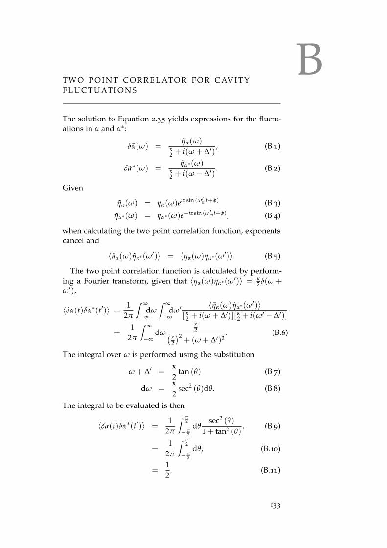
BT W O P O I N T C O R R E L AT O R F O R C AV I T Y
F L U C T U AT I O N S
The solution to Equation 2.35 yields expressions for the fluctu-
ations in α and α∗:
δα(ω) =ηα(ω)
κ2 + i(ω + ∆′)
, (B.1)
δα∗(ω) =ηα∗(ω)
κ2 + i(ω− ∆′)
. (B.2)
Given
ηα(ω) = ηα(ω)eiz sin (ω′mt+φ) (B.3)
ηα∗(ω) = ηα∗(ω)e−iz sin (ω′mt+φ), (B.4)
when calculating the two point correlation function, exponents
cancel and
〈ηα(ω)ηα∗(ω′)〉 = 〈ηα(ω)ηα∗(ω
′)〉. (B.5)
The two point correlation function is calculated by perform-
ing a Fourier transform, given that 〈ηα(ω)ηα∗(ω′)〉 = κ2 δ(ω +
ω′),
〈δα(t)δα∗(t′)〉 =1
2π
∫ ∞
−∞dω
∫ ∞
−∞dω′
〈ηα(ω)ηα∗(ω′)〉[ κ
2 + i(ω + ∆′)][ κ2 + i(ω′ − ∆′)]
=1
2π
∫ ∞
−∞dω
κ2
(
κ2
)2+ (ω + ∆′)2
. (B.6)
The integral over ω is performed using the substitution
ω + ∆′ =κ
2tan (θ) (B.7)
dω =κ
2sec2 (θ)dθ. (B.8)
The integral to be evaluated is then
〈δα(t)δα∗(t′)〉 =1
2π
∫ π2
−π2
dθsec2 (θ)
1 + tan2 (θ), (B.9)
=1
2π
∫ π2
−π2
dθ, (B.10)
=1
2. (B.11)
133

134 two point correlator for cavity fluctuations
With this in mind, the term α∗α − 12 can be evaluated, by
averaging the second order fluctuations:
α∗α− 1
2= 〈α∗〉〈α〉+ 〈α∗〉δα + 〈α〉δα∗ + 〈δα∗δα〉
−1
2(B.12)
= 〈α∗〉〈α〉+ 〈α∗〉δα + 〈α〉δα∗, (B.13)
which gives the expression in Equation 2.46.

CD E TA I L S O F N U M E R I C A L C A L C U L AT I O N
In Chapters 2 and 3 a master equation is written for the system.
The numerical approach involves analysing the dynamics of the
resonator by solving the master equation directly, giving ρ. The
equation takes the form
ρ(t) = Lρ(t), (C.1)
where ρ(t) is the density matrix and L the Liouvillian, a super-
operator. In order to solve this as an eigenvalue equation, it is
written in Liouville space representation [60, 77]; matrices are
transformed to vectors by writing out columns consecutively as
a single column, then L can be written as a matrix, which acts
on the vector ρ in the same way as the super operator on the
matrix ρ. This is denoted in the following way:
|ρ〉〉 = L|ρ〉〉 (C.2)
The matrix L is non-Hermitian, and has a separate set of right
and left eigenvectors:
L|Rn〉〉 = Λn|Rn〉〉 (C.3)
〈〈Ln|L = Λn〈〈Ln|, (C.4)
where in the absence of degeneracy, the eigenvectors can be
assumed to form a complete orthonormal set[60]. A solution
to Equation C.2 can be found, then expanded in terms of the
eigenvalues, Λn:
|ρ(t)〉〉 = eLt|ρ(0)〉〉 (C.5)
= |ρSS〉〉+N−1
∑n=0
〈〈Ln|ρ(0)eΛnt|Rn〉〉, (C.6)
where ρ(0) is an initial density matrix and the matrix L has
N eigenvalues Λn. The eigenvector with zero eigenvalue λ = 0
and right eigenvector, |R0〉〉, is the steady state density operator,
|ρSS〉〉 and normalised to give 〈〈L0| = 〈〈 I|. All further eigen-
values satisfy ℜ[Λn] < 0[78] and describe different timescales
in the evolution of the system. Solutions for ρ(t) can then be
expressed using an eigendecomposition of the matrix L. The
135

136 details of numerical calculation
result is a sum of the steady state density matrix together with
a series of transient terms.
The eigenvector |ρSS〉〉 is found by solving Equation C.2 nu-
merically. In general, in infinite number of states are available
to the cavity and resonator. In order to perform numerical anal-
ysis, however, the spaces of cavity and resonator state must be
truncated to a finite number of states. This produces accurate
results, provided parameters are chosen such that there is a
negligible probability of the cavity(resonator) occupying states
with energies higher than Na(Nb). The matrix L therefore con-
tains(
N2a × N2
b
)2elements. In this thesis, parameters of interest
generally require an order of Nb ∼ 100 resonator states, which
generates matrices too large to deal with. This is tackled by ob-
serving that most of the off diagonal elements are negligible
in size, and can be discarded. The calculation proceeds by con-
sidering only a finite number of off-diagonal elements. Checks
are included in the calculation so that when the matrix is re-
duced, the elements discarded are below a certain value, or the
number included will be increased.

DT R A N S F O R M AT I O N O F H A M I LT O N I A N F R O M
U N C O U P L E D T O C O U P L E D C AV I T Y M O D E S
Here the transformation from equation 3.3 to 3.12 is detailed.
This describes the transformation between operators aL, aR with
frequencies ωL and ωR, and operators a1 and a2 with frequen-
cies ω1 and ω2. A Bogoliubov transformation is applied to the
vector(
aL aR
)T, this takes the form
(
a1
a2
)
=
(
u v
x y
)(
aL
aR
)
. (D.1)
Operators aL and aR represent the left and right modes, with
frequencies ωL and ωR, while the upper and lower branches of
the dispersion curve (Figure 3.1b) are described by operators a1
and a2 with frequencies ω1 and ω2 respectively. Coefficients u,
v, x and y are found by imposing commutation relations to a1
and a2:
[a1(2), a†1(2)] = 1 (D.2)
[a1(2), a1(2)] = 0 (D.3)
[a†1(2), a†
1(2)] = 0 (D.4)
[a1(2), a†2(1)] = 0 (D.5)
Relations between u, v, x, y follow:
u2 + v2 = x2 + y2 = 1 (D.6)
ux + vy = 0 (D.7)
The cavity modes are governed by the Hamiltonian
Hcav = ωLa†LaL + ωRa†
RaR + g(
a†LaR + a†
RaL
)
, (D.8)
so that equations of motion are given by(
aL
aR
)
=
( −iωL − ig
−ig− iωR
)(
aL
aR
)
(D.9)
Differentiating equations D.1 and substituting in equation D.9
gives(
a1
a2
)
= −i
(
uωL + vg ug + vωR
xωL + yg xg + yωR
)(
al
aR
)
.(D.10)
137

138 transformation on cavity modes
Upper and lower branch modes are expected to evolve as
(
a1
a2
)
= −i
(
ω1
ω2
)(
a1
a2
)
. (D.11)
Coefficients are solved for by applying condition D.6:
v =ω1 −ωL
√
g2 + (ω1 −ωL)2(D.12)
u =g
√
g2 + (ω1 −ωL)2(D.13)
x =ω2 −ωR
√
g2 + (ω2 −ωR)2(D.14)
y =g
√
g2 + (ω2 −ωR)2(D.15)
Frequencies ω1,2 are the eigenvectors, ω, of the matrix in D.9
−i
∣
∣
∣
∣
ωL −ω g
g ωR −ω
∣
∣
∣
∣
= 0 (D.16)
(ωL −ω)(ωR −ω)− g2 = 0 (D.17)
ω =ωL + ωR
2±√
(ωL −ωR)2
4+ g2 (D.18)
ω = ω0 ±√
(λq)2 + g2, (D.19)
where the frequencies ω1,2 are then identified as the positive
and negative roots in Equation D.19:
ω1 = ω0 +√
(λq)2 + g2, (D.20)
ω2 = ω0 −√
(λq)2 + g2. (D.21)
The Hamiltonian is then written in terms of the upper and
lower branches:
H = ω1a†1a1 + ω2a†
2a2 +1
2ωm(q
2 + q2)
+Ω(aLeiωdt + a†Leiωdt). (D.22)
The drive term can be written in terms of a1,2,
Hd = Ω(aLeiωdt + a†Le−iωdt) (D.23)
= Ω(Xa†1e−iωdt −Ya†
2e−iωdt + Xa1eiωdt
−Ya2eiωdt), (D.24)

transformation on cavity modes 139
where X and Y are given by
X =y
uy− vx(D.25)
Y =v
uy− vx(D.26)
A unitary transformation eliminates time dependence,
H0 = ωd(a†1a1 + a†
2a2) (D.27)
U = eiH0t/h, (D.28)
giving a drive term
Hd = Ωd
[
X(a1 + a†1)−Y(a2 + a†
2)]
, (D.29)
and an effective Hamiltonian of
He f f = Hint − H0, (D.30)
(D.31)
where Hint = UHU†.


ER O U T H H U RW I T Z S TA B I L I T Y C R I T E R I O N
Consider a system with n degrees of freedom. In a linearized
problem, coupled differential equations can be written for the
fluctuations, in matrix form as follows:
xn
˙xn−1...
x0
= M
xn
xn−1...
x0
, (E.1)
where M describes the time evolution of the vector ~x. If oscilla-
tory solutions are sought in the form ~x(t) = ~x0eΛt, the problem
becomes an eigenvalue equation:
∣
∣
∣
∣
∣
∣
∣
∣
∣
M1,1 −Λ M1,2 · · · M1,n
M2,1 M2,2 −Λ · · · M2,n...
. . .
Mn,1 Mn,n −Λ
∣
∣
∣
∣
∣
∣
∣
∣
∣
xn
xn−1...
x0
= 0, (E.2)
where non trivial solutions are sought by setting detM−Λ =0. The variable Λ is then the solution to a polynomial of root n:
anΛn + an−1Λn−1 + . . . + a1Λ + a0 = 0 (E.3)
There are n roots to the polynomial, which, in general are com-
plex. In order for ~x(t) to be a stable fluctuation, the real part of
each solution, Λ must be negative. Without explicitly solving
for Λ, the stability of solutions can be determined by the Routh
Hurwitz Criterion, which analyses the coefficients a0 through
an. There are two criteria to be met:
1. All coefficients must be real, non zero and have the same
sign.
2. The elements in the first column of the Routh Array must
all have the same sign.
The last condition is based on an object called a Routh array,
which is constructed from combinations of the coefficients as
described in table E.1. The elements in the first two rows are
141

142 routh hurwitz stability criterion
given by alternating coefficients from the polynomial in ques-
tion. Further elements in each row are given by determinants
of two by two matrices formed from adjacent elements in the
array, with the bottom left corner lying directly above the ele-
ment in question. For a polynomial of order n, the Routh array
has n + 1 rows. To clarify, an example is given below:
an an−2 . . .
an−1 an−3 . . .
b1 b2 b3 . . .
c1 c2 c3 . . .... . . .
Table E.1: The Routh array, with elements defined in terms of the co-
efficients of the polynomial in question. Elements of the
left column must be positive in order to satisfy the second
condition.
b1 =
∣
∣
∣
∣
an an−2
an−1 an−3
∣
∣
∣
∣
, (E.4)
=anan−3 − an−2an−1
an−1. (E.5)
e.1 routh array for the static bistability
The Routh array for Equation 4.47 is shown in Table E.2, and
consists of seven rows. With the proviso that elements a6 to a0
are positive (see Section 4.3.1), one requires elements b1 to f1 to
be positive. For element b1 this is possible to show:
b1 =a5a4 − a6a3
a5(E.6)
=κ(
4g2 + 5κ2 + 4κγ + γ2 + 2(∆2L + ∆2
R) + γω2m
)
4κ + γ, (E.7)
which is always positive, since κ and γ are positive. The element
f1 is given by a0, which is positive in the case ηd > 0.
For further elements in the array, however, expressions are
long and cumbersome. It is not possible to deduce their positiv-
ity analytically - however, plots of the elements for the range of
parameters considered are shown in Figure E.1, and are indeed
positive. Whilst this doesn’t prove definitively that the second
condition is always met, it is at least met for this example, in
the range where ∆L, ∆R > 0.
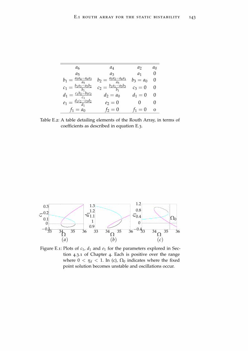
E.1 routh array for the static bistability 143
a6 a4 a2 a0
a5 a3 a1 0
b1 = a5a4−a6a3a5
b2 = a5a2−a6a1a5
b3 = a0 0
c1 = b1a3−a5b2b1
c2 = b1a1−a5b3b1
c3 = 0 0
d1 = c1b2−b5c2c1
d2 = a0 d1 = 0 0
e1 = d1c2−c5d2d1
e2 = 0 0 0
f1 = a0 f2 = 0 f1 = 0 0
Table E.2: A table detailing elements of the Routh Array, in terms of
coefficients as described in equation E.3.
Ω
c 1 d1
Ω Ω
e 1
(a) (b) (c)
Ω0
3433 35 36−0.4
0
0.4
0.8
1.2
3433 35 363433 35 36−0.1
00.1
0.2
0.3
0.91
1.11.21.3
Figure E.1: Plots of c1, d1 and e1 for the parameters explored in Sec-
tion 4.3.1 of Chapter 4. Each is positive over the range
where 0 < ηd < 1. In (c), Ω0 indicates where the fixed
point solution becomes unstable and oscillations occur.


FR O TAT I N G WAV E A P P R O X I M AT I O N F O R
E V E N N
In Chapter 5 the RWA is applied to give expression for the
coefficients c±, which can be solved analytically. The analysis
is presented for the case of odd n (with results presented for
n = 1), but can be generalised for all n. Below the calculation
is explicitly shown for the case where n is even, to show how a
similar result is reached.
Equations 5.75 to 5.78 give the matrix elements for V, for
even n these are
V++ = 2 ∑ν
gν fνux (F.1)
V−− = 2 ∑ν
gν fνvy (F.2)
V+− = ∑ν
gν fν(uy + vx) (F.3)
V−+ = V+−. (F.4)
Substituting equations 5.70 to 5.73 gives
V++ =2g0
∆E(F.5)
V−− = −V++ (F.6)
V+− =−2λq0
∆E. (F.7)
(F.8)
Note that the matrix elements V++ and V−− do not vanish in
this case.
The coefficients then obey the following equations of motion:
ic+ = ∑ν
[
2g0
∆Egν
[
eiνωmt + e−iνωmt]
c+
−2λq0
∆Egν
[
eiνωmt + e−iνωmt]
ei∆E(t−t′)c−
]
(F.9)
ic− = ∑ν
[
− 2λq0
∆Egν
[
eiνωmt + e−iνωmt]
e−i∆E(t−t′)c+
−2g0
∆Egν
[
eiνωmt + e−iνωmt]
c−
]
. (F.10)
145

146 rotating wave approximation for even n
Applying the RWA, only terms with exponents ±|∆E− nωm|are retained, giving
c+ = i ∑ν
2λq0
∆Egnei(∆E−νωm)(t−t′)e−iνωmt′c− (F.11)
c− = i ∑ν
2λq0
∆Egne−i(∆E−νωm)(t−t′)eiνωmt′c+, (F.12)
which are almost identical to Equations 5.94 and 5.95, for the
odd n case, save for a factor of 2λq0/∆E. The remaining analysis
then proceeds by redefining gn as g′n:
g′n =2λq0g
∆EJn
(
2λA
ωm
)
. (F.13)

B I B L I O G R A P H Y
[1] D. F. Walls and G. J. Milburn. Quantum Optics. Springer-
Link: Springer e-Books. Springer, (2008).
[2] M. Planck. Ueber das Gesetz der Energieverteilung im
Normalspectrum. Annalen der Physik, 309:553–563, (1901).
[3] A. Einstein. ber einen die Erzeugung und Verwandlung
des Lichtes betreffenden heuristischen Gesichtspunkt. An-
nalen der Physik, 322:132–148, (1905).
[4] R. Villard. Changes Within Physical Systems And/or Conser-
vation of Energy and Momentum: An Anthology of Current
Thought. Contemporary discourse in the field of physics.
Rosen Publishing Group, (2005).
[5] Japanese Aerospace Exploration Agency. Small Solar
Power Sail Demonstrator ’IKAROS’ Successful Solar Sail
Deployment, June (2010).
[6] P. Lebedew. Untersuchungen ber die Druckkrfte des
Lichtes. Annalen der Physik, 311:433–458, (1901).
[7] V. B. Braginsky, Y. I. Vorontsov, and K. S. Thorne. Quan-
tum Nondemolition Measurements. Science, 209:547–557,
(1980).
[8] P. Meystre, M.O. Scully, and North Atlantic Treaty Orga-
nization. Scientific Affairs Division. Quantum optics, exper-
imental gravity, and measurement theory. NATO advanced
science institutes series: Physics. Plenum Press, (1983).
[9] F. Marquardt and S. M. Girvin. Optomechanics. Physics,
2:40, (2009).
[10] J. Qian, A. A. Clerk, K. Hammerer, and F. Marquardt.
Quantum Signatures of the Optomechanical Instability.
Phys. Rev. Lett., 109:253601, (2012).
[11] W. Marshall, C. Simon, R. Penrose, and D. Bouwmeester.
Towards Quantum Superpositions of a Mirror. Phys. Rev.
Lett., 91:130401, (2003).
147

148 Bibliography
[12] P. D. Nation. Nonclassical mechanical states in an op-
tomechanical micromaser analog. Phys. Rev. A, 88:053828,
(2013).
[13] F. Marquardt, J. P. Chen, A. A. Clerk, and S. M. Girvin.
Quantum Theory of Cavity-Assisted Sideband Cooling of
Mechanical Motion. Phys. Rev. Lett., 99:093902, (2007).
[14] J. D. Teufel, T. Donner, Dale Li, J. W. Harlow, M. S. Allman,
K. Cicak, A. J. Sirois, J. D. Whittaker, K. W. Lehnert, and
R. W. Simmonds. Sideband cooling of micromechanical
motion to the quantum ground state. Nature, 475:359–363,
(2011).
[15] D. A. Rodrigues, J. Imbers, and A. D. Armour. Quantum
Dynamics of a Resonator Driven by a Superconducting
Single-Electron Transistor: A Solid-State Analogue of the
Micromaser. Phys. Rev. Lett., 98:067204, (2007).
[16] A. M. Jayich, J. C. Sankey, B. M. Zwickl, C. Yang, J. D.
Thompson, S. M. Girvin, A. A. Clerk, F. Marquardt, and
J. G. E. Harris. Dispersive optomechanics: a membrane
inside a cavity. New Journal of Physics, 10:095008, (2008).
[17] M. R. Vanner. Selective Linear or Quadratic Optomechan-
ical Coupling via Measurement. Phys. Rev. X, 1:021011,
(2011).
[18] C. Biancofiore, M. Karuza, M. Galassi, R. Natali,
P. Tombesi, G. Di Giuseppe, and D. Vitali. Quantum dy-
namics of an optical cavity coupled to a thin semitranspar-
ent membrane: Effect of membrane absorption. Phys. Rev.
A, 84:033814, (2011).
[19] B. M. Zwickl, W. E. Shanks, A. M. Jayich, C. Yang,
A. C. Bleszynski Jayich, J. D. Thompson, and J. G. E. Har-
ris. High quality mechanical and optical properties of com-
mercial silicon nitride membranes. Applied Physics Letters,
92:103125, (2008).
[20] D. J. Wilson, C. A. Regal, S. B. Papp, and H. J. Kimble. Cav-
ity Optomechanics with Stoichiometric SiN Films. Phys.
Rev. Lett., 103:207204, (2009).
[21] G. D. Cole, I. Wilson-Rae, K. Werbach, M. R. Vanner, and
M. Aspelmeyer. Phonon-tunnelling dissipation in mechan-
ical resonators. Nat Commun, 2:231, (2011).
Bibliography 149
[22] J. D. Thompson, B. M. Zwickl, A. M. Jayich, Florian Mar-
quardt, S. M. Girvin, and J. G. E. Harris. Strong disper-
sive coupling of a high-finesse cavity to a micromechanical
membrane. Nature, 452:72–75, (2008).
[23] E. Buks. Decoherence suppression by cavity optomechani-
cal cooling. Comptes Rendus Physique, 13:454 – 469, (2012).
[24] D. Vitali, S. Gigan, A. Ferreira, H. R. Bohm, P. Tombesi,
A. Guerreiro, V. Vedral, A. Zeilinger, and M. Aspelmeyer.
Optomechanical Entanglement between a Movable Mirror
and a Cavity Field. Phys. Rev. Lett., 98:030405, (2007).
[25] J. C. Sankey, C. Yang, B. M. Zwickl, A. M. Jayich, and
J. G. E. Harris. Strong and tunable nonlinear optomechan-
ical coupling in a low-loss system. Nat Phys, 6:707–712,
(2010).
[26] A. B. Matsko, A. A. Savchenkov, V. S. Ilchenko, D. Sei-
del, and L. Maleki. Optomechanics with Surface-
Acoustic-Wave Whispering-Gallery Modes. Phys. Rev. Lett.,
103:257403, (2009).
[27] K. Srinivasan, H. Miao, M. T. Rakher, M. Davanco, and
V. Aksyuk. Optomechanical Transduction of an Integrated
Silicon Cantilever Probe Using a Microdisk Resonator.
Nano Letters, 11:791–797, (2011).
[28] I. Favero and K. Karrai. Cavity cooling of a nanomechan-
ical resonator by light scattering. New Journal of Physics,
10:095006, (2008).
[29] J. et. al. Aasi. Enhanced sensitivity of the LIGO gravita-
tional wave detector by using squeezed states of light. Na-
ture Photonics, 7:613–619, (2013).
[30] D. A. Rodrigues and A. D. Armour. Amplitude Noise Sup-
pression in Cavity-Driven Oscillations of a Mechanical Res-
onator. Phys. Rev. Lett., 104:053601, (2010).
[31] A. Armour and D. Rodrigues. Quantum dynamics of a
mechanical resonator driven by a cavity. Comptes Rendus
Physique, 13:440 – 453, (2012).
[32] A. Schliesser, O. Arcizet, R. Riviere, G. Anetsberger, and
T. J. Kippenberg. Resolved-sideband cooling and position
measurement of a micromechanical oscillator close to the
Heisenberg uncertainty limit. Nat Phys, 5:509–514, (2009).

150 Bibliography
[33] K. Børkje, A. Nunnenkamp, B. M. Zwickl, C. Yang, J. G. E.
Harris, and S. M. Girvin. Observability of radiation-
pressure shot noise in optomechanical systems. Phys. Rev.
A, 82:013818, (2010).
[34] I. Wilson-Rae, N. Nooshi, J. Dobrindt, T. J. Kippenberg,
and W . Zwerger. Cavity-assisted backaction cooling of
mechanical resonators. New Journal of Physics, 10:095007,
(2008).
[35] C. Genes, D. Vitali, P. Tombesi, S. Gigan, and M. As-
pelmeyer. Ground-state cooling of a micromechanical os-
cillator: Comparing cold damping and cavity-assisted cool-
ing schemes. Phys. Rev. A, 77:033804, (2008).
[36] A. Schliesser, P. Del’Haye, N. Nooshi, K. J. Vahala, and T. J.
Kippenberg. Radiation Pressure Cooling of a Microme-
chanical Oscillator Using Dynamical Backaction. Phys. Rev.
Lett., 97:243905, (2006).
[37] C. Metzger, M. Ludwig, C. Neuenhahn, A. Ortlieb,
I. Favero, K. Karrai, and F. Marquardt. Self-Induced Oscil-
lations in an Optomechanical System Driven by Bolometric
Backaction. Phys. Rev. Lett., 101:133903, (2008).
[38] G. Anetsberger, O. Arcizet, Q. P. Unterreithmeier, R. Riv-
iere, A. Schliesser, E. M. Weig, J. P. Kotthaus, and T. J. Kip-
penberg. Near-field cavity optomechanics with nanome-
chanical oscillators. Nat Phys, 5:909–914, (2009).
[39] G. Heinrich, J. G. E. Harris, and F. Marquardt. Pho-
ton shuttle: Landau-Zener-Stuckelberg dynamics in an op-
tomechanical system. Phys. Rev. A, 81:011801, (2010).
[40] J. Larson and M. Horsdal. Photonic Josephson effect, phase
transitions, and chaos in optomechanical systems. Phys.
Rev. A, 84:021804, (2011).
[41] F. Marquardt, J. G. E. Harris, and S. M. Girvin. Dynami-
cal Multistability Induced by Radiation Pressure in High-
Finesse Micromechanical Optical Cavities. Phys. Rev. Lett.,
96:103901, (2006).
[42] T. Carmon, M. C. Cross, and K. J. Vahala. Chaotic Quiv-
ering of Micron-Scaled On-Chip Resonators Excited by
Centrifugal Optical Pressure. Phys. Rev. Lett., 98:167203,
(2007).

Bibliography 151
[43] P. Rabl. Photon Blockade Effect in Optomechanical Sys-
tems. Phys. Rev. Lett., 107:063601, (2011).
[44] J. D. Teufel, Dale Li, M. S. Allman, K. Cicak, A. J. Sirois,
J. D. Whittaker, and R. W. Simmonds. Circuit cavity
electromechanics in the strong-coupling regime. Nature,
471:204–208, (2011).
[45] A. Nunnenkamp, K. Børkje, J. G. E. Harris, and S. M.
Girvin. Cooling and squeezing via quadratic optomechan-
ical coupling. Phys. Rev. A, 82:021806, (2010).
[46] J. C. Maxwell. A Treatise on Electricity and Magnetism. A
Treatise on Electricity and Magnetism 2 Volume Paperback
Set. Cambridge University Press, (2010).
[47] I. Wilson-Rae. Intrinsic dissipation in nanomechanical res-
onators due to phonon tunneling. Phys. Rev. B, 77:245418,
(2008).
[48] A. Venkatesan, K. J. Lulla, M. J. Patton, A. D. Armour, C. J.
Mellor, and J. R. Owers-Bradley. Dissipation due to tunnel-
ing two-level systems in gold nanomechanical resonators.
Phys. Rev. B, 81:073410, (2010).
[49] M. Aspelmeyer, T. J. Kippenberg, and F. Marquardt. Cavity
Optomechanics. ArXiv 1303.0733, (2013).
[50] C. W. Gardiner. Handbook of stochastic methods. Springer
Series in Synergetics, (1985).
[51] H.J. Groenewold. On the principles of elementary quan-
tum mechanics. Physica, (1946).
[52] S Nasiri. Distribution functions in light of the uncertainty
principle. Iranian Journal of Science and Technology, 29:259,
(2005).
[53] L. You, J. Cooper, and P. Zoller. Quantum-classical corre-
spondences for atomic operators: a positive P representa-
tion approach. J. Opt. Soc. Am. B, 12, (1994).
[54] P. Kinsler and P. D. Drummond. Quantum dynamics of the
parametric oscillator. Phys. Rev. A, 43:6194–6208, (1991).
[55] K.F. Riley, P. Hobson, and S.J. Bence. Mathematical Methods
for Physics and Engineering: A Comprehensive Guide. Cam-
bridge University Press, (2006).

152 Bibliography
[56] J. Larson. Dynamics of the JaynesCummings and Rabi
models: old wine in new bottles. Physica Scripta, 76:146,
(2007).
[57] C. H. Metzger and K. Karrai. Cavity cooling of a mi-
crolever. Nature, 432:1002–1005, (2004).
[58] H.J. Weber and G.B. Arfken. Essential Mathematical Methods
for Physicists. Academic Press, (2004).
[59] A. Nunnenkamp, K. Børkje, and S. M. Girvin. Single-
Photon Optomechanics. Phys. Rev. Lett., 107:063602,
(2011).
[60] K. Blum. Density Matrix Theory and Applications. Springer
Series on Atomic, Optical, and Plasma Physics. Springer,
(2012).
[61] D.K. Bhushan. Matrix And Linear Algebra 2Nd Ed. Prentice-
Hall Of India Pvt. Limited, (2009).
[62] A A Clerk, F Marquardt, and K Jacobs. Back-action evasion
and squeezing of a mechanical resonator using a cavity
detector. New Journal of Physics, 10:095010, (2008).
[63] T. J. Kippenberg and K. J. Vahala. Cavity Optomechan-
ics: Back-Action at the Mesoscale. Science, 321:1172–1176,
(2008).
[64] M. Karuza, M. Galassi, C. Biancofiore, C. Molinelli, R. Na-
tali, P Tombesi, G Di Giuseppe, and D Vitali. Tunable
linear and quadratic optomechanical coupling for a tilted
membrane within an optical cavity: theory and experi-
ment. Journal of Optics, 15, (2013).
[65] K. Thyagarajan and A. Ghatak. Lasers: Fundamentals and
Applications. Graduate Texts in Physics. Springer, (2010).
[66] S. Groblacher, K. Hammerer, M. R. Vanner, and M. As-
pelmeyer. Observation of strong coupling between a mi-
cromechanical resonator and an optical cavity field. Nature,
460:724–727, (2009).
[67] Georg Heinrich. Nanomechanics interacting with light: Dy-
namics of coupled multimode optomechanical systems. PhD the-
sis, Universitt Erlangen-Nrnberg, (2011).

Bibliography 153
[68] G. Heinrich, M. Ludwig, H. Wu, K. Hammerer, and Florian
Marquardt. Dynamics of coupled multimode and hybrid
optomechanical systems. Comptes Rendus Physique, 12:837–
847, (2011).
[69] R. Ghobadi, A. R. Bahrampour, and C. Simon. Quan-
tum optomechanics in the bistable regime. Phys. Rev. A,
84:033846, (2011).
[70] N.K. Sinha. Control Systems. New Age International (P)
Limited, (2008).
[71] U. Weiss. Quantum Dissipative Systems. Series in modern
condensed matter physics. World Scientific, (2012).
[72] E. Verhagen, S. Deleglise, S. Weis, A. Schliesser, and T. J.
Kippenberg. Quantum-coherent coupling of a mechanical
oscillator to an optical cavity mode. Nature, 482:63–67,
(2012).
[73] D. Zill and W. Wright. Differential Equations with Boundary-
Value Problems. Textbooks Available with Cengage You-
book. Cengage Learning, (2012).
[74] H. Wu, G. Heinrich, and F. Marquardt. The effect of Lan-
dauZener dynamics on phonon lasing. New Journal of
Physics, 15:123022, (2013).
[75] D.J. Griffiths. Introduction to quantum mechanics. Pearson
Prentice Hall, (2005).
[76] A. Aspect, W. Barletta, and R. Bonifacio. Coherent and Col-
lective Interactions of Particles and Radiation Beams. IOS Press,
(1997).
[77] T. Harvey. Noise in a dynamical open quantum system: cou-
pling a resonator to an artificial atom. PhD thesis, University
of Nottingham, (2009).
[78] M. Jakob and S. Stenholm. Variational functions in de-
generate open quantum systems. Phys. Rev. A, 69:042105,
(2004).