ab initio nmr chemical shift calculations

4

Ab initio NMR Chemical Shift Calculations for Biomolecular Systems Using Fragment Molecular Orbital Method

A Large-scale Two-phase Flow Simulation on GPU Supercomputer

Evolutive Image/Video Coding with Massively Parallel Computing

ht tp : //www.gsic.titech.ac.jp /TSUBAME_ESJ

01

We have developed two types of fragment molecular orbital (FMO)-based NMR chemical shift calculation methods. They successfully lead to a dramatic reduction of the computational costs by dividing one molecular system into small subsystems and then carrying out calculations on the subsystems in a parallel fashion. Several case studies show that the chemical shift values calculated by our FMO-based methods are in good agreement with those obtained by the standard methods for chemical shift calculation. Our works demonstrate that parallel quantum chemical calculations using a powerful computational resource such as TSUBAME enable us to study a wide range of physical properties of large biomolecules with high accuracy in short time.

Qi Gao*/**　 Satoshi Yokojima**　 Shinichiro Nakamura**　 Minoru Sakurai** Center for Biological Resources and Informatics, Tokyo Institute of Technology**Mitsubishi Chemical Group Science and Technology Research Center, Inc.

In NMR spectroscopy, the chemical shift describes the dependence

of nuclear magnetic energy levels on the electronic environment

in a molecule. In other words, it is a parameter that corresponds to

the difference in resonance frequency between nuclei placed in

different molecular environments. This means that the chemical

shif t is sensitive to various physicochemical factors such as

molecular conformation, configuration, chemical composition, and

surrounding solvent. Thus, observation of chemical shift, usually

combined with those of other NMR parameters (i.e. J-coupling,

relaxation time and NOE), can provide invaluable information

on the three-dimensional structures of molecules, especially in

solution.

However, for large molecules like proteins, it is difficult

to correctly assign their chemical shifts to corresponding 3D

structures only by using experimental approaches. For accurate

structural analysis based on the chemical shift observation,it is

necessary to obtain the information on how the electronic wave

function of a molecule is perturbed by its conformational and

other structural changes. Therefore, theoretical approaches play an

essential role in determining and refining molecular structures in

the framework of NMR spectroscopy. Our work is concerned with

the development of chemical shift calculations for protein on the

basis of quantum mechanics.

Chemical shift in large molecular systems has long been

considered too complicated, or even impossible to be studied by

conventional quantum chemistry calculations. The major problem

concerns the computational cost of calculating chemical shift. For

reliable estimates of chemical shifts, high-level quantum chemical

calculations, based on coupled perturbed methods, are required.

Unfortunately, these methods are computationally very inefficient

and can be applied to small isolated molecules only.

Chemical shift can be evaluated theoretically by solving the

Schrödinger equation in which hamiltonian includes a vector

potential corresponding to the external magnetic field. Here, we

face a new problem. Because we inevitably use finite basis sets,

the calculated chemical shifts depend on the location of gauge

origin of the vector potential. In order to find a numerical solution

for the nuclear magnetic shielding tensor without the gauge

origin dependence, in practice two methods are proposed and

established; the GIAO [4] and CSGT [5].

The GIAO method calculates nuclear magnetic shielding

tensor σαβ as mixed derivatives of the energy E with respect to an

external magnetic field B and nuclear magnetic moment μ. The

gauge origin dependence is eliminated by using field-dependent

atomic orbitals.

The CSGT method calculates the tensor σαβ as the linear

response to an external uniform magnetic field B at the nuclear

In this work, we combine well-established ab initio methods

for chemical shift calculation with the FMO method, which allows

for a rapid calculation for a large molecule by dividing it into small

fragments. In particular, we have used this combined method

to predict the total chemical shifts of ubiqutin, a small (76 resi-

dues) and highly-conserved regulatory protein [1]. Furthermore,

to improve the accuracy of this FMO based NMR chemical shift

calculation method, we develop a method capable of defining an

appropriate fragment size, i.e. a cutoff distance, to better reproduce

the chemical shift values [2,3].

Introduction 1

NMR calculations 2

Ab initio NMR Chemical Shift Calculations for Biomolecular SystemsUsing Fragment Molecular Orbital Method

02

position rN , where J(1)(r) is the induced first-order electronic current

density.

In the CSGT method, the gauge problem is addressed

by redefining the gauge origin R 0 as a parametric function that

depends on the position at which induced current is evaluated.

The chemical shift, δ, is related to the nuclear magnetic-

shielding tensor, σαβ , by a reference standard, σ0 , as

with the absolute isotropic shielding constant,

where superscript x represents monomers (x=I) and dimers (x=IJ).

Here, the RHF calculations of all the monomers and dimers are

performed in the electrostatic potential (ESP) created by the

whole system. The ESP is determined by repeatedly solving the

RHF equation of each monomer until the energy converges self-

consistently. Finally, the RHF equation of every dimer is solved

once including the ESP determined by the previous monomer

FMO calculations. The diagram showing the various steps in the

FMO method is given in Figure 1. Previous FMO studies [6 - 8 ] of

biomolecular systems showed that FMO dimer calculation has

a good compromise between the attained accuracy and the

computational cost incurred.

At the restricted Hartree-Fock (RHF) level of conventional quantum

chemistry theory, the energy E of a molecule is calculated by

solving

the following equation

where F is the Fock matrix, C is a matrix of molecular orbital

coefficients and S is the overlap matrix.

The computational time required to solve the equations

of the Hartree-Fock (HF) theory increases rapidly O（N 3-4）with

system size N; as a result, application of conventional ab initio

methods to biomolecules is too expensive. Therefore, the size of

a typical condensed phase system, such as fully solvated proteins,

necessitates the use of fragment molecular orbital (FMO) method.

In the FMO method, a large molecule is divided into N small

fragments (monomers). Then the total energy is given by

where the sum are over monomer EI and dimer EIJ( pairs of any two

monomers) in the molecule. In the RHF level the contributions to

the total energy due to monomer and dimer can be calculated by

FMO method 3


Figure 1 Computational flow scheme of a typical FMO2 scheme. Every monomer enter the self-consistent field routine, with the electrostatic potential added to the Hamiltonian used to create the Fock matrix F. the calculation keeps running until every monomer converges at the same time.

03

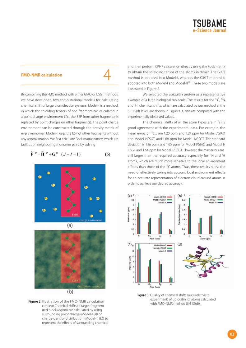
By combining the FMO method with either GIAO or CSGT methods,

we have developed two computational models for calculating

chemical shift of large biomolecular systems. Model-I is a method,

in which the shielding tensors of one fragment are calculated in

a point charge environment ( i.e. the ESP from other fragments is

replaced by point charges on other fragments). The point charge

environment can be constructed through the density matrix of

every monomer. Model-II uses the ESP of other fragments without

any approximation. We first calculate Fock matrix dimers which are

built upon neighboring monomer pairs, by solving

and then perform CPHF calculation directly using the Fock matrix

to obtain the shielding tensor of the atoms in dimer. The GIAO

method is adopted into Model-I, whereas the CSGT method is

adopted into both Model-I and Model-II [1]. These two models are

illustrated in Figure 2.

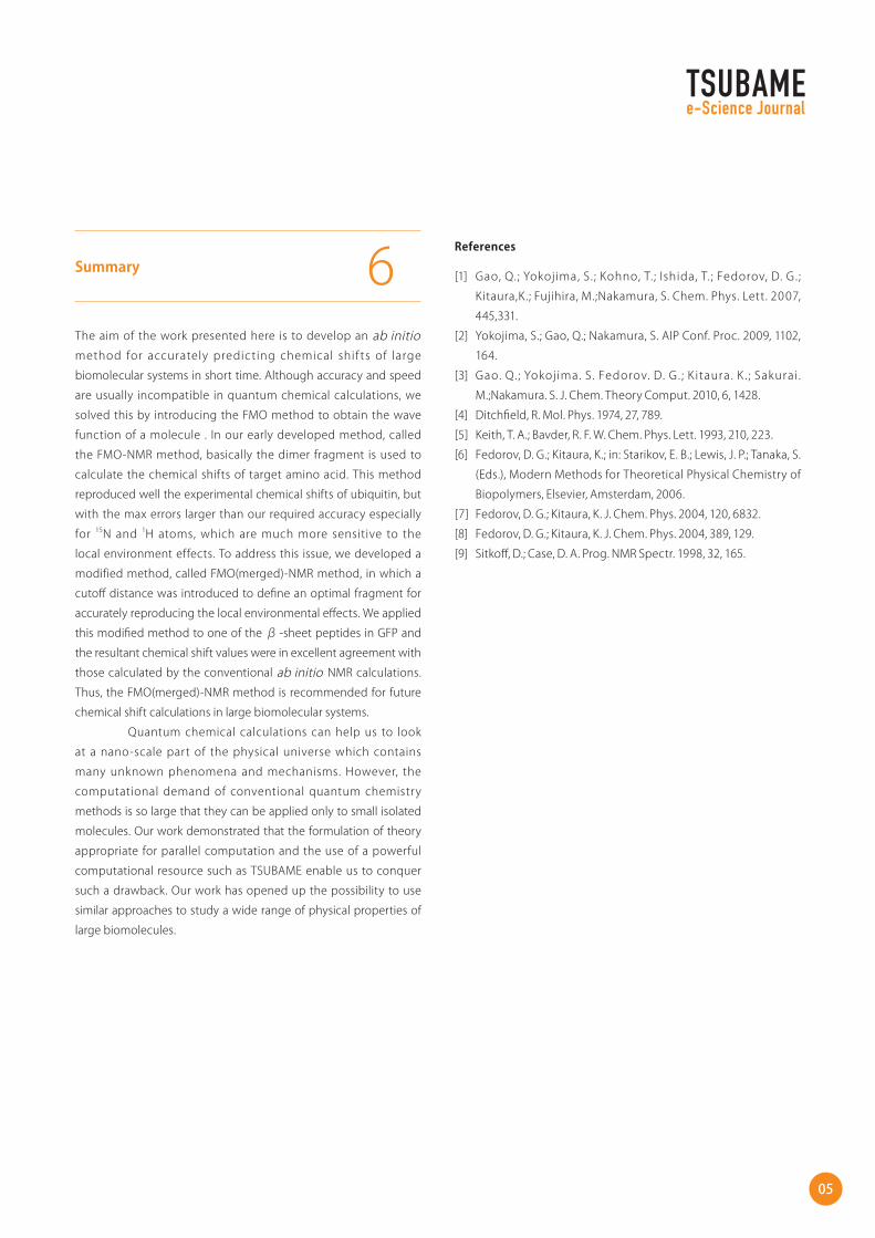
We selected the ubiquitin protein as a representative

example of a large biological molecule. The results for the 13C, 15N

and 1H chemical shifts, which are calculated by our method at the

6-31G(d) level, are shown in Figures 3, and are compared with the

experimentally observed values.

The chemical shifts of all the atom types are in fairly

good agreement with the experimental data. For example, the

mean errors of 13C α are 1.20 ppm and 1.59 ppm for Model I/GIAO

and Model I/CSGT, and 1.68 ppm for Model II/CSGT. The standard

deviation is 1.16 ppm and 1.65 ppm for Model I/GIAO and Model I/

CSGT and 1.64 ppm for Model II/CSGT. However, the max errors are

still larger than the required accuracy especially for 15N and 1H

atoms, which are much more sensitive to the local environment

effects than those of the 13C atoms. Thus, these results stress the

need of effectively taking into account local environment effects

for an accurate representation of electron cloud around atoms in

order to achieve our desired accuracy.

FMO-NMR calculation 4

Figure 3 Quality of chemical shifts (a-c) (relative to experiment) of ubiquitin (d) atoms calculated with FMO-NMR method (6-31G(d)).

Figure 2 Illustration of the FMO-NMR calculation concept.Chemical shifts of target fragment (red block region) are calculated by using surrounding point charge (Model-I (a)) or charge density distribution (Model-II (b)) to represent the effects of surrounding chemical

04

FMO(merged)-NMR calculation 5Although the FMO-NMR method could reproduce well the

corresponding experimental and conventional ab initio calculated

chemical shift data [1], errors of all the atom types were still larger

than the desired level, which is in the range of 1 ppm for heavy

atoms and 0.3 ppm for hydrogen atoms. To obtain an improved

accuracy of calculation results, we proposed a modification to

the FMO-NMR method by introducing the concept of a merged

fragment with a cutoff distance, which defines the optimal merged

fragment size for NMR calculations. We called the method as

FMO(merged)-NMR method.

In the FMO (merged) -NMR method, the point charge

(Model-I) and charge density (Model-II) of every fragment are

first obtained from FMO monomer calculations. Then, a merged

fragment is constructed by assembling all the fragments within a

cutoff distance from the center of target monomer. Subsequently,

the Fock matrix of this merged fragment is evaluated with taking

into account the effect of the surrounding chemical environment.

Finally, the Fock matrix is used to perform the GIAO and CSGT

methods to obtain chemical shift values of the target monomer.

Illustrations of the FMO (merged) -NMR method in Model-I and

Model-II are given in Figure 4.

Aβ-sheet peptide, which is from residues 198 to 229

in green f luorescent protein (GFP), was selected to evaluate

the performance of the FMO(merged)-NMR method. Here, the

cutoff distance was set to 10Å value which is large enough to

accurately reproduce the surrounding effects [9].

In Figure 5 , the errors of chemical shif ts are given

as deviat ions f rom the calculated values obtained by the

conventional ab initio methods. For all the atom types studied,

the errors of the FMO(merged)-NMR calculations are much

smaller than those of the FMO-NMR calculation. For example, in

the case of the chemical shifts of carbon atoms (13Cα and 13Cβ ),

the FMO-NMR calculations give isotropic shielding constants

with a larger maximum error of less than 3 . 8 8 ppm and a

mean error of less than 0 . 8 9 ppm in Model-II [ 2 ] , whereas the

FMO1(merged)-NMR calculations reduces both the maximum

and absolute mean errors of chemical shif ts of carbon atoms,

i.e., to less than 0.15 and 0.05 ppm, respectively. These results

indicate that the FMO(merged)-NMR method provides a much

more accurate local chemical environment description around

the atom of interest than does the FMO-NMR method.


Figure 4 Schematic representation of the FMO (merged)- NMR method. A cutoff distance is used to determine the optimal fragment size (i.e.merged fragment) for accurately calculating the chemical shift of target monomer (orange block region) in both Model-I (a) Model-II (b).

Figure 5 Quality of chemical shifts (a-c) (relative to conventional ab inito calculation results) of a β -sheet (d) atoms in green fluorescent protein calculated with FMO(merged)- NMR method (6-31G(d)).

05

References

[1] Gao, Q.; Yokojima, S. ; Kohno, T. ; Ishida, T. ; Fedorov, D. G. ;

Kitaura,K.; Fujihira, M.;Nakamura, S. Chem. Phys. Lett. 2007,

445,331.

[2] Yokojima, S.; Gao, Q.; Nakamura, S. AIP Conf. Proc. 2009, 1102,

164.

[3] Gao. Q. ; Yokojima. S . Fedorov. D. G . ; K itaura. K . ; Sakurai .

M.;Nakamura. S. J. Chem. Theory Comput. 2010, 6, 1428.

[4] Ditchfield, R. Mol. Phys. 1974, 27, 789.

[5] Keith, T. A.; Bavder, R. F. W. Chem. Phys. Lett. 1993, 210, 223.

[6] Fedorov, D. G.; Kitaura, K.; in: Starikov, E. B.; Lewis, J. P.; Tanaka, S.

(Eds.), Modern Methods for Theoretical Physical Chemistry of

Biopolymers, Elsevier, Amsterdam, 2006.

[7] Fedorov, D. G.; Kitaura, K. J. Chem. Phys. 2004, 120, 6832.

[8] Fedorov, D. G.; Kitaura, K. J. Chem. Phys. 2004, 389, 129.

[9] Sitkoff, D.; Case, D. A. Prog. NMR Spectr. 1998, 32, 165.

The aim of the work presented here is to develop an ab initio

method for accurately predicting chemical shif ts of large

biomolecular systems in short time. Although accuracy and speed

are usually incompatible in quantum chemical calculations, we

solved this by introducing the FMO method to obtain the wave

function of a molecule . In our early developed method, called

the FMO-NMR method, basically the dimer fragment is used to

calculate the chemical shifts of target amino acid. This method

reproduced well the experimental chemical shifts of ubiquitin, but

with the max errors larger than our required accuracy especially

for 15N and 1H atoms, which are much more sensitive to the

local environment effects. To address this issue, we developed a

modified method, called FMO(merged)-NMR method, in which a

cutoff distance was introduced to define an optimal fragment for

accurately reproducing the local environmental effects. We applied

this modified method to one of the β -sheet peptides in GFP and

the resultant chemical shift values were in excellent agreement with

those calculated by the conventional ab initio NMR calculations.

Thus, the FMO(merged)-NMR method is recommended for future

chemical shift calculations in large biomolecular systems.

Quantum chemical calculations can help us to look

at a nano-scale part of the physical universe which contains

many unknown phenomena and mechanisms. However, the

computational demand of conventional quantum chemistry

methods is so large that they can be applied only to small isolated

molecules. Our work demonstrated that the formulation of theory

appropriate for parallel computation and the use of a powerful

computational resource such as TSUBAME enable us to conquer

such a drawback. Our work has opened up the possibility to use

similar approaches to study a wide range of physical properties of

large biomolecules.

Summary 6

06

Two-phase flows such as gas-water mixing are often observed in nature; however, their numerical simulation is one of the most challenging themes in computational fluid dynamics, and it takes a long computational time.A state-of-the-art interface capture method, sparse matrix solver, higher-order advection scheme, and others have been introduced and entirely implemented for GPU computing. It has become possible to carry out large-scale two-phase flow simulations that have never been achieved before. In a violent air-water flow, small bubbles entrained in the water are described clearly and good performance scalability is also shown for multi-GPU computing.

Takayuki Aoki* Kenta Sugihara*** Global Scientific Information and Computing Center, Tokyo Institute of Technology**Graduate School of Engineering, Tokyo Institute of Technology

Recently movie scenes of violent flows mixing air with water

have been produced by computer graphics in Hollywood

film productions. It is notable that they carry out larger-scale

computations with higher-resolution than those of scientific and

engineering works. For two-phase flows, particle methods such as

SPH (smoothed particle hydrodynamics) have been used due to the

simple algorithm and success of astrophysical N-body simulation

in the beginning of GPU computing. Each particle interacts with

all particles within the kernel radius to compute the particle

motion. In three-dimensional simulation, the number of interacting

particles increases, and particle methods have disadvantages from

the viewpoints of numerical accuracy, random memory access,

and amount of computation. In particular, the sparse matrix for

the pressure Poisson equation has a wide bandwidth of non-zero

elements in the semi-implicit time integration and is inefficiently

solved in such memory distributed systems as multi-node clusters

or supercomputers. In addition, there are problems involving non-

physical oscillation at the gas-liquid interface, inaccurate evaluation

of the surface tension, and large numerical viscosity.

In mesh methods such as FDM (finite difference method),

FVM (finite volume method), and FEM (finite element method), the

computation for a mesh point, a cell, or an element requires only

accesses to some neighboring points. Higher-order numerical schemes

are easily applicable to the FDM in structured meshes. In Hollywood

film productions, they have changed the particle methods to mesh

methods to make realistic water scenes. In a mesh method, the gas and

liquid phases are treated as one fluid with different material properties:

density, viscosity, and surface tension. It is necessary to introduce an

interface capturing technique to identify the different properties. The

density changes 1000 times from the gas to the liquid at the interface,

and the profile is expressed with a few meshes.

In this article, we show a large-scale gas-liquid two-

phase simulation by full GPU computing, which has never been

achieved before.

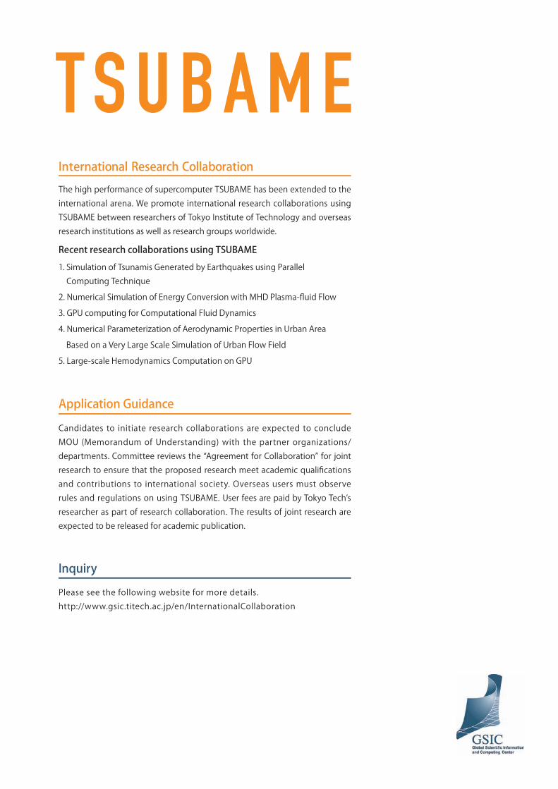
The gas-liquid interface is often described as a surface of a

three-dimensional identical function. The 3-D information

seems to be too much for the 2-D surface information; however,

the method makes it easy to express such topology changes as

splitting and merging of bubbles. The Level-Set function[1] and

the VOF ( volume of fluid) are often used as an identical function.

The former is a signeddistance function from the interface as

shown in Fig.1. In the gas region, it has negative distance, and in

the liquid region, it has positive distance. The interface is expressed

as the zero-level iso-surface of the smooth profile, which is able to

accurately trace the interface.

Introduction and Motivation 1

Gas-liquid interface capturing method 2

A Large-scale Two-phase Flow Simulation on GPU Supercomputer

Figure 1 Iso-surface plots of the Level-Set function**Current position: Japan Atomic Energy Agency

Figure 3 V-cycle of the multi-grid preconditioner.

Figure 4 Bubble shapes depending on Eotvos number (Eo) and Morton number (Mo).

07

3-1 Advection term

For the advection terms of the Navior-Stokes equation and re-

initializing the Hamilton-Jacobi equation, we used the 5th-

order WENO scheme. The high-wavelength filter to preserve

monotonicity contributed the numerical stability. Figure 2

illustrates the stencil access of the 5th WENO scheme. When the on-

chip shared memory was used as a software-managed cache, we

reduced the same access to the off-chip memory (recently the L1

cache is available for this purpose in Fermi-core GPU). For this part,

we have achieved more than 300 GFLOPS on the NVIDIA GTX 280.To confirm the gas-liquid two-phase flow simulation, we compared

it with the experiment of a single bubble rising. In accordance with

the Grace diagram[5], the bubble shape can be spherical, ellipsoidal,

skirted, or dimpled, depending on the dimensionless parameters:

Eotvos number (Eo), Morton number (Mo), and Reynolds number

(Re). For such parameters, the simulation results are in good

agreement with the experimental shapes and rising speeds [6].

by coupling with a V-cycle multi-grid preconditioner shown in

Fig. 3. In the multi-grid process, the ILU method was applied to

the smoother with the Red and Black algorithm.

3-2 Pressure Poisson Solver

It takes a major portion of the computational time to solve the

pressure Poisson equation for two-phase flows. In the case of a

structured mesh, non-zero elements are located regularly in the

sparse matrix; however, their values change 1000 times. We have

developed the BiCGStab method in the Krylov sub-space iteration

in collaboration with MIZUHO Information and Research Institute

as a GPU matrix library. The convergence was drastically improved

The Level-Set method cannot guarantee conservation

of the volumes of the gas and the liquid. We lose small bubbles

and droplets during the computation. On the other hand, the VOF

method conserves the volume and has poor interface shapes when

the curvature radius comes closer to the mesh size.

We introduce the VOF-based THINC[3] WLIC[4] method

to our simulation, in which the anti-diffusion keeps the interface

sharp. We apply the Level-Set method only to evaluate the interface

curvature and the contact angle.

Incompressible Navior-Stokes Solver 3

Single Bubble Rising 4

Figure 2 Stencil of the 5th WENO scheme.

08

It is well known that a milk crown is formed by dropping a droplet

into a glass of shallow milk, and its mechanism and the number

of fingers is still being discussed. The simulation for a liquid with

the same viscosity, surface tension, and impact velocity as the

experiment by Krechetnikov [7] was carried out. Figure 5 exhibits

the typical shape of the milk crown, and it is found that the

simulation reproduces the shapes changing drastically with the

impact velocity.

When dropping a droplet on a dry wall, the edge of the milk

membrane jumps from the wall, which is typically observed in

experiments (see Fig. 6).

To check the simulation for more complex conditions, we studied

the dam-break problem as a typical benchmark in collaboration

with Prof. Hu’s group of the Research Institute for Applied

Mechanics, Kyushu University. By opening the shutter, the dam

water launches onto a dry floor, and the speed of the water edge is

often examined. In our experiment, the floor ahead of the dam was

wet, and a violent wave breaking happened immediately since the

inundating water was decelerated on the wet floor and the wave

behind overtakes it.

In the vessel with the size of 72cm ×13cm × 36cm, water

was filled to a height of 1.8 cm, and a dam that was 15 cm wide and

36 cm high was set initially. We show the time-evolving snapshots

of the simulation results with 576 × 96 × 288 mesh in Fig.8. The last

image is a snapshot of the experiment.

Milk-crown Formation 5 Dam breaking into a wet floor 6

Figure 5 Milk-crown formation

Figure 6 Dispersal of the milk on a dry wall.

Figure 7 Setup of the dam-break experiment

A Large-scale Two-phase Flow Simulationon GPU Supercomputer

09

In our computation, all the components of the two-phase flow

simulation have been implemented on CUDA code. The dependent

variables such as flow velocity, pressure, Level-Set function, and

VOF function were allocated on the on-board GPU memory. The

GPU execution function calls were only requested from the host

CPU, and we removed frequent CPU-GPU communication, which is

a major overhead of GPU computing.

For a large-scale simulation, the computational domain is

decomposed into small domains in which each GPU computation

runs on the on-board video memory. Similar to multi-node CPU

computing, it is required to communicate data among neighbor

domains. The communication between the on-board memories

of different GPUs consists of three steps through a host memory as

shown in Fig. 9.

Multi-GPU computing 7

Figure 9 Data communication between domains for GPU computing.

Figure 8 Simulation and experiment for dam-break problem

The simulation reproduces the wave breaking process well. When

the water impacted with the side wall, it was found that many

small bubbles are entrained into the water [8]. This simulation is

also available for evaluation of the damage caused by a tsunami

impacting on a construction.

Since the communication time between GPUs becomes

a large overhead for large-scale GPU computing, we have

introduced an overlapping technique between communication

and computation[9].

We used 60 nodes of TSUBAME 1.2 with two NVIDIA Tesla

S1070s per node. The performances of the computations with mesh

number 1923, 3843, and 7683 are plotted in Fig. 10. The 4 TFLOPS

performance was achieved in single precision with 108 GPUs [10].

A Large-scale Two-phase Flow Simulationon GPU Supercomputer

10

Figure 10 Performance of two-phase flow computations on multi-GPU computing.

Gas-liquid two-phase flow simulation is one of the challenging CFD

topics, and we executed a simulation on the GPU supercomputer

TSUBAME. A full GPU computation makes it possible to carry

out large-scale computing that has never been done before.

However, there are still problems to be solved, for example, sub-

grid modeling of LES (large eddy simulation) for small bubbles in

high-Reynolds turbulent flows.

Acknowledgements

This research was supported in part by KAKENHI, Grant-in-

Aid for Scientific Research (B) 23360046 from The Ministry of

Education, Culture, Sports, Science and Technology (MEXT), two

CREST projects, "ULP-HPC: Ultra Low-Power, High Performance

Computing via Modeling and Optimization of Next Generation

HPC Technologies" and "Highly Productive, High Performance

Application Frameworks for Post Petascale Computing" from

Japan Science and Technology Agency (JST), and JSPS Global COE

program "Computationism as a Foundation for the Sciences" from

Japan Society for the Promotion of Science (JSPS).

References

[1] M. Sussman, P. Smereka and S. Osher : A Level Set Approach for

Computing Solutions to Incompressible Two-Phase Flow, J.

Comp. Phys., Vol. 114, pp.146-159 (1994)

[2] C．W．Hirt，et al.: SOLA-VOF : A solution algorithm for transient

fluid flow with multiple free boundaries , Los Alamos Scientific

Laboratory，pp.1-32 (1980)

[3] F. Xiao, Y. Honma and T. Kono : A simple algebraic interface

capturing scheme using hyperbolic tangent function, Int. J.

Numer. Method. Fluid., Vol. 48, pp.1023-1040 (2005)

[4] K. Yokoi : Efficient implementation of THINC scheme: A simple

and practical smoothed VOF algorithm, J. Comp. Phys., Vol.

226, pp.1985-2002 (2007)

[5] J .R .Grace : Transac t ions of the Inst i tut ion of Chemical

Engineers, Vol. 51, pp.116-120 (1973)

[6] M. van Sint Annaland, N.G.Deen and J.A.M.Kuipers: Chemical

Engineering Science, Vol. 60, pp.2999-3011 (2005)

[7] R. Krechetnikov and G.M. Homsy : Crown-forming instability

phenomena in the drop splash problem, J. Colloid Interface

Sci., Vol. 331, pp.555-559 (2009)

[8] Takayuki Aoki and Kenta Sugihara: Two-Phase Flow Simulation

on GPU cluster using an MG Preconditioned Sparse Matrix

Solver, SIAM conference on Computational Science and

Engineering 2011, Reno, Nevada (2011)

[9] T.Shimokawabe, T.Aoki, C.Muroi, J.Ishida, K.Kawano, T.Endo,

A.Nukada, N.Maruyama, S.Matsuoka, “An80-foldspeedup,15.0

TFlops full GPU acceleration of non-hydrostatic weather

model ASUCA production code” in Proceedings of the 2010

ACM/IEEE International Conference for High Performance

Computing, Networking, Storage and Analysis, SC’10, IEEE

Computer Society, New Orleans, LA, USA (2010)

[10] Kenta Sugihara and Takayuki Aoki : Multi-GPU acceleration

and s t rong s c a lab i l i t y on a la rge -s c a le h igher- ord er

advection computation, the Japan Society for Computational

Engineering and Science, Transactions of JSCES, Paper

No.20100018 (2010)

Summary 8

11

Evolutionary methods based on genetic programming (GP) enable dynamic algorithm generation, and have been successfully applied to many areas such as plant control, robot control, and stock market prediction. On the other hand, conventional image/video coding methods such as JPEG, MPEG-2, MPEG-4 and AVC/H.264 all use fixed (non-dynamic) algorithms without exception. To relax this limitation, GP has been successfully applied to dynamic generation of pixel prediction algorithm. However, one of the challenges of this approach is its high computational complexity. In this article, we introduce a GP-based image predictor that is specifically evolved for each input image, its good match with parallel computing, and some of speeding-up approaches, which includes the use of massively parallel computation such as TSUBAME2.0 and GPGPU.

Seishi TakamuraNTT Cyber Space Laboratories, NTT Corporation

As for codec applications of the evolutionary method,

Tanaka et al. evolved a “context template” for binary image

coding [2]. Takagi et al. evolved “region segmentation” for video

coding [3]. They both use GA for parameter (context template or

region segmentation) optimization, while their coding algorithms

remain fixed.

2-1 Methodology

GP-based methods enable dynamic algorithm generation, and

have been successfully applied to many areas such as plant control,

robot control, and stock market prediction. We introduce a GP-

based image/video coding approach that is specifically evolved for

each input image. Following is the method of automatic nonlinear

image predictor generation[4,5].

We express the prediction algorithm using the tree

expression. The tree is consisted of leaf nodes (such as immediate

values, surrounding pixel values and the coordinates of the pixel to

be predicted) and non-leaf nodes (such as math functions (e.g., add,

cos), operations (e.g., min, max) and conditional branches). Then,

we initialize the population with randomly generated individuals

(i.e., trees or prediction algorithms) and common predictors such as

MED [6] or GAP[7]. The predictor is evolved through the well-known

GP procedure (i.e., parent selection, children generation (crossover

and mutation) and survival selection). We use the minimal

generation gap method[8] for creating the generations.

For the quantitative metric that measures “how good the

individual (i.e., the predictor) is”, we use the sum of two information

amounts, IT + IR [bits]. IT is the amount of tree information that

represents the predictor's algorithm; it equals the sum of the

information of each node in the tree. IR is the amount of residual

(prediction error) signals' information.

2-2 Prediction Performance

We used four 512x512, 8-bit, gray-scale images (Lena, Baboon,

Airplane, Peppers) for experiment. We tested two evolutionary

predictors, EP4 and EP12. EP4 uses four adjacent pixels. EP12 uses

The Genetic Algorithm (GA) is one approach to optimization

problems; it arranges the “solution parameter” as a one-dimensional

array (a gene). It iterates the emergence of generations via survival

of the fittest to obtain a practical solution parameter. Genetic

Programming (GP)[1], on the other hand, creates a gene tree-structured

to enable “solution method” optimization. Such methods, which are

inspired by organic evolution, are called “evolutionary methods”, and

have been applied to a wide range of fields such as plant control,

stock market prediction, robot control, and analog circuit design.

In image/video coding schemes such as JPEG and AVC/H.264, the

prediction mode, quantization parameter, prediction coefficients,

context grouping thresholds, etc. are adaptively chosen to

optimize the compression performance. So are motion vectors and

prediction modes in video coding. In current image/video coding

schemes, these “coding parameters” are dynamically optimized.

However, the “coding algorithm” itself is never altered within the

scheme. In other words, there has been no way to develop a new

coding scheme other than by human implementation via the trial

and error approach. Therefore, codec complexity cannot exceed

what humans are capable of. Furthermore, it has not been realistic

to develop content-specific (not even image-category-specific)

coding algorithms. Our target then is to develop a scheme that

allows a computer to generate content-specific image/video

coding algorithms. In this overview, we introduce several latest

activities on this evolutionary approach.

Introduction and Motivation 1

Evolution Process Description and Performance 2

Evolutive Image/Video Coding withMassively Parallel Computing

Figure 2 The growth of the tree (from top to downward) with/without tree-size penalty.

12

12 adjacent pixels. For all predictors, the prediction residual was

applied CALIC’s edge-based context separation method [7] to

reduce the entropy. The results are shown in Table 1. In the table,

LS(n) means least-square predictor using surrounding n pixels, LE(n)

means the least-entropy predictor using surrounding n pixels (the

prediction coefficients are optimized off-line to yield the lowest

entropy). It is observed that evolutionary predictor offers better

prediction performance than other methods. Especially, EP4 is even

better than LE(12).

Average predictor size for EP12 was 2062.2 [bits]. As

an example, Peppers’ predictor is shown in Fig. 1. The predictor

includes many mathematical expressions which are beyond

human’s imagination.

Table 1. Residual entropy (overhead inclusive) of the predictors,their increment (“incr.” in percentage) against EP12.Numbers next to the predictors mean the number of reference pixels

Figure 1. Generated predictor (EP12) for Peppers and its conditional branch structure. Ixx are surrounding pixel values. See[5] for more detail of the variables

2-3 Criteria Tweak

In above, we used the criteria which is the sum of tree size and

residual size (i.e., IT + IR). By tweaking the criteria to be minimized,

new features are embodied.

(a) Generation of fast codec

We incorporated encoding time(EncTime) and decoding time

(DecTime) of the individual to the criteria

By tweaking and , we successfly generated fast

encoder or fast decoder while balancing its coding

performance[9].

(b) Tree-size penalty

Since IT is taken into account in the criteria to be minimized,

excessive growth of the tree (so called bloat) is somewhat

suppressed. However, sometimes larger trees have chance to

survive. Suppose there are two predictors (larger and smaller)

of the same coding performance. It is less efficient to enhance

larger tree than to enhance smaller tree, because of the bigger

search space of the larger tree.

Instead of using IT + IR criteria, we applied the weight

(w) to IT [10]. i.e., the new criteria is set to be

The result is shown in Fig. 2. It is clearly seen that applying

penalty yields faster evolution and more compact tree.


13

Figure 3 An image of parallel evolution

Though recent computing processors offer greater and greater

processing capability, the algorithm generation still requires

considerable amount of time. As the predictor grows in size

and complexity, the execution time of the fitness function for

a single predictor increases by several orders of magnitude.

Therefore, acceleration of the evolution computation is strongly

demanded. Evolutive algorithm generation fits quite well with

parallel processing. One example of parallel evolution using

multiple processors/cores is shown in Fig. 3. Each processor/core

does evolution independently, while occasionally observing the

globally-best individual kept in a shared file. Unlike some parallel

processing applications, there is no need to synchronize each

process. Therefore each core works in 100 % load , and addition/

subtraction of processors/cores is quite easy. In addition, there is

also no need to have processors/cores homogeneous.

3-1 Acceleraton with TSUBAME, a parallel computing cluster

The supercomputer TSUBAME of Tokyo Institute of Technology[11]

kindly offered us trial use of it. It has AMD Dual-Core Opteron

2.4GHz, 8CPU, 32GB memory, operating system of SUSE Linux

Enterprise Server 10 (x86_64) Patchlevel 2. Among its more than

10,000 cores, we are allocated about 1,500 cores for the experiment.

In 2010, it has been upgraded to TSUBAME2.0, whose thin nodes

have Intel Xeon X5670 2.93GHz, 12cores/24threads for each,

operating system of SUSE Linux Enterprise Server 11 (x86_64) SP1.

Among its more than 15,000 cores, we used 2,400 cores for the

experiment.

Figs. 4 and 5 show the experimental results. The evolution

acceleration due to the number of the cores is apparent. To

evaluate the effectiveness of parallel processing, the time to reach

certain bit rate (4.407 bits/pel) is shown in Table 2. Its right column

shows the speed-up factor vs. single-core processing. The relation

between number of cores and speed-up factor is depicted in Fig. 6.

Almost linear relation is clearly observed.

3-2 Acceleration with GPU

Advances in GPU hardware in the last several years have

significantly improved their effectiveness for highly parallelizable

programs. Because the fitness function evaluates the predictor

for each pixel in the image, it is an ideal application for the GPU

architecture.

We implemented evolutionary process into GPU using

CUDA platform[12]. We conducted the experiment on a single server

with dual Xeon X5670 2.93 GHz processors (six cores each), four

NVIDIA Tesla C2050 graphics cards (448 CUDA cores each), and 24

GB of memory. Operating System is Ubuntu Server Edition 10.04

(64-bit), and C/C++ compiler is GCC 4.4. For timing individual

predictors, a single CPU core was timed against one Tesla C2050

paired with one CPU core. For predictor evolution, four CPU cores

were timed against four Tesla C2050s, each paired with one CPU

core. The result is shown in Table 3. Throughout various predictor

sizes, GPU achieved ˜140x speed-up consistently.

For image Lena, times to reach 4.493 [bits/pel] were 18.86

hours for CPU and 217 seconds for GPU. In this case GPU achieved 312x

times faster evolution. Its performance transition is shown in Fig.7.

Evolution Acceleration 3

Figure 7 Evolutive predictor’s performance transition for Lena. Red: CPU, green: GPU

Table 2 Time taken to reach 4.407 bits/pel and speed-up factor

14

Figure 4 Compression performance transition with different parallelization degrees

Table 3 Timings and speed-up factors for Lena

Figure 5 Partially magnified version of Fig.ST4 (up to 1 hour)

Figure 6 Speed-up factor according to the number of cores

3-3 Acceleration with class separation

We have seen that the evolved predictor sometimes consists of

conditional branches. For example, the evolved predictor for

image Peppers had the following structure (see Fig. 1):

for each pixel

if (Condition0) Pred0

else if (Condition1) Pred1

else if (Condition2) Pred2

else Pred3

According to these conditions, the predictors (Pred0...3)

are switched pixel-by-pixel. A distribution map of those predictors

is shown in Fig. 8. Apparently, horizontal edges, vertical edges,

highlight areas and the rest are predicted by distinct predictors. It

can be considered that the predictor is evolved so that it adapts

to local image properties (e.g., edge direction and flatness), which

turns out to enhance the prediction performance.

Inspired by the behavior of the evolutive predictor, we

actively classify each pixel according to its local edge direction. We

classified into nine classes: eight classes for eight edge directions

and one class for f lat area (see Figs. 9 and 10 as the example

for the image Peppers). For each class, we evolve the predictor

independently[13]. The time taken to reach these bit rates is shown

in Table 4. It is observed that the speed-up factor for the proposed

method against the conventional method was quite drastic; 25.4-

344.0 (average 180.1x). See Fig. 11 for detailed transition for Peppers.


15

Figure 9 Local edge direction and associated class

Figure 10 classification map (the color corresponds to Fig. 9) for Peppers.

Figure 11 Evolutive predictor’s performance transition. Red: conventional,green: proposed (image = Peppers)

Table 4. Time taken (in minutes) to reach certain bit rate, speed-up factor and predictor size

Discussion and Future Vista 44-1 On ultimate compression

Quite interestingly, Fig. 2 reveals a linear relationship between the

tree size and coding performance. We have observed that every

trial had the same tendency. Therefore it is conjectured that

where k = –50...–35 (the slope in Fig. 2). For typical lossless

compression, rate = 4̃ [bits/pel] (about half of original size).

Since IT ≥ 0 and IR ≥ 0, ultimate compression rate is

attained when IR = 0 (no residue; i.e., the predictor itself contains

image information). Then we have ultimate rate as

This rate ( about 1 % of original size) sounds too low

for lossless coding. It should be noted that the coding rate is

bounded by the amount of the noise in an image, since the noise

is incompressible by nature. However, it is still conjectured that the

ultimate compression rate is close to the noise amount (then the

prediction residual becomes the white noise completely). Another

thing which should be noted is, the evolution speed exponentially

slows down according to the value of IT. So currently it is not

expectable to reach such an ultimate point.

Figure 8 Predictor distribution map for Peppers. Each color (white, blue, green and black) corresponds to a distinct predictor

16

Figure 12 Simple models and associated images

4-2 Reverse-engineering of Image

Further extrapolation of above discussion bethinks us that ultimate

predictor is an indication of the model that is hidden behind the

image data. Following is the minimum toy experiment to see if GP

is powerful enough to reveal such an image model. Three images

were generated from simple model (see Fig.12).

Then, only the image (not the model) was fed into the

evolutive predictor generator. The outcomes were:

respectively. They are all mathematically equivalent to the given

model. In other words, reverse-engineering of the image would be

attained using evolutive coding.

4-3 Self-compressing archive

One of the applications of evolutive coding is its combination with

image/video archive. Making use of excessive computational power

from e.g., the cloud, the archive updates its coding algorithm day

by day, and the size continuously shrinks to yield a space to archive

other images (Fig. 13).

4-4 Category-specific coder

Until here, image-specific algorithm generation has been discussed.

It would be nice if a certain algorithm performs reasonably well for

an image of certain pre-defined category.

We prepared three categories (clouds, city lights and

nature) [14]. Each category contains ten 128 x 128 gray scale images.

The anchor scheme was generated which offers the lowest average

coding rate for all 30 images. Similarly, the evolutionary process

was conducted for each category, and for each image respectively.

Table 5 shows the simulation results. Image-specific

coder (“for image”) is the best as expected. However, category-

specific coder (“for category”) offers only slight performance

loss (˜0.1% ).

4-5 Application to lossy coding

Evolutive image/video coding can be applied not only to lossless

coding but also to lossy coding. By generating content-specific

nonlinear image restoration filter using GP, about 0.9% coding rate

reduction against HEVC, state-of-the-art coding technology under

development, is achieved [15].

Table 5. Bit rates and increase against the anchor (in parentheses)

Figure 13 An image of self-compressing archive


17

In this article, evolutive image/video coding was introduced

regarding its concept, characteristics, potential and future vista.

In particular, its fitness to the parallel processing system such

as TSUBAME/TSUBAME2.0 would surely extend its feasibility.

Therefore the advance of such a high-performance computing

platform is tightly connected to the advance of evolutive image/

video coding.

References

[1] J. Koza, “Genetic Programming II, Automatic Discovery of

Reusable Programs,” The MIT Press, (1998)

[2] M. Tanaka, H. Sakanashi, M. Mizoguchi, T. Higuchi, “Bi-level

image coding for digital printing using genetic algorithm,”

Electronics and Communications in Japan part III: Fundamental

Electronic Science, vol. 84, no. 9, pp. 1-10, (Apr. 2001)

[3] K. Takagi, A. Koike, S. Matsumoto and H. Yamamoto, “Motion

Picture Coding Based on Region Segmentation Using Genetic

Algorithm,” Systems and Computers in Japan, vol. 33, no. 5, pp.

41-50, (Mar. 2002)

[4] S. Takamura, M. Matsumura and Y. Yashima, “Automatic Pixel

Predictor Construction Using an Evolutionary Method,” Proc.

PCS2009, pp. 1-4, (May 2009)

[5] S. Takamura, M. Matsumura and Y. Yashima, “A Study on an

Evolutionary Pixel Predictor and Its Properties,” Proc. ICIP2009,

(Nov. 2009)

[6] “Lossless and Near-Lossless Compression of Continuous Tone

Still Images,” ISO/IEC 14495-1, (2000)

[7] X. Wu and N. Memon, “Context-Based, Adaptive, Lossless

Image Coding,” IEEE Trans. Commun. vol. 45, no. 4, pp. 437-

444, (Apr. 1997)

[8] H. Satoh, M. Yamamura and S. Kobayashi, “Minimal Generation

Gap Model for GAs Consider ing both E xplorat ion and

Exploitation,” Proc. 4th Int. Conf. Soft Computing, pp. 494-497,

(Oct. 1996)

[9] M. Matsumura, S. Takamura and H. Jozawa, “Evolutive Image

Coding Based on Automatic Optimization for Coding Tools

Combination,” Proc. IWAIT2010, (Jan. 2010)

[10] S . Tak amura , “Evo lut ive V ide o Co ding ~From Gener ic

Algorithm towards Content-Specific Algorithm~,” PCS2010

tutorial talk (T1), (Dec. 2010)

[11] http://www.gsic.titech.ac.jp/en

[12] M. McCawley, S. Takamura and H. Jozawa, “GPU-Assisted

Evolutive Image Predictor Generation,” IEICE Tech. Rep., vol.

110, no. 275, IE2010-88, pp. 25-28, (Nov. 2010)

[13] S. Takamura, M. Matsumura and H. Jozawa, “Accelerating Pixel

Predictor Evolution Using Edge-Based Class Separation,” Proc.

PCS2010, P1-22, pp. 106-109, (Dec. 2010)

[14] M. Matsumura, S. Takamura and H. Jozawa, “Generating

Subject Oriented Codec by Evolutionary Approach,” Proc.

PCS2010, P3-13, pp. 374-377, (Dec. 2010)

[15] S. Takamura and H. Jozawa, “A Basic Study on Automatic

Construction of Nonlinear Image Denoising Filter”, Proc.

PCSJ2011, (Oct. 2011) [to appear]

Summary 5

● TSUBAME e-Science Journal No.4Published 10/31/2011 by GSIC, Tokyo Institute of Technology ©ISSN 2185-6028Design & Layout: Kick and PunchEditor: TSUBAME e-Science Journal - Editorial room Takayuki AOKI, Thirapong PIPATPONGSA, Toshio WATANABE, Atsushi SASAKI, Eri NakagawaAddress: 2-12-1-E2-1 O-okayama, Meguro-ku, Tokyo 152-8550Tel: +81-3-5734-2087　Fax: +81-3-5734-3198 E-mail: [email protected]: http://www.gsic.titech.ac.jp/

International Research Collaboration

Application Guidance

Inquiry

Please see the following website for more details.http://www.gsic.titech.ac.jp/en/InternationalCollaboration

The high performance of supercomputer TSUBAME has been extended to the international arena. We promote international research collaborations using TSUBAME between researchers of Tokyo Institute of Technology and overseas research institutions as well as research groups worldwide.

Recent research collaborations using TSUBAME

1. Simulation of Tsunamis Generated by Earthquakes using Parallel　Computing Technique

2. Numerical Simulation of Energy Conversion with MHD Plasma-fluid Flow

3. GPU computing for Computational Fluid Dynamics

4. Numerical Parameterization of Aerodynamic Properties in Urban Area

Based on a Very Large Scale Simulation of Urban Flow Field

5. Large-scale Hemodynamics Computation on GPU

Candidates to initiate research collaborations are expected to conclude MOU (Memorandum of Understanding) with the partner organizations/departments. Committee reviews the “Agreement for Collaboration” for joint research to ensure that the proposed research meet academic qualifications and contributions to international society. Overseas users must observe rules and regulations on using TSUBAME. User fees are paid by Tokyo Tech’s researcher as part of research collaboration. The results of joint research are expected to be released for academic publication.

ab initio nmr chemical shift calculations

Documents