ab initio description of second-harmonic generation from crystal … · the second-harmonic...
TRANSCRIPT

Thèse présentée pour obtenir le grade de
Docteur de l’École polytechnique
Spécialité : Physique
par
Nicolas TANCOGNE-DEJEAN
Ab initio description of second-harmonic generation fromcrystal surfaces
Thèse soutenue publiquement le 21 septembre 2015 devant le jury composé de :
Prof. Stefano OSSICINI RapporteurDr. Christophe DELERUE Rapporteur
Prof. Benoît BOULANGER ExaminateurDr. Phuong Mai DINH Examinateur
Prof. Luca PERFETTI ExaminateurDr. Christian BROUDER ExaminateurDr. Valérie VÉNIARD Directrice de thèse


We can only see a short distance ahead, but we can see plenty there that needs to be done.
Alan Turing


Contents
Preface iii
Abbreviations and notations vii
I Background 1
1 Introduction 3
1.1 Historical background . . . . . . . . . . . . . . . . . . . . . . . . . . . . . . . . . . . . . 3
1.2 Second-harmonic generation . . . . . . . . . . . . . . . . . . . . . . . . . . . . . . . . . 4
1.3 Microscopic-macroscopic connection . . . . . . . . . . . . . . . . . . . . . . . . . . . . . 7
1.4 Longitudinal-transverse and optical limit . . . . . . . . . . . . . . . . . . . . . . . . . . 11
1.5 Present work . . . . . . . . . . . . . . . . . . . . . . . . . . . . . . . . . . . . . . . . . . . 16
2 Second-harmonic generation in reflection 19
2.1 Second-order polarization induced by incident light . . . . . . . . . . . . . . . . . . . . 21
2.2 Harmonic field inside the material . . . . . . . . . . . . . . . . . . . . . . . . . . . . . . 22
2.3 Reflected harmonic light from a surface . . . . . . . . . . . . . . . . . . . . . . . . . . . 24
2.4 Bulk contribution . . . . . . . . . . . . . . . . . . . . . . . . . . . . . . . . . . . . . . . . 26
3 (Time-Dependent) Density-Functional Theory in a nutshell 29
3.1 Time-dependent perturbation theory . . . . . . . . . . . . . . . . . . . . . . . . . . . . . 29
3.2 Density-Functional Theory (DFT) . . . . . . . . . . . . . . . . . . . . . . . . . . . . . . . 32
3.3 Time-Dependent Density-Functional Theory (TDDFT) . . . . . . . . . . . . . . . . . . . 36
3.4 Perturbation theory and TDDFT . . . . . . . . . . . . . . . . . . . . . . . . . . . . . . . 38
3.5 TDDFT in practice . . . . . . . . . . . . . . . . . . . . . . . . . . . . . . . . . . . . . . . . 42
4 Silicon and its (001) surface 47
4.1 Silicon . . . . . . . . . . . . . . . . . . . . . . . . . . . . . . . . . . . . . . . . . . . . . . 47
4.2 The role of silicon surfaces in novel applications . . . . . . . . . . . . . . . . . . . . . . 48
4.3 The (001) surface of silicon . . . . . . . . . . . . . . . . . . . . . . . . . . . . . . . . . . . 49
4.4 Geometries and reconstructions . . . . . . . . . . . . . . . . . . . . . . . . . . . . . . . . 50
i
Contents
II Microscopic theory of second-harmonic generation from crystal surfaces 55
5 Microscopic theory of surface second-harmonic generation 57
5.1 Extracting the surface second-harmonic generation spectra . . . . . . . . . . . . . . . . 58
5.2 Discussions . . . . . . . . . . . . . . . . . . . . . . . . . . . . . . . . . . . . . . . . . . . 69
6 Effects of nonlocal operators on surface second-harmonic generation 79
6.1 Nonlocal operators and perturbation theory . . . . . . . . . . . . . . . . . . . . . . . . . 80
6.2 Numerical results . . . . . . . . . . . . . . . . . . . . . . . . . . . . . . . . . . . . . . . . 86
III Local-field effects in surface optical properties 91
7 Ab initio macroscopic linear and second-order optical properties of crystal surfaces:
From the slab to the single surface 93
7.1 Macroscopic dielectric tensor of crystal surfaces . . . . . . . . . . . . . . . . . . . . . . 94
7.2 Optical limit for the surface macroscopic dielectric function . . . . . . . . . . . . . . . . 96
7.3 Calculation of ǫS,LLM in TDDFT . . . . . . . . . . . . . . . . . . . . . . . . . . . . . . . . . 98
7.4 Macroscopic second-order tensor of crystal surfaces . . . . . . . . . . . . . . . . . . . . 99
7.5 Properties of the surface macroscopic quantities . . . . . . . . . . . . . . . . . . . . . . 106
8 Local-field effects for linear optical properties of thin-films and surfaces 109
8.1 Local-field effects and super-cells . . . . . . . . . . . . . . . . . . . . . . . . . . . . . . . 110
8.2 Mixed-space approach . . . . . . . . . . . . . . . . . . . . . . . . . . . . . . . . . . . . . 113
8.3 Selected-G approach . . . . . . . . . . . . . . . . . . . . . . . . . . . . . . . . . . . . . . 116
8.4 Discussion . . . . . . . . . . . . . . . . . . . . . . . . . . . . . . . . . . . . . . . . . . . . 121
IV Application to Silicon Surfaces 127
9 Local-field effects on second-harmonic generation from surfaces 129
9.1 Local-Field Effects on the clean Si(001) SHG spectra . . . . . . . . . . . . . . . . . . . . 130
9.2 Hydrogenated surfaces and local-field effects . . . . . . . . . . . . . . . . . . . . . . . . 132
9.3 Comparison with experimental results . . . . . . . . . . . . . . . . . . . . . . . . . . . . 134
10 Excitonic effects on second-harmonic generation from silicon surfaces 141
10.1 The α-kernel as a post-processing . . . . . . . . . . . . . . . . . . . . . . . . . . . . . . . 142
10.2 Excitonic effects on the surface second-harmonic generation . . . . . . . . . . . . . . . 147
ii

Contents
Concluding remarks 151
V Appendices 153
A Fourier transforms 155
B Maxwell’s equations 159
C Second-harmonic reflection coefficients for some symmetries 163
D Matrix elements of V in a plane-waves basis 167
E Divergence-free expression of χSρρρ 169
F Macroscopic surface response functions 175
G Analytical expression of vG1,G2(q) 177
H Mixed-space equations for SHG 179
I Optical properties of single surfaces 181
List of publications 186
List of codes 188
Bibliography 191
iii


Preface
The field of nonlinear spectroscopy has matured rapidly but still has much potential for furtherexploration and exploitation. The applications in chemistry, biology, medicine, materialstechnology, and especially in the field of communications and information processing arenumerous. Alfred Nobel would have enjoyed this interaction of physics and technology.
Nicolaas Bloembergen, Nobel Lecture, 1981
Only one year after the invention of the laser in 1960, researchers showed that laser light could beconverted from one color to another. Using a red ruby laser light and a quartz crystal, Frankel andcoworkers have demonstrated the possibility to create an ultraviolet radiation from red light. Thiswas the first demonstration of a nonlinear optical phenomenon.More than 50 years after the first experimental observation of second-harmonic generation, the theo-retical description of second-harmonic generation is still under debate, whereas it is well understoodfrom an experimental point of view. This is the gap that this thesis aims to fill.More precisely, the goal of this work is to improve the theoretical description and understanding ofthe generation of second-harmonic from the surfaces of crystalline semiconductors.When applying an external electric field to a dielectric material, electric dipoles are created at a mi-croscopic level. These dipoles are responsible for the apparition, inside the material, of an inducedfield. The fluctuations of the electric field at a microscopic level, the density fluctuations or any kindof microscopic inhomogeneities must be taken into account when describing the optical propertiesof a system. These effects are often referred as “local-field effects”.These local-field effects have been widely studied in the past and in particular their effects on theoptical properties of bulk materials are now well established. In the case of surfaces, the theoreticaldescription and the numerical simulations are more intricate than for bulk materials. The abruptchange in the electronic density leads to a huge variation of the electric field at the interface withvacuum. As a result, strong effects of the local-field are expected, in particular in the direction per-pendicular to the plane of the surface.The goal of this thesis is to quantify how important these effects are for the linear and second-orderoptical properties of surfaces.This thesis is organised in four parts. The Part I focuses on the theoretical background, necessary tounderstand the development reported in this thesis.Part II presents the first theoretical results of this thesis, improving the microscopic description ofsecond-harmonic generation at crystal surfaces. A macroscopic theory of second-harmonic genera-
v

Contents
tion from crystal surfaces is developed in Part III, in order to account for local-field effects.The last part of this thesis, Part IV, is dedicated to the application of the theory developed to siliconsurfaces. The numerical simulations have been focused on the Si(001) surface, and the macroscopicformalism developed during this thesis has been applied to three surface reconstructions, namely theclean Si(001)2×1, the monohydride Si(001)2×1:H and the dihydride Si(001)1×1:2H surfaces. Compar-ison with available experimental results is also reported.
vi

Abbreviations
AFM Atomic Force MicroscopeBZ Brillouin zoneBSE Bethe-Salpeter equation(TD)DFT (Time-Dependent) Density-Functional TheoryEFISH Electric Field Induced Second-HarmonicHEG Homogeneous Electron GasHK Hohenberg-KohnIPA Independent-Particle ApproximationKS Kohn-ShamLDA Local-Density ApproximationLF Local-fieldsLRC Long-Range ContributionRA Reflectance AnisotropyRPA Random Phase ApproximationSHG Second-Harmonic GenerationTD Time DependentXC Exchange-Correlation
vii


Notations
General
r A point in 3-D space, (x, y, z)t An instant in timeω A frequency (time Fourier transform)k A vector in reciprocal spaceq A vector inside the first Brillouin zoneG A reciprocal lattice vector, also referred as G-vectorf [n] A functional f of the function n
(TD)-DFT and response functions
Etot Ground-state total energyn0(r) Ground-state electronic densityn(r, t) TD electronic densityj(r, t) TD electronic currentΨ Interacting many-body wave-functionφi Single-particle or Kohn-Sham wave-functionχ(1)0 , χ(0)
ρρ Independent-particle density-density response functionχ(1), χ(1)
ρρ Fully interacting density-density response functionχ(2)0 , χ(0)
ρρρ Independent-particle density-density-density response functionχ(2), χ(2)
ρρρ Fully interacting density-density-density response function
Varia
η Positive infinitesimalc Speed of light in the vacuumǫ0 Vacuum permittivity↔1 Unit dyadic
If not stated differently, atomic units are used throughout this thesis.
ix


Part I
Background
1


Chapter 1. Introduction
et al. discovered that applying a dc-electric field to a nonlinear medium was changing the intensityof the second-harmonic generation [5], a process which is now referred as the Electric Field InducedSecond-Harmonic Generation (EFISH). Numerous other nonlinear optical effects have also been dis-covered since 1961 and the discovery of the second-harmonic generation; and nowadays nonlinearoptics is used in many fields of the physics, biology or chemistry but also in neurosciences, in surgery,in data transmission and more recently for producing x-ray laser radiations.
1.2 Second-harmonic generation
In the case of a weak excitation, of frequency ω, the electric polarization P is related to the electricfield E by the relation
Pi(ω) =∑
j
χ(1)ij (ω)Ej(ω), (1.1)
where Pi and Ej are Cartesian components of P and E with i, j ∈ x, y, z.This relation defines the linear dielectric susceptibility χ(1). This regime corresponds to the linearoptics, where the response is proportional to the perturbing electric field. The tensor χ(1) describesthe absorption of light, the reflection at surfaces as well as the loss functions.When the perturbing electric field is more intense, nonlinear effects are no more negligible and wemust account for them.It is possible to generalize the expression Eq. (1.1) (where we have omitted position and frequencyarguments for sake of simplicity)
Pi =∑
j
χ(1)ij Ej +
∑
jk
χ(2)ijkEjEk +
∑
jkl
χ(3)ijklEjEkEl + . . . (1.2)
where χ(2)ijk is a third rank tensor (meaning a 3 indices tensor and so 27 components), which charac-
terizes the second-order nonlinear susceptibility. Due to the symmetric role of the electric fields, thistensor follows the permutation rule χ(2)
ijk = χ(2)ikj .
If we consider the incident fields as being the superposition of two fields oscillating respectively atfrequencies ω1 and ω2, it is possible to obtain many phenomena, summarized in Tab. 1.1.The χ(3)
ijkl tensor describes new phenomena such as the four-waves mixing or the Kerr effect. If the
Second-order process Definition
Frequency doubling χ(2)(−2ω1, ω1, ω1)
Optical rectification 2χ(2)(0, ω1,−ω1)
Sum frequency 2χ(2)(−ω1 − ω2, ω1, ω2)
Frequency difference 2χ(2)(−ω1 + ω2, ω1, ω2)
Tab. 1.1: List of different effects that can occur when two beams oscillating respectively at frequenciesω1 and ω2 propagate in a medium which exhibits a non-zero second-order nonlinear susceptibility. Inthis table, we use the convention where the emitted signal is denoted with a minus sign. Neverthelessthis convention is not used in this thesis.
perturbation is not so intense, we can expect the expansion in power of the electric field Eq. (1.2) to
4

1.2 Second-harmonic generation
converge, and thus to have |χ(2)ijk| ≫ |χ(3)
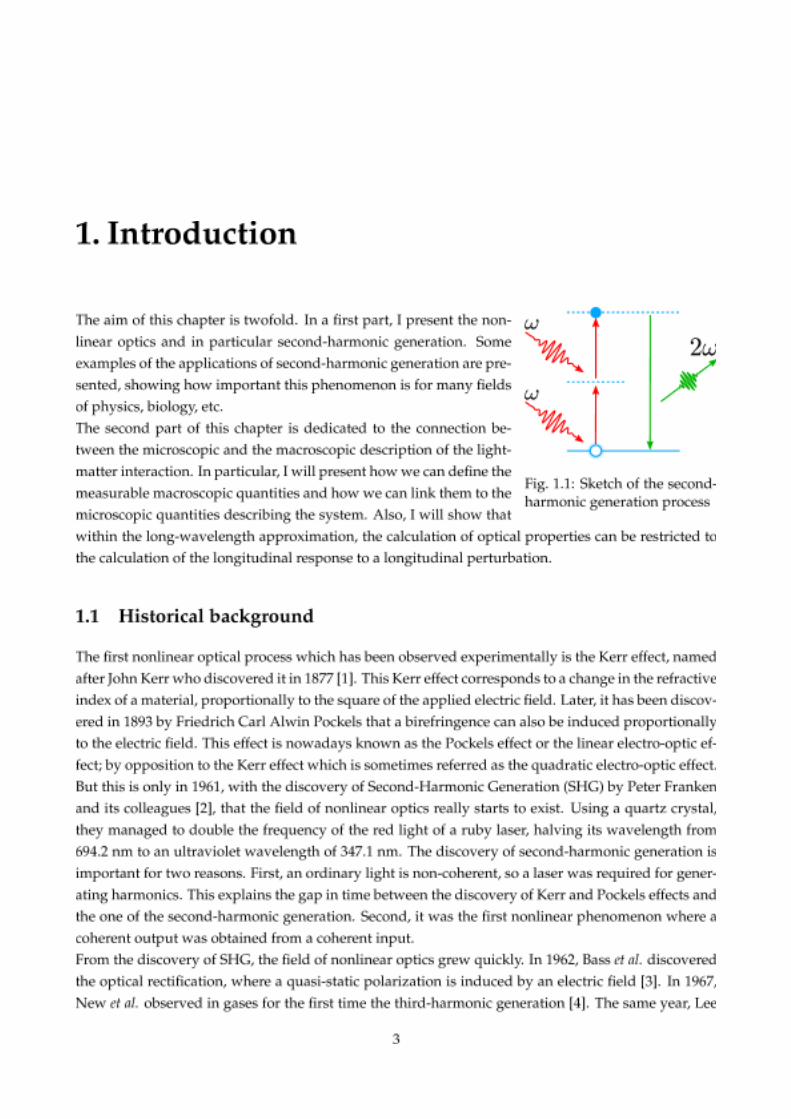
ijkl|. This is not the case for strong laser-fields, e.g., the High-Harmonic Generation (HHG), where a lot of harmonics are obtained with a similar intensity [6]. Inthis thesis, the perturbing laser-field is considered to be weak enough that the expansion Eq. (1.2)converges.As suggested by the title of this thesis, among all possible nonlinear phenomena, only the second-order nonlinear process where ω1 = ω2 = ω, and known as the second-harmonic generation, willbe considered. The second-harmonic generation process can be explained in a very simple versionby the sketch presented in Fig. 1.1. In this picture, two virtual states are involved, i.e., they do notcorrespond to the energy levels of the system. The sketch in Fig. 1.1 describes the absorption of twophoton at the frequency ω and the relaxation to the ground-state by the emission of a photon, whosefrequency is 2ω; due to the conservation of energy.Obviously, this simple view could not be used to describe real crystals, which are many-body sys-tems; with more levels involved, and where electrons are interacting with the other electrons andwith the holes. How these many-body effects affect the second-harmonic generation from surfaces isthe primary question that this thesis aims to address.
1.2.1 Applications of second-harmonic generation
Here I give some applications of second-harmonic generation. The goal is not to give an exhaustivelist of all possible applications but to show how important this phenomenon is for many domains ofscience, including physics, chemistry or biology.
Frequency conversion
The major application of second-harmonic generation is the frequency conversion. SHG is thus ableto extend the available coherent light sources to shorter wavelengths. Nowadays it is almost im-possible to imagine an experimental optical set-up including lasers without a nonlinear crystal. Thenumber of available laser frequencies being limited, second-harmonic generation is an easy and pow-erful way for generating new laser frequencies.As a consequence, the search of new nonlinear crystals with a high SHG efficiency is still an inten-sive area of research, as shown by the literature published on this subject recently [7–11]. But morerecently, a new area of research has emerged, focusing on new ways for obtaining second-harmonicgeneration; for novel applications. Among these new applications, we find for instance the on-chipintegrated components with enhanced second-harmonic generation, as nanowires [12, 13]; or newmaterials such as layered Transition-Metal Dichalcogenide (TMDs) [14–16].
Second-harmonic microscopy, biological tissues and neurones imaging
One of the most interesting properties of SHG is its sensitivity to the symmetries of the system and inparticular to the inversion symmetry. Along the years, numerous applications have emerged, wheresecond-harmonic generation plays the key role. Among them, we find the second-harmonic mi-croscopy, where one uses centro-symmetric substrates in order to image non-centrosymmetric par-ticles or molecules, see Fig. 1.2(a-b). By shining the substrate with a laser and collecting only the
5

Chapter 1. Introduction
Fig. 1.2: (a) SHG imaging of collagen in 20 µm rat-foot flexor tendon cryosections. From Ref. [17]. (b)SHG measurements of membrane potential in pyramidal neurons from hippocampal cultures andneocortical brain slices. From Ref. [18]. (c) SHG image of discrete triangular islands of MoS2 crystals.From Ref. [19].
second-harmonic signal, one obtains a high-sensitivity microscope, detecting single nanoparticles,e.g. Refs. [20, 21].This sensitivity is also used for imaging biological tissues and in particular, for the collagen fibres;which are made of two distinct types of collagen, one being centro-symmetric, the other one not. Thisis a major advantage for the second-harmonic generation over the linear optical techniques which areunable to provide us with a contrast between the different kinds of collagen [17, 22].The same idea is used in neuroscience to study neurones, with a high resolution SHG imaging [18].
Characterization of thin films, interfaces and surfaces
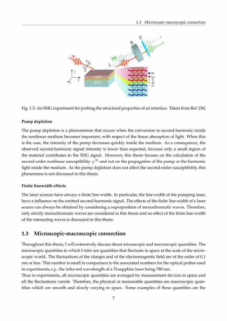
The use of the sensitivity to symmetries of SHG is not only restricted to biology and neurosciences.Surface science makes also an extensive use of SHG for the characterization of thin films [23–25],interfaces [26–29], surfaces [30–34], and more recently monolayer materials as TMDs [15, 19], seeFig. 1.2(c). In these cases, the second-harmonic generation is used as an in situ, non-invasive andnon-destructive probe. Various techniques have been developed, allowing real-time monitoring ofsemiconductors growth, surface reconstruction determination, etc.The experimental set-up is sketched in Fig. 1.3. A great force of SHG is that in experiments, onecan vary the incoming polarization, choose the angle of incidence, select the out-going polarizationor rotate the sample. This gives access to a lot of information and, going further, it is possible toidentify specific fingerprints of some structures, see, for instance for surfaces, Ref. [35]. In SHGsurface applications, the main condition is that the bulk material used is centro-symmetric. As aconsequence, the second-harmonic signal originates only from the symmetry-breaking regions asdefects, interfaces and, more importantly, surfaces.
1.2.2 Second-harmonic generation related phenomena
Some phenomena are related to the second-harmonic generation and in particular to the propagationof the pump and harmonic waves inside the medium.
6
1.3 Microscopic-macroscopic connection
Fig. 1.3: An SHG experiment for probing the structural properties of an interface. Taken from Ref. [36]
Pump depletion
The pump depletion is a phenomenon that occurs when the conversion to second-harmonic insidethe nonlinear medium becomes important, with respect of the linear absorption of light. When thisis the case, the intensity of the pump decreases quickly inside the medium. As a consequence, theobserved second-harmonic signal intensity is lower than expected, because only a small region ofthe material contributes to the SHG signal. However, this thesis focuses on the calculation of thesecond-order nonlinear susceptibility χ(2) and not on the propagation of the pump or the harmoniclight inside the medium. As the pump depletion does not affect the second-order susceptibility, thisphenomena is not discussed in this thesis.
Finite linewidth effects
The laser sources have always a finite line-width. In particular, the line-width of the pumping laser,have a influence on the emitted second-harmonic signal. The effects of the finite line-width of a lasersource can always be obtained by considering a superposition of monochromatic waves. Therefore,only strictly monochromatic waves are considered in this thesis and no effect of the finite line-widthof the interacting waves is discussed in this thesis.
1.3 Microscopic-macroscopic connection
Throughout this thesis, I will extensively discuss about microscopic and macroscopic quantities. Themicroscopic quantities to which I refer are quantities that fluctuate in space at the scale of the micro-scopic world. The fluctuations of the charges and of the electromagnetic field are of the order of 0.1nm or less. This number is small in comparison to the associated numbers for the optical probes usedin experiments; e.g., the infra-red wavelength of a Ti:sapphire laser being 780 nm.Thus in experiments, all microscopic quantities are averaged by measurement devices in space andall the fluctuations vanish. Therefore, the physical or measurable quantities are macroscopic quan-tities which are smooth and slowly varying in space. Some examples of these quantities are the
7

Chapter 1. Introduction
transmission/reflection coefficients, the absorption spectra or the loss functions. In the case of thegeneration of second-harmonic by reflection of light on a surface, the measurable quantities are thereflection coefficients, as explained more in details in Chap. 2.The measurable quantities, or macroscopic quantities, are entirely determined by the microscopicquantities. The procedure which links the microscopic quantities (described by microscopic Maxwellequations, see Eqs. B.1) to the macroscopic quantities (macroscopic Maxwell equations, Eqs. B.9) iscalled the macroscopic averaging.The question of the definition of this averaging procedure is not simple and requires some care. Dif-ferent definitions can be found in the literature, e.g., Refs. [37–40]. As pointed out in Ref. [39], thisprocedure depends on the nature of the system. In this thesis we adopt the approach of R. Del Soleand E. Fiorino [38] for dealing with periodic systems.
1.3.1 Local-fields
When applying an external electric field Eext to a dielectric material, electric dipoles are created at amicroscopic level. These dipoles are responsible for the apparition, inside the material, of an inducedfield Eind. The total electric field felt by electrons is microscopic and is thus given by these two con-tributions; E = Eext + Eind. Taking into account the effects due to the presence of the induced field,but also due to the density fluctuations or any kind of microscopic inhomogeneities, is a challengingtask. These effects are often referred as the local-field effects.In the case of bulk materials, the local-field effects have been widely studied and in particular their ef-fects on the optical properties are now well established. Their effects on optical properties of surfacesis still an open question, mainly because the theoretical description and the numerical simulations inthe case of surfaces are more intricate than for bulk materials. The abrupt change in the electronicdensity at the interface with vacuum leads to a huge variation of the electric field. As a result, strongeffects of the local field are expected, in particular in the direction perpendicular to the plane of thesurface. This thesis aims to quantify how important these effects are for the linear and the second-order optical properties of surfaces.
1.3.2 Macroscopic quantities
From a theoretical point of view, the inclusion of the local-field effects is closely related to the macro-scopic averaging mentioned previously. In this thesis, the inclusion of the local-field effects followsthe formalism of Ref. [38], which has been extended to the second-order by Luppi et al. in Ref. [41]and Huebener et al. in Ref. [42,43]. The first step in this approach is to define a perturbing field, suchas
EP = Eext +Eind,T = E−Eind,L, (1.3)
where E is the total microscopic field, Eext is the external field and Eind,T and Eind,L are respectivelythe transverse and the longitudinal components of the field induced by the external perturbation.In this thesis, I will focus on two macroscopic quantities, the macroscopic dielectric tensor andsecond-order susceptibility tensor. The macroscopic dielectric tensor is defined as the link betweenthe macroscopic first-order electric displacement and the macroscopic total electric field. In frequency
8

1.3 Microscopic-macroscopic connection
space reciprocal space, this relation reads as
D(1)M (q;ω) =
↔ǫM (q;ω)EM (q;ω). (1.4)
The macroscopic second-order susceptibility is defined as the link between three measurable quan-tities, the macroscopic second-order polarization P
(2)M and the two macroscopic incoming total elec-
tric fields EM ,
P(2)M (q;ω) =
∑
q1,q2
∫
dω1dω2↔χ(2)
M (q,q1,q2;ω1, ω2)EM (q1;ω1)EM (q2;ω2)δq,q1+q2δ(ω − ω1 − ω2).
(1.5)Note that the delta functions ensure the conservation of the energy and the conservation of the mo-mentum.
The first-order polarization is related to the perturbing electric field via the quasi-polarisability
tensor, denoted↔α(1)
. The time Fourier transform of this definition reads as [38]
P(1)(r;ω) =
∫
d3r1↔α(1)
(r, r1;ω)EP (r1;ω). (1.6)
Similarly, the second-order polarization is given by
P(2)(r;ω) =
∫
d3r1d3r2
∫
dω1dω2δ(ω − ω1 − ω2)↔α(2)
(r, r1, r2;ω1, ω2)EP (r1;ω1)E
P (r2;ω2), (1.7)
where↔α(2)
is the second-order quasi-polarisability [41]. Assuming a periodic crystal, it is possible toperform the space Fourier transform of Eq. (1.6) and Eq. (1.7)
P(1)G (q;ω) =
∑
G1
[↔α(1)
(q;ω)]
GG1EP
G1(q;ω), (1.8a)
P(2)G (q;ω) =
BZ∑
q1q2
∑
G1G2
∫
dω1dω2δq,q1+q2δ(ω − ω1 − ω2)
×[↔α(2)
(q,q1,q2;ω1, ω2)]
GG1G2EP
G1(q1;ω1)E
PG2
(q2;ω2). (1.8b)
where q, q1 and q2 are vectors in the first Brillouin zone (BZ), G, G1, and G2 are reciprocal lattice
vectors, and the notations PG(q;ω) and[
↔α(1)
(q;ω)]
GG1stand respectively for P(q + G;ω) and
↔α(1)
(q+G,q+G1;ω).
In reciprocal space, the macroscopic averaging procedure consists in keeping only the G = 0 com-ponent [44], or, following the idea of Refs. [39, 40], this procedure is defined by a projector on theaveraged part, denoted Pa, whose expression in reciprocal space is Pa = δG0.In Eqs. (1.8), the first- and second-order microscopic polarizations are explicit functions of the per-turbing field, whereas the macroscopic ones depend upon the macroscopic total electric field. To
9
Chapter 1. Introduction
express the microscopic polarizations in terms of the total electric field, we use the relation betweenthe perturbing field and the total electric field obtained from Maxwell equations [41], which reads as
EPG(q;ω) = EG(q;ω) + 4π
q+G
|q+G|PLG(q;ω), (1.9)
where PL is the longitudinal part of the polarization (see App. B.3 for the definition of the longi-tudinal and transverse parts). After some algebra that the interested reader can find detailed inRef. [41, 45], we obtain the expression of the macroscopic dielectric tensor
↔ǫM (q;ω) =
↔1 +4π
[↔α(1)
(q;ω)]
00
[
↔1 +4π
q
q
q
q
[↔α(1)
(q;ω)]
00
1− 4π[
α(1),LL(q;ω)]
00
]
, (1.10)
with α(1),LL the longitudinal-longitudinal part of↔α(1)
and of the expression of the macroscopicsecond-order susceptibility
↔χ(2)
M (q,q1,q2;ω1, ω2) =
[
↔1 +4π
[↔α(1)
(q;ω)]
00
1− 4π[
α(1),LL(q;ω)]
00
q
q
q
q
]
.[↔α(2)
(q,q1,q2;ω1, ω2)]
000:
×[
↔1 +4π
q1
q1
q1
q1
[↔α(1)
(q1;ω1)]
00
1− 4π[
α(1),LL(q1;ω1)]
00
][
↔1 +4π
q2
q2
q2
q2
[↔α(1)
(q2;ω2)]
00
1− 4π[
α(1),LL(q2;ω2)]
00
]
.
(1.11)
1.3.3 Comparison with the Lorentz model
A well-known model for the local-field correction is the Lorentz model, which has been intensivelydiscussed in the literature, see Refs. [46–48] and references therein. Therefore it is interesting tocompare the results obtained with this model to the exact results obtained above.In the Lorentz model of the local field, the local field at any point of a crystal is given by the sum ofthe applied external field and an induced field created by neighbouring dipoles
Eloc(ω) = Eext(ω) +Edip(ω),
with Edip(ω) = 4π3 P(ω) for a cubic media [46].
In that case, the polarization, up to the second-order, is given by [49]
P(ω) =[
1− 4π
3α(1)(ω)
]−1(
α(1)(ω)Eext(ω)+↔α(2)
(ω, ω1, ω2)Eloc(ω1)E
loc(ω2))
, (1.12)
where α(1) and↔α(2)
are first- and second-order polarisabilities. When neglecting the contributionof P(2) to Eloc, we obtain the expression of the macroscopic dielectric function and second-ordersusceptibility in the Lorentz model [49]
ǫLorentz(ω) = 1 + 4πα(1)(ω)[ 1
1− 4π3 α
(1)(ω)
]
, (1.13a)
10
1.4 Longitudinal-transverse and optical limit
↔χ(2)
Lorentz (ω, ω1, ω2) =[ 1
1− 4π3 α
(1)(ω)
] ↔α(2)
(ω, ω1, ω2)[ 1
1− 4π3 α
(1)(ω1)
][ 1
1− 4π3 α
(1)(ω2)
]
. (1.13b)
These expressions are very similar to the exact expressions Eq. (1.10) and Eq. (1.11), and in particular,the terms in the brackets account equally for the local-field effects in both cases. Moreover, if we as-sume the cubic symmetry, the dielectric tensor reduces to its longitudinal-longitudinal-longitudinalpart [41].
↔χ(2)
M (q,q1,q2;ω1, ω2) = ǫLLM (ω)↔α(2),LLL
(q,q1,q2;ω1, ω2)ǫLLM (ω1)ǫ
LLM (ω2), (1.14)
whereas the Lorentz model gives [50, 51]
↔χ(2)
Lorentz (ω, ω1, ω2) =
[
ǫLorentz(ω) + 2
3
]
↔α(2)
(ω, ω1, ω2)
[
ǫLorentz(ω1) + 2
3
] [
ǫLorentz(ω2) + 2
3
]
(1.15)
Interestingly, the Lorentz model is found to give very similar analytical expression of the local-fieldcorrection, compared to the exact expressions obtained from the macroscopic-microscopic connec-tion. Nevertheless, in the latter, no approximation has been introduced, in particular concerning thesymmetry of the system, whereas the Lorentz model is restricted to a cubic symmetry. Moreover,the Lorentz model contains the polarisabilities (i.e., responses to the applied external field) whereasthe the macroscopic-microscopic connection yield formulae containing the quasi-polarisabilities (i.e.,responses to the perturbing field). Note that the Lorentz model for the local field can be improved byreplacing the Lorentz factor ǫ+2
3 by a more realistic expression, see for instance, Ref. [52].Even if the Lorentz model has been used to investigate experimentally the local-field effects, e.g., ina dense atomic vapor [53], it is numerically valid only in the low-energy region, far from resonancesand is not really used in practice.
1.4 Longitudinal-transverse and optical limit
The optical limit and the dipole approximation play an important role in the ab initio description ofoptical properties. Here I report some important results, for the linear and nonlinear second-orderoptical properties, related to the optical limit, also called long-wavelength approximation.
1.4.1 Dielectric tensor
Let us consider a periodic, non-magnetic (H = B) crystal, without external charges.In the longitudinal-transverse basis (see App. B.3 for the definition of longitudinal and transversefields), the dielectric tensor reads as1
↔ǫM (q;ω) =
(
ǫLLM (q;ω) ǫLTM (q;ω)
ǫTLM (q;ω) ǫTT
M (q;ω)
)
. (1.16)
1Here ǫLLM is a scalar, ǫLT
M and ǫTLM are vectors and ǫTT
M is a 2×2 matrix.
11

Chapter 1. Introduction
Inserting the definition of the macroscopic dielectric function into Maxwell equations (see Eqs B.19)yields the equation of propagation for the macroscopic electric field
|q|2ET (q;ω) =ω2
c2↔ǫM (q;ω)E(q;ω), (1.17)
where q is the momentum of the photon.This equation gives directly the familiar normal modes [38, 39, 54]. If the electric field is purelylongitudinal (E = EL), we obtain the condition of propagation of the plasmon, ǫTL
M (q;ω) = 0.In the case of a purely transverse electric field, we obtain the dispersion relation of the photon,
|ω2 ↔ǫTT
M (q;ω)− c2q2↔1 | = 0.
It is worthwhile to notice that the dispersion relation of the photon involves only transverse com-ponents of
↔ǫM . This is in contrast with the Time-Dependent Density-Functional Theory (presented
later in Chap. 3), which gives access to the longitudinal-longitudinal (LL) part of the dielectric tensoronly. Nevertheless, we can show that the LL part of the dielectric tensor is sufficient for accessingevery interesting quantity, within the long-wavelength approximation.Let us consider the long-wavelength limit.2 This approximation corresponds to a vanishing momen-tum, q → 0. Any quantity can therefore be expanded in terms of power of q. The dipole approxima-tion corresponds to the truncation of this expansion at the lowest-order in q.
The tensors↔ǫM (q;ω) and
↔α(1)
(q,q;ω) are analytic; their limit for q → 0 does not depend on the
direction of q. Let us denote these limits↔ǫM (ω) and
↔α(1)
(ω).3
Let us now assume that the tensor↔α(1)
(ω) is diagonalisable, meaning that the crystal exhibits threeprincipal axis ni. This is the case for all the crystal classes but monoclinic and triclinic crystals [55].In the case of monoclinic and triclinic crystals, the tensor can still be diagonal, but this is not true ingeneral.In the basis of the principal axis, and within the long-wavelength limit, the dielectric tensor is found
to be diagonal, from Eq. (1.10) and using the relation ni.↔α(1)
= α(1)ii ni; with the i-th component of the
dielectric tensor ǫiiM , given by
ǫiiM (ω) = ni.↔ǫM (ω).ni =
1
1− 4παLL(ni;ω), (1.18)
whereas ǫijM (ω) = 0 for i 6= j.Thereby, the dielectric tensor and the quasi-polarisability are diagonal in the same basis, and thecomponents are given by
ǫiiM (ω) = ǫLLM (q → 0;ω),q
|q| = ni. (1.19)
2The range of validity of this approximation can be easily estimated. Assuming the lattice parameter of silicon (a0 ∼
5.4Å) as the characteristic length of the system, the long-wavelength limit corresponds to λ ≫ a0. If we choose the energyof the photon to be smaller than 22.5eV , the wavelength is already such that λ > 10a0. This approximation is perfectlysuitable for the low-energy region of the optical spectra.
3Proving the analyticity of the dielectric tensor is far from been simple or obvious, see Ref. [38].
12
1.4 Longitudinal-transverse and optical limit
Let us consider now that the tensor↔α(1)
(ω) is not diagonalisable, as it is the case for monoclinic andtriclinic symmetries. For these crystals, the components of the dielectric tensor can still be computedfrom the LL part of the dielectric tensor. To illustrate that, I take the example of a monoclinic crystalwhose basal plane is perpendicular to the z-axis. In this special case, the dielectric tensor reads as
↔ǫM (ω) =
ǫxxM (ω) ǫxyM (ω) 0
ǫxyM (ω) ǫyyM (ω) 0
0 0 ǫzzM (ω)
. (1.20)
Computing the LL part of↔ǫM (ω) for q =
nx±ny√2
gives
q.↔ǫM (ω).q =
ǫxxM (ω) + ǫyyM (ω)
2± ǫxyM (ω). (1.21)
We obtain easily that
ǫxyM (ω) =1
2
(
ǫLLM (qnx + ny√
2;ω)− ǫLLM (q
nx − ny√2
;ω))
, q → 0, (1.22)
whereas the ǫiiM (ω) elements are obtained using Eq. (1.19).Therefore, in the dipole approximation, within the long-wavelength limit, the dielectric tensor canbe entirely computed from LL calculations. It is worthwhile to notice that this result is true forany symmetry class and valid independently of the level of approximation used for computing thedielectric tensor.From the knowledge of the entire dielectric tensor in one basis, the dielectric tensor can be computedin any basis. Obviously, this result is no more valid out of the dipole approximation.
Longitudinal-transverse coupling
In the basis of the principal axis (if the dielectric tensor is diagonalisable), and within the long-wavelength limit, there is no longitudinal-transverse coupling (ǫTL
M (q → 0;ω) = 0) and no transverse-longitudinal coupling (ǫLTM (q → 0;ω) = 0). Indeed, if the macroscopic electric field is longitudinal(transverse), and propagates along (perpendicular to) a principal axis, the macroscopic electric dis-placement DM obtained is along (perpendicular to) the same principal axis, and is also longitudinal(transverse).Nevertheless, a longitudinal-transverse coupling is non-vanishing in other basis than the principalaxis basis, even if the dielectric tensor is diagonalisable;4 except for the cubic symmetry, for whichthe dielectric tensor is diagonal in any basis.
Cubic crystals
The distinction between the transverse and the longitudinal parts of the dielectric tensor in the long-wavelength limit, i.e., for a vanishing momentum, is meaningless. This can be illustrated easily with
4Also, if q 6= 0, the principal axis depend on q and are not aligned a priori with q. Therefore it is no more possible tocalculate the entire dielectric tensor from longitudinal calculations if q 6= 0.
13

Chapter 1. Introduction
the example of cubic crystals. Indeed, in any basis, as the longitudinal-transverse couplings vanish,we have the two equations
DM (q → 0;ω) =↔ǫM (ω)EM (q → 0;ω),
DTM (q → 0;ω) =
↔ǫTT
M (q → 0;ω)ETM (q → 0;ω),
q
|q| = nj (1.23)
that can be projected on the principal axis ni, with i 6= j, yielding
DT,iM (q → 0;ω) = ǫiiM (ω)ET,i
M (q → 0;ω),
DT,iM (q → 0;ω) = ǫTT,ii
M (q → 0;ω)ET,iM (q → 0;ω).
q
|q| = nj (1.24)
Using Eq. (1.18), we obtain that
ǫTT,iiM (qnj;ω) = ǫLLM (qni;ω), q → 0 and i 6= j. (1.25)
This result is valid as soon as the dielectric tensor is diagonalisable, but for cubic crystals, this relation
becomes↔ǫTT
M (q → 0;ω) = ǫLLM (q → 0;ω)↔1 , for any q, because all the directions are equivalent. This
shows that the denomination longitudinal or transverse loses its meaning in the long-wavelengthlimit. This result has been discussed by P. Noziéres and D. Pines in Ref. [56], in the special context ofthe random-phase approximation. Nevertheless, as pointed out in Ref. [57], this result is general andis not restricted to some specific approximations on the calculation of the dielectric tensor.
1.4.2 Second-order susceptibility
Similar considerations for the second-order susceptibility are beyond the scope of this thesis. Already,the link between the components of χ(2)
M and its longitudinal-longitudinal-longitudinal (LLL) part isnon-trivial. In this section, I show how it is possible to obtain the components of the second-ordersusceptibility from its LLL part only, that we can compute from Time-Dependent Density FunctionalTheory (see Chap. 3).Let us assume the analyticity of the second-order susceptibility χ(2)
M (q,q1,q2;ω, ω1, ω2) and the second-order quasi-polarisability α(2)(q,q1,q2;ω, ω1, ω2)
5. It is thus possible to define χ(2)M (ω, ω1, ω2) and
α(2)(ω, ω1, ω2) as their respective limits for q1 → 0 and q2 → 0.
The different components of↔χ(2)
M can be obtained from Eq. (1.11). There is in total four groups of com-ponents for χ(2)
M , organised by group of indices. Their calculation from the longitudinal-longitudinal-longitudinal (LLL) part of the dielectric tensor only is not obvious, and depends on the symmetriesof the crystal. We omit here the frequency dependence in second-order tensor for conciseness.
Components: χ(2)M,iii
The diagonal elements of the susceptibility tensor are given by
χ(2)M,iii = ni. χ
(2)M : ni.ni = ǫiiM (2ω)α
(2)iii ǫ
iiM (ω)ǫiiM (ω),
5The analyticity of the χ(2)M tensor will be proven in Chap. 7.
14
1.4 Longitudinal-transverse and optical limit
which are obviously related to the LLL part of susceptibility
χ(2)M,iii = χ
(2)LLLM (2q,q,q), q → 0,
q
|q| = ni.
These diagonal components can always be computed from the LLL part of the tensor, regardless ofthe symmetries of the system.
Components: χ(2)M,iij = χ
(2)M,iji
Using the relations
(ni + nj). χ(2)M : ni.nj = χ
(2)M,iij + χ
(2)M,jij ,
(ni − nj). χ(2)M : ni.nj = χ
(2)M,iij − χ
(2)M,jij ,
we can obtain2χ
(2)M,iij = χ
(2)LLLM (ni + nj,ni,nj) + χ
(2)LLLM (−ni + nj,−ni,nj) (1.27)
Therefore, the components of χ(2)M,iij = χ
(2)M,iji can always be computed from the LLL part of the tensor,
regardless the symmetries of the crystal; at the cost of computing two longitudinal responses.
Components: χ(2)M,ijj
Using q1
|q1| = ni and q2
|q2| =ni+nj√
2, we obtain that
1
2
(
χ(2)M,iij + χ
(2)M,ijj + (1 +
√2)(χ
(2)M,jji + χ
(2)M,jjj)
)
= χ(2),LLLM (q1 + q2,q1,q2, 2ω, ω;ω) (1.28)
By combining this expression with the two previous results, it is possible to calculate the componentsijj of the second-order susceptibility tensor. Note that in general, the terms on the left-hand side arenot all non-zero for the same symmetry and therefore, this equation get simpler for many of thesymmetries.
Components: χ(2)M,ijk = χ
(2)M,ikj , i 6= j 6= k
There is no simple general expression for obtaining these components from the longitudinal part ofthe second-order susceptibility tensor. However, for some symmetry classes, these components canbe easily obtained, e.g., cubic crystals. In that case, the only non-zero components are the χ(2)
M,ijk. Bychoosing q1
|q1| =q2
|q2| =q|q| =
ni+nj+nk√3
, we obtain that
χ(2)M,ijk(2ω, ω, ω) =
1
6χ(2)LLLM (2q,q,q; 2ω, ω, ω).
Obviously, the choices presented here are not unique are clever choices can be found, based on thespecific symmetries of the crystal considered.
15
Chapter 1. Introduction
1.5 Present work
The study of optical properties of surfaces is driven by one main motivation: understanding howthe presence of the surface modifies the bulk optical properties and related spectroscopic techniques.This fundamental question has many practical implications: optical spectroscopies are now usedroutinely, e.g., for monitoring and controlling of the surface growth in real time [58]; moreover, it isnow well established that physical properties of nano-scaled systems are strongly influenced by theirsurface behavior [59].
Over the last years, experimental and theoretical approaches have considerably advanced, deepen-ing our understanding of the processes occurring at the surface of materials. However, these opticalproperties result of an intricate interplay of numerous effects and achieving a correct theoretical de-scription of surfaces is far from being simple. First of all, the atomic relaxation at the interface withvacuum is responsible for a change in the electronic properties of the material, creating for instancesurface states that can be located in the gap of the material [60]. The local-field and other effects re-lated to many-particle physics, such as electron-hole interactions, occurring in all spectroscopic mea-surements must be properly included. Their precise description for surfaces is nevertheless quiteinvolved [61].
In this thesis, the optical properties of surfaces are computed using the common approach whichrelies on the super-cell technique and the slab geometry. Unfortunately, the definition of a surface
dielectric tensor (or second-order susceptibility) is still unclear, and the difference between the opticalresponse of a thin film (made of two surfaces) and the optical response of a semi-infinite system,with a single surface, has not really being investigated so far, in particular when local-field effects areincluded.
The aim of this thesis is to clarify the definition of the surface optical properties and to give thetheoretical background needed for computing linear and second-order optical properties of a singlesurface, from calculations performed in slab geometry. The Chap. 5 and Chap. 6 are dedicated tothe theory behind the calculation of the surface second-harmonic spectra in super-cell geometry, at amicroscopic level.
A macroscopic formalism, allowing us to obtain the first and second-order optical properties ofsurfaces is then developed in Chap. 7, allowing us to include the local-field effects. Chap.8 presentshow we can treat a truly isolated slab, from a periodic super-cell approach.I present in Chap 9, for the first time, ab initio calculations of the local-field effects on surface second-harmonic generation spectra. Also, an insight of the excitonic effects on the surface second-harmonicspectra is presented in Chap. 10.
Summary
As a summary, I have presented in this chapter the phenomenon of second-harmonic generation,several of its applications and some related phenomena. Then I have presented how the macroscopicquantities, directly related to quantities measured in experiments depend on the microscopic quanti-ties, fluctuating on the nanoscale. I have also discussed about the longitudinal and transverse parts of
16

1.5 Present work
the optical responses, showing in particular that within the long-wavelength limit, the longitudinalresponse to longitudinal perturbations is sufficient for describing the first- and second-order opticalproperties of any crystals. Finally, the scope and the organisation of the thesis have been presented.
17

Chapter 2. Second-harmonic generation in reflection
Despite the growing interest in SHG, the literature remains unclear concerning the derivation of thereflection coefficients, ant it is not always easy to understand what is the phenomenological treat-ment in the derivation of that coefficients, an exception been Ref. [73].The aim of this chapter is to present a comprehensive derivation of the expressions of the differentreflection coefficients, for both surface and bulk contributions, based on the work of Ref. [73].
Modelling the experiment
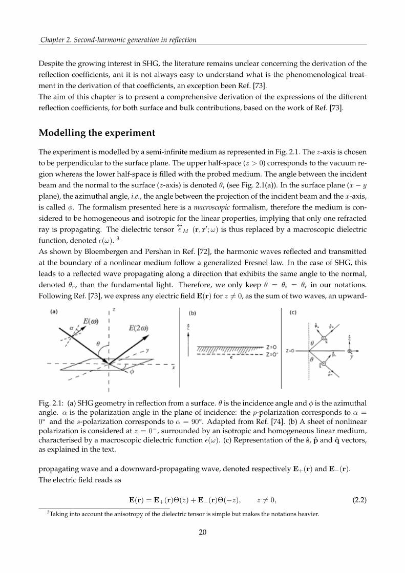
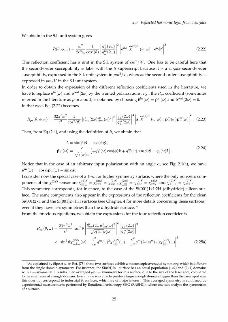
The experiment is modelled by a semi-infinite medium as represented in Fig. 2.1. The z-axis is chosento be perpendicular to the surface plane. The upper half-space (z > 0) corresponds to the vacuum re-gion whereas the lower half-space is filled with the probed medium. The angle between the incidentbeam and the normal to the surface (z-axis) is denoted θi (see Fig. 2.1(a)). In the surface plane (x− y
plane), the azimuthal angle, i.e., the angle between the projection of the incident beam and the x-axis,is called φ. The formalism presented here is a macroscopic formalism, therefore the medium is con-sidered to be homogeneous and isotropic for the linear properties, implying that only one refractedray is propagating. The dielectric tensor
↔ǫM (r, r′;ω) is thus replaced by a macroscopic dielectric
function, denoted ǫ(ω). 3
As shown by Bloembergen and Pershan in Ref. [72], the harmonic waves reflected and transmittedat the boundary of a nonlinear medium follow a generalized Fresnel law. In the case of SHG, thisleads to a reflected wave propagating along a direction that exhibits the same angle to the normal,denoted θr, than the fundamental light. Therefore, we only keep θ = θi = θr in our notations.Following Ref. [73], we express any electric field E(r) for z 6= 0, as the sum of two waves, an upward-
Fig. 2.1: (a) SHG geometry in reflection from a surface. θ is the incidence angle and φ is the azimuthalangle. α is the polarization angle in the plane of incidence: the p-polarization corresponds to α =0° and the s-polarization corresponds to α = 90°. Adapted from Ref. [74]. (b) A sheet of nonlinearpolarization is considered at z = 0−, surrounded by an isotropic and homogeneous linear medium,characterised by a macroscopic dielectric function ǫ(ω). (c) Representation of the s, p and q vectors,as explained in the text.
propagating wave and a downward-propagating wave, denoted respectively E+(r) and E−(r).The electric field reads as
E(r) = E+(r)Θ(z) +E−(r)Θ(−z), z 6= 0, (2.2)3Taking into account the anisotropy of the dielectric tensor is simple but makes the notations heavier.
20
2.1 Second-order polarization induced by incident light
where Θ(z) is the Heaviside function, Θ(z) = 1 as z > 0 and 0 elsewhere.The wave-vectors for upward/downward propagating waves are written as
qi+(ω) = q||(ω)κ+ qi⊥(ω)z,
qi−(ω) = q||(ω)κ− qi⊥(ω)z,
(2.3)
where κ is the in-plane unit vector defined by κ = cos(φ)x + sin(φ)y and i can be the medium (m)or the vacuum (v). We define q|| to be the in-plane component of the wave-vector and q⊥ the out-of-
plane component of the wave-vector. Here qi(ω)2 = ǫi(ω)(
ωc
)2and qi⊥(ω) =(
ǫi(ω)ω2
c2− q2||(ω)
)1/2=
ωc
(
ǫi(ω)− sin2(θ))1/2, qi⊥ being chosen to have Im[qi⊥] ≥ 0 and Re[qi⊥] ≥ 0 if Im[qi⊥] = 0. This conven-
tion allows us to be sure that the wave associated with qi+ is upward propagating and that the one
associated with qi− is downward-propagating.
The s and p polarizations are defined by the following unit vectors
s = κ× z,
pi± =
(q||z∓ qi⊥κ)
qi.
This is illustrated in Fig. 2.1(c). For conciseness, we omit the frequency dependence here.One can easily check that we have the following relations
s× qi± = pi
±,
qi± × pi
± = s,
pi± × s = qi
±,
(2.4)
where qi± = qi
±/qi. Thus (s; qi
+; pi+) and (s; qi
−; pi−) are direct basis.
Therefore, the wave associated with qi+ (respectively qi
−) only propagates along s and pi+ (respec-
tively pi−).
From Maxwell equations, the upward and the downward propagating waves read as
Ei+(r;ω) = (Ei
s+(ω)s+ Eip+(ω)p
i+(ω))e
iqi+(ω)r,
Bi+(r;ω) =
√
ǫi(ω)(Eip+(ω)s− Ei
s+(ω)pi+(ω))e
iqi+(ω)r,
Ei−(r;ω) = (Ei
s−(ω)s+ Eip−(ω)p
i−(ω))e
iqi−(ω)r,
Bi−(r;ω) =
√
ǫi(ω)(Eip−(ω)s− Ei
s−(ω)pi−(ω))e
iqi−(ω)r.
z 6= 0 (2.5)
2.1 Second-order polarization induced by incident light
In this section, we will give the expression of the second-order polarization induced by the incidentfield. Let us denote the incident field in the vacuum Ein(ω). The polarization of that field is denotedein(ω) which can be s or p−(ω); depending if the field is s- or p-polarised. This incident field reads as
Ein(r;ω) =(
Esin(ω)s+ Ep
in(ω)pv−(ω)
)
ei(q||(ω)r||−qv⊥(ω)z) = ein(ω)|Ein(ω)|ei(q||(ω)r||−qv⊥(ω)z). (2.6)
21

Chapter 2. Second-harmonic generation in reflection
Polarisation Reflection Transmission
s rsij(ω) =qi⊥(ω)−qj⊥(ω)
qi⊥(ω)+qj⊥(ω)tsij(ω) =
2qi⊥(ω)
qi⊥(ω)+qj⊥(ω)
p rpij(ω) =qi⊥(ω)ǫj(ω)−qj⊥(ω)ǫi(ω)
qi⊥(ω)ǫj(ω)+qj⊥(ω)ǫi(ω)tpij(ω) =
2qi⊥(ω)√
ǫj(ω)ǫi(ω)
qi⊥(ω)ǫj(ω)+qj⊥(ω)ǫi(ω)
Tab. 2.1: Fresnel coefficients in reflection and in transmission for s- and p-polarized lights.
At the interface with the medium, this field is transmitted. The change in phase and amplitude of thewave at the boundary is described by the Fresnel transmission coefficients (see Tab. 2.1). tpolij denotesthe transmission coefficient where pol is the polarization and can be s or p, and i and j can be themedium (m) or the vacuum (v). The field inside the medium, denoted Eω(r), is given by
Eω(r) =(
Esin(ω)t
svm(ω)s+ Ep
in(ω)tpvm(ω)pm
− (ω))
ei(q||(ω)r||−qm⊥ (ω)z) = eω|Ein(ω)|ei(q||(ω)r||−qm⊥ (ω)z),
(2.7)where the change in direction of the field has been taken into account by replacing qv⊥(ω) by qm⊥ (ω),pv−(ω) by pm
− (ω) and ein(ω) by eω. Here eω =[
stsvm(ω)s+ pm− (ω)tpvm(ω)pv
−(ω)]
ein(ω).This incident field in the medium, Eω, leads to the apparition of a second-order polarization in themedium, denoted P(2), which is given by
P(2)(r; 2ω) =
∫ 0
−∞d3r′
∫ 0
−∞d3r′′
↔χ(2)
(r, r′, r′′;ω, ω) : Eω(r′)Eω(r′′), (2.8)
where↔χ(2)
is the macroscopic second-order susceptibility of the medium.Introducing the expression of the field inside the medium, Eω, in Eq. (2.8) gives directly
P(2)(r; 2ω) =
∫ 0
−∞d3r′
∫ 0
−∞d3r′′
↔χ(2)
(r, r′, r′′;ω, ω) : eωeω|Ein|2ei(q||(ω)(r′||+r′′||)−qm⊥ (ω)(z′+z′′))
. (2.9)
2.2 Harmonic field inside the material
In this section, we consider the non-linearity to originate only from the surface region. The bulkcontribution to the generation of second-harmonic is treated later in Sec. 2.4. The expression of thepolarization Eq. (2.9) is general and no approximation has been introduced at that stage. FollowingRef. [73], instead of using Eq. (2.9), we consider a second-order polarization having the followingform
P(2)(r; 2ω) =↔χ(2)S
(ω, ω) : eωeω|Ein|2e2i(q||(ω)r||−qm⊥ (ω)z)δ(z − z0), (2.10)
where the second-order susceptibility is replaced by a second-order surface susceptibility↔χ(2)S
, as-sumed to be local and homogeneous in the plane of the surface. Moreover, the surface polarization isassumed to be a polarization sheet located at z = z0. This is where the phenomenological treatment
22

2.2 Harmonic field inside the material
stems. In order to ease notations, we define the quantity P(2ω) as
P(2)(r; 2ω) = P(2ω)e2i(q||(ω)r||−qm⊥ (ω)z)δ(z − z0), (2.11)
where P(2ω) =↔χ(2)S
(ω, ω) : eωeω|Ein(ω)|2.This second-order polarization becomes a source term in Maxwell equations that leads to the second-harmonic field created at the surface of the medium. The reflected harmonic light will thus be givenby the solution of the upward-propagating second-harmonic wave in presence of the second-orderpolarization as a source term.As pointed out by Mizrahi et al. [73], the position of the polarization sheet (z0 = 0− or z0 = 0+) onlyresults in a change of the normalisation factor in front of the expression of the reflection coefficients,
and does not modify the weight of the different components of the↔χ(2)S
tensor in the expression ofthe reflection coefficients. Throughout this thesis, I use formulae derived for a second-order polar-ization sheet located at z0 = 0−.From the macroscopic Maxwell equations (B.9), without magnetisation and in presence of a polariza-tion of the form Eq. (2.11), we get the following set of equations
∇×B(r; 2ω)− iΩǫ(2ω)E(r; 2ω) = 4πiΩP(2)(r; 2ω),
∇×E(r; 2ω)− iΩB(r; 2ω) = 0,(2.12)
where Ω = 2ωc .
The physical solution of the Maxwell equations inside the medium (which excludes exponentiallydiverging waves) has the following form
E2ω(r) =[
Em+ (2ω)Θ(z − z0)e
−iqm⊥ (2ω)z0 +Em− (2ω)Θ(z0 − z)eiq
m⊥ (2ω)z0 + E(2ω)δ(z − z0)
]
eiq||(2ω)r|| ,
(2.13a)
B2ω(r) =[
Bm+ (2ω)Θ(z − z0)e
−iqm⊥ (2ω)z0 +Bm− (2ω)Θ(z0 − z)eiq
m⊥ (2ω)z0 + B(2ω)δ(z − z0)
]
eiq||(2ω)r|| .
(2.13b)
We now search for the coefficients Ems±(2ω) and Em
p±(2ω) of Eq. (2.5), considering the following rela-tions
E = Ess+ Eκκ+ E⊥z,∇Θ(z − z0) = zδ(z − z0),
∇δ(z − z0) = zδ′(z − z0),
(2.14)
with δ′ being the derivative of the Dirac δ distribution. Considering that different orders of singular-ities ( δ and δ′ ) must cancel separately, we obtain from the equation ∇×E(r; 2ω)− iΩB(r; 2ω) = 0,
Emp+ + Em
p− + iq||q
m
qm⊥Ez − i
Ωqm
qm⊥Bs = 0,
Ems+ − Em
s− − iΩBκ = 0,
Eκ = Es = B⊥ = 0.
(2.15)
23
Chapter 2. Second-harmonic generation in reflection
Doing the same for the equation ∇×B(r; 2ω)−iΩǫ(2ω)E(r; 2ω) = 4πiΩP(r; 2ω) leads to the relations
Emp+ − Em
p− = −4πiΩ
ǫ1/2Pκ,
Ems+ + Em
s− = 4πiΩqm
ǫ1/2qm⊥Ps,
E⊥ = −1
ǫP⊥,
Bs = Bκ = 0.
(2.16)
Putting everything together leads to the expression of the wanted coefficients
Ems±(2ω) = Em
s (2ω) =2πiΩ2
qm⊥ (2ω)s.P(2ω),
Emp±(2ω) =
2πiΩ2
qm⊥ (2ω)p±(2ω).P(2ω).
(2.17)
2.3 Reflected harmonic light from a surface
Knowing the expression of the upward-propagating second-harmonic field, we can now look at theexpression of the reflected harmonic light in the vacuum. Assuming the expression Eq. (2.17) for thecoefficients of the second-harmonic field, the electric field oscillating at the frequency 2ω and inducedin the medium, denoted E2ω(r), reads as
E2ω(r) =2πiΩ2
qm⊥ (2ω)P(2ω)ei(q||(2ω)r||−qm⊥ (2ω)z). (2.18)
At the interface with the vacuum, this upward-propagating field is transmitted into the vacuum,yielding the field Eout(r; 2ω); which is the second-harmonic field measured during the experiment.We obtain that
Eout(r; 2ω) =2πiΩ2
qm⊥ (2ω)e2ωP(2ω)ei(q||(2ω)r||−qm⊥ (2ω)z), (2.19)
with e2ω = eout(2ω)[
stsmv(2ω)s+ pv+(2ω)t
pmv(2ω)pm
+ (2ω)]
, eout(2ω) being the measured polariza-tion. The intensity of the second-harmonic field in the vacuum is finally given by
Iout(2ω) =c
2π|Eout(2ω)|2 =
8π3
c
∣
∣
∣
∣
∣
Ω2
qv⊥(2ω)
∣
∣
∣
∣
∣
2 ∣∣
∣
∣
qv⊥(2ω)
qm⊥ (2ω)
∣
∣
∣
∣
2 ∣∣
∣
∣
e2ω.↔χ(2)S
(ω, ω) : eωeω∣
∣
∣
∣
2
I2in(ω). (2.20)
Inserting the definition of the Ω and qv⊥(2ω), the general form of the reflection coefficients is found tobe
R(θ, φ, ω) =32π3ω2
c31
cos2(θ)
∣
∣
∣
∣
qv⊥(2ω)
qm⊥ (2ω)
∣
∣
∣
∣
2 ∣∣
∣
∣
e2ω.↔χ(2)S
(ω, ω) : eωeω∣
∣
∣
∣
2
. (2.21)
24
2.3 Reflected harmonic light from a surface
We obtain in the S.I. unit system gives
R(θ, φ, ω) =ω2
2c3ǫ0
1
cos2(θ)
∣
∣
∣
∣
qv⊥(2ω)
qm⊥ (2ω)
∣
∣
∣
∣
2 ∣∣
∣
∣
e2ω.↔χ(2)S
(ω, ω) : eωeω∣
∣
∣
∣
2
. (2.22)
This reflection coefficient has a unit in the S.I. system of cm2/W . One has to be careful here thatthe second-order susceptibility is label with the S superscript because it is a surface second-ordersusceptibility, expressed in the S.I. unit system in pm2/V , whereas the second-order susceptibility isexpressed in pm/V in the S.I unit system.In order to obtain the expression of the different reflection coefficients used in the literature, wehave to replace ein(ω) and eout(2ω) by the wanted polarizations; e.g., the Rps coefficient (sometimesreferred in the literature as p-in s-out), is obtained by choosing ein(ω) = pv
−(ω) and eout(2ω) = s.In that case, Eq. (2.22) becomes
Rps(θ, φ, ω) =32π3ω2
c31
cos2(θ)
∣
∣tsmv(2ω)tpvm(ω)2
∣
∣
2∣
∣
∣
∣
qv⊥(2ω)
qm⊥ (2ω)
∣
∣
∣
∣
2 ∣∣
∣
∣
s.↔χ(2)S
(ω, ω) : pm− (ω)pm
− (ω)
∣
∣
∣
∣
2
. (2.23)
Then, from Eq.(2.4), and using the definition of κ, we obtain that
s = sin(φ)x− cos(φ)y,
pm± (ω) =
c√
ǫ(ω)ω
[
∓qm⊥ (ω) cos(φ)x∓ qm⊥ (ω) sin(φ)y + q||(ω)z]
.(2.24)
Notice that in the case of an arbitrary input polarization with an angle α, see Fig. 2.1(a), we haveein(ω) = cosαpv
−(ω) + sinαs.I consider now the special case of a 4mm or higher symmetry surface, where the only non-zero com-ponents of the χ(2)S tensor are χ(2)S
‖‖⊥ = χ(2)Sxxz = χ
(2)Syyz , χ(2)S
⊥‖‖ = χ(2)Szxx = χ
(2)Szyy and χ(2)S
⊥⊥⊥ = χ(2)Szzz .
This symmetry corresponds, for instance, to the case of the Si(001)1x1:2H (dihydride) silicon sur-face. The same components also appear in the expressions of the reflection coefficients for the cleanSi(001)2×1 and the Si(001)2×1:H surfaces (see Chapter. 4 for more details concerning these surfaces),even if they have less symmetries than the dihydride surface. 4
From the previous equations, we obtain the expressions for the four reflection coefficients
Rpp(θ, ω) =32π3ω2
c3tan2 θ
∣
∣
∣
∣
∣
tpmv(2ω)tpvm(ω)2
√
ǫ(2ω)ǫ(ω)
∣
∣
∣
∣
∣
2 ∣∣
∣
∣
qv⊥(2ω)
qm⊥ (2ω)
∣
∣
∣
∣
2
×∣
∣
∣
∣
sin2 θχ(2)S⊥⊥⊥(ω) +
c2
ω2qm⊥ (ω)2χ
(2)S⊥‖‖ (ω)−
c2
ω2qm⊥ (2ω)qm⊥ (ω)χ
(2)S‖‖⊥ (ω)
∣
∣
∣
∣
2
, (2.25a)
4As explained by Sipe et al. in Ref. [75], these two surfaces exhibit a macroscopic averaged symmetry, which is differentfrom the single domain symmetry. For instance, the Si(001)2×1 surface has an equal population (1×2) and (2×1) domainswith a m-symmetry. It results in an averaged p2mm symmetry for this surface, due to the size of the laser spot, comparedto the small size of a single domain. Even if one was able to produce large enough domain, bigger than the laser spot size,this does not correspond to industrial Si surfaces, which are of major interest. This averaged symmetry is confirmed byexperimental measurements performed by Rotational Anisotropy SHG (RASHG), where one can analyse the symmetriesof a surface.
25

Chapter 2. Second-harmonic generation in reflection
Rsp(θ, ω) =32π3ω2
c3tan2 θ
∣
∣
∣
∣
∣
tpmv(2ω)tsvm(ω)2√
ǫ(2ω)
∣
∣
∣
∣
∣
2 ∣∣
∣
∣
qv⊥(2ω)
qm⊥ (2ω)
∣
∣
∣
∣
2 ∣∣
∣
∣
χ(2)S⊥‖‖ (ω)
∣
∣
∣
∣
2
, (2.25b)
Rps(ω) = Rss(ω) = 0. (2.25c)
Due to the symmetries, the two coefficients associated with a measured s-polarization are zero. More-over, Rpp andRsp do not depend on the azimuthal angle φ, due to the in-plane isotropy of the surface(4mm symmetry class). This last point has been used in Ref. [76, 77] to separate the contributions tothe signal from the surface and from the bulk part of the material, for the dihydride surface. Thecareful reader will also note that theRpp coefficient contains contributions from all the non-zero com-ponents. The expressions of these coefficients, obtained without assuming any symmetry, and in thecase of other symmetries are given in App. C.
2.4 Bulk contribution
So far, I do not have discussed the contribution coming from the bulk part of the material to thereflected signal. There are three different cases in which the bulk can contribute to the reflected har-monic waves: i) The case of the non-centrosymmetric bulk. In that case, the signal is dominated bythe bulk dipolar contribution. ii) The case of centrosymmetric material, where the dipolar contribu-tion vanishes, but not the quadrupolar contribution. The quadrupolar contribution has been foundnon-negligible in some cases; compared to the surface signal [78–80]. iii) A material, having or notthe inversion symmetry, under an electric field, and therefore producing an Electric Field InducedSecond-Harmonic (EFISH) contribution. This last point will not be discuss here but is discussed ex-tensively in Ref. [81]. All these cases can be treated using the same approach than presented in theprevious sections of this chapter. Following Ref. [73], I first consider a general expression for thenonlinear polarization in the medium, given by
P(2)(r; 2ω) =↔χ(2)
(ω, ω) : Eω(r)Eω(r) + γB(ω)∇[Eω(r).Eω(r)], (2.26)
where Eω(r) is the fundamental electric field inside the material,↔χ(2)
is the bulk second-order suscep-tibility tensor and γB serves for describing the quadrupolar response of the bulk part of the material.Here I have chosen a simple expression for the quadrupolar contribution, where only the isotropicpart has been considered. More precise expressions for the quadrupolar part can be obtained byadding extra terms, as done in Ref. [64] for instance.Introducing the expression of Eω(r) in the expression of the polarization gives
P(2)(r; 2ω) =
(
↔χ(2)
(ω, ω) + γB(ω)[
2iq‖(ω)κ− 2iqm⊥ (ω)z]
)
: eωeω|Ein|2e2i(q||(ω)r||−qm⊥ (ω)z). (2.27)
As explained in Ref. [73], this polarization can be seen as the sum of individual sheets of polarization,as introduced previously, located at a distance z from the surface. This allows us to use the same for-malism as introduced previously for describing the harmonic field generated inside the medium. Atthe interface with the vacuum, the field is modified according to the Fresnel coefficients. The electric
26
2.4 Bulk contribution
field that reaches the detector is thus Eout(z; 2ω) = Eout(z = 0+; 2ω)eiqv⊥(2ω)z = Eout(2ω)e
iqv⊥(2ω)z ,with
Eout(2ω) =2πiΩ2
qm⊥ (2ω)e2ω
∫ 0
−∞dz′e−iqm⊥ (2ω)z′P(2)(z′; 2ω)
=2πiΩ2
qm⊥ (2ω)e2ω
(
i↔χ(2)
(ω, ω)− 2γB(ω)[
q‖(ω)κ− qm⊥ (ω)z]
qv⊥(2ω) + 2qv⊥(ω)
)
: eωeω|Ein|2e2iq||(ω)r||
where e−iqm⊥ (2ω)z′ describes the propagation in the medium from the polarization sheet located at −z′to the interface at 0−. The second line comes from the fact that we consider an absorbing medium (seeRef. [73]). The coefficients are identical to the one defined in the case of a surface polarization. In thefollowing, I focus on the example of a cubic symmetry for a medium that lack inversion symmetry.This is for instance the case of GaAs and the expression presented bellow has been used in Ref. [63]for extracting the xyz component from its experimental reflection spectrum. The contribution of thequadrupolar term in a centro-symmetric material can be obtained similarly.In the case of a cubic material, the second-order susceptibility has only one non-zero component,χ(2)xyz . The reflection coefficients in that case have the general form
R(θ, φ, ω) =32π3ω2
c31
cos2 θ
∣
∣
∣
∣
qv⊥(2ω)
qm⊥ (2ω)[qm⊥ (2ω) + 2qm⊥ (ω)]
∣
∣
∣
∣
2 ∣∣
∣
∣
e2ω↔χ(2)
(ω, ω) : eωeω∣
∣
∣
∣
2
, (2.28)
or in the S.I. unit sytem5,
R(θ, φ, ω) =ω2
2c3ǫ0
1
cos2 θ
∣
∣
∣
∣
qv⊥(2ω)
qm⊥ (2ω)[qm⊥ (2ω) + 2qm⊥ (ω)]
∣
∣
∣
∣
2 ∣∣
∣
∣
e2ω↔χ(2)
(ω, ω) : eωeω∣
∣
∣
∣
2
. (2.29)
The expressions of the four usual reflection coefficients are given in App. C.
Conclusion
In this chapter, I have reported the derivation of the expressions of the generalized reflection coef-ficients. They describe how the second-harmonic light is generated by reflection of a fundamentallight on a surface. We have seen that a second-order polarization is induced by the incident light andhow that polarization, acting as a source term for the Maxwell equations, yields a second-harmonicfield, reflected from the surface. This formalism allows us to treat both bulk and surface dipolar con-tributions and also the other bulk contributions such as the bulk quadrupolar and the EFISH; for anycombination of input and output polarizations of the light. Moreover, if we want to obtain the con-tributions coming from the bulk medium and its surface at the same time, the reflection coefficientscan be obtained by the mean of Eq. 2.19, using an effective polarization given by
Peff(2ω) =
(
↔χ(2)S
(ω, ω) +i↔χ(2)
(ω, ω)− 2γB(ω)[
q‖(ω)κ− qm⊥ (ω)z]
[qm⊥ (2ω) + 2qm⊥ (ω)]
)
: eωeω|Ein|2. (2.30)
5Notice that in this expression,↔χ
(2)
is a bulk second-order susceptibility, expressed in pm/V in the S.I. unit system.
27

Chapter 2. Second-harmonic generation in reflection
To conclude, we have presented here a simple model for the generation of second-harmonic in reflec-tion from surfaces. Some features are missing and can be added to account, for instance, for multiplereflections from a cover oxide layer [82], the anisotropy of the linear medium or corrections to theFresnel reflection coefficients due to the presence of the surface [83].Nevertheless, the difficulty here is not contained in such possible improvements of the descriptionof the reflection of light but in a quantitative ab initio description of the macroscopic second-orderresponse function of the surface part of the material. In the next chapter, I briefly present the (time-dependent) density-functional theory and how this framework allows us to compute the second-
order susceptibility tensor↔χ(2)
from the perturbation theory.
28

3. (Time-Dependent) Density-FunctionalTheory in a nutshell
Sometimes one can improve the theories in the sense of discovering aquicker, more efficient way of doing a given calculation.
Sir John Anthony Pople, Nobel prize co-winner for the DFT
This chapter aims to review the fundamental background of the Density-Functional Theory (DFT)and Time-Dependent Density-Functional theory (TDDFT). This exact theories give respectively ac-cess to the ground-state and excited states of the many-body systems. The ground-state gives accessto numerous properties of the system such as the total energy, the electron density or the correlationfunctions.The optical properties, as many other properties, are not properties of the ground-state and requirethe knowledge of the excited states. For obtaining the excited states, one can use the Time-DependentDensity-Functional Theory (TDDFT), which has been proven to give reliable results for the calcula-tion of linear and nonlinear optical properties of bulk materials [84] and interfaces [29].If the interaction that drives the system out of its ground-state is small, the time-dependent pertur-bation theory can simplify the task associated to calculation of optical properties.This chapter is organised as follows. As excitations in the frame of this thesis are restricted to smallperturbations of the entire system, I first discuss how within the framework of time-dependent per-turbation theory, one can obtain the linear and the second-order response functions, describing thelinear and nonlinear optical properties. Then I briefly review the static and time-dependent Density-Functional Theory, as well as some common approximations. Finally, some numerical details relatedto the calculation performed during this thesis are presented.
3.1 Time-dependent perturbation theory
In perturbation theory, the interaction between light and electrons is treated as a perturbation. Thisperturbation induces a response inside the system. More precisely it induces a current and a density,respectively denoted jind and nind.
29

Chapter 3. (Time-Dependent) Density-Functional Theory in a nutshell
3.1.1 Induced current and induced density
As it is customary for a perturbative approach, the two induced quantities are expended in powerof the perturbation. The first-order terms describe the linear response of the system and are denotedrespectively j
(1)ind and n
(1)ind. Similarly, the second-order induced current and density, denoted j
(2)ind and
n(2)ind, describe the nonlinear second-order phenomena, such as second-harmonic generation.
We start by considering the total single-electron Hamiltonian H(t) that reads as
H(t) = H0 +HI(t),
where H0 is the unperturbed time-independent Hamiltonian and HI(t) is the time-dependent inter-action Hamiltonian due to the interaction of the electrons with the electromagnetic field. We switchon the perturbation adiabatically at t0 = −∞. The interaction Hamiltonian is made of a first-ordercontribution plus a second-order contribution, such as HI(t) = H
(1)I (t) +H
(2)I (t), with [44]
H(1)I (t) =
∫
d3rn(r)φP (r, t)− 1
c
∫
d3rj(r)AP (r, t), (3.1a)
H(2)I (t) =
1
2c2
∫
d3rn(r)AP (r, t)2, (3.1b)
where φP is the scalar potential, AP the vector potential, and n and j are respectively the density andthe current operators, defined by
n(r) =∑
i
δ(r− ri), (3.2a)
j(r) =1
2
∑
i
[piδ(r− ri) + δ(r− ri)pi] . (3.2b)
To obtain the induced current and the induced density, it is necessary to evaluate the expectation val-ues of these operators with respect to the Schrödinger many-body wave-functions Ψ(t). For derivingthese expressions, it is common in perturbation theory to use the interaction representation, wherethe wave-functions ΨI(t) are given by
ΨI(t) = eiH0(t−t0)Ψ(t0), i∂
∂tΨI(t) = eiH0(t−t0)HIe
−iH0(t−t0)ΨI(t) = HI,IΨI(t), (3.3)
where HI,I describes the interaction in interaction representation.From perturbation theory, up to second-order, using the Baker-Hausdorff theorem [85], we obtainthat
jind(r, t) = 〈ΨI(t)|jind(r, t)|ΨI(t)〉
= 〈jind(r, t)〉 − i
∫ t
t0
dt′〈[
jind(r, t), HI,I(t′)]
〉 −∫ t
t0
dt′∫ t′
t0
dt′′〈[[
jind(r, t), HI,I(t′)]
, HI,I(t′′)]
〉, (3.4)
where we use the notation 〈O〉 = 〈Ψ0(t0)|O|Ψ0(t0)〉, Ψ0 being the ground-state many-body wave-function. A similar formula holds for the induced density. From the general expression of the in-
30
3.1 Time-dependent perturbation theory
duced current, it is easy to obtain the expression of, says, the first-order induced current [44]
j(1)ind(r, t) = −1
c〈n(r)〉AP (r, t) +
i
c
∫
d3r′∫
dt′θ(t− t′)〈[
jI(r, t), jI(r′, t′)
]
〉AP (r′, t′)
− i
∫
d3r′∫
dt′θ(t− t′)〈[
jI(r, t), nI(r′, t′)
]
〉φP (r′, t′).
The expressions of the second-order induced current or first- and second-order induced density arenot shown for conciseness, but can be obtained in a similar way.It is interesting to define response functions [44], which link the perturbation to the response andcontains all the physics that we want to describe. At the first- and the second-order, the responsefunctions have the general form [41, 44]
χAB(r, t, r′, t′) = iθ(t− t′)〈
[
AI(r, t), BI(r′, t′)
]
〉, (3.6a)
χABC(r, t, r1, t1, r2, t2) = θ(t− t1)θ(t− t2)T 〈[[
AI(r, t), BI(r1, t1)]
, CI(r2, t2)]
〉, (3.6b)
where A, B and C can be j or n, and T is the time-ordering operator. For instance, if we chooseA = B = C = j, we get at first-order the so-called current-current response function χjj and atsecond-order the current-current-current response function χjjj. From Eqs. (3.6), it is obvious that theresponse functions are causal and that
χAB(r, t, r′, t′) = 0 for t′ > t,
χABC(r, t, r1, t1, r2, t2) = 0 for t1 > t or t2 > t.
Also, if we replace the operators in Eqs. (3.6), by their Schrödinger representation, we obtain that theresponse functions are invariant by translation in time
χAB(r, t, r′, t′) = χAB(r, r
′, t− t′) for t′ > t,
χABC(r, t, r1, t1, r2, t2) = χABC(r, r1, r2, t− t1, t− t2) for t1 > t or t2 > t.
In total there are 4 response functions at the first-order and 8 at the second-order, leading to rela-tively complex expressions for the induced quantities. However it is possible to rearrange all theterms, using gauge-invariance [44, 45], and by introducing the expression of the perturbing electricfield EP .1 After some algebra that the interested reader can find in Ref. [45], the induced current andthe induced density are given in frequency space by 2
j(1)ind(r;ω) =
i
ω〈n(r)〉EP (r;ω)− i
ω
∫
d3r′χjj(r, r′;ω)EP (r′;ω), (3.9a)
1The perturbing field is given by
EP (r;ω) =
iω
cA
P (r;ω)−∂
∂rφP (r;ω).
2For obtaining these expressions, one must first use the fact that χAB(r, t, r′, t′) = χAB(r, r
′, t − t′) andχABC(r, t, r1, t1, r2, t2) = χABC(r, r1, r2, t− t1, t− t2). Indeed, in absence of strong perturbing field, the system is station-ary in time and the response depends only on the time difference between the moment of the response and the impositionof perturbation [54].
31
Chapter 3. (Time-Dependent) Density-Functional Theory in a nutshell
j(2)ind(r;ω) = − 1
2ω1ω2
∫
d3r1d3r2
∫
dω1dω2δ(ω − ω1 − ω2)EP (r1;ω1)E
P (r2;ω2)
×[
χjjj(r, r1, r2;ω1, ω2) + 2χρj(r, r1;ω1)δ(r− r2)−iδ(r− r2)
(ω1 + ω2)
∂
∂r1χjj(r, r1;ω1 + ω2)
]
, (3.9b)
n(1)ind(r;ω) =
i
ω
∫
d3r′χρj(r, r′, ω)EP (r′;ω), (3.9c)
n(2)ind(r;ω) =
i
2
∫
d3r1
∫
dω1dω2δ(ω − ω1 − ω2)
(ω1 + ω2)ω1ω2
∂
∂r1χρj(r, r1;ω)E
P (r1;ω1).EP (r1;ω2)
− 1
2
∫
d3r1d3r2
∫
dω1dω2δ(ω − ω1 − ω2)
ω1ω2χρjj(r, r1, r2;ω1, ω2)E
P (r1;ω1)EP (r2;ω2). (3.9d)
Only few response functions, among all possible response functions, are finally involved in theexpressions of the induced current and the induced density. Indeed, the first-order responses aredescribed only by the two response functions χjj and χρj, whereas one must also include χjjj and χρjj
in order to describe the second-order responses. All the other response functions can be obtainedfrom these four ones. With these expressions, one can describe any perturbation of the system atfirst- and second-order.
3.2 Density-Functional Theory (DFT)
Before presenting the Density-Functional Theory, I start with the quantum description of system anda basic approximation, commonly used in quantum mechanics, the Born-Oppenheimer approxima-tion. Then I review the basements of the Density-Functional Theory (DFT), which are the Hohenberg-Kohn theorems and the Kohn-Sham method.
3.2.1 Many-body Hamiltonian
In this thesis, the matter is quantified and the light is treated classically. The starting point of thequantum treatment of the matter is to consider a system of interacting electrons and nuclei. Thesystem is considered to be non-magnetic. Relativistic and quantum electrodynamics effects are ne-glected. The static many-body Hamiltonian associated to such a system is given by
H(r,R,p,P) =∑
i
pi2
2me−∑
i,I
ZIe2
|ri −RI|+
1
2
∑
i 6=j
e2
|ri − rj|+∑
I
PI2
2MI+
1
2
∑
I 6=J
ZIZJe2
|RI −RJ|, (3.10)
where the electrons are represented by the coordinates ri, the momenta pi, and a mass me. Nucleiare represented by the coordinates RI, the momenta PI, and a mass MI .The fundamental Hamiltonian can be written as the sum of the different contributions
H = Te + VeN + Vee + TN + VNN , (3.11)
32
3.2 Density-Functional Theory (DFT)
where Te and TN are the kinetic energies of the electrons and of the nuclei respectively, Vee is theelectron-electron Coulomb interaction
Vee =1
2
∑
i 6=j
e2
|ri − rj|, (3.12)
that excludes the self-interaction term (i 6= j) and VeN and VNN are electron-nuclei and nuclei-nucleiCoulomb interactions.The task associated with solving the many-body problem represented by Eq. (3.10) is too complicatedto be treated numerically even for a small system of few ten of electrons. Therefore some approxi-mations are required. One excellent approximation for many purposes, and especially for all thecalculations of this thesis, is the well-known Born-Oppenheimer approximation [86].
Born-Oppenheimer approximation
The fundamental Hamiltonian given by Eq. (3.10) treats at the same footing electrons and nuclei.Nevertheless, they are quite different and in particular the mass of a proton (mp ∼ 1.67.10−27kg)is about 1800 times bigger than the mass of the electron (me ∼ 9.31.10−31kg). The approximationintroduced in 1927 by Born and Oppenheimer [86] consists in decoupling the motion of electronsand nuclei and to assume that the motion of the nuclei is slow in comparison to that of the electrons.The nuclei are thus considered to be fixed or frozen, giving also the name of adiabatic approximation forthe Born-Oppenheimer approximation. As the mass of nuclei is set to infinity, the kinetic energy ofnuclei is zero. The eigenvalue problem to solve, assuming the Born-Oppenheimer approximation, isgiven by
He(r,R,p,P)ϕR(r) = ERϕR(r), (3.13)
where ϕR(r) are the wave-functions of the electrons assuming fix nuclei and He(r,R,p,P) =
Te + Vee + VeN . This equation describes a system of interacting electrons in presence of an externalpotential due to the frozen nuclei at positions R.Using the Born-Oppenheimer approximation, we turn the many-body problem described by Eq. (3.10)into a many-electron problem represented by Eq. (3.13); which still represents a formidable problemto solve. In the following, I always assume the Born-Oppenheimer approximation. The nuclei po-sitions are parameters of the calculations and the subscript R is now omitted for conciseness. TheHamiltonian representing the electronic problem will be written from now on as
He(r,p) =∑
i
pi2
2+∑
i
Vext(ri) +1
2
∑
i 6=j
1
|ri − rj|, (3.14)
with Vext the electrons-nuclei interaction potential.
3.2.2 Hohenberg-Kohn theorems
In their paper [87] published in 1964, Hohenberg and Kohn laid the foundations of the Density-Functional Theory (DFT). They proved two theorems that are presented here. The proofs of those
33

Chapter 3. (Time-Dependent) Density-Functional Theory in a nutshell
two theorems are not reported here but a detailed proof can be found, for instance, in Refs. [88, 89].
The density as the key quantity
The first theorem of Hohenberg and Kohn states the following: [89]The ground-state density n0(r) of a bound system of interacting electrons in some external potential Vext(r)
determines this potential uniquely.
This theorem implies that the ground-state wave-function and thus the expectation value of anyphysical observable is a unique functional of the electron density n(r). Unique means here: de-fined up to an additive constant. Originally this theorem has been demonstrated for non-degeneratestates, then it has been extended to a wide class of systems including systems with degenerate states(Levy [90] and Leibs [91]), spin-polarised systems (spin density-function theory, Ref. [92, 93]). Thistheorem has also been extended to finite temperature by Mermin [94], thus proving that entropy,specific heat, etc. are functionals of the equilibrium density [88].
The functional that determines the ground-state
The second theorem, directly related to the first one, states that:The total energy is a functional of the electronic density, which is minimized by the ground-state density.
The total energy for a given density n(r) is
Etot[n] = 〈Ψ|Te + Vee + Vext|Ψ〉 = FHK [n] +
∫
d3rVext(r)n(r), (3.15)
where Te, Vee and Vext have been defined previously. Here, FHK [n] is a universal functional in the sensethat it does not depends on the external potential felt by electrons. It is important to note that thissecond theorem does not tell us how to find the total energy. It is also remarkable to note that thistheorem can be seen as an exact formulation of the semi-classical Thomas-Fermi theory, proposed in1927, where all the properties of the system are determined only by the density [95, 96].
3.2.3 Kohn-Sham self-consistent equations
In 1965, Walter Kohn and his post-doc fellow, Lu Sham, published a fundamental paper [97], wherethey presented a method that became the most practical implementation of the DFT. Their idea was toapply the Hohenberg-Kohn theorem to a fictitious system of non-interacting particles exhibiting thesame electronic density as the fully-interacting electronic system. The universal functional FHK [n] ofthe fully interacting system is proven to be
FHK [n] = 〈Ψ|Te + Vee|Ψ〉 = TKSe [n] + EHartree[n]|Ψ〉+ Exc[n], (3.16)
where TKSe [n] is the kinetic energy of the non-interacting, or so-called Kohn-Sham, electronic sys-
tem, EHartree[n] is the Hartree energy, and Exc is the so-called exchange-correlation (xc) energy, de-fined by this equation. More importantly, the fictitious system is described by the Hamiltonian of an
34

3.2 Density-Functional Theory (DFT)
independent-particle system of the form of
He,i(ri)φi(ri) = Eiφi(ri), He,i(ri) = −∇2i
2+ Veff(ri), (3.17)
where i refer to the i-th electron, φi(ri) being the single-particle wave-function of this latter. Theeffective potential is given by
Veff(r) = Vext(r) +
∫
d3r′n(r′)|r− r′| + Vxc(r), Vxc(r) =
δExc[n(r)]
δn(r)
∣
∣
∣
n=n0
. (3.18)
Here, Vxc(r) is the exchange-correlation potential. This potential enters in the self-consistent Kohn-Sham equations [97], formed by Eq. (3.18) and Eq. (3.17), which are inspired by the Hartree self-consistent equations. This exchange-correlation potential contains everything we do not know aboutthe system and contains all the many-body effects, e.g., the difference of kinetic energy between theauxiliary and the real systems, or the Pauli’s exclusion principle. Together with the Hohenberg-Kohntheorems, this theorem forms the basement of the DFT in practice. Knowing the exact effective poten-tial, the ground-state is found by solving self-consistently the Kohn-Sham equations, starting from atest density and by minimizing the total energy.This theory is formally exact but the exchange-correlation energy is not known. Nevertheless, thisobject can be approximated and a lot of approximations have been so far proposed and tested onvarious kinds of systems. The major advantage of the Kohn-Sham approach is that the exchange-correlation energy can be approximated more easily than the kinetic energy for instance. In particular,the exchange-correlation energy is well approximated by local or semi-local functional of the density.In next section, I present one of the most common approximations for the exchange-correlation en-ergy in condensed matter, which is the Local-Density Approximation (LDA), proposed by Kohn andSham themselves in Ref. [97].
3.2.4 The local-density approximation (LDA)
Exchange-correlation energy Exc
The exchange-correlation energy has the general form
Exc[n] =
∫
d3rn(r)exc[n](r), (3.19)
where exc[n](r) is the energy per electron at the point r and depending upon the density at all point.The idea behind the local-density approximation is to replace the functional of the density exc[n](r)
by eHEGxc (n(r)), which is exchange-correlation energy per electron of the homogeneous electron gas
(HEG). Thereby, in the LDA, the exchange-correlation energy is given by
ELDAxc [n] =
∫
d3rn(r)eHEGxc (n(r)). (3.20)
35

Chapter 3. (Time-Dependent) Density-Functional Theory in a nutshell
Exchange-correlation energy Vxc
The effective potential that enters in the self-consistent Kohn-Sham equations (Eqs. (3.18) and (3.17))requires the knowledge of the exchange-correlation potential, not of the exchange-correlation energy.The functional derivative of the exchange-correlation energy Eq. (3.19) gives the exchange-correlationpotential of the form
Vxc(r) = exc[n](r) + n(r)δexc[n](r)
δn(r)
∣
∣
∣
n=n0
, (3.21)
where exc[n](r) is defined in (3.19).Therefore the exchange-potential is easily obtained in the local-density approximation by replacingexc[n](r) by eHEG
xc (n(r)). In that case, the functional derivative is replaced by an ordinary derivative,as eHEG
xc is a function of the density, and no more a functional.The exchange-correlation potential in LDA reads as
Vxc(r) =[
eHEGxc + n
∂eHEGxc∂n
]
(r). (3.22)
The LDA exchange term is known and reads as Vx(r) = 43e
HEGx (n(r)). Unfortunately, even in the
simple case of the homogeneous electron gas, the correlation part is unknown and must to be fittedon quantum Monte Carlo simulations [98–100].This approximation became, along the years, the most used functional for DFT calculations on ex-tended systems. In particular, the LDA has been successfully applied to a wide range of systems, farbeyond its expected range of validity. As an example, the bound lengths obtained within the LDAagree with experiment within a few percent.Other functionals have also been proposed to overcome some known failures of the LDA. Amongthem, one finds the generalized-gradient approximations (GGA) [101–103], the optimized effectivepotentials (OEP) [104] which can include the exact-exchange (EXX) [105] or the hybrid function-als [106]. Nevertheless, as I will discuss later, the quality of approximation of the exchange-correlationpotential is not the most important criteria for obtaining quantitative results for optical properties ofextended systems. As, the LDA is more than enough for the purpose of this thesis, all the numeri-cal DFT calculations presented in this thesis have been performed with the Teter-Pade parametriza-tion [107] of the LDA functional.
3.3 Time-Dependent Density-Functional Theory (TDDFT)
As discussed above, the calculation of the optical properties of a system requires the knowledge ofthe excited states; which could not be obtained by the DFT [84]. For accessing these states, I used theTime-Dependent Density-Functional Theory, together with the time-dependent perturbation theoryfor describing the optical properties of the surfaces I am interested in. The framework of TDDFT hasbeen rigorously introduced by Runge and Gross [108], where they replaced the time-independentexternal potential of DFT by a time-dependent one. A review of TDDFT and of the recent devel-opments can be found in Refs. [84, 109]. In this section, I first present the Runge-Gross theoremswhich are the basis of TDDFT, then the time-dependent Kohn-Sham equations that allow practical
36

3.3 Time-Dependent Density-Functional Theory (TDDFT)
implementations of TDDFT.
3.3.1 Runge-Gross theorems
As previously mentioned, we assume the Born-Oppenheimer approximation and we reduce themany-body problem to a many-electron problem with an external potential. To this external staticpotential, we add a time dependent contribution, describing the external perturbation, which drivesthe system out of its ground state.The evolution of a many-electron system is described by a time-dependent Schrödinger equation
i∂
∂tΨ(r, t) = H(r, t)Ψ(r, t), H(r, t) =
∑
i
(
− ∇2
2+ Vext(ri, t)
)
+1
2
∑
i 6=j
1
|ri − rj|, (3.23)
where Vext(ri, t) is the time-dependent external potential.3 The electronic density of such many-electron system is denoted n(r, t). We consider that the external perturbation is switched on adiabat-ically at t = t0.For such a system, Runge and Gross proved in their paper that [108]The time-dependent density n(r, t) of a system of interacting electrons evolving from an initial state |Ψ0〉 in
some time-dependent external potential Vext(r, t) which is Taylor expandable around t = t0, determines this
potential uniquely.
The density can be obtained by solving the Schrödinger equation and therefore, there is a one to onecorrespondence between the time-dependent electronic density and time-dependent external poten-tial. This theorem plays the same role as the Hohenberg-Kohn theorem of DFT. Similarly to theHohenberg-Kohn theorem, unique means here: defined up to a time-dependent additive constant.The first Runge-Gross theorem states that any physical observable4 of the many-electron system isa functional of the time-dependent density. The total energy is no more conserved and the searchof minima of the total energy has to be replaced by the search of extrema of a quantum mechanicalaction, defined by analogy to the action in classical mechanics: [108]For a given initial state |Ψ0〉, the action A[n] becomes stationary at the density n0(r, t) corresponding to the
external potential Vext(r, t).
Nevertheless, the action defined here is an unknown functional, and is the analogue of the totalenergy in static density-functional theory.
3.3.2 Time-dependent Kohn-Sham equations
In their paper, Runge and Gross suggested the use of an auxiliary system of independent particlesto simplify the problem of finding the action, leading to a time-dependent version the Kohn-Shamequations (see theorem 4 of Ref. [108])The exact time-dependent density of the system can be computed from the single-particle orbitals φj(r, t) ful-
3In this expression, the external potential is local, but the same equation and formalism holds for a non-local potential,as for instance within the pseudo-potential approximation. The effect of non-local potentials will be discussed in Chap. 6.
4depending on time, but neither on its derivatives or integrals.
37
Chapter 3. (Time-Dependent) Density-Functional Theory in a nutshell
filling the time-dependent Schrödinger equation
(
i∂
∂t+
1
2∇2)
φj(r, t) = Veff[n,Ψ0](r, t)φj(r, t), (3.24)
with an effective one-particle potential 5
Veff[n,Ψ0](r, t) = Vext(r, t) +
∫
d3r′n(r′, t)|r− r′| +
δAxc[n,Ψ0]
δn(r, t). (3.25)
These two equations define a self-consistent scheme, with a time-dependent effective potential, whichis a generalization of the time-independent effective potential of Kohn-Sham equations (see Eq. 3.18).Here Axc[n,Ψ0] is the exchange-correlation part of the action [108]. By analogy with the static case, atime-dependent exchange-correlation potential Vxc can be defined, as Vxc[n,Ψ0] =
δAxc[n,Ψ0]δn(r,t)
∣
∣
n=n0.
3.4 Perturbation theory and TDDFT
From the TDDFT, we know that the (induced) density of the fully interacting system is equal to the(induced) density of the non-interacting Kohn-Sham system. By applying the formalism of pertur-bation theory to the Kohn-Sham system, it is possible to obtain the induced quantities and, goingfurther, to link the response functions of the fully-interacting system to the non-interacting responsefunctions. In this case, the ground-state is known, from the DFT, and so the response functions ofthe auxiliary system are also known. One can then obtain the response functions of the real system,which then can be used to compute the measurable quantities.Nevertheless there are few limitations to this approach. First, only the induced density and the lon-gitudinal part of the current can be obtained.6 Second, in TDDFT, the perturbation is described bya scalar potential. This implies that only the response to a longitudinal perturbation can be com-puted. Therefore, it is possible to access directly in TDDFT to only two response functions, whichare the density-density response function χρρ and density-density-density response function χρρρ.7
The response functions which describe the optical properties of a system should give the inducedcurrent (which gives the polarization) from a transverse perturbation. This apparent contradictionvanishes if the perturbation is of long-wavelength, as already explained in Sec. 1.4. As within thelong-wavelength approximation, the longitudinal response of the system is sufficient for describingits optical properties, the two density response functions are enough for describing the linear opticsand second-harmonic generation. In this section, I show how it is possible to compute these tworesponse functions starting from the response functions of the Kohn-Sham system.For that, we follow the approach of Ref. [54], extended to second-order in Ref. [111], and we start by
5The assumption that it is possible to define such an effective potential is known as the “non-interacting v-representability” [84] and is not obvious. At least, we know that such a potential is unique, from the Runge-Gross theorem.In this thesis, we only apply TDDFT from Kohn-Sham wave-functions, obtained from DFT using a smooth approximateenergy functional. This ensures that an effective potential can always be found [84].
6It is possible to access to the entire current, using the Time-Dependent Current Density-Functional Theory (TD-CDFT) [109, 110] instead of the TDDFT, but this will not be discussed in this thesis.
7From these two response functions, the others or at least their longitudinal parts can be obtained, from the gaugeinvariance and the conservation of charges, see Ref. [44].
38

3.4 Perturbation theory and TDDFT
considering the effective potential of Eq. 3.25,
Veff[n](r, t) = Vext(r, t) +
∫
d3r′n(r′, t)|r− r′| + Vxc[n(r, t)](r, t). (3.26)
The density of the system reads as
n(r, t) = n(0)(r, t) + n(1)ind(r, t) + n
(2)ind(r, t), (3.27)
where n(0)(r, t) is the unperturbed density. Inserting this expression in Eq. (3.26), yield
Veff[n](r, t) = V(0)
eff (r, t) + V(1)
eff (r, t) + V(2)
eff (r, t), (3.28)
where
V(0)
eff (r, t) = V(0)
xc (r, t) +
∫
d3r′n(0)(r′, t)|r− r′| ,
V(1)
eff (r, t) = V(1)
ext (r, t) + V(1)
xc (r, t) +
∫
d3r′n(1)ind(r
′, t)
|r− r′| ,
V(2)
eff (r, t) = V(2)
ext (r, t) + V(2)
xc (r, t) +
∫
d3r′n(2)ind(r
′, t)
|r− r′| .
Here the V (i)xc (r, t) are obtained by expending Vxc[n] around the ground-state density
Vxc[n](r, t) = Vxc[n(0)](r, t) +
∫
dt′∫
d3r′fxc(r, t, r′, t′)
(
n(1)ind(r
′, t′) + n(2)ind(r
′, t′))
+
∫
dt′dt′′∫
d3r′d3r′′gxc(r, t, r′, t′, r′′, t′′)n(1)ind(r
′, t′)n(1)ind(r′′, t′′),
(3.30)
with 8
fxc(r, t, r′, t′) =
δVxc[n](r, t)
δn(r′, t′)
∣
∣
∣
n=n0
(3.31a)
gxc(r, t, r′, t′, r′′, t′′) =
δfxc[n](r, t, r′, t′)
δn(r′′, t′′)
∣
∣
∣
n=n0
(3.31b)
Density-density response function
Let us start with the first-order induced density. This induced density n(1)ind is related to the first-orderpart of the external potential V (1)
ext by the fully-interacting density-density response function
n(1)ind(r, t) =
∫
d3r′∫
dt′χ(1)ρρ (r, t, r
′, t′)V (1)ext (r, t
′). (3.32)
8Here fxc is causal [111, 112]. However, being a second derivative of the exchange-correlation action, it must respectSchwartz’s theorem and must be symmetric on time. This is called the symmetric-causality paradox. This apparent con-tradiction can be solved using a Keldysh contour [113].
39

Chapter 3. (Time-Dependent) Density-Functional Theory in a nutshell
By analogy, the induced density of the non-interacting system is related to the first-order part of theeffective potential V (1)
eff by
n(1)ind(r, t) =
∫
d3r′∫
dt′χ(1)0 (r, t, r′, t′)V (1)
eff (r, t′). (3.33)
To avoid unnecessary complicated equations, we introduce the four-vector notation
1 ≡ (r1, t1),
∫
d1 ≡∫
d3r1
∫
dt1.
Inserting the expression of the effective potential into Eq. (3.33) gives
n(1)ind(1) =
∫
d2χ(1)0 (1,2)V
(1)ext (2) +
∫
d2
∫
d3χ(1)0 (1,2)
(
v(2− 3) + fxc(2,3))
n(1)ind(3), (3.34)
with v(2− 3) = δ(t2−t3)|r2−r3| .
In this expression, we have to replace n(1)ind(3) by its expression given by Eq. (3.32). This leads to asecond expression for n(1)ind(1) (Eq. (3.32) being the first) which must be identical for all r. This meansthat the argument of V (1)
ext under the integral must be the same [54]
χ(1)ρρ (1,2) = χ
(1)0 (1,2) +
∫
d3
∫
d4χ(1)0 (1,3)
(
v(3− 4) + fxc(3,4))
χ(1)ρρ (4,2). (3.35)
This equation links the response function of the fully-interacting system with the response of theindependent-particle system. This equation is often referred in the literature as a Dyson equation.The response function χ(1)
ρρ serves for computing all the measurable quantities at first-order, e.g., themacroscopic dielectric function.
Density-density-density response function
The case of the second-order response function is more intricate. The second-order induced densityis given by
n(2)ind(1) =
∫
d2
∫
d3χ(2)ρρρ(1,2,3)V
(1)ext (2)V
(1)ext (3, )
=
∫
d2
∫
d3χ(2)0 (1,2,3)V
(1)eff (2)V
(1)eff (3, ) +
∫
d2χ(1)0 (1,2)V
(2)eff (2).
(3.36)
where χ(2)ρρρ is the density-density-density response function and χ
(2)0 is the independent-particle
second-order susceptibility. We insert the expression of Eqs. (3.32) and (3.36) into this equation. The
40
3.4 Perturbation theory and TDDFT
argument of V (1)ext V
(1)ext leads to the second-order Dyson equation [41, 45]
χ(2)ρρρ(1,2,3) =
∫
d4d5χ(2)0 (1,4,5)
[
δ(4− 2) +
∫
d6fuxc(4,6)χ(1)ρρ (6,2)
]
×[
δ(5− 3) +
∫
d7fuxc(5,7)χ(1)ρρ (7,3)
]
+
∫
d4d5d6χ(1)0 (1,4)gxc(4,5,6)χ
(1)ρρ (5,2)χ
(1)ρρ (6,3)
+
∫
d4d5χ(1)0 (1,4)fuxc(4,5)χ
(2)ρρρ(5,2,3).
(3.37)
Here, we introduced the notation fuxc(1,2) = v(1 − 2) + fxc(1,2) for convenience. From χ(2)ρρρ, we
can obtain the macroscopic second-order susceptibility, as explained in Sec. 1.3, using the relationbetween the quasi-polarisability and the density-density-density response function, which reads inthe reciprocal space as
q.[↔α(2)
(q,q1,q2;ω, ω)]
000: q1q2 =
−i2χ(2)ρρρ(q,q1,q2;ω, ω) (3.38)
Notice that the knowledge of the first-order non-interacting and fully-interacting response functionsχ(1)0 and χ(1)
ρρ is mandatory.
Exchange-correlation kernels
In order to solve the Dyson equations Eqs. (3.35) and (3.37), some approximations are needed. In-deed, the two exchange-correlation kernels fxc and gxc are unknown. The simplest approximationthat one can imagine consists in setting to zero fxc and gxc and neglecting the effect of v. This re-moves all the interactions between the electrons, giving the name of independent-particle approxi-mation (IPA) to this approximation.By neglecting the exchange-correlation kernels, we obtain the so-called random-phase approxima-tion (RPA) [41, 84]
fRPAxc = gRPA
xc = 0.
In this case, all the exchange and correlation effects are considered to carry a random phase, whichcancel each other and only the Coulomb interaction remains in the Dyson equation [88]. This approx-imation includes the effect of the local field (see Chap. 1). The RPA leads to quite accurate results fornumerous materials and will be used in this thesis to improve the theoretical description of genera-tion of second-harmonic from surfaces.As mentioned previously, the most used approximation for DFT is the LDA. One can thus insert theexpression of V LDA
xc into the definition of fxc. One can then derive the local and adiabatic TDLDAexchange-correlation kernel (see Ref. [84] and references therein)
fTDLDAxc (r, t, r′, t′) = δ(r− r′)δ(t− t′)
∂2eHEGxc (r)
∂n2(r, t)
∣
∣
∣
n=n0
, gTDLDAxc = 0. (3.39)
41
Chapter 3. (Time-Dependent) Density-Functional Theory in a nutshell
Other kernels can be defined from DFT kernels. A review of these kernels can be found in Refs. [84,112] and references therein.As a general result, it is found that the quality of the approximation of the exchange-correlationpotential is really important for a correct description of optical properties of finite systems [112]. Ingeneral, the RPA and the TDLDA give reliable results for finite systems [84].On the contrary, the most critical approximation in order to obtain reliable results for the opticalproperties of extended systems is the approximation of fxc. TDLDA for instance is known to failin the calculation of the optical properties of solids. This is partially explained by the fact that theTDDLA does not reproduce the correct asymptotic behaviour expected for the exchange-correlationkernel [84]. To overcome this, another approximation can be introduced, called the α-kernel. Thiskernel allows us accounting for the long-range contribution (LRC) of the kernel. In reciprocal space,this static LRC kernel reads as
fLRCxc (q) = − α
q2, gLRC
xc = 0,
where α is a material-dependent parameter [114].
3.5 TDDFT in practice
The DFT and TDDFT equations can be treated numerically in various ways. In this thesis, in order totreat extended systems, the numerical calculations have been performed using a plane-wave basis-set. The ground-state is determined using the ABINIT code [115] which is based on a plane-wavebasis-set and uses norm-conserving pseudo-potentials. As already mentioned, I assume the localdensity approximation for the numerical calculations of the ground-state properties of the surfacesinvestigated during this thesis. The DP code [116] and 2light code [117] were used for obtaining re-spectively the linear optical properties and the second-harmonic generation spectra. In the following,a short introduction to some numerical details is given.
3.5.1 Plane-waves and surfaces
Thanks to Bloch’s theorem, the plane-wave basis-set is perfectly suitable for 3-dimensions periodicsystems. Any Bloch state [118], |n,k〉, labelled by the band index n and the crystal momentum k,reads as
φnk(r) = 〈r|n,k〉 = unk(r)eikr =
1√NkΩc
∑
G
unk(G)ei(k+G)·r, (3.40)
whereunk(G) =
∫
Ωc
d3re−iGrunk(r), (3.41)
and unk(r) are cell periodic. Ωc is the volume of the unit cell and Nk is the number of k-pointsconsidered, giving the number of repetitions of the unit-cell and thus V = NkΩc is the volume of thecrystal considered. The G-vectors are the discrete reciprocal lattice vectors of the crystal.The treatment in a plane-wave basis is eased by the Fast Fourier Transform, which provides a verynumerically efficient way to switch between real and Fourier spaces.The number of plane-waves considered, meaning the size of the basis used, requires some cares. This
42

3.5 TDDFT in practice
number has to be converged for obtaining the ground-state total energy but also for the responsefunctions or any quantity of interest. In the case of the response functions, less plane-waves are ingeneral needed than for the total energy, so one can optimize the calculation of the response functionsby reducing the number of plane-waves with respect to the ground-state calculation.The number of plane-waves is usually not given and instead one refers to a cutoff energy Ecut thatlimits the maximal number of plane-waves such as
(k+G)2
2< Ecut. (3.42)
The main goal of this thesis being the investigation of optical properties of surfaces, the choice ofplane-waves as a basis-set for treating surfaces is not obvious. Indeed a surface is periodic in 2 dimen-sions (the plane of the surface) and is aperiodic in the other one. The surfaces and other non-periodicsystems are in fact routinely represented by means of the so-called super-cells [119]. These super-cells are cells made by the addition of atomic layers, representing the matter, with some amount ofvacuum. The number of atomic layers gives the size of the thin film, or slab, described. If one wantsto describe a single surface of a semi-infinite medium instead of a thin film, this number of layers hasto be converged with respect to some surface quantities, e.g., the surface total energy or some surfaceoptical properties.The size of the vacuum region is also quite important to converge and must be chosen wisely. Thevacuum region must be large enough to isolate a system from its replicas, always present due to theperiodicity; but a larger vacuum region means also a bigger number of plane-waves required for de-scribing the system.All the problems related to the description of surfaces by the mean of super-cells are at the heart ofthis thesis and will be discuss further all along the chapters of Parts II and III.
k-points and G-vectors
In the Fourier space, any vector can be expressed as a sum of a q-vector restricted to the first Brillouinzone plus a G-vector which is a reciprocal lattice vector, whose size is fixed by the periodicity of thesystem. The sampling of the first Brillouin zone is an important issue for the calculation of manyquantities such as the total energy. Response functions require also to be converged in number ofG-vectors. These two parameters have to be converged carefully. In this thesis, the k-points aredistributed on a regular grid that covers the entire Brillouin zone. These k-points can be shifted ornot. The use of shifted k-points can in some cases speed-up the convergence. By avoiding the high-symmetry points of the BZ, less k-points are needed. Otherwise, high-symmetry points contributetoo much to the quantity of interest, when using low-density grids. When increasing the number ofk-points, the two grids should always give the same result. These shifted k-points are sometimescalled in the literature off-symmetry k-points.
3.5.2 Core electrons and pseudo-potentials
Even considering that electrons are independent and non-interacting, as it is the case for the Kohn-Sham system, numerous electrons have to be treated numerically. This is limiting for the possibilities
43

Chapter 3. (Time-Dependent) Density-Functional Theory in a nutshell
of numerical simulations. One can try to reduce the number of electrons to be taken into account insimulations by introducing a new kind of approximation.The core electrons, by opposition to the valence electrons are tightly bounds to the nuclei and donot affect the chemical bonding, nor the low-energy region of optical spectra. From that simpleobservation originates the idea that core electrons and valence electrons can be treated separately.The spirit of the pseudo-potential approximation is to treat separately some electrons of a system.Instead of considering that electrons are affected by the true potential, some electrons are assumed tofeel a pseudo potential which includes the effects of the ions of the crystal plus the effects of the otherelectrons.
Fig. 3.1: Taken from [119].
There are two classes of pseudo-potentials. i) The ionic pseudo-potentials where core electrons are treated together with nuclei, asa pseudo-ion. So the electronic system is only composed of valenceelectrons. ii) The total pseudo-potentials where all electrons minusone are including with the nuclei and only one electron is considered.The ionic pseudo-potentials are in general more transferable and thisis the kind of pseudo-potential which is implemented in the ABINITcode [115]. More precisely I used during this thesis norm-conserving,Kleinman-Bylander separable form [120], pseudo-potentials.The use of pseudo-potentials is also interesting as it allows us to reduce the number of plane-wavesrequired for describing the system, because it replaces the real valence wave-functions, which arequickly varying close to the nuclei, by smooth pseudo wave-functions which equal the real valencewave-functions after a certain distance from the nuclei (denoted rc in Fig. 3.1).The price to pay when using a pseudo-potential is that the pseudo-potential contains in general anonlocal contribution. This has some implications, e.g., the electron momentum p = −i∇ which isno more proportional to the electron velocity. Indeed, v = i[H, r] = p + i[V nl, r], where V nl is thenonlocal part of the pseudo-potential.Using the explicit separable form of Kleinman-Bylander pseudo-potential, this non-local contribu-tion can be computed and included in the optical responses [121]. This nonlocal contribution to thesurface second-harmonic spectra will be discussed widely in Chap. 6.
Summary
In this chapter, I have reviewed the density-functional theory approach for solving the many-bodyproblem. I have first presented how from time-dependent perturbation theory, we can define theresponse functions, which allows us to compute the measurable quantities.Then I have presented the density-functional theories. In both static and time-dependent cases, theelectronic density of the system is the key quantity. From the density, one obtains the potentialwhereas from the potential, one obtains the wave-functions and thus the density.Thanks to the TDDFT, the density response functions of the real, fully-interacting system are linkedto the non-interacting density response functions of the Kohn-Sham auxiliary system. These non-interacting response functions are obtained from the ground-state; the latter being obtained by solv-
44

3.5 TDDFT in practice
ing self-consistently the static Kohn-Sham equations of DFT.Finally numerical details of the implementation used for solving the equations of (TD)DFT have beengiven.
45

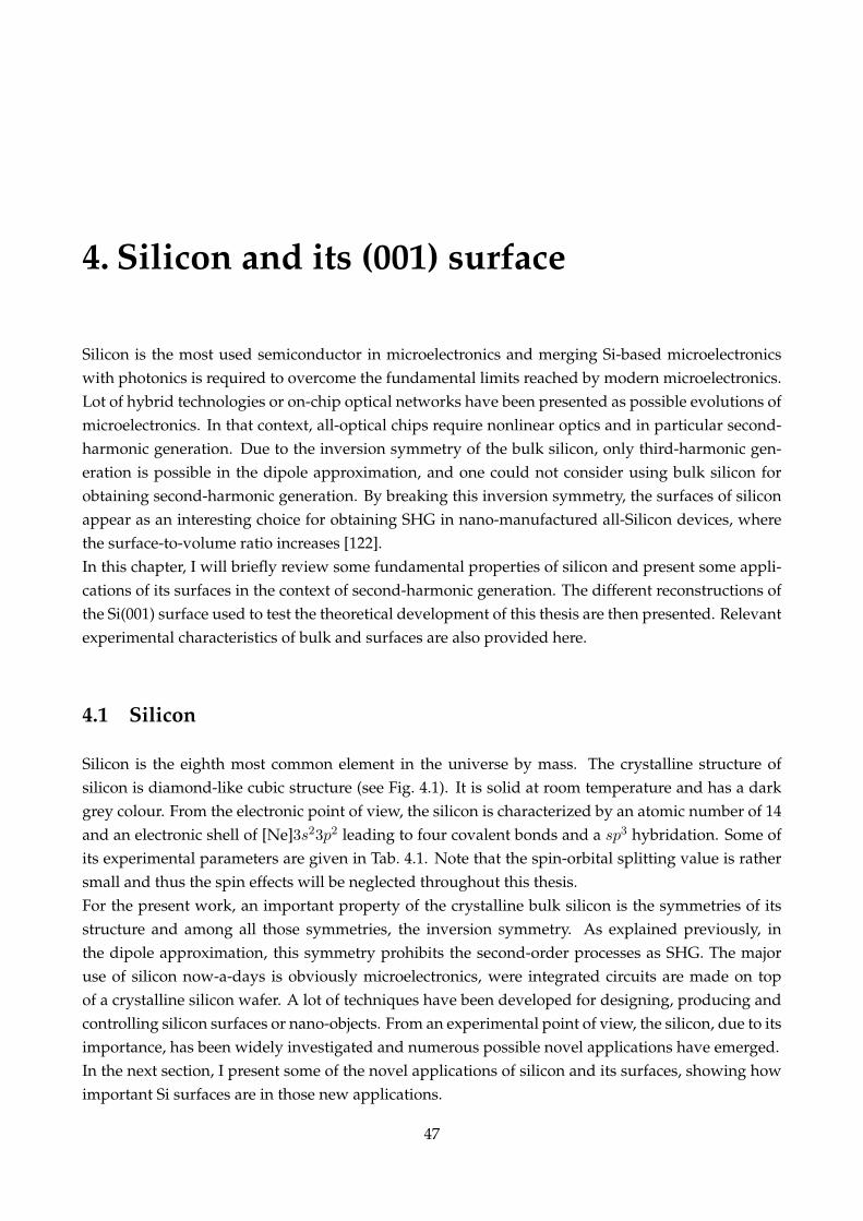
4. Silicon and its (001) surface
Silicon is the most used semiconductor in microelectronics and merging Si-based microelectronicswith photonics is required to overcome the fundamental limits reached by modern microelectronics.Lot of hybrid technologies or on-chip optical networks have been presented as possible evolutions ofmicroelectronics. In that context, all-optical chips require nonlinear optics and in particular second-harmonic generation. Due to the inversion symmetry of the bulk silicon, only third-harmonic gen-eration is possible in the dipole approximation, and one could not consider using bulk silicon forobtaining second-harmonic generation. By breaking this inversion symmetry, the surfaces of siliconappear as an interesting choice for obtaining SHG in nano-manufactured all-Silicon devices, wherethe surface-to-volume ratio increases [122].In this chapter, I will briefly review some fundamental properties of silicon and present some appli-cations of its surfaces in the context of second-harmonic generation. The different reconstructions ofthe Si(001) surface used to test the theoretical development of this thesis are then presented. Relevantexperimental characteristics of bulk and surfaces are also provided here.
4.1 Silicon
Silicon is the eighth most common element in the universe by mass. The crystalline structure ofsilicon is diamond-like cubic structure (see Fig. 4.1). It is solid at room temperature and has a darkgrey colour. From the electronic point of view, the silicon is characterized by an atomic number of 14and an electronic shell of [Ne]3s23p2 leading to four covalent bonds and a sp3 hybridation. Some ofits experimental parameters are given in Tab. 4.1. Note that the spin-orbital splitting value is rathersmall and thus the spin effects will be neglected throughout this thesis.For the present work, an important property of the crystalline bulk silicon is the symmetries of itsstructure and among all those symmetries, the inversion symmetry. As explained previously, inthe dipole approximation, this symmetry prohibits the second-order processes as SHG. The majoruse of silicon now-a-days is obviously microelectronics, were integrated circuits are made on topof a crystalline silicon wafer. A lot of techniques have been developed for designing, producing andcontrolling silicon surfaces or nano-objects. From an experimental point of view, the silicon, due to itsimportance, has been widely investigated and numerous possible novel applications have emerged.In the next section, I present some of the novel applications of silicon and its surfaces, showing howimportant Si surfaces are in those new applications.
47

4.3 The (001) surface of silicon
4.3 The (001) surface of silicon
4.3.1 Surface notations
The different surface reconstructions are named, in Wood notations, by a letter, which can be c orp; standing respectively for centred or primitive. To that letter, one adds two numbers, e.g., p(2×1),where the two numbers indicate how many times the bulk-like unit-cell is repeated along the twoin-plane lattice vectors for obtaining the unit-cell associated to the reconstruction. The more atomsare involved, the bigger the reconstructed unit-cell is. In the case of the p(2×1) reconstruction, the cellis twice longer in the first in-plane direction than in the second. If no letter is present, the reader hasto understand that it as a primitive cell, because the p letter is sometimes omitted. More informationconcerning Wood notations can be found in Ref. [153].
4.3.2 The (001) surface of silicon
In this thesis, I was interested in the some specific silicon surfaces. I have chosen to apply my theoret-ical developments to the (001) surfaces of Silicon for two main reasons. First, most of the electronicdevices are grown on top of wafers with a cubic cleavage on the (001) plane, making this surfaceof main interest from the point of view of industrial applications. Among that industrial applica-tions, one find the micro-fabrication process steps such as the doping or the ion implantation, thephoto-lithographic patterning, the etching, the deposition of various materials and the laser ablation.Second, this surface exhibits simple reconstructions, making possible a study by means of ab initio
methods. By simple reconstructions, one has to understand 1×1 or 2×1 reconstructions, keeping inmind that a 2×1 reconstruction obliges us already to double the number of atoms used for a calcula-tion, increasing the already impressive burden associated with the ab initio calculation of SHG fromsurfaces.
The smallest reconstructions of the clean (001) surfaces are presented in Fig. 4.2. Fig. 4.2 (a) repre-sents the ideal surface, referred also as the bulk-terminated surface. In that bulk-terminated surface,the top-most atoms are missing two neighbouring Si atoms, thus two covalent bounds, leading towhat is called two “dangling” bonds per Si surface atoms. Due to the dangling bonds, this surfaceis not favourable in energy and, depending on the temperature and on the experimental conditions,the atoms reconstruct into different structures as the p(2×1) with asymmetric dimers (Fig. 4.2(b)), thep(2×2) with alternated dimers (Fig. 4.2(c)) or the c(4×2) structure (Fig. 4.2(d)). A careful study of theenergy associated with these different reconstructions can be found in Ref. [154]. As a summary, thep(2×1) is the most favourable structure at room temperature, whereas the c(4×2) is the most stablereconstruction at low temperature [153]. The phase transition p(2×1)→ c(4×2) takes place around200K [155]. Due to its simplicity and the fact that at room temperature, the p(2×1) surface is themost stable, I have decided to choose this surface reconstruction for representing the clean surface ofSi(001). Details concerning the asymmetric dimers are given in the following section.Finally, it is important to mention that the Si(001) surface exhibits vicinal surfaces, which have beenextensively studied [156–158]. Such surfaces are Si(001) surfaces with a small miscut (of few degrees)towards the crystallographic directions [110] or [111]. Nevertheless these surfaces require a study in
49

Chapter 4. Silicon and its (001) surface
Fig. 4.2: Top view of different possible reconstructions of the Si(001) surface. (a) Ideal surface. (b)The p(2×1) reconstruction with asymmetric dimers. (c) The p(2×2) reconstruction with alternatedasymmetric dimers. (d) The c(4×2) reconstruction. Details concerning these surfaces are given in thetext. The top-most atoms are displayed in white. Red dashed lines correspond to the smallest cellneeded for mapping the entire surface.
themselves and will not be investigated in this present thesis.In next section, the reconstructions used latter in this thesis are presented more in details.
4.4 Geometries and reconstructions
During this thesis, I have investigated three specific reconstructions of the silicon surface, along thecleavage direction (001). Most of the effort has been devoted to the clean Si(001)2×1 surface. Twoother surfaces, obtained by the adsorption of hydrogen, namely the monohydride and the dihydridesurfaces, have been also investigated and are presented in that section.
4.4.1 Asymmetric dimers vs. Symmetric dimers
The 2×1 reconstruction of the clean Si(001) surface is known to be the most stable reconstructionat room temperature [153]. This reconstruction arises from the dimerization of Si top-most surfaceatoms, halving the number of dangling bonds (see Fig. 4.3(a) and (b)). It has been proposed twomodels for the dimers, the symmetric dimers model where the dimers are parallel to the surface andthe asymmetric dimers model where dimers are buckled. The idea of the asymmetric dimers origi-nates from Chadi [159], who found from tight-binding calculations that the Si(001)2×1 surface withsymmetric dimers was metallic, in disagreement with experimental results published the same year,
50

4.4 Geometries and reconstructions
Fig. 4.3: (a) Atomic Force Microscope (AFM) image of the clean Si(001)2×1 surface, from Ref. [162].(b) Schematic view of the Si(001)2×1 surface. Picture from NIST Surface Structure Database. (c)Evolution of opinions about the structure of clean Si(001) surface, taken from Ref. [163]. Symmetricdimers dominates between the first observation of mostly symmetric dimers at room temperature(1985) and first observation of mostly buckled dimers at low temperature (1992). In the upper panel,the value of the buckling angle obtained from theoretical and experimental studies is reported, witha clear correlation. The middle panel report the support for each model, measured by the numberof published papers. The theoretical and experimental preference (lower panel) is measured by thedifference between the number of papers supporting either model.
obtained by angle-resolved photo-emission spectroscopy (ARPES) [160].From that seminal paper, lot of effort has been devoted to investigate the character of the dimers ofthat surface. As a summary, one can keep in mind that the asymmetric dimers are found to be morefavourable in total energy by 0.1 eV per unit cell [161], and that they give the correct semiconductingcharacter of the surface.One can think that the metallic character obtained by tight-binding or LDA calculations can bechanged by a GW correction, which opens the underestimated band-gap of LDA calculations, butit has been shown in Ref. [161] that the GW band-structure obtained assuming symmetric dimersis also metallic. As a conclusion, one can see on Fig. 4.3(c) that it is now well admitted from boththeoretical and experimental communities that dimers of the Si(001)2×1 are asymmetric.
Fig. 4.4: Side view of theasymmetric dimer. dl isthe dimer length and dbthe dimer buckling. θb isthe buckling angle.
The clean Si(001) surface used in this thesis corresponds to theSi(001)2×1 surface with asymmetric dimers. Its point group is m and thecorresponding space group is p1m1. The dimers are along the [110] crys-tallographic direction (x-axis) and the dimer rows are along the [110] di-rection (y-axis). Thus the surface is invariant under only one symmetry,which is y → −y. The dimers are characterized by two values, which arethe dimer-bond length and the dimer buckling, as reported in Fig. 4.4. Al-ternatively to the buckling value, the dimers can be characterized by thebuckling angle. The values of the dimer bond-length and buckling angle
51
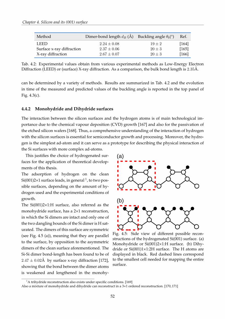
Chapter 4. Silicon and its (001) surface
Method Dimer-bond length dB (Å) Buckling angle θb(°) Ref.
LEED 2.24± 0.08 19± 2 [164]Surface x-ray diffraction 2.37± 0.06 20± 3 [165]X-ray diffraction 2.67± 0.07 20± 3 [166]
Tab. 4.2: Experimental values obtain from various experimental methods as Low-Energy ElectronDiffraction (LEED) or (surface) X-ray diffraction. As a comparison, the bulk bond length is 2.35Å.
can be determined by a variety of methods. Results are summarized in Tab. 4.2 and the evolutionin time of the measured and predicted values of the buckling angle is reported in the top panel ofFig. 4.3(c).
4.4.2 Monohydride and Dihydride surfaces
The interaction between the silicon surfaces and the hydrogen atoms is of main technological im-portance due to the chemical vapour deposition (CVD) growth [167] and also for the passivation ofthe etched silicon wafers [168]. Thus, a comprehensive understanding of the interaction of hydrogenwith the silicon surfaces is essential for semiconductor growth and processing. Moreover, the hydro-gen is the simplest ad-atom and it can serve as a prototype for describing the physical interaction ofthe Si surfaces with more complex ad-atoms.
Fig. 4.5: Side view of different possible recon-structions of the hydrogenated Si(001) surface. (a)Monohydride or Si(001)2×1:H surface. (b) Dihy-dride or Si(001)1×1:2H surface. The H atoms aredisplayed in black. Red dashed lines correspondto the smallest cell needed for mapping the entiresurface.
This justifies the choice of hydrogenated sur-faces for the application of theoretical develop-ments of this thesis.The adsorption of hydrogen on the cleanSi(001)2×1 surface leads, in general 1, to two pos-sible surfaces, depending on the amount of hy-drogen used and the experimental conditions ofgrowth.The Si(001)2×1:H surface, also referred as themonohydride surface, has a 2×1 reconstruction,in which the Si dimers are intact and only one ofthe two dangling bounds of the Si dimer is H sat-urated. The dimers of this surface are symmetric(see Fig. 4.5 (a)), meaning that they are parallelto the surface, by opposition to the asymmetricdimers of the clean surface aforementioned. TheSi-Si dimer bond-length has been found to be of2.47 ± 0.02Å by surface x-ray diffraction [172],showing that the bond between the dimer atomsis weakened and lengthened in the monohy-
1A trihydride reconstruction also exists under specific conditions. [169]Also a mixture of monohydride and dihydride can reconstruct in a 3×1 ordered reconstruction. [170, 171]
52

4.4 Geometries and reconstructions
dride structure, as we compare to the clean surface using similar experimental techniques. Thissurface can be obtained experimentally by adsorption of hydrogen at high temperature, where the2×1 organisation is preserved [34, 169]. This surface is also referenced as the surface with a coverageof 1 mono-layer (ML) of hydrogen.The space group of this surface is p2mm. The dimers are chosen to be along the same direction as theclean surface. As the dimer are symmetric, the system is also invariant under the symmetry x→ −x.
The Si(001)1×1:2H surface (see Fig. 4.5(b)), also referred as the dihydride surface, is obtained bysaturating all the dangling bonds of the Si(001) surface with hydrogen atoms and can be obtainedexperimentally if enough H (2ML) is added to the surface, so breaking dimers [34, 169]. Thus thissurface preserves the bulk symmetries and the hydrogenated surface so obtained is an ideally bulk-terminated surface where hydrogen atoms saturate all the dangling bounds. The Si-H bond lengthis found experimentally to be 1.48Å, from the SiH4 molecule [173]. By opposition to the two othersurfaces, this surface has a 1×1 reconstruction, leading to different symmetries for the χ(2) tensor;due to its space group p4mm.
53

Part II
Microscopic theory of second-harmonicgeneration from crystal surfaces
55


5. Microscopic theory ofsurface second-harmonic generation
Fig. 5.1: From the slabgeometry (a) to the semi-infinite medium (b).
Second-harmonic generation (SHG) is considered to be a versatile tool tostudy many kinds of surfaces [65–67], interfaces [68, 69] and nanostruc-tures [174–176]. The theoretical description of the phenomenon is wellestablished for bulk materials and interfaces and gives reliable results[29, 41, 177, 178], but a rigorous theoretical description of the SHG fromsurfaces is still missing. This can be easily understood because it is notpossible to compute directly the surface second-harmonic generation bythe usual ab initio approaches for surfaces. This is that particular problemI want to address in this chapter.
The best model that one can imagine for representing a surface is asemi-infinite crystal that fills half of the space, say for instance z>0, withits surface parallel to the x-y plane; as sketched in Fig. 5.1(b). Unfortu-nately, it is difficult, if not impossible, to treat numerically a semi-infinite crystal. The standardapproach, which is the one adopted in this thesis, consists in replacing the semi-infinite medium bya finite slab of matter, i.e., a thin film, in order to mimic the semi-infinite crystal [119], see Fig. 5.1(a).This slab is periodic in the plane, as the surface that we want to treat. In the direction perpendicularto the plane of the surface, the slab, together with some vacuum, is repeated, in order to fill all thespace. This approach is called the super-cell approach. It has been successfully applied to surfaces,for computing linear differential spectroscopies, e.g., the reflectance anisotropy; leading to quantita-tive results [179–181].Describing a surface by a slab of thickness 2L is a perfectly valid approach for representing a semi-infinite crystal, under two conditions. i) The spectra originating from one half of the slab can beobtained, independently of the other half of the slab. This means that the presence of the back sur-face does not affect the optical response of the front surface, and vice versa. ii) One is able to take thelimit L → ∞, as sketched in Fig. 5.1. This last point is easily done in practice, by increasing L up tothe point where the surface spectroscopical quantities are converged.1
In the case of linear optics, the optical response of the half-slab is obtained by dividing by two thefull slab response, at least within the IPA [182].
1Surface spectroscopical quantities means there is no contribution from the bulk part. Linear differential spectroscopiesand SHG from centro-symmetric crystal surfaces are valid surface spectroscopical quantities in this context.
57

Chapter 5. Microscopic theory of surface second-harmonic generation
Problems arise when applying this technique to the calculation of the second-harmonic generation.The slab of matter being surrounded by vacuum, it exhibits two surfaces. If the slab is symmetric,as exemplified in Fig. 5.2, the full slab exhibits artificial inversion symmetry and does not yield anySHG signal.
Fig. 5.2: A symmetricslab exhibits an artificialcentro-symmetry
If the slab is non-symmetric, the SHG computed is non-zero, but thespectra so obtained results from the destructive interferences between thetwo surface contributions.2 It can be shown that there is no general com-bination of slabs and surfaces that allows us to obtain the contributionarising from a single surface, independently of the other one.In this chapter, I present how it is possible to obtain the second-harmonicgeneration spectra from half of the slab, in super-cell geometry. First Ipresent the theory behind the extraction procedure, which gives access tothe contribution of a single surface. Then a relevant test-case is presented,showing the consistency of the method. In Sec. 5.2, the accuracy of the ex-traction and potential sources of errors are discussed. Finally, the spatialconstruction of the spectra is analysed.In all this chapter, the second-order surface susceptibility is considered, atthe level of the Independent-Particle Approximation (IPA). The local-fieldeffects are treated later, in Chap. 7.
5.1 Extracting the surface second-harmonic generation spectra
In this chapter, we consider the surface of a centrosymmetric crystal, such as silicon. In this case, onlythe surface region contributes to the signal. The second-harmonic generation from half of the slabreduces to only the surface region. I thus refer to the extracted spectra equally as the surface spectraor the half-slab spectra.The first atomistic calculations of second-harmonic generation from a surface have been performedby L. Reining et al. [183]. In this paper, authors assumed that the electric field of the incident light hasa z dependence denoted C(z) and they replaced some matrix elements of the momentum, defined asp = i[H, r], by matrix elements of the modified momentum
P =C(z)p+ pC(z)
2. (5.1)
Then, they computed the probability of SHG in the velocity gauge by modifying the interaction be-tween the electrons and the incident photons, and so introducing the modified momentum matrixelements defined by Eq. (5.1). Two matrix elements are thus modified in this approach, correspond-ing to the two impinging photons involved in SHG process.Later, some authors (see Ref. [135–141]) have applied a similar technique, i.e., using the same modi-fied momentum, but for computing the IPA second-order susceptibility χ(2)
0 (and no more the proba-bility of SHG). They adopted a different approach, modifying only one matrix element, arguing that
2This is a major difference with linear optical properties where the contributions originating from the two surfacesinterfere positively.
58
5.1 Extracting the surface second-harmonic generation spectra
the field corresponding to emitted photon must be modified (or equivalently to the dielectric polar-ization) and not the field corresponding to the two impinging photons. However the literature doesnot provide us with any reason for choosing one of those two methods nor a proof of one of thosemethods.In this section, I will prove the second method to be the correct way for extracting the half-slab spec-tra; without using any phenomenological argument such as the emitted or impinging photons.The microscopic second-order susceptibility is given, in the velocity gauge and within the independent-particle approximation by [184]
χ(2)0,αβγ(ω, ω) =
i
2V ω3
∑
n,n′,n′′
BZ∑
k
〈nk|pα|n′k〉(
〈n′k|pβ |n′′k〉〈n′′k|pγ |nk〉+ 〈n′k|pγ |n′′k〉〈n′′k|pβ |nk〉)
(En,k − En′,k + 2ω + 2iη)
×[
fnn′′
(En,k − En′′,k + ω + iη)+
fn′n′′
(En′′,k − En′,k + ω + iη)
]
,
(5.2)where V is the volume of the crystal, fnn′′ = fn − fn′′ with fn3 and En,k being respectively the Fermioccupation number for the Bloch state n at the point k in the BZ, and its energy. The frequency of theimpinging light is ω, and η is a small imaginary number that turns on adiabatically the electric field.Here, α, β and γ are Cartesian coordinates.Thereby, according to all the previous references except Ref. [183], the surface second-order suscepti-bility should be computed using the formula
χ(2)Cz10,αβγ (ω, ω) =
i
2V ω3
∑
n,n′,n′′
BZ∑
k
〈nk|Pα|n′k〉(
〈n′k|pβ |n′′k〉〈n′′k|pγ |nk〉+ 〈n′k|pγ |n′′k〉〈n′′k|pβ |nk〉)
(En,k − En′,k + 2ω + 2iη)
×[
fnn′′
(En,k − En′′,k + ω + iη)+
fn′n′′
(En′′,k − En′,k + ω + iη)
]
,
(5.3)where P is defined by Eq. (5.1).Let us call this modification Cz1, because only one matrix element is modified in this formula. Onthe other hand, the susceptibility is obtained according to Ref. [183] thanks to the formula
χ(2)Cz20,αβγ (ω, ω) =
i
2V ω3
∑
n,n′,n′′
BZ∑
k
〈nk|pα|n′k〉(
〈n′k|Pβ |n′′k〉〈n′′k|Pγ |nk〉+ 〈n′k|Pγ |n′′k〉〈n′′k|Pβ |nk〉)
(En,k − En′,k + 2ω + 2iη)
×[
fnn′′
(En,k − En′′,k + ω + iη)+
fn′n′′
(En′′,k − En′,k + ω + iη)
]
.
(5.4)This modification will be referred as Cz2, because two momentum matrix elements are modified.Notice that the key point for the extraction of the spectra in both approaches is based on the modifiedmomentum P .With those two unproven methods, the literature does not really provide the reader with a rigorous
3The system is a cold semiconductor with filled band, at T=0K. The occupation numbers are thus independent of themomentum k.
59

Chapter 5. Microscopic theory of surface second-harmonic generation
theoretical description of the second-harmonic generation from surface. Some questions have to beaddressed. Is one of these two methods correct? Is there a different way to extract the spectra fromhalf of the slab? If one of these two approaches is correct, what justifies the choice of Eq. (5.1) as aexpression for P? Answering to these different questions is the aim of this chapter and in particularof this section.Using the argument of the gauge invariance, I will first prove that the modification denoted Cz1 al-lows the gauge invariant whereas this is not the case for other possible modifications of the formula.Then, in section 5.1.2, I will derive the Cz1 formula and prove that the expression of the modifiedmomentum can be rigorously obtained, e.g., from the density-matrix formalism and the perturbationtheory; by integrating the microscopic current over the region of the slab limited by the aforemen-tioned C(z) function.
5.1.1 Gauge invariance
The gauge invariance is an intrinsic property of the response functions [44]. This implies some prop-erties on the χ(2)
0 tensor. Here I will focus on one necessary condition to be gauge invariant, which isthe non-divergence of the χ(2)
0 tensor as ω goes to zero.Expressed in the velocity gauge, as in Eq. 5.2, there is an apparent divergence as the frequency ω goesto zero. However, Sipe and co-workers proved in Ref. [185] that the formula can be expressed in anon-divergent form, in the length gauge, and that all the divergent terms vanish.The natural property of the tensor to be non-divergent must be fulfilled in an exact description ofmicroscopic surface second-harmonic generation. Therefore, the modified formula allowing us toextract half of the slab response, must respect this property. As we will see, this is not the case forall the possible modifications of the formula, and only the Cz1 formula fulfils the non-divergencecondition, and therefore allows the gauge invariance.The Sipe and co-workers gauge transformation is based on the following expansion
1
ω3(Enn′(k) + 2ω)
[
fnn′′
(Enn′′(k) + ω)+
fn′n′′
(En′′n′(k) + ω)
]
=Aω3
+Bω2
+Cω+ F(ω), (5.5)
where
A =1
Enn′(k)
[
fnn′′
Enn′′(k)+
fn′n′′
En′′n′(k)
]
, (5.6a)
B =fnn′′
Enn′(k)Enn′′(k)
[
2
En′n(k)+
1
En′′n(k)
]
+fn′n′′
Enn′(k)En′′n′(k)
[
2
En′n(k)+
1
En′n′′(k)
]
, (5.6b)
C =fnn′′
Enn′(k)Enn′′(k)
[
4
En′n(k)2+
2
En′n(k)En′′n(k)+
1
En′′n(k)2
]
+fn′n′′
Enn′(k)En′′n′(k)
[
4
En′n(k)2+
2
En′n(k)En′n′′(k)+
1
En′n′′(k)2
]
, (5.6c)
F(ω) =16
E3n′n(k)(Enn′(k) + 2ω)
[
fnn′′
(En′n(k)− 2En′′n(k))+
fn′n′′
(En′n(k)− 2En′n′′(k))
]
60

5.1 Extracting the surface second-harmonic generation spectra
+fnn′′
E3n′′n(k)(2En′′n(k)− En′n(k))(Enn′′(k) + ω)
+fn′n′′
E3n′n′′(k)(2En′n′′(k)− En′n(k))(En′′n′(k) + ω)
,
(5.6d)
where Enn′(k) = En,k − En′,k.To be non-divergent, the terms associated with A, B and C must be zero.Here, I do not assume any explicit expression for P and I only assume that p and P behave similarlyunder time-reversal symmetry and thus that 〈n,−k|P |n′,−k〉 = −〈n,k|P |n′,k〉.
Cz1 modification
Following Ref. [185], it is straightforward to show that the terms associated with A and C are zero,invoking the time-reversal symmetry. In order to prove that the term associated with B is zero, wemust define the second-rank tensor
↔T (k) =
∑
n,n′ /∈Dn
fnn′〈n,k|P |n′,k〉〈n′,k|p|n,k〉
E2n′n(k)
.
Using the k.p perturbation theory, and after some algebra, we obtain
1
2
(
∂Tαβ
∂kγ+∂Tαγ
∂kβ
)
=∑
n,n′ /∈Dn
fnn′∆αnn′(k)
〈n,k|pβ |n′,k〉〈n′,k|pγ |n,k〉
E2n′n(k)
−∑
n,n′
(
3fnn′〈n,k|Pα|n′,k〉〈n′,k|pβ |n,k〉∆γn′n(k)
E3n′n(k)
+fnn′〈n,k|C(z)δαγ |n′,k〉〈n′,k|pβ |n,k〉
E2n′n(k)
)
−∑
n,n′,n′′
n′ /∈Dn
n′′ /∈DnDn′
βn,n′,n′′(k)〈n,k|Pα|n′,k〉〈n′,k|pβ |n′′,k〉〈n′′,k|pγ |n,k〉,
(5.7)
with ∆αnn′(k) = 〈n,k|Pα|n,k〉 − 〈n′,k|Pα|n′,k〉, and
〈n,k|pβ |n′,k〉〈n′,k|pγ |n,k〉
=1
2
(
〈n,k|pβ |n′,k〉〈n′,k|pγ |n,k〉+ 〈n,k|pγ |n′,k〉〈n′,k|pβ |n,k〉)
.
In order to obtain Eq.(5.7), we have used the following sum-rule
∂
∂kγ〈n,k|Pα|n′,k〉 = i
∑
m/∈DnDn′
[
〈n,k|rγ |m,k〉〈m,kPα|n′,k〉 − 〈n,k|Pα|m,k〉〈m,k|rγ |n′,k〉]
−〈n,k|C(z)δαγ |n′,k〉+ i〈n,k|rγ |n′,k〉∆αn′n, (5.8)
that can be derived from the k.p perturbation theory. Here Dn are all the possible degenerate n-states.Using the time-reversal symmetry, we obtain that
1
2
(
∂Tαβ
∂kγ+∂Tαγ
∂kβ
)
= −∑
n,n′,n′′
n′ /∈Dn
n′′ /∈DnDn′
βn,n′,n′′(k)〈n,k|Pα|n′,k〉〈n′,k|pβ |n′′,k〉〈n′′,k|pγ |n,k〉. (5.9)
61
Chapter 5. Microscopic theory of surface second-harmonic generation
Using the fact that↔T (k) is a periodic function throughout the BZ, its integral over the full BZ is zero.
The βn,n′,n′′(k) term corresponds to the B term of Eq. (5.6b); which is integrated over the full BZ. Wethus prove that the term associated with B, in the case of the formula Cz1, is zero which is a necessarycondition for the formula Cz1 to be gauge invariant.
Cz2 modification
Similarly to the previous case, the terms associated to A and C are zero from time-reversal symmetry.The term associated to B contains two modified matrix elements. The sum-rule Eq. (5.8) yields onlyone modified momentum matrix element on the right-hand side. In order to allow the gauge invari-ance, one must define a second-rank tensor, and takes its derivative. The only possible choice forobtaining two modified momentum matrix elements from the derivative of a second-order tensor, isto define the following tensor
↔T (k) =
∑
n,n 6=n′fnn′
〈n,k|P |n′,k〉〈n′,k|P |n,k〉E2
n′n(k). (5.10)
More precisely, due to the structure of B, only the specific combination of derivative of that tensor12
(
∂T bc
∂ka + ∂T cb
∂ka
)
would give the correct coordinates associated with the modified momentum matrixelements. Any other combination does not yield the correct coordinates associated with P . Unfor-tunately, it is not possible to recover the expected B term from this expression. The conclusion is the
formula Cz2 is not gauge invariant, due to the fact that B term is non-vanishing.
Other possible modifications
We have, up to now, considered only Cz1 and Cz2 as possible modifications for the expression ofthe second-order susceptibility tensor. But is there any other possible modifications? One can thinkfor instance to modify one matrix element but not the first one, or to modify two matrix elementsbut not the two last one. First, this is meaningless because this breaks the intrinsic permutation ruleof the indices of the χ(2)
0 tensor, χ(2)0,αβγ = χ
(2)0,αγβ . Second, in each cases, applying the time-reversal
symmetry to the A and C terms does not make them vanish.The last possible option could be to modify all matrix elements. In that case, due to the sum-ruleEq. (5.8), the B term will not be zero, because any derivative of a second-order tensor will leave, atleast, one unmodified momentum matrix element.
Conclusion
To conclude, I have proven that the only modified expression of the microscopic second-order sus-ceptibility tensor, which includes the cut-function C(z) while allowing gauge invariance, is the Cz1
62

5.1 Extracting the surface second-harmonic generation spectra
modified quantity; which will now be denoted χ(2)S0 , and which is given by
χ(2)S0,αβγ(ω, ω) =
i
2V ω3
∑
n,n′,n′′
BZ∑
k
〈nk|Pα|n′k〉(
〈n′k|pβ |n′′k〉〈n′′k|pγ |nk〉+ 〈n′k|pγ |n′′k〉〈n′′k|pβ |nk〉)
(En,k − En′,k + 2ω + 2iη)
×[
fnn′′
(En,k − En′′,k + ω + iη)+
fn′n′′
(En′′,k − En′,k + ω + iη)
]
Nevertheless, at this stage, I do not have proven that this modified formula gives the correctsecond-harmonic generation spectra. Moreover, the analytical expression of the modified momen-tum has still not been given. The only thing that I have proven at this point is that gauge invarianceimposes only one way to modify the formula. The interesting point is that this choice corresponds tothe choice of the majority of authors in the literature. I will now show the expression of P .
5.1.2 Density-matrix formalism and perturbation theory
In Ref. [139], Mendoza et al. derived from a microscopic approach the modification Cz1 for thelinear optical properties; by integrating the polarization (and therefore the microscopic current) overthe surface region. Here I briefly reproduce their derivation for the linear case and I extend it to thecase of the second-harmonic generation. The potential is assumed here to be local. The specificitiesrelated to non-local operators are treated in next chapter.For a system perturbed by an external electric field, Sipe et al. [186] have shown, from perturbationtheory, that the corrections to density matrix due to the perturbing field, denoted here cmn(k, t), aregiven at first- and second-order in the perturbing electric field, by
c(1)mn(k, t) =
∫
dω∑
β
fnmrβmn(k)
(Emn(k)− ω − iη)EP
β (ω)e−i(ω+iη)t (5.11a)
c(2)mn(k, t) =i
4
∫
dω1dω2
∑
βγ
1
(Emn(k)− (ω1 + ω2 + 2iη))
[
fnmrβmn;γ(k)
(Emn(k)− ω1 − iη)− fnmr
βmn(k)∆
γmn(k)
(Emn(k)− ω1 − iη)2
−i∑
p
( fnprγmp(k)r
βpn(k)
(Epn(k)− ω1 − iη)− fpmr
βmp(k)r
γpn(k)
(Emp(k)− ω1 − iη)
)
+ (βγ12 ⇔ γβ21)
]
EPβ (ω1)E
Pγ (ω2)e
−i(ω1+ω2+2iη)t
(5.11b)
where EP (ω) =∫
dtEP (t)exp(iωt), EP being the perturbing field, see Chap. 1.Here, Emn(k) = Em,k − En,k are energy differences between the bands m and n for a momentum k
in the BZ, ∆γmn is defined as ∆γ
mn(k) = pγmm(k)− pγnn(k) and rβmn;γ is given by
rβmn;γ(k) =−[rβmn(k)∆
γmn(k) + rγmn(k)∆
βmn(k)]
Emn(k)− i∑
p
Emp(k)rβmp(k)r
γpn(k)− Epn(k)r
γmp(k)r
βpn(k)
Emn(k).
(5.12)Even if the expression (5.11b) is general for all the second-order phenomena, I will restrict myself tothe case of second-harmonic generation.Following Ref. [139], we write the mean value of the microscopic current density integrated over the
63

Chapter 5. Microscopic theory of surface second-harmonic generation
full BZ 4
< j(1)(r, t) > =
∫
d3k
8π3
∑
mn
c(1)mn(k, t)jnm(k; r), (5.13a)
< j(2)(r, t) > =
∫
d3k
8π3
∑
mn
c(2)mn(k, t)jnm(k; r), (5.13b)
where jnm(k; r) is a matrix element of the microscopic current operator given by [187]
jnm(k; r) =−i2[ψ∗
nk(r)∇ψmk(r)− ψmk(r)∇ψ∗nk(r)]. (5.14)
Rather than integrating over the full slab, we integrate over a part of the slab, defined by C(z). Thesurface microscopic induced current density JS
ind is given at the i-th order by
< J(i)Sind (t) >=
∫
d3rC(z) < j(i)(r, t) >=
∫
d3k
8π3
∑
mn
c(i)mn(k, t)
∫
d3rC(z)jnm(k; r). (5.15)
We now compute the last integral in Eqs. (5.15).
∫
d3rC(z)jnm(k; r) =1
2
∫
d3rC(z)[ψ∗nk(r)(−i∇)ψmk(r) + ψmk(r)(i∇)ψ∗
nk(r)]
=
∫
d3rψ∗nk(r)
C(z)p+ pC(z)2
ψmk(r)
= Pnm(k), (5.16)
where p = −i∇.Here an integration by part is performed on the second term of the right-hand side of the first line.Notice that we obtain the expression of a matrix element of the modified momentum mentionedbefore.The next step consists in linking explicitly c(1)mn and c
(2)mn, given by expressions (5.11a) and (5.11b), to
the linear and second-order susceptibilities.
First-order response
Using Eq.(5.16) and Eq.(5.15), we obtain5
< J(1)S,αind (t) >=
∫
dω∑
β
∫
d3k
8π3
∑
mn
fnmPαnm(k)pβmn(k)
Emn(k) (Emn(k)− ω − iη)EP
β (ω)e−i(ω+iη)t. (5.17)
4At this point of the derivation, one must not replace the integral over the Brillouin zone by a sum because an integrationby part will be performed later.
5Position matrix elements are linked to the momentum matrix elements by the relation
rnm(k) =pnm
iEnm(k), n /∈ Dm,
where Dm are all the possible degenerate m-states. The occupation numbers prevent from having n ∈ Dm.
64

5.1 Extracting the surface second-harmonic generation spectra
We now use the following definition, where χ(1)S0 is the first-order surface susceptibility, linking the
surface polarization at first order to the electric field.6
< J(1)S,αind (t) >= −i
∫
dω∑
β
(ω + iη)χ(1)S0,αβ(ω)E
Pβ (ω)e
−i(ω+iη)t.
After simple algebra, one obtains that
χ(1)S0,αβ(ω) =
1
V
∑
mn
BZ∑
k
fnm〈n,k|Pα|m,k〉〈m,k|pβ |n,k〉E2
mn(k) (Emn(k)− ω − iη), (5.18)
where we replaced the integral over the BZ by a sum. We obtain exactly the same formula as in[188], except that the first momentum matrix element is replaced by a matrix element of the modifiedmomentum (5.1).Thus we showed that computing the first-order microscopic susceptibility for a surface yield the Cz1formula Eq. (5.3). Moreover, the expression of the modification P , given by Eq.(5.1), is obtainedanalytically.
Second-harmonic generation
The case of SHG is more difficult to tackle.Combining Eq. (5.16) and Eq. (5.15), and identifying to the surface susceptibility defined by
< J(2)Sind,α(t) >= −i
∫
dω∑
βγ
(ω + iη)χ(2)S0,αβγ(ω, ω)E
Pβ (ω)E
Pγ (ω)e
−2i(ω+iη)t, (5.19)
we obtain that
χ(2)S0,αβγ(ω, ω) =
−i(ω + iη)
∫
d3k
8π3
∑
mn
1
(Emn(k)− 2ω − 2iη)
[
fnmPαnm(k)
[
pbmn(k)∆cmn(k) + pcmn(k)∆
bmn(k)
]
(Emn(k)− ω)E2mn(k)
+∑
p
fnmPαnm(k)
[
Emp(k)pβmp(k)pcpn(k)− Epn(k)p
cmp(k)p
bpn(k)
]
Emp(k)Epn(k)Emn(k)(Emn(k)− ω − iη)+fnmPα
nm(k)pβmn(k)∆cmn(k)
Emn(k)(Emn(k)− ω − iη)2
+∑
p
( fnpPαnm(k)pcmp(k)p
bpn(k)
Emp(k)Epn(k)(Epn(k)− ω − iη)−
fpmPαnm(k)pbmp(k)p
cpn(k)
Emp(k)Epn(k)(Emp(k)− ω − iη)
)
+ (βγ ⇔ γβ)
]
.
(5.20)This expression is divergent as 1
(ω+iη) , but after some tedious algebra, we obtain a non-divergentformula. The derivation proceeds as follow. The following term
A =−i
2(ω + iη)
∫
d3k
8π3
∑
mn
fnmPanm(k)pbmn(k)∆
cmn(k)
ωmn(k)(ωmn(k)− 2ω − 2iη)(ωmn(k)− ω − iη)2,
is not satisfactory because it contains a term with (ωmn(k)−ω−iη)−2. In order to overcome this term,we expand A into partial fraction and we use a relation given by Sipe and co-workers in Ref. [186]
6The total electric field and the perturbing electric field are equals in the independent-particle approximation.
65

Chapter 5. Microscopic theory of surface second-harmonic generation
for any function g∂g(ωmn)
∂ka=∂ωmn
∂ka∂g(ωmn)
∂ωmn= ∆a
mn
∂g(ωmn)
∂ωmn.
Then after performing integration by parts, all the terms are factorized and simplified using time-reversal symmetry. The 1
(ω+iη) divergence vanishes naturally when applying the time-reversal sym-metry on the remaining expression. For convenience, we split this expression into two contributions,one giving the two-bands contribution, where only two bands are involved and a second one, givingthe contribution which involves three bands.
χ(2)S0,αβγ(ω, ω) = χ3bnd
αβγ (ω) + χ2bndαβγ (ω), (5.21)
with
χ3bndαβγ (ω) =
i
2V
∑
nmp
BZ∑
k
〈n,k|Pα|m,k〉(
〈m,k|pβ |p,k〉〈p,k|pγ |n,k〉+ 〈m,k|pγ |p,k〉〈p,k|pβ |n,k〉)
(2Epn(k)− Emn(k))
×[
16fnmE3
mn(k)(Emn(k)− 2ω − 2iη)+
fpnE3
pn(k)(Epn(k)− ω − iη)+
fmp
E3pm(k)(Emp(k)− ω − iη)
]
,
(5.22a)
χ2bndαβγ (ω) =
i
V
∑
nm
BZ∑
k
fnm〈n,k|Pα|m,k〉(
〈m,k|pβ |n,k〉〈m,k|∆γ |n,k〉+ 〈m,k|pγ |n,k〉〈m,k|∆β |n,k〉)
ω4mn(k)
×[
8
(Emn(k)− 2ω − 2iη)− 1
2(Emn(k)− ω − iη)
]
. (5.22b)
We have replaced integral by a sum over the full BZ. We obtain a formula for χ(2)S0 expressed in
the length gauge similar to the expressions of χ(2)0 that one can find in the literature, e.g., Ref. [189];
except that the momentum matrix element associated with the Cartesian coordinate α of the polar-ization has been replaced here by a modified momentum matrix element.Thereby we have derived explicitly the Cz1 expression, without any approximation on the second-order susceptibility. As in the case of linear optical properties, we recovered the analytical expressionof P as given by Eq.(5.1); proving thus the correctness of the approach assumed by authors in litera-ture.Together with the previous result, we have established a rigorous derivation of the extraction of thesurface second-harmonic generation. We have proven that it exists an unique way to modify the ex-pression of the χ(2)
0 tensor. Then we have proven that integrating over a region of the system definedby a cut-function C(z), instead of the entire system, leads to modified momentum P of the literature.Next section is dedicated to the numerical validation of this approach.
5.1.3 Tight-binding results - Numerical Validation
Tight-binding
The tight-binding (TB) method, using a sp3d5s∗ basis-set, [190, 191] gives reliable results for the elec-tronic structure and the optical properties of solids. As the qualitative effects of the extraction of
66
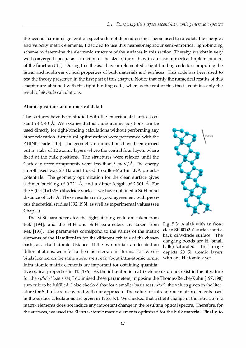
5.1 Extracting the surface second-harmonic generation spectra
the second-harmonic generation spectra do not depend on the scheme used to calculate the energiesand velocity matrix elements, I decided to use this nearest-neighbour semi-empirical tight-bindingscheme to determine the electronic structure of the surfaces in this section. Thereby, we obtain verywell converged spectra as a function of the size of the slab, with an easy numerical implementationof the function C(z). During this thesis, I have implemented a tight-binding code for computing thelinear and nonlinear optical properties of bulk materials and surfaces. This code has been used totest the theory presented in the first part of this chapter. Notice that only the numerical results of thischapter are obtained with this tight-binding code, whereas the rest of this thesis contains only theresult of ab initio calculations.
Atomic positions and numerical details
Fig. 5.3: A slab with an frontclean Si(001)2×1 surface and aback dihydride surface. Thedangling bonds are H (smallballs) saturated. This imagedepicts 20 Si atomic layerswith one H atomic layer.
The surfaces have been studied with the experimental lattice con-stant of 5.43 Å. We assume that ab initio atomic positions can beused directly for tight-binding calculations without performing anyother relaxation. Structural optimizations were performed with theABINIT code [115]. The geometry optimizations have been carriedout in slabs of 12 atomic layers where the central four layers wherefixed at the bulk positions. The structures were relaxed until theCartesian force components were less than 5 meV/Å. The energycut-off used was 20 Ha and I used Trouiller-Martin LDA pseudo-potentials. The geometry optimization for the clean surface givesa dimer buckling of 0.721 Å, and a dimer length of 2.301 Å. Forthe Si(001)1×1:2H dihydride surface, we have obtained a Si-H bonddistance of 1.48 Å. These results are in good agreement with previ-ous theoretical studies [192,193], as well as experimental values (seeChap. 4).
The Si-Si parameters for the tight-binding code are taken fromRef. [194], and the H-H and Si-H parameters are taken fromRef. [195]. The parameters correspond to the values of the matrixelements of the Hamiltonian for the different orbitals of the chosenbasis, at a fixed atomic distance. If the two orbitals are located ondifferent atoms, we refer to them as inter-atomic terms. For two or-bitals located on the same atom, we speak about intra-atomic terms.Intra-atomic matrix elements are important for obtaining quantita-tive optical properties in TB [196]. As the intra-atomic matrix elements do not exist in the literaturefor the sp3d5s∗ basis set, I optimised these parameters, imposing the Thomas-Reiche-Kuhn [197, 198]sum rule to be fulfilled. I also checked that for a smaller basis set (sp3s∗), the values given in the liter-ature for Si bulk are recovered with our approach. The values of intra-atomic matrix elements usedin the surface calculations are given in Table 5.1. We checked that a slight change in the intra-atomicmatrix elements does not induce any important change in the resulting optical spectra. Therefore, forthe surfaces, we used the Si intra-atomic matrix elements optimized for the bulk material. Finally, to
67

Chapter 5. Microscopic theory of surface second-harmonic generation
〈s|d|px〉 〈s∗|d|px〉 〈px|d|dxy〉 〈px|d|d3z2−r2〉 〈pz|d|d3z2−r2〉Si 0.636 0.247 0.309 0.203 0.258
Tab. 5.1: Intra-atomic matrix elements for bulk Si. Other intra-atomic matrix elements are obtainedby symmetry.
Non-zero components
Clean Surface yyx=yxy xyy xxx yyz=yzy xxz=xzx zxx zyy xzz zzx=zxz zzzDihydride Surface xxz=xzx yyz=yzy zxx zyy zzz
Tab. 5.2: Non-zero components for the different surfaces. Clean surface denotes a clean silicon surfacewith asymmetric dimers reconstruction. Dihydride surface denotes a silicon surface with 2 H atomsper Si surface atoms with the bulk in-plane symmetries preserved.
account for the deformation potential induced by the modified bond-length at the surface, we useda generalized Harrison scaling law [199], whose parameters for Si are also given in Ref. [194].The tight-binding calculations have been performed using super-cells composed of 36 atomic layersand a 256 off-symmetry k-points grid has been used to sample the 2D Brillouin zone. We used thesame amount of vacuum that the amount of matter in the super-cell. The results are found to beconverged with those parameters. A Lorentzian broadening of 100 meV has been used.
The Clean-Dihydride slab
Here, we present a relevant test case to check the consistency of our approach. We have selected aclean Si(001) surface with a 2×1 surface reconstruction. The different silicon surfaces have alreadybeen presented in Chap. 4. The slab for such a surface could be chosen to be centrosymmetric bycreating the front and back surfaces with the same 2×1 reconstruction. The fact that the clean surfacehas an asymmetric reconstruction breaks symmetries between x-axis (defined in crystallographic di-rection as [110]) and y-axis ([110]). On the contrary, the hydrogen saturated surface is ideally bulkterminated, thus preserving the in-plane symmetries between the x and y axis. We choose to termi-nate one of the surfaces with hydrogen producing an ideal terminated bulk Si surface. The H atomssimply saturate the dangling bonds of the bulk-like Si atoms at the surface, as seen in Fig. 5.3. Wetake the z coordinate pointing out of the surface and the x direction is parallel to the dimers. Theidea behind this slab configuration is that the crystalline symmetry of the H terminated surface im-poses that χ2H
xxx = 0. The 2×1 surface has no such restrictions, so χ2×1xxx 6= 0. Therefore, the full-slab
xxx component, calculation without selecting only one surface, i.e., without using the C(z) function,equals the clean surface xxx component
χfull-slabxxx = χ2×1
xxx − χ2Hxxx = χ2×1
xxx . (5.23)
In total, five components can be calculated using the same technique, see Tab. 5.2. I want to stressthat we are able to compute here five components of clean 2×1 surface without any modification of the
68
5.2 Discussions
formula, as the full slab calculation yield in this case the interference between a zero and a non-zerosignal. We can then compare these exact spectra with the extracted spectra corresponding to the halfof a symmetric slab with two clean 2×1 surfaces. The result of the comparison is reported in Fig. 5.4.Our extraction perfectly reproduces the exact spectra in the low energy region. For higher energies,the two calculations present slight deviations but remain very similar. This proves the correctness ofour approach, which reveals a really good agreement with exact spectra.Small discrepancies can be attributed to convergence problems or to interferences between the frontand the back surfaces. In next section, the possible sources of discrepancies are discussed.
5.2 Discussions
5.2.1 Numerical accuracy
The fact that the extraction of the spectra is possible and that it should recover the exact full-slabcalculation relies on two implicit assumptions. The first assumption is that the two surfaces are in-dependent and non-interacting. The validity of this assumption can be checked easily by computingthe same component of the tensor χ(2)S
0 extracted from different super-cells. In Fig. 5.5, I comparedthe zzz component of the second-order susceptibility tensor for the clean (left panel) and dihydride(right panel) surfaces. The red curves correspond to the extraction of the spectra from a symmetricslab, i.e., with two identical surfaces. The black curves correspond to the extraction from an asymmet-ric slab, i.e., the front and the back surfaces are different. Here I chose the zzz component, becausethis is the biggest component in magnitude, and therefore, potential interference effects should bestrengthened for this component.
The two obtained spectra for the clean and the dihydride surfaces are in a very good agreement.Indeed, the effect of the back termination on the front surface spectra is negligible. Notice that thediscrepancy between the full slab and half slab spectra in Fig.5.4 is of the same order than the dis-crepancy between the spectra of Fig. 5.5.The second assumption made is that the five components of Fig. 5.4 are numerically zero for the di-hydride surface. The extraction of those five components for the dihydride surfaces yields as a result(not shown) a small but non-zero spectra.7 Extracting those five components for the dihydride sur-face from a clean-dihydride slab, we obtain a spectra whose magnitude is three order of magnitudegreater than our numerical zero.Few reasons here can explain this result. Maybe the most reasonable reason is that the shifted k-pointgrid breaks the symmetries between the x and y axis and the number of k-points should be increasedfor improving the agreement between the different spectra. However, considering a good balancebetween the complexity of the calculation and the accuracy, the precision obtained by converging thenumber of k-point, conduction bands and more importantly the number of atomic layers is alwaysmore than a few percent. This is confirmed in the next section by a study of convergence of the zzzcomponent of the clean silicon surface.To conclude, the numerical accuracy has been investigated by analysing the possible interference ef-
7The numerical zero has been established for bulk systems to be at 10−5 atomic units for the SHG tight-binding code.
69

Chapter 5. Microscopic theory of surface second-harmonic generation
Fig. 5.4: Comparison of |χ(2)S0 | for five components. Black curves: full slab calculations from a Clean-
Dihydride 2x1 super-cell. Red curves: extracted half-slab calculations from a Clean-Clean symmetricsuper-cell.
70
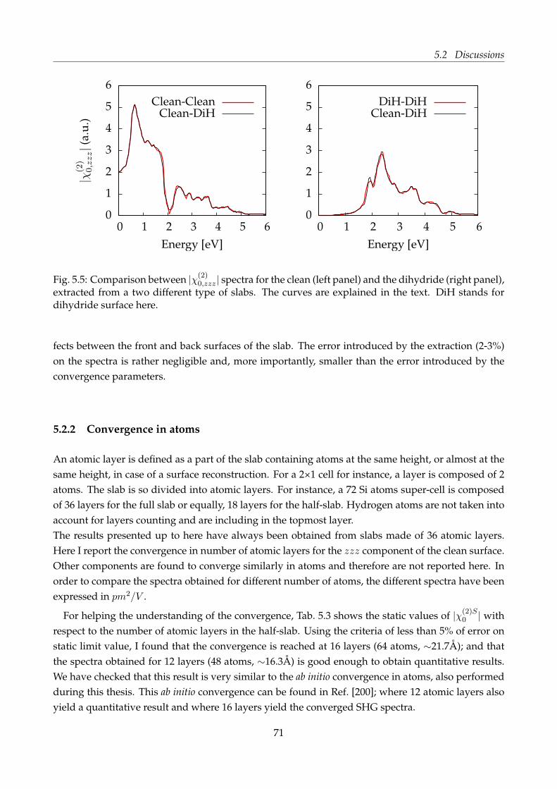
5.2 Discussions
Fig. 5.5: Comparison between |χ(2)0,zzz| spectra for the clean (left panel) and the dihydride (right panel),
extracted from a two different type of slabs. The curves are explained in the text. DiH stands fordihydride surface here.
fects between the front and back surfaces of the slab. The error introduced by the extraction (2-3%)on the spectra is rather negligible and, more importantly, smaller than the error introduced by theconvergence parameters.
5.2.2 Convergence in atoms
An atomic layer is defined as a part of the slab containing atoms at the same height, or almost at thesame height, in case of a surface reconstruction. For a 2×1 cell for instance, a layer is composed of 2atoms. The slab is so divided into atomic layers. For instance, a 72 Si atoms super-cell is composedof 36 layers for the full slab or equally, 18 layers for the half-slab. Hydrogen atoms are not taken intoaccount for layers counting and are including in the topmost layer.The results presented up to here have always been obtained from slabs made of 36 atomic layers.Here I report the convergence in number of atomic layers for the zzz component of the clean surface.Other components are found to converge similarly in atoms and therefore are not reported here. Inorder to compare the spectra obtained for different number of atoms, the different spectra have beenexpressed in pm2/V .
For helping the understanding of the convergence, Tab. 5.3 shows the static values of |χ(2)S0 | with
respect to the number of atomic layers in the half-slab. Using the criteria of less than 5% of error onstatic limit value, I found that the convergence is reached at 16 layers (64 atoms, ∼21.7Å); and thatthe spectra obtained for 12 layers (48 atoms, ∼16.3Å) is good enough to obtain quantitative results.We have checked that this result is very similar to the ab initio convergence in atoms, also performedduring this thesis. This ab initio convergence can be found in Ref. [200]; where 12 atomic layers alsoyield a quantitative result and where 16 layers yield the converged SHG spectra.
71

Chapter 5. Microscopic theory of surface second-harmonic generation
Fig. 5.6: Convergence of |χ(2)S0,zzz| in number of atomic layers. The
numbers of layers indicated correspond to the numbers of atomiclayers in half of the slab. To be converted in numbers of atoms,they have to be multiplied by 2 because the clean surface has twoatoms per layer, and by another factor of 2 for the two half of theslab.
N. layers Static value[×10−19 pm2/V]
8 7.1710 8.7012 9.3914 9.0716 9.8518 9.9124 9.9630 9.95
Tab. 5.3: Static value of |χ(2)S0,zzz|
for the clean surface.
5.2.3 Two-bands contribution
In the special case of α = β = γ and when the first momentum matrix element is not a modifiedmomentum matrix element, the two-bands contribution, given by Eq. (5.22b), reads as
χ2bndααα (ω) =
i
V
∑
nn′
BZ∑
k
fnm〈n,k|pα|n′,k〉〈n′,k|pα|n,k〉〈n′,k|∆α|n,k〉E4
n′n(k)
[
16
(En′n(k)− 2ω)− 1
(En′n(k)− ω)
]
.
From the time-reversal symmetry, one obtains that χ2bndααα (ω) = 0. This property can be used in SHG
codes to optimise the calculation of χ(2)0 for the components such as α = β = γ.
One could be interested by proving an equivalent result for the surface two-band contribution. In thesurface case, 〈n,k|pα|n′,k〉 is replaced by 〈n,k|Pα|n′,k〉. Thus, the two momentum matrix elementsare now a momentum matrix element and a modified momentum matrix element. There are no moreequivalent by the time-reversal symmetry. Therefore, if we want to compute the half-slab spectra, thetwo-bands contribution must always be computed.
5.2.4 Symmetric or asymmetric slab
In this section, we use the fact that the half-slab and the full-slab spectra in the linear spectra dif-fer only by a factor of 2. In Fig.5.7, a comparison between the linear full slab and extracted spectraof the clean Si(001) surface is reported. In the left panel, the total spectra divided by two (full slabcalculation from the clean-clean slab) is compared with the extracted spectra from the clean-cleanslab. In the right panel, the same total spectra divided by two is compared with the extracted spectra
72

5.2 Discussions
Fig. 5.7: Top panels: Comparison between linear spectra obtained from two different systems, asymmetric slab ( clean-clean ) and an asymmetric slab ( clean-dihydride ), using the tight-bindingcode. Total refers to full slab calculation from the clean-clean slab. Bottom panels: difference betweenfull slab over two and half slab calculations.
from a clean-dihydride slab. The quantity reported is Im(ǫxx − ǫyy), in order to overcome the bulkcontribution. The bulk being isotropic, this allows us to discuss only about the surface contribution.Notice that this quantity is close to the reflectance anisotropy spectroscopy (RAS).In the linear case, if the spectrum is computed from a symmetric slab, i.e., front and back surfacesbeing identical; we obtain exactly, by extraction, one half of the total spectra. This is verified in thelower left panel, showing the difference of the two spectra. This has already been pointed out, see,for instance Ref. [182]. On the contrary, if the spectrum is extracted from an asymmetric slab, there isa small but visible discrepancy between the two spectra.Even if it is not possible to access as easily to the SHG surface spectra, we expect that using a symmet-ric slab leads to better results in SHG too. In Chap. 7, it is proven analytically that the slab must bechosen symmetric if one wants to be able to compute the macroscopic second-harmonic generation.
5.2.5 Tight-binding picture of Cz1
Let us consider a basis of orbitals, localized on atoms. This basis-set of orbitals is assumed to beorthogonal. Any Bloch state can be expressed in this basis as
|n,k〉 =∑
i
∑
αi
cnαi(k)|α, i〉,
where i refers to the atoms and αi is the orbitalsα attached to the atom i, and cnαi(k) are the coefficients
of the Bloch state |n,k〉, in the orbital basis.
73

Chapter 5. Microscopic theory of surface second-harmonic generation
In this basis, a matrix element of the momentum can be written as [201, 202]
〈n,k|p|n′,k〉 =∑
i,j
∑
αi,βj
cn†αi(k)cn
′βj(k)∇αi,βj
. (5.24)
Starting from (5.3), it is possible to rewrite that formula as
χ(2)S0,abc(ω) = − 1
2V ω3
∑
n,n′,n′′,k
Im(PPart,an,n′ (k)(pbn′,n′′(k)pcn′′,n(k) + pcn′,n′′(k)pbn′′,n(k)))
En,k − En′,k + 2ω + 2iη[
fnn′′
En,k − En′′,k + ω + iη+
fn′n′′
En′′,k − En′,k + ω + iη
]
, (5.25)
with
PPartn,n′ (k) = 〈nk|C(z)p|n′k〉 =
∑
i,j
C(zi)∑
αi,βj
cn†αi(k)cn
′βj(k)∇αi,βj
,
where C(zi) is 1 if the atom i, located at the height zi, is inside the half-slab defined by C(z). Here wedefined ∇αi,βj
= 〈α, i|∇H0|β, j〉. For obtaining this expression, we explicitly used the tight-bindingexpression of the matrix elements given by Eq. (5.24); and therefore Eq. (5.25) is only valid in thetight-binding limit.We can now write more explicitly PPart,a
n,n′ (k)(vbn′,n′′(k)vcn′′,n(k)+vcn′,n′′(k)vbn′′,n(k)) in the tight-binding
formalism.So putting all together, we get
PPart,an,n′ (vbn′,n′′vcn′′,n + vcn′,n′′vbn′′,n) =
∑
i
C(zi)∑
j
∑
αiβj
cn†αicn
′βj∇a
αiβj(vbn′,n′′vcn′′,n + vcn′,n′′vbn′′,n). (5.26)
Inserting Eq. (5.26) into Eq. (5.25), we obtain a formula where it appears explicitly a sum over theatoms in front of the expression, weighted by the cut-function C(z) evaluated at the height zi of theatoms. Therefore χ(2)S
0 is constructed by adding the individual contributions of each atom. Eachatom playing an independent role, we can decide how to construct a spectra. For instance, the half-slab spectra can be computed choosing C(z) as the indicator function of the half-slab. Or it canbe constructed by adding the individual contributions of the atomic layers forming the half-slab,computed separately. Mathematically, this function C(z) describes a partition over the atoms. A directconsequence is the possibility to perform a layer-by-layer analysis of the surface second-harmonicgeneration spectra. Therefore in next section, I exploit this result to analyse the spatial constructionof the second-harmonic spectra.
5.2.6 Spatial construction of the SHG spectra
As mentioned above, the extraction procedure results to be a partition over the atoms, and each layercan be computed and analysed separately. The main motivation of this section is the understandingof the spatial construction of the SHG spectra.
74
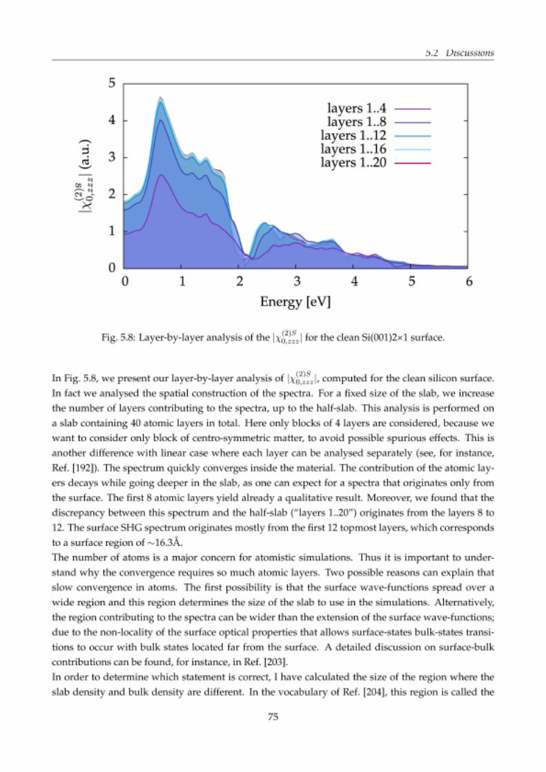

Chapter 5. Microscopic theory of surface second-harmonic generation
Fig. 5.9: Top panel: Variation of the number of electrons par Bohr along the z direction. This value isobtained by averaging the electronic density in the x−y plan for the entire cell. Bottom panel: relativedifferences between the bulk and the slab densities of the above panel. Note the change in the scale.The slab is composed of 16 atomic layers in total, with asymmetric dimers as surface reconstructionon both sides.
density surface region; by opposition to the optical surface region, where the optical properties of thesurface are different from bulk optical properties.Using the density obtained from an ab initio DFT calculation, it is possible to determine the depthof the density surface region. In order to present quantitative results, the density has been averagedin the plane perpendicular to the surface normal. The resulting quantity is shown in Fig. 5.9. Thedensity of the upper-most layers differs slightly from the value in the deeper layers and quickly re-covers the bulk density in the deeper layers. Using as a criteria that the slab and the bulk density areidentical if the relative difference is smaller than 0.5% (black dashed line, lower panel), I found thatthe density surface region is about 8.5 Å.8
By comparing this value to the optical surface region size (estimated above to be ∼16.3Å), we directlyobtain that the optical surface region is wider than the density surface region; as already found inRef. [205] for the semi-classical infinite barrier model. Physically, this originates from the fact that theoptical properties of surfaces are non-local and by consequence, the optical response lives on a widerregion than the density surface region. This allows the aforementioned bulk-states surface-states
8This value of 0.5% is here fixed by the numerical noise on the signal and under this value, the two signals can beconsidered as equal.
76
5.2 Discussions
transitions to occur deeper inside the material than the density surface region. Even if the changesof the density induced by the presence of the surface (and therefore the surface wave-functions) arewell described, the correct description of the optical properties of surfaces requires more layers to beconverged.
Conclusions
In this chapter, I have investigated the theory behind the calculation of the surface second-harmonicgeneration within the super-cell approach. More precisely, we have seen how it is possible to extractthe spectrum containing only the contribution of a single surface, within the independent-particleapproximation.We have first analysed the different choices offered by the literature in order to access the SHG spec-tra in super-cell geometry. Invoking the gauge invariance, we have reduced to one the number ofpossible formulae for extracting the spectra. This formula have then been derived by integrating themicroscopic current over half of the slab. In the case of clean Si(001) surface, we found that when itis possible to access to the exact spectra, our method reproduce surprisingly well the correct spectra,thus validating our approach. Interestingly, we have recovered the formula adopted by the majorityof the literature, validating their choice.I have also discussed about numerical accuracy of the extraction procedure, showing that a smallerror of 2-3% is expected. It has been verified by tight-binding calculations on silicon surfaces thatthe two surfaces of a finite slab are independent. Using the fact that our approach turns to be apartition over the atoms in the tight-binding limit, we have analysed the spatial construction of thespectra, performing a layer-by-layer analysis. The calculations show that surface spectra originatesfrom the top-most atomic layers and that the contribution decays when going far from the surface.More precisely, I found that the spectra mainly originates from the 12 topmost layers. Going furtherI explained that the number of atomic layers required for a converged calculation is governed bythe non-locality of the response function χ(2)S
0 and not by the spatial extension of the surface wave-functions.
To conclude, the calculation of the surface second-harmonic generation is now based on a solidtheoretical ground. Nevertheless, only the microscopic response can be described by the theory pre-sented in this chapter. In the next chapter, the microscopic theory is improved by the inclusion of theeffects of nonlocal operators. The macroscopic theory of surface second-harmonic generation is thenpresented in Chapter 7.
77


6. Effects of nonlocal operators on surfacesecond-harmonic generation
The most used framework for ab initio calculations, density-functional theory within the local-densityapproximation [97], underestimates the energy band gap of semiconductors. It is now well under-stood that solving the DFT equations using a Kohn-Sham scheme should not yield the correct band-gap [88]. In this context, the so-called GW approximation [112] is known to correct the electronic gapof most semiconductors [206]. However, this can be a very expensive calculation and thus one usesthe much simpler scissors operator scheme [207–209], which is still a nonlocal operator. This allowsus to “open” the DFT gap to its correct experimental or GW value for most bulk semiconductors.This approximation has already been used in the calculation of the linear optical properties of sur-faces [210, 211], thus improving the agreement with the experimental results.DFT calculations are often based on the use of pseudopotentials; and as mentioned previously, thisis the case for all the ab initio calculations of this thesis. As it will be discussed in this chapter, thepresence of a nonlocal part of the pseudopotential introduces corrections to the momentum operatorof the electron that have to be included with care in the surface second-harmonic susceptibility [212].For the bulk counterpart, see, for instance, Ref. [213]. For linear optical properties of surfaces includ-ing the cut-function C(z), see, for instance, Ref. [121].Therefore, within the independent-particle approximation, the most complete approach for the calcu-lation of the surface second-harmonic susceptibility is one which includes (i) the scissors correction,(ii) the contribution of the nonlocal part of the pseudopotential, and (iii) the cut function C(z) intro-duced in the previous chapter. Therefore the goal of this chapter is to derive a new expression withinthe length-gauge for the surface second-harmonic susceptibility tensor that includes the aforemen-tioned contributions. The inclusion of these three contributions opens the possibility to study surfaceSHG with more versatility and to provide accurate results.Partial account of this work has already been published in Ref. [200]. Here, I give a detailed descrip-tion of the theory and the method of calculation; in particular I present the evaluation of the densitysurface response function using perturbation theory, starting from the second-order induced current.By opposition to Ref. [200], here I do not use the density-matrix formalism. This gives an other wayfor obtaining the surface second-order susceptibility, but more interestingly, it opens the way to gobeyond the IPA. As explained in Chap. 3, the density-density-density response function computedwithin the independent-particle approximation enters as the key ingredient for computing the fully-interacting density-density-density response function.
79
Chapter 6. Effects of nonlocal operators on surface second-harmonic generation
In this chapter, I first present the relevant steps for deriving the surface second-order susceptibilitytensor χ(2)
0 . This derivation includes the addition of the terms mentioned above that have been ab-sent in previous works. Then I compare results from before and after adding the different nonlocalcontributions.
6.1 Nonlocal operators and perturbation theory
6.1.1 Nonlocal operators in TDDFT
We assume the IPA, a classical electromagnetic field, quantum-mechanical matter and we neglectlocal-field and excitonic effects.The unperturbed Hamiltonian, describing the system in absence of any interaction, includes in somecases nonlocal operators. As explained in the introduction of this chapter, I focus on two nonlocaloperators, one originating from the pseudo-potential approximation and the second one accountingfor the screening of particles inside the materials.This unperturbed Hamiltonian is used to solve the Kohn-Sham equations (see Chap. 3). As in thisthesis I work within the local-density approximation, the Hamiltonian is labelled with the corre-sponding LDA superscript. Any other approximation can be used (like the generalized-gradientapproximation) and the derivation remains the same.Then,
HLDA0 (r, p) =
p2
2+ Veff(r), (6.1)
with p = −i∇ its canonical momentum, and Veff the effective potential, where we neglect spin-orbitterms.To be general in our derivation of χ(2)
0 , we assume a nonlocal contribution as it is customary for mostpseudopotentials, and then we replace the local effective potential Veff(r) with
Veff(r, p) = V l(r) + V nl(r, p), (6.2)
where V l(r) and V nl(r, p) are the local and nonlocal parts, respectively. The argument (r, p) is equiv-alent to the explicit (r, r′) nonlocal notation [212]. In case of a local potential, i.e., Veff = V l(r), likethat of all-electron schemes, we simply omit the contribution of V nl(r, p) from the results that wehave derived.It is well known that the use of the LDA leads to an underestimation of the band-gap. A standardprocedure to correct for this is to use the “scissors approximation”, where the conduction bands arerigidly shifted in energy so that the band-gap corresponds to the accepted experimental electronicband-gap [207–209]. This is often in fairly good agreement with the GW band-gap based on a moresophisticated calculation [214]. The LDA wave-functions are used since they produce band structureswith dispersion relations similar to those predicted by the GW approximation. One might wonder ifthis approximation is still valid for the surface states. Taking the clean Si(001) surface as an example,one clearly see in Fig. 6.1 that the GW surface states exhibit the same dispersion as the LDA ones.Mathematically, the scissors operator S is a nonlocal operator which is added to the unperturbed or
80

6.1 Nonlocal operators and perturbation theory
Fig. 6.1: Calculated surface states of Si(001)2×1 using LDA (dashed lines) and GW (solid lines). Sym-bols corresponds to photoemission experiments [215]. Reproduced from [215].
unscissored Hamiltonian HLDA0 ,
HΣ0 (r, p) = HLDA
0 (r, p) + S(r, p), (6.3)
where
S(r, p) = ∆∑
n
BZ∑
k
(1− fn,k)|n,k〉〈n,k|, (6.4)
with ∆ the rigid (k-independent) energy correction to be applied. The unscissored and scissoredHamiltonians satisfy
HLDA0 (r, p)φn,k(r) = En(k)φn,k(r),
HΣ0 (r, p)φn,k(r) = EΣ
n (k)φn,k(r),
where the scissor-shifted energies EΣn (k) are given by
EΣn (k) = En(k) + (1− fn,k)∆.
We emphasize that the scissored and unscissored Hamiltonians have the same eigenfunctions, whereφn,k(r) = 〈r|n,k〉 = eik.run,k(r), are the real-space representations of the Bloch states |n,k〉 labelledby the band index n and the crystal momentum k, and un,k(r) are cell-periodic.
6.1.2 Coupling nonlocal operators to the electromagnetic field
In presence of a nonlocal operator, the treatment of the coupling to the electromagnetic field requiresgreat care.
81

Chapter 6. Effects of nonlocal operators on surface second-harmonic generation
Let us consider the total single-electron Hamiltonian H(t) that reads as
H(t) = H0 + HI(t),
where H0 is the unperturbed one-particle time-independent Hamiltonian (see Eq. 6.3), and HI(t)
is the time-dependent potential energy due to the interaction of the electron with the perturbingelectromagnetic field.The interaction Hamiltonian in the presence of a nonlocal potential V nl is given by [212]
HI(t) = φP (t)− 1
2c
[
pAP (t) + AP (t)p]
+1
2c2AP (t)2 + V A
nl (t), (6.5)
where φP is the scalar potential, AP the vector potential, and
〈r|V Anl |r′〉 = V nl(r, r′)
∞∑
k=1
1
k!
(
i
c
∫ r
r′AP (x, t). dx
)k
. (6.6)
Here, we are interested in a perturbative treatment of the interaction, therefore, the interaction Hamil-tonian is expanded in power of AP (r, t).First- and second-order terms, which are required to treat the linear and the second-order nonlinearoptical properties, are given by
H(1)I (r, r′, t) = φP (r, t)− 1
2c
[
pAP (r, t) +AP (r, t)p]
+ Vnl(r, r′)i
c
∫ r
r′AP (x, t). dx,
H(2)I (r, r′, t) =
1
2c2AP (r, t)2 − Vnl(r, r
′)1
c2
(
∫ r
r′AP (x, t). dx
)2
.
To overcome integrals, I assume the long-wavelength limit; which corresponds to the replacementAP (r, t) → AP (t). Using the fact that V nl(r, r′)(r − r′) = [r, V nl] and using the definition of thevelocity operator v = p− i[r, V nl], we obtain after simple algebra that
H(1)I (t) = φP (t)− 1
cvAP (t),
H(2)I (t) =
−i2c2
[AP (t)r,AP (t)v].
(6.7)
These two expressions are very close to the usual one, obtained in absence of nonlocal operators.Here as a result, one obtains that in presence of nonlocal operators, the momentum operator p mustbe replaced by the velocity operator v in the expression of the first- and second-order terms of theinteraction Hamiltonian.Knowing the first- and second-order interaction Hamiltonians, it is possible to derive from perturba-tion theory, the expression of the second-order susceptibility. This is the aim of the next section.
82
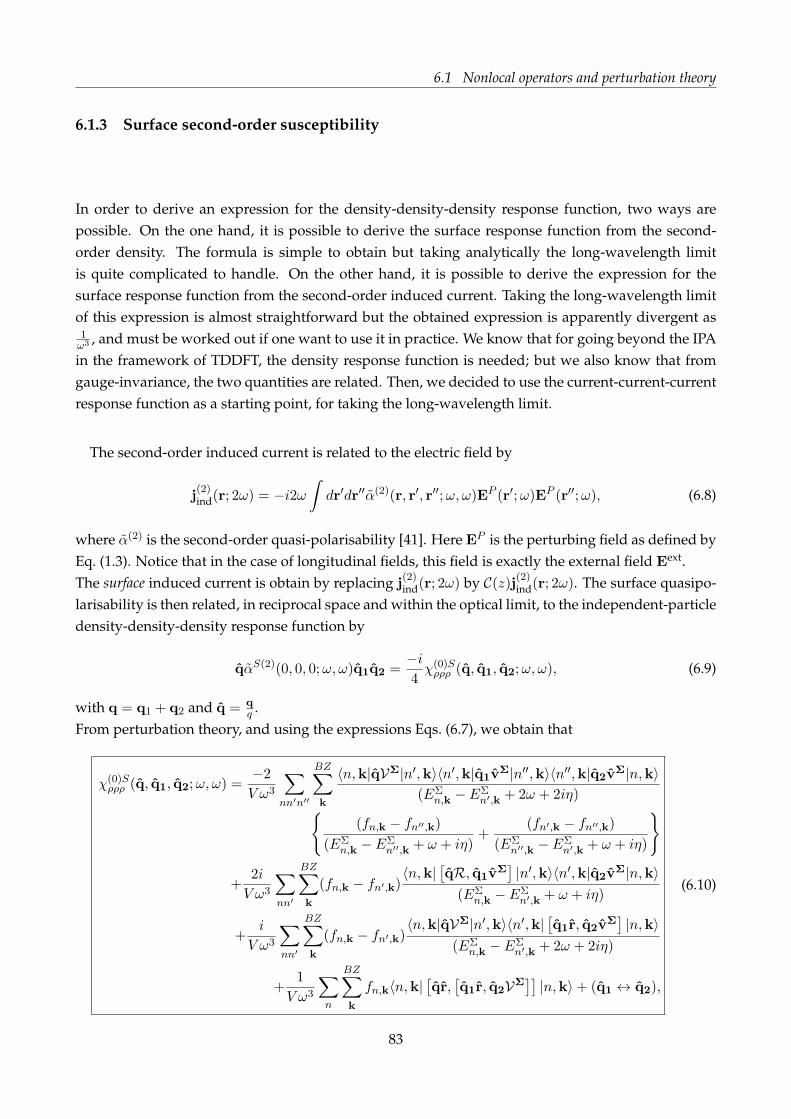
6.1 Nonlocal operators and perturbation theory
6.1.3 Surface second-order susceptibility
In order to derive an expression for the density-density-density response function, two ways arepossible. On the one hand, it is possible to derive the surface response function from the second-order density. The formula is simple to obtain but taking analytically the long-wavelength limitis quite complicated to handle. On the other hand, it is possible to derive the expression for thesurface response function from the second-order induced current. Taking the long-wavelength limitof this expression is almost straightforward but the obtained expression is apparently divergent as1ω3 , and must be worked out if one want to use it in practice. We know that for going beyond the IPAin the framework of TDDFT, the density response function is needed; but we also know that fromgauge-invariance, the two quantities are related. Then, we decided to use the current-current-currentresponse function as a starting point, for taking the long-wavelength limit.
The second-order induced current is related to the electric field by
j(2)ind(r; 2ω) = −i2ω
∫
dr′dr′′α(2)(r, r′, r′′;ω, ω)EP (r′;ω)EP (r′′;ω), (6.8)
where α(2) is the second-order quasi-polarisability [41]. Here EP is the perturbing field as defined byEq. (1.3). Notice that in the case of longitudinal fields, this field is exactly the external field Eext.The surface induced current is obtain by replacing j
(2)ind(r; 2ω) by C(z)j(2)ind(r; 2ω). The surface quasipo-
larisability is then related, in reciprocal space and within the optical limit, to the independent-particledensity-density-density response function by
qαS(2)(0, 0, 0;ω, ω)q1q2 =−i4χ(0)Sρρρ (q, q1, q2;ω, ω), (6.9)
with q = q1 + q2 and q = qq .
From perturbation theory, and using the expressions Eqs. (6.7), we obtain that
χ(0)Sρρρ (q, q1, q2;ω, ω) =
−2
V ω3
∑
nn′n′′
BZ∑
k
〈n,k|qVΣ|n′,k〉〈n′,k|q1vΣ|n′′,k〉〈n′′,k|q2v
Σ|n,k〉(EΣ
n,k − EΣn′,k + 2ω + 2iη)
(fn,k − fn′′,k)
(EΣn,k − EΣ
n′′,k + ω + iη)+
(fn′,k − fn′′,k)
(EΣn′′,k − EΣ
n′,k + ω + iη)
+2i
V ω3
∑
nn′
BZ∑
k
(fn,k − fn′,k)〈n,k|
[
qR, q1vΣ]
|n′,k〉〈n′,k|q2vΣ|n,k〉
(EΣn,k − EΣ
n′,k + ω + iη)
+i
V ω3
∑
nn′
BZ∑
k
(fn,k − fn′,k)〈n,k|qVΣ|n′,k〉〈n′,k|
[
q1r, q2vΣ]
|n,k〉(EΣ
n,k − EΣn′,k + 2ω + 2iη)
+1
V ω3
∑
n
BZ∑
k
fn,k〈n,k|[
qr,[
q1r, q2VΣ]]
|n,k〉+ (q1 ↔ q2),
(6.10)
83

Chapter 6. Effects of nonlocal operators on surface second-harmonic generation
where we have introduced the following definitions
VΣ =
vΣC(z) + C(z)vΣ
2,
R = C(z)r.(6.11)
In presence of the nonlocal part of the pseudopotential and a scissors operator, the velocity vΣ isgiven by
vΣ = p+ vnl + vS = v + vS,
vnl = −i[r, V nl],
vS = −i[r, S].(6.12)
It is important to note first that in absence of any nonlocal operator, the Eq. (6.10) reduces to its firstterm only; which is the expression previously obtained (see Eq. 5.3). By opposition to the expressionsof the interaction Hamiltonian, where the nonlocal operators accounts only for the replacement p →vΣ, in the case of the surface susceptibilities, extra-terms must be including.Even if Eq. (6.10) allows us in principle to compute the surface density-density-density responsefunction, this expression is not satisfactory for two reasons. i) The expression Eq. (6.10) is apparentlydivergent as 1
ω3 ; which prohibits numerical implementations. ii) This expression contains matrixelements of vΣ. This last remark comes from the fact that the matrix elements of v and vΣ (asdefined by Eq. (6.12)) are related each others
rnn′(k) =vΣnn′
iEΣnn′(k)
=vnn′
iEnn′(k), n /∈ Dn′ ,
where we defined EΣnm(k) = EΣ
n (k)− EΣm(k) and Dm are all the possible degenerate m-states.
After tedious algebra, reported in App. E, one finally obtains a non-divergent expression of the sur-face second-order susceptibility, where the matrix elements of vΣ have been analytically replaced bymatrix elements of v. The final expression reads as
χ(0)Sρρρ = χ3bnd
I + χ3bndII + χ2bnd
l + χ2bndnl , (6.13)
where
χ3bndI (q, q1, q2, ω, ω) =
2i
V
∑
n 6=n′ 6=n′′
BZ∑
k
〈n,k|qR|n′,k〉〈n′,k|q1r|n′′,k〉〈n′′,k|q2r|n,k〉
×
(En,k + En′,k − 2En′′,k)
Enn′(k)
4(fn,k − fn′,k)
EΣnn′(k)(EΣ
nn′(k) + 2ω + iη)
+(2En,k − En′,k − En′′,k)
En′′n(k)
(fn,k − fn′′,k)
EΣnn′′(k)(EΣ
nn′′(k) + ω + iη)
+(2En′,k − En,k − En′′,k)
En′n′′(k)
(fn′,k − fn′′,k)
EΣn′n′′(k)(EΣ
n′′n′(k) + ω + iη)
+ (q1 ↔ q2) (6.14a)
84

6.1 Nonlocal operators and perturbation theory
χ3bndII (q, q1, q2;ω, ω) =
4i
V
∑
n 6=n′ 6=n′′
BZ∑
k
〈n,k|qR|n′,k〉〈n′,k|q1r|n′′,k〉〈n′′,k|q2r|n,k〉(2EΣ
n′′n(k)− EΣn′n(k))
×
2(fn,k − fn′,k)
(EΣnn′(k) + 2ω + 2iη)
− (fn,k − fn′′,k)
(EΣnn′′(k) + ω + iη)
+(fn′,k − fn′′,k)
(EΣn′′n′(k) + ω + iη)
+ (q1 ↔ q2) (6.14b)
χ2bndl (q, q1, q2;ω, ω) =
−2
V
∑
n 6=n′
BZ∑
k
(fn,k − fn′,k)〈n,k|qR|n′,k〉〈n′,k|q1r|n,k〉q2∆n′n
EΣnn′(k)2
×
8(Enn′(k) + EΣnn′(k))
EΣnn′(k)(EΣ
nn′(k) + 2ω + 2iη)+
(2Enn′(k)− EΣnn′(k))
EΣnn′(k)(EΣ
nn′(k) + ω + iη)
+ (q1 ↔ q2) (6.14c)
χ2bndnl (q, q1, q2;ω, ω) =
−2
V
∑
nn′
BZ∑
k
(fn,k − fn′,k)
Enn′(k)EΣnn′(k)
〈n,k|[qR, q1v]|n′,k〉〈n′,k|q2r|n,k〉(EΣ
nn′(k) + ω + iη)
+4〈n,k|qR|n′,k〉〈n,k|[q1r, q2v]|n′,k〉
(EΣnn′(k) + 2ω + iη)
+ (q1 ↔ q2) (6.14d)
where we defined ∆n′n = vn′n′ − vnn and
〈n,k|R|n′,k〉 = 〈n,k|V |n′,k〉iEnn′(k)
, n /∈ Dm.
It is interesting to note that each specific contribution incorporated in that expressions (the scissorsoperator, the nonlocal part of the pseudo-potential, and the cut-function C(z)) play separate andindependent roles. The cut-function C(z) here only affects the matrix element related to q. Thescissors operator only affects the energies and finally, the nonlocal part of the pseudo-potential isaccounted for by computing matrix elements of v, instead of p.As already pointed out in Ref. [41] for the bulk susceptibility, the scissored and unscissored energiesare both present in the expression of χ(0)S
ρρρ , showing that the scissors operator is non-trivial for second-order susceptibility.By opposition, the expression for the surface first-order density response function χ(0)S
ρρ is given by
χ(0)Sρρ (q;ω) =
1
V
∑
nn′
BZ∑
k
(fn,k − fn′,k)〈n,k|qR|n′,k〉〈n′,k|qr|n,k〉
(EΣn,k − EΣ
n′,k + ω + iη), (6.15)
where only scissored energies appear, resulting in a rigid shift of the spectra by ∆.The expression of the second-order susceptibility is now satisfactory for various reasons. First, be-cause this form is non-divergent. Second, for practical implementations, the scissors and the nonlocalpart of the pseudo-potential can be easily switch on and off by replacing EΣ
n (k) by En(k) in the firstcase and v by p in the second. Finally, the bulk formula is obtained by replacing R by r. Thus, byimplementing only one formula, it is possible to treat easily all the possible different combinationsof the three contributions. This is that expression which has been implemented in the TDDFT code2light [117]. The analytical expression of V is given in App. D.
85

Chapter 6. Effects of nonlocal operators on surface second-harmonic generation
6.2 Numerical results
The self-consistent ground-state and the Kohn-Sham states were calculated using the plane-waveABINIT code [115]. We used Troullier-Martins pseudopotentials [216] that are fully separable nonlo-cal pseudopotentials in the Kleinman-Bylander form [120]. The contribution of the nonlocal part ofthe pseudo-potential to v and V is carried out using the DP code [116].The vacuum size is equivalent to one quarter the size of the slab, avoiding the effects producedby possible interaction between the replicas of the slab always present in the repeated super-cellscheme [217].Spin-orbit, local-field, and electron-hole attraction effects on the SHG process are all neglected atthis point. Although these are important factors in the optical response of a semiconductor, theirefficient calculation is theoretically and numerically challenging. They will be treated later in thisthesis. In order to obtain χ2bnd
nl , we must evaluate the commutator of r and vnl. Computing second-order derivatives of the nonlocal part of the pseudo-potential is required thus making the numericalprocedure very time consuming. This adds significantly to the already lengthy time needed for thecalculation of the vnl contribution that is proportional only to the first order derivatives. Memoryrequirements are also increased for both vnl and [r, vnl]. However, the contribution from [r, vnl] isvery small [218] and therefore we neglect entirely χ2bnd
nl from now on.1
For a given slab of 32 atomic layers, we find the converged spectra to obtain the relevant parame-ters. The most important of these are: an energy cutoff of 10 Ha, an equal number of conduction andvalence bands, and a set of 244 k-points. The k-points are used for the linear analytic tetrahedronmethod for evaluating the 3D Brillouin-zone (BZ) integrals where special care was taken to exam-ine the double resonances of Eq. (6.14) [219]. Note that the Brillouin zone for the slab geometrycollapses to a 2D zone, with only one k-point along the z axis. All spectra were calculated with aGaussian smearing of 0.15 eV. The reader should note that numerical results presented here are thesame results as published in Ref. [200].
6.2.1 Half-slab vs. full slab
In Fig. 6.2, we compare χfullslab0,xxx versus χhalf−slab
0,xxx for the four different possibilities between includingor not including the effects of vnl or the scissors correction ∆. For these results, we chose ∆= 0.5 eV,that is, the GW gap reported in Refs. [215, 220]. This is justified by the fact that the surface statesof the clean Si(001) surface are rigidly shifted and maintain their dispersion relation with respect toLDA according to the GW calculations of Ref. [220]. We see that for all four instances the differencebetween responses is quite small. Indeed, when the value |χ(2)
0,xxx| is large, the difference between thetwo is very small; when the value is small the difference increases only slightly, but the spectra is soclose to zero that it is negligible. These differences would decrease as the number of atomic layersincreases. As already explained in the previous chapter, we remark here that 32 layers in the slab ismore than enough to confirm that the extraction of the surface second-harmonic susceptibility fromthe 2×1 surface is readily possible using the formalism contained in Eq. (6.13).
1This approximation is valid for [r, vnl] but could not be applied to [r, vS]. This is why it is important to first replaceanalytically vΣ by v.
86
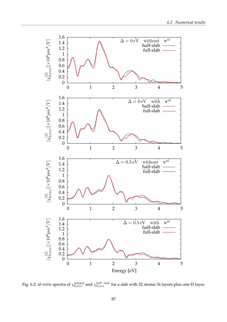
6.2 Numerical results
Fig. 6.2: ab initio spectra of χfullslab0,xxx and χhalf−slab
0,xxx for a slab with 32 atomic Si layers plus one H layer.
87

Chapter 6. Effects of nonlocal operators on surface second-harmonic generation
Fig. 6.3: |χ2×10,xxx| versus the photon energy for a slab with 32 atomic Si layers plus one H layer, with
and without the contribution from vnl. Spectra are obtained with ∆= 0.5 eV.
6.2.2 Results for χ2×10,xxx
We proceed to explain some of the features seen in |χ2×10,xxx| that are obtained by calculating |χhalf−slab
0,xxx |.First, from Fig. 6.2, we note a series of resonances that derive from 1ω and 2ω terms in Eq. (6.14).Notice that the 2ω resonances start below Eg/2 where Eg is the band gap (0.53 eV for LDA and1.03 eV if the scissor is used with ∆= 0.5 eV). These resonances come from the electronic states ofthe 2×1 surface, that lie inside the bulk band gap of Si and are the well known electronic surfacestates [220]. In Fig. 6.3, we see that the effect of vnl reduces the value of |χ2×1
0,xxx| by 15%-20% showingthe importance of this contribution for a correct calculation of surface SHG, in agreement with asimilar analysis for bulk semiconductors [213]. However, the inclusion of vnl does not change thespectral shape of |χ2×1
0,xxx|; this also can be confirmed from the cases of zero scissors correction fromFig. 6.2. To see the effect of the scissors correction, we take two different finite values for ∆. Thefirst one with a value of ∆= 0.5 eV, used in the above results, is the “average” GW gap taken fromRef. [220] that is in agreement with Ref. [215]. The second one with a value of ∆ = 0.63 eV is the“average” gap taken from Ref. [221], where more k-points in the Brillouin zone were used to calculateits GW value. From Fig. 6.4, we note that the scissors correction shifts the spectra from its LDAvalue to higher energies as expected. However, contrary to the case of linear optics [222] the shiftintroduced by the scissors correction is not rigid, as pointed out in Ref. [219]. This is because thesecond-harmonic optical response mixes 1ω and 2ω transitions (see Eq. (6.14)), and accounts for thenon-rigid shift. The reduction of the spectral strength is in agreement with the previous calculationsfor bulk systems [41, 219, 223].When we compare |χ2×1
0,xxx| for the two finite values of ∆, we see that the first two peaks are almostrigidly shifted with a small difference in height while the rest of the peaks are modified substantially.This behaviour comes from the fact that the first two peaks are almost exclusively related to the2ω resonances of Eq. (6.14). The other peaks are a combination of 1ω and 2ω resonances and yielda more modified spectrum. We mention that for large band-gap materials, the 1ω and 2ω wouldbe split showing a small interference effect, but still the 2ω would strongly depend on the surface
88
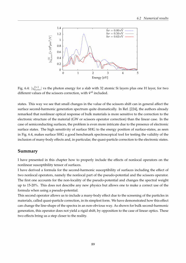
6.2 Numerical results
Fig. 6.4: |χ2×10,xxx| vs the photon energy for a slab with 32 atomic Si layers plus one H layer, for two
different values of the scissors correction, with vnl included.
states. This way we see that small changes in the value of the scissors shift can in general affect thesurface second-harmonic generation spectrum quite dramatically. In Ref. [224], the authors alreadyremarked that nonlinear optical response of bulk materials is more sensitive to the correction to theelectronic structure of the material (GW or scissors operator correction) than the linear case. In thecase of semiconducting surfaces, the problem is even more intricate due to the presence of electronicsurface states. The high sensitivity of surface SHG to the energy position of surface-states, as seenin Fig. 6.4, makes surface SHG a good benchmark spectroscopical tool for testing the validity of theinclusion of many-body effects and, in particular, the quasi-particle correction to the electronic states.
Summary
I have presented in this chapter how to properly include the effects of nonlocal operators on thenonlinear susceptibility tensor of surfaces.I have derived a formula for the second-harmonic susceptibility of surfaces including the effect oftwo nonlocal operators, namely the nonlocal part of the pseudo-potential and the scissors operator.The first one accounts for the non-locality of the pseudo-potential and changes the spectral weightup to 15-20%. This does not describe any new physics but allows one to make a correct use of theformula when using a pseudo-potential.This second operator allows us to include a many-body effect due to the screening of the particles inmaterials, called quasi-particle correction, in its simplest form. We have demonstrated how this effectcan change the line-shape of the spectra in an non-obvious way. As shown for bulk second-harmonicgeneration, this operator does not yield a rigid shift, by opposition to the case of linear optics. Thesetwo effects bring us a step closer to the reality.
89


Part III
Local-field effects in surface opticalproperties
91

7. Ab initio macroscopic linear andsecond-order optical properties ofcrystal surfaces:From the slab to the single surface
DON’T PANIC.
Douglas Adams, The Hitchhiker’s Guide to the Galaxy
As we have seen, the efficient approach for computing optical properties of surfaces relies on thesuper-cell approach and a slab geometry. However, this approach suffers intrinsically from the factthat a slab is composed of two surfaces. The definition of a surface dielectric tensor (or second-ordersusceptibility) remains unclear and the difference between the optical response of a thin film (made oftwo surfaces) and the optical response of a semi-infinite system, with a single surface, has not reallybeing investigated so far, in particular when local-field effects are included. In the linear case, the twosurfaces of a slab interfere constructively, making the mapping between slab calculations and surfaceoptical properties possible. However, as explained in Chap. 5, the direct calculation of the second-order optical properties is not possible in slab geometry, due to the destructive interferences betweenthe two surfaces of the slab. Even at the simple level of independent-particle approximation, wehave to introduce a cut-function, denoted here C(z), for being able to compute the second-harmonicgeneration from surfaces (see Chap. 5 and Chap. 6).This chapter aims to give the theoretical background for computing the macroscopic optical proper-ties of a single surface, from calculations performed in slab geometry.I refer in that chapter to the optical properties of half of the slab equally as half-slab or surface opticalproperties. In SHG, only the surface region contributes to the signal, justifying the use of the termsurface optical properties for the optical properties computed from half of the slab.This chapter is organised as follows. I first present how we can obtain from the microscopic compo-nents of the polarization, the in-plane averaged dielectric tensor
↔ǫm (q||, z, z
′;ω), keeping explicitlythe spatial fluctuations along the z direction [40]. From that expression, I give an expression forthat surface macroscopic dielectric tensor in the optical limit. I thus show that the longitudinal-longitudinal part of the macroscopic dielectric tensor can be computed from Time-Dependent Den-
93

Chapter 7. Ab initio macroscopic linear and second-order optical properties of crystal surfaces:From the slab to the single surface
sity Functional Theory (TDDFT).The second part of this chapter is dedicated to the extension of that calculation to the macroscopicsurface second-order response and follows the same organisation. Some properties of those newsurface response functions are finally discussed in Sec. 7.5.
7.1 Macroscopic dielectric tensor of crystal surfaces
In this section, I present in detail the derivation of the macroscopic dielectric tensor of half of a peri-odic system. Let us consider a system of electrons, perturbed by an external field Eext. Following thepaper of R. Del Sole and E. Fiorino [38], we express the polarization as the response to a perturbingfield EP , defined as
EP = Eext +Eind,T = E−Eind,L,
where E is the total microscopic field, and Eind,T and Eind,L are respectively, the transverse and thelongitudinal components of the field induced by the external perturbation.
The polarization is related to the perturbing field via the quasi-polarisability↔α and reads in Fourier
space as [38]
PG(q;ω) =∑
G′
[↔α (q;ω)
]
GG′EPG′(q;ω), (7.1)
where the notation PG(q) stands for P(q+G) and[↔α (q)
]
GG′ for↔α (q+G,q+G′).
It is shown in Ref. [38], that the polarization can be expressed as a response to the total electric fieldusing the expression
PG(q;ω) =[↔α (q;ω)
]
G0
↔Ar (q;ω)E0(q;ω), (7.2)
where↔Ar (q;ω) =
↔1 +4π q
qqq
[↔α(q;ω)
]
00
1−4π[αLL(q;ω)]00.
This formula is the starting point of this section. It is general and perfectly valid for any periodicsystem.Let us consider a super-cell, containing N atomic layers of thickness Lz and the same amount ofvacuum. In order to average over a selected region of the slab, we express the polarization in amixed-space (details can be found in App. A), where the in-plane periodicity is treated in reciprocalspace and the out-of-plane direction is treated in real space.Let us consider a function f of one variable in space. In real space, f is a function of the positionvector r and reads f(r). In reciprocal space, f is a function of a reciprocal vector k, that we can split,for periodic systems as super-cells, into a vector q belonging to the BZ plus a reciprocal lattice vectorG, and reads f(q + G). In the mixed-space, the in-plane periodicity is treated in reciprocal spacewhereas the out-of-plane direction is treated in real space. Therefore a function f reads in this spacef(q|| + G||, z) or fG||(q||, z), where q|| is a vector in the 2D BZ, G|| is an in-plane reciprocal-latticevector and z is the coordinate in the out-of-plane direction.The definitions of the corresponding Fourier transforms can be found in the App. A.Using Def. A.16,
PG||(q||, z;ω) =1
2Lz
∑
qz ,Gz
ei(qz+Gz)zPG(q;ω). (7.3)
94


Chapter 7. Ab initio macroscopic linear and second-order optical properties of crystal surfaces:From the slab to the single surface
the expression, with a clear derivation from the macroscopic Maxwell equations. The second point,more subtle, concerns the normalisation. As Eq. (7.7) is an average, we normalise there by half ofthe super-cell height, when averaging over half of the super-cell, leading to a well defined surface
dielectric tensor.Putting everything together, we obtain an expression for the macroscopic surface dielectric tensor
↔ǫS
M (q;ω) =↔1 +
4π
Lz
∑
Gz
C(−Gz)[↔α (q;ω)
]
Gz0
↔Ar (q;ω) =
↔1 +4π
↔αS
(q,q;ω)↔Ar (q;ω), (7.8)
where↔αS
is defined by the last part of the equation. Using the definition of↔Ar, we get directly that
↔ǫS
M (q;ω) =↔1 +4π
↔αS
(q,q;ω) + (4π)2
↔αS
(q,q;ω)qqqq
[↔α (q;ω)
]
00
1− 4π[
αLL(q;ω)]
00
. (7.9)
This result is very similar to Del Sole and Fiorino expression for the dielectric tensor of bulk ma-terials (see Eq. (25) of Ref. [38]), except that we have here a surface quantity. In Ref. [38], authorsalso obtained an expression for the macroscopic dielectric tensor. Their expression is very similar toEq. (7.6). Nevertheless, they obtained an expression defined thanks to an integral operator, whichplays the same role as
↔Ar in Eq. (7.6) (see Eq.(45) of Ref. [38]).
We also remark that not all ingredients of that formula are modified by the presence of the surface.This expression is general, in the sense that it gives access to all the components of the dielectrictensor. However, as explained in Chap. 1, it is possible to calculate the entire dielectric tensor in theoptical limit only from longitudinal-longitudinal (LL) calculations. Therefore, in the following wefocus only on the LL part of the surface dielectric tensor in the optical limit, as it corresponds to thescope of this chapter.
7.2 Optical limit for the surface macroscopic dielectric function
For the following, we restrict our discussion to the optical limit, which corresponds to a perturbationwith a vanishing momentum. This is valid for the low-energy region of the spectra where we areprecisely interested in.The key quantity in the optical limit is the longitudinal-longitudinal part of the macroscopic dielectricfunction ǫS,LLM . Only this quantity can be evaluated in the framework of TDDFT, where the electronicdensity is the fundamental physical quantity.From Eq. (7.9), the LL part of the surface macroscopic dielectric tensor reads as
ǫS,LLM (q;ω) = 1 + limq→0
4παS,LL(q,q;ω)
1− 4π[
αLL(q;ω)]
00
, q =q
q. (7.10)
Here, the quasi-polarisability α is related to response functions by [44]
↔α (r, r′;ω) = − 1
ω2
(
χ(1)jj (r, r′;ω)−
↔1 〈ρ〉δ(r− r′)
)
,
96
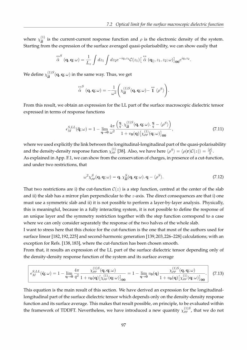
7.2 Optical limit for the surface macroscopic dielectric function
where χ(1)jj is the current-current response function and ρ is the electronic density of the system.
Starting from the expression of the surface averaged quasi-polarisability, we can show easily that
↔αS
(q,q;ω) =1
Lz
∫
dz1
∫
dz2e−iqzz1C(z1)
[↔α (q||, z1, z2;ω)
]
00eiqzz2 .
We define χ(1)Sjj (q,q;ω) in the same way. Thus, we get
↔αS
(q,q;ω) = − 1
ω2
(
χ(1)Sjj (q,q;ω)−
↔1 〈ρS〉
)
.
From this result, we obtain an expression for the LL part of the surface macroscopic dielectric tensorexpressed in terms of response functions
ǫS,LLM (q;ω) = 1− limq→0
4π
ω2
(
qq . χ
(1)Sjj (q,q;ω). qq − 〈ρS〉
)
1 + v0(q)[
χ(1)ρρ (q;ω)
]
00
, (7.11)
where we used explicitly the link between the longitudinal-longitudinal part of the quasi-polarisabilityand the density-density response function χ(1)
ρρ [38]. Also, we have here 〈ρS〉 = 〈ρ(r)C(z)〉 = 〈ρ〉2 .
As explained in App. F.1, we can show from the conservation of charges, in presence of a cut-function,and under two restrictions, that
ω2χSρρ(q,q;ω) = q. χS
jj(q,q;ω).q− 〈ρS〉. (7.12)
That two restrictions are i) the cut-function C(z) is a step function, centred at the center of the slaband ii) the slab has a mirror plan perpendicular to the z-axis. The direct consequences are that i) onemust use a symmetric slab and ii) it is not possible to perform a layer-by-layer analysis. Physically,this is meaningful, because in a fully interacting system, it is not possible to define the response ofan unique layer and the symmetry restriction together with the step function correspond to a casewhere we can only consider separately the response of the two halves of the whole slab.I want to stress here that this choice for the cut-function is the one that most of the authors used forsurface linear [182,192,225] and second-harmonic generation [139,203,226–228] calculations; with anexception for Refs. [138, 183], where the cut-function has been chosen smooth.From that, it results an expression of the LL part of the surface dielectric tensor depending only ofthe density-density response function of the system and its surface average
ǫS,LLM (q;ω) = 1− limq→0
4π
q2χ(1)Sρρ (q,q;ω)
1 + v0(q)[
χ(1)ρρ (q;ω)
]
00
= 1− limq→0
v0(q)χ(1)Sρρ (q,q;ω)
1 + v0(q)[
χ(1)ρρ (q;ω)
]
00
. (7.13)
This equation is the main result of this section. We have derived an expression for the longitudinal-longitudinal part of the surface dielectric tensor which depends only on the density-density responsefunction and its surface average. This makes that result possible, on principle, to be evaluated withinthe framework of TDDFT. Nevertheless, we have introduced a new quantity χ
(1)Sρρ , that we do not
97

Chapter 7. Ab initio macroscopic linear and second-order optical properties of crystal surfaces:From the slab to the single surface
know how to evaluate explicitly. This is the purpose of the next session.Notice that if we choose C(z) to be 1 everywhere, we recover the expression of the LL part of the di-electric function used for bulk materials [84], showing the consistency of our approach. We also notehere that χ(1)S
ρρ and χ(1)Sjj are not response functions; but they correspond to the surface macroscopic
average of response functions.
7.3 Calculation of ǫS,LLM in TDDFT
The last equation requires, for being evaluated, the expression of the two quantities χ(1)Sρρ (q,q;ω) and
χ(1)ρρ (q,q;ω), in the optical limit. The latter can be computed easily in TDDFT, but not the first one.
Eq. (7.13) can be rewritten as
ǫS,LLM (q;ω) = 1− limq→0
v0(q)1
Lz
∑
GzC(−Gz)
[
χ(1)ρρ (q;ω)
]
Gz0
1 + v0(q)[
χ(1)ρρ (q;ω)
]
00
. (7.14)
From now on, we assume the random-phase approximation.Under this approximation, the responsefunction of the fully interacting system χ
(1)ρρ is related to the independent-particle or Kohn-Sham
response function χ(0)ρρ of the (auxiliary) system by a Dyson-like equation, see Sec. 8.3.2,
[
χ(1)ρρ (q;ω)
]
GG′ =[
χ(0)ρρ (q;ω)
]
GG′ +∑
G1
[
χ(0)ρρ (q;ω)
]
GG1vG1
(q)[
χ(1)ρρ (q;ω)
]
G1G′ . (7.15)
Alternatively, one can introduce the response function to the total macroscopic classical potential χρρ
defined by [112, 229]
[
χρρ(q;ω)]
GG′ =[
χ(0)ρρ (q;ω)
]
GG′ +∑
G1
[
χ(0)ρρ (q;ω)
]
GG1vG1
(q)[
χρρ(q;ω)]
G1G′ , (7.16)
which implies that
[
χ(1)ρρ (q;ω)
]
GG′ =[
χρρ(q;ω)]
GG′ +[
χρρ(q;ω)]
G0v0(q)
[
χ(1)ρρ (q;ω)
]
0G′ , (7.17)
where vG(q) = vG(q) if G 6= 0 and 0 if G = 0.From Eq. (7.17), we obtain directly that χG0 = χG0
1+v0χ00, leading to
ǫS,LLM (q;ω) = 1− limq→0
v0(q)1
Lz
∑
Gz
C(−Gz)[
χρρ(q;ω)]
Gz0= 1− lim
q→0v0(q)χ
Sρρ(q,q;ω). (7.18)
For obtaining the quantity χS(q,q;ω), we have to solve the equation
χSρρ(q,q;ω) = χ(0)S
ρρ (q,q;ω) +∑
G1 6=0
χ(0)Sρρ (q,q+G1;ω)vG1
(q)[
χρρ(q;ω)]
G10, (7.19)
which is not a matrix equation, by opposition to Eq. (7.15) or Eq. (7.16). This makes the direct res-olution of this equation intricate. In order to solve that equation in a clever way, we introduce two
98

7.4 Macroscopic second-order tensor of crystal surfaces
matrices,[
χS(q;ω)]
GG′ and[
χ(0)Sρρ (q;ω)
]
GG′ .We define the matrix
[
χ(0)Sρρ (q;ω)
]
GG′ as
[
χ(0)Sρρ (q;ω)
]
0G′ = χ(0)Sρρ (q,q+G′;ω),
[
χ(0)Sρρ (q;ω)
]
GG′ =[
χ(0)ρρ (q;ω)
]
GG′ , G 6= 0.(7.20)
This corresponds to the replacement of the first line of the matrix[
χ(0)ρρ
]
GG′ by χ(0)Sρρ (q,q + G′;ω).
The matrix[
χSρρ(q;ω)
]
GG′ is defined similarly. From Eq. (7.19) and Eq. (7.16), and using the relationvG1
[
χρρ(q;ω)]
G10= vG1
[
χSρρ(q;ω)
]
G10, we obtain directly a matrix equation linking
[
χSρρ(q;ω)
]
GG′
to[
χ(0)Sρρ (q;ω)
]
GG′ ,
[
χSρρ(q;ω)
]
GG′ =[
χ(0)Sρρ (q;ω)
]
GG′ +∑
G1
[
χ(0)Sρρ (q;ω)
]
GG1vG1
[
χSρρ(q;ω)
]
G1G′ . (7.21)
Therefore, we have obtained a Dyson-like equation linking the matrix[
χSρρ
]
GG′ to the matrix[
χ(0)Sρρ
]
GG′ ;the latter being obtained from time-dependent perturbation theory. From Eq. (7.18),
[
χSρρ
]
00gives di-
rectly ǫS,LLM . Finally, we note that we can rework the expression of the surface macroscopic dielectricfunction for obtaining that
ǫS,LLM (q;ω) = limq→0
1(
1− v(q)χ(0)Sρρ (q,q;ω)
)−1
G=G′=0
. (7.22)
It is worthwhile to note that this expression is very similar to the expression for bulk crystals in theRPA, except that the independent-particle response function χ
(0)ρρ has been replaced by χ
(0)Sρρ . The
expression of the full matrix[
χ(0)Sρρ
]
GG′ is given in App. I, together with numerical results. Let usemphasize that this result allows us to describe how a surface affects the optical response of a ma-terial; with the convenience and efficiency of a super-cell calculation, assuming that the slab is thickenough do describe correctly the surface region. It was not obvious also that the surface dielectricfunction is obtained by solving the same equations than for bulk materials and in particular that theonly change at the end of the day is χ(0)
ρρ → χ(0)Sρρ . Also we note that χS
ρρ is an auxiliary matrix andonly the head of this matrix has a physical meaning.
7.4 Macroscopic second-order tensor of crystal surfaces
Let us consider now, instead of a linear polarization P = αEP , a polarization composed of twocontributions, a linear contribution P(1) associated to α(1) plus a second-order (in the perturbingfield) contribution P(2) associated to α(2). The aim of this section is to obtain an expression for themacroscopic surface second-order response function, following the approach used for the surfacedielectric tensor.
99

Chapter 7. Ab initio macroscopic linear and second-order optical properties of crystal surfaces:From the slab to the single surface
7.4.1 Microscopic components of the polarization
In order to be able to extend the linear calculation to the case of the second-harmonic generation, weneed all the microscopic components of the second-order polarization P
(2)G and not only the macro-
scopic one P(2)0 . Therefore, we do not follow here the derivation of Ref. [41].
In reciprocal space, the first- and second-order polarizations are given by [41]
P(1)G (q;ω) =
∑
G1
[↔α(1)
(q;ω)]
GG1EP
G1(q;ω), (7.23a)
P(2)G (q;ω) =
BZ∑
q1,q2
∑
G1,G2
∫
dω1dω2δ(ω − ω1 − ω2)δq,(q1+q2)
×[↔α(2)
(q,q1,q2;ω1, ω2)]
GG1G2EP
G1(q2;ω1)E
PG2
(q2;ω2), (7.23b)
where↔α(1)
and↔α(2)
are respectively the first- and second-order quasi-polarisabilities [41, 44]. In thefollowing, we always have ω = ω1 + ω2 and q = q1 + q2.From Maxwell equations, we obtain that
EPG(q;ω) = EG(q;ω) + 4π
q+G
|q+G|q+G
|q+G| .PG(q;ω). (7.24)
We note that this relation contains the first-order in polarization P(1) but also the second-order po-larization P(2).The perturbing field is the macroscopic applied perturbation and is of long wavelength, leading toEP
G(q;ω) = δG0EP0 (q;ω).
Inserting Eq. (7.24) into the expression of P(1)G , we obtain that
P(1)G (q;ω) =
[↔α(1)
(q;ω)]
G0E0(q;ω) + 4π
[↔α(1)
(q;ω)]
G0
q
|q|q
|q|(
P(1)0 (q;ω) +P
(2)0 (q;ω)
)
. (7.25)
We can solve that equation for P(1)0 (q;ω) +P
(2)0 (q;ω), obtaining that
P(1)0 (q;ω) +P
(2)0 (q;ω) =
↔Al (q;ω)
(
[↔α(1)
(q;ω)]
00E0(q;ω) +P
(2)0 (q;ω)
)
,
where we have introduced the tensor↔Al
↔Al (q;ω) =
(
↔1 −4π
[↔α(1)
(q;ω)]
00
q
|q|q
|q|
)−1
=↔1 +4π
[↔α(1)
(q;ω)]
00
1− 4π[
α(1),LL(q;ω)]
00
q
|q|q
|q| .
Inserting the expression of P(1)0 (q;ω) +P
(2)0 (q;ω) into Eq. (7.25) yields
P(1)G (q;ω) =
[↔α(1)
(q;ω)]
G0
↔Ar (q;ω)E0(q;ω)+4π
[↔α(1)
(q;ω)]
G0
q
|q|q
|q|↔Al (q;ω)P
(2)0 (q;ω), (7.26)
100

7.4 Macroscopic second-order tensor of crystal surfaces
where↔Ar (q;ω) is the tensor already defined in the Sec. 7.1.
From the first-order of Eq. (7.24), we obtain that EP0 (q;ω) =
↔Ar (q;ω)E0(q;ω); [41] which can be
combined with the expression of the second-order polarization for obtaining
P(2)G (q;ω) =
BZ∑
q1,q2
∫
dω1
∫
dω2δ(ω − ω1 − ω2)δq,(q1+q2)
×[↔α(2)
(q,q1,q2;ω1, ω2)]
G00
↔Ar (q1, ω1)
↔Ar (q2, ω2)E0(q2;ω1)E0(q2;ω2).
(7.27)
Thus, we have all the ingredients for obtaining the microscopic components of the full polarization.Finally, the total polarization is given by
PG(q;ω) =
BZ∑
q1q2
δq,(q1+q2)
∫
dω1
∫
dω2δ(ω − ω1 − ω2)
×[↔α(2)
(q,q1,q2;ω1, ω2)]
G00
↔Ar (q1;ω1)
↔Ar (q2;ω2)E0(q1;ω1)E0(q2;ω2)
+[↔α(1)
(q;ω)]
G0
↔Ar (q;ω)E0(q;ω) + 4π
[↔α(1)
(q;ω)]
G0
q
|q|q
|q|↔Al (q;ω)P
(2)0 (q;ω).
(7.28)By opposition to the result of Ref. [41], we have obtained here the expression of all the microscopiccomponents of the total polarization. This allows us to obtain the z dependence of the second-orderpolarization, as explained in the next section.
7.4.2 Macroscopic surface response function
Inserting the expression Eq. (7.28) into Eq. (7.4), gives the in-plane averaged dielectric tensor
↔ǫm (q||, z, z
′;ω) =↔1 δ(z − z′) +
4π
2Lz
∑
qz ,Gz
ei(qz+Gz)z[↔α(1)
(q;ω)]
Gz0
↔Ar (q;ω)e
−iqzz′ ,
plus the in-plane averaged second-order polarization
P(2)0 (q||, z;ω) =
4π
2Lz
∑
qz ,Gz
ei(qz+Gz)z[↔α(1)
(q;ω)]
Gz0
q
|q|q
|q|↔Al (q;ω)P
(2)0 (q;ω)
+1
2Lz
BZ∑
q1,q2
δq,(q1+q2)
∫
dω1
∫
dω2δ(ω − ω1 − ω2)∑
qz ,Gz
ei(qz+Gz)z
×[↔α(2)
(q,q1,q2;ω1, ω2)]
Gz00
↔Ar (q1;ω1)
↔Ar (q2;ω2)E0(q1;ω1)E0(q2;ω2).
(7.29)
An important point here is that Eq. (7.29) contains P(2)0 (q;ω) on the right-hand side. The dependency
in the total electric field is not explicit; and it is not straightforward, from Eq. (7.29), to identify thesecond-order macroscopic response function in the mixed-space.In order to find a more suitable expression for the second-order response function in the mixed-space,
101

Chapter 7. Ab initio macroscopic linear and second-order optical properties of crystal surfaces:From the slab to the single surface
we replace P(2)0 (q;ω) by its expression, using Eq. (7.27).
P(2)0 (q||, z;ω) =
1
2Lz
BZ∑
q1,q2
δq,(q1+q2)
∫
dω1
∫
dω2δ(ω − ω1 − ω2)∑
qz ,Gz
ei(qz+Gz)z
×(
4π[↔α(1)
(q;ω)]
G0
q
|q|q
|q|↔Al (q;ω)
[↔α(2)
(q,q1,q2;ω1, ω2)]
000
+[↔α(2)
(q,q1,q2;ω1, ω2)]
G00
)
↔Ar (q1;ω1)E0(q1;ω1)
↔Ar (q2;ω2)E0(q2;ω2).
(7.30)
This approach for obtaining the second-order polarization is intricate but it avoids the problem ofdefining the inverse of an integral operator, as done in Ref. [38].Simple algebra gives
[↔α(1)
(q;ω)]
G0
q
|q|q
|q|↔Al (q;ω) =
[↔α(1)
(q;ω)]
G0
q|q|
q|q|
1− 4π [αLL(q;ω)]00. (7.31)
By inserting the expression of the fields, and by defining the in-plane averaged second-order suscep-
tibility tensor↔χ(2)
m by
P(2)0 (q||, z;ω) =
∫
dω1
∫
dω2δ(ω − ω1 − ω2)
∫
dz1
∫
dz2
BZ∑
q1,q2
δq,(q1+q2)
↔χ(2)
m (q||, z,q1||, z1,q2||, z2;ω1, ω2)E0(q1||, z1;ω1)E0(q2||, z2;ω2),
(7.32)
we obtain that
↔χ(2)
m (q||, z,q1||, z1,q2||, z2;ω1, ω2) =1
2Lz
∑
qz ,qz1,qz2
∑
Gz
δqz ,(qz1+qz2)ei(qz+Gz)z
×[
4π[↔α(1)
(q;ω)]
G0
q|q|
q|q|
1− 4π [αLL(q;ω)]00
[↔α(2)
(q,q1,q2;ω1, ω2)]
000+[↔α(2)
(q,q1,q2;ω1, ω2)]
Gz00
]
×e−iqz1z1e−iqz2z2↔Ar (q1;ω1)
↔Ar (q2;ω2). (7.33)
The surface macroscopic second-order response function reads as
↔χ(2)S
M (q,q1,q2;ω1, ω2) =1
2L2z
∫ Lz
−Lz
dzdz1dz2e−iqzzC(z)
↔χ(2)
m (q||, z,q1||, z1,q2||, z2;ω1, ω2)eiqz1z1eiqz2z2 ,
(7.34)where C(z) is the same cut-function as the one introduced in Sec. 7.1.This quantity describes the second-order response of a single surface of a slab in super-cell geometry.
102

7.4 Macroscopic second-order tensor of crystal surfaces
Putting everything together, we obtain after some algebra that
↔χ(2)S
M (q,q1,q2;ω1, ω2) =
[
4π↔α(1)S
(q;ω)
1− 4π [αLL(q;ω)]00
q
|q|q
|q|[↔α(2)
(q,q1,q2;ω1, ω2)]
000
+↔α(2)S
(q,q1,q2;ω1, ω2)
]
↔Ar (q1;ω1)
↔Ar (q2;ω2).
(7.35)
This equation is the equivalent of Eq. (7.9) for the second order, where both surface (↔α(2)S
) and bulk
(↔α(2)
) response functions are present. Notice that if we choose C(z) = 1, we obtain↔χ(2)S
M =↔Al
↔α(2)↔Ar
↔Ar,
which is the result for the bulk materials, see, Chap. 1 and Ref. [41].
7.4.3 Optical limit for the macroscopic surface second-order susceptibility
The expression Eq. (7.35) gives access to the full second-order susceptibility tensor, but it could notbe computed directly in the framework of the TDDFT. For the following, we restrict our discussionto the optical limit. The key quantity at second-order in that case is the longitudinal-longitudinal-longitudinal (LLL) part of the macroscopic second-order susceptibility tensor, see Chap. 1.In the case of surfaces, the LLL part of the macroscopic second-order susceptibility tensor reads as
χ(2)S,LLLM (q,q1,q2;ω1, ω2) = ǫLLM (q1;ω1)ǫ
LLM (q2;ω2)
×[
(
ǫS,LLM (q;ω)− 1)
[
α(2),LLL(q,q1,q2;ω1, ω2)]
000+ α(2)S,LLL(q,q1,q2;ω1, ω2)
]
,(7.36)
where we used the expression of↔Ar and that ǫLLM (q;ω) = 1
1+v0(q)[
χ(1)ρρ (q;ω)
]
00
.
We obtain from the conservation of charges, in the presence of the cut-function, and under the twosame restrictions we already introduced for the linear response, see App. F.1,
α(2)S,LLL(q,q1,q2;ω1, ω2) =−i
2|q||q1||q2|χSρρρ(q,q1,q2;ω1, ω2).
It results that the LLL part of the surface second-order response tensor depends only upon surfaceaverage of the density-density-density response function of the system. The LLL part of the macro-scopic surface second-order susceptibility tensor reads as
χ(2)S,LLLM (q,q1,q2, ω1, ω2) =
−i2|q||q1||q2|
ǫLLM (q1;ω1)ǫLLM (q2;ω2)
×[
− v0(q)χSρρ(q,q;ω)
[
χρρρ(q,q1,q2;ω1, ω2)]
000+ χS
ρρρ(q,q1,q2;ω1, ω2)
]
,
(7.37)
where we used the fact that within the RPA, ǫS,LLM (q;ω)− 1 = −v0(q)χSρρ(q,q;ω).
This equation is the main result of this section. We have derived an expression for the LLL part ofthe surface second-order susceptibility tensor which depends only on the density-density-density
103

Chapter 7. Ab initio macroscopic linear and second-order optical properties of crystal surfaces:From the slab to the single surface
response function and its surface average. This equation is the equivalent of Eq. (7.13) obtained forthe linear case. As in the linear case, we have to find a Dyson-like equation for the second-ordersurface quantity. This is the aim of the next section.
7.4.4 Calculation of χ(2)S,LLLM in TDDFT
The derivation of the macroscopic surface dielectric response relies on the knowledge of one quantity,namely the response function to the total macroscopic classical potential χS
ρρ. In App. F.2, I obtainedtwo Dyson equations for the second-order response function to the total macroscopic classical poten-tial, denoted χρρρ.In reciprocal space, Eq. (F.11a) reads as
[
χ(2)ρρρ(q,q1,q2;ω1, ω2)
]
GG′G′′ =∑
G1G2
[
χρρρ(q,q1,q2;ω1, ω2)]
GG1G2
×[
δG1,G′ + δG1,0v0(q1)[
χ(1)ρρ (q1;ω1)
]
0G′
][
δG2,G′′ + δG2,0v0(q2)[
χ(1)ρρ (q2;ω2)
]
0G′′
]
+[
χρρ(q;ω)]
G0v0(q)
[
χ(2)ρρρ(q,q1,q2;ω1, ω2)
]
0G′G′′ ,
(7.38)
and we obtain from surface macroscopic averaging that
χ(2)Sρρρ (q,q1,q2;ω1, ω2) =
[
χρρ(q;ω)]
00v0(q)
[
χ(2)ρρρ(q,q1,q2;ω1, ω2)
]
000
+χSρρρ(q,q1,q2;ω1, ω2)
[
1 + v0(q1)[
χ(1)ρρ (q1;ω1)
]
00
][
1 + v0(q2)[
χ(1)ρρ (q2;ω2)
]
00
]
.(7.39)
The quantity χSρρρ(q,q1,q2;ω1, ω2) is given in RPA by (see App. F.2)
χSρρρ(q,q1,q2;ω1, ω2) =
∑
G4
[
χ(0)Sρρ (q;ω)
]
0G4vG4
(q)[
χρρρ(q,q1,q2;ω1, ω2)]
G400
+∑
G3G1
χ(0)Sρρρ (q,q1 +G1,q2 +G3;ω1, ω2)
×[
δG10 + vG1(q1)
[
χρρ(q1;ω1)]
G10
][
δG30 + vG3(q2)
[
χρρ(q2;ω2)]
G30
]
.
(7.40)
Inserting Eq. (7.39) into Eq. (7.37) yields
χ(2)S,LLLM (q,q1,q2;ω1, ω2) =
−i2|q||q1||q2|
χSρρρ(q,q1,q2;ω1, ω2). (7.41)
This equation is the second-order equivalent of Eq. (7.18).Again, we found that the surface response function to the total macroscopic classical potential isnaturally related to surface macroscopic quantity. This exhibits the tight relation between the macro-scopic quantities and the response functions to the total macroscopic classical potential. Indeed, itwas already known that the bulk linear optical properties was obtained by the response to the totalpotential as well as the response to the total macroscopic classical potential. Here I have generalisedthis result by showing that the linear and nonlinear optical properties of bulk and surfaces can be ob-tained from the response functions to the total macroscopic classical potential. Note that this resultis new, interesting, and has never been discussed for surfaces nor nonlinear optical properties.
104

7.4 Macroscopic second-order tensor of crystal surfaces
We have transformed the problem of computing χ(2)S,LLLM (q,q1,q2;ω1, ω2) into the problem of
computing χSρρρ(q,q1,q2;ω1, ω2). In order to solve the equation Eq. (7.40), we follow the approach
previously used for the linear calculation, defining the matrices[
χSρρρ
]
GG′G′′ and[
χ(0)Sρρρ
]
GG′G′′ ,where we replace the first line of the matrices
[
χρρρ
]
GG′G′′ and[
χ(0)ρρρ
]
GG′G′′ by χSρρρ(q,q1 +G′,q2 +
G′′;ω1, ω2) and χ(0)Sρρρ (q,q1 + G′,q2 + G′′;ω1, ω2) respectively. From Eq. (7.38) and Eq. (7.39), we
obtain that
χSGG′G′′ =
∑
G4
χ(0)SGG4
vG4χSG4G′G′′ +
∑
G3G1
χ(0)SGG3G1
[
δG1G′ + vG1χG1G′
][
δG3G′′ + vG3χG3G′′
]
, (7.42)
that we can solve for obtaining
χS000 =
∑
G4G3G1
(
Id− χ(0)S v)−1
0G4
χ(0)SG4G3G1
[
δG1G′ + vG1χG10
][
δG3G′′ + vG3χG30
]
,
yielding an expression for the LLL part of the surface macroscopic second-order susceptibility tensor,
χ(2)S,LLLM (q,q1,q2;ω1, ω2) =
−i2|q||q1||q2|
∑
G4G3G1
[
Id− χ(0)Sρρ (q;ω)v(q)
]−1
0G4
×[
χ(0)Sρρρ (q,q1,q2;ω1, ω2)
]
G4G3G1
[
Id+ v(q1)χρρ(q1;ω1)]
G10
[
Id+ v(q2)χρρ(q2;ω2)]
G30.
(7.43)
This results is the main result of this chapter. It allows us to compute the macroscopic surfacesecond-order response function in the random-phase approximation, and including the effect oflocal-fields. This result has been obtained without introducing any new approximation than therandom-phase approximation and the long-wavelength approximation. Expressed as Eq. (7.43), thisformula requires only the knowledge of the two matrices
[
χ(0)Sρρ
]
GG′ and[
χ(0)Sρρρ
]
GG′G′′ , thus openingthe way to simple numerical implementations.It is worthwhile to notice that Eq. (7.43) proves that the long-range, non-analytical part of the Coulombinteraction does not affect the LLL part of the macroscopic second-order response tensor. The sameconclusion is straightforwardly obtained for the bulk material, by putting C(z) = 1. Therefore, we
shown that the macroscopic second-order susceptibility is an analytic function of q1. This remarkable resultis an extension of the already known equivalent result for linear dielectric tensor of bulk materials.This analyticity has also been pointed out by Del Sole and Fiorino for the surface linear response inRef. [38], but has never been reported for the case of second-order response function, neither for bulkor surface cases. Note that our result is general and is applicable to any crystal, independently of itssymmetries.The expression of the full matrix
[
χ(0)Sρρρ
]
GG′G′′ is reported in App. I, together with numerical cal-culations, presenting for the first time the effects of local-fields on the spectra of second-harmonicgeneration from semiconductor surfaces.
1To be more rigorous, we have only shown here that the function is Taylor expandable in q.
105

Chapter 7. Ab initio macroscopic linear and second-order optical properties of crystal surfaces:From the slab to the single surface
7.5 Properties of the surface macroscopic quantities
In this section, I discuss some properties of the surface macroscopic second-order susceptibility.
A more familiar form
The expression Eq. (7.43) does not have the same form as the macroscopic second-order responsefunction for bulk materials [41]. In particular, the role of the dielectric functions that appear in theexpression of the LLL part of the macroscopic surface second-order response function is not clearfrom Eq. (7.43). To make it more obvious, we define the quantity
[
χS(q,q1,q2;ω1, ω2)]
GG′G′′ =[
χS(q,q1,q2;ω1, ω2)]
GG′G′′
×[
δG1,G′ + δG1,0v0(q1)[
χ(1)ρρ (q1;ω1)
]
0G′
][
δG2,G′′ + δG2,0v0(q2)[
χ(1)ρρ (q2;ω2)
]
0G′′
]
+[
χS(q;ω)]
G0v0(q)
[
χS(q,q1,q2;ω1, ω2)]
0G′G′′ ,
(7.44)
which gives, once averaged for the surface,
[
χS(q,q1,q2;ω1, ω2)]
000= ǫS,LLM (q;ω)
[
χS(q,q1,q2;ω1, ω2)]
000. (7.45)
Therefore, Eq. (7.41) can be rewritten as
χ(2)S,LLLM (q,q1,q2;ω1, ω2) =
−i2|q||q1||q2|
ǫS,LLM (q;ω)[
χSρρρ(q,q1,q2;ω1, ω2)
]
000ǫLLM (q1;ω1)ǫ
LLM (q2;ω2),
(7.46)where χS
ρρρ is obtained by solving the matrix equation
[
χS(q,q1,q2;ω1, ω2)]
GG′G′′ =∑
G2G1
[
χ(0)S(q,q1,q2;ω1, ω2)]
GG1G3
×[
δG1G′ + vG1(q1)
[
χ(1)ρρ (q1;ω1)
]
G1G′
][
δG2G′′ + vG2(q1)
[
χ(1)ρρ (q1;ω2)
]
G2G′′
]
+∑
G1
[
χ(0)Sρρ (q;ω)
]
GG1vG1
(q)[
χS(q,q1,q2;ω1, ω2)]
G1G′G′′ .
(7.47)
This new expression for χ(2)S,LLLM exposes more the physical meaning of the surface averaging.
The two last dielectric functions are not modified by the presence of the surface as the incomingfields are allowed to go everywhere in the system. On the contrary, the radiated field experiencesonly a screening from the surface dielectric function, meaning from the region where it is emitted.Notice also that this form simplifies the implementation of the formalism presented in this chapterin any TDDFT code for bulk second-harmonic generation. Finally, the formalism being valid forany ω1 and ω2, it is not restricted to the second-harmonic generation and can also be applied to anysecond-order optical process.
106

7.5 Properties of the surface macroscopic quantities
Independent-particle approximation
In the independent-particle approximation, i.e., neglecting local-field effects, we keep only the matrixelements corresponding to G = 0. In this case, the solution of Eq. (7.47) becomes trivial
[
χS(q,q1,q2;ω1, ω2)]
000=
[
χ(0)Sρρρ (q,q1,q2;ω1, ω2)
]
000
1−[
χ(0)Sρρ (q;ω)
]
00v0(q)
×[
1 + v0(q1)[
χ(1)ρρ (q1;ω1)
]
00
][
1 + v0(q2)[
χ(1)ρρ (q2;ω2)
]
00
]
.
(7.48)
Inserting this result into the expression of the macroscopic second-order surface susceptibility givesafter simple algebra
χ(2)S,LLLM (q,q1,q2;ω1, ω2) =
−i2|q||q1||q2|
[
χ(0)Sρρρ (q,q1,q2;ω1, ω2)
]
000, (7.49)
where[
χ(0)Sρρρ
]
000is the surface average of the independent-particle response function, as already
computed in Chap. 6. Therefore this new formalism, in addition to fully taking into account thelocal-fields, yields in the independent-particle approximation the previously introduced microscopicformalism (see Chap. 5 and Chap. 6).
Conclusions
In conclusion, in this chapter I have presented the detailed derivation of the ab initio formalism Ideveloped for calculating the macroscopic optical response of crystal surfaces, at first- and second-order. In this formalism, only one single surface contributes to the optical responses, thanks to theformalism of the extraction of the surface spectra introduced in Chap.5.In particular, I have presented how we can evaluate the macroscopic surface second-order suscepti-bility χ(2)S
M , and therefore include the local-field effects on the surface second-harmonic generationspectra.This approach is based on TDDFT and is valid for any crystal surfaces represented by means of asuper-cell with slab geometry. In our formalism, we first derived a relation between the macroscopicsurface averaged quantities and the microscopic components of the linear and second-order responsefunctions. Then, we considered the case of the long-wavelength limit where every quantities can bereduced to the calculation of the longitudinal response to longitudinal perturbation without loos-ing information (see Chap. 1). In that case, I have shown that in the random-phase approximation,the macroscopic surface quantities are expressed only in terms of microscopic components of thesurface averaged independent-particle response functions χ(0)S
ρρ and χ(0)Sρρρ . Moreover, we found that
the long-range non-analytical part of the Coulomb potential does not affect the macroscopic second-order susceptibility, for both bulk material and surfaces.
107

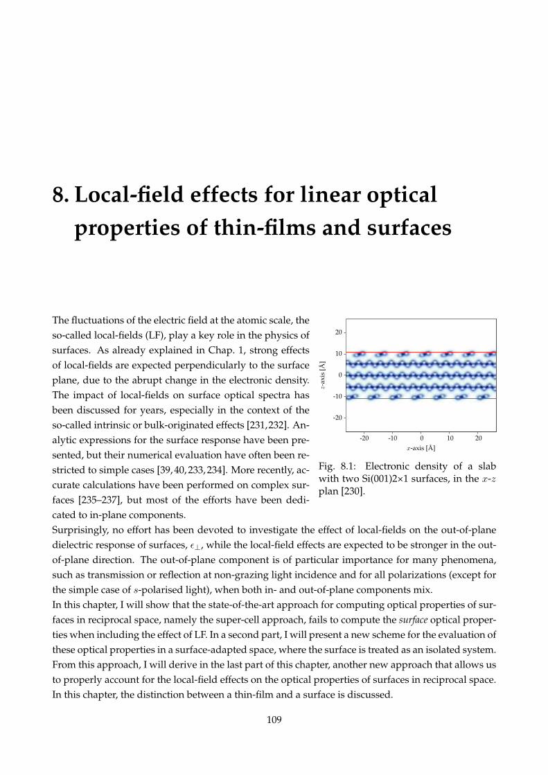
8. Local-field effects for linear opticalproperties of thin-films and surfaces
Fig. 8.1: Electronic density of a slabwith two Si(001)2×1 surfaces, in the x-zplan [230].
The fluctuations of the electric field at the atomic scale, theso-called local-fields (LF), play a key role in the physics ofsurfaces. As already explained in Chap. 1, strong effectsof local-fields are expected perpendicularly to the surfaceplane, due to the abrupt change in the electronic density.The impact of local-fields on surface optical spectra hasbeen discussed for years, especially in the context of theso-called intrinsic or bulk-originated effects [231,232]. An-alytic expressions for the surface response have been pre-sented, but their numerical evaluation have often been re-stricted to simple cases [39, 40, 233, 234]. More recently, ac-curate calculations have been performed on complex sur-faces [235–237], but most of the efforts have been dedi-cated to in-plane components.Surprisingly, no effort has been devoted to investigate the effect of local-fields on the out-of-planedielectric response of surfaces, ǫ⊥, while the local-field effects are expected to be stronger in the out-of-plane direction. The out-of-plane component is of particular importance for many phenomena,such as transmission or reflection at non-grazing light incidence and for all polarizations (except forthe simple case of s-polarised light), when both in- and out-of-plane components mix.In this chapter, I will show that the state-of-the-art approach for computing optical properties of sur-faces in reciprocal space, namely the super-cell approach, fails to compute the surface optical proper-ties when including the effect of LF. In a second part, I will present a new scheme for the evaluation ofthese optical properties in a surface-adapted space, where the surface is treated as an isolated system.From this approach, I will derive in the last part of this chapter, another new approach that allows usto properly account for the local-field effects on the optical properties of surfaces in reciprocal space.In this chapter, the distinction between a thin-film and a surface is discussed.
109
Chapter 8. Local-field effects for linear optical properties of thin-films and surfaces
8.1 Local-field effects and super-cells
In order to investigate the LF effects on optical properties of surfaces, we have chosen a slab with twoclean Si(001)2×1 surfaces as a model system. 1 The surface has been studied with the experimentallattice constant of 5.43 Å and N = 16 atomic layers (32 atoms), corresponding to a slab of thickness21.72 Å. Dielectric functions have been calculated using the TDDFT code DP [116].The optical dielectric function is given, in reciprocal space, by
ǫM (ω) = limq→0
1
ǫ−1G=G′=0(q;ω)
. (8.1)
Here q denotes a vanishing wave-vector and G, G′ are reciprocal lattice vectors of the crystal. The in-verse of the microscopic dielectric matrix is given by ǫ−1
GG′(q;ω) = δGG′ +v(q+G)χ(1)GG′(q;ω), where
v(q+G) = 4π/|q+G|2 is the Coulomb potential and χ(1) the density response function. In frequencyand reciprocal space, one has to solve a Dyson-like matrix equation for obtaining χ(1)
GG′(q;ω)
χ(1)GG′(q;ω) = χ
(1)0,GG′(q;ω) +
∑
G′′G′′′χ(1)0,GG′′(q;ω)KG′′G′′′(q;ω)χ
(1)G′′′G′(q;ω). (8.2)
In principle, the kernel K contains two terms, the Coulomb potential v and the exchange-correlationkernel fxc. In the following of this chapter, we will restrict ourselves to the Random-Phase Ap-proximation (RPA), where fxc = 0, as we are interested only in the description of the local-fields.Nevertheless, our results are general and can be used for any kernel. χ(1)
0 is the independent-particleresponse function given in reciprocal space by
χ(1)0,GG′(q;ω) =
2
NkVcell
∑
m,n
BZ∑
k
(fn,k − fm,k+q)〈n,k|e−i(q+G)r|m,k+ q〉〈m,k+ q|ei(q+G′)r|n,k〉
(En,k − Em,k+q + ω),
(8.3)where fn,k is the Fermi occupation number of the Bloch state |n,k〉 with the energy En,k. Nk is thenumber of k-points and Vcell refers to the volume of the cell, ω = ω + iη is the frequency with a smallpositive imaginary part η, that turns on adiabatically the electromagnetic field. The volume of thematter inside the cell is denoted Vmat in the following.
Param. void1 void2 void3
nkpt 256 256 256nband 300 300 400npwwfn 1499 1499 7987npwmat 299 391 399
Tab. 8.1: Parameters.
In Fig. 8.2, we present the results of the IPA calcu-lation, where ǫM = 1 − v0χ
(1)0,00, with χ
(1)0 defined by
Eq. (8.3), for different sizes of the vacuum slab, denotedvoid1 (vacuum size=21.72 Å; Vcell/Vmat = 2), void2 (vac-uum size=43.44 Å; Vcell/Vmat = 3) and void3 (vacuumsize=65.17 Å; Vcell/Vmat = 4), as schematically shown. Theconvergence parameters are given in Tab. 8.1. We presentalso the result of the renormalized super-cell calculation,using Vmat instead of Vcell for the normalization volume in Eq. (8.3). In that case, the result of the cal-
1This surface has already been presented in Chap. 4 and the numerical details such as atomic positions have been givenin Sec. 5.1.3.
110
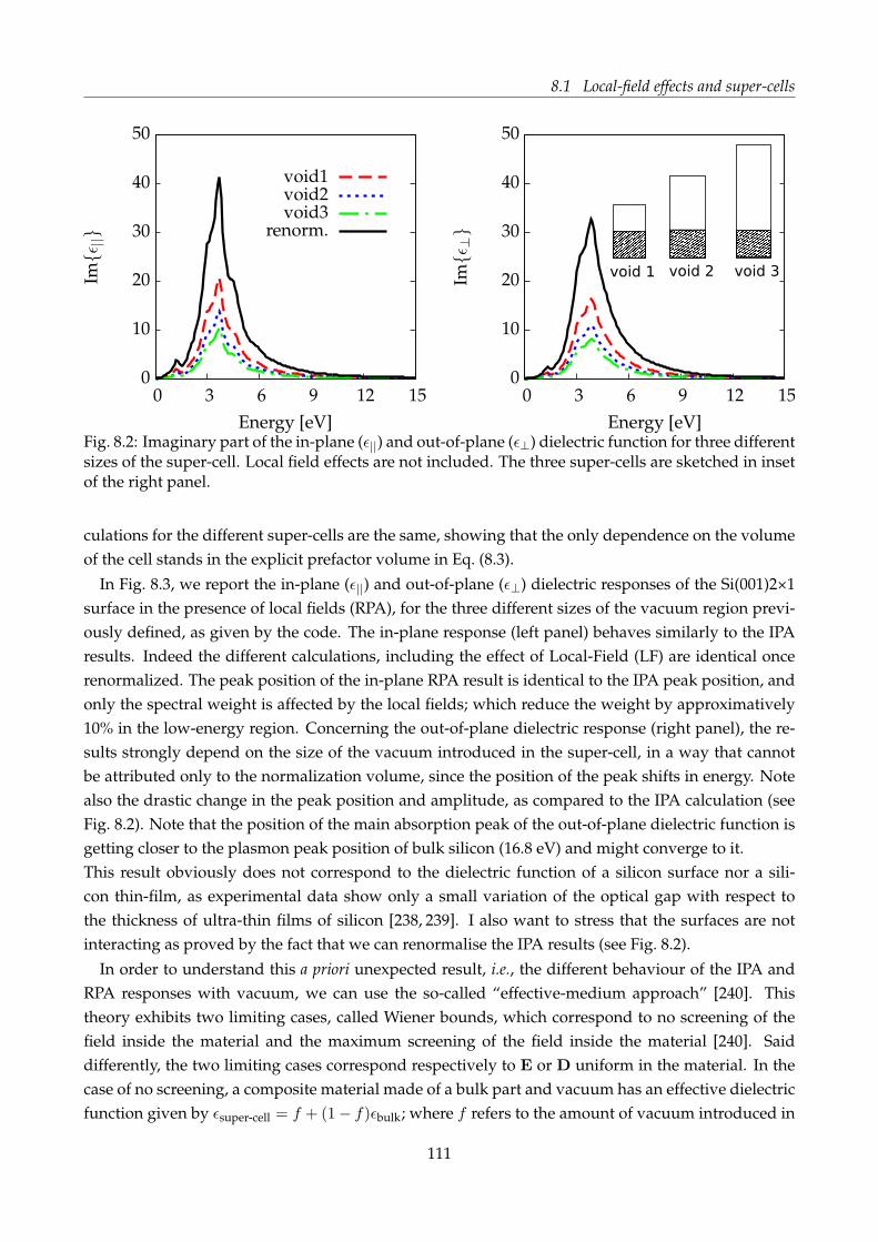
8.1 Local-field effects and super-cells
Fig. 8.2: Imaginary part of the in-plane (ǫ||) and out-of-plane (ǫ⊥) dielectric function for three differentsizes of the super-cell. Local field effects are not included. The three super-cells are sketched in insetof the right panel.
culations for the different super-cells are the same, showing that the only dependence on the volumeof the cell stands in the explicit prefactor volume in Eq. (8.3).
In Fig. 8.3, we report the in-plane (ǫ||) and out-of-plane (ǫ⊥) dielectric responses of the Si(001)2×1surface in the presence of local fields (RPA), for the three different sizes of the vacuum region previ-ously defined, as given by the code. The in-plane response (left panel) behaves similarly to the IPAresults. Indeed the different calculations, including the effect of Local-Field (LF) are identical oncerenormalized. The peak position of the in-plane RPA result is identical to the IPA peak position, andonly the spectral weight is affected by the local fields; which reduce the weight by approximatively10% in the low-energy region. Concerning the out-of-plane dielectric response (right panel), the re-sults strongly depend on the size of the vacuum introduced in the super-cell, in a way that cannotbe attributed only to the normalization volume, since the position of the peak shifts in energy. Notealso the drastic change in the peak position and amplitude, as compared to the IPA calculation (seeFig. 8.2). Note that the position of the main absorption peak of the out-of-plane dielectric function isgetting closer to the plasmon peak position of bulk silicon (16.8 eV) and might converge to it.This result obviously does not correspond to the dielectric function of a silicon surface nor a sili-con thin-film, as experimental data show only a small variation of the optical gap with respect tothe thickness of ultra-thin films of silicon [238, 239]. I also want to stress that the surfaces are notinteracting as proved by the fact that we can renormalise the IPA results (see Fig. 8.2).
In order to understand this a priori unexpected result, i.e., the different behaviour of the IPA andRPA responses with vacuum, we can use the so-called “effective-medium approach” [240]. Thistheory exhibits two limiting cases, called Wiener bounds, which correspond to no screening of thefield inside the material and the maximum screening of the field inside the material [240]. Saiddifferently, the two limiting cases correspond respectively to E or D uniform in the material. In thecase of no screening, a composite material made of a bulk part and vacuum has an effective dielectricfunction given by ǫsuper-cell = f + (1− f)ǫbulk; where f refers to the amount of vacuum introduced in
111

Chapter 8. Local-field effects for linear optical properties of thin-films and surfaces
Fig. 8.3: Imaginary part of the in-plane (ǫ||) and out-of-plane (ǫ⊥) dielectric function for three differentsizes of the super-cell. Local field effects are included. Note the change in the scale for the right panel.
the composite. This case corresponds to the case of the independent-particle approximation as thereis no local-fields, thus explaining why all the spectra (in-plane and out-of-plane) behave similarlywith vacuum.
Fig. 8.4: Comparison between the super-celland effective medium theory calculations.
In the case of the in-plane RPA optical responses,there is almost no local-field effects, because we areclose to the no-screening case, and the correspondingformula is valid. In the out-of-plane direction, whenlocal-field effects are included, the correct descriptionusing the effective-medium theory is the maximalscreening limit. I show in Fig. 8.4 the results obtainedthrough the effective-medium approach for maximalscreening, i.e., using ǫ−1
super-cell = f + (1 − f)ǫ−1bulk, ap-
plied to the super-cells and compared to the out-of-plane result of Fig. 8.3.This simple model reproduces quite well the TDDFTresults and thus shows that the standard calculationin a super-cell approach amounts to averaging overthe whole super-cell. The conclusion of this comparison is that when using super-cells in reciprocalspace, only the optical properties of the entire super-cell, as an effective medium, are obtained; andthe optical response of the slab is not accessible directly.Notice that some failures of the super-cell approach have already been pointed out, e.g., in Ref. [241],where authors have noticed that the screened Coulomb interaction W is “substantially influenced bythe repeated-slab geometry”.
112
8.2 Mixed-space approach
8.2 Mixed-space approach
8.2.1 A surface-adapted space
The super-cell approach and the periodicity implied by this method is not perfectly adapted to theslab geometry. Indeed, the surfaces that we want to model are periodic systems in two dimensionsand aperiodic in the third one. Moreover, as shown above, the super-cells do not yield the expectedslab optical response.Therefore, I chose a different approach for computing optical properties of surfaces, changing tothe real space for computing the optical properties. The idea of abandoning the periodic boundaryconditions and to work in real-space is not a novel idea of this thesis, and was already suggested inRef. [241] as a possible cure for issues related to the super-cell approach. The authors decided to notinvestigate this approach in their paper. The real space approach for computing optical properties ofsurfaces has been successfully applied to surface plasmons, e.g., Refs. [242, 243].The surfaces are isolated in the out-of-plane direction. Thus, in the direction perpendicular to theplane of the surface, I decided to treat the system in real space, as it is known to be efficient forisolated systems. The in-plane directions are treated in the reciprocal space, as it is customary forextended systems. In this thesis, I refer to this space as the “mixed-space”.In this mixed-space, the slab is truly isolated, because there is no out-of-plane periodicity; whereasin reciprocal space, the slab is artificially isolated by increasing the size of the vacuum region. As aconsequence, we expect calculations in the mixed-space to yield directly the optical properties of theslab and not of the super-cell. Also, in the mixed-space, the size of the vacuum region is no morea convergence parameter and the vacuum serves only for describing the exponential decay of thedensity.At the light of all these points, the mixed-space appears as the natural choice for working with thin-films and surfaces. Nevertheless, as it will be discussed latter, the numerical cost associated withthe mixed-space is prohibitive and a new approach, also developed during this thesis should bepreferred instead.
8.2.2 TDDFT and mixed-space in practice
Let us consider a super-cell containing a slab of matter and some vacuum. We denote the height ofthis super-cell Lz whereas Lmat
z refers to the thickness of the slab. The calculation of optical propertiesof surfaces in the mixed-space proceeds as follow:
1. The independent-particle susceptibility χ(1)0 (q||, z, z
′;ω) is computed. Instead of writing a newTDDFT code for computing the quantity χ(1)
0 (q||, z, z′;ω) directly, I obtained this quantity from
the DP code [116]. More precisely, χ(1)0 (q||, z, z
′;ω) is obtained by Fourier transforming the
matrix[
χ(1)0 (q;ω)
]
Gz ,G′z
, computed with the DP code. 2
2The initial super-cell represents a periodic system. Nevertheless, in real space, we pad the space with zeros, thusisolating the system. Therefore we describe an isolated slab, even if the initial IPA response function has been calculatedwith a super-cell approach.
113
Chapter 8. Local-field effects for linear optical properties of thin-films and surfaces
2. The fully interacting response function χ(1) is obtained by solving the Dyson-like equation.In Ref. [242], authors have shown that neglecting the in-plane dispersion of the susceptibilitygives reliable results for surface calculations. Under that approximation, i.e., considering onlythe components of the response functions such as G|| = G′
|| = 0 as in-plane reciprocal latticevectors, the Dyson-like equation reads as3
χ(1)(q||, z, z′;ω) = χ
(1)0 (q||, z, z
′;ω) +∫ +∞
−∞dz1dz2χ
(1)0 (q||, z, z1;ω)v(q||, z1, z2)χ
(1)(q||, z2, z′;ω).
(8.4)In practice, this equation is solved on a real space grid. On a grid, the Dyson equation Eq. (8.4)becomes a matrix equation. The solution of this matrix equation reads as
χ(1)(q||;ω) =1
∆zM−1(q||;ω)χ
(1)0 (q||;ω), (8.5)
where M(q||;ω) is an NG ×NG matrix defined by
Mij(q||;ω) =M(q||, zi, zj ;ω) =δij∆z
−∑
k
χ(1)0 (q||, zi, zk;ω)v(q||, zk, zj)∆z,
with the 2D Fourier transform of the Coulomb potential given by
v(q||, z, z′) = 2πe−|q||||z−z′|/|q|||. (8.6)
3. In order to compute the absorption spectra, the inverse of the microscopic dielectric matrix,defined by [244, 245]
ǫ−1(q||, z, z′;ω) = δ(z, z′) +
∫
dz1v(q||, z, z1)χ(1)(q||, z1, z
′;ω)
grid≈ δij∆z
+∑
zk
v(q||, zi, zk)χ(1)(q||, zk, zj ;ω)∆z, (8.7)
is averaged, using
ǫ−1(q;ω) =1
Lz
∫
dz
∫
dz′e−iqzzǫ−1(q||, z, z′;ω)eiqzz
′ grid≈∑
zi,zj
e−iqz(zi−zj)ǫ−1(q||, zi, zj ;ω)∆2
z
Lz.
(8.8)Notice here that this is the macroscopic average [44] which is computed, i.e., containing the fulldependence on the momentum q, and not a spatial average which would contain only the in-plane momentum. This allows us to compute all the components of the dielectric tensor, asexplained below, and also to compare with previous results for instance.
3The approximation of taking only the G|| = G′|| = 0 contribution reduces drastically the burden associated with the
solution of this equation, and is enough as we are using the real space approach as a test-case.
114

8.2 Mixed-space approach
4. The macroscopic dielectric tensor is computed, using the usual expression
ǫM (q;ω) = limq→0
1
ǫ−1(q;ω).
Due to the expression of the Coulomb potential in the mixed-space Eq. (8.6), some care is requiredfor computing the zz component of the macroscopic dielectric tensor. Indeed, for obtaining the zzcomponent, one would choose q = qzez. But this leads to a divergent Coulomb potential (see Eq.(8.6))which is prohibited for numerical simulations. This can be disappointing considering that I decidedto use the mixed-space method precisely to calculate the out-of-plane component of the dielectrictensor.This apparent problem is nevertheless solved easily using the following approach:i) The non-interacting response function χ
(1)0 is evaluated for three different values of q, which are
q1 = q||ex, q2 = q||ex + qzez and q3 = q||ex − qzez.ii) The macroscopic dielectric tensor ǫ(q1;ω) = ǫxx(ω), ǫ(q2;ω) and ǫ(q3;ω) are computed accordingto the mixed-space scheme, as already explained.iii) From simple algebra, using the tensorial nature of the dielectric tensor, one obtains that
ǫxz(ω) =1
4ab
(
ǫ(q2;ω)− ǫ(q3;ω))
,
ǫzz(ω) =1
b2
(
ǫ(q2;ω)− a2ǫxx(ω)− 2abǫxz(ω))
,
where a =q||
√
q2||+q2zand b = qz
√
q2||+q2z.
Some care is required in order to choose the values of q|| and qz . As we are interested in the opticalproperties, we assume the optical limit; which constrains us to the limit q → 0. To avoid numericalproblems, we want to have non-vanishing values of q|| and qz , in order to have reliable numeri-cal results when evaluating ǫzz(ω). It is possible to satisfy these two constrains, remembering thatthe χ(1)
0 (q,q;ω) is analytically proportional to |q|2 in the optical limit. Also the matrix elementsχ(1)0 (q,q + G;ω) and χ
(1)0 (q + G,q;ω) are proportional to |q|, G 6= 0. The same holds for χ(1) [54].
Therefore, when calculating the matrix χ(1)0 with the DP code, a vanishing value of q is used. Then,
before performing the Fourier transform for obtaining χ(1)0 (q||, zi, zj ;ω), the aforementioned matrix
elements are rescaled, in order to have q||, qz ∼ 1.
8.2.3 Numerical results
During this thesis, I have implemented this numerical scheme using the software MATLAB [246].In Fig. 8.5, I report the numerical results, obtained using the mixed-space scheme, for the cleanSi(001)2×1 surface. I used 1400 Gz-vectors, corresponding to a spacing of ∆z = 0.0635 Å, in or-der to reach convergence. We checked that the RPA results are independent of the size of the vacuumregion used in the super-cell, as expected for a mixed-space calculation. The striking point is theweak effect of local-fields on Imǫ⊥, in comparison to the previous results, presented on the rightpanel of Fig. 8.3. Also we obtain no effect of LF on the in-plane component (Fig. 8.3; left panel) ofthe dielectric tensor. Indeed, the peak positions and intensities are identical to the IPA calculation.
115
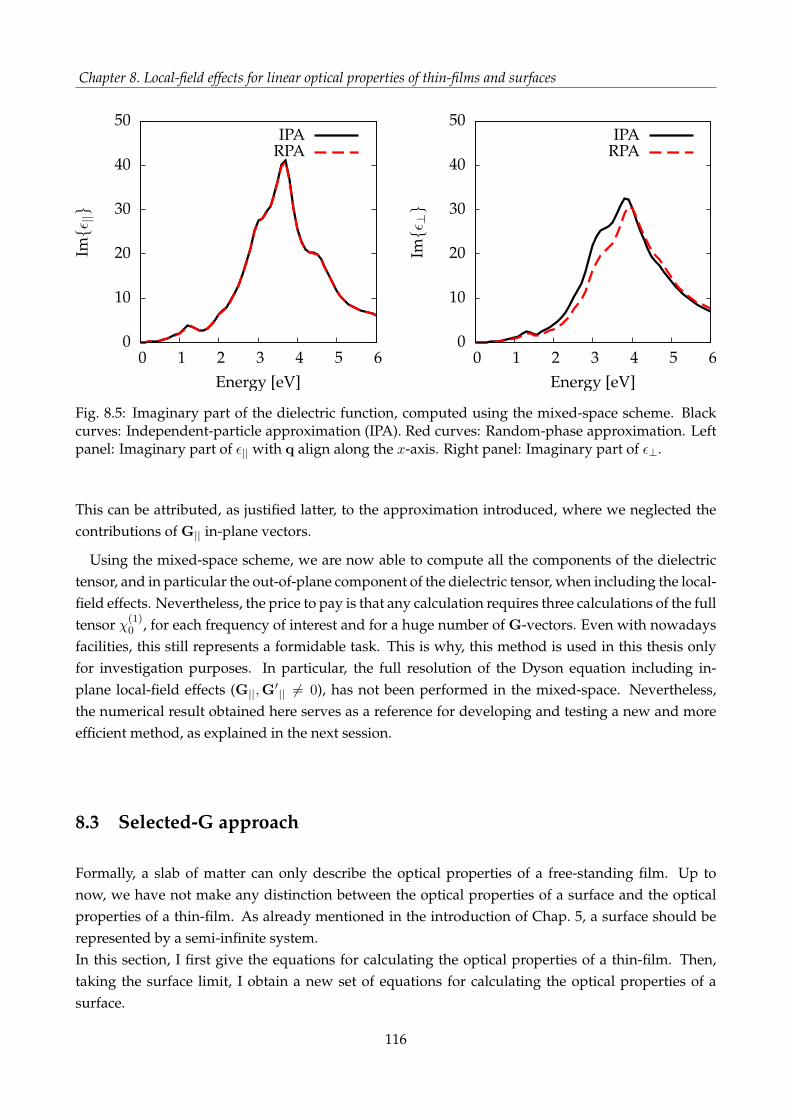
Chapter 8. Local-field effects for linear optical properties of thin-films and surfaces
Fig. 8.5: Imaginary part of the dielectric function, computed using the mixed-space scheme. Blackcurves: Independent-particle approximation (IPA). Red curves: Random-phase approximation. Leftpanel: Imaginary part of ǫ|| with q align along the x-axis. Right panel: Imaginary part of ǫ⊥.
This can be attributed, as justified latter, to the approximation introduced, where we neglected thecontributions of G|| in-plane vectors.
Using the mixed-space scheme, we are now able to compute all the components of the dielectrictensor, and in particular the out-of-plane component of the dielectric tensor, when including the local-field effects. Nevertheless, the price to pay is that any calculation requires three calculations of the fulltensor χ(1)
0 , for each frequency of interest and for a huge number of G-vectors. Even with nowadaysfacilities, this still represents a formidable task. This is why, this method is used in this thesis onlyfor investigation purposes. In particular, the full resolution of the Dyson equation including in-plane local-field effects (G||,G
′|| 6= 0), has not been performed in the mixed-space. Nevertheless,
the numerical result obtained here serves as a reference for developing and testing a new and moreefficient method, as explained in the next session.
8.3 Selected-G approach
Formally, a slab of matter can only describe the optical properties of a free-standing film. Up tonow, we have not make any distinction between the optical properties of a surface and the opticalproperties of a thin-film. As already mentioned in the introduction of Chap. 5, a surface should berepresented by a semi-infinite system.In this section, I first give the equations for calculating the optical properties of a thin-film. Then,taking the surface limit, I obtain a new set of equations for calculating the optical properties of asurface.
116
8.3 Selected-G approach
8.3.1 Isolated system from periodic super-cell calculations
From the previous results, it is clear now that the periodicity induced by the super-cell approach,treated in reciprocal space, is at the origin of the failure of the super-cell approach. We must treata thin-film as an isolated system in the out-of-plane direction in order to properly include the local-field effects in its optical properties.Let us consider such an isolated thin-film. We introduce the following approximation: the matter,i.e., the density, is localised in the z-direction between −Lmat
z and 0. This is justify by the observationof the density of silicon slabs, as shown in Fig. 8.1. The full space has an extension in the z-direction,denoted Lz , with Lz → ∞.
Considering that response functions are restricted to the matter region, the full Dyson equation,expressed in the mixed-space, reads as
χ(1)G||G′||
(q||, z, z′;ω) = χ
(1)0,G||G′||
(q||, z, z′;ω) +
∑
G1||
∫ 0
−Lmatz
dz1dz2χ(1)0,G||G1||
(q||, z, z1;ω)
× vG1||(q||, z1, z2)χ(1)G1||G′||
(q||, z2, z′;ω), z, z′ ∈ [−Lmat
z , 0].
(8.10)
In contrast to Eq. (8.4), we consider here the full dependence on the in-plane G-vectors.Instead of solving this equation directly in the mixed-space, as already done in the previous section,we introduce here two auxiliary functions χ(1)
0 and χ(1). These functions are respectively identical toχ(1)0 and χ(1) for (z, z′) ∈ [−Lmat
z , 0] × [−Lmatz , 0]. These functions are also chosen periodic, of period
Lmatz
4
χ(1)0,G||G′||
(q||, z +NLmatz , z′ +NLmat
z ;ω) = χ(1)0,G||G′||
(q||, z, z′;ω),
χ(1)G||G′||
(q||, z +NLmatz , z′ +NLmat
z ;ω) = χ(1)G||G′||
(q||, z, z′;ω).
N ∈ Z
Note that in the standard super-cell calculations, the response functions have a periodicity of Lz in-stead of the periodicity of Lmat
z that we have here for the auxiliary response functions. These auxiliaryresponse functions being periodic, it is possible to define their (inverse) Fourier transform
χG,G′(q;ω) =
1
Lmatz
∫ 0
−Lmatz
dz
∫ 0
−Lmatz
dz′e−i(qz+Gz)zχG||,G′||(q||, z, z′;ω)ei(qz+G′
z)z′, (8.11a)
χG||,G′||(q||, z, z′;ω) =
1
Lmatz
∑
qz
∑
Gz ,G′z
ei(qz+Gz)zχG,G′(q;ω)e
−i(qz+G′z)z
′, z, z′ ∈ [−Lmat
z , 0], (8.11b)
with Gz = N 2πLmatz
, N ∈ Z.
4The remaining space is filled with zero.
117
Chapter 8. Local-field effects for linear optical properties of thin-films and surfaces
Dyson-like equation
Using Fourier transform definitions, together with definition of delta functions (see App. A), weobtain a Dyson-like equation for the auxiliary response function χ(1)
χ(1)
GG′(q;ω) = χ(1)
0,GG′(q;ω) +1
Lmatz
∑
G1||
∑
Gz1Gz2
χ(1)0,G||G1||
(q||, qz + Gz, qz + Gz1;ω)
×∫ 0
−Lmatz
dz1dz2
(
e−i(qz+Gz1)z1vG1||(q||, z1, z2)ei(qz+Gz2)z2
)
χ(1)G1||G′||
(q||, qz + Gz2, qz + G′z;ω).
(8.12)
This equation can be written in a more compact way
χ(1)
GG′(q;ω) = χ(1)
0,GG′(q;ω) +∑
G1G2
χ(1)
0,GG1(q;ω)v
G1G2(q)χ
(1)
G2G′(q;ω), (8.13)
by defining
vG1,G2
(q) =1
Lmatz
∫ 0
−Lmatz
dz1
∫ 0
−Lmatz
dz2e−i(qz+Gz1)z1vG1||(q||, z1, z2)e
i(qz+Gz2)z1δG1||,G2|| . (8.14)
Using the expression of the Coulomb potential, it is possible to obtain a simplified analytical expres-sion of v
G1,G2(q), as shown in App. G.
Dielectric response
The inverse dielectric function is given by
ǫ−1(q||, z, z′;ω) = δ(z, z′) +
∫
dz1v(q||, z, z1)χ(1)(q||, z1, z
′;ω)
= δ(z, z′) +∫ 0
−Lmatz
dz1v(q||, z, z1)χ(1)(q||, z1, z
′;ω),(8.15)
where the last equation comes from the approximation that response functions are restricted to[−Lmat
z , 0]× [−Lmatz , 0].
The macroscopic average of the inverse dielectric function Eq. (8.8), averaged over the slab, reads as
ǫ−1(q;ω) =1
Lmatz
∫ 0
−Lmatz
dz
∫ 0
−Lmatz
dz′e−iqzzǫ−1(q||, z, z′;ω)eiqzz
′
= 1 +∑
q′zGzG′z
v0Gz
(q||, qz)χ(1)
GzG′z
(q||, q′z;ω)e
−i(q′z−qz+G′z)
Lmatz2 sinc([q′z − qz + G′
z]Lmatz
2).
(8.16)As a result, we obtain that in order to compute the optical properties of an isolated thin-film inreciprocal space, we have to proceed in two steps. First, the Dyson equation Eq. (8.13), which links thefully interacting response function χ(1) to the independent-particle response function χ(1)
0 is solved.In this equation, the Coulomb potential v is replaced by a modified Coulomb potential v, given byEq. (8.14) or equally by Eq. (G.5). Then, the dielectric response of the thin-film is computed, according
118

8.3 Selected-G approach
to Eq. (8.16). Again, this definition contains the modified Coulomb potential v. It is important tonote that this modified Coulomb potential v is not diagonal in reciprocal space and has a complexanalytical expression (see App. G), making the resolution of the Dyson equation Eq. (8.13) moreintricate.
8.3.2 Selected-G approach
In order to describe the optical properties of a surface from a thin-film of thickness Lmatz , we must
take the limit Lmatz → ∞. I refer to this limit as the surface limit.
As shown in App. G, within the surface limit,
vG1,G2
(q) =4π
|q+ G|2δG1,G2
= vG1
(q)δG1,G2
, (8.17)
where v is the Coulomb potential. Inserting this result in Eq. (8.13) and Eq. (8.16) gives a new set ofequations
χ(1)
GG′(q;ω) = χ(1)
0,GG′(q;ω) +∑
G1
χ(1)
0,GG1(q;ω)v
G1(q)χ
(1)
G1G′(q;ω),
ǫ−1(q;ω) = 1 + v0(q)χ(1)00 (q;ω).
(8.18a)
(8.18b)
These two equations are very similar to the usual equations of the TDDFT. Only the definition ofthe G-vectors involved in is different. The equation Eq. (8.18a) contains the G-vectors correspondingto the material slab volume.
Fig. 8.6: Selected-G method for Lz = 2Lmatz .
If we now choose the vacuum region to be an in-teger multiple of the height of the material slab, weobtain an easy way to construct the matrix χ(1)
0 fromχ(1)0 . Indeed, in this case, the matrix elements of χ(1)
0
are matrix elements of χ(1)0 . Thus χ(1)
0 is obtainedby keeping only matrix elements of χ(1)
0 given by thesubset of the super-cell’sGz-vectors corresponding toGz-vectors of the material slab; and by replacing thevolume of normalisation Vcell in Eq. (8.3) by the vol-ume of matter Vmat, accordingly to the definition ofthe Fourier transform Eq. (8.11a).
8.3.3 Numerical results
I have implemented the Selected-G approach in the DP code. The same parameters (see Tab. 8.1) havebeen used to obtain the spectra. In particular, 299 G-vectors have been used in total, i.e., includingin-plane and out-of-plane G-vectors. This is to be compared with the 1400 Gz-vectors needed forthe mixed-space original scheme, where the in-plane dispersion is neglected. The result of this newframework, called ”Selected G“ is presented in Fig. 8.7 (red dashed line).In the inset, we checked that solving the Dyson equation Eq. (8.18a) with slab’sGz , but keeping G|| =
119

Chapter 8. Local-field effects for linear optical properties of thin-films and surfaces
Fig. 8.7: Imaginary part of the dielectric function ǫ|| with q aligned along the x-axis (left panel) andǫ⊥ (right panel). Black solid curves: Independent-particle approximation (IPA). Red dashed curves:Mixed-space calculation. Blue dotted curves: Selected-G calculation. Inset: Comparison betweenthe mixed-space and the Selected-G method, without in-plane reciprocal vectors (”Gz-only“, greendotted-dashed curve).
0, gives the same results as the mixed-space approach. The error introduced by the approximation ofthe strict localisation of response function between −Lmat
z and 0 is negligible and appears a posteriori
as a good and perfectly valid approximation. The differences with the mixed-space calculationsoriginate then from the approximation introduced in this last approach. This allows us to understandhow local fields built in, in terms of G|| and Gz .
Fig. 8.8: Imaginary part of the dielectric re-sponses of the surface and the bulk, localfields included.
It appears that ǫ⊥ depends on both G|| and Gz
(right panel: blue and red curves). On the contrary,as shown in the left panel, ǫ|| is only influenced byG||, as the curves labelled ”IPA“ and ”Mixed-space“are superposed. We also observe that the weak de-pendence of ǫ|| on Gz explains why the standard ap-proach leads to a correct description of the local fieldsin the plane of the surface, although the set of Gz is notadapted to the material slab. We do not show the re-sults for several sizes of the vacuum region as theyare indistinguishable.These results allow us to discuss for the first time theeffect of the local-fields on the different componentsof the optical dielectric function for a surface.We compare in Fig. 8.8 the imaginary part of ǫ⊥, ǫxx||and ǫyy|| for the clean Si(001)2×1 surface to the absorp-tion spectra silicon bulk, including local-fields in all cases.The main effect is a blue shift of approximately 0.3 eV in the position of the peak for ǫ⊥, compared to
120

8.4 Discussion
the bulk response, while no shift is observed for ǫ||. The decrease in the intensity of the main absorp-tion peak is more pronounced for ǫ⊥ than for ǫ||. This effect was already visible in the IPA calculation(see Fig. 8.2) and for this reason, it can be attributed to the presence of the surface itself, and not tothe local-fields.For the clean Si(001)2×1 surface, the atomic relaxation at the interface with vacuum introduces states,located in the gap of the material, the so-called surface-states, which are evidenced in the IPA cal-culation by the appearance of a small structure around 1.3 eV, see the black curve in Fig. 8.7. Withlocal-fields included, this structure is still clearly visible in ǫ||, in particular for ǫyy|| (see Fig. 8.8). Inthe case of ǫ⊥, the peak vanishes when all the G|| and Gz are taken into account, while it remains,in the mixed-space calculation, including the Gz only, evidencing the influence of the in-plane localfields (G|| 6= 0). This also shows how local-field effects are important for the correct description ofsurface-induced structures.
8.4 Discussion
8.4.1 Independence of the two surfaces in a slab geometry
The two surfaces of a slab have been shown to be independent in Chap. 5, in the independent-particleapproximation. Here I check the independence of the two surfaces of a slab when local-field effectsare included. Due to the Coulomb interaction, which is a long-range interaction, the two surfaces ofa slab of matter may potentially couple. In that case, it would not be possible to map the result of acalculation performed using a slab geometry to the semi-infinite system that we try to model, eventaking the surface limit (Lmat
z → ∞).Let us consider the spectra of two symmetric slabs, one with two clean surfaces and one with two
dihydride surfaces. If the surfaces of a slab are independent, the average of these two symmetricspectra should be identical to the spectrum of an asymmetric slab, with a front clean surface and aback dihydride surface, as depicted in Fig. 5.3. Calculations of these three slabs have been performedusing the Selected-G method, including the local-field effects. The spectra have been computed fortwo different slab sizes; 12 atomic layers (top panels) and 16 atomic layers (bottom panels). Resultsare presented in Fig. 8.9.The differences between the average (”Average“) and the asymmetric slab (”Clean-DiH“) are foundto be small for the 12 atomic layers. When increasing the thickness of the slab, the differences almostvanish, showing that the surfaces become independent. I checked that the IPA results yield the samequantitative differences. Therefore these differences do not originate from the Coulomb interactionbut from the size of the slab. This shows that the surfaces are numerically independent when includ-ing local-field effects.Note that by comparing the density of a slab and the one of bulk silicon (see Sec. 5.2.6), I alreadyfound in Chap. 5.2.6 that the surface-states live in a ∼8.5Å wide region. The half-slab thicknessesare respectively here 8.15Å (”12 layers“) and 10.86Å (”16 layers“). This explains that when using aslab made of 12 atomic layers, the surface-states of each side of the slab slightly overlap, resulting insmall interferences. From these results, we obtain a condition of independence of the surfaces of theslabs, which is that the surface states of the two surfaces must not overlap. In the case of the clean
121

Chapter 8. Local-field effects for linear optical properties of thin-films and surfaces
Fig. 8.9: Comparison between the real part (left panel) and imaginary part (right panel) of ǫzz com-puted for the asymmetric slab (Clean-DiH; solid curve), a symmetric clean slab (Clean-Clean; bluedotted curve), a symmetric dihydride slab (DiH-DiH; green dotted dashed curve) and from the av-erage of the two symmetric slabs (Average; dashed curve). Local field effects are included.
surface, this imposes a slab to contain at least 16 layers.
8.4.2 Surface dielectric function and three-layer model
One must be careful when interpreting the optical spectra obtained from the Selected-G approach,especially the variation of the spectra with respect to the number of layers or atoms in the slab.Indeed, the position and amplitude of the surface spectra depend on the number of atomic layers inthe slab. This is well illustrated in Fig. 8.10. We observe in Fig. 8.10 that the slab calculations slowlyconverge to the bulk spectra when increasing the number of atoms. In order to show that we reallyconverge to the bulk spectra, I reported in Fig. 8.11 the evolution of the intensity of the E2 related
122

8.4 Discussion
Fig. 8.10: Imaginary part of the out-of-plane component of the dielectric tensor (ǫ||) versus the numberof layers in the slab, compared to the bulk silicon absorption spectra.
peak versus the number of layers (N ) in the slab. The value at zero correspond to the bulk case. Weclearly see that both IPA (black dots) and RPA (red dots) converge to the bulk values as 1/N .How to interpret and to extract information from these slab calculations is an intricate question.
It is common to use a three-layer model in order to extract surface quantities from a slab calcula-tion [247, 248]. In this model, the dielectric response of the slab is given by
ǫslabM (ω) =
(N − 2Ns)ǫbulkM (ω) + 2Nsǫ
surf(ω)
N, (8.19)
where N and Ns are respectively the total number of layers in the slab and the effective number ofsurface layers where the dielectric function equals the effective surface dielectric function ǫsurf(ω).There is (N − 2Ns) bulk layers with a dielectric function ǫbulk
M (ω). The factor 2 comes here from thefact that the slab has two surfaces.
Fig. 8.11: Convergence in number oflayers of the intensity of the E2 relatedpeak. Lines are here to guide the eyes.
Here we analyse the optical spectra obtained from theSelected-G method within the limits of this formula. Wechecked (not shown) that the surface optical region is fullycontained in the slab made of 20 atomic layers of matter,as we can extract the bulk absorption spectra from the slabcalculations performed with N = 20 layers and N = 24
layers.Thereby, it is possible to extract the surface-induced spec-tra using Eq. (8.19) from these slabs. More precisely, as it isnot possible to determine separately Ns and ǫsurf, we canonly determine the surface-induced quantityNs
(
ǫsurf(ω)−ǫbulkM (ω)
)
, which is the only meaningful physical quantitythat we can extract using Eq. (8.19).The quantityNs
(
ǫsurfyy (ω)−ǫbulk
M (ω))
has been extracted from the results of a 20 atomic layer slab (black
123

Chapter 8. Local-field effects for linear optical properties of thin-films and surfaces
Fig. 8.13: Spectra of Ns
(
ǫsurf(ω)− ǫbulkM (ω)
)
for the xx component (left panel) the yy component (mid-dle panel) and the zz components (right panel) for the clean surface. Dashed lines are obtainedwithout local-fields (”IPA“) whereas solid lines correspond to local-field effects included (”RPA“).The spectra is obtained from the 24 atomic layer slab.
lines) and a 24 atomic layers slab (red lines), as shown in Fig. 8.12. These two slabs yield the sameresult, showing the reliability of the approach.The same quantity is reported in Fig. 8.13, where the dashed lines are the results obtained withoutincluding the local-field effects (”IPA“) whereas the solid lines correspond to local-field included re-sults (”RPA“).We observe in Fig. 8.13 that the three different components of the dielectric tensor give quite differentresults. Nevertheless some features are common.
Fig. 8.12: Spectra ofNs
(
ǫsurfyy (ω)−ǫbulk
M (ω))
forthe clean surface, calculated for N = 20 lay-ers (black solid line) and N = 24 layers (reddashed line).
First, in all the spectra, there is a negative peakaround 3.7 eV (corresponding to the critical point E2
of bulk silicon) indicating a lowering of the intensityof this peak in the surface quantity. By opposition,all the spectra are positive between 0 eV and 2 eV,due to the presence of surface-states in the gap of theclean surface. The intensity of the E1 related peak isfound to be increased in the surface spectra for twoin-plane components of the dielectric tensor, whereasthe intensity of the same peak is reduced for the out-of-plane component. The xx component shows thesmallest deviation to the bulk spectra, as already vis-ible in Fig. 8.8.
The effects of the local fields are well evidenced inFig. 8.13. Indeed, on the xx and the zz components,the surface-states induced structures are reduced by the local-field effects, whereas the equivalentstructure on the yy component is unchanged when including local-field effects. Also the E2 relatedpeak intensity is closer to the bulk one when local-fields are included, for the in-plane components.For the out-of-plane components, the local-field effects induce a blue-shift of 0.1eV, whose conse-
124

8.4 Discussion
quence is to increase the difference at the energy position of the E2 critical point of bulk silicon.We note that the local-field effects do not change too much the spectral shape of the quantityNs
(
ǫsurf(ω) − ǫbulkM (ω)
)
, and more importantly, they do not change its sign. This means that whenthe surface quantity is smaller (bigger) in intensity than the bulk one, this remains true when in-cluding local-field effects. Finally, the prominent peak positions are found not to be affected by thelocal-field effects, expect a small blue-shift for the E2 peak of the zz surface optical response. Thismeans that the apparent blue-shift observed in Fig. 8.10 is mainly due to a change in the relativeweight between the ”surface“ spectra and the bulk one.
Conclusion
In summary, I have investigated in this chapter the local-field effects on the linear optical propertiesof surfaces. The standard reciprocal-space based super-cell approach, has been shown to only yieldthe optical properties of an effective medium matter plus vacuum and to fail in the out-of-planedirection. In order to compute the optical properties of the surface and not the super-cell, I have in-troduced two new efficient schemes to account for local-fields in the ab initio description of the opticalproperties of surfaces, for both parallel and perpendicular components.The two schemes are based on the resolution of TDDFT plus linear response theory equations in amixed-space designed to be adapted to the special periodicity of the slab geometry. The first schemecorresponds to the resolution of the equations in this mixed-space directly. This approach works per-fectly but an approximation has to be introduced to reduce the numerical cost of the calculation.In order to do better, I have derived from the mixed-space equations a second scheme, still based onthe super-cell approach, but which uses a selected set of reciprocal vectors. This scheme combinesthe correctness of the mixed-space approach, with the efficiency of a treatment in reciprocal space.Thanks to the efficiency of this scheme, we have been able to fully account for the local-field effects,removing the approximation introduced in the first scheme.We have then demonstrated how local-field effects are important for a correct description of the out-of-plane optical properties. Comparing the two schemes, I have explained how the local-field effectsconstruct, in terms of in-plane and out-of-plane G-vectors. In addition, it explains why the standardcalculation leads to reliable results for the in-plane components, as expected from the excellent agree-ment between theoretical and experimental results for Reflectance Anisotropy Spectra found in theliterature.Finally, I have checked that the two surfaces of a slab are independent, even including local-field ef-fects, and we have extracted the surface-induced modification to the bulk spectra assuming a three-layer model.In next chapter, I present the local-field effects for surface SHG, merging the extraction of the spectra(Chap. 5, Chap. 6 and Chap. 7) with the Selected-G approach for the calculation of local-field effects.
125


Part IV
Application to Silicon Surfaces
127

9. Local-field effects on second-harmonicgeneration from surfaces
The abrupt change in the electronic density at the surface of a dielectric mate-rial leads to a huge variation of the electric field at the interface with vacuum.As a result, strong effects of the local-fields on the optical properties of sur-faces are expected; in particular in the direction perpendicular to the plane ofthe surface. Therefore we except the local-field effects to affect quantitativelythe surface second-harmonic generation.It is still common practice to neglect local-field effects on surface second-harmonic generation spectra,and their effects have, so far, only been estimated using models fitted on experimental data [249,250].Understanding, by means of ab initio methods, how local-field effects affect the second-harmonic gen-eration (SHG) at crystal surfaces is the aim of this chapter.I report here a method of calculating the local-field effects in the Time-Dependent Density FunctionalTheory (TDDFT) framework, based on the macroscopic theory developed in Chap. 7. This macro-scopic theory is used to calculate the surface second-harmonic generation of some silicon surfacesand to investigate the effect of local-fields.The SHG from silicon surfaces has been widely studied in the literature [28, 78–80, 227, 251]; and itis found experimentally a strong influence of ad-atoms on the SHG spectra of silicon surfaces. Inparticular, the presence of hydrogen results in a quenching of the SHG signal [32, 33, 252–254]. Here,the local-field effects are investigated on the clean Si(001)2×1 surface, but also on two hydrogenatedsurfaces, namely the monohydride or Si(001)2×1:H and the dihydride or Si(001)1×1:2H surfaces; inorder to shed some light on the close connection between the surface SHG, the ad-atoms and thelocal-field effects.This chapter is organised as follow. First, I present the numerical results obtained at various lev-els of approximation, evidencing the role and the effects of the local-fields on the SHG spectra ofthe clean Si(001) surface. Then, the results obtained for two hydrogenated surfaces are presentedand compared with available data, evidencing the importance of local-field effects for a quantitativedescription of surface SHG.
129

Chapter 9. Local-field effects on second-harmonic generation from surfaces
9.1 Local-Field Effects on the clean Si(001) SHG spectra
9.1.1 Numerical implementation
I have implemented the expressions of the χ(0)Sρρ and χ
(0)Sρρρ , as well as the Selected-G method in
the SHG-TDDFT code known as 2light [117]. For conciseness, the expression of the full matrices[
χ(0)Sρρ
]
GG′ and[
χ(0)Sρρρ
]
GG′G′′ are derived and reported in App. I. Due to the impressive time re-quired for computed the entire matrix χ(0)S
ρρρ , I have modified the parallelization of the code from anOpenMP parallelization to an hybrid OpenMP+MPI parallelization. Thanks to some optimizationsof the 2light code, and to this new parallelization, I have been able to perform the calculations of sur-face second-harmonic generation on systems of reasonably converged size, fully taking into accountlocal-field effects.
9.1.2 Numerical details
Param. Value
nkpt 256npwwfn 3989nband 220lomo 40npwmat 93η 100 meV∆ω 100 meV
Tab. 9.1: Parametersfor the clean Si(001)2×1surface.
The self-consistent ground-state and the Kohn-Sham states were calculatedusing the plane-wave ABINIT code [115]. I used Troullier-Martins pseu-dopotentials [216] that are fully separable nonlocal pseudopotentials in theKleinman-Bylander form [120] for Si and H atoms. The contribution of thenonlocal part of the pseudo-potential to v and V is carried out using the2light code [117].The parameters of the atomic relaxation, as well as the values obtained forthe dimer bond-length and buckling are the same as in Sec. 5.1.3. The con-vergence in number of atoms is an important issue, but the calculation ofthe local-field effects requires the evaluation of the entire matrix χ(0)S
ρρρ for abig number of G-vectors, typically around 75-100. I found 24 atomic layersfor representing the full slab to give a good trade off between quantitativeresults and the numerical burden associated with the inclusion of local-field effects on the surfaceSHG spectra.
Fig. 9.1: SHG spectra |χ(2)S0,xxx| of the
clean surface calculated. The differentcurves are explained in the text.
For this slab made of 24 atomic layers, I found the con-verged parameters, which are reported in Tab. 9.1 for theclean Si(001) surface. The parameter “lomo” correspondsto the index of the first valence band included in the cal-culation. This parameter is quite important for optimizingthe computing time, as the computation of χ(0)S
ρρρ scales asN3
b , Nb being the number of bands considered in the sim-ulation. Fig. 9.1 shows the effect of choosing 40 as a valuefor the lomo parameters (“lomo 40”; black solid line), in-stead of taking all the valence bands (“lomo 1”; red dottedline). As the two spectra are almost indistinguishable, weuse for lomo the value of 40 in the following for the cleansurface, thus almost dividing by two the number of transitions to be computed.
130


Chapter 9. Local-field effects on second-harmonic generation from surfaces
Fig. 9.3: Comparison of the effect of scissors correction on the surface second-harmonic generationof the clean Si(001)2×1 surface, with (blue curves) and without (red curves) local fields included. Thescissors correction is chosen to be ∆ = 0.6eV . Arrows are here for indicating the positions of mainstructures.
∆/2 = 0.3eV (indicating their 2ω origin) whereas the two main structures in RPA are shifted by∆ = 0.6eV (indicating their 1ω origin). Therefore the main effect of local-fields on the zzz componentis not a blue shift but a redistribution of the spectral weight between the 2ω and the 1ω transitions.Concerning the yyz components, the LF do not alter the position of the prominent peaks, but they doreduce the spectral-weight of the main structures.
9.2 Hydrogenated surfaces and local-field effects
Param. DiH MonoH
nkpt 288 256npwwfn 3999 3989nband 140 220lomo 20 30npwmat 73 89η 100 meV∆ω 100 meV
Tab. 9.2: Parameters for thehydrogenated surface.
As explained in Chap. 4, it is possible to cover the Si(001) with ad-atoms and in particular with hydrogen atoms. The effect of the hy-drogen on the second-harmonic generation from silicon surfaces hasbeen widely investigated experimentally [32, 33, 252–254]; but theorigin of the hydrogen-induced quenching is not well understood.In this section, I report the effects of local-fields on the spectra of twohydrogenated surfaces, the monohydride Si(001)2×1:H and the di-hydride Si(001)1×1:2H surfaces.The parameters for these calculations are given in Tab. 9.2, re-spectively for the dihydride (“DiH”) and for the monohydride(“MonoH”) surfaces. Note that due to the symmetries of the dihy-dride surface, twice less atoms are needed to describe the surface;lowering the requirements in terms of number of bands, and thus reducing the numerical cost of
132

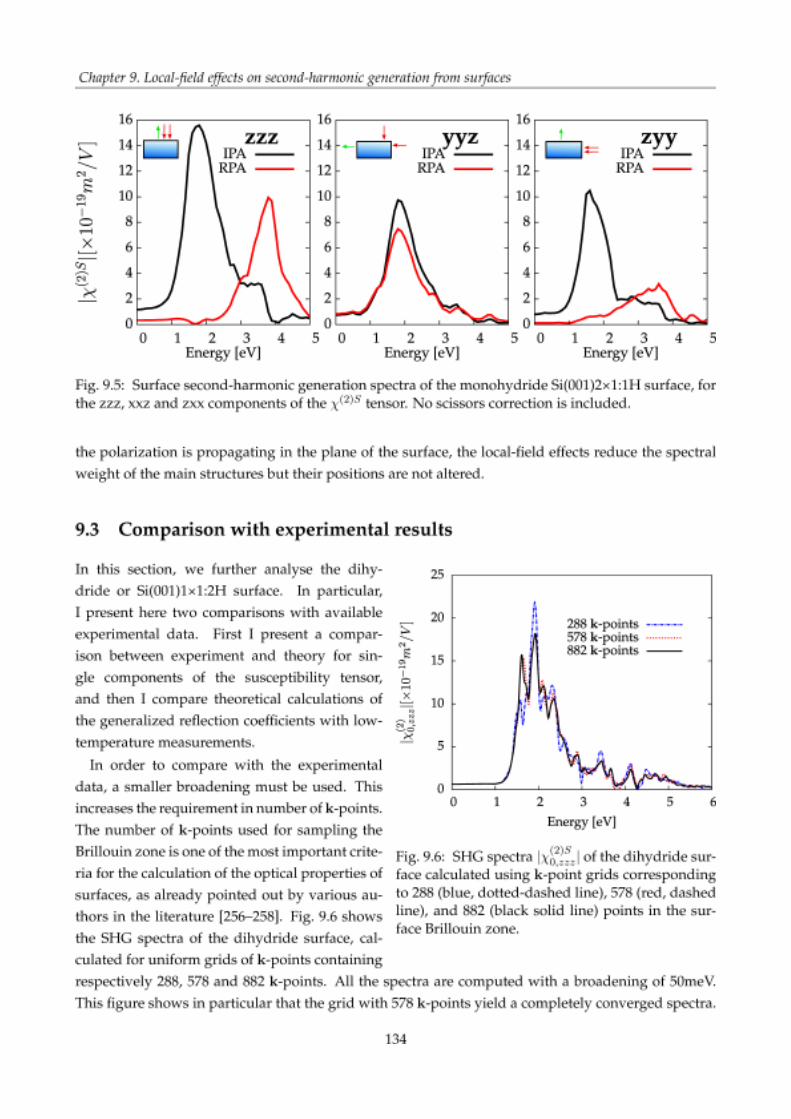
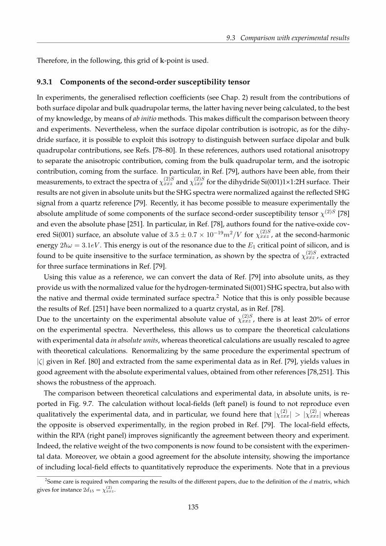
9.3 Comparison with experimental results
Therefore, in the following, this grid of k-point is used.
9.3.1 Components of the second-order susceptibility tensor
In experiments, the generalised reflection coefficients (see Chap. 2) result from the contributions ofboth surface dipolar and bulk quadrupolar terms, the latter having never being calculated, to the bestof my knowledge, by means of ab initio methods. This makes difficult the comparison between theoryand experiments. Nevertheless, when the surface dipolar contribution is isotropic, as for the dihy-dride surface, it is possible to exploit this isotropy to distinguish between surface dipolar and bulkquadrupolar contributions, see Refs. [78–80]. In these references, authors used rotational anisotropyto separate the anisotropic contribution, coming from the bulk quadrupolar term, and the isotropiccontribution, coming from the surface. In particular, in Ref. [79], authors have been able, from theirmeasurements, to extract the spectra of χ(2)S
xxz and χ(2)Szxx for the dihydride Si(001)1×1:2H surface. Their
results are not given in absolute units but the SHG spectra were normalized against the reflected SHGsignal from a quartz reference [79]. Recently, it has become possible to measure experimentally theabsolute amplitude of some components of the surface second-order susceptibility tensor χ(2)S [78]and even the absolute phase [251]. In particular, in Ref. [78], authors found for the native-oxide cov-ered Si(001) surface, an absolute value of 3.5 ± 0.7 × 10⁻¹⁹m2/V for χ(2)S
xxz , at the second-harmonicenergy 2hω = 3.1eV . This energy is out of the resonance due to the E1 critical point of silicon, and isfound to be quite insensitive to the surface termination, as shown by the spectra of χ(2)S
xxz , extractedfor three surface terminations in Ref. [79].
Using this value as a reference, we can convert the data of Ref. [79] into absolute units, as theyprovide us with the normalized value for the hydrogen-terminated Si(001) SHG spectra, but also withthe native and thermal oxide terminated surface spectra.2 Notice that this is only possible becausethe results of Ref. [251] have been normalized to a quartz crystal, as in Ref. [78].Due to the uncertainty on the experimental absolute value of χ(2)S
xxz , there is at least 20% of erroron the experimental spectra. Nevertheless, this allows us to compare the theoretical calculationswith experimental data in absolute units, whereas theoretical calculations are usually rescaled to agreewith theoretical calculations. Renormalizing by the same procedure the experimental spectrum of|ζ| given in Ref. [80] and extracted from the same experimental data as in Ref. [79], yields values ingood agreement with the absolute experimental values, obtained from other references [78,251]. Thisshows the robustness of the approach.
The comparison between theoretical calculations and experimental data, in absolute units, is re-ported in Fig. 9.7. The calculation without local-fields (left panel) is found to not reproduce evenqualitatively the experimental data, and in particular, we found here that |χ(2)
zxx| > |χ(2)xxz| whereas
the opposite is observed experimentally, in the region probed in Ref. [79]. The local-field effects,within the RPA (right panel) improves significantly the agreement between theory and experiment.Indeed, the relative weight of the two components is now found to be consistent with the experimen-tal data. Moreover, we obtain a good agreement for the absolute intensity, showing the importanceof including local-field effects to quantitatively reproduce the experiments. Note that in a previous
2Some care is required when comparing the results of the different papers, due to the definition of the d matrix, whichgives for instance 2d15 = χ
(2)xxz .
135

Chapter 9. Local-field effects on second-harmonic generation from surfaces
Fig. 9.7: Comparison between the theoretical calculation of |χ(2)Sxxz | and |χ(2)S
zxx | without local-field ef-fects (left panel), with local-field effects (middle panel), and the experimental data, from Ref. [79](right panel). Here we used ∆ω = 0.125eV , η = 0.25eV and scissors correction of ∆ = 0.6eV .
study of surface second-harmonic generation, performed at the level of independent-particles [228],the calculated intensities were found to be respectively a factor-of-5 and a factor-of-10 larger than theexperimental ones for Rpp and Rps.
The calculated peak positions are not in good agreement with the experimental one. It has beenobserved that the temperature has a strong influence on the peak position of the clean and the mono-hydride surfaces; and that lowering the temperature induces a blue-shift of the E1 resonance [33,253].The experimental data presented here have been obtained from room temperature measurements.Comparing the SHG spectra of Refs. [33, 58, 259], I found that decreasing the temperature from 300Kto 80K induces a blue-shift of about 0.1eV (in two-photon energy scale). Clearly, this does not explainentirely the difference in the peak positions found here of about 0.3 eV (in the two-photon energyscale). Even if we do not have a clear explanation for this discrepancy, we want to stress that state-of-the-art linear calculations, including the excitonic effects thanks to the Bethe-Salpeter equation, andwith a GW correction, instead of a scissors operator, also suffer from a 0.2 eV blue-shift as comparedto the experimental spectra for the dihydride surface [181]. This is consistent with the 0.3 eV of dif-ference we obtained, in the two-photon energy scale. Possible explanations for this difference in thepeak positions can be found in Ref. [181], and are therefore not repeated here. Finally, the calculationare performed here for 24 atomic layers. Calculations for thicker slabs are expected to improve theagreement with the experiment.
136
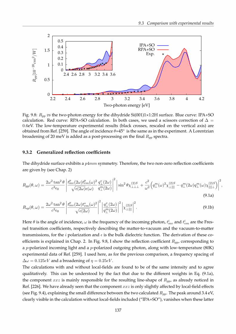
9.3 Comparison with experimental results
Fig. 9.8: Rpp vs the two-photon energy for the dihydride Si(001)1×1:2H surface. Blue curve: IPA+SOcalculation. Red curve: RPA+SO calculation. In both cases, we used a scissors correction of ∆ =0.6eV. The low-temperature experimental results (black crosses, rescaled on the vertical axis) areobtained from Ref. [259]. The angle of incidence θ=45° is the same as in the experiment. A Lorentzianbroadening of 20 meV is added as a post-processing on the final Rpp spectra.
9.3.2 Generalized reflection coefficients
The dihydride surface exhibits a p4mm symmetry. Therefore, the two non-zero reflection coefficientsare given by (see Chap. 2)
Rpp(θ, ω) =2ω2 tan2 θ
c3ǫ0
∣
∣
∣
∣
∣
tpmv(2ω)tpvm(ω)2
√
ǫ(2ω)ǫ(ω)
qv⊥(2ω)
qm⊥ (2ω)
∣
∣
∣
∣
∣
2 ∣∣
∣
∣
sin2 θχ(2)S⊥⊥⊥ +
c2
ω2
(
qm⊥ (ω)2χ(2)S⊥‖‖ − qm⊥ (2ω)qm⊥ (ω)χ
(2)S‖‖⊥
)
∣
∣
∣
∣
2
,
(9.1a)
Rsp(θ, ω) =2ω2 tan2 θ
c3ǫ0
∣
∣
∣
∣
∣
tpmv(2ω)tsvm(ω)2√
ǫ(2ω)
∣
∣
∣
∣
∣
2 ∣∣
∣
∣
qv⊥(2ω)
qm⊥ (2ω)
∣
∣
∣
∣
2 ∣∣
∣
∣
χ(2)S⊥‖‖
∣
∣
∣
∣
2
. (9.1b)
Here θ is the angle of incidence, ω is the frequency of the incoming photon, timv and tivm are the Fres-nel transition coefficients, respectively describing the matter-to-vacuum and the vacuum-to-mattertransmissions, for the i polarization and ǫ is the bulk dielectric function. The derivation of these co-efficients is explained in Chap. 2. In Fig. 9.8, I show the reflection coefficient Rpp, corresponding toa p-polarized incoming light and a p-polarized outgoing photon, along with low-temperature (80K)experimental data of Ref. [259]. I used here, as for the previous comparison, a frequency spacing of∆ω = 0.125eV and a broadening of η = 0.25eV .The calculations with and without local-fields are found to be of the same intensity and to agreequalitatively. This can be understood by the fact that due to the different weights in Eq. (9.1a),the component xxz is mainly responsible for the resulting line-shape of Rpp, as already noticed inRef. [226]. We have already seen that the component xxz is only slightly affected by local-field effects(see Fig. 9.4), explaining the small difference between the two calculatedRpp. The peak around 3.4 eV,clearly visible in the calculation without local-fields included (“IPA+SO”), vanishes when these latter
137

Chapter 9. Local-field effects on second-harmonic generation from surfaces
Fig. 9.9: Rpp spectra versus the incidence angle for the dihydride Si(001)1×1:2H surface. (a) Withoutlocal-field effects. (b) Local-field effects included. A Lorentzian broadening of 20 meV is added as apost-processing on the final Rpp spectra.
are included (“RPA+SO”). Again, we obtain that including local-field effects improve the compari-son with experiments. The results suggest that more interesting features can be observed at higherenergies, as shown by the big structure between 3.6 and 4.0 eV. From the results, it is also possibleto obtain the evolution of the reflection coefficient versus the angle of incidence. This is representedin Fig. 9.9. We observe that the Rpp reflection coefficient has the same angular dependence with andwithout local-field effects, except small structures between 3.2 and 3.4 eV which are not present oncelocal-field effects are included.
Fig. 9.10: The same as in Fig. 9.8, but forthe s-in/p-out reflection coefficient Rsp.
I would like to comment on the value of the angle of in-cidence chosen for studying the dihydride surface. The ex-perimental measurements of Ref. [259] (shown by the redline in Fig. 9.9) were performed at 45° of incidence. Otherstudies of the same surface were also performed with sim-ilar angles, for instance 35° [253] and 45° [227]. How-ever, as suggested by Fig. 9.9, the optimal value for per-forming measurements on the dihydride surface is around70°, as it would yield a more intense signal. An an-gular value around 70° is experimentally possible, e.g.,Ref. [260] where authors performed their measurementswith a value of 67.5° for their measurements on the cleanSi(001)2×1 surface. A more complex problem is to probethe higher-energy region, even if studies have been already performed in this region [63, 228].The absence of features in the reflection spectra from the dihydride surface is mainly due to the choiceof the incidence angle, and a more optimal value of the angle of incidence would potentially revealmore details in the second-harmonic reflection spectra of the dihydride surface.
In Fig. 9.8, I show the reflection coefficientRsp, corresponding to an s-polarized incoming light anda p-polarized outgoing photon. By opposition to the Rpp reflection coefficient, the local-fields quench
138

9.3 Comparison with experimental results
completely the spectra. Note that the spectra including local-field effects (“RPA+SO”) is rescaledby a factor of 50 to be compared to the spectra without local-field effects (“IPA+SO”). This is easilyunderstood, looking at Eq. (9.1b). Indeed, the Rsp coefficient depends only on the square of |χ(2)
zyy|,with the component zyy being strongly affected by the local-field effects in the region between 1 eVand 2 eV, for the fundamental frequency, see Fig. 9.7. Without the local-field effects, the intensity isover-estimated by more than a factor of 50, showing how crucial it is to account for the latter.
Summary
I have presented in this chapter the local-field effects on the surface second-harmonic generation,obtained for the first time from ab initio calculations. The local-fields have been taken into accountexactly, without assuming any model, using the theory developed in Chap. 7.Applied to the generation of second-harmonic from silicon surfaces, I have shown how impor-tant these local-fields are for describing the components of the second-order susceptibility tensor.Through the analysis of different components of three silicon surfaces, I have shown that two maineffects are possible. If the direction of the emitted polarization, i.e., the first component of the χ(2)S
tensor, is perpendicular to the plane of the surface (z-direction), the local-field effects are found tobe important and to redistribute the weight from 2ω transitions to 1ω transitions. If the outgoingpolarization is in the plane of the surface, the local-field effects are found to be less important and tonot affect the prominent peaks positions.I have also investigated in this chapter the effect of ad-atoms on the spectra of surface second-harmonic generation. In particular, I found a more important effect of the local-fields on the hy-drogenated surfaces. Interestingly, the major effect of local-fields, for the two hydrogenated surfaces,is to reduce the spectral weight drastically for some components of the χ(2)S tensor, in the regionwhere a quenching due to the hydrogen is found experimentally.Comparison with available experimental data have shown that these local-field effects allows us toobtain quantitative agreement between theory and experiments. We have compared theoretical cal-culations and experimental data, both in absolute units; showing for the first time an agreement forthe absolute intensity of surface second-harmonic generation calculated from ab initio methods. Also,the comparisons with low temperature reflectivity measurements have shown an improvement of thetheoretical description, when including local-field effects. As a conclusion, we found that local-fieldeffects are mandatory for a good description of surface second-harmonic generation and that thetheory presented in this chapter takes us a step closer to reality.
139


10. Excitonic effects on second-harmonicgeneration from silicon surfaces
The electron-hole interaction is known to be a key ingredient for obtaining reliable results when cal-culating optical properties of bulk materials [261], but also surfaces [262] and nanostructures [263].When these effects are neglected, it is generally found that the absorption spectra is underestimatedin the low-energy region and overestimated the higher energy region.The state-of-the art method for including the excitonic effects in the optical spectra, namely solv-ing the Bethe-Salpeter equation (BSE), is still numerically challenging for surfaces, due to the bignumber of atoms that has to be treated. An alternative way for including excitonic effects is thetime-dependent-density-functional theory (TDDFT), where these effects are obtained through theinclusion of the variations of the exchange-correlation (xc) potential. Various exchange-correlationkernels (fxc) have been proposed during the twenty past years, mainly for extended systems, andonly few of them have been tested on surfaces. Among these few kernels, we find the long-rangecontribution (LRC) kernel, or α-kernel [114], which includes the correct long-range decay of fxc inmomentum space as 1/q2. This simple kernel has been found to be sufficient to obtain the contin-uum exciton effects in optical spectra of bulk semiconductors, like GaAs and silicon. It has also beensuccessfully tested against the result of the BSE for the linear optical properties of the Si(111)2×1 sur-face [262]. Authors of Ref. [262] found the α-kernel to be applicable to surfaces of semiconductors,with the value of α determined for the bulk material. Moreover this kernel has also been applied tothe calculation of SHG spectra, thus improving the agreement with the experiment [41, 43].In this chapter, I show that it is possible to extend the TDDFT macroscopic formalism developed inChap. 7, in order to include the exchange-correlation kernel fxc in the formalism. In the first part, Ishow that the effects of the LRC kernel, which is chosen to be a scalar kernel, can be included in thespectra, as a post-processing on the bulk measurable quantities, namely the macroscopic dielectrictensor, ǫM , and macroscopic second-order susceptibility tensor, χ(2)
M .Then I extend this derivation to the case of surfaces. In particular, I present a formula allowing usto include the effects of the α-kernel on the surface second-harmonic generation spectra. Finally, thisformalism is applied to the SHG spectra of silicon surfaces, to get an insight into the excitonic effectson the surface second-harmonic generation.This chapter represents the first effort to include such excitonic effects on the nonlinear properties ofsurfaces.
141

Chapter 10. Excitonic effects on second-harmonic generation from silicon surfaces
10.1 The α-kernel as a post-processing
10.1.1 Bulk materials
Let us start by considering bulk materials. Even if this does not correspond to the scope of thischapter, the results presented in this section serves as a preliminary for the surface case.
Macroscopic dielectric tensor
We start by considering the case of the macroscopic dielectric tensor of a bulk materials. In theframework of the TDDFT, and assuming the long-wavelength limit, the longitudinal-longitudinal(LL) part of the macroscopic dielectric tensor is given, at any level of approximation, by
ǫLLM (q;ω) =1
1 + v0(q)[
χ(1)ρρ (q;ω)
]
G=G′=0
, (10.1)
where q is a vanishing momentum, ω the frequency of the light, G and G′ are reciprocal latticevectors, and χ(1)
ρρ is the density response function of the fully interacting electronic system.The latter quantity is obtained in reciprocal space by solving the Dyson-like equation
[
χ(1)ρρ (q;ω)
]
GG′ =[
χ(0)ρρ (q;ω)
]
GG′ +∑
G1G2
[
χ(0)ρρ (q;ω)
]
GG1
[
v(q) + fxc(q;ω)]
G1G2
[
χ(1)ρρ (q;ω)
]
G2G′ ,
(10.2)where χ(0)
ρρ is the density response function of the non-interacting system, v is the Coulomb inter-action and fxc is the exchange-correlation kernel. In order to be able to solve this equation, onehas to introduce an approximation for the unknown exchange-correlation kernel. In the random-phase approximation (RPA), the exchange-correlation kernel is neglected and only the Coulomb in-teraction, responsible for the local-field effects, is considered (see Chap. 3). We denote χ(1)RPA
ρρ thesolution of Eq. (10.2) in the RPA. When the long-range contribution kernel is included, we have[
fLRCxc (q;ω)
]
G1G2= α/q2δG10δG1G2
. It is straightforward to show that the solution of the Dyson
equation including the long-range contribution, χ(1)ρρ , is linked to the RPA response, χ(1)RPA
ρρ , by
[
χ(1)ρρ (q;ω)
]
GG′ =[
χ(1)RPAρρ (q;ω)
]
GG′ +[
χ(1)RPAρρ (q;ω)
]
G0
α
q2[
χ(1)ρρ (q;ω)
]
0G′ . (10.3)
From Eq. 10.3, we obtain that χ(1)00 (q;ω) =
χ(1)RPA00 (q;ω)
(
1−χ(1)RPA00 (q;ω) α
q2
) . Using this result, the macroscopic
dielectric response including the effect of the LRC kernel, ǫM , can then be linked to the macroscopicRPA dielectric response, ǫRPA
M . After simple algebra, one obtains that
ǫLLM (q;ω)− 1 =ǫLL,RPAM (q;ω)− 1
1 + α4π
(
ǫLL,RPAM (q;ω)− 1
). (10.4)
This simple formula can be used to obtain the effect of the LRC kernel on the linear spectra, at theextremely low cost of a post-processing of the dielectric response computed in the RPA. Notice thatthis analytical expression is close to the contact exciton model, as already discussed in Ref. [84].
142
10.1 The α-kernel as a post-processing
Second-order response function
The measurable quantity, playing the role of ǫLLM at second-order is the macroscopic second-orderresponse tensor χ(2)
M given by [41]
χ(2)M (q,q1,q2;ω, ω) =
−i2|q||q1||q2|
[
χ(2)ρρρ(q,q1,q2;ω, ω)
]
000ǫLLM (q; 2ω)ǫLLM (q1;ω)ǫ
LLM (q2;ω), (10.5)
where χ(2)ρρρ is the second-order susceptibility of the fully interacting electronic system; which can be
obtained by solving the second-order Dyson-like equation [41], see Eq. (3.37). We have defined hereq = q1 + q2.
We proceed following the same idea as for the linear case, and we link the RPA density responsefunction to the LRC density response function, i.e., containing the LRC exchange-correlation kernel.Following the derivation of App. F.2, we obtain the link between the solution of the Dyson equationincluding the long-range contribution, χ(2)
ρρρ, and the RPA response, χ(2)RPAρρρ , which reads in reciprocal
space as[
χ(2)ρρρ(q,q1,q2;ω, ω)
]
GG′G′′ =∑
G1G2
[
χ(2)RPAρρρ (q,q1,q2;ω, ω)
]
GG1G2
×[
δG1G′ +α
q21δG10
[
χ(1)ρρ (q1;ω)
]
G1G′
][
δG2G′′ +α
q22δG20
[
χ(1)ρρ (q2;ω)
]
G2G′′
]
+[
χ(1)RPAρρ (q; 2ω)
]
G0
α
q2[
χ(2)ρρρ(q,q1,q2;ω, ω)
]
0G′G′′ .
The solution of this equation for G = G′ = G′′ = 0 is
[
χ(2)ρρρ(q,q1,q2;ω, ω)
]
000=
[
χ(2)RPAρρρ (q,q1,q2;ω, ω)
]
000(
1− αq2
[
χ(1)RPAρρ (q; 2ω)
]
00
)
[
1+α
q21
[
χ(1)ρρ (q1;ω)
]
00
][
1+α
q22
[
χ(1)ρρ (q2;ω)
]
00
]
.
(10.6)Inserting the expressions of χ(2)
000 and χ(1)00 into Eq. 10.5, we obtain directly the link between the RPA
and the full macroscopic second-order susceptibilities
χ(2)M (q,q1,q2;ω, ω) =
−i2|q||q1||q2|
ǫLLM (q; 2ω)(
1− α4πv0(q)
[
χ(1)RPAρρ (q; 2ω)
]
00
)χ(2)RPA000 (q,q1,q2;ω, ω)
×[
ǫLLM (q1;ω)(
1− α4πv0(q1)
[
χ(1)RPAρρ (q1;ω)
]
00
)
][
ǫLLM (q2;ω)(
1− α4πv0(q2)
[
χ(1)RPAρρ (q2;ω)
]
00
)
]
,
where we used the fact that αq2
= α4πv0(q).
After some algebra and using the fact that
ǫLLM (q;ω) =
(
1 + α4π
)
ǫLL,RPAM (q;ω)− α
4π
1 + α4π
(
ǫLL,RPAM (q;ω)− 1
), (10.7)
143

Chapter 10. Excitonic effects on second-harmonic generation from silicon surfaces
we obtain the simple result
χ(2)M (q,q1,q2;ω, ω) = A(q; 2ω)χ
(2)RPAM (q,q1,q2;ω, ω)A(q1;ω)A(q2;ω), (10.8)
where A(q;ω) = 1
1+ α4π
(
ǫLL,RPAM (q;ω)−1
) .
Again we have linked the macroscopic quantity, including the long-range contribution χ(2)M , to the
RPA macroscopic second-order response χ(2)RPAM . This result allows us to include the excitonic effects
on the second-harmonic spectra of bulk materials, without increasing the numerical burden associ-ated with its calculation.
10.1.2 Surfaces
We have established that the effects of the α-kernel on the macroscopic optical responses of bulksystems can be included, at first- and second-order, as a post-processing of the macroscopic RPAoptical responses. In this section, I extend this result to the case of surfaces. The calculations aremore complex because of the presence, in the Dyson-like equations, of both the density responsefunctions and surface-averaged density response functions, see Chap. 7.
Surface dielectric function
The expression of the macroscopic surface dielectric function (see Chap. 7 for the definition and thederivation) is given by
ǫS,LLM (q;ω) = 1− limq→0
v0(q)1
Lz
∑
GzC(−Gz)
[
χ(1)ρρ (q;ω)
]
Gz0
1 + v0(q)[
χ(1)ρρ (q;ω)
]
00
, (10.9)
where Lz is the thickness of half of the super-cell used to model the surface.We introduce the quantity χ(1), defined by Eq. (7.16), which is related in the LRC approximation tothe density response function of the fully interacting system, χ(1)
ρρ , by
[
χ(1)(q;ω)]
G0=
[
χ(1)ρρ (q;ω)
]
G0
1 + (v0(q) +αq2)[
χ(1)ρρ (q;ω)
]
00
. (10.10)
Inserting this relation into the expression of the macroscopic dielectric tensor, and identifying themacroscopic dielectric tensor in the RPA approximation, given by Eq. (7.18), we obtain directly that
ǫS,LLM (q;ω)− 1 =(
ǫS,LL,RPAM (q;ω)− 1
)1 + (v0(q) +αq2)[
χ(1)ρρ (q;ω)
]
00
1 + v0(q)[
χ(1)ρρ (q;ω)
]
00
.
Simple algebra give that
1 + (v0(q) +αq2)[
χ(1)ρρ (q;ω)
]
00
1 + v0(q)[
χ(1)ρρ (q;ω)
]
00
= 1 +α
4π
v0(q)[
χ(1)ρρ (q;ω)
]
00
1 + v0(q)[
χ(1)ρρ (q;ω)
]
00
=1
1 + α4π
(
ǫLL,RPAM (q;ω)− 1
).
144

10.1 The α-kernel as a post-processing
Finally, we obtain that the macroscopic surface dielectric function is given by
ǫS,LLM (q;ω)− 1 =ǫS,LL,RPAM (q;ω)− 1
1 + α4π
(
ǫLL,RPAM (q;ω)− 1
), (10.11)
showing that the result of Eq. (10.4) is also valid for the surface macroscopic dielectric tensor.
Surface second-order susceptibility
Now that we have established the preliminary results, we can focus on the primary interest of thischapter, which is the analytical inclusion of the effect of the LRC-kernel in the macroscopic surfacesecond-order susceptibility.We start from the expression of the macroscopic surface second-order susceptibility, valid for anyapproximation of the exchange-correlation kernel, proved in Chap. 7
χ(2)SM (q,q1,q2;ω, ω) =
−i2|q||q1||q2|
ǫM (q1;ω)ǫM (q2;ω)
×[
(
ǫSM (q; 2ω)− 1)
[
χ(2)ρρρ(q,q1,q2;ω, ω)
]
000+ χ(2)S
ρρρ (q,q1,q2;ω, ω)
]
, (10.12)
where χ(2)Sρρρ (q,q1,q2;ω, ω) is given by
χ(2)Sρρρ (q,q1,q2;ω, ω) =
1
Lz
∑
Gz
C(Gz)[
χ(2)ρρρ(q,q1,q2;ω, ω)
]
Gz00. (10.13)
For conciseness, we omit here the LL superscript of the dielectric functions.Using Eq. (10.6) and Eq. (10.11), we obtain that
χ(2)SM (q,q1,q2;ω, ω) =
−i2|q||q1||q2|
A(q1;ω)ǫRPAM (q1;ω)A(q2;ω)ǫ
RPAM (q2;ω)
×[
A(q; 2ω)(
ǫS,RPAM (q; 2ω)− 1
)
[
χ(2),RPAρρρ (q,q1,q2;ω, ω)
]
000(
1− α4πv0(q)
[
χ(1)RPAρρ (q; 2ω)
]
00
) + χ(2)S,RPAρρρ (q,q1,q2;ω, ω)
+χS(q,q, ω)α
q2χ(2),RPAρρρ (q,q1,q2;ω, ω)
]
000
(
1 + v0(q)[
χ(1)RPAρρ (q; 2ω)
]
00
)
(
1− α4πv0(q)
[
χ(1)RPAρρ (q; 2ω)
]
00
)
]
. (10.14)
In order to simplify this expression, we first prove the following set of relations
1(
1− α4πv0(q)
[
χ(1)RPAρρ (q; 2ω)
]
00
)
= 1 +α
q2[
χ(1)ρρ (q; 2ω)
]
00, (10.15a)
(
1 + v0(q)[
χ(1)RPAρρ (q; 2ω)
]
00
)
(
1− α4πv0(q)
[
χ(1)RPAρρ (q; 2ω)
]
00
) = 1 + (v0(q) +α
q2)[
χ(1)ρρ (q; 2ω)
]
00,
= A(q; 2ω)(
1 + v0(q)[
χ(1)ρρ (q; 2ω)
]
00
)
, (10.15b)
145

Chapter 10. Excitonic effects on second-harmonic generation from silicon surfaces
A(q;ω)+A(q;ω)α
4π
(
ǫRPAM (q; 2ω)− 1
)
= 1, (10.15c)
χS(q,q, ω)α
q2= − α
4π
(
ǫS,RPAM (q; 2ω)− 1
)
. (10.15d)
Inserting all the ingredients above into the expression of the macroscopic surface second-order sus-ceptibility, we obtain, after some algebra,
χ(2)SM (q,q1,q2;ω, ω) =
−i2|q||q1||q2|
A(q; 2ω)A(q1;ω)ǫRPAM (q1;ω)A(q2;ω)ǫ
RPAM (q2;ω)
×[
(
ǫS,RPAM (q; 2ω)− 1
)
(
[
χ(2),RPAρρρ (q,q1,q2;ω, ω)
]
000− α
4π
[
χ(2),RPAρρρ (q,q1,q2;ω, ω)
]
000
)
+χ(2)S,RPAρρρ (q,q1,q2;ω, ω) +
α
4π
(
ǫRPAM (q; 2ω)− 1
)
χ(2)S,RPAρρρ (q,q1,q2;ω, ω)
]
.
(10.16)
We directly notice that if we replace the surface quantities by the bulk one, we recover the bulkexpression Eq. (10.8), thus showing the consistency of the approach.To make this more obvious, we identify Eq. (10.8) in Eq. (10.16), and we obtain
χ(2)SM (q,q1,q2;ω, ω) = A(q; 2ω)χ
(2)S,RPAM (q,q1,q2;ω, ω)A(q1;ω)A(q2;ω)
− i
2|q||q1||q2|α
4πA(q; 2ω)A(q1;ω)ǫ
LL,RPAM (q1;ω)A(q2;ω)ǫ
LL,RPAM (q2;ω)
×[
(
ǫLL,RPAM (q; 2ω)− 1
)
χ(2)S,RPAρρρ (q,q1,q2;ω, ω)−
(
ǫS,LL,RPAM (q; 2ω)− 1
)
[
χ(2),RPAρρρ (q,q1,q2;ω, ω)
]
000
]
.
(10.17)The second term in this expression appears as a correction to the bulk formula, in the case of surfaces.The formalism developed in Chap. 7 is valid only for symmetric slab. We now assume that the fullslab has the inversion symmetry, which is always possible to have with symmetric slab of centro-symmetric materials. This is the case for all the symmetric slab considered in this thesis. This impliesthat the term
[
χ(2),RPAρρρ (q,q1,q2;ω, ω)
]
000is zero. In this special case, we can simplify Eq. (10.17) to
obtain that
χ(2)SM (q,q1,q2;ω, ω) =
−iχ(2)S,RPAρρρ (q,q1,q2;ω, ω)
2|q||q1||q2|ǫRPAM (q1;ω)ǫ
RPAM (q2;ω)A(q1;ω)A(q2;ω)
= χ(2)S,RPAM (q,q1,q2;ω, ω)A(q1;ω)A(q2;ω)
(10.18)
This result is the main result of this chapter. It allows us to include the effect of the α-kernel on thesurface second-harmonic generation, as a post-processing on top of the RPA results. We do not haveto calculate nor to diagonalize the exciton Hamiltonian and the cost of the calculation is the cost ofthe RPA calculation. It is worthwhile to note that the last expression is not the same as the bulkformula. Indeed, we found that the “screening” term A(q; 2ω) is not present in Eq. (10.18), due to thesymmetries of the slab, used for performing the calculation.
146

10.2 Excitonic effects on the surface second-harmonic generation
Fig. 10.1: Surface second-harmonic generation spectra of the dihydride Si(001)1×1:2H surface, forthe zzz (left panel), the xxz (middle panel), and the zxx (right panel) components of the χ(2)S tensor.Black lines: IPA calculations. Red lines: RPA calculations. Blue lines: excitonic calculations using theα-kernel. A scissors operator (SO) correction of ∆ = 0.6 eV is included in all the calculations.
10.2 Excitonic effects on the surface second-harmonic generation
10.2.1 Effects on components of the susceptibility tensor
Here we discuss the effects of the long-range contribution kernel fxc on the surface second-order sus-ceptibility spectra. The value of α used is -0.2, as it has been found to well reproduce the BSE spectrafor the bulk silicon and the Si(111)2×1 surface [262].In Fig. 10.1, we show the excitonic effects on the surface second-harmonic spectra from the dihydridesurface, also including the local-field effects (blue lines), compared to the independent-particle spec-tra (black lines) and the spectra including only the effect of the local fields (red lines). As a generalresult, we find that the main effect of the α-kernel is to increase the magnitude of |χ(2)S
M | in the low en-ergy region. Notice that a similar effect has already been observed for bulk semiconductors [41,264].We also find that the excitonic effects almost do not change the position of the prominent peaks, byopposition to the local-field effects. Only a small red-shift of 0.1 eV is observed for the zzz and thezxx components.1 The main effect of the α-kernel is to enhance the peak corresponding to the E1
critical point of bulk silicon, at 3.4 eV. Also the peak corresponding to the E2 critical point, at 4.3 eV,is enhanced for the component zzz. The corresponding peak at 2.15 eV is also enhanced for the com-ponent xxz, thus compensating almost completely the effects of the local fields on this peak. TheseE1 and E2 related peaks are located at the same energy as the bulk silicon critical points [265], as weused the same scissors correction as for bulk silicon.The results of Fig. (10.1) show that the IPA and the RPA are not enough for describing the second-harmonic generation from surfaces, and that excitonic effects must be included for obtaining in the
1We checked (not shown) that this peak is a real shift, using the same approach of including or not the scissors operator,as explained in Chap. 9.
147

Chapter 10. Excitonic effects on second-harmonic generation from silicon surfaces
Fig. 10.2: The same as Fig. 10.1 for the clean Si(001)2×1 surface.
correct description of the surface second-harmonic generation.We find that the same conclusions hold for the clean surface of silicon, as shown in Fig. 10.2. In par-ticular, the effect on the E1 related peak of the inclusion of the exciton more than double its intensityfor the zzz component. For the yyz components, the two main structures, corresponding to the E1
and E2 critical points for 2ω transitions are enhanced, as well as the peak due to the surface-states,around 0.5 eV.
10.2.2 Effects on the reflection coefficients
Fig. 10.3: Rpp vs the two-photon energyfor the dihydride Si(001)1×1:2H surface.Curves are explained in the text.
It is interesting to investigate the excitonic effects on thegeneralized reflection coefficients. As a test case, I chosethe Rpp coefficient of the dihydride surface. This coeffi-cient has already been presented in Chap. 9, see Fig. 9.8.In Fig. 10.3, I reproduce the same data, adding the re-flection coefficient calculated with the excitonic effects in-cluded (blue curve), as explained above. In all the calcula-tions, I used a scissors correction of ∆ = 0.6eV . The low-temperature experimental results (black crosses, rescaledon the vertical axis) are obtained from Ref. [259]. The an-gle of incidence θ=45° is the same as in the experiment.A Lorentzian broadening of 20 meV is added as a post-processing on the final Rpp spectra.We directly see that in the region probed by the experi-ment, there is almost no excitonic effect visible, whereasaround 4.0 eV, we can see a change in the intensity, con-sistent with the behaviour obtain in Fig. 10.1 for the xxz component. The same conclusion hold forthe Rsp coefficient, which is also not affected by the excitonic effects, in the region considered here.
148
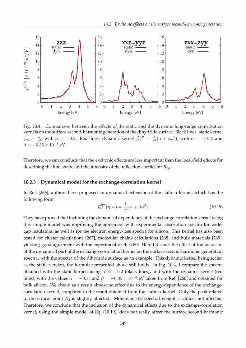
10.2 Excitonic effects on the surface second-harmonic generation
Fig. 10.4: Comparison between the effects of the static and the dynamic long-range contributionkernels on the surface second-harmonic generation of the dihydride surface. Black lines: static kernelfxc = α
q2, with α = −0.2. Red lines: dynamic kernel fdyn
xc = 1q2(α + βω2), with α = −0.13 and
β = −6.35× 10⁻³ eV.
Therefore, we can conclude that the excitonic effects are less important than the local-field effects fordescribing the line-shape and the intensity of the reflection coefficient Rpp.
10.2.3 Dynamical model for the exchange-correlation kernel
In Ref. [266], authors have proposed an dynamical extension of the static α-kernel, which has thefollowing form
fdynxc (q;ω) =
1
q2(α+ βω2). (10.19)
They have proved that including the dynamical dependency of the exchange-correlation kernel usingthis simple model was improving the agreement with experimental absorption spectra for wide-gap insulators, as well as for the electron energy-loss spectra for silicon. This kernel has also beentested for cluster calculations [267], molecular chains calculations [268] and bulk materials [269],yielding good agreement with the experiment or the BSE. Here I discuss the effect of the inclusionof the dynamical part of the exchange-correlation kernel on the surface second-harmonic generationspectra, with the spectra of the dihydride surface as an example. This dynamic kernel being scalar,as the static version, the formulae presented above still holds. In Fig. 10.4, I compare the spectraobtained with the static kernel, using α = −0.2 (black lines), and with the dynamic kernel (redlines), with the values α = −0.13 and β = −6.35 × 10⁻³ eV taken from Ref. [266] and obtained forbulk silicon. We obtain as a result almost no effect due to the energy-dependence of the exchange-correlation kernel, compared to the result obtained from the static α-kernel. Only the peak relatedto the critical point E2 is slightly affected. Moreover, the spectral weight is almost not affected.Therefore, we conclude that the inclusion of the dynamical effects due to the exchange-correlationkernel, using the simple model of Eq. (10.19), does not really affect the surface second-harmonic
149

Chapter 10. Excitonic effects on second-harmonic generation from silicon surfaces
spectra in energy region we are interested in, and that dynamical effects are negligible. Note that asimilar result for the absorption spectra of bulk GaAs was found in Ref. [270].
Conclusion
In this chapter, we have analysed the excitonic effects on the surface second-harmonic generation.The excitonic effects have been investigated using the α-kernel. I have proved in particular, that theeffects due to this static and scalar kernel can be including by a simple post-processing of the spectraincluding the local-field effects and the scissors correction, calculated within the RPA.Then we have analysed the excitonic effects on the surface second-harmonic generation spectra fromtwo silicon surfaces. We found that the excitonic effects increase the spectra weight of |χ(2)S
M |, and inparticular that they enhance the peak corresponding to the E1 critical point of bulk silicon. The peakpositions are almost not affected. The excitonic effects on the generalized reflection coefficient of thedihydride surface have also been investigated, showing only a small effect in the region probed bythe experiments whereas an effect is observed at higher energy, around the energy of the E2 criticalpoint of bulk silicon. We finally investigated the effects due to the dynamical extension of the α-kernel, showing almost no effect of the dynamical version against the static α-kernel.
150

Concluding Remarks
This thesis has been focusing on the ab initio description of the second-harmonic generation fromsurfaces, and more generally, I have tried to improve the theoretical description and understandingof the optical properties of crystalline surfaces.The second part of this thesis dealt with the microscopic description of the SHG from surfaces. Thetheory behind the calculation of the microscopic optical response of a single surface has been justi-fied, proved and tested with tight-binding calculations. The spatial construction of the SHG spectrahas been performed, showing that signal was mainly originating from the first layers and that thecontribution of deeper atomic layers was decaying, as expected from a surface signal. In Chap. 6,I have presented how to improve this microscopic description by taking into account the effect ofnonlocal operators, thus opening the way to more versatile and precise description of the second-harmonic generation from surfaces.However, a microscopic description of optical properties is not enough, due to microscopic fluctua-tions of the electric field and of the density. These fluctuations, called local-fields, and their effects onthe second-order optical properties of surfaces have been treated theoretically in Part. III. A macro-scopic theory has been presented, allowing us to take into account the local-field effects on the linearand second-order optical properties of a single surface. The analyticity of the macroscopic quantitycomputed has been proved. Most of the effort has been devoted to the clarification between themacroscopic optical response of a super-cell, which is the numerical tool for doing the calculation,and the surface, which is the physical system that we would like to treat. In particular, the super-cellapproach, due to the intrinsic periodicity induced by the approach, has been shown to fail in calcu-lating the out-of-plane optical response of a slab of matter, when including the effects of the localfields. The real space approach, which does not suffer from this problem, has been used to calculatethe correct optical response and, more importantly, to derive a new method, which merges the con-venience of the super-cell approach with the correctness of the treatment in real space.These developments have then been applied to silicon surfaces in Part. IV. The local-field effects onthe surface second-harmonic generation have been analysed on three silicon surfaces, in particularshedding some light on the important role of these local fields in the surface second-harmonic gen-eration.Finally, the excitonic effects have also been investigated in Chap. 10.It is clear that the developments of this thesis take us a step closer to the reality, as shown by thecomparisons with experiments presented in Chap. 9.Even if the theory seems now to be mature enough to give quantitative results, some points still need
151

Chapter 10. Excitonic effects on second-harmonic generation from silicon surfaces
to be addressed. Here are some of them. The excitonic effects have, so far, only been investigated bymeans of a simple scalar kernel. Even if these effects are found to be less important than local-fieldeffects, as shown by the results obtained with the long-range contribution kernel, their proper inclu-sion must not be forgotten for a quantitative description of surface second-harmonic generation.Then, even if very interesting results have been obtained for the hydrogen as an ad-atoms on sili-con surfaces, the effect of other ad-atoms like Ge or B has been experimentally well characterizedbut has to be understood and explained theoretically. Finally, two challenging elements are missing:the ab initio description of the bulk quadrupolar contribution, which should be sizeable comparedto the surface dipolar contribution and the ab initio description of the Electric Field Induced Second-Harmonic Generation (EFISH).
To summarize, the main original results of this thesis are:
1. Justification of the formalism of the microscopic description of the Second-Harmonic Genera-tion from surfaces, and improvement by including the effect of nonlocal operators.
2. Development of a macroscopic formalism for computing the optical response of a single sur-face, for linear and second-order optical properties.
3. Correct description of local-field effects on the out-of-plane optical response of surfaces.
4. First ab initio study of local-field effects on the second-harmonic generation spectra from cleanand hydrogenated silicon surfaces.
5. Investigation of the excitonic effects, for the first time, on the second-harmonic generation spec-tra from silicon surfaces.
Finally, I would like to comment this often quoted citation of the famous physicist Wolfgang Pauli"God made the bulk; surfaces were invented by the devil". For Wolfgang Pauli, the diabolical natureof surfaces was coming from the fact that surface atoms, instead of being surrounded by similaratoms as in bulk materials, were interacting with the external environment. This is maybe true, butthese interactions with the environment also lead to very interesting and exciting physics. I hopethat this thesis is a proof of how complex but also interesting the physics of surfaces is. Therefore, ifWolfgang Pauli was right, we should probably be grateful to the devil.
152

Part V
Appendices
153


A. Fourier transformsThe definition of the Fourier transform requires some care, because authors use different conventionsin the literature. In this appendix, I give the definitions of the Fourier transforms used in the thesis.
A.1 One-variable functions
Let us consider a function f ∈ L2, i.e., f is square integrable. The Fourier transforms in time and inspace for such a one-variable function f , as well as the reciprocal transformations are
f(ω) =
∫
dte−iωtf(t), f(t) =1
2π
∫
dωeiωtf(ω),
f(r) =1
(2π)3
∫
d3kf(k)eikr, f(k) =
∫
d3rf(r)e−ikr.
(A.1)
A practical application of these Fourier transforms is the definition of various Dirac’s delta func-tions
δ(t) =1
2π
∫
dωeiωt, δ(ω) =1
2π
∫
dte−iωt, (A.2a)
δ(k) =1
(2π)3
∫
d3re−ikr, δ(r) =1
(2π)3
∫
d3keikr. (A.2b)
A.2 Two-variable functions
Let us consider a two-variable functions, such as response functions.We consider a function χ, square integrable, and two functions f and g, such that f, g ∈ L2 and
f(r) =
∫
d3r′χ(r, r′)g(r′). (A.3)
The Fourier transform of this expression is
f(k) =
∫
d3k′χ(k,k′)g(k′). (A.4)
Using the definitions Eqs. (A.1), we obtain by identification
χ(r, r′) =1
(2π)3
∫
d3k
∫
d3k′eikrχ(k,k′)e−ik′r′ , (A.5a)
χ(k,k′) =1
(2π)3
∫
d3r
∫
d3r′e−ikrχ(r, r′)eik′r′ . (A.5b)
Similarly, in time, we obtain
χ(t, t′) =1
(2π)
∫
dω
∫
dω′eiωtχ(ω, ω′)e−iω′t′ , (A.6a)
155
Appendix A. Fourier transforms
χ(ω, ω′) =1
(2π)
∫
dt
∫
dt′e−iωtχ(t, t′)eiω′t′ . (A.6b)
A.3 Crystals and Fourier Transforms
When dealing with an infinite system, such as a crystal, we can replace this infinite system by a finitesystem of volume V, using some periodic boundary conditions. These conditions are called Born-
von-Karman periodic boundary conditions. The condition states that any functions of the crystal ffollows
f(r+Niai) = f(r), (A.7)
the ai are the primitive vectors of the lattice and Ni are integers, with i ∈ x, y, z.In a crystal of volume V, we can write 1
f(r) =1
V
∑
k
f(k)eikr, f(k) =
∫
Vd3rf(r)e−ikr. (A.8)
Equations A.2b become for example
δk,k′ =1
V
∫
Vd3re−i(k−k′)r, δ(r) =
1
V
∑
k
eikr. (A.9)
The equivalent of relation A.3 in a periodic crystal is
f(k1) =∑
k2
χ(k1,k2)g(k2) (A.10)
In crystals, any reciprocal vector k can be expressed as the sum of a vector q, belonging to the firstBZ of the crystal and a reciprocal lattice vector G.Using definitions A.8 and using the fact that the integral of a periodic function u
∫
V d3ru(r)e−ikr is
non zero only if k is a vector of reciprocal lattice G, we get
χG,G′(q) =1
V
∫
Vd3r
∫
Vd3r′e−i(q+G)rχ(r, r′)ei(q+G′)r′ ,
χ(r, r′) =1
V
∑
q,G,G′ei(q+G)rχG,G′(q)e−i(q+G′)r′ ,
(A.11)
where χG,G′(q) stands for χ(q + G,q + G′), q is a vector in the first Brillouin zone and G, G′ arevectors of the reciprocal lattice.
1Here the factor V is chosen to be on the inverse transform for not having volumes in Dyson-like equations and forhaving a Coulomb potential defined as 4π
q2and not 4π√
V q2or 4π
V q2
156

A.4 Fourier transform in the mixed-space
A.4 Fourier transform in the mixed-space
In Chap. 7, I defined the mixed-space. Here I give the different Fourier transforms, that link themixed-space with the real space and the reciprocal space. Let us consider the 2D Fourier transform,defined by
f(k||, z) =∫
dx
∫
dye−i(kxx+kyy)f(x, y, z). (A.12)
Using this definition, we obtain the following relations
f(k) =
∫
dze−ikzzf(k||, z), (A.13a)
f(k||, z) =1
2π
∫
dqzeikzzf(k). (A.13b)
We consider a two-variable function χ as the function describing the response f to a perturbation g.We have
f(k||, z) =∫
d2k′||
∫
dz′χ(k||, z,k′||, z
′)g(k′||, z
′). (A.14)
Hence,
χ(k,k′) =1
2π
∫
dz
∫
dz′e−ikzzχ(k||, z,k′||, z
′)eik′zz
′, (A.15a)
χ(k||,k′||, z1, z2) =
1
2π
∫
dkz
∫
dk′zeikzzχ(k,k′)e−ikz′z
′. (A.15b)
A.4.1 Periodic crystals
Considering that the system is periodic, one gets that
f(q+G) =
∫
dze−i(qz+Gz)zf(q|| +G||, z), (A.16a)
f(q|| +G||, z) =1
Lz
∑
qz ,Gz
ei(qz+Gz)zf(q+G), (A.16b)
where q is a vector in the first Brillouin zone, G is a reciprocal lattice vector, q = q|| + qz z andG = G||+Gz z. Here Lz is the size of the cell along the z-axis, which is then repeated to fill the space.We obtain for delta functions
δkzk′z=
1
Lz
∫
dze−i(kz−k′z)z, (A.17a)
δ(z) =1
Lz
∑
kz
eikzz. (A.17b)
One easily extend the definitions of the Fourier transforms to two-variable response functions
χG||1,G||2(q||, z1, z2) =1
Lz
BZ∑
qz
∑
Gz1,Gz2
ei(qz+Gz1)z1χG1,G2(q)e−i(qz+Gz2)z2 , (A.18a)
157
Appendix A. Fourier transforms
χG1,G2(q) =
1
Lz
∫
dz1dz2e−i(qz+Gz1)z1χG||1,G||2(q||, z1, z2)e
i(qz+Gz2)z2 , (A.18b)
χG||1,G||2(q||, z1, z2) =1
A
∫
d2r||1d2r||2e
−i(q||+G||1)r||1χ(r1, r2)ei(q||+G||2)r||2 , (A.18c)
χ(r1, r2) =1
A
BZ∑
q||
∑
G||1,G||2
ei(q||+G||1)r||1χG||1,G||2(q||, z1, z2)e−i(q||+G||2)r||2 , (A.18d)
where the A is the system area.For three-variable response functions, we obtain similarly,
χG1||,G2||,G3||(q||, z1, z2, z3) =1
A
∫
d2r1||d2r2||d
2r3||e−i(q||+G1||)r1||χ(r1, r2, r3)
×ei(q||+G2||)r2||ei(q||+G3||)r3|| (A.19a)
χ(r1, r2, r3) =1
A2
BZ∑
q||
∑
G1||G2||G3||
ei(q||+G1||)r1||χG1||,G2||,G3||(q||, z1, z2, z3)
×e−i(q||+G2||)r2||e−i(q||+G3||)r3|| (A.19b)
158

B. Maxwell’s equations
From a long view of the history of mankind — seen from, say, ten thousand years from now —there can be little doubt that the most significant event of the nineteenth century will be judged asMaxwell’s discovery of the laws of electrodynamics.
Richard Feynman, in The Feynman Lectures on Physics (1964) Volume II, 1-6
In this thesis, all the fields are treated in a purely classical way whereas the mater is describedby response functions computed quantum-mechanically. This corresponds to the framework of thesemi-classical dielectric theory. The Maxwell equations are given here in a medium, not in the vac-uum.
B.1 Microscopic Maxwell’s equations
If one considers the matter at atomistic level, microscopic Maxwell equations are
∇.E(r, t) = 4πη(r, t), ∇×B(r, t)− 1
c
∂E
∂t(r, t) =
4π
cj(r, t),
∇.B(r, t) = 0, ∇×E(r, t) +1
c
∂B
∂t(r, t) = 0,
(B.1)
where E and B are the microscopic electric and magnetic field quantities, η and j are the microscopiccharge and current densities, respectively 1.These two last quantities are connected by the continuity equation for charge and current
∇. j(r, t) +∂η
∂t(r, t) = 0. (B.2)
B.1.1 Separation of different contributions
When dealing with microscopic fields, one has to take care about which field is considered. Indeedthe fields that appear in equations (B.1) are total fields, not external fields.We denote by E the total field that can be separated into an external field Eext and an induced field Eind.By linearity, Maxwell equations hold for total fields or external fields and induced fields separately.The same separation is applied to charge density and current density.This leads to the definition of the electric polarization P and the magnetization M such that
ηind(r, t) = −∇P(r, t), jind(r, t) =∂P
∂t(r, t) +∇×M(r, t). (B.3)
1There is no D and H fields because all of the charges are included in η and j. [37].
159

Appendix B. Maxwell’s equations
B.2 Macroscopic Maxwell’s equations
The question of averaging must be treated carefully. According to [37], only spatial averaging isnecessary. Macroscopic quantities can be understand as quantities that vary slowly with respect tothe characteristic size of the considered medium. In the case of a crystal, the characteristic size isthe size of the unit cell. These macroscopic quantities result from the averaging of the microscopicone, over regions large compared to atomic separation but small compared to the wavelength ofthe perturbation [44]. The definition of the averaging procedure requires great cares. In Ref. [39],Mochán and Barrera defined a general averaging procedure, which then can be chosen to be anensemble-average, a spatial average or a wave-vector average. As an example, the spatial average ofa function F (r, t) with respect to a test function f(r) is defined by
〈F (r, t)〉 =∫
d3r′f(r′)F (r− r′, t), (B.4)
with f(r) a real function, non-zero in some neighbourhood of r = 0 and normalized over all space.The test function does not need to be defined but must only requires continuity and smoothnessproperties [39]. We can show easily that space and time derivatives, that enter in the equations,commute with the averaging operation.
∂
∂ri〈F (r, t)〉 =
∫
d3r′f(r′)∂F
∂ri(r− r′, t) =
⟨
∂F (r, t)
∂ri
⟩
, (B.5)
and∂
∂t〈F (r, t)〉 =
∫
d3r′f(r′)∂F
∂t(r− r′, t) =
⟨
∂F (r, t)
∂t
⟩
. (B.6)
The definition of the wave-vector truncation has been already given in Chap. 1 and is not reportedhere again.
Without restricting ourself to any specific averaging procedure, we define the macroscopic fieldsEM = 〈E〉 and BM = 〈B〉. From Eqs. (B.1), we obtain
∇.E = 4π〈η〉, ∇×B− 1
c
∂E
∂t=
4π
c〈j〉, (B.7a)
∇.B = 0, ∇×E+1
c
∂B
∂t= 0. (B.7b)
In order to obtain the macroscopic Maxwell equations, we must use the following results (that areproved in [37], under dipole approximation)
〈η〉 = ρ−∇P, 〈j〉 = J+∂P
∂t+ c∇×M. (B.8)
Here, ρ and J are the macroscopic averaged free charge and free current densities (see Eq. (B.3)).There is nevertheless a limit to that approach, when the external fields are not macroscopic, becauseit is not possible to define macroscopic quantities, e.g., in the case of X-ray spectroscopy where thewavelength is very short.
160

B.2 Macroscopic Maxwell’s equations
The macroscopic Maxwell equations reads in real space by [37]
∇.DM (r, t) = 4πρ(r, t), ∇×HM (r, t)− 1
c
∂DM
∂t(r, t) =
4π
cJ(r, t),
∇.BM (r, t) = 0, ∇×EM (r, t) +1
c
∂BM
∂t(r, t) = 0,
(B.9)
where DM and HM are respectively the macroscopic electric displacement and macroscopic magneticfield.This macroscopic current and charge densities are connected by the continuity equation for chargeand current
∇J(r, t) +∂ρ
∂t(r, t) = 0. (B.10)
For the reader more at home with SI-notation, the preceding equations are in SI notation:
∇.DM (r, t) = ρ(r, t), ∇×HM (r, t)− ∂D
∂t(r, t) = J(r, t),
∇.BM (r, t) = 0, ∇×EM (r, t) +∂BM
∂t(r, t) = 0.
(B.11)
B.2.1 Separation of charges
The main problem when working with P and M is that these quantities are not uniquely defined andone has to choose a convention to define them. In this thesis, we chose the separation of charges thatwrites
D(r, t) = Eext(r, t). (B.12)
As consequences, we get
4πP = −Eind,4π
cM = Bind. (B.13)
Using the definition of the microscopic dielectric function ǫ
D(r, t) =
∫
d3r′∫
dt↔ǫ (r, r′, t− t′)E(r′, t′), (B.14)
we get that
Eext(r, t) =
∫
d3r′∫
dt↔ǫ (r, r′, t− t′)E(r′, t′) or E(r, t) =
↔ǫ−1
(r, r′, t− t′)Eext(r′, t′). (B.15)
Here↔ǫ−1
is the inverse of the dielectric tensor↔ǫ . In this thesis, I assume that
↔ǫ is always invertible.
The constitutive relations connecting EM and BM to DM and HM are giving by equations (B.16):
DM (r, t) = EM (r, t) + 4πPM (r, t), HM (r, t) = BM (r, t)− 4πMM (r, t), (B.16)
where PM and MM are respectively the macroscopic polarization and magnetization.
161

Appendix B. Maxwell’s equations
B.3 Longitudinal and Transverse Fields
In reciprocal space, the Maxwell equations Eqs. (B.9) reads as
ik.D(k;ω) = 4πρ(k;ω), ik×H(k;ω)− iω
cD(k;ω) =
4π
cJ(k;ω),
ik.B(k;ω) = 0, ik×E(k;ω) +iω
cB(k;ω) = 0.
(B.17)
Due to the structure of these equations, it is natural to divide the fields into longitudinal and transverse
fields. For a field E, the longitudinal part EL and transverse part ET are defined in reciprocal spaceas2
EL(k;ω) =k
k
(
E(k;ω).k
k
)
, ET (k;ω) = E(k;ω)−EL(k;ω) = −k
k×(
k
k×E(k;ω)
)
. (B.18)
Therefore the Maxwell equations become
DL(k;ω) =4πρ(k;ω)
k2k, i
k
k×HT (k;ω)− iω
cDT (k;ω) =
4π
cJT (k;ω),
BL(k;ω) = 0, k×ET (k;ω) +ωk
cBT (k;ω) = 0.
(B.19)
And the continuity equation becomes JL(k;ω) + ωρ(k;ω) = 0.
2In 1858, Helmholtz proved that any vector field E can be decomposed into a longitudinal and a transverse part [271],E = EL +ET , where EL and ET are defined, in real space, by ∇×EL = 0, and ∇.ET = 0.This is known as the Helmholtz decomposition.
162

C. Second-harmonic reflection coefficientsfor some symmetries
In chapter 2, I have presented the expressions of the four reflection coefficients Rpp, Rps, Rsp and Rss
for the p4mm symmetry. Here I report the expressions of these reflection coefficients in the generalcase, meaning when no symmetry is assumed for reducing the number of components. I also givethe simplified expressions in the case of the m symmetry corresponding to a single domain of theclean Si(001)2×1 surface, the p2mm symmetry corresponding to a single domain of the monohydrideSi(001)2×1:H surface and the 3m symmetry corresponding to the Si(111)1×1:H surface.
C.1 Reflection coefficients in the general case
Here we give the expression of the four reflection coefficients assuming no symmetry. In the generalcase, the χ(2)S tensor has 18 independent components in the case of the second-harmonic generation,due to the intrinsic symmetry property of the crystal which gives χ(2)S
ijk = χ(2)Sikj .
Rpp(θ, φ, ω) =ω2
2c3ǫ0
1
cos2 θ
∣
∣
∣
∣
∣
tpmv(2ω)tpvm(ω)2
√
ǫ(2ω)ǫ(ω)
∣
∣
∣
∣
∣
2 ∣∣
∣
∣
qv⊥(2ω)
qm⊥ (2ω)
∣
∣
∣
∣
2
×∣
∣
∣
∣
sin3 θχ(2)Szzz +
2c
ωqm⊥ (ω) sin2 θ
[
cosφχ(2)Szzx + sinφχ(2)S
zzy
]
+c2
ω2sin θqm⊥ (ω)2
[
cos2 φχ(2)Szxx + 2 cosφ sinφχ(2)S
zxy + sin2 φχ(2)Szyy
]
− c
2ωsin2 θqm⊥ (2ω)
[
cosφχ(2)Sxzz + sinφχ(2)S
yzz
]
− c2
ω2sin θqm⊥ (ω)qm⊥ (2ω)
[
cos2 φχ(2)Sxxz + cosφ sinφ(χ(2)S
xyz + χ(2)Syxz ) + sin2 φχ(2)S
yyz
]
− c3
2ω3qm⊥ (ω)2qm⊥ (2ω) cosφ
[
cos2 φχ(2)Sxxx + sin(2φ)χ(2)S
xxy + sin2 φχ(2)Sxyy
]
− c3
2ω3qm⊥ (ω)2qm⊥ (2ω) sinφ
[
cos2 φχ(2)Syxx + sin(2φ)χ(2)S
yyx + sin2 φχ(2)Syyy
]
∣
∣
∣
∣
2
, (C.1a)
Rps(θ, φ, ω) =ω2
2c3ǫ0
1
cos2 θ
∣
∣
∣
∣
tsmv(2ω)tpvm(ω)2
ǫ(ω)
∣
∣
∣
∣
2 ∣∣
∣
∣
qv⊥(2ω)
qm⊥ (2ω)
∣
∣
∣
∣
2
×∣
∣
∣
∣
sin2 θ(
sinφχ(2)Sxzz − cosφχ(2)S
yzz
)
+2c
ωsin θqm⊥ (ω)
[
sin2 φχ(2)Sxyz + cosφ sinφ(χ(2)S
xxz − χ(2)Syyz )− cos2 φχ(2)S
yzx
]
+c2
ω2qm⊥ (ω)2 sinφ
[
sin2 φχ(2)Sxyy + sin(2φ)χ(2)S
xxy + cos2 φχ(2)Sxxx
]
− c2
ω2qm⊥ (ω)2 cosφ
[
sin2 φχ(2)Syyy + sin(2φ)χ(2)S
yyx + cos2 φχ(2)Syxx
]
∣
∣
∣
∣
2
, (C.1b)
163
Appendix C. Second-harmonic reflection coefficients for some symmetries
Rsp(θ, φ, ω) =ω2
2c3ǫ0
1
cos2 θ
∣
∣
∣
∣
∣
tpmv(2ω)tsvm(ω)2√
ǫ(2ω)
∣
∣
∣
∣
∣
2 ∣∣
∣
∣
qv⊥(2ω)
qm⊥ (2ω)
∣
∣
∣
∣
2
×∣
∣
∣
∣
sin θ[
cos2 φχ(2)Szyy − sin(2φ)χ(2)S
zyx + sin2 φχ(2)Szxx
]
− c
2ωqm⊥ (2ω) sinφ
[
cos2 φχ(2)Syyy − sin(2φ)χ(2)S
yyx + sin2 φχ(2)Syxx
]
− c
2ωqm⊥ (2ω) cosφ
[
cos2 φχ(2)Sxyy − sin(2φ)χ(2)S
xxy + sin2 φχ(2)Sxxx
]
∣
∣
∣
∣
2
, (C.1c)
Rss(θ, φ, ω) =ω2
2c3ǫ0
1
cos2 θ
∣
∣tsmv(2ω)tsvm(ω)2
∣
∣
2∣
∣
∣
∣
qv⊥(2ω)
qm⊥ (2ω)
∣
∣
∣
∣
2
×∣
∣
∣
∣
sin3 φχ(2)Sxxx − cosφ sin2 φ
(
χ(2)Syxx + 2χ(2)S
xxy
)
+ cos2 φ sinφ(
χ(2)Sxyy + 2χ(2)S
yyx
)
− cos3 φχ(2)Syyy
∣
∣
∣
∣
2
.
(C.1d)
C.2 Reflection coefficients for the m symmetry
We give here the expression for a m symmetry, where the only non-zero components of the χ(2)S ten-sor are χ(2)S
yyx , χ(2)Sxyy , χ
(2)Sxxx , χ
(2)Syyz , χ
(2)Sxxz , χ
(2)Szxx , χ
(2)Szyy , χ
(2)Sxzz , χ
(2)Szzx , χ
(2)Szzz (The mirror plan is perpendicular
to ey).This symmetry corresponds for instance to a single domain of the clean Si(001)2x1 surface.
Rpp(θ, φ, ω) =ω2
2c3ǫ0
1
cos2 θ
∣
∣
∣
∣
∣
tpmv(2ω)tpvm(ω)2
√
ǫ(2ω)ǫ(ω)
∣
∣
∣
∣
∣
2 ∣∣
∣
∣
qv⊥(2ω)
qm⊥ (2ω)
∣
∣
∣
∣
2
×∣
∣
∣
∣
sin3 θχ(2)Szzz +
2c
ωqm⊥ (ω) sin2 θ cosφχ(2)S
zzx +c2
ω2sin θqm⊥ (ω)2
[
cos2 φχ(2)Szxx + sin2 φχ(2)S
zyy
]
− c
2ωsin θqm⊥ (2ω)
(
sin θ cosφχ(2)Sxzz +
2c
ωqm⊥ (ω)
[
cos2 φχ(2)Sxxz + sin2 φχ(2)S
yyz
]
)
− c3
2ω3qm⊥ (ω)2qm⊥ (2ω) cosφ
[
cos2 φχ(2)Sxxx + sin2 φ(χ(2)S
xyy + 2χ(2)Syyx )
]
∣
∣
∣
∣
2
, (C.2a)
Rps(θ, φ, ω) =ω2
2c3ǫ0
sin2 φ
cos2 θ
∣
∣
∣
∣
tsmv(2ω)tpvm(ω)2
ǫ(ω)
∣
∣
∣
∣
2 ∣∣
∣
∣
qv⊥(2ω)
qm⊥ (2ω)
∣
∣
∣
∣
2 ∣∣
∣
∣
sin θ
(
χ(2)Sxzz +
2c
ωqm⊥ (ω) cosφ(χ(2)S
xxz − χ(2)Syyz )
)
+c2
ω2qm⊥ (ω)2
[
sin2 φχ(2)Sxyy + cos2 φ(χ(2)S
xxx − 2χ(2)Syyx )
]
∣
∣
∣
∣
2
, (C.2b)
Rsp(θ, φ, ω) =ω2
2c3ǫ0
1
cos2 θ
∣
∣
∣
∣
∣
tpmv(2ω)tsvm(ω)2√
ǫ(2ω)
∣
∣
∣
∣
∣
2 ∣∣
∣
∣
qv⊥(2ω)
qm⊥ (2ω)
∣
∣
∣
∣
2
×∣
∣
∣
∣
sin θ[
cos2 φχ(2)Szyy + sin2 φχ(2)S
zxx
]
− c
2ωqm⊥ (2ω) cosφ
[
cos2 φχ(2)Sxyy + sin2 φ(χ(2)S
xxx − 2χ(2)Syyx )
]
∣
∣
∣
∣
2
,
(C.2c)
Rss(θ, φ, ω) =ω2
2c3ǫ0
sin2 φ
cos2 θ
∣
∣tsmv(2ω)tsvm(ω)2
∣
∣
2∣
∣
∣
∣
qv⊥(2ω)
qm⊥ (2ω)
∣
∣
∣
∣
2 ∣∣
∣
∣
sin2 φχ(2)Sxxx + cos2 φ
(
χ(2)Sxyy + 2χ(2)S
yyx
)
∣
∣
∣
∣
2
.
(C.2d)
164

C.3 Reflection coefficients for the mm2 symmetry
C.3 Reflection coefficients for the mm2 symmetry
We give here the expression for a mm2 symmetry, where the only non-zero components of the χ(2)S
tensor are χ(2)Syyz , χ
(2)Sxxz , χ
(2)Szxx , χ
(2)Szyy , χ
(2)Szzz . This symmetry corresponds for instance to a single domain
of the monohydride Si(001)2x1:H surface.
Rpp(θ, φ, ω) =ω2
2c3ǫ0tan2 θ
∣
∣
∣
∣
∣
tpmv(2ω)tpvm(ω)2
√
ǫ(2ω)ǫ(ω)
∣
∣
∣
∣
∣
2 ∣∣
∣
∣
qv⊥(2ω)
qm⊥ (2ω)
∣
∣
∣
∣
2 ∣∣
∣
∣
sin2 θχ(2)Szzz
+c2
ω2qm⊥ (ω)2
[
cos2 φχ(2)Szxx + sin2 φχ(2)S
zyy
]
− c2
ω2qm⊥ (2ω)qm⊥ (ω)
[
cos2 φχ(2)Sxxz + sin2 φχ(2)S
yyz
]
∣
∣
∣
∣
2
,
(C.3a)
Rps(θ, φ, ω) =1
2cǫ0sin2(2φ) tan2 θ
∣
∣
∣
∣
tsmv(2ω)tpvm(ω)2
ǫ(ω)
∣
∣
∣
∣
2 ∣∣
∣
∣
qv⊥(2ω)qm⊥ (ω)
qm⊥ (2ω)
∣
∣
∣
∣
2 ∣∣
∣
∣
χ(2)Sxxz − χ(2)S
yyz
∣
∣
∣
∣
2
, (C.3b)
Rsp(θ, φ, ω) =ω2
2c3ǫ0tan2 θ
∣
∣
∣
∣
∣
tpmv(2ω)tsvm(ω)2√
ǫ(2ω)
∣
∣
∣
∣
∣
2 ∣∣
∣
∣
qv⊥(2ω)
qm⊥ (2ω)
∣
∣
∣
∣
2 ∣∣
∣
∣
cos2 φχ(2)Szyy + sin2 φχ(2)S
zxx
∣
∣
∣
∣
2
, (C.3c)
Rss(ω) = 0. (C.3d)
C.4 Reflection coefficients for the 3m symmetry
We give here the expression for a 3m symmetry, where the only non-zero components of the χ(2)S ten-sor are χ(2)S
zzz = χ⊥⊥⊥, χ(2)Sxxz = χ
(2)Syyz = χ
(2)S‖‖⊥ , χ
(2)Szxx = χ
(2)Szyy = χ
(2)S⊥‖‖ , χ
(2)Sxxx = −χ(2)S
xyy = −χ(2)Syyx = χ
(2)S‖‖‖
(The mirror plan is perpendicular to ey). This symmetry corresponds for instance to the Si(1111)1x1:Hsurface.
Rpp(θ, φ, ω) =ω2
2c3ǫ0
1
cos2 θ
∣
∣
∣
∣
∣
tpmv(2ω)tpvm(ω)2
√
ǫ(2ω)ǫ(ω)
∣
∣
∣
∣
∣
2 ∣∣
∣
∣
qv⊥(2ω)
qm⊥ (2ω)
∣
∣
∣
∣
2 ∣∣
∣
∣
sin3 θχ(2)S⊥⊥⊥
+c2
ω2sin θ
(
qm⊥ (ω)2χ(2)S⊥‖‖ − qm⊥ (ω)qm⊥ (2ω)χ
(2)S‖‖⊥
)
− c3
2ω3qm⊥ (ω)2qm⊥ (2ω) cos(3φ)χ
(2)S‖‖‖
∣
∣
∣
∣
2
,
(C.4a)
Rps(θ, φ, ω) =c
2ω2ǫ0
sin2(3φ)
cos2 θ
∣
∣
∣
∣
tsmv(2ω)tpvm(ω)2
ǫ(ω)
∣
∣
∣
∣
2 ∣∣
∣
∣
qv⊥(2ω)qm⊥ (ω)2
qm⊥ (2ω)
∣
∣
∣
∣
2 ∣∣
∣
∣
χ(2)S‖‖‖
∣
∣
∣
∣
2
, (C.4b)
Rsp(θ, φ, ω) =ω2
2c3ǫ0
1
cos2 θ
∣
∣
∣
∣
∣
tpmv(2ω)tsvm(ω)2√
ǫ(2ω)
∣
∣
∣
∣
∣
2 ∣∣
∣
∣
qv⊥(2ω)
qm⊥ (2ω)
∣
∣
∣
∣
2 ∣∣
∣
∣
sin θχ(2)S⊥‖‖ +
c
2ωqm⊥ (2ω) cos(3φ)χ
(2)S‖‖‖
∣
∣
∣
∣
2
,
(C.4c)
Rss(θ, φ, ω) =ω2
2c3ǫ0
sin2(3φ)
cos2 θ
∣
∣tsmv(2ω)tsvm(ω)2
∣
∣
2∣
∣
∣
∣
qv⊥(2ω)
qm⊥ (2ω)
∣
∣
∣
∣
2 ∣∣
∣
∣
χ(2)S‖‖‖
∣
∣
∣
∣
2
. (C.4d)
165
Appendix C. Second-harmonic reflection coefficients for some symmetries
C.5 Reflection coefficients for a cubic non-centrosymmetric bulk
From Eq. (2.29) we get directly the four usual reflection coefficients
Rpp(θ, φ, ω) =c
2ω2ǫ0tan2(θ) sin2(2φ)
∣
∣
∣
∣
∣
qv⊥(2ω)qm⊥ (ω)
qm⊥ (2ω)
tpmv(2ω)tpvm(ω)2
√
ǫ(2ω)ǫ(ω)
qm⊥ (ω)− qm⊥ (2ω)
qm⊥ (2ω) + 2qm⊥ (ω)
∣
∣
∣
∣
∣
2∣
∣
∣χ(2)xyz
∣
∣
∣
2,
(C.5a)
Rps(θ, φ, ω) =2
cǫ0tan2(θ) cos2(2φ)
∣
∣
∣
∣
qv⊥(2ω)
qm⊥ (2ω)
tsmv(2ω)tpvm(ω)2
ǫ(ω)
qm⊥ (ω)
[qm⊥ (2ω) + 2qm⊥ (ω)]
∣
∣
∣
∣
2∣
∣
∣χ(2)xyz
∣
∣
∣
2, (C.5b)
Rsp(θ, φ, ω) =ω2
2c3ǫ0tan2(θ) sin2(2φ)
∣
∣
∣
∣
∣
tpmv(2ω)tsvm(ω)2√
ǫ(2ω)
∣
∣
∣
∣
∣
2 ∣∣
∣
∣
qv⊥(2ω)
qm⊥ (2ω)[qm⊥ (2ω) + 2qm⊥ (ω)]
∣
∣
∣
∣
2 ∣∣
∣χ(2)xyz
∣
∣
∣
2, (C.5c)
Rss(ω) = 0. (C.5d)
Notice here that these reflection coefficients depend on both the incident and the azimuthal angles.
166

D. Matrix elements of V in a plane-wavesbasis
The inclusion of the nonlocal part of the pseudo-potential requires the evaluation of the matrix ele-ments of the modified velocity, as defined by Eq. (6.11). More precisely, we want to compute
〈n,k|q.V |n′,k〉 = 〈n,k|C(z)q. v + q. vC(z)2
|n′,k〉, (D.1)
with v = p + i[V nl, r]. Two contributions have to be computed separately: 〈n,k|C(z)q.p+q.pC(z)2 |n′,k〉
and 〈n,k|C(z)[Vnl,iq.r]+[V nl,iq.r]C(z)
2 |n′,k〉. Using the definition of the Bloch states Eq. (3.40), the firstterm is easily obtained
〈n,k|C(z)p+ pC(z)2
|n′,k〉 = −i2V
∑
G,G′c∗n,k(G)cn′,k(G
′)
×∫
d3r
[
e−i(k+G).rC(z)∇r(ei(k+G′).r)−∇r(e
−i(k+G).r)C(z)ei(k+G′).r
]
=1
2
∑
G,G′c∗n,k(G)cn′,k(G
′)[
2k+G+G′] δG||G′||F (Gz −G′z), (D.2)
where we have defined F (Gz) =1
2Lz
∫
dze−iGzzC(z), with 2Lz the height of the super-cell.In order to compute the term containing the commutator, we introduce the unity operator
〈n,k|C(z)[V nl, iq. r]|n′,k〉 =∑
G′′〈n,k|C(z)|k+G′′〉〈k+G′′|[V nl, iq. r]|n′,k〉,
where 〈r|k+G〉 = ei(k+G).r/√V , V being the volume of the super-cell.
Using the definition of Bloch states Eq. 3.40, we obtain that
〈n,k|C(z)|k+G′′〉 = 1√V
∑
G
c∗n,k(G)
∫
d3re−i(G−G′′).rC(z),
〈k+G′′|[V nl, iq. r]|n′,k〉 = 1√V
∑
G′cn′,k(G
′)〈k+G′′|[V nl, iq. r]|k+G′〉.
Putting everything together yields
〈n,k|C(z)[Vnl, iq. r] + [V nl, iq. r]C(z)
2|n′,k〉 = 1
2
∑
G,G′,G′′c∗n,k(G)cn′,k(G
′)
×[
〈k+G′′|[V nl, iq. r]|k+G′〉δG||G′′||F (Gz −G′′z) + 〈k+G|[V nl, iq. r]|k+G′′〉δG′||G′′||F (G
′′z −G′
z)
]
.
167

Appendix D. Matrix elements of V in a plane-waves basis
Using the notation K = k+G and in case of a Kleinman-Bylander separable-form pseudo-potential,we have [120] (see Ref. [121] for the notations)
〈K|V nl|K′〉 =∑
s
ei(K−K′).τsls∑
l=0
l∑
m=−l
ElFslm(K)F s∗
lm(K′), F slm(K) =
∫
d3reiK.rδV sl (r)Φ
pslm(r).
Using the relation i〈K|[V nl, r]|K′〉 = (∇K + ∇K′)〈K|V nl|K′〉, shown in Ref. [121], we obtain thenonlocal contribution to the velocity operator, as already implemented in DP [116] and 2light [117]codes
〈n,k|[V nl, ir]|n′,k〉 =∑
s
ls∑
l=0
l∑
m=−l
El
[
∑
G
c∗n,k(G)eiG.τs∇GFslm(K)
][
∑
G′cn′,k(G
′)e−iG′.τsF s∗lm(K′)
]
+
[
∑
G
c∗n,k(G)eiG.τsF slm(K)
][
∑
G′cn′,k(G
′)e−iG′.τs∇G′F s∗lm(K′)
]
.
(D.4)The nonlocal part of the modified velocity, i.e., containing the contribution of the commutator, isgiven by
〈n,k|C(z)[Vnl, iq. r] + [V nl, iq. r]C(z)
2|n′,k〉 = 1
2
∑
G,G′,G′′c∗n,k(G)cn′,k(G
′)
×[
(∇K′′ +∇K′)〈K′′|V nl|K′〉δG||G′′||F (Gz −G′′z) + (∇K +∇K′′)〈K|V nl|K′′〉δG′||G′′||F (G
′′z −G′
z)
]
.
After some algebra, we obtain the expression of the nonlocal contribution to the modified velocitymatrix elements
〈n,k|C(z)[Vnl, iq. r] + [V nl, iq. r]C(z)
2|n′,k〉 = 1
2
∑
s
ls∑
l=0
l∑
m=−l
El
(
∑
G′′eiG
′′.τs∇K′′F slm(K′′)
∑
G
c∗n,k(G)δG||G′′||F (Gz −G′′z)
)(
∑
G′cn′,k(G
′)e−iG′.τsF s∗lm(K′)
)
+
(
∑
G′′eiG
′′.τsF slm(K′′)
∑
G
c∗n,k(G)δG||G′′||F (Gz −G′′z)
)(
∑
G′cn′,k(G
′)e−iG′.τs∇K′F s∗lm(K′)
)
+
(
∑
G
c∗n,k(G)eiG.τs∇KFslm(K)
)(
∑
G′′e−iG′′.τsF s∗
lm(K′′)∑
G′cn′,k(G
′)δG′||G′′||F (G′′z −G′
z)
)
+
(
∑
G
c∗n,k(G)eiG.τsF slm(K)
)(
∑
G′′e−iG′′.τs∇K′′F s∗
lm(K′′)∑
G′cn′,k(G
′)δG′||G′′||F (G′′z −G′
z)
)
.
(D.5)In this last expression, a double sum over G vector is involved, making the calculation of the non-local part of the modified velocity operator more intricate and time consuming than for the bulkcounterpart.
168
E. Divergence-free expression of χSρρρ
Here I present a detailed derivation of the divergence-free expression Eqs. (6.14). The starting pointis the divergent expression Eq. (6.10). We first split Eq. (6.10) into three pieces
χS,Iρρρ(q, q1, q2, ω) =
−2
V ω3
∑
nn′n′′
BZ∑
k
〈n,k|qVΣ|n′,k〉〈n′,k|q1vΣ|n′′,k〉〈n′′,k|q2v
Σ|n,k〉(EΣ
nk − EΣn′k + 2ω + 2iη)
(fnk − fn′′k)
(EΣnk − EΣ
n′′k + ω + iη)+
(fn′k − fn′′k)
(EΣn′′k − EΣ
n′k + ω + iη)
+ (q1 ↔ q2), (E.1a)
χS,IIρρρ (q, q1, q2, ω) =
i
V ω3
∑
nn′
BZ∑
k
(fnk − fn′k)
2〈n,k|[
qR, q1vΣ]
|n′,k〉〈n′,k|q2vΣ|n,k〉
(EΣnk − EΣ
n′k + ω + iη)
+〈n,k|qVΣ|n′,k〉〈n′,k|
[
q1r, q2vΣ]
|n,k〉(EΣ
nk − EΣn′k + 2ω + 2iη)
+ (q1 ↔ q2), (E.1b)
χS,IIIρρρ (q, q1, q2, ω) =
1
V ω3
∑
n
BZ∑
k
fnk〈n,k|[
qr,[
q1r, q2VΣ]]
|n,k〉+ (q1 ↔ q2). (E.1c)
The last term vanishes from time-reversal symmetry.In order to be able to apply Sipe and coworkers transformation [185], we first show that the termn = n′ is zero in χS,I
ρρρ
χS,I,n=n′ρρρ (q, q1, q2, ω) =
−2
V ω3
∑
n=n′n′′
BZ∑
k
〈n,k|qVΣ|n,k〉〈n,k|q1vΣ|n′′,k〉〈n′′,k|q2v
Σ|n,k〉(EΣ
nk − EΣn′k + 2ω + 2iη)
(fnk − fn′′k)
(EΣnk − EΣ
n′′k + ω + iη)+
(fnk − fn′′k)
(EΣn′′k − EΣ
nk + ω + iη)+ (q1 ↔ q2)
.
(E.2)
Using k → −k, we obtain directly that the contribution n = n′ to χ(2)Iabc (ω) is zero. It is therefore
possible to follow Sipe and coworkers demonstration and to write that
1
ω3(EΣnk − EΣ
n′k + 2ω + 2iη)
(fnk − fn′′k)
(EΣnk − EΣ
n′′k + ω + iη)+
(fn′k − fn′′k)
(EΣn′′k − EΣ
n′k + ω + iη)
=Aω3
+Bω2
+Cω+F(ω).
As in Ref. [185], terms associated to A and C are zero thanks to time-reversal symmetry. We have toshown that the term associated with B is zero.
B(ω) = (fnk − fn′′k)
(EΣn′k − EΣ
nk)(EΣn′′k − EΣ
nk)
[
2
(EΣn′k − EΣ
nk)+
1
(EΣn′′k − EΣ
nk)
]
+(fn′k − fn′′k)
(EΣn′k − EΣ
nk)(EΣn′k − EΣ
n′′k)
[
2
(EΣn′k − EΣ
nk)+
1
(EΣn′k − EΣ
n′′k)
]
.
(E.3)
169

Appendix E. Divergence-free expression of χSρρρ
Using the following definitions, derived from k.p theory,1
∂vΣnn′
∂k= i
∑
n′′ /∈Dn,Dn′
[
rnn′′ vΣn′′n′ − vΣ
nn′′ rn′′n′]
+ i[vΣ, r]nn′ + i∆n′nrnn′ , (E.4a)
∂VΣnn′
∂k= i
∑
n′′ /∈Dn,Dn′
[
rnn′′VΣn′′n′ − V
Σnn′′ rn′′n′
]
+ i[VΣ, r]nn′ + irnn′∆n′n, (E.4b)
and the tensor↔T=
∑
i,j 6=i
fijVΣ
ij(k)vΣji(k)
EΣij(k)
2 , we obtain after some algebra that
∂↔T
∂k=∑
n,n′ 6=n
fnn′(k)
[
∂VΣnn′(k)
∂k
vΣn′n(k)
EΣnn′(k)2
+∂vΣ
n′n(k)
∂k
VΣnn′(k)
EΣnn′(k)2
− 2VΣ
nn′(k)vΣn′n(k)∆nn′
EΣnn′(k)3
]
= −′∑
n,n′,n′′V
Σnn′ vΣ
n′n′′ vΣn′′n
[
fn′n′′
EΣn′n(k)E
Σn′n′′(k)
(
2
EΣn′n(k)
+1
EΣn′n′′(k)
)
+fnn′′
EΣn′n(k)E
Σn′′n(k)
(
2
EΣn′n(k)
+1
EΣn′′n(k)
)]
−∑
n,n′ 6=n
3fnn′VΣnn′ vΣ
n′n∆nn′
EΣnn′(k)3
+∑
n,n′ 6=n
fnn′
[
vΣnn′∆n′nv
Σn′n
EΣnn′(k)3
+[VΣ, ir]nn′ vΣ
n′n
EΣnn′(k)2
− VΣnn′ [ir, vΣ]n′n
EΣnn′(k)2
]
.
The first three terms vanish thank to time-reversal symmetry. Invoking the same arguments as inRef. [185], the term associated to B is zero. Concerning the F term, we get
F(ω) =16
(EΣn′k − EΣ
nk)3(EΣ
nk − EΣn′k + 2ω + 2iη)
[
(fnk − fn′′k)
EΣn′n − 2EΣ
n′′n
+(fn′k − fn′′k)
EΣn′n − 2EΣ
n′n′′
]
+(fnk − fn′′k)
(EΣn′′k − EΣ
nk)3(2EΣ
n′′n − EΣn′n)(E
Σnk − EΣ
n′′k + ω + iη)
+(fn′k − fn′′k)
(EΣn′k − EΣ
n′′k)3(2EΣ
n′n′′ − EΣn′n)(E
Σn′′k − EΣ
n′k + ω + iη).
We thus obtain the two-band and three-band terms,
χS,I3bndρρρ (q, q1, q2, ω) =
2
V
∑
n 6=n′ 6=n′′
BZ∑
k
〈n,k|qVΣ|n′,k〉〈n′,k|q1vΣ|n′′,k〉〈n′′,k|q2v
Σ|n,k〉(2EΣ
n′′n − EΣn′n)
×
16(fnk − fn′k)
(EΣn′k − EΣ
nk)3(EΣ
nk − EΣn′k + 2ω + 2iη)
− (fnk − fn′′k)
(EΣn′′k − EΣ
nk)3(EΣ
nk − EΣn′′k + ω + iη)
+(fn′k − fn′′k)
(EΣn′k − EΣ
n′′k)3(EΣ
n′′k − EΣn′k + ω + iη)
+ (q1 ↔ q2), (E.6a)
χS,I2bndρρρ (q, q1, q2, ω) = − 2
V
∑
n 6=n′
BZ∑
k
(fnk − fn′k)〈n,k|qR|n′,k〉〈n′,k|q1r|n,k〉q2∆n′n
(EΣnk − EΣ
n′k)2
1It is interesting to note here that v and V follow the same sum-rule.
170

×
16
(EΣnk − EΣ
n′k + 2ω + 2iη)+
1
(EΣnk − EΣ
n′k + ω + iη)
+ (q1 ↔ q2). (E.6b)
We now use partial fraction development, to simplify χS,I3bndρρρ that we then split into χ3bnd
I and χ3bndII ,
such as χS,I3bndρρρ (q, q1, q2, ω) = χ3bnd
I (q, q1, q2, ω) + χ3bndII (q, q1, q2, ω), with
χ3bndI (q, q1, q2, ω) =
2i
V
∑
n 6=n′ 6=n′′
BZ∑
k
〈n,k|qR|n′,k〉〈n′,k|q1r|n′′,k〉〈n′′,k|q2r|n,k〉
− (2EΣn′′k − EΣ
n′k − EΣnk)
(EΣn′k − EΣ
nk)2
4(fnk − fn′k)
(EΣnk − EΣ
n′k + 2ω + 2iη)
− (2EΣnk − EΣ
n′k − EΣn′′k)
(EΣn′′k − EΣ
nk)2
(fnk − fn′′k)
(EΣnk − EΣ
n′′k + ω + iη)
+(2EΣ
n′k − EΣnk − EΣ
n′′k)
(EΣn′k − EΣ
n′′k)2
(fn′k − fn′′k)
(EΣn′′k − EΣ
n′k + ω + iη)
+ (q1 ↔ q2), (E.7a)
χ3bndII (q, q1, q2, ω) =
4i
V
∑
n 6=n′ 6=n′′
BZ∑
k
〈n,k|qR|n′,k〉〈n′,k|q1r|n′′,k〉〈n′′,k|q2r|n,k〉(2EΣ
n′′n − EΣn′n)
2(fnk − fn′k)
(EΣnk − EΣ
n′k + 2ω + 2iη)− (fnk − fn′′k)
(EΣnk − EΣ
n′′k + ω + iη)+
(fn′k − fn′′k)
(EΣn′′k − EΣ
n′k + ω + iη)
+ (q1 ↔ q2). (E.7b)
Let us now consider χS,IIρρρ . Using the relations
1
ω3(EΣnk − EΣ
n′k + ω + iη)=
1
ω3(EΣnk − EΣ
n′k)− 1
(EΣnk − EΣ
n′k)3(EΣ
nk − EΣn′k + ω + iη)
,
1
ω3(EΣnk − EΣ
n′k + 2ω + iη)=
1
ω3(EΣnk − EΣ
n′k)− 8
(EΣnk − EΣ
n′k)3(EΣ
nk − EΣn′k + 2ω + iη)
,
we obtain that
χS,IIρρρ (q, q1, q2, ω) =
2i
V
∑
nn′
BZ∑
k
(fnk − fn′k)〈n,k|[
qR, q1vΣ]
|n′,k〉〈n′,k|q1vΣ|n,k〉
[
1
ω3(EΣnk − EΣ
n′k)− 1
(EΣnk − EΣ
n′k)3(EΣ
nk − EΣn′k + ω + iη)
]
+ (q1 ↔ q2)
+i
V
∑
nn′
BZ∑
k
(fnk − fn′k)〈n,k|qVΣ|n′,k〉〈n′,k|[
q1r, q2vΣ]
|n,k〉[
1
ω3(EΣnk − EΣ
n′k)− 8
(EΣnk − EΣ
n′k)3(EΣ
nk − EΣn′k + 2ω + iη)
]
+ (q1 ↔ q2). (E.8)
171
Appendix E. Divergence-free expression of χSρρρ
The term containing 1ω3 vanishes using k → −k and n↔ n′. The remaining terms give
χS,IIρρρ (q, q1, q2, ω) =
−2
V
∑
nn′
BZ∑
k
(fnk − fn′k)〈n,k|
[
qR, q1vΣ]
|n′,k〉〈n′,k|q2r|n,k〉(EΣ
nk − EΣn′k)
2(EΣnk − EΣ
n′k + ω + iη)
− 8
V
∑
nn′
BZ∑
k
(fnk − fn′k)〈n,k|qR|n′,k〉〈n′,k|
[
q1r, q2vΣ]
|n,k〉(EΣ
nk − EΣn′k)
2(EΣnk − EΣ
n′k + 2ω + iη)+ (q1 ↔ q2).
(E.9)
Notice here that all energies are scissored energies. This is due to the presence of the term [r, vΣ],which is not possible to neglect. This term must be worked out in order to obtain the commutator[r,v] that we can neglect [117]. In order to do so, we use that (with n′ /∈ Dn)
∂vΣaij
∂kc= −i[rc, vΣa]ij − i
∑
l /∈Di,Dj
[
vΣail r
clj − rcilv
Σalj
]
− i∆aij r
cij , (E.10a)
∂vaij∂kc
= −i[rc, va]ij − i∑
l /∈Di,Dj
[
vailrclj − rcilv
alj
]
− i∆aij r
cij . (E.10b)
From Eq. (E.10a) we directly obtain
[rc, vΣa]nn′
(EΣnn′)
= i∂vΣa
nn′
∂kc1
(EΣnn′)
−∑
l /∈Dn,Dn′
[
vΣanl r
cln′ − rcnlv
Σaln′]
(EΣnn′)
− ∆ann′ rcnn′
(EΣnn′)
. (E.11)
Combining this expression with Eq. (E.10b) gives the link between the two commutators
[rc, vΣa]nn′
(EΣnn′)
=[rc, va]nn′
Enn′+
∑
l /∈Dn,Dn′
[
vanlrbln′ − rcnlv
aln′]
Enn′+
∆ann′rcnn′
Enn′+
∆cnn′rann′
Enn′
−∑
l /∈Dn,Dn′
[
vΣanl r
cln′ − rcnlv
Σaln′]
EΣnn′
− ∆ann′rcnn′
EΣnn′
− ∆cnn′rann′
EΣnn′
.
We obtain the same relations by replacing v with V and vΣ with VΣ.
[q1r, q2vΣ]n′n
(EΣn′n)
=[q1r, q2v]n′n
En′n+
∑
l /∈Dn,Dn′
[q2vn′lq1rln − q1rn′lq2vln]
En′n+
q1∆n′nq2rn′n
En′n+
q2∆n′nq1rn′n
En′n
−∑
l /∈Dn,Dn′
[
q2vΣn′lq1rln − q1rn′lq2v
Σln
]
EΣn′n
− q1∆n′nq2rn′n
EΣn′n
− q2∆n′nq1rn′n
EΣn′n
(E.13a)
[qR, q1vΣ]nn′
(EΣnn′)
=[qR, q1v]nn′
Enn′+
∑
l /∈Dn,Dn′
[q1vnlqRln′ − qRnlq1vln′ ]
Enn′+
q1∆nn′ qRnn′
Enn′+
q∆nn′ q1vnn′
Enn′
−∑
l /∈Dn,Dn′
[
q1vΣnlqRln′ − qRnlq1vln′
]
EΣnn′
− q1∆nn′ qRnn′
EΣnn′
− q∆nn′ q1rnn′
EΣnn′
. (E.13b)
172

Let us define E and F such that
E =−2
V
∑
nn′
BZ∑
k
(fnk − fn′k)〈n,k|
[
qR, q1vΣ]
|n′,k〉〈n′,k|q2r|n,k〉(EΣ
nk − EΣn′k)
2(EΣnk − EΣ
n′k + ω + iη)+ (q1 ↔ q2), (E.14a)
F =−8
V
∑
nn′
BZ∑
k
(fnk − fn′k)〈n,k|qR|n′,k〉〈n′,k|
[
q1r, q2vΣ]
|n,k〉(EΣ
nk − EΣn′k)
2(EΣnk − EΣ
n′k + 2ω + iη)+ (q1 ↔ q2). (E.14b)
We insert Eq. (E.13a).
E =−2
V
∑
nn′
BZ∑
k
(fnk − fn′k)〈n,k|[qR, q1v]|n′,k〉〈n′,k|q2r|n,k〉
(Enk − En′k)(EΣnk − EΣ
n′k)(EΣnk − EΣ
n′k + ω + iη)
− 2
V
∑
nn′
∑
l /∈Dn,Dn′
BZ∑
k
(fnk − fn′k)〈n,k|q1v|l,k〉〈l,k|qR|n′,k〉〈n′,k|q2r|n,k〉
(Enk − En′k)(EΣnk − EΣ
n′k)(EΣnk − EΣ
n′k + ω + iη)
+2
V
∑
nn′
∑
l /∈Dn,Dn′
BZ∑
k
(fnk − fn′k)〈n,k|qR|l,k〉〈l,k|q1v|n′,k〉〈n′,k|q2r|n,k〉
(Enk − En′k)(EΣnk − EΣ
n′k)(EΣnk − EΣ
n′k + ω + iη)
− 2
V
∑
nn′
BZ∑
k
(fnk − fn′k)〈n,k|q1r|n′,k〉〈n′,k|q2r|n,k〉q∆nn′
(Enk − En′k)(EΣnk − EΣ
n′k)(EΣnk − EΣ
n′k + ω + iη)
− 2
V
∑
nn′
BZ∑
k
(fnk − fn′k)〈n,k|qR|n′,k〉〈n′,k|q2r|n,k〉q1∆nn′
(Enk − En′k)(EΣnk − EΣ
n′k)(EΣnk − EΣ
n′k + ω + iη)
+2
V
∑
nn′
∑
l /∈Dn,Dn′
BZ∑
k
(fnk − fn′k)〈n,k|q1v
Σ|l,k〉〈l,k|qR|n′,k〉〈n′,k|q2r|n,k〉(EΣ
nk − EΣn′k)
2(EΣnk − EΣ
n′k + ω + iη)
− 2
V
∑
nn′
∑
l /∈Dn,Dn′
BZ∑
k
(fnk − fn′k)〈n,k|qR|l,k〉〈l,k|q1v
Σ|n′,k〉〈n′,kq2r|n,k〉(EΣ
nk − EΣn′k)
2(EΣnk − EΣ
n′k + ω + iη)
+2
V
∑
nn′
BZ∑
k
(fnk − fn′k)〈n,k|q1r|n′,k〉〈n′,k|q2r|n,k〉q∆nn′
(EΣnk − EΣ
n′k)2(EΣ
nk − EΣn′k + ω + iη)
+2
V
∑
nn′
BZ∑
k
(fnk − fn′k)〈n,k|qR|n′,k〉〈n′,k|q2r|n,k〉q1∆nn′
(EΣnk − EΣ
n′k)2(EΣ
nk − EΣn′k + ω + iη)
+(q1 ↔ q2). (E.15)
We note that due to the occupation numbers and the restriction of the sum over n′′, we have directlyn /∈ Dn′ ,Dn′′ , n′ /∈ Dn,Dn′′ and n′′ /∈ Dn,Dn′ . We can safely define matrix elements of the positionoperator for these sums. For conciseness, we introduce the notation
∑
nn′∑
n′′ /∈Dn,Dn′ →∑′
nn′n′′ ,first introduced by Bechstedt and co-workers in Ref. [189]. By symmetrisation and using the time-reversal symmetry, we obtain a simpler expression for E, and similarly, for F . We can redefine thetwo-band and three-band terms, to accounts for these new terms. Two contributions are obtained forthe two-band part, one local and denoted χ2bnd
l that is non-zero even is the potential is local, and a
173
Appendix E. Divergence-free expression of χSρρρ
nonlocal part χ2bndnl that vanishes in the case of a local potential.
χ2bndl (q, q1, q2, ω) =
−2
V
∑
n 6=n′
BZ∑
k
(fnk − fn′k)〈n,k|qR|n′,k〉〈n′,k|q1r|n,k〉q2∆n′n
(EΣnk − EΣ
n′k)2
((Enk − En′k) + (EΣnk − EΣ
n′k))
(Enk − En′k)
8
(EΣnk − EΣ
n′k + 2ω + 2iη)
+2(Enk − En′k)− (EΣ
nk − EΣn′k)
(Enk − En′k)
1
(EΣnk − EΣ
n′k + ω + iη)
+ (q1 ↔ q2)
(E.16a)
χ2bndnl (q, q1, q2, ω) =
−2
V
∑
nn′
BZ∑
k
(fnk − fn′k)
〈n,k|[qR, q1v]|n′,k〉〈n′,k|q2r|n,k〉(Enk − En′k)(E
Σnk − EΣ
n′k)(EΣnk − EΣ
n′k + ω + iη)
+4〈n,k|qR|n′,k〉〈n,k|[q1r, q2v]|n′,k〉
(Enk − En′k)(EΣnk − EΣ
n′k)(EΣnk − EΣ
n′k + 2ω + iη)
+ (q1 ↔ q2)
(E.16b)
The new three-band contributions are included in the definition of the χ3bndI , which now reads as
χ3bndI (q, q1, q2, ω) =
2i
V
∑
n 6=n′ 6=n′′
BZ∑
k
〈n,k|qR|n′,k〉〈n′,k|q1r|n′′,k〉〈n′′,k|q2r|n,k〉
(Enk + En′k − 2En′′k)
(Enk − En′k)
4(fnk − fn′k)
(EΣnk − EΣ
n′k)(EΣnk − EΣ
n′k + 2ω + iη)
− (2Enk − En′k − En′′k)
(En′′k − Enk)
(fnk − fn′′k)
(EΣn′′k − EΣ
nk)(EΣnk − EΣ
n′′k + ω + iη)
+(2En′k − Enk − En′′k)
(En′k − En′′k)
(fn′k − fn′′k)
(EΣn′k − EΣ
n′′k)(EΣn′′k − EΣ
n′k + ω + iη)
+ (q1 ↔ q2)
(E.17)
174
F. Macroscopic surface response functions
F.1 Charge conservation and cut-function
We consider the following replacement for the current and for the density ρ(1)(r, ω) → ρ(1)S(r, ω) =
C(z)ρ(1)(r, ω) and j(1)ind(r, ω) → j
(1)Sind (r, ω) = C(z)j(1)ind(r, ω) where C(z) is a cut function introduced here,
in order to select the response from a part of the system.Using vector calculus relations, one can write that
∇.(
jSind(r, ω))
= C(z)∇. (jind(r, ω)) + gradC(z).jind(r, ω). (F.1)
Inserting the continuity relation yields
∇.(
jSind(r, ω))
= ωρS(r, ω) + gradC(z). jind(r, ω). (F.2)
Here we choose to assume two approximations:Approximation 1: The system is invariant under the permutation z ↔ −z.Approximation 2: The function C(z) is a step function.
Using Approximation 2, one finds that
gradC(z). jind(r, ω) = ez. jind(r, ω)δ(z) = ez. jind(x, y, z = 0, ω). (F.3)
Due to Approximation 1, the plan z = 0 is a mirror plan of the system, imposing that jind is containedin the plan [x,y]. Thereby it results that
k. jSind(k, ω) = ωρSind(k, ω). (F.4)
Physically, this result shows that the charge is conserved in each half of the system separately.Replacing the current and the density by their expressions in terms of response functions [44], weobtain at first order and second-order
ω2χSρρ(k,k
′, ω) = k. χSjj(k,k
′, ω).k′ − 〈ρS〉δ(k− k′)k2, (F.5a)
ω3χSρρρ(k,k
′,k′′, ω) = k. χSjjj(k,k
′,k′′, ω) : k′.k′′. (F.5b)
Note that if the slab and the cut-function C(z) are equally shifted by z0, the same result is obtained.
F.2 Response function to the total macroscopic classical potential
at second-order
Let us define the total macroscopic classical potential, as
Vmac[ρ(1)](1) = Vext(1) +
∫
d32v0(1− 2)ρ(2). (F.6)
175
Appendix F. Macroscopic surface response functions
where v0 is the long-range part of the Coulomb potential.The density of the system reads as
ρ(1) = ρ(0)(1) + ρ(1)ind(1) + ρ
(2)ind(1), (F.7)
where ρ(0)(1) is the unperturbed density. Inserting this expression in Eq. (F.6), yields
Vmac[ρ(1)](1) = V(0)
mac(1) + V(1)
mac(1) + V(2)
mac(1), (F.8)
where
V(0)
mac(1) =
∫
d32v0(1− 2)ρ(0)(2) (F.9a)
V(1)
mac(1) = V(1)
ext (1) +
∫
d32v0(1− 2)ρ(1)ind(2) (F.9b)
V(2)
mac(1) = V(2)
ext (1) +
∫
d32v0(1− 2)ρ(2)ind(2) (F.9c)
I now define the response function to that total macroscopic classical potential, using the shortnotation of Chap. 3,
ρ(2)ind(1) =
∫
d2
∫
d3χρρρ(1,2,3)V(1)
mac(2)V(1)
mac(3) +
∫
d2χρρ(1,2)V(2)
mac(2). (F.10)
From this definition and the definition of the independent-particle response function and the fully-interaction response functions Eq. (3.36) (see Chap. 3), we obtain the two equations
χ(2)ρρρ(1,2,3) =
∫
d4d5χρρρ(1,4,5)[
δ(4− 2) +
∫
d6v0(4− 6)χ(1)ρρ (6,2)
]
×[
δ(5− 3) +
∫
d7v0(5− 7)χ(1)ρρ (7,3)
]
+
∫
d4
∫
d5χρρ(1,4)v0(4− 5)χ(2)ρρρ(5,2,3) (F.11a)
χρρρ(1,2,3) =
∫
d4
∫
d5χ(0)ρρρ(1,4,5)
[
δ(4− 2) +
∫
d6(
v(4− 6) + fxc(4,6))
χρρ(6,2)]
×[
δ(5− 3) +
∫
d7(
v(5− 7) + fxc(5,7))
χρρ(7,3)]
+
∫
d4
∫
d5χ(0)ρρ (1,4)
(
v(4− 5) + fxc(4,5))
χρρρ(5,2,3)
+
∫
d4
∫
d5
∫
d6χ(0)ρρ (1,4)gxc(4,5,6)χρρ(5,2)χρρ(6,3) (F.11b)
where v is the Coulomb potential without its long-range part. For obtaining the second relation, Iused that
V(1)
eff (1) = V(1)
mac(1) + V(1)
xc (1) +
∫
d32v(1− 2)ρ(1)ind(2) (F.12a)
V(2)
eff (1) = V(2)
mac(1) + V(2)
xc (1) +
∫
d32v(1− 2)ρ(2)ind(2) (F.12b)
176

G. Analytical expression of vG1,G2(q)
In this appendix, I report the derivation of the analytical expression of the modified Coulomb poten-tial. The modified Coulomb potential is defined by, (see Chap. 8)
vG1,G2
(q) =1
Lmatz
∫ 0
−Lz
dz1dz2e−i(qz+Gz1)z12π
e−|q||+G1||||z1−z2|
|q|| +G1|||ei(qz+Gz2)z2δG1||,G2|| . (G.1a)
Let us first define some notations, in order to ease the derivation
kz1 = qz + Gz1, kz2 = qz + Gz2, k|| = |q|| +G1|||, R = Lmatz .
Using these notations, we obtain that
vG1,G2
(q) =2π
Rk||
∫ 0
−Rdz1e
−ikz1z1
[
e−k||z1
∫ z1
−Rdz2e
(ikz2+k||)z2 + ek||z1∫ 0
z1
dz2e(ikz2−k||)z2
]
δG1||,G2||
(G.2a)
After some tedious algebra, we obtain the expression of the modified Coulomb potential
vG1,G2
(q) = 2πei(kz1−kz2)R
[
sinc([kz1 − kz2]R)
(k2z2 + k2||)+sinc([kz1 − kz2]R)
(k2z1 + k2||)
]
δG1||,G2||
+2πei(kz1−kz2)R
Rk||(k2z2 + k2||)(k2z1 + k2||)
[
− cos([kz1 − kz2]R)(k2|| − kz1kz2)
+ e−2k||R(
(k2|| − kz1kz2) cos([kz1 + kz2]R)− k||(kz1 + kz2) sin([kz1 + kz2]R))
]
δG1||,G2|| .
(G.3a)
It is possible to simplify further this expression, using that Gz1 = n12πLmatz
and Gz2 = n22πLmatz
, n1, n2 ∈ Z.We have
sinc([kz2 − kz1]R
2) = sinc([n2 − n1]π) = δkz1,kz2 ,
where sinc is defined as sinc(x) = sin(x)x . Similarly, we obtain that
cos([kz1 − kz2]R
2) = cos([Gz2 −Gz1]L
matz /2) = (−1)n1−n2 = (−1)
R(kz1−kz2)π .
Without any approximation, we obtain that
cos([kz1 + kz2]R
2) = cos(qzR)(−1)
R(kz1+kz2)π ,
sin([kz2 + kz1]R
2) = sin(qzR)(−1)
R(kz1+kz2)π .
177

Appendix G. Analytical expression of vG1,G2(q)
Putting everything together, we obtain that
vG1,G2
(q) =4π
|q+ G1|2δG1,G2
+4πδG1||,G2||
|q+ G1|2|q+ G2|2
[
− e−|q||+G1|||Lmatz sin(qzR)
Lmatz
(2qz + Gz1 + Gz2))
+e−|q||+G1|||Lmat
z cos(qzR)− 1
Lmatz |q|| +G1|||
(
|q|| +G1|||2 − (qz + Gz1)(qz + Gz2))
]
.
From that expression, we can easily show that, for R→ ∞,
vG1,G2
(q) =4π
|q+ G1|2δG1,G2
= vG1
(q)δG1,G2
. (G.5)
178

H. Mixed-space equations for SHG
Here I show that the mixed-space analytical results of Chap. 8 are also valid for the nonlinear second-order optical properties.
H.1 Second-order dyson equation in the mixed-space
The second-order Dyson equation in real-space and real-time is given by Eq. (3.37). In frequencyspace, the second-order Dyson equation is
χ(2)ρρρ(r, r
′, r′′, ω1, ω2) =
∫
dr4dr5χ(2)0 (r, r4, r5, ω1, ω2)
×[
δ(r4 − r′) +∫
dr6fuxc(r4, r6, ω1)χ(1)ρρ (r6r
′, ω1)]
×[
δ(r5 − r′′) +∫
dr7fuxc(r5, r7, ω2)χ(1)ρρ (r7, r
′′, ω2)]
+
∫
dr4dr5dr6χ(1)0 (r, r4, ω1 + ω2)gxc(r4, r5, r6, ω1, ω2)χ
(1)ρρ (r5, r
′, ω1)χ(1)ρρ (r6, r
′′, ω2)
+
∫
dr4dr5χ(1)0 (r, r4, ω1 + ω2)fuxc(r4, r5, ω1 + ω2)χ
(2)ρρρ(r5, r
′, r′′, ω1, ω2).
(H.1)
For conciseness, we omit the frequency dependence. Using the definition of Fourier transform (seeApp. A),we obtain that
χ(2)G||,G′||,G′′||
(q||, z, z′, z′′) =
∑
G4||G5||
∫
dz4dz5χ(2)0,G||G4||G5||
(q||, z, z4, z5)
×[
δ(z4 − z′)δG4||G′|| +∑
G6||
∫
dz6fuxc,G4||G6||(q||, z4, z6)χ(1)G6||G′||
(q||, z6, z′)]
×[
δ(z5 − z′′)δG5||G′′|| +∑
G7||
∫
dz7fuxc,G5||G7||(q||, z5, z7)χ(1)G7||G′′||
(q||, z7, z′′)]
+∑
G4||G5||G6||
∫
dz4dz5dz6χ(1)0,G||G4||
(q||, z, z4)gxc,G4||G5||G6||(r4, r5, r6)
×χ(1)G5||G′||
(q||, z5, z′)χ(1)
G6||G′′||(q||, z6, z
′′)
+∑
G4||G5||
∫
dz4dz5χ(1)0,G||G4||
(q||, z, z4)fuxc,G4||G5||(q||, z4, z5)χ(2)G5||,G′||G′′||
(q||, z5, z′, z′′).
(H.2)
179
Appendix H. Mixed-space equations for SHG
Assuming the random-phase approximation, we get
χ(2)G||,G′||,G′′||
(q||, z, z′, z′′) =
∑
G4||G5||
∫
dz4dz5χ(2)0,G||G4||G5||
(q||, z, z4, z5)
×[
δ(z4 − z′)δG4||G′|| +
∫
dz6vG4||(q||, z4, z6)χ(1)G4||G′||
(q||, z6, z′)]
×[
δ(z5 − z′′)δG5||G′′|| +
∫
dz7vG5||(q||, z5, z7)χ(1)G5||G′′||
(q||, z7, z′′)]
+∑
G4||
∫
dz4dz5χ(1)0,G||G4||
(q||, z, z4)vG4||(q||, z4, z5)χ(2)G4||,G′||G′′||
(q||, z5, z′, z′′).
(H.3)
H.2 Isolated system from periodic super-cell calculations
We now define the auxiliary response functions χ(1), χ(1)0 , χ(2), and χ(2)
0 , similarly to what is done inChap. 8. We obtain that
χ(2)G||,G′||,G′′||
(q||, z, z′, z′′) =
∑
G4||G5||
∫ 0
−Lmatz
dz4dz5χ(2)0,G||G4||G5||
(q||, z, z4, z5)
×[
δ(z4 − z′)δG4||G′|| +
∫ 0
−Lmatz
dz6vG4||(q||, z4, z6)χ(1)G4||G′||
(q||, z6, z′)]
×[
δ(z5 − z′′)δG5||G′′|| +
∫ 0
−Lmatz
dz7vG5||(q||, z5, z7)χ(1)G5||G′′||
(q||, z7, z′′)]
+∑
G4||
∫ 0
−Lmatz
dz4dz5χ(1)0,G||G4||
(q||, z, z4)vG4||(q||, z4, z5)χ(2)G4||,G′||G′′||
(q||, z5, z′, z′′).
(H.4)
Then, using the Fourier tranform Eqs. (8.12) and the fact that the three variables are equivalent, weget
χ(2)G,G′,G′′(q) =
∑
G4||G5
χ(1)0,GG4
(q)vG4G5(q)χ
(2)G5,G′G′′(q)
+∑
G4G5
χ(2)0,GG4G5
(q)[
δG4G′ +∑
G6
vG4G6(q)χ
(1)G6||G′||
(q)][
δG5G′′ +∑
G7
vG5G7(q)χ
(1)G7G′′(q)
]
,(H.5)
where v is defined by Eq. (8.14).Therefore, we checked that the Selected-G method can also be applied to second-order susceptibili-ties.
180
I. Optical properties of single surfaces
I presented, in Chap. 7 and Chap. 8, a theory for calculating the optical properties of a single surface,in reciprocal space and using a super-cell technique, now known as the Selected-G formalism. In theRandom-Phase Approximation (RPA), I have shown that the calculation of linear and second-orderoptical properties of surfaces are based on the knowledge of two quantities, χ(0)S
ρρ and χ(0)Sρρρ . In this
section, I briefly review the macroscopic theory of Chap. 7 and I give the analytical expressions ofχ(0)Sρρ and χ(0)S
ρρρ , referred here as the surface-averaged independent-particle response functions.For conciseness, I consider only the case of the nonlocal part of the pseudo-potential as a nonlocaloperator, and I assume no scissors correction. Similar formulae are obtained when including thescissors operator.
I.1 Linear optical properties of crystal surfaces
In Chap. 7, I have presented how to calculate, in the framework of TDDFT, the macroscopic dielectrictensor of a semi-infinite system, i.e., with a single surface; referred here as the surface dielectric tensor.Here we also use the Selected-G approach, see Chap. 8.In the RPA, and in the optical limit, the surface macroscopic dielectric tensor is given by (see Sec. 7.3)
ǫS,LLM (q;ω) = limq→0
1(
1− v(q)χ(0)Sρρ (q,q;ω)
)−1
G=G′=0
. (I.1)
Here q is a vanishing momentum and G, G′ are reciprocal lattice vectors. The frequency of theimpinging light is ω. Also v refers to the Coulomb interaction and the notation
[
χ(0)Sρρ (q;ω)
]
GG′
stands for χ(0)Sρρ (q + G,q + G′;ω). In our formalism, the matrix
[
χ(0)Sρρ (q;ω)
]
GG′ , is defined by thefollowing set of equations
[
χ(0)Sρρ (q;ω)
]
0G′ = χ(0)Sρρ (q,q+G′;ω),
[
χ(0)Sρρ (q;ω)
]
GG′ =[
χ(0)ρρ (q;ω)
]
GG′ , G 6= 0,(I.2)
where χ(0)ρρ is the independent-particle or Kohn-Sham response function.
The elements χ(0)Sρρ (q,q+G′;ω) are obtained from the independent-particle response function by
χ(0)Sρρ (q,q+G′;ω) =
1
Lz
∑
Gz
C(−Gz)[
χ(0)ρρ (q;ω)
]
GzG′ , (I.3)
with Lz , the thickness of half of the cell used to model the surface.Thereby, the construction of the matrix
[
χ(0)Sρρ (q;ω)
]
GG′ requires only the knowledge of the independent-particle or Kohn-Sham response function χ
(0)ρρ , which is given in reciprocal space by Eq. (8.3). By
181
Appendix I. Optical properties of single surfaces
inserting Eq. (8.3) into Eq. (I.3), we obtain
χ(0)Sρρ (q,q+G′;ω) =
2
NkVcell
∑
n,n′
BZ∑
k
fnn′ρSn,n′,k(q)〈n′,k+ q|ei(q+G′)r|n,k〉
(En,k − En′,k+q + ω + iη), (I.4)
with fnn′ = fn − fn′1 and
ρSn,n′,k(q) =1
Lz
∑
Gz
C(−Gz)〈n,k|e−i(q+Gz)r|n′,k+ q〉.
This quantity has to be evaluated in the optical limit, meaning for q → 0.The expression of ρSn,n′,k(q) is given by
ρSn,n′,k(q) =1
Lz
∑
Gz
C(−Gz)〈n,k|e−i(q+Gz)r|m,k+ q〉
=
∫
d3rφ∗n,k(r)1
Lz
∑
Gz
C(−Gz)e−iGzze−iqrφn,k+q(r)
=
∫
d3rφ∗n,k(r)C(z)e−iqrφn,k+q, (I.5)
where we recognized the Fourier transform of the cut-function C in the last equation.In the optical limit, q → 0 and therefore, from k.p perturbation theory, we get that
ρSn,n′,k(q → 0) = 〈n,k|C(z)|n′,k〉+∑
m/∈Dn′
〈n,k|C(z)|m,k〉〈m,k|qv|n′,k〉Em,k − En′,k
. (I.6)
The position operator r can be expressed into interband ri and interband re part defined by [272]
〈n,k|ri|m,k′〉 = δnmδ(k− k′) [ξnn+ i∇k]
〈n,k|re|m,k′〉 = (1− δnm)δ(k− k′)ξnm
where r = ri + re.Using this definition, allows us to remove the restriction of the sum, and we get
ρSn,n′,k(q → 0) = 〈n,k|C(z)− iqreC(z)|n′,k〉. (I.7)
The generalized derivative of any operator O is given by [272]
(Onm);k =∂Onm
∂k− iOnm(ξnn − ξmm)
In the paper, authors give the following relation [272]
〈n,k|[ri, O]|n′,k′〉 = iδ(k− k′) (Onm);k
1Occupation numbers are independent of the momentum, as we consider a cold semiconductor with filled bands.
182

I.1 Linear optical properties of crystal surfaces
From these relations, we obtain that for n′ /∈ Dn, we have
i〈n,k|[re, H]|n′,k′〉 = 〈n,k|v|n′,k′〉, (I.8)
because (Hnm);k = 0 for n′ /∈ Dn. From this result, we can compute the last term of Eq. I.7 for n′ /∈ Dn
i(En,k − En′,k)〈n,k|rC(z)|n′,k〉 = i
∫
d3rC(z)φ∗n,k(r)(En,kre − reEn′,k)φn′,k(r)
= i
∫
d3rφ∗n,k(r)C(z)(Hre − reH) + (Hre − reH)C(z)
2φn′,k(r)
= 〈n,k|C(z)v + vC(z)2
|n′,k〉. (I.9)
Here we recognize the expression of the modified velocity (see Eq. (6.11)).The final expression of ρSn,n′,k(q → 0) is
ρSn,n′,k(q → 0) = 〈n,k|C(z)|n′,k〉+ 〈n,k|q.V |n′,k〉En,k − En′,k
. (I.10)
For G′ = 0, and in the limit q → 0, χ(0)Sρρ reads as
χ(0)Sρρ (q,q;ω) =
2
NkVcell
∑
n,n′
BZ∑
k
fnn′
[
〈n,k|C(z)|n′,k〉〈n′,k|iq. r|n,k〉〈n′,k|q.v|n′,k〉(En,k − En′,k + ω + iη)2
+〈n,k|C(z)|n′,k〉〈n′,k|iq. r|n,k〉
(En,k − En′,k + ω + iη)+
〈n,k|q.V |n′,k〉〈n′,k|iq. r|n,k〉(En,k − En′,k)(En,k − En′,k + ω + iη)
]
+O(q3),
(I.11)
whereas for G′ 6= 0, we obtain
χ(0)Sρρ (q,q+G′;ω) =
2
NkVcell
∑
n,n′
BZ∑
k
fnn′
[
〈n,k|C(z)|n′,k〉〈n′,k|eiG′r′ |n,k〉〈n,k|q.v|n,k〉(En,k − En′,k + ω + iη)2
+〈n,k|q.V |n′,k〉〈n′,k|eiG′r′ |n,k〉
(En,k − En′,k)(En,k − En′,k + ω + iη)+
〈n,k|C(z)|n′,k〉〈n′,k|eiG′r′ |n,k〉(En,k − En′,k + ω + iη)
]
+O(q2).
(I.12)
The first term in Eq. (I.12) and in Eq. (I.11) vanishes, using k → −k and n ↔ n′ two times. The otherterms associated with C(z) do not vanish using the time-reversal symmetry. In order to prove thatthese terms are zero, we introduce the surface-averaged current-current response function,
↔χ(0)S
jj (q+G,q+G′;ω) = 〈ρS〉δGG′↔1 +
1
4NkVcell
∑
n,n′
BZ∑
k
fnn′
×〈n,k|[
e−i(q+G)rC(z)v + vC(z)e−i(q+G)r]
|n′,k+ q〉〈n′,k+ q|[
ei(q+G′)rv + vei(q+G′)r]
|n,k〉(En,k − En′,k+q + ω + iη)
− 1
NkVcell
∑
n
BZ∑
k
fn〈n,k|e−i(q+G)r[r, [r, Vnl]]|n,k〉δGG′ ,
(I.13)
183

Appendix I. Optical properties of single surfaces
where Vnl stands for C(z)Vnl+VnlC(z)2 , Vnl being the nonlocal part of the pseudo-potential (see Chap. 6).
In the limit q → 0, we obtain at the 0-th order in q, after some algebra, that
↔χ(0)S
jj (q,q;ω) = 〈ρS〉↔1 +
1
NkVcell
BZ∑
k
∑
n,n′fnn′
〈n,k|V |n′,k〉〈n′,k|v|n,k〉(En,k − En′,k + ω + iη)
− 1
NkVcell
BZ∑
k
∑
n
fn〈n,k|[r, [r, Vnl]]|n,k〉, (I.14a)
↔χ(0)S
jj (q,q+G′;ω) =1
2NkVcell
∑
n,n′
BZ∑
k
fnn′〈n,k|V |n′,k〉〈n′,k|
[
eiG′rv + veiG
′r]
|n,k〉(En,k − En′,k + ω + iη)
. (I.14b)
Using the conservation of charges (see App. F.1), we obtain the two equalities
ω2χ(0)Sρρ (q,q;ω) = q.
↔χ(0)S
jj (q,q;ω).q− 〈ρS〉q2, (I.15a)
ω2χ(0)Sρρ (q,q+G′;ω) = q.
↔χ(0)S
jj (q,q+G′;ω). (q+G′). (I.15b)
From the comparison between the left-hand side and the right-hand side of Eqs. (I.15), we concludethat, at lowest order in q, χ(0)S
ρρ (q,q;ω) is proportional to q2, and χ(0)Sρρ (q,q+G;ω) is proportional to
q.This proves that the terms associated with 〈n,k|C(z)|n′,k〉 in Eq. I.11 and Eq. I.12 vanish. Finally, weobtain, at the lowest order in q, that
χ(0)Sρρ (q,q;ω) =
2
NkVcell
∑
n,n′
BZ∑
k
fnn′〈n,k|q.V |n′,k〉〈n′,k|iq. r|n,k〉
(En,k − En′,k)(En,k − En′,k+q + ω + iη), (I.16a)
χ(0)Sρρ (q,q+G′;ω) =
2
NkVcell
∑
n,n′
BZ∑
k
fnn′〈n,k|q.V |n′,k〉〈n′,k|eiG′r′ |n,k〉
(En,k − Em,k)(En,k − En′,k + ω + iη). (I.16b)
These expressions are similar to the usual expressions for matrix elements of χ(0)ρρ ; except the re-
placement 〈n,k|q.v|n′,k〉 → 〈n,k|q.V |n′,k〉, which allows us to calculate the optical properties ofa single surface. Note that the expression for χ(0)S
ρρ (q,q;ω) was already presented in Chap. 5 for alocal-potential. It is worthwhile to note that the quantity χ(0)S
ρρ has been found to describe the sur-face optical response, starting from a macroscopic description of the optical response; but also froma microscopic description, see Chap. 5.
I.1.1 Second-order optical properties of crystal surfaces
In Chap. 7, I have proved that the nonlinear optical properties of surfaces are given, for the case ofsecond-harmonic generation, by
χ(2)S,LLLM (q,q1,q2;ω, ω) =
−i2|q||q1||q2|
ǫS,LLM (q; 2ω)χSρρρ(q,q1,q2;ω, ω)ǫ
LLM (q1;ω)ǫ
LLM (q2;ω), (I.17)
184

I.1 Linear optical properties of crystal surfaces
where χSρρρ is obtained by solving Eq. (7.47), whose solution is
χSρρρ(q,q1,q2;ω, ω) =
∑
G1G2G3
[
Id− χ(0)Sρρ (q; 2ω)v(q)
]−1
0G1
[
χ(0)Sρρρ (q,q1,q2;ω, ω)
]
G1G2G3
×[
Id+ v(q1)χρρ(q1;ω)]
G20
[
Id+ v(q2)χρρ(q2;ω)]
G30.
(I.18)
In the formalism developed in Chap. 7, the matrix[
χ(0)Sρρρ (q,q1,q2;ω, ω)
]
GG1G2is defined by the
following set of equations
[
χ(0)Sρρρ (q,q1,q2;ω, ω)
]
0G1G2= χ(0)S
ρρρ (q,q1 +G1,q2 +G2;ω, ω),[
χ(0)Sρρρ (q,q1,q2;ω, ω)
]
GG1G2=[
χ(0)ρρρ(q,q1,q2;ω, ω)
]
GG1G2, G 6= 0.
(I.19)
Here χ(0)Sρρρ (q,q1 + G1,q2 + G2;ω, ω) is defined by matrix elements of the independent-particle re-
sponse function, thanks to
χ(0)Sρρρ (q,q1 +G1,q2 +G2;ω, ω) =
1
Lz
∑
Gz
C(−Gz)[
χ(0)ρρρ(q,q1,q2;ω, ω)
]
GzG1G2, (I.20)
where the Kohn-Sham density-density-density response function χ(0)ρρρ is given by [41]
[
χ(0)ρρρ(q,q1,q2;ω, ω)
]
GG1G2=
2
NkVcell
∑
n,n′,n′′
BZ∑
k
〈n,k|e−i(q+G)r|n′,k+ q〉(Enk − En′,k+q + 2ω + 2iη)
[
(fn,k − fn′′,k+q2)〈n′,k+ q|ei(q1+G1)r′ |n′′,k+ q2〉〈n′′,k+ q2|ei(q2+G2)r′′ |n,k〉
(En,k − En′′,k+q2+ ω + iη)
+(fn,k − fn′′,k+q1)〈n′,k+ q|ei(q2+G2)r′ |n′′,k+ q1〉〈n′′,k+ q1|ei(q1+G1)r′′ |n,k〉
(En,k − En′′,k+q1+ ω + iη)
+(fn′,k+q − fn′′,k+q1)〈n′,k+ q|ei(q2+G2)r′ |n′′,k+ q1〉〈n′′,k+ q1|ei(q1+G1)r′′ |n,k〉
(En′′,k+q1− En′,k+q + ω + iη)
+(fn′,k+q − fn′′,k+q2)〈n′,k+ q|ei(q1+G1)r′ |n′′,k+ q2〉〈n′′,k+ q2|ei(q2+G2)r′′ |n,k〉
(En′′,k+q2− En′,k+q + ω + iη)
]
.
(I.21)
The derivation of the matrix elements of χ(0)Sρρρ is similar to the derivation at matrix elements of χ(0)S
ρρ .Note that the head of the matrix,
[
χ(0)Sρρρ
]
000, has already been given in Chap. 6, see Eq. (6.13) and
Eqs. (6.14). Therefore, only the expressions for[
χ(0)Sρρρ
]
0G′0,[
χ(0)Sρρρ
]
00G′′ and[
χ(0)Sρρρ
]
0G′G′′ remains tobe derived.As their derivations follow exactly the same idea, I do not report the corresponding derivations here.The resulting expressions are found to be similar to the expressions for bulk materials, with only thereplacement 〈n,k|q.v|n′,k〉 → 〈n,k|q.V |n′,k〉 for the matrix elements associated with q.Matrix elements associated with q1 and q2 are identical to those of the “usual” bulk formula.
185


List of publications related to this work• Tancogne-Dejean, Nicolas and Mendoza, Bernardo S. and Véniard, Valérie.
Effect of material properties on the accuracy of antiresonant approximation: Linear and second-order optical responses.Phys. Rev. B. 90, 035212 (2014).
• Anderson, Sean M. and Tancogne-Dejean, Nicolas and Mendoza, Bernardo S. and Véniard,Valérie.Theory of surface second-harmonic generation for semiconductors including effects of nonlocaloperators.Phys. Rev. B. 91, 075302 (2015).
• Tancogne-Dejean, Nicolas, Giorgetti Christine and Véniard, Valérie.Optical properties of surfaces with supercell calculations: local-field effects.Submitted.
• Tancogne-Dejean, Nicolas and Véniard, Valérie.Ab initio macroscopic linear and second-order optical properties of crystal surfaces: From theslab to the single surface.In preparation.
• Tancogne-Dejean, Nicolas and Véniard, Valérie.Local-field effects on second-harmonic generation from surfaces.In preparation.
• Tancogne-Dejean, Nicolas and Véniard, Valérie.Excitonic effects on second-harmonic generation from silicon surfaces.In preparation.
187


List of the different codes used during thiswork
• Abinit [115].Ground state calculation.Reciprocal-space and plane-wave basis-set.
• DP [116].TDDFT in linear response at first order.Reciprocal-space and plane-wave basis-set.
• 2light [117].TDDFT in linear response at second-order.Reciprocal-space and plane-wave basis-set.
• TB_Si.Ground-state and linear response at first and second-order, within the IPA.Reciprocal-space and tight-binding orbital basis (sp3, sp3s∗, and sp3d5s∗).
189


Bibliography[1] Weinberger, P. Philosophical Magazine Letters, 88, 897–907 (2008) .
[2] Franken, P. A., Hill, A. E., Peters, C. W., and Weinreich, G. Phys. Rev. Lett., 7, 118–119 (1961) .
[3] Bass, M., Franken, P. A., Ward, J. F., and Weinreich, G. Phys. Rev. Lett., 9, 446–448 (1962) .
[4] New, G. H. C. and Ward, J. F. Phys. Rev. Lett., 19, 556–559 (1967) .
[5] Lee, C. H., Chang, R. K., and Bloembergen, N. Phys. Rev. Lett., 18, 167–170 (1967) .
[6] Brabec, T. and Krausz, F. Rev. Mod. Phys., 72, 545–591 (2000) .
[7] Wu, H., Yu, H., Yang, Z., Hou, X., Su, X., Pan, S., Poeppelmeier, K. R., and Rondinelli, J. M.Journal of the American Chemical Society, 135, 4215–4218 (2013) .
[8] Yu, H., Wu, H., Pan, S., Yang, Z., Hou, X., Su, X., Jing, Q., Poeppelmeier, K. R., and Rondinelli,J. M. Journal of the American Chemical Society, 136, 1264–1267 (2014) .
[9] Li, H., Wu, H., Su, X., Yu, H., Pan, S., Yang, Z., Lu, Y., Han, J., and Poeppelmeier, K. R. J. Mater.
Chem. C, 2, 1704–1710 (2014) .
[10] Abudoureheman, M., Wang, L., Zhang, X., Yu, H., Yang, Z., Lei, C., Han, J., and Pan, S. Inorganic
Chemistry, 54, 4138–4142 (2015) PMID: 25825990.
[11] Chang, L., Wang, L., Su, X., Pan, S., Hailili, R., Yu, H., and Yang, Z. Inorganic Chemistry, 53,3320–3325 (2014) PMID: 24617308.
[12] Ren, M.-L., Liu, W., Aspetti, C. O., Sun, L., and Agarwal, R. Nature communications, 5 (2014) .
[13] Cazzanelli, M., et al. Nature materials, 11, 148–154 (2012) .
[14] Hsu, W.-T., Zhao, Z.-A., Li, L.-J., Chen, C.-H., Chiu, M.-H., Chang, P.-S., Chou, Y.-C., andChang, W.-H. ACS Nano, 8, 2951–2958 (2014) PMID: 24568359.
[15] Janisch, C., Wang, Y., Ma, D., Mehta, N., Elías, A. L., Perea-López, N., Terrones, M., Crespi, V.,and Liu, Z. Scientific reports, 4 (2014) .
[16] Wang, G., Marie, X., Gerber, I., Amand, T., Lagarde, D., Bouet, L., Vidal, M., Balocchi, A., andUrbaszek, B. Phys. Rev. Lett., 114, 097403 (2015) .
[17] Theodossiou, T. A., Thrasivoulou, C., Ekwobi, C., and Becker, D. L. Biophysical Journal, 91, 4665– 4677 (2006) .
[18] Nuriya, M., Jiang, J., Nemet, B., Eisenthal, K. B., and Yuste, R. Proceedings of the National Academy
of Sciences of the United States of America, 103, 786–790 (2006) .
[19] Yin, X. science, 1250564, 344 (2014) .
191
Bibliography
[20] Butet, J., Duboisset, J., Bachelier, G., Russier-Antoine, I., Benichou, E., Jonin, C., and Brevet,P.-F. Nano Letters, 10, 1717–1721 (2010) .
[21] Zielinski, M., Oron, D., Chauvat, D., and Zyss, J. Small, 5, 2835–2840 (2009) .
[22] Campagnola, P. J., Millard, A. C., Terasaki, M., Hoppe, P. E., Malone, C. J., and Mohler, W. A.Biophysical journal, 82, 493–508 (2002) .
[23] Cao, H., Wu, J. Y., Ong, H. C., Dai, J. Y., and Chang, R. P. H. Applied Physics Letters, 73, 572–574(1998) .
[24] Wang, X. K., Zhang, T. G., Lin, W. P., Liu, S. Z., Wong, G. K., Kappes, M. M., Chang, R. P. H.,and Ketterson, J. B. Applied Physics Letters, 60, 810–812 (1992) .
[25] Lu, H. A., Wills, L. A., Wessels, B. W., Lin, W. P., Zhang, T. G., Wong, G. K., Neumayer, D. A.,and Marks, T. J. Applied Physics Letters, 62, 1314–1316 (1993) .
[26] Ghahramani, E., Moss, D. J., and Sipe, J. E. Phys. Rev. Lett., 64, 2815–2818 (1990) .
[27] Zhang, C., Xiao, X., Wang, N., Fung, K. K., Loy, M. M. T., Chen, Z., and Zhou, J. Applied Physics
Letters, 72, 2072–2074 (1998) .
[28] Daum, W., Krause, H.-J., Reichel, U., and Ibach, H. Phys. Rev. Lett., 71, 1234–1237 (1993) .
[29] Bertocchi, M., Luppi, E., Degoli, E., Véniard, V., and Ossicini, S. Phys. Rev. B, 86, 035309 (2012) .
[30] Heinz, T. F., Loy, M. M. T., and Thompson, W. A. Phys. Rev. Lett., 54, 63–66 (1985) .
[31] Shen, Y. Nature, 337, 519–525 (1989) .
[32] Höfer, U. Applied Physics A, 63, 533 (1996) .
[33] Dadap, J. I., Xu, Z., Hu, X. F., Downer, M. C., Russell, N. M., Ekerdt, J. G., and Aktsipetrov,O. A. Phys. Rev. B, 56, 13367–13379 (1997) .
[34] Borensztein, Y., Pluchery, O., and Witkowski, N. Phys. Rev. Lett., 95, 117402 (2005) .
[35] Ehlert, R., Prem, A., Loumakos, L., and Downer, M. C. (2011) Fingerprinting of si surface bondsusing nonresonant optical second-harmonic generation. Nonlinear Optics, p. NTuB5, OpticalSociety of America.
[36] Savoia, A., et al. Phys. Rev. B, 80, 075110 (2009) .
[37] Jackson, J. D., Classical electrodynamics (1999) Wiley, 3rd ed. edn.
[38] Del Sole, R. and Fiorino, E. Phys. Rev. B, 29, 4631–4645 (1984) .
[39] Mochán, W. L. and Barrera, R. G. Phys. Rev. B, 32, 4984–4988 (1985) .
[40] Mochán, W. L. and Barrera, R. G. Phys. Rev. B, 32, 4989–5001 (1985) .
192

Bibliography
[41] Luppi, E., Hübener, H., and Véniard, V. Phys. Rev. B, 82, 235201 (2010) .
[42] Huebener, H., Luppi, E., and Veniard, V. physica status solidi (b), 247, 1984–1991 (2010) .
[43] Huebener, H. (2010) Second Harmonic Generation in Solids: Theory and Simulation. Theses, EcolePolytechnique X.
[44] Ehrenreich, H. (1966) Electromagnetic transport in solids: optical properties and plasma effects.Tauc, J. (ed.), The Optical Properties of Solids, New York, p. 106, Proceedings of the InternationalSchool of Physics “Enrico Fermi”, Academic Press.
[45] Bertocchi, M. (2013) First principles Second-Harmonic Generation in quantum confined silicon-based
systems. Theses, Ecole Polytechnique X.
[46] Kittel, C., McEuen, P., and McEuen, P., Introduction to solid state physics (1976) vol. 8. Wiley NewYork.
[47] Nozières, P. and Pines, D. Phys. Rev., 109, 762–777 (1958) .
[48] Strinati, G. La Rivista del Nuovo Cimento, 11, 1–86 (1988) .
[49] Shen, Y.-R., Principles of nonlinear optics (1984) Wiley-Interscience, New York, NY, USA.
[50] Bedeaux, D. and Bloembergen, N. Physica, 69, 57 – 66 (1973) .
[51] Armstrong, J. A., Bloembergen, N., Ducuing, J., and Pershan, P. S. Phys. Rev., 127, 1918–1939(1962) .
[52] Flytzanis, C. and Ducuing, J. Phys. Rev., 178, 1218–1228 (1969) .
[53] Maki, J. J., Malcuit, M. S., Sipe, J. E., and Boyd, R. W. Phys. Rev. Lett., 67, 972–975 (1991) .
[54] Wallis, R. and Balkanski, M., Many-body Aspects of Solid State Spectroscopy (1986) North-HollandPhysics.
[55] Born, M. and Wolf, E., Principles of optics: electromagnetic theory of propagation, interference and
diffraction of light (1999) Cambridge university press.
[56] Nozières, P. and Pines, D. Phys. Rev., 113, 1254–1267 (1959) .
[57] Ambegaokar, V. and Kohn, W. Phys. Rev., 117, 423–431 (1960) .
[58] Gielis, J. J. H., van den Oever, P. J., Hoex, B., van de Sanden, M. C. M., and Kessels, W. M. M.Phys. Rev. B, 77, 205329 (2008) .
[59] Prokes, S. M. Journal of Materials Research, 11, 305–320 (1996) .
[60] Palummo, M., Pulci, O., Del Sole, R., Marini, A., Schwitters, M., Haines, S. R., Williams, K. H.,Martin, D. S., Weightman, P., and Butler, J. E. Phys. Rev. Lett., 94, 087404 (2005) .
[61] Hahn, P. H., Schmidt, W. G., and Bechstedt, F. Phys. Rev. Lett., 88, 016402 (2001) .
193
Bibliography
[62] Bloembergen, N., Chang, R. K., Jha, S. S., and Lee, C. H. Phys. Rev., 174, 813–822 (1968) .
[63] Bergfeld, S. and Daum, W. Phys. Rev. Lett., 90, 036801 (2003) .
[64] Tom, H. W. K., Heinz, T. F., and Shen, Y. R. Phys. Rev. Lett., 51, 1983–1986 (1983) .
[65] Downer, M. C., Mendoza, B. S., and Gavrilenko, V. I. Surface and Interface Analysis, 31, 966–986(2001) .
[66] Wang, F. X., Rodriguez, F. J., Albers, W. M., Ahorinta, R., Sipe, J. E., and Kauranen, M. Phys.
Rev. B, 80, 233402 (2009) .
[67] Yang, S. A., Li, X., Bristow, A. D., and Sipe, J. E. Phys. Rev. B, 80, 165306 (2009) .
[68] Gavrilenko, V. I. Phys. Rev. B, 77, 155311 (2008) .
[69] Savoia, A., et al. Phys. Rev. B, 80, 075110 (2009) .
[70] Kumar, N., Najmaei, S., Cui, Q., Ceballos, F., Ajayan, P., Lou, J., and Zhao, H. Phys. Rev. B, 87,161403 (2013) .
[71] Li, Y., Rao, Y., Mak, K. F., You, Y., Wang, S., Dean, C. R., and Heinz, T. F. Nano Letters, 13,3329–3333 (2013) PMID: 23718906.
[72] Bloembergen, N. and Pershan, P. Phys. Rev., 128, 606–622 (1962) .
[73] Mizrahi, V. and Sipe, J. E. J. Opt. Soc. Am. B, 5, 660–667 (1988) .
[74] McGilp, J. F. physica status solidi (a), 175, 153–167 (1999) .
[75] Sipe, J. E., Moss, D. J., and van Driel, H. M. Phys. Rev. B, 35, 1129–1141 (1987) .
[76] Qiang An, Y. and Cundiff, S. T. Applied Physics Letters, 81, 5174–5176 (2002) .
[77] Kelly, P., Tang, Z.-R., Woolf, D., Williams, R., and McGilp, J. Surface Science, 251–252, 87 – 91(1991) .
[78] Falasconi, M., Andreani, L., Malvezzi, A., Patrini, M., Mulloni, V., and Pavesi, L. Surface Science,481, 105 – 112 (2001) .
[79] An, Y. Q. and Cundiff, S. T. Phys. Rev. B, 67, 193302 (2003) .
[80] Qiang An, Y. and Cundiff, S. T. Applied Physics Letters, 81, 5174–5176 (2002) .
[81] Aktsipetrov, O. A., et al. Phys. Rev. B, 60, 8924–8938 (1999) .
[82] van Hasselt, C. W., Devillers, M. A. C., Rasing, T., and Aktsipetrov, O. A. J. Opt. Soc. Am. B, 12,33–36 (1995) .
[83] Bagchi, A., Barrera, R. G., and Rajagopal, A. K. Phys. Rev. B, 20, 4824–4838 (1979) .
194
Bibliography
[84] Botti, S., Schindlmayr, A., Del Sole, R., and Reining, L. Reports on Progress in Physics, 70, 357(2007) .
[85] Franson, J. D. and Donegan, M. M. Phys. Rev. A, 65, 052107 (2002) .
[86] Born, M. and Oppenheimer, R. Annalen der Physik, 389, 457–484 (1927) .
[87] Hohenberg, P. and Kohn, W. Phys. Rev., 136, B864–B871 (1964) .
[88] Martin, R. M., Electronic structure: basic theory and practical methods (2004) Cambridge universitypress.
[89] Kohn, W. Rev. Mod. Phys., 71, 1253–1266 (1999) .
[90] Levy, M. Phys. Rev. A, 26, 1200–1208 (1982) .
[91] Lieb, E. H. (1982) Density functionals for coulomb systems. Physics as Natural Philosophy: Es-
says in Honor of Laszlo Tisza on His 75th Birthday, p. 111, A. Shimony and H. Feshbach (MIT,Cambridge, MA).
[92] Vignale, G. and Rasolt, M. Phys. Rev. Lett., 59, 2360–2363 (1987) .
[93] Vignale, G. and Rasolt, M. Phys. Rev. B, 37, 10685–10696 (1988) .
[94] Mermin, N. D. Phys. Rev., 137, A1441–A1443 (1965) .
[95] Thomas, L. H. (1927) The calculation of atomic fields. Mathematical Proceedings of the Cambridge
Philosophical Society, vol. 23, pp. 542–548, Cambridge Univ Press.
[96] Fermi, E. (1927) Un metodo statistico per la determinazione di alcune priorieta dell’atome.Rend. Accad. Naz. Lincei, vol. 6, pp. 602–607.
[97] Kohn, W. and Sham, L. J. Phys. Rev., 140, A1133–A1138 (1965) .
[98] Ceperley, D. M. and Alder, B. J. Phys. Rev. Lett., 45, 566–569 (1980) .
[99] Moroni, S., Ceperley, D. M., and Senatore, G. Phys. Rev. Lett., 75, 689–692 (1995) .
[100] Ortiz, G., Harris, M., and Ballone, P. Phys. Rev. Lett., 82, 5317–5320 (1999) .
[101] Becke, A. D. Phys. Rev. A, 38, 3098–3100 (1988) .
[102] Perdew, J. P. and Wang, Y. Phys. Rev. B, 45, 13244–13249 (1992) .
[103] Perdew, J. P., Burke, K., and Ernzerhof, M. Phys. Rev. Lett., 77, 3865–3868 (1996) .
[104] Ullrich, C. A., Gossmann, U. J., and Gross, E. K. U. Phys. Rev. Lett., 74, 872–875 (1995) .
[105] Kümmel, S. and Perdew, J. P. Phys. Rev. Lett., 90, 043004 (2003) .
[106] Perdew, J. P., Ernzerhof, M., and Burke, K. The Journal of Chemical Physics, 105, 9982–9985 (1996).
195

Bibliography
[107] Goedecker, S., Teter, M., and Hutter, J. Phys. Rev. B, 54, 1703–1710 (1996) .
[108] Runge, E. and Gross, E. K. U. Phys. Rev. Lett., 52, 997–1000 (1984) .
[109] Marques, M., Time-Dependent Density Functional Theory (2006) Lecture Notes in Physics,Springer.
[110] Vignale, G. and Kohn, W. Phys. Rev. Lett., 77, 2037–2040 (1996) .
[111] Gross, E., Dobson, J., and Petersilka, M. (1996) Density functional theory of time-dependentphenomena. Density Functional Theory II, pp. 81–172, Springer.
[112] Onida, G., Reining, L., and Rubio, A. Rev. Mod. Phys., 74, 601–659 (2002) .
[113] van Leeuwen, R. Phys. Rev. Lett., 80, 1280–1283 (1998) .
[114] Botti, S., Sottile, F., Vast, N., Olevano, V., Reining, L., Weissker, H.-C., Rubio, A., Onida, G.,Del Sole, R., and Godby, R. W. Phys. Rev. B, 69, 155112 (2004) .
[115] Gonze, X., et al. Computational Materials Science, 25, 478–492 (2002) .
[116] http://www.dp-code.org/.
[117] Huebener, H., Luppi, E., and Veniard, V., (unpublished).
[118] Bloch, F. Zeitschrift für Physik, 52, 555–600 (1929) .
[119] Payne, M. C., Teter, M. P., Allan, D. C., Arias, T. A., and Joannopoulos, J. D. Rev. Mod. Phys., 64,1045–1097 (1992) .
[120] Kleinman, L. and Bylander, D. M. Phys. Rev. Lett., 48, 1425–1428 (1982) .
[121] Motta, C., Giantomassi, M., Cazzaniga, M., Gaál-Nagy, K., and Gonze, X. Computational Mate-
rials Science, 50, 698 – 703 (2010) .
[122] Choudhury, B. D., Sahoo, P. K., Sanatinia, R., Andler, G., Anand, S., and Swillo, M. Opt. Lett.,40, 2072–2075 (2015) .
[123] http://en.wikipedia.org/wiki/silicon.
[124] Becker, P., Scyfried, P., and Siegert, H. Zeitschrift für Physik B Condensed Matter, 48, 17–21 (1982).
[125] Okada, Y. and Tokumaru, Y. Journal of Applied Physics, 56, 314–320 (1984) .
[126] Bludau, W., Onton, A., and Heinke, W. Journal of Applied Physics, 45, 1846–1848 (1974) .
[127] Lautenschlager, P., Garriga, M., Vina, L., and Cardona, M. Phys. Rev. B, 36, 4821–4830 (1987) .
[128] Li, H. Journal of Physical and Chemical Reference Data, 9, 561–658 (1980) .
[129] Cardona, M., Shaklee, K., and Pollak, F. Phys. Rev., 154, 696–720 (1967) .
196

Bibliography
[130] Li, H. Journal of Physical and Chemical Reference Data, 5, 329–528 (1976) .
[131] Lyon, K., Salinger, G., Swenson, C., and White, G. Journal of Applied Physics, 48, 865–868 (1977) .
[132] Yim, W. M. and Paff, R. J. Journal of Applied Physics, 45, 1456–1457 (1974) .
[133] Daum, W., Krause, H.-J., Reichel, U., and Ibach, H. Phys. Rev. Lett., 71, 1234–1237 (1993) .
[134] Qiang An, Y. and Cundiff, S. T. Applied Physics Letters, 81, 5174–5176 (2002) .
[135] Mendoza, B. S., Gaggiotti, A., and Del Sole, R. Phys. Rev. Lett., 81, 3781–3784 (1998) .
[136] Lim, D., Downer, M. C., Ekerdt, J. G., Arzate, N., Mendoza, B. S., Gavrilenko, V. I., and Wu,R. Q. Phys. Rev. Lett., 84, 3406–3409 (2000) .
[137] J. E. Mejia, C. S. and Mendoza, B. S. Revista mexicana de fisica, 50, 134 (2004) .
[138] Sano, H., Mizutani, G., Wolf, W., and Podloucky, R. Phys. Rev. B, 66, 195338 (2002) .
[139] Mendoza, B. S., Palummo, M., Onida, G., and Del Sole, R. Phys. Rev. B, 63, 205406 (2001) .
[140] Mejia, J. E. and Mendoza, B. S. Surface Science, 487, 180 (2001) .
[141] N. Arzate, e. a. Applied Physics B, 68, 629–632 (1999) .
[142] Nayfeh, M. H., Akcakir, O., Belomoin, G., Barry, N., Therrien, J., and Gratton, E. Applied Physics
Letters, 77, 4086–4088 (2000) .
[143] Dolgova, T. V., Maidykovski, A. I., Martemyanov, M. G., Fedyanin, A. A., Aktsipetrov, O. A.,Marowsky, G., Yakovlev, V. A., and Mattei, G. Applied Physics Letters, 81, 2725–2727 (2002) .
[144] Tiwari, S., Rana, F., Hanafi, H., Hartstein, A., Crabbé, E. F., and Chan, K. Applied Physics Letters,68, 1377–1379 (1996) .
[145] Walters, R. J., Kik, P. G., Casperson, J. D., Atwater, H. A., Lindstedt, R., Giorgi, M., and Bouri-anoff, G. Applied Physics Letters, 85, 2622–2624 (2004) .
[146] Rao, R., et al. Solid-State Electronics, 48, 1463–1473 (2004) .
[147] Conibeer, G., et al. Thin Solid Films, 511, 654–662 (2006) .
[148] Conibeer, G., et al. Thin Solid Films, 516, 6748–6756 (2008) .
[149] Timmerman, D., Izeddin, I., Stallinga, P., Yassievich, I., and Gregorkiewicz, T. Nature Photonics,2, 105–109 (2008) .
[150] Liu, C.-Y., Holman, Z. C., and Kortshagen, U. R. Nano letters, 9, 449–452 (2008) .
[151] Figliozzi, P., Sun, L., Jiang, Y., Matlis, N., Mattern, B., Downer, M., Withrow, S., White, C.,Mochán, W., and Mendoza, B. Phys. Rev. Lett., 94, 047401 (2005) .
197
Bibliography
[152] Jiang, Y., Wilson, P., Downer, M., White, C., and Withrow, S. (2001) Second-harmonic generationfrom silicon nanocrystals embedded in sio/sub 2/. Lasers and Electro-Optics, 2001. CLEO ’01.
Technical Digest. Summaries of papers presented at the Conference on, May, pp. 552–553.
[153] Bechstedt, F., Principles of surface physics (2003) Springer Berlin.
[154] Ramstad, A., Brocks, G., and Kelly, P. Phys. Rev. B, 51, 14504–14523 (1995) .
[155] Badt, D., Wengelnik, H., and Neddermeyer, H. Journal of Vacuum Science & Technology B, 12,2015–2017 (1994) .
[156] Power, J., O’Mahony, J., Chandola, S., and McGilp, J. Phys. Rev. Lett., 75, 1138–1141 (1995) .
[157] Lüpke, G., Bottomley, D. J., and van Driel, H. M. J. Opt. Soc. Am. B, 11, 33–44 (1994) .
[158] Ehlert, R., Kwon, J., Loumakos, L., Sharia, O., Demkov, A. A., and Downer, M. C. J. Opt. Soc.
Am. B, 27, 981–989 (2010) .
[159] Chadi, D. Phys. Rev. Lett., 43, 43–47 (1979) .
[160] Himpsel, F. J. and Eastman, D. E. Journal of Vacuum Science & Technology, 16, 1297–1299 (1979) .
[161] Rohlfing, M., Krüger, P., and Pollmann, J. Phys. Rev. B, 52, 13753–13756 (1995) .
[162] Http://www.afm.eei.eng.osaka-u.ac.jp/gallery.html.
[163] Dabrowski, J. and Müssig, H., Silicon Surfaces and Formation of Interfaces: Basic Science in the
Industrial World (2000) World Scientific.
[164] Over, H., Wasserfall, J., Ranke, W., Ambiatello, C., Sawitzki, R., Wolf, D., and Moritz, W. Phys.
Rev. B, 55, 4731–4736 (1997) .
[165] Takahasi, M., Nakatani, S., Ito, Y., Takahashi, T., Zhang, X., and Ando, M. Surface Science, 338,L846 – L850 (1995) .
[166] Felici, R., Robinson, I., Ottaviani, C., Imperatori, P., Eng, P., and Perfetti, P. Surface Science, 375,55 – 62 (1997) .
[167] Jasinski, J. M., Meyerson, B. S., and Scott, B. A. Annual Review of Physical Chemistry, 38, 109–140(1987) .
[168] Yablonovitch, E., Allara, D. L., Chang, C. C., Gmitter, T., and Bright, T. B. Phys. Rev. Lett., 57,249–252 (1986) .
[169] Oura, K., Lifshits, V., Saranin, A., Zotov, A., and Katayama, M. Surface Science Reports, 35, 1 –69 (1999) .
[170] Chabal, Y. and Raghavachari, K. Phys. Rev. Lett., 54, 1055–1058 (1985) .
[171] Boland, J. J. Phys. Rev. Lett., 65, 3325–3328 (1990) .
198

Bibliography
[172] Lauridsen, E., Baker, J., Nielsen, M., Feidenhans’l, R., Falkenberg, G., Bunk, O., Zeysing, J., andJohnson, R. Surface Science, 453, 18 – 24 (2000) .
[173] Weast, R. C., Astle, M. J., and Beyer, W. H., CRC handbook of chemistry and physics (1988) vol. 69.CRC press Boca Raton, FL.
[174] Fluegel, B., Mascarenhas, A., Geisz, J. F., and Olson, J. M. Phys. Rev. B, 57, R6787–R6790 (1998) .
[175] Sharma, S., Dewhurst, J. K., and Ambrosch-Draxl, C. Phys. Rev. B, 67, 165332 (2003) .
[176] Grüning, M. and Attaccalite, C. Phys. Rev. B, 89, 081102 (2014) .
[177] Bertocchi, M., Luppi, E., Degoli, E., Véniard, V., and Ossicini, S. The Journal of chemical physics,140, 214705 (2014) .
[178] Attaccalite, C. and Grüning, M. Phys. Rev. B, 88, 235113 (2013) .
[179] Denk, R., et al. Nature communications, 5 (2014) .
[180] Hogan, C., Ferraro, E., McAlinden, N., and McGilp, J. F. Phys. Rev. Lett., 111, 087401 (2013) .
[181] Palummo, M., Witkowski, N., Pluchery, O., Del Sole, R., and Borensztein, Y. Phys. Rev. B, 79,035327 (2009) .
[182] Hogan, C., Del Sole, R., and Onida, G. Phys. Rev. B, 68, 035405 (2003) .
[183] Reining, L., Del Sole, R., Cini, M., and Ping, J. G. Phys. Rev. B, 50, 8411–8422 (1994) .
[184] Moss, D. J., Ghahramani, E., Sipe, J. E., and van Driel, H. M. Phys. Rev. B, 41, 1542–1560 (1990) .
[185] Ghahramani, E., Moss, D. J., and Sipe, J. E. Phys. Rev. B, 43, 8990–9002 (1991) .
[186] Sipe, J. E. and Shkrebtii, A. I. Phys. Rev. B, 61, 5337–5352 (2000) .
[187] C. Cohen-Tannoudji, B. D. and Laloë, F., Mecanique quantique I (1980) Hermann, 293 rueLecourbe, 75015 Paris.
[188] Sipe, J. E. and Ghahramani, E. Phys. Rev. B, 48, 11705–11722 (1993) .
[189] Leitsmann, R., Schmidt, W. G., Hahn, P. H., and Bechstedt, F. Phys. Rev. B, 71, 195209 (2005) .
[190] Allan, G. and Delerue, C. Phys. Rev. B, 86, 165437 (2012) .
[191] Pi, X. and Delerue, C. Phys. Rev. Lett., 111, 177402 (2013) .
[192] Mendoza, B. S., Nastos, F., Arzate, N., and Sipe, J. E. Phys. Rev. B, 74, 075318 (2006) .
[193] Caramella, L., Hogan, C., Onida, G., and Del Sole, R. Phys. Rev. B, 79, 155447 (2009) .
[194] Niquet, Y. M., Rideau, D., Tavernier, C., Jaouen, H., and Blase, X. Phys. Rev. B, 79, 245201 (2009).
199
Bibliography
[195] Zheng, Y., Rivas, C., Lake, R., Alam, K., Boykin, T., and Klimeck, G. Electron Devices, IEEE
Transactions on, 52, 1097–1103 (2005) .
[196] Miranda, A., Vazquez, R., Diaz-Mendez, A., and Cruz-Irisson, M. Microelectronics Journal, 40,456 – 458 (2009) Workshop of Recent Advances on Low Dimensional Structures and Devices(WRA-LDSD).
[197] Kuhn, W. Zeitschrift für Physik, 33, 408–412 (1925) .
[198] Reiche, F. and Thomas, W. Zeitschrift für Physik, 34, 510–525 (1925) .
[199] Harrison, W. A. and Ciraci, S. Phys. Rev. B, 10, 1516–1527 (1974) .
[200] Anderson, S. M., Tancogne-Dejean, N., Mendoza, B. S., and Véniard, V. Phys. Rev. B, 91, 075302(2015) .
[201] Graf, M. and Vogl, P. Phys. Rev. B, 51, 4940–4949 (1995) .
[202] Castillo, C., Mendoza, B. S., Schmidt, W. G., Hahn, P. H., and Bechstedt, F. Phys. Rev. B, 68,041310 (2003) .
[203] Arzate, N. and Mendoza, B. S. Phys. Rev. B, 63, 125303 (2001) .
[204] Barrera, R. G. and Bagchi, A. Phys. Rev. B, 20, 3186–3196 (1979) .
[205] Apell, P. Physica Scripta, 17, 535 (1978) .
[206] van Schilfgaarde, M., Kotani, T., and Faleev, S. Phys. Rev. Lett., 96, 226402 (2006) .
[207] Levine, Z. H. and Allan, D. C. Phys. Rev. Lett., 63, 1719–1722 (1989) .
[208] Levine, Z. H. and Allan, D. C. Phys. Rev. B, 43, 4187–4207 (1991) .
[209] Del Sole, R. and Girlanda, R. Phys. Rev. B, 48, 11789–11795 (1993) .
[210] Kipp, L., Biegelsen, D. K., Northrup, J. E., Swartz, L.-E., and Bringans, R. D. Phys. Rev. Lett., 76,2810–2813 (1996) .
[211] Gaál-Nagy, K., Incze, A., Onida, G., Borensztein, Y., Witkowski, N., Pluchery, O., Fuchs, F.,Bechstedt, F., and Del Sole, R. Phys. Rev. B, 79, 045312 (2009) .
[212] Ismail-Beigi, S., Chang, E. K., and Louie, S. G. Phys. Rev. Lett., 87, 087402 (2001) .
[213] Luppi, E., Weissker, H.-C., Bottaro, S., Sottile, F., Veniard, V., Reining, L., and Onida, G. Phys.
Rev. B, 78, 245124 (2008) .
[214] Hybertsen, M. S. and Louie, S. G. Phys. Rev. B, 34, 5390–5413 (1986) .
[215] Garcıa-González, P. and Godby, R. Computer physics communications, 137, 108–122 (2001) .
[216] Troullier, N. and Martins, J. L. Phys. Rev. B, 43, 1993–2006 (1991) .
200

Bibliography
[217] Mendoza, B. S., Nastos, F., Arzate, N., and Sipe, J. E. Phys. Rev. B, 74, 075318 (2006) .
[218] V. Véniard, private communication.
[219] Nastos, F., Olejnik, B., Schwarz, K., and Sipe, J. E. Phys. Rev. B, 72, 045223 (2005) .
[220] Rohlfing, M., Krüger, P., and Pollmann, J. Phys. Rev. B, 52, 1905–1917 (1995) .
[221] Asahi, R., Mannstadt, W., and Freeman, A. J. Phys. Rev. B, 62, 2552–2561 (2000) .
[222] Cabellos, J. L., Mendoza, B. S., Escobar, M. A., Nastos, F., and Sipe, J. E. Phys. Rev. B, 80, 155205(2009) .
[223] Leitsmann, R., Schmidt, W. G., Hahn, P. H., and Bechstedt, F. Phys. Rev. B, 71, 195209 (2005) .
[224] Adolph, B. and Bechstedt, F. Phys. Rev. B, 62, 1706–1712 (2000) .
[225] Incze, A., Del Sole, R., and Onida, G. Phys. Rev. B, 71, 035350 (2005) .
[226] Mendoza, B. S., Gaggiotti, A., and Del Sole, R. Phys. Rev. Lett., 81, 3781–3784 (1998) .
[227] Gavrilenko, V. I., Wu, R. Q., Downer, M. C., Ekerdt, J. G., Lim, D., and Parkinson, P. Phys. Rev.
B, 63, 165325 (2001) .
[228] Mejía, J. E., Mendoza, B. S., Palummo, M., Onida, G., Del Sole, R., Bergfeld, S., and Daum, W.Phys. Rev. B, 66, 195329 (2002) .
[229] Rigamonti, S., Botti, S., Veniard, V., Draxl, C., Reining, L., and Sottile, F. Phys. Rev. Lett., 114,146402 (2015) .
[230] The x-axis is defined as the crystallographic direction [011] and the z-axis correspond to thedirection [001].
[231] Aspnes, D. E. and Studna, A. A. Phys. Rev. Lett., 54, 1956–1959 (1985) .
[232] Mantese, L., Bell, K., Aspnes, D., and Rossow, U. Physics Letters A, 253, 93 – 97 (1999) .
[233] Del Sole, R. and Fiorino, E. Phys. Rev. B, 29, 4631–4645 (1984) .
[234] Del Sole, R. and Selloni, A. Phys. Rev. B, 30, 883–893 (1984) .
[235] Hahn, P. H., Schmidt, W. G., Bechstedt, F., Pulci, O., and Del Sole, R. Phys. Rev. B, 68, 033311(2003) .
[236] Hermann, A., Schmidt, W. G., and Bechstedt, F. Phys. Rev. B, 71, 153311 (2005) .
[237] Fuchs, F., Schmidt, W. G., and Bechstedt, F. Phys. Rev. B, 72, 075353 (2005) .
[238] Nguyen, H. V., Lu, Y., Kim, S., Wakagi, M., and Collins, R. W. Phys. Rev. Lett., 74, 3880–3883(1995) .
[239] Yoo, H. G. and Fauchet, P. M. Phys. Rev. B, 77, 115355 (2008) .
201

Bibliography
[240] Aspnes, D. Thin Solid Films, 89, 249 – 262 (1982) .
[241] Freysoldt, C., Eggert, P., Rinke, P., Schindlmayr, A., and Scheffler, M. Phys. Rev. B, 77, 235428(2008) .
[242] Silkin, V. M., Chulkov, E. V., and Echenique, P. M. Phys. Rev. Lett., 93, 176801 (2004) .
[243] Ehlers, D. H. and Mills, D. L. Phys. Rev. B, 36, 1051–1067 (1987) .
[244] Ögüt, S., Burdick, R., Saad, Y., and Chelikowsky, J. R. Phys. Rev. Lett., 90, 127401 (2003) .
[245] Tiago, M. L. and Chelikowsky, J. R. Phys. Rev. B, 73, 205334 (2006) .
[246] MATLAB, version 7.14.0 (R2012a) (2012) The MathWorks Inc.
[247] Del Sole, R., Mochan, W. L., and Barrera, R. G. Phys. Rev. B, 43, 2136–2140 (1991) .
[248] Wijers, C. M. J., Del Sole, R., and Manghi, F. Phys. Rev. B, 44, 1825–1831 (1991) .
[249] Mendoza, B. S. and Mochán, W. L. Phys. Rev. B, 53, R10473–R10476 (1996) .
[250] Mejía, J. and Mendoza, B. physica status solidi (a), 188, 1393–1400 (2001) .
[251] An, Y. Q., Carriles, R., and Downer, M. C. Phys. Rev. B, 75, 241307 (2007) .
[252] Yilmaz, M. B., Rajagopal, A., and Zimmermann, F. M. Phys. Rev. B, 69, 125413 (2004) .
[253] Gielis, J. J. H., van den Oever, P. J., Hoex, B., van de Sanden, M. C. M., and Kessels, W. M. M.Phys. Rev. B, 77, 205329 (2008) .
[254] Parkinson, P., Lim, D., Büngener, R., Ekerdt, J., and Downer, M. Applied Physics B, 68, 641–648(1999) .
[255] Scandolo, S. and Bassani, F. Phys. Rev. B, 51, 6925–6927 (1995) .
[256] Schmidt, W. G., Bechstedt, F., and Bernholc, J. Phys. Rev. B, 63, 045322 (2001) .
[257] Palummo, M., Onida, G., Del Sole, R., and Mendoza, B. S. Phys. Rev. B, 60, 2522–2527 (1999) .
[258] Bechstedt, F., Pulci, O., and Schmidt, W. G. physica status solidi (a), 175, 5–16 (1999) .
[259] Höfer, U. Applied Physics A, 63, 533–547 (1996) .
[260] Power, J. R., O’Mahony, J. D., Chandola, S., and McGilp, J. F. Phys. Rev. Lett., 75, 1138–1141(1995) .
[261] Albrecht, S., Reining, L., Del Sole, R., and Onida, G. Phys. Rev. Lett., 80, 4510–4513 (1998) .
[262] Pulci, O., Marini, A., Palummo, M., and Del Sole, R. Phys. Rev. B, 82, 205319 (2010) .
[263] Onida, G., Reining, L., Godby, R. W., Del Sole, R., and Andreoni, W. Phys. Rev. Lett., 75, 818–821(1995) .
202

Bibliography
[264] Hübener, H., Luppi, E., and Véniard, V. Phys. Rev. B, 83, 115205 (2011) .
[265] Lautenschlager, P., Garriga, M., Vina, L., and Cardona, M. Phys. Rev. B, 36, 4821–4830 (1987) .
[266] Botti, S., Fourreau, A., Nguyen, F. m. c., Renault, Y.-O., Sottile, F., and Reining, L. Phys. Rev. B,72, 125203 (2005) .
[267] Botti, S., Castro, A., Andrade, X., Rubio, A., and Marques, M. A. L. Phys. Rev. B, 78, 035333(2008) .
[268] Varsano, D., Marini, A., and Rubio, A. Phys. Rev. Lett., 101, 133002 (2008) .
[269] Weissker, H.-C., Serrano, J., Huotari, S., Luppi, E., Cazzaniga, M., Bruneval, F., Sottile, F.,Monaco, G., Olevano, V., and Reining, L. Phys. Rev. B, 81, 085104 (2010) .
[270] Sagmeister, S. and Ambrosch-Draxl, C. Phys. Chem. Chem. Phys., 11, 4451–4457 (2009) .
[271] von Helmholtz, H., Über Integrale der hydrodynamischen Gleichungen, welche den Wirbelbewegun-
gen entsprechen (1858) Reimer.
[272] Aversa, C. and Sipe, J. E. Phys. Rev. B, 52, 14636–14645 (1995) .
203


AcknowledgementsI would like to thank all these wonderful people I owe a deep sense of gratitude for support duringthis thesis. Here I could not thank all these people and I probably forget many names.First of all, I would like to thank my supervisor Valérie Véniard for her availability and guidancewhenever it was necessary, and also for creating a very stimulating working atmosphere suitablefor developing my ideas. Her top-level expertise, her rigour and her constant availability in case ofdoubt or questions have make this thesis feasible.I also thank the whole group of the Theoretical spectroscopy of the LSI for a very enjoyable, andcollaborative and friendly environment. They all have been always available for scientific or informaldiscussions, in particular Claudia Rödl. Also I am thankful to Andrea Cucca, Francesco Sottile andValérie Véniard for spending time organizing this greet event which is the Oinos.Further, I would like to thank all the Italian people who helped me learning Italian during my thesis,and in particular Lorenzo Sponza, Matteo Guzzo and Andrea Cucca. They were always present forpointing me my mistakes and helping me improving my Italian. I also would like to thank MatteoGatti for all the scientific or informal discussions but more importantly for bringing me this citationof Wolfgang Pauli “God made the bulk. Surfaces were invented by the devil.”, which stayed on thedoor of my office during almost all my PhD.Finally, I would like to thank all the other organizers of the 12th ETSF Young Researchers’ Meetingtheir very good work during the organisation of this meeting.
205

AbstractMore than 50 years after the first experimental observation of second-harmonic generation, the theo-retical description of second-harmonic generation is still under debate, whereas it is well understoodfrom an experimental point of view. This is the gap that this thesis aims to fill.This work aims to improve the theoretical description and understanding of the generation of second-harmonic from the surfaces of crystalline semiconductors.When applying an external electric field to a dielectric material, electric dipoles are created at a mi-croscopic level. These dipoles are responsible for the apparition, inside the material, of an inducedfield. The fluctuations of the electric field at a microscopic level, the density fluctuations or any kindof microscopic inhomogeneities must be taken into account when describing the optical propertiesof a system. These effects are often referred as “local-field effects”.These local-field effects have been widely studied in the past and in particular their effects on theoptical properties of bulk materials are now well established. In the case of surfaces, the theoreticaldescription and the numerical simulations are more intricate than for bulk materials. The abruptchange in the electronic density leads to a huge variation of the electric field at the interface withvacuum. As a result, strong effects of the local-field are expected, in particular in the direction per-pendicular to the plane of the surface.The goal of this thesis is to quantify how important these effects are for the linear and second-orderoptical properties of surfaces.A macroscopic theory of second-harmonic generation from crystal surfaces has been developed in or-der to account for local-field effects. The latter are calculated from first-principles, in the frameworkof the Time-Dependent Density-Functional Theory (TDDFT). The primary interest is the descriptionof non-linear optical responses of surfaces, but new theoretical tools for improving the description oflocal-field effects in the case of linear optics have also been developed.The numerical simulations have been focused on the Si(001) surface, and the macroscopic formal-ism developed during this thesis has been applied to three surface reconstructions, namely the cleanSi(001)2×1, the monohydride Si(001)2×1:H and the dihydride Si(001)1×1:2H surfaces.Comparison with available experimental results is also reported.
207


RésuméPlus de 50 ans après la première observation expérimentale de la génération de deuxième harmonique,la description théorique de la génération de deuxième harmonique est toujours sujette à débat, alorsqu’elle est bien comprise d’un point de vue expérimental. Cette thèse vise à combler ce fossé.Ce travail a pour but d’améliorer la description théorique ainsi que la compréhension de la généra-tion de deuxième harmonique à la surface des cristaux semi-conducteurs. Lorsque l’on applique unchamp électrique extérieur à un matériau diélectrique, des dipôles électriques se créent au niveaumicroscopique.Ces dipôles sont responsables de l’apparition, à l’intérieur du matériau, d’un champ induit.Les fluctuations du champ électrique à l’échelle microscopique, les fluctuations de la densité ou touttype d’inhomogénéités microscopiques doivent être prises en compte lorsque l’on décrit les pro-priétés optiques d’un système. Ces effets sont souvent appelés “effets des champs locaux”.Les champs locaux ont été largement étudiés par le passé et leurs effets sur les propriétés optiquesdes matériaux massifs sont maintenant bien établis.Dans le cas des surfaces, la description théorique et les simulations numériques sont plus com-pliquées que pour les matériaux massifs. Le changement abrupt de la densité électronique conduità une variation importante du champ électrique à l’interface avec le vide. Par conséquent, de fortseffets dus au champ local sont attendus, en particulier dans la direction perpendiculaire au plan dela surface.Le but de cette thèse est de quantifier à quel point ces effets affectent les propriétés optiques linéaireset non-linéaires des surfaces.Une théorie macroscopique de la génération de deuxième harmonique à la surface des cristaux a étédéveloppée afin de tenir compte des effets dus aux champs locaux. Ces derniers sont calculés ab
initio, dans le cadre de la théorie de la fonctionnelle de la densité dépendante du temps (TDDFT).L’intérêt principal de cette thèse est la description de la réponse non-linéaire des surfaces. Néan-moins, de nouveaux outils théoriques permettant une meilleure description des champs locaux et deleurs effets sur les propriétés optiques linéaires ont aussi été développés.Les simulations numériques se sont focalisées sur la surface Si(001), et le formalisme macroscopiquedéveloppé durant cette thèse a été appliqué à trois reconstructions de surface, ici la surface propreSi(001)2×1, la surface monohydrique Si(001)2×1:H et la surface dihydrique Si(001)1×1:2H.Des comparaisons avec les résultats expérimentaux disponibles sont aussi présentées.
209