A/AS.._dR-:As?H9'l:

1176ool,66042 NASA-CR-15911919800002899

•" MaterialsSciencesCorporation

NASA CR-159119

MSC TFR 1005/0206

DEVELOPMENT OF A REALISTIC STRESS ANALYSIS

FOR FATIGUE ANALYSIS OF NOTCHED COMPOSITE LAMINATES

E. A. Humphreys

B. Walter Rosen

Materials Sciences CorporationBlue Bell, PA 19422

Contract NASI-15411

+ May 1979

• __ t. _

J

L,:.'_ ,:.: i' :',

NationalAeronautics and )-:_',:-4PTO_,_Vlt_GiNIASpace Administration

LangleyResearchCenterHampton,Virginia 23665AC 804 827-3966

https://ntrs.nasa.gov/search.jsp?R=19800002899 2018-05-21T22:24:50+00:00Z

"2

.iw

DEVELOPMENT OF A REALISTIC STRESS ANALYSIS

FOR FATIGUE ANALYSIS OF NOTCHED COMPOSITE LAMINATES

E. A. Humphreys and

B. Walter Rosen

MSC TFR 1005/0206

Contract NASI-15411

May 1979

Prepared for:

National Aeronautics and Space AdministrationLangley Research CenterHampton, Virginia 23665

Prepared by:

Materials Sciences CorporationBlue Bell Office CampusMerion-Towle House

Blue Bell, Pennsylvania 19422

4

_°. I

-±±-

t

F6REWORD

This report summarizes the work accomplished by the Materials

Sciences Corporation under NASA Contract No. NASI-15411. Dr. G.

L. Roderick (US AAMRDL, Langley Directorate) was the NASA Project

Engineer, and the authors express appreciation for the technical

discussions held with him.

The Project Manager and Principal Investigator for MSC were

Dr. B. W. Rosen and Mr. E. A. Humphreys, respectively. Dr. R. L.

Ramkumar participated in the early stages of this program. The

authors would like to express their appreciation to Dr. Z. Hashin

and Dr. M. Newman for their many helpful technical inputs during

the course of this program.

Approved by:

B. Walter RosenPresident

t.

The contract research effort which has led to the results in this

report was financially supported by the Structures Laboratory,USARTL (AVRADCOM).

-iii-

-iv-

TABLE OF CONTENTS

SUMMARY ........................... 1

SYMBOL LIST ......................... 2

INTRODUCTION ........................ 3

STRESS ANALYSIS OF NOTCHED COMPOSITE LAMINATES ....... 5

MODEL REQUIREMENTS .................... 5

FORMULATION OF THE MODEL ................. 5

EVALUATION OF THE MODEL .................. 8

APPLICATION OF THE MODEL ................. 12

FATIGUE ANALYSIS OF NOTCHED COMPOSITE LAMINATES ....... 14

FATIGUE METHODOLOGY .................... 14

FAILURE CRITERION ..................... 15

DEMONSTRATION OF FATIGUE ANALYSIS ............. 15

CONCLUSIONS ......................... 20

APPENDIX A - COMPUTER PROGRAM DESCRIPTION .......... 21

APPENDIX B - MEMBRANE AND SHEAR SPRING STRESS ANALYSIS

MODEL. ........................... 36

APPENDIX C - QUASI THREE-DIMENSIONAL FINITE ELEMENT

ANALYSIS .......................... 38

REFERENCES ......................... 39

TABLES ........................... 40

FIGURES ............................ 46

--V--

-vi-

DEVELOPMENT OF A REALISTIC STRESS ANALYSIS

FOR FATIGUE ANALYSIS OF NOTCHED COMPOSITE LAMINATES

E. A. Humphreys and

B. Walter Rosen

Materials Sciences Corporation

SUMMARY

This report describes the development of a finite element

stress analysis and its incorporation into an existing fatigue

analysis methodology. The fatigue analysis is developed in order

to allow for comparisons of various laminate configurations under

fatigue loadings.

The stress analysis developed for this study consists of a

membrane and interlaminar shear spring analysis. This approach

is utilized in order to model physically realistic failure mechan-

isms while maintaining a high degree of computational economy.

The accuracy of the stress analysis predictions is verified

through comparisons with other solutions to the composite lamin-

ate edge effect problem. The first comparison is with an exist-

ing finite difference solution for a [-+45] laminate. The seconds

comparison is with quasi three-dimensional brick finite element

results for a [-+30/90]s laminate. The present model is shown toyield satisfactory results.

The stress analysis model is then incorporated into the ex-

isting fatigue analysis methodology and the entire procedure com-

puterized. A fatigue analysis is performed upon a square lamin-

ated composite plate with a circular central hole. The laminate

orientation is [02/-+45]s. Resulting damage initiation and growth

is demonstrated at 1000 and i0,000 fatigue cycles. In addition,

the strength of the notched laminate is calculated for the static

case (one cycle) and at i0,000 fatigue cycles. These strength

predictions also include damage growth predictions. A complete

description and users guide for the computer code FLAC (Fatigue

of Laminated Composites) is included as an appendix to the report.

SYMBOL LIST

A - Area;

b - Laminate half width;

c - Notch radius

Eii - Extensional modulus of elasticity;

F - Force;

G.. - Shear modulus;13

H - Laminate half thickness;

ho, t - Ply thickness;

I - Bending moment of inertia;

L - Beam length;

LX - Laminate length;

N - Number of fatigue cycles;

NINT - Number of ply interfaces

r - Radial coordinate

ui, Ui - Displacements in the i-direction;

A - Displacement;

_ij - Poisson's ratio (strain in j-direction due to loadin i-direction);

oij, _ - Stress;

_u - Ultimate static strength;

_ - Far field stress;

+oA - Lamina axial tensile strength;

OA - Lamina axial compressive strength;

+oT - Lamina transverse tensile strength;

OT - Lamina transverse compressive strength;4

T- Lamina in-plane shear strength and interlaminar

shear strength.

INTRODUCTION

The use of laminated composites as primary structural mater-

ials has generated the need to characterize the response of these

materials under all anticipated environments. Thus, the need to

understand the fatigue and fracture characteristics of the mate-

rial is primary. However, to define completely, through experi-

ment, the fatigue characteristics of the multitude of laminates

available to the designer would be prohibitively costly. Because

of this, considerable effort has been directed toward developing

an analytical methodology that will predict the relative merits of

composite laminates subjected to fatigue loading, and thereby sub-

stantially reduce the number of experiments required.

This effort was initiated in the study reported in reference

1 with the development of a methodology for predicting crack

growth and ultimate failure of a notched composite laminate under

fatigue loading. The analysis was based upon the premise that the

fatigue characteristics of an arbitrary laminate can be predicted

utilizing experimental lamina properties. The stress analysis in-

volved was basically a shear lag analysis with certain approxima-

tions made to the stresses in various regions parallel to the

loading directions, emanating from the edges of a through-the-

thickness hole.

In reference 2, an effort was made to correlate the predic-

tions of reference 1 with experimental data as well as to generate

the data necessary for the model developed in reference i. In ad-

dition, an analysis was made in which the spatial variation of

material properties was allowed. This was done to reflect the

substantially higher stresses and therefore damage, in the region

near the notch.

In reference 3, the model was further expanded to account for

interlaminar effects. In the region closest to the notch, the

laminate was modeled as individual laminae. The principal draw-

back of the model at this stage was the complexity involved in

tracking various multiple damage sequences. In addition, the

failure mode predictions being made were becoming much more de-

tailed than was warranted by the nature of the stress analysis.

3

Therefore, a new stress analysis was required that could be used

for failure prediction while maintaining the fatigue concepts of

the earlier models.

The primary objective of the current study was to incorporate

a finite element stress analysis into the fatigue analysis model, o

In order to maintain computational economy, a two-dimensional mem-

brane and shear spring finite element model was used to predict

in-plane and interlaminar stresses, respectively. Pertinent fea-

tures of the stress analysis can be found in the section "Stress

Analysis of Notched Composite Laminates".

The analysis procedure has been used to predict the residual

strength of a notched composite laminate at various times in the

laminate's fatigue lifetime. In addition, damage growth was pre-

dicted as it grew in the laminate with the number of fatigue

cycles.

The fatigue analysis methodology has been incorporated into

a computer code, FLAC (Fatigue of Laminated Composites). A com-

plete description and users guide to the code can be found in

Appendix A.

STRESS ANALYSIS OF NOTCHED COMPOSITE LAMINATES

The principal goal of this study was to develop a finite ele-

ment stress analysis of notched laminates, and to incorporate that

analysis into the fatigue analysis procedure developed in refer-

ences i, 2, and 3.

MODEL REQUIREMENTS

The stress analysis procedure must be capable of providing a•

realistic stress distribution including both in-plane and inter-

laminar stress components. The procedure must incorporate failure

criteria which can utilize the computed stresses to predict local

damage. Further, there must be provisions to modify the model to

reflect the changes caused by local damage, in order to permit

prediction of subsequent damage.

The need for realism of stress predictions motivated the use

of finite element models. The need to treat a large number of

damaged or failed elements requires that attention be paid to

computational economy. The need to assess the effects of local

damage requires the use of physically based failure criteria.

The failure criteria used are described in Appendix A. These

criteria treat three different types of failure, namely: a ma-

trix-dominated in-plane failure; a fiber-dominated in-plane fail-

ure; and an interlaminar failure. Only the in-plane stress com-

ponents are treated as influencing the in-plane failure mechanisms,

and only the interlaminar shear and normal forces are treated as

influencing the interlaminar failure. Because each stress compo-

nent influences at least one failure mode, a three-dimensionai

stress analysis was suggested.

FORMULATION OF THE MODEL

Initially, a three-dimensional brick finite element analysis

was considered to be the desirable choice. Effort was devoted to

the modification of a finite element analysis code, HEX, (ref. 4)

and to development of models for stress analysis of various lamin-

ate configurations. After making the HEX code operational on our

computer system, and running several sample analyses, the cost of

executing HEX was found to be prohibitive. Further investigation

showed the cost of other finite element codes with three-dimen-

sional bricks would also be prohibitive. In order to maintain a

realistic stress analysis and to develop a cost-effective computer o

code for the fatigue analysis, a simplified model was adopted.

This new approach consisted of modeling the balanced, symmetric

composite laminate ply by ply as orthotropic membrane elements in

a state of plane stress, and two-dimensional beam elements con-

necting the plies at the nodal points carrying the interlaminar

forces. The routines and procedures for the displacement formula-

tion, finite element stress analysis have been adapted from the

SAP IV finite element analysis code (ref. 5). In the finite ele-

ment model, only one-half of the plate thickness need be modeled

due to symmetry conditions inherent in the balanced symmetric lam-

inates.

The beam elements acting as shear springs in the model are

configured such that they have a moment of inertia, I, which

yields the appropriate force-displacement relationship. The re-

lation for this geometric property can be found in Appendix B.

The model described does not predict the interlaminar normal

forces directly. However, the stress equilibrium relations,

aji,j = 0 (i)

enable the interlaminar normal stresses to be approximated from

the interlaminar shear stresses. The relation in rectangularcoordinates is:

dz dz(]zz = - _--x Oxz Zy Oyz

This equilibrium equation can be readily modified for use

with the membrane and shear spring stress analysis model. First,

the integrals through-the-thickness of the plate must be re-

placed with summations. Thus,

6

(1)Nint F

l OXZ dz = 7. x (I)I=l A t (3)

and

(I)Nint F

roy z dz = Y. Y t(I)I=l A (4)

where

i. the summation is carried out from the lower surface of

the plate (not the mid surface),

2. the summation is carried out at each spring location in

the X-Y plane,

3. F (I) and F (I) are the shear spring (beam) forces inx ythe X and Y coordinate directions, respectively, at in-

terface I, at the same spring location in the X-Y plane,

4. t (I) is the length corresponding to the beam at inter-

face I, and

5. A is the area corresponding to the shear springs at the

point in the X-Y plane.

Once these summations are performed at each of the shear spring

locations in the X-Y plane, the partial derivatives are carried

out in both the X and Y coordinate directions for a given value

of Z (corresponding to an interface). These derivatives are

evaluated using finite difference relations which yield a numeri-

cal approximation of the slope of the previously mentioned summa-

tions in both the X and Y coordinate directions. As will be seen

in the following section, the interlaminar normal stresses ob-

tained by this method do not agree well with results available in

the liberature.

This membrane and beam model is described in further detail

in Appendices A and B. This model has the advantage that in-plane

and interlaminar failure criterion are applied separately to dif-

ferent elements. When a failure occurs, appropriate stiffnesses

of the damaged element are reduced. For the interlaminar failure,

the beam bending stiffness is reduced. For the in-plane matrix-

7

dominated failure, the membrane axial shear and transverse exten-

sional stiffnesses are reduced. For fiber-dominated failure, all

membrane stiffnesses are reduced. After these stiffness reduc-

tions, the stiffness matrix is modified and the stress analysis

proceeds in an incremental fashion.

EVALUATION OF THE MODEL

To verify that the membrane and shear spring analysis yields

a realistic stress prediction, comparisons were made with two

other stress analyses. First, a comparison was made with finite

difference results for the edge effect problem (ref. 6). The

laminate orientation compared was [±45]s. Secondly, a comparisonwas made with a quasi three-dimensional finite element analysis

of the same edge effect problem, but comparing a different lamin-

ate [±30/90] s. The quasi three-dimensional analysis was provided %

by Dr. G. L. Roderick, NASA Langley, and is described in Appendix

C.

The shear spring and membrane stress analysis model used in

both of the previously mentioned comparisons had identical geome-

tries in the plan form (fig. i, X-Y plane). The models differed

in both the number of plies and in the thickness of the plies.

For the analysis of the [±45] laminate, the ply thicknesss

used was b/8 as was used in reference 6. For the model used to

compare results with the quasi three-dimensional analysis, the

ply thickness used was b/32, as this was used by Dr. Roderick.

Both the finite difference analysis of reference 6 and the

quasi three-dimensional analysis assume that the laminate is in-

finite in the loading direction (X-direction). In order to simu-

late this, seven rows of membrane elements and eight rows of shear

springs are used in the loading direction in the present analysis.

The membrane and interlaminar stresses are evaluated in a central

X-coordinated location (St. Vennant's Principle).

The predictions of the [±45]s laminate stresses are plottedin figure 2. The material properties used for this laminate, and

for the [±30/90] laminate are those used in reference 6 and areslisted in table i.

8

Comparing the stresses depicted in figure 2, a good correla-

tion between the two analysis procedures can be seen in some of

the stress components. The Oxx stresses as predicted by finite

difference and those predicted with the present analysis are

nearly identical. Comparing the _ and o stresses, a fairxy xzcorrelation can be seen. The present solution produces similarly

shaped distributions, but with somewhat reduced magnitudes. Here,

the comparisons are not as good as with the _ stresses. Thexx

stresses are still sufficiently accurate for making the qualita-

tive comparisons between laminates, even though the ability to

predict quantitative residual strengths may be restricted. The

Oyy stresses of the present study are similar to those of refer-ence 6, but there are differences between them. Both the _ and

YY

axy stresses do satisfy the stress-free boundary conditions atthe free edge (Y/b = 1.0).

A drawback in using the above laminate for comparison pur-

poses is that the [±8] orientation produces very small o ands yz

o stresses. Because of this, the second laminate chosen forzz

comparison was a [±30/90] configuration. The interlaminarsstresses as predicted by the quasi three-dimensional finite ele-

ment analysis as those of the present study are depicted in fig-

ures 3, 4, and 5.

In figure 3, the interlaminar shear stresses at the (-30/90)

ply interface are presented. The axz stresses as predicted by

both finite element analyses are very similar, both in magnitude

and distribution. The Oyz stresses are also similar throughoutmuch of the laminate. However, as Y/b approaches 0.95, the quasi

three-dimensional analysis predicts a reversal in the slope of

the Oyz curve while the present analysis does not. Thus, thequasi three-dimensional analysis predicts stresses that approach

the stress-free boundary condition at the free edge, while the

shear spring and membrane analysis does not.

In figure 4, the comparison of interlaminar shear stress

predictions of the two analyses indicates a good correlation of

a stresses at the (+30/-30) ply interface. Comparing the oxz yzshear stresses, the discrepancy noted for the (-30/90) interface

appears again. The stress-free boundary condition at y/b = 1.0 is

9

not satisfied continuously by the membrane and shear spring analy-

sis. At both ply interfaces the Oyz stresses, predicted by thepresent analysis, start to build in magnitude with increasing Y/b.

However, they fail to reverse to zero at the free edge (Y/b = 1.0).

This lack of reversal in stress near the free edge causes

significant problems when the interlaminar normal stress is com-

puted using the stress equilibrium relations (eqns. 1,2). This is

clearly demonstrated in figure 5, which represents the o stress-zz

es at the two-ply interfaces.

In figure 5, it can be seen that both analyses predict that

the normal stress is compressive as it develops with increasing

Y/b. The quasi three-dimensional analysis predicts that the nor-

mal stresses are non-zero further away from the laminate edge than

the present analysis. The normal stress is computed directly from

(eqn. 2), and therefore it becomes non-zero as _ does. Theyz yzquasi three-dimensional solution predicts non-zero normal stress

further into the laminate than it predicts _ stresses. In thisyz

regard, perhaps the present analysis is superior to the quasi

three-dimensional analysis. However, the quasi three-dimensional

analysis predicts reversed normal stresses when the membrane and

shear spring analyses do not. It is known that the normal force

over the region must vanish such that:

b

__ __ Ozz dy dx (5)b

Since the analysis requires no variation of stress with the

X-coordinate and the laminate is symmetric, equation 5 can be re-

duced to:

b

f _zz dy = 0 (6)0

i0

Hence, the Ozz stresses plotted must have equal areas of tension

and compression. Here, clearly, the prediction of the normal

stress in the present analysis is invalid from an equilibrium

standpoint.

Again considering the normal stresses depicted in figure 5,

it is apparent that neither solution procedure produces physically

attractive stresses at the free edge. The present analysis re-

quires that a partial derivative be evaluated (eqn. 2) at various

spring locations to predict the normal stresses. This differen-

tiation is carried out using a finite difference scheme. Since

the o stress components do not satisfy the stress free boundaryyz

conditions at Y/b = 1.0 (figs. 3,4) and must therefore be incor-

rect there, the normal stress cannot be predicted accurately at

this point. It is possible to satisfy equilibrium by including a

discontinuous jump in the azz stress at the free edge in the formof a delta function.

The normal stresses predicted by the quasi three-dimensional

analysis at the (+30/-39) ply interface are oscillating between

large positive and negative values. This effect also appears to

be physically unrealistic.

An attempt was made to force satisfaction of the stress free

boundary condition of a in the shear spring and membrane analy-yz

sis by removing the stiffness of the shear springs in the Y-direc-

tion at the free edge. This effort was successful only in shift-

ing the a curve inward by one beam.yz

As it had become apparent that neither solution method was

capable of producing a satisfactory normal stress in the vicinity

of the free edge, their calculation was omitted from the computer-

ized analysis. Provisions were made in the program for the in-

clusion of the normal stresses should a satisfactory method of

obtaining them be devised.

An adjustment was made to the model in order to determine how

sensitive the interlaminar stress predictions were to changes in

the shear spring properties. The modification consisted of reduc-

ing the shear spring stiffness by a factor of 4. Also, this ad-

justment would hopefully reveal any inherent over-stiffnesses in

ii

the model. This modification produced stresses that were slightly

different, but not discernably better. The interlaminar shear

stresses as predicted by the modified model are shown in figures 6

and 7.

APPLICATION OF THE MODEL

The stress analysis developed here has been shown to yield

results comparable to both the quasi three-dimensional analysis

and finite difference solution for balanced, symmetric composite

laminates. The laminate selected for the fatigue analysis was a

[02/±45]s graphite epoxy notched plate. The elastic propertiesselected correspond to the G/E system T-300/5208, and are listed

in table 2.

The finite element model developed for the stress analysis

of notched composite plates is shown in figure 8. The model ex-

tends away from the notch, a distance of three notch radii. This

distance allows for the three-dimensional state of stress to de-

generate into a two-dimensional state within the confines of the

model.

Hoop stresses around the notch, as predicted with the cur-

rent stress analysis model, are shown in figure 9. The stresses

presented are predicted at the centroids of the first row of ele-ments. The stresses plotted have been normalized with respect to

the far field stress, _ . The most interesting feature of these

stresses is that in the 45° and -45° plies the maximum stress con-

centration does not occur perpendicular to the loading direction.

The peak stress values are slightly to either side of 8 = 90°.

Another pertinent feature is that the 0° plies have stresses so

similar that the differences do not show on the scale of the fig-

ure.

The hoop stresses are plotted radially in figure 10. Here,

the rapid increase in hoop stress as the ratio r/c decreases to

1.0 is clearly demonstrated. As in the previous figure, the 0°

plies are carrying the great majority of the load, as expected due

to their much higher stiffness.

12

In figure ii, the interlaminar shear component, Oez' is plot-ted as a function of 9 at the edge of the hole. Here, the three

curves correspond to the three ply interfaces, 0/0, 0/45, and 45/

-45. The largest magnitude, and greatest fluctuation, occurs at

- the 0/45 interface. This is, or course, due to the relatively

large difference in properties between the 0° plies and the rota-

ted ±45° plies. It is again interesting that the stresses are not

symmetric about e = 90°.

The Oez stress components plotted radially are shown in fig-ures 12, 13, and 14 at the 0/0, 0/45, and 45/-45 ply interfaces,

respectively. The angle chosen for the radial stress plots cor-

responds to the maximum negative value for each interface at the

hole edge. The three curves all reach a maximum positive value

at r/c = 1.2. The peak positive values follow the negative hole

edge values in that the 0/45 interface produces the largest value.

It can be seen that in the three figures the d0z stresses vanishat r/c = 2.0, thus supporting the earlier statement that the

three-dimensional stress states exist entirely within the model.

Figures 15 and 16 represent the in-plane radial stress, _ ,r

and the in-plane shear stress, Ore, respectively. For both ofthese in-plane stresses the predictions in the ±45° plies appear

to be satisfying the stress-free boundary conditions while the 0°

ply stresses do not.

The stress distributions predicted by the present analysis

for the notched plate have been shown to be reasonable both in

shape and in magnitude. Certain of the stress-free boundaries

have been met while others have not, as was the case with the in-

finite coupon edge-effect solutions. The present analysis has al-

so been shown to yield results which compare very favorably with

the quasi three-dimensional analysis and with the finite differ-

ence solution of reference 6 for the edge effect problems shown.

Therefore, the shear spring and membrane stress analysis model has

been adopted for inclusion in the fatigue analysis methodology.

However, it should be noted that the present understanding of in-

terlaminar normal stresses is incomplete.

13

FATIGUE ANALYSIS OF NOTCHED COMPOSITE LAMINATES

The primary goal of the current study was to develop a compu-

ter code for fatigue analysis of notched composites. This code

should provide the capability to assess relative merits of differ-

ent laminates at the preliminary design stage. The approach taken °

was to incorporate a finite element stress anlaysis, described in

the previous section, into a fatigue analysis methodology devel-

oped in references i, 2, and 3. The fatigue analysis, including

the elemental failure criteria, is briefly described here.

FATIGUE METHODOLOGY

The underlying philosophy of the fatigue methodology can be

described as residual laminate strength and stiffness degradation

due to material wearout. Hence, the methodology describes a pro-

cess whereby the reduction of a laminate's residual strength when

subjected to fatigue loading is due to an accumulation of local-

ized damage. In a notched composite laminate this damage is most

pronounced in the region of high stress concentration near the

notch. The method used for predicting this damage considers the

laminae to be homogeneous, orthotropic materials. Thus, lamina

and interlaminar properties need to be determined experimentally.

For the purposes of the fatigue analysis, one-dimensional

strengths as functions of both the number of fatigue cycles and

the fatigue stress must be measured. These data, along with fail-

ure criteria and stresses predicted with the model described in

the previous section, can be used to predict the minimum load re-

quired to cause a localized failure (least failure load). By sys-

tematically changing the properties of damaged or failed elements

in the stress analysis model and predicting new least failure

loads, the residual strength of the laminate and damage growth to

failure can be predicted. By utilizing the experimentally deter-

mined laminae residual strengths, the process can be carried out

at various numbers of fatigue cycles and thus predict the notched

laminates damage growth and residual strength at the fatigue

stress level. While it is known that the damage growth and

14

residual strength degradation are continuous phenomena, their cal-

culation must be carried out at discrete intervals in order that

the analysis be tractable.

FAILURE CRITERION

In order to predict localized elemental failures culminating

in the laminate failure, an appropriate failure criterion must be

utilized. For this study a criteria developed in reference 7 is

used. The failure model is particularly well suited for use in

this study due to the ease in which it can be separated for in-

plane and interlaminar failure predictions. In effect, the model

as used contains three criteria: a fiber failure criterion; an

in-plane matrix failure criterion; and an interlaminar failure

criterion. The fiber and in-plane matrix modes are utilized in

conjunction with the membrane element stresses while the inter-

laminar mode is used with the shearing stresses produced in the

beam elements and interlaminar normal stresses. The forms of

these failure criterion are given in table A-I.

DEMONSTRATION OF FATIGUE ANALYSIS

For the purposes of demonstrating the capability of the

fatigue analysis methodology and the computerized analysis, a

[02/±45]s square plate with a central, circular notch was examined

numerically under fatigue loading conditions. The laminate static

stress distributions, stress analysis model, and elastic constants

were discussed in the previous section, "Stress Analysis of Notch-

ed Composite Laminates".

As was mentioned previously, the fatigue analysis required

one-dimensional strengths as functions of both fatigue stress and

the number of fatigue cycles. However, this information does not

exist in the literature in complete form. For this reason, the

data used in the present study have been largely generated from a

single set of residual strength curves found in reference 8. In

order to obtain consistency among the residual strength curves as

generated, certain data points were taken from constant amplitude

fatigue life data in reference 9. Had actual residual strength

15

data been available, it would have been necessary to use an appro-

priate curve fitting technique to match the computer program in-

put parameters to the data. The complete set of curves used in

this study are shown in figures 17 through 21. It should be not-

ed that for the present study it has been assumed that the in....

plane and interlaminar shear properties are identical and thus

only one figure is presented for shear data (fig. 21).

For the demonstration analysis the fatigue load used corres-

ponded to a far field stress, a , of 103 MPa. This load corres-

ponds to approximately one-half of the static ultimate strength

of the notched laminate. The load required to produce ultimate

failure and the first localized failure were predetermined using

the computerized analysis. A load of 103 MPa did not cause any

damage in the static case.

The value used to replace the moduli of failed elements

(REDMOD in the program input) was 689 KPa. Therefore, the re-

duced modulus value corresponded to a reduction of at least

99.99% for all static moduli. This reduction effectively removed

the failed elements from the model without causing any ill-condi-

tioning within the global stiffness matrix.

In the computerized analysis a provision has been included

which allows a reduction in the number of iterations required to

produce laminate failure. A decimal fraction (labelled TOLER in

the program) is input into the program and is used in a compari-

son between the failure load of each element and the least fail-

ure load in the model at each iteration. The comparison states

that if

Elemental Failure Load - Least Failure Load < TOLERLeast Failure Load

then the element has failed at this iteration. For the present

study the input value of TOLER was 0.10. With this value, 12 it-

erations were required to produce fiber failure in the notched

laminates at N=I. Hence, 12 was the maximum number of iterations

used for each of the three fatigue increments run (N=I, N=I000,

and N=I0,000).

16

Another provision included in the computerized analysis caus-

es the residual strength calculations to cease whenever the least

failure is reduced from one iteration to the next. For the demon-

stration analyses, this provision was over-ridden with an input

parameter (LOVRD). This caused the solution to proceed through

all 12 residual strength iterations without regard to the least

failure load.

The cumulative in-plane and interlaminar damage predicted at

a load of 179 MPa and N=I in the [02/±45] s notched laminate is de-picted in figures 22 and 23. The in-plane damage produced in the

membrane elements is shown in figure 22, while the interlaminar

damage predicted for the beam elements is shown in figure 23.

As shown in figure 22, the damage within the 0° plies is

symmetric about a line perpendicular to the loading direction. A

comparison with figure 9 shows the damage occurring to either

side of the peak o88 stresses in the 0° plies. This can be read-

ily explained, as the peak oee stresses are aligned in the fiberdirection of the 0° plies where the strength is highest. At

points to either side of the peak aee stresses, however, the fiberorientation no longer coincides with the stress, therefore the

strength is reduced and damage is predicted. In both the 45° and

-45 ° plies, however, the damage shows a marked perference for op-

posite sides of a perpendicular to the loading direction. This is

consistent with the stresses of figure 9, where the circumferen-

tial stresses in these plies are not symmetric about 0 = 90°. In

all four of the plies the damage is occurring predominantly in the

region perpendicular to the load.

The interlaminar damage in figure 23 is greatest at the 0/45

ply interface. In figure ii, the interlaminar shear stress, a@z'is maximum at the 0/45 ply interface, thus first failure was anti-

cipated at this interface. As the 45/-45 ply interface has lower

stresses, one would expect less damage to be present.

In figures 24 and 25, damage in the laminate at failure, 226

MPa, is depicted. The damage shown is considered to correspond to

laminate failure as fiber failure has occurred in the 0° ply ele-

ment adjacent to a perpendicular to the loading (shaded areas in

17

the figure). In these figures the damaged regions can be seen to

have grown significantly with respect to the results at 179 MPa.

An interesting feature is that the damage in the 0° plies is no

longer symmetric, indicating that the unsymmetric ±45° ply damage

and the interlaminar damage has changed the stress distribution

significantly. The interlaminar damage can be seen to have grown

with the increased load, also.

One item which cannot be depicted in the figures is that in

accumulating the local damage shown in figures 21 through 25, the

two 0° plies always failed simultaneously. This is consistent

with the stresses plotted in figures 9 through 16, where the 0°

ply stresses were nearly identical to each other. In addition,

no damage has occurred at the 0/0 ply interface. This is true

for all of the results to be presented and is consistent with the

stresses described previously where this interface produced the

lowest interlaminar shearing stresses.

In figures 26 and 27, damage accumulated after i000 cycles

is depicted. Here, neither of the 0° plies have suffered any

damage. The 45/-45 ply interface has also accumulated no damage.

In the 45° and -45 ° plies, as well as the 0/45 ply interface,

however, damage is present. The damage is seen to be progressing

similarly to the damage at N=I, though at lower load levels, as

expected.

In figures 28 and 29, the cumulative damage at 186 MPa and

1000 fatigue cycles at 103 MPa is presented. The total load of

186 MPa corresponds to the load in figures 22 and 23. Comparing

the four figures, it can be seen that at 1000 fatigue cycles more

damage is present in the -45 ° ply. In the 45° ply, however, the

reverse is true, indicating that the growing damage was re-dis-

tributing the load within the notched plate. In addition, after

1000 cycles the different damage states in the 0° plies indicates

that the 0° plies have different stresses.

In figures 30 and 31, damage accumulated through i0,000 cy-

cles at 103 MPa is depicted. When these two figures are compared

with figures 26 and 27, the damage can be seen to have encompass-

ed an additional 45 ° ply element, while damage growth in the

18

other plies and interfaces has ceased. Consequently, the majority

of highly stressed elements apparently had failed at 1000 cycles.

Due to the nature of the lamina residual strength data (figs. 17-

21) the highly stressed elements will degrade much more rapidly

than the elements with lower stresses. Thus, after the highly

stressed elements have failed, it may take very many additional

cycles to produce further damage. In fact, the damage growth may

cease entirely if the stress redistribution reduces the stress

concentrations below the level at which material degradation

occurs.

In figures 32 and 33, the damage corresponding to laminate

failure (fiber failure [shaded area] has occurred in the 0° plies)

is shown. The load required to produce failure at 10,000 cycles

was 208 MPa. The load required to produce laminate failure in the

static case (N=I) was 226 MPa (figs. 24,25). The reduction in

laminate strength at i0,000 cycles amounts to 8%. This strength

reduction was expected and is due to the material strength degrad-

ation with increasing fatigue cycles.

The fatigue analysis has demonstrated the capabilities of the

fatigue methodology and the computerized analysis procedure. Dam-

age initiation and growth both in the residual strength calcula-

tions and at the fatigue load have been demonstrated. In addition,

reduction in laminate residual strength with increasing fatigue

cycles has been predicted with the current analysis. Thus, the

goals of the current study have been accomplished.

19

CONCLUSIONS

In this study a finite element stress analysis model was de-

veloped and incorporated into an existing fatigue analysis method-

ology. The stress analysis model was verified through correlation

with existing laminate stress predictions. The fatigue analysis

was then programmed to provide a tool for making comparisons of

various composite laminates under fatigue loadings.

The capabilities of the fatigue analysis were demonstrated by

performing a fatigue analysis upon a notched laminated plate.

The stress analysis model developed consisted of a membrane

and shear spring analysis. This model was chosen, instead of a

three-dimensional brick finite element model, in order to be able

both to analyze the multiplicity of physically realistic failure

modes and to achieve computational economy. The accuracy of the

model was demonstrated by comparing results with both a finite

difference solution and a quasi three-dimensional finite element

analysis. The shear spring and membrane model was shown to com-

pare very favorably with these other solution procedures and thus

it's accuracy was demonstrated.

The sample analysis of a notched composite laminate demon-

strated the ability to calculate damage initiation and growth and

residual strength of notched composites under cyclic loads.

The principal limitation of the current study is the absence

of any attempt to correlate the analytically predicted fatigue

behavior with experimental data. To make this correlation, lam-

ina data are required for input to the computerized analysis and

laminate data are required for the fatigue prediction comparisons.

These experimental data would then allow the experimental-

analytical correlations necessary for the full verification of

the fatigue analysis model.

2O

APPENDIX ACOMPUTER PROGRAM DESCRIPTION

The computer code FLAC (Fatigue of Laminated Composites) per-

forms an analysis of a balanced symmetric composite laminate sub-

jected to constant amplitude fatigue load with the stress ratio

equal to 0.0 or -i.0. The program consists of a linear elastic

finite element stress analysis (taken from SAP IV, ref. 5) merged

with a failure analysis and a fatigue analysis methodology.

The fatigue methodology is depicted in the flow chart of

figure A-I. As in any analysis program, the first step is the in-

put of the model definition. The stress analysis model is com-

prised of orthotropic membrane elements, acting in a state of

plane stress, to carry the in-plane lamina loads. Connecting the

laminae, carrying the interlaminar loads, are beam elements act-

ing as shear springs. The flexural stiffnesses of the beams must

be formulated such that they yield the proper force-displacementrelation.

The force-displacement relation for relative displacement of

two adjacent plies is:

F = A A___Gt (A-l)

where

A is the relative deflection,

F is the interlaminar shear force,

A is the planar area,

t is the ply thickness, and

G is the interlaminar shear modulus.

In the'beam elements, the moment of inertia is adjusted such

that they yield the same stiffness as in eqn. A-I. The beam

elements are prescribed in the model to have no rotation at

either end. Thus, the force-displacement relation is:

12EIF - A

L3 (i-2)

21

where

E is the Young's modulus of the beam material,

I is the flexural moment of inertia,

L is the beam length, and

F and A are as in eqn. A-I.

Since L and t are the same quantity, and because it is necessary

to match the stiffnesses of eqn's. A-I and A-2, one obtains the

relation:

12EI = A__G (A-3)t3 t "

This can be rearranged to yield the proper moment of inertia for

the problem:

AGt 2I - . (A-4)12E

Lamina fatigue data are input with the elastic material con-

stants for both element types. The loads input need not be unit

loads but all predictions of strength, and the maximum fatigue

load are keyed to them and are actually ratios with respect to

the input loads.

After the elastic solution is obtained, the lamina stresses

are used in a failure criteria. A minimum load to produce fail-

ure is predicted for each element and then the least of these is

determined. The failure criterion were developed in reference 7

and are summarized in table A-I. The least failure load is com-

pared to each of the other failure loads. All elements whose

failure load falls within a certain input tolerance of the least °

failure load (ratio of the difference of the least failure load

minus the elemental failure load divided by the least) are as-

sumed to have the least failure load. This causes all such ele-

ments to fail at the same load.

22

The least failure load is then compared to the maximum fa-

tigue load. If the load predicted is the first to exceed the

fatigue load, the stresses, global stiffness, load vector, stress

recovery matrices, and a vector indicating which element failed

previously are saved for use at the next fatigue cycle increment.

The laminate is then checked for a global failure. If lam-

inate failure has not occurred, the analysis proceeds with the re-

sidual strength calculation. The elements which have failed have

negative stiffness and stress recovery information computed. The

negative stiffnesses are added into the existing global stiffness

and the negative stress recovery information is added to the ex-

isting stress recovery matrices. This process, in effect, re-

moves the failed elements from the model.

The new model, which does not have the previously failed

elements in it, is then subjected to the applied loading, a new

elastic solution is obtained and least failure load predicted.

The process continues until laminate failure is predicted. This

failure corresponds the residual strength of the laminate at the

Current fatigue cycle increment.

Laminate failure is defined as occurring when the least

failure load decreases from one residual strength increment to

the next. If the laminate has failed, the solution proceeds to

the next fatigue cycle increment.

When starting the next fatigue increment, stiffness degrada-

tion is assumed not to occur. Thus, the stress distribution at

the previous fatigue increment can be used as the starting point

for the current increment. The information saved as the failure

load increased past the fatigue load at the previous fatigue in-

crement is retrieved. The elemental strengths are modified as a

function of the fatigue load stresses of the previous fatigue

cycle increment and the current number of cycles.

This strength adjustment is carried out with the use of

residual strength degradation curves for the laminae. The form

of these curves, and the strength reduction formulation are

shown in figure A-2. The curves of figure A-2 must be input for

23

longitudinal tension and compression, transverse tension and com-

pression, and shear for the membrane elements. The beam elements

require input of residual strength curves for both interlaminar

normal tension and compression, and interlaminar shear. The data

input consists of the ultimate static strength, the tangency point

A, and the coefficient B.

The magnitude of the reduction in strength is interpolated

linearly between _/ou values. The reduction calculated is foreach increment of fatigue cycles, not for the entire number of

fatigue cycles. These incremental reductions are applied to cum-

ulative strengths. Thus, the process is similar to a Miner's

Rule type of prediction where the fatigue life consumed is com-

puted as a sum partial lifes used.

The various routines used in the program are listed in

table A-2 along with a brief description of their functions.

24

PROGRAM USERS GUIDE

Note: The stress analysis model incorporated into FLAC was

taken largely from an existing finite leement analysis (SAP IV)

code. In order to expedite the development of FLAC, some of the

capabilities of SAP IV were retained even though they do not ap-

ply to the fatigue analysis. Therefore, certain input parameters

for FLAC must be input as specific values. These parameters are

throughout the FLAC input.

I. PROGRAM CONTROL DATA

Card 1 Title Card 12A6

Columns Contents

1-72 HED(12) Program Title Card

Card 2 Program Control Card

Columns Contents

1-5 NUMNP Number of nodes

6-10 NELTYP = 2

11-15 MODEX Solution Mode, = 1 for data check

= 0 for execution

16-20 MAXFAT Maximum number of fatigue increments

21-25 MAXRES Maximum number of residual strength

increments

26-30 IRST Restart Code = 0 no restart or data save

= 1 save data for later

restart

= 2 restart

= 3 restart and save data

for restart later

25

31-35 LOVRD Load override = 0, no effect

= I, disables residual

strength load com-

parison

MAXRES residual strength increments

are performed.

Notes: A. If IRST = 1 or, = 4 solution will proceed until

MAXRES fatigue increments have been run. Data

corresponding to the last fatigue increment is

saved on Tape 30 for restarting in a later run.

B. If IRST = 2 or, = 4 solution begins at the fatigue

increment following that in Note A. MAXFAT must be

increased to include both the increments run in A.,

plus those in the new run.

C. For restarting, all data must be input, as when not

restarting, and the proper Tape 30 must be provided.

D. If LOVRD.NE.0, the residual strength calculation

continues until MAXRES steps have been performed.

If LOVRD.EQ.0, the residual strength calculation

ceases when the least failure load decreases from

one residual strength increment to the next.

E. If MODEX.NE.0, all data is read into the program,

and core required for the model is determined.

F. MAXFAT and MAXRES load steps are performed if no

residual strength failure or fatigue failure occurs.

26

Column Content

16-25 COPROP (N,2) = 0.0

26-35 COPROP (N,3) = 0.0

36-45 COPROP (N,4) = 1.0

. 46-55 COPROP(N,5) = Reduced flexural inertia

56-65 COPROP(N,6) = Reduced flexural inertia

Notes: A. Reduced flexural inertia I = AGL 212E

where E = Modulus of elasticity

A = Axial area

G = Shear modulus

L = Ply Thickness

Cards 7, 8, 9

3 Blank Cards

Card i0 Beam Data 615

Col umn Con tent

1-5 NEL Element number

6-10 NI Node I

11-15 NJ Node J

16-20 NK Node K

21-25 MAT Material nthmber

26-30 MEL Geometric property number

Notes: A. Nodes I, J, and K are described in Figure A-A.

B. Card i0 is repeated NPAR(2) times

C. Membranes

Card 1 Control Information 715

C°___!lum__qn Content

1-5 NPAR (i) : 4

6-10 NPAR(2) Number of elements27

Card 3 Ultimate Static Strengths 3FID.0

Columns Contents

1-10 FTU(I_I) Interlaminar normal tensile strength

11-20 FTU(I,2) Interlaminar normal compressivestrength

21-30 FTU(I,3) Interlaminar shear strength

Card 4 Number of residual strength curves 315

Columns Contents

1-5 NCB(I,I) Number of interlaminar normal tensilestrength curves

6-10 NCB(I,2) Number of interlaminar normal com-

pressive curves

11-15 NCB(I,3) Number of interlaminar shear strengthcurves

Card 5 Residual Strength Curve Pararneters 3F10.0

Column Contents

i-i0 STRP(3(I-1)+I, N, K) _/o u

11-20 STRP(3 (I-l)+2, N, K) Tangency point A

21-30 STRP(3(I-I)+3, N,K) Coefficient B

Notes: A. Card 5 is repeated NCB(I,K) times (N=l, NCB (I,K)

B. This series of cards is then repeated 3 times K = 1,3

for normal compression, and shear.

C. Finally the sequence of Cards 3-5 is repeated NPAR(5)

times (I = i, NPAR (5)). For any component, curves

must be input in order of increasing o/o u-

Card 6 Geometric Property Cards I5,6FI0.0

Column Content

1-5 N Geometric property number

6-15 COPROP(N,I) Axial Area

28

Columns Con tent

26-30 ID (N,5) = 1

31-35 ID (N,6) = 1

36-45 X(N) X - Ordinate

46-55 Y(N) Y - Ordinate

56-65 Z (N) Z - Ordinate

N__oote__s:A. Model must be oriented in Y-Z Plane.

B. Boundary condition code = 0 for force B.C.

= 1 for zero displacement B.C.

C. Model should be oriented with the Y-Axis coincidingwith the laminate 0° axis

B. Beams

Card 1 Control Data 615

Columns Contents

1-5 NPAR(1) = 2

6ZI0 NPAR(2) Number of beam elements

11-15 NPAR(3) Number of geometric property cards16-20 NPAR(4) = 0

21-25 NPAR(5) Number of material property cards

26-30 NPAR(6) Maximum number of curves represen-

ting the residual strength of any

component of any material

Card 2 Material Property Card I5, 2F10.0

Column. Contents

1-5 N Material number

6-15 E(N) Modulus of Elasticity

16-25 G(N) Poisson's ratio

Note: A. Card 2 is repeated NPAR(5) times

29

Columns Content

11-20 TOLER Multiple element failure tolerance

21-30 REDMOD Failed element reduced modulus value

Notes: A. FATLOD is the ratio of the loading applied to the finite

element model with cards II-C-II, III-l, and III-3

maximum fatigue loading.

B. TOLER is a decimal fraction indicating the range of

elemental failure loads which will be considered equiv-

alent.

Card 5 Fatigue Cycles 8FI0.0

Columns Content

i-i0 CYCLEN(2) Number of cycles for second fatigueinc.

11-20 CYCLEN(3) Number of cycles for second fatigue

inc.

Repeated (MAXFAT-I) times

Notes: A. If FLAXFAT.LT.2 skip this card

B. First fatigue increment is always the static case i.e.

CYCLEN(1) = 1.0

II GRID INPUT DATA

A. Nodes

Card 1 Nodal Point Data 715,3F10.0

Column Contents

1-5 N Node Number

6-10 ID(N,I) = 1

11-15 ID(N,2) Y-Translation boundary condition code

16-20 ID(N,3) Z-Translation boundary condition code

21-25 ID(N,4) = 1

3O

Card 3 Print Indicators 815

Columns Contents

. 1-5 KEY(I) Print indicator for grid

6-10 KEY(2) Print indicator for loads

11-15 KEY(3) Print indicator for beam forces

16-20 KEY(4) Print indicator for beam stresses

21-25 KEY(5) Print indicator for membrane

stresses (Y-Z)

26-30 KEY(6) Print indicator for membrane

stresses (1-2)

31-35 KEY(7) Print indicator for elemental

failure load ratios

36-40 KEY(8) Print indicator for displacements

Notes: A. Forces, Stresses, and displacements correspond

to the loading applied to model in cards II-C-II,

III-i and III-3.

B. Elemental failure load ratios are the ratios of

the load required to fail a particular element

to the load which is applied to the model.

C. Stresses and displacement are output in the coor-

dinate systems defined in Figure A-3.

D. KEY(I) = 0, Quantities are not printed

KEY(I) = i, Quantities are printed

E. For KEY(4) and KEY(6)

KEY(I) = I, Print at fatigue failure on!y

= 2, Print at residual strength failures only

= 3, Print at each increment.

Card 4 Fatigue Parameters 3FI0.0

Columns Content

i-i0 FATLOD Ratio of applied load to fatigue

load

31

Column Content

11-15 NPAR(3) Number of materials

16-20 NPAR (4) = 1

21-25 NPAR (5) = 2

26-30 NPAR (6) = 1

31-35 NPAR(7) Maximum number of curves represent-

ing the residual strength of any

component of any material

Card 2 Material Property Information 215,20X,FI0.0

Column Content

1-5 I Material identification number

6-10 NTC(I) = 1

11-20 Blank

21-30 Blank

31-40 WANG(I) Angle of ply orientation measuredcounter-clockwise from the Y-Axis

Card 3 Elastic Properties 10X,4FI0.0

Column Content

1-10 Blank

11-20 E(I,2,I) Ell

21-30 E(I,3,I) E22

31-40 E(I,4,I) _12

41-50 E(I,5,I) GI2

Notes: A. _12 is defined such that

_12 921

Ell E22

B. Cards 2 and 3 are repeated NPAR(3) times I = I,NPAR(3)

Card 4 Ultimate Static Strenghhs 5FI0.0

Column Content

i-i0 FTU(I,I) Longitudinal tensile strength

32

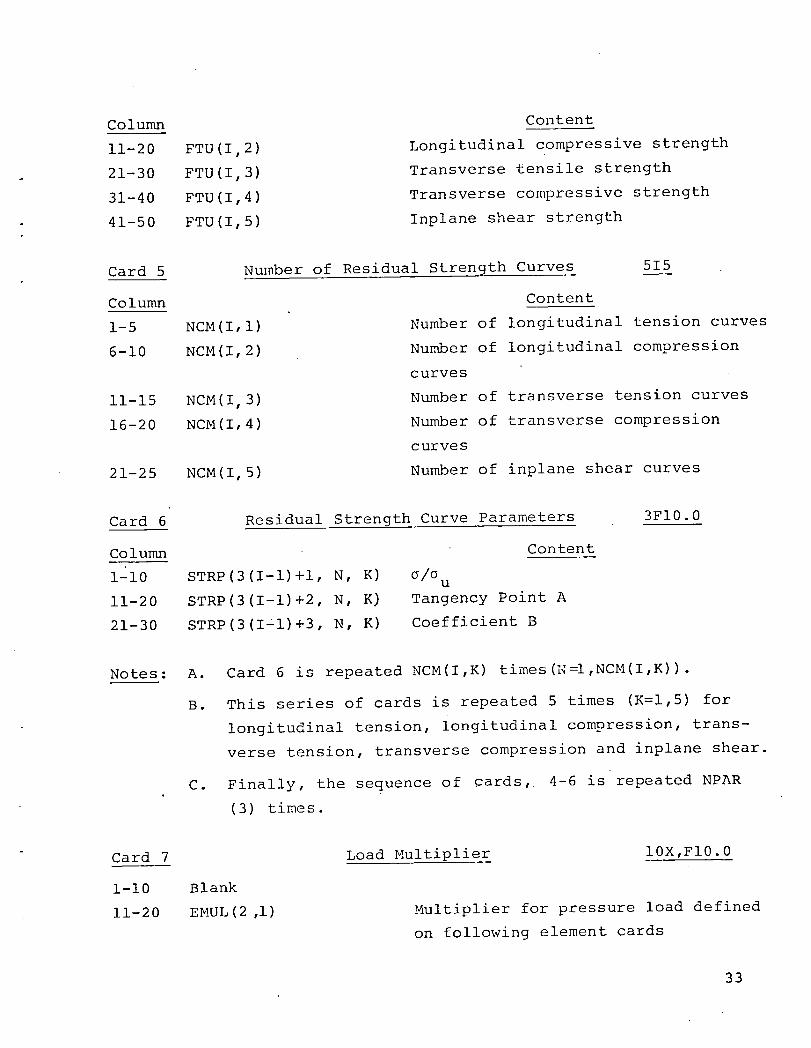
Column Content

11-20 FTU(I,2) Longitudinal compressive strength

21-30 FTU(I 3) Transverse tensile strength

31-40 FTU(I,4) Transverse compressive strength

. 41-50 FTU(I,5) Inplane shear strength

Card 5 Number of Residual Strength Curves 515

Column Content

1-5 NCM(I,I) Number of longitudinal tension curves

6-10 NCM(I,2) Number of longitudinal compression

curves

11-15 NCM(I,3) Number of transverse tension curves

16-20 NCM(I,4) Number of transverse compression

curves

21-25 NCM(I, 5) Number of inplane shear curves

Card 6 Residual Strength Curve Parameters 3FI0.0

Column Content

i-'i0 STRP(3(I-1)+I, N, K) o/o u

11-20 STRP(3(I-I)+2, N, K) Tangency Point A

21-30 STRP(3(I'I)+3, N, K) Coefficient B

Notes: A. Card 6 is repeated NCM(I,K) times(N=l,NCM(I,K)).

B. This series of cards is repeated 5 times (K=I,5) for

longitudinal tension, longitudinal compression, trans-

verse tension, transverse compression and inplane shear.

C. Finally, the sequence of cards, 4-6 is repeated NPAR0

(3) times.

Card 7 Load Multiplier 10X,FI0.0

1-10 Blank

11-20 EMUL(2 ,1) Multiplier for pressure load defined

on following element cards

33

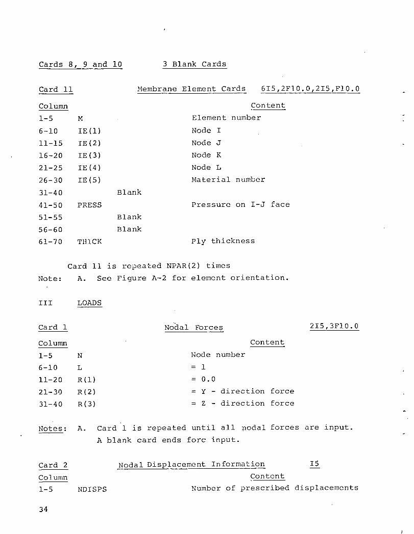
Cards 8, 9 and i0 3 Blank Cards

Card ii Membrane Element Cards 615,2FI0.0,215,FI0.0

Column Content

1-5 M Element number

6-10 IE(1) Node I

11-15 IE(2) Node J

16-20 IE(3) Node K

21-25 IE(4) Node L

26-30 IE(5) Material number

31-40 Blank

41-50 PRESS Pressure on I-J face

51-55 Blank

56-60 Blank

61-70 THICK Ply thickness

Card ii is repeated NPAR(2) times

Note: A. See Figure A-2 for element orientation.

III LOADS

Card 1 N0dal Forces 215,3FI0.0

Column Content

1-5 N Node number

6-10 L = 1

11-20 R(1) = 0.0

21-30 R(2) = Y - direction force

31-40 R(3) = Z - direction force

Notes: A. Card 1 is repeated until all nodal forces are input.

A blank card ends forc input.

Card 2 Nodal Displacement Information I5

Column Content

1-5 NDISPS Number of prescribed displacements

34

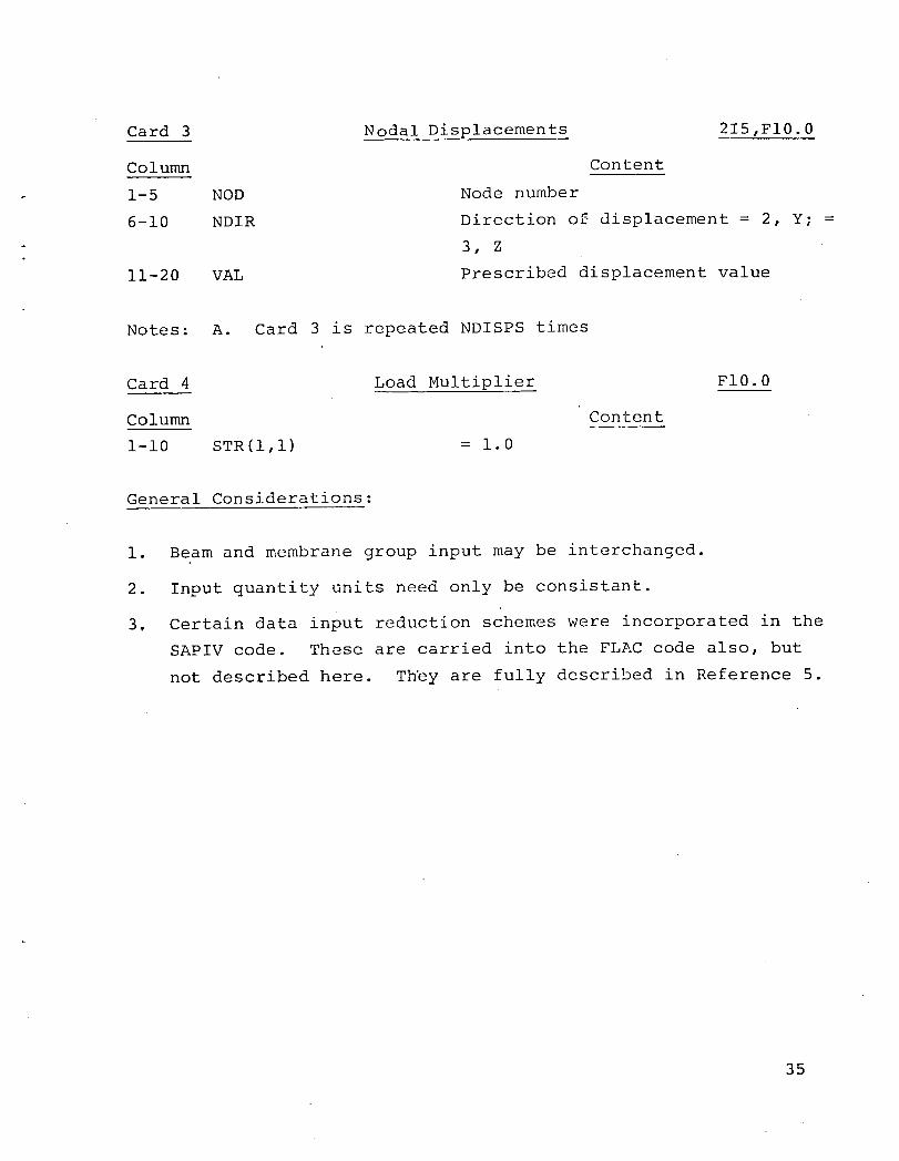
Card 3 Nodal Displacements 215,FI0.0

Column Content

- 1-5 NOD Node number

6-10 NDIR Direction of displacement = 2, Y; =

3, Z

11-20 VAL Prescribed displacement value

Notes: A. Card 3 is repeated NDISPS times

Card 4 Load Multiplier FI0.0

Column Content

1-10 STR(1,1) = 1.0

General Considerations:

i. Beam and membrane group input may be interchanged.

2. Input quantity units need only be consistant.

3. Certain data input reduction schemes were incorporated in the

SAPIV code. These are carried into the FLAC code also, but

not described here. Th%y are fully described in Reference 5.

35

APPENDIX BMEMBRANE AND SHEAR SPRING STRESS ANALYSIS MODEL

The finite element stress analysis model selected for incor-

poration into the fatigue analysis methodology consists of mem-

brane elements and beam elements constrained to act as shear

springs. This particular arrangement was chosen primarily be-

cause of two considerations. First, the model of membrane ele-

ments and shear spring elements yields considerably more economi-

cal results than three-dimensional brick finite element models.

Secondly, the constrained beam elements were selected so as to

alleviate the tedium of developing a specialized shear spring

element. Both of the element types used and the various routines

needed for their development were adapted from the SAP IV analy-

sis code (ref. 5).

The basic model of a laminated composite plate is depicted

in figure B-I. Since membrane elements have no bending or out of

plane stiffness, the plate modeled must be balanced and mid-plane

symmetric. This removes the possibility of any material induced

bending. In addition, no bending may be applied to the model

through the various loadings available. Due to the restriction

that the laminate be balanced and mid-plane symmetric, no shear-

ing forces may exist there. Hence, the interface at the mid-

plane need not be modeled.

In the model as described, the only degrees of freedom which

are allowable are in-plane translations. Thus, all other compo-

nents, three rotations and the out of plane translations, must be

constrained out of the model. The constraint upon nodal rotations

in the model causes the beam elements to deflect as shown in fig-

ure B-2. In order that static equilibrium be satisfied, the mo-

ment, M, caused by the shearing forces, F, is reacted by con_

straint forces at the nodes.

In figure B-2, the relationship between ply thickness, shear

modulus and beam flexural moment of inertia is also depicted. The

relation for "I" given in the figure must be used in the finite

element model so the interlaminar element will have the proper

force-displacement relationship. The area "A" used in the flexural

36

inertia computation is defined in figure B-3. The beam, connected

to a node, must carry the interlaminar shear forces corresponding

to some portion of the membrane elemental areas also connected to

that node. In the figure there are four membranes at node in

" question, thus the area utilized in the flexural inertia computa-

tion corresponds to one-fourth the sum of the areas of the mem-

branes. Using the method depicted in the figure, a consistent

allocation of shear areas is obtained.

37

APPENDIX CQUASI THREE-DIMENSIONAL FINITE ELEMENT ANALYSIS

To verify the membrane and shear spring analysis model, com-

parisons were made with a finite difference solution and with a

quasi three-dimensional analysis. The quasi three-dimensional

analysis was supplied by Dr. G. L. Roderick, NASA Langley. This

appendix contains a brief description of the quasi three-dimen-

sional formulation. The finite element model used in implement-

ing the quasi three-dimensional model is also described.

The quasi three-dimensional finite element model is based

upon the same elasticity formulation as the finite difference

solution of reference 6. The model considers the stress and

strain state in an infinite coupon to be independent of the coor-

dinate in the infinite direction (X-direction in the following

and in the comparisons in the text).

The displacement field, corresponding to these stress and

strain states, for a balanced symmetric laminate are:

u = _ X + U (y,z)x x x

u = u (y,z) (c-l)y y

uz = uz (y,z).

These displacement fields can easily be seen to yield six strain

components which are independent of X.

The finite element grid used in the comparisons is shown in

figure C-I. The model has a ply aspect ratio (b/ho) of 32. Eachelement in the model is an eight noded quadrilateral with three-

degrees of freedom per node. The nodes are situated at the four

vertexes and at the four mid-sides. The material properties used

in the analysis were previously listed in table i.

38

REFERENCES

i. McLaughlin, P.V., Jr., Kulkarni, S.V., Huang, S.N., and

Rosen, B.W., "Fatigue of Notched Fiber Composite Laminates,

. Part I: Analytical Model," NASA CR-132747, March 1975.

2. Kulkarni, S.V., McLaughlin, P.V., Jr., and Pipes, R.B.,

"Fatigue of Notched Fiber Composite Laminates, Part II:

Analytical and Experimental Evaluation," NASA CR-145039,

April 1976.

3. Ramkumar, R.L., Kulkarni, S.V., and Pipes, R.B., "Evalua-

tion and Expansion of an Analytical Model for Fatigue of

Notched Composite Laminates," NASA CR-145308, March 1978.

4. Pifko, A., Armen, H., Jr., Levy, A., and Levine, H., "PLANS--

A Finite Element Program for Nonlinear Analysis of Structures,

Volume II - Users Manual," NASA CR-145244, May 1977.

5. Bathe, K., Wilson, E.L., and Peterson, F.E., "SAP IV, A

Structural Analysis Program for Static and Dynamic Response

of Linear Systems," EERC-73-11, June 1973.

6. Pipes, R.B., and Pagano, N.J., "interlaminar Stresses in

Composite Laminates Under Uniform Axial Extension," Journal

of Composite Materials, October 1970.

7. Hashin, Z., "Failure Criter_n for Uni-Directional Composites

in Print, Journal of Applied Mechanics, 1980.

8. Harris, B., "Fatigue and Accumulation of Damage in Reinforced

Plastics," Composites, Vol. 8 No. 4, October 1977, pp. 214-220.

9. Advanced Composites Design Guide, 3rd Edition, January 1973.

39

Table i. Elastic Constants for Edge Effect Problems

Eli = 138 GPa

E22 = 14.5 GPa

GI2 = 5.86 GPa

912 = 0.21

Table 2. Elastic Constants for Notched Plate Problem

Ell = 139 GPa

E22 = 12.0 GPa

GI2 = 5.20 GPa

_12 = 0.38

4O

Table A-I. Failure Criteria

Tensile Fiber Mode

+°ll = °A

Compressive Fiber Mode

Oll = -OA

Tensile Matrix Mode

1 2 1 2+2" 022 + --_o12 = 1

oT T

Compressive Matrix Mode

OT 2 1 2 1 2 =1 [(____)- i] 022 + ---7022 + --_O12 1

oT 4T T

Tensile Interlaminar Mode

1 2 1 2 2033 + --_ (O13 + 023) = 1+2

oT T

Compressive Interlaminar Mode

i [(____)- i] o + 1 1 132 2_ 02. `OT 33 4T2033 + --2T(0 + ) = 1

41

Table A-I. Failure Criteria (Continued)

where

+_A = axial tensile strength

_A = axial compressive strength

_T+ = transverse tensile strength

aT = transverse compressive strength

T = shear strength

w

42

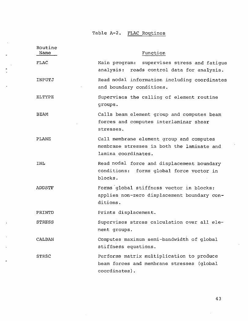
Table A-2. FLAC Routines

RoutineName Function

FLAC Main program: supervises stress and fatigue

analysis: reads control data for analysis.

INPUTJ Read nodal information including coordinates

and boundary conditions.

ELTYPE Supervises the calling of element routine

groups.

BEAM Calls beam element group and computes beam

forces and computes interlaminar shear

stresses.

PLANE Call membrane element group and computes

membrane stresses in both the laminate and

lamina coordinates.

INL Read nodal force and displacement boundary

conditions: forms global force vector inblocks.

ADDSTF Forms global stiffness vector in blocks:

applies non-zero displacement boundary con-

ditions.

PRINTD Prints displacement.

STRESS Supervises stress calculation over all ele-

ment groups.

CALBAN Computes maximum semi-bandwidth of global

stiffness equations.

STRSC Performs matrix multiplication to produce

beam forces and membrane stresses (global

coordinates).

43

RoutineName Function

ELT2, TEAM, Beam element group: input geometric and

NEWBM material properties: form elemental stiff-

ness and stress recovery matrices.

ELT3A4, Membrane element group: input geometric

PLNAX, ELAW, and material properties: form elemental

QUAD, FORMB, stiffness and stress recovery matrices.

VECTOR, CROSS, DOT

SOLEQ Supervises the static solution: calls so-

lution routine, displacement print routine

and stress recovery routines.

SESOL Performs the solution for the displacementvector.

ADSTF2 Add negative elemental stiffness matrices

to the existing global stiffness matrix.

RESET Saves information corresponding to a fatigue

load stress distribution for use with a

later fatigue cycle increment and retrieves

information at the following fatigue cycle

increment.

FAIL Computes least failure loads using failure

criterion.

ROTR Rotates membrane stresses from laminate

coordinates to lamina coordinates

STREN Computes coefficients in failure criterion.

PARAM Updates elemental strengths.

PREFAL Updates elemental failure vector and checks .

if element has failed previously.

RESTRT Saves data for solution restart and retrieves

data when restarting.

44

RoutineName Function

PRINT Prints fatigue analysis parameters.

ERROR Terminates execution if storage is

insufficient

45

X Loading Direction

o_

b- 1.14

LX

Figure i. Edge Effect Finite Element Model

25

b =

[+45]S he "_._ ;re_e_t-- -. _

20 -----------

Study---------Finite Difference (Ref. 6)

15Io

oco• _

_ _ .--------_--__ _ __-<_0 , _---v ! _" "m?

0.0 0.2 0.4 0.6 0.8 1.0Yb

Figure 2. Comparison of Present Solution with Finite

Difference Solution for [±45]s Edge EffectProblem

47

30b

[±30/90] s _- = 32 -30/90 Interfaceo

z- 1

20 -- ho

i0 --l

° ¢!

0 -I__ _XZ Present Study -_\_

Oyz Present Study "\ /\-i0 -- o Quasi 3-D \

xz \o Quasi 3-Dyz

-20 --

-30 I I I 10 0.2 0.4 0.6 0.8 1.0 .

Y

Figure 3. Comparison of Present Solution with Quasi 3-DSolution for Interlaminar Shear Stresses at

Z/ho=l, in a [±30/90] s Edge Effect Problem

48

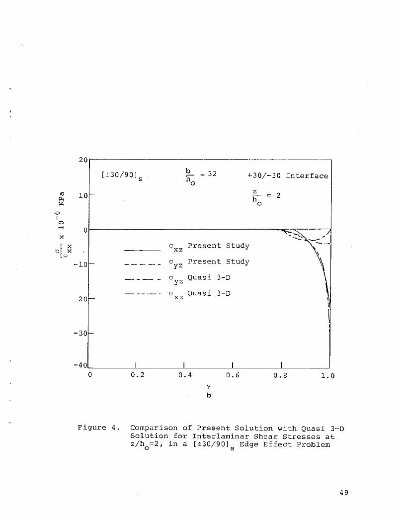
2O

b - 32 +30/-30 Interface[±30/90]s ho

10 - z__ = 2_ hM 0

Io

_ 0N "

blw_ _xz Present Study

-10-- _yz Present Study

Quasi 3-Dyz

.... _ Quasi 3-D-20-- xz

-30 --

-4O I I I I0 0.2 0.4 0.6 0.8 1.0

Y

Figure 4. Comparison of Present Solution with Quasi 3-DSolution for Interlaminar Shear Stresses at

Z/ho=2, in a [±30/90] s Edge Effect Problem

49

3.0

b[±30/90]S _-- = 32 ,4

O

2.5-

2.0 --

+30/-30 Present Study

1.5- -30/90 Present Study Ii

i!+30/-30 Quasi 3-D

-30/90 Quasi 3-D II

1.0- !I

II

0.5- ]

° \N \ \\

os ux -0.5-- I l\I

\\ [-i.0-- \\\ I

'\J-1.5-- I

\-2.0-- \,1

\ !\J

-2.5 '1 I I 10.0 0.2 0.4 0.6 0.8 1.0

Y

b

Figure 5. Comparison of Present Solution with Quasi 3-DSolution for Interlaminar Normal Stresses in a

[±30/90] Edge Effect Problems

50

i0

z _ 1 -30/90 Interface[-+30/90]s ho0 -_

Io -10 -

UXZ× b

<_ _---= 32× .... yz o

-20 -O

-30 I I i !

0.0 0.2 0.4 y 0.6 0.8 1.0b

- Figure 6. Interlaminar Shear Stresses Predicted by thePresent Analysis at z/ho=l with Beam StiffnessDivided by Four [±30/90] Edge Effect Problems

51

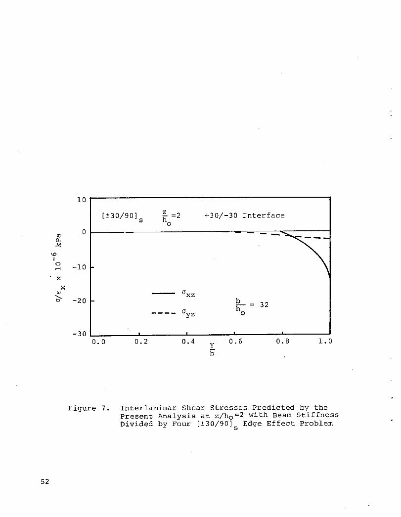
10

z=2 +30/-30 Interface[±30/90] s

0

0 -- --- -.....__

kOIo

-lO

MO_ .........- UXZ

-20 b- 32

Oy z ho

-30 l , l i0.0 0.2 0.4 0.6 0.8 1.0Y

b

Figure 7. Interlaminar Shear Stresses Predicted by thePresent Analysis at z/ho =2 with Beam Stiffness

Divided by Four [±30/90] s Edge Effect Problem

52

1.27cm

£5

Figure 8. Notched Laminate Finite Element Model

8.0

0° PliesLoading

8 Direction 45o_p&y_6.0

-4_.s°._.

- 1.05 [/]L02-+45"sr4.0 c

°I8

2.0

0

-2.0 I I I0.0 40 80 120 160

e, Degrees

Figure 9. Circumferential Stress Near the Notch in a[02/-+45]s Notched Plate

54

6.0

8 LoadingDirection

5.09 = 84.375°

4.0 0° Plies

45° Ply

_ 30 -4so._ly__D " •

[02/-+45] s

2.0

1. o _,-,,, _

0.0 I I I1.0 2.0 3.0 4.0 5.0

rc

Figure 10. Circumferential Stresses at 9 = 84.375 ° in a

[02/±45] s Notched Plate

55

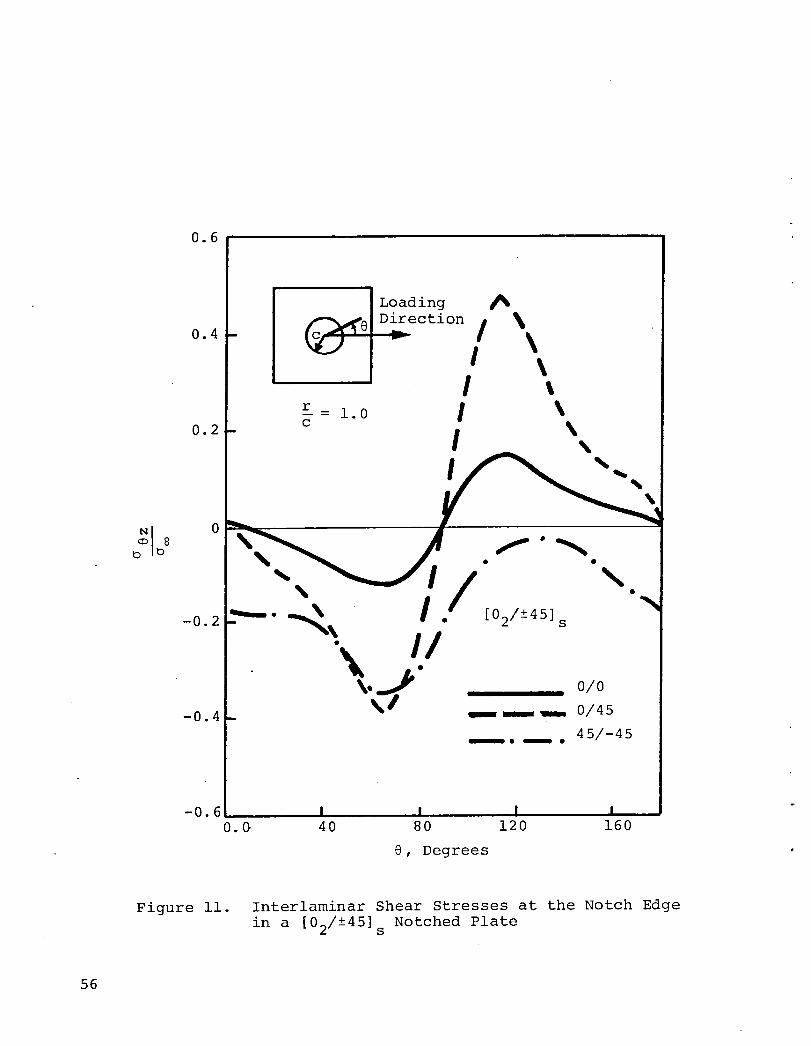
0.6

Loading

0.4 - _ Direction/ ,

\r- 1.0 /0.2- c \\

-0.6 I I I I0.0 40 80 120 160

O, Degrees

Figure ii. Interlaminar Shear Stresses at the Notch Edgein a [02/±45]s Notched Plate

56

0.i

e = 67.5°

0/0 Interface

0

[02/+45]s_ 8

Loading-0.i _ Direction

'0.2 I I I1.0 2.0 3.0 4.0 5.0

rc

Figure 12 Interlaminar Shear Stresses at 8 = 67 5°' 0/0 Interface, of a [02/±45] s Notched Plate

57

0.1

0

6 _ Loading-0.1 v Direction

NIo8_Do

-0.2 e = 67.5°

0/45 Interface

[02/-+45] s-0.3

-0.4 I I I1.0 2.0 3.0 4.0 5 0

rc

Figure 13 Interlaminar Shear Stresses at 8 = 67 5°• • F

0/45 Interface, in a [02/+--45] s Notched Plate

58

0.i

.-A-0 1 I K-I_8 -- Loading

• _ "- Direction

N188 = 67.5 °

-0.2

45/-45 Interface

[02/-+45]s-0.3 -

-0.4 I I I.,1.0 2.0 3.0 4.0 5.0

rc

Figure 14 Interlaminar Shear Stresses at 8 = 67 5°• • F

45/-45 Interface, in a [02/-+45] s Notched Plate

59

-0.2 I1.0 2.0 3.0 4.0 5.0

rc

Figure 15. Radial Stresses at 8 = 84.375 in a [02/±45]sNotched Plate

60

0.8

A 8 = 84.375 °

i _@ Loading0.6 _ Direction

I0° Plies

0.4

k 45° Ply

-45 Plyo

0.2 . _• _

°p_ g

[02/+-45] s0.0

I S-0.2 S S

. f

-0 4 - J0'

-0.6 I I I1.0 2.0 3.0 4.0 5.0

rc

Figure 16. In-Plane Shear Stresses at 8 = 84.375 ° in a

[02/-+45] s Notched Plate

61

OhtO

1500

-_ _ _ o.o,o.1

_u

i000 -

¢

_q

500 -'0-,-IO_

0 I I I I I I0 1 2 3 4 5 6 7

Log (N)

Figure 17. Lamina Residual Axial Tensile Strength

! i • * t

1500

o

0oor_

500

0 I I I I I I

0 1 2 3 4 5 6 7

Log (N)

o__o

Figure 18. Lamina Residual Axial Compressive Strength

50

40.°u

30 -

4-)

_)14

T.Q

,_ 20 -nJm'0-,-I

lO

0.0 I ! I I i l

0 l 2 3 4 5 6 7

Log (N)

Figure 19. Lamina Residual Transverse Tensile Strength

! I • r i

150 _

i00 -

4J_D

4J•5q

50 "-4

O

0 I I I I I I0 1 2 3 4 5 6 7

Log (N)

Figure 20. Lamina Residual Transverse Compressive Strength

80

_

0 u

4O

20

0 I I I I I I0 Z 2 3 4 5 6 7

Log (N)

Figure 21. Lamina Residual Shear Strength

First 0° Ply Second 0 ° Ply

Loading Direction

45° Ply -45° Ply

o%

Figure 22. In-Plane Damage at 179 MPa, N = i, in a [02/+45]s Notched Plate

co

Loading Direction

0/45 Interface 45/-45 Interface

Figure 23. Interlaminar Damage at 179 MPa, N = l, in a [02/±45] s Notched Plate

First 0° Ply Second 0° Ply

Loading Direction

45 ° Ply -45 ° Ply

Figure 24. In-Plane Damage at 226 MPa, N = i, in a [02/-+45]s Notched Plate

-4O

Loading Direction/

0/45 Interface 45/-45 Interface

Figure 25. Interlaminar Damage at 226 MPa, N = l, in a [02/±45] s Notched Plate

First 0 ° Ply Second 0 ° Ply

Loading Direction

45 ° Ply -45 ° Ply

Figure 26. In-Plane Damage at Fatigue Load. 103 MPa, N = i000, in a [02/±45] sNotched Plate

Loadinq Direction

0/45 Interface 45/-45 Interface

Figure 27. Interlaminar Damage at Fatigue Load, 103 MPa, N = i000, in a [02/±45]sNotched Plate

I F . . J, I

First 0 ° Ply Second 0 ° Ply

Loading Direction

45 ° Ply -45 ° Ply

uo

Figure 28. In-Plane Damage at 186 MPa, N = i000, in a [02/-+45] s Notched Plate

Loading Direction

0/45 Interface 45/-45 Interface

Figure 29. Interlaminar Damage at 186 MPa, N & 1000, in a [02/±45]s Notched Plate

First 0 ° Ply Second 0° Ply

Loading Direction

45° Ply -45 ° Ply

Figure 30. In-Plane Damage at the Fatigue Load, 103 MPa, N = I0 000, in a [02/±45]stNotched Plate

-4

Loading Direction

0/45 Interface 45/-45 Interface

Figure 31. Interlaminar Damage at Fatigue Load, 103 MPa, N = 10,000, in a [02/±45] sNotched Plate

! e _ • k •

First 0° Ply Second 0° Ply

Loadinq Direction

45° Ply -45° Ply

_ Figure 32. In-Plane Damage at 208 MPa, N = i0,000, in a [02/±45]s Notched Plate

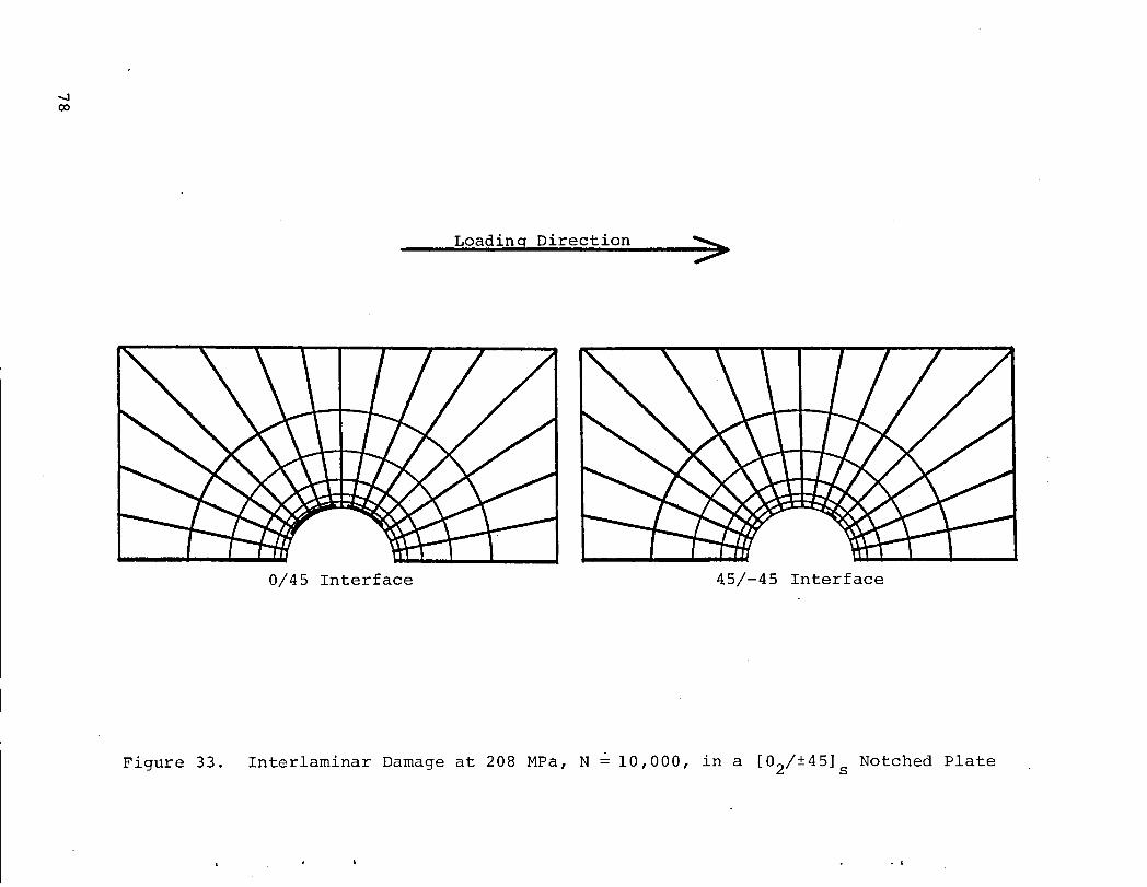
oo

Loadinq Direction

0/45 Interface 45/-45 Interface

Figure 33. Interlaminar Damage at 208 MPa, N = 10,000, in a [02/±45] s Notched Plate

L . ! j

Stat:lc Ans_lys_s ; N=]

L]_nput laminae propert:ies, boundary conditions, 3oads]

- _ iObtain e]astJc so]ut_on for unit load]

, Use appropriate failure criteria to determine the fa_]ureU[loads for different fa_[lure modes and the corresponding

failure locations....... l ..................

Check for the least fafilure ]oad to determine ]"imminent failure(s) and the corresponding location(s) ]-I checktosee_ the_ea_t_a_e_o_ _II e):ceeds the ma_:i_um fatigue load I

failure _. responding to the |

f_rst t_me it _s |1_ e_.c_edea l

Fatigue :gas [lur el [of notched • Check for laminate failure_

I_nt strength ]] and 3.iretiree ---- _PrintIstiffness matr_ce Strength

to account for (N)faJ[lure(s) [|

] For E=N4AN, restartusing data corte-s/bonding 1o max.]4odify the g3obal stiffness

" " fatigue loadmatr_r, to account for all changes

- II Chan_e strength ]values used _n the]fai[lure criteria

Figure A-I. Flow Chart of Computerized Fatigue Analysis Methodology

79

coo

Log AStatic Strength

l I i

_ Fatigue Stress____ I

_ Statlc Strength .80 .50 _0 _

-Mm

Residual Strength = Static Strength - (LogN-LogA) 2B

i

Log N

Figure A-2. Form of Lamina Residual Strength Data

X,3

e-_ Zv

Y 1

Figure A-3. FLAC Coordinate System

81

J

i 3

1

Figure A-4. Beam Node and Force Definition

82

, t I I -,, I

Membranes

II

Plan-Form

Shear Springs

Through the ThicknessSection

Figure B-I. Membrane and Shear Spring Model of a Balanced SymmetricLaminated Plate with Ten Plies

oo

FF _-e--4m- "_v

I--i T I -7

: I T i ,I I I! I I I

I I

/ / tply I I I

" J_I !

M F

Ft31y FtplyA - A =12EI AG

AGt21yI - 12E

Figure B-2. Shear Spring Stiffnesses

Area Used in Reduced Flexural

Inertia Computation./

/ 8

Figure B-3. Area Used in Determining ShearSpring Stiffness

85

00o_

z -3ho

z_= 2ho

z -1ho

z---=0

ho y=0 y=b

bY=y y=b

Figure C-I. Quasi Three-Dimensional Finite Element Analysis Model Geometry

NASAContractor Report 159119NASI-15411

DISTRIBUTIONLIST

No,

o CopiesNASALangley Research CenterHampton, VA 23665Attn: Report & Manuscript Control Office, Mail Stop 180A 1

'. Structures Laboratory, USARTL(AVRADCOM),Mail Stop 266 2G. L. Roderick, Mail Stop 188E 21

"- NASAAmes Research CenterMoffett Field, CA 94035Attn: Library, Mail Stop 202-3 1

Headquarters, USARTL(AVRADCOM),Mail Stop 207-I 2Aeromechanics Lab, USARTL(AVRADCOM),Mail Stop 215-I 2

NASAHugh L. Dryden Flight Research CenterEdwards, CA 93523Attn: Library 1

NASAGoddard Space Flight CenterGreenbelt, MD 20771Attn: Library 1

Jet P.ropulsion Laboratory4800 Oak Grove DrivePasadena, CA 91103Attn: Library, Mail Stop 111-113 1

NASALyndon B. Johnson Space CenterHouston, TX 77058Attn: JM6/Library 1

John F. Kennedy Space Center, NASAKennedy Space Center, FL 32899Attn: Library, IS-DOC-IL 1

NASALewis Research Center21000 Brookpark RoadCleveland, OH 44135

' Attn: Library, Mail Stop 60-3 1Propulsion Lab, USARTL(AVRADCOM),Mail Stop 500-317 2

NASAGeorge C. Marshall Space Flight CenterMarshall Space Flight Center, AL 35812

_ Attn: Library, AS61L 1

87

DISTRIBUTIONLIST 2NO.

CopiesNational Aeronautics and Space AdministrationWashington, DC 20546Attn: RTM-6 1

University of WisconsinDepartment of Engineering MechanicsMadison, WI 53706Attn: Professor R. E. Rowlands 1

United Aircraft CorporationPratt & Whitney AircraftEast Hartford, CT 06118Attn: Dr. T. A. Cruse, Scientific Analysis Group 1

University of WyomingDepartment of Mechanical EngineeringLarmie, WY 82070Attn: Professor Donald F. Adams 1

University of Minnesota107 Aeronautical Engineering BuildingMinneapolis, MN 55455Attn: Professor Phil Hodge 1

Northrop CorporationAircraft Division3901W. BroadwayHawthorne, CA 90250Attn: Glen C. Grimes, Engineering Specialist,

Structures R&T, Dept. 3780/62 1

Kedwork, Kawa& Associates, Ltd.400 Kelvin BoulevardWinnipeg, ManitobaCanada R3P OJ2Attn: Dr. Keith T. Kedwork 1

McDonnell-Douglas CorporationP. O. Box 516St. Louis, MO 63166Attn: Dr. Michael P. Renieri, Bldg. 34, Post 350 1

Dr. Gary D. Renieri, Bldg. 106, Level 4, Post C-5 1

Department of the NavyOffice of Naval ResearchArlington, VA 22217Attn: Dr. Nicholas Perrone, Director, Structural Mechanics Prog. 1

88

DISTRIBUTIONLIST 3No,

CopiesNational Science FoundationWashington, DC 20550Attn: Dr. Clifford J. Astill, Solid Mechanics Program 1

Air Force Flight DynamicsLaboratoryWright-Patterson AFB, OH 45433

" Attn: Dr. George P. Sendeckyj, Structures Division 1_' Dr. J. C. Halpin 1

Air Force Materials LaboratoryWright-Patterson AFB, OH 45433Attn: Dr. J. M. Whitney, Nonmetallic Materials Division 1

Dr. H. T. Hahn, Nonmetallic Materials Division 1Dr. N. J. Pagano, MBM 1Dr. S. Tsai, MBM 1

University of DelawareDepartment of Mechanical & Aerospace Engineering107 Evans HallNewark, DE 19711Attn: Dr. R. Byron Pipes 1

Battelle-Columbus Laboratories505 King AvenueColumbus, OH 43201Attn: Dr. EdmundF. Rybicki 1

Lawrence Livermore LaboratoryUniversity of CaliforniaLivermore, CA 94550Attn: Dr. S. Kulkarni 1

liT Research InstituteI0 West 35 StreetChicago, IL 60616Attn: Dr. I. M. Daniel, Manager 1

-., General Dynamics CorporationFort Worth, TX 76101

- Attn: M. E. Waddoups 1

McDonnell-Douglas CorporationMcDonnell-Douglas Astronautics Company5301 Bolsa AvenueHuntington Beach, CA 92647

- Attn: Dr. Longin B. Greszczuk 1

89

DISTRIBUTIONLIST 4No.

CopiesUniversity of lllinoisDepartment of Theoretical and Applied MechanicsIOOETalbot LaboratoryUrbana, IL 61801 1 -

Lockheed Aircraft CorporationLockheed-California CompanyP. O. Box 551 "'Burbank, CA 91520Attn: Larry R. Markham, Dept. 7572, Bldg. 63, Plant A1 1

The Boeing CompanyP. O. Box 3707Seattle, WA 98124Attn: John McCarty, Mail Stop 30-01 1

Applied Technology Laboratory, USARTL(AVRADCOM)Fort Eustis, VA 23604Attn: J. Robinson/SAVDL-EU-SS 1

A. J. Gustafson 1

Department of the ArmyU.S. Army Materials & Mechanics Research CenterWatertown, MA 02172Attn: Dr. E. Lenoe 1

Dr. J. Perkins 1

Picatinny ArsenalMaterials Engineering Laboratory, Bldg. 183Dover, NJ 07801Attn: Charles Wright 1

Naval Air Development CenterWarminster, PA 18974Attn: Dr. Jim Huang, Code 3033 1

NASAScientific & Technical Information Facility6571 Elkridge Landing Road ,--Linthicum Heights, MD 21090 30

plus original

9O