AAS 16-201

ABSOLUTE NAVIGATION PERFORMANCE OF THE ORIONEXPLORATION FLIGHT TEST 1

Renato Zanetti∗, Greg Holt†, Robert Gay‡, Christopher D’Souza§,and Jastesh Sud ¶

Launched in December 2014 atop a Delta IV Heavy from the Kennedy Space Center, theOrion vehicle’s Exploration Flight Test-1 (EFT-1) successfully completed the objective tostress the system by placing the un-crewed vehicle on a high-energy parabolic trajectoryreplicating conditions similar to those that would be experienced when returning from an as-teroid or a lunar mission. Unique challenges associated with designing the navigation systemfor EFT-1 are presented with an emphasis on how redundancy and robustness influenced thearchitecture. Two Inertial Measurement Units (IMUs), one GPS receiver and three baromet-ric altimeters (BALTs) comprise the navigation sensor suite. The sensor data is multiplexedusing conventional integration techniques and the state estimate is refined by the GPS pseu-dorange and deltarange measurements in an Extended Kalman Filter (EKF) that employsUDU factorization. The performance of the navigation system during flight is presented tosubstantiate the design.

INTRODUCTION

The Orion vehicle, designed to take men back to the Moon and beyond, successfully completed its firstflight test, EFT-1 (Exploration Flight Test-1), on December 5th, 2014. The main objective of the test wasto demonstrate the capability of re-enter into the Earth’s atmosphere and safe splash-down into the PacificOcean. This un-crewed mission completes two orbits around Earth, the second of which is highly ellipticalwith an apogee of approximately 5908 km, higher than any vehicle designed for humans has been since theApollo program. The trajectory was designed in order to test a high-energy re-entry similar to those crewswill undergo during lunar missions. The mission overview is shown in Figure 1.

The first of the two orbits starts with the conclusion of the first upper stage burn (SECO1); towards the endof the first orbit, the upper stage ignites again to raise the apogee, the conclusion of this second upper stageburn (SECO2) places Orion on its final highly elliptical orbit. Following apogee the Orion capsule separatesfrom the upper stage, from this moment on Orion is responsible for its own onboard Guidance, Navigation,and Control (GN&C) to safely take the vehicle to splash-down in the Pacific Ocean; although the absolutenavigation system was active during the entire flight.

The objective of this paper is to document the performance of the absolute navigation system during EFT-1, which relies on the classic extended Kalman filter (EKF) [1]. A prior version of this work introduced thenavigation design [2], while pre-flight simulation performance was shown in Ref. [3]. The UDU factorizationas introduced by Bierman is employed in the filter design [4], and measurements are included as scalars

∗GN&C Autonomous Flight Systems Engineer, Aeroscience and Flight Mechanics Division, EG6, 2101 NASA Parkway. NASA JohnsonSpace Center, Houston, Texas 77058.†Flight Dynamics Engineer, Flight Operations Directorate, CM55, 2101 NASA Parkway. NASA Johnson Space Center, Houston, Texas77058.‡GN&C Autonomous Flight Systems Engineer, Aeroscience and Flight Mechanics Division, EG6, 2101 NASA Parkway. NASA JohnsonSpace Center, Houston, Texas 77058.§GN&C Autonomous Flight Systems Engineer, Aeroscience and Flight Mechanics Division, EG6, 2101 NASA Parkway. NASA JohnsonSpace Center, Houston, Texas 77058.¶Systems Engineer Sr, Lockheed Martin Space Systems Company, M/S B3003, P.O. Box 179, Denver, CO 80201

1

https://ntrs.nasa.gov/search.jsp?R=20160001440 2018-06-03T23:33:09+00:00Z

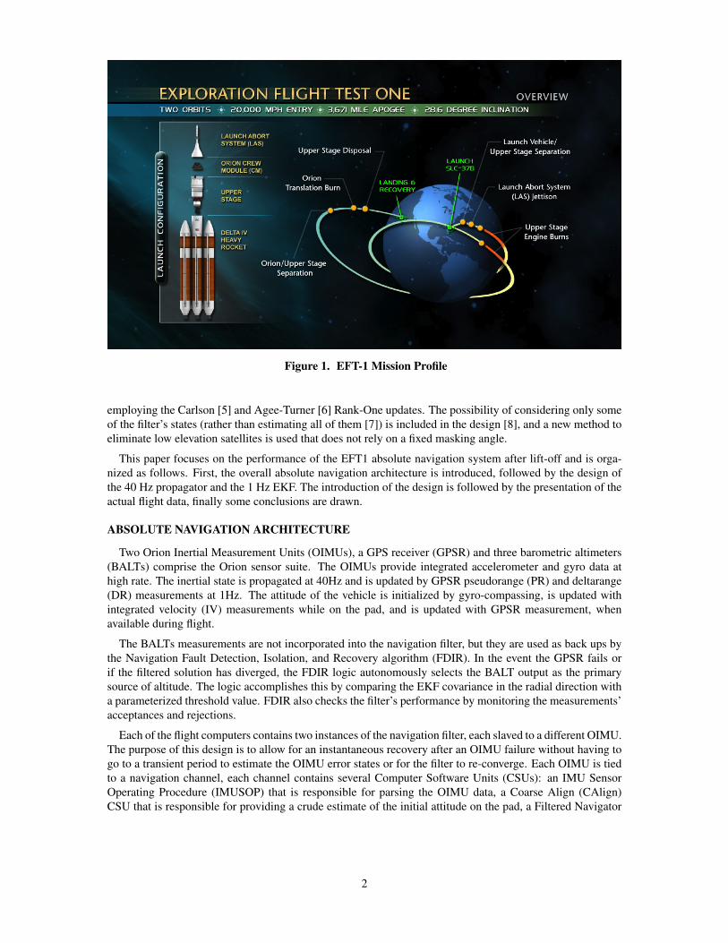
Figure 1. EFT-1 Mission Profile

employing the Carlson [5] and Agee-Turner [6] Rank-One updates. The possibility of considering only someof the filter’s states (rather than estimating all of them [7]) is included in the design [8], and a new method toeliminate low elevation satellites is used that does not rely on a fixed masking angle.

This paper focuses on the performance of the EFT1 absolute navigation system after lift-off and is orga-nized as follows. First, the overall absolute navigation architecture is introduced, followed by the design ofthe 40 Hz propagator and the 1 Hz EKF. The introduction of the design is followed by the presentation of theactual flight data, finally some conclusions are drawn.

ABSOLUTE NAVIGATION ARCHITECTURE

Two Orion Inertial Measurement Units (OIMUs), a GPS receiver (GPSR) and three barometric altimeters(BALTs) comprise the Orion sensor suite. The OIMUs provide integrated accelerometer and gyro data athigh rate. The inertial state is propagated at 40Hz and is updated by GPSR pseudorange (PR) and deltarange(DR) measurements at 1Hz. The attitude of the vehicle is initialized by gyro-compassing, is updated withintegrated velocity (IV) measurements while on the pad, and is updated with GPSR measurement, whenavailable during flight.

The BALTs measurements are not incorporated into the navigation filter, but they are used as back ups bythe Navigation Fault Detection, Isolation, and Recovery algorithm (FDIR). In the event the GPSR fails orif the filtered solution has diverged, the FDIR logic autonomously selects the BALT output as the primarysource of altitude. The logic accomplishes this by comparing the EKF covariance in the radial direction witha parameterized threshold value. FDIR also checks the filter’s performance by monitoring the measurements’acceptances and rejections.

Each of the flight computers contains two instances of the navigation filter, each slaved to a different OIMU.The purpose of this design is to allow for an instantaneous recovery after an OIMU failure without having togo to a transient period to estimate the OIMU error states or for the filter to re-converge. Each OIMU is tiedto a navigation channel, each channel contains several Computer Software Units (CSUs): an IMU SensorOperating Procedure (IMUSOP) that is responsible for parsing the OIMU data, a Coarse Align (CAlign)CSU that is responsible for providing a crude estimate of the initial attitude on the pad, a Filtered Navigator

2

(FiltNav) CSU that is responsible for multiplexing the OIMU data with the GPS updates and an InertialNavigator (INRTLNAV) CSU that is responsible for maintaining an un-aided (OIMU-only) state. INRTLNAVand FiltNav have counterparts on the 1Hz side. The Inertial Navigator Gravity (InrtlNavGrav) and ExtendedKalman Filter (EKF) CSUs on the 1Hz side provide a higher-order gravity estimate to INRTLNAV and stateupdates to FiltNav, respectively.

The outputs of the two channels are received by Navigation FDIR (NAVFDIR) CSU which selects theprimary state. The NAVFDIR scheme relies on the IMUFDIR outputs and performs additional tests on thefiltered solution. One of the checks it relies on is the percentage of PR/DR measurements being accepted byeach channel.

Prior to launch the filter is initialized with the coarse align attitude and an inertial position derived fromthe current time and the coordinates of the pad. This pre-launch navigation phase is called fine align and theonly measurement active in this mode is integrated velocity, which is a pseudo-measurement consisting of azero change of Earth-referenced position over a 1 second interval. The GPSR measurement are not availableduring fine align. The main purpose of fine align is to better estimate the attitude and the IMU states.

The ascent phase is divided in two parts, the first when GPSR measurements are not enabled, and the secondwhen they are. The only difference between Fine Align and Ascent Without GPS is that the IV measurementprocessing flag is set to zero in the latter. The maximum number of processable measurements is set to 12which is a large enough number to obtain very good performance while keeping the throughput reasonablylow. To avoid possible transient issues the very first PR measurement is not processed. After a long blackoutthe covariance becomes very large and the nonlinearity of the DR measurement creates convergence issues.Through numerical simulation it was determined that allowing for multiple PR (∼30s) to be processed beforeincorporating a DR mitigates this issue because the PRs shrink the uncertainty before DRs are introduced.If a satellite is not present for a single cycle, the counters are not reset and if the satellite comes back isimmediately used as a measurement. If the satellite is absent for more than a cycle the counters are reset.

The GPSR provides an estimate of the PR variance together with the measurement. The EKF uses thisvariance estimate together with PR variance floor parameter which limits the minimum value of PR mea-surement variance used in incorporating the measurement into the filter. Underweighting is applied when theestimated measurement has an uncertainty greater than 100ft. One of the EFT-1 mission goals was to testGPSR clock stability, clock filter state restarts, and high altitude GPS processing.

GPSR measurements are processed throughout the orbit phase and during entry when available. A GPSblackout was expected and experienced during entry. In order to process latent GPS measurements the EKFnecessitates to back-propagate its current state estimate to the measurement time. This task is made possibleby a 4Hz buffer of OIMU data provided to EKF by FiltNav. When accelerating fast under the chutes duringentry, the attitude dynamics are not accurately represented by the 4Hz IMU buffer. Therefore PR and DR areinhibited above a certain angular velocity.

A major frame is a 1 Hz cycle and is denoted by a capital letter (A, B, C, etc.) individual EKF calls aredenoted by their major frame. A minor frame is a 40 Hz cycle and is denoted by a number from 0 to 39,individual FiltNav calls are denoted by both their major and minor frame (A0, A1, A39, B0, etc.). FiltNavreceives EKF data at minor frame 0, that is to say that FiltNav B0 receives EKF data A, C0 receives EKF dataB, etc. The EKF receives FiltNav data from minor frame 0, that is to say that EKF A receives FiltNav A0data, B receives FiltNav B0 data, etc. As a consequence, the data provided by the EKF at any major frame(e.g. C) is time-tagged with the same time as the output of the first FiltNav call of this same major cycle (e.g.C0). Another consequence is that FiltNav receives an EKF update that is exactly one major frame old, e.g.FiltNav B0 receives an EKF update from major frame A that is time-tagged with the same time as FiltNavA0.

FILTERED NAVIGATOR DESIGN

The Filtered Navigator is a flight software CSU running at 40Hz responsible for providing users with highrate inertial position, velocity, and attitude. The 1 Hz EKF also utilizes the propagated position, velocity, and

3

attitude from FiltNav, but also need the IMU’s accumulated ∆v and ∆θ measurements (both compensatedand non) in order to compute the dynamics partials and the state transition matrix, which is needed by theEKF to propagate forward in time the estimation error covariance matrix.

Accumulated IMU measurements and the attitude quaternion are buffered by FiltNav at 4 Hz in order toback propagate the EKF state and process latent measurements.

FiltNav runs at 40 Hz and receives from the IMU SOP four to six new samples (nominally five) of 200Hz incremental gyro and accelerometer measurements: ∆θb

k,j and ∆vbk,j . The subscript k indicates the 40

Hz FiltNav cycle, the subscript j ranging from one to six indicates the 200 Hz sample, and the superscriptb indicates the Orion body frame. The IMU case frame is defined such that the x-axis of the gyro is thereference direction with the x−y plane being the reference plane; the y- and z-axes are not mounted perfectlyorthogonal to it (this is why we don’t have a full misalignment/nonorthogonality matrix as we will in theaccelerometer model).

The raw gyro measurement is defined as the measurement in the IMU case frame

∆θck,j = Tc

b ∆θbk,j (1)

The compensated gyro measurement is obtained using the 1 Hz estimates of the gyro bias bg , scale factorssg , and non-orthogonality γg , all three of these vectors are coordinatized in the IMU case frame. Definematrix Γg , as

Γg =

0 0 0γz 0 0γy γx 0

and Sg as

Sg =

sgx 0 00 sgy 0

0 0 sgz

The compensated gyro measurement ∆θ

c

k,j is

∆θc

k,j =(I3 − Γg − Sg

)∆θc

k,j − bg (2)

where I3 is the 3× 3 identity matrix. The accumulated raw and compensated gyro measurements are initial-ized at zero and computed by FiltNav as

∆θaccum,ck,j = ∆θaccum,c

k,j−1 + ∆θck,j (3)

∆θaccum,c

k,j = ∆θaccum,c

k,j−1 + ∆θc

k,j (4)

with the understanding that the following two epochs are the same: tk,0 = tk−1,N , where N is the last of the200 Hz samples (either the fourth, fifth, or sixth). Notice that by adding quantities in different frames (the caseframe rotates between one measurement to the next) we are making an approximation. This approximation isdeemed acceptable because these quantities are solely used in the calculation of partials of the dynamics andthe covariance matrix, which is a linearized and approximated quantity in any case. This ∆θ buffers are notin the actual propagation of any state.

The raw accelerometer measurement is defined as the measurement in the IMU case frame

∆vck,j = Tc

b ∆vbk,j (5)

The compensated accelerometer measurement is obtained using the 1 Hz estimates of the accelerometer biasba, scale factors sa, and non-orthogonality/misalignment ξa, all three these vectors are coordinatized in the

4

IMU case frame. Define matrix Ξa, as

Ξa =

0 ξxy ξxzξyx 0 ξyzξzx ξzy 0

and Sa as

Sa =

sax 0 00 say 0

0 0 saz

The compensated accelerometer measurement in the inertial frame ∆vi

k,j is

∆vik,j = Ti

c

[(I3 − Ξa − Sa

)∆vc

k,j − ba

](6)

The accumulated raw and compensated accelerometer measurements are initialized at zero and computed byFiltNav as

∆vaccum,ck,j = ∆vaccum,c

k,j−1 + ∆vck,j (7)

∆vaccum,ik,j = ∆vaccum,i

k,j−1 + ∆vik,j (8)

Only the accumulated raw measurement contains the approximation of adding quantities in slightly differentframes (the case frame rotates between measurements), once again this approximation is deemed accept-able because these quantities are solely used in the calculation of the covariance matrix. The compensatedaccumulated accelerometer measurement, on the other hand, is used to propagate the state; however no ap-proximation is made since the accumulation occurs in the inertial frame.

FiltNav receives the gravity gradient G(r∗) and the quantity g(r∗) − G(r∗) r∗ from the EKF, where gis the gravity vector and r∗ is the vehicle’s inertial position and the center of the Taylor series. All thesequantities are calculated at the EKF calling time, hence they are nominally one second old when receivedby FiltNav and they are used to propagate position and velocity until they are almost two seconds old. Thegravity at any location r is obtained truncating after the first-order in r as

g(r) ≈ g(r∗) + G(r∗) [r− r∗] = G(r∗)r + [g(r∗)−G(r∗)r∗] (9)

This is the fundamental equation associated with the propagation of the state (position and velocity) and thecovariance (of the position and velocity). This above approximation is found to be more than sufficient andthe higher-order terms in the Taylor series are found to be smaller than the errors due to the truncation of thegravity field.

Define t0 as the beginning of the time propagation step, and a1 as

a1(t0) = G(r∗)r0 + {g(r∗)−G(r∗)r∗ + as(t0)} (10)

where as(t0) is the compensated sensed acceleration from the IMU, and define a2 as

a2 =1

2G(r0)v0 (11)

FiltNav propagates position and velocity at 200 Hz using the following equations at each step

v ≈ r0 + a1(t0)∆t+1

2a2(t0)∆t2 (12)

r ≈ r0 + r0∆t+1

2a1(t0)∆t2 +

1

6a2(t0)∆t3 (13)

5

Finally, the inertial attitude is propagated forward in time using the compensated gyro measurement. TheIMU case to inertial attitude quaternion at time tk,j is denoted as qc→i(tk,j), the quaternion is simply propa-gated with the quaternion multiplication

qc→i(tk,j+1) = ∆qc(tk,j+1) · qc→i(tk,j) (14)

where ∆qc(tk,j+1) is the change in attitude from the current IMU case frame to the prior IMU frame, whichis simply the opposite of the latest gyro measurement re-written as a quaternion. The propagated Orion bodyattitude qi→b(tk,j+1) is simply obtained from the fixed IMU case to Orion body transformation

qi→b(tk,j+1) = qc→i(tk,j+1)∗ ·∆qc→b (15)

where the superscript “∗” indicates the quaternion conjugate. Notice that the mounting error of the IMU withrespect to the Orion body is unknown, therefore qb→i contains that additional error.

When FiltNav receives new EKF data, it updates its estimates of the IMU errors used for measurementcompensation, resets the 4 Hz buffers, and updates its position, velocity, and quaternion states with theinformation from the filter. The EKF provides a state update (or delta state ∆X) which is one major cycle(nominally one second) in the past. Following standard linearization techniques, the delta state is propagatedforward by the state transition matrix that FiltNav needs to calculate. The change in state X at time tk isobtained from a change in state at time tk−1 as

∆Xk = Φ(tk, tk−1)∆Xk−1 (16)

the nonlinear state dynamics is X = F(X, t), its Jacobian is

A(tk) =∂F

∂X

∣∣∣∣Xk=Xk

(tk) (17)

and the state transition matrix evolves as

Φ(t, tk−1) = A(t)Φ(t, tk−1) (18)

The IMU error states are modeled as first-order Gauss Markov states, which are denoted as B, so that thestate-space is

X =[

xT φiT

irefBT

]T(19)

where x is the 6 × 1 vector containing inertial position and velocity, the three dimensional multiplicativeattitude deviation φi

irefis coordinated in the inertial frame rather than the Orion body frame for reasons that

will be soon clear. We can partition A(tk) as follows

A(tk) =

Axx(tk) Axφ(tk) AxB(tk)0 Aφφ(tk) AφB(tk)0 0 ABB(tk)

(20)

Since the elements of B are modeled as independent first-order Gauss-Markov processes, ABB(tk) is diago-nal. Dropping all time dependencies for simplicity, the state transition matrix, Φ, can be partitioned, likewise,as

Φ(tk, tk−1) =

Φxx Φxφ ΦxB0 Φφφ ΦφB0 0 ΦBB

=

ΦxX

ΦφX

ΦBX

(21)

and it follows that

A(tk)Φ(tk, tk−1) =

AxxΦxx (AxxΦxφ + AxφΦφφ) (AxxΦxB + AxφΦφB + AxBΦBB)0 AφφΦφφ (AφφΦφB + AφBΦBB)0 0 ABBΦBB

(22)

6

The reason to choose the attitude deviation φiiref

expressed in the inertial frame is that produces Aφφ = 0,which results in a state transition matrix with the following form

Φ(tk, tk−1) =

Φxx Φxφ ΦxB0 0 ΦφB0 0 ΦBB

(23)

the gyro errors are updated directly and assumed constant during the one second FiltNav propagation inbetween major cycles, hence only the top two blocks of the above state transition matrix above are neededsince only position, velocity and attitude are updated.

φiiref

(tk) = φiiref

(tk−1) + ΦφB(tk, tk−1)∆Bk−1 (24)

It is finally noticed that the attitude update at time tk is dominated by φiiref

(tk−1) and therefore the secondcomponent of Eq. (24) is dropped to save the computations of calculating the state transition matrix. Insummary, FiltNav receives an inertial attitude update already parameterized as a delta quaternion ∆qi(tk−1)and it updates its current estimate of attitude using the quaternion composition rule

q+i→b(tk) = ∆qi(tk−1) · q−i→b(tk) (25)

while position and velocity are simply updated as

x+k = x−k + ΦxX(tk, tk−1)∆Xk−1 (26)

EXTENDED KALMAN FILTER DESIGN

The Extended Kalman Filter is a 1Hz CSU responsible for incorporating the measurements into the filterednavigator solution.

The state vector components are divided in dynamic-states, X and parameter-states, B

X =[X T BT

]T(27)

The 24 IMU states are included in the EKF as parameter-states and they differ from the other 11 states inthat they are modeled as independent first order Markov processes, therefore their time evolution is knownanalytically and does not necessitate numerical integration. In addition, their state transition matrix is alsoknown analytically and it is very sparse, making their covariance matrix propagation extremely numericallyefficient. Table 1 show the 35 states of the EFT1 EKF.

Table 1. Atmospheric Navigation States

State Number of Comments/Descriptionelements

Position 3 3-vector of inertial frame components of positionVelocity 3 3-vector of inertial frame components of velocityAttitude 3 Multiplicative Attitude deviation stateClock Bias and Drift 2 GPS receiver clock statesaccel bias 6 3 states each for low-g and high-g accelerometer modesaccel scale factor 3accel misalignment 6 includes both internal misalignment and non-orthogonalitygyro bias 3gyro scale factor 3gyro non-orthogonality 3 the gyro is taken as the aligned sensor

7

The EKF’s covariance is factorized using the UDU formulation, which has been successfully used inaerospace engineering applications for several decades. Orion utilizes the UDU factorization since it is verynumerically stable. The UDU formulation factors the covariance matrix (which is symmetric) as

P = UDUT (28)

where U is an 35× 35 Upper triangular matrix which has 1’s on the diagonal and D is an 35× 35 Diagonalmatrix.

The Time Update

The time update of position, velocity, and attitude was previously discussed and occurs in FiltNav. Ac-celerometer editing (or thresholding [9]) is included in the EKF design but it was disabled. Accelerometerediting consists in using the accelerometer measurement to propagate the state only when it exceeds a pre-determined threshold. The threshold is determined from the accelerometer’s specification, the idea is notto include the measurement when most of what is measured is just sensor error. When the measurement isbelow the threshold, the EKF is capable of performing its own propagation independent of FiltNav. As acost-saving measure, the inclusion of the low-g mode was eliminated from the EFT1 IMU design, thereforethe IMU provided a coarse measurement during the orbital phase originally intended only for the highly dy-namic atmospheric phases. During EFT1, Orion was attached to the upper stage for most of the orbital flight,venting from the large upper stage engine was significant and below the threshold, producing large accumu-lated position and velocity errors. Therefore the accelerometer threshold was set to zero and all accelerometermeasurements were included in the state propagation.

The efficiency and robustness of the UDU formulation have been harnessed in the time-update of thecovariance matrix. To propagate the covariance the State Transition Matrix (STM) is calculated. Integratingthe STM is usually more computationally efficient than integrating the covariance directly, since the STMusually has a known sparse structure. This offers particular advantages in the case of the Orion AbsoluteNavigation Filters since the majority of the states are independent first-order Gauss-Markov states and theirstate transition matrix is expressed analytically. Additionally, the STM for the GPS clock states is also knownanalytically. The UDU covariance propagation relies on a very efficient “rank one update” algorithm derivedby Agee and Turner.

Process noise is used to tune the filter. For the Orion Absolute Navigation Filter, the process noise entersthe covariance update via the dynamic states and the parameter states. For the position and velocity, theprocess noise enters via the velocity state; the process noise represents the uncertainty in the dynamics,chiefly caused by mis-modeled (or unmodeled) accelerations. Since the accelerometers only measure non-inertial forces, gravity is modeled via a high-order gravity model. For the Orion Absolute Navigation filter,Earth’s gravity is modeled by an 8×8 gravity field; higher-order spherical harmonics are neglected and henceare captured by the velocity process noise. Additionally, since the attitude rate states are not part of the filter,the attitude process noise enters via the gyro angle random walk. The velocity and attitude process noisesare obtained from the IMU Velocity Random Walk and Angular Random Walk performance, respectively.Conservative values of 0.96741 ft2/s and 0.0096741ft2/s3 are used for the clock bias and drift process noise,respectively.

The IMU states are modeled as first-order Gauss-Markov processes and carry with them correspondingprocess noise parameters which are used in the tuning of the filter. Since the IMU errors were expected to bequite constant during the 4.5 hour flight, the time constant of these parameters was chosen as 4 hours, and theprocess noise was chosen such that the steady-state value of the Markov processes was equal to the vendor’sspecification.

The Measurement Update

As is routinely done, measurements are processed one-at-a-time, the performance of an EKF is dependenton the order in which one processes measurements which are taken simultaneously. The Orion EKF designobviates this fact by calculating all the measurements Jacobians at once with the a priori estimate and simply

8

calculating a delta state update and not applying it to update the state until all the measurements at a giventime are processed. The state update is accumulated in the quantity ∆x and it can be shown that this approachis mathematically equivalent to an extended Kalman Filter that employs a vector update to process all newmeasurements at once.

Evaluating the performance of GPSR was one of the EFT1 objectives, and the EKF was purposefully tunedto be conservative in processing PR and DR measurements. The measurement standard deviations for PR andDR used in the filter are 60 ft and 3 ft, respectively, which are large enough numbers that the inclusion ofsatellite specific bias states was not necessary. The PR 60 ft value is actually a lower limit, a GPSR outputtedvalue is used instead when this value exceeds 60 ft. The GPSR estimate of the measurement uncertaintycontains the estimate of all errors (including atmospheric delays) except receiver clock errors. However,since atmospheric delays become significant for low elevation satellites making the measurement error verystrongly autocorrelated, these low elevation satellites’ measurements were not included in the filter. Becauseof the large range of altitudes at which GPSR operates during this flight, it is not possible to use a constantmasking angle to exclude low elevation satellites. Fig. 2 shows the approach used to mask low elevationsatellites. The elevation angle θ is calculated from the Orion position vector R1 and the Line of Sight vectorfrom Orion to the GPS Satellite R2 as

cos θ = −(R1 ·R2)/(‖R1‖ ‖R2‖) (29)sin θ = ‖R1 ×R2‖/(‖R1‖ ‖R2‖) (30)

The point of closest approach (PCA) is given by

PCA = ‖R1‖ sin θ (31)

the satellite is masked when PCA is below a user defined threshold and cos θ is positive, this second conditionprotects against masking good signals when the Orion position is the point of closest approach (θ > π/2).

Figure 2. GPS Satellites Low Elevation Masking

Dealing with Measurement Latency In general, the measurement time tags are not going to be equal tothe current filter epoch time, tk. To state it another way, the measurements do not come in at the currenttime. Thus, a situations arise where the filter has propagated its state and covariance to time t = tk from timet = tk−1, and is subsequently given a measurement to be filtered (denoted by subscript m) that correspondsto the time t = tm, where

tm ≤ tk (32)

9

If ∆t = tm − tk is not insignificant, the time difference between the measurement and the filter state andcovariance will need to be accounted for during filtering in order to accurately process the measurement.This can be done in much the same way a batch filter operates (see pages 196-197 of Tapley [10]). If themeasurement at time t = tm is denoted as Ym, the nominal filter state at that time is given by X∗m ≡ X∗(tm)(∗ denotes the nominal), and the measurement model is denoted as hm (Xm, tm), then one can expand themeasurement model to first order about the nominal filter state to get

hm (Xm, tm) = hm (X∗m, tm) + Hmxm + νm (33)

where xm = Xm −X∗m and Hm is defined as

Hm =

(∂hm (X, tm)

∂X

)X=X∗

m

(34)

The perturbed state at time tm, xm can be written in terms of the state at time tk as follows

xm = Φ(tm, tk)xk + Γmwm (35)

so we can compute the measurement as

hm (Xm, tm) = hm (X∗m, tm) + HmΦ(tm, tk)xk − HmΓmwm + νm (36)

where the measurement noise has the characteristics E[νm] = 0 and E[ν2m] = Rm, the state process noisefrom t = tm to t = tk has the characteristics E[wm] = 0 and E[wmwT

m] = Qm, and the state deviation isgiven by

xk = δXk = Xk −X∗k (37)

Upon taking the conditional expectation of the measurement equation and rearranging, the scalar residualof the measurement is given by

ym −Hmxk(−) = Ym − hm(X∗m, tm)− HmΦ(tm, tk)xk(−) (38)

where · denotes an estimated value,

ym = Ym − hm(X∗m, tm)

xk(−) = Xk(−)−X∗k (39)

The measurement partials that are used in the update, which map the measurement to the state at time t = tk,are given by

Hm = HmΦ(tm, tk) (40)

Eq. 40 was derived by noting that

Hmxm = HmΦ(tm, tk)xk = Hmxk (41)

From the above discussion, it is evident that the unknown quantities needed to update the state at timet = tk with a measurement from time t = tm are the nominal state at the measurement time, X∗m, and thestate transition matrix relating the two times, Φ(tm, tk). Given those values, hm (X∗m, tm) and Hm can becalculated.

The nominal state at the measurement time is calculated by back-propagating the filter state from time tkto time tm at 4 Hz using buffered IMU data from FiltNav. The same is done to calculate the required statetransition matrix. The same propagation algorithms used in forward propagation are utilized for the back-propagation, with the exception that the smaller time step allows for a 1st-order approximation of the matrixexponential used to update the state transition matrix.

10

Measurement Underweighting Measurement underweighting has long been standard practice in human-rated on-board navigation since Apollo [11]. This is used in lieu of a second-order measurement updatewhich is used in the so-called second-order EKF, which is more computationally expensive. Underweightingis needed when accurate measurements (such as GPS) are introduced at a time when the a priori covari-ance (particularly of the position and velocity states) matrix is large. In the case of GPS measurements, theupdate to the position and velocity states would result in the covariance matrix associated with these states‘clamping’ down too fast. The underweighting factor decreases the rate at which the covariance decreases,essentially approximating the second-order terms of the Taylor series which are not explicitly included in theEKF. Underweighting is typically implemented during the Kalman Gain calculation by

Kk = PkHTk

((α+ 1)HkPkHT

k +Rk

)−1However, the implementation is complicated when using the UDU formulation described earlier in this paper.The Orion team has implemented a simple new formulation to allow this. It is observed that the effect ofunderweighting can also be described as simply an additional measurement noise. In the Orion EKF, theunderweighting correction is simply added to the measurement noise prior to the UDU update.

RUWk= Rk + αHkPkHT

k

Thus, the result of applying underweighting adds robustness to cases where relatively accurate measurementupdates are processed in the presence of large navigation errors and large uncertainties.

EFT1 employed a coefficient of 0.2 on both PR and DR, underweighting was applied when HkPkHTk >

10, 000 ft2 for any given measurement.

Measurement Editing The Kalman filter state update is the linear combination of two components, theprior estimate X−k and the measurement residual

(Yk − h(X−k )

)X+

k = X−k + Kk

(Yk − h(X−k )

)(42)

The measurement residual is the difference between the actual measurement Y and the value of the measure-ment as predicted by the filter, h(X−). The larger the residual, the larger the discrepancy between the actualmeasurement and the filter’s prediction of it, and as a consequence the larger the measurement update. Theresidual is scaled by the Kalman gain K, which for a scalar measurement is given by

Kk =PkHT

k

HkPkHTk +Rk

=PkHT

k

Wk(43)

where W is the residual variance. When the measurements are linear W corresponds exactly to the varianceof the residual. From Eq. (43), it follows that the larger the uncertainty of the prior state (P), the larger theupdate, conversely, the larger the uncertainty of the residual W , the smaller the update.

Knowledge of the residual and its expected variance by the filter allows monitoring of their consistency. InOrion, a measurement is rejected if the residual does not lie within 5 times its predicted standard deviation(square root of the variance), where 5 is a tunable, user-defined parameter. Few failures indicate an occasionalbad measurement, while repeated rejections indicate a sensor failure or filter divergence.

Consider Covariance and It’s Implementation in the UDU Filter The Consider Kalman Filter, alsocalled the Schmidt-Kalman Filter is especially useful when parameters have low observability.

Any state except position, velocity, and clock errors can be considered rather than estimated in the OrionEKF. In order to describe how consider states are incorporated we partition the state-vector, Xk into thens“estimated states”, s, and the np “consider” parameters, p. It is important to distinguish the “considerparameters” in this section from the “parameter state” in the filter design. A consider parameter is simply

11

an element of the EKF state that is propagated only. It is not updated with the measurement; its effect isonly considered. As previously explained, a parameter state is simply a state modeled as a first order Markovprocess. Every dynamic state or parameter state is allowed to be considered with the exception of positionand velocity. Hence for the purpose of this discussion, the state vector (including both dynamic states andparameter states) is partitioned as:

XTk =

[sTk pT

k

](44)

subscripts k indicating the time step are omitted for the rest of this section for ease of notation, the estimationerror covariance matrix can be similarly partitioned

P =

[Pss Psp

Pps Ppp

], H =

[Hs Hp

], Kopt =

[Ks,opt

Kp,opt

]=

[P−ssH

Ts + P−spHT

p

P−psHTs + P−ppHT

p

]W−1

where Kopt is the optimal Kalman gain computed for the full state, X. Therefore, if we now choose the Ks

and Kp carefully such that the Ks = Ks,opt, the a posteriori covariance matrix is

P+ =

P−ss −KsWKT

s P−sp−KsH

[P−spP−pp

]P−ps −

[P−spP−pp

]THTKT

s P−pp −KpWKTp

(45)

This equation is valid for any value of Kp. Notice that there is no Kp in the off-diagonal blocks (correlationterms) of the covariance matrix. Therefore, what is remarkable about this equation is that once the optimalKs is chosen, the correlation between s and p is independent of the choice of Kp.

In its essence, the consider parameters are not updated; therefore, the Kalman gain associated with theconsider parameters, p, is zero, i.e. Kp = 0

1. When using the Schmidt-Kalman filter, the a priori and a posteriori covariance of the parameters (Ppp)are the same.

2. The a posteriori covariance matrix of the states and the correlation between the states and the param-eters are the same regardless of whether one uses the Schmidt-Kalman filter or the optimal Kalmanupdate

Therefore, the consider covariance, P+con is

P+con =

P−ss −KsWKT

s P−sp−KsH

[P−spP−pp

]P−ps −

[P−spP−pp

]THTKT

s P−pp

(46)

Of course, the “full” optimal covariance matrix update is

P+opt =

P−ss −Ks,optWKT

s,opt P−sp−Ks,optH

[P−spP−pp

]P−ps −

[P−spP−pp

]THTKT

s,opt P−pp −Kp,optWKTp,opt

(47)

The UDU formulation, while numerically stable and tight, is quite inflexible to making any changes in theframework. The measurement update, expressed in terms of the consider covariance [8], is

P+opt = P+

con −W (SKopt) (SKopt)T (48)

12

where S is an nx × nx matrix (defining nx = ns + np, where nx is the total number of states, np is thenumber of consider states, and ns is the number of “non-consider” states) defined as

S =

[0ns×ns 0ns×np

0np×ns Inp×np

](49)

Since we are processing scalar measurements, we note thatW = 1/α is a scalar and Kopt is an nx×1 vector.Therefore SKopt is an nx × 1 vector. Therefore, solving for the consider covariance,

P+con = P+

opt +W (SKopt) (SKopt)T (50)

Eq. (48) has the same form as the original rank-one update i.e. P+ = P− + caaT . With this in mind, wecan use the Agee-Turner rank one update.

Therefore, the procedure is as follows: first perform a complete rank-one measurement update with the op-timal Kalman Gain (Kopt) with the Carlson rank-one update on the full covariance matrix. Second, performanother rank-one update with a = SKopt and c = W , according to the Agee-Turner rank-one update. Whilethis capability exist in the Orion

ABSOLUTE NAVIGATION PERFORMANCE

This section shows the onboard navigation telemetry data from the EFT1 flight. At various points duringthe flight Orion was tracked from ground stations, and the solution was evaluated by mission control to verifythe performance of the onboard navigation system. All these checks compared very favorably to the onboardsolution, demonstrating good performance. The ground navigation measurements were combined with all theGPS measurements into a Kalman smoother to obtain a Best Estimated Trajectory (BET) of EFT1 [12]. Theoverall performance of the onboard navigation solution compered to the BET is shown in Ref. [13]. Throughcomparison with the ground tracking solutions during flight, with the navigation performance obtained inmany Monte Carlo simulations, and through monitoring of the GPSR residuals, it can be inferred with a highdegree of confidence that the EKF’s predicted performance (i.e. estimation error covariance) during EFT1 isa good indicator of the actual (unknowable) estimation error experienced during flight. All plots show theperformance of channel one (CH1) and channel two (CH2) produced very similar results.

Figure 3 shows the EKF position covariance throughout the flight. The estimates are typically within 50ft (3σ) during coasting flight, and exhibit nominal growth and re-convergence during the brief measurementoutage caused by Orion’s re-orientation to its upper stage separation (CMsep) attitude (around 12,000 secondsof mission time). Nominal convergence occurred at GPSR acquisition during ascent (around 400 sec) and theposition uncertainty grew very fast during the high dynamic entry when GPSR measurements were inhibitedbecause of high rates under the chutes (past 15,000 sec).

Figure 4 shows similar trends for the EKF velocity covariance. The estimates are typically bounded within0.3 ft/s (3σ) during coasting flight, and exhibit nominal growth and re-convergence during the second stageburn (∼7,000 sec) and the brief outage caused by the CMsep attitude. The velocity covariance also growsfast during GPSR outages during entry.

In order to confirm that the filter re-converged properly after measurement outages, the best indicator arethe residuals shown in Figure 5 for both pseudorange and delta range, the residuals of all measurementsprocessed are shown together, the bottom sub-plot shows the total number of pseudorange measurementsavailable. After each outage, the residuals start significantly larger and then re-converge to the smaller values.GPSR performed very well during the flight [14], and proved to be very reliable tracking satellites all the waythrough apogee. After the outage due to CMsep, the residuals jump to 400 ft, almost entirely a combinationof the receiver clock bias error and the position estimation error. Figure 6 shows the covariance of the clockbias and drift states.

Figure 7 shows the pseudorange and delta range measurement residuals scaled by the filter’s predictedstandard deviation. It can be seen that the predictions are conservative compared to the actual residuals, asthe PR residuals go outside 1σ predictions only once after blackout and they almost always are below 0.5σ,

13

Figure 3. CH1 ECI Position Covariance 3σ

Figure 4. CH1 ECI Velocity Covariance 3σ

the rejection threshold was 5σ. The DR residuals are tuned even more conservatively, as they always staybelow 0.3σ. This feature was expected and the performance was as intended, this design choice is due to thedesire to test the new GPS receiver with the mission. The GPSR estimate of the pseudorange uncertainty wasused unless a value below 60 ft was output. The receiver produced conservative estimates of the errors thatincluded errors due to atmospheric delay.

Figure 8 shows very good attitude performance throughout the flight even in the absence of a dedicatedattitude sensor. Attitude is observable via the dynamics measured by the accelerometer in the body frame and

14

Figure 5. CH1 Pseudorange PreFit Residuals

Figure 6. CH1 Clock Bias and Drift Covariance 3σ

the GPSR antennas lever arm with respect to the navigation center. The attitude estimates are typically within0.04 deg (3σ) during coasting flight, and converge to lower values during very observable periods such as thesecond stage burn (around 7,000 sec) and entry (after 15,000 sec). The vehicle’s rolling motion after SECO2and the transition to CMsep attitude around 12,000 sec are clearly visible in this plot, as is the encounter withthe atmosphere that makes the attitude much more observable.

15

Figure 7. CH1 Clock Bias and Drift Residuals Scaled by Predicted Standard Deviation

Figure 8. CH1 ECI Attitude Covariance 3σ

Figures 9 and 10 shows pseudorange and delta range accept/reject counters, they show no rejected measure-ments for the entire flight. This fact is due to the excellent performance of the GPSR and because the filter wastuned conservatively with its measurement noise. Each line represents the number of accepted measurementfor each of the 32 GPS satellites. No delta range measurement was processed after parachute deployment,the reason is the filter was tuned to process delta range only after 30 successful pseudorange measurementsfrom the same satellite were processed. During this high dynamic phase of flight, the consecutive number ofprocessed pseudorange measurements never reached 30.

16

Figure 9. CH1 Pseudorange Counters

Figure 10. CH1 DeltaRange Counters

CONCLUSIONS

This paper documents the design of the Orion Exploration Flight Test 1 absolute navigation system andpresents its performance during the flight. One of the flight objectives was to test the entry system, which

17

includes the onboard navigation using GPS and IMUs. Characteristics of the design were introduced, includ-ing the concept of navigation channel that allows for transient-less recovery from an IMU failure, a novel lowelevation GPS satellite masking scheme, inclusion of underweighting and consider states in the UDU frame-work, and the interactions between two navigation rate groups. Data from the flight are shown to validate thedesign choices, this data illustrate a flight in which the absolute navigation system performed as expected andproduced a good state to guidance and control. One of the flight objectives was to test a new GPS receiver, theGPS measurement were therefore purposefully de-weighted in the filtered solution. No issues were detectedin the GPS receiver performance, which in fact tracked more than three satellites all the way through apogee,beyond what was expected. No measurement rejections occurred in the filter due to a combination of goodreceiver performance and conservative tuning of this measurement.

REFERENCES

[1] A. Gelb, ed., Applied Optimal Estimation. Cambridge, MA: The MIT press, 1974.[2] J. Sud, R. Gay, G. Holt, and R. Zanetti, “Orion Exploration Flight Test 1 (EFT1) Absolute Navigation

Design,” Proceedings of the AAS Guidance and Control Conference, Vol. 151 of Advances in the Astro-nautical Sciences, Breckenridge, CO, January 31–February 5, 2014 2014, pp. 499–509. AAS 14-092.

[3] G. Holt, R. Zanetti, and C. D’Souza, “Tuning and Robustness Analysis for the Orion Absolute Nav-igation System,” Presented at the 2013 Guidance, Navigation, and Control Conference, Boston, Mas-sachusetts, August 19–22 2013. AIAA-2013-4876, doi: 10.2514/6.2013-4876.

[4] G. J. Bierman, Factorization Methods for Discrete Sequential Estimation, Vol. 128 of Mathematics inSciences and Engineering. Academic Press, 1978.

[5] N. A. Carlson, “Fast Triangular Factorization of the Square Root Filter,” AIAA Journal, Vol. 11, Septem-ber 1973, pp. 1259–1265.

[6] W. Agee and R. Turner, “Triangular Decomposition of a Positive Definite Matrix Plus a SymmetricDyad with Application to Kalman Filtering,” Tech. Rep. 38, White Sands Missile Range, White Sands,NM, 1972.

[7] S. F. Schmidt, “Application of State-Space Methods to Navigation Problems,” Advances in ControlSystems, Vol. 3, 1966, pp. 293–340.

[8] R. Zanetti and C. D’Souza, “Recursive Implementations of the Consider Filter,” Journal of the Astro-nautical Sciences, Vol. 60, July–December 2013, pp. 672–685. doi: 10.1007/s40295-015-0068-7.

[9] R. Zanetti and C. D’Souza, “Dual Accelerometer Usage Strategy for Onboard Spacecraft Navigation,”Journal of Guidance, Control, and Dynamics, Vol. 35, November–December 2012, pp. 1899–1901. doi:10.2514/1.58154.

[10] B. D. Tapley, B. E. Schutz, and G. H. Born, Statistical Orbit Determination. Elsevier Academic Press,2004.

[11] R. Zanetti, K. J. DeMars, and R. H. Bishop, “Underweighting Nonlinear Measurements,” Jour-nal of Guidance, Control, and Dynamics, Vol. 33, September–October 2010, pp. 1670–1675. doi:10.2514/1.50596.

[12] G. Holt and A. Brown, “Orion EFT-1 Best Estimated Trajectory Development,” AAS Guidance andControl Conference, Breckenridge, CO, 2016. AAS 16-117.

[13] R. S. Gay, G. N. Holt, and R. Zanetti, “Orion Exploration Flight Test 1 Post-Flight Navigation Per-formance Assessment Relative to the Best Estimated Trajectory,” To be presented at the 39th AASGuidance, Navigation, and Control Conference, Breckenridge, CO Feb 5–10 2016. AAS 16-143.

[14] L. Barker, H. Mamich, and J. McGregor, “Post-Flight Analysis of GPSR Performance During OrionExploration Flight Test 1,” Guidance and Control Conference, Breckenridge, CO, AAS, February 2016.AAS 16-177.

18