AAS 15-523

MULTI-OBJECTIVE HYBRID OPTIMAL CONTROL FORMULTIPLE-FLYBY INTERPLANETARY MISSION DESIGN USING

CHEMICAL PROPULSION

Jacob A. Englander∗, Matthew A. Vavrina†

Preliminary design of high-thrust interplanetary missions is a highly complex process.The mission designer must choose discrete parameters such as the number of flybys and thebodies at which those flybys are performed. For some missions, such as surveys of smallbodies, the mission designer also contributes to target selection. In addition, real-valueddecision variables, such as launch epoch, flight times, maneuver and flyby epochs, and flybyaltitudes must be chosen. There are often many thousands of possible trajectories to beevaluated. The customer who commissions a trajectory design is not usually interested in apoint solution, but rather the exploration of the trade space of trajectories between severaldifferent objective functions. This can be a very expensive process in terms of the numberof human analyst hours required. An automated approach is therefore very desirable. Thiswork presents such an approach by posing the impulsive mission design problem as a multi-objective hybrid optimal control problem. The method is demonstrated on several real-worldproblems.

INTRODUCTION

Preliminary design of high-thrust interplanetary missions is a highly complex process. The mission de-signer must choose discrete parameters such as the number of flybys and the bodies at which those flybysare performed. For some missions, such as surveys of small bodies, the mission designer also contributes totarget selection. In addition, real-valued decision variables, such as launch epoch, flight times, maneuver andflyby epochs, and flyby altitudes must be chosen. There are often many thousands of possible trajectories tobe evaluated. The customer who commissions a trajectory design is not usually interested in a point solution,but rather the exploration of the trade space of trajectories between several different objective functions. Thiscan be a very expensive process in terms of the number of human analyst hours required, and so an automatedapproach is very desirable.

Two assumptions are frequently made to simplify the modeling of an interplanetary high-thrust trajectory[1] during the preliminary design phase. The first assumption is that because the available thrust is high,any maneuvers performed by the spacecraft can be modeled as discrete changes in velocity. This assumptionremoves the need to integrate the equations of motion governing the motion of a spacecraft under thrust andallows the change in velocity to be modeled as an impulse and the expenditure of propellant to be modeledusing the time-independent solution to Tsiolkovsky’s rocket equation [1]. The second assumption is that thespacecraft moves primarily under the influence of the central body, i.e. the sun, and all other perturbingforces may be neglected in preliminary design. The path of the spacecraft may then be modeled as a seriesof conic sections. When a spacecraft performs a close approach to a planet, the central body switches fromthe sun to that planet and the trajectory is modeled as a hyperbola with respect to the planet. This is known

∗Aerospace Engineer, Navigation and Mission Design Branch, NASA Goddard Space Flight Center, Greenbelt, MD, 20771, USA, Mem-ber AIAA†Senior Systems Engineer, a.i. solutions, Inc., 10001 Derekwood Ln. Suite 215, Lanham, MD, 20706, USA

1

https://ntrs.nasa.gov/search.jsp?R=20150020820 2018-06-06T07:00:59+00:00Z

as the method of patched conics [1]. The impulsive and patched-conic assumptions significantly simplify thepreliminary design problem.

Many researchers have addressed the problem of finding the optimal high-thrust mission for a fixed desti-nation and flyby sequence. Of particular relevance to this work are methods which employ stochastic globalsearch methods such as genetic algorithms, differential evolution, particle swarm optimization, monotonicbasin hopping (MBH), ant colony optimization, and inflationary differential evolution [2, 3, 4, 5, 6, 7]. Thesetechniques, when coupled with an appropriate transcription [2, 4], are capable of finding globally optimal so-lutions to the fixed-sequence interplanetary mission design problem without requiring any a priori knowledgeof the solution. However the works cited above only address the design problem for a fixed flyby sequenceand destination and are therefore not sufficient to solve the full mission design problem.

The traditional method to search over a wide space of possible destinations and/or flyby sequences is togrid over candidate sequences, launch epochs, and planet-to-planet flight times and represent the trajectorybetween each pair of bodies with either a Lambert arc [8] or an arc which includes a deep-space maneu-ver (DSM) [9]. Alternatively, one can design the mission one body-to-body phase at a time using a graphicalapproach involving Pork Chop Contour and orbital resonance plots [10]. However as the size of the designspace increases, i.e. as flybys, destinations, or DSMs are added, grid searches become more and more ex-pensive. Other techniques which may be more efficient than a grid search also exist. Gad and Abdelkhalik[11, 12] solve the multiple-flyby problem using a genetic algorithm (GA) with mixed-integer programming.Another method, by Vasile and Campagnola [13], uses a set of successive deterministic algorithms to findcandidate low-thrust, multiple flyby trajectories.

Another approach is to formulate the interplanetary design problem as a hybrid optimal control problem(HOCP). A HOCP is an optimization problem that is composed of two separable sub-problems, one withdiscrete variables and the other with continuous variables [14, 15]. For interplanetary design, the first problemis to choose the discrete parameters that define the mission, such as number of flybys, choice of flyby bodies,and, for some types of missions, the destination. The second problem is to find the time history of controlvariables, such as launch date, flight times, thrust magnitude and direction, flyby altitudes, and encountervelocity vectors that characterize the optimal trajectory for each set of discrete parameters. A HOCP canbe solved using two nested optimization loops. The “outer-loop” solves the integer programming problemdefining the discrete parameters. Each candidate solution to the “outer-loop” problem defines an “inner-loop”trajectory optimization problem. This approach was demonstrated first by Chilan, Wall, and Conway [16] fortrajectories without flybys and then by Englander, Conway, and Williams for trajectories that include flybysand either impulsive chemical propulsion [17] or low-thrust electric propulsion [18]. All of these methodsused a GA to solve the outer-loop problem and a variety of stochastic global search algorithms to solve theinner-loop problem.

However, all of the methods above find only a single “optimal” trajectory, that is, optimal according to a sin-gle objective function. Preliminary mission design requires the exploration of a multi-objective trade space.The designer must find not a single solution but instead the Pareto front, surface, or hyper-surface (dependingon the number of objectives) between several objective functions. Several researchers have addressed suchproblems in the past for problems with a fixed flyby sequence and fixed destination. Coverstone-Carroll, Hart-mann, and Mason [19] used a multi-objective GA with an indirect trajectory optimizer. Vavrina and Howell[20] also used a multi-objective GA hybridized with a direct trajectory optimization method. Both researchgroups found non-dominated fronts of delivered mass versus flight time. In addition, Vasile and Zuiani [21]demonstrated a multi-objective algorithm for finding the non-dominated front between flight time and ∆v forimpulsive-thrust missions with fixed destination and flyby sequence. Most recently, Izzo et al. developed amulti-objective algorithm for finding the optimal Jovian capture trajectory given a fixed sequence of moonflybys [22].

In this work we present a new framework for multi-objective optimization of low-thrust interplanetarytrajectories where the flyby sequence, and sometimes the destinations themselves, are not known a priori.The approach presented here is an extension of the HOCP technique for low-thrust trajectory and sytemsdesign previously introduced by these authors [23, 24]. The mission design problem is formulated as a HOCP

2

Figure 1: Anatomy of a Mission

where the outer-loop chooses the number of flybys, the identity of the flyby bodies, and, when appropriate,the destination. The outer-loop is based on the “null-gene” transcription presented by Englander, Conway,and Williams [17], a “cap and optimize” approach for varying the flight time and launch date, and the Non-Dominated Sorting Genetic Algorithm II (NSGA-II) multi-objective GA developed by Deb [25]. The inner-loop is based on a modified version of the multiple gravity assist with deep-space maneuver (MGADSM)transcription described by Vinko and Izzo [4] which is constructed to interface with the stochastic globalsearch algorithm MBH [26, 27, 7].

The proposed technique is demonstrated on several example problems, including a notional mission toJupiter in the 2020s and a mission to deliver a kinetic impactor to and then inspect a near-Earth object.

PHYSICAL MODELING

Mission Architecture

Three layers of event types are defined in this work: missions, journeys, and phases. A mission is a top-level container that encompasses all of the events including departures, arrivals, impulsive maneuvers, coastarcs, and flybys. A journey is a set of events within a mission that begin and end target of interest, i.e. not justa body that is being used for a propulsive flyby. For example, the interplanetary cruise portion of the Cassinimission was composed of a single journey that began at Earth and ended at Saturn. JAXA’s Hayabusa mission,which rendezvoused and took samples from near Earth asteroid Itokawa, had two journeys - one from Earthto Itokawa, and one from Itokawa to Earth. NASA’s upcoming OSIRIS-REx mission is also composed oftwo journeys, one from Earth to Bennu and one from Bennu to Earth. Each journey is composed of one ormore phases. Like a journey, a phase begins at a planet and ends at a planet, but unlike the end points ofa journey, the end points of a phase may represent a flyby of a body that is being used only to modify thetrajectory of the spacecraft, i.e. a propulsive flyby. For example, the first journey of the OSIRIS-REx missionmay be considered to be a two-phase journey because it included a flyby of Earth. The number of journeys ina mission is fixed a priori but the number of phases is not, and in the context of this work both the number ofphases and the identity of the flyby planets in each phase may be chosen by the optimizer. Figure 1 is a blockdiagram of a mission using the journey/phase nomenclature.

The Multiple Gravity Assist with one Deep-Space Maneuver Transcription

The transcription used in this work is the MGADSM developed first by Vasile and De Pascale [2], and thenby Vinko and Izzo [4]. Planetary flybys in MGADSM are modeled via a patched-conic approximation anda DSM is allowed at any point along each planet-to-planet phase. If a DSM is not required, the inner-loopsolver will drive its magnitude to zero. The MGADSM model is inexpensive to evaluate and, coupled with asuitable inner-loop optimizer, allows rapid optimization of trajectories in low fidelity suitable for preliminarydesign.

In the first phase of an MGADSM, the spacecraft is assumed to start with the same state vector as the planet

3

from which it launches. An impulse, with magnitude bounded by the maximum heliocentric velocity that thelaunch vehicle can impart to the spacecraft, is applied in a chosen direction. This impulse is defined by threedecision variables, a magnitude ∆vLV and two angles RLA and DLA that describe the right ascension anddeclination of the launch asymptote. Two additional decision variables, t1 and η1, encode the flight time forthe first phase and the burn index, respectively. The burn index is a number in the range [0.01, 0.99] thatdefines at what point along the spacecraft’s arc the burn occurs. The spacecraft’s initial state is defined as

rs/c (tlaunch) = rbody (tlaunch) (1)

vs/c (tlaunch) = vbody (tlaunch) + ∆vLV

cosRLA cosDLAsinRLA cosDLA

sinDLA

(2)

The spacecraft’s state vector is then propagated forward by η1t1 days and then the deep space maneuverimpulse is applied. The second half of the phase is modeled as a Lambert arc. The spacecraft must arriveat the next planet in the sequence at the end of that arc. The desired final position vector may be found bylocating the planet at time t = tlaunch + t1. The flight time is simply (1− η1) t1. Lambert’s problem issolved to find the transfer arc, and the required deep space maneuver ∆v1 is just the magnitude of the vectordifference between the spacecraft’s velocity before and after entering the Lambert arc.

For every phase after the first, the process is very similar except that instead of starting with a propulsivemaneuver, the remaining phases start with a flyby. The flyby is parameterized by two decision variables, thealtitude ratioRp and the b-plane insertion angle γ. The altitude ratio defines the periapse distance of the flybyrp by

rp = Rprbody (3)

where rbody is the radius of the planet. Then, knowing the incoming heliocentric velocity of the spacecraft,which is the same as its velocity at the end of the previous phase, and the mass of the planet, we can computethe velocity after the flyby. Once again we compute the incoming velocity of the spacecraft relative to theplanet:

v∞/in = vsc/in − vbody (4)

Because this flyby is unpowered, we assume that the spacecraft will follow a hyperbolic path about theplanet and therefore the magnitudes of the incoming and outgoing velocity vectors relative to the planet areequal, i.e.,

v∞/out = v∞/in (5)

The algorithm must then find the orientation of the outgoing velocity vector. First, the eccentricity of thehyperbola is found by

e = 1+rpv

2∞

Gmbody(6)

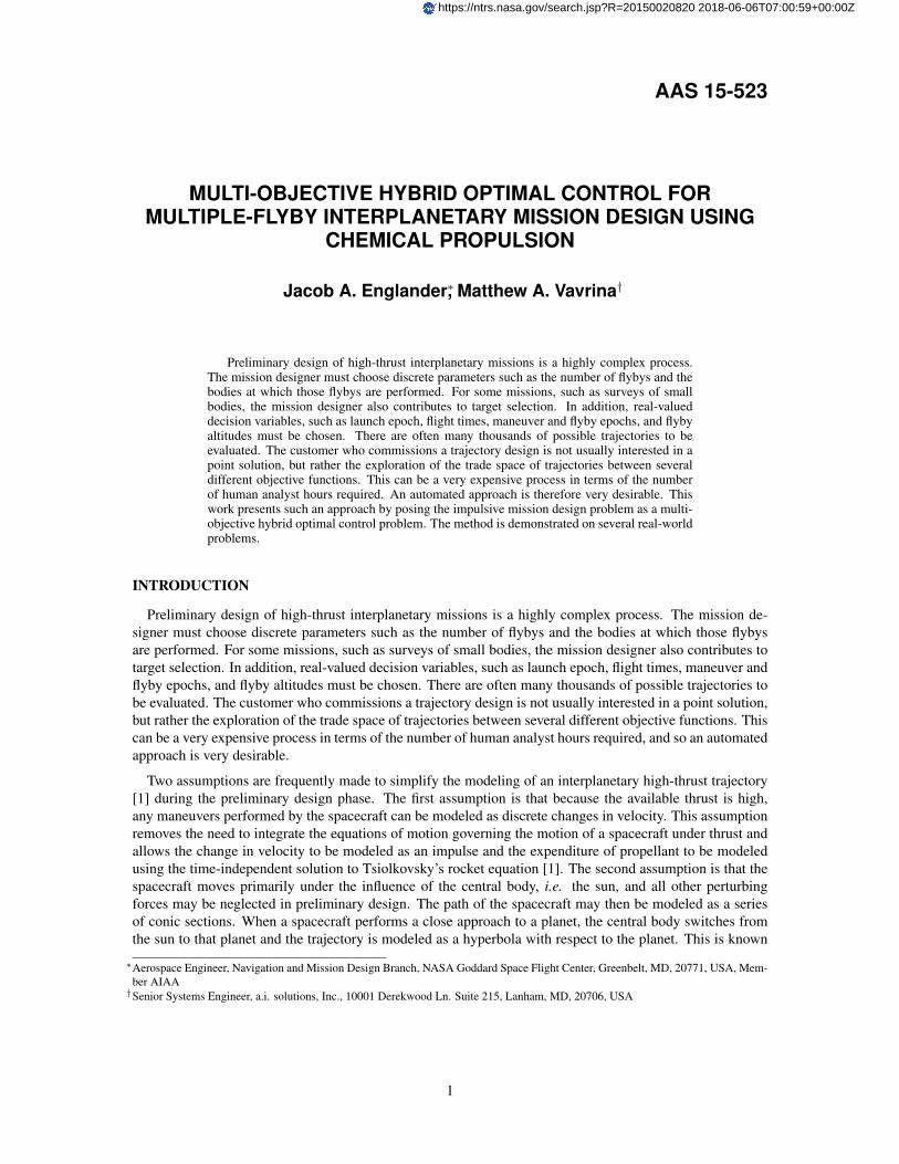
and then the flyby transfer angle δ, shown in Figure 2, may be found by

δ = 2 sin−1 (1/e) (7)

4

v∞−out

v∞−in

rp

δ

Figure 2: Definition of the flyby transfer angle δ

Finally, the incoming velocity vector must be rotated about the axis normal to the flyby hyperbola. Theoutgoing velocity vector is

v∞/out = v∞/in

(cos δi+ cos γ sin δj + sin γ sin δk

)(8)

where i, j, k are the unit vectors defining the b-plane:

i =v∞/in

v∞/in(9)

j =i× vpl∥∥∥i× vpl

∥∥∥ (10)

k = i× j (11)

The outgoing heliocentric velocity vector can then be found as

vsc/out = v∞/out + vbody (12)

As in the first phase of the mission, the spacecraft motion is then propagated in time by ηiti, after whichtime Lambert’s problem is solved again to find the arc and associated deep space maneuver necessary to bringthe spacecraft to the next planet in the sequence. If this planet is the last in the sequence, an intercept (flyby),rendezvous, or orbit insertion may be performed depending on the mission requirements.

The MGADSM problem may then be summarized as

Minimize f (x)where :

x =[tlaunch ∆vLV RLA DLA t1 ... tn−1 η1 ... ηn−1

Rp2 ... Rp(n−1) γ2 ... γn−1]

(13)

f (x) can be any relevant fitness function. A simple two-phase MGADSM mission is shown in Figure 3.

5

Figure 3: Diagram of a Two-Phase MGADSM Mission

Constraint Handling

A variety of constraints are considered in this work. There are two classes of constraints: constraints asso-ciated with feasibility of the trajectory model and constraints associated with the suitability of the trajectoryfor an actual mission.

The first feasibility constraint is on the energy of the spacecraft with respect to a flyby body at the momentof encounter, C3flyby, where

C3flyby = v2∞−in (14)

For sufficiently small values of C3flyby, Equation 6 yields an eccentricity very near zero even for an arbitrar-ily high periapse distance rp. Equation 7 then yields an arbitrarily large, non-physical turn angle. One way tothink of this conceptually is that for sufficiently small C3flyby, the encounter orbit is nearly parabolic and theapproximation of patching the heliocentric trajectory with a hyperbolic trajectory about the flyby body doesnot hold. It is possible to prevent this numerical singularity from affecting the trajectory design by imposinga nonlinear constraint on C3flyby, i.e.,

C3flyby ≥ C3min (15)

A value of C3min = 0.1 has been found empirically to work well.

The second model feasibility constraint deals with the well-known singularity in Lambert’s problem fortransfer angles of exactly 2π. This singularity, present in all solutions to Lambert’s problem, leads to unde-fined, non-physical behavior at that precise transfer angle. While very few final trajectory designs will sufferfrom this problem, the optimizer needs to be able to “walk” through the entire problem space on the way toan answer. Therefore it is necessary that the optimizer have some knowledge of the fact that the transfer angleis approaching 2π so that it can avoid the singularity. In this work, this is done with a nonlinear constraint.Noting that the transfer angle θLambert is given by,

θLambert = arccos

(r1 · r2

r1r2

)(16)

6

a transfer angle of 2π may be prevented by imposing a nonlinear constraint,

r1 · r2

r1r2≤ 1.0 (17)

Constraints 15 and 17 ensure that the trajectory represented by the MGADSM model always reflects reality.The trajectory designer may wish to impose additional constraints that deal with the suitability of a trajectorysolution for real-world use. Some of these constraints are straightforward, such as constraints on missionflight time, i.e.,

n∑i=1

ti ≤ tmax (18)

or an upper bound on terminal velocity at intercept, i.e.,

v∞−final ≤ vmax (19)

However, other constraints are more complex. Different types of missions impose different operationalconstraints. For example, there may be a constraint that the spacecraft must approach a small body on theilluminated side, i.e. the angle between the v∞ vector at arrival and the position vector of the body withrespect the sun must be less than some threshold angle θillumination, i.e.,

arccos

(v∞ · rbodyv∞rbody

)≤ θillumination (20)

Such a constraint can enable science operations or possibly be translated into financial terms by allowingthe spacecraft to fly with less capable sensors. This illumination constraint is just one of many possibleoperational constraints that could be imposed on a trajectory design problem. It is not sufficient to perform aglobal search on the unconstrained problem and then locally re-optimize on the constrained problem becausethe optimal solution to the constrained problem may not be in the neighborhood of the optimal solution tothe unconstrained problem. Similarly, it is not efficient to solve many permutations of the unconstrainedproblem and then filter away solutions that do not satisfy the constraints because then it is too easy to filteraway solutions that are almost feasible. Rather, it is better to include the operational constraints as part of theglobal search so that they can help shape the search process to be more efficient. This philosophy is followedin the second example presented in this work.

Objective Function, Launch Vehicle, and Ephemeris Modeling

Traditionally the objective function for a chemical mission is to minimize total ∆v. This is because ∆vcan be added linearly, whereas Tsiolkovsky’s rocket equation that governs spacecraft mass is exponential,i.e.,

mf = m0e−∆v/Ispg0 (21)

The linear quantity ∆v is easier for a gradient-based optimizer to handle because its derivatives with respectto the decision variables are well behaved, whereas the derivatives of Equation 21 are not. However Equation21 is not a completely accurate depiction of the cost of a mission because it does not take into account thatthe specific impulse (Isp) of the spacecraft thrusters and of the launch vehicle are different, and therefore thesame ∆v performed by the launch vehicle affects the spacecraft differently from what would happen if that∆v were performed by the spacecraft itself.

Classically the different performance of the spacecraft and launch vehicle is handled by tracking twoquantities, the ∆v performed by the spacecraft and the characteristic energy, or C3, of the launch. C3 isdefined as the square of the hyperbolic excess velocity of the spacecraft as it leaves the Earth. Many existingtools, such as STOUR [9], generate plots of C3 vs ∆v. An analyst can then pick a point from the plot andcompute the mass of the spacecraft as:

mf = m0 (C3) e−∆v/Ispg0 (22)

7

where m0 (C3) is the mass deliverable to a given C3 by the launch vehicle.

Plotting C3 vs ∆v works reasonably well in a combinatorial exploration of the mission design space butdoes not work as well in a numerical optimization method such as the one presented in this work, because itis undesirable to have two different objective functions. One can use a multi-objective inner-loop solver tofind the non-dominated front of C3 vs ∆v, but there is a better way. The key is in finding a single metricthat captures both C3 and ∆v and has well-behaved derivatives. Optimizing on mf directly accomplishesthis, but as noted above the derivatives with respect to the problem decision variables are not well behaved;Equation 22 is essentially an exponential decay with an enormous decay constant.

Fortunately taking a logarithm of Equation 22 makes the derivatives much more stable. In this work, theobjective function is:

J = − log 10 (mf ) = −log10(m0 (C3) e−∆v/Ispg0

)(23)

This choice of objective function is inspired by the original formulation of ∆v as a transformation of Equation21 but is more appropriate to a mission in which maneuvering is accomplished by two different propulsionsystems at different times as in Equation 22. The logarithm of 22 with respect to any base would probablywork well, log 10 is chosen for convenience and performs adequately.

Equation 23 requires a model of launch vehicle performance as a function of C3, which is provided as a5th degree polynomial:

mdelivered = (1− σLV )(aLV C

53 + bLV C

43 + cLV C

33 + dLV C

23 + eLV C3 + fLV

)(24)

where σLV is the user-defined launch vehicle margin in [0, 1] and the other coefficients are chosen by a curvefit to published launch vehicle performance data available at the Kennedy Space Center (KSC) expendablelaunch vehicle (ELV) performance website [28].

It is also necessary to provide accurate ephemeris modeling for all bodies used as destinations and/or flybytargets. Evolutionary Mission Trajectory Generator (EMTG) uses the SPICE toolkit [29] to provide thisinformation when possible, and when SPICE kernels are not available it uses static orbit elements.

Lower and Upper Bounds

EMTG’s stochastic optimizers require that the mission design problem be posed in a bounding box. If thebounds on the decision variables are too broad, the solvers will struggle to find a good solution. If the boundsare too negative than there is a risk of pruning away the optimal solution. Furthermore, because the trajectorydesign problem is being solved as the inner-loop of a HOCP, there is no opportunity for a human analyst tostep in and set appropriate bounds for every possible problem. Therefore a set of simple rules are used todetermine the bounds as shown in Table 1.

8

Table 1: Automated Choosing of Inner-Loop Bounds for MGADSM Problems

Parameter Lower Bound Upper BoundLaunch date user-defined user-definedStay time between journeys user-defined user-definedRLA 0.0 2πDLA user-defined user-definedv∞−launch 0.0 user-definedFor each phase:Flight time:(repeated flyby of same planet) T/2 (repeated flyby of same planet) 20T(outermost body has a < 2LU ) 0.1min (T1, T2) 2.0max (T1, T2)(outermost body has a ≥ 2LU ) max (T1, T2)Burn index η 0.01 0.99B-plane insertion angle γ −π πFlyby periapse distance ratio Rp 1.0 + hmax/Rbody 10 (rocky bodies)

300 (gas giants)

OUTER-LOOP OPTIMIZATION OF THE MISSION SEQUENCE

Outer-Loop Transcription

The mission design problem in this work is posed as two nested optimization problems, an “outer-loop”discrete optimization problem and an “inner-loop” real-valued optimization problem. The outer-loop solvesa multi-objective integer programming problem whose candidate solutions are themselves instances of theinner-loop trajectory optimization problem. The outer-loop works via a “cap and optimize” process by whichit chooses design variables such as destinations, flybys, and bounds on the launch date and flight time thatdefine a tractable inner-loop subproblem.

The user specifies a priori a list of outer-loop design variables and a “menu” of choices with correspondinginteger codes for each. In this work the design variables are launch epoch, time of flight, destinations, andflybys. The outer-loop algorithm makes one choice from each menu.

Launch epoch is transcribed as a menu of candidate launch dates plus a launch window size. For example,the user might specify launches in 2020, 2021, or 2022 with a 365 day launch window. The outer-loopchooses one of the available launch years and constructs an inner-loop problem where the spacecraft candepart Earth at any time during that year. The method for time of flight is similar - the user specifies a listof flight times and the optimizer chooses one and sets it as the upper-bound for the inner-loop problem. Nolower-bound is enforced - this seems to yield a more tractable inner-loop problem.

The user may also specify a menu of candidate destinations for each journey. For example, one mightwish to design a mission to two asteroids but have a long list of scientifically interesting options. The HOCPautomaton can choose the most accessible asteroids. The outer-loop may be instructed to discard candidatesolutions that visit the same destination body more than once.

Flyby sequence selection is similar to journey destination selection except that one does not always knowhow many flybys are to be performed. A “null-gene” technique is used to choose the number and identity offlyby bodies [17]. The analyst provides a list of acceptable flyby bodies and a maximum number of flybysfor each journey. Then, for each potential flyby, the outer-loop may select from a list containing the specifiedacceptable bodies and also a number of “null” options equal to the number of acceptable bodies. The outer-loop therefore has an equal probability of selecting “no flyby” for each opportunity as it does to select a flyby.This technique has been shown to be very effective for designing multi-flyby interplanetary missions andhas been used to reproduce the Cassini [17] trajectory and design an efficient variant of the BepiColombotrajectory [30].

9

Figure 4: Two-Dimensional, Non-Dominated Fronts of a Multi-Objective Trajectory Optimization Example

The user may then select any number of outer-loop objective functions for optimization. Some of these,such as flight time and launch year, may be directly related to decision variables. Others, such as final mass,may be the product of an the inner-loop optimization process. The inner-loop subproblem is optimized overonly one objective function but because the “cap and optimize” outer-loop constrains the inner-loop, eachsub-problem solution is a candidate solution to the multi-objective outer-loop problem.

Outer-Loop Multi-Objective Optimization via NSGA-II

The goal of multi-objective optimization is to generate the Pareto front of solutions [31]. The Pareto frontrepresents the set trade-off solutions in which no improvement can be achieved in one objective without de-grading at least one other objective. That is, all designs that compose the Pareto front are equally optimal. ThePareto front can be discontinuous and either concave or convex. Thus, the aim of multi-objective optimiza-tion is to generate numerous Pareto-optimal solutions such that a representation the Pareto front is created toenable a tradeoff decision. The Pareto front for a notional low-thrust trajectory optimization problem withthe objectives to maximize final spacecraft mass and minimize time of flight is illustrated in Figure 4. Themulti-objective optimization problem can be stated as:

minimize f (x)

subject to c (x) ≤ 0

xLB ≤ x ≤ xUB

(25)

where f (x) is a vector of objective functions, x is a vector of design variables, c (x) is a vector of constraintfunctions, and xLB and xUB are vectors of upper and lower bounds for x, respectively. The objective func-tions are often coupled, i.e. contain the same design variables, and also competing, i.e. the optimal solutionwith respect to one objective is not also the optimal solution with respect to the other objectives. Competitionbetween objectives creates the need to find multiple solutions, making multi-objective optimization morecomplex than single-objective optimization. The outer-loop of this work uses bounded but unconstrainedmulti-objective optimization, with the constraints c handled by the single-objective inner-loop.

The multi-objective optimization concept of domination allows for the comparison of a set of designswith multiple objectives, providing a measure of the relative quality of the design. When comparing twomulti-objective designs, the design x1 dominates design x2 if:

∀p : fp (x1) ≤ fp (x2) where p = 1, 2, ...nobjectives

∃p : fp (x1) < fp (x2)(26)

That is, x1 dominates design x2 if, for all objectives p, x1 is better than or equal to x2, and x1 outperformsx2 for at least one objective. In a direct comparison of two designs, if one design dominates another, that

10

design is closer in proximity to the Pareto front. If neither design dominates the other, the designs are non-dominant to each other. Therefore, in a set of designs, the superior designs are those that are not dominatedby any other design in the set, and are termed the non-dominated subset. It follows that any Pareto-optimaldesign is a member of the non-dominated subset associated with the entire feasible objective space and islocated along the Pareto front. A solution space with several Pareto fronts is shown in Figure 4.

A multi-objective genetic algorithm (MOGA) is an appropriate solution method for the outer-loop problem.A GA is a stochastic search and optimization technique that simulates natural selection and reproduction withthe goal of identifying globally-optimal designs. A GA first generates a random population of designs andthen iteratively executes three genetic operators: selection, crossover, and mutation. The operators are appliedto a parent population to produce a new offspring generation that is better adapted to fitness landscape definedby the objective functions. A GA does not require an initial guess or gradient information, making it ideal forexploring discrete, multi-modal, and expansive design spaces. A MOGA is a modified version of the standardGA that can solve multi-objective problems.

A MOGA is capable of finding the Pareto front for a multi-objective problem in a single optimizationrun. This is more efficient, in terms of computer time required, than performing many repetitions of asingle-objective optimization routine. One effective MOGA is the Non-Dominated Sorting Genetic Algo-rithm (NSGA) developed by Deb [32], in which the fitness of an individual in the population is based on itsrelative proximity to the population’s non-dominated front. The genetic operators of the NSGA evolve thepopulation toward the globally-optimal Pareto front in the same way that the population of a single-objectiveGA evolves toward the globally optimal solution.

A second generation non-dominated sorting genetic algorithm, the NSGA-II, improves upon the originalNSGA [25]. The NSGA-II incorporates mechanisms that ensure that the elite individuals, i.e. the bestindividuals in the population, are retained as the population evolves. Additionally, the NSGA-II employsstrategies that aim to produce a uniform representation of designs along the Pareto front. Domination isused to categorize each design into non-dominated fronts. The solutions composing the best non-dominatedfront are given a rank of one, and each subsequent front is given an incrementally higher rank according totheir relative distance to the Pareto front. The fast non-dominated sorting algorithm by Deb is outlined inAlgorithm 1, where m and n are individual solutions, Sm is the set of solutions that dominate m, cm is thenumber of solutions that dominate m, Fi are sets that contain the non-dominated fronts, Q is a temporary set,and nrank is rank of solution n.

The NSGA-II preserves diversity by preferring the solution that is in a less dense region of the objectivefunction space when comparing two solutions of the same rank. A crowding distance is assigned to eachindividual based on the perimeter of the hyper-rectangle formed with the two adjacent designs in objectivespace for each of each objective. The HOCP automaton described in this work employes a modified versionof Deb’s [25] crowding distance assignment to accommodate instances in which there are more than two ob-jectives and there are multiple solutions belonging to the same non-dominated front with the same minimumobjective function value. Whenever there are multiple solutions that take the minimum or maximum value fora given objective function coinciding in the same non-dominated front, the solutions with the lowest objectivefunction value for the other objectives are given a large crowding distance. The remaining solutions in theboundary group are assigned a crowding-distance based on a single adjacent solution for each objective. Thisapproach ensures that solutions with a minimum objective function value will not be discarded if the entirepopulation composes a single non-dominated front. The modified crowding distance assignment operator isdescribed in Algorithm 2, where I is the set of solutions to be sorted and the operator sort (I, p) refers tosorting a list I in ascending order by objective p. L is the set of solutions for a given objective p for which pis at a minimum and H is the set of solutions for which p is at a maximum, at the current generation.

After ranking the population using the non-dominated sort and crowding distance algorithms, NSGA-IIapplies genetic operators to the parent population to create an offspring population of the same size N . Theparent and offspring populations are then combined into a single population of size 2N . This combinedpopulation is then sorted and ranked according to non-domination. The next generation’s parent populationis created by taking each non-dominated front from the combined population, in rank order, until the new

11

Algorithm 1 Fast non-dominated sort [25]

for each individual m in population P doSm = ∅cm = 0for each individual n in population P do

if m dominates n thenSm = Sm

⋃n

else if n dominates m thencm = cm + 1

end ifend forif cm = 0 then

mrank = 1F1 = F1

⋃m

end ifend fori = 1while Fi 6= ∅ do

Q = ∅for each individual m in front Fi do

for each individual n in Sm docm = cm − 1if cm = 0 then

nrank = i+ 1Q = Q

⋃n

end ifend for

end fori = i+ 1Fi = Q

end while

parent population is filled. In this way the preservation of elite individuals is guaranteed and diversity inobjective space is promoted. The process is repeated for a set number of generations or length of time.

The NSGA-II is well-suited for the multi-objective trajectory optimization problem: it is capable of gener-ating the Pareto front to illustrate the trade-offs in the mission objectives of interest, can globally search thedesign, and is automated without requiring an initial guess.

Parallel Outer-Loop Optimization

The evaluation of the objective functions for a candidate solution is very expensive - it requires solving theentire inner-loop trajectory optimization problem and can take at best several seconds, in most cases manyminutes, and in some cases hours. Fortunately each inner-loop subproblem is independent of the others so it isnatural to evaluate them in parallel. The pool of N inner-loop subproblems to be evaluated is distributed overP processor cores. If N exceeds P, the subproblems are agglomerated into P task pools with one assigned toeach processor. The run-time is further decreased by saving each candidate solution to the outer-loop problemso that none must be evaluated more than once. Therefore the number of inner-loop instances to be run foreach outer-loop generation tends to decrease and the algorithm speeds up with each generation of NSGA-II.

There are two parallel processing paradigms: shared memory multiprocessing and distributed memorymulticomputing. Shared memory multiprocessing, also known as threading, is easier to implement but isnot appropriate for this work because it requires all processes to be “thread-safe,” i.e. do not interfere with

12

Algorithm 2 Modified Crowding-Distance Assignment

for each objective p doIp = sort (I, p)L = ∅H = ∅for i in Ip do

if p = 0 thenIp [i]distance = 0

end ifif fp (Ip [i]) = fmin

p thenA⋃B

L = L⋃Ip [i]

else if Ip [i]objective−value = fmaxp then

H =⋃H, Ip [i]

elseIp [i]distance = Ip [i]distance + (fp (Ip [i+ 1])− fp (Ip [i− 1])) /

(fmaxp − fmin

p

)end if

end forfor each objective q except p do

Lq = sort (L, q)Lq [0]distance =∞Hq = sort (L, q)Hq [0]distance =∞

end forend for

each other even while operating in the same memory space. However the SPICE ephemeris reader usedin this work is not thread-safe and therefore the entire algorithm cannot be used with shared memory mul-tiprocessing. Instead the algorithm described in this work is implemented using the distributed memorymulticomputing library message passing interface [33] in which each processor runs an independent processin distinct memory spaces.

INNER-LOOP TRAJECTORY OPTIMIZATION

Stochastic Global Search via Monotonic Basin Hopping and SNOPT

Because the solutions to the outer-loop problem require solutions to the inner-loop trajectory optimizationsubproblem, the performance of the HOCP automaton is only as good as the performance of the inner-loopsolver. A solver is required that can solve large, multi-modal problems with many nonlinear constraints.Because the inner-loop problem is generated in real time by the outer-loop, the inner-loop solver cannotrequire any human intervention and therefore cannot require an initial guess - a natural application for aheuristic stochastic search. The HOCP automaton described in this work uses monotonic basin hopping(MBH) [26, 34, 27, 7]. MBH, described in Algorithm 3, is a hybrid of a stochastic search step with annonlinear programming (NLP) solver. The stochastic search step efficiently explores the space and the NLPstep enforces the constraints and exploits local basins. The NLP step makes MBH particularly adept athandling challenging constraints such as the illumination angle constraint in Equation 20. The NLP step inthis work is performed using Sparse Nonlinear Optimizer (SNOPT) [35].

The MBH+NLP optimization algorithm in EMTG is efficient and does not require an initial guess. MBHis most useful when one does not have much a priori information about the solution as is always the casewhen solving an inner-loop trajectory optimization problem inside a hybrid optimal control (HOC) missiondesign problem.

13

Algorithm 3 Monotonic Basin Hopping (MBH)

generate random point xrun NLP solver to find point x∗ using initial guess xxcurrent = x∗

if x∗ is a feasible point thensave x∗ to archive

end ifwhile not hit stop criterion do

generate x′ by randomly perturbing xcurrent

for each time of flight variable ti in x′ doif rand (0, 1) < ρtime−hop then

shift ti forward or backward one synodic periodend if

end forrun NLP solver to find point x∗ from x′

if x∗ is feasible and f (x∗) < f (xcurrent) thenxcurrent = x∗

save x∗ to archiveelse if x∗ is infeasible and ‖c (x∗)‖ < ‖c (xcurrent)‖)

xcurrent = x∗

end ifend whilereturn best x∗ in archive

EXAMPLES

Jupiter Probe

In the first example, EMTG is used to design a notional mission to Jupiter in the 2020s. The spacecraft isto arrive at Jupiter and insert into an elliptical orbit with a semi-major axis of 140 RJ and an eccentricity of0.91. Some sequence of tour of Jupiter’s moons would then be conducted but is out of scope of this work,which focuses only on the interplanetary trajectory. The problem assumptions and solver settings for theJupiter example are shown in Table 2.

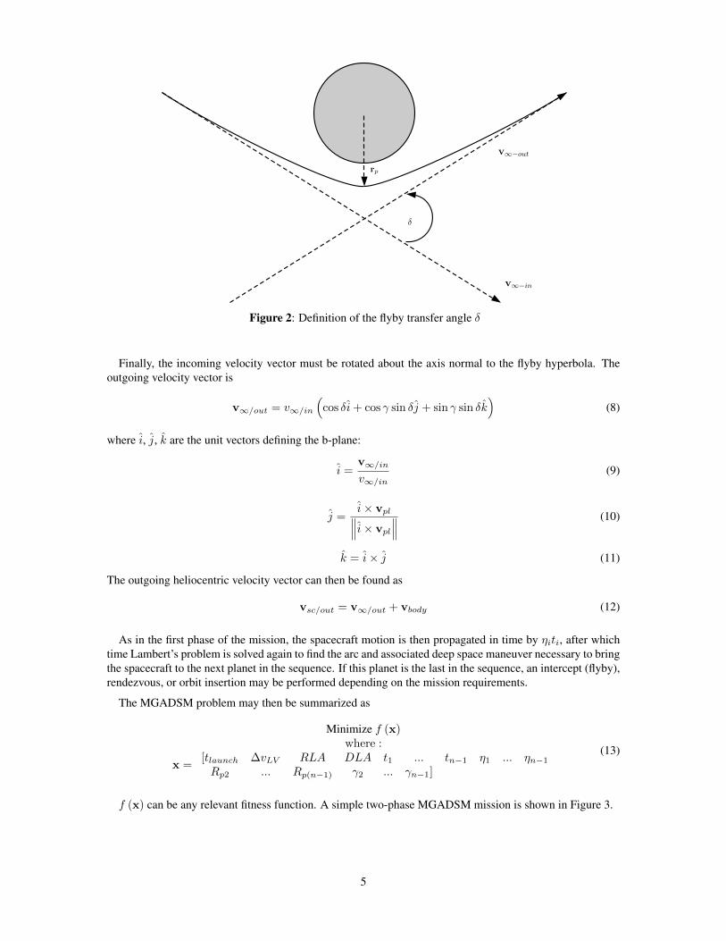
The outer-loop was run for 500 generations on a 64-core AMD Opteron running at 2.6 GHz, which tooktwo days and required no human interaction other than a few minutes to set up the initial problem. EMTGconsidered 8893 candidate outer-loop solutions, a non-dominated set of which are shown in Figure 5. Eachpoint in Figure 5 represents a completely different mission, including launch date, flight time, propulsivemaneuvers, and flybys. Two representative missions are shown in Figure 6. Figure ??(a) represents a missionwhich launches in 2021 but takes 8 years to deliver 2932 kg to Jupiter, while the mission in Figure ??(b)launches in 2026 and because of more favorable geometry delivers 3180 kg in only 5 years.

Whack-a-Rock

The second example presented here is a complex mission to deliver a high-velocity penetrator probe toa C-type near-Earth object (NEO) and then circle back around, rendezvous with the NEO, and inspect theimpact site in detail. This example is inspired by NASA’s Deep Impact mission, which delivered a penetratorprobe to comet Tempel 1 in 2005 [36]. One objective was to image the impact site but unfortunately so muchdust was thrown up that it could not be resolved. Unfortunately it was not possible to send Deep Impact backto Tempel 1 for a second look, so a second spacecraft, the re-purposed Stardust spacecraft was later sent toperform the observations [37]. In this example, hybrid optimal control is used to choose a target specificallyfor “re-accessibility.”

The set of allowable targets for the “Whack-a-Rock” mission is all NEOs of spectral type C and at least 500

14

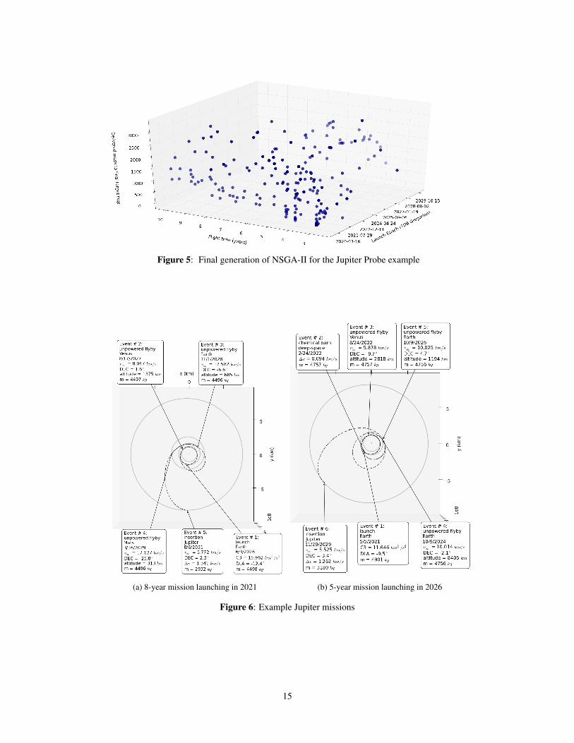
Figure 5: Final generation of NSGA-II for the Jupiter Probe example

(a) 8-year mission launching in 2021 (b) 5-year mission launching in 2026

Figure 6: Example Jupiter missions

15

Table 2: Assumptions and Settings for the Jupiter Probe Example

Description ValueLaunch year outer-loop chooses ∈ [2020, 2029]Flight time outer-loop chooses ∈ [3, 10] yearsLaunch vehicle Atlas V 551Spacecraft Isp 320 sArrival condition insert into orbit at Jupiter

a = 140RJ

e = 0.91Number of flybys allowed 5Flyby targets considered Venus, Earth, MarsOuter-loop objective functions launch year

flight timedelivered mass

Outer-loop population size 256Outer-loop mutation rate 0.3Inner-loop MBH run-time 10 minutesInner-loop MBH Pareto α 1.3

meters in diameter, as defined by the JPL small bodies database [38]. There are 25 targets in this list, as shownin Table 3. Whack-a-Rock is modeled in EMTG as a mission with two journeys, the first being from the Earthto the target and the second being to return to and rendezvous with the target. Up to two flybys of Venus,Earth, and/or Mars are allowed in each journey. The first journey ends in an intercept, i.e. a match of positionbut not velocity, with two constraints imposed. The first constraint is that the velocity magnitude at impactbe between 5 and 10 km/s. If the penetrator is too slow, it will not make an adequate crater. If it is too fast,its sampling instruments will not work. The second constraint is that the angle between the probe’s terminalvelocity and the target’s position with respect to the sun must be less than 70 as described in Equation 20.This ensures that the target is sufficiently illuminated for the penetrator’s terminal guidance system to work.Both of these constraints are incorporated into the inner-loop problem. The full set of problem assumptionsis shown in Table 4.

Once again EMTG was run for 350 generations on a 64-core AMD Opteron running at 2.6 GHz, witha total run time of about 3.8 days. EMTG evaluated 25141 candidate solutions, a non-dominated front ofwhich are shown in Figure 7. Each point in Figure 7 represents a different combination of target, flybys,launch vehicle, launch year, and flight time. The choice of launch vehicle is shown on the color axis, withredder being a larger launch vehicle.

Two of the many possible missions are shown in Figure 8. Both missions meet the Whack-a-Rock missionobjectives by delivering a probe with the required impact velocity and illumination angle and both delivermore than 2500 kg to rendezvous. However the two examples represent very different approaches to theproblem. One accomplishes the mission in a short time using the Atlas V 551 launch vehicle, and the otheraccepts a much longer flight time in exchange for the less expensive Atlas V 421. Depending on the needs ofthe customer, i.e. whether the cost of a larger launch vehicle is greater than or less than the cost of additionalflight time or alternatively depending on which candidate NEO is most scientifically attractive, any missionin Figure 7 could be chosen for detailed analysis and eventually flight.

CONCLUSION

Summary

In this work we show that the impulsive-thrust interplanetary mission design problem may be posed asa multi-objective HOCP and efficiently explored via the powerful combination of a multi-objective discrete

16

Table 3: Allowable targets for the “Whack-a-Rock” mission

Name a (AU) e i () Ω () ω ()2100 Ra-Shalom 0.83 0.44 15.76 170.84 356.043671 Dionysus 2.20 0.54 13.55 82.16 204.203691 Bede 1.77 0.28 20.36 348.77 234.8814402 1991DB 1.72 0.40 11.42 158.26 51.3215817 Lucianotesi 1.32 0.12 13.87 162.52 94.3016064 Davidharvey 2.85 0.59 4.54 335.61 104.8465706 1992NA 2.40 0.56 9.71 349.38 8.1085774 1998UT18 1.40 0.33 13.59 64.71 50.01136793 1997AQ18 1.15 0.47 17.38 296.30 36.98141079 2001XS30 1.16 0.83 28.53 251.47 0.87152563 1992BF 0.91 0.27 7.27 315.57 336.30152679 1998KU2 2.25 0.55 4.93 205.79 120.28162173 1999JU3 1.19 0.19 5.88 251.61 211.43162567 2000RW37 1.25 0.25 13.75 333.34 133.26175706 1996FG3 1.05 0.35 1.99 299.73 23.99308635 2005YU55 1.16 0.43 0.34 35.89 273.63322775 2001HA8 2.39 0.53 11.48 95.89 202.37370061 2000YO29 1.81 0.69 54.60 262.66 309.32413123 2001XS1 2.67 0.56 10.93 266.97 164.881997 AC11 0.91 0.37 31.64 116.94 141.621998 HT31 2.52 0.69 6.80 213.91 80.421999 VN6 1.73 0.37 19.48 58.10 43.562000 WL10 3.14 0.72 10.24 252.16 115.122001 SJ262 2.94 0.58 10.80 210.44 164.932002 DH2 2.05 0.54 20.94 345.56 231.79

Table 4: Assumptions and Settings for the Whack-a-Rock Example

Description ValueLaunch year outer-loop chooses ∈ [2020, 2029]Flight time outer-loop chooses ∈ [3, 12] yearsLaunch vehicle outer-loop chooses Atlas V 401, 411, 421, 431, 541, or 551Spacecraft Isp 320 sPenetrator mass 20 kgArrival conditions(first Journey) intercept with v∞ ∈ [5.0, 10.0] km/s, θillumination ≤ 70

(second Journey) rendezvousNumber of flybys allowed 2 in each JourneyFlyby targets considered Venus, Earth, MarsOuter-loop objective functions launch year

flight timedelivered masslaunch vehicle choice

Outer-loop population size 256Outer-loop mutation rate 0.3Inner-loop MBH run-time 10 minutesInner-loop MBH Pareto α 1.3

17

Figure 7: Final generation of NSGA-II for the Whack-a-Rock example

(a) 2501 kg delivered to 1999 JU3 on Atlas V 421 in11.25 years

(b) 2859 kg delivered to 1992 BF on Atlas V 551 in2.45 years

Figure 8: Example Whack-a-Rock missions

18

NSGA-II outer-loop with a MBH+NLP inner-loop. The trade space for a given mission and spacecraft designmay be characterized even when there is only enough time to evaluate a fraction of the full combinatorialdesign problem. The HOCP automaton presented here is shown very effective in exploring the design spacesfor a notional Jupiter probe and a very complex mission to impact and then revisit an NEO. Furthermorethe HOCP automaton is found to handle complex operational constraints such as the target illuminationconstraint.

The algorithm described here is in use at NASA Goddard Space Flight Center and offers three compellingadvantages. First, multiple mission cases may now be studied simultaneously, limited only by availablecomputing power. Second, mission design engineers can now spend more time with the customer and withspacecraft hardware engineers so that they can fully understand the scientific and engineering context of theirwork and deliver better value to the customer. Third, good mission ideas are much less likely to be rejecteddue to lack of time to work on mission design, and bad ideas are much more likely to be rejected beforethey consume too many resources because the full space of “what if” options may be explored autonomouslybefore a large team of specialists is brought to bear.

The algorithms described in this work are available as part of the open-source EMTG project [39]. Theauthors encourage the reader to examine and use them and welcome opportunities for collaboration withresearchers from all backgrounds.

ACKNOWLEDGMENTS

The authors would like to acknowledge Donald Ellison and Professor Bruce Conway at the Universityof Illinois for their ongoing contributions to the algorithms behind EMTG and hybrid optimal control ingeneral. The authors would also especially like to thank David Hinckley of the University of Vermont fordiscovering the need for a nonlinear constraint on Lambert transfer angle.. This research was funded by theNASA Goddard independent research and development program.

REFERENCES

[1] J. Prussing and B. Conway, Orbital Mechanics. Oxford University Press, New York, 1993.[2] M. Vasile and P. De Pascale, “Preliminary Design of Multiple Gravity-Assist Trajectories,” Journal of

Spacecraft and Rockets, Vol. 43, No. 4, 2006, pp. 794–805.[3] A. D. Olds, C. A. Kluever, and M. L. Cupples, “Interplanetary mission design using differential evolu-

tion,” Journal of Spacecraft and Rockets, Vol. 44, No. 5, 2007, pp. 1060–1070.[4] T. Vinko and D. Izzo, “Global Optimisation Heuristics and Test Problems for Preliminary Spacecraft

Trajectory Design,” Tech. Rep. GOHTPPSTD, European Space Agency, the Advanced Concepts Team,2008.

[5] M. Schlueter, J. Rckmann, and M. Gerdts, “Non-linear mixed-integer-based Optimisation Technique forSpace Applications,” Poster for ESA NPI Day, 2010.

[6] M. Vasile, E. Minisci, and M. Locatelli, “Analysis of some global optimization algorithms for spacetrajectory design,” Journal of Spacecraft and Rockets, Vol. 47, No. 2, 2010, pp. 334–344.

[7] J. A. Englander and A. C. Englander, “Tuning Monotonic Basin Hopping: Improving the Efficiency ofStochastic Search as Applied to Low-Thrust Trajectory Optimization,” 24th International Symposiumon Space Flight Dynamics, Laurel, MD, May 2014.

[8] B. Barbee, P. Abell, D. Adamo, C. Alberding, D. Mazanek, L. Johnson, D. Yeomans, C. P. W., A. Cham-berlin, and V. Friedensen, “The Near-Earth Object Human Space Flight Accessible Targets Study: AnOngoing Effort to Identify Near-Earth Asteroid Destinations for Human Explorers,” 2013 IAA PlanetaryDefense Conference, April 2013.

[9] J. Longuski and S. Williams, “Automated design of gravity-assist trajectories to Mars and the outerplanets,” Celestial Mechanics and Dynamical Astronomy, Vol. 52, No. 3, 1991, pp. 207–220.

[10] J. Downing, “Pyxis Tool,” Tech. Rep. NASA/TM-2006-214139, Flight Dynamics Branch (FDAB),NASA Goddard Space Flight Center, August 2006.

[11] A. Gad and O. Abdelkhalik, “Hidden Genes Genetic Algorithm for Multi-Gravity-Assist TrajectoriesOptimization,” Journal of Spacecraft and Rockets, Vol. 48, July-August 2011, pp. 629–641.

[12] O. Abdelkhalik and A. Gad, “Dynamic-Size Multi-Population Genetic Optimization for Multi-Gravity-Assist Trajectories,” Journal of Guidance, Control, and Dynamics, Vol. 35, March-April 2012,p. 520529.

19

[13] M. Vasile and S. Campagnola, “Design of low-thrust multi-gravity assist trajectories to Europa,” Journalof the British Interplanetary Society, Vol. 62, No. 1, 2009, pp. 15–31.

[14] M. Buss, M. Glocker, M. Hardt, O. v. Stryk, R. Bulirsch, and G. Schmidt, “Nonlinear Hybrid DynamicalSystems: Modeling, Optimal Control, and Applications,” Lecture Notes in Control and InformationSciences, Vol. 279, 2002, pp. 311–335.

[15] I. M. Ross and C. D’Souza, “Hybrid Optimal Control Framework for Mission Planning,” Journal ofGuidance, Control, and Dynamics, Vol. 28, July-August 2005, pp. 686–697.

[16] B. Conway, C. Chilan, and B. Wall, “Evolutionary principles applied to mission planning problems,”Celestial Mechanics and Dynamical Astronomy, Vol. 97, No. 2, 2007, pp. 73 – 86.

[17] J. Englander, B. Conway, and T. Williams, “Automated Mission Planning via Evolutionary Algorithms,”Journal of Guidance, Control, and Dynamics, Vol. 35, No. 6, 2012, pp. 1878–1887.

[18] J. A. Englander, Automated Trajectory Planning for Multiple-Flyby Interplanetary Missions. PhD the-sis, University of Illinois at Urbana-Champaign, April 2013.

[19] V. Coverstone-Carroll, J. Hartmann, and W. Mason, “Optimal multi-objective low-thrust spacecraft tra-jectories,” Computer Methods in Applied Mechanics and Engineering, Vol. 186, No. 24, 2000, pp. 387– 402.

[20] M. Vavrina and K. Howell, “Multiobjective Optimization of Low-Thrust Trajectories Using a GeneticAlgorithm Hybrid,” AAS/AIAA Space Flight Mechanics Meeting, February 2009. AAS 09-141.

[21] M. Vasile and F. Zuiani, “MACS: A hybrid multiobjective optimization algorithm applied to space tra-jectory optimization, Journal of Aerospace Engineering,” Proceedings of the Institution of MechanicalEngineers Part G, Vol. 225, 2011, pp. 1211–1227.

[22] D. Izzo, D. Hennes, and A. Riccardi, “Constraint Handling and Multi-Objective Methods for the Evo-lution of Interplanetary Trajectories,” AIAA Journal of Guidance, Control, and Dynamics, Vol. 4, 2014,pp. 792–799.

[23] J. Englander, M. Vavrina, and A. Ghosh, “Multi-Objective Hybrid Optimal Control for Multiple-FlybyLow-Thrust Mission Design,” AAS/AIAA Space Flight Mechanics Meeting, January 2015.

[24] M. Vavrina, J. Englander, and A. Ghosh, “Coupled Low-Thrust Trajectory and Systems OptimizationVia Multi-objective Hybrid Optimal Control,” AAS/AIAA Space Flight Mechanics Meeting, January2015. AAS 15-397.

[25] K. Deb, S. Agrawal, A. Pratap, , and T. Meyarivan, “A fast and elitist multi-objective genetic algorithm:NSGA-II,” IEEE Transactions on Evolutionary Computation, Vol. 6, April 2002, pp. 182–197.

[26] R. Leary, “Global optimization on funneling landscapes,” Journal of Global Optimization, Vol. 18,December 2000, pp. 367–383.

[27] A. Cassioli, D. Izzo, D. Di Lorenzo, M. Locatelli, and F. Schoen, “Global Optimization Approaches forOptimal Trajectory Planning,” Modeling and Optimization in Space Engineering (G. Fasano and J. D.Pintr, eds.), Vol. 73 of Springer Optimization and Its Applications, pp. 111–140, Springer New York,2013.

[28] “NASA Launch Services Program Performance Web Site,” October 2014.[29] “SPICE Ephemeris,” August 2013. http://naif.jpl.nasa.gov/naif/.[30] J. A. Englander, B. A. Conway, and T. Williams, “Automated Interplanetary Mission Planning,”

AAS/AIAA Astrodynamics Specialist Conference, Minneapolis, MN, August 2012.[31] V. Pareto, Manuale di Economica Politica. Milano, Italy: Societa Editrice Libraria, 1906. translated

into English by A. Schwier as Manual of Political Economy, MacMillan Press, New York, 1971.[32] C. A. Coello, G. B. Lamont, and D. A. Veldhuizen, Evolutionary Algorithms for Solving Multi-Objective

Problems (Genetic and Evolutionary Computation), 2nd ed. Springer-Verlag, 2006.[33] “MPI: A Message-Passing Interface Standard,” tech. rep., Message Passing Forum, Knoxville, TN,

USA, 1994.[34] C. Yam, D. d. Lorenzo, and D. Izzo, “Low-Thrust Trajectory Design as a Constrained Global Optimiza-

tion Problem,” Proceedings of the Institution of Mechanical Engineers, Part G: Journal of AerospaceEngineering, Vol. 225, 2011, pp. 1243–1251.

[35] P. E. Gill, W. Murray, and M. A. Saunders, “SNOPT: An SQP Algorithm for Large-Scale ConstrainedOptimization,” SIAM Rev., Vol. 47, No. 1, 2005, pp. 99–131.

[36] “Deep Impact: Your First Look Inside a Comet!,” http://deepimpact.umd.edu/.[37] “Stardust-NExT,” http://stardustnext.jpl.nasa.gov/.[38] “JPL Small-Body Database Search Engine,” June 1 2015.[39] “EMTG (Evolutionary Mission Trajectory Generator),” https://sourceforge.net/

projects/emtg/.

20