aaron cook thesis - montana.edu
TRANSCRIPT
CHARACTERIZATION OF INTERLAMINAR FRACTURE IN COMPOSITE
MATERIALS
A CASE STUDY APPROACH
by
Aaron Michael Cook
A thesis submitted in partial fulfillmentof the requirements for the degree
of
Master of Science
in
Mechanical Engineering
MONTANA STATE UNIVERSITY-BOZEMANBozeman, Montana
July 2001

ii
APPROVAL
of a thesis submitted by
Aaron Michael Cook
This thesis has been read by each member of the thesis committee and has beenfound to be satisfactory regarding content, English usage, format, citations, bibliographicstyle, and consistency, and is ready for submission to the College of Graduate Studies.
Dr. Douglas Cairns________________________________________ __________(Signature) Date
Approved for the Department of Mechanical & Industrial Engineering
Dr. Vic Cundy________________________________________ __________(Signature) Date
Approved for the College of Graduate Studies
Dr. Bruce McLeod________________________________________ __________ (Signature) Date

iii
STATEMENT OF PERMISSION TO USE
In presenting this thesis in partial fulfillment of the requirements for a master's
degree at Montana State University-Bozeman, I agree that the Library shall make it
available to borrowers under rules of the Library.
If I have indicated my intention to copyright this thesis by including a copyright notice
page, copying is allowable only for scholarly purposes, consistent with "fair use" as
prescribed in the U.S. Copyright Law. Requests for permission for extended quotation
from or reproduction of this thesis in whole or in parts may be granted only by the
copyright holder.
Signature ______________________________
Date __________________________________

iv
ACKNOWLEDGMENTS
I thank Dr. Douglas Cairns and Dr. John Mandell for their assistance and motivation in
this research. I would also like to thank Dr. Ladean McKittrick for serving as a graduate
committee member, and for providing guidance in the field of finite element analysis.
Additional gratitude is offered to the sponsors involved in this study. Pratt & Whitney,
AlliantechSystems, Advanced Composite Group, and the D.O.E. EPSCOR all provided
funding and unique research opportunities. A special thanks is also extended to the
members of the Composite Technology Research Team. Daniel Samborsky was
especially helpful with his knowledge and suggestions for experimental testing. I am
additionally thankful to Dr. Cundy and the Industrial and Mechanical Engineering
Department’s administrative team.
v
TABLE OF CONTENTS
LIST OF FIGURES ..........................................................................................................xi
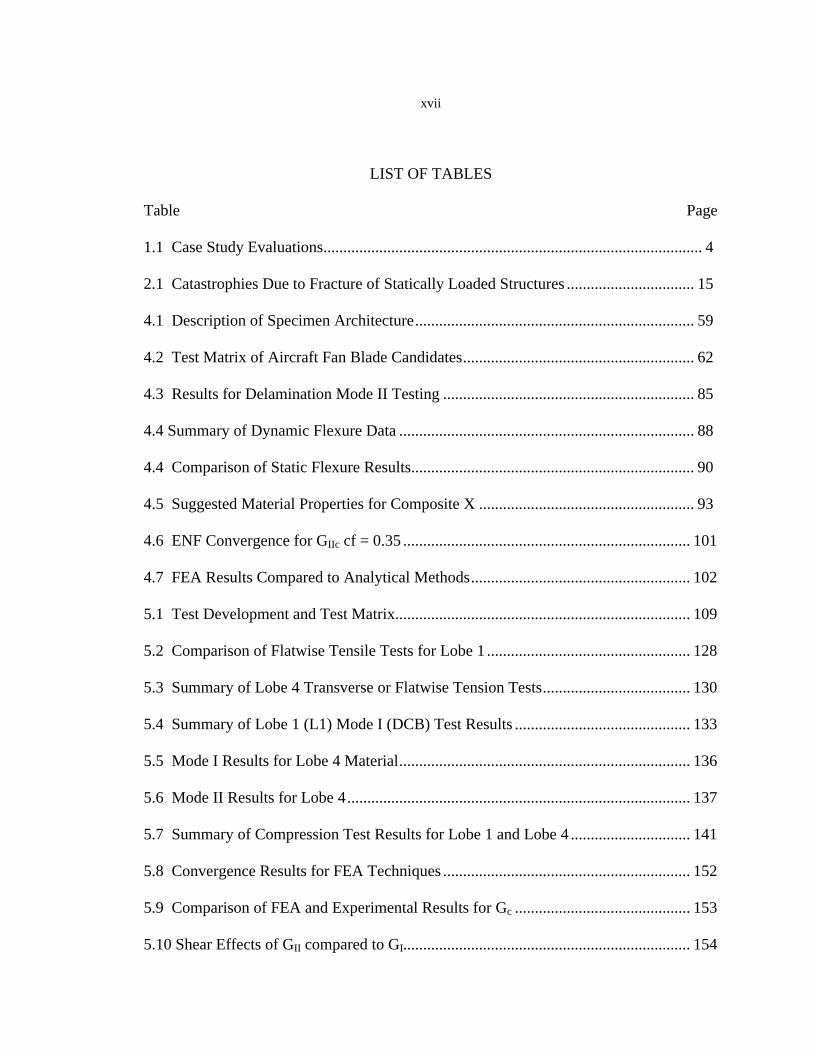
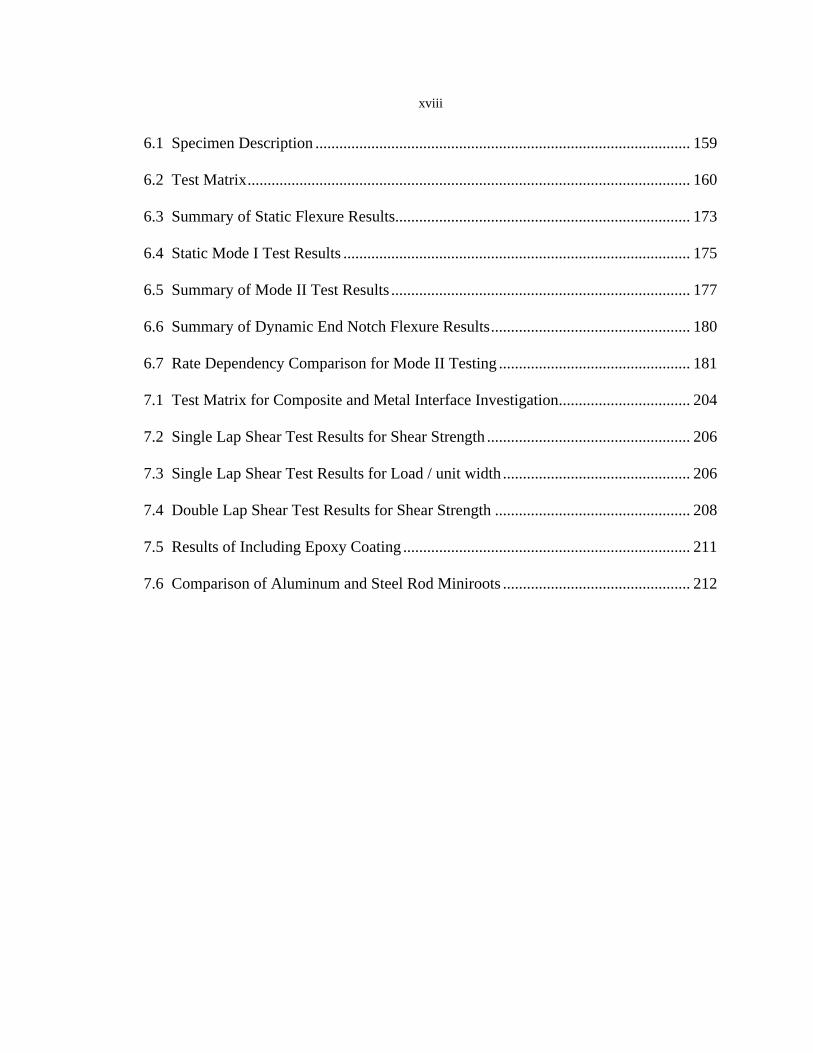
LIST OF TABLES......................................................................................................... xvii
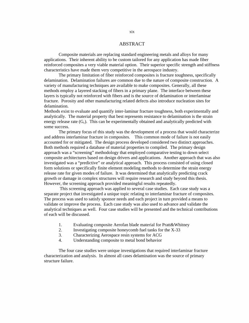
ABSTRACT ................................................................................................................. xix
1. INTRODUCTION ........................................................................................................ 1
Composite Materials ..................................................................................................... 1Needs............................................................................................................................. 2Available Technology ................................................................................................... 2Goals ............................................................................................................................. 3Case Study Approach.................................................................................................... 3Case I Carbon Fiber Aerofan Blades ............................................................................ 5Case II Honeycomb Sandwich Fuel Tanks ................................................................... 6Case III Low Temperature Cure Composite Structures................................................ 7Case IV Composite to Metal Interfaces ........................................................................ 8Evaluation Methodology............................................................................................... 9
2. BACKGROUND ........................................................................................................ 10
Composites ................................................................................................................. 10Advantages and Disadvantages............................................................................ 10In-plane and Out of Plane Properties ................................................................... 11Manufacturing ..................................................................................................... 12
Failure Types and Related Theories ........................................................................... 12Strength of Materials Approach........................................................................... 13Fracture Mechanics Approach Background and History..................................... 14
Interlaminar Fracture .................................................................................................. 15Fracture Mechanics Overview.................................................................................... 16
Mode I .................................................................................................................. 17Testing Procedure for DCB Specimen................................................................. 19Data Reduction Methods ......................................................................................21Mode II................................................................................................................. 22Testing Procedure for ENF Specimen ................................................................. 23Data Reduction Methods...................................................................................... 26
Finite Element Theory................................................................................................ 27Benefits ................................................................................................................ 27Models and Modeling Procedure ......................................................................... 28Step1 Geometry Development............................................................................ .29Step 2 Element Choice......................................................................................... 29Step 3 Constitutive Properties.............................................................................. 31
vi
Step 4 Meshing .................................................................................................... 31Step 5 and 6 Application of Constraints and Loads............................................. 32Step 7 and 8 Solution and Results ....................................................................... 32
Finite Element as Related to Fracture Mechanics ...................................................... 32Strain Energy Release Rate Methods................................................................... 33Virtual Crack Closure Techniques....................................................................... 33Crack Extension Techniques................................................................................ 36
3. INTERLAMINAR FRACTURE CHARACTERIZATION PROCESS.................... 38
Needs.......................................................................................................................... 38Optimization .............................................................................................................. 39Fracture Toughness Tips and Tradeoffs .................................................................... 39
Resin System........................................................................................................ 40Fibers.................................................................................................................... 40Inhomogeneities................................................................................................... 41Porosity ................................................................................................................ 41Ply-drops and Dissimilar Material Interface........................................................ 42Interlaminar Zone and Other Inhomogeneities .................................................... 43
Prediction and Screening Approach........................................................................... 44Database............................................................................................................... 45Screening Process ................................................................................................ 46Screening Procedure ............................................................................................ 47Prediction Approach ............................................................................................ 49
Composite Design...................................................................................................... 51
4. CASE STUDY I COMPOSITE AEROFAN BLADE EVALUATION..................... 54
Project Introduction.................................................................................................... 54Existing Work ...................................................................................................... 55Full Scale testing and Need for Screening Process.............................................. 56Problem Statement ............................................................................................... 57Design Drivers and Material Limitations ............................................................ 58Materials Provided and Specimen Description.................................................... 58Material Property Isolation .................................................................................. 60Test Matrix........................................................................................................... 61
Experimental Procedures............................................................................................ 63Basic In-plane and Interlaminar Properties.......................................................... 63Delamination Mode II Testing............................................................................. 63Apparatus ............................................................................................................. 64Procedure ............................................................................................................. 66Data Reduction..................................................................................................... 68Dynamic Flexure Testing..................................................................................... 74Apparatus ............................................................................................................. 75
vii
Procedure ............................................................................................................. 75Data Reduction..................................................................................................... 75Static Flexure Testing .......................................................................................... 78Apparatus ............................................................................................................. 78Procedure ............................................................................................................. 79Data Reduction..................................................................................................... 80Tensile Test.......................................................................................................... 81Apparatus ............................................................................................................. 81Procedure ............................................................................................................. 81
Experimental Results.................................................................................................. 83Mode II Delamination Resistance Results........................................................... 83Dynamic Flexure Results..................................................................................... 86Static Flexure Results .......................................................................................... 89Tensile Test Results ............................................................................................. 91Summary of Experimental Results ...................................................................... 92
Numerical Analysis for Case Study I ......................................................................... 94Static Flexure Approach ...................................................................................... 94Static Flexure Model............................................................................................ 94Static Flexure Numerical Results......................................................................... 96End Notch Flexure Approach .............................................................................. 98End Notch Flexure Model.................................................................................... 99End Notch Flexure Results ................................................................................ 101Comparison ........................................................................................................ 102Test Specimen Validation .................................................................................. 104
Summary for Case Study I ....................................................................................... 105
5. CASE STUDY II HONEYCOMB FUEL TANK INVESTIGATION..................... 108
Project Introduction.................................................................................................. 108Case Study Goal................................................................................................. 109
Experimental Procedures.......................................................................................... 110Flatwise Tension Testing ................................................................................... 111Specimen Preparation ........................................................................................ 113Testing Procedure .............................................................................................. 114Data Reduction Methods.................................................................................... 115Mode I Testing................................................................................................... 118Testing Procedure .............................................................................................. 119Data Reduction Methods.................................................................................... 119Mode II Testing.................................................................................................. 121Testing Procedure .............................................................................................. 122Data Reduction Methods.................................................................................... 122Flatwise Compression Testing........................................................................... 125Specimen Preparation ........................................................................................ 125Testing Procedure .............................................................................................. 125
viii
Data Reduction Methods.................................................................................... 126Experimental Results................................................................................................ 127
Flatwise Tension Results ................................................................................... 128Discussion of Flatwise Tension Results ............................................................ 130Mode I Results ................................................................................................... 131Mode II Results.................................................................................................. 137Discussion of Mode II Results........................................................................... 138Flatwise Compression Results ........................................................................... 140Discussion of Flatwise Compression Results .................................................... 140
Numerical Analysis of Honeycomb Fuel Tank Investigation .................................. 142Motivation.......................................................................................................... 142Flatwise Tension ................................................................................................ 142Approach............................................................................................................ 143Model ................................................................................................................. 143Results................................................................................................................ 144Solution and Mesh Convergence ....................................................................... 145Mode I ................................................................................................................ 149Approach............................................................................................................ 149Model ................................................................................................................. 150Solution and Convergence ................................................................................. 151Comparison ........................................................................................................ 152Mode II............................................................................................................... 154
Summary for Case Study II ...................................................................................... 155Epilogue ............................................................................................................. 156
6. CASE STUDY III AEROSPACE RESIN EVALUATION ..................................... 157
Project Introduction.................................................................................................. 157Problem Statement ............................................................................................. 158Material and Specimen Description................................................................... 159Test Matrix......................................................................................................... 160
Experimental Methods ............................................................................................. 161Static Flexure ..................................................................................................... 161Static Flexure Apparatus.................................................................................... 161Static Flexure Testing Procedure ....................................................................... 162Static Flexure Data Reduction ........................................................................... 163Fracture Toughness Testing............................................................................... 163DCB Testing Procedure ..................................................................................... 163DCB Data Reduction Methods .......................................................................... 165Mode II............................................................................................................... 165ENF Testing Procedure...................................................................................... 165ENF Data Reduction Methods ........................................................................... 166Dynamic Mode II Testing.................................................................................. 167Dynamic ENF Apparatus................................................................................... 167
ix
Dynamic ENF Testing Procedure ...................................................................... 167Dynamic ENF Data Reduction .......................................................................... 168Scanning Electron Microscopy Evaluations ...................................................... 171SEM Apparatus.................................................................................................. 171SEM Testing Procedure ..................................................................................... 171
Experimental Results................................................................................................ 173Static Flexure Test Results................................................................................. 173Mode I Results from DCB Testing .................................................................... 174Mode II Results from Static ENF Testing ......................................................... 177Mode II Results from Dynamic ENF Testing.................................................... 179SEM Results for Selected Systems .................................................................... 182
Summary for Case Study III..................................................................................... 186
7. CASE STUDY IV METAL INTERFACE............................................................... 188
Bond Characteristics................................................................................................. 188Chemical Bond................................................................................................... 189Structural Interlock ............................................................................................ 189Need for Simpler Structure and Methodology................................................... 189Lap Shear ........................................................................................................... 190
Single Lap Shear ...................................................................................................... 190Shear Lap Construction...................................................................................... 191Shear Lap Configuration.................................................................................... 191Test Procedure ................................................................................................... 192Data Reduction................................................................................................... 192
Double Lap Shear ..................................................................................................... 193Double Lap Shear Configuration ....................................................................... 193Double Lap Shear Construction......................................................................... 194Double Lap Shear Test Procedure and Data Reduction..................................... 194
Miniroot.................................................................................................................... 195Miniroot Construction........................................................................................ 195Miniroot Configuration...................................................................................... 196Testing Procedure .............................................................................................. 197Data Reduction................................................................................................... 198Sample Results................................................................................................... 198Debonding.......................................................................................................... 199
Metal Interface Experimental Results ...................................................................... 200Parametric Study................................................................................................ 200Surface Treatment.............................................................................................. 201Elastic Properties ............................................................................................... 201Chemical Bond Characteristics.......................................................................... 201Mechanical Bond Characteristics ...................................................................... 202Knurling ............................................................................................................. 202
x
Threading ........................................................................................................... 202Resin Systems .................................................................................................... 202Layup Variations................................................................................................ 203Insert Material .................................................................................................... 203Insert Coating..................................................................................................... 203Test Matrix......................................................................................................... 204Single Lap Shear Results ................................................................................... 205Double Lap Shear Results.................................................................................. 207Miniroot Experimental Results .......................................................................... 209Insert Coating Effects ........................................................................................ 209Geometry Effects ............................................................................................... 211Mechanical Interlock ......................................................................................... 213
Metal Interface Numerical Study ............................................................................ 214SLS Motivation and Approach .......................................................................... 214Model ................................................................................................................. 215Results................................................................................................................ 216Miniroot Motivation and Approach ................................................................... 218Model ................................................................................................................. 218Results................................................................................................................ 219
Summary for Case Study IV .................................................................................... 221
8. CONCLUSIONS AND FUTURE WORK ............................................................... 223
Composite Material Design Process......................................................................... 224Importance of the Screening Process ....................................................................... 225Case Study Review................................................................................................... 225
Case Study I Composite Aerofan Blade Evaluation .......................................... 226Case Study II X-33 Fuel Tank Investigation ..................................................... 227Case Study III Aerospace Composite Resin Characterization........................... 228Case Study IV Metal Interface Evaluation ........................................................ 228
Future Recommendations......................................................................................... 229
REFERENCES CITED.................................................................................................. 230
APPENDIX A: FINITE ELEMENT CODES .............................................................. 235
xi
LIST OF FIGURES
Figure Page
1.1 PW-4000-112 Aerofan Blade ..................................................................................... 5
1.2 Honeycomb Fuel Cell ................................................................................................. 6
1.3 Composite Applications for Resins Evaluated ........................................................... 7
1.4 Composite Wind Turbine............................................................................................ 8
2.1 Fiber and Transverse Directions of a Composite...................................................... 11
2.2 Laminate Construction.............................................................................................. 12
2.3 Three Modes of Fracture and Related Loading ........................................................ 17
2.4 DCB Test in Progress................................................................................................ 18
2.5 DCB Testing Geometry ............................................................................................ 19
2.6 Mode I Fracture Propagation Behavior of a Composite Specimen .......................... 20
2.7 ENF Test in Progress ................................................................................................ 23
2.8 Mode II Fracture Specimen Geometry...................................................................... 24
2.9 Typical Mode II Crack Behavior .............................................................................. 25
2.10 Mode II Crack Behavior with Hysteresis Captured................................................ 25
2.11 VCCT-1 Schematic with 8 Node Quadrilateral Elements ...................................... 34
2.12 VCCT-2 Schematic for Mode I Closure ................................................................. 35
3.1 Porosity in a Composite Laminate............................................................................ 41
3.2 Sandwich Panel Material with Ply Drops .................................................................. 42
3.3 Resin Rich Region in a Laminated Composite .......................................................... 43
3.4 Database Construction Process .................................................................................. 46
xii
3.5 Screening Approach................................................................................................... 48
3.6 Analytical Process for Fracture Modeling ................................................................. 50
4.1 Example of Impact and Dynamic Flex Testing Rectangular Specimen ................... 60
4.2 Impact Testing Fixture.............................................................................................. 64
4.3 Data Acquisition Used for Experimental Testing..................................................... 65
4.4 Force vs. Time Output for Series 5 Laminate........................................................... 67
4.5 Acceleration vs. Time for 5 Series Laminate............................................................ 69
4.6 Velocity Profile for 5 Series Laminate ..................................................................... .70
4.7 Displacement vs. Time for 5 Series Laminate .......................................................... 72
4.8 Dynamic Load vs. Displacement Trace for Series 5 Laminate ................................ 73
4.9 Dynamic Flexure Behavior…................................................................................... 76
4.10 Static Flexure Test Fixture and Specimen .............................................................. 78
4.11 Static Flexure Behavior........................................................................................... 79
4.12 Tensile Test Behavior ............................................................................................. 82
4.13 Delamination Results for 5 Series Material ............................................................ 84
4.14 Force vs. Time for Dynamic Flexure Tests ............................................................ 86
4.15 Force vs. Deflection for Dynamic Flexure Tests .................................................... 87
4.16 Static Flexure Comparison...................................................................................... 89
4.17 Tensile Test Results ................................................................................................ 91
4.18 Stress vs. Strain for 5 Series ................................................................................... 92
4.19 FEA Static Flexure Model ...................................................................................... 95
4.20 Comparison of Experimental Static Flexure Results to Numerical ........................ 96
4.21 Longitudinal Stress Plot from FEA Solution ......................................................... 97
xiii
4.22 ENF Mesh with Refined Region and Boundary Conditions................................ 100
4.23 Friction Effects on Predicted Mode II Fracture Toughness................................. 103
5.1 Sampling of Panel 1 From Lobe 1 .......................................................................... 110
5.2 Sampling of Panel 2 From Lobe 4 .......................................................................... 111
5.3 Mounting (Glue) Fixture Used to Attach Tabs to Specimen .................................. 112
5.4 Flatwise Tension Specimen Complete with Attached Tabs ................................... 114
5.5 Testing Jig with Universal Pivoting Capability (flexible coupler) ......................... 115
5.6 Graphical Presentation of Flatwise Tension Specimen .......................................... 117
5.7a Mode I Testing Apparatus...................................................................................... 118
5.7b Test in Progress...................................................................................................... 118
5.8 Three Successive Loading Cases for Lobe 4 Material............................................ 120
5.9 Mode II Testing Apparatus In Progress .................................................................. 121
5.10 Mode II Test Results of Lobe 4 Material.............................................................. 123
5.11 Mode II Test Showing Constant Loading During Crack Growth......................... 124
5.12 Compression Testing Configuration ..................................................................... 126
5.13 Typical Compression Test Result for Lobe 4 ....................................................... 127
5.14 Graphical Behavior of Lobe 4 Material in Flatwise Tension ............................... 129
5.15 Comparison of Failure Modes of Lobe 4 to Lobe 1.............................................. 129
5.16 Peel-off Test Results for Lobe 1 Material L1-DCB-4 .......................................... 131
5.17 Lobe 1 Material Specimen Core Shear Failure..................................................... 134
5.18 Failure Mode of Lobe 4 Material.......................................................................... 135
5.19 Comparison of Static Flexure and ENF Results for Lobe 4 ................................. 139
xiv
5.20 FWT Flatwise (Transverse) Tension Model ......................................................... 144
5.21 FWT Stress Distribution with Core Close-up....................................................... 145
5.22 FWT Solution Convergence ................................................................................. 146
5.23 Plane Stress vs. Plane Strain ................................................................................. 147
5.24 Stress Profile Based on Offset Distance ............................................................... 148
5.25 Stress Profile without Singularities....................................................................... 148
5.26 DCB Model for Sandwich Material ...................................................................... 151
6.1 Static Flexure Test Results for 6867 Material ........................................................ 162
6.2 Hysteretic Behavior of 6866 DCB – 3 Specimen ................................................... 164
6.3 Mode II Crack Behavior with Hysteresis Captured................................................ 166
6.4 Force vs. Time Data for 6868 XHTM Material ...................................................... 168
6.5 Acceleration vs. Time for 6868 XHTM Material ................................................... 169
6.6 Velocity Profile for 6868 XHTM Material ............................................................. 169
6.7 Displacement vs. Time for 6868 XHTM Material.................................................. 170
6.8 Dynamic Load vs. Displacement Curve for 6868 XHTM Material ....................... 170
6.9 SEM Photo.............................................................................................................. 172
6.10 Mode I Results for Varying Post Cure Temperatures........................................... 176
6.11 Mode II Fracture Toughness as a Function of Postcure Temperature .................. 179
6.12A 6863 npc at 1500 ................................................................................................ 183
6.12B 6863 npc at 500 .................................................................................................. 183
6.12C 6863 pc177 at 1500 ............................................................................................ 183
6.12D 6863 pc177 at 500 .............................................................................................. 183
xv
6.13A 6865 npc at 1500 ................................................................................................ 184
6.13B 6865 npc at 500 .................................................................................................. 184
6.13C 6865 pc177 at 1500 ............................................................................................ 184
6.13D 6865 pc177 at 500 .............................................................................................. 184
6.14A 6866 npc at 1500 ................................................................................................ 185
6.14B 6866 npc at 500 .................................................................................................. 185
6.14C 6866 pc177 at 1500 ............................................................................................ 185
6.14D 6866 pc177 at 500 .............................................................................................. 185
7.1 Fatigue Specimen, R112 Cross-Section ................................................................. 188
7.2 Single Lap Shear Specimen .................................................................................... 191
7.3 Double Lap Shear Specimen (DLS) ....................................................................... 194
7.4 Array of Miniroot Variations .................................................................................. 196
7.5 Miniroot Anatomy .................................................................................................. 197
7.6 Lap Shear and Miniroot Test Approach.................................................................. 198
7.7 Miniroot Failure Characteristics ............................................................................. 199
7.8 Effects of Using Epoxy Coating as an Intermediate Adhesive............................... 210
7.9 Debond Behavior of Miniroots with Round Inserts................................................ 212
7.10 Failure of 45 Degree Diamond Knurled Steel Insert Miniroot ............................. 213
7.11 Shear Stress Singularity Effects............................................................................ 215
7.12 SLS FEA Model and Mesh Detail ........................................................................ 216
7.13 Lap Shear Analytical and Numerical Results for Etched Vinylester.................... 217
7.14 Miniroot FEA Shear Stress Plot for Vinylester .................................................... 219

xvi
7.15 Shear Stress Data From Peak to Level Stress ....................................................... 220
xvii
LIST OF TABLES
Table Page
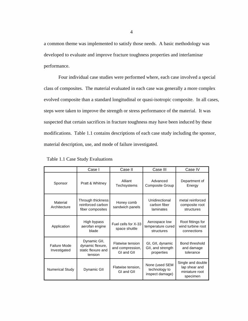
1.1 Case Study Evaluations............................................................................................... 4
2.1 Catastrophies Due to Fracture of Statically Loaded Structures ................................ 15
4.1 Description of Specimen Architecture...................................................................... 59
4.2 Test Matrix of Aircraft Fan Blade Candidates.......................................................... 62
4.3 Results for Delamination Mode II Testing ............................................................... 85
4.4 Summary of Dynamic Flexure Data .......................................................................... 88
4.4 Comparison of Static Flexure Results....................................................................... 90
4.5 Suggested Material Properties for Composite X ...................................................... 93
4.6 ENF Convergence for GIIc cf = 0.35 ........................................................................ 101
4.7 FEA Results Compared to Analytical Methods....................................................... 102
5.1 Test Development and Test Matrix.......................................................................... 109
5.2 Comparison of Flatwise Tensile Tests for Lobe 1 ................................................... 128
5.3 Summary of Lobe 4 Transverse or Flatwise Tension Tests..................................... 130
5.4 Summary of Lobe 1 (L1) Mode I (DCB) Test Results ............................................ 133
5.5 Mode I Results for Lobe 4 Material......................................................................... 136
5.6 Mode II Results for Lobe 4...................................................................................... 137
5.7 Summary of Compression Test Results for Lobe 1 and Lobe 4 .............................. 141
5.8 Convergence Results for FEA Techniques .............................................................. 152
5.9 Comparison of FEA and Experimental Results for Gc ............................................ 153
5.10 Shear Effects of GII compared to GI........................................................................ 154
xviii
6.1 Specimen Description .............................................................................................. 159
6.2 Test Matrix............................................................................................................... 160
6.3 Summary of Static Flexure Results.......................................................................... 173
6.4 Static Mode I Test Results ....................................................................................... 175
6.5 Summary of Mode II Test Results ........................................................................... 177
6.6 Summary of Dynamic End Notch Flexure Results.................................................. 180
6.7 Rate Dependency Comparison for Mode II Testing ................................................ 181
7.1 Test Matrix for Composite and Metal Interface Investigation................................. 204
7.2 Single Lap Shear Test Results for Shear Strength ................................................... 206
7.3 Single Lap Shear Test Results for Load / unit width ............................................... 206
7.4 Double Lap Shear Test Results for Shear Strength ................................................. 208
7.5 Results of Including Epoxy Coating ........................................................................ 211
7.6 Comparison of Aluminum and Steel Rod Miniroots ............................................... 212
xix
ABSTRACT
Composite materials are replacing standard engineering metals and alloys for manyapplications. Their inherent ability to be custom tailored for any application has made fiberreinforced composites a very viable material option. Their superior specific strength and stiffnesscharacteristics have made them very competitive in the aerospace industry.
The primary limitation of fiber reinforced composites is fracture toughness, specificallydelamination. Delamination failures are common due to the nature of composite construction. Avariety of manufacturing techniques are available to make composites. Generally, all thesemethods employ a layered stacking of fibers in a primary plane. The interface between theselayers is typically not reinforced with fibers and is the source of delamination or interlaminarfracture. Porosity and other manufacturing related defects also introduce nucleation sites fordelamination.Methods exist to evaluate and quantify inter-laminar fracture toughness, both experimentally andanalytically. The material property that best represents resistance to delamination is the strainenergy release rate (Gc). This can be experimentally obtained and analytically predicted withsome success.
The primary focus of this study was the development of a process that would characterizeand address interlaminar fracture in composites. This common mode of failure is not easilyaccounted for or mitigated. The design process developed considered two distinct approaches.Both methods required a database of material properties to compiled. The primary designapproach was a “screening” methodology that employed comparative testing to down selectcomposite architectures based on design drivers and applications. Another approach that was alsoinvestigated was a “predictive” or analytical approach. This process consisted of using closedform solutions or specifically finite element modeling methods to determine the strain energyrelease rate for given modes of failure. It was determined that analytically predicting crackgrowth or damage in complex structures will require research and study beyond this thesis.However, the screening approach provided meaningful results repeatedly.
This screening approach was applied to several case studies. Each case study was aseparate project that investigated a unique topic relating to interlaminar fracture of composites.The process was used to satisfy sponsor needs and each project in turn provided a means tovalidate or improve the process. Each case study was also used to advance and validate theanalytical techniques as well. Four case studies will be presented and the technical contributionsof each will be discussed.
1. Evaluating composite Aerofan blade material for Pratt&Whitney2. Investigating composite honeycomb fuel tanks for the X-333. Characterizing Aerospace resin systems for ACG4. Understanding composite to metal bond behavior
The four case studies were unique investigations that required interlaminar fracturecharacterization and analysis. In almost all cases delamination was the source of primarystructure failure.

1
CHAPTER 1
INTRODUCTION
This focus of this study is on the delamination and interlaminar fracture
performance of composite materials. General testing methods and procedures were
employed to evaluate the fracture performance of sponsor supplied materials.
Additionally, various methods of analysis were used for fracture toughness evaluation,
including FEA (finite element analysis). Guidelines were generated for improving design
with regard to fracture toughness. A general methodology for the characterization of
composite laminates was developed employing standard procedures and analysis
techniques.
Composite Materials
Fiber reinforced composite materials are replacing standard isotropic materials in
many applications. Aerospace vehicles, aircraft, marine equipment, and common items
such as civil structures, prosthetic devices, and sports equipment are currently being
constructed of such composite materials.
The primary advantage of composite materials is their inherent ability to be
custom tailored to a specific design situation. Constituents like fibers and matrix material
can be used in different combinations, amounts, and architectures to obtain an optimal
material composition.
A major drawback to laminated composite materials stems from the
manufacturing process used to construct them. Placing fabric or fibers in strata to obtain
2
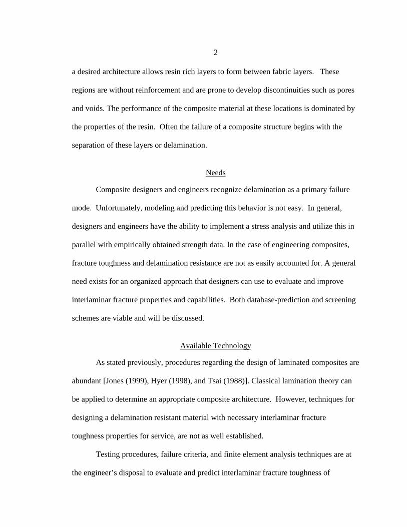
a desired architecture allows resin rich layers to form between fabric layers. These
regions are without reinforcement and are prone to develop discontinuities such as pores
and voids. The performance of the composite material at these locations is dominated by
the properties of the resin. Often the failure of a composite structure begins with the
separation of these layers or delamination.
Needs
Composite designers and engineers recognize delamination as a primary failure
mode. Unfortunately, modeling and predicting this behavior is not easy. In general,
designers and engineers have the ability to implement a stress analysis and utilize this in
parallel with empirically obtained strength data. In the case of engineering composites,
fracture toughness and delamination resistance are not as easily accounted for. A general
need exists for an organized approach that designers can use to evaluate and improve
interlaminar fracture properties and capabilities. Both database-prediction and screening
schemes are viable and will be discussed.
Available Technology
As stated previously, procedures regarding the design of laminated composites are
abundant [Jones (1999), Hyer (1998), and Tsai (1988)]. Classical lamination theory can
be applied to determine an appropriate composite architecture. However, techniques for
designing a delamination resistant material with necessary interlaminar fracture
toughness properties for service, are not as well established.
Testing procedures, failure criteria, and finite element analysis techniques are at
the engineer’s disposal to evaluate and predict interlaminar fracture toughness of

3
composite materials. These available technologies can be combined and expressed in
terms of a general methodology for fracture performance evaluation. In turn, this
methodology can be employed to enhance the performance of composite structures.
Montana State University’s Composite Technology Team has routinely
investigated delamination type failures [Orozco (1999)]. Standard test procedures have
been applied to unidirectional laminated composites to evaluate and quantify fracture
toughness. These procedures have been focused at the evaluation of resin performance in
composite architectures. Significant effort has been directed at applying finite element
analysis and fracture techniques to the evaluation of these baseline composites. Studies
have also been extended towards applying these procedures to more complex structures,
such as T-sections [Haugen (1998) and Morehead (2000)].
Goals
Ultimately the procedures and techniques used to quantify the fracture toughness
performance of composite specimens can be used to predict failure of more complex
composite structures. The goal of the current study is to provide a systematic engineering
approach to help develop laminated architectures, evaluate interlaminar fracture
properties, and improve performance of engineering composites in commercial
applications.
Case Study Approach
Several investigations were conducted to address both the strength and fracture
toughness characteristics of different composite candidates. Each project possessed
individual specific needs imposed by the demands of the commercial sponsor. However,
4
a common theme was implemented to satisfy those needs. A basic methodology was
developed to evaluate and improve fracture toughness properties and interlaminar
performance.
Four individual case studies were performed where, each case involved a special
class of composites. The material evaluated in each case was generally a more complex
evolved composite than a standard longitudinal or quasi-isotropic composite. In all cases,
steps were taken to improve the strength or stress performance of the material. It was
suspected that certain sacrifices in fracture toughness may have been induced by these
modifications. Table 1.1 contains descriptions of each case study including the sponsor,
material description, use, and mode of failure investigated.
Case I Case II Case III Case IV
Sponsor Pratt & WhitneyAlliant
TechsystemsAdvanced
Composite GroupDepartment of
Energy
Material Architecture
Through thickness reinforced carbon fiber composites
Honey comb sandwich panels
Unidirectional carbon fiber laminates
metal reinforced composite root
structures
ApplicationHigh bypass
aerofan engine blade
Fuel cells for X-33 space shuttle
Aerospace low temperature cured
structures
Root fittings for wind turbine root
connections
Failure Mode Investigated
Dynamic GII, dynamic flexure, static flexure and
tension
Flatwise tension and compression,
GI and GII
GI, GII, dynamic GII, and strength
properties
Bond threshold and damage
tolerance
Numerical Study Dynamic GIIFlatwise tension,
GI and GII
None (used SEM technology to
inspect damage)
Single and double lap shear and miniature root
specimen
Table 1.1 Case Study Evaluations
5
Each of the case studies focuses on a specific aspect of delamination or
interlaminar fracture. The materials in these studies were evaluated for advanced
aerospace applications.
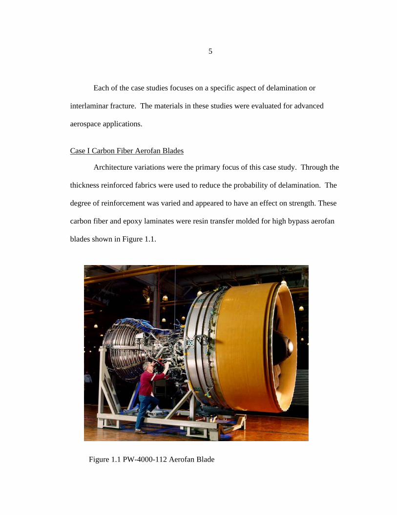
Case I Carbon Fiber Aerofan Blades
Architecture variations were the primary focus of this case study. Through the
thickness reinforced fabrics were used to reduce the probability of delamination. The
degree of reinforcement was varied and appeared to have an effect on strength. These
carbon fiber and epoxy laminates were resin transfer molded for high bypass aerofan
blades shown in Figure 1.1.
Figure 1.1 PW-4000-112 Aerofan Blade
6
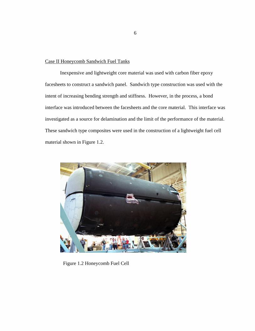
Case II Honeycomb Sandwich Fuel Tanks
Inexpensive and lightweight core material was used with carbon fiber epoxy
facesheets to construct a sandwich panel. Sandwich type construction was used with the
intent of increasing bending strength and stiffness. However, in the process, a bond
interface was introduced between the facesheets and the core material. This interface was
investigated as a source for delamination and the limit of the performance of the material.
These sandwich type composites were used in the construction of a lightweight fuel cell
material shown in Figure 1.2.
Figure 1.2 Honeycomb Fuel Cell
7
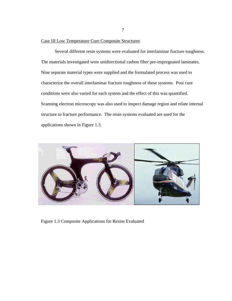
Case III Low Temperature Cure Composite Structures
Several different resin systems were evaluated for interlaminar fracture toughness.
The materials investigated were unidirectional carbon fiber pre-impregnated laminates.
Nine separate material types were supplied and the formulated process was used to
characterize the overall interlaminar fracture toughness of these systems. Post cure
conditions were also varied for each system and the effect of this was quantified.
Scanning electron microscopy was also used to inspect damage region and relate internal
structure to fracture performance. The resin systems evaluated are used for the
applications shown in Figure 1.3.
Figure 1.3 Composite Applications for Resins Evaluated

8
Case IV Composite to Metal Interfaces
In general, information regarding the bond characteristics between metal and
composites is limited. The interface between the metal and composite or resin was
identified as a potential delamination site. Experimental test methods were developed
and implemented. FEA was also used to validate and interpret experimental findings.
The metal inserts were in use for the root connections of a composite wind turbine blade
in this case (shown in Figure 1.4). They were molded into a composite laminate and used
for bolted connections to a hub.
Figure 1.4 Composite Wind Turbine

9
Evaluation Methodology
A general methodology was developed that, employs predictive techniques and
screening processes to evaluate a materials fracture toughness performance. The
experimental methods used are presented, as well as analytical techniques. The process
and related technology were then applied to the three case studies described above. Some
of the results are specific to the sponsor and their specific demands. However, the
approach was generalized and can be applied to other similar design situations.
10
CHAPTER 2
BACKGROUND
Composites
The first person to construct a home from mud and straw may have been the first
composite designer. However, many people attribute the space race and its demand for
higher flying, faster, and lighter aircraft to be the largest source of growth and
development in composite materials [Hyer (1998)]. Aerospace applications have
provided knowledge and technology that have spread to commonalities such as sports
equipment and simple civilian structures.
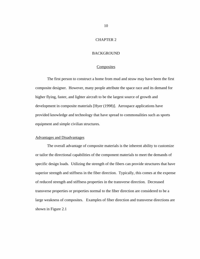
Advantages and Disadvantages
The overall advantage of composite materials is the inherent ability to customize
or tailor the directional capabilities of the component materials to meet the demands of
specific design loads. Utilizing the strength of the fibers can provide structures that have
superior strength and stiffness in the fiber direction. Typically, this comes at the expense
of reduced strength and stiffness properties in the transverse direction. Decreased
transverse properties or properties normal to the fiber direction are considered to be a
large weakness of composites. Examples of fiber direction and transverse directions are
shown in Figure 2.1
11
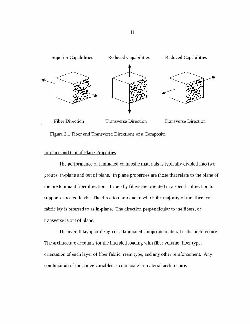
In-plane and Out of Plane Properties
The performance of laminated composite materials is typically divided into two
groups, in-plane and out of plane. In plane properties are those that relate to the plane of
the predominant fiber direction. Typically fibers are oriented in a specific direction to
support expected loads. The direction or plane in which the majority of the fibers or
fabric lay is referred to as in-plane. The direction perpendicular to the fibers, or
transverse is out of plane.
The overall layup or design of a laminated composite material is the architecture.
The architecture accounts for the intended loading with fiber volume, fiber type,
orientation of each layer of fiber fabric, resin type, and any other reinforcement. Any
combination of the above variables is composite or material architecture.
Superior Capabilities Reduced Capabilities Reduced Capabilities
Fiber Direction Transverse DirectionTransverse Direction
Figure 2.1 Fiber and Transverse Directions of a Composite
12
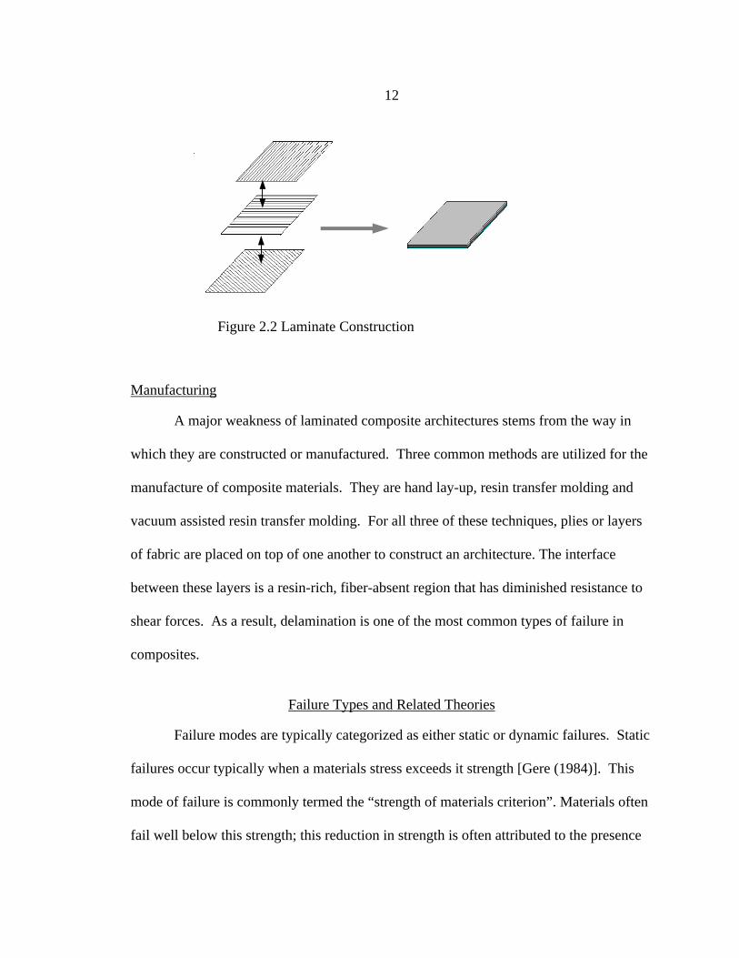
Manufacturing
A major weakness of laminated composite architectures stems from the way in
which they are constructed or manufactured. Three common methods are utilized for the
manufacture of composite materials. They are hand lay-up, resin transfer molding and
vacuum assisted resin transfer molding. For all three of these techniques, plies or layers
of fabric are placed on top of one another to construct an architecture. The interface
between these layers is a resin-rich, fiber-absent region that has diminished resistance to
shear forces. As a result, delamination is one of the most common types of failure in
composites.
Failure Types and Related Theories
Failure modes are typically categorized as either static or dynamic failures. Static
failures occur typically when a materials stress exceeds it strength [Gere (1984)]. This
mode of failure is commonly termed the “strength of materials criterion”. Materials often
fail well below this strength; this reduction in strength is often attributed to the presence
Figure 2.2 Laminate Construction
13
of cracks and flaws. When the stress intensity at a crack front exceeds the material’s
critical stress intensity factor, failure occurs. Accounting for or predicting this type of
failure is the science of fracture mechanics. Examples of dynamic or time dependent
failures are creep and fatigue. These types of failures and analysis will not be addressed
in this study.
Strength of Materials Approach
Static stress failure criteria exist for both ductile and brittle materials. Typically a
maximum combined stress state is analyzed and compared to the material’s strength
[Norton (1996)]. The material’s design strength is usually based on a published value or
a quantity obtained empirically. A variety of experimental methods are available for
determining material strength and depend mostly on material type. Ductile materials,
such as steel and aluminum, are traditionally evaluated with the maximum distortion
energy criterion, often referred to as the Henky-von-Mises Criterion. Brittle materials are
not accurately represented by this criterion. As a result, the Coulomb Mohr theory is
usually preferred for evaluating and assessing limiting stresses of brittle materials such as
cast iron [Norton (1996)]. Composite material strengths are not accurately represented
by either of the above failure criterion, primarily due to their anisotropic nature.
Although composite materials are not usually classified as ductile materials and
are not isotropic, often the maximum stress or a modification of the von-Mises criterion
is employed to estimate the failure stress [Norton (1996)]. This method can be accurate
depending on the application, but not for general cases. An improved criterion for
evaluating limiting stresses for composites is the Tsia-Wu criterion [Hyer (1998), Jones

14
(1999) and Tsai (1971)]. This method accounts for the anisotropic construction and
behavior of composites. The Tsia-Wu criterion offers a unique advantage. This method
can be used to analyze each layer or laminae of the structure individually. Then, the
limiting layer of entire architecture is isolated, and the corresponding limiting stress is
found. An overview summarizing and comparing these criteria can be found in Tsai
(1971).
Fracture Mechanics Approach Background and History
The strength of materials approach to static failure assumes a material to be
homogenous in some cases, isotropic in some cases, and free of defects such as micro-
cracks and voids in all cases. These assumptions are not always valid. With the case of
metals and alloys, cracks are typically caused by manufacturing and processing
treatments. Small cracks are almost always present and should be accounted for in
analysis. Components can fail at stresses well below the material’s strength when cracks
are present. When the critical amount of energy is present or when the stress intensity is
adequate, crack propagation occurs. Brittle type fracture in ductile materials has been the
cause of many catastrophic disasters [Broek (1996) and ASM (1997)]. A brief timeline
of noteworthy fracture induced failures is offered below in Table 2.1.

15
The failures in Table 2.1 are all fracture failures of metal structures. The stress-
state during the catastrophe was below the critical strength of the structure’s material.
The cause of failure in each of these events is commonly believed to be the result of
brittle fracture. Interestingly enough, steel is known to exhibit a ductile to brittle
transition in behavior at low temperatures. Most of the above failures occurred during
winter or colder months.
Interlaminar Fracture
Metals are not the only materials susceptible to failure due to fracture or crack
propagation. Composite materials are often vulnerable to fracture type failure called
interlaminar fracture. Interlaminar fracture occurs when the plies or layers separate.
Often voids, pores, or other small defects are present between layers. These
Table 2.1 Catastrophies Due to Fracture of Statically Loaded Structures
Date Event
March 19th 1830Montrose Suspension bridge
chains gave way during a boat race resulting in many deaths
1860-1870200 deathes/year due to wheel and axle fractures in England
January 19th 1919Boston Molasses Tank Rupture
killed 21 people
January 16th 1943WWII tankers cracked in half due to residual stresses and cracking
from welding.

16
discontinuities provide nucleation or initiation points for separation to occur.
Interlaminar fracture is a common mode of failure for composite materials, especially in
laminated architectures [Hyer (1998), Broek (1996), and Jones (1999)]. This failure
phenomenon will be a focus of this study.
Fracture Mechanics Overview
As stated previously, failure can occur in a material or structure at stresses well
below the yield or ultimate strength. Griffith stated that “crack propagation will occur if
the energy released upon crack growth is sufficient to provide all the energy that is
required for crack growth [Griffith (1920)].” Griffith’s criterion can be mathematically
expressed as:
where U is the elastic energy,
W is the energy required for crack growth,
a is the crack length and (da) is the change in crack length.
G is the strain energy release rate or crack driving force and is equal to (dU/da).
The energy consumed in crack propagation is denoted by R=dW/da, which is
called the crack resistance [Broek (1996)].
There are three distinct modes of fracture that are related directly to the manner of
loading. These modes are denoted as mode I, mode II, and mode III type fractures. All
three modes are shown in Figure 2.3, as well as the loading required to induce them.
da
dW
da
dU≥ (2.1)
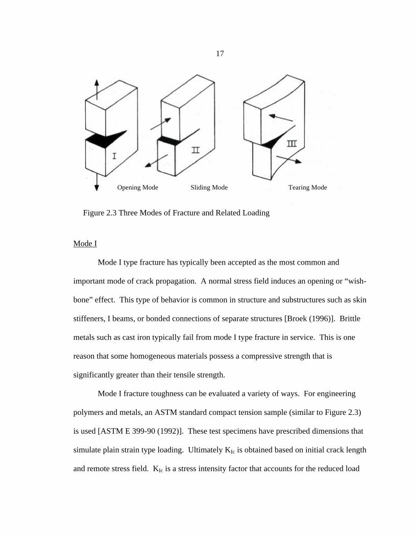
17
Mode I
Mode I type fracture has typically been accepted as the most common and
important mode of crack propagation. A normal stress field induces an opening or “wish-
bone” effect. This type of behavior is common in structure and substructures such as skin
stiffeners, I beams, or bonded connections of separate structures [Broek (1996)]. Brittle
metals such as cast iron typically fail from mode I type fracture in service. This is one
reason that some homogeneous materials possess a compressive strength that is
significantly greater than their tensile strength.
Mode I fracture toughness can be evaluated a variety of ways. For engineering
polymers and metals, an ASTM standard compact tension sample (similar to Figure 2.3)
is used [ASTM E 399-90 (1992)]. These test specimens have prescribed dimensions that
simulate plain strain type loading. Ultimately KIc is obtained based on initial crack length
and remote stress field. KIc is a stress intensity factor that accounts for the reduced load
Opening Mode Sliding Mode Tearing Mode
Figure 2.3 Three Modes of Fracture and Related Loading
18
handling capability of a material based on stress concentrations from cracks. Some
iterations may be necessary to provide valid test results. This type of testing is usually
only valid for high strength-brittle materials and homogenous materials in general.
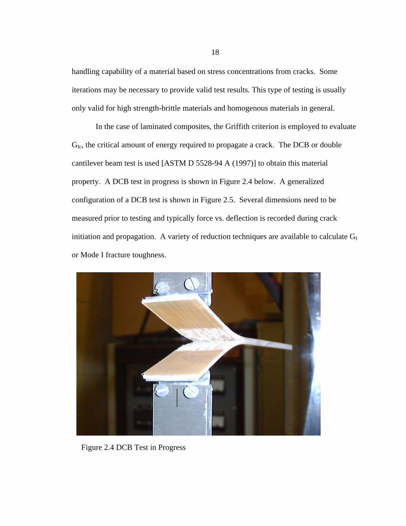
In the case of laminated composites, the Griffith criterion is employed to evaluate
GIc, the critical amount of energy required to propagate a crack. The DCB or double
cantilever beam test is used [ASTM D 5528-94 A (1997)] to obtain this material
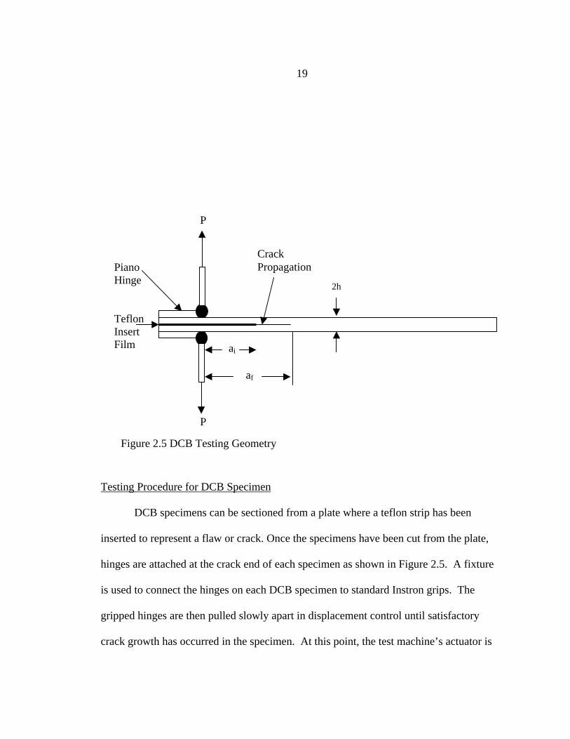
property. A DCB test in progress is shown in Figure 2.4 below. A generalized
configuration of a DCB test is shown in Figure 2.5. Several dimensions need to be
measured prior to testing and typically force vs. deflection is recorded during crack
initiation and propagation. A variety of reduction techniques are available to calculate GI
or Mode I fracture toughness.
Figure 2.4 DCB Test in Progress
19
Testing Procedure for DCB Specimen
DCB specimens can be sectioned from a plate where a teflon strip has been
inserted to represent a flaw or crack. Once the specimens have been cut from the plate,
hinges are attached at the crack end of each specimen as shown in Figure 2.5. A fixture
is used to connect the hinges on each DCB specimen to standard Instron grips. The
gripped hinges are then pulled slowly apart in displacement control until satisfactory
crack growth has occurred in the specimen. At this point, the test machine’s actuator is
ai
af
2h
P
P
PianoHinge
TeflonInsertFilm
CrackPropagation
Figure 2.5 DCB Testing Geometry
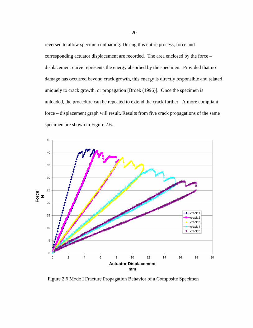
20
reversed to allow specimen unloading. During this entire process, force and
corresponding actuator displacement are recorded. The area enclosed by the force –
displacement curve represents the energy absorbed by the specimen. Provided that no
damage has occurred beyond crack growth, this energy is directly responsible and related
uniquely to crack growth, or propagation [Broek (1996)]. Once the specimen is
unloaded, the procedure can be repeated to extend the crack further. A more compliant
force – displacement graph will result. Results from five crack propagations of the same
specimen are shown in Figure 2.6.
0
5
10
15
20
25
30
35
40
45
0 2 4 6 8 10 12 14 16 18 20
Actuator Displacementmm
Fo
rce
N
crack 1
crack 2
crack 3
crack 4
crack 5
Figure 2.6 Mode I Fracture Propagation Behavior of a Composite Specimen

21
Data Reduction Methods
A common method to evaluate mode I fracture toughness is to simply calculate
the energy a specimen has absorbed during loading and unloading and divide that
quantity by the crack damage area. The crack damage area in the case of a DCB
specimen is the width of the specimen multiplied by the propagated crack length.
The Energy method used to calculate mode I fracture toughness[Broek (1997)] can be
written as:
where
SE is the dissipated energy, numerically integrated from the force – displacement
curve, b is the specimen width, as shown in Figure 2.5,
af is the final crack length and ao is the initial crack length, as shown in Figure 2.5.
This is the most fundamental method for acquiring a GI value from experimental
data. Other methods are available to evaluate GI. One such method is the modified beam
theory method. This method (2.3), like the area method, doesn’t require material
properties to be known a priori.
ba
PG I 2
3 δ= (2.3)
)( ifI aab
SEG
−= (2.2)
22
where
P is load corresponding to initial crack onset,
δ is the deflection (actuator displacement) corresponding to initial crack onset,
a is the initial crack length at crack onset (aI in Figure 2.5),
b is the specimen width from Figure 2.5.
It should be noted that this equation is valid anywhere the crack length and corresponding
load and deflection values are known, while crack growth is occurring. The load and
deflection at crack arrest could also be applied to equation (2.3), with the final crack
length used for a. This approach would provide conservative results since it requires a
slight increase in load to regenerate crack growth. This is evident from viewing the
fracture propagation curve in Figure 2.6.
Mode II
Mode II fracture is caused by in plane shear or a sliding motion between two
surfaces. Bending is the load scenario that typically induces mode II fracture. This
failure mode is more prevalent in laminated composites than metals due to the layered
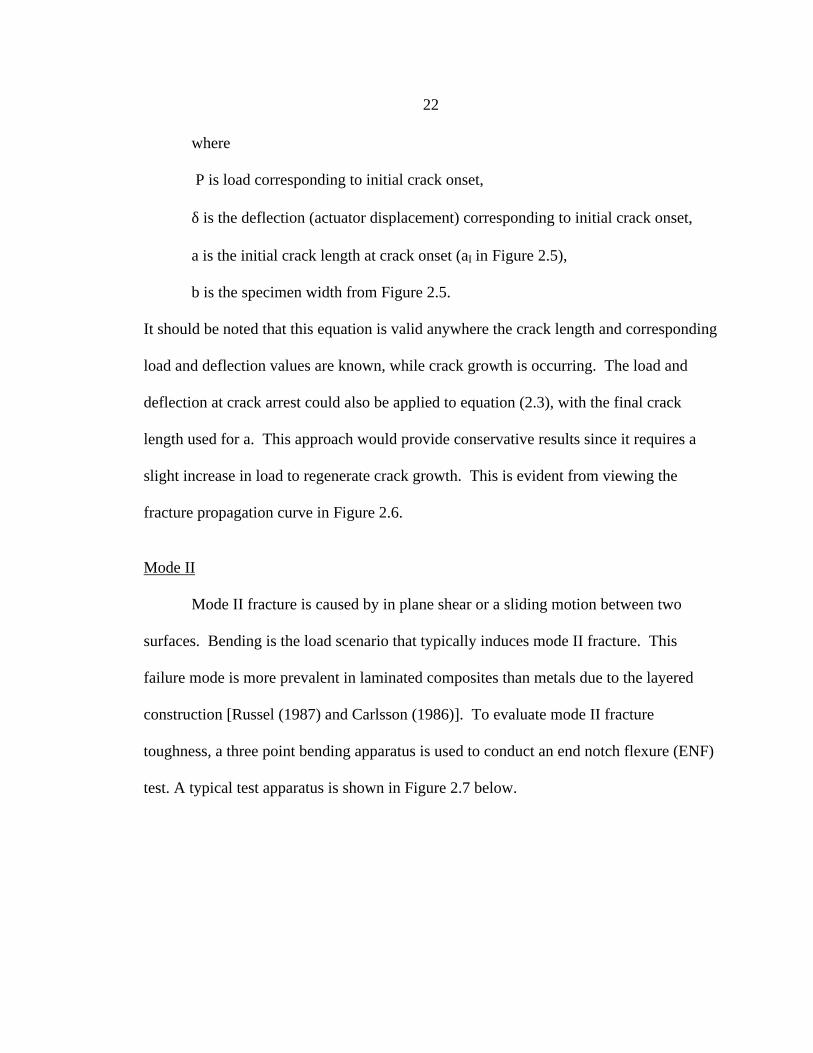
construction [Russel (1987) and Carlsson (1986)]. To evaluate mode II fracture
toughness, a three point bending apparatus is used to conduct an end notch flexure (ENF)
test. A typical test apparatus is shown in Figure 2.7 below.
23
Testing Procedure for ENF Specimen
As with the DCB specimen, an initial crack is required and is typically created
during manufacture with the insertion of a teflon strip. An ENF or end notch flexure
specimen is supported by two rollers, which are separated by about 125 mm. The
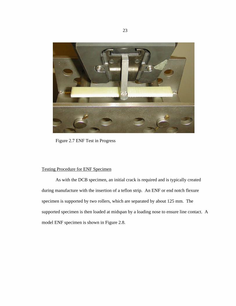
supported specimen is then loaded at midspan by a loading nose to ensure line contact. A
model ENF specimen is shown in Figure 2.8.
Figure 2.7 ENF Test in Progress
24
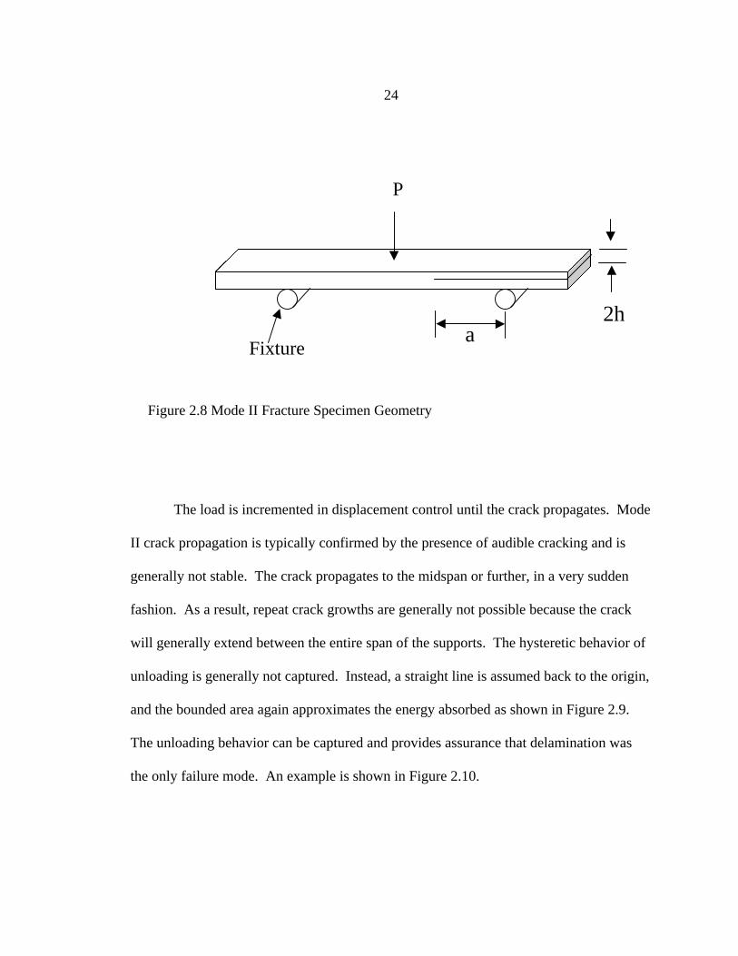
The load is incremented in displacement control until the crack propagates. Mode
II crack propagation is typically confirmed by the presence of audible cracking and is
generally not stable. The crack propagates to the midspan or further, in a very sudden
fashion. As a result, repeat crack growths are generally not possible because the crack
will generally extend between the entire span of the supports. The hysteretic behavior of
unloading is generally not captured. Instead, a straight line is assumed back to the origin,
and the bounded area again approximates the energy absorbed as shown in Figure 2.9.
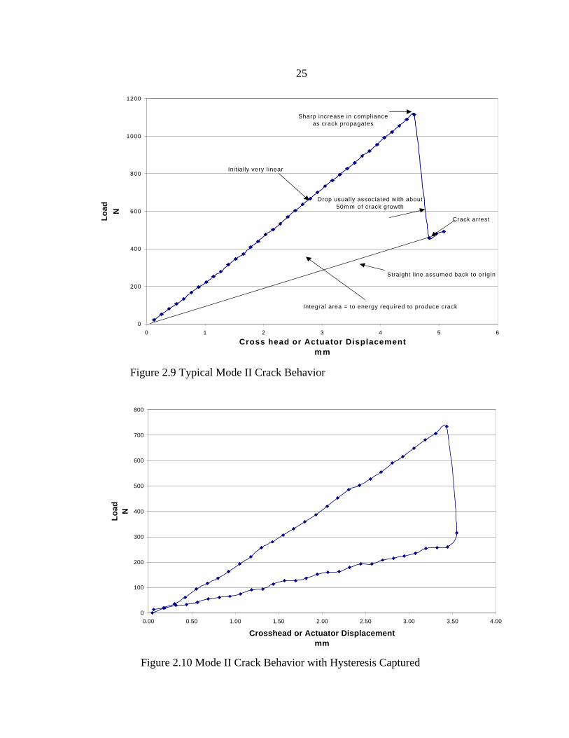
The unloading behavior can be captured and provides assurance that delamination was
the only failure mode. An example is shown in Figure 2.10.
Fixturea
2h
Figure 2.8 Mode II Fracture Specimen Geometry
P
25
Figure 2.9 Typical Mode II Crack Behavior
0
200
400
600
800
1000
1200
0 1 2 3 4 5 6
Cross head or Actuator Displacementm m
Lo
ad N
Initially very linear
Sharp increase in complianceas crack propagates
Drop usually associated with about 50m m of crack growth
Straight line assumed back to origin
Integral area = to energy required to produce crack
Crack arrest
0
100
200
300
400
500
600
700
800
0.00 0.50 1.00 1.50 2.00 2.50 3.00 3.50 4.00
Crosshead or Actuator Displacementmm
Lo
ad N
Figure 2.10 Mode II Crack Behavior with Hysteresis Captured

26
)32(2
933
22
aLw
CaPGII +
= (2.4)
Data Reduction Methods
As in the case of mode I type fracture, the driving element of crack growth is
strain energy. The energy method, equation (2.2), is valid for mode II fracture as well.
The load displacement data can be integrated and divided by the crack damage area to
calculate a GII or mode II fracture toughness.
There is another method available to evaluate GII that is based on beam theory.
This method is called the compliance method. The following series of equations
demonstrate the use of this method [Cairns (1992) and Carlsson and Gillespie (1986)].
where P is the critical load or the force at crack initiation,
C is the compliance of a simple supported beam with a crack extending to one,
edge of length (a),
a is the initial crack length,
w is the width of the specimen,
L is the span length of the specimen.
The compliance (C) can be found by
where E is the elastic modulus and h is half of the total specimen thickness.
3
33
8
32
Ewh
aLC
+= (2.5)
27
A simplified expression for the mode II fracture toughness that neglects shear
contributions is as follows:
Finite Element Theory
The finite element (FEA) method essentially solves the basic spring equation for
segmented regions of a larger body. Then secondary quantities such as strain and stress
are derived from approximation functions and basic constitutive relations. This method
is an approximation that generally provides improved results as the number of regions or
elements used to represent a body is increased. This is increased subdivision is called
mesh refinement.
Benefits
The role of finite element analysis is potentially unlimited. Finite element
simulations are generally used to model experimental phenomena. In the case of costly
experiments with limited material and facilities, finite element simulations can reduce the
number of iterations required to perfect experimental procedures. The primary function
of FEA is modeling complex geometries that can not easily be tested or represented by
simpler methods. Modeled stresses can be compared to material strengths to predict
failure. Other forms of failure such as buckling and fracture can be modeled as well.
32
22
16
9
hEw
aPGII ⋅
⋅=
(2.6)

28
Models and Modeling Procedure
A model is simply a representation of a behavior. Where possible, 2-D
simulations were used to conserve computer resources. Symmetry was employed to
model half or quarter specimens, which also conserved on elements and computer
resources.
Depending on the FEA code that is employed the procedure may vary. However,
the following procedure is consistent with most texts and works well with ANSYS code
[ANSYS (1998)].
1. Generate geometry of problem or structure being investigated. Isolate
behavior that is to be captured, because some simplification may be
implemented in the model to conserve computer resources. 1-D, 2-D, or 3-D
approximations can be used where appropriate.
2. Choose an interpolation function or element type that best represents the
loading conditions, constraints, and material behavior that occurs.
3. Assign constitutive properties or material properties such as elastic moduli,
Poisson’s ratios, and shear moduli. For composite materials these parameters
can vary depending on the laminate’s material directions or architecture.
4. Mesh the geometry with the chosen elements. Some strategy is necessary to
maintain a good aspect ratio and to provide adequate resolution to model
physical behavior.
5. Boundary conditions or constraints should be applied next. This step is
probably the most difficult step to apply accurately.
29
6. Apply loads in the form of forces, pressures, moments, etc.
7. Solve model for primary unknowns, which are typically nodal forces and
displacements. Calculate secondary quantities such as strains and stresses.
8. Interpret results and evaluate convergence by increasing elemental divisions,
increasing order of existing elements, or by adding integration points at
locations of high gradient. Additionally FEA solutions should be compared to
experimental findings or rudimentary analytical solutions. In this study, FEA
solutions were typically validated by experimental findings.
Step 1 Geometry Development
Most of the models constructed for the case studies evaluated were two-
dimensional approximations. Strength or Fracture type failure was being modeled and
parametric models were constructed and used to evaluate stresses or fracture
Step 2 Element Choice
Interpolation functions are used to represent behavior internal to each element.
One or more elements are then used to mathematically represent a structure and its
behavior. Typically, in 2-D simulations ANSYS plane82 8 noded elements were utilized.
This element type provides quadratic approximation capabilities. Both plane strain and
plane stress options were implemented.
Plane strain assumes that when deformation is completely restricted in the z
direction. In response to this restriction, there is a stress in the z direction. The loading is
30
biaxial and no shear stresses result. This assumption typically produces conservative
results, or predicts larger than expected stresses.
Plane stress is useful for modeling relatively thin cross-sections. For plane stress
it is assumed that the strain in the z direction is completely unrestricted so that the stress
in the z direction is 0. Out of plane shear stresses are neglected also in this case.
In 3-D simulations, continuum type elements were used. The ANSYS versions of
these elements that were used in this study are solid45 and solid95. They are typically
referred to as brick elements.
The solid45 element is an eight noded brick element that uses a linear
approximation to represent variations in displacement and force. It is composed of 8
corner nodes, where each node has 3 degrees of freedom. The 3 degrees of freedom are
translations in each of the three dimensions. A special version of this element type is the
solid46 element, which allows for layered properties throughout the element.
The solid95 is a 20 noded brick element and uses a quadratic approximation
function. However this element has 2.5 times as many degrees of freedom as the solid45,
which increases computation time.
A special class of finite elements are available that represent sliding at a
boundary. These elements are generically referred to as contact elements. Sliding and
contact surfaces can be modeled and friction can be accounted for with these elements.
Contact elements were required for the mode II fracture simulations due to the sliding at
the shear induced crack initiation.
31
ANSYS has several contact elements available. The contact169 and target171
elements are specially adapted for two-dimensional surface-to-surface contact. These
elements are capable of handling motion along curved constraints and account for friction
at the sliding interface. Additionally, with these elements both sliding surfaces can be
deformable and possess elastic properties. Other variations of contact elements are
available for different applications.
Step 3 Constitutive Properties
Constitutive properties are material properties such as elastic modulus, Poisson’s
ratio, shear modulus, thermal conductivity, density, and other properties that relate to the
behavior being modeled. For composites, the elastic properties are not always the same
in each direction. For the interlaminar fracture simulations an equivalent modulus or
material stiffness was used. This is called a smeared elastic modulus, and is generally
only used when the transverse properties are not directly related to the behavior
simulated.
Step 4 Meshing
Meshing is simply the process of discretizing a given geometry into elements.
The density of the elements should increase where change is occurring most. In fracture
analysis the element density is always greatest around the crack and the crack front. This
is often called the a/da ratio, which is the crack length divided by the amount of element
divisions.

32
Step 5 and 6 Application of Constraints and Loads
In the case of solid mechanics or structural models, displacement boundary
conditions are generally used. Translations and rotations were restricted to simulate the
constraints on the actual structure. A force was typically applied to represent the load
that would promote crack growth or cause stress failure. When the models were used to
verify experimental behavior the force responsible for crack initiation was used. This is
referred to as the critical load, or load that initiated a mode of failure.
Step 7 and 8 Solution and Results
Primary unknowns are forces and displacements. These values are solved for and
then used to derive strain and stress. Generally, contour stress plots can be used to locate
local high stress regions. Stress should be inspected on an elemental basis, and an
appropriate failure criterion can be applied. Stiffness requirements can also be evaluated
by inspecting displacements at key locations. Special techniques are available to model
fracture and delamination and are discussed.
Finite Element as Related to Fracture Mechanics
There are three basic approaches for the assessment of fracture toughness using
finite element analysis. The stress intensity, strain energy release rate, and the J integral
are methods available [ANSYS (1998)]. Typically, the stress intensity approach is not
used for use with composites, because composites are not isotropic and this complicates
the analysis [Sun (1997)]. The strain energy release rate methods work well with
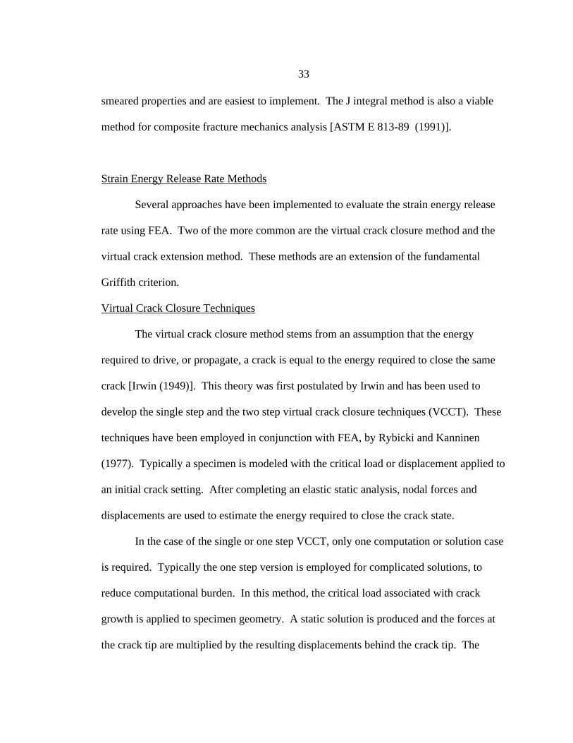
33
smeared properties and are easiest to implement. The J integral method is also a viable
method for composite fracture mechanics analysis [ASTM E 813-89 (1991)].
Strain Energy Release Rate Methods
Several approaches have been implemented to evaluate the strain energy release
rate using FEA. Two of the more common are the virtual crack closure method and the
virtual crack extension method. These methods are an extension of the fundamental
Griffith criterion.
Virtual Crack Closure Techniques
The virtual crack closure method stems from an assumption that the energy
required to drive, or propagate, a crack is equal to the energy required to close the same
crack [Irwin (1949)]. This theory was first postulated by Irwin and has been used to
develop the single step and the two step virtual crack closure techniques (VCCT). These
techniques have been employed in conjunction with FEA, by Rybicki and Kanninen
(1977). Typically a specimen is modeled with the critical load or displacement applied to
an initial crack setting. After completing an elastic static analysis, nodal forces and
displacements are used to estimate the energy required to close the crack state.
In the case of the single or one step VCCT, only one computation or solution case
is required. Typically the one step version is employed for complicated solutions, to
reduce computational burden. In this method, the critical load associated with crack
growth is applied to specimen geometry. A static solution is produced and the forces at
the crack tip are multiplied by the resulting displacements behind the crack tip. The
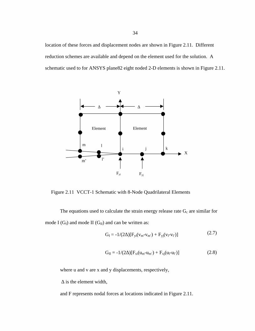
34
location of these forces and displacement nodes are shown in Figure 2.11. Different
reduction schemes are available and depend on the element used for the solution. A
schematic used to for ANSYS plane82 eight noded 2-D elements is shown in Figure 2.11.
The equations used to calculate the strain energy release rate Gc are similar for
mode I (GI) and mode II (GII) and can be written as:
GI = -1/(2∆)[Fyi(vm-vm’) + Fyj(vl-vl’)]
GII = -1/(2∆)[Fxi(um-um’) + Fxj(ul-ul’)]
where u and v are x and y displacements, respectively,
∆ is the element width,
and F represents nodal forces at locations indicated in Figure 2.11.
∆ ∆
Y
X
m li j k
m’ l’
FyjFyi
Element Element
Figure 2.11 VCCT-1 Schematic with 8-Node Quadrilateral Elements
(2.7)
(2.8)
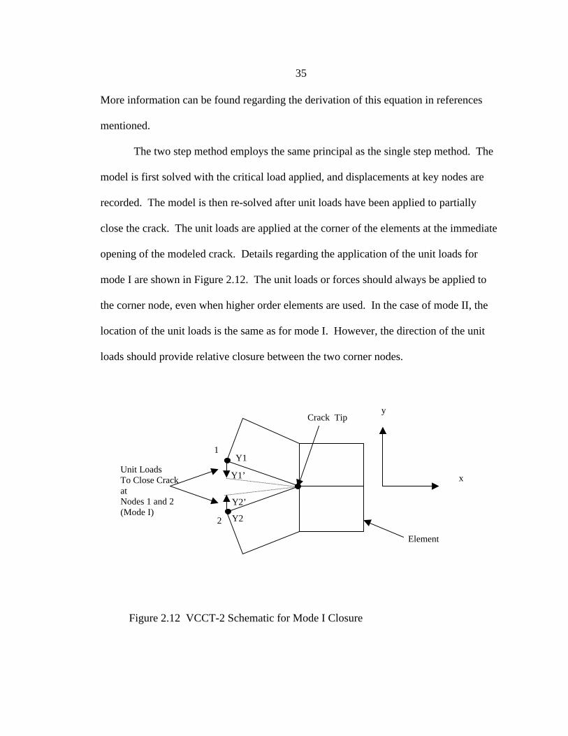
35
More information can be found regarding the derivation of this equation in references
mentioned.
The two step method employs the same principal as the single step method. The
model is first solved with the critical load applied, and displacements at key nodes are
recorded. The model is then re-solved after unit loads have been applied to partially
close the crack. The unit loads are applied at the corner of the elements at the immediate
opening of the modeled crack. Details regarding the application of the unit loads for
mode I are shown in Figure 2.12. The unit loads or forces should always be applied to
the corner node, even when higher order elements are used. In the case of mode II, the
location of the unit loads is the same as for mode I. However, the direction of the unit
loads should provide relative closure between the two corner nodes.
Element
x
Crack Tip
Unit LoadsTo Close CrackatNodes 1 and 2(Mode I)
1
2
y
Y1
Y1’
Y2
Y2’
Figure 2.12 VCCT-2 Schematic for Mode I Closure

36
The initial displacements are used in accordance with the reduced displacements
from the unit load case to evaluate Gc. The equation for this operation follows:
where Xi and Yi are displacements at nodes i,
And X’ and Y’ are displacements at the same nodes after the unit loads have been
applied.
Crack Extension Techniques
The crack extension technique uses total strain energy stored by the specimen at
two states to find the energy required to produce crack growth. Typically the first
solution case is with the critical load or displacement applied that initiated crack
propagation. The second solution case is evaluated with the same load or displacement,
and the crack is extended by either a single node or an element. The residual load or
displacement at crack arrest and corresponding crack length could also be used for the
)(2
)()(
)(
2'
1'
21
221
widthElement
YYYY
YY
GI
−−−−
= (2.9)
)(2
)()(
)(
2'
1'
21
221
widthElement
XXXX
XX
GII
−−−−
=(2.10)
37
second state. The total strain energy for the second case is subtracted from the first, and
divided by the crack damage area. The method can be expressed as:
where U is the total strain energy,
a is the initial crack length,
∆a is the length of crack extension,
and b is the specimen width.
A variation of this technique was developed as part of this study, which simply uses the
final known crack length and corresponding displacement or load for the energy at the
second state.
The FEA methods outlined can be applied to structures and used as a predictive
tool. These methods require material properties such as Gc to be known. The
experimental procedures used to obtain these properties for mode I and and mode II were
presented. Ultimately before these FEA techniques are used they should be validated. In
this study the experimental test conditions were modeled and compared to experimental
results obtained by traditional means. While it is suggested that these models be
expanded to more complex substructures and structures, such activity exceeds the scope
of this study.
)( ab
UUG aaa
∆−
= ∆+ (2.11)

38
CHAPTER 3
INTERLAMINAR FRACTURE CHARACTERIZATION PROCESS
Basic experimental procedures and analytical techniques have been presented.
This chapter addresses the formulation of a fracture toughness optimization process,
incorporating experimental and analytical procedures into a methodology. Industry needs
are summarized, tips and tradeoffs are discussed, and design processes are presented.
Needs
The two most basic needs in current composite manufacturing industries are:
1. Understand the importance of interlaminar fracture of composites.
2. Balance strength and interlaminar fracture toughness and other properties as
well as cost.
To meet these needs it is necessary to:
• Establish testing methodology to evaluate strength and fracture toughness.
• Employ basic data reduction techniques and methods to evaluate material
performance. Additionally inspection techniques should be utilized to
interpret failure modes and reasons for limiting performance of laminated
architectures.
• Develop screening processes to reduce full scale testing and associated
expenses. Screening processes can be an incremental evolution of tests.

39
• Implement FEA fracture techniques as modeling tool to understand and
minimize fracture or delamination failures with Gc material properties.
Optimization
It has been established that structures and their constituent materials should
satisfy strength and fracture toughness requirements. In the case of homogeneous
isotropic materials, strength and fracture toughness are often inversely proportional.
Altering the micro-structure of steel and other metals to enhance strength generally
reduces the fracture toughness or makes the material more brittle.
The structure of a composite material is based on a number of variables. Each
combination of resin system, fiber type, fiber volume, and manufacturing method affect
and alter the strength and fracture performance. It is then necessary to conduct a
constrained optimization evaluation to achieve the best blend of properties. Such an
evaluation will assure that the material does not have excessive strength at the expense of
inadequate fracture toughness.
Fracture Toughness Tips and Tradeoffs
Alterations can be made to constituent materials of a composite to improve
fracture and delamination performance. Often some sacrifice is made for the
improvement. Suggestions are offered that can help improve fracture performance. The
primary elements affecting the delamination resistance are: the resin system used,
architecture and fibers, and inhomogeneities. A more detailed overview of factors that
relate to fracture toughness performance is provided in this section.
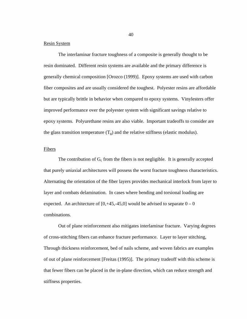
40
Resin System
The interlaminar fracture toughness of a composite is generally thought to be
resin dominated. Different resin systems are available and the primary difference is
generally chemical composition [Orozco (1999)]. Epoxy systems are used with carbon
fiber composites and are usually considered the toughest. Polyester resins are affordable
but are typically brittle in behavior when compared to epoxy systems. Vinylesters offer
improved performance over the polyester system with significant savings relative to
epoxy systems. Polyurethane resins are also viable. Important tradeoffs to consider are
the glass transition temperature (Tg) and the relative stiffness (elastic modulus).
Fibers
The contribution of Gc from the fibers is not negligible. It is generally accepted
that purely uniaxial architectures will possess the worst fracture toughness characteristics.
Alternating the orientation of the fiber layers provides mechanical interlock from layer to
layer and combats delamination. In cases where bending and torsional loading are
expected. An architecture of [0,+45,-45,0] would be advised to separate 0 – 0
combinations.
Out of plane reinforcement also mitigates interlaminar fracture. Varying degrees
of cross-stitching fibers can enhance fracture performance. Layer to layer stitching,
Through thickness reinforcement, bed of nails scheme, and woven fabrics are examples
of out of plane reinforcement [Freitas (1995)]. The primary tradeoff with this scheme is
that fewer fibers can be placed in the in-plane direction, which can reduce strength and
stiffness properties.
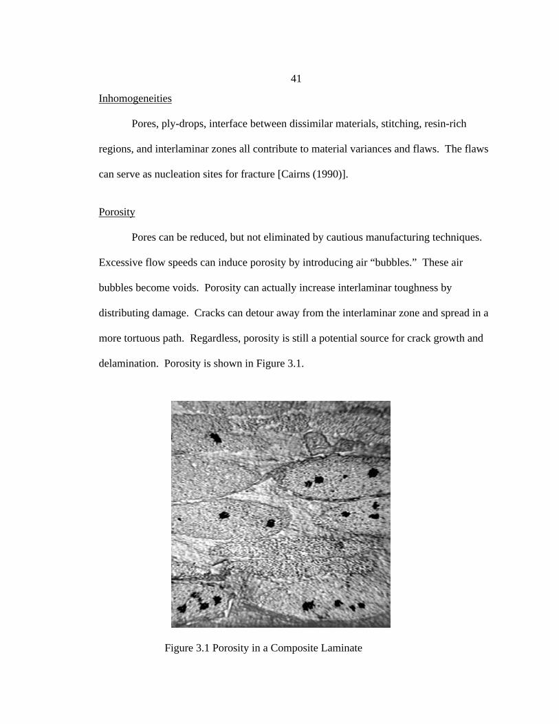
41
Inhomogeneities
Pores, ply-drops, interface between dissimilar materials, stitching, resin-rich
regions, and interlaminar zones all contribute to material variances and flaws. The flaws
can serve as nucleation sites for fracture [Cairns (1990)].
Porosity
Pores can be reduced, but not eliminated by cautious manufacturing techniques.
Excessive flow speeds can induce porosity by introducing air “bubbles.” These air
bubbles become voids. Porosity can actually increase interlaminar toughness by
distributing damage. Cracks can detour away from the interlaminar zone and spread in a
more tortuous path. Regardless, porosity is still a potential source for crack growth and
delamination. Porosity is shown in Figure 3.1.
Figure 3.1 Porosity in a Composite Laminate
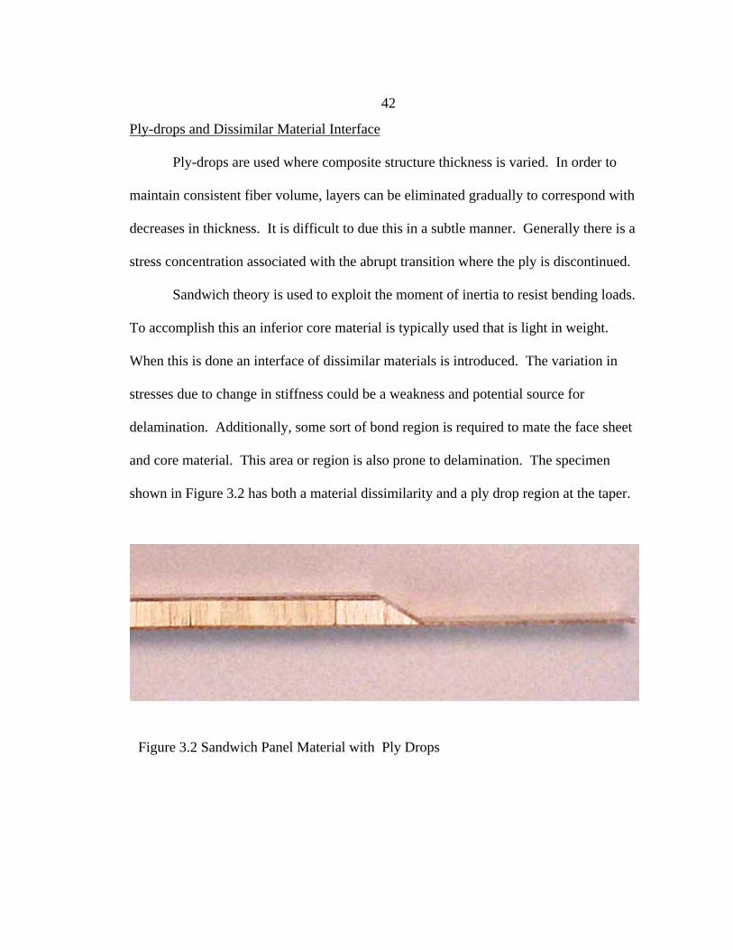
42
Ply-drops and Dissimilar Material Interface
Ply-drops are used where composite structure thickness is varied. In order to
maintain consistent fiber volume, layers can be eliminated gradually to correspond with
decreases in thickness. It is difficult to due this in a subtle manner. Generally there is a
stress concentration associated with the abrupt transition where the ply is discontinued.
Sandwich theory is used to exploit the moment of inertia to resist bending loads.
To accomplish this an inferior core material is typically used that is light in weight.
When this is done an interface of dissimilar materials is introduced. The variation in
stresses due to change in stiffness could be a weakness and potential source for
delamination. Additionally, some sort of bond region is required to mate the face sheet
and core material. This area or region is also prone to delamination. The specimen
shown in Figure 3.2 has both a material dissimilarity and a ply drop region at the taper.
Figure 3.2 Sandwich Panel Material with Ply Drops
43
Interlaminar Zone and Other Inhomogeneities
Stitching, resin rich regions and the interlaminar zone itself are all
inhomogeneities. The interlaminar zone is a region or layer of unreinforced material
between strata of fibers or fabric. This is a specific case of a resin rich region. A resin
rich region is any place where the fibers and resin are not distributed evenly. All
laminated composites possess resin rich regions and interlaminar zones due to the nature
of their construction. A good example of a resin rich region is shown in Figure 3.3.
Avoiding the introduction of the inhomogeneities discussed, and using a resin
with infinite toughness and bondability would eliminate the need for the fracture
mechanic procedures and the delamination analysis techniques discussed. At this point,
this is not possible, so a means to account for, quantify, and improve fracture
Figure 3.3 Resin Rich Region in a Laminated Composite

44
performance is required. The solution proposed is an engineering design process for
composite candidate materials.
Prediction and Screening Approach
Two approaches were investigated, predictive modeling and screening. Failure of
a structure due to fracture and delamination can be modeled. The methods outlined can
be employed to determine the delamination resistance Gc of a material. The strain energy
release rate (SERR) or Gc is a material property that can then be used to evaluate
maximum allowable load for a structure given a flaw size and location. Conversely,
given an operating load a maximum flaw size can also be determined and inspected for.
Local and global analysis schemes are available and mixed mode type analysis is
achievable with the FEA methods provided. The crack closure and crack extension
techniques work well for 2-D structures where the type of damage is known. Without
prior knowledge of the damage and location these techniques become unwieldy.
Additionally, as the architecture is modified to combat fracture or delamination failure,
modeling can become more complex.
However, provided that a database of material properties was gathered, these
materials could be compared at a fundamental level. From simple experiments, elastic
modulus, tensile strength, Tg, GI, and GII properties can be obtained. In the case where
analytical modeling is not reasonably possible, the best material candidate can be selected
and used based on material parameter evaluations. In this case a screening approach is
taken. Additional testing of substructures and incremental or evolutionary experimental
development can also be used. This is where experiments are performed to evaluate

45
specific structural behavior. Before either a prediction or screening approach can be
taken, a database plan needs to be established.
Database
A database is simply a compilation of data or information. In this case a database
would consist of pertinent material properties of a given material or composite.
Databases can range in size; MSU in an effort with the D.O.E. [Mandell et al (1997)], has
generated a substantial database in an effort to ascertain composite properties for wind
turbine blades. Ideally, companies developing composites should emulate this effort on a
smaller scale.
The primary reason for this database development is to provide an aid in the
selection of resins, fibers, and other architectural components. Most of the industry has
embraced the database philosophy for materials, but should consider extending it to
include interlaminar fracture properties, for composites. Once a database has been
established both screening and analysis techniques are feasible for material selection and
architecture development. A process that could be used to establish a database is shown
in Figure 3.4.
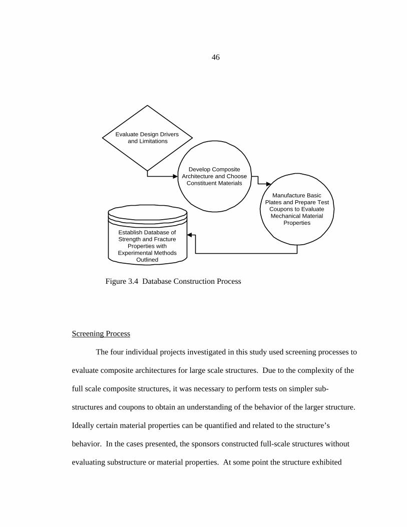
46
Screening Process
The four individual projects investigated in this study used screening processes to
evaluate composite architectures for large scale structures. Due to the complexity of the
full scale composite structures, it was necessary to perform tests on simpler sub-
structures and coupons to obtain an understanding of the behavior of the larger structure.
Ideally certain material properties can be quantified and related to the structure’s
behavior. In the cases presented, the sponsors constructed full-scale structures without
evaluating substructure or material properties. At some point the structure exhibited
Figure 3.4 Database Construction Process
Develop CompositeArchitecture and Choose
Constituent Materials
Manufacture BasicPlates and Prepare Test
Coupons to EvaluateMechanical Material
Properties
Establish Database ofStrength and Fracture
Properties withExperimental Methods
Outlined
Evaluate Design Drivers and Limitations

47
unacceptable performance. These unexpected responses lead to a need for increased
understanding of the material properties of the candidate materials and architectures.
Screening Procedure
Screening is simply a process of isolating and comparing properties of something
to aid in the selection. Screening can occur at a material level. Coupons can be
constructed and submitted to appropriate testing to construct a database of pertinent
material properties. At this point, based on limiting elements of design, the best material
can be chosen based on qualitative comparison of quantified properties. With this
approach, the behavior of the structure is not confidently known. However, at minimum,
the designer has a better chance of choosing the best material to manufacture the structure
and meet its in service needs.
Various experiments can be developed to address potential problems and
behavior. Simple substructures can be constructed of rival materials and tested at
incremental levels. Confidence can then be gained at various levels regarding the
performance of the material. An evolution of successfully constructed and tested sub-
structures can then lead to a successful construction and performance of the final
structure as shown in Figure 3.5.
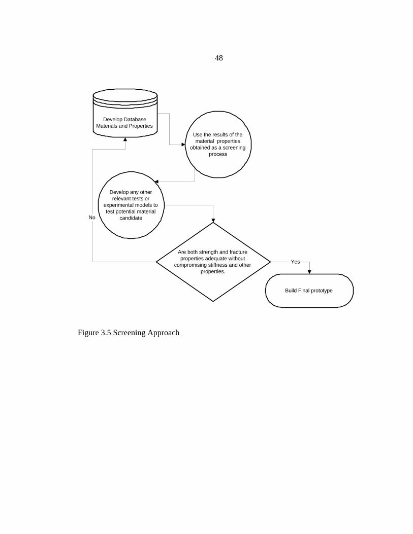
48
Are both strength and fractureproperties adequate without
compromising stiffness and otherproperties.
Use the results of thematerial properties
obtained as a screeningprocess
Develop any otherrelevant tests or
experimental models totest potential material
candidate
Yes
Build Final prototype
Develop DatabaseMaterials and Properties
No
Figure 3.5 Screening Approach

49
Prediction Approach
The roles of finite element analysis (FEA) were discussed in the previous chapter.
This analytical technique has the potential to be used as a predictive tool. With the
inclusion of key constitutive and strength properties, models can be constructed that
represents the behavior and failure of structures. These models are not prophecy and
need to be “anchored” or compared to other analysis and generally experimental results
to establish confidence. When FEA models are accurate, significant expense and
resources can be saved. Ultimately FEA and other analysis techniques can be used to
forecast the performance of a potential structure. The performance typically includes
stiffness and strength capabilities.
Analytical methods capable of predicting fracture and delamination in test
coupons have been presented. Significant effort has been invested to extend these
methods to substructures and ultimately to structures. The goal of obtaining material
properties at a coupon level and using these values to model structural behavior has been
a focus of the Composite Technology Team at Montana State University (MSU).
Currently, predicting delamination in complex structures is not a simple science. To
accurately model fracture in these situations requires some additional development.
Some advancement was made with composite T sections by Morehead (2000) and
Haugen (1998). In these studies, FEA models were used to model and predict the
delamination of composite T sections. From these investigations a basic methodology
was formed and is presented in Figure 3.4. This process ensures strength and stiffness
performance and attempts to evaluate fracture performance at a structural level.
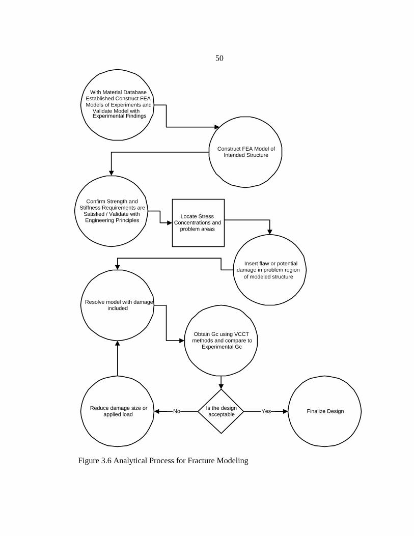
50
With Material DatabaseEstablished Construct FEAModels of Experiments and
Validate Model withExperimental Findings
Insert flaw or potentialdamage in problem region
of modeled structure
Resolve model with damageincluded
Obtain Gc using VCCTmethods and compare to
Experimental Gc
Locate StressConcentrations and
problem areas
Confirm Strength andStiffness Requirements are
Satisfied / Validate withEngineering Principles
Is the designacceptable
YesReduce damage size or
applied loadFinalize Design
Construct FEA Model ofIntended Structure
No
Figure 3.6 Analytical Process for Fracture Modeling

51
Composite Design
A systematic approach to designing laminated architectures that ensures adequate
strength and resistance to interlaminar fracture is offered. These following steps should
be followed to produce an optimized strong and tough composite. The process is as
follows.
1. Apply analytical methods available to evaluate forces and stresses on
component desired. Establish and evaluate potential design drivers and
limitations.
2. With the aid of classical lamination theory, develop an architecture scheme
that best addresses loading conditions. Details such as fiber type, resin
system, fiber volume, and fiber orientation should be considered at this stage.
3. With a set of architecture candidates established, the initial construction of
simple plates should be conducted. Specimens can be sectioned from these
plates, which can then be subjected to tensile testing, mode I fracture testing,
static flexure testing, etc. Some considerations to effectively address
interlaminar fracture toughness are listed below.
Ø Mode I tests are generally used as a fundamental characterization of
fracture toughness.
Ø In applications where bending type loading is present, mode II should
be evaluated also. GII is not always directly proportional to GI. This
type of failure is common in composites and should not be overlooked.
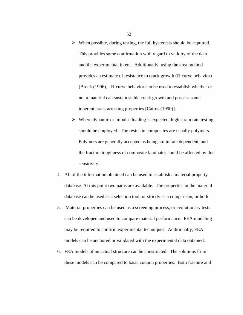
52
Ø When possible, during testing, the full hysteresis should be captured.
This provides some confirmation with regard to validity of the data
and the experimental intent. Additionally, using the area method
provides an estimate of resistance to crack growth (R-curve behavior)
[Broek (1996)]. R-curve behavior can be used to establish whether or
not a material can sustain stable crack growth and possess some
inherent crack arresting properties [Cairns (1990)].
Ø Where dynamic or impulse loading is expected, high strain rate testing
should be employed. The resins in composites are usually polymers.
Polymers are generally accepted as being strain rate dependent, and
the fracture toughness of composite laminates could be affected by this
sensitivity.
4. All of the information obtained can be used to establish a material property
database. At this point two paths are available. The properties in the material
database can be used as a selection tool, or strictly as a comparison, or both.
5. Material properties can be used as a screening process, or evolutionary tests
can be developed and used to compare material performance. FEA modeling
may be required to confirm experimental techniques. Additionally, FEA
models can be anchored or validated with the experimental data obtained.
6. FEA models of an actual structure can be constructed. The solutions from
these models can be compared to basic coupon properties. Both fracture and

53
strength requirements can be optimized. Other properties such as Tg can be
optimized in this fashion as well.
The basic needs presented were shared by four separate projects. Each project
possessed a unique facet or delamination situation. The design processes discussed were
applied to each project to solve individual project needs and to establish confidence in
and the validity of the processes. The following chapters are case study evaluations of
the projects outlined.
In almost all cases the screening comparison path was chosen. However,
significant effort was also focused on the development and application of analytical
techniques and models. This effort was done to advance the technology associated with
the prediction approach. Applying database material properties and FEA analysis as a
predictive tool is ideal, but the confidence associated with these analyses is limited. An
interactive design process that includes incremental screening tests and FEA validation is
most desirable.
54
CHAPTER 4
CASE STUDY ICOMPOSITE AEROFAN BLADE EVALUATION
This project employed a database – screening approach. Basic material properties
were identified that related to structural performance. Experimental procedures were
developed to test these properties for several composite material candidates. These
materials properties and parameters were then compared as a screening process to find
the best suited candidates for potential composite structural architectures. Additionally,
some research was conducted regarding fracture modeling. Numerical mode II
simulations were developed to substantiate and help explain experimental findings. The
numerical study employed several analysis techniques to predict GIIc values. Friction at
the sliding interface was accounted for and results were compared for varying friction
coefficients.
Project Introduction
Traditionally, fan blades for turbofan engines have been constructed from
materials such as titanium, high strength aluminum alloys, and steels. The demand for
reduction in component weight and cost has spurred interest in the use of high strength
composites as alternative materials. Minimizing the weight of the blades in turn reduces
the associated weight of supporting bearings, journals and shaft-mounted components
[Cairns (1999)].
55
Composite materials that have the potential of replacing metals for blade use exist.
However, many of these candidates have trouble passing the “bird strike test” [Weeks
(1998)] and other durability requirements.
Bird impact is a primary design consideration of fan components for turbofan
engines. The actual bird strike test consists of the engine ingesting four 2.5 pound birds in
sequence at operational speeds that would correspond to 85,000 pounds of thrust. The
engine and related components have to be effectively sized to meet the bird strike
requirements. The weak transverse properties of composites have often lead designers to
the continued use of materials such as titanium. Only the GE90 motor is currently
equipped with a composite Aerofan blade. This motor is used to power the Boeing 747
and the details of its architecture and properties are proprietary and unknown. It is
believed that dynamic mode II fracture would be the major cause of blade failure for
composite blades subjected to birdstrike conditions.
Existing Work
To combat the possibility of delamination, significant effort was spent evaluating
through thickness reinforced composites [Jarmon (1998), Naik (1998), and Weeks
(1998)]. Pratt & Whitney conducted several investigations to develop a composite
material that would have improved transverse properties and greater delamination
resistance.
Soft body impact testing was conducted with gelatin bird-like replicas [Weeks
(1998)]. These 110 gram birds were projected at prepared panels at a speed of about
56
400 m/s. Typically the impact energy was increased with incremented impact speeds
until damage formed. The impact conditions were increased further to evaluate damage
tolerance. It was concluded that the stitched laminates possessed an increased damage
tolerance and delamination resistance, but with a reduced initial damage threshold.
Additional investigations were conducted regarding the implementation of micro-
mechanical architectural analysis [Naik (1998)] and mechanical properties of standard 2-
D and 3-D RTM composites [Jarmon (1998)]. The two dimensional (2-D) composites
were standard baseline laminates without through thickness reinforcement. The three
dimensional (3-D) composites were similar but included cross-stitching or weaving to
reduce delamination tendencies. The mechanical properties evaluated were in-plane
tension (strength and modulus), in-plane compression (strength and modulus), and
flexural and shear strengths. Some increase was noted in the tensile and compressive
moduli for 2-D stitched variations. However, all other properties suffered when any
through thickness or layer to layer reinforcement was added.
Some hybrid (S-2 glass-IM7 carbon) reinforced architectures were also produced
and tested. The hybrid versions showed no improvement over the baseline 2-D satin
weave (non-reinforced) carbon fiber epoxy composite.
Full Scale Testing and Need for Screening Process
Bird strikes are a predominant hazard faced by jet engine blades in use. Standard
procedures have been developed to simulate bird collision events using full-scale blade
assemblies as discussed. However, the destructive testing of full-scale assemblies is time-
consuming and costly. A series of test procedures are therefore desired to provide
57
quantitative data for the component materials rather than for the entire composite
structure. A material testing hierarchy would permit refinement of component materials
and related properties. The components fabricated from these materials would be more
likely to pass bird strike tests and meet other in-service durability requirements. A
generalized problem statement to summarize project goals follows.
Problem Statement
Pratt & Whitney, under the DARPA sponsored Affordable Composites for
Propulsion (ACP), has pursued the challenge of developing a composite aircraft engine
fan blade. Toward this goal, Pratt & Whitney needs an economical method of evaluating
mechanical properties of composites. Montana State University was tasked to assist in
this effort by addressing the following tasks.
1. Isolate material properties and characteristics that apply to aerofan bladedesign and typical in service load scenarios.
2. Develop appropriate test methods to evaluate these properties.
3. Present and compare results from testing actual specimens.
4. Make recommendations for modifications of material composition, byproviding actual minimum design specifications.
To address these considerations, a parametric study was performed to evaluate
individual composites. Based on characteristics found, appropriate materials for blade
usage can be selected. Such a study requires a test methodology, experimental results,
and ultimately interpretation of those results: Each of these topics are addressed in
subsequent sections of this case study evaluation.
58
Jet engine aerofan blades must meet very demanding specifications. Among these
are stiffness requirements, tensile strength and various durability requirements. The goal
of this study was to investigate the durability aspects of the candidates provided and
either choose the best candidate for blade design or determine appropriate specifications
to improve durability without sacrificing original design requirements.
Design Drivers and Material Limitations
Durability properties that were investigated fall into two categories: in-and out-of-
plane strength. Often, measures taken to increase interlaminar strength sacrifice in plane
strength. Heavy cross-stitching, for example increases out of plane strength by providing
resistance to delamination. However, in-plane strength is lost when in-plane fibers are
replaced by cross-stitching. Acceptable in-plane and out-of-plane strengths are both
required for impact survival and durability. Delamination is a significant out of plane
mode of failure for composites, and was addressed during testing. In plane metrics
include bending stress, bending modulus, energy absorbed during impact, as well as
threshold and ultimate dynamic strength.
Materials Provided and Specimen Description
To support completion of the stated goals, a small assortment of approximately 40
rectangular specimens and 12 “dog bone” tensile specimens were supplied by Pratt and
Whitney. These specimens were tested, evaluated, and compared. Four distinctly
different compositions were represented in these specimen configurations. Variations
included different degrees of cross-stitching and unstitched versions. The cross-stitched
laminates are generally referred to as ‘3-D composites” and the unstitched are termed “2-
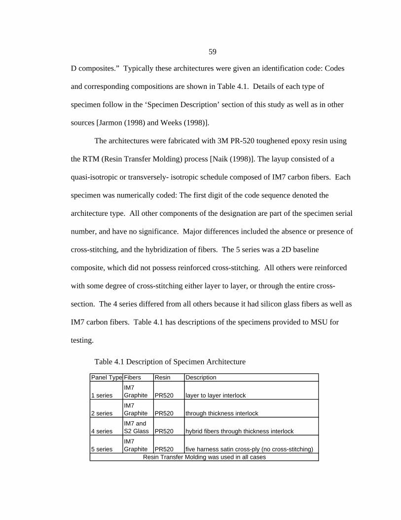
59
D composites.” Typically these architectures were given an identification code: Codes
and corresponding compositions are shown in Table 4.1. Details of each type of
specimen follow in the ‘Specimen Description’ section of this study as well as in other
sources [Jarmon (1998) and Weeks (1998)].
The architectures were fabricated with 3M PR-520 toughened epoxy resin using
the RTM (Resin Transfer Molding) process [Naik (1998)]. The layup consisted of a
quasi-isotropic or transversely- isotropic schedule composed of IM7 carbon fibers. Each
specimen was numerically coded: The first digit of the code sequence denoted the
architecture type. All other components of the designation are part of the specimen serial
number, and have no significance. Major differences included the absence or presence of
cross-stitching, and the hybridization of fibers. The 5 series was a 2D baseline
composite, which did not possess reinforced cross-stitching. All others were reinforced
with some degree of cross-stitching either layer to layer, or through the entire cross-
section. The 4 series differed from all others because it had silicon glass fibers as well as
IM7 carbon fibers. Table 4.1 has descriptions of the specimens provided to MSU for
testing.
Panel Type Fibers Resin Description
1 seriesIM7 Graphite PR520 layer to layer interlock
2 seriesIM7 Graphite PR520 through thickness interlock
4 seriesIM7 and S2 Glass PR520 hybrid fibers through thickness interlock
5 seriesIM7 Graphite PR520 five harness satin cross-ply (no cross-stitching)
Resin Transfer Molding was used in all cases
Table 4.1 Description of Specimen Architecture
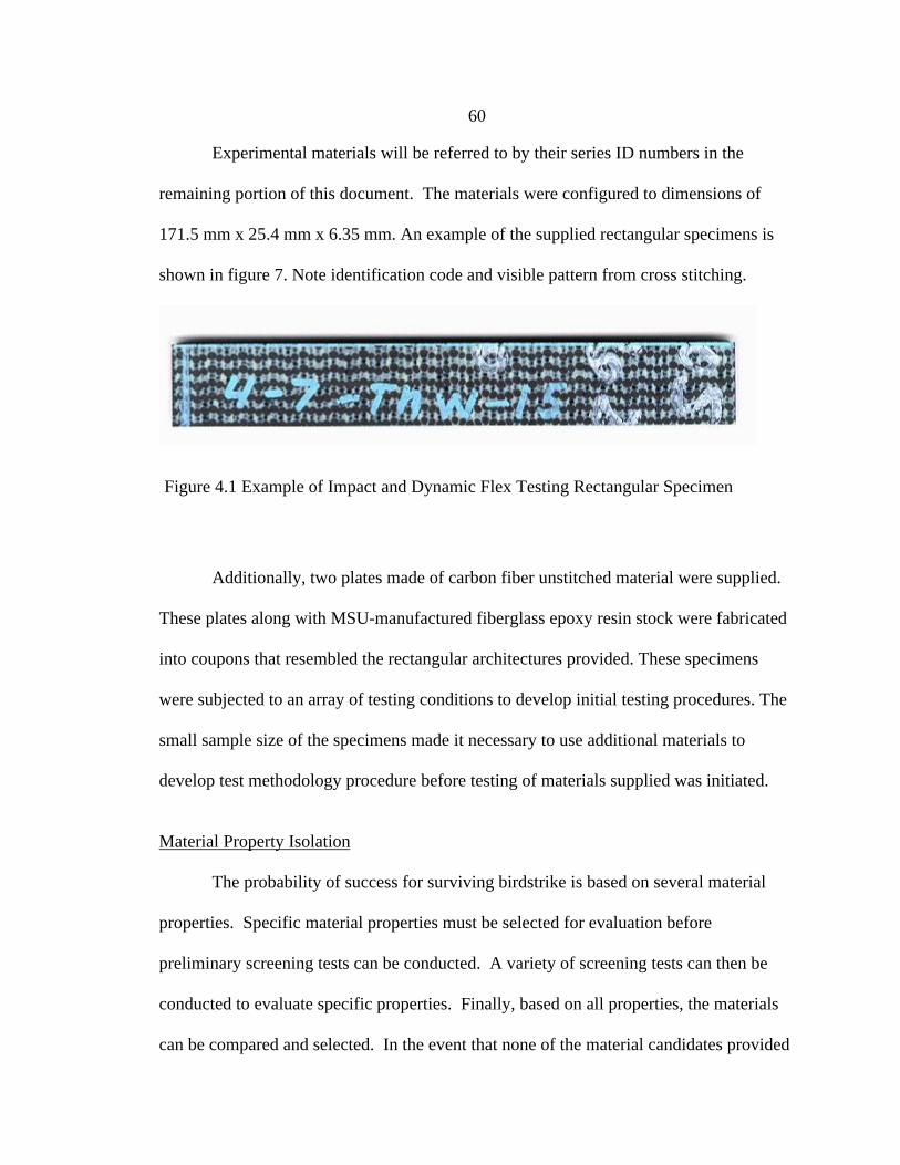
60
Experimental materials will be referred to by their series ID numbers in the
remaining portion of this document. The materials were configured to dimensions of
171.5 mm x 25.4 mm x 6.35 mm. An example of the supplied rectangular specimens is
shown in figure 7. Note identification code and visible pattern from cross stitching.
Additionally, two plates made of carbon fiber unstitched material were supplied.
These plates along with MSU-manufactured fiberglass epoxy resin stock were fabricated
into coupons that resembled the rectangular architectures provided. These specimens
were subjected to an array of testing conditions to develop initial testing procedures. The
small sample size of the specimens made it necessary to use additional materials to
develop test methodology procedure before testing of materials supplied was initiated.
Material Property Isolation
The probability of success for surviving birdstrike is based on several material
properties. Specific material properties must be selected for evaluation before
preliminary screening tests can be conducted. A variety of screening tests can then be
conducted to evaluate specific properties. Finally, based on all properties, the materials
can be compared and selected. In the event that none of the material candidates provided
Figure 4.1 Example of Impact and Dynamic Flex Testing Rectangular Specimen
61
meet minimum requirements, specifications and suggested modifications in architecture
can be developed. Four experiments were chosen to evaluate the material properties that
directly relate to the design drivers discussed. The 3-point bend test or static flexure test
establishes static strength properties and stiffness properties. The dynamic flexure test
evaluates strength properties at high strain rates, while the delamination testing addresses
fracture toughness. The delamination tests conducted were at high strain rates also. The
primary goal with testing is to relate material properties to design drivers. Since bird
strike is the in service threat, dynamic or impact type tests were conducted.
Test Matrix
An array of different tests were required to investigate all of the above mentioned
quantities. No one test could reveal all of these mechanical properties. A test matrix
Table 4.2 was developed that lists candidate identification and tests conducted (where a *
indicates a single test). Specific descriptions of test procedures, equipment used, and the
results are provided in following sections. A description of nomenclature is included
only the first digit relates to the specimen architecture. All other numbers and letters
relate to the specimen identification.
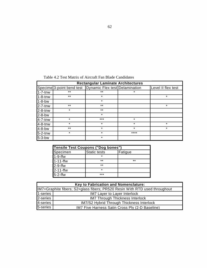
62
Specimen 3-point bend test Dynamic Flex test Delamination Level II flex test1-7-tnw ** ** *1-8-tnw ** * *1-8-bw *2-7-tnw ** ** *2-8-tnw * **2-8-bw *4-7-tnw * *** *4-8-tnw * * * *4-8-bw ** * * *5-2-tnw * * ****5-3-bw *
Tensile Test Coupons ("Dog bones")Specimen Static tests Fatigue1-9-ffw *1-11-ffw ** **2-9-ffw **2-11-ffw *5-2-ffw ***
IM7=Graphite fibers; S2=glass fibers; PR520 Resin With RTD used throughout1-series2-series4-series5-series
IM7/S2 Hybrid Through Thickness InterlockIM7 Five Harness Satin Cross Ply (2-D Baseline)
Rectangular Laminate Architectures
Key to Fabrication and Nomenclature:
IM7 Layer to Layer Interlock IM7 Through Thickness Interlock
Table 4.2 Test Matrix of Aircraft Fan Blade Candidates

63
Experimental Procedures
Based on the expected structural requirements, related material properties to
achieve them, and the test matrix formed, a series of experiments were conducted. Each
test was related to a material property of interest. The material property is explained as
well as the apparatus used, procedure followed, and data reduction methods employed to
evaluate said property.
Basic In-plane and Interlaminar properties
In-plane properties and interlaminar properties were used to characterize the
supplied specimens. In-plane properties included ultimate tensile strength, elastic
modulus, and fatigue life. Interlaminar characteristics were evaluated using mode II type
test methods [Cairns (1992), Russel (1987) and Carlsson (1986)]. Two separate testing
devices were used to obtain the associated properties.
Delamination Mode II Testing
Delamination resistance was evaluated using dynamic mode II testing.
Delamination resistance to impact is considered one of the most significant parameters,
since composites generally possess poor interlaminar fracture properties. Due to the
nature of loads imposed by potential birdstrike, a dynamic version of the mode II fracture
test was conducted. The metric of delamination resistance from this experiment was still
GIIc, but for dynamic loading conditions. This property accounts for any strain rate
dependencies of the material [Cairns (1992)].
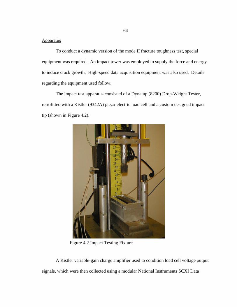
64
Apparatus
To conduct a dynamic version of the mode II fracture toughness test, special
equipment was required. An impact tower was employed to supply the force and energy
to induce crack growth. High-speed data acquisition equipment was also used. Details
regarding the equipment used follow.
The impact test apparatus consisted of a Dynatup (8200) Drop-Weight Tester,
retrofitted with a Kistler (9342A) piezo-electric load cell and a custom designed impact
tip (shown in Figure 4.2).
A Kistler variable-gain charge amplifier used to condition load cell voltage output
signals, which were then collected using a modular National Instruments SCXI Data
Figure 4.2 Impact Testing Fixture
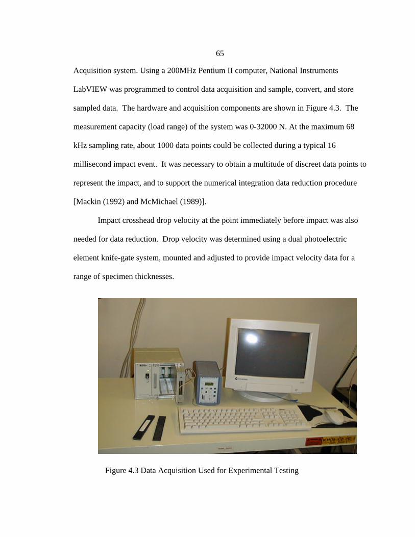
65
Acquisition system. Using a 200MHz Pentium II computer, National Instruments
LabVIEW was programmed to control data acquisition and sample, convert, and store
sampled data. The hardware and acquisition components are shown in Figure 4.3. The
measurement capacity (load range) of the system was 0-32000 N. At the maximum 68
kHz sampling rate, about 1000 data points could be collected during a typical 16
millisecond impact event. It was necessary to obtain a multitude of discreet data points to
represent the impact, and to support the numerical integration data reduction procedure
[Mackin (1992) and McMichael (1989)].
Impact crosshead drop velocity at the point immediately before impact was also
needed for data reduction. Drop velocity was determined using a dual photoelectric
element knife-gate system, mounted and adjusted to provide impact velocity data for a
range of specimen thicknesses.
Figure 4.3 Data Acquisition Used for Experimental Testing
66
A special purpose fixture was designed to support the impact specimens and
prevent translation before or during impact. This fixture supported the specimens in a
simple (three point bending) configuration. The fixture was adjustable to provide a
variety of spans, and possessed enough clearance to allow for deflections of up to 1 inch.
The installed impact fixture is shown in Figure 4.2.
Procedure
Some of the procedure and data reduction techniques are similar to the mode II
fracture toughness methods outlined in Chapter 2. The test specimen geometry is the
same. In this case the initial crack was induced by means of a specially constructed jig
and chisel tool. The material was supplied by the project sponsor and was not
manufactured on site. This made it impossible to incorporate a teflon strip for the initial
flaw or crack. As a result the initial crack was induced with a precision chisel and
guiding fixture.
Typically, in fracture testing, crack fronts can be measured visually with a caliper.
The specimens provided were constructed of IM7 carbon fiber. This dark colored
laminate made it difficult to determine the location of the crack fronts visually. Instead
the crack fronts were located through the use of an ultrasonic transducer. Once located,
they were marked and the distance from the support location to the crack front was
measured with a standard caliper. The initial crack length is critical because the
compliance method for the analysis of GIIc depends solely on the initial crack length.
With the initial crack length, width, thickness, and span length of the specimen
known, it was then supported in test fixture described above. With the aid of an assistant,
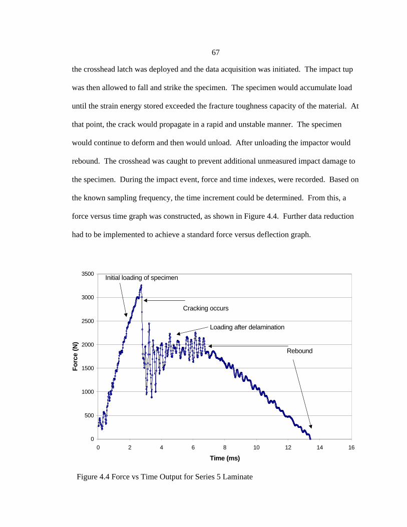
67
the crosshead latch was deployed and the data acquisition was initiated. The impact tup
was then allowed to fall and strike the specimen. The specimen would accumulate load
until the strain energy stored exceeded the fracture toughness capacity of the material. At
that point, the crack would propagate in a rapid and unstable manner. The specimen
would continue to deform and then would unload. After unloading the impactor would
rebound. The crosshead was caught to prevent additional unmeasured impact damage to
the specimen. During the impact event, force and time indexes, were recorded. Based on
the known sampling frequency, the time increment could be determined. From this, a
force versus time graph was constructed, as shown in Figure 4.4. Further data reduction
had to be implemented to achieve a standard force versus deflection graph.
Figure 4.4 Force vs Time Output for Series 5 Laminate
0
500
1000
1500
2000
2500
3000
3500
0 2 4 6 8 10 12 14 16
Time (ms)
Fo
rce
(N)
Initial loading of specimen
Cracking occurs
Loading after delamination
Rebound
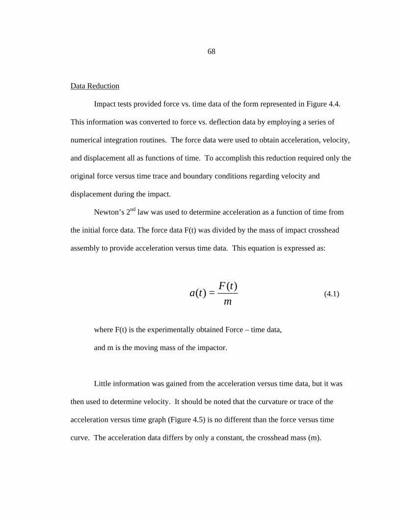
68
Data Reduction
Impact tests provided force vs. time data of the form represented in Figure 4.4.
This information was converted to force vs. deflection data by employing a series of
numerical integration routines. The force data were used to obtain acceleration, velocity,
and displacement all as functions of time. To accomplish this reduction required only the
original force versus time trace and boundary conditions regarding velocity and
displacement during the impact.
Newton’s 2nd law was used to determine acceleration as a function of time from
the initial force data. The force data F(t) was divided by the mass of impact crosshead
assembly to provide acceleration versus time data. This equation is expressed as:
where F(t) is the experimentally obtained Force – time data,
and m is the moving mass of the impactor.
Little information was gained from the acceleration versus time data, but it was
then used to determine velocity. It should be noted that the curvature or trace of the
acceleration versus time graph (Figure 4.5) is no different than the force versus time
curve. The acceleration data differs by only a constant, the crosshead mass (m).
m
tFta
)()( = (4.1)
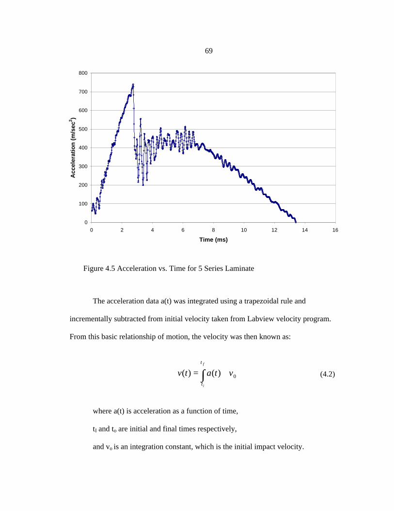
69
The acceleration data a(t) was integrated using a trapezoidal rule and
incrementally subtracted from initial velocity taken from Labview velocity program.
From this basic relationship of motion, the velocity was then known as:
where a(t) is acceleration as a function of time,
tI and to are initial and final times respectively,
and vo is an integration constant, which is the initial impact velocity.
∫ +=f
i
t
t
vtatv 0)()( (4.2)
Figure 4.5 Acceleration vs. Time for 5 Series Laminate
0
100
200
300
400
500
600
700
800
0 2 4 6 8 10 12 14 16
Time (ms)
Acc
eler
atio
n (
m/s
ec2 )
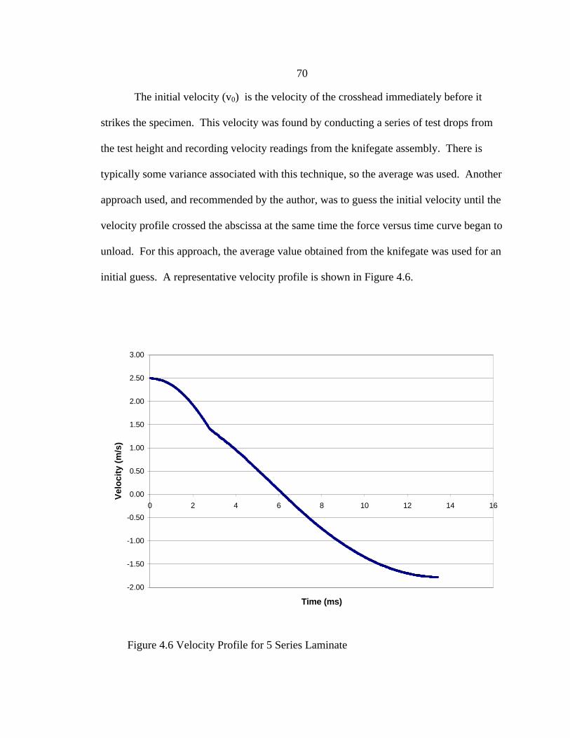
70
The initial velocity (v0) is the velocity of the crosshead immediately before it
strikes the specimen. This velocity was found by conducting a series of test drops from
the test height and recording velocity readings from the knifegate assembly. There is
typically some variance associated with this technique, so the average was used. Another
approach used, and recommended by the author, was to guess the initial velocity until the
velocity profile crossed the abscissa at the same time the force versus time curve began to
unload. For this approach, the average value obtained from the knifegate was used for an
initial guess. A representative velocity profile is shown in Figure 4.6.
-2.00
-1.50
-1.00
-0.50
0.00
0.50
1.00
1.50
2.00
2.50
3.00
0 2 4 6 8 10 12 14 16
Time (ms)
Vel
oci
ty (
m/s
)
Figure 4.6 Velocity Profile for 5 Series Laminate

71
Note the velocity profile crosses the abscissa indicating that the crosshead stops at
bottom dead center and rebounds upward as specimen unloads. Also the negative
rebound velocity is less than initial impact velocity. This indicates that energy has been
lost due to material damage.
Using the surface of the impact candidate as a datum, the velocity data, v(t), can
be integrated and incrementally added to the initial displacement of zero. This was
accomplished with the following relationship:
where v(t) is the velocity as a function of time,
tI and tf are initial and final time respectively,
and d0 is an integration constant equal to 0 or the datum.
The result of this reduction is a displacement vs. time data set (Figure 4.7)
∫ +=f
i
t
t
dtvtd 0)()( (4.3)
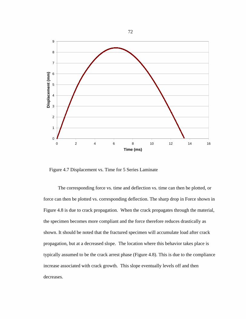
72
The corresponding force vs. time and deflection vs. time can then be plotted, or
force can then be plotted vs. corresponding deflection. The sharp drop in Force shown in
Figure 4.8 is due to crack propagation. When the crack propagates through the material,
the specimen becomes more compliant and the force therefore reduces drastically as
shown. It should be noted that the fractured specimen will accumulate load after crack
propagation, but at a decreased slope. The location where this behavior takes place is
typically assumed to be the crack arrest phase (Figure 4.8). This is due to the compliance
increase associated with crack growth. This slope eventually levels off and then
decreases.
0
1
2
3
4
5
6
7
8
9
0 2 4 6 8 10 12 14 16
Time (ms)
Dis
pla
cem
ent
(mm
)
Figure 4.7 Displacement vs. Time for 5 Series Laminate
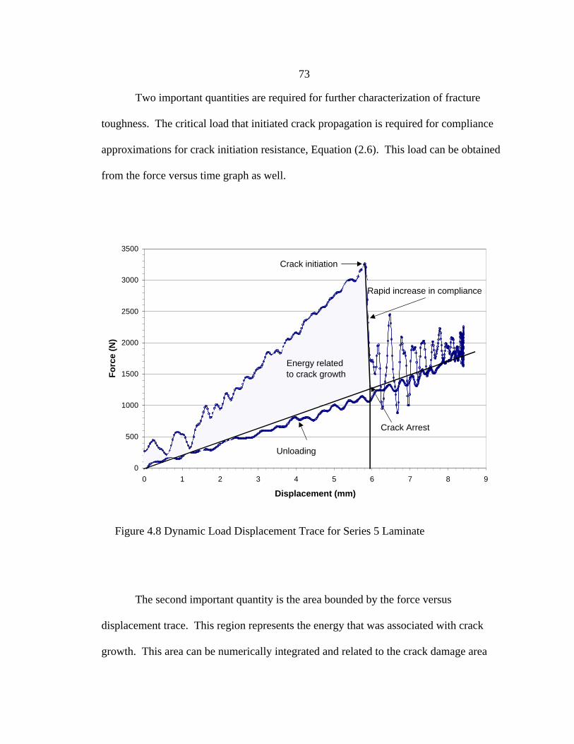
73
Two important quantities are required for further characterization of fracture
toughness. The critical load that initiated crack propagation is required for compliance
approximations for crack initiation resistance, Equation (2.6). This load can be obtained
from the force versus time graph as well.
The second important quantity is the area bounded by the force versus
displacement trace. This region represents the energy that was associated with crack
growth. This area can be numerically integrated and related to the crack damage area
0
500
1000
1500
2000
2500
3000
3500
0 1 2 3 4 5 6 7 8 9
Displacement (mm)
Fo
rce
(N)
Crack initiation
Crack Arrest
Rapid increase in compliance
Energy related to crack growth
Unloading
Figure 4.8 Dynamic Load Displacement Trace for Series 5 Laminate
74
using Equation (2.2). This quantity is typically used as a measure of resistance to crack
growth, not resistance to crack initiation. Generally the area method, Equation (2.2)
yields larger values than the compliance method, Equation (2.6). This difference is due
to fiber bridging and other phenomenon that can act as crack deterents. This type of R
curve or resistance curve behavior is common. Materials which provide reduced Gc
results for the area method relative to the compliance method are generally not good for
durability. This is because without R curve behavior, cracks can grow unstably and
rapidly once they are initiated.
Dynamic Flexure Testing
The dynamic flexure test is used to measure the threshold, or flexural strength,
and the energy absorbed before damage and after damage initiates. The threshold
strength is defined as the flexural stress at which damage initiates. The term tolerance is
used to describe the ability of a material to continue structural performance after
sustaining damage. Threshold strength is the more significant of the two because ideally,
the blade should withstand birdstrike type impact without becoming damaged or
permanently deformed. Typically materials with a considerable threshold exhibited
lower damage tolerances [Cairns and Lagace (1989)]. Since most composites have low
strain to failure values, threshold strengths are viewed as important parameters related to
durability during impact. Of the parameters discussed only the flexural strength obtained
is considered a material property. The energy absorbed before damage and total energy
absorbed during impact can be used to compare materials, but are not considered material
properties.
75
Apparatus
The same apparatus was used for the dynamic flexure testing as was used for the
dynamic delamination testing. All of the same equipment, data acquisition, fixtures and
impact tups were used.
Procedure
Dynamic Flexure testing consisted of using similar specimens as the static
delamination tests. The same fixture was used to support the specimens and the test
procedure was the same with the exception of not including a pre-crack. The specimen
was impacted until damage occurred. The dominant mode of failure was typically
transverse compression from bending or flexure. Crack lengths were not measured and
generally delamination failure did not result.
Data Reduction
The numerical integration scheme, described earlier, was implemented in the
same manner. Initial velocity had to be known, the mass of the crosshead, and the force
versus time trace, were needed. Equations 4.1-4.4 were used to generate the same plots
as in the case of delamination testing. Typically the data from this test varied in
appearance from the delamination data. The data did not have a sharp increase in
compliance, continued loading, and then unloading. Instead there was usually a bell
shaped loading and unloading. Nonlinear behavior would occur that corresponded to
damage initiation. Cracking and fracture observed were generally in the transverse
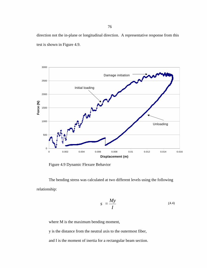
76
direction not the in-plane or longitudinal direction. A representative response from this
test is shown in Figure 4.9.
The bending stress was calculated at two different levels using the following
relationship:
where M is the maximum bending moment,
y is the distance from the neutral axis to the outermost fiber,
and I is the moment of inertia for a rectangular beam section.
I
My=σ (4.4)
Force vs. Displacement for 2-7-tnw-14
0
500
1000
1500
2000
2500
3000
0 0.002 0.004 0.006 0.008 0.01 0.012 0.014 0.016
Displacement (m)
Fo
rce
(N)
Initial loading
Damage initiation
Unloading
Figure 4.9 Dynamic Flexure Behavior

77
The largest force and related stress in the linear range represents the reversible
limit or the stress at which damage initiates. The maximum load and related stress
represent the ultimate limits of the material. The first quantity is the most useful. Ideally
a blade should be able to survive birdstrike and continue operating safely. A blade with
significant damage would not possess the required stiffness and balance for safe
operation.
The energy absorbed was calculated at both the damage initiation and ultimate
load levels. This was done with the following relationship:
where
SE is the Strain energy absorbed by crack growth,
F is the force, xi and xf are initial and final displacements respectively,
and dx is an incremental displacement.
The most pertinent energy absorption metric would be the quantity relating to
the damage initiation level. As with stress, it was considered optimal that an aerofan
blade would sustain the kinetic energy associated with birdstrike and continue to operate.
However some damage tolerance is needed, because a material that promptly detonates
when the reversible limit is exceeded is not desirable.
∫ ⋅=f
i
x
x
dxFSE (4.5)
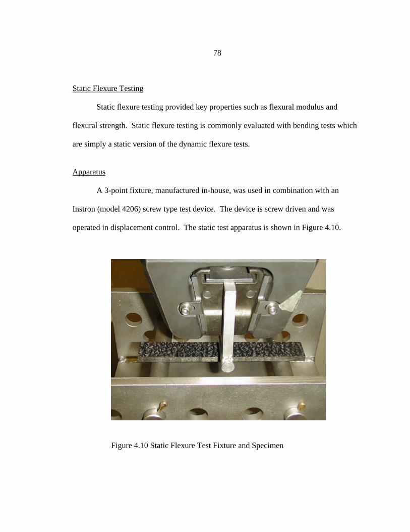
78
Static Flexure Testing
Static flexure testing provided key properties such as flexural modulus and
flexural strength. Static flexure testing is commonly evaluated with bending tests which
are simply a static version of the dynamic flexure tests.
Apparatus
A 3-point fixture, manufactured in-house, was used in combination with an
Instron (model 4206) screw type test device. The device is screw driven and was
operated in displacement control. The static test apparatus is shown in Figure 4.10.
Figure 4.10 Static Flexure Test Fixture and Specimen
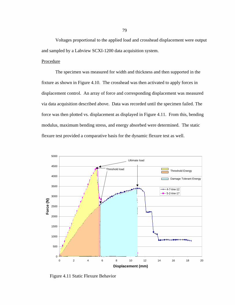
79
Voltages proportional to the applied load and crosshead displacement were output
and sampled by a Labview SCXI-1200 data acquisition system.
Procedure
The specimen was measured for width and thickness and then supported in the
fixture as shown in Figure 4.10. The crosshead was then activated to apply forces in
displacement control. An array of force and corresponding displacement was measured
via data acquisition described above. Data was recorded until the specimen failed. The
force was then plotted vs. displacement as displayed in Figure 4.11. From this, bending
modulus, maximum bending stress, and energy absorbed were determined. The static
flexure test provided a comparative basis for the dynamic flexure test as well.
0
500
1000
1500
2000
2500
3000
3500
4000
4500
5000
0 2 4 6 8 10 12 14 16 18 20
Displacement (mm)
Fo
rce
(N)
4-7-tnw-12
5-2-tnw-17
Threshold load
Ultimate load
Threshold Energy
Damage Tolerant Energy
Figure 4.11 Static Flexure Behavior
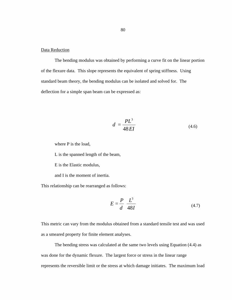
80
Data Reduction
The bending modulus was obtained by performing a curve fit on the linear portion
of the flexure data. This slope represents the equivalent of spring stiffness. Using
standard beam theory, the bending modulus can be isolated and solved for. The
deflection for a simple span beam can be expressed as:
where P is the load,
L is the spanned length of the beam,
E is the Elastic modulus,
and I is the moment of inertia.
This relationship can be rearranged as follows:
This metric can vary from the modulus obtained from a standard tensile test and was used
as a smeared property for finite element analyses.
The bending stress was calculated at the same two levels using Equation (4.4) as
was done for the dynamic flexure. The largest force or stress in the linear range
represents the reversible limit or the stress at which damage initiates. The maximum load
EI
PL
48
3
=δ (4.6)
I
LPE
48
3
⋅=δ (4.7)
81
and related stress represent ultimate limits of the material. Again, the first quantity is the
most useful. While some degree of damage tolerance was desired, resistance to initial
damage was viewed as the primary objective.
Tensile Testing
Several standard tensile test “dog bone” shaped specimens were supplied. These
were subjected to tensile testing to find elastic modulus and ultimate tensile strength.
These properties were not the focus of this investigation, however they were evaluated in
an effort to verify that improvements in durability performance were not causing reduced
strength and stiffness properties.
Apparatus
The Instron (model 4206) screw machine was employed to load the tensile
specimens. Each specimen was equipped with a strain gage, that was incorporated into a
standard Wheatstone bridge circuit with an excitation voltage supplied. Load and
corresponding strain were sampled with a Labview program capable of sampling load
and strain proportional voltage.
Procedure
Specimens were measured for width and thickness at the narrow portion of the
“dog bone” sample. They were then secured into the Instron 4206 by means of the
universal clamp type grips. Load was applied in displacement control. The load and
strain were recorded until the specimen failed. Stress and strain were then plotted to
characterize the tensile characteristics of the material. It should be noted that the strain
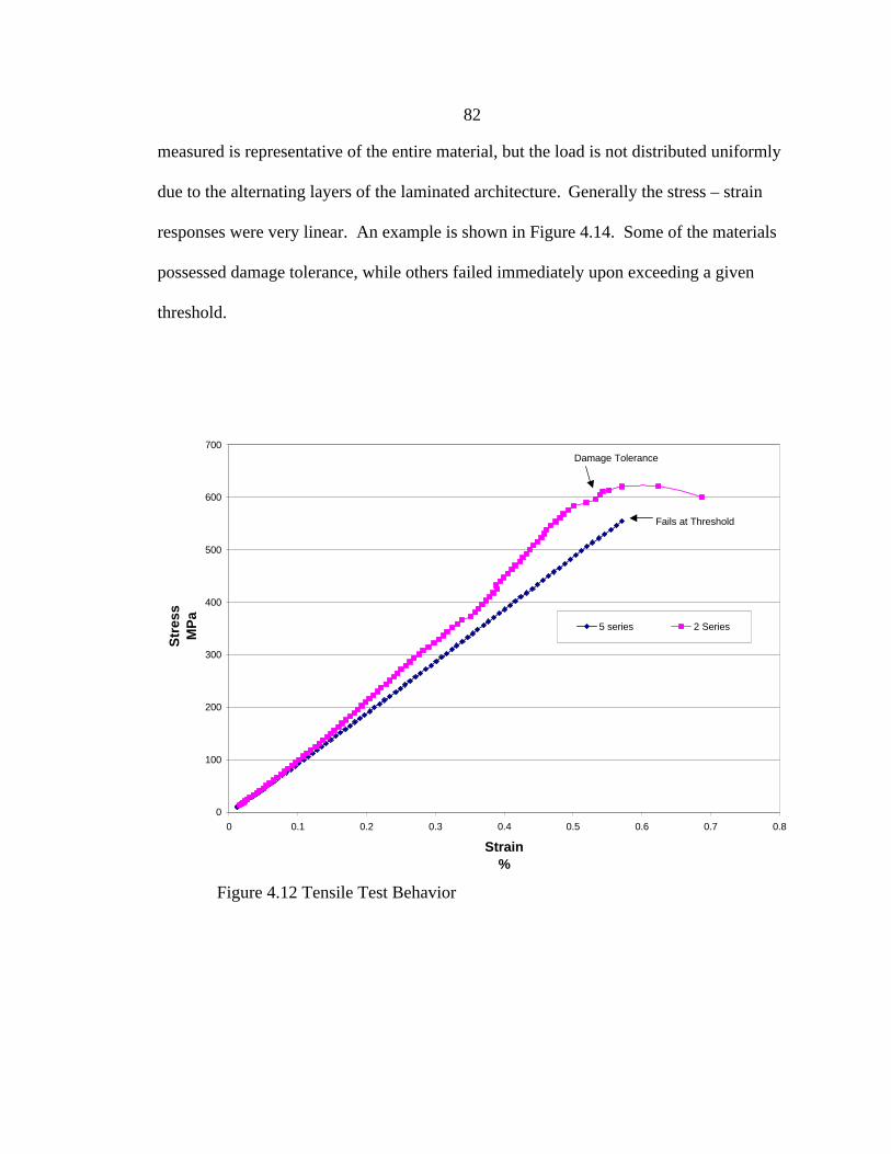
82
measured is representative of the entire material, but the load is not distributed uniformly
due to the alternating layers of the laminated architecture. Generally the stress – strain
responses were very linear. An example is shown in Figure 4.14. Some of the materials
possessed damage tolerance, while others failed immediately upon exceeding a given
threshold.
0
100
200
300
400
500
600
700
0 0.1 0.2 0.3 0.4 0.5 0.6 0.7 0.8
Strain%
Str
ess
MP
a
5 series 2 Series
Damage Tolerance
Fails at Threshold
Figure 4.12 Tensile Test Behavior

83
Experimental Results
Generally, the results obtained are preliminary and do not represent a statistically
significant data set. However based on these results some conclusions can be drawn.
Current results suggest that materials supplied need further development to satisfy the
minimum design requirements for aerofan blades. The 5 series (2-D baseline) composite
showed the most promise in regards to ultimate tensile strength. However, this material
exhibited the worst delamination resistance. Plots comparing all specimen types for each
test conducted are shown in this section. Additionally, a tabular comparison of
preliminary results is included. The results are presented based on tests conducted and
properties evaluated.
Mode II Delamination Resistance Results
Mode II delamination tests were conducted to evaluate GIIc values. Series 1 and 2
under no circumstances would accept a pre-crack. While this indicates very good
delamination resistance, the goal of the test is to measure load and energy required to
propagate an existing crack. The physical inability to initiate a crack made it impossible
to obtain meaningful results from Mode II delamination tests for series 1 and 2 materials.
The 4 series material was pre-cracked, but the crack would not propagate under bending
or shear loading under any circumstances. Only minimal results could be obtained for
this material. Mode II fracture did occur in the 5 series material. Typical fracture
behavior is shown in Figure 4.13 for this material.
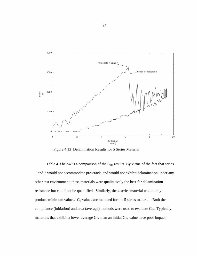
84
Table 4.3 below is a comparison of the GIIc results. By virtue of the fact that series
1 and 2 would not accommodate pre-crack, and would not exhibit delamination under any
other test environment, these materials were qualitatively the best for delamination
resistance but could not be quantified. Similarly, the 4 series material would only
produce minimum values. GII values are included for the 5 series material. Both the
compliance (initiation) and area (average) methods were used to evaluate GIIc. Typically,
materials that exhibit a lower average GIIc than an initial GIIc value have poor impact
0
1000
2000
3000
4000
0 2 4 6 8 10
Crack Propogation
Threshold = 3260 N
Deflection (mm)
For
ce
N
Figure 4.13 Delamination Results for 5 Series Material
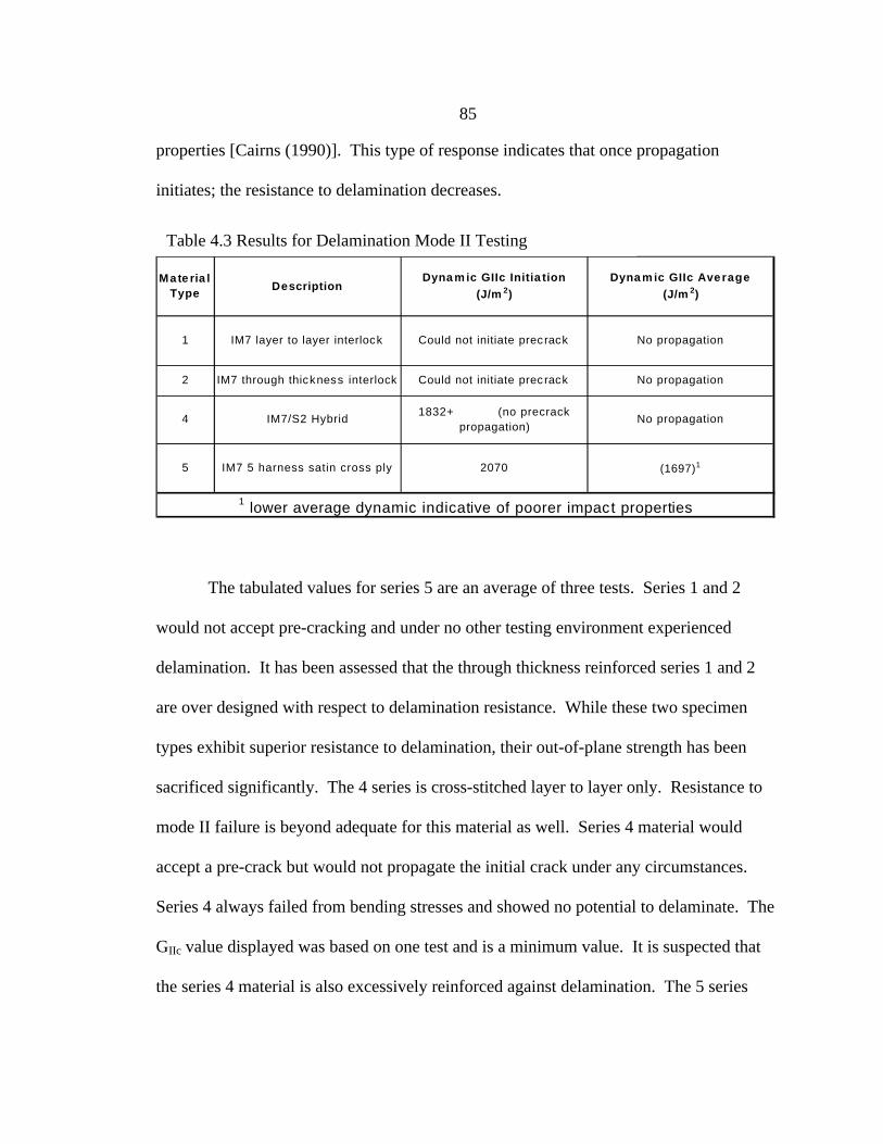
85
properties [Cairns (1990)]. This type of response indicates that once propagation
initiates; the resistance to delamination decreases.
The tabulated values for series 5 are an average of three tests. Series 1 and 2
would not accept pre-cracking and under no other testing environment experienced
delamination. It has been assessed that the through thickness reinforced series 1 and 2
are over designed with respect to delamination resistance. While these two specimen
types exhibit superior resistance to delamination, their out-of-plane strength has been
sacrificed significantly. The 4 series is cross-stitched layer to layer only. Resistance to
mode II failure is beyond adequate for this material as well. Series 4 material would
accept a pre-crack but would not propagate the initial crack under any circumstances.
Series 4 always failed from bending stresses and showed no potential to delaminate. The
GIIc value displayed was based on one test and is a minimum value. It is suspected that
the series 4 material is also excessively reinforced against delamination. The 5 series
Mate ria l Type
DescriptionDyna m ic GIIc Initia tion
(J/m 2)Dyna m ic GIIc Ave rage
(J/m 2)
1 IM7 layer to layer interlock Could not initiate precrack No propagation
2 IM7 through thickness interlock Could not initiate precrack No propagation
4 IM7/S2 Hybrid 1832+ (no precrack
propagation)No propagation
5 IM7 5 harness satin cross ply 2070 (1697)1
1 lower average dynamic indicative of poorer impact properties
Table 4.3 Results for Delamination Mode II Testing
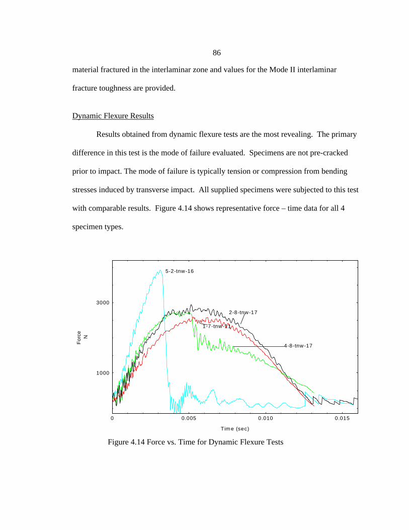
86
material fractured in the interlaminar zone and values for the Mode II interlaminar
fracture toughness are provided.
Dynamic Flexure Results
Results obtained from dynamic flexure tests are the most revealing. The primary
difference in this test is the mode of failure evaluated. Specimens are not pre-cracked
prior to impact. The mode of failure is typically tension or compression from bending
stresses induced by transverse impact. All supplied specimens were subjected to this test
with comparable results. Figure 4.14 shows representative force – time data for all 4
specimen types.
1000
3000
0 0.005 0.010 0.015
5-2-tnw-16
4-8-tnw-17
2-8-tnw-17
1-7-tnw-11
Tim e (sec)
For
ce
N
Figure 4.14 Force vs. Time for Dynamic Flexure Tests
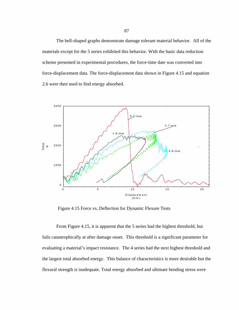
87
The bell-shaped graphs demonstrate damage tolerant material behavior. All of the
materials except for the 5 series exhibited this behavior. With the basic data reduction
scheme presented in experimental procedures, the force-time date was converted into
force-displacement data. The force-displacement data shown in Figure 4.15 and equation
2.6 were then used to find energy absorbed.
From Figure 4.15, it is apparent that the 5 series had the highest threshold, but
fails catastrophically at after damage onset. This threshold is a significant parameter for
evaluating a material’s impact resistance. The 4 series had the next highest threshold and
the largest total absorbed energy. This balance of characteristics is more desirable but the
flexural strength is inadequate. Total energy absorbed and ultimate bending stress were
0
1 0 0 0
2 0 0 0
3 0 0 0
4 0 0 0
0 5 1 0 1 5 2 0
4 -8 -tn w
2 -7 - tn w
5 -2 -tn w
1 -8 -tn w
D is p la c e m e n t(m m )
For
ce
N
Figure 4.15 Force vs. Deflection for Dynamic Flexure Tests
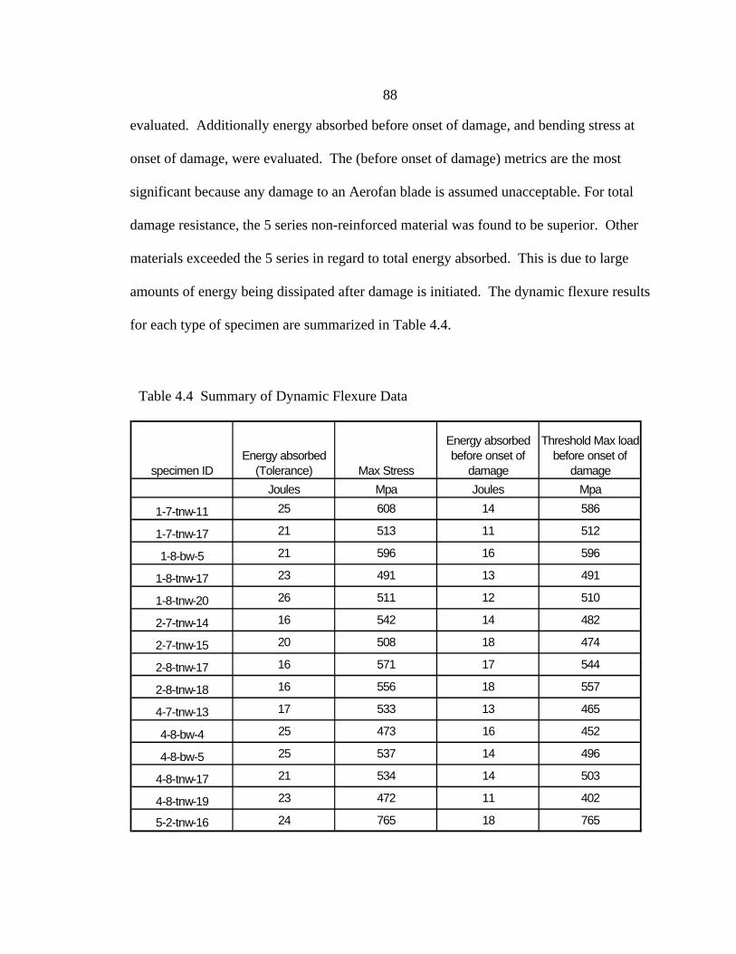
88
evaluated. Additionally energy absorbed before onset of damage, and bending stress at
onset of damage, were evaluated. The (before onset of damage) metrics are the most
significant because any damage to an Aerofan blade is assumed unacceptable. For total
damage resistance, the 5 series non-reinforced material was found to be superior. Other
materials exceeded the 5 series in regard to total energy absorbed. This is due to large
amounts of energy being dissipated after damage is initiated. The dynamic flexure results
for each type of specimen are summarized in Table 4.4.
specimen IDEnergy absorbed
(Tolerance) Max Stress
Energy absorbed before onset of
damage
Threshold Max load before onset of
damage
Joules Mpa Joules Mpa
1-7-tnw-11 25 608 14 586
1-7-tnw-17 21 513 11 512
1-8-bw-5 21 596 16 596
1-8-tnw-17 23 491 13 491
1-8-tnw-20 26 511 12 510
2-7-tnw-14 16 542 14 482
2-7-tnw-15 20 508 18 474
2-8-tnw-17 16 571 17 544
2-8-tnw-18 16 556 18 557
4-7-tnw-13 17 533 13 465
4-8-bw-4 25 473 16 452
4-8-bw-5 25 537 14 496
4-8-tnw-17 21 534 14 503
4-8-tnw-19 23 472 11 402
5-2-tnw-16 24 765 18 765
Table 4.4 Summary of Dynamic Flexure Data
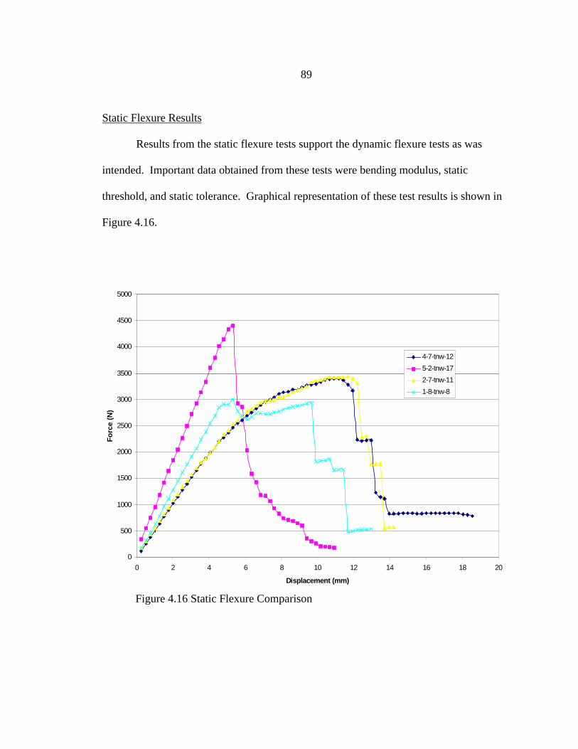
89
Static Flexure Results
Results from the static flexure tests support the dynamic flexure tests as was
intended. Important data obtained from these tests were bending modulus, static
threshold, and static tolerance. Graphical representation of these test results is shown in
Figure 4.16.
0
500
1000
1500
2000
2500
3000
3500
4000
4500
5000
0 2 4 6 8 10 12 14 16 18 20
Displacement (mm)
Fo
rce
(N)
4-7-tnw-12
5-2-tnw-17
2-7-tnw-11
1-8-tnw-8
Figure 4.16 Static Flexure Comparison
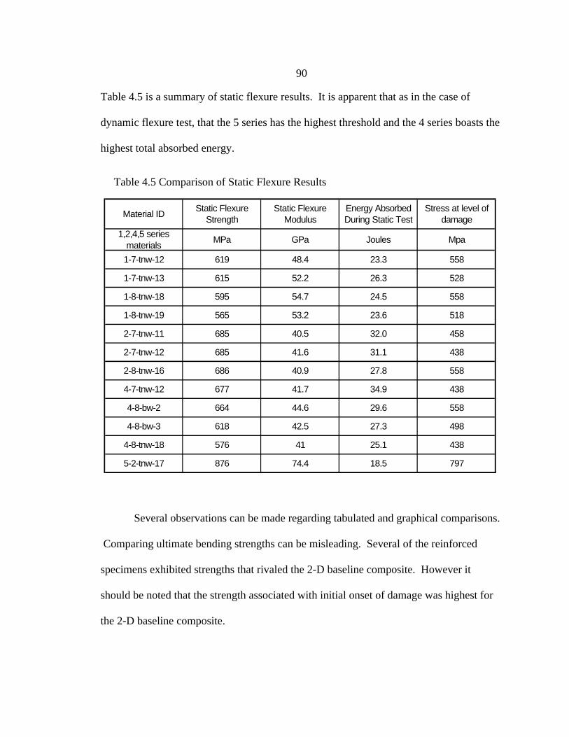
90
Table 4.5 is a summary of static flexure results. It is apparent that as in the case of
dynamic flexure test, that the 5 series has the highest threshold and the 4 series boasts the
highest total absorbed energy.
Several observations can be made regarding tabulated and graphical comparisons.
Comparing ultimate bending strengths can be misleading. Several of the reinforced
specimens exhibited strengths that rivaled the 2-D baseline composite. However it
should be noted that the strength associated with initial onset of damage was highest for
the 2-D baseline composite.
Material IDStatic Flexure
StrengthStatic Flexure
ModulusEnergy Absorbed During Static Test
Stress at level of damage
1,2,4,5 series materials
MPa GPa Joules Mpa
1-7-tnw-12 619 48.4 23.3 558
1-7-tnw-13 615 52.2 26.3 528
1-8-tnw-18 595 54.7 24.5 558
1-8-tnw-19 565 53.2 23.6 518
2-7-tnw-11 685 40.5 32.0 458
2-7-tnw-12 685 41.6 31.1 438
2-8-tnw-16 686 40.9 27.8 558
4-7-tnw-12 677 41.7 34.9 438
4-8-bw-2 664 44.6 29.6 558
4-8-bw-3 618 42.5 27.3 498
4-8-tnw-18 576 41 25.1 438
5-2-tnw-17 876 74.4 18.5 797
Table 4.5 Comparison of Static Flexure Results
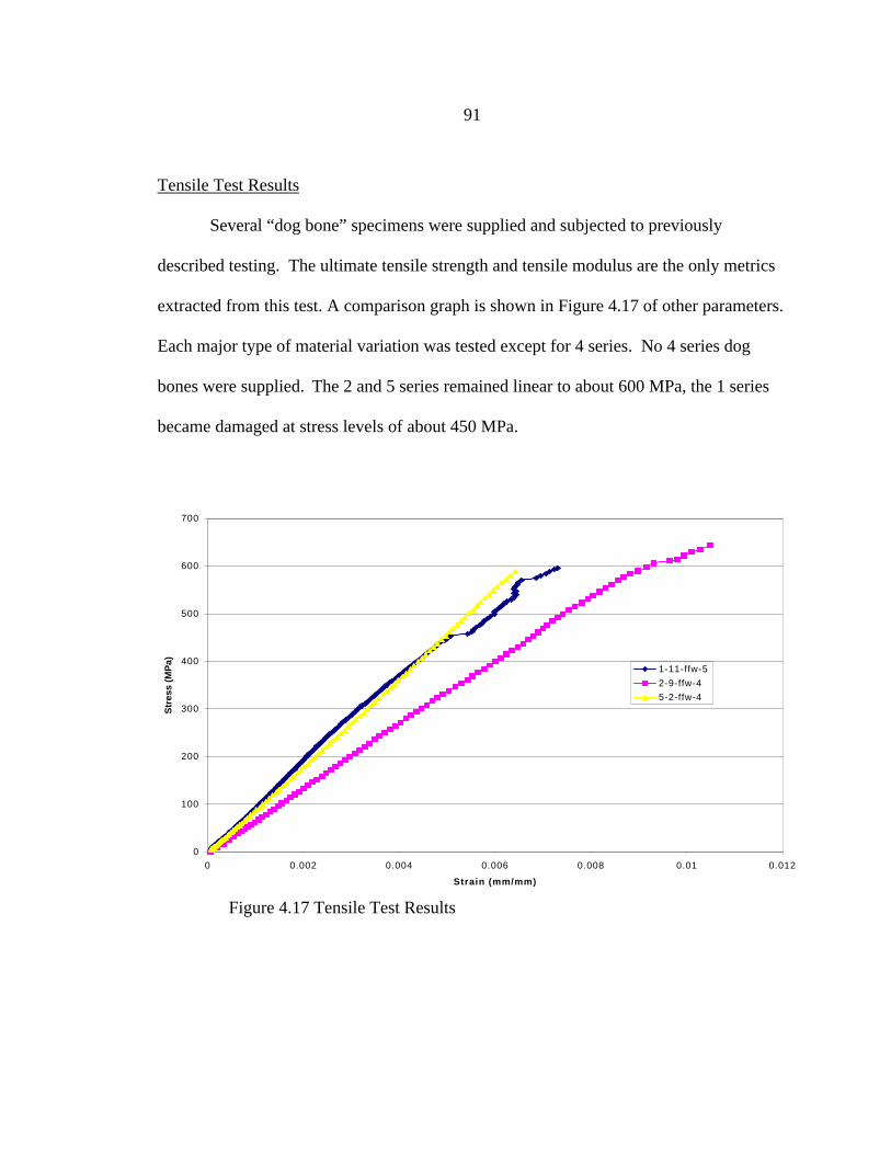
91
Tensile Test Results
Several “dog bone” specimens were supplied and subjected to previously
described testing. The ultimate tensile strength and tensile modulus are the only metrics
extracted from this test. A comparison graph is shown in Figure 4.17 of other parameters.
Each major type of material variation was tested except for 4 series. No 4 series dog
bones were supplied. The 2 and 5 series remained linear to about 600 MPa, the 1 series
became damaged at stress levels of about 450 MPa.
0
100
200
300
400
500
600
700
0 0.002 0.004 0.006 0.008 0.01 0.012
Strain (mm/mm)
Str
ess
(MP
a)
1-11-ffw-5
2-9-ffw-4
5-2-ffw-4
Figure 4.17 Tensile Test Results
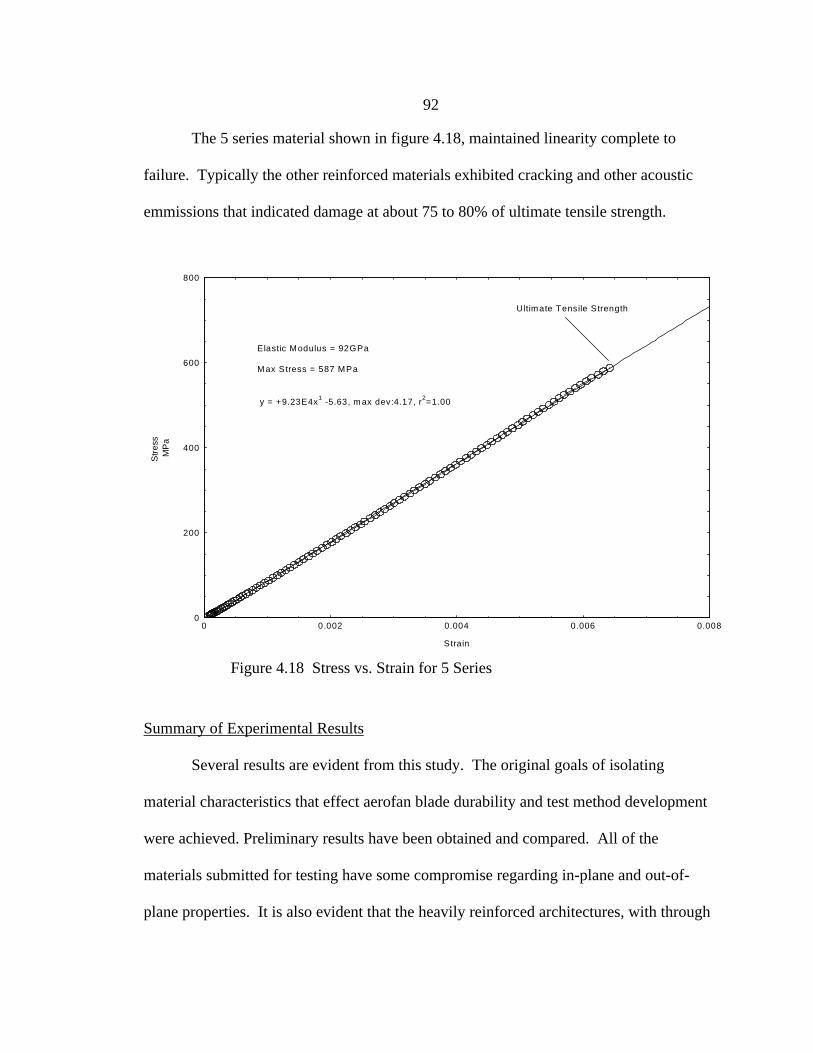
92
The 5 series material shown in figure 4.18, maintained linearity complete to
failure. Typically the other reinforced materials exhibited cracking and other acoustic
emmissions that indicated damage at about 75 to 80% of ultimate tensile strength.
Summary of Experimental Results
Several results are evident from this study. The original goals of isolating
material characteristics that effect aerofan blade durability and test method development
were achieved. Preliminary results have been obtained and compared. All of the
materials submitted for testing have some compromise regarding in-plane and out-of-
plane properties. It is also evident that the heavily reinforced architectures, with through
0
200
400
600
800
0 0.002 0.004 0.006 0.008
Ultimate Tensile Strength
Max Stress = 587 MPa
Elastic Modulus = 92GPa
y = +9.23E4x1 -5.63, m ax dev:4.17, r2=1.00
Strain
Str
ess
MP
a
Figure 4.18 Stress vs. Strain for 5 Series

93
thickness cross-stitching, compromised out of plane strength. Most of the reinforced
materials had larger tolerance or absorbed more total energy than the 2-D version.
However this may be of little use since this energy value and area under the curve
correspond to permanent damage. This justifies the additional calculation of energy
absorbed and other bending strength before the onset of damage. In service it would be
required that a blade withstand an impact and complete the intended flight. Once this
requirement is satisfied, delamination resistance is the next most important consideration
when dealing with composites. Dynamic threshold and delamination requirements must
be met while simultaneously maintaining stiffness, tensile strength and bending strength.
It is additionally necessary to exceed the strength to weight ratio of rival materials such
as titanium before material can be considered a valid candidate.
Suggested material properties are supplied below in Table 4.6. These values are
a blend of properties from the architectures tested in this study. The testing procedures
discussed can be used as a screening process to refine existing material properties.
Table 4.6 Suggested Material Properties for Composite X
Suggested Current best Current best IDDynamic Flex Strength threshold > 800 MPa 765 MPa 5 seriesDynamic GIIc value > 2700 J/m^2 >2700 J/m^2 All but 5 seriesStatic Bending Strength > 850 MPa 797.2 MPa 5 seriesBending Modulus > 69 GPa 74.4 GPa 5 seriesTensile Modulus > 70 GPa > 70 GPa All exceedTensile Strength > 650 MPa 655 MPa 2 seriesStrength to weight ratio undecided not known 5 series
94
Numerical Analysis for Case Study I
Two separate but similar models were developed. One model was meant to
represent flexure testing and the other was designed to simulate ENF or end notch flexure
test. These models were intended to substantiate data reduction techniques used to
calculate material properties such as flexural strength, flexural modulus, and dynamic
mode II fracture toughness. Mode II fracture is generally not as well understood as mode
I. The friction at the sliding interface of the crack could affect the results [Gillespie
(1986)]. Non-conservative values could be produced, by disregarding the friction at the
crack interface.
Static Flexure Approach
From previously conducted static flexure tests the flexure modulus was obtained
experimentally. This modulus was input as a constitutive property in a finite element
model of the specimen tested. This model was then solved for incremental loads up to
the limit of the material. From this, a load – displacement graph could be generated and
compared to the experimental data. Additionally, the bending stress at max load could be
obtained and compared to the bending stress predicted by standard beam formulations.
Static Flexure Model
For the case of the static flexure model a 2-D analysis was conducted. Half
symmetry was employed to reduce the computational burden. A state of plane stress was
assumed and Ansys plane82 elements were used. Typically the mesh consisted of six
elements through the thickness of the modeled static flexure specimen. The aspect ratio
was held to 1x1. The material properties were smeared and obtained from experimental
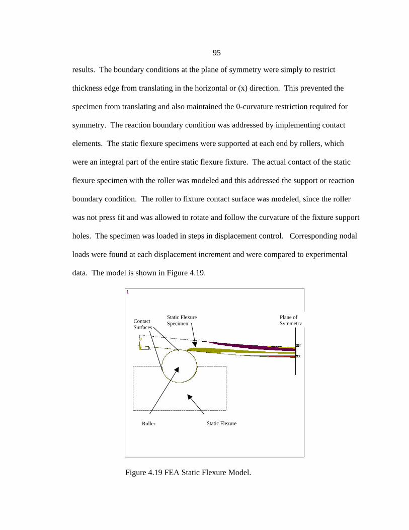
95
results. The boundary conditions at the plane of symmetry were simply to restrict
thickness edge from translating in the horizontal or (x) direction. This prevented the
specimen from translating and also maintained the 0-curvature restriction required for
symmetry. The reaction boundary condition was addressed by implementing contact
elements. The static flexure specimens were supported at each end by rollers, which
were an integral part of the entire static flexure fixture. The actual contact of the static
flexure specimen with the roller was modeled and this addressed the support or reaction
boundary condition. The roller to fixture contact surface was modeled, since the roller
was not press fit and was allowed to rotate and follow the curvature of the fixture support
holes. The specimen was loaded in steps in displacement control. Corresponding nodal
loads were found at each displacement increment and were compared to experimental
data. The model is shown in Figure 4.19.
Static Flexure
Plane ofSymmetry
Roller
Static FlexureSpecimenContact
Surfaces
Figure 4.19 FEA Static Flexure Model.
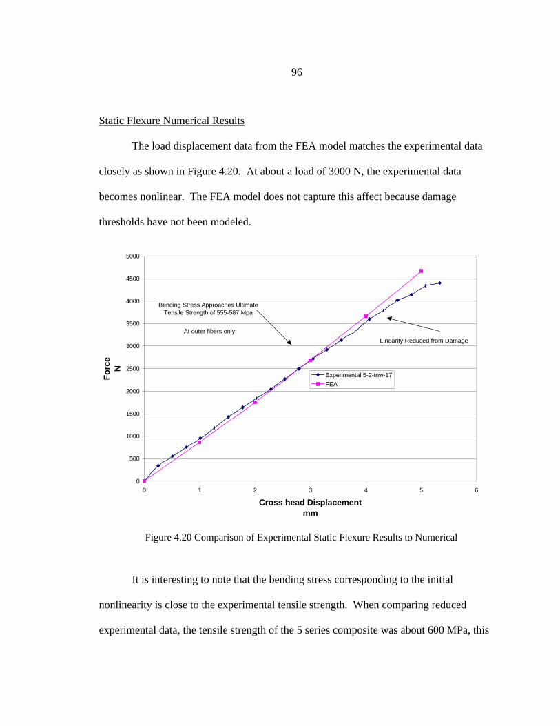
96
Static Flexure Numerical Results
The load displacement data from the FEA model matches the experimental data
closely as shown in Figure 4.20. At about a load of 3000 N, the experimental data
becomes nonlinear. The FEA model does not capture this affect because damage
thresholds have not been modeled.
It is interesting to note that the bending stress corresponding to the initial
nonlinearity is close to the experimental tensile strength. When comparing reduced
experimental data, the tensile strength of the 5 series composite was about 600 MPa, this
0
500
1000
1500
2000
2500
3000
3500
4000
4500
5000
0 1 2 3 4 5 6
Cross head Displacementmm
Fo
rce
N
Experimental 5-2-tnw-17
FEA
Bending Stress Approaches Ultimate Tensile Strength of 555-587 Mpa
At outer fibers only
Linearity Reduced from Damage
Figure 4.20 Comparison of Experimental Static Flexure Results to Numerical
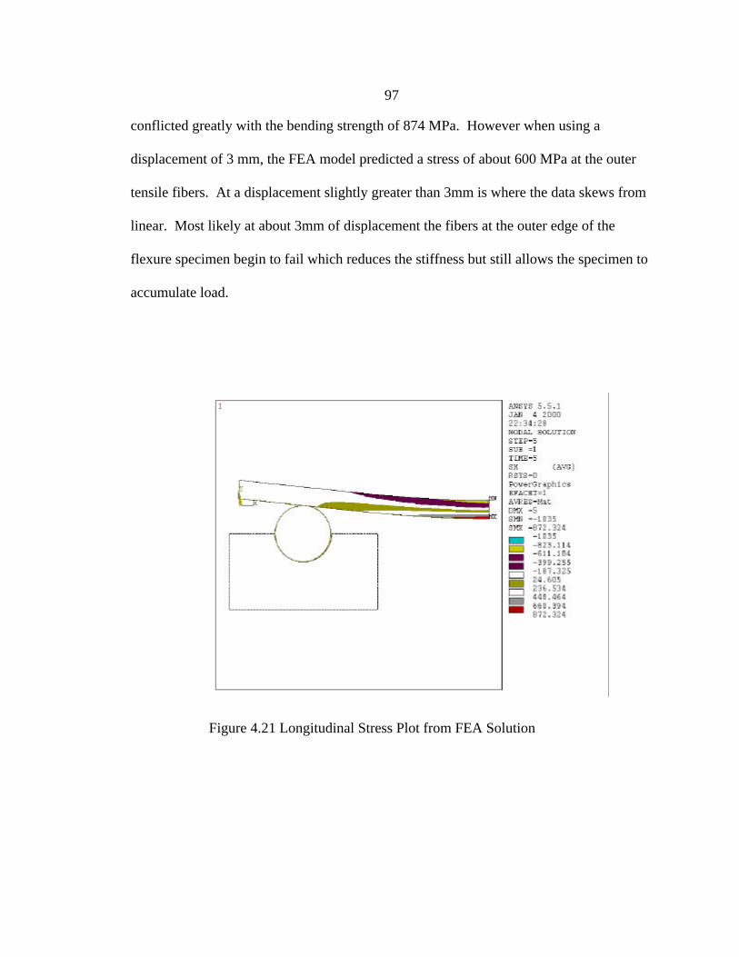
97
conflicted greatly with the bending strength of 874 MPa. However when using a
displacement of 3 mm, the FEA model predicted a stress of about 600 MPa at the outer
tensile fibers. At a displacement slightly greater than 3mm is where the data skews from
linear. Most likely at about 3mm of displacement the fibers at the outer edge of the
flexure specimen begin to fail which reduces the stiffness but still allows the specimen to
accumulate load.
Figure 4.21 Longitudinal Stress Plot from FEA Solution

98
End Notch Flexure Approach
From previously conducted static flexure tests the flexure modulus was obtained
experimentally. This modulus was input as a constitutive property in a finite element
model of an ENF test specimen. Both crack closure techniques and crack extension
methods were used to evaluate Gc numerically. Four solutions were required. Initially
the model was solved with the critical load applied. The total strain energy was output as
well as required nodal data for the single step virtual crack closure technique (VCCT 1).
The model was then resolved with unit loads applied so that relative motion between the
corner nodes immediately behind the crack front would be closed. Nodal displacements
at the corner nodes were output and used with the initial displacements to calculate Gc
(equation 2.10) with the two step method (VCCT 2).
Two crack extension methods were also used. The crack in the original model
was extended by the length of an element. The critical load was held constant and the
model was resolved. The total strain energy was output and used with equation (2.11)
and the original strain energy to calculate Gc. This method is called crack extension 1
(CE 1). A similar technique was applied. Instead of using an incremental extension, the
final crack extension was used from the experimental data. The actual displacement was
applied to the model instead of assuming a constant load. This approach is CE 2.
Friction was accounted for at the crack surface. The validity of the mode II test
has been questioned, mainly due to the effect of friction on these results [Gillespie
(1986)]. This model was evaluated in two steps. Initially the load corresponding to crack
initiation was used with the initial crack length modeled. The model was solved and total
strain energy was output. The model was then resolved in displacement control with the
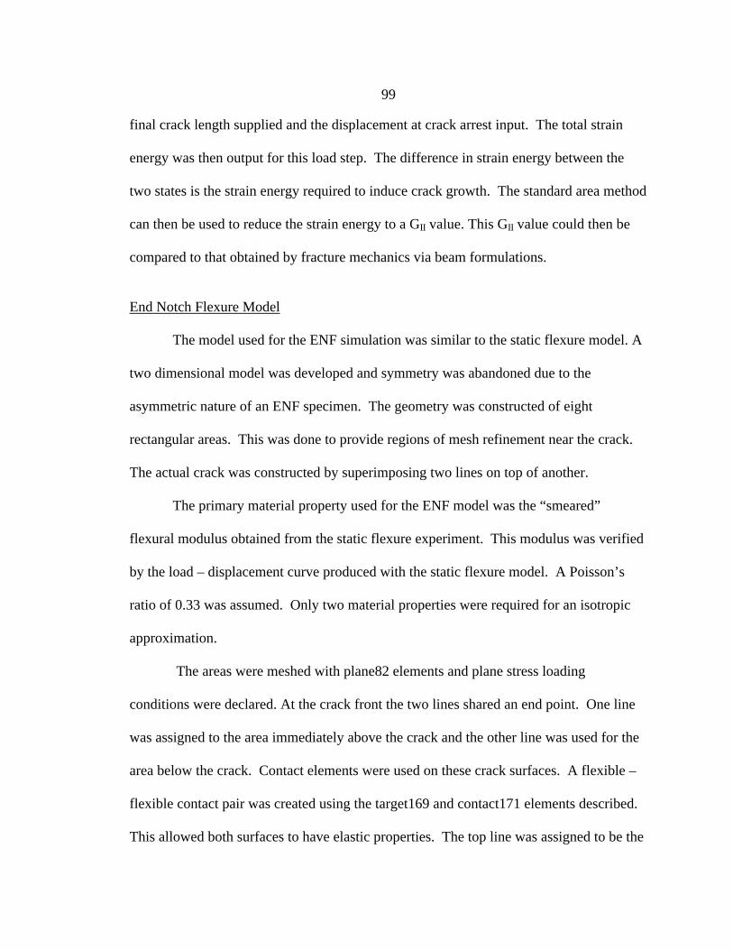
99
final crack length supplied and the displacement at crack arrest input. The total strain
energy was then output for this load step. The difference in strain energy between the
two states is the strain energy required to induce crack growth. The standard area method
can then be used to reduce the strain energy to a GII value. This GII value could then be
compared to that obtained by fracture mechanics via beam formulations.
End Notch Flexure Model
The model used for the ENF simulation was similar to the static flexure model. A
two dimensional model was developed and symmetry was abandoned due to the
asymmetric nature of an ENF specimen. The geometry was constructed of eight
rectangular areas. This was done to provide regions of mesh refinement near the crack.
The actual crack was constructed by superimposing two lines on top of another.
The primary material property used for the ENF model was the “smeared”
flexural modulus obtained from the static flexure experiment. This modulus was verified
by the load – displacement curve produced with the static flexure model. A Poisson’s
ratio of 0.33 was assumed. Only two material properties were required for an isotropic
approximation.
The areas were meshed with plane82 elements and plane stress loading
conditions were declared. At the crack front the two lines shared an end point. One line
was assigned to the area immediately above the crack and the other line was used for the
area below the crack. Contact elements were used on these crack surfaces. A flexible –
flexible contact pair was created using the target169 and contact171 elements described.
This allowed both surfaces to have elastic properties. The top line was assigned to be the
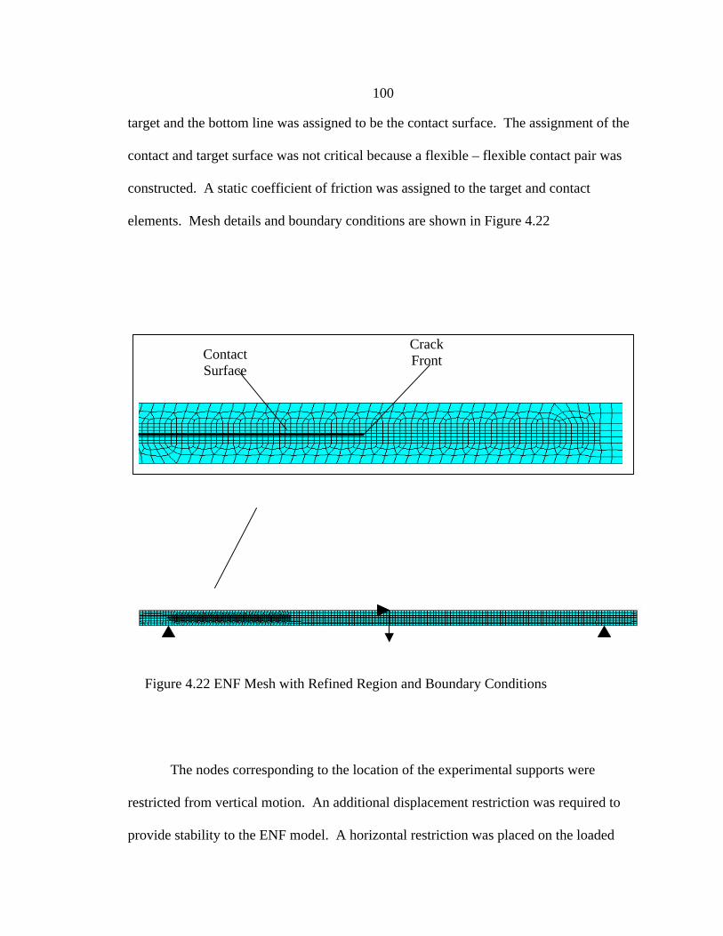
100
target and the bottom line was assigned to be the contact surface. The assignment of the
contact and target surface was not critical because a flexible – flexible contact pair was
constructed. A static coefficient of friction was assigned to the target and contact
elements. Mesh details and boundary conditions are shown in Figure 4.22
The nodes corresponding to the location of the experimental supports were
restricted from vertical motion. An additional displacement restriction was required to
provide stability to the ENF model. A horizontal restriction was placed on the loaded
CrackFrontContact
Surface
Figure 4.22 ENF Mesh with Refined Region and Boundary Conditions
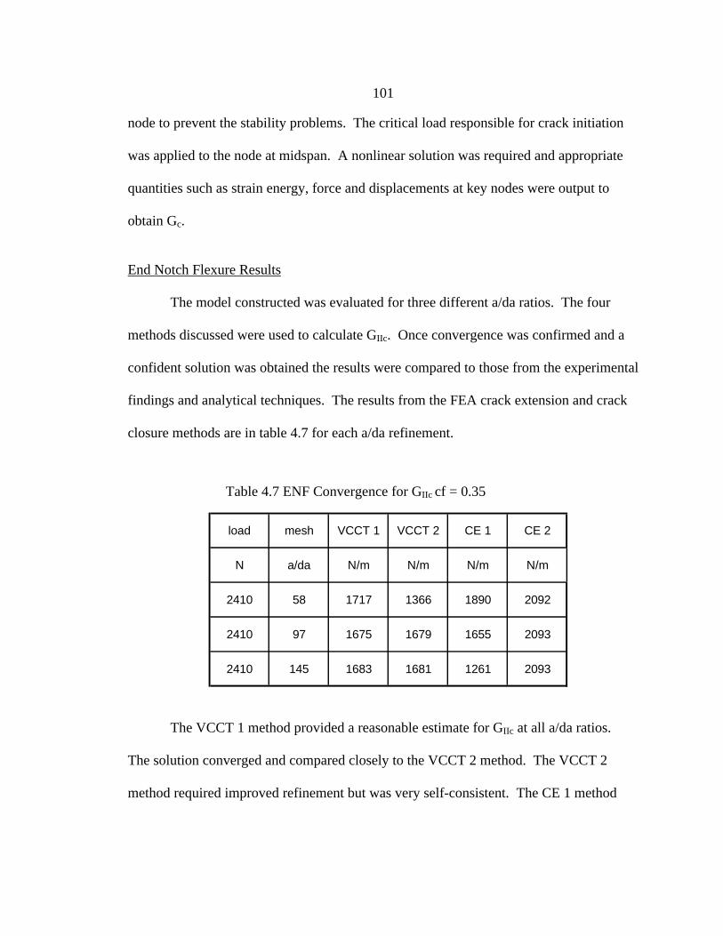
101
node to prevent the stability problems. The critical load responsible for crack initiation
was applied to the node at midspan. A nonlinear solution was required and appropriate
quantities such as strain energy, force and displacements at key nodes were output to
obtain Gc.
End Notch Flexure Results
The model constructed was evaluated for three different a/da ratios. The four
methods discussed were used to calculate GIIc. Once convergence was confirmed and a
confident solution was obtained the results were compared to those from the experimental
findings and analytical techniques. The results from the FEA crack extension and crack
closure methods are in table 4.7 for each a/da refinement.
The VCCT 1 method provided a reasonable estimate for GIIc at all a/da ratios.
The solution converged and compared closely to the VCCT 2 method. The VCCT 2
method required improved refinement but was very self-consistent. The CE 1 method
load mesh VCCT 1 VCCT 2 CE 1 CE 2
N a/da N/m N/m N/m N/m
2410 58 1717 1366 1890 2092
2410 97 1675 1679 1655 2093
2410 145 1683 1681 1261 2093
Table 4.7 ENF Convergence for GIIc cf = 0.35
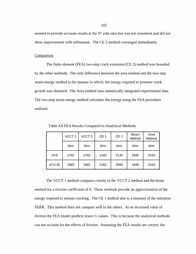
102
seemed to provide accurate results at the 97 a/da ratio but was not consistent and did not
show improvement with refinement. The CE 2 method converged immediately.
Comparison
The finite element (FEA) two-step crack extension (CE 2) method was bounded
by the other methods. The only difference between the area method and the two-step
strain energy method is the manner in which, the energy required to promote crack
growth was obtained. The Area method uses numerically integrated experimental data.
The two-step strain energy method calculates the energy using the FEA procedure
outlined.
The VCCT 1 method compares closely to the VCCT 2 method and the beam
method for a friction coefficient of 0. These methods provide an approximation of the
energy required to initiate cracking. The CE 1 method also is a measure of the initiation
SERR. This method does not compare well to the others. At an increased value of
friction the FEA model predicts lower G values. This is because the analytical methods
can not account for the effects of friction. Assuming the FEA results are correct, the
VCCT 1 VCCT 2 CE 1 CE 2Beam
MethodArea
Method
N/m N/m N/m N/m N/m N/m
cf=0 1791 1791 1182 2130 1845 2163
cf=0.35 1683 1681 1261 2093 1845 2163
Table 4.8 FEA Results Compared to Analytical Methods
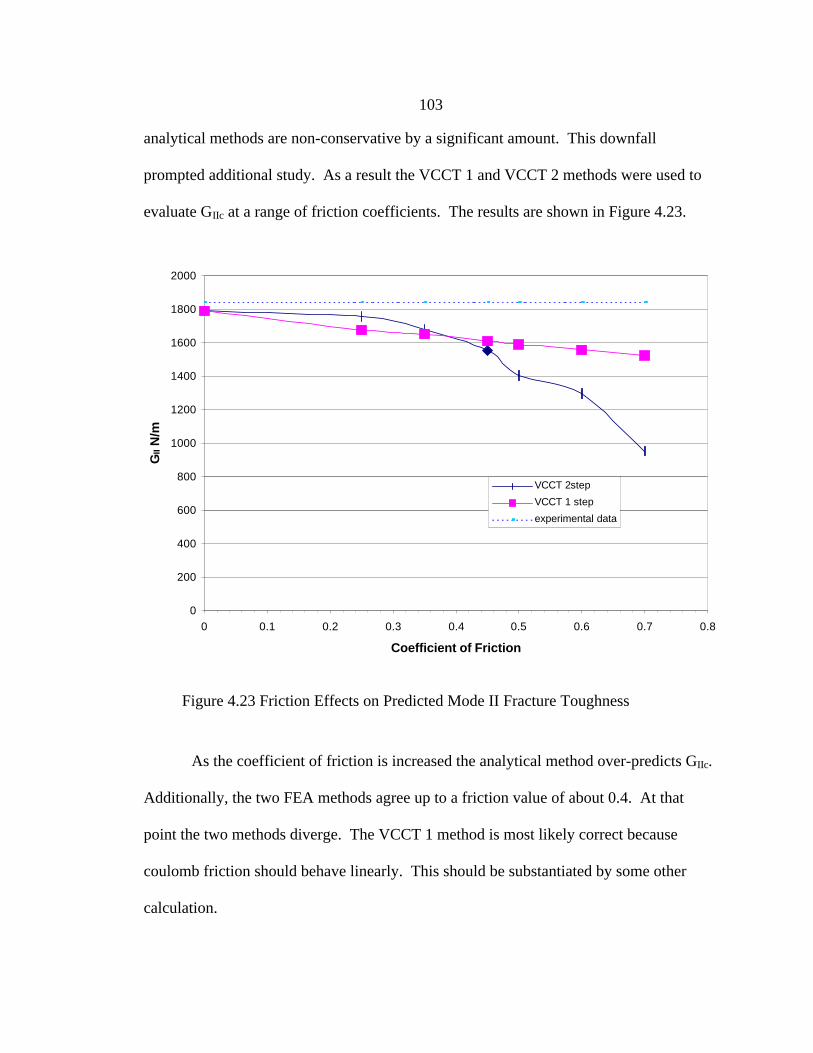
103
analytical methods are non-conservative by a significant amount. This downfall
prompted additional study. As a result the VCCT 1 and VCCT 2 methods were used to
evaluate GIIc at a range of friction coefficients. The results are shown in Figure 4.23.
As the coefficient of friction is increased the analytical method over-predicts GIIc.
Additionally, the two FEA methods agree up to a friction value of about 0.4. At that
point the two methods diverge. The VCCT 1 method is most likely correct because
coulomb friction should behave linearly. This should be substantiated by some other
calculation.
Figure 4.23 Friction Effects on Predicted Mode II Fracture Toughness
0
200
400
600
800
1000
1200
1400
1600
1800
2000
0 0.1 0.2 0.3 0.4 0.5 0.6 0.7 0.8
Coefficient of Friction
GII
N/m
VCCT 2step
VCCT 1 step
experimental data
104
Simple slope tests were conducted to evaluate the friction coefficient between the
two sliding surfaces. The results of these experiments suggest that the friction coefficient
was between 0.45 and 0.55. Based on this approximation the analytical GIIc value was
probably non-conservative by at least 10%. A teflon strip was not used during the
manufacture of the laminates, as a result the crack interface was considerably rough and
consistent with the propagated region.
The Area method and the CE 2 method average the GIIc over a known crack
growth region. These methods account for R-curve behavior and generally predict larger
values for GIIc than the initiation methods.
Test Specimen Validation
The FEA model also provided an immediate inspection tool for stresses. It was
stated earlier that the Area method relates energy absorbed to crack damage. However, if
damage occurs in addition to crack growth, an inflated GII value would result.
The experimental data had two similar test results. These were the 5-tnw-13 and
14 specimens. However the 5-2-tnw-18 specimen varied from these others exceptionally.
The 5-2-tnw-18 specimen possessed a GII value that was twice as much as the others.
This data point indicated that possibly additional damage could have been induced,
beyond crack growth and stimulated further investigation. When consulting with bending
stress and VMS values from the FEA analysis, stress values of 700+ MPa were predicted
for this specimen. These values exceed both the tensile strength and the experimentally
predicted dynamic bending strength. When specimens 13 and 14 were evaluated with the
FEA model, stress levels around 550 to 580 MPa were predicted. This suggests that most

105
likely, specimen 13 and 14 produced reliable GII test results. Possibly a blunt crack was
formed in specimen 18 and before ample energy could be absorbed to initiate crack
growth, parallel modes of failure resulted.
The two-step FEA model was not applied to the other specimens because only the
series 5 material would accept pre-cracking and fail in fracture. However, any additional
material candidates generated (that failed from delamination), could be simulated by this
model.
Summary for Case Study I
In this case study the database-screening approach worked well to isolate key
properties and compare them on a material level. The tests outlined could be used to
evaluate potential composite candidates or refine existing ones. It was noted that
excessive reinforcement through the thickness compromised in plane strength. The
through thickness reinforcement could be optimized to improve fracture toughness
without sacrificing strength. Additionally, the 90 degree fibers could be replaced by 45
degree or 0 degree fabric. This would increase the strength in the primary direction to
compensate for the loss from the addition of the through thickness fibers. This would
allow for increased strength and interlaminar fracture toughness. When converting a
typical stress intensity factor for titanium to a strain energy release rate the Gc for
titanium is 10 times greater than that of the 5 series composite. This suggests that some
through thickness reinforcement is needed to compete with titanium with regards to
toughness. The strength of titanium can be rivaled by making above changes to the
architecture, but only in the primary or longitudinal direction, where needed. The tests

106
provided and methodology presented can be used to optimize and develop composite
candidate materials for this application.
The numerical study focused on evaluating GII for a coupon subjected to flexure.
The analysis used smeared constitutive properties and employed various strain energy
approaches to evaluate G. From the work completed it was found that the crack closure
methods work and compare well to the analytical equation for GIIc. The crack closure
methods can also account for friction at the crack interface. When including friction on
the crack interface in the models, it was found that both the VCCT 1 method and the
VCCT 2 method agreed well for friction coefficients below 0.3. At friction values above
0.3 the G values diverged and from each other, as well as from the analytical equation
which does not address friction effects. A two-step crack extension method was also
applied that included friction affects. This method was compared to the energy method,
which averages G over some distance of crack growth. The two-step strain energy
method compared well with the experimental area method, which indicates that not
accounting for friction when applying the area method is actually less errant than when
using the compliance method. The primary revelation from this study is that the
analytical method used to quantify GII over-predicts the fracture toughness. Models like
the ones presented should be used to isolate GII from experimental tests and the friction
should be included in any model where discrete crack damage modeling is taking place.
The VCCT 1 method was easiest to use and provided reasonable results through a range
of friction coefficients.
Overall the database-screening approach proved sufficient to compare composite
material candidates on a qualitative and quantitative level. Design drivers or key
107
properties were isolated and appropriate tests were formulated to determine these
properties. Once obtained, the experimental properties were compared. The tests
outlined could be used determine material limitations and assist in improving them. The
experiments conducted are part of a general methodology formulated to evaluate
interlaminar fracture performance.
When investigating the database – prediction approach it was found that when
attempting to model mode II fracture behavior, friction needs to be accounted for. Some
sort of friction knock-down factor should be used for the original GII obtained from
experiments, or an FEA model should be employed to evaluate the actual GII.
108
CHAPTER 5
CASE STUDY IIHONEYCOMB FUEL TANK INVESTIGATION
This project employed a database – screening approach as in case study I. Basic
material properties were identified that related to structural performance. Experimental
procedures were developed to test these properties. These materials were then compared
as a screening process to find the limiting source of performance for the honeycomb
composite material. Both interlaminar fracture and strength properties were evaluated.
Additionally, some advancement was made regarding analytical modeling.
Flatwise tension models were used to confirm validity of experimental procedures. Mode
I simulations were developed to substantiate experimental findings and to validate a
compliance equation derived for sandwich panel GI testing. Mode II models were also
developed to confirm experimental technique and interpret results.
Project Introduction
The X-33 was the most recent generation of spacecraft. A significant effort was
made to reduce the weight of the fuel cells, which contain liquid helium and liquid
hydrogen. The solution was to make the fuel cells from a honeycomb type sandwich
panel. These honeycomb fuel tanks were originally constructed full scale and little was
known about the properties of the honeycomb sandwich material.
A catastrophic failure occurred during bond processing of Lobe 1 of Tank-1 of the
X33 liquid hydrogen tank assembly [HPC (2000)]. Many curing stages are necessary for
final assembly, and failure occurred during Cure 4a. On January 13 and 14, 1999, the
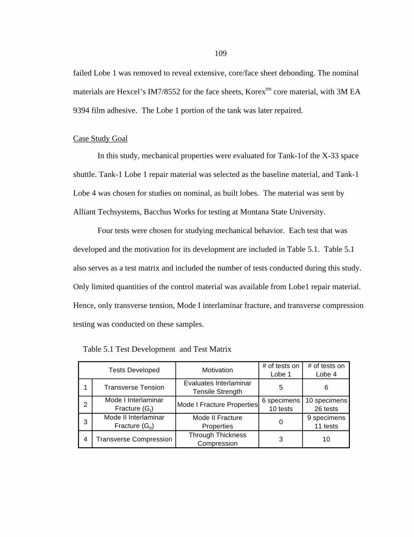
109
failed Lobe 1 was removed to reveal extensive, core/face sheet debonding. The nominal
materials are Hexcel’s IM7/8552 for the face sheets, Korextm core material, with 3M EA
9394 film adhesive. The Lobe 1 portion of the tank was later repaired.
Case Study Goal
In this study, mechanical properties were evaluated for Tank-1of the X-33 space
shuttle. Tank-1 Lobe 1 repair material was selected as the baseline material, and Tank-1
Lobe 4 was chosen for studies on nominal, as built lobes. The material was sent by
Alliant Techsystems, Bacchus Works for testing at Montana State University.
Four tests were chosen for studying mechanical behavior. Each test that was
developed and the motivation for its development are included in Table 5.1. Table 5.1
also serves as a test matrix and included the number of tests conducted during this study.
Only limited quantities of the control material was available from Lobe1 repair material.
Hence, only transverse tension, Mode I interlaminar fracture, and transverse compression
testing was conducted on these samples.
Tests Developed Motivation# of tests on
Lobe 1# of tests on
Lobe 4
1 Transverse TensionEvaluates Interlaminar
Tensile Strength5 6
2Mode I Interlaminar
Fracture (GI)Mode I Fracture Properties
6 specimens 10 tests
10 specimens 26 tests
3Mode II Interlaminar
Fracture (GII)Mode II Fracture
Properties0
9 specimens 11 tests
4 Transverse CompressionThrough Thickness
Compression3 10
Table 5.1 Test Development and Test Matrix
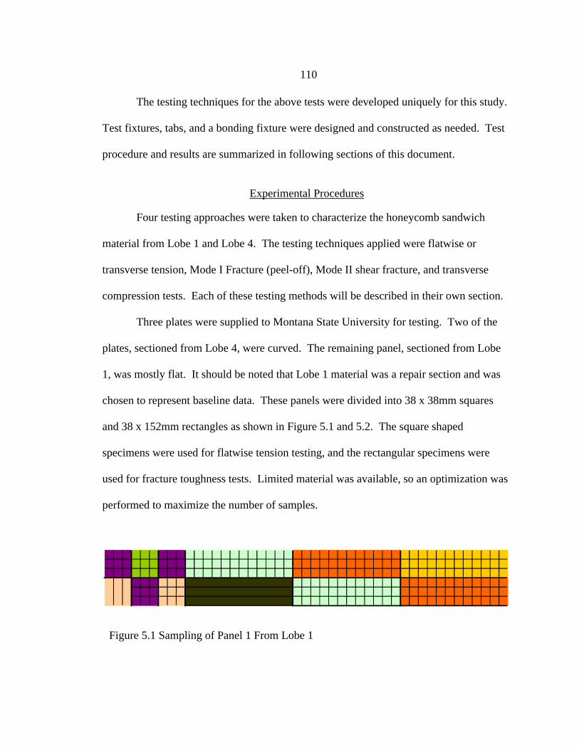
110
The testing techniques for the above tests were developed uniquely for this study.
Test fixtures, tabs, and a bonding fixture were designed and constructed as needed. Test
procedure and results are summarized in following sections of this document.
Experimental Procedures
Four testing approaches were taken to characterize the honeycomb sandwich
material from Lobe 1 and Lobe 4. The testing techniques applied were flatwise or
transverse tension, Mode I Fracture (peel-off), Mode II shear fracture, and transverse
compression tests. Each of these testing methods will be described in their own section.
Three plates were supplied to Montana State University for testing. Two of the
plates, sectioned from Lobe 4, were curved. The remaining panel, sectioned from Lobe
1, was mostly flat. It should be noted that Lobe 1 material was a repair section and was
chosen to represent baseline data. These panels were divided into 38 x 38mm squares
and 38 x 152mm rectangles as shown in Figure 5.1 and 5.2. The square shaped
specimens were used for flatwise tension testing, and the rectangular specimens were
used for fracture toughness tests. Limited material was available, so an optimization was
performed to maximize the number of samples.
Figure 5.1 Sampling of Panel 1 From Lobe 1
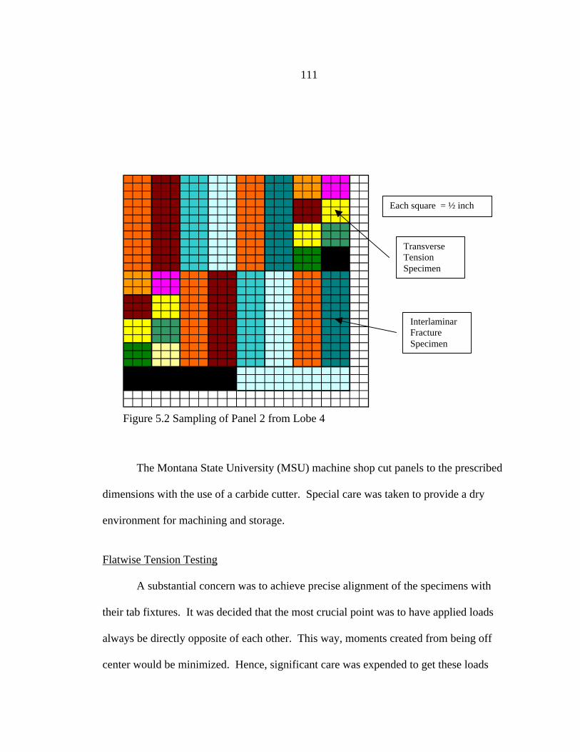
111
The Montana State University (MSU) machine shop cut panels to the prescribed
dimensions with the use of a carbide cutter. Special care was taken to provide a dry
environment for machining and storage.
Flatwise Tension Testing
A substantial concern was to achieve precise alignment of the specimens with
their tab fixtures. It was decided that the most crucial point was to have applied loads
always be directly opposite of each other. This way, moments created from being off
center would be minimized. Hence, significant care was expended to get these loads
Figure 5.2 Sampling of Panel 2 from Lobe 4
Each square = ½ inch
TransverseTensionSpecimen
InterlaminarFractureSpecimen
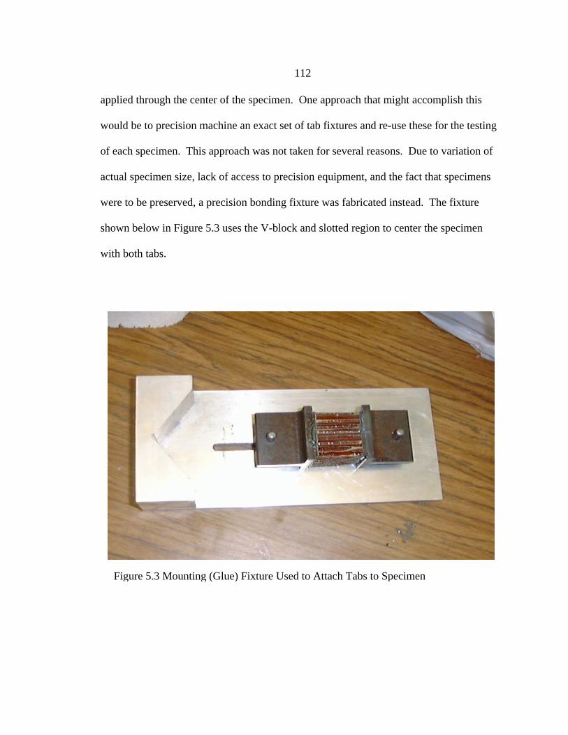
112
applied through the center of the specimen. One approach that might accomplish this
would be to precision machine an exact set of tab fixtures and re-use these for the testing
of each specimen. This approach was not taken for several reasons. Due to variation of
actual specimen size, lack of access to precision equipment, and the fact that specimens
were to be preserved, a precision bonding fixture was fabricated instead. The fixture
shown below in Figure 5.3 uses the V-block and slotted region to center the specimen
with both tabs.
Figure 5.3 Mounting (Glue) Fixture Used to Attach Tabs to Specimen

113
The specimen was glued to top tab first using the V block and slot. Then the
partially glued assembly was slid upward and the bottom tab was attached with aid of an
alignment pin. This aligned the holes of each fixture with the center of the specimen.
This system can be used with a range of specimen sizes and tab dimensions. This
allowed the tab fixtures to be mass-produced and attached in a precise and accurate
fashion. The specimens could then be glued and oven cured at 65 degrees Celsius. This
was done in batches of about four.
Specimen Preparation
Approximately 6 specimens were tested from each lobe. The 38 x 38mm square
specimens were pulled apart in the direction transverse to the face sheet layers. This was
accomplished by attaching fabricated tabs to the top and bottom of the specimens. The
fixtures were simply pieces of steel T-section crosscut to at least 38mm. The tabs were
very stiff to preclude any distortion during testing. These T-sections were then fitted
with a 6mm hole through the web. The tabs were held to the specimen by means of
various glues. The most common adhesive used was Hysol.EA 9309.2NA QT System.
This two-part epoxy had excellent bond strength of about 27 MPa, but was difficult to
work with. Other epoxies used were over the counter glues made by Devcon. These
were easier to apply but did not always have the strength of Hysol. A specimen ready to
be aligned and tested is shown in Figure 5.4.
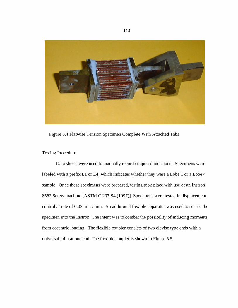
114
Testing Procedure
Data sheets were used to manually record coupon dimensions. Specimens were
labeled with a prefix L1 or L4, which indicates whether they were a Lobe 1 or a Lobe 4
sample. Once these specimens were prepared, testing took place with use of an Instron
8562 Screw machine [ASTM C 297-94 (1997)]. Specimens were tested in displacement
control at rate of 0.08 mm / min. An additional flexible apparatus was used to secure the
specimen into the Instron. The intent was to combat the possibility of inducing moments
from eccentric loading. The flexible coupler consists of two clevise type ends with a
universal joint at one end. The flexible coupler is shown in Figure 5.5.
Figure 5.4 Flatwise Tension Specimen Complete With Attached Tabs
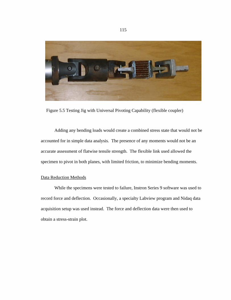
115
Adding any bending loads would create a combined stress state that would not be
accounted for in simple data analysis. The presence of any moments would not be an
accurate assessment of flatwise tensile strength. The flexible link used allowed the
specimen to pivot in both planes, with limited friction, to minimize bending moments.
Data Reduction Methods
While the specimens were tested to failure, Instron Series 9 software was used to
record force and deflection. Occasionally, a specialty Labview program and Nidaq data
acquisition setup was used instead. The force and deflection data were then used to
obtain a stress-strain plot.
Figure 5.5 Testing Jig with Universal Pivoting Capability (flexible coupler)

116
Stress was represented as:
where P was the recorded force in Newtons,
and A was the overall cross sectional area.
Strain was determined as:
where δ was the crosshead displacement,
and L was the core thickness.
The ultimate tensile strength the value of the largest load seen by material divided by the
cross-sectional area. It should be again noted that the cross-sectional area was based on
the outermost dimensions, not actual core paper area. The “effective” elastic modulus
was found from linear regression and was based on the assumption that all of the
displacement read corresponded to the extension of the paper core. The strain at failure
was evaluated based on cross-head displacement measurements. All of these values are
labeled on each individual graph. A sample graphical representation is shown in Figure
5.6. All tests conducted were later compiled and compared on a tabular basis. Statistical
A
P=σ (5.1)
L
δε = (5.2)
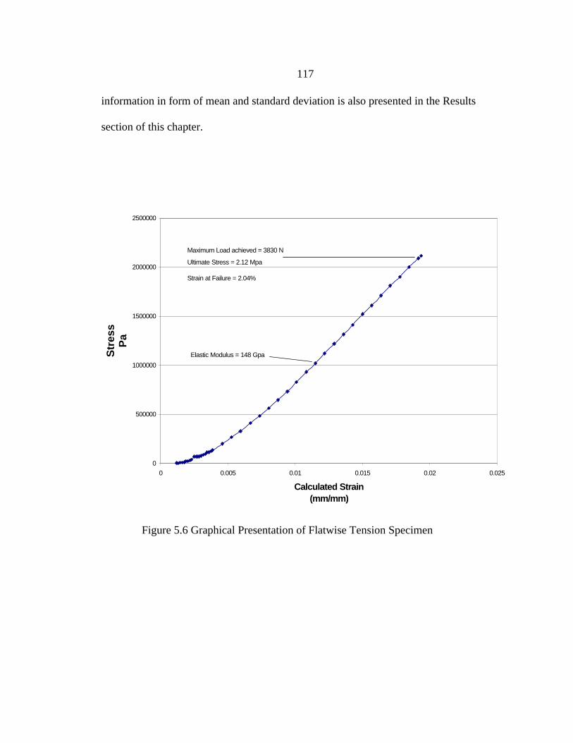
117
information in form of mean and standard deviation is also presented in the Results
section of this chapter.
Figure 5.6 Graphical Presentation of Flatwise Tension Specimen
0
500000
1000000
1500000
2000000
2500000
0 0.005 0.01 0.015 0.02 0.025
Calculated Strain(mm/mm)
Str
ess
Pa
Maximum Load achieved = 3830 N
Ultimate Stress = 2.12 Mpa
Elastic Modulus = 148 Gpa
Strain at Failure = 2.04%
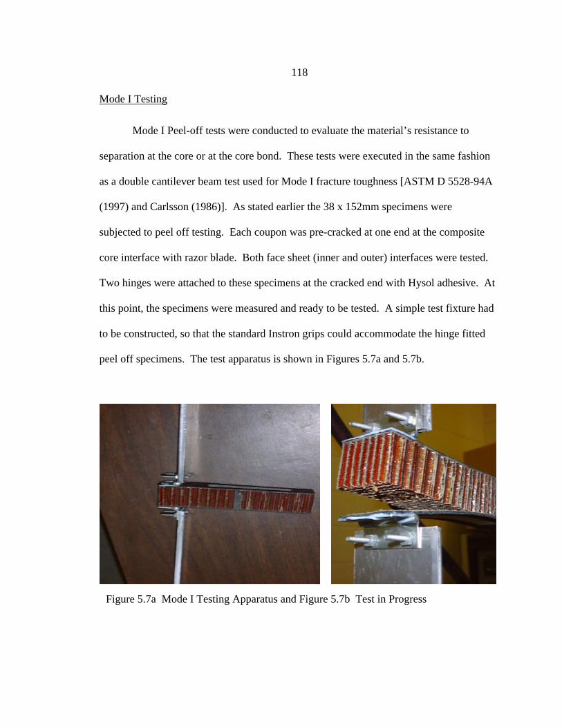
118
Mode I Testing
Mode I Peel-off tests were conducted to evaluate the material’s resistance to
separation at the core or at the core bond. These tests were executed in the same fashion
as a double cantilever beam test used for Mode I fracture toughness [ASTM D 5528-94A
(1997) and Carlsson (1986)]. As stated earlier the 38 x 152mm specimens were
subjected to peel off testing. Each coupon was pre-cracked at one end at the composite
core interface with razor blade. Both face sheet (inner and outer) interfaces were tested.
Two hinges were attached to these specimens at the cracked end with Hysol adhesive. At
this point, the specimens were measured and ready to be tested. A simple test fixture had
to be constructed, so that the standard Instron grips could accommodate the hinge fitted
peel off specimens. The test apparatus is shown in Figures 5.7a and 5.7b.
Figure 5.7a Mode I Testing Apparatus and Figure 5.7b Test in Progress
119
Testing Procedure
Force and deflection were obtained via Labview data acquisition. Initial and final
crack lengths were measured by means of visual inspection with the use of 4 digit-
precision calipers. Each specimen was initially given a pre-crack of about 40mm. Forces
were applied, in displacement control at 0.025 mm/sec until the crack propagated
approximately one inch. The peel-off specimen was then unloaded to obtain a complete
hysteresis. Once the specimen was completely relaxed and the final crack measured, the
test was repeated until crack extended past the mid-plane of the sample. Testing would
be stopped and crack growth or new crack length was measured. This was repeated up to
three times for each specimen. The panels presented to MSU for testing had face sheets
of varying thickness. Tests were conducted with the initial crack on the thin side as well
as the thick side.
Data Reduction Methods
Ultimately, some measure of peel off resistance was desired. The approach taken
to achieve this was an energy method. The force deflection data was integrated resulting
in total energy absorbed for each crack session. This total energy was then divided by the
specimen width multiplied by crack length (eq2.2). The result was the Mode I critical
strain energy release rate [Broek (1996) and ASTM D 5528-94A (1997)].
Since each specimen was subjected to repeated crack growth, 3 to 4 GI values
were obtained for each rectangular specimen. Usually, the first GI values obtained were
larger than subsequent values. The information from the first test was probably not valid
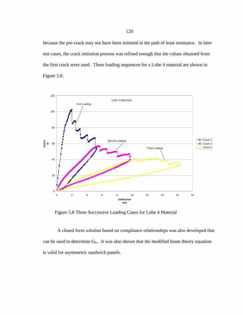
120
because the pre-crack may not have been initiated in the path of least resistance. In later
test cases, the crack initiation process was refined enough that the values obtained from
the first crack were used. Three loading sequences for a Lobe 4 material are shown in
Figure 5.8.
A closed form solution based on compliance relationships was also developed that
can be used to determine GIc. It was also shown that the modified beam theory equation
is valid for asymmetric sandwich panels.
0
20
40
60
80
100
120
0 2 4 6 8 10 12 14 16 18
Deflectionmm
Fo
rce
N
Crack 1
Crack 2
Crack 3
First Loading
Second Loading
Third Loading
Lobe 4 Specimen
Figure 5.8 Three Successive Loading Cases for Lobe 4 Material

121
Mode II Testing
In addition to Mode I type peel testing and flatwise tensile testing, Mode II type
fracture evaluation was also desired. The main difference in this mode of crack
propagation is the driving force. Mode I crack propagation is a function of direct
separation of the face sheet from the core material. Mode II crack propagation is a result
of shear stresses, and was induced from bending. As a result, the testing configuration
varies. Mode II tests were conducted in three point bending fashion. Two rollers provide
support while a loading nose provides the driving force to induce in plane fracture
[Carlsson (1986) and Carlsson (1991)]. The actual testing fixture and machine used are
shown in Figure 5.9. Loading tabs were used to distribute loading and reaction forces.
When this was not done, compression crushing of core material was experienced.
Figure 5.9 Mode II Testing Apparatus In Progress
122
Testing Procedure
The specimens were loaded in a 3 point bending configuration at a rate of about
0.8 mm/minute. Load and cross-head displacement were sampled by means of Labview
data acquisition. When sharp cracking was heard, or when the load suddenly decreased,
the specimen was unloaded. Testing in this fashion allowed hysteretic behavior to be
captured. Crack growth was measured by means of visual inspection and calipers.
Repeat testing was rarely made on mode II specimens. The crack typically propagated to
at least the mid-span, and only core crushing would result from further testing. For valid
GII tests, crack propagation must be the primary failure mode. If various modes of failure
are present, then the energy measured corresponds to crushing, crack propagation, and
bending failure.
Data Reduction Methods
Data reduction for Mode II tests are the same as for Mode I. A variety of beam-
theory type equations exist [Cairns (1992) and Carlsson (1991)]. However, these usually
apply to a material with a crack in the center. The area method described before was
used instead. The area method is dependable as long as the damage region is known.
The graphical output differs from Mode I and is illustrated in Figure 5.10. The sharp drop
shown above was a result of a sudden increase in compliance, as a consequence of crack
growth. Hysteresis was not always captured for the Mode II tests. The specimen would
begin to load after the crack has propagated and arrested. This occurred because the
specimen was tested in displacement control. These data points were disregarded
because they were not related to crack growth.
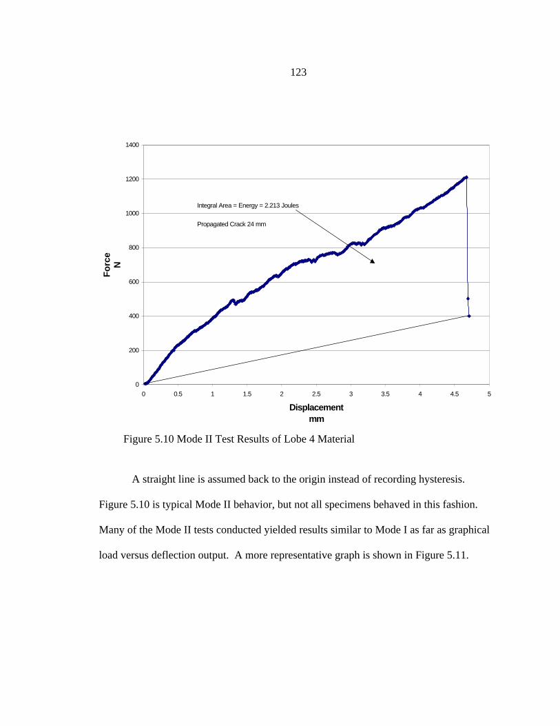
123
A straight line is assumed back to the origin instead of recording hysteresis.
Figure 5.10 is typical Mode II behavior, but not all specimens behaved in this fashion.
Many of the Mode II tests conducted yielded results similar to Mode I as far as graphical
load versus deflection output. A more representative graph is shown in Figure 5.11.
0
200
400
600
800
1000
1200
1400
0 0.5 1 1.5 2 2.5 3 3.5 4 4.5 5
Displacementmm
Fo
rce
N
Integral Area = Energy = 2.213 Joules
Propagated Crack 24 mm
Figure 5.10 Mode II Test Results of Lobe 4 Material
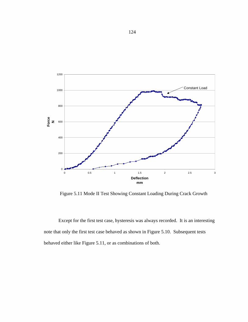
124
Except for the first test case, hysteresis was always recorded. It is an interesting
note that only the first test case behaved as shown in Figure 5.10. Subsequent tests
behaved either like Figure 5.11, or as combinations of both.
0
200
400
600
800
1000
1200
0 0.5 1 1.5 2 2.5 3
Deflectionmm
Fo
rce
N
Constant Load
Figure 5.11 Mode II Test Showing Constant Loading During Crack GrowthPropagation
125
Flatwise Compression Testing
Flatwise compression tests were also conducted on recycled specimens [ASTM C
365-94 (1997)]. Usually, the Mode I specimens would have about 50mm of virgin
material left after three to four crack propagations. Due to excess bending of the face
sheets only four cracks could be obtained for the Mode I specimens. The remaining
untested material was sectioned from the Mode I specimens and used for compression
testing. This testing was not originally requested, however, compressive strength and
compressive modulus can be relevant properties [Astrom (1997)] depending on applied
stresses.
Specimen Preparation
The compression specimens were cut to approximately 38 x 38mm squares. This
size was chosen because these dimensions were used for flatwise tension. Additionally,
these dimensions were the largest that would fit the compression fixtures of the Instron
4206. Once salvaged, they were then simply labeled and measured. They were carefully
inspected to insure that no prior damage existed.
Testing Procedure
Special testing fixtures were used with the Instron 4206 machine for flatwise
compression. Load and Displacement were sampled at a test rate of about 1.0
mm/minute. Testing was conducted in displacement control until the load peaked and the
specimen collapsed. All data were recorded using Labview data acquisition. A
representative graph of the test apparatus is shown in Figure 5.12.
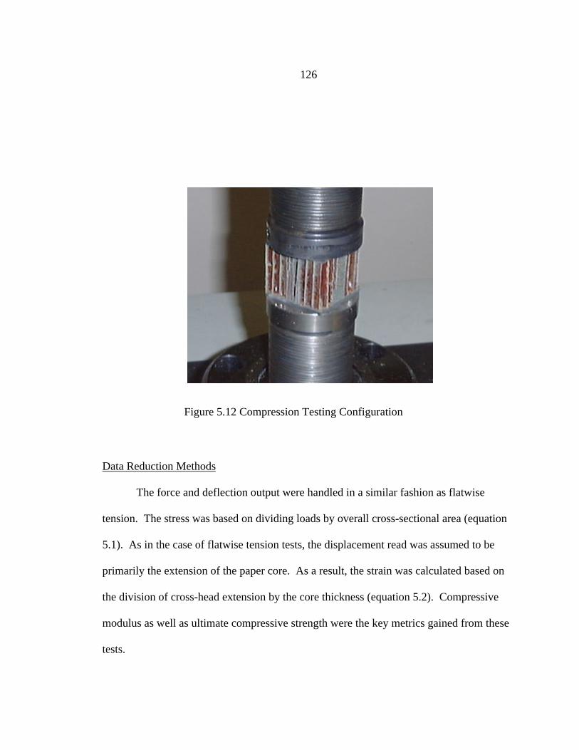
126
Data Reduction Methods
The force and deflection output were handled in a similar fashion as flatwise
tension. The stress was based on dividing loads by overall cross-sectional area (equation
5.1). As in the case of flatwise tension tests, the displacement read was assumed to be
primarily the extension of the paper core. As a result, the strain was calculated based on
the division of cross-head extension by the core thickness (equation 5.2). Compressive
modulus as well as ultimate compressive strength were the key metrics gained from these
tests.
Figure 5.12 Compression Testing Configuration
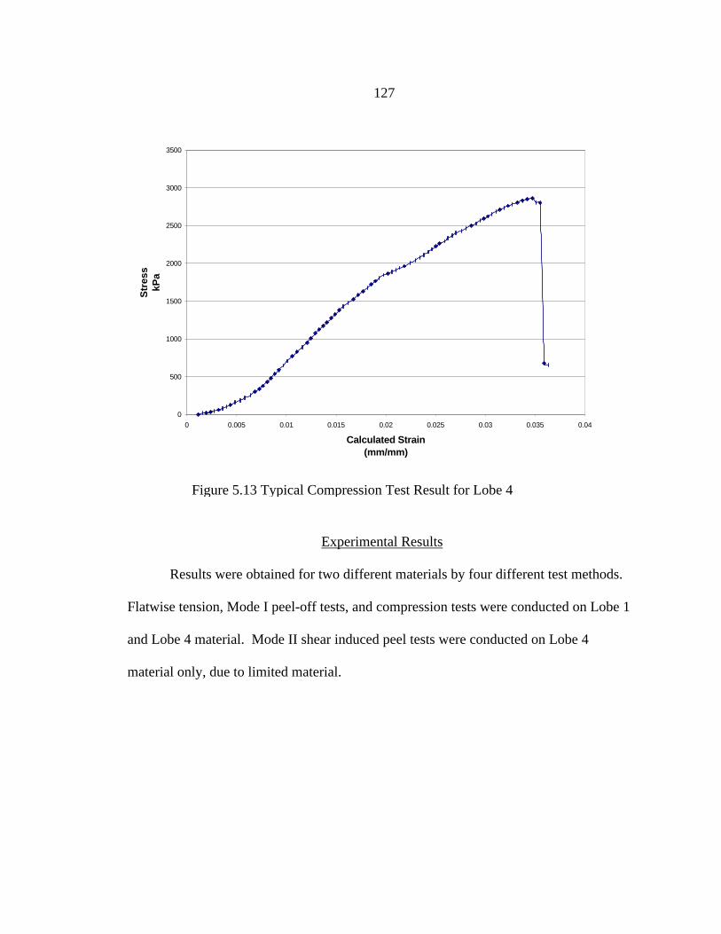
127
Experimental Results
Results were obtained for two different materials by four different test methods.
Flatwise tension, Mode I peel-off tests, and compression tests were conducted on Lobe 1
and Lobe 4 material. Mode II shear induced peel tests were conducted on Lobe 4
material only, due to limited material.
0
500
1000
1500
2000
2500
3000
3500
0 0.005 0.01 0.015 0.02 0.025 0.03 0.035 0.04
Calculated Strain(mm/mm)
Str
ess
kPa
Figure 5.13 Typical Compression Test Result for Lobe 4
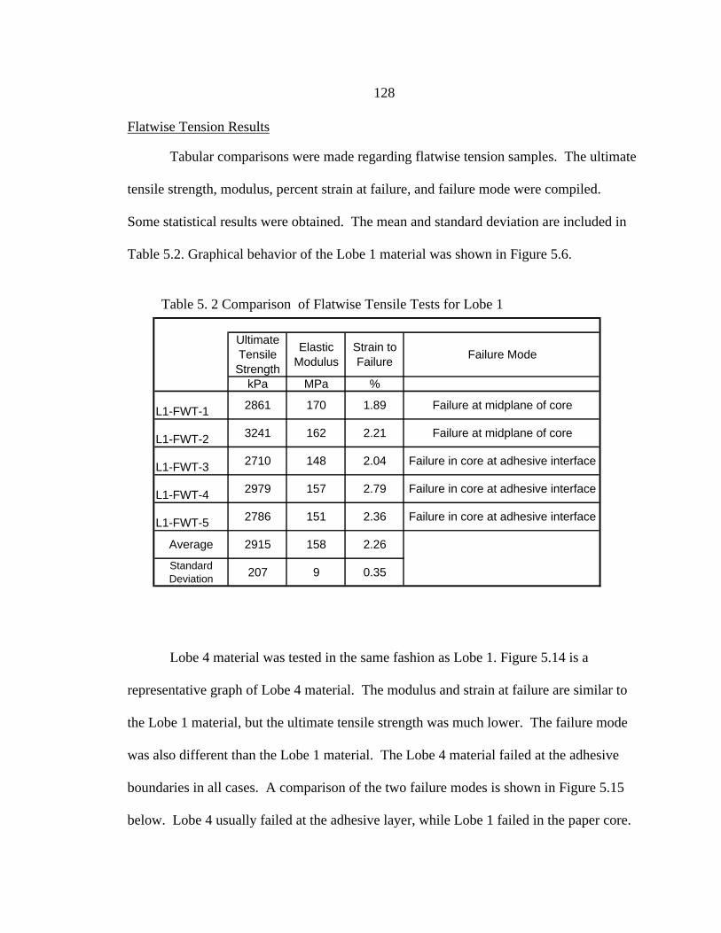
128
Flatwise Tension Results
Tabular comparisons were made regarding flatwise tension samples. The ultimate
tensile strength, modulus, percent strain at failure, and failure mode were compiled.
Some statistical results were obtained. The mean and standard deviation are included in
Table 5.2. Graphical behavior of the Lobe 1 material was shown in Figure 5.6.
Lobe 4 material was tested in the same fashion as Lobe 1. Figure 5.14 is a
representative graph of Lobe 4 material. The modulus and strain at failure are similar to
the Lobe 1 material, but the ultimate tensile strength was much lower. The failure mode
was also different than the Lobe 1 material. The Lobe 4 material failed at the adhesive
boundaries in all cases. A comparison of the two failure modes is shown in Figure 5.15
below. Lobe 4 usually failed at the adhesive layer, while Lobe 1 failed in the paper core.
Table 5. 2 Comparison of Flatwise Tensile Tests for Lobe 1
Ultimate Tensile Strength
Elastic Modulus
Strain to Failure
Failure Mode
kPa MPa %
L1-FWT-1 2861 170 1.89 Failure at midplane of core
L1-FWT-2 3241 162 2.21 Failure at midplane of core
L1-FWT-3 2710 148 2.04 Failure in core at adhesive interface
L1-FWT-4 2979 157 2.79 Failure in core at adhesive interface
L1-FWT-5 2786 151 2.36 Failure in core at adhesive interface
Average 2915 158 2.26
Standard Deviation
207 9 0.35
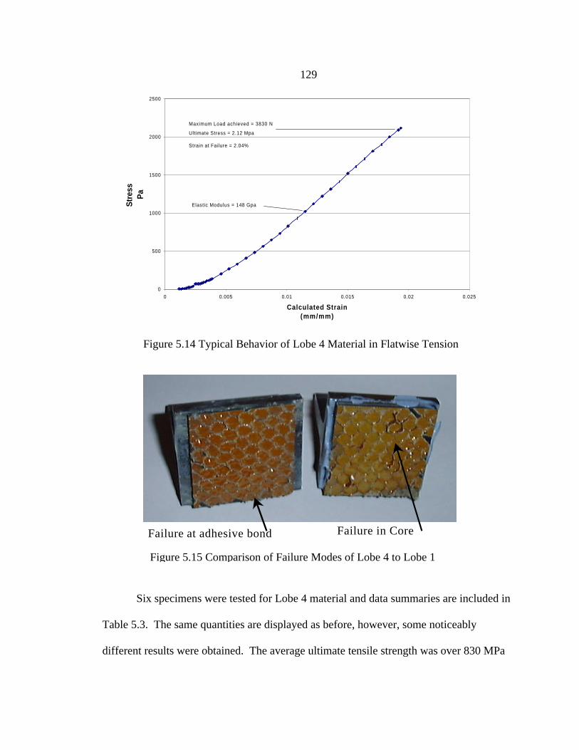
129
Six specimens were tested for Lobe 4 material and data summaries are included in
Table 5.3. The same quantities are displayed as before, however, some noticeably
different results were obtained. The average ultimate tensile strength was over 830 MPa
Failure in Core Failure at adhesive bond
Figure 5.15 Comparison of Failure Modes of Lobe 4 to Lobe 1
Figure 5.14 Graphical Presentation of Flat-wise Tension Specimen L4-FWT-3-
0
500
1000
1500
2000
2500
0 0.005 0.01 0.015 0.02 0.025
Calculated Strain(mm/mm)
Str
ess
Pa
Maximum Load achieved = 3830 N
Ultimate Stress = 2.12 Mpa
Elastic Modulus = 148 Gpa
Strain at Failure = 2.04%
Figure 5.14 Typical Behavior of Lobe 4 Material in Flatwise Tension
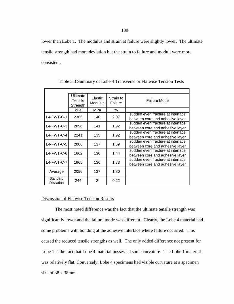
130
lower than Lobe 1. The modulus and strain at failure were slightly lower. The ultimate
tensile strength had more deviation but the strain to failure and moduli were more
consistent.
Discussion of Flatwise Tension Results
The most noted difference was the fact that the ultimate tensile strength was
significantly lower and the failure mode was different. Clearly, the Lobe 4 material had
some problems with bonding at the adhesive interface where failure occurred. This
caused the reduced tensile strengths as well. The only added difference not present for
Lobe 1 is the fact that Lobe 4 material possessed some curvature. The Lobe 1 material
was relatively flat. Conversely, Lobe 4 specimens had visible curvature at a specimen
size of 38 x 38mm.
Table 5.3 Summary of Lobe 4 Transverse or Flatwise Tension Tests
Ultimate Tensile Strength
Elastic Modulus
Strain to Failure
Failure Mode
kPa MPa %
L4-FWT-C-1 2365 140 2.07sudden even fracture at interface between core and adhesive layer
L4-FWT-C-3 2096 141 1.92sudden even fracture at interface between core and adhesive layer
L4-FWT-C-4 2241 135 1.92sudden even fracture at interface between core and adhesive layer
L4-FWT-C-5 2006 137 1.69sudden even fracture at interface between core and adhesive layer
L4-FWT-C-6 1662 136 1.44sudden even fracture at interface between core and adhesive layer
L4-FWT-C-7 1965 136 1.73sudden even fracture at interface between core and adhesive layer
Average 2056 137 1.80
Standard Deviation
244 2 0.22
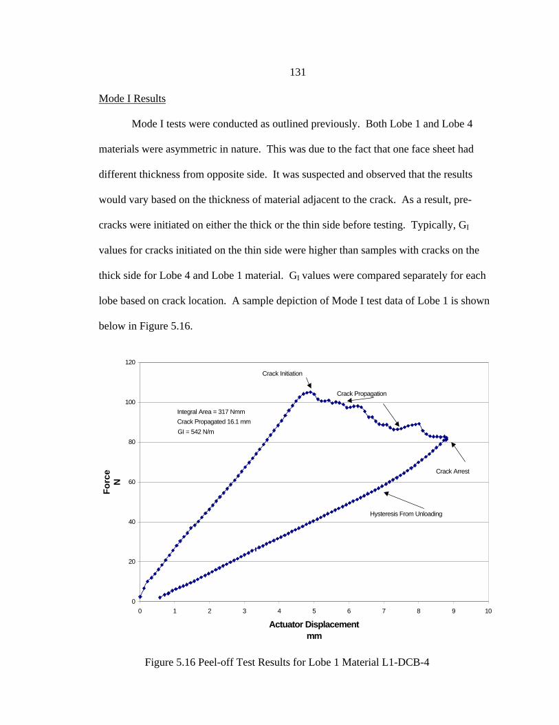
131
Mode I Results
Mode I tests were conducted as outlined previously. Both Lobe 1 and Lobe 4
materials were asymmetric in nature. This was due to the fact that one face sheet had
different thickness from opposite side. It was suspected and observed that the results
would vary based on the thickness of material adjacent to the crack. As a result, pre-
cracks were initiated on either the thick or the thin side before testing. Typically, GI
values for cracks initiated on the thin side were higher than samples with cracks on the
thick side for Lobe 4 and Lobe 1 material. GI values were compared separately for each
lobe based on crack location. A sample depiction of Mode I test data of Lobe 1 is shown
below in Figure 5.16.
0
20
40
60
80
100
120
0 1 2 3 4 5 6 7 8 9 10
Actuator Displacementmm
Fo
rce
N
Integral Area = 317 Nmm
Crack Initiation
Crack Propagation
Crack Arrest
Crack Propagated 16.1 mm
GI = 542 N/m
Hysteresis From Unloading
Figure 5.16 Peel-off Test Results for Lobe 1 Material L1-DCB-42nCrack.

132
The results above are from a test where the crack was initiated on the thin side.
These results are from the propagation of the second crack. Typically, the data from the
first crack propagation was thought to be non-conservative. The initial crack medium
was most likely a more tortuous path than what would be typical. However, all
subsequent cracks were assumed to follow the path that provided the least crack
resistance. The secondary cracks are more likely to possess a more realistic crack tip, as
opposed to the initial pre-crack. All data for each crack session were recorded but some
crack 1 data were not included in average. The variance of the data was reduced when
these values were discarded. The data also maintained its identity regarding whether the
crack was initiated on the thin side or the thick side. Energy absorbed, initial crack
length, final crack length, and GI values are displayed in Table 5.4. Average GI and
standard deviation for both crack conditions are tabulated as well.
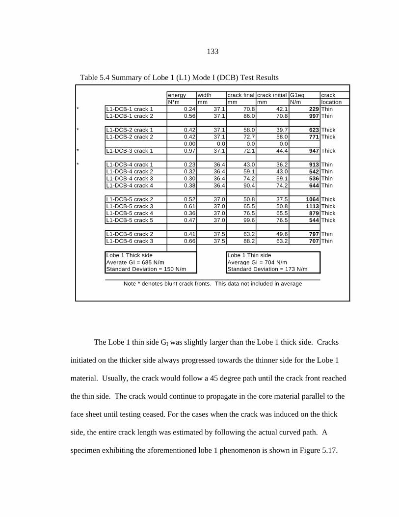
133
The Lobe 1 thin side GI was slightly larger than the Lobe 1 thick side. Cracks
initiated on the thicker side always progressed towards the thinner side for the Lobe 1
material. Usually, the crack would follow a 45 degree path until the crack front reached
the thin side. The crack would continue to propagate in the core material parallel to the
face sheet until testing ceased. For the cases when the crack was induced on the thick
side, the entire crack length was estimated by following the actual curved path. A
specimen exhibiting the aforementioned lobe 1 phenomenon is shown in Figure 5.17.
energy width crack final crack initial G1eq crack N*m mm mm mm N/m location
* L1-DCB-1 crack 1 0.24 37.1 70.8 42.1 229 ThinL1-DCB-1 crack 2 0.56 37.1 86.0 70.8 997 Thin
* L1-DCB-2 crack 1 0.42 37.1 58.0 39.7 623 ThickL1-DCB-2 crack 2 0.42 37.1 72.7 58.0 771 Thick
0.00 0.0 0.0 0.0* L1-DCB-3 crack 1 0.97 37.1 72.1 44.4 947 Thick
* L1-DCB-4 crack 1 0.23 36.4 43.0 36.2 913 ThinL1-DCB-4 crack 2 0.32 36.4 59.1 43.0 542 ThinL1-DCB-4 crack 3 0.30 36.4 74.2 59.1 536 ThinL1-DCB-4 crack 4 0.38 36.4 90.4 74.2 644 Thin
L1-DCB-5 crack 2 0.52 37.0 50.8 37.5 1064 ThickL1-DCB-5 crack 3 0.61 37.0 65.5 50.8 1113 ThickL1-DCB-5 crack 4 0.36 37.0 76.5 65.5 879 ThickL1-DCB-5 crack 5 0.47 37.0 99.6 76.5 544 Thick
L1-DCB-6 crack 2 0.41 37.5 63.2 49.6 797 ThinL1-DCB-6 crack 3 0.66 37.5 88.2 63.2 707 Thin
Lobe 1 Thick side Lobe 1 Thin side
Standard Deviation = 150 N/m Standard Deviation = 173 N/mAverate GI = 685 N/m Average GI = 704 N/m
Note * denotes blunt crack fronts. This data not included in average
Table 5.4 Summary of Lobe 1 (L1) Mode I (DCB) Test Results
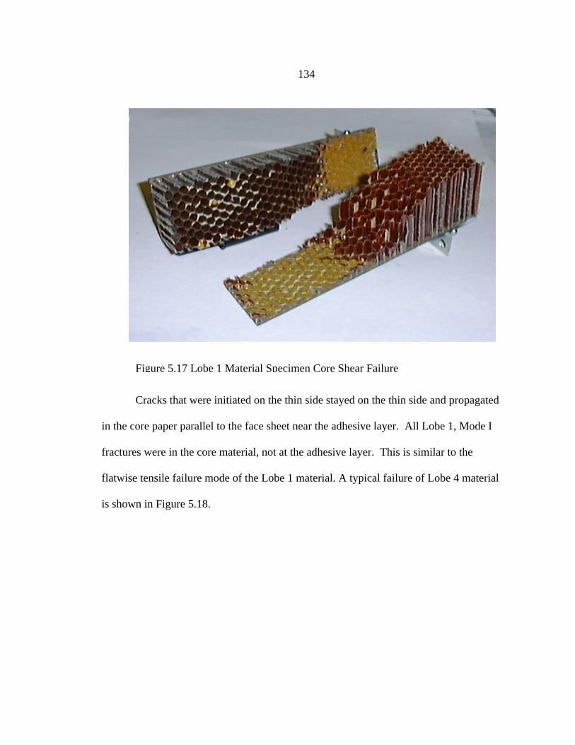
134
Cracks that were initiated on the thin side stayed on the thin side and propagated
in the core paper parallel to the face sheet near the adhesive layer. All Lobe 1, Mode I
fractures were in the core material, not at the adhesive layer. This is similar to the
flatwise tensile failure mode of the Lobe 1 material. A typical failure of Lobe 4 material
is shown in Figure 5.18.
Figure 5.17 Lobe 1 Material Specimen Core Shear Failure
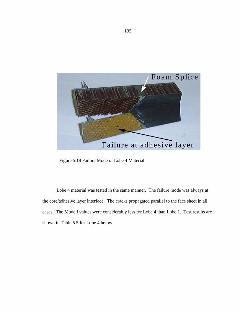
135
Lobe 4 material was tested in the same manner. The failure mode was always at
the core/adhesive layer interface. The cracks propagated parallel to the face sheet in all
cases. The Mode I values were considerably less for Lobe 4 than Lobe 1. Test results are
shown in Table 5.5 for Lobe 4 below.
Foam Sp lice
Failure at adhesive layer
Figure 5.18 Failure Mode of Lobe 4 Material
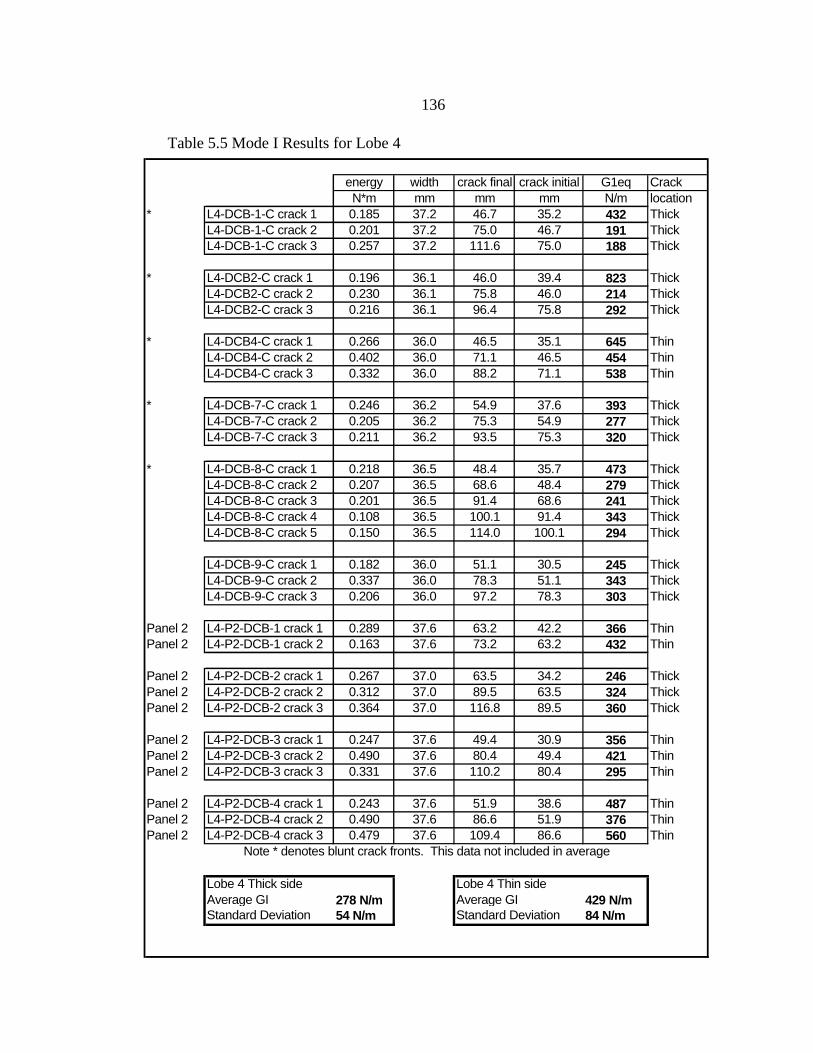
136
Table 5.5 Mode I Results for Lobe 4
energy width crack final crack initial G1eq Crack N*m mm mm mm N/m location
* L4-DCB-1-C crack 1 0.185 37.2 46.7 35.2 432 ThickL4-DCB-1-C crack 2 0.201 37.2 75.0 46.7 191 ThickL4-DCB-1-C crack 3 0.257 37.2 111.6 75.0 188 Thick
* L4-DCB2-C crack 1 0.196 36.1 46.0 39.4 823 ThickL4-DCB2-C crack 2 0.230 36.1 75.8 46.0 214 ThickL4-DCB2-C crack 3 0.216 36.1 96.4 75.8 292 Thick
* L4-DCB4-C crack 1 0.266 36.0 46.5 35.1 645 ThinL4-DCB4-C crack 2 0.402 36.0 71.1 46.5 454 ThinL4-DCB4-C crack 3 0.332 36.0 88.2 71.1 538 Thin
* L4-DCB-7-C crack 1 0.246 36.2 54.9 37.6 393 ThickL4-DCB-7-C crack 2 0.205 36.2 75.3 54.9 277 ThickL4-DCB-7-C crack 3 0.211 36.2 93.5 75.3 320 Thick
* L4-DCB-8-C crack 1 0.218 36.5 48.4 35.7 473 ThickL4-DCB-8-C crack 2 0.207 36.5 68.6 48.4 279 ThickL4-DCB-8-C crack 3 0.201 36.5 91.4 68.6 241 ThickL4-DCB-8-C crack 4 0.108 36.5 100.1 91.4 343 ThickL4-DCB-8-C crack 5 0.150 36.5 114.0 100.1 294 Thick
L4-DCB-9-C crack 1 0.182 36.0 51.1 30.5 245 ThickL4-DCB-9-C crack 2 0.337 36.0 78.3 51.1 343 ThickL4-DCB-9-C crack 3 0.206 36.0 97.2 78.3 303 Thick
Panel 2 L4-P2-DCB-1 crack 1 0.289 37.6 63.2 42.2 366 ThinPanel 2 L4-P2-DCB-1 crack 2 0.163 37.6 73.2 63.2 432 Thin
Panel 2 L4-P2-DCB-2 crack 1 0.267 37.0 63.5 34.2 246 ThickPanel 2 L4-P2-DCB-2 crack 2 0.312 37.0 89.5 63.5 324 ThickPanel 2 L4-P2-DCB-2 crack 3 0.364 37.0 116.8 89.5 360 Thick
Panel 2 L4-P2-DCB-3 crack 1 0.247 37.6 49.4 30.9 356 ThinPanel 2 L4-P2-DCB-3 crack 2 0.490 37.6 80.4 49.4 421 ThinPanel 2 L4-P2-DCB-3 crack 3 0.331 37.6 110.2 80.4 295 Thin
Panel 2 L4-P2-DCB-4 crack 1 0.243 37.6 51.9 38.6 487 ThinPanel 2 L4-P2-DCB-4 crack 2 0.490 37.6 86.6 51.9 376 ThinPanel 2 L4-P2-DCB-4 crack 3 0.479 37.6 109.4 86.6 560 Thin
Lobe 4 Thick side Lobe 4 Thin sideAverage GI 278 N/m Average GI 429 N/mStandard Deviation 54 N/m Standard Deviation 84 N/m
Note * denotes blunt crack fronts. This data not included in average
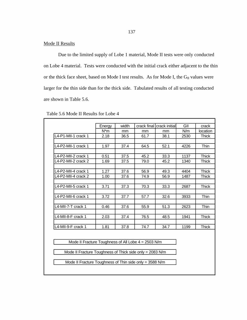
137
Mode II Results
Due to the limited supply of Lobe 1 material, Mode II tests were only conducted
on Lobe 4 material. Tests were conducted with the initial crack either adjacent to the thin
or the thick face sheet, based on Mode I test results. As for Mode I, the GII values were
larger for the thin side than for the thick side. Tabulated results of all testing conducted
are shown in Table 5.6.
Table 5.6 Mode II Results for Lobe 4
Energy width crack final crack initial GII crackN*m mm mm mm N/m location
L4-P1-MII-1 crack 1 2.18 36.5 61.7 38.1 2530 Thick
L4-P2-MII-1 crack 1 1.97 37.4 64.5 52.1 4226 Thin
L4-P2-MII-2 crack 1 0.51 37.5 45.2 33.3 1137 ThickL4-P2-MII-2 crack 2 1.69 37.5 79.0 45.2 1340 Thick
L4-P2-MII-4 crack 1 1.27 37.6 56.9 49.3 4404 ThickL4-P2-MII-4 crack 2 1.00 37.6 74.9 56.9 1487 Thick
L4-P2-MII-5 crack 1 3.71 37.3 70.3 33.3 2687 Thick
L4-P2-MII-6 crack 1 3.72 37.7 57.7 32.6 3933 Thin
L4-MII-7-T crack 1 0.46 37.6 55.9 51.3 2623 Thin
L4-MII-8-F crack 1 2.03 37.4 76.5 48.5 1941 Thick
L4-MII-9-F crack 1 1.81 37.8 74.7 34.7 1199 Thick
Mode II Fracture Toughness of Thick side only = 2083 N/m
Mode II Fracture Toughness of Thin side only = 3588 N/m
Mode II Fracture Toughness of All Lobe 4 = 2503 N/m

138
Discussion of Mode II Results
When only small cracks were grown, a second crack propagation was attempted.
Occasionally, the results from these tests were much larger than for the first. The results
of the repeated crack attempts were less representative than the results from the original
crack session. This case is exactly opposite of Mode I. In Mode I the first crack can be
the least representative, because the initial crack is too blunt or not in path of least
resistance. For the case of Mode II it was very important to ensure that the initial crack
was not blunt, and was following the path of least resistance. As a result, the first attempt
at Mode II delamination had to be perfect. This is because subsequent attempts of crack
propagation typically induced multiple modes of damage other than delamination. When
a material is subjected to multiple modes of failure; the energy absorbed becomes very
large and is not uniquely related to Mode II delamination. This would indicate a much
larger GII value than the material actually possessed.
The average Mode II strain energy release rate for Lobe 4 when the crack was
induced on the thin side was 3590 N/m, and only 2083 N/m for the thick side. The thick
side GII was about 58 % of the thin side GII. This is similar to the Mode I results. The
standard deviation for Mode II was 850 N/m and 1100 N/m for thin and thick
respectively. Despite the large deviation in the results, one point can be made. It is most
likely that the Lobe 4 material would not fail from Mode II fracture. The GII value was
approximately eight times larger that the GI value for each crack configuration. This
indicates that the ability of the material to resist Mode II delamination is approximately
eight times greater than its ability to resist Mode I fracture. If significant bending stresses
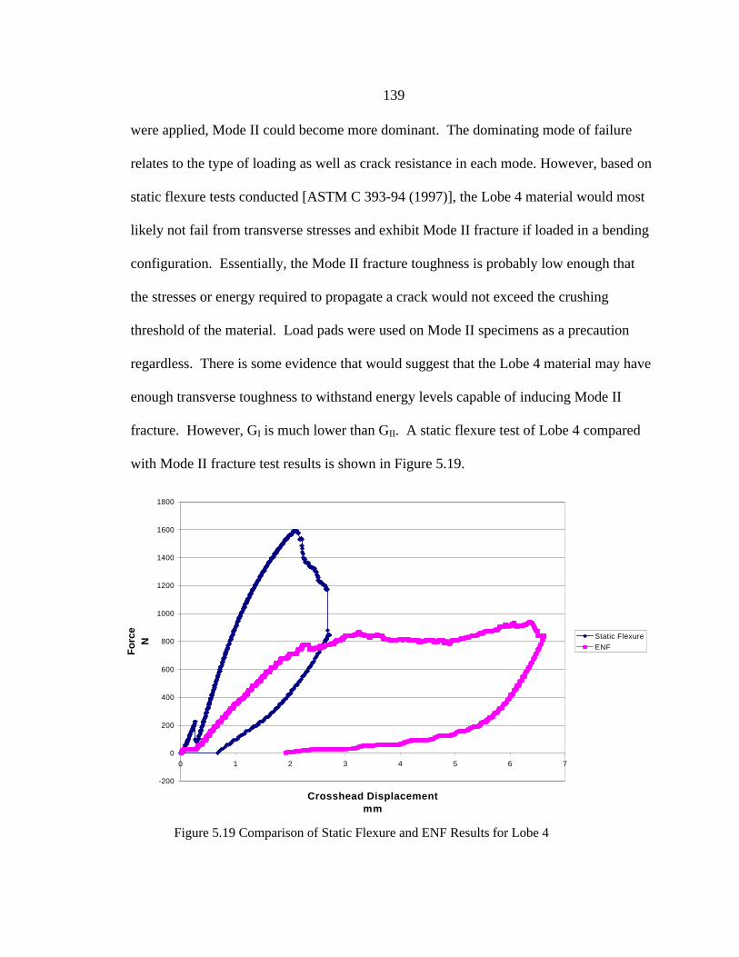
139
were applied, Mode II could become more dominant. The dominating mode of failure
relates to the type of loading as well as crack resistance in each mode. However, based on
static flexure tests conducted [ASTM C 393-94 (1997)], the Lobe 4 material would most
likely not fail from transverse stresses and exhibit Mode II fracture if loaded in a bending
configuration. Essentially, the Mode II fracture toughness is probably low enough that
the stresses or energy required to propagate a crack would not exceed the crushing
threshold of the material. Load pads were used on Mode II specimens as a precaution
regardless. There is some evidence that would suggest that the Lobe 4 material may have
enough transverse toughness to withstand energy levels capable of inducing Mode II
fracture. However, GI is much lower than GII. A static flexure test of Lobe 4 compared
with Mode II fracture test results is shown in Figure 5.19.
-200
0
200
400
600
800
1000
1200
1400
1600
1800
0 1 2 3 4 5 6 7
Crosshead Displacementmm
Fo
rce
N
Static Flexure
ENF
Figure 5.19 Comparison of Static Flexure and ENF Results for Lobe 4
140
Flatwise Compression Results
Flatwise compression tests were also performed as outlined previously. These results
indicated that neither Lobe 1 or Lobe 4 material were equal in compression and tension. The
compressive modulus was lower for compression than for tension. As expected, the compressive
strength for Lobe 4 was larger than its tensile strength. Lobe 1 was opposite with a substantially
lower compressive strength. Lobe 4 had approximately the same compressive strength as Lobe 1
(shown in Table 5.7). If compressive strength were to be required in addition to tensile strength
for combined loading cases, Lobe 4’s significantly lower tensile strength may not be the limiting
property. Three specimens were recycled from Mode I DCBs for Lobe 1 and used for
compression testing. Two Lobe 4 specimens were recycled from panel 1 DCBs and 5 virgin
specimens were also tested. Four virgin Lobe 4 specimens were also taken from panel 2 and
tested. The results for these tests are shown in Table 7. The H/D quantity is the ratio of core
thickness / approximate specimen width.
Discussion of Flatwise Compression Results
The low compression strength of Lobe 1 could be related to the fact that Lobe 1
was thicker than Lobe 4. Having a larger H/D ratio could have caused lower core
buckling loads to occur. Conversely Lobe 4’s performance may be due to its lower H/D
ratio. The compressive failure was most likely simultaneous buckling of cell walls and
was core thickness dependent.
The recycled specimens were probably not affected by the recycling process,
since no damage was present in these regions. Two of Lobe 4’s better data points
regarding modulus and compressive strength are from recycled specimens. These
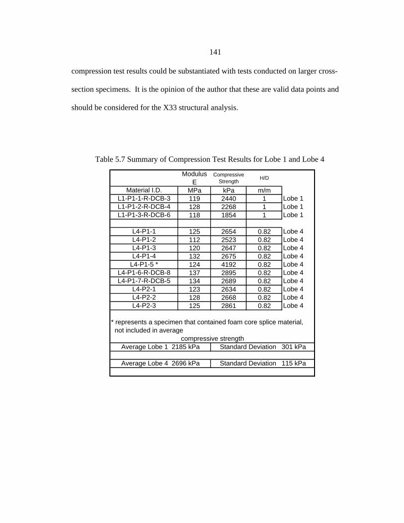
141
compression test results could be substantiated with tests conducted on larger cross-
section specimens. It is the opinion of the author that these are valid data points and
should be considered for the X33 structural analysis.
Table 5.7 Summary of Compression Test Results for Lobe 1 and Lobe 4
Modulus E
Compressive Strength
H/D
Material I.D. MPa kPa m/mL1-P1-1-R-DCB-3 119 2440 1 Lobe 1L1-P1-2-R-DCB-4 128 2268 1 Lobe 1L1-P1-3-R-DCB-6 118 1854 1 Lobe 1
L4-P1-1 125 2654 0.82 Lobe 4L4-P1-2 112 2523 0.82 Lobe 4L4-P1-3 120 2647 0.82 Lobe 4L4-P1-4 132 2675 0.82 Lobe 4
L4-P1-5 * 124 4192 0.82 Lobe 4L4-P1-6-R-DCB-8 137 2895 0.82 Lobe 4L4-P1-7-R-DCB-5 134 2689 0.82 Lobe 4
L4-P2-1 123 2634 0.82 Lobe 4L4-P2-2 128 2668 0.82 Lobe 4L4-P2-3 125 2861 0.82 Lobe 4
* represents a specimen that contained foam core splice material, not included in average
compressive strengthAverage Lobe 1 2185 kPa Standard Deviation 301 kPa
Average Lobe 4 2696 kPa Standard Deviation 115 kPa
142
Numerical Analysis of Honeycomb Fuel Tank Investigation
Motivation
Experimental evaluations of strength and fracture toughness performance were
conducted. Due to the complexity of the honeycomb material some verification of the
experimental findings was needed. In addition to experimental verification, some
validation of the testing techniques was also needed. ASTM standards were followed
closely, however the awkward nature of the sandwich construction required some degree
of originality with regard to testing methodology.
FEA simulations were constructed for the flat-wise tension, mode I, and mode II
testing specimens. Again these simulations were developed to confirm the experimental
data reduction and to insure that the testing methodologies were reasonable. Each of
these models is addressed individually and compared to experimental findings.
Flatwise Tension
Special care was taken when preparing the flatwise tension specimens. The tabs
that were attached were carefully aligned with the aid of a glue fixture to minimize any
bending stress. Eccentric loading would produce a combined stress state and simple
stress equations would provide conservative but errant results. It is virtually impossible
to guarantee exact alignment of loading and very difficult to even measure misalignment.
Instead a FE model of the flatwise tension FWT sample was constructed to evaluate the
effects of misalignment on the tensile stress state.
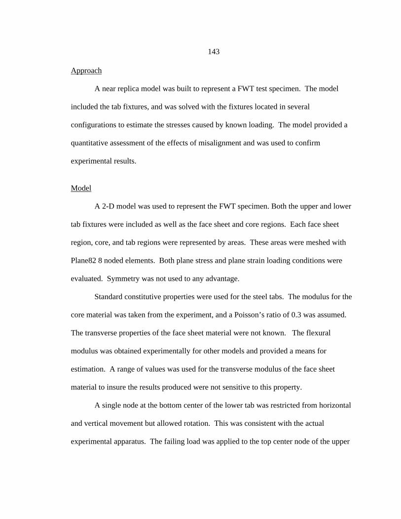
143
Approach
A near replica model was built to represent a FWT test specimen. The model
included the tab fixtures, and was solved with the fixtures located in several
configurations to estimate the stresses caused by known loading. The model provided a
quantitative assessment of the effects of misalignment and was used to confirm
experimental results.
Model
A 2-D model was used to represent the FWT specimen. Both the upper and lower
tab fixtures were included as well as the face sheet and core regions. Each face sheet
region, core, and tab regions were represented by areas. These areas were meshed with
Plane82 8 noded elements. Both plane stress and plane strain loading conditions were
evaluated. Symmetry was not used to any advantage.
Standard constitutive properties were used for the steel tabs. The modulus for the
core material was taken from the experiment, and a Poisson’s ratio of 0.3 was assumed.
The transverse properties of the face sheet material were not known. The flexural
modulus was obtained experimentally for other models and provided a means for
estimation. A range of values was used for the transverse modulus of the face sheet
material to insure the results produced were not sensitive to this property.
A single node at the bottom center of the lower tab was restricted from horizontal
and vertical movement but allowed rotation. This was consistent with the actual
experimental apparatus. The failing load was applied to the top center node of the upper
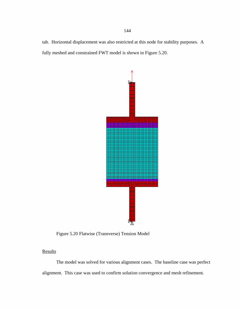
144
tab. Horizontal displacement was also restricted at this node for stability purposes. A
fully meshed and constrained FWT model is shown in Figure 5.20.
Results
The model was solved for various alignment cases. The baseline case was perfect
alignment. This case was used to confirm solution convergence and mesh refinement.
Figure 5.20 Flatwise (Transverse) Tension Model
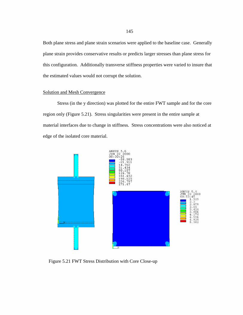
145
Both plane stress and plane strain scenarios were applied to the baseline case. Generally
plane strain provides conservative results or predicts larger stresses than plane stress for
this configuration. Additionally transverse stiffness properties were varied to insure that
the estimated values would not corrupt the solution.
Solution and Mesh Convergence
Stress (in the y direction) was plotted for the entire FWT sample and for the core
region only (Figure 5.21). Stress singularities were present in the entire sample at
material interfaces due to change in stiffness. Stress concentrations were also noticed at
edge of the isolated core material.
Figure 5.21 FWT Stress Distribution with Core Close-up
146
The primary regions of interest were at the facesheet/core interface and in the core itself.
As a result stress profiles were obtained at these regions.
The baseline case was solved for three different mesh sizes. The stress contour
plots of each refinement are shown in Figure 5.34. Similar solutions resulted for each
mesh size, but the most sensitive region was that near the edge. The stress was constant
across the section except for a concentration near the edge. Also at smaller mesh sizes
the curve smoothed and the transition from the isostress state to the concentration was
less abrupt. The plane strain results were similar to the plane stress results, Figure 5.22.
The primary difference was a larger concentration stress at the edge free edge boundary.
0.00
1.00
2.00
3.00
4.00
5.00
6.00
7.00
8.00
0.0 10.0 20.0 30.0 40.0Distance from Left Edge
mm
Str
ess
MP
a
esize = 1
esize = 0.5
esize = 0.25
Figure 5.22 FWT Solution Convergence
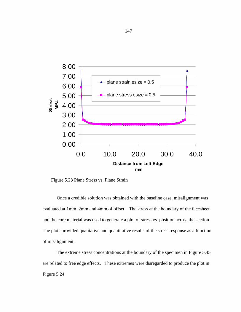
147
Once a credible solution was obtained with the baseline case, misalignment was
evaluated at 1mm, 2mm and 4mm of offset. The stress at the boundary of the facesheet
and the core material was used to generate a plot of stress vs. position across the section.
The plots provided qualitative and quantitative results of the stress response as a function
of misalignment.
The extreme stress concentrations at the boundary of the specimen in Figure 5.45
are related to free edge effects. These extremes were disregarded to produce the plot in
Figure 5.24
0.001.002.003.004.005.006.007.008.00
0.0 10.0 20.0 30.0 40.0Distance from Left Edge
mm
Str
ess
MP
a
plane strain esize = 0.5
plane stress esize = 0.5
Figure 5.23 Plane Stress vs. Plane Strain
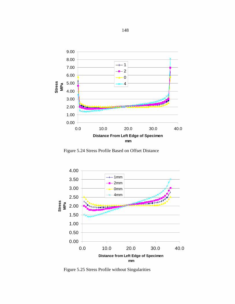
148
0.00
1.00
2.00
3.00
4.00
5.00
6.00
7.00
8.00
9.00
0.0 10.0 20.0 30.0 40.0
Distance From Left Edge of Specimenmm
Str
ess
MP
a 1
2
0
4
Figure 5.24 Stress Profile Based on Offset Distance
0.00
0.50
1.00
1.50
2.00
2.50
3.00
3.50
4.00
0.0 10.0 20.0 30.0 40.0
Distance from Left Edge of Specimenmm
Str
ess
MP
a
1mm
2mm
0mm
4mm
Figure 5.25 Stress Profile without Singularities
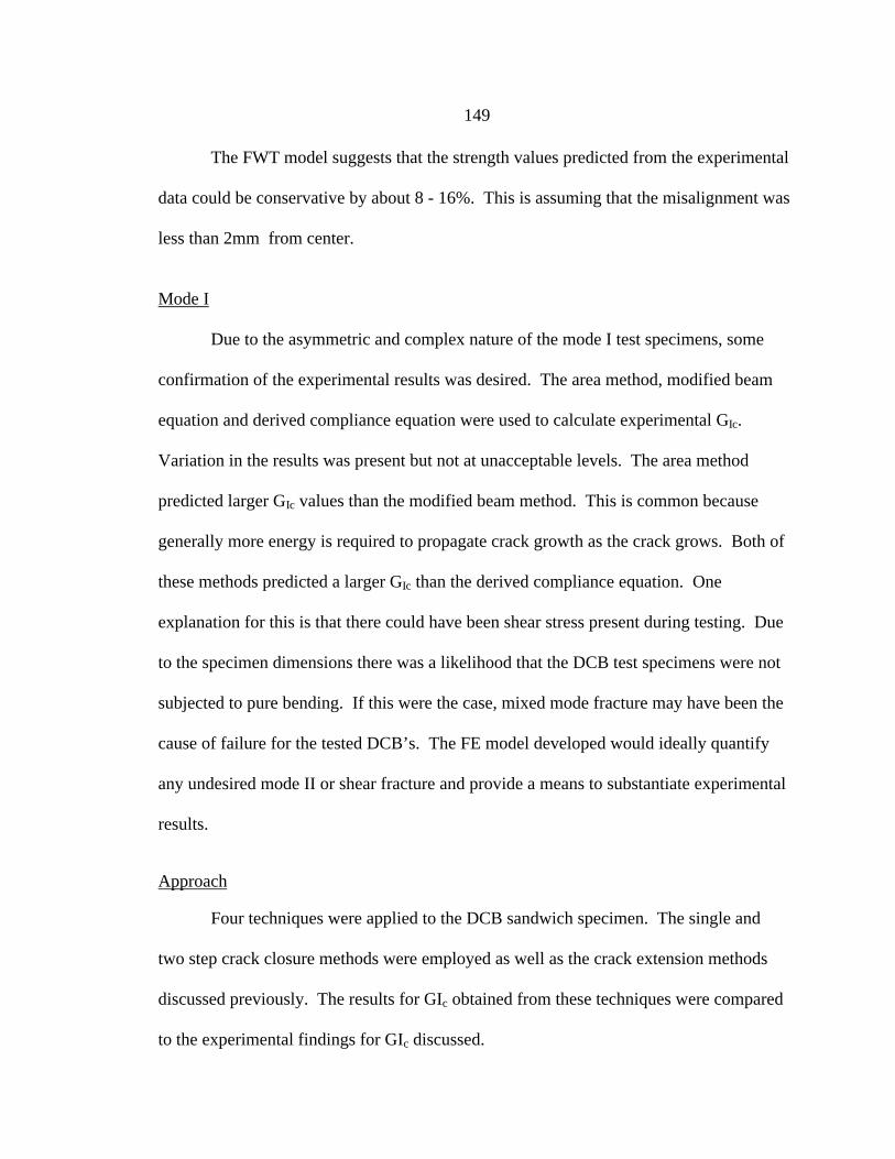
149
The FWT model suggests that the strength values predicted from the experimental
data could be conservative by about 8 - 16%. This is assuming that the misalignment was
less than 2mm from center.
Mode I
Due to the asymmetric and complex nature of the mode I test specimens, some
confirmation of the experimental results was desired. The area method, modified beam
equation and derived compliance equation were used to calculate experimental GIc.
Variation in the results was present but not at unacceptable levels. The area method
predicted larger GIc values than the modified beam method. This is common because
generally more energy is required to propagate crack growth as the crack grows. Both of
these methods predicted a larger GIc than the derived compliance equation. One
explanation for this is that there could have been shear stress present during testing. Due
to the specimen dimensions there was a likelihood that the DCB test specimens were not
subjected to pure bending. If this were the case, mixed mode fracture may have been the
cause of failure for the tested DCB’s. The FE model developed would ideally quantify
any undesired mode II or shear fracture and provide a means to substantiate experimental
results.
Approach
Four techniques were applied to the DCB sandwich specimen. The single and
two step crack closure methods were employed as well as the crack extension methods
discussed previously. The results for GIc obtained from these techniques were compared
to the experimental findings for GIc discussed.

150
Model
Symmetry was immediately abandoned for the DCB analysis. A 2-D model was
developed of the entire honeycomb DCB specimen. A parametric macro procedure was
employed that generated a geometry, which consisted of three regions. Two regions
represented the top and bottom face sheet, and the third region was the core material.
Plane82 (plain strain elements) were used to mesh the areas that comprised these regions.
The DCB was discretized to allow for a refined mesh near the crack zone, and coarser
mesh away from the crack zone. This conserved computational time and maintained
appropriate a/da ratios for fracture analysis.
The face sheet constitutive properties were ascertained empirically by performing
static flexure tests on face sheets removed from previously tested specimens. The core
material properties were estimated and compared to Tri-Core proprietary materials and
did not greatly affect the model.
The nodes corresponding to the hinge attachment locations of the DCB specimen
were restrained from motion in the horizontal direction. The bottom node corresponding
to hinge attachment was additionally constrained from vertical motion, and the critical
force was applied to the top node. No other loads or constraints were required except in
the case of the unit loads for the two step crack closure method. Figure 5.26 contains a
meshed DCB with boundary conditions and loads applied.
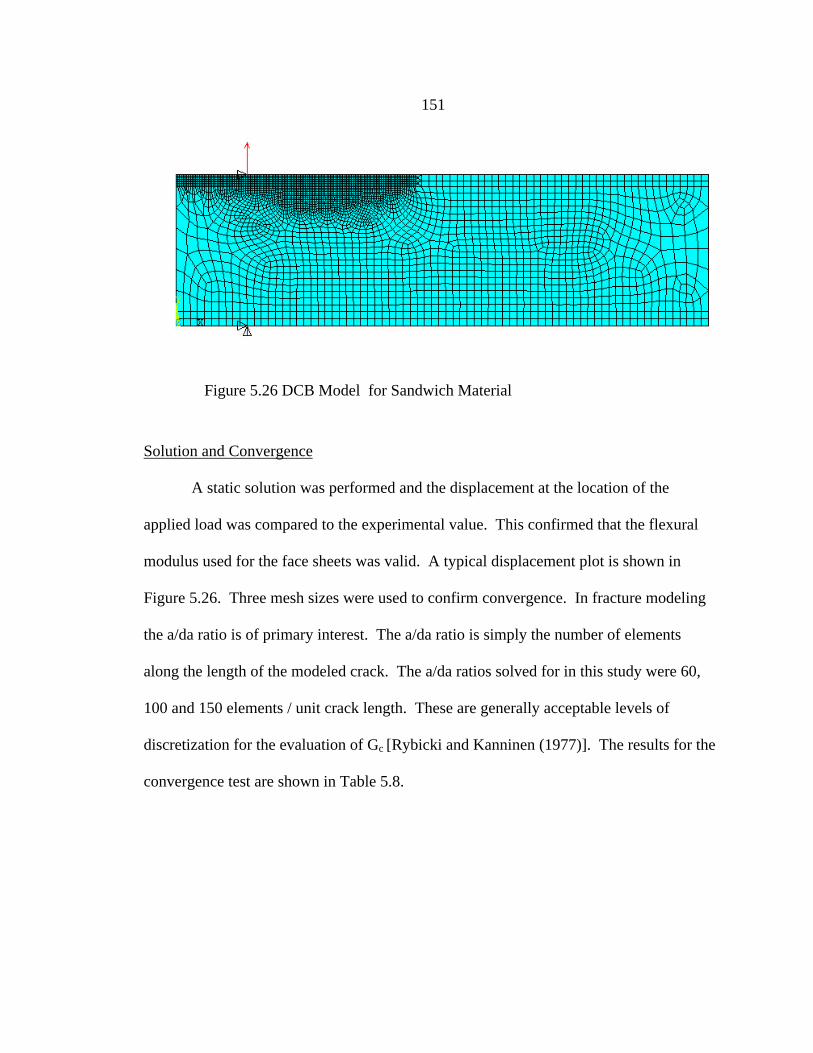
151
Solution and Convergence
A static solution was performed and the displacement at the location of the
applied load was compared to the experimental value. This confirmed that the flexural
modulus used for the face sheets was valid. A typical displacement plot is shown in
Figure 5.26. Three mesh sizes were used to confirm convergence. In fracture modeling
the a/da ratio is of primary interest. The a/da ratio is simply the number of elements
along the length of the modeled crack. The a/da ratios solved for in this study were 60,
100 and 150 elements / unit crack length. These are generally acceptable levels of
discretization for the evaluation of Gc [Rybicki and Kanninen (1977)]. The results for the
convergence test are shown in Table 5.8.
Figure 5.26 DCB Model for Sandwich Material
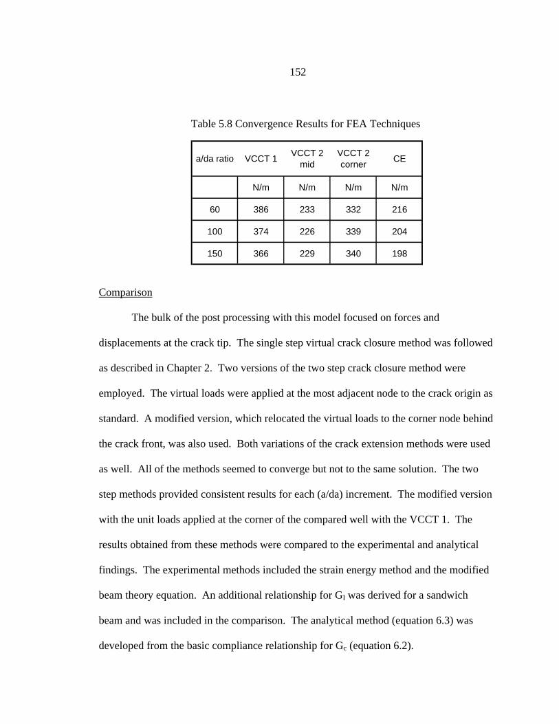
152
Comparison
The bulk of the post processing with this model focused on forces and
displacements at the crack tip. The single step virtual crack closure method was followed
as described in Chapter 2. Two versions of the two step crack closure method were
employed. The virtual loads were applied at the most adjacent node to the crack origin as
standard. A modified version, which relocated the virtual loads to the corner node behind
the crack front, was also used. Both variations of the crack extension methods were used
as well. All of the methods seemed to converge but not to the same solution. The two
step methods provided consistent results for each (a/da) increment. The modified version
with the unit loads applied at the corner of the compared well with the VCCT 1. The
results obtained from these methods were compared to the experimental and analytical
findings. The experimental methods included the strain energy method and the modified
beam theory equation. An additional relationship for GI was derived for a sandwich
beam and was included in the comparison. The analytical method (equation 6.3) was
developed from the basic compliance relationship for Gc (equation 6.2).
Table 5.8 Convergence Results for FEA Techniques
a/da ratio VCCT 1VCCT 2
midVCCT 2 corner
CE
N/m N/m N/m N/m
60 386 233 332 216
100 374 226 339 204
150 366 229 340 198
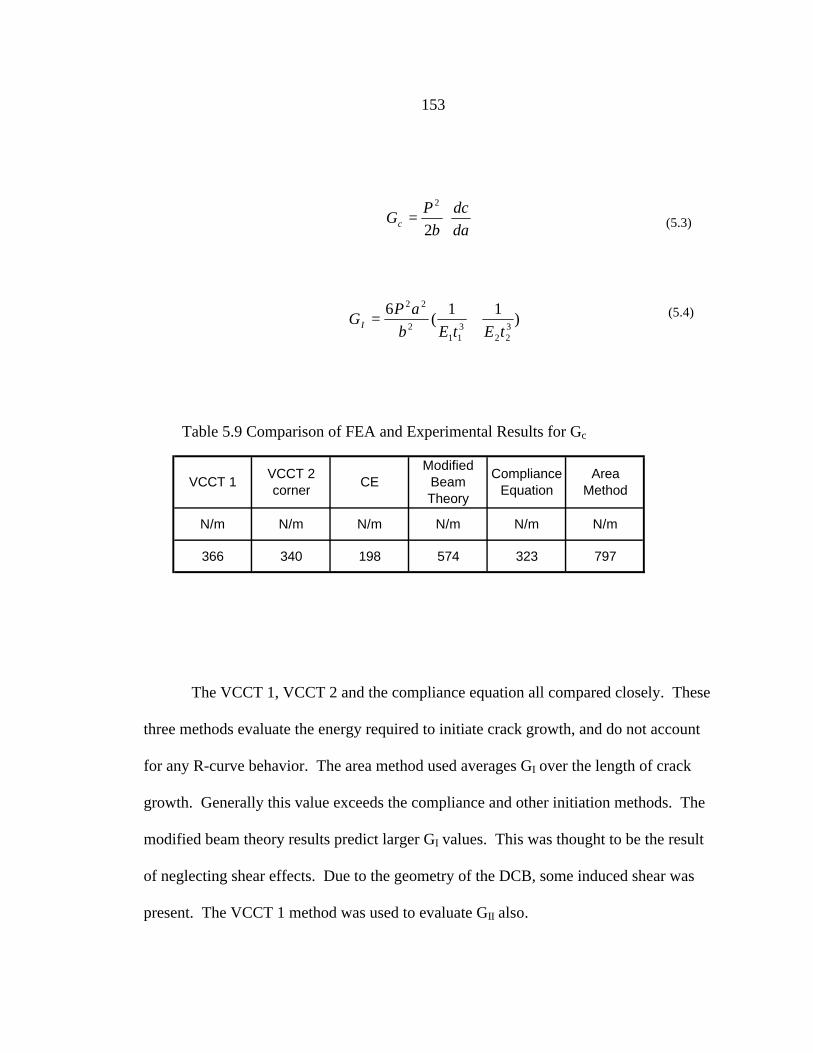
153
The VCCT 1, VCCT 2 and the compliance equation all compared closely. These
three methods evaluate the energy required to initiate crack growth, and do not account
for any R-curve behavior. The area method used averages GI over the length of crack
growth. Generally this value exceeds the compliance and other initiation methods. The
modified beam theory results predict larger GI values. This was thought to be the result
of neglecting shear effects. Due to the geometry of the DCB, some induced shear was
present. The VCCT 1 method was used to evaluate GII also.
VCCT 1VCCT 2 corner
CEModified
Beam Theory
Compliance Equation
Area Method
N/m N/m N/m N/m N/m N/m
366 340 198 574 323 797
Table 5.9 Comparison of FEA and Experimental Results for Gc
da
dc
b
PGc ⋅=
2
2
(5.3)
)11
(6
322
311
2
22
tEtEb
aPGI += (5.4)
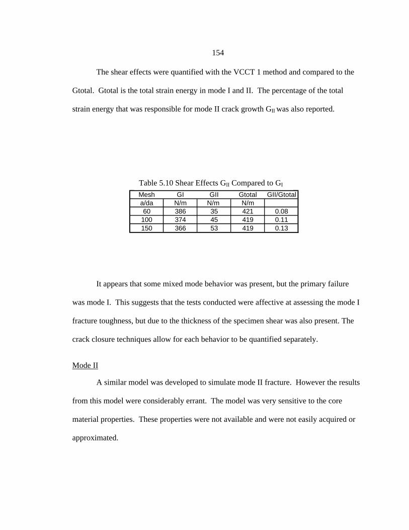
154
The shear effects were quantified with the VCCT 1 method and compared to the
Gtotal. Gtotal is the total strain energy in mode I and II. The percentage of the total
strain energy that was responsible for mode II crack growth GII was also reported.
It appears that some mixed mode behavior was present, but the primary failure
was mode I. This suggests that the tests conducted were affective at assessing the mode I
fracture toughness, but due to the thickness of the specimen shear was also present. The
crack closure techniques allow for each behavior to be quantified separately.
Mode II
A similar model was developed to simulate mode II fracture. However the results
from this model were considerably errant. The model was very sensitive to the core
material properties. These properties were not available and were not easily acquired or
approximated.
Mesh GI GII Gtotal GII/Gtotala/da N/m N/m N/m60 386 35 421 0.08
100 374 45 419 0.11150 366 53 419 0.13
Table 5.10 Shear Effects GII Compared to GI
155
Summary for Case Study II
The variations of the standard testing techniques applied appear to be reasonable.
The screening tests used worked well to characterize the competing material options.
The FWT, FWC, mode I peel test and mode II could be applied to rival material
combinations. Various core materials, face sheet architectures, and adhesive options
could be investigated with these tests and the implementation of the approach provided in
chapter III. The design drivers have been established as well as appropriate tests to
develop a material database of relevant material properties. From this a screening
approach can be applied and potentially some form of analytical prediction may be
pursued with additional development.
The finite element models that were developed validated the experimental
approach for the FWT and mode I testing. The preliminary results from the mode II
model suggest that the experimental GII values are exaggerated. There could have been a
considerable amount of core crushing in addition to crack growth. This would elevate the
experimental GII values. Improvement would have to be made to the existing mode II
FEA model to confirm this suspicion.
The closed form solution developed for evaluating the mode I fracture toughness
of sandwich panels compared well with the FEA solutions. This equation is valid for
asymmetric panels with face sheets of different dimensions and composition. The
equation is valid as long as individual face sheets are not so thin that standard beam
formulations no longer apply.
156
Exploiting sandwich theory to improve specific strength and stiffness works well.
However the laminated nature of this construction and the introduction of an adhesive
layer can make delamination a considerable mode of failure. It would still be difficult at
this point to model and predict discrete crack growth and delamination in primary
structure made of this sandwich type construction. This is especially true for mixed
mode cases [Valisetty (1988)].
Epilogue
It should be noted that, shortly after this investigation was complete, confidence
in honeycomb composite materials had decayed. It was decided to replace the material
investigated in this study with Aluminum [HPC (2001)]. This was pursued only briefly
before the X-33 space shuttle mission was postponed and effectively abandoned or
canceled. This depressing outcome could have most likely been prevented if a thought
process such as those discussed in chapter 3 had been employed.
157
CHAPTER 6
CASE STUDY IIIAEROSPACE RESIN SYSTEM EVALUATION
This project also employed a database – screening approach as in the two
previous case studies. Basic interlaminar properties were evaluated with the procedures
outlined in the background and previous sections. The properties were used to establish a
basic database. The database of fracture properties was used to characterize resin
systems. Special scanning electron microscopy (SEM) technology was used to isolate the
limiting factor of several resin systems.
Project Introduction
ACG is a manufacturer of a complete range of high quality structural prepregs
tailored to meet individual process and application requirements. They are pioneers in
low temperature molding (LTM) epoxy resin systems, providing chemistry for maximum
dimensional accuracy and affordability for both tooling and component applications.
Both low (LTM) and high temperature (HTM) cure resin systems are available that have
a high Tg or glass transition temperature, which allows for use at elevated temperatures.
These systems have unlimited applications but are ideal for aerospace uses.
It is apparent that their lower cure temp high Tg resin systems have significantly
lower fracture toughness than the higher cure temp high Tg systems. Generally, lower
cure temperature resin systems lend themselves to simpler manufacturing processes for
laminate structures, and this makes them desirable.
158
ACG has performed fracture toughness tests to obtain Kc for neat resin coupons.
At this point, the limitation for the performance of the low cure temperature resins is
unknown. A variety of problems could effect the fracture performance of the
manufactured laminates. Chemical incompatibility with the resin systems chosen and the
AS4AP fiber could be a source of limitation. Additionally, the fibers may not be fully
encapsulated by the pre-impregnated resin. Flow characteristics such as viscosity and
other parameters can also effect the fiber resin bond. As stated the resin itself may be the
major limitation and not the resin/fiber interface.
ACG has performed a variety of other tests on prepreg laminates with AS4AP
carbon fiber. At this point most of the mechanical properties are promising. The major
limitation of laminates tested with the AS4AP fiber has been the fracture toughness.
Currently the fracture performance of these combinations has not been optimized and
improvements are welcomed. ACG hopes to improve the fracture toughness of their
AS4AP systems without sacrificing high temperature capabilities. In addition to meeting
these requirements the system should also maintain other mechanical properties such as
flexural stiffness and tensile strength.
Problem Statement
The goal of Montana State University was to quantify the interlaminar
performance of several resin systems. Standard mode I, static mode II, and dynamic
mode II tests were conducted to evaluate the interlaminar fracture toughness. These
procedures were applied to 9 different specimen types at several post-cure conditions.
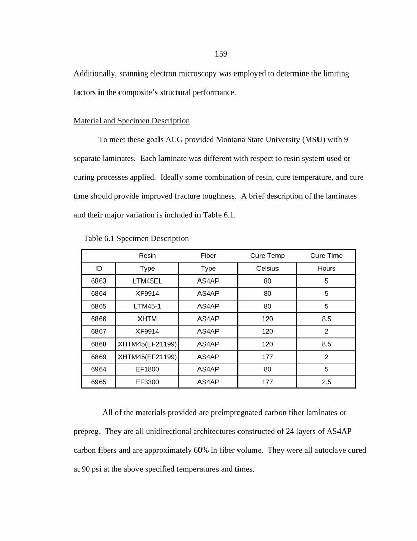
159
Additionally, scanning electron microscopy was employed to determine the limiting
factors in the composite’s structural performance.
Material and Specimen Description
To meet these goals ACG provided Montana State University (MSU) with 9
separate laminates. Each laminate was different with respect to resin system used or
curing processes applied. Ideally some combination of resin, cure temperature, and cure
time should provide improved fracture toughness. A brief description of the laminates
and their major variation is included in Table 6.1.
All of the materials provided are preimpregnated carbon fiber laminates or
prepreg. They are all unidirectional architectures constructed of 24 layers of AS4AP
carbon fibers and are approximately 60% in fiber volume. They were all autoclave cured
at 90 psi at the above specified temperatures and times.
Resin Fiber Cure Temp Cure Time
ID Type Type Celsius Hours
6863 LTM45EL AS4AP 80 5
6864 XF9914 AS4AP 80 5
6865 LTM45-1 AS4AP 80 5
6866 XHTM AS4AP 120 8.5
6867 XF9914 AS4AP 120 2
6868 XHTM45(EF21199) AS4AP 120 8.5
6869 XHTM45(EF21199) AS4AP 177 2
6964 EF1800 AS4AP 80 5
6965 EF3300 AS4AP 177 2.5
Table 6.1 Specimen Description
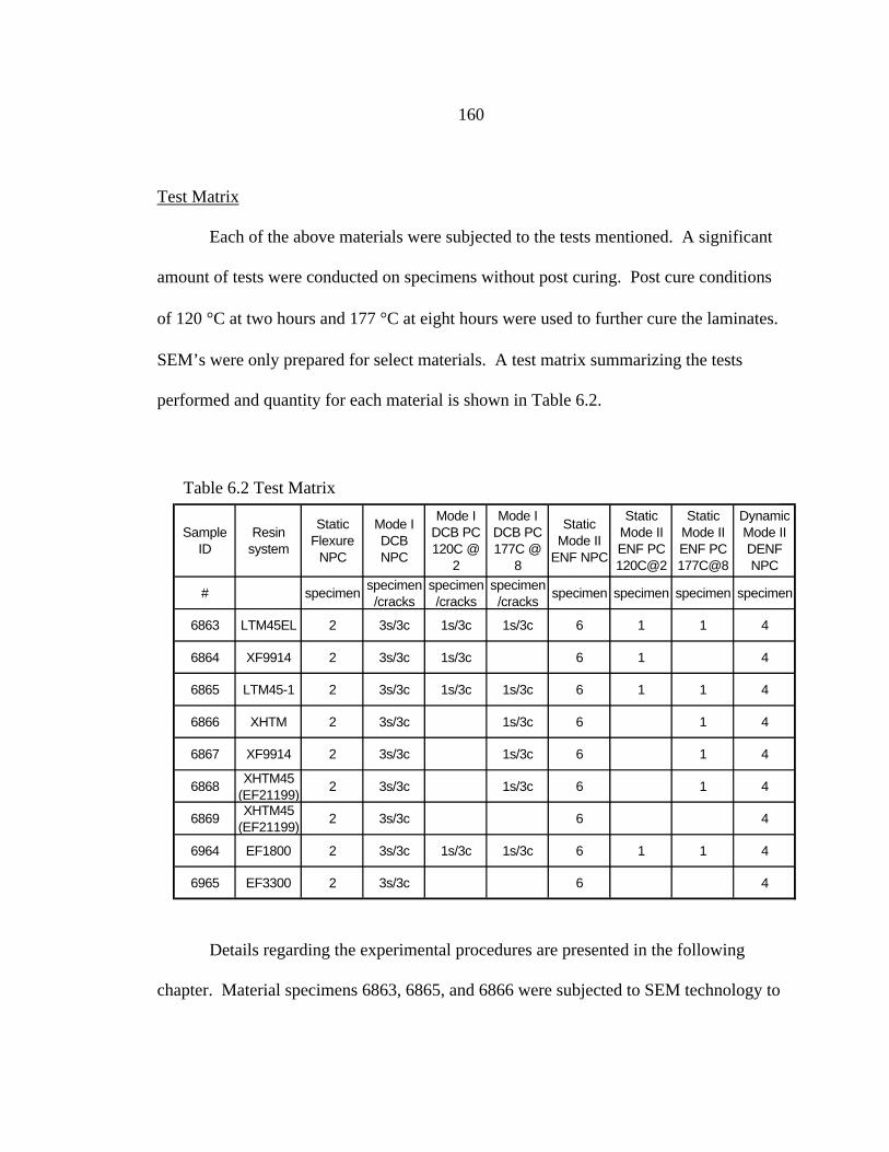
160
Test Matrix
Each of the above materials were subjected to the tests mentioned. A significant
amount of tests were conducted on specimens without post curing. Post cure conditions
of 120 °C at two hours and 177 °C at eight hours were used to further cure the laminates.
SEM’s were only prepared for select materials. A test matrix summarizing the tests
performed and quantity for each material is shown in Table 6.2.
Details regarding the experimental procedures are presented in the following
chapter. Material specimens 6863, 6865, and 6866 were subjected to SEM technology to
Sample ID
Resin system
Static Flexure
NPC
Mode I DCB NPC
Mode I DCB PC 120C @
2
Mode I DCB PC 177C @
8
Static Mode II
ENF NPC
Static Mode II ENF PC 120C@2
Static Mode II ENF PC 177C@8
Dynamic Mode II DENF NPC
# specimenspecimen/cracks
specimen/cracks
specimen/cracks
specimen specimen specimen specimen
6863 LTM45EL 2 3s/3c 1s/3c 1s/3c 6 1 1 4
6864 XF9914 2 3s/3c 1s/3c 6 1 4
6865 LTM45-1 2 3s/3c 1s/3c 1s/3c 6 1 1 4
6866 XHTM 2 3s/3c 1s/3c 6 1 4
6867 XF9914 2 3s/3c 1s/3c 6 1 4
6868XHTM45
(EF21199)2 3s/3c 1s/3c 6 1 4
6869XHTM45
(EF21199)2 3s/3c 6 4
6964 EF1800 2 3s/3c 1s/3c 1s/3c 6 1 1 4
6965 EF3300 2 3s/3c 6 4
Table 6.2 Test Matrix
161
investigate bond interface issues. This was done at non-postcured state and at the
extreme postcure condition of 177 °C for 8 hours.
Experimental Methods
Static flexure experiments were performed in addition to several fracture
toughness evaluations. The procedure, data reduction methods, and explanation of the
procedures are provided in this chapter.
Static Flexure
Static flexure (SF) experiments were initially performed. The primary material
properties obtained from this test, are the flexural modulus and the flexural strength. The
major goal of ACG is to improve fracture toughness without compromising strength and
stiffness. Additionally, some of the data reduction methods for fracture toughness require
the value for the elastic modulus. In the case of composites, the flexural modulus is used
for this. Performing static flexure tests also provided a means to establish confidence in
testing apparatus and a baseline to compare to ACG’s results.
Static Flexure Apparatus
An in-house produced 3-point fixture was used in combination with the model
4206 Instron screw type test device. The device was screw driven and can be used in
load or displacement control. The static test apparatus is shown in Figure 4.10. The
voltage proportional to load applied and displacement were output and sampled by a
SCXI-1200 labview data acquisition system.
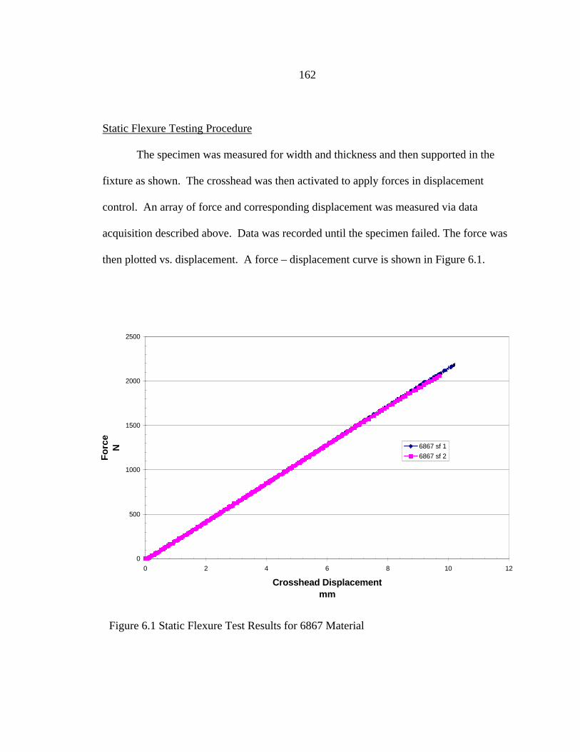
162
Static Flexure Testing Procedure
The specimen was measured for width and thickness and then supported in the
fixture as shown. The crosshead was then activated to apply forces in displacement
control. An array of force and corresponding displacement was measured via data
acquisition described above. Data was recorded until the specimen failed. The force was
then plotted vs. displacement. A force – displacement curve is shown in Figure 6.1.
0
500
1000
1500
2000
2500
0 2 4 6 8 10 12
Crosshead Displacementmm
Fo
rce
N 6867 sf 1
6867 sf 2
Figure 6.1 Static Flexure Test Results for 6867 Material
163
Static Flexure Data Reduction
From the graphical output in Figure 6.1 the bending modulus and maximum
bending stress were determined using standard beam theory formulations [Gere (1984)]
provided in equations (4.4 and 4.7). The bending modulus was obtained by performing a
curve fit on the linear portion of the flexure data. This slope was equivalent to the spring
stiffness. The maximum load was used to calculate the flexure strength or bending
strength of each material.
Fracture Toughness Testing
The fracture toughness tests conducted consisted of static mode I, static mode II,
and dynamic mode II. Strain energy release rates were evaluated from each experiment.
Strain rate dependencies were investigated, as well as postcure temperature affects. The
procedures are discussed briefly here and in more detail in the background (Chapter 2).
DCB Testing Procedure
All of the prepreg laminates supplied had MR1 release film placed at the outer
edge. This release film was inserted at the midplane to represent a flaw or crack.
Specimens were then sectioned from a composite plate and their dimensions were
150mm x 25mm with a thickness of about 3.2 mm. Once the specimens were acquired
from the plate, hinges were attached at the cracked end with Hysol.EA 9309.2NA QT
adhesive. A fixture was used to connect the hinge equipped DCB specimen to standard
Instron Grips. The specimen was then pulled slowly apart in displacement control at a
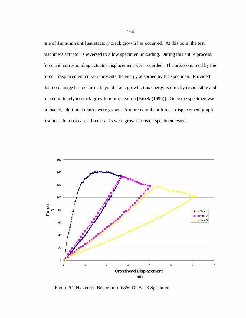
164
rate of 1mm/min until satisfactory crack growth has occurred. At this point the test
machine’s actuator is reversed to allow specimen unloading. During this entire process,
force and corresponding actuator displacement were recorded. The area contained by the
force – displacement curve represents the energy absorbed by the specimen. Provided
that no damage has occurred beyond crack growth, this energy is directly responsible and
related uniquely to crack growth or propagation [Broek (1996)]. Once the specimen was
unloaded, additional cracks were grown. A more compliant force – displacement graph
resulted. In most cases three cracks were grown for each specimen tested.
0
20
40
60
80
100
120
140
160
0 1 2 3 4 5 6 7
Crosshead Displacementmm
Fo
rce
N
crack 1
crack 2
crack 3
Figure 6.2 Hysteretic Behavior of 6866 DCB – 3 Specimen
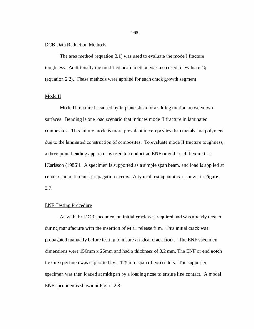
165
DCB Data Reduction Methods
The area method (equation 2.1) was used to evaluate the mode I fracture
toughness. Additionally the modified beam method was also used to evaluate GI
(equation 2.2). These methods were applied for each crack growth segment.
Mode II
Mode II fracture is caused by in plane shear or a sliding motion between two
surfaces. Bending is one load scenario that induces mode II fracture in laminated
composites. This failure mode is more prevalent in composites than metals and polymers
due to the laminated construction of composites. To evaluate mode II fracture toughness,
a three point bending apparatus is used to conduct an ENF or end notch flexure test
[Carlsson (1986)]. A specimen is supported as a simple span beam, and load is applied at
center span until crack propagation occurs. A typical test apparatus is shown in Figure
2.7.
ENF Testing Procedure
As with the DCB specimen, an initial crack was required and was already created
during manufacture with the insertion of MR1 release film. This initial crack was
propagated manually before testing to insure an ideal crack front. The ENF specimen
dimensions were 150mm x 25mm and had a thickness of 3.2 mm. The ENF or end notch
flexure specimen was supported by a 125 mm span of two rollers. The supported
specimen was then loaded at midspan by a loading nose to ensure line contact. A model
ENF specimen is shown in Figure 2.8.
166
The load was incremented in displacement control until the crack propagated.
Mode II crack propagation is typically confirmed by the presence of audible cracking and
is generally not stable. The crack propagated to the midspan, or further, immediately and
repeat crack growths were not possible. The hysteretic behavior of unloading was
captured, an example is shown in Figure 6.3.
ENF Data Reduction Methods
As in the case of mode I type fracture, the driving element of crack growth is
strain energy. The energy method, equation (2.2), is valid for mode II fracture as well.
0
100
200
300
400
500
600
700
800
0.00 0.50 1.00 1.50 2.00 2.50 3.00 3.50 4.00
Crosshead or Actuator Displacementmm
Lo
ad N
Figure 6.3 Mode II Crack Behavior with Hysteresis Captured
167
The load displacement data can be integrated and divided by the crack damage area to
calculate a GII or mode II fracture toughness as before.
Dynamic Mode II Testing
Dynamic resistance to delamination was evaluated using dynamic mode II testing.
The metric of this experiment is still GIIc, but for dynamic loading conditions. This
property accounts for any strain rate dependencies of the material [Cairns (1992)].
Dynamic ENF Apparatus
To conduct a dynamic version of the mode II fracture toughness test, special
equipment had to be used [Mackin (1992) and McMichael (1988)]. An impact tower was
employed to supply the force and energy to induce crack growth (Figure 4.1). Special
data acquisition equipment was also used (Figure 4.2). Details regarding the equipment
used follow.
Dynamic ENF Testing Procedure
Most of the procedure and data reduction techniques are similar to the mode II
fracture toughness methods outlined in Chapter 2 and for ENF testing. The test specimen
geometry is the same as the ENF. An ultrasonic transducer was used to isolate and
measure crack fronts before and after testing. The primary difference of the DENF test
from the ENF test is method of applying force. As discussed, load is applied by means of
an impactor travelling at speeds of about 1 m/s. The impact force is sampled at high
frequencies (50 kHz). A typical impact trace is shown in Figure 6.4.
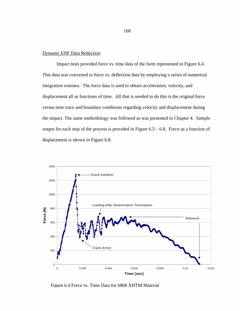
168
Dynamic ENF Data Reduction
Impact tests provided force vs. time data of the form represented in Figure 6.4.
This data was converted to force vs. deflection data by employing a series of numerical
integration routines. The force data is used to obtain acceleration, velocity, and
displacement all as functions of time. All that is needed to do this is the original force
versus time trace and boundary conditions regarding velocity and displacement during
the impact. The same methodology was followed as was presented in Chapter 4. Sample
output for each step of the process is provided in Figure 6.5 – 6.8. Force as a function of
displacement is shown in Figure 6.8.
0
200
400
600
800
1000
1200
1400
0 0.002 0.004 0.006 0.008 0.01 0.012
Time (sec)
Fo
rce
(N)
Crack Initiation
Crack Arrest
Rebound
Loading After Delamination Termination
Figure 6.4 Force vs. Time Data for 6868 XHTM Material
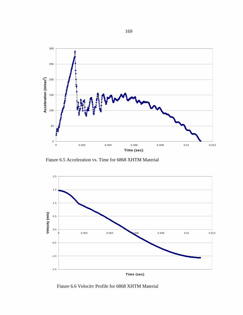
169
0
50
100
150
200
250
300
0 0.002 0.004 0.006 0.008 0.01 0.012
Time (sec)
Acc
eler
atio
n (
m/s
ec2 )
Figure 6.5 Acceleration vs. Time for 6868 XHTM Material
-1.5
-1.0
-0.5
0.0
0.5
1.0
1.5
2.0
0 0.002 0.004 0.006 0.008 0.01 0.012
Time (sec)
Vel
oci
ty (
m/s
)
Figure 6.6 Velocity Profile for 6868 XHTM Material
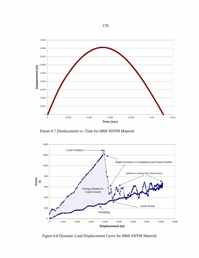
170
0
0.001
0.002
0.003
0.004
0.005
0.006
0.007
0.008
0.009
0 0.002 0.004 0.006 0.008 0.01 0.012
Time (sec)
Dis
pla
cem
ent
(m)
Figure 6.7 Displacement vs. Time for 6868 XHTM Material
0
200
400
600
800
1000
1200
1400
0 0.001 0.002 0.003 0.004 0.005 0.006 0.007 0.008 0.009
Displacement (m)
Fo
rce
N
Crack Initiation
Rapid Increase in Compliance and Crack Growth
Crack Arrest
Unloading
Additional Loading After Delamination
Energy Related to Crack Growth
Figure 6.8 Dynamic Load Displacement Curve for 6868 XHTM Material
171
The data reduction techniques outlined in chapter 2 were followed. Both the area
method (equation 2.2) and the compliance method (equation 2.6) were used to obtain
experimental GII values.
Scanning Electron Microscopy Evaluations
Scanning Electron Microscopy (SEM) technology was used to isolate the
limitation of the interlaminar performance of several select materials provided [Hyer
(1998)]. Bondability (or compatibility of the resin and fiber) and brittle resin behavior
were the most likely culprits.
SEM Apparatus
Special equipment at the Montana State University (MSU) Image and Chemistry
Analysis Laboratory (ICAL) facility were employed to capture images of fracture planes
of GII specimens. Special Assistant Nancy Equall and a state of the art scanning electron
microscope were the primary components of this system.
SEM Testing Procedure
Samples of three different materials were subjected to SEM evaluations for two
extreme postcure conditions (not postcured and postcured at 177 °C for 8 hours). These
samples were sectioned from GII specimen remnants. Their dimensions were
approximately 12mm x 25mm. Upon sectioning these samples they were sprayed with
compressed nitrogen gas to remove debree from sectioning. Once the specimens were
cleaned and mounted on aluminum platforms, they were subjected to a “sputtering”
process. This process consisted of using argon gas to induce ionic excitement and
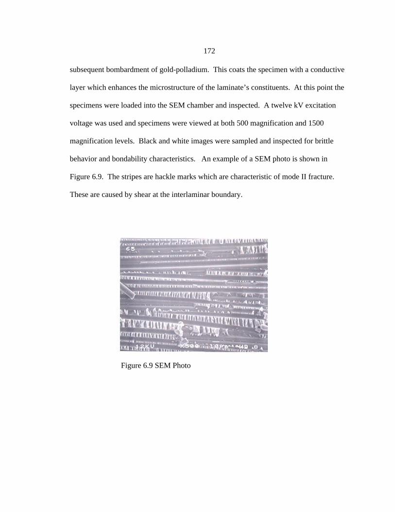
172
subsequent bombardment of gold-polladium. This coats the specimen with a conductive
layer which enhances the microstructure of the laminate’s constituents. At this point the
specimens were loaded into the SEM chamber and inspected. A twelve kV excitation
voltage was used and specimens were viewed at both 500 magnification and 1500
magnification levels. Black and white images were sampled and inspected for brittle
behavior and bondability characteristics. An example of a SEM photo is shown in
Figure 6.9. The stripes are hackle marks which are characteristic of mode II fracture.
These are caused by shear at the interlaminar boundary.
Figure 6.9 SEM Photo
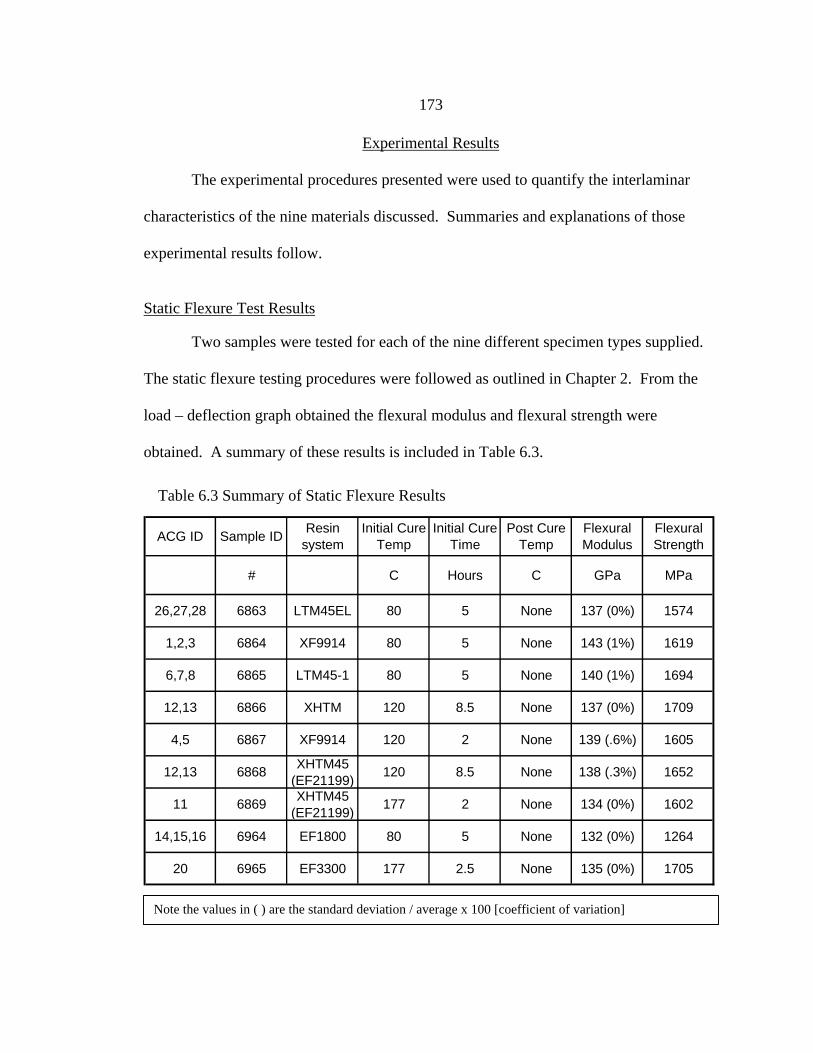
173
Experimental Results
The experimental procedures presented were used to quantify the interlaminar
characteristics of the nine materials discussed. Summaries and explanations of those
experimental results follow.
Static Flexure Test Results
Two samples were tested for each of the nine different specimen types supplied.
The static flexure testing procedures were followed as outlined in Chapter 2. From the
load – deflection graph obtained the flexural modulus and flexural strength were
obtained. A summary of these results is included in Table 6.3.
Table 6.3 Summary of Static Flexure Results
ACG ID Sample IDResin
systemInitial Cure
TempInitial Cure
TimePost Cure
TempFlexural Modulus
Flexural Strength
# C Hours C GPa MPa
26,27,28 6863 LTM45EL 80 5 None 137 (0%) 1574
1,2,3 6864 XF9914 80 5 None 143 (1%) 1619
6,7,8 6865 LTM45-1 80 5 None 140 (1%) 1694
12,13 6866 XHTM 120 8.5 None 137 (0%) 1709
4,5 6867 XF9914 120 2 None 139 (.6%) 1605
12,13 6868XHTM45
(EF21199)120 8.5 None 138 (.3%) 1652
11 6869XHTM45
(EF21199)177 2 None 134 (0%) 1602
14,15,16 6964 EF1800 80 5 None 132 (0%) 1264
20 6965 EF3300 177 2.5 None 135 (0%) 1705
Note the values in ( ) are the standard deviation / average x 100 [coefficient of variation]
174
The modulus values were very consistent and precise for all of the specimen
tested. The flexural modulus values ranged from 132-143 GPa. The flexural strength
values followed similarly with greater variation amongst each specimen type and
comparatively between all of the specimen. The 6964 series possessed the worst flexural
strength of 1290 MPa and the 6866 (XHTM) was the best at 1709 MPa.
Mode I Results from DCB Testing
Three specimen of each type were subjected to standard Double Cantilever Beam
(DCB) testing to evaluate (GI). The testing procedure in Chapter 2 was followed. The
crack was initially grown and usually extended two more times. Each specimen provided
three samples or data for GI. The Mode I fracture toughness (GII) was calculated by both
methods presented in Chapter 2. The compliance method represents the energy required
to initiate crack growth. The area method averages the energy required to extend a crack
some distance. Generally, the area method provides a larger value for GI. This is
because of R-curve behavior or a material’s inherent ability to arrest crack growth as
discussed previously. Fiber bridging and other mechanisms contribute to this. Materials
that do not exhibit this behavior will generally have unstable and continuous crack
growth in service. The results for the Mode I tests conducted are shown in Table 6.4.
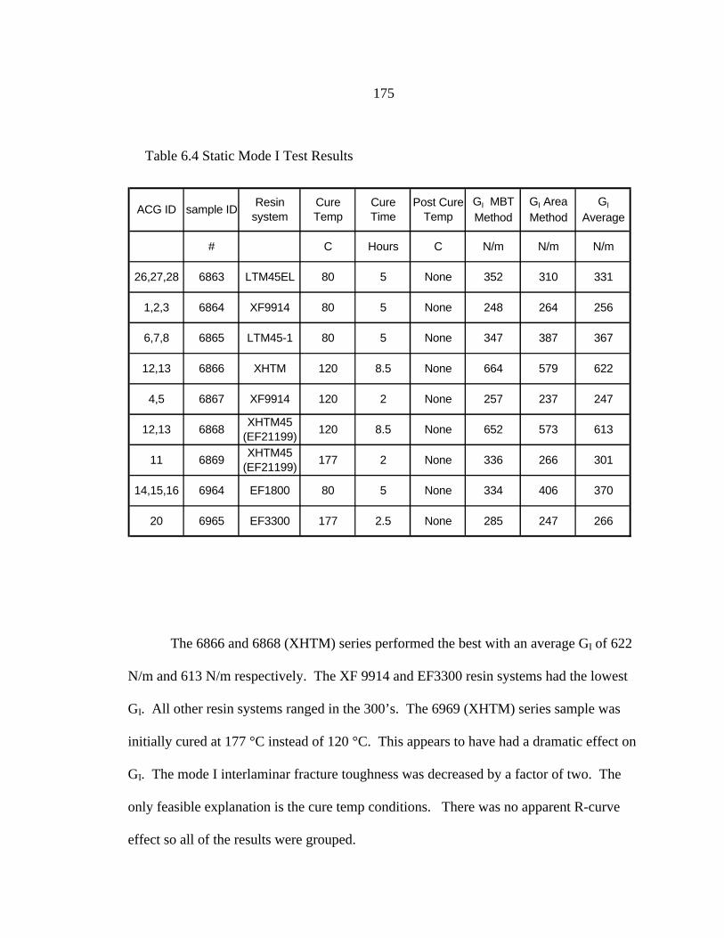
175
The 6866 and 6868 (XHTM) series performed the best with an average GI of 622
N/m and 613 N/m respectively. The XF 9914 and EF3300 resin systems had the lowest
GI. All other resin systems ranged in the 300’s. The 6969 (XHTM) series sample was
initially cured at 177 °C instead of 120 °C. This appears to have had a dramatic effect on
GI. The mode I interlaminar fracture toughness was decreased by a factor of two. The
only feasible explanation is the cure temp conditions. There was no apparent R-curve
effect so all of the results were grouped.
Table 6.4 Static Mode I Test Results
ACG ID sample IDResin
systemCure Temp
Cure Time
Post Cure Temp
GI MBT Method
GI Area Method
GI
Average
# C Hours C N/m N/m N/m
26,27,28 6863 LTM45EL 80 5 None 352 310 331
1,2,3 6864 XF9914 80 5 None 248 264 256
6,7,8 6865 LTM45-1 80 5 None 347 387 367
12,13 6866 XHTM 120 8.5 None 664 579 622
4,5 6867 XF9914 120 2 None 257 237 247
12,13 6868XHTM45
(EF21199)120 8.5 None 652 573 613
11 6869XHTM45
(EF21199)177 2 None 336 266 301
14,15,16 6964 EF1800 80 5 None 334 406 370
20 6965 EF3300 177 2.5 None 285 247 266
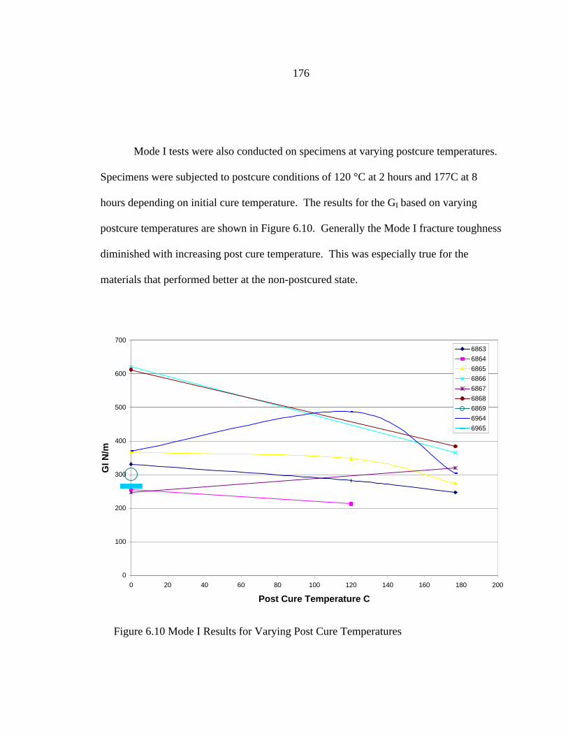
176
Mode I tests were also conducted on specimens at varying postcure temperatures.
Specimens were subjected to postcure conditions of 120 °C at 2 hours and 177C at 8
hours depending on initial cure temperature. The results for the GI based on varying
postcure temperatures are shown in Figure 6.10. Generally the Mode I fracture toughness
diminished with increasing post cure temperature. This was especially true for the
materials that performed better at the non-postcured state.
0
100
200
300
400
500
600
700
0 20 40 60 80 100 120 140 160 180 200
Post Cure Temperature C
GI N
/m
6863
6864
6865
6866
6867
6868
6869
6964
6965
Figure 6.10 Mode I Results for Varying Post Cure Temperatures
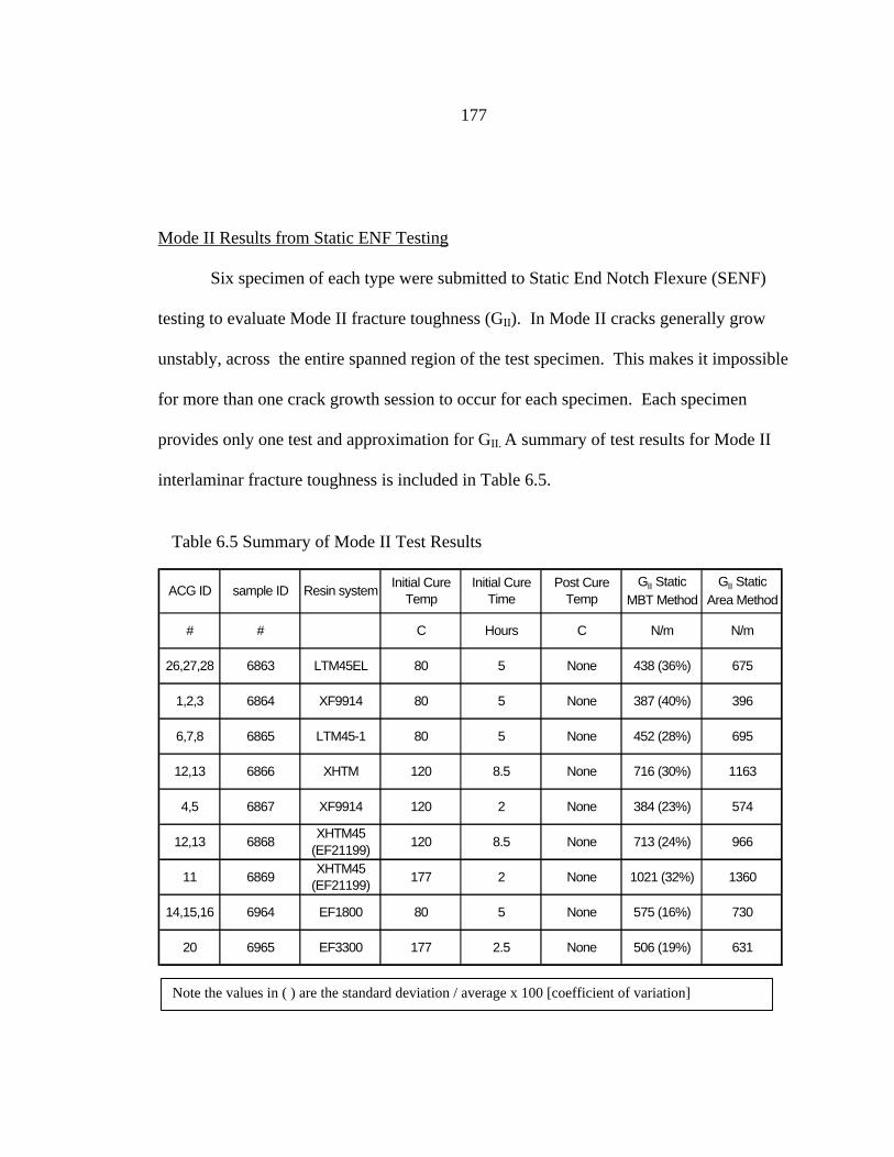
177
Mode II Results from Static ENF Testing
Six specimen of each type were submitted to Static End Notch Flexure (SENF)
testing to evaluate Mode II fracture toughness (GII). In Mode II cracks generally grow
unstably, across the entire spanned region of the test specimen. This makes it impossible
for more than one crack growth session to occur for each specimen. Each specimen
provides only one test and approximation for GII. A summary of test results for Mode II
interlaminar fracture toughness is included in Table 6.5.
Note the values in ( ) are the standard deviation / average x 100 [coefficient of variation]
ACG ID sample ID Resin systemInitial Cure
TempInitial Cure
TimePost Cure
Temp GII Static
MBT MethodGII Static
Area Method
# # C Hours C N/m N/m
26,27,28 6863 LTM45EL 80 5 None 438 (36%) 675
1,2,3 6864 XF9914 80 5 None 387 (40%) 396
6,7,8 6865 LTM45-1 80 5 None 452 (28%) 695
12,13 6866 XHTM 120 8.5 None 716 (30%) 1163
4,5 6867 XF9914 120 2 None 384 (23%) 574
12,13 6868XHTM45
(EF21199)120 8.5 None 713 (24%) 966
11 6869XHTM45
(EF21199)177 2 None 1021 (32%) 1360
14,15,16 6964 EF1800 80 5 None 575 (16%) 730
20 6965 EF3300 177 2.5 None 506 (19%) 631
Table 6.5 Summary of Mode II Test Results
178
The mode II results indicate that the (XHTM) series, 6866, 6868, and 6869
materials performed the best. For mode II the 6869 material (with the higher initial cure
temperature) performed better than the 6866 or 6868. This suggests that increasing the
initial cure temperature could improve GII but be detrimental to GI. In all cases, the area
method provided a larger GII value than the compliance equation. This indicates that all
the materials possess some inherent crack arresting attributes.
SENF tests were also performed on several of the materials at varying post cure
temperatures. Post curing the composites at higher temperatures might have reduced the
interlaminar fracture toughness as for mode I. However, SENF tests were conducted at
the same conditions as for mode I, and opposite results were obtained. The results of this
are shown in Figure 6.11.
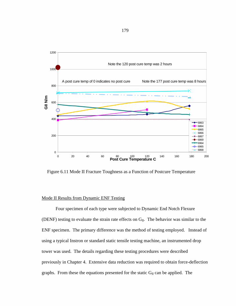
179
Mode II Results from Dynamic ENF Testing
Four specimen of each type were subjected to Dynamic End Notch Flexure
(DENF) testing to evaluate the strain rate effects on GII. The behavior was similar to the
ENF specimen. The primary difference was the method of testing employed. Instead of
using a typical Instron or standard static tensile testing machine, an instrumented drop
tower was used. The details regarding these testing procedures were described
previously in Chapter 4. Extensive data reduction was required to obtain force-deflection
graphs. From these the equations presented for the static GII can be applied. The
Figure 6.11 Mode II Fracture Toughness as a Function of Postcure Temperature
0
200
400
600
800
1000
1200
0 20 40 60 80 100 120 140 160 180 200Post Cure Temperature C
GII
N/m
686368646865686668676869696469656868
Note the 120 post cure temp was 2 hours
Note the 177 post cure temp was 8 hoursA post cure temp of 0 indicates no post cure
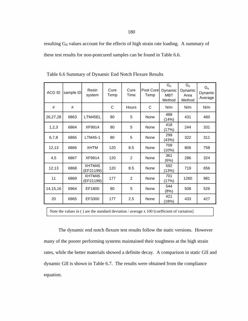
180
resulting GII values account for the effects of high strain rate loading. A summary of
these test results for non-postcured samples can be found in Table 6.6.
The dynamic end notch flexure test results follow the static versions. However
many of the poorer performing systems maintained their toughness at the high strain
rates, while the better materials showed a definite decay. A comparison in static GII and
dynamic GII is shown in Table 6.7. The results were obtained from the compliance
equation.
Table 6.6 Summary of Dynamic End Notch Flexure Results
ACG ID sample IDResin
systemCure Temp
Cure Time
Post Cure Temp
GII
Dynamic MBT
Method
GII
Dynamic Area
Method
GII
Dynamic Average
# # C Hours C N/m N/m N/m
26,27,28 6863 LTM45EL 80 5 None489
(14%)431 460
1,2,3 6864 XF9914 80 5 None418
(17%)244 331
6,7,8 6865 LTM45-1 80 5 None299
(43%)322 311
12,13 6866 XHTM 120 8.5 None709
(10%)806 758
4,5 6867 XF9914 120 2 None361 (6%)
286 324
12,13 6868XHTM45
(EF21199)120 8.5 None
592 (13%)
719 656
11 6869XHTM45
(EF21199)177 2 None
701 (17%)
1260 981
14,15,16 6964 EF1800 80 5 None544 (8%)
508 526
20 6965 EF3300 177 2.5 None421
(18%)433 427
Note the values in ( ) are the standard deviation / average x 100 [coefficient of variation]

181
A definite rate dependency was noticed, but not for all of the materials. The
LTM-45 (6865) and the XHTM-45 (6868 and 6869) series showed reduced performance
in mode II at high strain rates. The other materials were mostly unaffected by the
increased strain rate. The dynamic end notch flexure test results have a lower coefficient
of variation due to the use of ultrasonic crack detection throughout the course of the
experiments.
Table 6.7 Rate Dependency Comparison for Mode II Testing
Note the values in ( ) are the standard deviation / average x 100 [coefficient of variation]
ACG IDSample
IDResin
system
Initial Cure Temp
Initial Cure Time
Post Cure Temp
GII Static MBT
Method
GII
Dynamic MBT
Method
GII
static / dynamic
# # C Hours C N/m N/m none
26,27,28 6863 LTM45EL 80 5 None 438 (36%) 489 (14%) 0.90
1,2,3 6864 XF9914 80 5 None 387 (40%) 418 (17%) 0.93
6,7,8 6865 LTM45-1 80 5 None 452 (28%) 299 (43%) 1.51
12,13 6866 XHTM 120 8.5 None 716 (30%) 709 (10%) 1.01
4,5 6867 XF9914 120 2 None 384 (23%) 361 (6%) 1.06
12,13 6868XHTM45 (EF21199
120 8.5 None 713 (24%) 592 (13%) 1.20
11 6869XHTM45 (EF21199
177 2 None 1021 (32%)701 (17%) 1.46
14,15,16 6964 EF1800 80 5 None 575 (16%) 544 (8%) 1.06
20 6965 EF3300 177 2.5 None 506 (19%) 421 (18%) 1.20

182
SEM Results for Selected Systems
Three specimen types were prepared for Scanning Electron Microscope (SEM)
analysis. The 6863, 6865, and 6866 materials were prepared based on the procedures
presented. The goal of this particular investigation was to determine if the interlaminar
performance was linked to or limited by the interface or bond properties of the resin to
the fibers.
Photographs were taken at both a 500 magnification and a 1500 magnification.
Images were captured for the above specimen types from samples sectioned from mode II
remnants. This was done for specimens, which had been post-cured at 177C, and for
those that had not been post-cured at all. It was demonstrated that post curing had an
effect on the interlaminar fracture toughness. Possibly there might be a relationship
between the micro-mechanics of the composites, post cure temperature, and their
interlaminar performance.
The results of the SEM photos are very subjective. The goal of the interpretation
of these results is to find some evidence of brittle resin behavior and also to investigate
the apparent bondability or compatibility of the fibers and resin systems. Each of the
three resin systems investigated will be discussed individually.
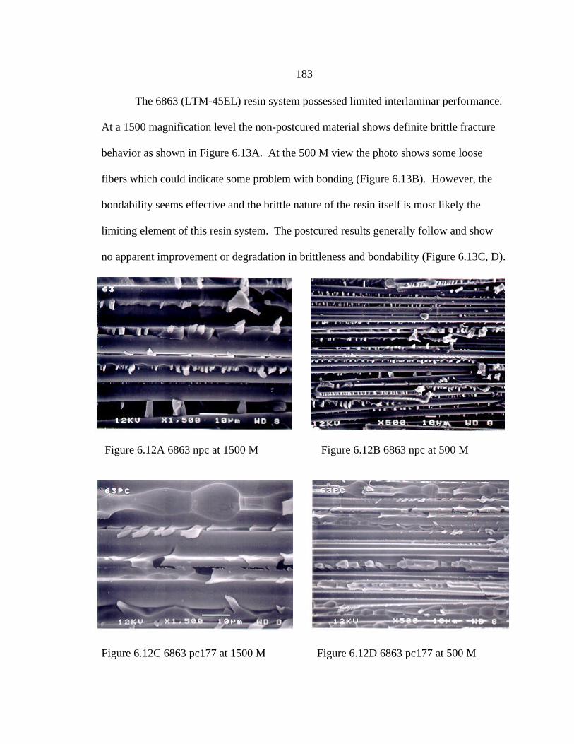
183
The 6863 (LTM-45EL) resin system possessed limited interlaminar performance.
At a 1500 magnification level the non-postcured material shows definite brittle fracture
behavior as shown in Figure 6.13A. At the 500 M view the photo shows some loose
fibers which could indicate some problem with bonding (Figure 6.13B). However, the
bondability seems effective and the brittle nature of the resin itself is most likely the
limiting element of this resin system. The postcured results generally follow and show
no apparent improvement or degradation in brittleness and bondability (Figure 6.13C, D).
Figure 6.12A 6863 npc at 1500 M Figure 6.12B 6863 npc at 500 M
Figure 6.12C 6863 pc177 at 1500 M Figure 6.12D 6863 pc177 at 500 M
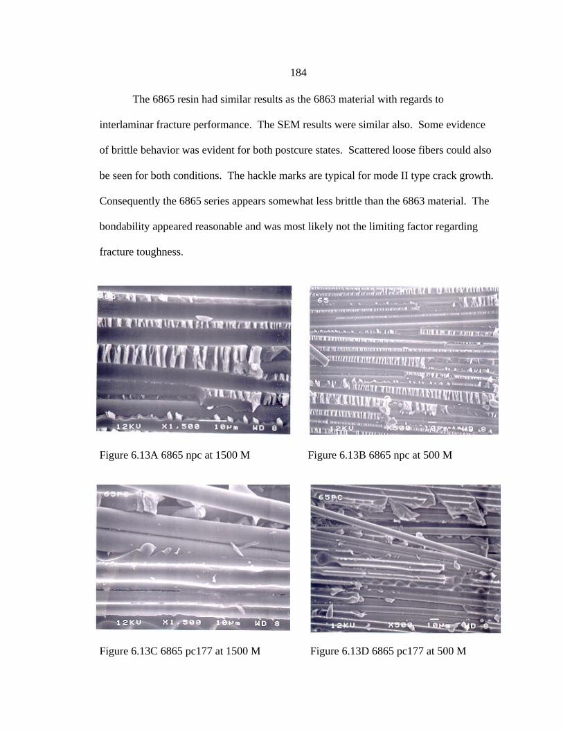
184
The 6865 resin had similar results as the 6863 material with regards to
interlaminar fracture performance. The SEM results were similar also. Some evidence
of brittle behavior was evident for both postcure states. Scattered loose fibers could also
be seen for both conditions. The hackle marks are typical for mode II type crack growth.
Consequently the 6865 series appears somewhat less brittle than the 6863 material. The
bondability appeared reasonable and was most likely not the limiting factor regarding
fracture toughness.
Figure 6.13A 6865 npc at 1500 M Figure 6.13B 6865 npc at 500 M
Figure 6.13C 6865 pc177 at 1500 M Figure 6.13D 6865 pc177 at 500 M
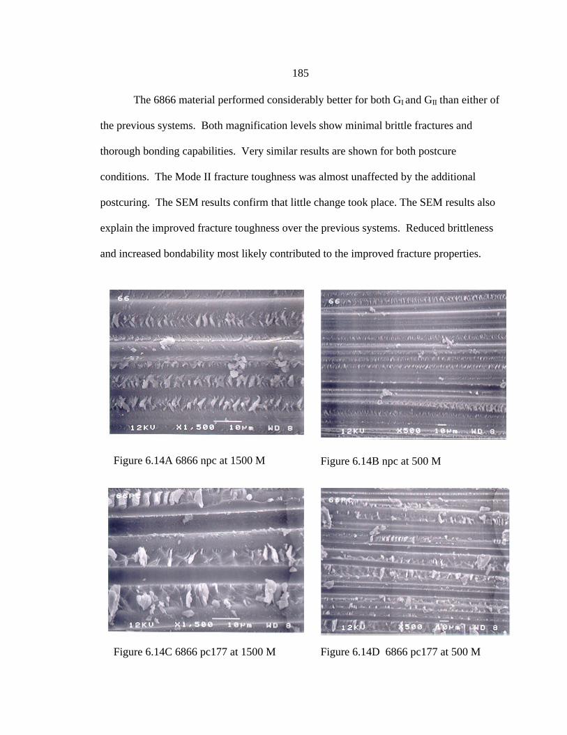
185
The 6866 material performed considerably better for both GI and GII than either of
the previous systems. Both magnification levels show minimal brittle fractures and
thorough bonding capabilities. Very similar results are shown for both postcure
conditions. The Mode II fracture toughness was almost unaffected by the additional
postcuring. The SEM results confirm that little change took place. The SEM results also
explain the improved fracture toughness over the previous systems. Reduced brittleness
and increased bondability most likely contributed to the improved fracture properties.
Figure 6.14A 6866 npc at 1500 M Figure 6.14B npc at 500 M
Figure 6.14C 6866 pc177 at 1500 M Figure 6.14D 6866 pc177 at 500 M
186
Summary for Case Study III
Nine separate laminates, of different resin compositions, were provided to MSU
by ACG for interlaminar fracture toughness evaluations. Mode I, mode II and dynamic
mode II delamination experiments were performed. The results of these experiments
indicate that the XHTM resin system or high temperature molded laminates outperformed
the LTM systems with regard to overall fracture toughness.
However, when the specimens were subjected to postcuring, most of the materials
GI or mode I fracture toughness decayed. The XHTM systems lost a greater percentage
of toughness than the LTM systems. This was not true for mode II, GII values typically
held steady or improved with the addition postcuring. Possibly the resins shear strength
is less effected than the tensile strength.
Reduced performance at higher strain rates was not noticed for most materials.
The dynamic GII values followed the static results closely except for the 6865 or LTM45-
1 system and the XHTM45 systems.
The SEM tests provided some correlation between interlaminar fracture
performance and microstructure. The 6863, 6865 and 6866 systems were compared. The
6863 (LTM45EL) system and the 6865 (LTM45-1) system were similar in composition
and fracture performance. Both showed signs of brittle resin fracture, and some problems
with bondability. The 6866 (XHTM45) system outperformed both the 6863 and 6865
system and showed improved bondability and less brittle fracture.
This case study was the perfect application for the database-screening process
presented in Figures 3.4 and 3.5. The materials investigated possessed good mechanical
properties and all had similar strength and stiffness metrics.
187
However, significant variation was found with regard to interlaminar fracture
performance. The Mode I values did not always follow the Mode II values either. This
reinforces the need to conduct both tests. It was also discovered that some of the
materials exhibited a definite rate sensitivity. As a result, when composite candidates are
to be used in impact or dynamic environments, the dynamic Mode II tests should also be
used to characterize the laminate. The resin post cure effects indicate that interlaminar
fracture performance can also be altered by processing details. The SEM technology
worked well to relate the interlaminar behavior to the micro-mechanics of the laminate.
This technique of damage assessment can be used with the database-screening process to
optimize a potential laminate composite. Ultimately, the methodology outlined could be
employed to further improve and optimize the laminated architectures that are currently
being produced as well as future candidate engineering materials.
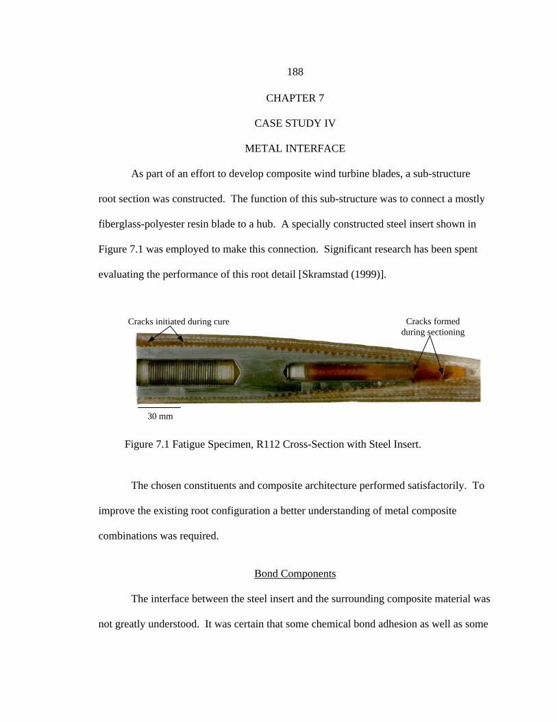
188
CHAPTER 7
CASE STUDY IV
METAL INTERFACE
As part of an effort to develop composite wind turbine blades, a sub-structure
root section was constructed. The function of this sub-structure was to connect a mostly
fiberglass-polyester resin blade to a hub. A specially constructed steel insert shown in
Figure 7.1 was employed to make this connection. Significant research has been spent
evaluating the performance of this root detail [Skramstad (1999)].
The chosen constituents and composite architecture performed satisfactorily. To
improve the existing root configuration a better understanding of metal composite
combinations was required.
Bond Components
The interface between the steel insert and the surrounding composite material was
not greatly understood. It was certain that some chemical bond adhesion as well as some
30 mm
Cracks formedduring sectioning
Cracks initiated during cure
Figure 7.1 Fatigue Specimen, R112 Cross-Section with Steel Insert.
189
structural interlock joined the steel insert to the composite material. The importance and
contribution of each was unknown.
Chemical Bond
Since the steel insert was typically placed in the fabric and the resin was then
injected via RTM, the steel was primarily held in place by the resin system used. The
resin then possessed a molecular or chemical bond to the steel. This bond would allow
load in form of shear to transfer from the blade to the root and ultimately the hub. It is
surmised that chemical bonding is not solely responsible for this load transfer from the
insert material to the surrounding composite. Due to the geometry of the insert a definite
structural mechanism also exists that secures the insert to the composite housing.
Structural Interlock
The threaded surface of the insert material provides mechanical interlock. This
mechanical interlock enhances the bond strength of the insert material beyond chemical
adhesion alone. In fact during initial stages of root development, it was observed that the
steel insert would fail before the composite material or the bond itself.
Need for Simpler Structure and Methodology
In order to improve upon existing design or to even understand its success, more
information is needed regarding both chemical bond properties and mechanical interface
properties. As a screening process, two new test specimens were developed and
constructed. These scaled down structures were designed to reduce the burden of
constructing an entire root section to evaluate potential modifications. The simplest test
190
specimen is the shear lap specimen. This test isolates chemical bond strength. A more
complex test specimen was developed to account for the mechanical interface between
metals and composites. This specimen was called the miniroot. This is a scaled down
version of the root section specimen mentioned.
Lap Shear
Two types of lap shear tests were investigated. A single lap shear and a double
lap shear test were used. These tests are generally used for adhesives. However, resin
systems share some of the same type of structural responsibility as adhesives. Details
regarding each are discussed individually.
Single Lap Shear
The single lap shear test specimen has been designed to evaluate bond properties
of adhesives. ASTM standards are in place that provide guidelines and procedures for
conducting this test [ASTM D1002-72 (1993)]. The shear lap test is used to evaluate and
quantify an adhesive strength of a joining material with a given material. Typically, a lap
or overlap joint is made by two pieces of parent material and a bond is formed with the
adhesive. These are specimen that can then be pulled apart in shear. Shear is the basic
mechanism of load transfer for adhesives and glues. A shear strength can then be
obtained from the failing load and the bond area.
Generally, this is not a material property and designing with these values can be
hazardous [ASTM D4896-89 (1993)]. Other tests exists that provide more meaningful
results, but are difficult to conduct and require complicated fixtures [ASTM D3983-92
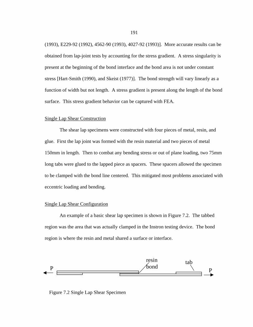
191
(1993), E229-92 (1992), 4562-90 (1993), 4027-92 (1993)]. More accurate results can be
obtained from lap-joint tests by accounting for the stress gradient. A stress singularity is
present at the beginning of the bond interface and the bond area is not under constant
stress [Hart-Smith (1990), and Skeist (1977)]. The bond strength will vary linearly as a
function of width but not length. A stress gradient is present along the length of the bond
surface. This stress gradient behavior can be captured with FEA.
Single Lap Shear Construction
The shear lap specimens were constructed with four pieces of metal, resin, and
glue. First the lap joint was formed with the resin material and two pieces of metal
150mm in length. Then to combat any bending stress or out of plane loading, two 75mm
long tabs were glued to the lapped piece as spacers. These spacers allowed the specimen
to be clamped with the bond line centered. This mitigated most problems associated with
eccentric loading and bending.
Single Lap Shear Configuration
An example of a basic shear lap specimen is shown in Figure 7.2. The tabbed
region was the area that was actually clamped in the Instron testing device. The bond
region is where the resin and metal shared a surface or interface.
tabresinbond
PP
Figure 7.2 Single Lap Shear Specimen
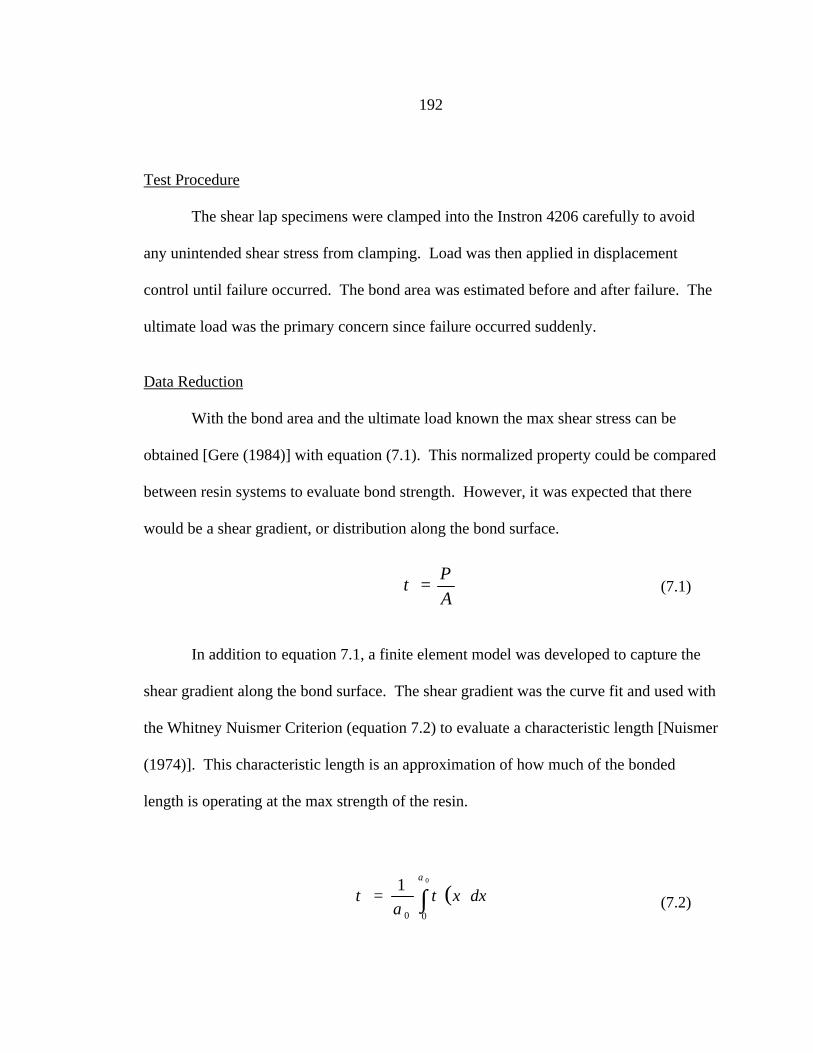
192
Test Procedure
The shear lap specimens were clamped into the Instron 4206 carefully to avoid
any unintended shear stress from clamping. Load was then applied in displacement
control until failure occurred. The bond area was estimated before and after failure. The
ultimate load was the primary concern since failure occurred suddenly.
Data Reduction
With the bond area and the ultimate load known the max shear stress can be
obtained [Gere (1984)] with equation (7.1). This normalized property could be compared
between resin systems to evaluate bond strength. However, it was expected that there
would be a shear gradient, or distribution along the bond surface.
In addition to equation 7.1, a finite element model was developed to capture the
shear gradient along the bond surface. The shear gradient was the curve fit and used with
the Whitney Nuismer Criterion (equation 7.2) to evaluate a characteristic length [Nuismer
(1974)]. This characteristic length is an approximation of how much of the bonded
length is operating at the max strength of the resin.
(7.1)A
P=τ
( )∫=0
00
1a
dxxa
ττ (7.2)
193
Double Lap Shear
The single lap shear test coupon provides limited results [ASTM D4896-89
(1993), Hart-Smith (1990), Skeist (1977)]. Many agree that the test results from the SLS
specimens are good for screening analysis or baseline comparison only. The primary
limitation of this test is the peel stresses induced from eccentric loading of the
asymmetric geometry. Other variables that affect the results are; the thickness of the
adhesive and adherend, the stiffness of the adherend, and the bond length.
A new lap specimen has been developed to combat these issues [Hart-Smith
(1990)] called the inverse skin doubler specimen. The primary limitation of this
specimen is its complexity and machining requirements. Features include tapered inside
and outside faces of metal adherends to reduce peel stresses at the edge. The specimen is
also symmetric which reduces bending stresses.
This study employed a modified shear lap specimen, which has been called a
double lap shear specimen (DLS). The double lap shear specimen is a symmetric version
of the single lap specimen. It shares some of the same features as the inverse skin
doubler specimen, but does not have tapered adherends. The DLS specimen was used to
confirm the SLS test results and should provide more accurate results due to the
mitigation of bending.
Double Lap Shear Configuration
The DLS specimens were almost as simple as the SLS specimen. The primary
difference was that a second bond interface had to be introduced to maintain symmetry.
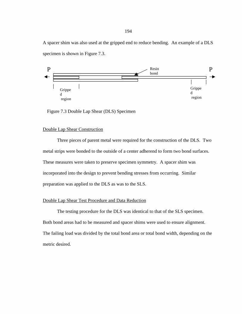
194
A spacer shim was also used at the gripped end to reduce bending. An example of a DLS
specimen is shown in Figure 7.3.
Double Lap Shear Construction
Three pieces of parent metal were required for the construction of the DLS. Two
metal strips were bonded to the outside of a center adherend to form two bond surfaces.
These measures were taken to preserve specimen symmetry. A spacer shim was
incorporated into the design to prevent bending stresses from occurring. Similar
preparation was applied to the DLS as was to the SLS.
Double Lap Shear Test Procedure and Data Reduction
The testing procedure for the DLS was identical to that of the SLS specimen.
Both bond areas had to be measured and spacer shims were used to ensure alignment.
The failing load was divided by the total bond area or total bond width, depending on the
metric desired.
PP Resinbond
Gripped region
Gripped region
Figure 7.3 Double Lap Shear (DLS) Specimen
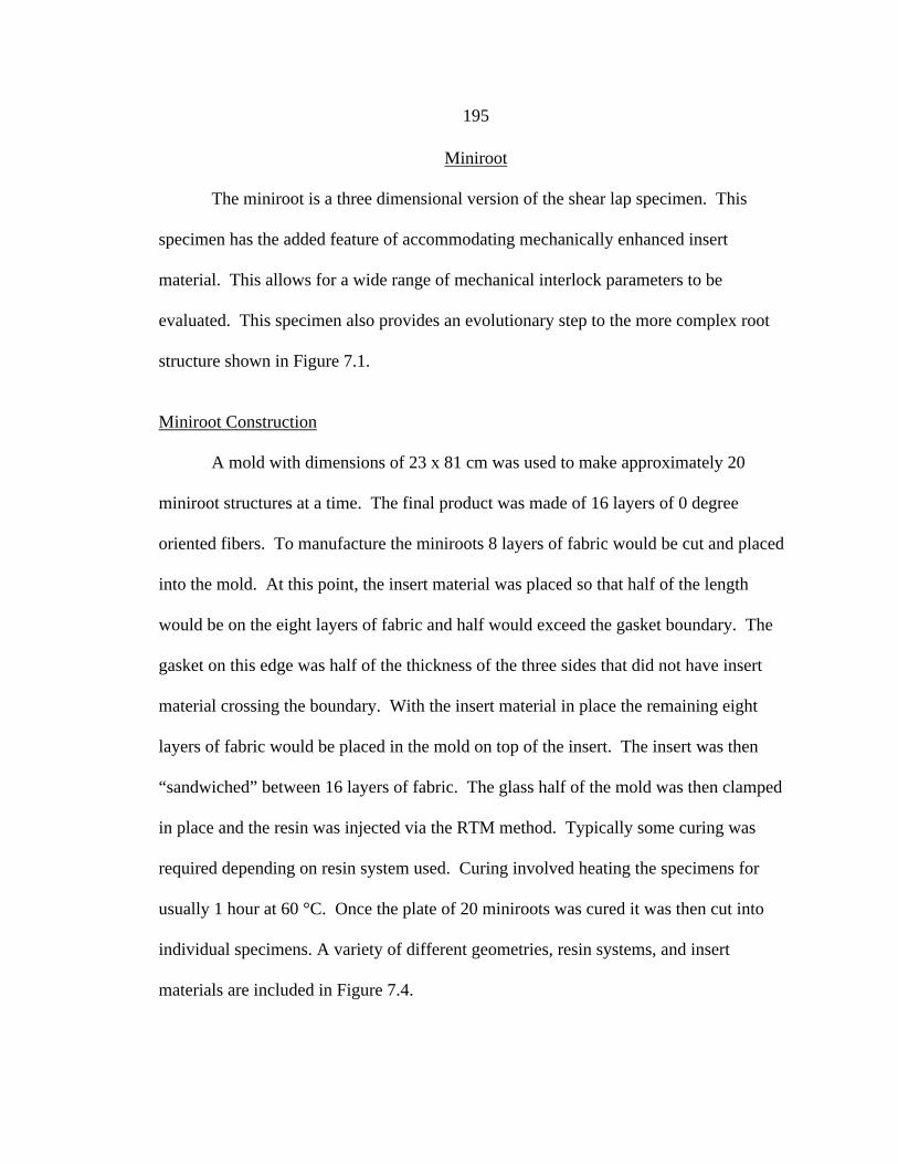
195
Miniroot
The miniroot is a three dimensional version of the shear lap specimen. This
specimen has the added feature of accommodating mechanically enhanced insert
material. This allows for a wide range of mechanical interlock parameters to be
evaluated. This specimen also provides an evolutionary step to the more complex root
structure shown in Figure 7.1.
Miniroot Construction
A mold with dimensions of 23 x 81 cm was used to make approximately 20
miniroot structures at a time. The final product was made of 16 layers of 0 degree
oriented fibers. To manufacture the miniroots 8 layers of fabric would be cut and placed
into the mold. At this point, the insert material was placed so that half of the length
would be on the eight layers of fabric and half would exceed the gasket boundary. The
gasket on this edge was half of the thickness of the three sides that did not have insert
material crossing the boundary. With the insert material in place the remaining eight
layers of fabric would be placed in the mold on top of the insert. The insert was then
“sandwiched” between 16 layers of fabric. The glass half of the mold was then clamped
in place and the resin was injected via the RTM method. Typically some curing was
required depending on resin system used. Curing involved heating the specimens for
usually 1 hour at 60 °C. Once the plate of 20 miniroots was cured it was then cut into
individual specimens. A variety of different geometries, resin systems, and insert
materials are included in Figure 7.4.
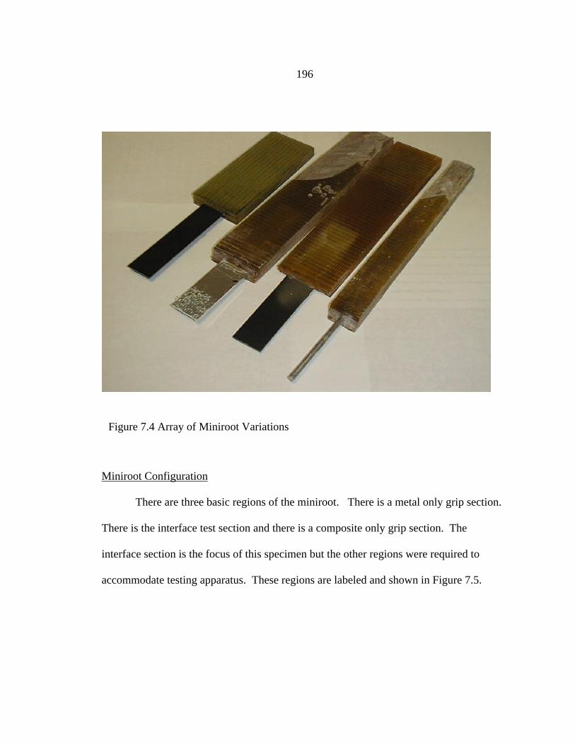
196
Miniroot Configuration
There are three basic regions of the miniroot. There is a metal only grip section.
There is the interface test section and there is a composite only grip section. The
interface section is the focus of this specimen but the other regions were required to
accommodate testing apparatus. These regions are labeled and shown in Figure 7.5.
Figure 7.4 Array of Miniroot Variations
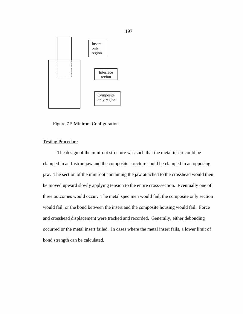
197
Testing Procedure
The design of the miniroot structure was such that the metal insert could be
clamped in an Instron jaw and the composite structure could be clamped in an opposing
jaw. The section of the miniroot containing the jaw attached to the crosshead would then
be moved upward slowly applying tension to the entire cross-section. Eventually one of
three outcomes would occur. The metal specimen would fail; the composite only section
would fail; or the bond between the insert and the composite housing would fail. Force
and crosshead displacement were tracked and recorded. Generally, either debonding
occurred or the metal insert failed. In cases where the metal insert fails, a lower limit of
bond strength can be calculated.
Insertonlyregion
Interfaceregion
Compositeonly region
Figure 7.5 Miniroot Configuration
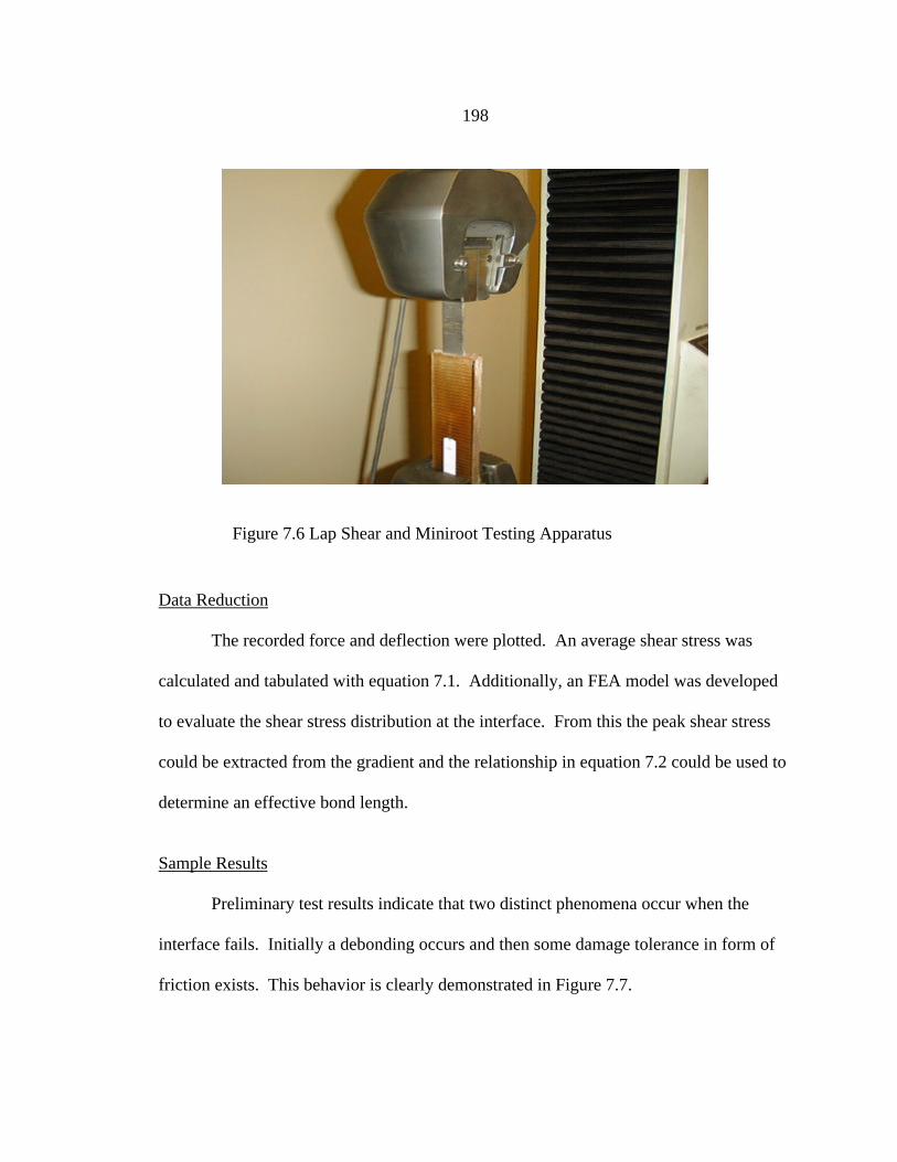
198
Data Reduction
The recorded force and deflection were plotted. An average shear stress was
calculated and tabulated with equation 7.1. Additionally, an FEA model was developed
to evaluate the shear stress distribution at the interface. From this the peak shear stress
could be extracted from the gradient and the relationship in equation 7.2 could be used to
determine an effective bond length.
Sample Results
Preliminary test results indicate that two distinct phenomena occur when the
interface fails. Initially a debonding occurs and then some damage tolerance in form of
friction exists. This behavior is clearly demonstrated in Figure 7.7.
Figure 7.6 Lap Shear and Miniroot Testing Apparatus
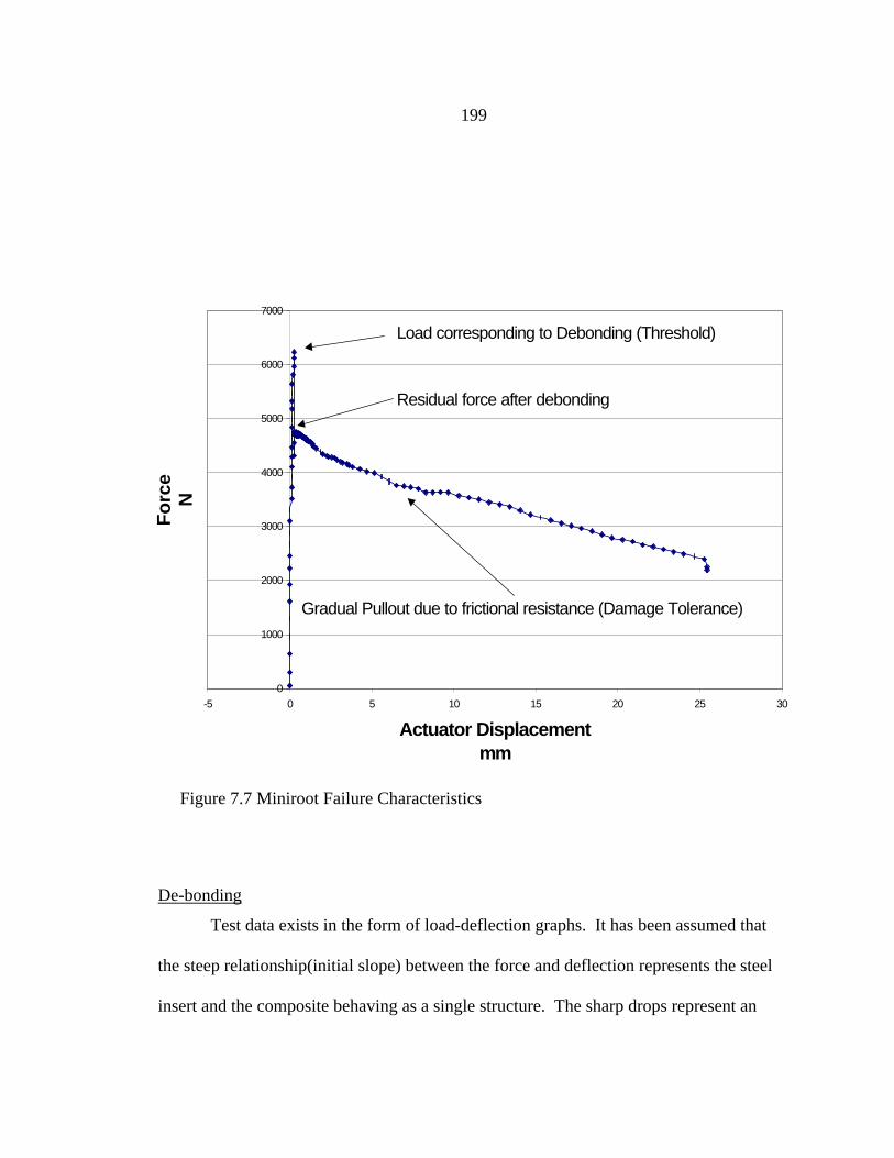
199
De-bonding
Test data exists in the form of load-deflection graphs. It has been assumed that
the steep relationship(initial slope) between the force and deflection represents the steel
insert and the composite behaving as a single structure. The sharp drops represent an
0
1000
2000
3000
4000
5000
6000
7000
-5 0 5 10 15 20 25 30
Actuator Displacementmm
Fo
rce
N
Load corresponding to Debonding (Threshold)
Residual force after debonding
Gradual Pullout due to frictional resistance (Damage Tolerance)
Figure 7.7 Miniroot Failure Characteristics
200
increase in compliance and a subsequent de-bonding of the metal insert from the
composite casing. Ideally this threshold load associated with de-bonding should be
resolved into a failing stress. Most likely the miniroot structure’s interface is failing from
shear stress. This is the mechanism most likely transferring load from the insert to the
composite.
Pull-out
Once the bond between the resin material and the insert has broken the curve
levels off and the load gradually drops off. Damage tolerance exists in the form of
friction. Residual stresses create tractions and forces normal to the insert surface, which
induce this friction. The tractions responsible for this friction are either from differing
elastic properties or residual stresses from curing process, which involves a 40 °C
temperature gradient.
Metal Interface Experimental Results
The three specimen described earlier were constructed and tested based on
methods outlined. The single lap shear, double lap shear, and miniroot test results will be
discussed on an individual basis. The shear lap specimen were used to evaluate chemical
bond capabilities, while the miniroot specimen were an evolutionary step used to evaluate
mechanical bond capabilities.
Parametric Study
Three different resin systems were used to construct several different SLS, DLS.
and miniroot structures. Other variatons included surface treatment, insert or lap
201
material, and structural alterations. These parameter that were investigated will be briefly
discussed as well as the test matrix and specific experimental results.
Surface Treatment
The surface treatment greatly affects the bond characteristics of metals. Chemical
alterations in form of etchents can increase bond strength. Phosphoric acid was used for
steel and ASTM D 2651-90.was followed for aluminum. Mechanical conditioning, such
as sanding and bead blasting increases bond strength as well. Additionally the bond
surface can be tapped, knurled, or modified by other machining processes to enhance the
structural bond.
Elastic Properties
The elastic properties of the composite affect load sharing. These properties such
as shear modulus, Poisson’s ratio, and Young’s modulus determine the manner in which
the force and related stresses are distributed through the material. The magnitude of the
interfacial stresses and the associated gradient are strictly a function of the material
properties and the miniroot dimensions.
Chemical Bond Characteristics
As stated earlier, the miniroot’s ability to with stand loading is based on chemical
bond and structural bond characteristics or properties. Each resin system has a unique
molecular structure. Vinylesters are different than Polyesters, which vary from Epoxies
in molecular structure. Each different type of resin system and particular resin has
different bondability with the metals.
202
Mechanical Bond Characteristics
Measures were taken to improve the overall bond strength by increasing the
mechanical bond directly. Alterations were made to the insert surface to enhance the
mechanical interlock between the composite and the insert metal. A variety of
modifications were made. Ideally each progression of mechanical bond improvement
would approach the aggressive root structure.
1. Plain
2. Knurled
3. Threaded
Knurling
This surface treatment was applied to the round specimens only due to ease of
machining. Three different patterns were applied. A straight or longitudinal groove was
used as well as a criss-cross or diamond pattern similar to a typical knurled handle.
Threading
In addition to knurling, threading was also applied to some specimens. The
threads were applied with a simple tap. The threaded specimens provided and
evolutionary step from the simple miniroot structure to the complex root structure.
Resin Systems
Three candidate resin systems were used to construct the shearlap and miniroot
test specimens. The polyester 63-AX-051 system is an unsaturated, orthophthalic
polyester manufactured by Interplastics corporation. Extensive research has been
203
conducted on this system by DOE/MSU research effort. Due to the abundance of the
information available on this system, it was chosen as a baseline [Orozco (1999)].
Another improved version of the above resin system was the isopthalic polyester resin.
The vinylester 8084 system is a rubber toughened epoxy vinylester provided by Dow
Chemical. This system has shown better performance with regard to fracture toughness
and tensile strength compared to the baseline polyester [Orozco (1999)].
Layup Variations
When measures were taken to improve the mechanical interlock between the
composite housing and the metal insert, the fiber orientation can play an important role.
Orienting the fibers in 45 degree manner could allow an improved interlock between the
fibers and the machined insert. The layers of fabric adjacent to the insert were varied in
orientation to evaluate the affect of fabric interlock.
Insert Material
The elastic properties and dimensions of the insert material also affect the manner
in which load is shared and distributed. The insert materials used in this study were
isotropic. The major difference in varying the insert material was the elastic modulus.
Steel also has different bond characteristics than aluminum. The insert material can
affect both the chemical bond as well as the load sharing properties.
Insert Coating
To provide a reduced shear transition between the insert material and the
composite housing material, the inserts were sometimes coated with an epoxy material.
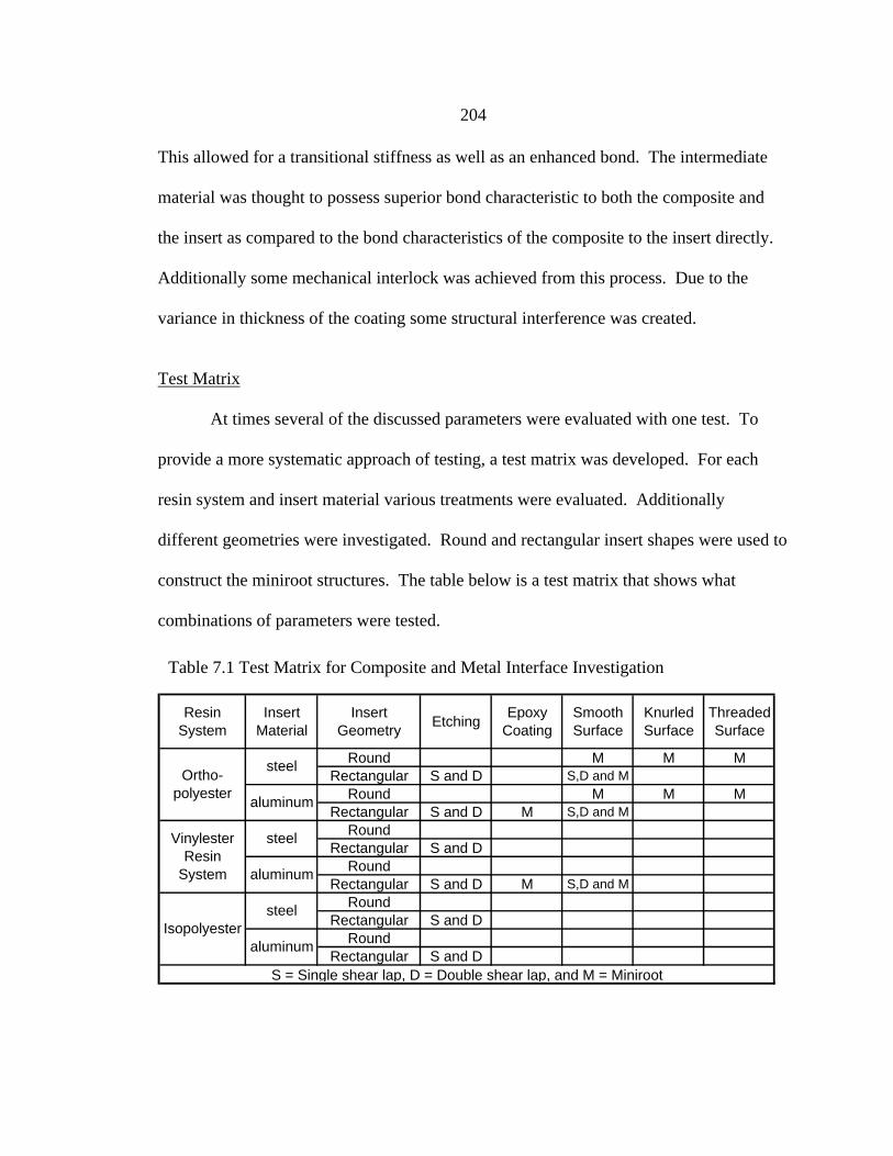
204
This allowed for a transitional stiffness as well as an enhanced bond. The intermediate
material was thought to possess superior bond characteristic to both the composite and
the insert as compared to the bond characteristics of the composite to the insert directly.
Additionally some mechanical interlock was achieved from this process. Due to the
variance in thickness of the coating some structural interference was created.
Test Matrix
At times several of the discussed parameters were evaluated with one test. To
provide a more systematic approach of testing, a test matrix was developed. For each
resin system and insert material various treatments were evaluated. Additionally
different geometries were investigated. Round and rectangular insert shapes were used to
construct the miniroot structures. The table below is a test matrix that shows what
combinations of parameters were tested.
Resin System
Insert Material
Insert Geometry
EtchingEpoxy
CoatingSmooth Surface
Knurled Surface
Threaded Surface
Round M M MRectangular S and D S,D and M
Round M M MRectangular S and D M S,D and M
RoundRectangular S and D
RoundRectangular S and D M S,D and M
RoundRectangular S and D
RoundRectangular S and D
Ortho-polyester
Vinylester Resin
System
Isopolyester
steel
aluminum
steel
aluminum
steel
aluminum
S = Single shear lap, D = Double shear lap, and M = Miniroot
Table 7.1 Test Matrix for Composite and Metal Interface Investigation

205
Single Lap Shear (SLS) Experimental Results
Single lap shear specimens were constructed of aluminum and steel adherend
material. The adhesive or resin was one of three resins investigated. An orthopolyester
was used as a baseline to compare to an isopolyester and a toughened vinylester. A test
matrix shown in Table 7.1 displays the combination of materials tested. The adherends
were also prepared with an industry accepted etchant to enhance the bond strength. The
SLS samples were then compared to un-etched samples for both metal adherends for all
three resin systems. Generally 6 specimen were tested, in some cases there were less.
Each specimen was tested as described. The failing or peak load was recorded
and used for data reduction. The experimental strength was based on the failing load and
total bond area (equation 7.1). It has been suggested that the length of the bond does not
contribute to the strength as much as the width of the bond due to the shear stress
gradient [Skeist (1977) and Hart-Smith (1990)]. As a result the failing load was also
divided by the width only. The results for both data reduction techniques are included.
The load per area results and the load per unit width results are shown in Table 7.2 and
7.3 respectively.
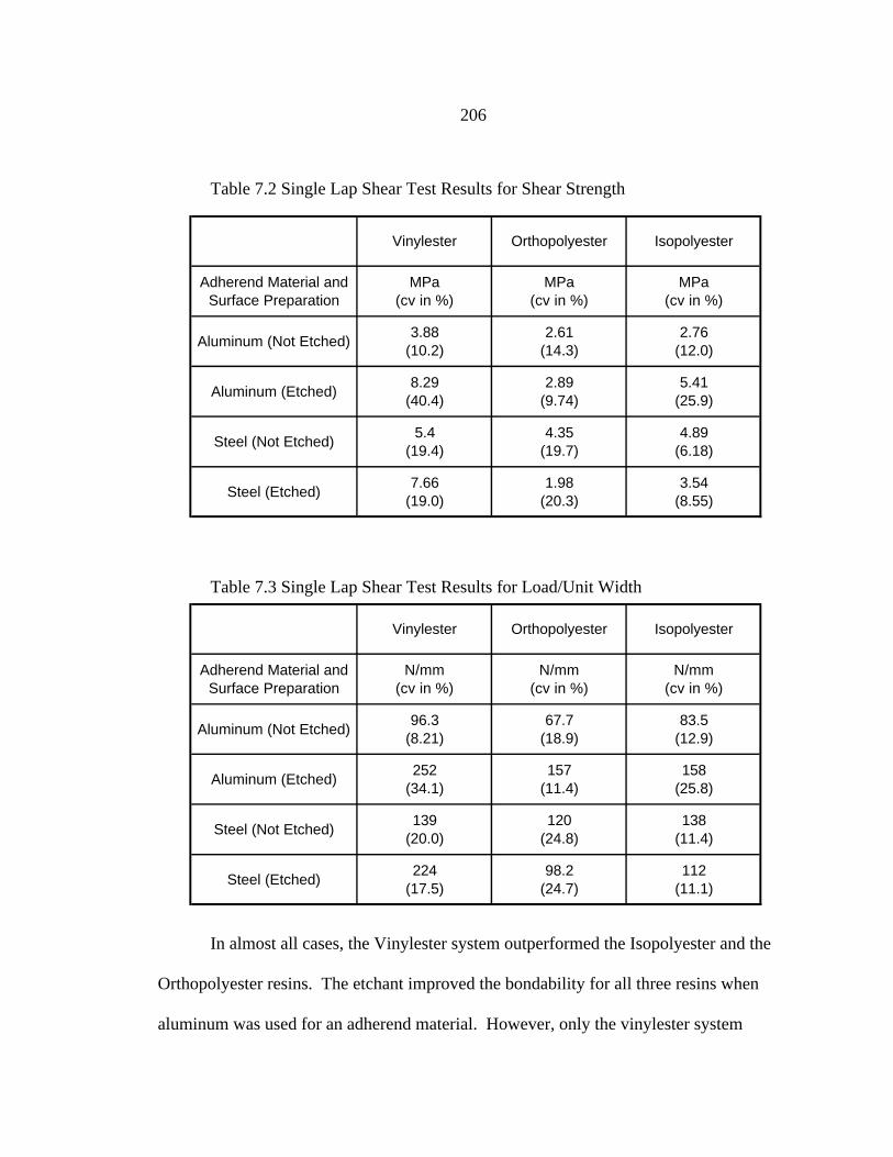
206
In almost all cases, the Vinylester system outperformed the Isopolyester and the
Orthopolyester resins. The etchant improved the bondability for all three resins when
aluminum was used for an adherend material. However, only the vinylester system
Table 7.3 Single Lap Shear Test Results for Load/Unit Width
Vinylester Orthopolyester Isopolyester
Adherend Material and Surface Preparation
N/mm (cv in %)
N/mm (cv in %)
N/mm (cv in %)
Aluminum (Not Etched)96.3
(8.21)67.7
(18.9)83.5
(12.9)
Aluminum (Etched)252
(34.1)157
(11.4)158
(25.8)
Steel (Not Etched)139
(20.0)120
(24.8)138
(11.4)
Steel (Etched)224
(17.5)98.2
(24.7)112
(11.1)
Table 7.2 Single Lap Shear Test Results for Shear Strength
Vinylester Orthopolyester Isopolyester
Adherend Material and Surface Preparation
MPa (cv in %)
MPa (cv in %)
MPa (cv in %)
Aluminum (Not Etched)3.88
(10.2)2.61
(14.3)2.76
(12.0)
Aluminum (Etched)8.29
(40.4)2.89
(9.74)5.41
(25.9)
Steel (Not Etched)5.4
(19.4)4.35
(19.7)4.89
(6.18)
Steel (Etched)7.66
(19.0)1.98
(20.3)3.54
(8.55)

207
showed an improvement from etching for the steel adherend SLS samples. The (load per
unit width) results generally follow the shear strength results. Both indicate that steel
bonded better than aluminum when no etchents were used. When etchents were used the
aluminum SLS specimen exceeded the steel. The load per area results and the load per
unit width results compared closely. Since the bond length was consistent the either
metric would probably be adequate.
Double Lap Shear (DLS) Experimental Results
The DLS specimen was very similar to the SLS specimen. The primary
difference is that the DLS specimen is more symmetric and is less likely to effected by
bending. As a result the DLS test results are expected to be a better representation of the
upper limit of the bond capabilities. As with the SLS specimens the Double Lap Shear
(DLS) specimens were constructed of two different metal adherends and bonded with
three different resins. This was done for etched and non-etched variations. A test matrix
is provided in Table 7.1 and the test results are shown in Table 7.4.
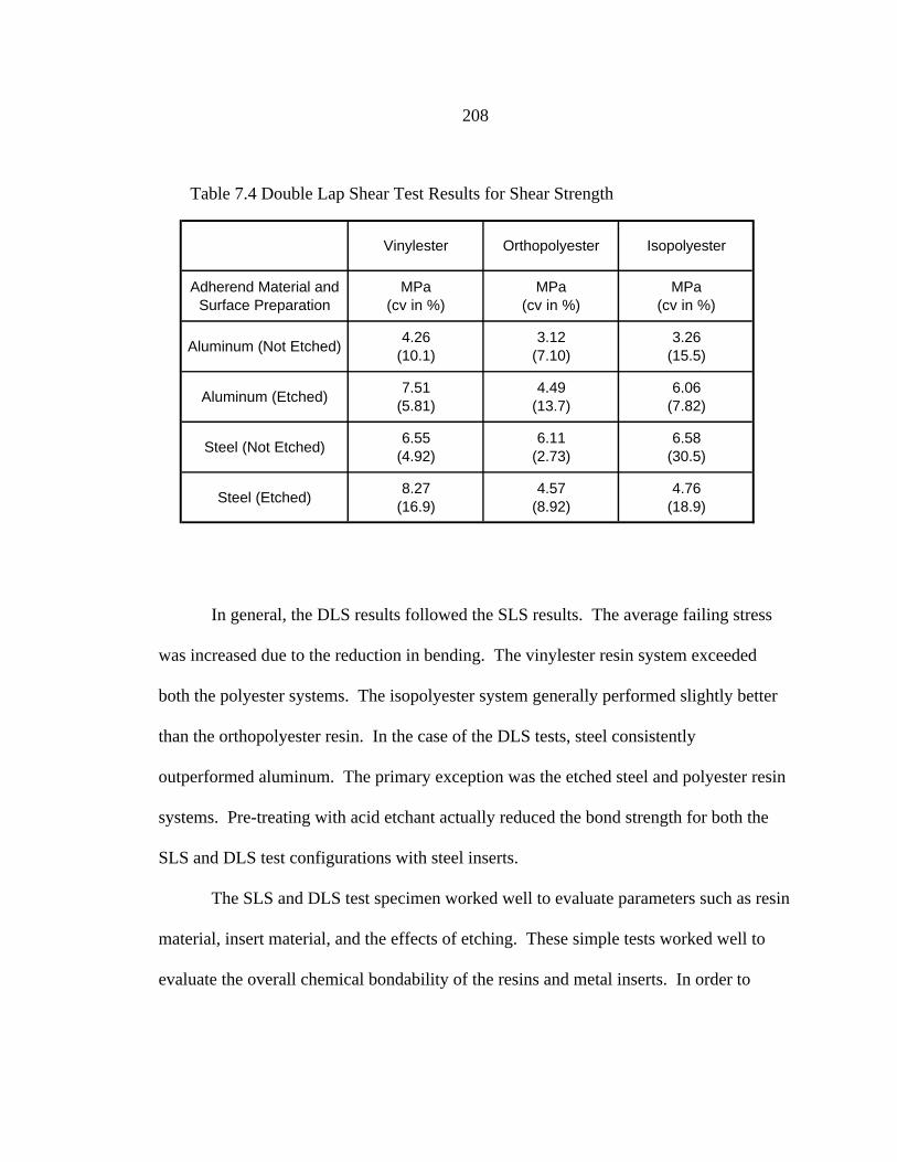
208
In general, the DLS results followed the SLS results. The average failing stress
was increased due to the reduction in bending. The vinylester resin system exceeded
both the polyester systems. The isopolyester system generally performed slightly better
than the orthopolyester resin. In the case of the DLS tests, steel consistently
outperformed aluminum. The primary exception was the etched steel and polyester resin
systems. Pre-treating with acid etchant actually reduced the bond strength for both the
SLS and DLS test configurations with steel inserts.
The SLS and DLS test specimen worked well to evaluate parameters such as resin
material, insert material, and the effects of etching. These simple tests worked well to
evaluate the overall chemical bondability of the resins and metal inserts. In order to
Table 7.4 Double Lap Shear Test Results for Shear Strength
Vinylester Orthopolyester Isopolyester
Adherend Material and Surface Preparation
MPa (cv in %)
MPa (cv in %)
MPa (cv in %)
Aluminum (Not Etched)4.26
(10.1)3.12
(7.10)3.26
(15.5)
Aluminum (Etched)7.51
(5.81)4.49
(13.7)6.06
(7.82)
Steel (Not Etched)6.55
(4.92)6.11
(2.73)6.58
(30.5)
Steel (Etched)8.27
(16.9)4.57
(8.92)4.76
(18.9)

209
investigate the mechanical effects of various degrees of interlock, the miniroot test was
required.
Miniroot Experimental Results
Several interesting comparisons were made with this unique test specimen. The
miniroot test configuration accommodated such variations as insert shape, intermediate
adhesive coatings, and various levels of mechanical interlock. These parameters will be
discussed individually.
Insert Coating Effects
As stated, it was expected that using an intermediate bond material might enhance
the overall bond strength. A standard Devcon produced epoxy adhesive was applied to
the surface of the metal inserts. This adhesive coating was allowed to dry and the entire
insert was placed in the composite layup based on the miniroot construction procedure.
This was done with aluminum inserts and two resin systems. For both the polyester and
vinylester systems controls were also tested that were not coated with the epoxy material.
The established testing procedure was used to apply force until the specimen debonded
or some type of failure occurred. In cases of debond the force was applied after failure to
capture the damage tolerance of the bond. Graphical representation of this is shown in
Figure 7.8.
Figure 7.8 Effects of Using an Epoxy Coating as an Intermediate Adhesive Layer
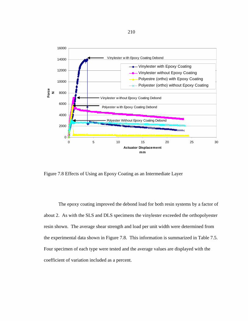
210
0
2000
4000
6000
8000
10000
12000
14000
16000
0 5 10 15 20 25 30
Actuator Displacement mm
Fo
rce
N
Vinylester with Epoxy Coating
Vinylester without Epoxy Coating
Polyestre (ortho) with Epoxy Coating
Polyester (ortho) without Epoxy Coating
Vinylester w ith Epoxy Coating Debond
Vinylester w ithout Epoxy Coating Debond
Polyester w ith Epoxy Coating Debond
Polyester Without Epoxy Coating Debond
Figure 7.8 Effects of Using an Epoxy Coating as an Intermediate Layer
The epoxy coating improved the debond load for both resin systems by a factor of
about 2. As with the SLS and DLS specimens the vinylester exceeded the orthopolyester
resin shown. The average shear strength and load per unit width were determined from
the experimental data shown in Figure 7.8. This information is summarized in Table 7.5.
Four specimen of each type were tested and the average values are displayed with the
coefficient of variation included as a percent.
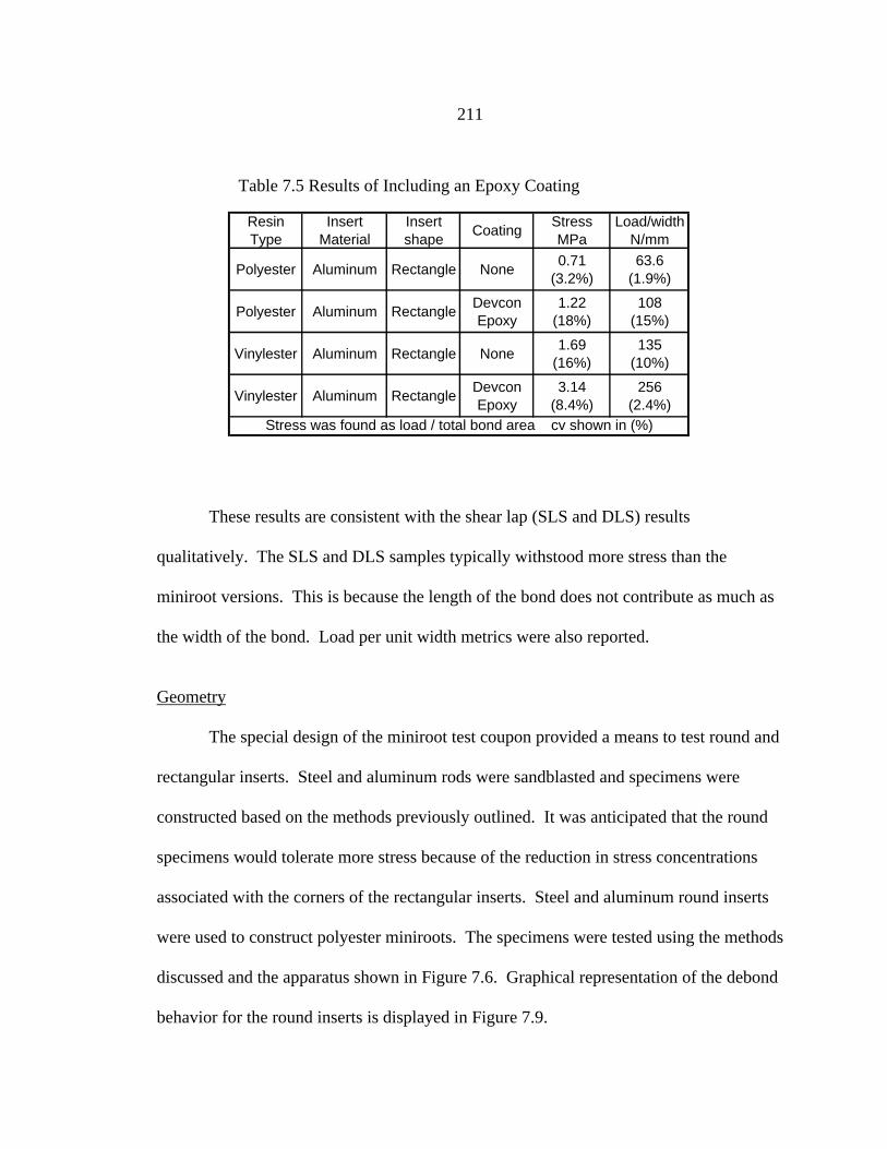
211
These results are consistent with the shear lap (SLS and DLS) results
qualitatively. The SLS and DLS samples typically withstood more stress than the
miniroot versions. This is because the length of the bond does not contribute as much as
the width of the bond. Load per unit width metrics were also reported.
Geometry
The special design of the miniroot test coupon provided a means to test round and
rectangular inserts. Steel and aluminum rods were sandblasted and specimens were
constructed based on the methods previously outlined. It was anticipated that the round
specimens would tolerate more stress because of the reduction in stress concentrations
associated with the corners of the rectangular inserts. Steel and aluminum round inserts
were used to construct polyester miniroots. The specimens were tested using the methods
discussed and the apparatus shown in Figure 7.6. Graphical representation of the debond
behavior for the round inserts is displayed in Figure 7.9.
Resin Type
Insert Material
Insert shape
CoatingStress MPa
Load/width N/mm
Polyester Aluminum Rectangle None0.71
(3.2%)63.6
(1.9%)
Polyester Aluminum RectangleDevcon Epoxy
1.22 (18%)
108 (15%)
Vinylester Aluminum Rectangle None1.69
(16%)135
(10%)
Vinylester Aluminum RectangleDevcon Epoxy
3.14 (8.4%)
256 (2.4%)
Stress was found as load / total bond area cv shown in (%)
Table 7.5 Results of Including an Epoxy Coating
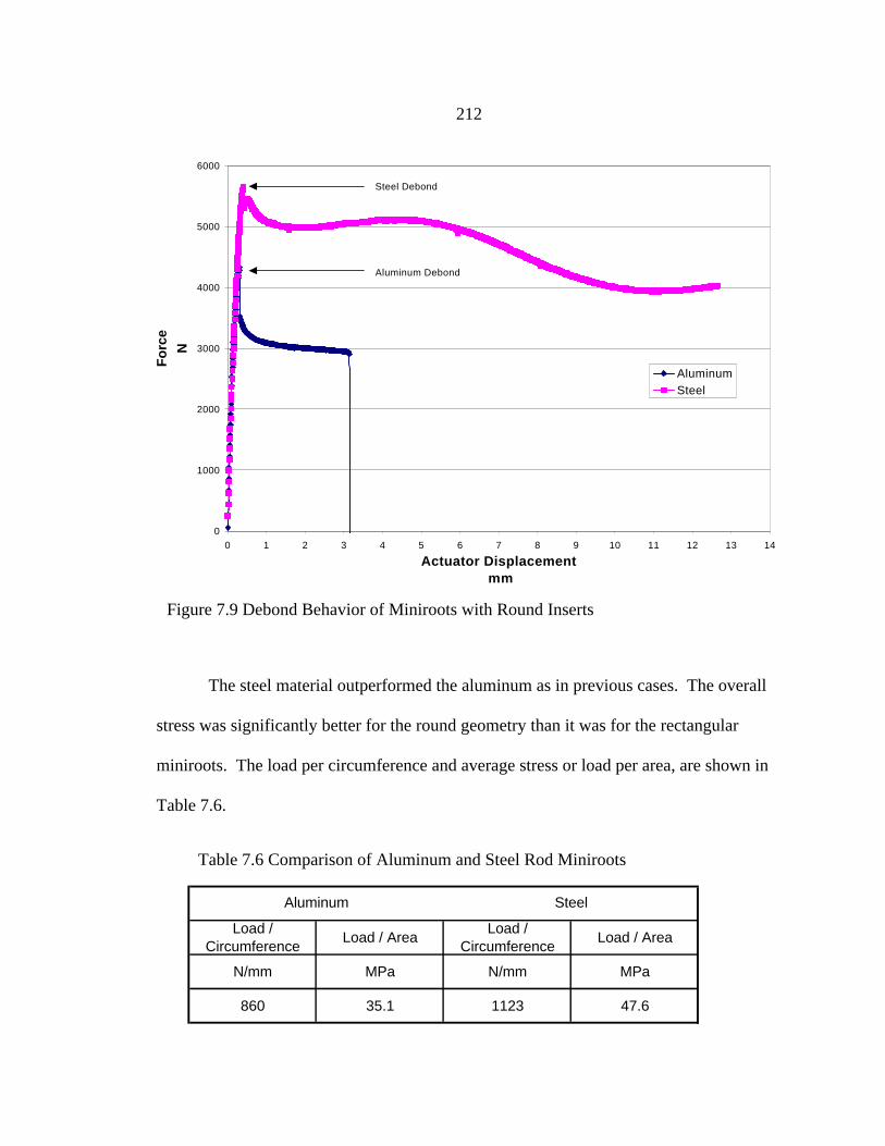
212
The steel material outperformed the aluminum as in previous cases. The overall
stress was significantly better for the round geometry than it was for the rectangular
miniroots. The load per circumference and average stress or load per area, are shown in
Table 7.6.
0
1000
2000
3000
4000
5000
6000
0 1 2 3 4 5 6 7 8 9 10 11 12 13 14
Actuator Displacement mm
Fo
rce
N
AluminumSteel
Aluminum Debond
Steel Debond
Figure 7.9 Debond Behavior of Miniroots with Round Inserts
Load / Circumference
Load / AreaLoad /
CircumferenceLoad / Area
N/mm MPa N/mm MPa
860 35.1 1123 47.6
Aluminum Steel
Table 7.6 Comparison of Aluminum and Steel Rod Miniroots
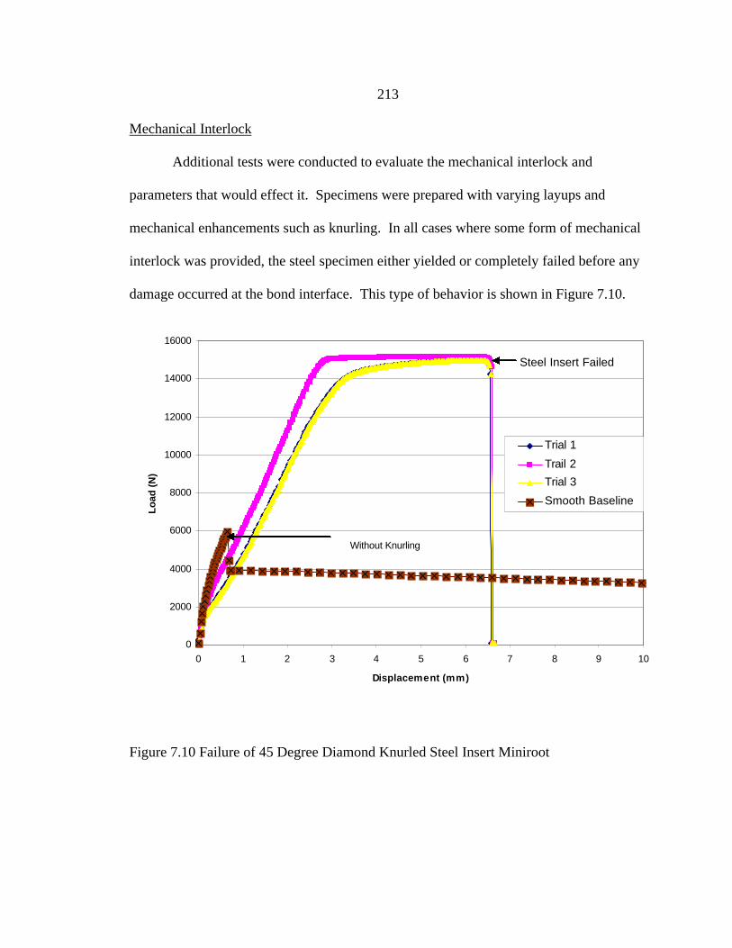
213
Mechanical Interlock
Additional tests were conducted to evaluate the mechanical interlock and
parameters that would effect it. Specimens were prepared with varying layups and
mechanical enhancements such as knurling. In all cases where some form of mechanical
interlock was provided, the steel specimen either yielded or completely failed before any
damage occurred at the bond interface. This type of behavior is shown in Figure 7.10.
0
2000
4000
6000
8000
10000
12000
14000
16000
0 1 2 3 4 5 6 7 8 9 10
Displacement (mm)
Lo
ad (
N)
Trial 1
Trail 2
Trial 3
Smooth Baseline
Steel Insert Failed
Without Knurling
Figure 7.10 Failure of 45 Degree Diamond Knurled Steel Insert Miniroot
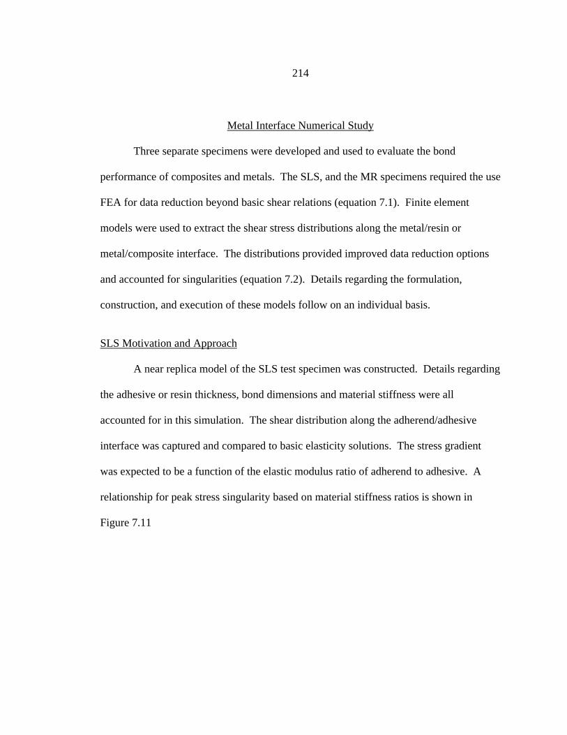
214
Metal Interface Numerical Study
Three separate specimens were developed and used to evaluate the bond
performance of composites and metals. The SLS, and the MR specimens required the use
FEA for data reduction beyond basic shear relations (equation 7.1). Finite element
models were used to extract the shear stress distributions along the metal/resin or
metal/composite interface. The distributions provided improved data reduction options
and accounted for singularities (equation 7.2). Details regarding the formulation,
construction, and execution of these models follow on an individual basis.
SLS Motivation and Approach
A near replica model of the SLS test specimen was constructed. Details regarding
the adhesive or resin thickness, bond dimensions and material stiffness were all
accounted for in this simulation. The shear distribution along the adherend/adhesive
interface was captured and compared to basic elasticity solutions. The stress gradient
was expected to be a function of the elastic modulus ratio of adherend to adhesive. A
relationship for peak stress singularity based on material stiffness ratios is shown in
Figure 7.11
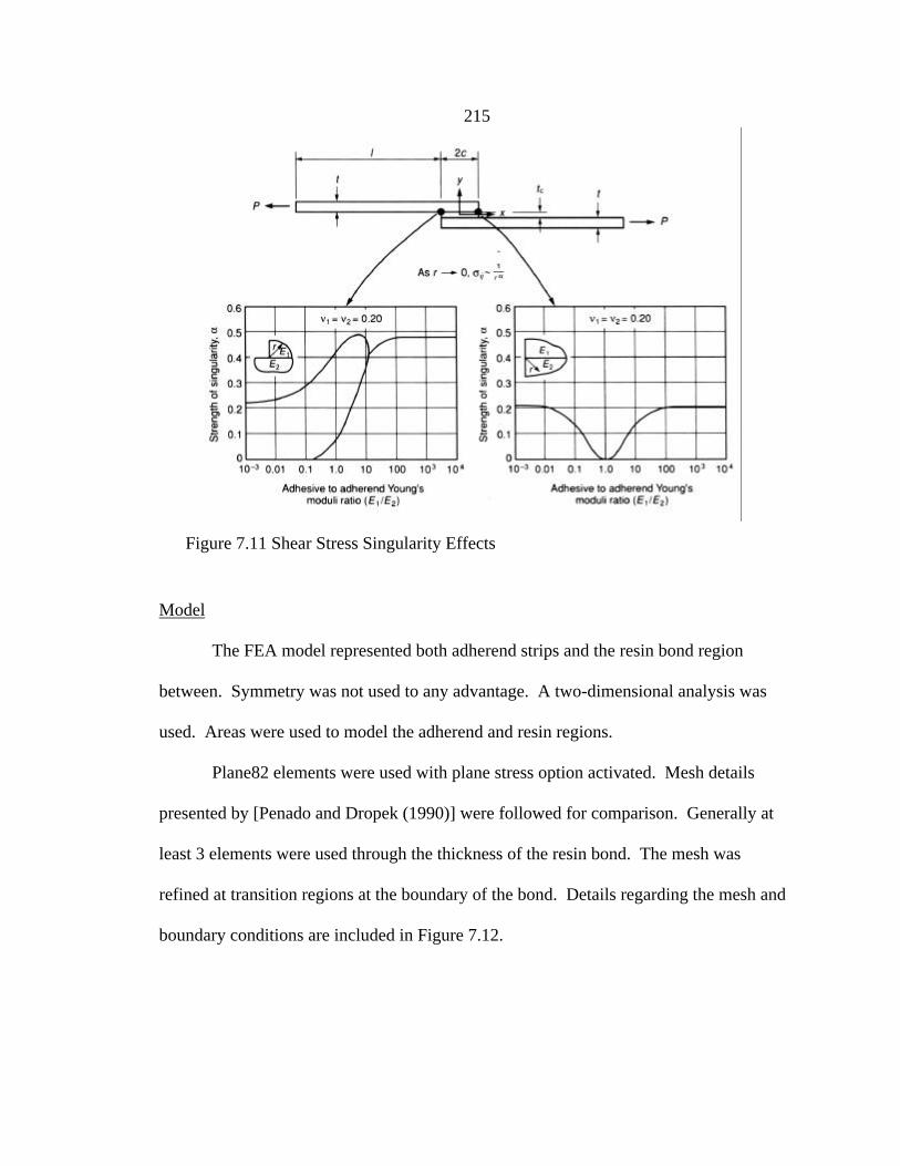
215
Model
The FEA model represented both adherend strips and the resin bond region
between. Symmetry was not used to any advantage. A two-dimensional analysis was
used. Areas were used to model the adherend and resin regions.
Plane82 elements were used with plane stress option activated. Mesh details
presented by [Penado and Dropek (1990)] were followed for comparison. Generally at
least 3 elements were used through the thickness of the resin bond. The mesh was
refined at transition regions at the boundary of the bond. Details regarding the mesh and
boundary conditions are included in Figure 7.12.
Figure 7.11 Shear Stress Singularity Effects
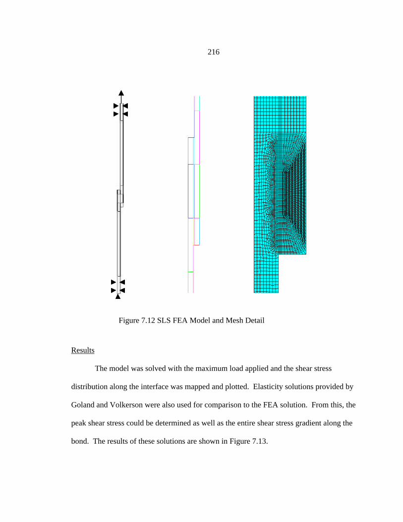
216
Results
The model was solved with the maximum load applied and the shear stress
distribution along the interface was mapped and plotted. Elasticity solutions provided by
Goland and Volkerson were also used for comparison to the FEA solution. From this, the
peak shear stress could be determined as well as the entire shear stress gradient along the
bond. The results of these solutions are shown in Figure 7.13.
Figure 7.12 SLS FEA Model and Mesh Detail
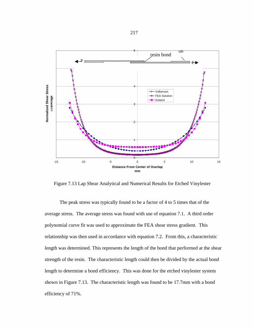
217
The peak stress was typically found to be a factor of 4 to 5 times that of the
average stress. The average stress was found with use of equation 7.1. A third order
polynomial curve fit was used to approximate the FEA shear stress gradient. This
relationship was then used in accordance with equation 7.2. From this, a characteristic
length was determined. This represents the length of the bond that performed at the shear
strength of the resin. The characteristic length could then be divided by the actual bond
length to determine a bond efficiency. This was done for the etched vinylester system
shown in Figure 7.13. The characteristic length was found to be 17.7mm with a bond
efficiency of 71%.
0
1
2
3
4
5
6
-15 -10 -5 0 5 10 15
Distance From Center of Overlapmm
No
rmal
ized
Sh
ear
Str
ess
τ/τ
τ/τa
vera
ge
Volkerson
FEA Solution
Goland
tabresin bond
PP
Figure 7.13 Lap Shear Analytical and Numerical Results for Etched Vinylester
218
Miniroot Motivation and Approach
It was known that there would be definite affects of the miniroot’s structure on the
behavior of the bond. It was assumed that a shear stress gradient between the composite
surface and the insert surface was responsible for the debonding of the insert.
Experimentally the debond load was resolved into a bond strength by dividing the force
by the penetrated surface area. However it was suspect that a uniform stress state did not
exist, as was shown by the lap shear results.
To better assess the material behavior and to develop a means to quantify the
bond strength, FEA was implemented. The intent was to capture the stress behavior at
the interface and ultimately use the model to explain this behavior and possibly predict
performance.
Model
The ANSYS code was used to evaluate all test cases. A macro was developed to
generate geometry, mesh elements, constrain and load the miniroot structure. Brick
(solid 45) elements were used to compose a full 3-D model for the De-bonding model.
Quarter symmetry was utilized to reduce the number of elements required. Several
solutions were obtained with differing meshes, order of element, and geometry. Initially
16,880 elements were required for this model. This provided 1mm x 1mm elements
which corresponded to 5 elements through the thickness for the composite and 1 element
through the thickness for the steel insert. The model was resolved with a solid 95 element
to test convergence. That second solution verified the original.
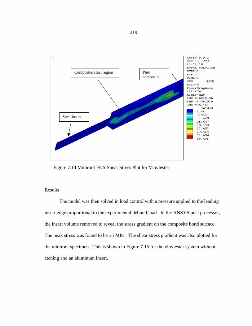
219
Results
The model was then solved in load control with a pressure applied to the leading
insert edge proportional to the experimental debond load. In the ANSYS post processor,
the insert volume removed to reveal the stress gradient on the composite bond surface.
The peak stress was found to be 35 MPa. The shear stress gradient was also plotted for
the miniroot specimen. This is shown in Figure 7.15 for the vinylester system without
etching and an aluminum insert.
Figure 7.14 Miniroot FEA Shear Stress Plot for Vinylester
Composite/Steel region Purecomposite
Steel insert
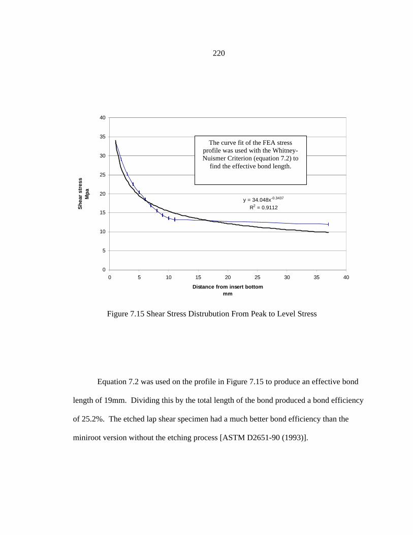
220
Equation 7.2 was used on the profile in Figure 7.15 to produce an effective bond
length of 19mm. Dividing this by the total length of the bond produced a bond efficiency
of 25.2%. The etched lap shear specimen had a much better bond efficiency than the
miniroot version without the etching process [ASTM D2651-90 (1993)].
y = 34.048x-0.3437
R2 = 0.9112
0
5
10
15
20
25
30
35
40
0 5 10 15 20 25 30 35 40
Distance from insert bottommm
Sh
ear
stre
ssM
pa
Whitney - Nuesemmer Plot to Findshear stress distribution frommaximum peak
Power (Whitney - Nuesemmer Plotto Find shear stress distribution frommaximum peak)
Figure 7.15 Shear Stress Distrubution From Peak to Level Stress
The curve fit of the FEA stressprofile was used with the Whitney-Nuismer Criterion (equation 7.2) to
find the effective bond length.
221
Summary for Case Study IV
The data base-screening approach was applied to this case study. The primary
goal was to develop a series of tests that could be used to test various parameters that
relate to the bond performance of composite and metal interfaces. An additional goal of
this study was to determine if the bond performance could be quantified as a material
property and used as an analytical design tool. A special evolution of test specimen and
testing procedures were developed to evaluate the performance of metal to composite
bond interfaces.
Unique data reduction techniques were employed to characterize and quantify the
bond performance. In general, the length of the interfacial bond contributes less to the
strength than does the width of the bond. As a result experimental load limits were
compared to overall bond area as well as bond width. Another hypothesis was that a
peak stress singularity might be a consistent limit for bonds of the type investigated. A
final method of reduction investigated was the Whitney-Nuismer Criterion. This
approach determines an effective bond efficiency based on a stress distribution extracted
from a finite element analysis.
At the onset of the project these four techniques were to be applied at each level
of test geometry (single shear lap, double shear lap, and miniroot specimen). Potentially,
a technique that showed promise could be extended to root test specimen and ultimately
to a blade design detail.
From the experimental test results obtained and the applied data reduction
techniques, no clear quantity proved to be repeatable at all levels of geometry

222
development. A primary problem with the testing conducted was that the metal
adherends were routinely the limiting factor of the test specimen evaluated. Even in the
case of the single and double shear lap specimen the bond typically would not fail until
the metal insert began to yield and contract away from the bond. Similar behavior was
observed for the smooth rectangular miniroots. For the mechanically interlocked
versions of the miniroot, the insert material always failed completely before the bond
would break. This behavior is consistent at the full-size root level also.
The screening process experimentally provided useful qualitative results. It was
found that etching the adherends improved the chemical bond characteristics
significantly. Additionally, the intermediate epoxy coating improved the chemical bond
strength by a factor of almost 2. The vinylester resin system exceeded the polyester
competitors for bond strength. The screening shear lap test used worked well to
investigate these modifications quickly and affordably.
This investigation reinforces the need to test composite structures and materials
substantially. The behavior of the bond failures was predictable but, the load levels could
not presently be predicted.

223
CHAPTER 8
CONCLUSIONS AND FUTURE WORK
A general methodology was developed to quantify the interlaminar fracture
toughness of composite materials. Four separate case studies were investigated to help
establish and validate the approach. The approach consisted of two distinct paths. An
analytical approach that employed the use of FEA and basic G (strain energy release rate)
properties was investigated as well as a screening approach that compared candidate
composites at a material level and other subsequent stages of structural development.
Ideally, some blend of these two options is most desirable. It was found that substantial
experimental validation is required to establish confidence in FEA models. Occasionally
FEA was required for basic data reduction and experimental interpretation when the
analytical approach was abandoned. The experimental (screening) approach and the FEA
analytical approach were very complementary. Neither approach uniquely quantifies the
complex behavior of composites. The database-screening approach proved worthy
for every project and required limited resources.
This chapter contains conclusive results from each case study that can generally
be applied to other topics and projects. Additionally, a structured approach to composite
design is offered. The majority of the conclusions and suggestions are related to
screening processes and their importance to composite material design.

224
Composite Material Design Process
1. Apply analytical methods available to evaluate forces and stresses on
component desired. With intended use of structure known, evaluate design
drivers and potential weaknesses.
2. With the aid of classical lamination theory, develop an architecture scheme
that best addresses the above critical loading scenario. Details such as fiber
type, resin system, fiber volume, and fiber orientation should be decided at
this stage. Other criteria should also be met, such as glass transition
temperature, environmental affects of moisture, and other material properties
that were not addressed by this study.
3. With ideal architecture candidates formed, the initial construction of simple
plates should be conducted. Specimens can be sampled from these plates
which can then be subjected to tensile testing, mode I fracture testing, static
flexure testing, etc…
4. Empirical methods should be applied to test data to evaluate basic strength
and fracture toughness properties. Damage should be inspected to assess the
limitation of the materials performance. Empirical testing of these plates
should provide important estimates of material properties. Knowing these
properties will be important, because these will need to be implemented into
FEA models or used with other means to predict and avoid structural failure.
225
Rival materials can be compared at this point. This serves as a screening
process. The materials that show the most promise at the completion of step 4
should then be developed into desired geometry or structure. FEA Models of
test specimens should be developed to confirm testing results. These models
can eventually evolve to predict the behavior of complex structures that will
be made from the composite materials.
5. Iterate and adjust parameters to refine and improve the overall performance of
the composite material.
6. Construct actual part or component. Some intermediate testing and screening
may be necessary.
Importance of the Screening Process
Fracture mechanics as applied to composites is not an exact science. It is difficult
to first assess fracture related material properties, and to second use them as a predictive
tool in design. Using the test and analysis methods outlined can serve as an effective
approach to compare candidate materials at a developmental level. The material
properties obtained from this methodology could then be used with the FEA techniques
presented to predict damage or failure in simple structures.
Case Study Review
Case study I and case study II were material property investigations that resulted
from full-scale failures. At the point of failure, little was known about the actual
properties of the materials used. Additionally, limited structural analysis had been
conducted with regard to the final product.
226
The developmental screening process provided both of these sponsors with a
means to compare simple composite architecture alternatives. It also would have
provided them with important material properties to use for failure analysis.
Case study III was a good example of a classic application. Even in cases where
initial attempts are successful, a screening process has value. In case study IV the root
structure developed was performing satisfactorily. However, there were several unknown
parameters. Limited iterations were made to arrive at the successful root structure.
Improving on this design required some backtracking and down scaling.
Case Study I Composite Aerofan Blade Evaluation
• Excessive through thickness reinforcement of composite architectures
sacrifices in plane properties to unacceptable levels.
• Through thickness reinforcement significantly increases fracture toughness.
Some optimized percentage of cross-stitching could provide an ideal blend of
delamination resistance and necessary in plane properties.
• Most of the reinforced material behaved in a bilinear fashion. Ideally, an
Aerofan blade should maintain crisp linearity up to threshold. This is because
in the event of a collision, blade survival and engine survival would be greatly
reduced due to an unbalanced deformed semi-damaged blade.
• The 5 series material possessed the most impressive static and dynamic
flexure strength of 845 MPa and 745 MPa respectively. MSU produced
materials have rivaled this performance with equal or greater fracture
toughness. Some investigation should be conducted with other resin systems,
227
because possibly the difficult processing requirements of PR 520 may be
inhibiting bonding performance or other process events.
Case Study II X-33 Fuel Tank Investigation
• The usage of sandwich theory to increase stiffness and strength introduces a
bond layer. This bond layer possesses some fracture toughness but still may
limit the overall performance of the material.
• The lobe 1 replacement material performed better in all regards except
transverse compression. This exception was most likely related to the aspect
ratio of the specimens. The compression test was effectively a critical
buckling analysis. The interfacial bond was improved for lobe 1 to the point
that core failure occurred during mode I, and transverse tension testing.
• GII values were typically a factor of 10 larger than the GI values. This might
indicate that any fracture type failure would most likely be mode I. However
this depends greatly on the loading, not just the fracture resistance. It should
be noted that some shear was present during mode I testing due to the
geometry of the test specimen this was observed and confirmed with the aid of
FEA analysis.
• Foam reinforcement material outperformed the honeycomb core. Foam
splices were able to detour cracks from the core into the facesheet.
• Employing these testing techniques could have prolonged the X33 space
program since its ultimate limitation was the honeycomb fuel tanks.

228
Case Study III Aerospace Composite Resin Characterization
• Strength properties were not necessarily proportional or inversely proportional
to interlaminar properties. This requires a dedicated assessment or testing to
characterize the composite’s fracture toughness.
• Mode I performance did not always follow Mode II.
• Impact testing provided a means to evaluate strain rate sensitivity as it relates
to interlaminar fracture.
• Relationship between laminate microstructure and interlaminar fracture
observed with SEM technology.
Case Study IV Metal Interface Evaluation
• Simple tests provided the most results.
• FEA worked well for data reduction and aided in the overall understanding of
the load sharing behavior.
• The evolution of tests developed worked well.

229
Future Recommendations
The scope of this study was broad, and several of the details investigated could be
further pursued. These details as well as the global focus of interlaminar fracture
characterization will be discussed.
In general, the screening process developed was sensible and simple. The
mentality and methodology associated with the process could be extended to other design
issues relating to composite materials. Ideally, a generalized design process needs to be
established that addresses strength, stiffness, interlaminar fracture, environmental
conditions, and fatigue considerations of composite materials. This process could then be
applied to optimize a potential composite candidate material.
To implement the screening approach of comparison, design drivers and
limitations need to be identified. Pertinent material properties that are related to intended
performance can be acquired through subsequent testing. The acquired material
properties can be used as a material database for analysis. Analysis can be closed form
mathematical solutions, empirical formulas, or finite element codes. Ultimately the
analysis can be used as a design tool to minimize expensive testing and construction
iterations. The FEA methods presented could be used to avoid interlaminar fracture in
damage tolerant structures. However, the current technology needs to be advanced and
further validated with examples like those in Case study I and II.
230
REFERENCES CITED
ANSYS (1998). “Engineering Analysis System”, (10thed) Canonsburg, PA: ANSYS Inc.
ASM V19 (1997) “Fatigue and Fracture” ASM International, Materials Park, OH.
ASTM C 297-94 (1997). “Standard Test Method for Flatwise Tensile Strength ofSandwich Constructions, C 297-94”, 1997 Annual Book of ASTM Standards, Vol15.03, 1997, pp.9-10.
ASTM C 365-94 (1997). “Standard Test Method for Flatwise Compressive Propertiesof Sandwich Cores, C 365-94”, 1997 Annual Book of ASTM Standards, Vol15.03, 1997, pp.15-17.
ASTM C 393-94 (1997). “Standard Test Method for Flexural Properties of SandwichConstructions, C 393-94”, 1997 Annual Book of ASTM Standards, Vol 15.03,1997, pp.21-26.
ASTM D 1002-72 (1993). “Standard Test Method for Strength Properties of Adhesivesin Shear by Tension Loading (Metal to Metal), D 1002-72”, 1993 Annual Book ofASTM Standards, Vol 15.06, 1993, pp.47-49.
ASTM D 2651-90 (1993). “Standard Guide for Preparation of Metal Surfaces forAdhesive Bonding, D 2651 – 90”, 1993 Annual Book of ASTM Standards, Vol15.06, 1993, pp.170-174.
ASTM D 3983-92 (1993). “Standard Test Method for Measuring Strength and ShearModulus of Nonrigid Adhesives by the Thick-Adherend Tensile-Lap Specimen, D3983-92”, 1993 Annual Book of ASTM Standards, Vol 15.06, 1993, pp.309-317.
ASTM D 4027-92 (1993). “Standard Test Method for Measuring Shear Properties ofStructural Adhesives by the Modified-Rail Test, D 4027-92”,1993 Annual Bookof ASTM Standards, Vol 15.06, 1993, pp.319-332.
ASTM D 4562-90 (1993). “Standard Test Method for Shear Strength of AdhesivesUsing Pin-and-Collar Specimen, D 4562-90”, 1993 Annual Book of ASTMStandards Vol 15.06, 1993, pp.378-380.
ASTM D 4896-89 (1993). “Standard Guide for Use of Adhesive-Bonded Single Lap-Joint Specimen Test Results D 4896 - 89”, 1993 Annual Book of ASTMStandards, Vol 15.06, 1993, pp.419-423.
231
ASTM D 5528-94a (1997). “Standard Test Method for Mode I Interlaminar FractureToughness of Unidirectional Fiber-Reinforced Polymer Matrix Composites, D5528 – 94a”, 1997 Annual Book of ASTM Standards, Vol. 15.03, 1997, pp.271-279.
ASTM E 229-92 (1993). “Standard Test Method for Shear Strength and Shear Modulusof Structural Adhesives, E 229-92”, 1993 Annual Book of ASTM Standards, Vol15.06, 1993, pp.454-458.
ASTM E 399-90 (1992). “Standard Test Method for Plane-Strain Fracture Toughness ofMetallic Materials, E 399 – 90”, 1992 Annual Book of ASTM Standards, Vol.15.03, 1997, pp.509-539.
ASTM E 813-89 (1991). “Standard Test Method for JIc, A Measure of FractureToughness, E 399-90,” 1991 Annual Book of ASTM Standards, Vol. 03.01, 1991,pp. 738-752.
Astrom, B.T., (1997) “Manufacturing of Polymer Composites”. 1st ed. London,England: Chapman & Hall.
Broek, D. (1996). “Elementary Engineering Fracture Mechanics” (4th edition). Boston,Massachusetts: Kluwer Academic Publishers.
Cairns, D.S., (1999) “Personal Interview,” Montana State University-Bozeman,Bozeman, Montana.
Cairns, D.S., (1992) “Static and Dynamic Mode II Strain Energy Release Rates inToughened Thermosetting Composite Laminates,” ASTM Journal of CompositesTechnology & Research, Volume 14, No. 1, Spring 1992, pp. 37-42.
Cairns, D.S. (1990) “Mechanisms of Fracture and Toughening in Multiphase Materials,”22nd International SAMPE Technical Conference, November 6-8, 1990.
Cairns, D.S. and Lagace, P. A. (1992) “A Consistent Engineering Methodology for theTreatment of Impact in Composite Materials,” Journal of Reinforced Plastics andComposites, Vol. 11 April 1992, pp. 395-412.
Carlsson, L.A. (1991) “On the Design of the Cracked Sandwich Beam (CSB)Specimen,” Journal of Reinforced Plastics and Composites, Volume 10, July1991, pp. 434-443.
Carlsson, L.A., Sendlein, L.S., and Merry, S.L., (1986) “Characterization of FaceSheet/Core Shear Fracture of Composite Sandwich Beams,” Journal of CompositeMaterials, 25(1)” 101-116.
232
Carlsson, L.A.,Gillespie, L.A., and Pipes, R.B., (1986) “On the Analysis and Design ofthe End Notch Flexure Specimen (ENF) specimen for mode II testing,” Journal ofComposite Materials, Volume 20, November 1986, pp. 594-603.
Freitas, G. and Fusco,T., (1995) “Z-Fiber Technology and Products for EnhancingComposite Design,” Waltham, MA: Aztec Inc.
Gere, J.M.and Timoshenko, S.P. (1984). “Mechanics of Materials” (3rd edition). Boston,MA: PWS-KENT Publishing Co.
Gillespie, J.W.,Carlsson, L.A., and Pipes, R.B., (1986) “Finite Element Analysis of theEnd Notch Flexure Specimen for Measuring Mode II Fracture Toughness,”Composites Science and Technology, Volume 27, pp.177-197.
Griffith A.A., (1920). “Philos. Trans. R. Soc.” Vol. A221, London, England, p.163.
Hart-Smith, L.J. (1990). “Rating and Comparing Structural Adhesives: A New Method”Engineering Materials Handbook(Adhesives and Sealants) Vol 3, 1990, pp.471-476.
Haugen D. (1998). “Fracture of Skin Stiffener Intersections in Composite WindTurbine Blade Structures” Master’s Thesis, Montana State University-Bozeman,Bozeman MT.
Hyer, M. W. (1998). “Stress Analysis of Fiber Reinforced Composite Materials”. Boston, Massachusetts: McGraw-Hill.
HPC (2000). “X-33 Update (Experimental Composite Tanks)” High PerformanceComposites, Volume 8 number 1, Jan/Feb 2000, page 9.
HPC (2001). “X-33 Update (Composite Tanks to be Replaced with Aluminum)” HighPerformance Composites, Volume 9 number 1, Jan/Feb 2001, page 15.
Irwin, G.R. (1949). “Fracturing of Metals, American Society for Metals,” Cleveland.Ohio. pp. 146 – 148.
Jarmon, D.C., Weeks, C.A., Naik, R.A., Kogstrom, C.L., Logan, C.P., and Braun, P.F.(1998). “Mechanical Property Comparison of 3-D and 2-D Graphite ReinforcedEpoxy Composites Fabricated by RTM,” 43rd International SAMPESymposium/Exhibition.
Jones, R. M. (1999). “Mechanics of Composite Materials” (2nd edition). Leviitown, PA:Taylor and Francis.
233
Mackin, T.J., (1992) “A Comparison of Instrumented Impact Testing and GardnerImpact Testing,” Santa Barbara, CA: Dynatup Products Division GeneralResearch Corp.
Mandell J.F., and Samborsky D.D. (1997). DOE/MSU composite material fatiguedatabase: Test methods, materials, and analysis (Contractor Report No.SAND97,3002). Albuquerque, NM: Sandia National Laboratories.
McMichael, S., and Fischer, S., (1989) “Understanding Materials with InstrumentedImpact,” Santa Barbara, CA Dynatup Products Division. General Research Corp.
Morehead, R.B. (2000). “Fatigue of Skin Stiffener Intersections in Composite WindTurbine Blade Structures” Master’s Thesis, Montana State University-Bozeman,Bozeman MT.
Naik, R.A. Jarmon, D.C., Weeks, C.A., and Logan, C.P. (1998). “Characterization andModeling of Advanced Architecture Woven Materials,” 43rd InternationalSAMPE Symposium/Exhibition.
Norton, R. L. (1996). “Machine Design (An Integrated Approach)”. Upper Saddle River,NJ: Prentice Hall.
Orozco, R. (1999). “Effects of Toughened Matrix Resins on Composite Materials forWind Turbine Blades” Master’s Thesis, Montana State University-Bozeman,Bozeman MT.
Penado, F.E. and Dropek, R.K. (1990). “Numerical Design and Analysis”, EngineeringMaterials Handbook(Adhesives and Sealants) Vol 3, 1990, pp.477-500.
Russel, A.J. and Street, K.N. (1987). “The Effect of Matrix Toughness on Delamination:Static and Fatigue Fracture Under Mode II Shear Loading of Graphite FiberComposites,” Toughened Composites, ASTM STP 937, ASTM, Philadelphia,PA. pp 275.
Rybicki, E.F. and Kanninen, M.F. (1977). “A Finite Element Calculation of StressIntensity Factors by a Modified Crack Closure Integral,” Engineering FractureMechanics, Vol. 9, 1977, pp. 931-938.
Skeist, I. (1977). “Handbook of Adhesives” (2nd Ed). Livingston, NJ: Van NostrandReinhold Company.
234
Skramstad, J.D. (1999). “Evaluation of hand lay-up and resin transfer molding incomposite wind turbine blade manufacturing”, Master’s Thesis, Montana StateUniversity-Bozeman, Bozeman MT.
Sun, T.C. (1997). “Calculation of Stress Intensity Factors for Interlaminar Cracks in Composite Laminates,” Composites Science and Technology, Vol. 57, 1997,pp 637-650.
Tsai, S.W. (1971). A General Theory of Strength for Anisotropic Materials, J.Composite Materials, January, 1971, pp. 58-80.
Tsai, S.W. (1988). Composite Design 4th edition, Think Composites. Dayton, OH.
Valisetty, R.R. and Chamis, C.C. (1988). “Sublaminate or Ply-Level Analysis ofComposites and Strain Energy Release Rates of End-Notch and Mixed-ModeFracture Specimens,”Composite Materials: Testing and Design(8th conference),ASTM STP 972, ASTM, Philadelphia, Pennsylvania, pp. 41-56.
Weeks, C.A., Naik, R.A., and Kogstrom, C.L. (1998). “Analysis of Damage in ThroughThickness Reinforced Composites Induced by Soft Body Impact,” 43rd
International SAMPE Symposium/Exhibition.
Whitney, J.M. and Nuismer, R.J. (1974). “Stress Fracture Criteria for LaminatesContaining Stress Concentrations,” Journal of Composites, vol. 8, pp. 253-265.

235
APPENDIX A
FINITE ELEMENT CODES

236
Static Flexure FEA Macro
/PREP7!This Model Constructs a representation of a basic 3-pt Bending Apparatus!and Static Flexure Specimen. Symmetry is employed at the midplane!The effects of friction due to the testing fixture are also captured
!Initial Dimensions of Test Geometry
!Specimenhalfspan=63.5thick=6.135overhang=22
!Support Fixturerad=9.50sloprad=9.70
!Keypoints to Construct SpecimenK,1,0,0,0K,2,overhang,0,0K,3,halfspan+overhang,0,0K,4,halfspan+overhang,thick,0K,5,0,thick,0
!Lines Required to Construct SpecimenLSTR,1,2LSTR,2,3LSTR,3,4LSTR,4,5LSTR,5,1
!Area Representing SpecimenAL,1,2,3,4,5
!Element DeclarationET,1,PLANE 82KEYOPT,1,3,3R,1,25.4
!Material PropertiesMP,EX,1,74.5E3MP,PRXY,1,.3
237
!Element SizingESIZE,thick/6
!Meshing of SpecimenTYPE,1MAT,1AMESH,1
!Stability and Symmetry Boundary ConditionDL,3,1,UX,0
!Steel Properties for FixtureMP,EX,2,209E3MP,PRXY,2,.3
!Roller GenerationCYL4,OVERHANG,-RAD,RAD
!Roller MeshingMSHAPE,1,2DMSHKEY,0TYPE,1MAT,2AMESH,2
!Construction of Fixture Using KeypointsK,22,OVERHANG-SLOPRAD,-RAD,0K,23,OVERHANG+SLOPRAD,-RAD,0K,24,OVERHANG+25.4,-RAD,0K,25,OVERHANG-25.4,-RAD,0K,26,OVERHANG,-RAD,0K,27,OVERHANG-25.4,-35.1,0K,28,OVERHANG+25.4,-35.1,0
!Lines from KeypointsLARC,22,23,9LSTR,22,25LSTR, 23,24
LSTR,25,27LSTR,27,28

238
LSTR,28,24
!Area from LinesAL,10,11,13,14,15,12
!Meshing of FixtureMSHAPE,1,2DMSHKEY,0TYPE,1MAT,2AMESH,3
!Application of Jig constraintsDA,3,ALL,0
!The contact wizard should then be employed to produce!2 flexible-flexible 2-D contact pairs or surfaces!One between the roller and fixture and the other between the roller and sample
!Apply Load to Specimen Center and Solve

239
ENF FEA Macro
/PREP7!This Model is a Representation of the ENF Test Specimen
!Specimen DimensionsSUPPORT=11CRACK=39L=171T=6.135
!Construction of Keypoints for GeometryK,1,0,0,0K,2,L,0,0K,3,L,T/3,0K,4,4/3*CRACK,T/3,0K,5,CRACK,T/3,0K,6,0,T/3,0K,7,L,2*T/3,0K,8,4/3*CRACK,2*T/3,0K,9,CRACK,2*T/3,0K,10,0,2*T/3,0K,11,0,T/2,0K,12,CRACK,T/2,0K,13,L,T,0K,14,0,T,0K,15,0,T/2,0K,16,SUPPORT,T/3,0K,17,SUPPORT,T/2,0K,18,SUPPORT,2*T/3,0K,19,SUPPORT,T/2,0K,20,4/3*CRACK,T/2,0
!Construction of Areas From KeypointsA,6,16,17,11A,16,5,12,17A,19,12,9,18A,15,19,18,10A,5,4,20,12A,12,20,8,9
A,4,3,7,8A,1,2,3,4,5,16,6A,10,18,9,8,7,13,14

240
!Declaration of Element TypeET,1,PLANE 82KEYOPT,1,3,3R,1,1
!Assignment of Material PropertiesMP,EX,1,75E3MP,PRXY,1,.3
!MeshingESIZE,.5TYPE,1MAT,1AMESH,5AMESH,6AMESH,3AMESH,2
ESIZE,1TYPE,1MAT,1AMESH,1AMESH,4
ESIZE,1TYPE,1MAT,1AMESH,7AMESH,8AMESH,9
!Use Contact Wizard to Generate Contact Surfaces on the Lines that Form the Crack!Apply Y Constraints at the Roller Locations and an X Constraint at the Node with the!Critical Load and Solve

241
Flatwise Tension FEA Macro
/PREP7!FEA Model of Flat Wise Tension Specimens!TOL variable allows for the shifting of the steel tabs!FWT properties determined from test scraps.!Flexure used to Assess face sheet properties!Assumed modulus from FWT experiment used for core material
!The model can be ran with different values of TOL!Geometric Parameters for Face Sheet and Core Thicknesses and Specimen Width
WIDTH=37T1=1.6T2=37T3=4TTOTAL=T1+T2+T3
!Geometric Parameters for Steel Fixture or TabFLANGE=4WEBT=4HEIGHT=29TOL=0
!Declaration of Element SizeESIZE,1
!KeypointsK,1,0,0,0K,2,WIDTH,0,OK,3,WIDTH,T1,OK,4,0,T1,OK,5,0,T1+T2,0K,6,WIDTH,T1+T2,0K,7,WIDTH,T1+T2+T3,0K,8,0,T1+T2+T3,0
!Generating Areas from KeypointsA,1,2,3,4A,3,4,5,6A,5,6,7,8
!Assignment of Material Core PropertiesMP,EX,1,21

242
MP,PRXY,1,.3
!Assignment of MaterialMP,EX,2,43400MP,PRXY,2,.3
!Declaration of Element TypeET,1,PLANE 82KEYOPT,1,3,3R,1,37
!Meshing of Core RegionTYPE,1MAT,1AMESH,2
!Meshing of Face SheetsTYPE,1MAT,2AMESH,1AMESH,3
!Construction of Steel TabsK,9,0,-FLANGE,0K,10,WIDTH/2-WEBT/2+TOL,-FLANGE,0K,11,WIDTH/2-WEBT/2+TOL,-HEIGHT,0K,12,WIDTH/2+WEBT/2+TOL,-HEIGHT,0K,13,WIDTH/2+WEBT/2+TOL,-FLANGE,0K,14,WIDTH,-FLANGE,0
A,1,2,14,13,12,11,10,9
K,15,0,FLANGE+TTOTAL,0K,16,WIDTH/2-WEBT/2,FLANGE+TTOTAL,0K,17,WIDTH/2-WEBT/2,HEIGHT+TTOTAL,0K,18,WIDTH/2+WEBT/2,HEIGHT+TTOTAL,0K,19,WIDTH/2+WEBT/2,FLANGE+TTOTAL,0K,20,WIDTH,FLANGE+TTOTAL,0
A,7,8,15,16,17,18,19,20
!Material Properties for SteelMP,EX,3,200000

243
MP,PRXY,3,.3
Meshing of Steel TabsTYPE,1MAT,3AMESH,4AMESH,5
!Constrain center node at bottom with DN,UX,0 and DN,UY,0!Where N is the node number.!Constrain center node at top iwth DN,UX,0!Apply Appropriate Force to Top Node.!Solve
!Use Map Function to Map Membrane stress to x location and extract for plots

244
DCB Specimen FEA Macro
/PREP7!This Model Represents the DCB Sandwich Panel Test Specimen
!Specimen Dimensions!L=Length, C=Crack length, W=width, T1,T2, and T3 are face sheet and core thicknessesL=150C=50T1=4T2=37T3=1.64W=37.5
!Creation of Keypoints for GeometryK,1,0,0,0K,2,L,0,0K,3,L,T1,0K,4,0,T1,0K,5,L,T1+T2-T3,0K,6,4/3*C,T1+T2-T3,0K,7,C,T1+T2-T3,0K,8,0,T1+T2-T3,0K,9,L,T1+T2,0K,10,4/3*C,T1+T2,0K,11,C,T1+T2,0K,12,0,T1+T2,0K,13,L,T1+T2+T3,0K,14,4/3*C,T1+T2+T3,0K,15,C,T1+T2+T3,0K,16,0,T1+T2+T3,0K,17,0,T1+T2,0
!Creation of Areas from KeypointsA,1,2,3,4A,4,3,5,6,7,8A,8,7,11,12A,7,6,10,11A,6,5,9,10A,10,9,13,14A,11,10,14,15A,17,11,15,16

245
!Declaration of element typeET,1,PLANE 82KEYOPT,1,3,3R,1,W
!Material Properties!Elastic ModulusMP,EX,1,42200MP,PRXY,1,.3MP,EX,2,50MP,PRXY,2,.3
!Declaration of Element Size and MeshingESIZE,.2TYPE,1MAT,1AMESH,8AMESH,7
TYPE,1MAT,2AMESH,3AMESH,4
ESIZE,2TYPE,1MAT,1AMESH,6AMESH,1
TYPE,1MAT,2AMESH,5
ESIZE,6TYPE,1MAT,2AMESH,2
!Restrain x and y displacement at node corresponding to hinge location at bottom!Restrain x displacement at node corresponding to hinge location at top!Apply critical load and solve
246
Shear Lap Specimen FEA Macro
/PREP7!This model replicates the Shear lap specimen
!Shear Lap Specimen Properties!TM = Metal thickness, TR = Resin thickness, LR = Length of the bond, LM Length ofMetal.TM=1.43TR=.070LR=29LM=150GRIP=25
!Keypoints for GeometryK,1,0,0,0K,2,TM,0,0K,3,TM,LM-5/4*LR,0K,4,0,LM-5/4*LR,0K,5,TM,LM-3/4*LR,0K,6,0,LM-3/4*LR,0K,7,TM,LM-LR/4,0K,8,0,LM-LR/4,OK,9,TM,LM,0K,10,0,LM,0K,11,TM,LM-LR,0K,12,TM+TR,LM-LR,0K,13,TM+TR,LM-3/4*LR,0K,14,TM+TR,LM-LR/4,0K,15,TM+TR,LM,0K,16,2*TM+TR,LM-LR,0K,17,2*TM+TR,LM-3*LR/4,0K,18,2*TM+TR,LM-LR/4,0K,19,2*TM+TR,LM+LR/4,0K,20,2*TM+TR,2*LM-LR,0K,21,TM+TR,2*LM-LR,0K,22,TM+TR,LM+LR/4,0K,23,TM,GRIP,0K,24,0,GRIP,0K,25,TM+TR,2*LM-LR-GRIP,0K,26,2*TM+TR,2*LM-LR-GRIP,0
!Creating Areas from KeypointsA,1,2,23,24

247
A,24,23,3,4A,4,3,11,5,6A,6,5,7,8A,8,7,9,10
A,11,12,13,5A,5,13,14,7A,7,14,15,9
A,12,16,17,13A,13,17,18,14A,14,18,19,22,15A,19,26,25,22A,25,26,20,21
!Assignment of Material PropertiesMP,EX,2,200000MP,PRXY,2,.3MP,EX,1,3250MP,PRXY,1,.35
!Element DeclarationET,1,PLANE82ESIZE,TR/3
!Meshing of Resin RegionTYPE,1MAT,1AMESH,6AMESH,8
ESIZE,TM/8TYPE,1MAT,1AMESH,7
!Meshing of SteelTYPE,1MAT,2AMESH,4AMESH,10

248
AMESH,3AMESH,5AMESH,9AMESH,11
ESIZE,TM/2TYPE,1MAT,2AMESH,1AMESH,2AMESH,12AMESH,13
!Application of ConstraintsDL,1,1,ALL,0DL,2,1,UX,0DL,4,1,UX,0
DL,36,13,UX,0DL,38,13,UX,0
!Apply load and Solve

249
Miniroot FEA Macro/PREP7!This Model Replicates the Miniroot Test Specimen!13 Volumes were Required to Provide Regions of Varying Discretization!and to Ensure Element Continuity
!Creation of Keypoints for All of the Volume Segments that Formulate the MinirootK,1,0,0,0K,2,24,0,0K,3,24,6,0K,4,0,6,0K,5,0,0,138K,6,24,0,138K,7,24,6,138K,8,0,6,138K,9,24,1,138K,10,12,1,138K,11,12,0,138K,12,24,0,280K,13,24,1,280K,14,12,1,280K,15,12,0,280K,16,0,0,210K,17,12,0,210K,18,12,1,210K,19,24,1,210K,20,24,6,210K,21,0,6,210K,22,0,1,210K,23,0,1,138K,24,12,6,210K,25,12,6,138K,26,0,0,120K,27,24,0,120K,28,24,6,120K,29,0,6,120K,30,24,0,210K,31,24,1,120K,32,12,6,120K,33,12,1,120K,34,12,0,120K,35,0,1,120
K,36,24,1,0

250
K,37,12,0,0K,38,12,1,0K,39,12,6,0K,40,0,1,0
!Creation of the Volume from the KeypointsV,11,6,9,10,34,27,31,33V,10,9,7,25,33,31,28,32V,5,11,10,23,26,34,33,35V,23,10,25,8,35,33,32,29V,35,33,32,29,40,38,39,4V,26,34,33,35,1,37,38,40V,34,27,31,33,37,2,36,38V,33,31,28,32,38,36,3,39V,17,30,19,18,15,12,13,14V,17,30,19,18,11,6,9,10V,5,11,10,23,16,17,18,22V,10,9,7,25,18,19,20,24V,23,10,25,8,22,18,24,21
!Assignment of Material Properties for the Composite RegionsMP,EX,1,28.3E9MP,EY,1,7.75E9MP,EZ,1,7.38E9MP,PRXY,1,.32MP,PRYZ,1,.33MP,PRXZ,1,.44MP,GXY,1,3.30E9MP,GYZ,1,2.82E9MP,GXZ,1,2.55E9
!Assignment of Material Properties for the Metal InsertMP,EX,2,209E9MP,PRXY,2,.3MP,GXY,2,75.5E9
!Declaration of Element Type and Meshing of Composite RegionsESIZE,1ET,1,SOLID45TYPE,1MAT,1VMESH,1VMESH,2VMESH,3

251
VMESH,4VMESH,11VMESH,12VMESH,13
!Meshing of Metal InsertESIZE,1TYPE,1MAT,2VMESH,9VMESH,10
ESIZE,6ET,1,SOLID45TYPE,1MAT,1VMESH,5VMESH,6VMESH,7VMESH,8
!Application of ConstraintsDA,25,ALLDA,29,ALLDA,33,ALLDA,36,ALLDA,3,UXDA,8,UXDA,31,UXDA,34,UXDA,39,UXDA,44,UXDA,51,UXDA,2,UYDA,13,UYDA,26,UYDA,30,UYDA,38,UYDA,43,UYDA,47,UY
SFA,42,1,PRES,-160
/SOLVE