aae 203 notes - purdue university
TRANSCRIPT
1
AAE 203 Notes
Martin Corless
December 7, 2009

2
Contents
1 Introduction 7
2 Units and Dimensions 92.1 Introduction . . . . . . . . . . . . . . . . . . . . . . . . . . . . . . . . . . . . 92.2 Units . . . . . . . . . . . . . . . . . . . . . . . . . . . . . . . . . . . . . . . . 9
2.2.1 SI system of units . . . . . . . . . . . . . . . . . . . . . . . . . . . . . 102.2.2 US system of units . . . . . . . . . . . . . . . . . . . . . . . . . . . . 102.2.3 Unit conversions . . . . . . . . . . . . . . . . . . . . . . . . . . . . . 10
2.3 Dimensions . . . . . . . . . . . . . . . . . . . . . . . . . . . . . . . . . . . . 112.3.1 Dimensional systems . . . . . . . . . . . . . . . . . . . . . . . . . . . 11
2.4 Dimensions of derived quantities . . . . . . . . . . . . . . . . . . . . . . . . . 122.5 Exercises . . . . . . . . . . . . . . . . . . . . . . . . . . . . . . . . . . . . . . 15
3 Vectors 173.1 Introduction . . . . . . . . . . . . . . . . . . . . . . . . . . . . . . . . . . . . 173.2 Vector addition . . . . . . . . . . . . . . . . . . . . . . . . . . . . . . . . . . 20
3.2.1 Basic properties of vector addition . . . . . . . . . . . . . . . . . . . 243.2.2 Addition of several vectors . . . . . . . . . . . . . . . . . . . . . . . . 253.2.3 Subtraction of vectors . . . . . . . . . . . . . . . . . . . . . . . . . . 26
3.3 Multiplication of a vector by a scalar . . . . . . . . . . . . . . . . . . . . . . 263.3.1 Unit vectors . . . . . . . . . . . . . . . . . . . . . . . . . . . . . . . . 27
3.4 Components . . . . . . . . . . . . . . . . . . . . . . . . . . . . . . . . . . . . 293.4.1 Planar case . . . . . . . . . . . . . . . . . . . . . . . . . . . . . . . . 293.4.2 General case . . . . . . . . . . . . . . . . . . . . . . . . . . . . . . . . 33
3.5 Products of Vectors . . . . . . . . . . . . . . . . . . . . . . . . . . . . . . . . 423.5.1 The angle between two vectors . . . . . . . . . . . . . . . . . . . . . . 423.5.2 The scalar (dot) product of two vectors . . . . . . . . . . . . . . . . . 433.5.3 Cross (vector) product of two vectors . . . . . . . . . . . . . . . . . . 473.5.4 Triple products . . . . . . . . . . . . . . . . . . . . . . . . . . . . . . 50
4 Kinematics of Points 514.1 Derivatives . . . . . . . . . . . . . . . . . . . . . . . . . . . . . . . . . . . . . 51
4.1.1 Scalar functions . . . . . . . . . . . . . . . . . . . . . . . . . . . . . . 514.1.2 Vector functions . . . . . . . . . . . . . . . . . . . . . . . . . . . . . . 534.1.3 The frame derivative of a vector function . . . . . . . . . . . . . . . . 54
3

4 CONTENTS
4.2 Basic definitions . . . . . . . . . . . . . . . . . . . . . . . . . . . . . . . . . . 584.2.1 Position . . . . . . . . . . . . . . . . . . . . . . . . . . . . . . . . . . 584.2.2 Velocity and acceleration . . . . . . . . . . . . . . . . . . . . . . . . . 59
4.3 Rectilinear motion . . . . . . . . . . . . . . . . . . . . . . . . . . . . . . . . 654.4 Planar motion . . . . . . . . . . . . . . . . . . . . . . . . . . . . . . . . . . . 66
4.4.1 Cartesian coordinates . . . . . . . . . . . . . . . . . . . . . . . . . . . 664.4.2 Projectiles . . . . . . . . . . . . . . . . . . . . . . . . . . . . . . . . . 674.4.3 Polar coordinates . . . . . . . . . . . . . . . . . . . . . . . . . . . . . 70
4.5 General three-dimensional motion . . . . . . . . . . . . . . . . . . . . . . . . 744.5.1 Cartesian coordinates . . . . . . . . . . . . . . . . . . . . . . . . . . . 744.5.2 Cylindrical coordinates . . . . . . . . . . . . . . . . . . . . . . . . . . 744.5.3 Spherical coordinates . . . . . . . . . . . . . . . . . . . . . . . . . . . 74
5 Kinematics of Reference Frames 755.1 Introduction . . . . . . . . . . . . . . . . . . . . . . . . . . . . . . . . . . . . 755.2 A classification of reference frame motions . . . . . . . . . . . . . . . . . . . 755.3 Motions with simple rotations . . . . . . . . . . . . . . . . . . . . . . . . . . 79
5.3.1 Angular Velocity . . . . . . . . . . . . . . . . . . . . . . . . . . . . . 795.4 The Basic Kinematic Equation (BKE) . . . . . . . . . . . . . . . . . . . . . 81
5.4.1 Polar coordinates revisited . . . . . . . . . . . . . . . . . . . . . . . . 925.4.2 Proof of the BKE for motions with simple rotations . . . . . . . . . . 93
6 General Reference Frame Motions 1036.1 Angular velocity . . . . . . . . . . . . . . . . . . . . . . . . . . . . . . . . . . 1036.2 The basic kinematic equation (BKE) . . . . . . . . . . . . . . . . . . . . . . 106
7 Angular Acceleration 1177.1 Exercises . . . . . . . . . . . . . . . . . . . . . . . . . . . . . . . . . . . . . . 124
8 Kinematic Expansions 1258.1 The velocity expansion . . . . . . . . . . . . . . . . . . . . . . . . . . . . . . 1258.2 The acceleration expansion . . . . . . . . . . . . . . . . . . . . . . . . . . . . 1298.3 Exercises . . . . . . . . . . . . . . . . . . . . . . . . . . . . . . . . . . . . . . 134
9 Particle Dynamics 1379.1 Introduction . . . . . . . . . . . . . . . . . . . . . . . . . . . . . . . . . . . . 1379.2 Newton’s second law . . . . . . . . . . . . . . . . . . . . . . . . . . . . . . . 1399.3 Static equilibrium . . . . . . . . . . . . . . . . . . . . . . . . . . . . . . . . . 1409.4 Newton’s third law . . . . . . . . . . . . . . . . . . . . . . . . . . . . . . . . 1419.5 Forces . . . . . . . . . . . . . . . . . . . . . . . . . . . . . . . . . . . . . . . 1429.6 Gravitational attraction . . . . . . . . . . . . . . . . . . . . . . . . . . . . . 142
9.6.1 Two particles . . . . . . . . . . . . . . . . . . . . . . . . . . . . . . . 1429.6.2 A particle and a spherical body . . . . . . . . . . . . . . . . . . . . . 1429.6.3 A particle and the earth . . . . . . . . . . . . . . . . . . . . . . . . . 143
9.7 Contact forces . . . . . . . . . . . . . . . . . . . . . . . . . . . . . . . . . . . 145

CONTENTS 5
9.7.1 Strings . . . . . . . . . . . . . . . . . . . . . . . . . . . . . . . . . . . 1459.8 Application of ΣF = ma . . . . . . . . . . . . . . . . . . . . . . . . . . . . . 154
9.8.1 Free body diagrams . . . . . . . . . . . . . . . . . . . . . . . . . . . . 1549.8.2 A systematic procedure . . . . . . . . . . . . . . . . . . . . . . . . . . 154
9.9 Forces due to smooth surfaces and curves . . . . . . . . . . . . . . . . . . . . 1559.9.1 Smooth surfaces . . . . . . . . . . . . . . . . . . . . . . . . . . . . . . 1559.9.2 Smooth curves . . . . . . . . . . . . . . . . . . . . . . . . . . . . . . 159
9.10 Rough surfaces, rough curves and friction . . . . . . . . . . . . . . . . . . . . 1639.10.1 Rough curves . . . . . . . . . . . . . . . . . . . . . . . . . . . . . . . 1709.10.2 Springs . . . . . . . . . . . . . . . . . . . . . . . . . . . . . . . . . . . 171
9.11 Dashpots . . . . . . . . . . . . . . . . . . . . . . . . . . . . . . . . . . . . . . 1739.12 exercises . . . . . . . . . . . . . . . . . . . . . . . . . . . . . . . . . . . . . . 177
10 Equations of Motion 17910.1 Single degree of freedom systems . . . . . . . . . . . . . . . . . . . . . . . . 17910.2 Numerical simulation . . . . . . . . . . . . . . . . . . . . . . . . . . . . . . . 185
10.2.1 First order representation . . . . . . . . . . . . . . . . . . . . . . . . 18510.2.2 Numerical simulation with MATLAB . . . . . . . . . . . . . . . . . . 187
10.3 Multi degree of freedom systems . . . . . . . . . . . . . . . . . . . . . . . . . 19010.4 Central force motion . . . . . . . . . . . . . . . . . . . . . . . . . . . . . . . 193
10.4.1 Equations of motion . . . . . . . . . . . . . . . . . . . . . . . . . . . 19410.4.2 Some orbit mechanics . . . . . . . . . . . . . . . . . . . . . . . . . . . 196
11 Statics of Bodies 19911.1 The moment of a force . . . . . . . . . . . . . . . . . . . . . . . . . . . . . . 19911.2 Bodies . . . . . . . . . . . . . . . . . . . . . . . . . . . . . . . . . . . . . . . 206
11.2.1 Internal forces and external forces . . . . . . . . . . . . . . . . . . . . 20611.2.2 Internal forces . . . . . . . . . . . . . . . . . . . . . . . . . . . . . . . 207
11.3 Static equilibrium . . . . . . . . . . . . . . . . . . . . . . . . . . . . . . . . . 21011.3.1 Free body diagrams . . . . . . . . . . . . . . . . . . . . . . . . . . . . 214
11.4 Examples in static equilibrium . . . . . . . . . . . . . . . . . . . . . . . . . . 21711.4.1 Scalar equations of equilibrium . . . . . . . . . . . . . . . . . . . . . 21711.4.2 Planar examples . . . . . . . . . . . . . . . . . . . . . . . . . . . . . 21711.4.3 General examples . . . . . . . . . . . . . . . . . . . . . . . . . . . . . 223
11.5 Force systems . . . . . . . . . . . . . . . . . . . . . . . . . . . . . . . . . . . 22411.5.1 Couples and torques . . . . . . . . . . . . . . . . . . . . . . . . . . . 227
11.6 Equivalent force systems . . . . . . . . . . . . . . . . . . . . . . . . . . . . . 22911.7 Simple equivalent force systems . . . . . . . . . . . . . . . . . . . . . . . . . 230
11.7.1 A force and a couple . . . . . . . . . . . . . . . . . . . . . . . . . . . 23011.7.2 Force systems which are equivalent to a couple . . . . . . . . . . . . . 23011.7.3 Force systems which are equivalent to single force . . . . . . . . . . . 232
11.8 Distributed force systems . . . . . . . . . . . . . . . . . . . . . . . . . . . . . 23711.8.1 Body forces . . . . . . . . . . . . . . . . . . . . . . . . . . . . . . . . 23711.8.2 Surface forces . . . . . . . . . . . . . . . . . . . . . . . . . . . . . . . 23811.8.3 Connections in 2D . . . . . . . . . . . . . . . . . . . . . . . . . . . . 242
6 CONTENTS
11.8.4 Connections in 3D . . . . . . . . . . . . . . . . . . . . . . . . . . . . 24311.9 More examples in static equilibrium . . . . . . . . . . . . . . . . . . . . . . . 244
11.9.1 Two force bodies in static equilibrium . . . . . . . . . . . . . . . . . . 26111.10Statically indeterminate problems . . . . . . . . . . . . . . . . . . . . . . . . 26411.11Internal forces . . . . . . . . . . . . . . . . . . . . . . . . . . . . . . . . . . . 26911.12Exercises . . . . . . . . . . . . . . . . . . . . . . . . . . . . . . . . . . . . . . 269
12 Momentum 27112.1 Linear momentum . . . . . . . . . . . . . . . . . . . . . . . . . . . . . . . . 27112.2 Impulse of a force . . . . . . . . . . . . . . . . . . . . . . . . . . . . . . . . . 272
12.2.1 Integral of a vector valued function . . . . . . . . . . . . . . . . . . . 27212.2.2 Impulse . . . . . . . . . . . . . . . . . . . . . . . . . . . . . . . . . . 273
12.3 Angular momentum . . . . . . . . . . . . . . . . . . . . . . . . . . . . . . . . 27612.4 Central force motion . . . . . . . . . . . . . . . . . . . . . . . . . . . . . . . 278
13 Work and Energy 27913.1 Kinetic energy . . . . . . . . . . . . . . . . . . . . . . . . . . . . . . . . . . . 27913.2 Power . . . . . . . . . . . . . . . . . . . . . . . . . . . . . . . . . . . . . . . 28013.3 A basic result . . . . . . . . . . . . . . . . . . . . . . . . . . . . . . . . . . . 28313.4 Conservative forces and potential energy . . . . . . . . . . . . . . . . . . . . 285
13.4.1 Weight . . . . . . . . . . . . . . . . . . . . . . . . . . . . . . . . . . . 28513.4.2 Linear springs . . . . . . . . . . . . . . . . . . . . . . . . . . . . . . . 28513.4.3 Inverse square gravitational force . . . . . . . . . . . . . . . . . . . . 285
13.5 Total mechanical energy . . . . . . . . . . . . . . . . . . . . . . . . . . . . . 28613.6 Work . . . . . . . . . . . . . . . . . . . . . . . . . . . . . . . . . . . . . . . . 287
14 Systems of Particles 289

Chapter 1
Introduction
HI!
In Mechanics, we are concerned with bodies which are at rest or in motion.
Kinematics. In kinematics we study motion without consideration of the causes of motion.This course is mainly concerned with kinematics of points.
Basic concepts: position, timeDerived concepts: velocity, acceleration; angle, angular velocity, angular acceleration
Statics Before full consideration of Dynamics, we look at Statics. Here bodies are ”atrest” and we examine the forces on the bodies.
Basic concept: forceDerived concepts: moment
DynamicsBasic concept: mass
Basic LawsNewtons First LawNewtons Second LawNewtons Third Law
7

8 CHAPTER 1. INTRODUCTION

Chapter 2
Units and Dimensions
2.1 Introduction
There are four fundamental quantities in mechanics:
length, time, mass, force
The first three are scalar quantities and the fourth is a vector quantity. All other quanti-ties in mechanics can be derived from these fundamental quantities. For example, area islength by length, speed can be expressed as the ratio of length over time, and angle can beexpressed as the ratio of length over length. Actually, the four fundamental quantities arenot independent, they are related by Newton’s second law. Hence one can choose any threeof these quantities as basic quantities and consider the fourth as a derived quantity.
2.2 Units
When representing a physical quantity by a scalar or a vector, one must also specify units,for example,
l = 10 ft .
The units of any quantity in mechanics can be expressed in terms of the units of any threeof the four fundamental quantities. We will look at the two systems of units in common use,the SI system and the US system.
If a quantity is dimensionless its units are independent of the units chosen for the basicquantities. As we shall see shortly, one such quantity is angle. The two commonly used unitsfor angles are radians and degrees. They are related by
180 degrees = π radians
where π is the ratio of the circumference of any circle to its diameter; it is approximatelygiven by
π ≈ 3.146 .
9
10 CHAPTER 2. UNITS AND DIMENSIONS
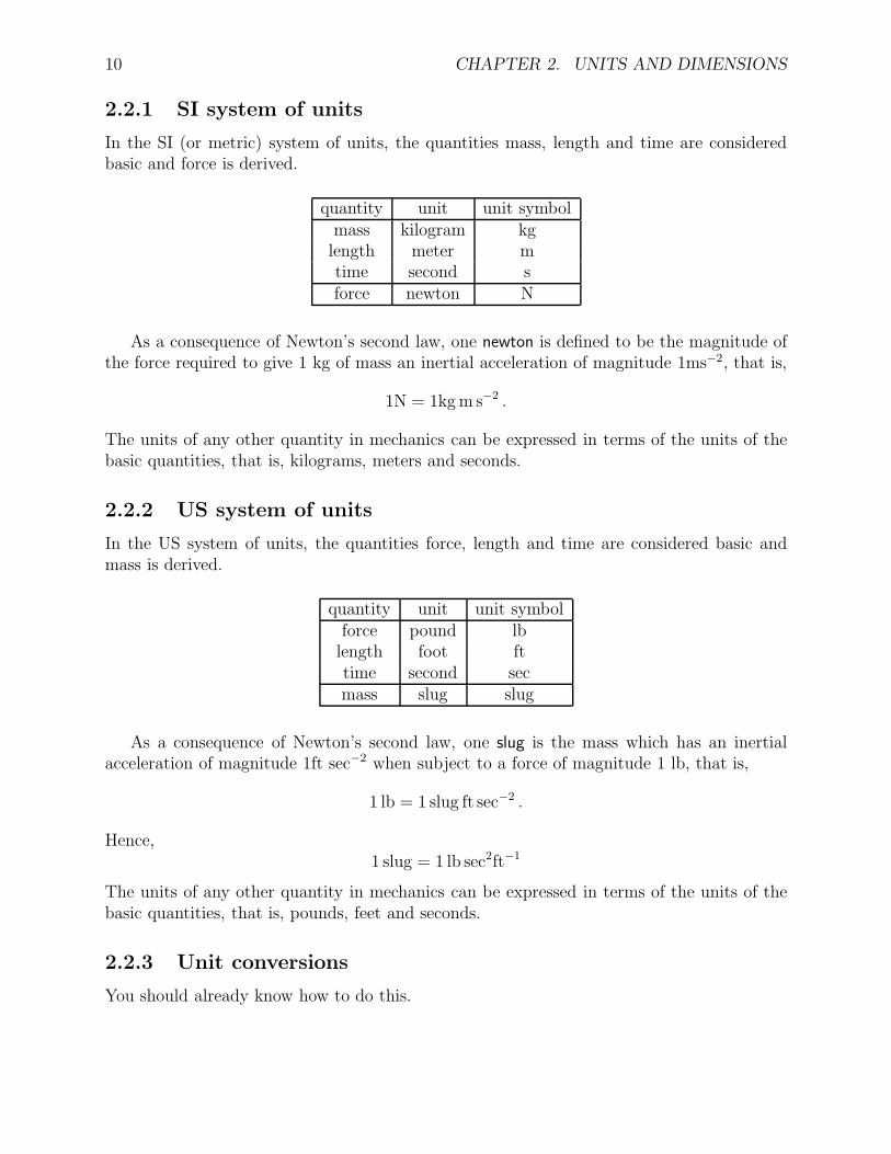
2.2.1 SI system of units
In the SI (or metric) system of units, the quantities mass, length and time are consideredbasic and force is derived.
quantity unit unit symbolmass kilogram kglength meter mtime second sforce newton N
As a consequence of Newton’s second law, one newton is defined to be the magnitude ofthe force required to give 1 kg of mass an inertial acceleration of magnitude 1ms−2, that is,
1N = 1kg m s−2 .
The units of any other quantity in mechanics can be expressed in terms of the units of thebasic quantities, that is, kilograms, meters and seconds.
2.2.2 US system of units
In the US system of units, the quantities force, length and time are considered basic andmass is derived.
quantity unit unit symbolforce pound lblength foot fttime second secmass slug slug
As a consequence of Newton’s second law, one slug is the mass which has an inertialacceleration of magnitude 1ft sec−2 when subject to a force of magnitude 1 lb, that is,
1 lb = 1 slug ft sec−2 .
Hence,1 slug = 1 lb sec2ft−1
The units of any other quantity in mechanics can be expressed in terms of the units of thebasic quantities, that is, pounds, feet and seconds.
2.2.3 Unit conversions
You should already know how to do this.

2.3. DIMENSIONS 11
2.3 Dimensions
To every quantity in mechanics, we associate a dimension. Dimension indicates quantitytype. We sometimes use symbols to indicate dimension. These symbols for the fundamentalquantities are given in the following table.
quantity dimension symbolforce Fmass Mlength Ltime T
Note that the concept of dimension is not the same as unit. One foot is not the same asone meter, however, both have the same dimension, namely, length.
2.3.1 Dimensional systems
The dimensions of the four fundamental quantities are related by Newton’s second law,specifically,
F = MLT−2.
Hence we can choose any three dimensions as basic dimensions and consider the fourth di-mension as a derived dimension. Usually, one chooses M, L, T or F, L, T as basic dimensions.
Absolute dimensional system. In the absolute dimensional system, mass, length andtime are considered basic and force is derived. The dimension of any quantity in mechanicsis expressed as
MαLβT γ
where α, β and γ are real numbers. For example, F = MLT−2.
Gravitational dimensional system. In the gravitational dimensional system, force,length and time are considered basic and mass is derived. The dimension of any quantity inmechanics is expressed as
F αLβT γ
where α, β and γ are real numbers. For example, M = FL−1T 2.

12 CHAPTER 2. UNITS AND DIMENSIONS
2.4 Dimensions of derived quantities
The dimension of any quantity Q in mechanics can be obtained using the following simplerules. We will use the notation dim[Q] to indicate the dimension of quantity Q. Thedimension of a vector quantity Q is considered to be the same as that of its magnitude, thatis, dim[Q] = dim[|Q|].
Dimensions of numbers. A “pure” number Q is considered dimensionless. We indicatethis by
dim[Q] = 1
Dimensions of products and quotients. If Q1 and Q2 are any two quantities, then
dim[Q1Q2] = dim[Q1] dim[Q2] and dim[Q1/Q2] = dim[Q1]/ dim[Q2] .
Example 1 (Angle) In radians, the angle θ is given by θ = S/R. Since S and R are
Figure 2.1: Angle
lengths, we have
dim[θ] = dim[S/R] = dim[S]/ dim[R] = L/L = 1 .
Since dim[θ] = 1, we consider angles dimensionless.
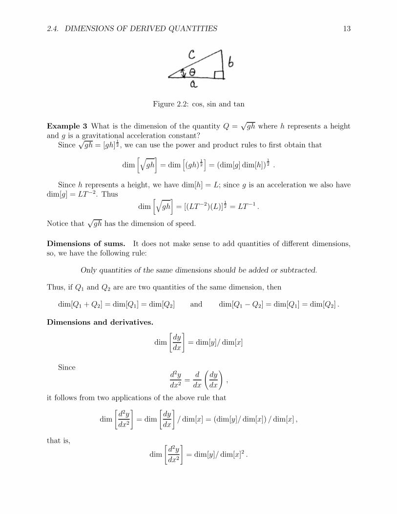
Example 2 (cos and sin ) Since cos θ = a/c, where a and c and lengths, we have
dim[cos θ] = dim[a/c] = dim[a]/ dim[c] = L/L = 1 .
In a similar fashion,
dim[sin θ] = dim[b/c] = dim[b]/ dim[c] = L/L = 1 .
and
dim[tan θ] = dim[b/a] = dim[b]/ dim[a] = L/L = 1 .
Dimensions of powers. If Q is any quantity and α is any real number, then
dim[Qα] = dim[Q]α .
2.4. DIMENSIONS OF DERIVED QUANTITIES 13
Figure 2.2: cos, sin and tan
Example 3 What is the dimension of the quantity Q =√
gh where h represents a heightand g is a gravitational acceleration constant?
Since√
gh = [gh]12 , we can use the power and product rules to first obtain that
dim[
√
gh]
= dim[
(gh)12
]
= (dim[g] dim[h])12 .
Since h represents a height, we have dim[h] = L; since g is an acceleration we also havedim[g] = LT−2. Thus
dim[
√
gh]
= [(LT−2)(L)]12 = LT−1 .
Notice that√
gh has the dimension of speed.
Dimensions of sums. It does not make sense to add quantities of different dimensions,so, we have the following rule:
Only quantities of the same dimensions should be added or subtracted.
Thus, if Q1 and Q2 are are two quantities of the same dimension, then
dim[Q1 + Q2] = dim[Q1] = dim[Q2] and dim[Q1 − Q2] = dim[Q1] = dim[Q2] .
Dimensions and derivatives.
dim
[
dy
dx
]
= dim[y]/ dim[x]
Sinced2y
dx2=
d
dx
(
dy
dx
)
,
it follows from two applications of the above rule that
dim
[
d2y
dx2
]
= dim
[
dy
dx
]
/ dim[x] = (dim[y]/ dim[x]) / dim[x] ,
that is,
dim
[
d2y
dx2
]
= dim[y]/ dim[x]2 .

14 CHAPTER 2. UNITS AND DIMENSIONS
Dimensions and integrals.
dim[∫
y dx]
= dim[y] dim[x]
Dimensions and equations. We say that an equation is dimensionally homogeneous ifevery term in the equation has the same dimension. We have the following rule:
All equations (in mechanics) must be dimensionally homogeneous.
Example 4 The expression for planar acceleration in polar coordinates is given by
a = (r + rθ2)er + (rθ + 2rθ)eθ
where er and eθ are dimensionless unit vectors. Let us check to see if every term in thisequation has the dimension of acceleration, that is, LT−2.
Example 5 Later we shall meet the inverse square gravitational law which is expressed as
F =GMm
r2
where F is a force magnitude, M and m are masses while r is a distance. Here we shalldetermine the dimension of G.

2.5. EXERCISES 15
2.5 Exercises
Exercise 1 Obtain expressions for the dimensions of the following quantities using (a) theabsolute dimensional system, and (b) the gravitational dimensional system. Here x and yare lengths, t is time, m is some mass, a is an acceleration and F represents a force.
(a) −√
10∫ x2
x1
a dx
(b)
√
√
√
√
(
dx
dt
)2
+
(
dy
dt
)2
(c)d2
dt2
(
∫ x(t)
0F (η) dη
)
Exercise 2 Determine whether or not the equation
d
dt
∫ x
0F dx =
1
2
dm
dtv2 + mva
is dimensionally homogeneous where F is a force, x is a displacement, v is a speed, a is anacceleration, m is some mass, and t is time.
Exercise 3 If m denotes a mass, g an acceleration magnitude, x a length, F a force mag-nitude and t time, determine whether or not the following equation is dimensional homoge-neous.
mgx =∫ x
0F dη + m
(
dx
dt
)2
+d2x
dt2
If not homogeneous, state why.
Exercise 4 You have just spent the whole evening deriving the following expression for anacceleration in an AAE 203 problem:
a = (lθ + dθΩ)s1 + dΩθs2
where l and d represent lengths, θ represents an angle, and Ω represents a rotation rate.Your roommate looks at the expression and without doing any kinematic calculations, saysyou are wrong. Could she/he be right? Justify your answer.
Exercise 5 Determine the dimension of h in order for the following equation to be dimen-sionally correct.
θ +h
lsin θ = 0
where θ represents an angle and l represents a length.

16 CHAPTER 2. UNITS AND DIMENSIONS
Exercise 6 Determine the dimension of k in order for the following equation to be dimen-sionally correct.
mx + kx = 0
where x represents a displacement and m represents a mass.
Exercise 7 Determine the dimension of ρ in order for the following equation to be dimen-sionally homogeneous.
mV = −1
2ρV 2CDS − W sin γ + T cos α
where W and T represent forces, m is a mass, V is a speed, α is an angle, S is an area andCD is dimensionless.
Exercise 8 Given that F is a force, x is a displacement, θ is an angle, and v is a speed,determine the dimensions of the quantities I and k in order that the following equation bedimensionally homogeneous.
∫ x
0F dx =
1
2I
(
dθ
dt
)2
+1
2kv2
Exercise 9 Determine whether or not the following equation is dimensionally homogeneous.
ml2θ + kx + mgsinθ = 0
where x and l represent lengths, θ represents an angle, m is a mass k is a spring constantand g is an acceleration.

Chapter 3
Vectors
3.1 Introduction
A scalar is a real number, for example, 1, −1/2,√
2. Some physical quantities can berepresented by a single scalar, for example, time, length, and mass. These quantities arecalled scalar quantities.
Other physical quantities cannot be represented by a single scalar, for example, forceand velocity. These quantities have attributes of magnitude and direction. In saying thata motorcycle is traveling south at a speed of 70 mph, we are specifying the velocity of thecycle in terms of magnitude (70 mph) and direction (south). To represent velocity, we needa mathematical concept which has the above two attributes. A vector is such a concept.Mathematically, we define a vector to be a directed line segment. Graphically, we usuallyindicate a vector by a line segment with an arrowhead, for example,
The magnitude of a vector is the length of the line segment while the direction of thevector is determined by the orientation of the line segment and the sense of the arrowhead.Sometimes a vector is indicated by a segment of a circle with an arrowhead; in this case thedirection of the vector is determined by the right-hand rule. In the figure below, the directionof each vector is perpendicular to and out of the page.
17

18 CHAPTER 3. VECTORS
All vectors, except unit vectors (we will meet these later), are represented by a symbolwith an overhead bar, for example, V , 0, ♣. If A and B are the endpoints of a vector V andthe direction of V is from A to B, we sometimes write V = AB.

3.1. INTRODUCTION 19
A
B
V
V = AB
If V = AB, we call A the tail or point of application of V and B is called the head of V .The line on which V lies is called the line of action of V .
V
A tail
B head
line of action
The magnitude or length of a vector V (denoted |V | and sometimes by V ) is the distancebetween the endpoints of V . Two vectors V and W are said to be parallel (denoted V // W ),if the lines of action of V and W are parallel.
Two vectors V , W , are defined to be equal, that is, W = V , if they have the same mag-nitude and direction. Thus one can completely specify a vector by specifying its magnitudeand direction.
V
W
W = V

20 CHAPTER 3. VECTORS
3.2 Vector addition
The sum or resultant of two vectors V and W is denoted by
V + W
We present two equivalent definitions of vector addition, the triangle law and the parallelogramrule.
Triangle law. Place the tail of W at the head of V . Then V + W is the vector from tailof V to the head of W .
V
W
W
V
V
W+
A B
C
In other words, if V = AB and W = BC, then V + W = AC.
Parallelogram rule. Place the tails of V and W together. Complete the parallelogramwith sides parallel to V and W . Then V + W lies along a diagonal of the parallelogram withtail at the tails of V and W .
V
W
W
V
VW+
A B
C
W
D
In other words, if V = AB and W = AC, then V +W = AD where ABDC is a parallelogram.
One may readily show that the above two definitions are equivalent.

3.2. VECTOR ADDITION 21
Some trigonometry Recall
anglesinecosine
Pythagorean theorem
c2 = a2 + b2
Cosine law:
c2 = a2 + b2 − 2ab cos θ
Sine Law
sin α
a=
sin β
b=
sin γ
c

22 CHAPTER 3. VECTORS
Example 6 (Vector addition, cosine law, sine law.)Given two vectors V and W as shown with |V | = 1 and |W | = 2. Find V + W .
Solution. We use the triangle law for vector addition as illustrated.
Using the cosine law on the above triangle, we obtain that
|V + W |2 = |V |2 + |W |2 − 2|V | |W | cos(120)
= (1)2 + (2)2 − 2(1)(2)(
−1
2
)
= 7 .
Hence,|V + W | =
√7 .
Applying the sine law to the above triangle yields
sin θ
|W | =sin(120)
|V + W | .
Hence,
sin θ =sin(120)|W ||V + W | =
(√
3/2)(2)√7
=
√
3
7
which yields
θ = sin−1
√
3
7
= 40.89 .

3.2. VECTOR ADDITION 23
So,
V + W is a vector of magnitude√
7 with direction as shown where θ = 40.89
(Recall that a vector can be completely specified by specifying its magnitude and direction.)
• A zero vector is a vector of zero magnitude.
· 0
• The negative of V (denoted −V ) is a vector which has the same magnitude as V butopposite direction.
VV
24 CHAPTER 3. VECTORS
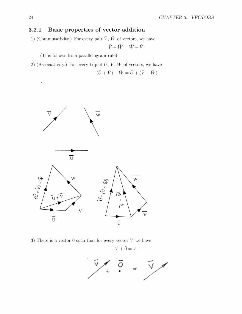
3.2.1 Basic properties of vector addition
1) (Commutativity.) For every pair V , W of vectors, we have
V + W = W + V .
(This follows from parallelogram rule)
2) (Associativity.) For every triplet U , V , W of vectors, we have
(U + V ) + W = U + (V + W )
.
V
U
W
UU
VV
W W
U + V
V+
W
U +
(V +
W)
(U +
V)
+ W
3) There is a vector 0 such that for every vector V we have
V + 0 = V .
3.2. VECTOR ADDITION 25
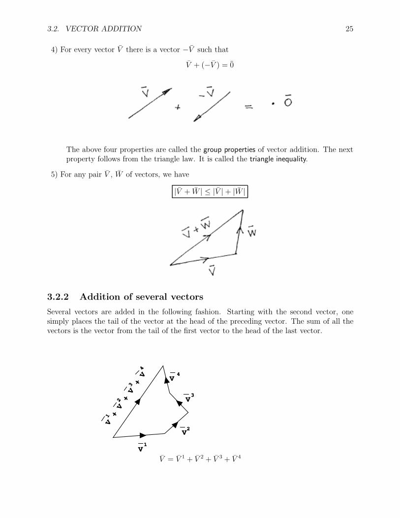
4) For every vector V there is a vector −V such that
V + (−V ) = 0
The above four properties are called the group properties of vector addition. The nextproperty follows from the triangle law. It is called the triangle inequality.
5) For any pair V , W of vectors, we have
|V + W | ≤ |V | + |W |
3.2.2 Addition of several vectors
Several vectors are added in the following fashion. Starting with the second vector, onesimply places the tail of the vector at the head of the preceding vector. The sum of all thevectors is the vector from the tail of the first vector to the head of the last vector.
V1 + V
2 + V
3 + V
4
1V
V2
V3
V4
V = V 1 + V 2 + V 3 + V 4

26 CHAPTER 3. VECTORS
3.2.3 Subtraction of vectors
The difference of two vectors V and W is denoted by V − W and is defined by
V − W = V + (−W ) .
V
W
V
W
V - W
Figure 3.1: Subtraction of vectors
Note that, if the tails of V are W are placed together then, V − W is the vector from thehead of V to the head of W .
3.3 Multiplication of a vector by a scalar
The product of a vector V and a scalar k is another vector and is denoted by
kV
The product kV is defined to be a vector whose magnitude is |k||V |. If k > 0, the directionof kV is the same as V ; if k < 0 the direction of kV is opposite to that of V . If k = 0, theproduct kV is zero.
VV2
V-2
Basic properties of scalar multiplication
1) k(V + W ) = kV + kW
2) (k + l)V = kV + lV
3) 1V = V
3.3. MULTIPLICATION OF A VECTOR BY A SCALAR 27
4) k(lV ) = (kl)V
The above four properties along with the group properties of vector addition are calledthe field properties of vectors.
The next property is actually part of the above definition of scalar multiplication.
5) |kV | = |k||V |
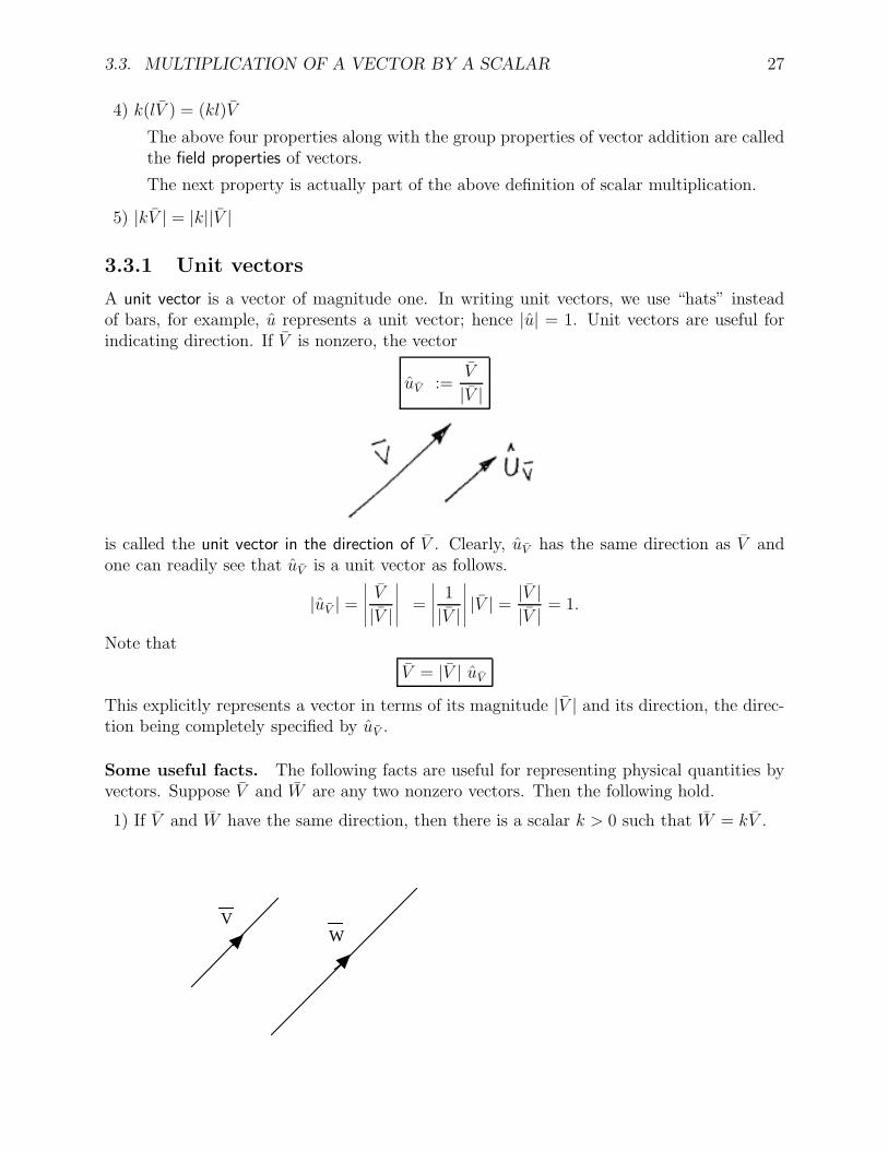
3.3.1 Unit vectors
A unit vector is a vector of magnitude one. In writing unit vectors, we use “hats” insteadof bars, for example, u represents a unit vector; hence |u| = 1. Unit vectors are useful forindicating direction. If V is nonzero, the vector
uV :=V
|V |
is called the unit vector in the direction of V . Clearly, uV has the same direction as V andone can readily see that uV is a unit vector as follows.
|uV | =
∣
∣
∣
∣
∣
V
|V |
∣
∣
∣
∣
∣
=
∣
∣
∣
∣
∣
1
|V |
∣
∣
∣
∣
∣
|V | =|V ||V | = 1.
Note that
V = |V | uV
This explicitly represents a vector in terms of its magnitude |V | and its direction, the direc-tion being completely specified by uV .
Some useful facts. The following facts are useful for representing physical quantities byvectors. Suppose V and W are any two nonzero vectors. Then the following hold.
1) If V and W have the same direction, then there is a scalar k > 0 such that W = kV .
VW

28 CHAPTER 3. VECTORS
2) If the direction of W is opposite to the direction of V , then there is a scalar k < 0 suchthat W = kV .
V
W
3) If W is parallel to V , then there is a nonzero scalar k such that W = kV .
We now demonstrate why the above facts are true.
1) Since W and V have the same direction, the unit vector in the direction of W is equalto the unit vector in the direction of V , that is,
W
|W | =V
|V | ;
hence,
W =|W ||V | V
or,
W = kV where k =|W ||V | > 0 .
2) In this case, −W has the same direction as V . Using the previous result, there is a scalarl > 0 such that
−W = lV .
Letting k := −l, we have
W = kV with k < 0 .
3) Since W is parallel to V , either W and V have the same direction or they have oppositedirection. Hence, using the previous two results,
W = kV where k < 0 or k > 0.

3.4. COMPONENTS 29
3.4 Components
So far, our concept of a vector is a geometrical one, specifically, it is a mathematical objectwith the properties of magnitude and direction. This representation is useful for initialrepresentation of physical quantities, for example, suppose one wants to describe the velocityof a motorcycle heading south at 70 mph as a vector. However, in manipulating vectors (forexample adding them) the geometric representation can become very cumbersome if notimpossible. In this section, we learn how to represent any vector as an ordered triplet ofscalars, for example (1, 2, 3). This permits us to reduce operations on vectors to operationson scalars.
3.4.1 Planar case
Consider first the case in which all vectors of interest lie in a single plane,
Fact 1 Suppose b1, b2, are any pair of non-zero, non-parallel vectors in a plane. Then, forevery vector V in the plane, there is a unique pair of scalars, V1, V2 such that
V = V1 b1 + V2 b2
The pair (b1, b2) of vectors is called a basis. It defines a coordinate system. With respectto this basis, V1b1 and V2b2 are called the vector components of V ; the scalars V1 and V2 arecalled the scalar components or coordinates of V . The important thing about a basis is thatit permits one to represent uniquely any vector V in the plane as a pair of scalars (V1, V2).
V
b 1
b 2
Demonstration of Fact 1. Construct a parallelogram with V as diagonal and with sidesparallel to b1 and b2. Let V1 and V2 be the vectors with tails at the tail of V which make uptwo sides of the parallelogram as shown. Then V1 is parallel to b1, V2 is parallel to b2 andfrom the parallelogram law
V = V1 + V2
Also, since V1 is parallel to b1 and V2 is parallel to b2, there are unique scalars V1, V2 so that
V1 = V1b1 and V2 = V2b2 .
Thus, V may be written as V = V1b1 + V2b2.

30 CHAPTER 3. VECTORS
b2
2V
V
1V
b1
Example 7 (Planar components.) Given the coplanar vectors V , b1, b2 as shown where|V | = 5, find
(i) scalars V1 and V2 such that V = V1b1 + V2b2,
(ii) scalars n1 and n2 such that uV = n1b1 + n2b2.
Solution.
(i)
From the above parallelogram, it should be clear that
V = V1 + V2 .

3.4. COMPONENTS 31
Also, θ = 180 − 60 − 45 = 75. Using the sine law, we obtain that
sin θ
|V1|=
sin 45
|V | .
Hence,
|V1| =sin(75)|V |
sin 45=
(0.9659)(5)1√2
= 6.830 .
So, V1 = |V1| b1 = 6.830 b1. Using the sine law again,
sin 60
|V2|=
sin 45
|V | .
Hence,
|V2| =sin 60
sin 45|V | =
(√3
2
)
(5)1√2
=5√
3√2
= 6.124 .
So, V2 = |V2| b2 = 6.124 b2 and
V = 6.830 b1 + 6.124 b2
Note that, in this example, |V1|, |V2| > |V | .
(ii) Since,
uV =V
|V | =1
5(6.830 b1 + 6.124 b2)
we obtain that
uV = 1.366 b1 + 1.225 b2
Perpendicular components
Consider the special case in which b1 = e1, b2 = e2 and e1, e2 are mutually perpendicularunit vectors.
V1
1
2e 1e
Then, the parallelogram used in obtaining components V1 and V2 is a rectangle and thecomponents are sometimes called rectangular components.
32 CHAPTER 3. VECTORS
e2
e1
P
AO
V2
V1
V
θ
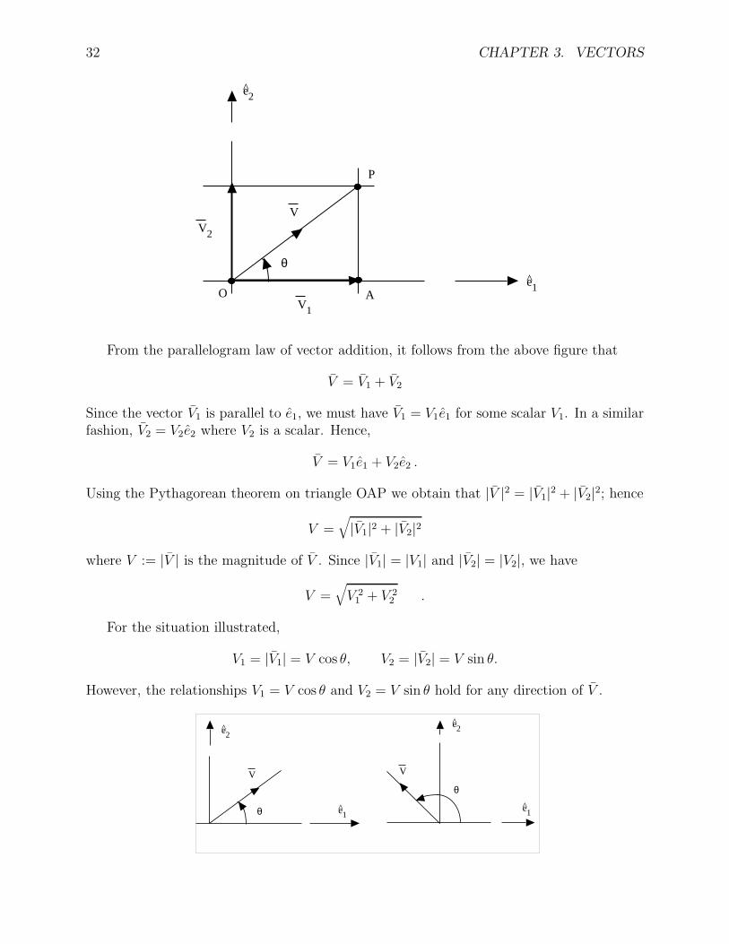
From the parallelogram law of vector addition, it follows from the above figure that
V = V1 + V2
Since the vector V1 is parallel to e1, we must have V1 = V1e1 for some scalar V1. In a similarfashion, V2 = V2e2 where V2 is a scalar. Hence,
V = V1e1 + V2e2 .
Using the Pythagorean theorem on triangle OAP we obtain that |V |2 = |V1|2 + |V2|2; hence
V =√
|V1|2 + |V2|2
where V := |V | is the magnitude of V . Since |V1| = |V1| and |V2| = |V2|, we have
V =√
V 21 + V 2
2 .
For the situation illustrated,
V1 = |V1| = V cos θ, V2 = |V2| = V sin θ.
However, the relationships V1 = V cos θ and V2 = V sin θ hold for any direction of V .
e2
e1
V
θ
θ
V
e2
e1

3.4. COMPONENTS 33
Summarizing, we have the following relationships:
V = V1e1 + V2e2
V1 = V cos θ, V2 = V sin θ
Also,
V =√
V 21 + V 2
2
tan θ = V2/V1
3.4.2 General case
Suppose b1, b2 and b3 are any three non-zero vectors which are not parallel to a commonplane. Then, given any vector V , there exists a unique triplet of scalars, V1, V2, V3 such that
V = V1b1 + V2b2 + V3b3 .
The triplet of vectors, (b1, b2, b3), is called a basis. It defines a coordinate system. Withrespect to this basis, the vectors V1b1, V2b2, V3b3 are the vector components of V and thescalars V1, V2, V3 are the scalar components or coordinates of V . The most important thingabout a basis is that it permits one to represent uniquely any vector V as a triplet of scalars(V1, V2, V3). In this course, we consider mainly a special case, namely the case in whichb1, b2, b3 are mutually perpendicular unit vectors.
Mutually perpendicular components
Let e1, e2, e3 be any three mutually orthogonal (perpendicular) unit vectors. We call (e1, e2, e3)an orthogonal triad. Since (e1, e2, e3) constitute a basis, any vector V can be uniquely resolved
Figure 3.2: An orthogonal triad
into components parallel to e1, e2, e3, that is, there are unique scalars V1, V2, V3 such that
V = V1e1 + V2e2 + V3e3
The vectors V1e1, V2e2, V3e3 are called rectangular components and the scalars V1, V2, V3 arecalled rectangular scalar components or rectangular coordinates. Also,
34 CHAPTER 3. VECTORS
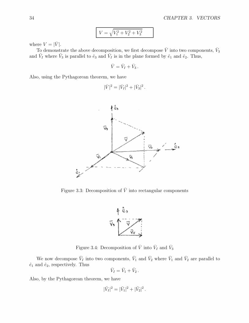
V =√
V 21 + V 2
2 + V 23
where V = |V |.To demonstrate the above decomposition, we first decompose V into two components, V3
and VI where V3 is parallel to e3 and VI is in the plane formed by e1 and e2. Thus,
V = VI + V3 .
Also, using the Pythagorean theorem, we have
|V |2 = |VI |2 + |V3|2 .
Figure 3.3: Decomposition of V into rectangular components
Figure 3.4: Decomposition of V into VI and V3
We now decompose VI into two components, V1 and V2 where V1 and V2 are parallel toe1 and e2, respectively. Thus
VI = V1 + V2 .
Also, by the Pythagorean theorem, we have
|VI |2 = |V1|2 + |V2|2 .

3.4. COMPONENTS 35
Figure 3.5: Decomposition of V into VI and V3
By combining the above two decompositions, we obtain that
V = V1 + V2 + V3
and|V |2 = |V1|2 + |V2|2 + |V3|2 .
Since V1 = V1e1, V2 = V2e2 and V3 = V3e3 with |V1|2 = V 21 , |V2|2 = V 2
2 and |V3|2 = V 23 , we
obtain the desired result, namely,
V = V1e1 + V2e2 + V3e3 and |V | = (V 21 + V 2
2 + V 23 )1/2 .
With the above decomposition, we can regard the vector V as the diagonal of a rectan-gular box with edges parallel to e1, e2, e3 and with dimensions |V1|, |V2| and |V3|.
Figure 3.6: V in a box

36 CHAPTER 3. VECTORS
Example 8 Given V and the orthogonal triad (u1, u2, u3) as shown, find
(i) scalars V1, V2, V3, such that V = V1u1 + V2u2 + V3u3
(ii) scalars n1, n2, n3, such that uV = n1u1 + n2u2 + n3u3 .
Solution:
(i) Clearly,
V = V1 + V2 + V3
where V1, V2, V3 are as shown.

3.4. COMPONENTS 37
Also,
V1 = |V1|u1 = 1u1 = u1
V2 = |V2|u2 = 2u2
V3 = |V3|u3 = 3u3
Thus,V = u1 + 2u2 + 3u3 ,
or, V = V1u1 + V2u2 + V3u3 where
V1 = 1, V2 = 2, V3 = 3
(ii) Since
|V | =√
V 21 + V 2
2 + V 23 =
√
(1)2 + (2)2 + (3)2 =√
14 ,
we have
uV =V
|V | =1√14
(u1 + 2u2 + 3u3) =1√14
u1 +2√14
u2 +3√14
u3
= 0.2673 u1 + 0.5345 u2 + 0.8018 u3
So, uV = n1u1 + n2u2 + n3u3 where
n1 = 0.2673, n2 = 0.5345, n3 = 0.818
Example 9 Given the vector V and the orthogonal triad (u1, u2, u3) as shown where
α = 63.43 , β = 53.30 , |V | = 3.742 ,
find scalars V1, V2, V3 such that V = V1u1 + V2u2 + V3u3.

38 CHAPTER 3. VECTORS
Solution:
Clearly,V = VI + V3
with|VI | = |V | cos β = 3.742 cos(53.3) = 2.236
and|V3| = |V | sin β = 3.742 sin(53.3) = 3.000 .
Also,V3 = |V3|u3 = 3u3
Considering the decomposition of VI , we have
VI = V1 + V2
with
|V1| = |VI | cosα = 2.236 cos(63.43) = 1.000
V1 = |V1|u1 = u1
and
|V2| = |VI | sinα = 2.236 sin(63.43) = 2.000
V2 = |V2|u2 = 2u2
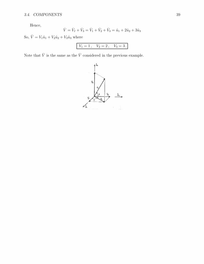
3.4. COMPONENTS 39
Hence,V = VI + V3 = V1 + V2 + V3 = u1 + 2u2 + 3u3
So, V = V1u1 + V2u2 + V3u3 where
V1 = 1 , V2 = 2 , V3 = 3 .
Note that V is the same as the V considered in the previous example.
40 CHAPTER 3. VECTORS
Example 10
Example 11

3.4. COMPONENTS 41
Addition of vectors via addition of scalar components
IfV = V1e1 + V2e2 + V3e3 and W = W1e1 + W2e2 + W3e3
then, using the field properties of vectors, one readily obtains that
V + W = (V1 +W1)e1 +(V2 +W2)e2 +(V3 +W3)e3
Scalar multiplication of a vector via multiplication of its scalar components
IfV = V1e1 + V2e2 + V3e3
then, using the field properties of vectors, one readily obtains that
kV = (kV1)e1 + (kV2)e2 + (kV3)e3
42 CHAPTER 3. VECTORS
3.5 Products of Vectors
Before discussing products of vectors, we need to examine what we mean by the anglebetween two vectors.
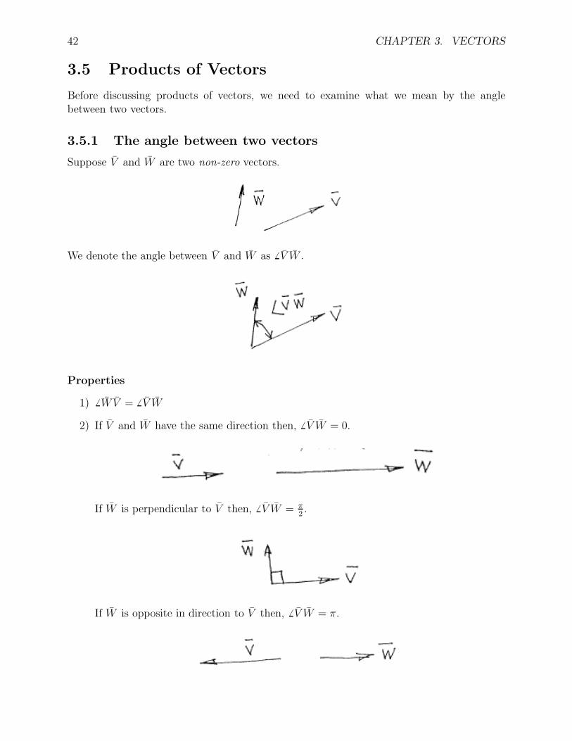
3.5.1 The angle between two vectors
Suppose V and W are two non-zero vectors.
We denote the angle between V and W as 6 V W .
Properties
1) 6 W V = 6 V W
2) If V and W have the same direction then, 6 V W = 0.
If W is perpendicular to V then, 6 V W = π2.
If W is opposite in direction to V then, 6 V W = π.

3.5. PRODUCTS OF VECTORS 43
3) In general, 0 ≤ 6 V W ≤ π.
0 < 6 V W <π
2
π
2< 6 V W < π
3.5.2 The scalar (dot) product of two vectors
Suppose V and W are any two non-zero vectors.
The scalar (or dot) product of V and W is a scalar which is denoted by V · W and isdefined by
V · W = V W cos θ
where V is the magnitude of V , W is the magnitude of W , and θ is the angle between V andW .
If either V or W is the zero vector, then, V · W is defined to be zero which also equalsV W cos θ for any value of θ.
Remarks
1) Since −1 ≤ cos θ ≤ 1, we have
−V W ≤ V · W ≤ V W

44 CHAPTER 3. VECTORS
2) Suppose V 6= 0 and W 6= 0. Then
θ = 0 ⇐⇒ V · W = V W
0 ≤ θ <π
2⇐⇒ V · W > 0
θ =π
2⇐⇒ V · W = 0
π
2< θ ≤ π ⇐⇒ V · W < 0
θ = π ⇐⇒ V · W = −V W
3) Since the angle between V and itself is zero, it follows that V · V = V 2; hence themagnitude of V can be expressed as
V = (V · V )1/2 .
4) If V and W represent physical quantities,
dim[V · W ] = dim[V ] dim[W ]
Basic Properties of the scalar product
1) V · W = W · V (commutativity)
2) U · (V + W ) = U · V + U · W
3) V · (kW ) = k(V · W )

3.5. PRODUCTS OF VECTORS 45
The scalar product and rectangular components
Suppose (e1, e2, e3) is any orthogonal triad.
Facts
(1)
ei · ej =
1 i = j0 i 6= j
= δij
For example,
e1 · e1 = |e1|2 = 1
e1 · e2 = |e1| |e2| cos(
π
2
)
= 0
(2) If V = V1e1 + V2e2 + V3e3, then
V1 = V · e1 , V2 = V · e2 , V3 = V · e3
Proof. Consider V1. Using the properties of the dot product, we obtain that
V · e1 = (V1e1 + V2e2 + V3e3) · e1
= V1(e1 · e1) + V2(e2 · e1) + V3(e3 · e1)
= V1(1) + V2(0) + V3(0) = V1 .
Similarly for V2 and V3.
(3) If
V = V1e1 + V2e2 + V3e3 and W = W1e1 + W2e2 + W3e3 ,
then
V · W = V1W1 + V2W2 + V3W3

46 CHAPTER 3. VECTORS
Proof. Using the properties of the dot product and the previous result, we obtain that
V · W = V · (W1e1 + W2e2 + W3e3)
= W1(V · e1) + W2(V · e2) + W3(V · e3)
= W1V1 + W2V2 + W3V3 .
(4) If θ is the angle between V and W then,
cos θ =V1W1 + V2W2 + V3W3
V W
where V = |V | and W = |W |.Proof. Recall that
V W cos θ = V · W = V1W1 + V2W2 + V3W3 .
Hence,
cos θ =V1W1 + V2W2 + V3W3
V W.
Also note that
θ = cos−1(
V1W1 + V2W2 + V3W3
V W
)
Example 12 Suppose
V = e1 + e2 + e3 and W = e1 − e3 .
ThenV · W = (1)(1) + (1)(0) + (1)(−1) = 0.
Since V · W is zero, V is perpendicular to W .
Example 13 Suppose
V = e1 + e2 + e3 and W = e1 + e3 .
Then
V · W = (1)(1) + (1)(0) + (1)(1) = 2 (3.1)
V = (1)2 + (1)2 + (1)2 = 3 (3.2)
W = (1)2 + (0)2 + (1)2 = 2 (3.3)
and
cos θ =V · WV W
= 1/3
Henceθ = cos−1(1/3) = 1.230 rad = 70.53

3.5. PRODUCTS OF VECTORS 47
3.5.3 Cross (vector) product of two vectors
Suppose V and W are any two non-zero non-parallel vectors.
The cross (or vector) product of V and W is a vector which is denoted by V × W and isdefined by
V × W = V W sin θ n
where V is the magnitude of V , W is the magnitude of W , θ is the angle between V andW and n is the unit vector which is normal (perpendicular) to both V and W and whosedirection is given by the right-hand rule.
Figure 3.7: Cross product
If V and W are parallel or either of them equals 0 then, V × W is defined to be the zerovector.
Remarks
(1) Since 0 ≤ sin θ ≤ 1 for 0 ≤ θ ≤ π, it follows that
|V × W | = V W sin θ
and|V × W | ≤ V W .
(2) Suppose V and W are both nonzero. Then the following relationships hold.
V × W = 0 ⇐⇒ V is parallel to W
|V × W | = V W ⇐⇒ V is perpendicular to W
(3) If V and W represent physical quantities, then
dim [V × W ] = dim[V ] dim[W ] .

48 CHAPTER 3. VECTORS
Figure 3.8: Sine function
Basic Properties of the cross product.
1) W × V = −V × W (not commutative)
2) U × (V + W ) = (U × V ) + (U × W ) and (U + V ) × W = (U × V ) + (U × W )
3) V × (kW ) = (kV ) × W = k(V × W )
Cross product and rectangular components
An orthogonal triad, (e1, e2, e3), is said to be right-handed if
e3 = e1 × e2
From now on, we shall consider only right-handed orthogonal triads.

3.5. PRODUCTS OF VECTORS 49
ˆ e 3
ˆ e 2
ˆ e 1
ˆ e 3 = ˆ e 1 × ˆ e 2
ˆ e 2
ˆ e 1ˆ e 3
Facts(1)
e1 × e1 = 0 e1 × e2 = e3 e1 × e3 = −e2
e2 × e1 = −e3 e2 × e2 = 0 e2 × e3 = e1
e3 × e1 = e2 e3 × e2 = −e1 e3 × e3 = 0
These relationships are illustrated below.
ˆ e 1 ˆ e 2 ˆ e 3 ˆ e 1 ˆ e 2
(2) IfV = V1e1 + V2e2 + V3e3 and W = W1e1 + W2e2 + W3e3 ,
thenV × W = (V2W3 − V3W2) e1 + (V3W1 − V1W3) e2 + (V1W2 − V2W1) e3
Proof. Exercise
(3) the above expression for V × W may also be obtained from
V × W = det
e1 e2 e3
V1 V2 V3
W2 W2 W3
where det denotes determinant.Proof. Exercise

50 CHAPTER 3. VECTORS
3.5.4 Triple products
Scalar triple product
The scalar triple product of three vectors U , V and W is the scalar defined by
U · (V × W )
Facts
(1)
U · (V × W ) = det
U1 U2 U3
V1 V2 V3
W1 W2 W3
(2)
U · (V × W ) = (U × V ) · W
that is, · and × can be interchanged.Proof. Exercise
Vector triple product
The vector triple product of three vectors U , V and W is the vector defined by
U × (V × W )
Facts
(1) In general,U × (V × W ) 6= (U × V ) × W .
For example,
e1 × (e1 × e2) = e1 × e3 = −e2
(e1 × e1) × e2 = 0 × e2 = 0
(2)
U ×(V ×W ) = (U ·W )V −(U · V )W
Proof. Exercise

Chapter 4
Kinematics of Points
In kinematics, we are concerned with motion without being concerned about what causesthe motion. If a body is small in comparison to its “surroundings”, we can view the bodyas occupying a single point at each instant of time. We will also be interested in the motionof points on “large” bodies. The kinematics of points involves the concepts of time, position,velocity and acceleration.
4.1 Derivatives
To involve ourselves with kinematics, we need derivatives.
4.1.1 Scalar functions
First, consider the situation where v is a scalar function of a scalar variable t. Suppose t1 isa specific value of t. Then the formal definition of the derivative of v at t1 is
dv
dt(t1) = lim
t→t1
v(t) − v(t1)
t − t1
Sometimes this is called the first derivative of v. Oftentimes, dvdt
is denoted by v. A graphicalrepresentation is given in Figure 4.1.
Figure 4.1: Derivative of a scalar function
The second derivative of v, denoted by d2vdt2
or v, is defined as the derivative of the firstderivative of v, that is
d2v
dt2=
d
dt
(
dv
dt
)
.
51
52 CHAPTER 4. KINEMATICS OF POINTS
In evaluating derivatives, we normally do not have to resort to the above definition. Byknowing the derivatives of commonly used functions (such as cos, sin, and polynomials) andusing the following properties, one can usually compute the derivatives of most commonlyencountered functions.
Properties. The following hold for any two scalar functions v and w.
(a)
d
dt(v + w) =
dv
dt+
dw
dt
(b) (Product rule)d
dt(vw) =
dv
dtw + v
dw
dt
(c) (Quotient rule) Whenever w(t) 6= 0,
d
dt
(
v
w
)
=dvdt
w − v dwdt
w2
(d) (Chain rule)d
dt(v(w)) =
dv
dw
dw
dt
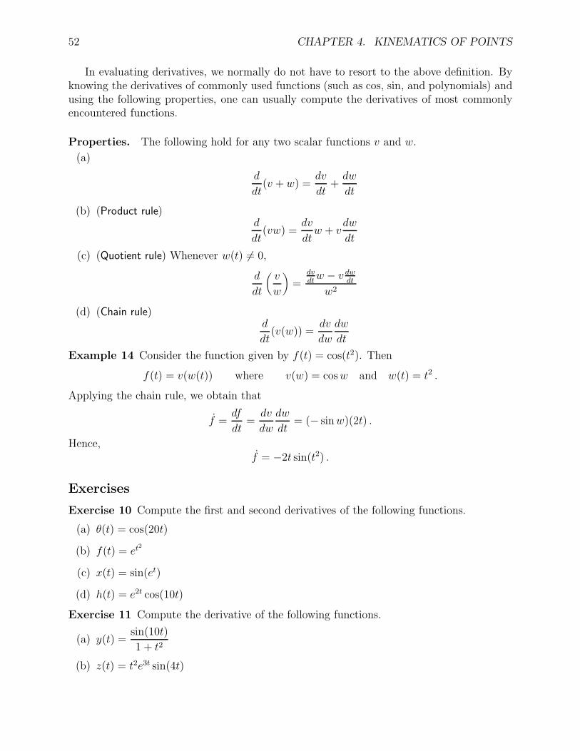
Example 14 Consider the function given by f(t) = cos(t2). Then
f(t) = v(w(t)) where v(w) = cos w and w(t) = t2 .
Applying the chain rule, we obtain that
f =df
dt=
dv
dw
dw
dt= (− sin w)(2t) .
Hence,f = −2t sin(t2) .
Exercises
Exercise 10 Compute the first and second derivatives of the following functions.
(a) θ(t) = cos(20t)
(b) f(t) = et2
(c) x(t) = sin(et)
(d) h(t) = e2t cos(10t)
Exercise 11 Compute the derivative of the following functions.
(a) y(t) =sin(10t)
1 + t2
(b) z(t) = t2e3t sin(4t)

4.1. DERIVATIVES 53
4.1.2 Vector functions
Consider now the situation where V is a vector function of a scalar variable t. Suppose t1 isa specific value of t. Then the formal definition of the derivative of V at t1 is
dV
dt(t1) = lim
t→t1
V (t) − V (t1)
t − t1
Oftentimes, dVdt
is denoted by ˙V .
Properties. The following hold for any two vector functions V and W and any scalarfunction k.
(a)
d
dt(V + W ) =
dV
dt+
dW
dt
(b)
d
dt(kV ) =
dk
dtV + k
dV
dt
(c)
d
dt(V · W ) =
dV
dt· W + V · dW
dt
(d)
d
dt(V × W ) =
dV
dt× W + V × dW
dt
(e) (Chain rule)d
dt(V (k)) =
dk
dt
dV
dk
Derivatives and components. Usually we evaluate the derivative of a vector functionby differentiating its scalar components. Suppose e1, e2, e3 is a set of constant basis vectorsand
V (t) = V1(t)e1 + V2(t)e2 + V3(t)e3 .
Then, using properties (a) and (b) above, we obtain that
dV
dt=
dV1
dte1 +
dV2
dte2 +
dV3
dte3
or˙V = V1e1 + V2e2 + V3e3

54 CHAPTER 4. KINEMATICS OF POINTS
4.1.3 The frame derivative of a vector function
We define a reference frame (or frame of reference) to be an right-handed orthogonal triad ofunit vectors which have the same point of application. Figure 4.2 illustrates several referenceframes. Usually we use a single symbol to reference frame; thus the reference frame consisting
Figure 4.2: Reference frames
of the vectors f1, f2, f3 will be referred to as the reference frame f .Consider a time-varying vector V . If one observes this vector from different reference
frames then, one will observe different variations of V with time. For that reason, we havethe following definition.
Figure 4.3: The frame derivative of a vector
The derivative of V in f is denoted byfdVdt
and is defined by
fdV
dt=
dV1
dtf1 +
dV2
dtf2 +
dV3
dtf3
where V1, V2, V3 are the scalar components of V relative to f , that is,
V = V1f1 + V2f2 + V3f3 .
Oftentimes,fdVdt
is denoted by f V . Thus,
f ˙V = V1f1 + V2f2 + V3f3

4.1. DERIVATIVES 55
Properties. The following hold for any two vector functions V and W and any scalarfunction k.
(a)
fd
dt(V + W ) =
fdV
dt+
fdW
dt
(b)
fd
dt(kV ) =
dk
dtV + k
fdV
dt
(c)
fd
dt(V · W ) =
fdV
dt· W + V ·
fdW
dt
(d)
fd
dt(V × W ) =
fdV
dt× W + V ×
fdW
dt
(e) (Chain rule)fd
dt(V (k)) =
dk
dt
fdV
dk

56 CHAPTER 4. KINEMATICS OF POINTS
Example 15 (Frame derivative)

4.1. DERIVATIVES 57
Exercises
Exercise 12 Consider the reference frames f = (f1, f2, f3) and g = (g1, g2, g3) as illustratedwhere θ = 2t rads. Suppose the vector Z is given by
Z = 2tg1 + t2g2 .
In terms of t and the units vectors of g, find expressions for the following quantities.
(a) g ˙Z
(b) f ˙Z
(c) gZ + ω × Z where ω = θg3
Compare the answers for parts (b) and (c).

58 CHAPTER 4. KINEMATICS OF POINTS
4.2 Basic definitions
Besides time, there are three additional basic concepts in the kinematics of points, namely,position, velocity, and acceleration.
4.2.1 Position
Consider any two points O and P . We define the position of P relative to O (denoted rOP )or the position vector from O to P as the vector from O to P , that is,
rOP := OP
Figure 4.4: Position vector, rOP
Clearly, the position of a point O relative to itself is the zero vector, that is,
rOO = 0 .
It should also be clear that the position of O relative to P is the negative of the positionof P relative to O, that is,
rPO = −rOP .
Figure 4.5: rPO
Composition of position vectors. For any three points O, P, Q, we have
rOQ = rOP + rPQ (4.1)
This follows from the triangle law of vector addition and is illustrated in Figure 4.6.From the above relationship, we also have
rPQ = rOQ − rOP .

4.2. BASIC DEFINITIONS 59
Figure 4.6: Composition of position vectors
Consider now several points, P1, P2, . . . , Pn. Then, by repeated application of result (4.1),we obtain
rP1Pn = rP1P2 + rP2P3 + . . . + rPn−1Pn .
This is illustrated in Figure 4.7.
Figure 4.7: Composition of several position vectors
4.2.2 Velocity and acceleration
Suppose we are observing the motion of some point P from a reference frame f . We firstdemonstrate the following result.
If O and O′ are any two points which are fixed in reference frame f , then
fd
dtrOP =
fd
dtrO′P
To see this, first note thatrOP = rOO′
+ rO′P .
Hence,fd
dtrOP =
fd
dtrOO′
+fd
dtrO′P
Since points O and O′ are fixed in f , the vector rOO′
is a fixed vector in f , hence
fd
dtrOO′
= 0

60 CHAPTER 4. KINEMATICS OF POINTS
Figure 4.8: Independence of velocity on origin
and the desired result follows.
We define the velocity of P in f (denoted fvP ) by
fvP :=fd
dtrOP
where O is any point fixed in f . The speed of P in f is | fvP |, the magnitude of the velocityof P in f .
Figure 4.9: The velocity of P in f
We define the acceleration of P in f (denoted faP ) by
faP :=fd
dtfvP

4.2. BASIC DEFINITIONS 61
Note thatfaP =
fd2
dt2rOP
In the next section, we consider some special types of motions. First we have someexamples to illustrate the above concepts.
Example 16 (Pendulum with moving support)

62 CHAPTER 4. KINEMATICS OF POINTS
Example 17 (Bug on bar on cart)

4.2. BASIC DEFINITIONS 63
Exercises
Exercise 13 The two link planar manipulator is constrained to move in the plane definedby the vectors e1 and e2 of reference frame e. Point O is fixed in e.
Find expressions for evP and eaP in terms of θ1, θ2, their first and second time derivatives,l1, l2 and e1, e2, e3.
Exercise 14 The small ball P moves in the straight slot which is fixed in the disk. Relativeto reference frame e, point O is fixed and the disk rotates about an axis through O which isparallel to e3 and perpendicular to the plane of the disk.

64 CHAPTER 4. KINEMATICS OF POINTS
Find expressions for evP and eaP in terms of l, r, θ, r, θ, r, θ and unit vectors fixed inthe disk.
4.3. RECTILINEAR MOTION 65
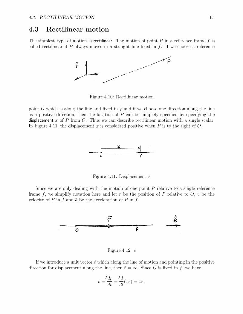
4.3 Rectilinear motion
The simplest type of motion is rectilinear. The motion of point P in a reference frame f iscalled rectilinear if P always moves in a straight line fixed in f . If we choose a reference
Figure 4.10: Rectilinear motion
point O which is along the line and fixed in f and if we choose one direction along the lineas a positive direction, then the location of P can be uniquely specified by specifying thedisplacement x of P from O. Thus we can describe rectilinear motion with a single scalar.In Figure 4.11, the displacement x is considered positive when P is to the right of O.
Figure 4.11: Displacement x
Since we are only dealing with the motion of one point P relative to a single referenceframe f , we simplify notation here and let r be the position of P relative to O, v be thevelocity of P in f and a be the acceleration of P in f .
Figure 4.12: e
If we introduce a unit vector e which along the line of motion and pointing in the positivedirection for displacement along the line, then r = xe. Since O is fixed in f , we have
v =fdr
dt=
fd
dt(xe) = xe .

66 CHAPTER 4. KINEMATICS OF POINTS
The last equality above follows from the fact that e is a constant vector in reference framef . We also have that
a =fdv
dt=
fd
dt(xe) = xe .
So, summarizing, we have
r = xe , v = ve , a = ae
where
v = x and a = v = x . (4.2)
4.4 Planar motion
The motion of point P in a reference frame f is called planar if P always moves in a planewhich is fixed in f .
Figure 4.13: Planar motion
If we choose a reference point O which is in the plane and fixed in f , then the locationof P can be uniquely specified by specifying the position of P relative to O. For the rest ofthis section, we let r be the position of P relative to O, v be the velocity of P in f and a bethe acceleration of P in f . Hence
v =dr
dtand a =
dv
dt
where it is understood that the above differentiations are carried out relative to frame f .In general, planar motion can be described with two scalar coordinates. We now consider
two different coordinate systems for describing planar motion, namely cartesian coordinatesand polar coordinates.
4.4.1 Cartesian coordinates
Choose any two mutually perpendicular lines in the plane passing through O and fixed inf . By choosing a positive direction for each line, The location of point P can be uniquelydetermined by the cartesian coordinates x and y as illustrated in Figure 4.14.
We now compute expressions for r, v and a in terms of cartesian coordinates. To thisend, we introduce unit vectors e1, e2 fixed in the plane as illustrated in Figure 4.15. Then,
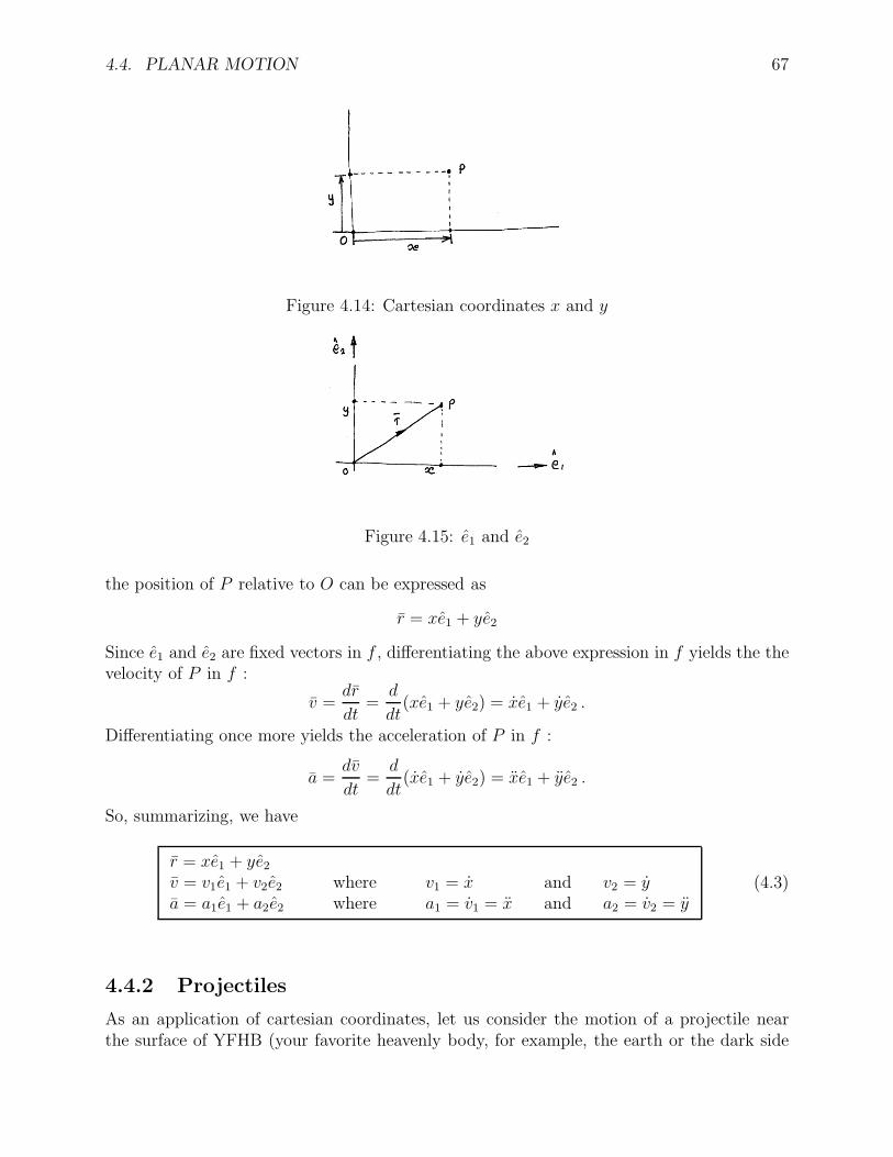
4.4. PLANAR MOTION 67
Figure 4.14: Cartesian coordinates x and y
Figure 4.15: e1 and e2
the position of P relative to O can be expressed as
r = xe1 + ye2
Since e1 and e2 are fixed vectors in f , differentiating the above expression in f yields the thevelocity of P in f :
v =dr
dt=
d
dt(xe1 + ye2) = xe1 + ye2 .
Differentiating once more yields the acceleration of P in f :
a =dv
dt=
d
dt(xe1 + ye2) = xe1 + ye2 .
So, summarizing, we have
r = xe1 + ye2
v = v1e1 + v2e2 where v1 = x and v2 = ya = a1e1 + a2e2 where a1 = v1 = x and a2 = v2 = y
(4.3)
4.4.2 Projectiles
As an application of cartesian coordinates, let us consider the motion of a projectile nearthe surface of YFHB (your favorite heavenly body, for example, the earth or the dark side

68 CHAPTER 4. KINEMATICS OF POINTS
Figure 4.16: Projectile motion
of the moon). Suppose that a projectile P is launched from point O on YFHB at a launchangle θ and with launch speed v relative to YFHB. Modeling YFHB as flat and neglectingall forces other than gravitational forces, then relative to YFHB, P move in a vertical planeand its acceleration is given by
a = gg
where g is the unit vector in the direction of the local vertical and g is the gravitationalacceleration of YFHB. We will show this fact later in the course.
Introduce reference frame e fixed in YFHB with origin at O as shown. Then, the positionof P is completely described by the cartesian coordinates x, y where y is the height of Pabove the surface of YFHB and we call x the horizontal range. Let v and a be the velocityand acceleration, respectively, of P in e. Then,
a = −ge2 .
Hence, it follows from (4.3) that
x = 0 and y = −g . (4.4)
Choosing t to be zero when P is launched from O, the velocity of P at launch, that is v(0),is given by
v(0) = v cos θ e1 + v sin θ e2 .
Hence, it follows from (4.3) that
x(0) = v cos θ and y(0) = v sin θ . (4.5)
Integrating relationships (4.4) from 0 to t and using the initial conditions (4.5), we obtainthat
x(t) = v cos θ and y(t) = v sin θ − gt . (4.6)
Since x(0) = 0 and y(0) = 0 we can integrate (4.6) from 0 to t to obtain
x(t) = (v cos θ)t and y(t) = (v sin θ)t − 12gt2 . (4.7)
Note that if we use the first equation above to express t in terms of x and then substitutethis expression for t into the second equation, we obtain
y = (tan θ)x −(
g
2v2 cos θ2
)
x2 . (4.8)
This equation tells us that the trajectory of the projectile is parabolic.

4.4. PLANAR MOTION 69
Maximum height. If th is the time at which P reaches its maximum height h, we must
Figure 4.17: Maximum projectile height
have y(th) = 0. Hence, using (4.6), we obtain that
y(th) = v sin θ − gth = 0 .
Solving for th yields
th =v sin θ
g.
Since h = y(th), substitution for th into the second equation in (4.7) yields
h =v2 sin2 θ
2g(4.9)
Range at impact. Letting l be the horizontal range when P impacts YFHB and tl thecorresponding time, we have y(tl) = 0. Hence
Figure 4.18: Range at impact
y(tl) = (v sin θ)tl −1
2gt2l = 0 .
This last equation has two solutions for tl, namely tl = 0 and
tl =2v sin θ
g.
It is the second solution we want. Note that this is twice the time that the projectile tookto reach maximum height. We now obtain that
l = x(tl) =2v2 sin θ cos θ
g.

70 CHAPTER 4. KINEMATICS OF POINTS
Noting that 2 sin θ cos θ = sin(2θ) we have
l =v2 sin(2θ)
g(4.10)
It should be clear from the last expression, that if one wants to maximize the range of theprojectile for a given launch speed, then one must choose the launch angle θ to be 45.
4.4.3 Polar coordinates
There are some situations in which it is more convenient to use polar coordinates instead ofcartesian coordinates to describe planar motion. We shall see this later when we look at themotion of a satellite in orbit about YFHB (your favorite heavenly body). To describe theposition of point P relative to O, we first introduce a half-line which is fixed in referenceframe f , lies in the plane of motion of P and which starts at O. Then, the polar coordinateswhich describe the position of P are (r, θ) where r is the distance between O and P and θis the angle between the line segment OP and the chosen reference half-line; θ is consideredpositive when counterclockwise. We now compute expressions for r, v and a in terms ofpolar coordinates
Figure 4.19: Polar coordinates
Figure 4.20: e1 and e2

4.4. PLANAR MOTION 71
Introduce unit vectors e1, e2 fixed in the plane as illustrated in Figure 4.20. Then, theposition of P relative to O can be expressed as
r = rCθe1 + rSθe2 .
Since e1 and e2 are fixed vectors (in f), differentiating the above expression (in f) yields thethe velocity of P ( in f):
v = (rCθ − rθSθ)e1 + (rSθ + rθCθ)e2 .
Differentiating once more (groan!) yields the acceleration of P (in f):
a = (rCθ − 2rθSθ − rθSθ − rθ2Cθ)e1 + (rSθ + 2rθCθ + rθCθ − rθ2Sθ)e2
To obtain much simpler expressions for r, v, and a, we introduce two new unit vectorser and eθ as illustrated in Figure 4.21 Considering the relationships between er, eθ and e1, e2
Figure 4.21: er and eθ
(see Figure 4.22) we have
Figure 4.22:
er = Cθe1 + Sθe2 and eθ = −Sθ e1 + Cθe2 .
Recalling our expression for r, we obtain that
r = r(Cθe1 + Sθe2)
= rer .
72 CHAPTER 4. KINEMATICS OF POINTS
This is as expected since, r is the magnitude of r and er is the unit vector in the directionof r.
Rearranging our expression for v, we see that
v = r(Cθe1 + Sθe2) + rθ(−Sθ e1 + Cθe2)
= rer + rθeθ .
This is much simpler!Rearranging our expression for a, we see that
a = (r − rθ2)(Cθe1 + Sθe2) + (rθ + 2rθ)(−Sθ e1 + Cθe2)
= (r − rθ2)er + (rθ + 2rθ)eθ .
Much simpler!Summarizing, we obtain the following expressions for position, velocity, and acceleration
in terms of polar coordinates.
r = rer
v = vrer + vθeθ where vr = r and vθ = rθ
a = arer + aθeθ where ar = r − rθ2 and aθ = rθ + 2rθ
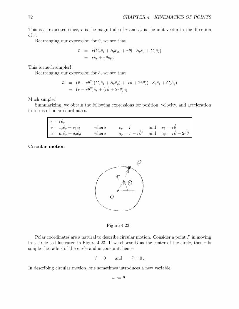
Circular motion
Figure 4.23:
Polar coordinates are a natural to describe circular motion. Consider a point P in movingin a circle as illustrated in Figure 4.23. If we choose O as the center of the circle, then r issimple the radius of the circle and is constant; hence
r = 0 and r = 0 .
In describing circular motion, one sometimes introduces a new variable
ω := θ .

4.4. PLANAR MOTION 73
Using the above expression for velocity in polar coordinates, we obtain that the velocity ofP is given by
v = veθ where v = rω .
Thus, the velocity of P is always tangential to the circle.
Figure 4.24: Velocity for circular motion
Noting that θ = ω and using the above above expression for acceleration in polar coor-dinates, we obtain that the acceleration of P is given by
a = arer + aθeθ where ar = −rω2 and aθ = rω
So the acceleration has both a radial and a tangential component. Since v = rw, we mayexpress the acceleration as
a = arer + aθeθ where ar = −v2
rand aθ = v
Uniform circular motion. Suppose P is moving counter-clockwise in a circle at constantspeed v. Then
v = 0
and
a = ar er where ar = −v2
r.
Thus, the acceleration of P is always towards the center of the circle. Sometimes this iscalled centripetal acceleration. The above expression also holds for clockwise motion.

74 CHAPTER 4. KINEMATICS OF POINTS
Figure 4.25: Acceleration for uniform circular motion
4.5 General three-dimensional motion
4.5.1 Cartesian coordinates
r = xe1 + ye2 + ze3
4.5.2 Cylindrical coordinates
ρ, θ, z
4.5.3 Spherical coordinates
r, θ, φ

Chapter 5
Kinematics of Reference Frames
5.1 Introduction
So far we have considered the kinematics of particles and points. Here we consider thekinematics of rigid bodies and reference frames.
A rigid body is a body which has the property that the distance between every two particlesof the body is constant with time.
Although a rigid body is an idealized concept, it is a very useful concept in studying themotion of real bodies such as aircraft and spacecraft. To study the kinematics of a rigidbody, we need only look at the kinematics of a reference frame in which the body is fixed;we call this a body fixed reference frame.
Figure 5.1: Body fixed frame
As we shall see shortly, the study of reference frame motion is also very useful in lookingat the motion of points.
5.2 A classification of reference frame motions
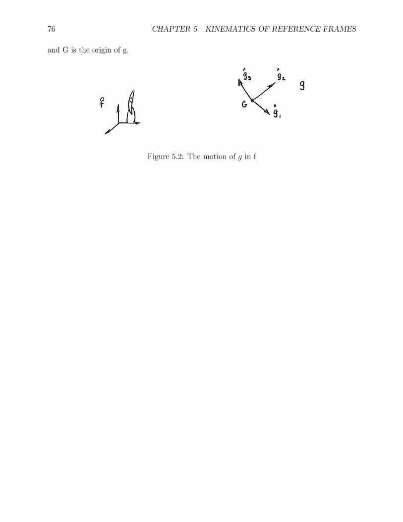
Consider the motion of a reference frame g relative to another reference frame f. Suppose
g = (g1, g2, g3)
75
76 CHAPTER 5. KINEMATICS OF REFERENCE FRAMES
and G is the origin of g.
Figure 5.2: The motion of g in f

5.2. A CLASSIFICATION OF REFERENCE FRAME MOTIONS 77
Translation. The motion of g in f is a translation or g translates in f if the directionsof g1, g2, g3 are constant in f.
Figure 5.3: A translation
Thus, a translation can be completely characterized by the motion of the origin of g; hencethe kinematics of translations can be completely described by the kinematics of points. Atranslation is said to be a rectilinear translation if the motion of the origin of g is rectilinear.
Figure 5.4: A rectilinear translation
Rotation. The motion of g in f is a rotation or g rotates in f if the origin of g is fixedin f. The motion of g in f is a simple rotation if there if a line L containing the origin of gwhich is fixed in both f and g.
With regard to the above definition, we call L the axis of rotation and say that g rotatesabout L.

78 CHAPTER 5. KINEMATICS OF REFERENCE FRAMES
Figure 5.5: A simple rotation
Fact. Any rotation can be decomposed into at most three simple rotations.
To illustrate the above fact consider the motion of g in f in the following picture where gis fixed in the bar. The motion of g in f is a rotation but it is not a simple rotation. Supposeone introduces a reference frame d which is fixed in the disc. Then the motion of g in f canbe considered a composition of the motion of d in f followed by the motion of g in d. Thelatter two motions are simple rotations. Thus the motion of g in f is a composition of twosimple rotations.
Figure 5.6: A composition of two simple rotations
General Reference Frame Motions. Any reference frame motion can be decomposedinto a translation and a rotation.
The above fact is illustrated by the motion of g in f in the following picture where g isfixed in the wheel. The motion of g in f is neither a translation nor a rotation. Suppose oneintroduces reference frame a which translates in f and whose origin is at the wheel center.Then the motion of g in f can be considered a composition of the motion of a in f and themotion of g in a, that is, it is a composition of a translation and a simple rotation.
5.3. MOTIONS WITH SIMPLE ROTATIONS 79
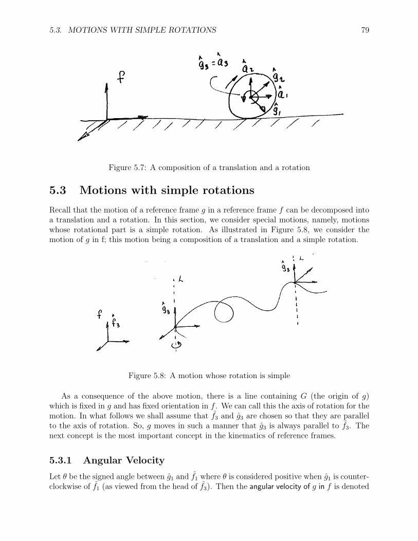
Figure 5.7: A composition of a translation and a rotation
5.3 Motions with simple rotations
Recall that the motion of a reference frame g in a reference frame f can be decomposed intoa translation and a rotation. In this section, we consider special motions, namely, motionswhose rotational part is a simple rotation. As illustrated in Figure 5.8, we consider themotion of g in f; this motion being a composition of a translation and a simple rotation.
Figure 5.8: A motion whose rotation is simple
As a consequence of the above motion, there is a line containing G (the origin of g)which is fixed in g and has fixed orientation in f . We can call this the axis of rotation for themotion. In what follows we shall assume that f3 and g3 are chosen so that they are parallelto the axis of rotation. So, g moves in such a manner that g3 is always parallel to f3. Thenext concept is the most important concept in the kinematics of reference frames.
5.3.1 Angular Velocity
Let θ be the signed angle between g1 and f1 where θ is considered positive when g1 is counter-clockwise of f1 (as viewed from the head of f3). Then the angular velocity of g in f is denoted

80 CHAPTER 5. KINEMATICS OF REFERENCE FRAMES
Figure 5.9: Angular velocity
by f ω g and is defined byf ω g = θf3 = θg3
Note that f ωg is a vector and is parallel to the axis of rotation of the motion. Forpractical purposes its direction can be determined by the right-hand rule. The quantity θ iscalled a rate of rotation and the angular speed of g in f is defined as | f ωg| = |θ|.
If g translates in f , then f ωg = 0.
dim [ f ωg] = T−1
units: rad s−1, rev min−1
Fact. Suppose B is a rigid body and g and h are any two reference frames fixed in B. Then,for any reference frame f , we have f ωh = f ωg The above fact leads to the following definitionfor a rigid body B.
Definition 1 The angular velocity of rigid body B in f is
f ωB := f ωg
where g is any reference frame fixed in B.
Example 18 When viewed from above, a vinyl record R rotates clockwise at a the rateω = 331
3rev/min. If reference frame f is fixed in the base of the record player, then
f ωR = −ωf3
where
ω = 331
3rev min−1 =
(3313)(2πrad)
60sec= 3.491rad sec−1 .

5.4. THE BASIC KINEMATIC EQUATION (BKE) 81
Figure 5.10: Vinyl time
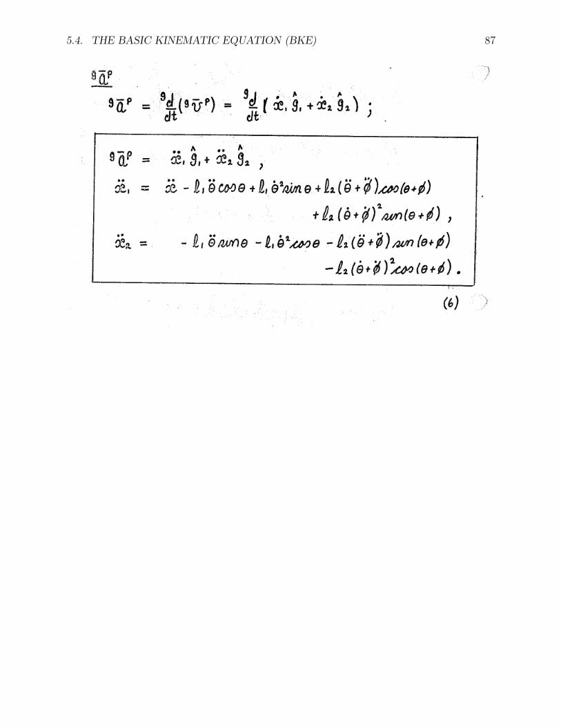
5.4 The Basic Kinematic Equation (BKE)
Suppose Z is any vector function of a scalar variable t and f and g are any two reference
frames. Suppose that we are interested in f ˙Z, the derivative of Z in f , but for some reason
Figure 5.11: BKE
or other, it is more convenient to obtain g ˙Z, the derivative of Z in g. Can we relate g ˙Z tof ˙Z? For the special motions considered in this section, the following theorem yields such adesired relationship.
Theorem 1 (Basic Kinematic Equation (BKE)) If Z is any vector function of a scalarvariable t, then
f ˙Z = g ˙Z +f ωg × Z
Before looking at a proof of this result, let us look at some examples which illustratethe use of the BKE. These are problems which we have previously solved without using theBKE.

82 CHAPTER 5. KINEMATICS OF REFERENCE FRAMES
Example 19 (Pendulum with moving support) Given:
l = 1ft , h = −2ft/sec (constant) , θ(t) = π/2 + t2rad
Find: evP and eaP at t = 0 sec.
Figure 5.12: Pendulum with moving support
Solution:
5.4. THE BASIC KINEMATIC EQUATION (BKE) 83
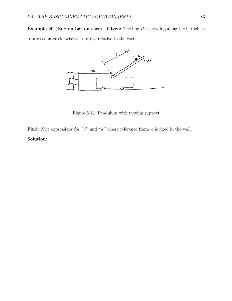
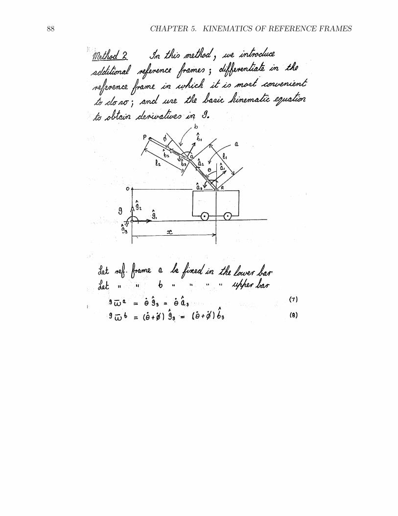
Example 20 (Bug on bar on cart) Given: The bug P is crawling along the bar which
rotates counter-clocwise at a rate ω relative to the cart.
Figure 5.13: Pendulum with moving support
Find: Nice expressions for evP and eaP where reference frame e is fixed in the wall.
Solution:

84 CHAPTER 5. KINEMATICS OF REFERENCE FRAMES

5.4. THE BASIC KINEMATIC EQUATION (BKE) 85

86 CHAPTER 5. KINEMATICS OF REFERENCE FRAMES
5.4. THE BASIC KINEMATIC EQUATION (BKE) 87
88 CHAPTER 5. KINEMATICS OF REFERENCE FRAMES

5.4. THE BASIC KINEMATIC EQUATION (BKE) 89

90 CHAPTER 5. KINEMATICS OF REFERENCE FRAMES

5.4. THE BASIC KINEMATIC EQUATION (BKE) 91

92 CHAPTER 5. KINEMATICS OF REFERENCE FRAMES
5.4.1 Polar coordinates revisited
Recall that if we are studying the planar motion of a point P in a reference frame f , it issometimes convenient to describe the motion of the point with polar coordinates, r and θas illustrated. We previously derived expressions for v, the velocity of P in f , and a, the
Figure 5.14: Polar coordinates
acceleration of P in f , in terms of polar coordinates. Without the BKE, the derivation ofthese expressions was tedious. We now rederive these expressions using the BKE. This isone illustration of the usefulness of the BKE.
Figure 5.15: A useful reference frame for polar coordinates
We first introduce a new reference frame g which consists of the three mutually perpen-dicular unit vectors er, eθ, e3 as illustrated. Note that
fωg = θe3 .
The position of P relative to O is given by
r = rer .
To obtain the velocity of P in f , we use the BKE between reference frames f and g withZ = r to yield
v =fd
dt(rer) =
gd
dt(rer) + f ωg × (rer) .

5.4. THE BASIC KINEMATIC EQUATION (BKE) 93
Since er is fixed in g,gd
dt(rer) = rer .
Also,f ωg × (rer) = (θe3) × (rer) = rθeθ
Hence,v = rer + rθeθ .
To obtain the acceleration of P in f , we use the BKE between reference frames f and gwith Z = v to yield
a =fdv
dt=
gdv
dt+ f ωg × v .
Since er and eθ are fixed in g,
gdv
dt=
gd
dt(rer + rθeθ) = rer + (rθ + rθ)eθ
Also,f ωg × v = (θe3) × (rer + rθeθ) = rθeθ − rθ2er .
Hence,a = (r − rθ2)er + (rθ + 2rθ)eθ .
5.4.2 Proof of the BKE for motions with simple rotations
Consider two reference frames
f = (f1, f2, f3) and g = (g1, g2, g3)
and suppose that f3 and g3 are chosen so that g3 always has the same direction as f3.
Figure 5.16: Proof of BKE
Consider any vector Z. Since g1, g2, g3 constitute a basis, there is a unique triplet ofscalars Z1, Z2, Z3 such that
Z = Z1g1 + Z2g2 + Z3g3 . (5.1)

94 CHAPTER 5. KINEMATICS OF REFERENCE FRAMES
By definition,g ˙Z = Z1g1 + Z2g2 + Z3g3 . (5.2)
Utilizing (5.1) and (5.2), we obtain
f ˙Z =fd
dt(Z1g1 + Z2g2 + Z3g3)
= Z1g1 + Z2g2 + Z3g3 + Z1
fdg1
dt+ Z2
fdg2
dt+ Z3
fdg3
dt
= g ˙Z + Z1
fdg1
dt+ Z2
fdg2
dt+ Z3
fdg3
dt. (5.3)
To computef dgi
dtwe need to express gi in terms of the unit vectors of f .
g1 = Cθf1 + Sθf2
g2 = −Sθf1 + Cθf2
g3 = f3
Hence,
fdg1
dt= −θSθf1 + θCθf2 = θg2 (5.4a)
fdg2
dt= −θCθf1 − θSθf2 = −θg1 (5.4b)
fdg3
dt= 0 (5.4c)
Looking at equations (5.4) and noting that
f ωg = θf3 = θg3 ,
we obtain
f ωg × g1 = (θg3) × g1 = θg2 =fdg1
dt(5.5a)
f ωg × g2 = (θg3) × g2 = −θg1 =fdg2
dt(5.5b)
f ωg × g3 = (θg3) × g3 = 0 =fdg3
dt(5.5c)
It follows from (5.5) that
Z1
fdg1
dt+ Z2
fdg2
dt+ Z3
fdg3
dt= Z1(
f ωg × g1) + Z2(f ωg × g2) + Z3(
f ωg × g3)
= f ωg × (Z1g1 + Z2g2 + Z3g3)
= f ωg × Z . (5.6)

5.4. THE BASIC KINEMATIC EQUATION (BKE) 95
Substitute (5.6) into (5.3) to obtain
f ˙Z = g ˙Z + f ωg × Z
In a later section, we shall see that the BKE holds for arbitrary motions of g in f.
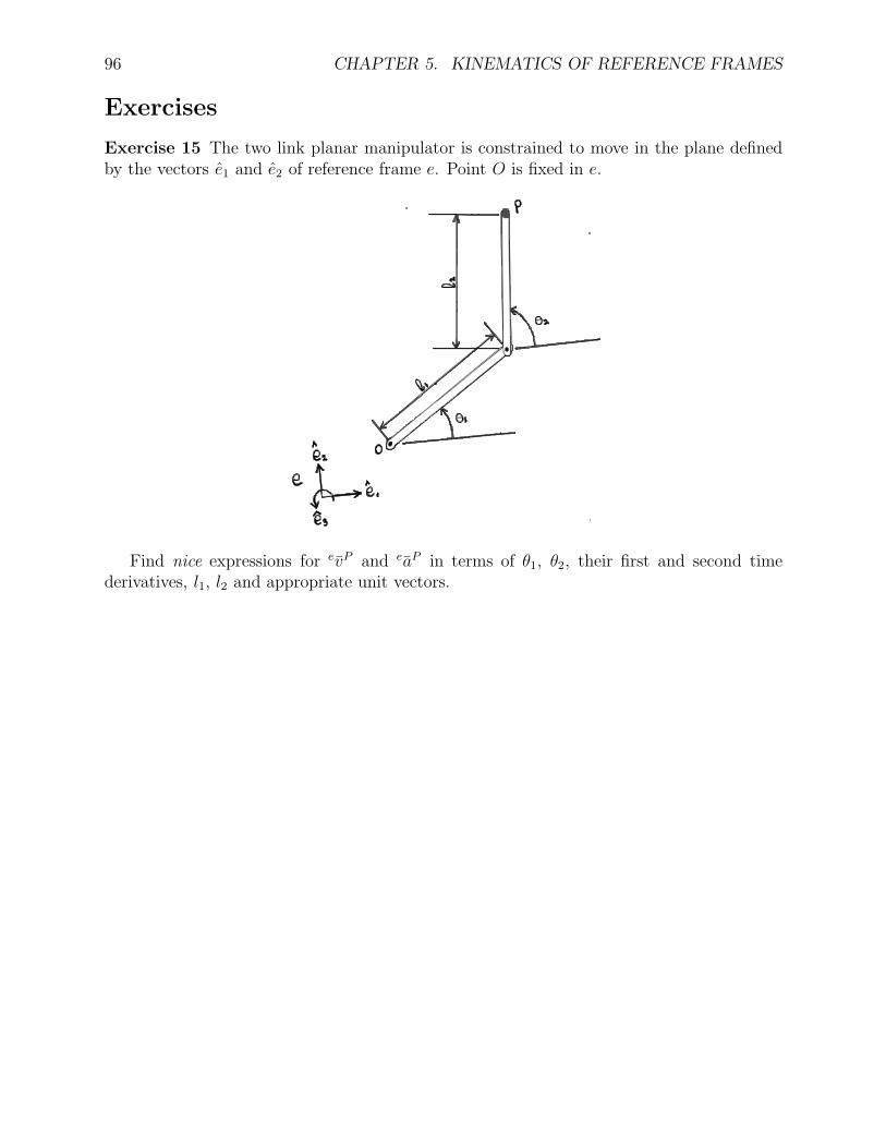
96 CHAPTER 5. KINEMATICS OF REFERENCE FRAMES
Exercises
Exercise 15 The two link planar manipulator is constrained to move in the plane definedby the vectors e1 and e2 of reference frame e. Point O is fixed in e.
Find nice expressions for evP and eaP in terms of θ1, θ2, their first and second timederivatives, l1, l2 and appropriate unit vectors.

5.4. THE BASIC KINEMATIC EQUATION (BKE) 97
Exercise 16 The small ball P moves in the straight slot which is fixed in the disk. Relativeto reference frame e, point O is fixed and the disk rotates about an axis through O which isparallel to e3 and perpendicular to the plane of the disk.
Find nice expressions for evP and eaP .
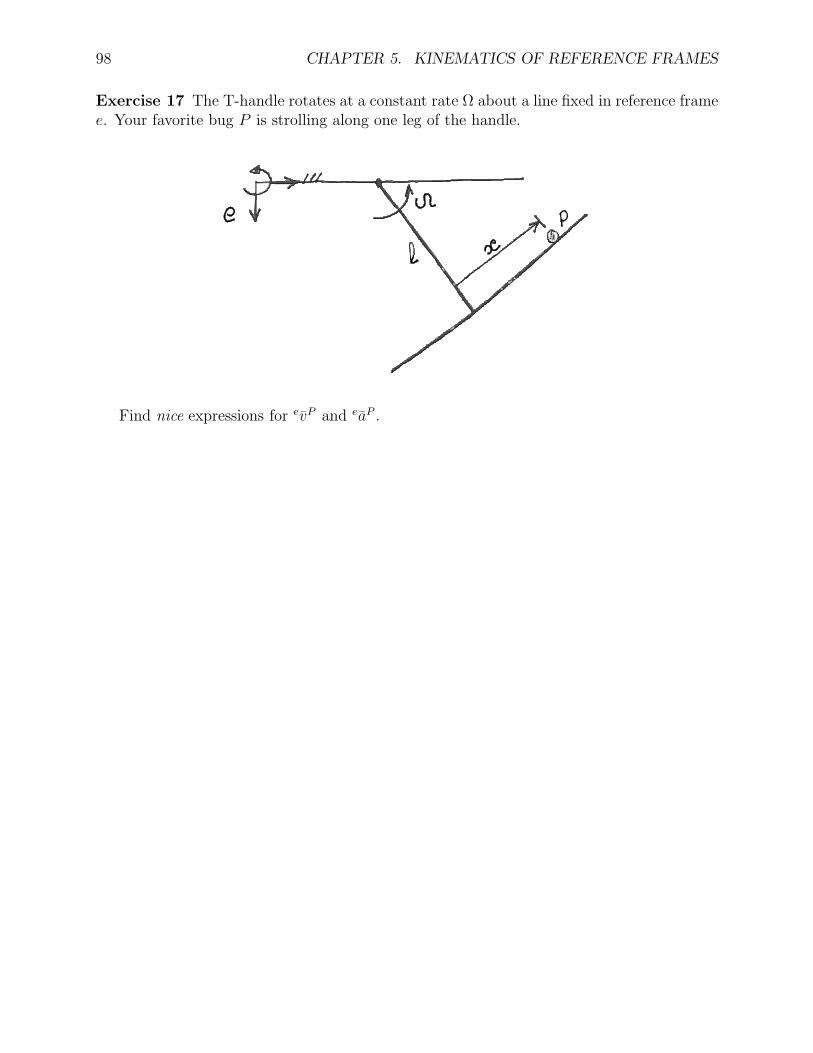
98 CHAPTER 5. KINEMATICS OF REFERENCE FRAMES
Exercise 17 The T-handle rotates at a constant rate Ω about a line fixed in reference framee. Your favorite bug P is strolling along one leg of the handle.
Find nice expressions for evP and eaP .

5.4. THE BASIC KINEMATIC EQUATION (BKE) 99
Exercise 18 Relative to reference frame e, the rigid frame A rotates at a constant rate rateΩ about a line passing through point O. Point P is moving along a line fixed in frame A.
Find nice expressions for evP and eaP .
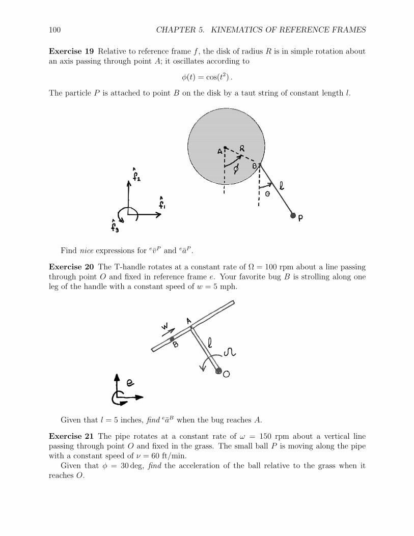
100 CHAPTER 5. KINEMATICS OF REFERENCE FRAMES
Exercise 19 Relative to reference frame f , the disk of radius R is in simple rotation aboutan axis passing through point A; it oscillates according to
φ(t) = cos(t2) .
The particle P is attached to point B on the disk by a taut string of constant length l.
Find nice expressions for evP and eaP .
Exercise 20 The T-handle rotates at a constant rate of Ω = 100 rpm about a line passingthrough point O and fixed in reference frame e. Your favorite bug B is strolling along oneleg of the handle with a constant speed of w = 5 mph.
Given that l = 5 inches, find eaB when the bug reaches A.
Exercise 21 The pipe rotates at a constant rate of ω = 150 rpm about a vertical linepassing through point O and fixed in the grass. The small ball P is moving along the pipewith a constant speed of ν = 60 ft/min.
Given that φ = 30 deg, find the acceleration of the ball relative to the grass when itreaches O.

5.4. THE BASIC KINEMATIC EQUATION (BKE) 101
Exercise 22 Relative to reference frame e, the large disk B rotates at a constant rate Ωabout an axis which passes through point O and is parallel to e3. The small disk A rotatesrelative to B at a constant rate ω about an axis which passes through point Q and is parallelto e3. Your favorite bug P is strolling along a radial line fixed in A.
Find nice expressions for evP and eaP .
Exercise 23 Relative to reference frame e, point P moves in the e1 − e2 plane with velocityv. Assuming v 6= 0, let uv be the unit vector in the direction of v; thus
v = vuv
Also let uφ be the unit vector which is 90 degrees counterclockwise from uv.Show that
eaP = vuv + vφuφ

102 CHAPTER 5. KINEMATICS OF REFERENCE FRAMES

Chapter 6
General Reference Frame Motions
Here we consider the general motion of a reference frame g as seen by another reference f .
Figure 6.1: General reference frame motions
6.1 Angular velocity
The angular velocity of a reference g in another reference frame f (denoted f ω g) can berigorously defined. Also the following property can be shown to hold.
If f , g, and h are any three reference frames, then
f ω h = f ω g + gω h
In other words, angular velocities add up like position vectors.
Example 21 Propeller on pitching aircraft
103

104 CHAPTER 6. GENERAL REFERENCE FRAME MOTIONS
Example 22 (Pitching and rolling aircraft.) Here θ is the pitch angle of the aircraftand φ is the roll angle.
Using the above property, one can obtain the following general property
If f 1, f 2, . . . , fn is any finite number of reference frames, then
f1ω fn
= f1ω f2
+ f2ω f3
+ · · ·+ f(n−1)ω fn
This relationship is very useful for practical computation of angular velocities. Recallthat every rotation can be decomposed into at most three simple rotations. Since we knowhow to compute angular velocities for simple rotations, we can use the above relationship tocompute angular velocities for general rotations.

6.1. ANGULAR VELOCITY 105
Example 23

106 CHAPTER 6. GENERAL REFERENCE FRAME MOTIONS
6.2 The basic kinematic equation (BKE)
The basic kinematic equation (BKE) holds for any motion of g in f . Specifically, if Z is any
Figure 6.2: The Basic Kinematic Equation (BKE)
vector function of time t, then
fdZdt
=gdZdt
+ f ω g × Z

6.2. THE BASIC KINEMATIC EQUATION (BKE) 107
Example 24 (Point on rotating pendulum) Given: The angular speed Ω is constant.
Find: Nice expressions for evP and eaP where e is fixed in the ground.
Figure 6.3: Example 24
Solution:

108 CHAPTER 6. GENERAL REFERENCE FRAME MOTIONS
Example 25 Given: The bug P is at point B when θ = 90. Also, the speed w and theangular speeds ω and Ω are constant.
Find: evP and eaP when θ = 90 where e is fixed in the ground.
Figure 6.4: Example 25

6.2. THE BASIC KINEMATIC EQUATION (BKE) 109
Example 26

110 CHAPTER 6. GENERAL REFERENCE FRAME MOTIONS
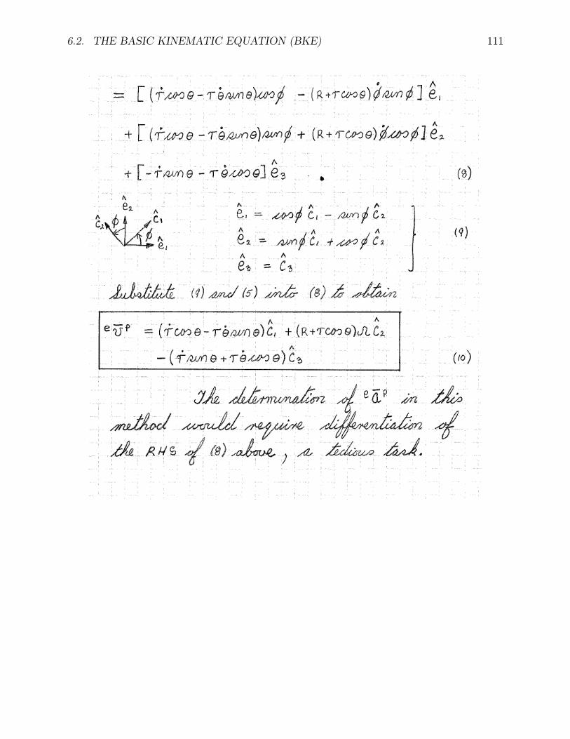
6.2. THE BASIC KINEMATIC EQUATION (BKE) 111

112 CHAPTER 6. GENERAL REFERENCE FRAME MOTIONS

6.2. THE BASIC KINEMATIC EQUATION (BKE) 113

114 CHAPTER 6. GENERAL REFERENCE FRAME MOTIONS

6.2. THE BASIC KINEMATIC EQUATION (BKE) 115

116 CHAPTER 6. GENERAL REFERENCE FRAME MOTIONS

Chapter 7
Angular Acceleration
Consider the motion of a reference frame g as seen by another reference frame f .
Figure 7.1: Angular acceleration
Angular acceleration is the time rate of change of angular velocity. The angular acceler-ation of g in f (denoted fα g) is defined as the time rate of change (in f) of the angularvelocity of g in f , that is,
fα g :=fd
dtfω g
If B is any rigid body and f is any reference frame, we denote the angular accelerationof B in f by fαB and define it to be equal to fαb where b is any reference frame fixed in B.
117

118 CHAPTER 7. ANGULAR ACCELERATION
Figure 7.2: Angular acceleration of a rigid body
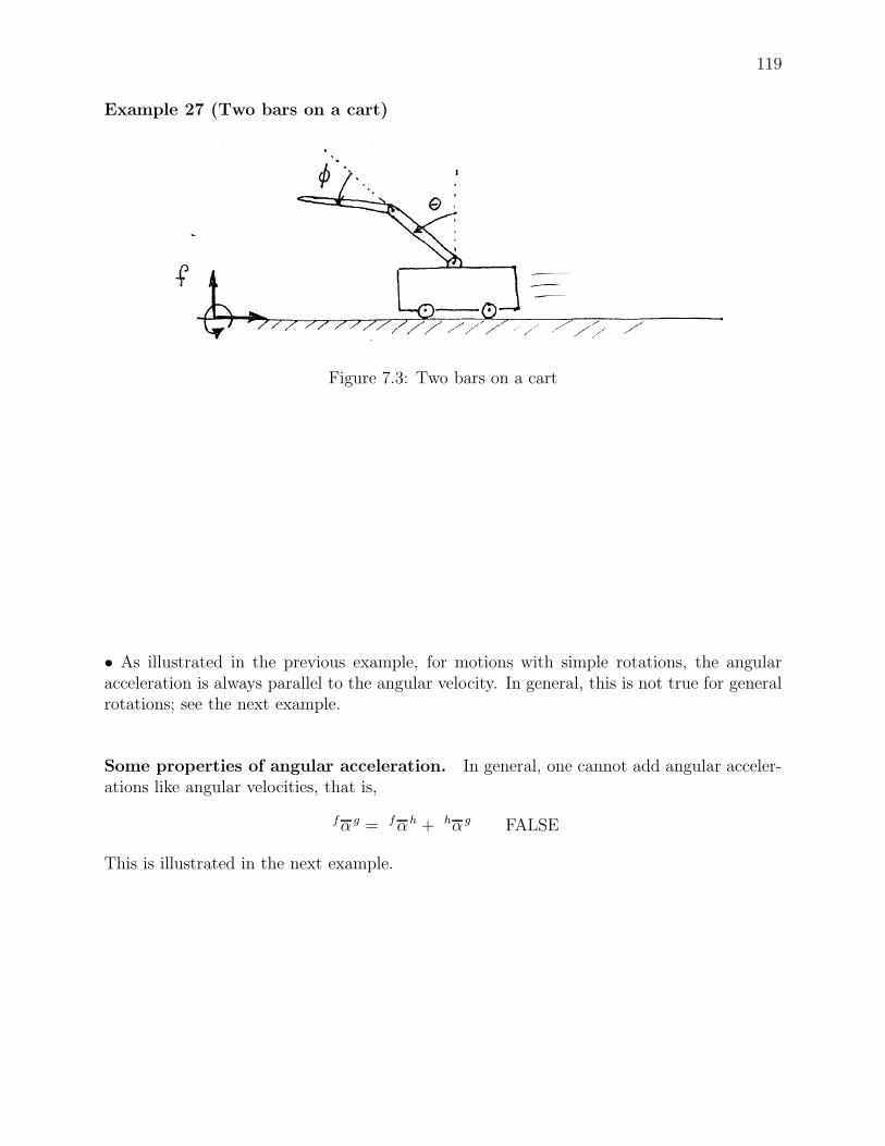
119
Example 27 (Two bars on a cart)
Figure 7.3: Two bars on a cart
• As illustrated in the previous example, for motions with simple rotations, the angularacceleration is always parallel to the angular velocity. In general, this is not true for generalrotations; see the next example.
Some properties of angular acceleration. In general, one cannot add angular acceler-ations like angular velocities, that is,
fα g = fαh + hα g FALSE
This is illustrated in the next example.

120 CHAPTER 7. ANGULAR ACCELERATION
Example 28 (Rotating pendulum) Find: An expression for the angular acceleration ofthe bar relative to the ground.
Figure 7.4: Rotating pendulum
Solution:
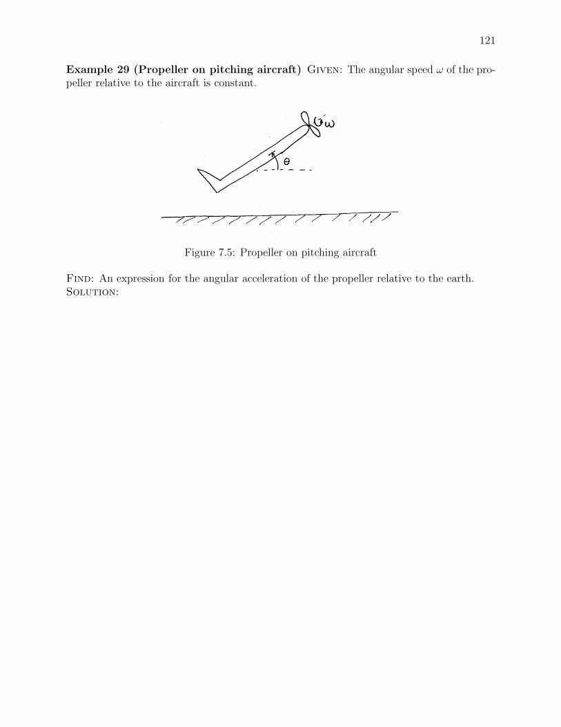
121
Example 29 (Propeller on pitching aircraft) Given: The angular speed ω of the pro-peller relative to the aircraft is constant.
Figure 7.5: Propeller on pitching aircraft
Find: An expression for the angular acceleration of the propeller relative to the earth.Solution:

122 CHAPTER 7. ANGULAR ACCELERATION
• Another property:
fα g =gd
dtfω g
The above relationship says that one can obtain fα g by differentiating fω g in the g frameinstead of the f frame. In other words, the rate of change of fω g is the same for the framesf and g. To see this, use the definition of fω g and the BKE to obtain:
fα g =fd
dtfω g
=gd
dtfω g + fω g × fω g
=gd
dtfω g

123
Example 30 (Arm on centrifuge) Given: The angular speed Ω of the centrifuge rela-tive to the ground is constant.
Figure 7.6: Arm on rotating centrifuge
• The rotation of c relative to e:
eωc = Ωe3 = Ωc3 .
Recalling that Ω is constant, we have
eαc =ed
dteωc =
ed
dt(Ωe3) = 0 .
• The rotation of a relative to c:cωa = θc2 = θa2 .
Hencecαa =
cd
dtcωa =
ed
dt
(
θc2
)
= θc2 .
• The rotation of a relative to e:
eωa = eωc + cωa = Ωe3 + θc2 = Ωc3 + θc2 .
Noticing that eωa can be expressed in terms of the vectors of c, we use the BKE to obtainthat
eαa =ed
dteωa
=cd
dteωa +eωc ×eωa (using BKE)
=cd
dt
(
θc2 + Ωc3
)
+ (Ωc3) × (θc2 + Ωc3)
= −Ωθc1 + θc2 .
Note thateαa 6= eαc + cαa .

124 CHAPTER 7. ANGULAR ACCELERATION
7.1 Exercises
Exercise 24
Exercise 25

Chapter 8
Kinematic Expansions
Figure 8.1: Kinematic expansions
8.1 The velocity expansion
Suppose we are interested in the velocity of a point P as seen by an observer in a reference f ,but, it is much easier to obtain the velocity of P relative to another reference frame g. Canwe relate f v P to gv P ? Yes, we can and that relationship is given by the velocity expansion(VE):
f v P = f v G + f ω g × r GP + gv P (8.1)
where G is any point which is fixed in reference frame g.Note that in applying the velocity expansion between f and g we must choose some
convenient point G which is fixed in g. Quite often, G is the origin of g.
Examples and proof of VE.
125

126 CHAPTER 8. KINEMATIC EXPANSIONS
Example 31 (Pendulum with moving support) Given:
l = 1ft , h = −2ft/sec (constant) , θ(t) = π/2 + t2rad
Find: evP at t = 0 sec.
Figure 8.2: Pendulum with moving support
Solution:
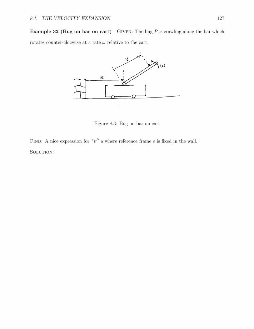
8.1. THE VELOCITY EXPANSION 127
Example 32 (Bug on bar on cart) Given: The bug P is crawling along the bar which
rotates counter-clocwise at a rate ω relative to the cart.
Figure 8.3: Bug on bar on cart
Find: A nice expression for evP a where reference frame e is fixed in the wall.
Solution:

128 CHAPTER 8. KINEMATIC EXPANSIONS
Example 33 (Point on rotating pendulum) Given: The angular speed Ω is constant.
Find: A nice expression for evP where e is fixed in the ground.
Figure 8.4: Example 33
Solution:

8.2. THE ACCELERATION EXPANSION 129
8.2 The acceleration expansion
The acceleration expansion (AE) does for accelerations what the velocity expansion does forvelocities. It is given by
f aP = f aG + f ω g × ( f ω g × r GP ) + f αg × r GP + 2 f ω g × gv P + ga P (8.2)
where G is any point which is fixed in reference frame g.
Examples and proof of AE.

130 CHAPTER 8. KINEMATIC EXPANSIONS
Example 34 (Pendulum with moving support) Given:
l = 1ft , h = −2ft/sec (constant) , θ(t) = π/2 + t2rad
Find: eaP at t = 0 sec.
Figure 8.5: Pendulum with moving support
Solution:

8.2. THE ACCELERATION EXPANSION 131
Example 35 (Bug on bar on cart) Given: The bug P is crawling along the bar which
rotates counter-clocwise at a rate ω relative to the cart.
Figure 8.6: Bug on bar on cart
Find: A nice expression for eaP where reference frame e is fixed in the wall.
Solution:

132 CHAPTER 8. KINEMATIC EXPANSIONS
Example 36 (Point on rotating pendulum) Given: The angular speed Ω is constant.
Find: Using the acceleration expansion, find a nice expression for eaP where e is fixed in theground.
Figure 8.7: Example 36
Solution:
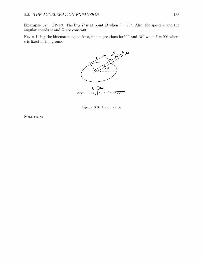
8.2. THE ACCELERATION EXPANSION 133
Example 37 Given: The bug P is at point B when θ = 90. Also, the speed w and theangular speeds ω and Ω are constant.
Find: Using the kinematic expansions, find expressions for evP and eaP when θ = 90 wheree is fixed in the ground.
Figure 8.8: Example 37
Solution:

134 CHAPTER 8. KINEMATIC EXPANSIONS
8.3 Exercises
Exercise 26
Exercise 27

8.3. EXERCISES 135
Exercise 28
Exercise 29 The disk rotates about a vertical axis through point O at a constant rate Ω.The small bug P moves relative to a slot fixed in the disk at a constant speed v. Consideringa reference frame g fixed in the ground, find expressions for gvP and gaP at the instant Preaches point B.

136 CHAPTER 8. KINEMATIC EXPANSIONS

Chapter 9
Particle Dynamics
9.1 Introduction
So far, we have considered motion without considering the causes of motion. We considernow what causes the motions of bodies. We initially look at the simplest types of bodies,namely, particles. Recall that a particle is a body that occupies a single point in space at eachinstant of time. Of course, this is a convenient mathematical idealization. However, it is veryuseful in modelling a physical body whose size is very small in comparison to other significantsizes in the situation under consideration. Consider the motion of the earth about the sun.In this situation, a good first approximation of the earth would be a particle. However, instudying the motion of an aircraft near the surface of the earth, a particle model of the earthis no longer useful. The point a particle occupies is called its position (or location). To studyhow motions are caused we need the concepts of mass and force.
The mass of a body is “a measure of its resistance to change in motion.” The mass of abody is the same throughout the universe. Do not confuse the concepts of mass and weight.Mass is a positive scalar quantity. Its dimension is indicated by M and the SI and US unitsare kilogram (kg) and slug (slug), respectively.
Forces are the interactions between bodies. Every force is due to the interaction betweentwo bodies. For a given body, the forces exerted on it by other bodies cause its motion. Theeffect of a force depends not only its magnitude and direction but also on where it is applied.So, we model forces with bound vectors. A bound vector is a vector which is associated witha specific point of application.
Figure 9.1: Bound vector
The point of application of a force acting on a particle is the position of the particle. Thedimension of force is indicated by F . The SI and US units of force are the newton (N) andpound (lb), respectively, for example,
F = (e1 + 2e2 + 3e3) lb
137
138 CHAPTER 9. PARTICLE DYNAMICS
orF = (2e1 + 3e3) N .

9.2. NEWTON’S SECOND LAW 139
9.2 Newton’s second law
Consider a particle which is subject to a bunch of forces,
F 1, F 2, . . . , F N ,
as illustrated in Figure 9.2. Let ΣF be the resultant force acting on the particle, that is, itis the sum of all the forces acting on the particle. So,
ΣF = F 1 + F 2 + . . . + F N =N∑
j=1
F j
Figure 9.2: Newton’s second law
Sometimes Newton’s second law is stated as follows: In an inertial reference frame, theacceleration of a particle is always proportional to the resultant force on the particle. Thisproportionality constant m is called the mass of the particle. So, we have
ΣF = ma
where a is the acceleration of the particle in an inertial reference frame. The problem withthe above statement is that it introduces the undefined notion of an inertial reference frame.Another way to approach Newton’s second law is first to define an inertial reference frameas any reference frame for which ΣF = ma always holds and then simply state Newton’ssecond law as:
There exists an inertial reference frame.
Practical inertial reference frames. For many everyday problems and problems in me-chanical and civil engineering, a reference frame in which the earth is fixed can be consideredinertial. However, in many aerospace situations, for example, a satellite orbiting the earth,one must use as inertial a reference frame with origin at the center of the earth and withrespect to which the earth rotates at a rate of one revolution per day. If one is studying themotion of the earth relative to the sun, one must consider a reference fixed in the sun asinertial.
140 CHAPTER 9. PARTICLE DYNAMICS
If f is an inertial reference frame and g is a reference frame which translates with constantvelocity in f , then gaP = f aP ; hence g is also inertial.
ΣF = ma is not good for speeds close to the speed of light. In these situations, one mustresort to relativistic mechanics.
From ΣF = ma, we must have
F = MLT−2
1N = 1 kgms−2
1 slug = 1 lb sec2 ft−1
Suppose b1, b1, b1 are three basis vectors which are not necessarily orthogonal to eachother and are not necessarily fixed in an inertial frame. Considering components relative tothis basis, we have
a = a1b1 + a2b2 + a3b3
andΣF = (ΣF1) b1 + (ΣF2) b2 + (ΣF3) b3
where, for i = 1, 2, 3, the scalar ΣFi is the sum of the components in the bi direction of allthe forces acting on the particle. Hence we obtain the following three scalar equations:
ΣF1 = ma1
ΣF2 = ma2
ΣF3 = ma3
Basically, these equations state that the resultant force in the i-th direction equals the masstimes the acceleration in that direction.
9.3 Static equilibrium
A particle P is in static equilibrium if it is at rest in some inertial reference frame; that is,f vP = 0 where f is inertial
Result. If a particle is in static equilibrium, then the sum of all the forces acting on theparticle is zero, that is,
ΣF = 0
Proof. Since the particle is at rest in an inertial reference frame, its acceleration a in thatframe is zero. The above result now follows from ΣF = ma .
Suppose b1, b1, b1 are three basis vectors which are not necessarily orthogonal to eachother and are not necessarily fixed in an inertial frame. Considering components relative tothis basis, we have
ΣF = (ΣF1) b1 + (ΣF2) b2 + (ΣF3) b3

9.4. NEWTON’S THIRD LAW 141
where, for i = 1, 2, 3, the scalar ΣFi is the sum of the components in the bi direction of allthe forces acting on the particle. Hence we obtain the following three scalar equations:
ΣF1 = 0ΣF2 = 0ΣF3 = 0
Basically, these equations state that the resultant force in the i-th direction equals zero.
9.4 Newton’s third law
Newtons Third Law has two parts:
(a) If a body A exerts a force F on another body B, then the second body B exerts a force−F on the first body A which is equal in magnitude but opposite in direction to F .
Sometimes this is loosely stated as “action and reaction are equal but opposite”.
Figure 9.3: Newton’s third law: first part
(b) If A and B are particles then, the forces F and −F are along the line joining the twoparticles.
Figure 9.4: Newton’s third law: second part
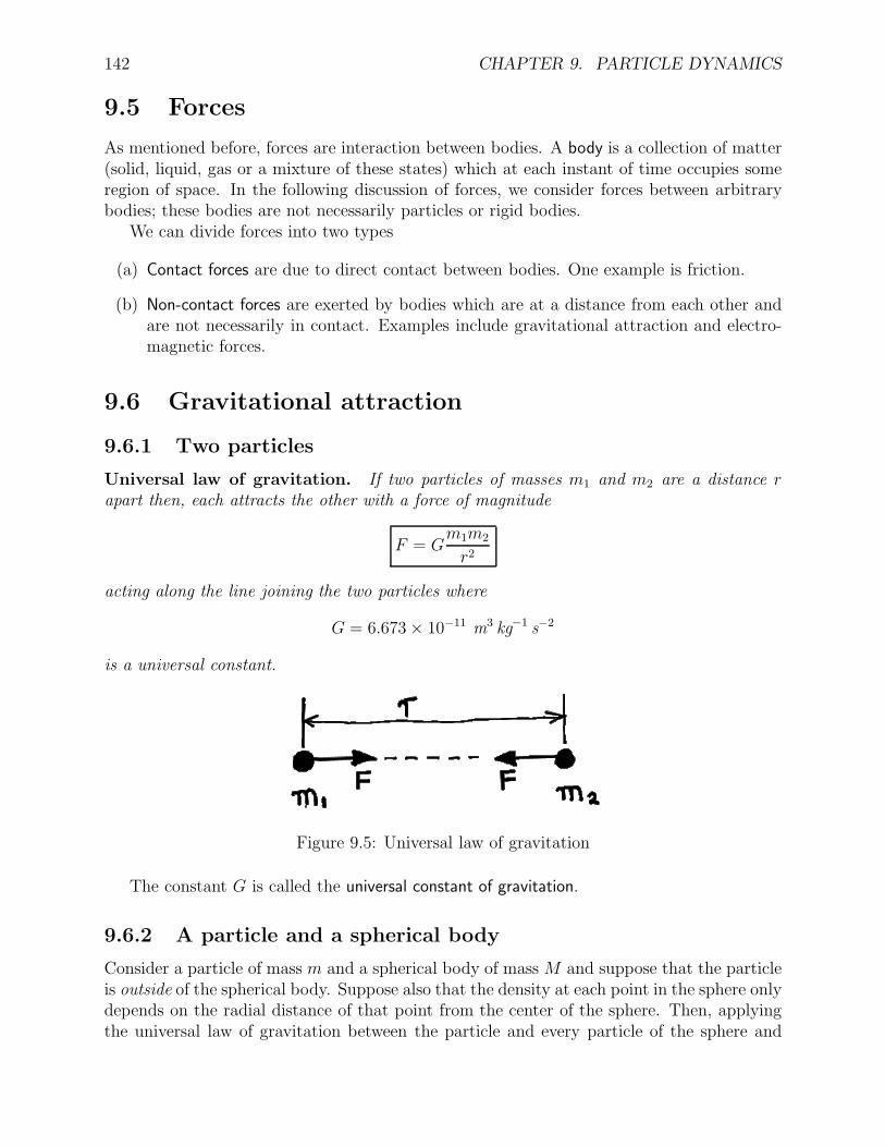
142 CHAPTER 9. PARTICLE DYNAMICS
9.5 Forces
As mentioned before, forces are interaction between bodies. A body is a collection of matter(solid, liquid, gas or a mixture of these states) which at each instant of time occupies someregion of space. In the following discussion of forces, we consider forces between arbitrarybodies; these bodies are not necessarily particles or rigid bodies.
We can divide forces into two types
(a) Contact forces are due to direct contact between bodies. One example is friction.
(b) Non-contact forces are exerted by bodies which are at a distance from each other andare not necessarily in contact. Examples include gravitational attraction and electro-magnetic forces.
9.6 Gravitational attraction
9.6.1 Two particles
Universal law of gravitation. If two particles of masses m1 and m2 are a distance rapart then, each attracts the other with a force of magnitude
F = Gm1m2
r2
acting along the line joining the two particles where
G = 6.673 × 10⁻¹¹ m3 kg−1 s−2
is a universal constant.
Figure 9.5: Universal law of gravitation
The constant G is called the universal constant of gravitation.
9.6.2 A particle and a spherical body
Consider a particle of mass m and a spherical body of mass M and suppose that the particleis outside of the spherical body. Suppose also that the density at each point in the sphere onlydepends on the radial distance of that point from the center of the sphere. Then, applyingthe universal law of gravitation between the particle and every particle of the sphere and

9.6. GRAVITATIONAL ATTRACTION 143
integrating over the sphere one can show that the gravitational attraction of the sphere onthe particle is equivalent to that of a particle of mass M located at the center of the sphere.Thus, the resultant force exerted by the sphere on the particle has magnitude
F = GMm
r2
where r is the distance of the particle from the center of the sphere. This force is along theline joining the particle to the sphere center and is directed towards the sphere center.
Figure 9.6: Gravitational attraction of a sphere on a particle
9.6.3 A particle and the earth
Suppose we model the earth as a spherical body. Then, the gravitational attraction of theearth on a particle above earth is equivalent to that of a particle of mass M⊕ located at thecenter of earth where M⊕ is the mass of the earth and is given by
M⊕ = 5.976×1024 kg .
Thus, the magnitude F of the resultant force exerted by the earth on a particle above theearth is given by
F = GM⊕m
r2
where r is the distance of the particle from the center of the earth. This force is along theline joining the particle to the center of the earth and is directed towards the center of theearth.
Weight. If a particle is close to or on the surface of the earth then, r ≈ R⊕ where R⊕ isthe mean radius of the earth and is given by
R⊕ = 6.371×10⁶ m .
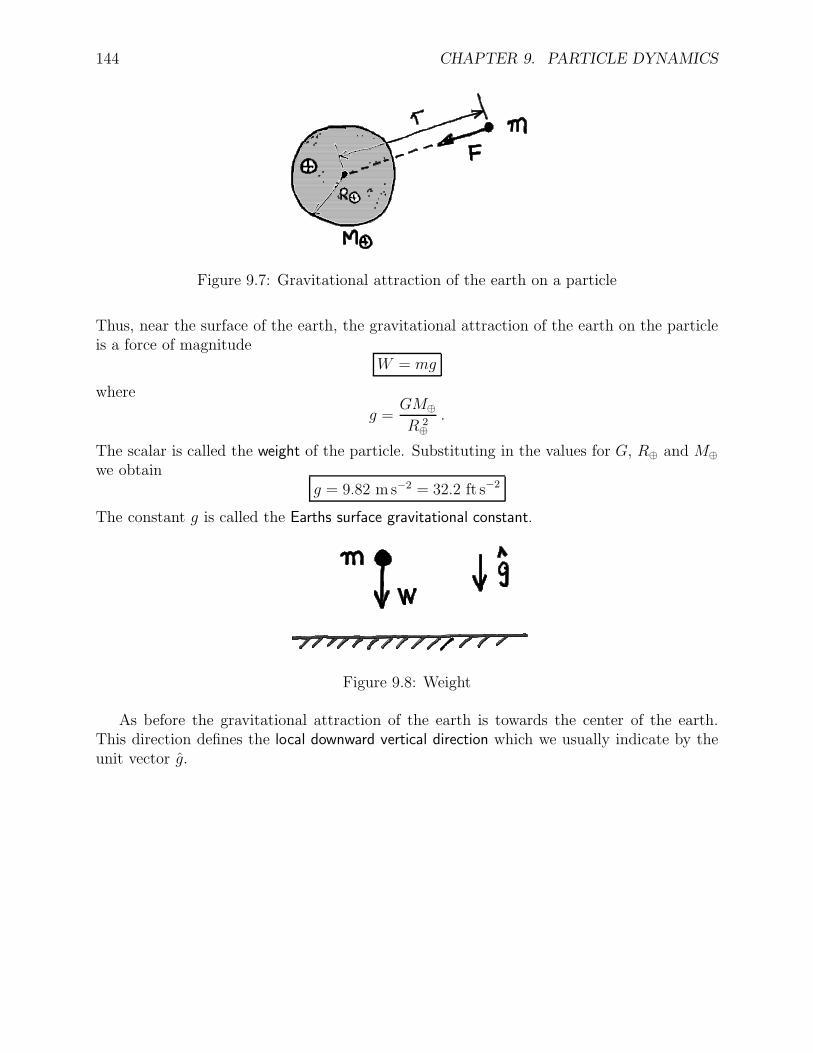
144 CHAPTER 9. PARTICLE DYNAMICS
Figure 9.7: Gravitational attraction of the earth on a particle
Thus, near the surface of the earth, the gravitational attraction of the earth on the particleis a force of magnitude
W = mg
where
g =GM⊕
R 2⊕
.
The scalar is called the weight of the particle. Substituting in the values for G, R⊕ and M⊕we obtain
g = 9.82 m s−2 = 32.2 ft s−2
The constant g is called the Earths surface gravitational constant.
Figure 9.8: Weight
As before the gravitational attraction of the earth is towards the center of the earth.This direction defines the local downward vertical direction which we usually indicate by theunit vector g.

9.7. CONTACT FORCES 145
9.7 Contact forces
We idealize a contact force by idealizing the body exerting that force.
9.7.1 Strings
We idealize ropes, cables, etc., as strings.
A string is a one-dimensional body. When it is taut and attached to another body, itexerts a force whose direction is tangential to the string and into the string at the pointof attachment. If the string is not taut then, the force exerted by the string is zero. Themagnitude of the force exerted by a string is called the tension in the string.
Thus, a string pulls, but never pushes. Also, the direction of the force it exerts iscompletely determined by the string geometry. For a straight string, the force exerted bythe string is parallel to the string and into the string.
Mathematically, we can represent a force T due to a string as
T = T u
where T is the tension in the string and the unit vector u is tangential to the string and intothe string at the point of attachment.
Figure 9.9: Straight strings
Figure 9.10: Curved strings

146 CHAPTER 9. PARTICLE DYNAMICS
Example 38 Given: The block of weight W = 10 lb is supported by two cables as shown.
Figure 9.11: Example 38
Find: the tension in each cable at the block.Solution:

9.7. CONTACT FORCES 147
Example 39 Given: The ball of mass m = 5 kg is supported by two cables as shown.
Figure 9.12: Example 39
Find: the tension in each cable at the ball.Solution:

148 CHAPTER 9. PARTICLE DYNAMICS
Example 40 Given: The ball is supported by a string and moves in a circle of radiusR = 0.25 m at a speed of 10 m/s.
Figure 9.13: Example 40
Find: φSolution:

9.7. CONTACT FORCES 149
Example 41 Given: The ball is supported by two strings and moves in a circle of radiusR = 1/2 m with φ = 45.
Figure 9.14: Example 41
Find: Minimum value of v.Solution:

150 CHAPTER 9. PARTICLE DYNAMICS

9.7. CONTACT FORCES 151
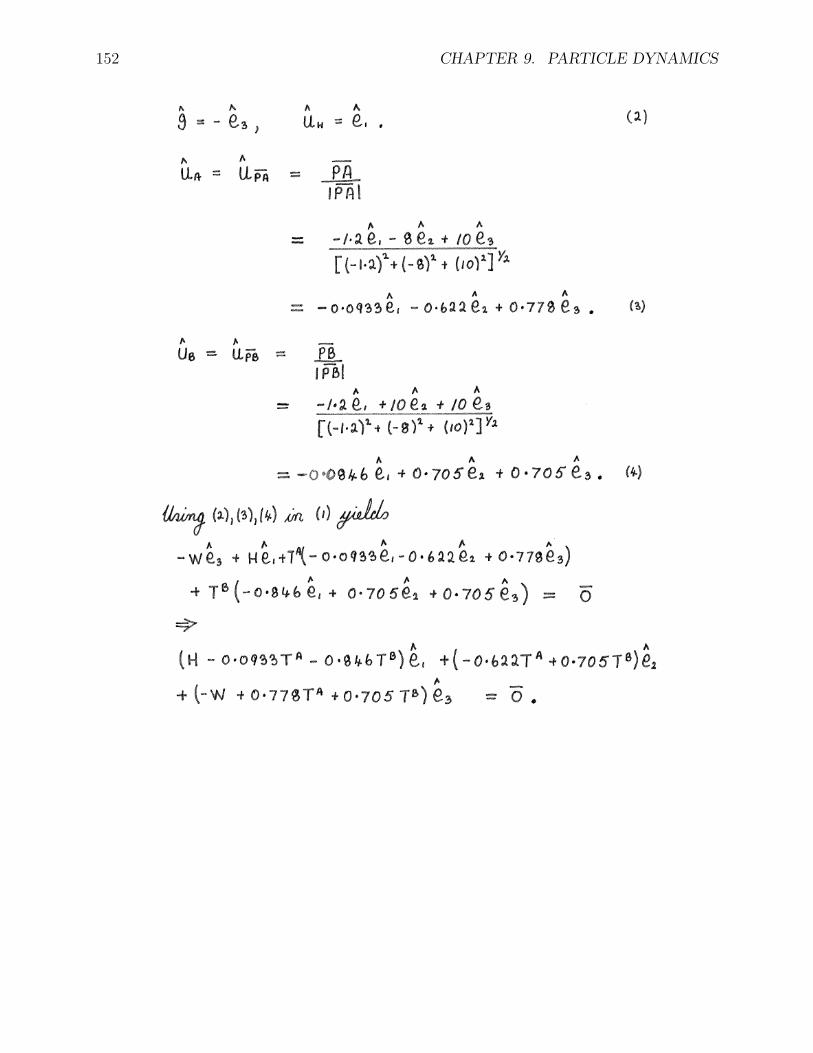
152 CHAPTER 9. PARTICLE DYNAMICS

9.7. CONTACT FORCES 153

154 CHAPTER 9. PARTICLE DYNAMICS
9.8 Application of ΣF = ma
9.8.1 Free body diagrams
In order to reliably model the forces on a given body, a free body diagram (FBD) is drawn.A free body diagram of a body is a picture containing the body and all the external forcesacting on the body. All other bodies are replaced by the forces they exert on the given body.
A FBD should be drawn before applying ΣF = ma.
The FBD should contain all available information on the forces. All forces should be labeled.
9.8.2 A systematic procedure
The following is a systematic procedure for applying ΣF = ma to obtain scalar equations.
(a) Obtain the inertial acceleration a. In static problems, this is trivial because a = 0.
(b) Model all the forces on the body. A free body diagram is needed at this step.
(c) Introduce a set of basis vectors and resolve the acceleration and all the forces intocomponents relative to this basis.
(d) Apply ΣF = ma.
(e) Obtain scalar equations.
Sometimes step (c) is performed as part of step (e).
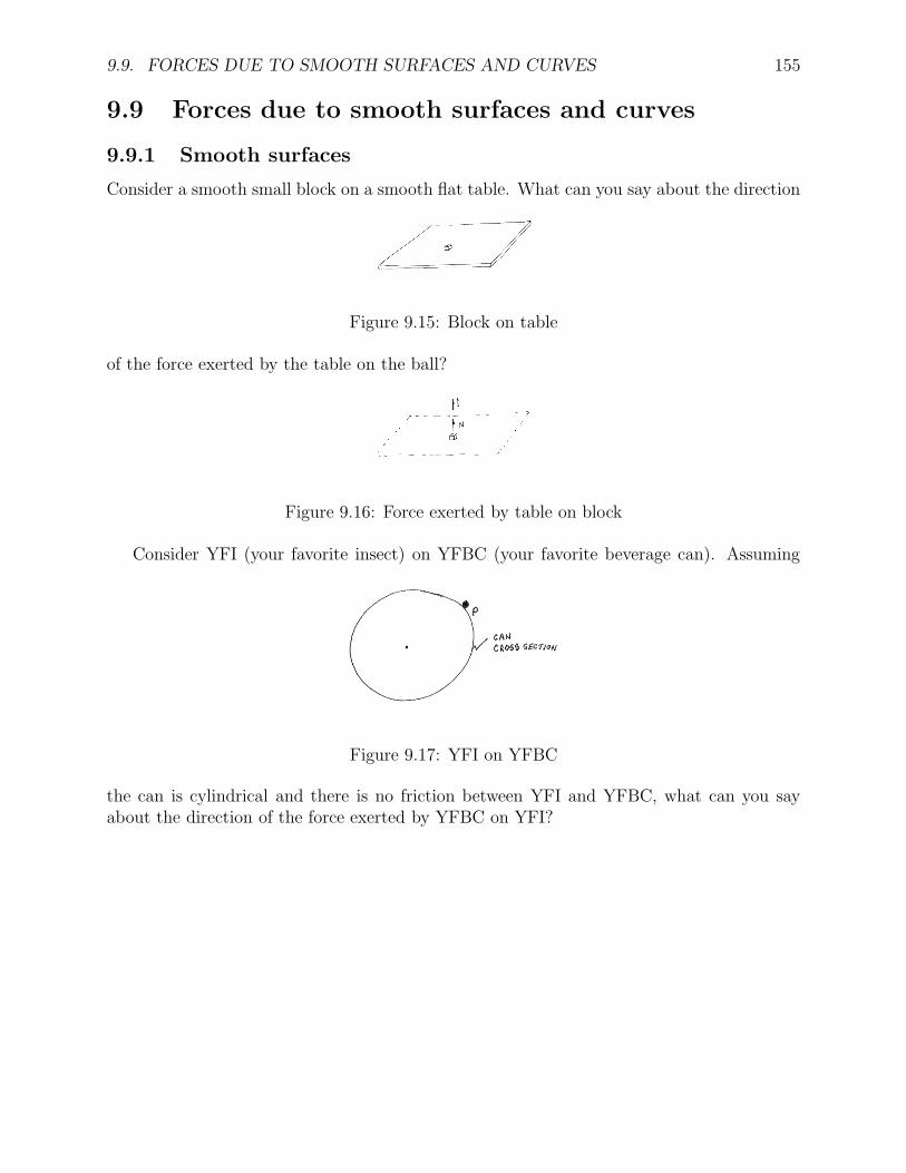
9.9. FORCES DUE TO SMOOTH SURFACES AND CURVES 155
9.9 Forces due to smooth surfaces and curves
9.9.1 Smooth surfaces
Consider a smooth small block on a smooth flat table. What can you say about the direction
Figure 9.15: Block on table
of the force exerted by the table on the ball?
Figure 9.16: Force exerted by table on block
Consider YFI (your favorite insect) on YFBC (your favorite beverage can). Assuming
Figure 9.17: YFI on YFBC
the can is cylindrical and there is no friction between YFI and YFBC, what can you sayabout the direction of the force exerted by YFBC on YFI?

156 CHAPTER 9. PARTICLE DYNAMICS
Figure 9.18: Force exerted by YFBC on YFI
Consider now the general situation of a particle in contact with a smooth surface. By asurface, we mean a 2-dimensional geometric object such as a plane or the “surface” of acylinder. At every point on a surface (except at corners), there is a well defined line whichpasses through the point and is normal (perpendicular) to the surface at the point.
Figure 9.19: Particle on a surface
The force exerted by a smooth surface on a particle in contact with the surface is normalto the surface at the point of contact and is directed towards the particle. (Surfaces don’tsuck.) We can represent this by
N = Nu N ≥ 0
where the unit vector u is normal to the surface at the location of the particle and is directedtowards the particle . Thus the direction of the force exerted by a smooth surface is com-
Figure 9.20: Normal force due to a surface
pletely determined by the surface geometry and the location of the particle. This force iscalled a normal force.

9.9. FORCES DUE TO SMOOTH SURFACES AND CURVES 157
Example 42 Given: The block of mass m = 2 kg lies on a smooth inclined plane (Θ = 30)and is attached to the wall via a string.Find: The tension in the string.
Figure 9.21: Example 42
Solution:
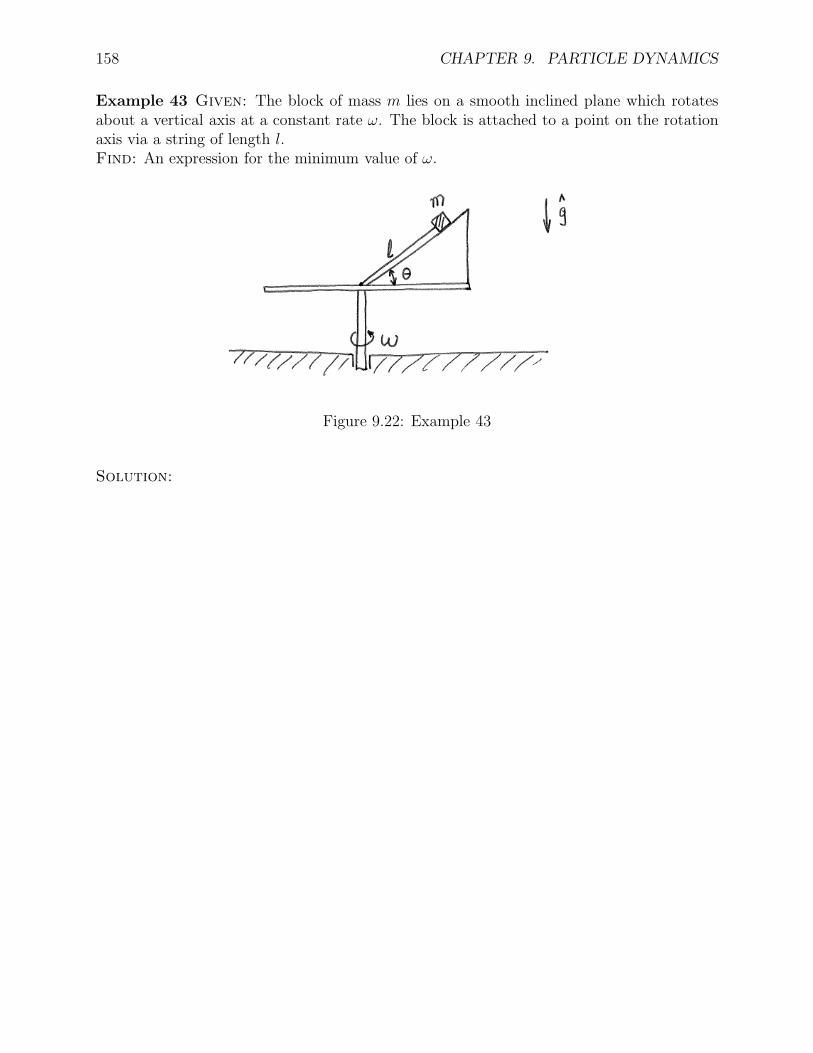
158 CHAPTER 9. PARTICLE DYNAMICS
Example 43 Given: The block of mass m lies on a smooth inclined plane which rotatesabout a vertical axis at a constant rate ω. The block is attached to a point on the rotationaxis via a string of length l.Find: An expression for the minimum value of ω.
Figure 9.22: Example 43
Solution:

9.9. FORCES DUE TO SMOOTH SURFACES AND CURVES 159
9.9.2 Smooth curves
Consider a smooth bead constrained to move along a smooth straight wire.
Figure 9.23: Smooth bead on smooth wire
What can you say about the force exerted by the wire on the bead? The force exerted bythe wire on the bead is in the plane which is perpendicular or normal to the wire.
Figure 9.24: Force exerted by wire on bead
Consider a smooth small ball constrained to move inside a smooth circular tube . What
Figure 9.25: Smooth ball in smooth tube
can you say about the force exerted by the tube on the ball? The force exerted by the tubeon the ball is in the plane which is perpendicular or normal to the line which is tangent tothe tube at the ball’s location.

160 CHAPTER 9. PARTICLE DYNAMICS
Figure 9.26: Force exerted by tube on ball
Consider now the general situation of a particle in contact with a curve. By a curve, wemean a one-dimensional geometric object such as a straight line or a circle. At every pointon a curve (except at corners), there is a well defined plane which passes through the pointand is normal (perpendicular) to the line which is tangent to the curve at the point. We saythat this plane is normal to the curve.
Figure 9.27: Particle in contact with a curve
The force N exerted by a smooth curve on a particle is normal to the curve at the positionof the particle, that is, it lies in the plane which is normal to the curve at the location of theparticle. We can represent this by
N = N2u2 + N3u3
where u2, u3 are any two independent unit vectors which are normal to the curve at thelocation of the particle
Note that in contrast to smooth surfaces, the direction of the force exerted by a smoothcurve is unknown. This force is called a normal force.

9.9. FORCES DUE TO SMOOTH SURFACES AND CURVES 161
Figure 9.28: Normal force due to a curve

162 CHAPTER 9. PARTICLE DYNAMICS
Example 44 Given: The smooth ball of mass m is being pulled by the string (of varyinglength l) relative to the smooth tube at a constant speed v. The tube rotates about a verticalaxis at a constant angular speed of ω.Find: Expressions for (a) the tension in the string (b) the force exerted by the tube on theball.
Figure 9.29: Example 44
Solution:
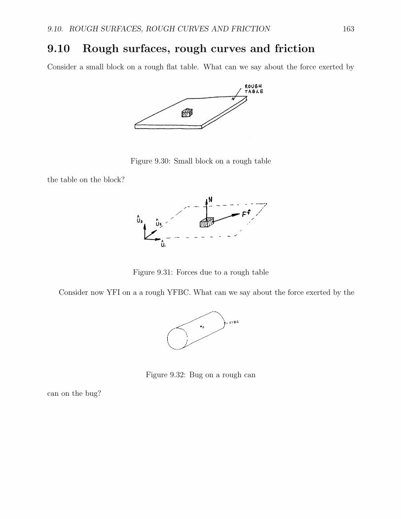
9.10. ROUGH SURFACES, ROUGH CURVES AND FRICTION 163
9.10 Rough surfaces, rough curves and friction
Consider a small block on a rough flat table. What can we say about the force exerted by
Figure 9.30: Small block on a rough table
the table on the block?
Figure 9.31: Forces due to a rough table
Consider now YFI on a a rough YFBC. What can we say about the force exerted by the
Figure 9.32: Bug on a rough can
can on the bug?
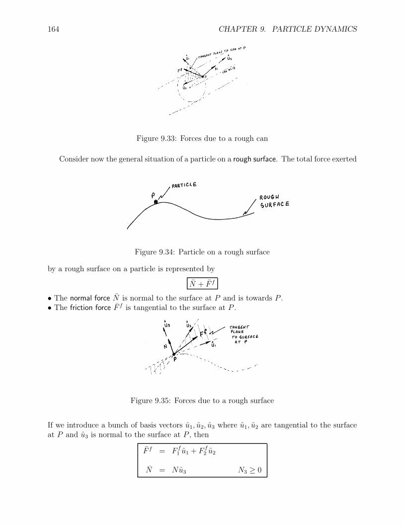
164 CHAPTER 9. PARTICLE DYNAMICS
Figure 9.33: Forces due to a rough can
Consider now the general situation of a particle on a rough surface. The total force exerted
Figure 9.34: Particle on a rough surface
by a rough surface on a particle is represented by
N + F f
• The normal force N is normal to the surface at P and is towards P .• The friction force F f is tangential to the surface at P .
Figure 9.35: Forces due to a rough surface
If we introduce a bunch of basis vectors u1, u2, u3 where u1, u2 are tangential to the surfaceat P and u3 is normal to the surface at P , then
F f = F f1 u1 + F f
2 u2
N = Nu3 N3 ≥ 0

9.10. ROUGH SURFACES, ROUGH CURVES AND FRICTION 165
Coulomb friction
A very common type of friction is Coulomb friction or dry friction. It usually occurs betweentwo dry solid bodies in contact with each other. How do we walk? Why do motorcyclesmove?
Consider the general situation of a particle which is constrained to remain on a roughsurface and suppose the friction force between the particle and the surface is due to Coulombfriction.
Figure 9.36: Particle moving relative to surface
The Coulomb friction force depends on whether there is relative motion between the particleand the surface. To describe this, introduce a reference frame e in which the surface is fixedand let v be the velocity of the particle in e, that is, v is the velocity of the particle relativeto the surface, that is relative to e.
Static friction. Consider first the case in which there is no motion of the particle relativeto the surface, that is, v = 0. Then the only additional statement that we can make aboutthe friction force F f exerted by the surface on the particle is that its magnitude F f mustsatisfy the inequality,
F f ≤ µN ,
where N = |N | is the magnitude of the normal force exerted by the surface on the particle.The nonnegative constant µ = µs is called a coefficient of static friction. It depends thesurface properties of the objects in contact. Some examples are:
rubber on asphalt: µs = 0.85
rubber on ice: µs = 0.1
In static friction, the friction force is determined by the other forces on the particle andby the acceleration of the particle. In general,
Ff =√
(F f1 )2 + (F f
2 )2
In one of the components is zero then the expression for F f is simpler, for example, if F f2 is
zero then,F f = |F f
1 | .

166 CHAPTER 9. PARTICLE DYNAMICS
Sliding friction. Consider now the case in which there is motion of the particle relative tothe surface, that is the particle is sliding on the surface and v 6= 0. In this case the directionof the friction force F f must be opposite to that of the velocity v. Also the magnitude F f
of the friction force must satisfy the equality
F f = µN
The non-negative constant µ = µk is called a coefficient of kinetic friction. It depends on thesurface properties of the objects in contact. Usually,
µk < µs
Why do you achieve maximum braking in a road vehicle by applying the brakes to thepoint where the wheels are just about to slip?

9.10. ROUGH SURFACES, ROUGH CURVES AND FRICTION 167
Example 45 Given: The block is in static equilibrium on the rough plane which is inclinedat an angle of θ to the horizontal. The coefficient of static friction between the block andthe plane is µ.
Figure 9.37: Example 45
Find: An expression for the maximum value of θ.Solution:

168 CHAPTER 9. PARTICLE DYNAMICS
Example 46 Given: The weight of the block is 9 lb and the coefficient of static frictionbetween the block and the rough surface is µ = 0.5.
Figure 9.38: Example 46
Find: out whether or not this block can be in static equilibrium?Solution:

9.10. ROUGH SURFACES, ROUGH CURVES AND FRICTION 169
Example 47 Given: The block is at rest relative to the rough inclined plane; this planerotates at a constant rate Ω about a vertical axis. The coefficient of static friction betweenthe block and the plane is µ. Consider γ = 45 and µ = 1/2.
Figure 9.39: Example 47
Find: Expressions for the range of possible values of Ω.Solution:

170 CHAPTER 9. PARTICLE DYNAMICS
Linear viscous friction
Sometimes, the friction between two lubricated bodies can be modelled as linear viscousfriction. This type of friction force is opposite in direction to the velocity v and is proportionalto v. Mathematicaly, this can be expressed as
F f = −cv
where the constant c is non-negative. This constant c is called a linear damping coefficient.Note that, unlike coulomb friction, this type of friction is zero when the velocity v is zero.
9.10.1 Rough curves
Similar to rough surfaces. Friction force is
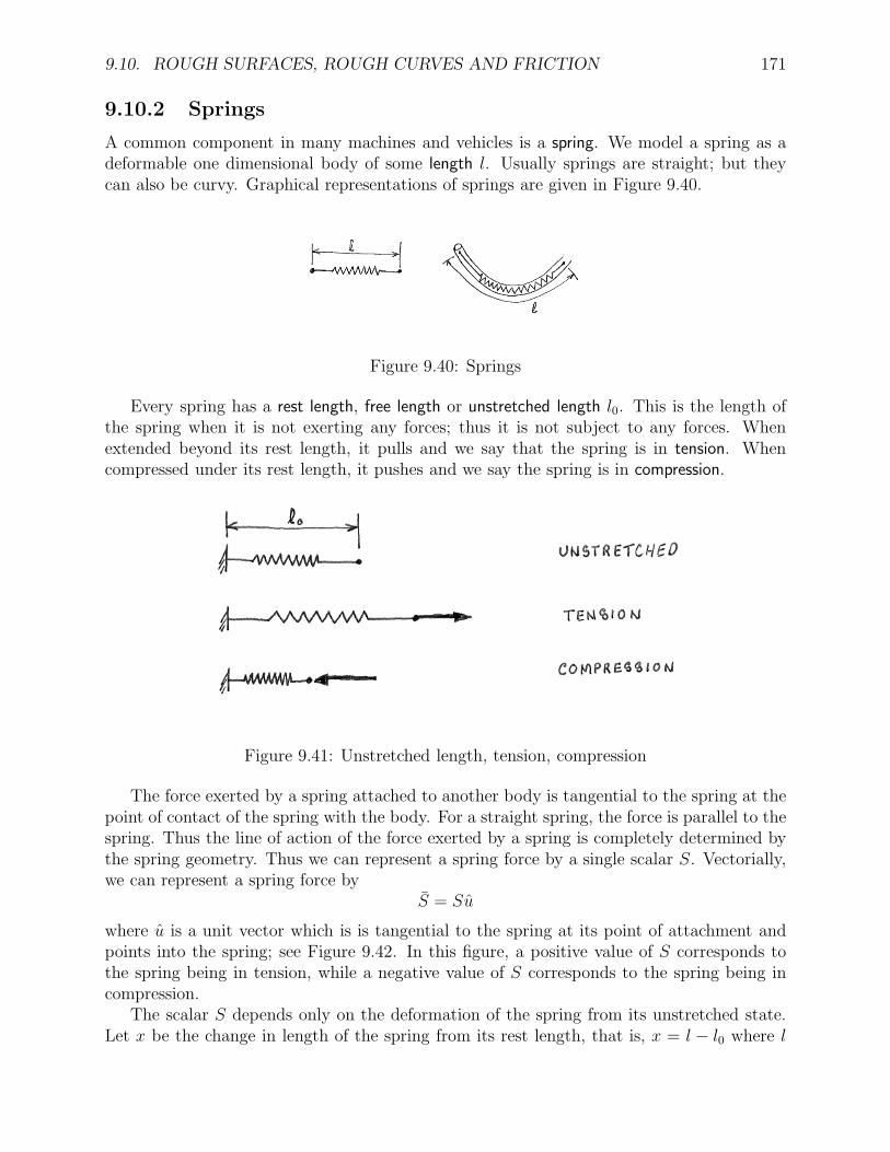
9.10. ROUGH SURFACES, ROUGH CURVES AND FRICTION 171
9.10.2 Springs
A common component in many machines and vehicles is a spring. We model a spring as adeformable one dimensional body of some length l. Usually springs are straight; but theycan also be curvy. Graphical representations of springs are given in Figure 9.40.
Figure 9.40: Springs
Every spring has a rest length, free length or unstretched length l0. This is the length ofthe spring when it is not exerting any forces; thus it is not subject to any forces. Whenextended beyond its rest length, it pulls and we say that the spring is in tension. Whencompressed under its rest length, it pushes and we say the spring is in compression.
Figure 9.41: Unstretched length, tension, compression
The force exerted by a spring attached to another body is tangential to the spring at thepoint of contact of the spring with the body. For a straight spring, the force is parallel to thespring. Thus the line of action of the force exerted by a spring is completely determined bythe spring geometry. Thus we can represent a spring force by a single scalar S. Vectorially,we can represent a spring force by
S = Su
where u is a unit vector which is is tangential to the spring at its point of attachment andpoints into the spring; see Figure 9.42. In this figure, a positive value of S corresponds tothe spring being in tension, while a negative value of S corresponds to the spring being incompression.
The scalar S depends only on the deformation of the spring from its unstretched state.Let x be the change in length of the spring from its rest length, that is, x = l − l0 where l

172 CHAPTER 9. PARTICLE DYNAMICS
Figure 9.42: Spring force
is the current length of the spring and l0 is the unstretched length of the spring. Then, xrepresents the amount by which the spring is extended (x > 0) or contracted (x < 0). AlsoS is positive when x is positive and S is negative when x is negative. The graph of S versus
Figure 9.43: Spring deflection
x for a spring is called the characteristic curve of the spring; see Figure 9.44.
Figure 9.44: Spring characteristic curve
The simplest characteristic characteristic curve is linear, that is,
S = kx
for some positive scalar k. This is sometimes referred to as Hookes Law and is illustrated inFigure 9.45. The proportionality constant k is called the spring constant for the spring. Ithas dimension FL−1 and possible units are N/m or lbs/ft.
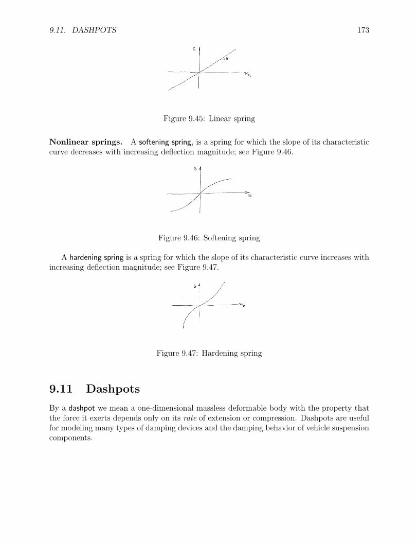
9.11. DASHPOTS 173
Figure 9.45: Linear spring
Nonlinear springs. A softening spring, is a spring for which the slope of its characteristiccurve decreases with increasing deflection magnitude; see Figure 9.46.
Figure 9.46: Softening spring
A hardening spring is a spring for which the slope of its characteristic curve increases withincreasing deflection magnitude; see Figure 9.47.
Figure 9.47: Hardening spring
9.11 Dashpots
By a dashpot we mean a one-dimensional massless deformable body with the property thatthe force it exerts depends only on its rate of extension or compression. Dashpots are usefulfor modeling many types of damping devices and the damping behavior of vehicle suspensioncomponents.
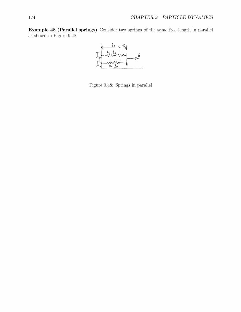
174 CHAPTER 9. PARTICLE DYNAMICS
Example 48 (Parallel springs) Consider two springs of the same free length in parallelas shown in Figure 9.48.
Figure 9.48: Springs in parallel

9.11. DASHPOTS 175
Example 49 (Series springs) Consider two springs in series as shown in Figure 9.48.
Figure 9.49: Springs in series

176 CHAPTER 9. PARTICLE DYNAMICS
Example 50 Given: W = 1 lb, k = 2 lb ft−1, µ = 1/2 and θ = 30.
Figure 9.50: Example 50
Find: The range of possible values of the spring deflection x.
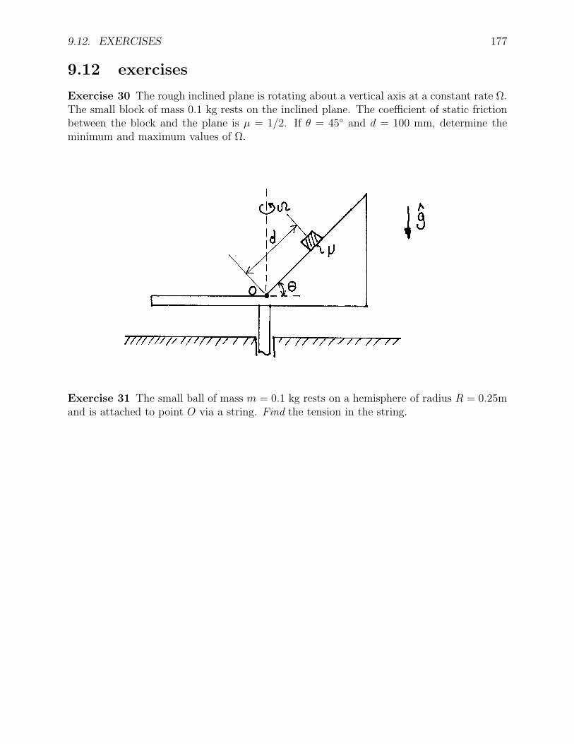
9.12. EXERCISES 177
9.12 exercises
Exercise 30 The rough inclined plane is rotating about a vertical axis at a constant rate Ω.The small block of mass 0.1 kg rests on the inclined plane. The coefficient of static frictionbetween the block and the plane is µ = 1/2. If θ = 45 and d = 100 mm, determine theminimum and maximum values of Ω.
Exercise 31 The small ball of mass m = 0.1 kg rests on a hemisphere of radius R = 0.25mand is attached to point O via a string. Find the tension in the string.

178 CHAPTER 9. PARTICLE DYNAMICS

Chapter 10
Equations of Motion
In designing a spacecraft or aircraft, we like to know how it is going to behave beforeflying it. If aircraft and pilots were expendable like darts, one could probably design themtotally by experimental trial and error, that is, dream up a design and fly the vehicle to see ifit is cool or sucks. Then based on the outcome, make modifications and “fly” again. This iscalled the Beavis and Butthead approach to aerospace vehicle design. Many men–women andmuch expense would have been incurred in trying to land on the moon by this method. So,before flying an aerospace vehicle, we want to be able to predict its behavior as accurately aspossible. This we do by developing a mathematical model of the vehicle. The most commonmodel is a set of differential equations which describe the motion of the vehicle. These arecalled equations of motion. Of course, the concept of an equation of motion applies to anysystem described by the laws of mechanics. Actually, the idea of describing the behavior of aphysical system using differential equation extends to all braches of engineering and science.It has even been used in economics. Let us begin with some simple systems.
10.1 Single degree of freedom systems
Example 1 (I’m falling) Consider particle P in vertical free fall near the surface of Y FHB.Neglecting any fluid resistance, application of ΣF = ma in a vertical direction yields
x = −g (10.1)
where g is the gravitational acceleration constant of YFHB. This equation is a second orderordinary differential equation. It has the property that, given any initial displacement x0
and any initial rate of displacement v0 at any initial time t0, it has a unique solution for x(t).Specifically, integrating (10.1) with respect to time over the interval [0, t] yields
x(t) − x(0) =∫ t
0−g dτ
hence,x(t) = v0 − gt
179
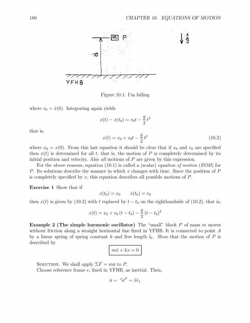
180 CHAPTER 10. EQUATIONS OF MOTION
Figure 10.1: I’m falling
where v0 = x(0). Integrating again yields
x(t) − x(t0) = v0t −g
2t2
that is,
x(t) = x0 + v0t −g
2t2 (10.2)
where x0 = x(0). From this last equation it should be clear that if x0 and v0 are specifiedthen x(t) is determined for all t, that is, the motion of P is completely determined by itsinitial position and velocity. Also all motions of P are given by this expression.
For the above reasons, equation (10.1) is called a (scalar) equation of motion (EOM) forP . Its solutions describe the manner in which x changes with time. Since the position of Pis completely specified by x, this equation describes all possible motions of P .
Exercise 1 Show that ifx(t0) = x0 x(t0) = v0
then x(t) is given by (10.2) with t replaced by t − t0 on the righthandside of (10.2), that is,
x(t) = x0 + v0 (t − t0) −g
2(t − t0)
2
Example 2 (The simple harmonic oscillator) The “small” block P of mass m moveswithout friction along a straight horizontal line fixed in YFHB. It is connected to point Aby a linear spring of spring constant k and free length l0. Show that the motion of P isdescribed by
mx + kx = 0
Solution. We shall apply ΣF = ma to P .Choose reference frame e, fixed in YFHB, as inertial. Then,
a = eaP = xe1

10.1. SINGLE DEGREE OF FREEDOM SYSTEMS 181
Figure 10.2: Simple harmonic oscillator
Figure 10.3: Kinematics of the simple harmonic oscillator
Application of ΣF = ma yields
−We2 + Ne2 − kx e1 = mx e1
The e1 components of the above equation yield:
e1 : −kx = mx
Hence,
mx + kx = 0 (10.3)
The above equation is an equation of motion for P . It is a linear, second order, ordinary,differential equation. It has the property that, given any initial displacement x0 and any
Figure 10.4: Free body diagram of P

182 CHAPTER 10. EQUATIONS OF MOTION
Figure 10.5: Simple harmonic oscillator with an attitude
initial rate of displacement v0 at some initial time t0, it has a unique solution for x(t) at anyother time t. In fact, with t0 = 0, the solution is given by:
x(t) = x0 cos(ωt) + (v0/ω) sin(ωt) (10.4)
where
x0= x(0) ; v0
= x(0) (10.5)
and
ω=√
k/m (10.6)
Note that we can rewrite (10.3) as
x + ω2x = 0 (10.7)
Exercise 2 Show that the above expression for x(t) is the solution to (10.3) with initialconditions (10.5).
Exercise 3 (Simple harmonic oscillator with an attitude) Show that the motion ofP is described by
mx + kx + g sin θ = 0
Example 3 (The simple pendulum) The simple pendulum consists of a particle P at-tached to a YFHB fixed point via a taut string of length l. It is constrained to move in avertical plane. The position of P is completely specified by θ, the angle between the stringand a vertical line. Show that the motion of P is governed by:
θ +g
lsin θ = 0
where g is the gravitational acceleration constant of YFHB.
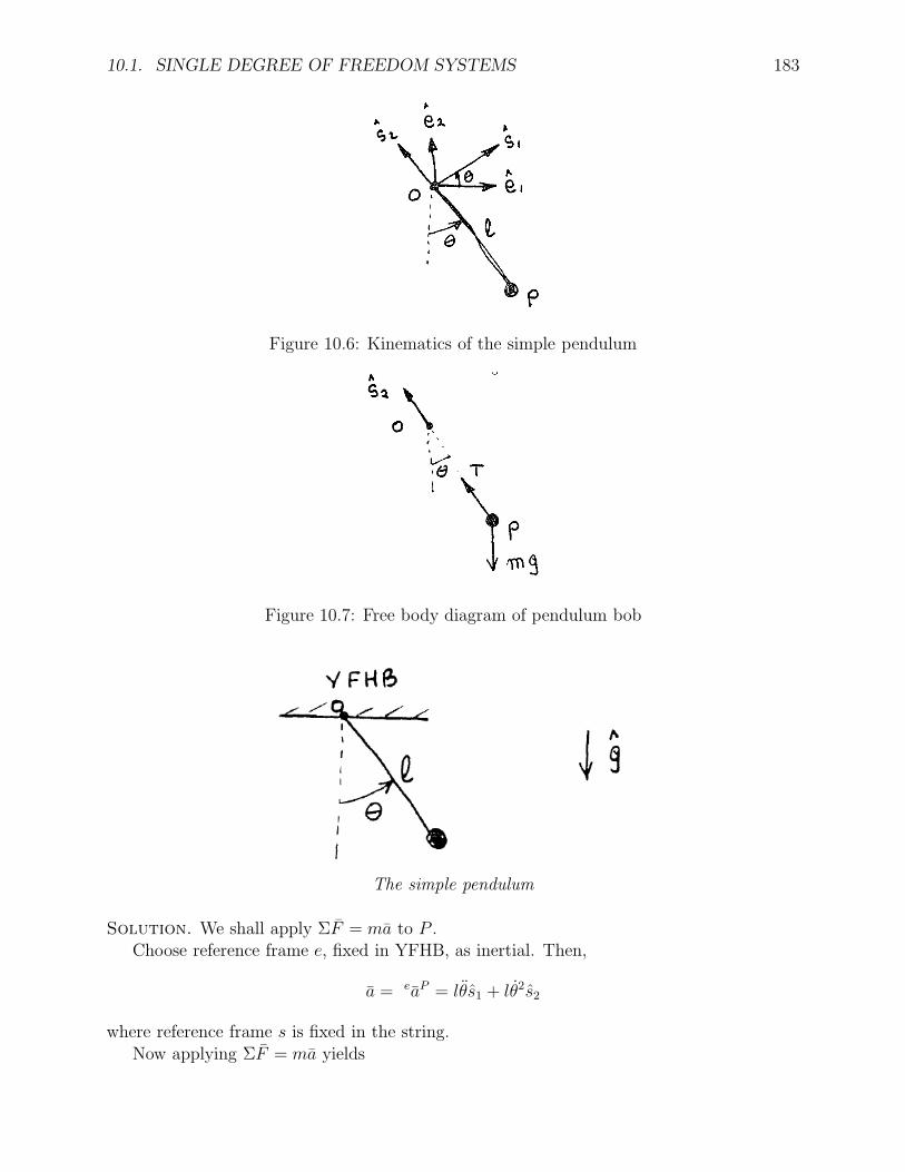
10.1. SINGLE DEGREE OF FREEDOM SYSTEMS 183
Figure 10.6: Kinematics of the simple pendulum
Figure 10.7: Free body diagram of pendulum bob
The simple pendulum
Solution. We shall apply ΣF = ma to P .Choose reference frame e, fixed in YFHB, as inertial. Then,
a = eaP = lθs1 + lθ2s2
where reference frame s is fixed in the string.Now applying ΣF = ma yields

184 CHAPTER 10. EQUATIONS OF MOTION
−mg e2 + T s2 = m(lθs1 + lθ2s2)
where m is the mass of P . Since
e2 = sin θ s1 + cos θ s2
we obtains1 : −mg sin θ = mlθ
s2 : −mg cos θ + T = mlθ2 (10.8)
The first equation yields
θ +g
lsin θ = 0 (10.9)
Note that application of ΣF = ma in the above example yielded two equations. Supposeyou were not given the EOM in the problem statement; why would you choose the first ofequations (10.8) as the EOM? In general an EOM should only depend on the coordinateof interest (θ in this case), its first and second derivatives, and system parameters such asmasses, spring constants, etc. Things like normal forces or string tensions should not appearin the final EOM. In the above example, one could use the second of the equations in (10.8)to solve for the string tension T as a function of P ’s motion. In general, if a particle isconstrained to move along a curve (a circle in this example) application of ΣF = ma in thethe direction tangential to the curve yields the equation of motion.
The above EOM is a second order nonlinear differential equation. It has the propertythat for each set of initial conditions:
θ(0) = θ0 θ(0) = θ0
there is a unique solution θ(t) satisfying these conditions. However, since the equation isnonlinear, you cannot use the techniques (Laplace etc.) learned in MA 262, MA 265, MA266 to solve it. Although it is possible to obtain exact solutions to this equation, in generalone cannot exactly solve nonlinear differential equations. To solve them one has to resolveto approximate numerical techniques .
A very special solution to (10.9) is the equilibrium solution
θ(t) ≡ 0
which corresponds to initial conditions θ(0) = θ(0) = 0. Suppose we are interested in thebehaviour of the system near this equilibrium solution. For “small” θ,
sin θ ≈ θ
10.2. NUMERICAL SIMULATION 185
and the EOM (10.9) can be approximated by
θ +g
lθ = 0 (10.10)
This looks familar, especially if we write it as
θ + ω2θ = 0
whereω =
√
g/l
(Recall (10.7)).All of the systems considered so far were described by a single second order differential
equation of the formF (x, x, x, t) = 0
This is because we only needed one coordinate to completely describe each of these systems.Such systems are called single degree of freedom systems. In a later section we look at multidegree of freedom systems.
10.2 Numerical simulation
10.2.1 First order representation
By appropriate definition of state variables
y1, y2, . . . , yn
one can rewrite any system of ordinary differential equations as a bunch of first order ordinarydifferential equations of the general form:
y1 = f1(t, y1, y2, . . . , yn)
y2 = f2(t, y1, y2, . . . , yn)...
yn = fn(t, y1, y2, . . . , yn)
Note that there is one equation for each state variable.
Example 51 The simple harmonic oscillator. Letting
y1 = x y2 := x
this system has the first order representation:
y1 = y2
y2 = − k
my1
186 CHAPTER 10. EQUATIONS OF MOTION
Example 52 The simple pendulum. With
y1 := θ y2 := θ
this system has the first order representation:
y1 = y2
y2 = −g
lsin y1

10.2. NUMERICAL SIMULATION 187
10.2.2 Numerical simulation with MATLAB
>> help ode45
ODE45 Solve differential equations, higher order method.
ODE45 integrates a system of ordinary differential equations using
4th and 5th order Runge-Kutta formulas.
[T,Y] = ODE45(’yprime’, T0, Tfinal, Y0) integrates the system of
ordinary differential equations described by the M-file YPRIME.M,
over the interval T0 to Tfinal, with initial conditions Y0.
[T, Y] = ODE45(F, T0, Tfinal, Y0, TOL, 1) uses tolerance TOL
and displays status while the integration proceeds.
INPUT:
F - String containing name of user-supplied problem description.
Call: yprime = fun(t,y) where F = ’fun’.
t - Time (scalar).
y - Solution column-vector.
yprime - Returned derivative column-vector; yprime(i) = dy(i)/dt.
t0 - Initial value of t.
tfinal- Final value of t.
y0 - Initial value column-vector.
tol - The desired accuracy. (Default: tol = 1.e-6).
trace - If nonzero, each step is printed. (Default: trace = 0).
OUTPUT:
T - Returned integration time points (column-vector).
Y - Returned solution, one solution column-vector per tout-value.
The result can be displayed by: plot(tout, yout).
See also ODE23, ODEDEMO.
Example 53 Lets say we want to numerically simulate the simple pendulum over the timeinterval 0 ≤ t ≤ 20 sec with parameters
l = 1 g = 1
and initial conditionsθ(0) = π/2 rad θ(0) = 0
We first write the equations in first order form; recall example 52. Next we create anM-file (lets call it pendulum.m) with the following lines.
function ydot = pendulum(t,y)
ydot(1) = y(2)
ydot(2) = -sin(y(1))

188 CHAPTER 10. EQUATIONS OF MOTION
We now simulate in MATLAB
>>[t,y]=ode45(’pendulum’,0,25,[pi/2; 0])
To get a plot:
>>plot(t,y)
0 2 4 6 8 10 12 14 16 18 20-2
-1.5
-1
-0.5
0
0.5
1
1.5
2
Now lets say we only want a plot of y1 vs t.
>>plot(t,y(:,1))
0 2 4 6 8 10 12 14 16 18 20-2
-1.5
-1
-0.5
0
0.5
1
1.5
2
Now suppose we want to plot y1 vs. y2. This is called a phase plane or state plane plot.
>>plot(y(:,1),y(:,2))

10.2. NUMERICAL SIMULATION 189
-2 -1.5 -1 -0.5 0 0.5 1 1.5 2-1.5
-1
-0.5
0
0.5
1
1.5

190 CHAPTER 10. EQUATIONS OF MOTION
10.3 Multi degree of freedom systems
Example 4 (The cannonball: ballistics in drag) Consider a cannonball P of mass min flight in a vertical plane near the surface of the earth. Suppose we model the aerodynamicforce on P as a force of magnitude D(v) acting opposite to the velocity v of the cannonballrelative to the earth and only dependent on the corresponding speed v := |v|. Show that themotion of P is governed by
p = v cos γ
h = v sin γmv = −mg sin γ − D(v)mvγ = −mg cos γ
(10.11)
where γ is the flight path angle and p and h are the horizontal range and altitude of P ,respectively
Figure 10.8: Cannonball
Solution. First note that
v =ed
dt(rOP )
=ed
dt(p e1 + h e2)
= pe1 + he2
Also,v = v cos γ e1 + v sin γ e2
Comparing these two expressions for v yields
p = v cos γ
h = v sin γ
Now we apply ΣF = ma to P .

10.3. MULTI DEGREE OF FREEDOM SYSTEMS 191
Reference frame u
Introduce reference frameu = (uv, uγ, u3)
where uv is the unit vector in the direction of v, uγ is the unit vector which is 90 degreescounterclockwise from uv, and u3 = e3. Then v = vuv;
eωu = γu3; and application of theBKE between frames u and e yields
a := eaP =ed
dt(v)
=ud
dt(v) + eωu × v
= v uv + vγ uγ
Free body diagram of P
Application of ΣF = ma yields:
uv : mv = −mg sin γ − D(v)uγ : mvγ = −mg cos γ
In the above example, the EOMs consisted of four first order differential equations. Wecould have obtained two second order differential equations in the coordinates p and h;however, they are not as nice as (10.11).

192 CHAPTER 10. EQUATIONS OF MOTION
Exercise 4 For the above example, obtain two second order differential equations whichdescribe the motion of P .
Exercise 5 (Sprung together) Consider a system consisting of two particles P1 and P2,connected together by a linear spring and constrained to move along a smooth horizontalline fixed in YFHB. Show that the motion of this system can be described by
m1q1 + k(q1 − q2) = 0m2q2 − k(q1 − q2) = 0
Sprung together
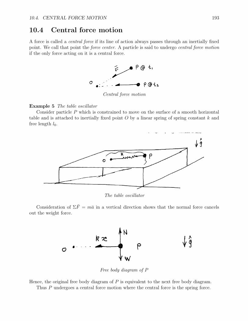
10.4. CENTRAL FORCE MOTION 193
10.4 Central force motion
A force is called a central force if its line of action always passes through an inertially fixedpoint. We call that point the force center. A particle is said to undergo central force motionif the only force acting on it is a central force.
Central force motion
Example 5 The table oscillatorConsider particle P which is constrained to move on the surface of a smooth horizontal
table and is attached to inertially fixed point O by a linear spring of spring constant k andfree length l0.
The table oscillator
Consideration of ΣF = ma in a vertical direction shows that the normal force cancelsout the weight force.
Free body diagram of P
Hence, the original free body diagram of P is equivalent to the next free body diagram.Thus P undergoes a central force motion where the central force is the spring force.
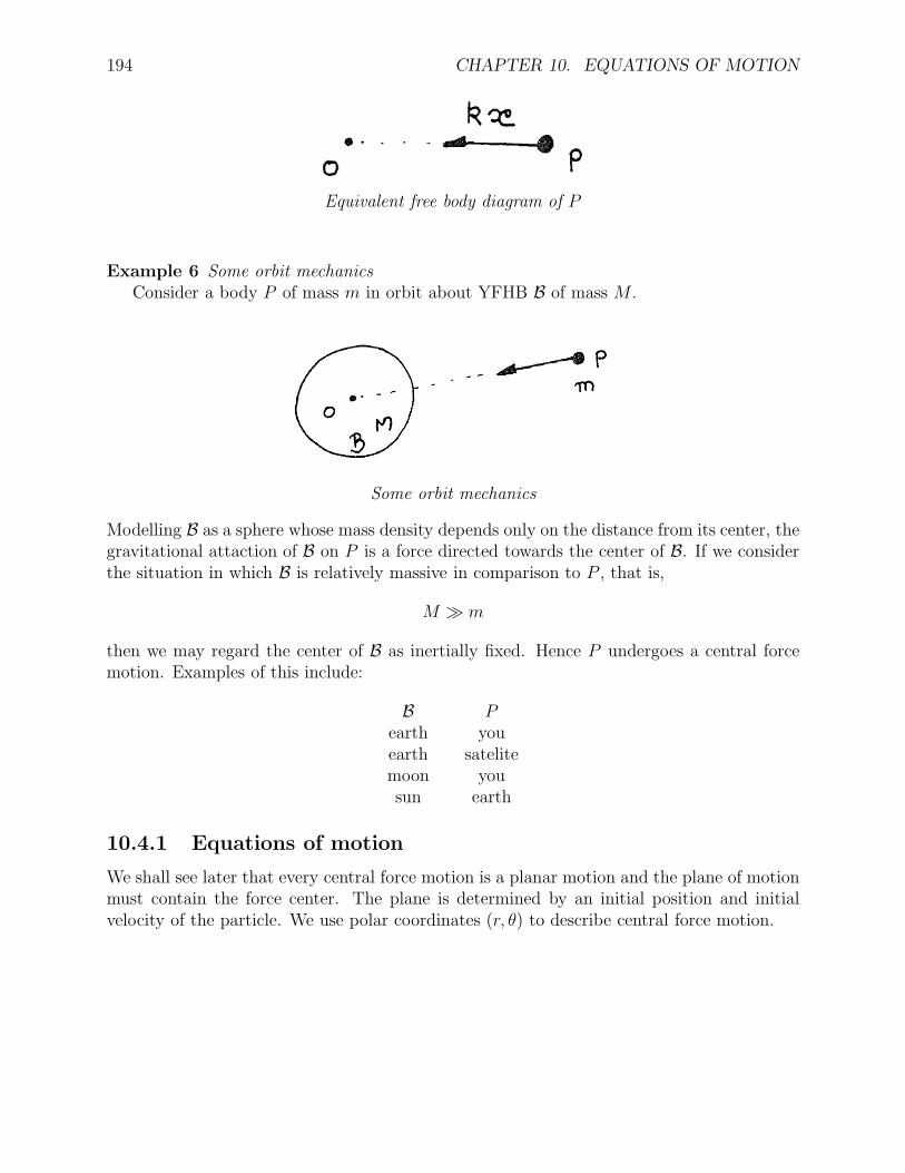
194 CHAPTER 10. EQUATIONS OF MOTION
Equivalent free body diagram of P
Example 6 Some orbit mechanicsConsider a body P of mass m in orbit about YFHB B of mass M .
Some orbit mechanics
Modelling B as a sphere whose mass density depends only on the distance from its center, thegravitational attaction of B on P is a force directed towards the center of B. If we considerthe situation in which B is relatively massive in comparison to P , that is,
M ≫ m
then we may regard the center of B as inertially fixed. Hence P undergoes a central forcemotion. Examples of this include:
B Pearth youearth satelitemoon yousun earth
10.4.1 Equations of motion
We shall see later that every central force motion is a planar motion and the plane of motionmust contain the force center. The plane is determined by an initial position and initialvelocity of the particle. We use polar coordinates (r, θ) to describe central force motion.

10.4. CENTRAL FORCE MOTION 195
Kinematics of central force motion
The inertial acceleration of P is given by
a = (r − rθ2) er + (rθ + 2rθ) eθ
Free body diagram of P
Applying ΣF = ma yields−F er = ma
Looking at the er and eθ components of ΣF = ma yields the following two EOMs:
r − rθ2 + F/m = 0
rθ + 2rθ = 0

196 CHAPTER 10. EQUATIONS OF MOTION
10.4.2 Some orbit mechanics
Consider the motion of a small body P of mass m about a much larger spherical body Bof mass M . We can regard the center of the spherical body as inertially fixed; hence themotion of the smaller body is a central force motion with
F =GMm
r2
Some orbit mechanics
Recalling the above EOMs for general central force motion, the motion of P is describedby
r − rθ2 + µ/r2 = 0
rθ + 2rθ = 0
where µ := GM .All solutions of the above two differential equations are conic sections; that is they satisfy
an equation of the form:
r =a
1 + b cos(θ − c)
The constants a, b, and c depend on the motion.
b = 0 circle0 < b < 1 ellipse
b = 1 parabolab > 1 hyperbola
For the moment, we will only look at circular orbits. AAE 340 contains a closer look atall orbits. AAE 532 (Orbit mechanics) is a whole course devoted to orbit mechanics.
Circular orbits
Let’s look for solutions corresponding to circular orbits, that is,
r(t) ≡ R
where R is constant; hence r = r = 0. The above EOMs reduce to
−Rθ2 + µ/R2 = 0
Rθ = 0

10.4. CENTRAL FORCE MOTION 197
The second equation implies that θ is constant, that is,
θ(t) ≡ ω
where ω is constant. The first equation now implies that
R3ω2 = µ
henceω =
√
µ/R3 or R = (µ/ω2)1/3 (10.12)
Geostationary orbits
Suppose one wants to position a satellite so that it always remains above a fixed point onthe earth. To study this motion, we need to take an inertial reference frame in which theearth rotates about its north-south axis at the rate:
ωe = 1rev/24 hour
=(2πrad)
(24)(60)(60) sec
= 7.272 × 10⁻⁵ rad/sec
Inertial reference frame
Since the satellite must move in a plane which contains the center of the earth, it mustbe located above the equator.
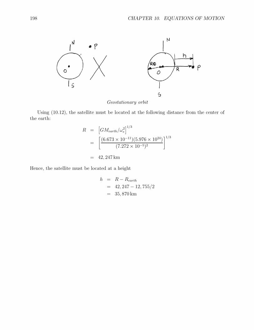
198 CHAPTER 10. EQUATIONS OF MOTION
Geostationary orbit
Using (10.12), the satellite must be located at the following distance from the center ofthe earth:
R =[
GMearth/ω2e
]1/3
=
[
(6.673 × 10⁻¹¹)(5.976 × 1024)
(7.272 × 10⁻⁵)2
]1/3
= 42, 247 km
Hence, the satellite must be located at a height
h = R − Rearth
= 42, 247 − 12, 755/2
= 35, 870 km

Chapter 11
Statics of Bodies
Prior to this, we have considered the statics of particles. In this chapter, we consider thestatics of general bodies. First, we need a new concept which is basic in the study of thestatics and dynamics of bodies, namely, the moment of a force.
11.1 The moment of a force
The moment of a force about a point is its turning effect about that point. As an example,think of a person pushing or pulling on one end of a joystick and consider the turning effectof this force about the pivot point at the other end of the joystick. The formal definition ofa moment is as follows.
The moment of a force F about a point Q is defined by
MQ = r × F
where r = QP (the vector from Q to P ) and P is the point of application of F .
•
• P
Q
r
F
Figure 11.1: Moment of a force
• Recalling the definition of the cross product, it follows that
MQ = MQ n where MQ = rF sin θ
199

200 CHAPTER 11. STATICS OF BODIES
Here r is the distance from Q to the point of application of the force, F is the magnitude ofthe force, θ is the angle between r and F , and n is the unit vector which is normal to bothr and F and whose sense is given by the right-hand rule; see Figure 11.2. Note that MQ isthe magnitude of MQ.
•
•
Q
r
F θ
n
Figure 11.2: Moment of a force again
• Units: newton-meter (N·m) or foot-pound (ft·lb).

11.1. THE MOMENT OF A FORCE 201
Example 54

202 CHAPTER 11. STATICS OF BODIES
The next fact tells us that in evaluating the moment of a force, we can choose the positionvector to terminate at any point on the line of action of the force.
Fact 2 If P is any point on the line of action of F , then
MQ = r × F
where r = QP (the vector from Q to P ).
Figure 11.3: Any point on the line of action will do.
Proof. By definition,MQ = QP ∗ × F
where P ∗ is the point of application of F . Since
QP ∗ = QP + PP ∗
we haveMQ = QP × F + PP ∗ × F
Since the points P and P ∗ are on the line of action of F , the vector PP ∗ is along the line ofaction of F ; hence
PP ∗ × F = 0
andMQ = QP × F

11.1. THE MOMENT OF A FORCE 203
Example 55

204 CHAPTER 11. STATICS OF BODIES
The following fact is useful for determining moments by inspection, especially in planarproblems.
Fact 3 If d is the distance from a point Q to the line of action of a force of magnitude F,then the magnitude MQ of the moment of that force about Q is given by
MQ = dF .
Figure 11.4: MQ = dF
Proof. Let P be the point on the line of action of F which is closest to Q. Thenthe vector QP is perpendicular to F and the magnitude of this vector is d. Using the firstdefinition of the cross product, we have
MQ = |MQ| = |QP × F |= |QP ||F | sin(90)
= dF
Note that the direction of the moment is determined by the right-hand rule. The next resultis an immediate consequence of the previous fact.
Fact 4 Suppose F is a nonzero force. Then its moment about a point Q is zero if and onlyif Q is on the line of action of F .

11.1. THE MOMENT OF A FORCE 205
Example 56
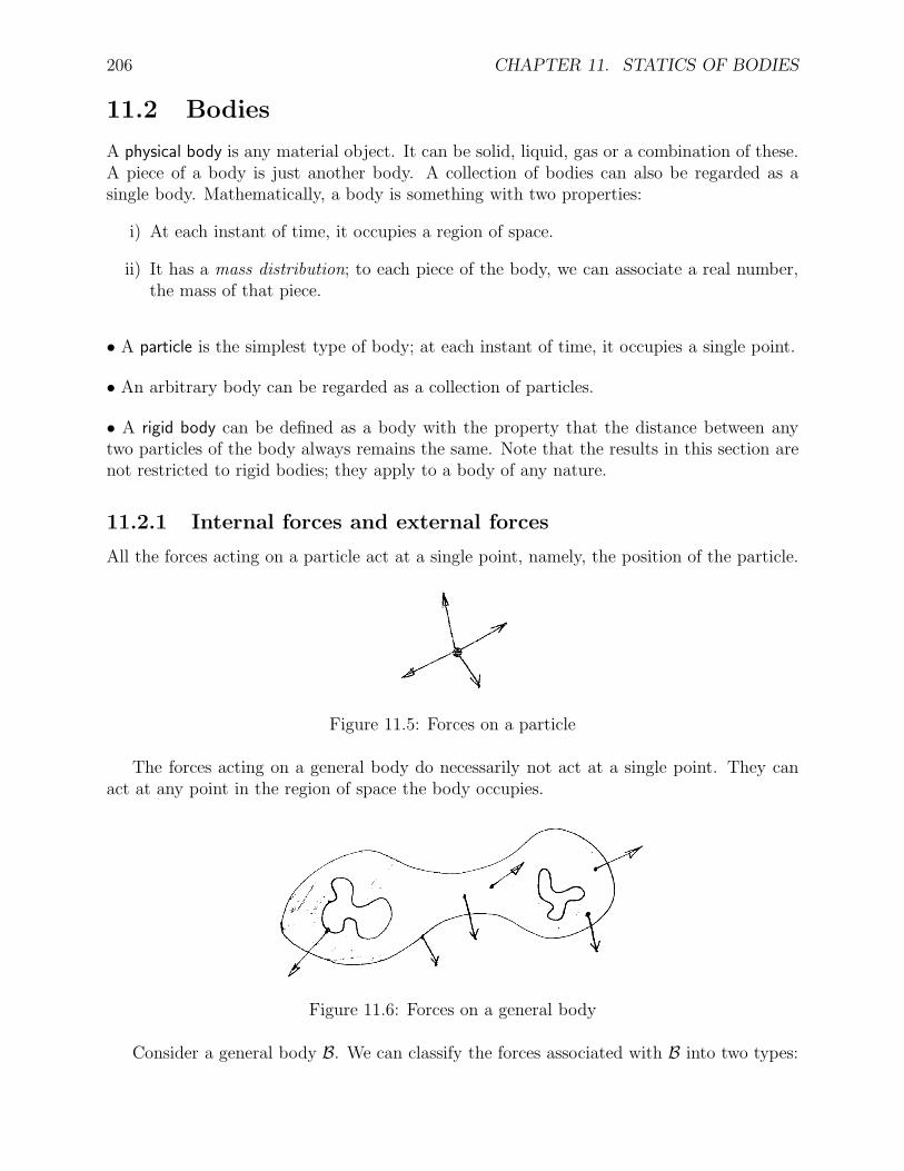
206 CHAPTER 11. STATICS OF BODIES
11.2 Bodies
A physical body is any material object. It can be solid, liquid, gas or a combination of these.A piece of a body is just another body. A collection of bodies can also be regarded as asingle body. Mathematically, a body is something with two properties:
i) At each instant of time, it occupies a region of space.
ii) It has a mass distribution; to each piece of the body, we can associate a real number,the mass of that piece.
• A particle is the simplest type of body; at each instant of time, it occupies a single point.
• An arbitrary body can be regarded as a collection of particles.
• A rigid body can be defined as a body with the property that the distance between anytwo particles of the body always remains the same. Note that the results in this section arenot restricted to rigid bodies; they apply to a body of any nature.
11.2.1 Internal forces and external forces
All the forces acting on a particle act at a single point, namely, the position of the particle.
Figure 11.5: Forces on a particle
The forces acting on a general body do necessarily not act at a single point. They canact at any point in the region of space the body occupies.
Figure 11.6: Forces on a general body
Consider a general body B. We can classify the forces associated with B into two types:

11.2. BODIES 207
• Forces internal to the body B. An internal force is a force exerted by one piece of Bon another piece of B.
• Forces external to the the body B. These are the forces exerted on B by other bodies.
11.2.2 Internal forces
By considering a body as a collection of particles and applying Newton’s third law, one canobtain the following result.
Theorem 2 (Internal forces) The internal forces of any body satisfy
∑int F = 0
∑int MQ = 0
for every point Q where
∑int F is the sum of all the internal forces in the body, and
∑int MQ is the sum of the moments about Q of all the internal forces in the body
Proof. Consider a general body B which we will regard as a collection of N particlesP1, P2, . . . , PN .
Let F jk be the resultant internal force exerted on particle Pj by particle Pk.

208 CHAPTER 11. STATICS OF BODIES
Thus the internal force system of B consists of the forces
F jk, j 6= k, j, k = 1, 2, . . . , N
First note that the resultant of all the internal forces is given by
int∑
F =N∑
j=1
N∑
k = 1k 6= j
F jk
= 0 + F 12 + F 13 + . . . + F 1N
+ F 21 + 0 + F 23 + . . . + F 2N
+ F 31 + F 32 + 0 + . . . + F 3N
......
......
+ F N1 + F N2 + F N3 + . . . + 0
= (F 12 + F 21) + (F 13 + F 31) + . . . + (F 1N + F N1)
+ (F 23 + F 32) + . . . + (F 2N + F N2)
+ (F 3N + F N3)...
+ 0
=N−1∑
j=1
N∑
k=j+1
(F jk + F kj)
By the first part of Newton’s Third Law, F kj = −F jk;
henceF jk + F kj = 0

11.2. BODIES 209
Thus,∑int F = 0
Consider now any corresponding pair of internal forces F jk, F kj. By the second part ofNewtons Third Law the line of action of these two forces must be the line joining Pj and Pk;hence the vector PkPj is parallel to F jk and F kj.
So,PkPj × F jk = 0
Evaluating the sum of the moments of these two forces about any point Q and using F kj =−F jk we get
rj × F jk + rk × F kj = (rj − rk) × F jk
= PkPj × F jk
= 0
Hence, the moments due to the internal forces cancel out in pairs. If∑int MQ is the sum of
the moments of all the internal forces about Q, then using the same computations we usedfor
∑int F we must have∑int MQ = 0
• Note that the above result holds regardless of the motion of the body; the body does nothave to be in static equilibrium (see next section).
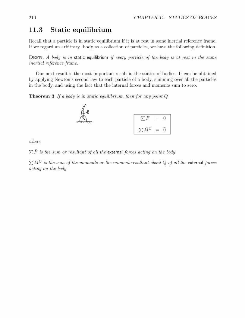
210 CHAPTER 11. STATICS OF BODIES
11.3 Static equilibrium
Recall that a particle is in static equilibrium if it is at rest in some inertial reference frame.If we regard an arbitrary body as a collection of particles, we have the following definition.
DEFN. A body is in static equilibrium if every particle of the body is at rest in the sameinertial reference frame.
Our next result is the most important result in the statics of bodies. It can be obtainedby applying Newton’s second law to each particle of a body, summing over all the particlesin the body, and using the fact that the internal forces and moments sum to zero.
Theorem 3 If a body is in static equilibrium, then for any point Q
∑
F = 0
∑
MQ = 0
where
∑
F is the sum or resultant of all the external forces acting on the body
∑
MQ is the sum of the moments or the moment resultant about Q of all the external forcesacting on the body
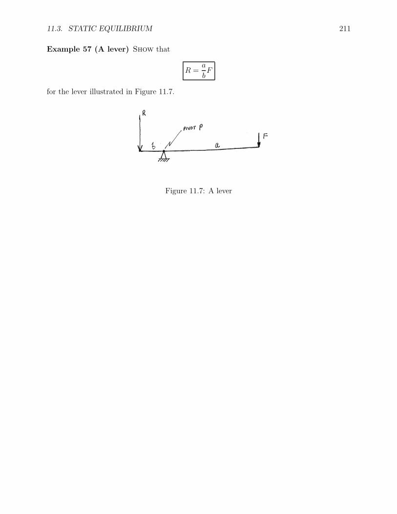
11.3. STATIC EQUILIBRIUM 211
Example 57 (A lever) Show that
R =a
bF
for the lever illustrated in Figure 11.7.
Figure 11.7: A lever

212 CHAPTER 11. STATICS OF BODIES
Example 58 (Another lever) Show that
R =a
bF
for the lever illustrated in Figure 11.8.
Figure 11.8: Another lever

11.3. STATIC EQUILIBRIUM 213
Example 59 (Yet another lever) Show that
R =a
bF
for the lever illustrated in Figure 59.
Figure 11.9: Yet another lever

214 CHAPTER 11. STATICS OF BODIES
11.3.1 Free body diagrams
Body + External forces
Examples of FBDs
Example 60
Figure 11.10: Example 60

11.3. STATIC EQUILIBRIUM 215
Example 61
Figure 11.11: Example 61

216 CHAPTER 11. STATICS OF BODIES
Example 62
Figure 11.12: Example 62

11.4. EXAMPLES IN STATIC EQUILIBRIUM 217
11.4 Examples in static equilibrium
11.4.1 Scalar equations of equilibrium
In general, the two vector equations
ΣF = 0
ΣMQ = 0
yield six scalar equations. However, in some cases, the six equations are not independent orsome are trivial, for example, 0 = 0. The following are force systems which do not give riseto six independent scalar equations of equilibrium.
Force system Max. no. of independent scalar equationscollinear 1coplanar 3parallel 3parallel to a common plane 5
11.4.2 Planar examples
A planar problem is one in which all the bodies and forces of interest lie in a single plane.Suppose e1, e2, e3 is an orthogonal triad of unit vectors with e1, e2 lying in the plane ofinterest and with e3 perpendicular to the plane. Then all forces and position vectors can beexpressed in terms of e1 and e2; hence all moments are parallel to e3. So, the conditions ofstatic equilibrium give rise to at most three nontrivial scalar equations:
e1 :∑
F1 = 0e2 :
∑
F2 = 0e3 :
∑
MQ = 0

218 CHAPTER 11. STATICS OF BODIES
Example 63 Given: The block of weight W = 10 lb sits on the massless beam which issupported at A and B by frictionless roller supports.
Figure 11.13: Example 63
Find: the reactions on the beam at A and B.

11.4. EXAMPLES IN STATIC EQUILIBRIUM 219
Example 64 Given: The block of weight W = 100 N sits on a massless bar which issupported at A and B by cables.
Figure 11.14: Example 64
Find: the tension in each cable at the bar.

220 CHAPTER 11. STATICS OF BODIES
Example 65 Given: The Lunacycle of weight W is parked on a hill which is inclined at anangle of θ to the horizontal.
Figure 11.15: Example 65
Find: expressions for the magnitude of normal force on each wheel.
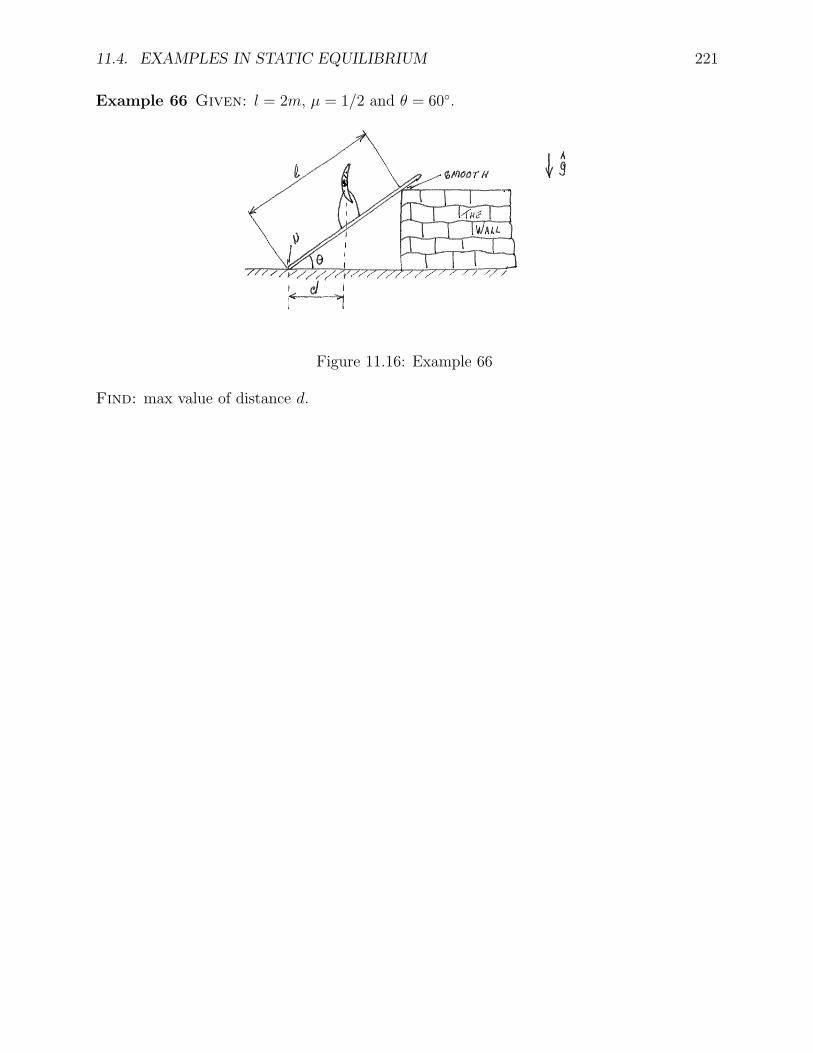
11.4. EXAMPLES IN STATIC EQUILIBRIUM 221
Example 66 Given: l = 2m, µ = 1/2 and θ = 60.
Figure 11.16: Example 66
Find: max value of distance d.

222 CHAPTER 11. STATICS OF BODIES
Example 67 Given: A uniform stepped cylinder with radii R = 1m, r = 0.5m and weightW = 100N is in static equilibrium on a rough horizontal plane and is attached to two cablesat points A and B. Also, µ = 1/4.
Figure 11.17: Example 63
Find: the maximum value of the cable tension T .

11.4. EXAMPLES IN STATIC EQUILIBRIUM 223
11.4.3 General examples
Example 68 Given: The block of weight W = 20 lb is resting on the massless plate whichis supported at A, B and C by cables.
Figure 11.18: Example 63
Find: the tensions in the cables at points A, B and C.

224 CHAPTER 11. STATICS OF BODIES
11.5 Force systems
Here we develop some general properties of force systems. A force system is just a bunch offorces, F 1 , F 1 , . . . , F N as illustrated in Figure 11.19
Figure 11.19: A force system
DEFN. The resultant of a force system is the sum of all its forces and is given by:
∑
F :=N∑
j=1
F j = F 1 + F 2 + . . . + F N
DEFN. The moment resultant of a force system about a point Q is the sum of the momentsof all its forces about Q and is given by:
∑
MQ :=N∑
j=1
rj × F j = r1 × F 1 + r2 × F 2 + . . . + rN × F N
where rj is a vector from Q to a point on the line of action of F j.
Figure 11.20: Moment resultant
Suppose one knows the resultant and moment resultant about some point Q′ of a forcesystem. The following result tells us how to compute the moment resultant about anotherpoint Q without having to compute all the moments of all the forces about Q.
Fact 5 For any two points Q and Q′
,
∑
MQ =∑
MQ′
+ r × ΣF
where r = rQQ′
(the vector from Q to Q′
).
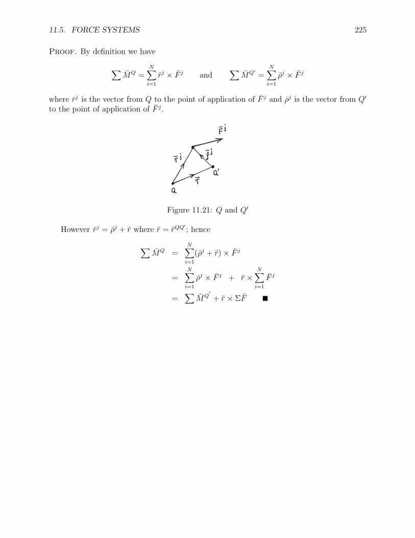
11.5. FORCE SYSTEMS 225
Proof. By definition we have
∑
MQ =N∑
i=1
rj × F j and∑
MQ′
=N∑
i=1
ρj × F j
where rj is the vector from Q to the point of application of F j and ρj is the vector from Q′
to the point of application of F j.
Figure 11.21: Q and Q′
However rj = ρj + r where r = rQQ′
; hence
∑
MQ =N∑
i=1
(ρj + r) × F j
=N∑
i=1
ρj × F j + r ×N∑
i=1
F j
=∑
MQ′
+ r × ΣF

226 CHAPTER 11. STATICS OF BODIES
Example 69 Here we illustrate the moment formula just developed. Consider the forcesystem in Figure 11.22.
Figure 11.22: Force system for Example 69

11.5. FORCE SYSTEMS 227
11.5.1 Couples and torques
DEFN. A couple is a pair of forces which have equal magnitude but opposite direction.
Figure 11.23: A couple
So, if (F 1, F 2) is a couple, then,
F 2 = −F 1 .
• A couple has zero resultant.• The moment resultant of a couple about every point is the same.
DEFN. The torque T of a couple is its moment resultant about any point.
Quite often, we are only interested in the torque of a couple and we are not necessarilyinterested in the two forces that make up the couple. So, we often represent a couple by itstorque T . In graphic representations of torque vectors, we use a double arrowhead insteadof the usual single arrowhead.
Figure 11.24: Representations of torque

228 CHAPTER 11. STATICS OF BODIES
Example 70 Each of the following couples are equivalent.

11.6. EQUIVALENT FORCE SYSTEMS 229
11.6 Equivalent force systems
DEFN. Two force systems are equivalent if they have the same resultant and the same momentresultant about some point.
So, the system of internal forces in any body is equivalent to a zero force. Also, if a bodyis in static equilibrium, its system of external forces is equivalent to a zero force.
Example 71 Consider the following force system.
2 m
2 N
3N
It is equivalent to any of the following force systems.
5 N
6 N m5 N
4 N m
5 N
6/5 m 4/5 m

230 CHAPTER 11. STATICS OF BODIES
• If two force systems are equivalent, then they have the same moment about every point.
This follows from the relationship,∑
MQ =∑
MQ′
+ r × ΣF .
You will see later that if two force systems are equivalent, then they have exactly thesame effect when applied to a given rigid body.
11.7 Simple equivalent force systems
Sometimes it is very useful to replace a complicated force system by a simpler equivalentforce system.
11.7.1 A force and a couple
Every force system (regardless of complexity) is equivalent to a force and a couple. To seethis, choose any point Q and let
F = ΣF and T = ΣMQ
It can readily seen that the new force system consisting of a force F placed at Q and a coupleof torque T is equivalent to the original force system.
Note that Q can be any point.
11.7.2 Force systems which are equivalent to a couple
Suppose that a force has zero resultant, that is,
ΣF = 0
Then this force system is equivalent to a couple of torque T = ΣMQ. Since ΣF = 0, thistorque is independent of the point Q.

11.7. SIMPLE EQUIVALENT FORCE SYSTEMS 231
Example 72
Figure 11.25: A force system which is equivalent to a couple

232 CHAPTER 11. STATICS OF BODIES
11.7.3 Force systems which are equivalent to single force
Suppose there is a point Q about which the force system has zero moment resultant, that is,
ΣMQ = 0
Then this force system is equivalent to a single force F = ΣF whose point of application isQ.
Example 73
Figure 11.26: A force system which is equivalent to a single force
The single force

11.7. SIMPLE EQUIVALENT FORCE SYSTEMS 233
Note that the point of application of a single equivalent force is not unique. One can“slide” a single equivalent force along its line of application and obtain another equivalentforce with a different point of application.
We now demonstrate the following result.
A force system is equivalent to a single force if and only if it has non-zero resultant andthe moment resultant about some point is perpendicular to the resultant.
Suppose one has a force system which is equivalent to single force F placed at a pointQ. Let T =
∑
MO where O is any point. Then it is necessary that T is perpendicular to F .This can be seen as follows. Since F placed at Q is equivalent to the original force system,the moment of F about O must equal the moment resultant of the original force systemabout O, that is,
r × F = T (11.1)
where r is the vector from O to Q. The above expression and the properties tell that T isperpendicular to F .
Now suppose we know that F and T are perpendicular with F 6= 0. We claim that onecan always find a vector r such that (11.1) holds. One such vector is given by
r =F × T
F 2. (11.2)
where F is the magnitude of F . This can be seen as follows. Recall that for any three vectorsU , V and W we have
U × (V × W ) = (U · W )V − (U · V )W .
Hence
r × F =
(
F × T
F 2
)
× F = − 1
F 2
(
F × (F × T ))
= − 1
F 2
(
(F · T )F − (F · F )T)
.
Since, by assumption, F is perpendicular to T we must have F · T = 0. Also, F · F = F 2.Hence, we obtain that r × F = T .
The following force systems are examples of force systems which are equivalent to a singleforce.
Concurrent force system
Here the line of each force passes through a common point.

234 CHAPTER 11. STATICS OF BODIES
Planar force systems with non-zero resultant
Example 74
Figure 11.27: A planar force system which is equivalent to a single force

11.7. SIMPLE EQUIVALENT FORCE SYSTEMS 235
Parallel force systems with non-zero resultant*
Example 75
Figure 11.28: A parallel force system which is equivalent to a single force

236 CHAPTER 11. STATICS OF BODIES
Parallel force systems. Choose a reference frame so that all the forces are parallel to e3.Then every force F j can be expressed as
F j = F j e3
and
ΣF = F e3 where F :=N∑
i=1
F j
Let O be the origin of the reference frame and let rj be the vector from O to the point ofapplication of F j; then rj can be expressed as
rj = xj e1 + yj e2 + zj e3
Hence,rj × F j = (yjF j) e1 − (xjF j) e2
and
ΣMO = T1 e1 + T2 e2 where T1 :=N∑
i=1
yjF j and T2 := −N∑
i=1
xjF j .
Lettingr∗ = x∗ e1 + y∗ e2 + z∗ e3
be the vector from O to the point of application of F we get
r∗ × F = (y∗N∑
i=1
F j) e1 − (x∗N∑
i=1
F j) e2
Since r∗ × F = ΣMO, we obtain
y∗N∑
i=1
F j =N∑
i=1
yjF j
x∗N∑
i=1
F j =N∑
i=1
xjF j
Hence
x∗ =∑N
i=1xjF j
F
y∗ =∑N
i=1yjF j
F

11.8. DISTRIBUTED FORCE SYSTEMS 237
11.8 Distributed force systems
So far, we have considered forces to act at a single point. Here we look at forces which donot act a single point, but act over a region of space. We divide these forces into body forcesand surface forces.
11.8.1 Body forces
A body force acts over a three-dimensional region of space. The main example of a bodyforce is the gravitational attraction of one body on another.
Gravitational forces
The gravitational force exerted by one body (the offending body) on another body (thesuffering body) is a force system which is distributed throughout the entire suffering body.Every particle of the suffering body is subject to the gravitational attraction of the offendingbody. When the offending body is YFHB and the suffering body is near the surface ofYFHB and its dimensions are insignificant compared to YFHB then, all the gravitationalforce system is in the same direction, namely, in the direction of the local vertical g. Sothis gravitational force system is a parallel force system. It is equivalent to a single force Wplaced at the mass center of the suffering body and given by
W = Wg
where W is called the weight of the suffering body and is given by
W = mg
where m is the mass of the suffering body and g is the gravitational acceleration constant ofYFHB. For bodies of uniform mass density, the mass center is at the geometric center. Notethat the mass center does not have to be a point on the body; see donut.
Figure 11.29: Weight
When the suffering body is not near the surface of YFHB (think of a spacecraft in orbitaround the earth) then, the gravitational forces on the suffering body may have a non-zeromoment resultant about the mass center of the suffering body.

238 CHAPTER 11. STATICS OF BODIES
Figure 11.30: Some mass centers
11.8.2 Surface forces
A surface force acts over a two-dimensional region of space. One example of a surface force ishydrostatic force, that is, the forces exerted on a body when it is immersed in water. Anotherexample is aerodynamic forces, that is the forces on a body moving relative to the air.
Hydrostatic forces
Archimedes principle, center of buoyancy

11.8. DISTRIBUTED FORCE SYSTEMS 239
Aerodynamic forces
If you pick any reference point on an aircraft, the aerodynamic force system is equivalent toa single force F placed at the point and a moment T . F is independent of the point whereasT is the moment resultant of the force about that point; hence it depends on the point. If Tis zero, that point is called a center of pressure. In general the center of pressure changes asthe aircraft changes its orientation relative to the wind; it is not a fixed point on the aircraft.There is usually another point which is fixed and has the property that T is constant forthat point; this is the aerodynamic center.lift, drag, pitching moment,
Figure 11.31: Aerodynamic forces
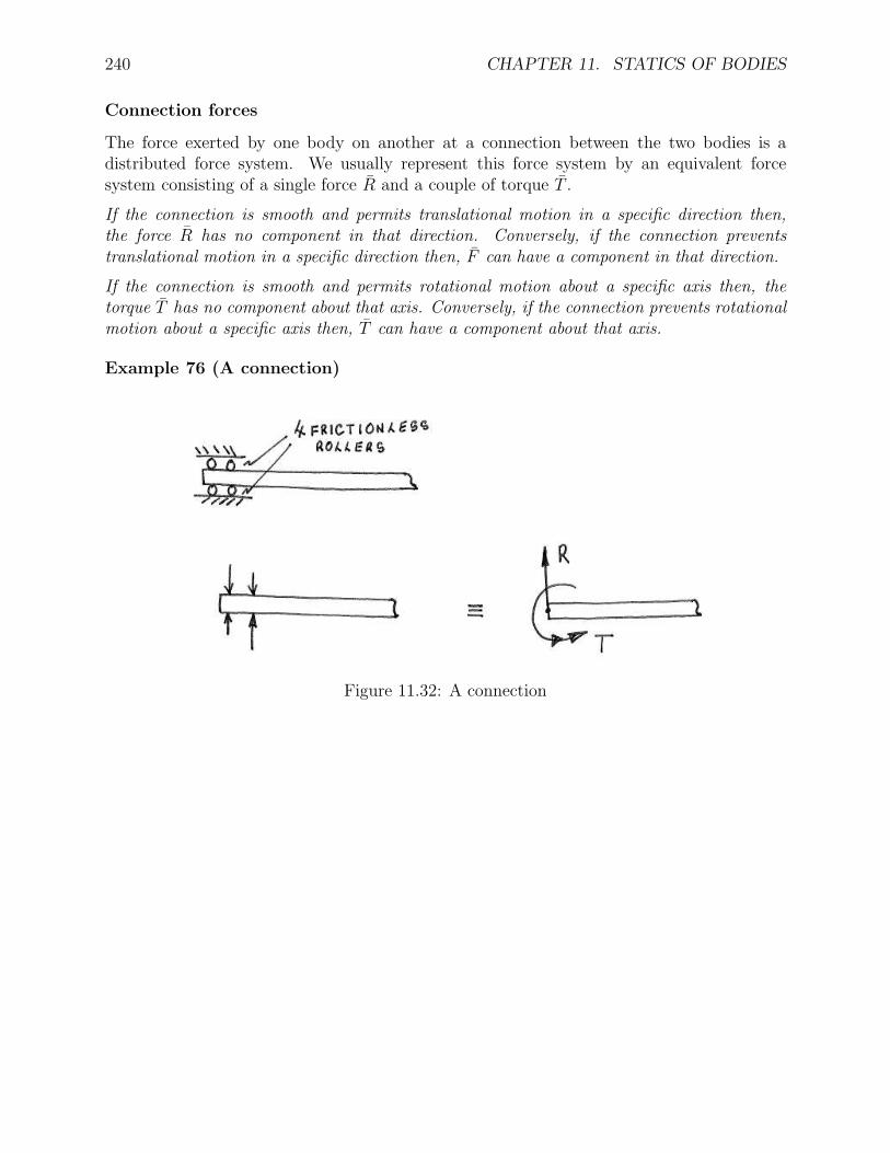
240 CHAPTER 11. STATICS OF BODIES
Connection forces
The force exerted by one body on another at a connection between the two bodies is adistributed force system. We usually represent this force system by an equivalent forcesystem consisting of a single force R and a couple of torque T .
If the connection is smooth and permits translational motion in a specific direction then,the force R has no component in that direction. Conversely, if the connection preventstranslational motion in a specific direction then, F can have a component in that direction.
If the connection is smooth and permits rotational motion about a specific axis then, thetorque T has no component about that axis. Conversely, if the connection prevents rotationalmotion about a specific axis then, T can have a component about that axis.
Example 76 (A connection)
Figure 11.32: A connection

11.8. DISTRIBUTED FORCE SYSTEMS 241
Example 77 (Another connection)
Figure 11.33: Another connection

242 CHAPTER 11. STATICS OF BODIES
11.8.3 Connections in 2D
We are assuming no friction at these connections.
Figure 11.34: Frictionless connections in 2D

11.8. DISTRIBUTED FORCE SYSTEMS 243
11.8.4 Connections in 3D

244 CHAPTER 11. STATICS OF BODIES
11.9 More examples in static equilibrium
Example 78 Given: The load of weight W = 100N is supported by the massless structure.
Figure 11.35: Example 78
Find: Reaction forces on the structure at A and B.

11.9. MORE EXAMPLES IN STATIC EQUILIBRIUM 245
Example 79 Given: The load of weight W = 150N is supported by the symmetric masslessstructure.
Figure 11.36: Example 79
Find: The tension in the rope.

246 CHAPTER 11. STATICS OF BODIES
Example 80 Given: The load of weight W = 10 lb is supported by the massless structure.
Figure 11.37: Example 80
Find: Reaction at A on the structure.

11.9. MORE EXAMPLES IN STATIC EQUILIBRIUM 247
Example 81 The following system is in static equilibrium with
W1 = 50N and W2 = 60N .
g
1 m 1 m
W1W 2
45
•
•
o
A B
•
Find the reactions on the bar at A and B.
Solution. Consider first the equilibrium of the block of weight W2.
T
W2
e2ˆ
Considering ΣF = 0 we obtaine2 : −W2 + T = 0 (11.3)
Hence,T = W2 = 60 N
Consider now the equilibrium of bar plus block of weight W1.

248 CHAPTER 11. STATICS OF BODIES
1 m 1 m
W1
45 o
A B
RBT
e
e1
e2
3
RA1
RA2
Considering ΣF = 0 we obtain
e1 : RA1 + T cos 45o = 0 (11.4)
e2 : RA2 + T sin 45o − W1 + RB = 0 (11.5)
Considering ΣMA = 0 we obtain
e3 : −W1 + sin 45oT + 2RB = 0 (11.6)
We can now use these last three equations to solve for
RB = (W1 − T sin 45o)/2 = 3.787NRA
1 = −T cos 45o = −42.43NRA
2 = −T sin 45o + W1 − RB = 3.787N
RA = −42.43 e1 + 3.787 e2 NRB = 3.787 e2 N

11.9. MORE EXAMPLES IN STATIC EQUILIBRIUM 249
Example 82
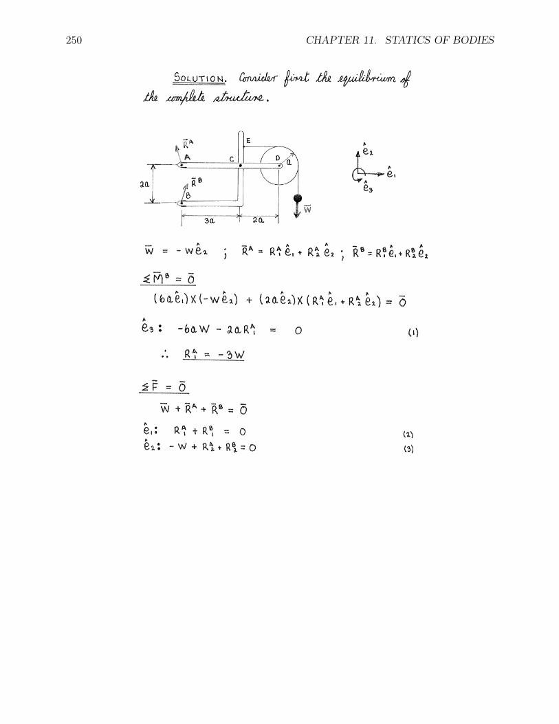
250 CHAPTER 11. STATICS OF BODIES

11.9. MORE EXAMPLES IN STATIC EQUILIBRIUM 251

252 CHAPTER 11. STATICS OF BODIES

11.9. MORE EXAMPLES IN STATIC EQUILIBRIUM 253
Example 83

254 CHAPTER 11. STATICS OF BODIES

11.9. MORE EXAMPLES IN STATIC EQUILIBRIUM 255

256 CHAPTER 11. STATICS OF BODIES

11.9. MORE EXAMPLES IN STATIC EQUILIBRIUM 257
Example 84

258 CHAPTER 11. STATICS OF BODIES

11.9. MORE EXAMPLES IN STATIC EQUILIBRIUM 259

260 CHAPTER 11. STATICS OF BODIES
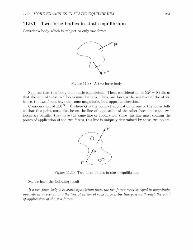
11.9. MORE EXAMPLES IN STATIC EQUILIBRIUM 261
11.9.1 Two force bodies in static equilibrium
Consider a body which is subject to only two forces.
Figure 11.38: A two force body
Suppose that this body is in static equilibrium. Then, consideration of ΣF = 0 tells usthat the sum of these two forces must be zero. Thus, one force is the negative of the other;hence, the two forces have the same magnitude, but, opposite direction.
Consideration of ΣMQ = 0 where Q is the point of application of one of the forces tellsus that this point must also be on the line of application of the other force; since the twoforces are parallel, they have the same line of application; since this line must contain thepoints of application of the two forces, this line is uniquely determined by these two points.
Figure 11.39: Two force bodies in static equilibrium
So, we have the following result.
If a two-force body is in static equilibrium then, the two forces must be equal in magnitude,opposite in direction, and the line of action of each force is the line passing through the pointof application of the two forces
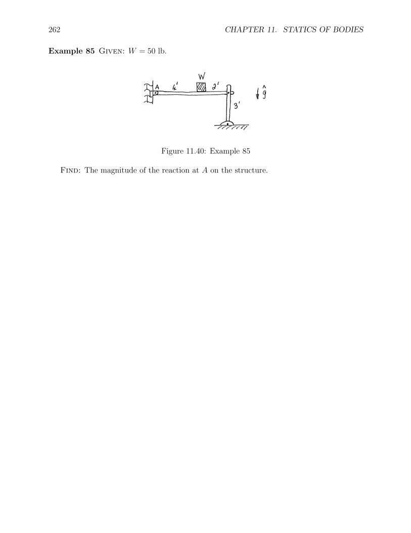
262 CHAPTER 11. STATICS OF BODIES
Example 85 Given: W = 50 lb.
Figure 11.40: Example 85
Find: The magnitude of the reaction at A on the structure.

11.9. MORE EXAMPLES IN STATIC EQUILIBRIUM 263
Example 86 Given: F = 250 N.
Figure 11.41: Example 86
Find: Reactions on the structure at B and C.

264 CHAPTER 11. STATICS OF BODIES
11.10 Statically indeterminate problems
A problem is statically determinate if one can solve for all the unknown forces and torquesusing only the conditions of static equilibrium: ΣF = 0 and ΣMQ = 0.
A problem is statically indeterminate if one cannot solve for all the unknown forces andtorques using only the conditions of static equilibrium: ΣF = 0 and ΣMQ = 0. To solve forall the forces an torques in such a problem, one usually has to use some information on thematerial properties of the bodies under study.
So there are three possibilities for a statics problem:
Statically determinate: Same number of unknowns as independent equations.
Statically indeterminate: More unknowns than independent equations.
Impossible: Less unknowns than independent equations.
These possibilities are illustrated in the following examples.

11.10. STATICALLY INDETERMINATE PROBLEMS 265
Example 87 (Statically indeterminate)
Figure 11.42: Example 87

266 CHAPTER 11. STATICS OF BODIES
Example 88 (Statically determinate)
Figure 11.43: Example 89

11.10. STATICALLY INDETERMINATE PROBLEMS 267
Example 89 (Statically determinate)
Figure 11.44: Example 89

268 CHAPTER 11. STATICS OF BODIES
Example 90 (Impossible)
Figure 11.45: Example 90

11.11. INTERNAL FORCES 269
11.11 Internal forces
11.12 Exercises
Exercise 32 Determine the reaction on the massless structure at pin joint A.
Exercise 33 Obtain a simple force system consisting of a single force or a single couplewhich is equivalent to the force system shown.

270 CHAPTER 11. STATICS OF BODIES

Chapter 12
Momentum
12.1 Linear momentum
•P
v
m
Suppose we are observing the motion of a particle of mass m moving with velocity vrelative to some inertial reference frame.
• The linear momentum of the particle in the inertial frame is defined by
L = mv
dim[L] = MLT−1 = FT
units: kg ms−1 or lb sec
Suppose ΣF is the sum of all the forces acting on the particle, i.e., ΣF =∑N
j=1 Fj, where
F1, F
2, . . . , F
Nare all the forces acting on the particle.
•P
1F–
F– 2
•••
F– N
271

272 CHAPTER 12. MOMENTUM
Then, using ΣF = ma we can obtain the following result for any inertial reference frame:
• The sum of the forces acting on a particle equals the time rate of change of the linearmomentum of the particle, i.e.,
∑
F = L
Proof. Since m is constant,
˙L =d
dt(mv)
= md
dt(v)
= ma
where a is the inertial acceleration of the particle. It now follows from ΣF = ma that
ΣF = L
12.2 Impulse of a force
12.2.1 Integral of a vector valued function
e2
e1
e3
Z (t)–
Suppose Z is a function of a scalar variable t and
Z = Z1e1 + Z2e2 + Z3e3
Consider any interval [t0, t1]. Relative to reference frame e, the integral of Z over [t0, t1] isdefined by
∫ t1
t0Z dt :=
(∫ t1
t0Z1 dt
)
e1 +(∫ t1
t0Z2 dt
)
e2 +(∫ t1
t0Z3 dt
)
e3

12.2. IMPULSE OF A FORCE 273
Example 91 SupposeZ(t) = e1 + te2 + sin te3
Then∫ 1
0Z dt =
(∫ 1
01 dt
)
e1 +(∫ 1
0t dt
)
e2 +(∫ 1
0sin t dt
)
e3
= e1 +1
2e2 + (1 − cos(1))e3
• Note that∫ t1
t0
˙Z dt = Z(t1) − Z(t0)
12.2.2 Impulse
• The impulse of a force F over a time interval [t0, t1] is defined by
I t1t0
:=∫ t1
t0F dt
Impulsive forces. Large magnitude over a short time interval. They usually occur duringimpacts and collisions.
Suppose we are observing the motion of a particle relative to some inertial reference frameover some time interval [t0, t1]. Let ∆L be the change in the linear momentum of the particleover the time interval, i.e,
∆L = L(t1) − L(t0)
Let ΣI be the total impulse acting on the particle over the time interval, i.e, ΣI is the sumof the impulses of all the forces acting on the particle:
ΣI =N∑
j=1
(∫ t1
t0F
jdt)
Then we have the following result for any inertial reference frame:
• Over any time interval, the total impulse acting on a particle equals the change in thelinear momentum of a particle, i.e.,
ΣI = ∆L
Proof. Recall thatΣF = ˙L

274 CHAPTER 12. MOMENTUM
Integrate over the time interval [t0, t1] to yield:
∫ t1
t0ΣF dt =
∫ t1
t0
˙L dt
We have
∫ t1
t0ΣF dt =
∫ t1
t0
N∑
j=1
Fj
dt
=N∑
j=1
(∫ t1
t0F
jdt)
= ΣI
∫ t1
t0
˙L dt = L(t1) − L(t0)
= ∆L
This yields the desired result.
We have the following immediate consequence of the above result.
• If the total impulse acting on a particle over any time interval [t0, t1] is zero, then thelinear momentum of the particle is conserved over that interval, i.e.,
L(t1) = L(t0)
From this it follows that the velocity is also conserved, i.e.,
v(t1) = v(t0)
This is also true for any compoment, i.e, if the total impulse has zero component in somedirection, then the corresponding components of the linear momentum and the velocity areconserved; see next example.

12.2. IMPULSE OF A FORCE 275
Example 92
Ball impacts smooth wall. Find the exit speed v.
Solution. Suppose the impact between wall and ball occurs over the interval [t0, t1].
Looking at a FBD of the ball during impact, the only force with a vertical component isweight. Its impulse is
∫ t1
t0mgg dt = mg(t1 − t0)g
Ideally, we can choose t1 − t0 arbitrarily small; so the impulse due ro the weight force isnegligible. Hence, the vertical component of the total impulse is zero. This implies that thevertical component of the ball’s velocity is preserved during impact, i.e.,
v cos(30) = 10 cos(60)
Hence,
v =10√
3ms−1

276 CHAPTER 12. MOMENTUM
12.3 Angular momentum
Suppose we are observing the motion of a particle of mass m relative to some inertial referenceframe i and Q is any point. Let r be the position of particle relative to Q and let ˙r be itstime derivative in i.
• The angular momentum of the particle about Q is defined by
HQ = r × m ˙r
dim[HQ] = ML2T−1 = FLT
units: kg m2 s−1 or lb ft sec
In the above definition, Q does not have to be a fixed point. Suppose Q = O where O is apoint fixed in the inertial reference frame; then
˙r = v
where v is the velocity of the particle in the frame; hence
HO = r × mv
= r × L
where L is the momentum of the particle in the inertial frame.
Example 93 Angular momentum and polar coordinates
We haver = rer
˙r = rω eθ

12.3. ANGULAR MOMENTUM 277
HenceHO = mr2ω e3
Suppose ΣMO is the sum of the moments about point O of all the forces acting on theparticle, i.e.,
ΣMO :=N∑
j=1
r × Fj
= r ×N∑
j=1
Fj
= r × ΣF
where r is the position of the particle relative to O. We have now the following result forany inertial reference frame:
• The time rate of change of the angular momentum of a particle about a fixed point O isequal to the sum of the moments about O of all the forces acting on the particle, i.e.,
∑
MO
= HO
Proof. Since m is constant,
HO
=dHO
dt
=d
dt(r × mr)
= ˙r × m ˙r + r × m¨r
= r × m¨r
Since O is fixed in frame i, the vector ¨r equals a, the inertial acceleration of the particle ini; since i is inertial we have ΣF = ma, hence
HO
= r × ΣF
= ΣMO
and we obtain the desired result.
Example 94 Simple pendulum

278 CHAPTER 12. MOMENTUM
12.4 Central force motion
Recall that a particle undergoes central force motion if is subject to a single force F whoseline of action always passes through some inertially fixed point O.
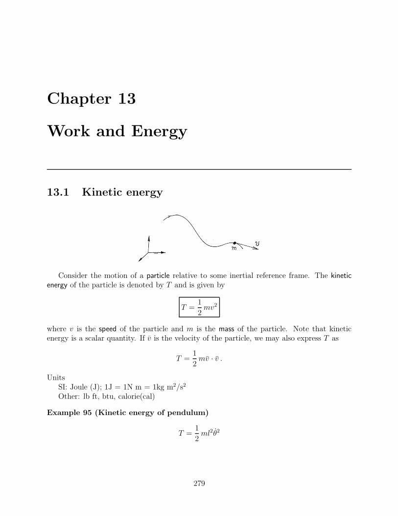
Chapter 13
Work and Energy
13.1 Kinetic energy
Consider the motion of a particle relative to some inertial reference frame. The kineticenergy of the particle is denoted by T and is given by
T =1
2mv2
where v is the speed of the particle and m is the mass of the particle. Note that kineticenergy is a scalar quantity. If v is the velocity of the particle, we may also express T as
T =1
2mv · v .
UnitsSI: Joule (J); 1J = 1N m = 1kg m2/s2
Other: lb ft, btu, calorie(cal)
Example 95 (Kinetic energy of pendulum)
T =1
2ml2θ2
279

280 CHAPTER 13. WORK AND ENERGY
Consider now a rigid body of mass m which is translating with speed v relative to someinertial reference frame. The kinetic energy of the body is simply the sum of the kineticenergies of the particles composing the body. Hence the kinetic energy of a translating rigidbody is also given by T = 1
2mv2 where m is the mass of the body.
13.2 Power
Consider a force F acting on a particle which is moving with velocity v relative to someinertial reference frame. The power of the force is denoted by P and is given by
P = F · v
UnitsSI: Watt (W); 1W = 1J/s = 1Nm/s = 1kg m2/s3
Other: hp; 1 hp = 550 ft lb/s =745.7 W
Consider now a rigid body which is translating with velocity v relative to some inertialreference frame. Suppose it is subject to a distributed force system whose resultant is F .Then the power of the distributed force system is defined to be the resultant of the powersof the forces which make up the force system. This power is also given by P = F · v.

13.2. POWER 281
Example 96 (Normal forces and friction)

282 CHAPTER 13. WORK AND ENERGY
Example 97 (Lift and drag)

13.3. A BASIC RESULT 283
13.3 A basic result
Consider a particle in motion relative to an inertial reference frame. We define theresultant power of all the forces acting on the particle to be the sum of the powers of all theforces acting on the particle. We have now the following result.
The resultant power of all the forces acting on a particle equals the time rate of changeof the kinetic energy of the particle.
Mathematically, we can represent the above result as
∑P = T
where∑P is the resultant power of all the forces acting on the particle and T is the kinetic
energy of the particle.
To prove the above result, recall that in an inertial reference frame we have
N∑
i=1
F i = ma
where a is the inertial acceleration of the particle and F1, · · · , FN are the forces acting onthe particle. Since the power of force F i is F i · v where v is the velocity of the particle inthe inertial frame, we have
∑
P =N∑
i=1
(F i · v) =
(
N∑
i=1
F i
)
· v = ma · v.
Also
T =d
dt
(
1
2mv · v
)
=1
2m ˙v · v +
1
2mv · ˙v = m ˙v · v = ma · v
It now follows that∑P = T .

284 CHAPTER 13. WORK AND ENERGY
Example 98 (The simple pendulum) Show that
θ +g
lsin θ = 0

13.4. CONSERVATIVE FORCES AND POTENTIAL ENERGY 285
13.4 Conservative forces and potential energy
Consider a force acting on a particle moving in some inertial reference frame. We say thatthis force is conservative, if there is a scalar function φ with the following properties:
(a) The function φ is only a function of the position of the particle relative to someinertially fixed point.
(b) The power of the force is the negative of the time rate of change of φ, that is
P = −φ
where P is the power of the force.
The function φ is called the potential energy of the force. So, we have the followingststement.
The power of a conservative force is the negative of the time rate of change of its potentialenergy.
13.4.1 Weight
Figure 13.1: Weight
φ = mgh
13.4.2 Linear springs
Figure 13.2: Linear spring
φ =1
2kx2

286 CHAPTER 13. WORK AND ENERGY
13.4.3 Inverse square gravitational force
Figure 13.3: Inverse square gravitational force
φ = −GMm
r
13.5 Total mechanical energy
Consider a particle in motion relative to some inertial reference frame. We can divide theforces acting on the particle into conservative forces and non-conservative forces. Associatedwith each conservative force is a potential energy. Let φ be the sum of the potential energiesof all the conservative forces. We call this the total potential energy. The total mechanicalenergy is the sum of the kinetic energy and the total potential energy, that is
E = T + φ
where E denotes the total mechanical energy.Let
∑c P be the resultant power of all the conservative forces. Since the power of aconservative force equals the negative of the time rate of change of its potential energy, itfollows that the resultant power of the conservative forces equals the negative of the timerate of change of the total potential energy, that is,
c∑
P = −φ .
Let∑nc P demote the resultant power of all the non-conservative forces. Then the resultant
power∑P of all the forces satisfies
∑
P =c∑
P +nc∑
P = −φ +nc∑
P .
Recalling that∑P = T , we have
−φ +nc∑
P = T .
Hencenc∑
P = T + φ
ornc∑
P = E .

13.5. TOTAL MECHANICAL ENERGY 287
The resultant power of all the nonconservative forces equals the time rate of change ofthe total mechanical energy.
So, if the resultant power of the nonconservative forces is zero, then the time rate ofchange of the mechanical energy is zero. In this case the energy E is constant and we saythat the total mechanical energy is conserved.

288 CHAPTER 13. WORK AND ENERGY
Example 99 (The simple pendulum) Show that
θ +g
lsin θ = 0

13.6. WORK 289
13.6 Work
Basically, work is the time integral of power. More specifically, consider any time interval[t1, t2]. Then the work done by a force over that interval is denoted by WD and is given by
WD =∫ t2
t1P dt
where P is the power of the force.We have now the following results:
∑
WD = ∆T
where ∆T = T (t2) − T (t1).Also,
nc∑
WD = ∆E
where ∆E = E(t2) − E(t1), that is,
the total work done by all the non-conservative forces equals the change in total energy
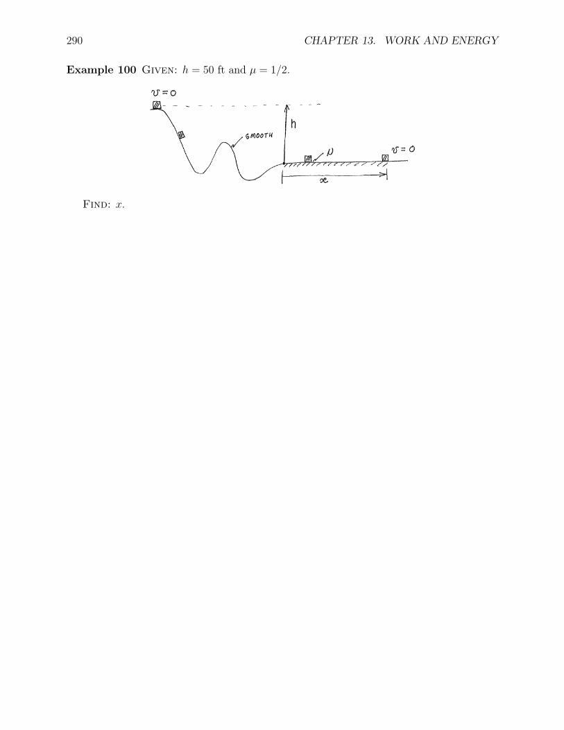
290 CHAPTER 13. WORK AND ENERGY
Example 100 Given: h = 50 ft and µ = 1/2.
Find: x.

Chapter 14
Systems of Particles
291