A4: Theoretical techniques and ideas

Ali Alavi

Part II Chemistry, Michaelmas 2006

I. RECAP OF HUCKEL THEORY

We begin with a brief recap of Huckel theory, taking initially the practical viewpoint of

‘how-to-do’ calculations, rather than the ‘meaning’ of the subject. We will later return to

this latter aspect. This approach, I hope, will have the advantage of getting you started on

familiar ground. Actually, Huckel theory is an archetype of more general molecular-orbital

theory, and even more widely, of many quantum mechanical principles. Therefore, a good

practical grasp of it proves invaluable in many areas of chemistry.

Let us start with the benzene molecule, the Huckel theory of which is very instructive. The

steps are as follows. To begin with, we suppose we can treat separately the π-electrons from

the σ-electrons. For planar molecules such as benzene, this assumption is strictly justifiable

on symmetry grounds, but we will nevertheless assume it to be true for non-planar molecules

as well. Next, we set up a “basis” of 6 pz (or, as we shall sometimes interchangeably refer to

them, as pπ) atomic orbitals, one for each carbon in the appropriate geometry. We will label

these atomic orbitals φ1, ..., φ6.

φ1

φ2φ3

φ4

φ5φ6

FIG. 1: The pπ atomic orbitals of benzene.

Our aim is to discover the linear combinations of these atomic orbitals which are somehow

‘optimal’. To do this, we assume that there is a Hamiltonian operator, H (which we will often

write simply as H), whose function it is to determine the energy of an electron, and roughly

speaking, can be decomposed into three terms: the kinetic energy of the electron, the potential

energy of the electron in the nuclear framework, and the potential energy of the electron due

1

to the average distribution of all other electrons. The precise mathematical form for this

effective Hamiltonian it is rather complicated (we will deal with it in C6); for the moment,

let us simply assume it exists, with matrix elements:

Hrs = 〈φr|H|φs〉 (1)

and not concern ourselves with the actual evaluation of these matrix elements (which is

generally speaking difficult, and except in a few cases must be done on the computer). One

of the beauties of Huckel theory is to assume a simple form for this Hamiltonian - and it

turns out that many of the general conclusions of Huckel theory are independent of the

actual numerical values of this matrix.

In addition to the Hamiltonian matrix, there is also an overlap matrix, which measures

the spatial overlap of the orbitals among each other:

Srs = 〈φr|φs〉 (2)

If our orbitals are normalised, then Srr = 1, and furthermore, if the orbitals are orthogonal

to each other, then Srs = 0 for r 6= s. To begin with, we will not make either assumption.

What we seek are linear combinations of these AO’s which are stationary solutions of the

Hamiltonian. These special linear combinations are the molecular orbitals. We can think

of them as standing “waves” whose (square) amplitudes given the probability of finding an

electron at that site. Among these waves, for example, is a solution which minimises the

energy of the Hamiltonian. We denote an MO with the symbol ψ, and write it as a linear

combination of AO’s whose coefficients cr have to be determined:

ψ =∑

r

crφr (3)

Consider the energy of this MO:

ǫ =〈ψ|H|ψ〉〈ψ|ψ〉 (4)

Expanding the sum, we get:

ǫ =

∑

rs c∗rcs〈φr|H|φs〉

∑

rs c∗rcs〈φr|φs〉

(5)

In almost all of the applications we will meet, the coefficients cr will be real numbers, and it

is not necessary to worry about the complex conjugation. In this case, the expression reduces

2

to:

ǫ =

∑

rs crcsHrs∑

rs crcsSrs(6)

Before we continue, let us briefly mention a word about the summation notation. The

double sum denoted above means:

∑

rs

≡N∑

r=1

N∑

s=1

(7)

where N is the number of sites in the molecule. Now, it is usually convenient to split the

sum up into two parts, terms for which r = s and terms for which r 6= s. Thus, assuming a

general summand ars:

∑

rs

ars =

N∑

r=1

arr +

N∑

r=1

N∑

s 6=r

ars (8)

The third step is that, in all our applications, the summand (ars) is symmetric:

ars = asr (9)

In this case, the remaining double sum can be further simplified:

∑

rs

ars =∑

r

arr + 2N∑

r=1

N∑

s>r

ars (10)

=∑

r

arr + 2N−1∑

r=1

N∑

s=r+1

ars (11)

which we compactly write as:

∑

rs

ars =∑

r

arr + 2∑

s>r

ars. (12)

The secular equations

We seek the coefficients cr such that the energy ǫ is optimised in the sense that the

first-derivative wrt cr all vanish, i.e.

∂ǫ

∂cr= 0 (13)

This is a fairly straightforward exercise in partial differentiation with the following fairly

simple result. The cr which satisfy the above are given by the matrix equation:

∑

r

(Hsr − ǫSsr)cr = 0 (14)

3

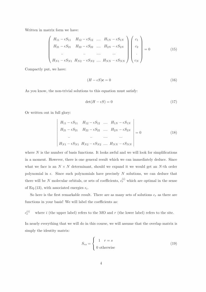
Written in matrix form we have:

H11 − ǫS11 H12 − ǫS12 .... H1N − ǫS1N

H21 − ǫS21 H22 − ǫS22 .... H2N − ǫS2N

.. .. .... ...

HN1 − ǫSN1 HN2 − ǫSN2 .... HNN − ǫSNN

c1

c2

.

cN

= 0 (15)

Compactly put, we have:

(H − ǫS)c = 0 (16)

As you know, the non-trivial solutions to this equation must satisfy:

det(H − ǫS) = 0 (17)

Or written out in full glory:

∣∣∣∣∣∣∣∣∣∣∣∣

H11 − ǫS11 H12 − ǫS12 .... H1N − ǫS1N

H21 − ǫS21 H22 − ǫS22 .... H2N − ǫS2N

.. .. .... ...

HN1 − ǫSN1 HN2 − ǫSN2 .... HNN − ǫSNN

∣∣∣∣∣∣∣∣∣∣∣∣

= 0 (18)

where N is the number of basis functions. It looks awful and we will look for simplifications

in a moment. However, there is one general result which we can immediately deduce. Since

what we face is an N × N determinant, should we expand it we would get an N -th order

polynomial in ǫ. Since such polynomials have precisely N solutions, we can deduce that

there will be N molecular orbitals, or sets of coefficients, c(i)r which are optimal in the sense

of Eq.(13), with associated energies ǫi.

So here is the first remarkable result. There are as many sets of solutions cr as there are

functions in your basis! We will label the coefficients as:

c(i)r where i (the upper label) refers to the MO and r (the lower label) refers to the site.

In nearly everything that we will do in this course, we will assume that the overlap matrix is

simply the identity matrix:

Srs =

1 r = s

0 otherwise(19)

4

On the face of it, this assumption is not easily defendable since the overlap between neigh-

bouring pz orbitals in benzene can be anywhere between 0.25 and 0.4. On the other hand, the

effect of including the proper overlap in qualitative terms turns out not to be very significant,

and since it simplifies life as regarding the solutions to the problem, we will proceed with it.

In this case, the Huckel secular equations substantially simplify:

∣∣∣∣∣∣∣∣∣∣∣∣

H11 − ǫ H12 .... H1N

H21 H22 − ǫ .... H2N

.. .. .... ...

HN1 HN2 .... HNN − ǫ

∣∣∣∣∣∣∣∣∣∣∣∣

= 0 (20)

Before we proceed with other simplifications associated with Huckel theory, let us state some

properties of the MO’s:

Orthogonality:∑

r

(c(i)r )∗c(j)r = 0 for i 6= j. (21)

[Note the complex conjugation in the above. It will usually have no effect because we normally

work with real orbitals. On occasion, complex orbitals do arise, particularly in ring systems,

and then you to have to take care]. In addition, it is strongly recommended that you always

work with normalised orbitals:

Normalisation:∑

r

|c(i)r |2 = 1 (22)

This condition ensures that the probability to find your electron somewhere on one of the N

sites must be unity [why?]. Having computed MO’s according to some method you should

check to see if each one is indeed normalised. If not, then the coefficients should be replaced

by:

c(i)r → c(i)r

(∑

r |c(i)r |2)1/2

(23)

Normalisation will be essential for computing a number of properties later on, such as bond-

orders, atomic populations, etc. In a normalised MO ψi, with orthogonal AOs, the probability

to find an electron on site r is:

p(i)r = |c(i)r |2 (24)

5

The Huckel assumptions

Now let us proceed by making certain assumptions which simplify actual calculations.

• We set all diagonal elements to be the same: Hii = α, irrespective of where the φi

occurs in the molecule. Clearly for benzene and other rings this is strictly true (not

an approximation), whereas in general it is not. We will later discuss what actual

numerical values α could be assigned (you will see experiment is not clear-cut on

this issue). Roughly speaking α measures the energy of the AO φ in the complete

framework of the molecule. It is often (somewhat misleadingly) called the Coulomb

integral, which is not correct since it also contains kinetic energy terms. In the limit of

the molecule being torn apart into its consitutent atoms, it is the energy of a p orbital.

Note, however, that in the molecule, it is not simply this energy, since the orbital also

sees the field due to the other nuclei (and electrons).

• We also set the off-diagonal elements between nearest-neighbour orbitals to be β, and

all others to be zero:

Hrs =

β r → s, i.e. if σ-bonded to each other

0 otherwise(25)

Thus, at the end of all this we have, for benzene, the following ‘secular’ determinant to solve:

∣∣∣∣∣∣∣∣∣∣∣∣∣∣∣∣∣∣

α− ǫ β 0 0 0 β

β α− ǫ β 0 0 0

0 β α− ǫ β 0 0

0 0 β α− ǫ β 0

0 0 0 β α− ǫ β

β 0 0 0 β α− ǫ

∣∣∣∣∣∣∣∣∣∣∣∣∣∣∣∣∣∣

= 0 (26)

You can see that we’ve eliminated a lot of elements, but we still appear to face a somewhat

daunting task of solving a 6×6 determinant. Actually we will see in another lecture how this

(and more generally, cyclic polyenes, and also linear chains) can be easily solved using some

nifty algebra, but for the moment we will appeal to another method which is more general

and which you’ve already had plenty of exposure at Part IB: using symmetry.

6

II. USING SYMMETRY TO SIMPLIFY THE SOLUTION OF HUCKEL

PROBLEMS

The point-group of the benzene molecule is D6h, and you will from last year’s experience

immediately be able to work out the irreducible representations spanned by the six pz orbitals:

D6h E 2C6 2C3 C2 3C ′2 3C ′′

2 i 2S3 2S6 σh 3σd 3σv

Γpz 6 0 0 0 −2 0 0 0 0 −6 0 2(27)

which can be reduced to

Γpz = B2g + E1g +A2u + E2u (28)

This means that we can setup 4 classes of symmetry adapted orbitals (which correspond to 4

irreducible representations of the D6h point group), 2 one-dimensional irreps (B2g and A2u)

and 2 two-dimensional irreps (E1g and E2u). In this basis (which we will shortly setup), the

Hamiltonian is in block-diagonal form:

E2u

E1g

A2u

B2g

FIG. 2: Block diagonal form of the benzene Hamiltonian

By inspection of character tables (or, more formally, using the projector operator), we can

write down the symmetry adapted orbitals:

φA2u=

1√6

(φ1 + φ2 + φ3 + φ4 + φ5 + φ6)

φB2g=

1√6

(φ1 − φ2 + φ3 − φ4 + φ5 − φ6)

φ(1)E2u

=1√12

(2φ1 − φ2 − φ3 + 2φ4 − φ5 − φ6)

φ(2)E2u

=1

2(φ2 − φ3 + φ5 − φ6)

φ(1)E1g

=1√12

(2φ1 + φ2 − φ3 − 2φ4 − φ5 + φ6)

φ(2)E1g

=1

2(φ2 + φ3 − φ5 − φ6)

7

B2g

E2u E2u

E1g E1g

A2u

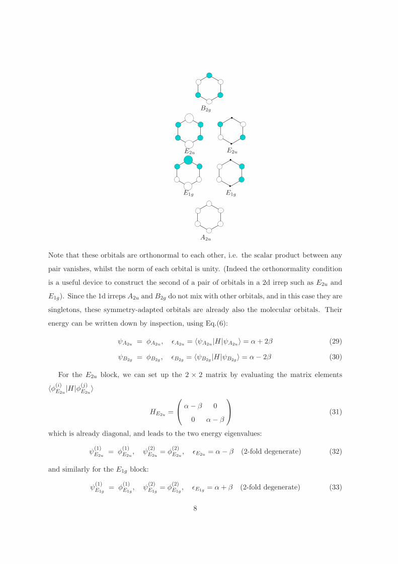
Note that these orbitals are orthonormal to each other, i.e. the scalar product between any

pair vanishes, whilst the norm of each orbital is unity. (Indeed the orthonormality condition

is a useful device to construct the second of a pair of orbitals in a 2d irrep such as E2u and

E1g). Since the 1d irreps A2u and B2g do not mix with other orbitals, and in this case they are

singletons, these symmetry-adapted orbitals are already also the molecular orbitals. Their

energy can be written down by inspection, using Eq.(6):

ψA2u= φA2u

, ǫA2u= 〈ψA2u

|H|ψA2u〉 = α+ 2β (29)

ψB2g= φB2g

, ǫB2g= 〈ψB2g

|H|ψB2g〉 = α− 2β (30)

For the E2u block, we can set up the 2 × 2 matrix by evaluating the matrix elements

〈φ(i)E2u

|H|φ(j)E2u

〉

HE2u=

α− β 0

0 α− β

(31)

which is already diagonal, and leads to the two energy eigenvalues:

ψ(1)E2u

= φ(1)E2u

, ψ(2)E2u

= φ(2)E2u

, ǫE2u= α− β (2-fold degenerate) (32)

and similarly for the E1g block:

ψ(1)E1g

= φ(1)E1g

, ψ(2)E1g

= φ(2)E1g

, ǫE1g= α+ β (2-fold degenerate) (33)

8

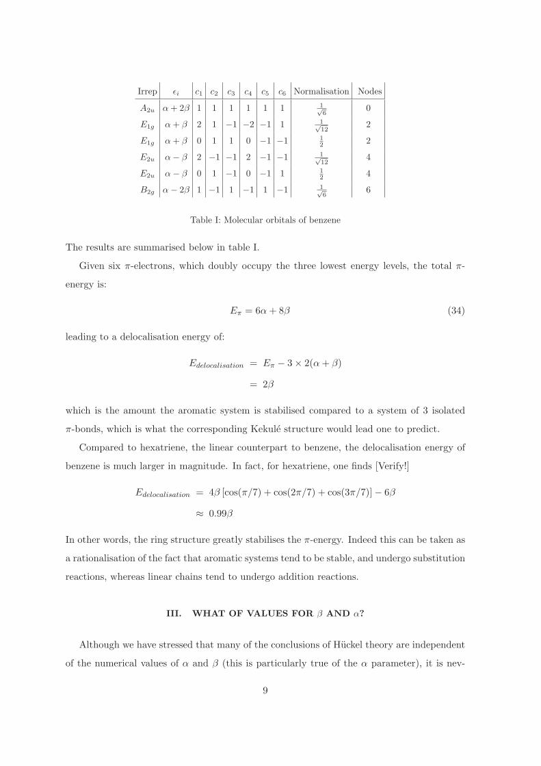
Irrep ǫi c1 c2 c3 c4 c5 c6 Normalisation Nodes

A2u α+ 2β 1 1 1 1 1 1 1√6

0

E1g α+ β 2 1 −1 −2 −1 1 1√12

2

E1g α+ β 0 1 1 0 −1 −1 1

22

E2u α− β 2 −1 −1 2 −1 −1 1√12

4

E2u α− β 0 1 −1 0 −1 1 1

24

B2g α− 2β 1 −1 1 −1 1 −1 1√6

6

Table I: Molecular orbitals of benzene

The results are summarised below in table I.

Given six π-electrons, which doubly occupy the three lowest energy levels, the total π-

energy is:

Eπ = 6α+ 8β (34)

leading to a delocalisation energy of:

Edelocalisation = Eπ − 3 × 2(α+ β)

= 2β

which is the amount the aromatic system is stabilised compared to a system of 3 isolated

π-bonds, which is what the corresponding Kekule structure would lead one to predict.

Compared to hexatriene, the linear counterpart to benzene, the delocalisation energy of

benzene is much larger in magnitude. In fact, for hexatriene, one finds [Verify!]

Edelocalisation = 4β [cos(π/7) + cos(2π/7) + cos(3π/7)] − 6β

≈ 0.99β

In other words, the ring structure greatly stabilises the π-energy. Indeed this can be taken as

a rationalisation of the fact that aromatic systems tend to be stable, and undergo substitution

reactions, whereas linear chains tend to undergo addition reactions.

III. WHAT OF VALUES FOR β AND α?

Although we have stressed that many of the conclusions of Huckel theory are independent

of the numerical values of α and β (this is particularly true of the α parameter), it is nev-

9

ertheless interesting to ask what type of experimental result could be used to yield values.

One idea is to use experimental delocalisation energies, which are tabulated for the series

benzene, naphthalene, anthracene and phenanthrene (the “zig-zag” form of anthracene):

(a) (b)

(c)

FIG. 3: (a) Naphthalene, (b) Anthracene and (c)Phenanthrene

Two conclusions can be drawn from this. First, the close parallel between the Huckel the-

Molecule Theory Experiment Estimate of β

Benzene 2β 37 (kcal/mol) 18.5 (kcal/mol)

Naphthalene 3.68β 75 (kcal/mol) 20.4 (kcal/mol)

Anthracene 5.32β 105 (kcal/mol) 19.7 (kcal/mol)

Phenanthrene 5.45β 110 (kcal/mol) 20.2 (kcal/mol)

Table II: Delocalisation energies.

ory prediction on the variation of the delocalisation energy for the series, as compared to

experiment, which indicates that even such crude calculations are able to reproduce a sig-

nificant trend. Taking β to be about -20 kcal/mol leads to a reasonable agreement between

predicted and experimental delocalisation energies; thus naphthalene is about twice as ad-

ditionally stable compared to the Kekule structures, as is benzene, and anthracene is about

three times as stable, etc. The second point regards the difference between anthracene and

phenanthrene, the latter being slightly more stable. Indeed, this trend continues for larger

systems: the annulation to give “zig-zag” forms are indeed experimentally more stable then

the corresponding linear ones (eg chrysene is more stable than tetracene). Thus our very

crude theory is able to give some interesting, semi-quantitative, results.

10

Matters look less rosy if we consider a different type of measurement of β, using ionisation

potentials. Recall that the first ionisation potential is the minimum energy required to remove

an electron from a molecule, and therefore it is reasonable to suppose that the electron

removed comes from HOMO. Since, according to Huckel theory, the energy of an orbital can

be written in the form:

ǫ = α+ xβ

where x is suitable coefficient which depends on the molecule, one may suppose that if we

take a series of molecules (eg benzene, naphthalene, anthracene, etc), for which the x can

be calculated, and plot the ionisation energy as a function of x, then the slope of such a

(hopefully linear) curve would yield β, whereas the intercept would yield α. It turns out that

a least-squares fit yields:

Experimental ionisation energy = −163 + (−57 ± 3.9)x kcal/mol (35)

i.e. a value of β ≈ −57 kcal/mol, which is more than twice that value obtained from the

delocalisation energies. In fact this turns out to be a quite general feature of Huckel theory.

Experiments which depend on the energy of single orbitals turn out to yield values of β

which are always roughly a factor of two larger that those bases on total energies, in which

the energies of many orbitals are summed together.

The explanation for this behaviour can be found by considering the manner in which

electron-electron interactions are dealt with in the Hamiltonian H. Recall that the H is an

effective Hamiltonian in which an electron sees the average field due to all other electrons.

In other words, electron 1 sees a field due to the average of electrons 2, 3 , etc, and this field,

in addition to the field due to the nuclear framework, determines the energy eigenvalue of

electron 1. Similarly, electron 2 sees the average field of electron 1, electron 3, etc, and its

energy eigenvalue reflects these interactions as well. Therefore, if we add the energy eigenvalue

of electron 1 and electron 2, we have counted twice the average electrostatic interaction

between electron 1 and electron 2. This is exactly what is done in our method of calculating

the total π-energy: we simply add the energy of all occupied levels. On the other hand, if

we are dealing with purely the energy of a single energy level, there is no double counting.

Therefore, it should not be surprising that methods used to estimate β based on the total

energies yield values about 1/2 of that from ionisation potential experiments.

11

IV. SOME SPECIAL SYSTEMS: LINEAR CHAINS AND RINGS OF ARBITRARY

LENGTH

In two general cases, it is possible to solve the Huckel equations to get the energy levels

and molecular orbital coefficients with little ado. Consider first a cyclic polyene (ring) of N

atomic sites. In such a ring, site r is connected to sites r + 1 and r − 1, with the boundary

1 23

i− 1ii+ 1

i+ 2

N

FIG. 4: A cyclic polyene of length N

condition

c(n)r = c

(n)N+r. (36)

In the above, n signifies the molecular orbital label. A row in the Huckel equations is:

(α− ǫn)c(n)r + β(c

(n)r+1 + c

(n)r−1) = 0 (37)

Let us guess the following solution:

c(n)r = ei2πnr/N (38)

(which, you should note, satisfies the boundary condition Eq.(36)), and insert into Eq.(37):

(α− ǫn)ei2πnr/N + β(ei2πn(r+1)/N + ei2πn(r−1)/N ) = 0 (39)

Notice that one can factorise ei2πnr/N and hence cancel this term, leaving an equation which

no longer involves the site r:

(α− ǫn) + β(ei2πn/N + e−i2πn)/N ) = 0 (40)

i.e.:

ǫn = α+ 2β cos(2πn/N) (41)

12

α

α2β

α+ 2β

α+ 2β

α− 2β

α− 2β

FIG. 5: The energy levels of the first few cyclic polyenes.

where n runs from 0,±1,±2..., N/2 for even-N or n = 0,±1,±2, ...,±(N − 1)/2 for odd-N .

There are always precisely N MO’s. Since the cos(x) is an even function, this implies that,

apart from n = 0 and n = N/2, the energy levels come in degenerate pairs. The energy levels

for the first few cyclic polyenes are be represented in Fig. 5.

This structure of the energy levels of the cyclic polyenes has an interesting consequence,

leading to the Huckel 4N +2 rule. Consider the sequence of cyclic polyenes with N = 3 to 7:

C3H3: In the neutral molecule, there are 3 π-electrons. However, owing to the energy level

pattern, the third electron occupies an anti-bonding orbital. Therefore, one would expect that

the cation C3H+3 to be more stable than the neutral species, and therefore that it should be

easy to remove an electron from the molecule.

C4H4. In this molecule, there are a two degenerate non-bonding orbitals, which in the

neutral species are partially occupied. According to Hund’s first rule, the expected electronic

configuration is a triplet state. However, this is the case to be expected only if the molecule is

indeed square planar. In fact a distortion of the molecular geometry can occur. As a result,

cyclobutadiene takes on a rectangular structure, in which the bonds alternate in length,

(long-short-long-short).

13

replacemen

α

α+ 2β

α− 2β βlβs

βl − βs

−βl + βs

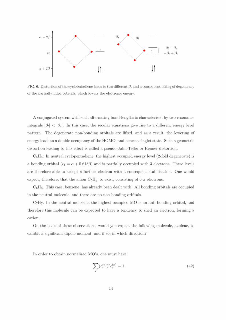
FIG. 6: Distortion of the cyclobutadiene leads to two different β, and a consequent lifting of degeneracy

of the partially filled orbitals, which lowers the electronic energy.

A conjugated system with such alternating bond-lengths is characterised by two resonance

integrals |βl| < |βs|. In this case, the secular equations give rise to a different energy level

pattern. The degenerate non-bonding orbitals are lifted, and as a result, the lowering of

energy leads to a double occupancy of the HOMO, and hence a singlet state. Such a geometric

distortion leading to this effect is called a pseudo-Jahn-Teller or Renner distortion.

C5H5: In neutral cyclopentadiene, the highest occupied energy level (2-fold degenerate) is

a bonding orbital (ǫ1 = α + 0.618β) and is partially occupied with 3 electrons. These levels

are therefore able to accept a further electron with a consequent stabilisation. One would

expect, therefore, that the anion C5H−5 to exist, consisting of 6 π electrons.

C6H6. This case, benzene, has already been dealt with. All bonding orbitals are occupied

in the neutral molecule, and there are no non-bonding orbitals.

C7H7. In the neutral molecule, the highest occupied MO is an anti-bonding orbital, and

therefore this molecule can be expected to have a tendency to shed an electron, forming a

cation.

On the basis of these observations, would you expect the following molecule, azulene, to

exhibit a significant dipole moment, and if so, in which direction?

In order to obtain normalised MO’s, one must have:

∑

r

(c(n)r )∗c(n)

r = 1 (42)

14

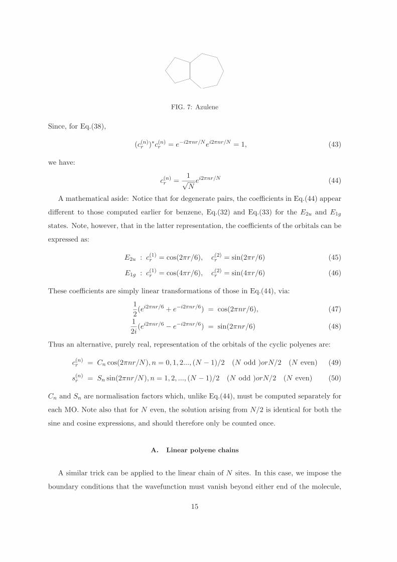
FIG. 7: Azulene

Since, for Eq.(38),

(c(n)r )∗c(n)

r = e−i2πnr/Nei2πnr/N = 1, (43)

we have:

c(n)r =

1√Nei2πnr/N (44)

A mathematical aside: Notice that for degenerate pairs, the coefficients in Eq.(44) appear

different to those computed earlier for benzene, Eq.(32) and Eq.(33) for the E2u and E1g

states. Note, however, that in the latter representation, the coefficients of the orbitals can be

expressed as:

E2u : c(1)r = cos(2πr/6), c(2)r = sin(2πr/6) (45)

E1g : c(1)r = cos(4πr/6), c(2)r = sin(4πr/6) (46)

These coefficients are simply linear transformations of those in Eq.(44), via:

1

2(ei2πnr/6 + e−i2πnr/6) = cos(2πnr/6), (47)

1

2i(ei2πnr/6 − e−i2πnr/6) = sin(2πnr/6) (48)

Thus an alternative, purely real, representation of the orbitals of the cyclic polyenes are:

c(n)r = Cn cos(2πnr/N), n = 0, 1, 2..., (N − 1)/2 (N odd )orN/2 (N even) (49)

s(n)r = Sn sin(2πnr/N), n = 1, 2, ..., (N − 1)/2 (N odd )orN/2 (N even) (50)

Cn and Sn are normalisation factors which, unlike Eq.(44), must be computed separately for

each MO. Note also that for N even, the solution arising from N/2 is identical for both the

sine and cosine expressions, and should therefore only be counted once.

A. Linear polyene chains

A similar trick can be applied to the linear chain of N sites. In this case, we impose the

boundary conditions that the wavefunction must vanish beyond either end of the molecule,

15

1

2

i− 1

i

i+ 1

N − 1

N

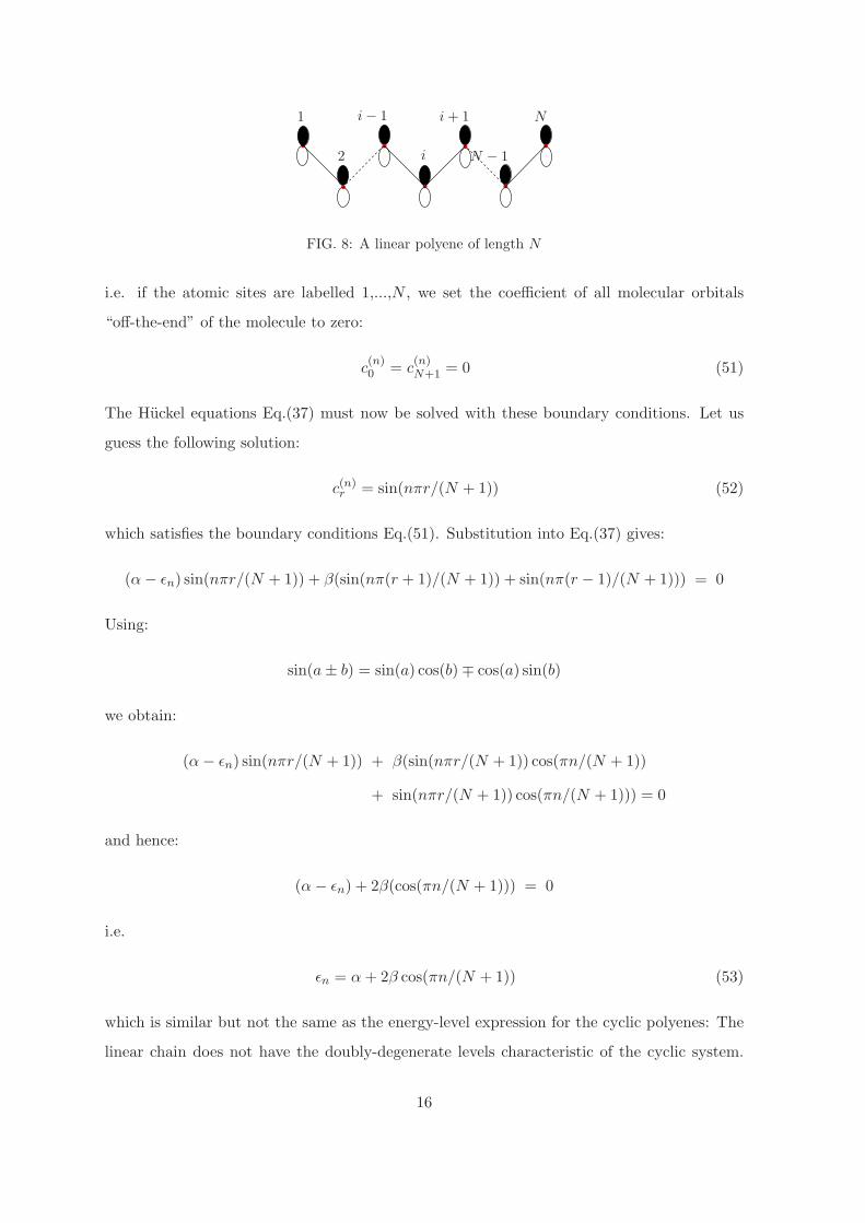
FIG. 8: A linear polyene of length N

i.e. if the atomic sites are labelled 1,...,N , we set the coefficient of all molecular orbitals

“off-the-end” of the molecule to zero:

c(n)0 = c

(n)N+1 = 0 (51)

The Huckel equations Eq.(37) must now be solved with these boundary conditions. Let us

guess the following solution:

c(n)r = sin(nπr/(N + 1)) (52)

which satisfies the boundary conditions Eq.(51). Substitution into Eq.(37) gives:

(α− ǫn) sin(nπr/(N + 1)) + β(sin(nπ(r + 1)/(N + 1)) + sin(nπ(r − 1)/(N + 1))) = 0

Using:

sin(a± b) = sin(a) cos(b) ∓ cos(a) sin(b)

we obtain:

(α− ǫn) sin(nπr/(N + 1)) + β(sin(nπr/(N + 1)) cos(πn/(N + 1))

+ sin(nπr/(N + 1)) cos(πn/(N + 1))) = 0

and hence:

(α− ǫn) + 2β(cos(πn/(N + 1))) = 0

i.e.

ǫn = α+ 2β cos(πn/(N + 1)) (53)

which is similar but not the same as the energy-level expression for the cyclic polyenes: The

linear chain does not have the doubly-degenerate levels characteristic of the cyclic system.

16

Ring

bonding

nonbonding

antibonding

4βE = α

N = 3 N = 4 N = 5 N = 6

N ∞

Chain

bonding

nonbonding

antibonding

4βE = α

N = 2 N = 3 N = 4 N = 5 N = 6 N ∞

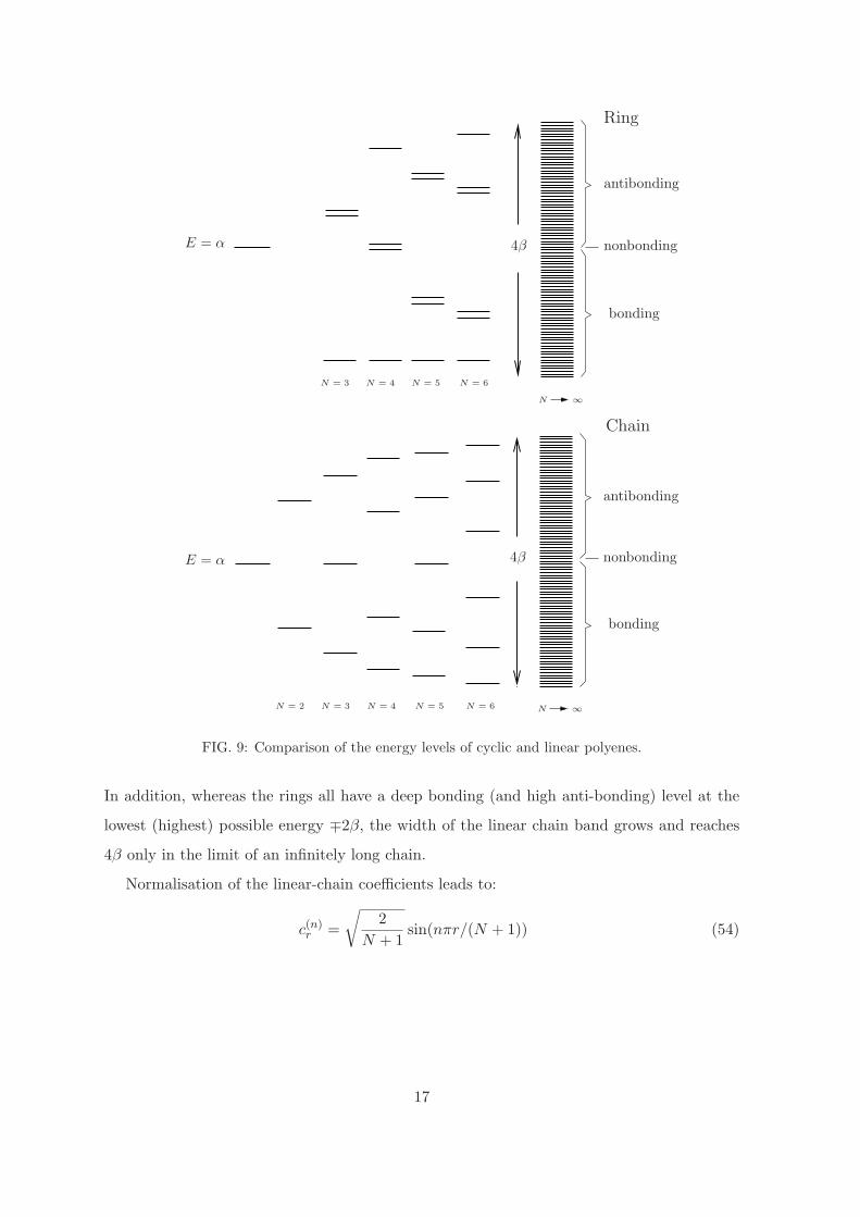
FIG. 9: Comparison of the energy levels of cyclic and linear polyenes.

In addition, whereas the rings all have a deep bonding (and high anti-bonding) level at the

lowest (highest) possible energy ∓2β, the width of the linear chain band grows and reaches

4β only in the limit of an infinitely long chain.

Normalisation of the linear-chain coefficients leads to:

c(n)r =

√

2

N + 1sin(nπr/(N + 1)) (54)

17

V. POPULATIONS AND BOND ORDERS

The solutions to the Huckel equations yield molecular orbitals, which are typically de-

localised over the entire molecule. One might ask about the typical electronic charge on a

given site as a result of populating certain MO’s, and to ask if there is a measure of the

bonding/anti-bonding interaction between a pair of atoms.

A reasonable definition of the total π-electron population at atomic site r is:

qr =∑

i

fi|c(i)r |2 (55)

where the sum runs over the orbitals, fi is the occupation of the orbital, i.e. 2,1, or 0, for

doubly, singly and unoccupied levels, and c(i)r is the coefficient of the ith orbital (normalised

of course) on the rth site. This expression is using that fact that, in MO i, the π-electron

density at site r is |c(i)r |2. [Take care, if using complex orbitals, to use the square-magnitude

of the orbital, not simply its square].

If the MOs are all either doubly occupied, or empty, (which is case for closed-shell

molecules), then the expression for the populations reduces to:

qr = 2∑

i∈occ

|c(i)r |2 (Closed shell molecules) (56)

where the notation i ∈ occ implies that you sum only over the occupied MOs.

A bond order between two atomic sites, r, s can be analogously defined by:

prs =

∑

i

fi1

2

(c(i)r )∗c(i)s + c(i)r (c(i)s )∗

︸ ︷︷ ︸

complexconjugate

(57)

=∑

i

fic(i)r c(i)s for real orbitals (58)

The rationale for this is that c(i)r c

(i)s can be thought of as a “bonding charge” in MO i between

sites r and s, which can be positive (accumulation), negative (depletion) or zero.

As for populations, for closed-shell molecules the bond-order has a simpler form:

prs = 2∑

i∈occ

c(i)r c(i)s (closed shell molecule with real orbitals) (59)

As a first example, let us compute the populations and bond orders in benzene. In this

case, since all atomic sites are equivalent, we need compute the population for one site only.

Taking site 1, and using the MOs in Table I:

q1 = 2

[1

6+

4

12+ 0

]

= 1

18

You should explicitly verify that the charges on the other sites are likewise equal to one. Note

also that the use of the complex version of the MOs would have given you the same result:

q1 =1

6

(

1 × 2 + ei2π/6e−i2π/6 × 2 + ei4π/6e−i4π/6 × 2)

= 1

For the bond orders we obtain:

p12 = 2

[1

6+

2√12

× 1√12

]

=2

3

In other words, in benzene, each atomic site has the same electron density residing on it,

and a π-bond-order of 2/3 between nearest neighbour sites.

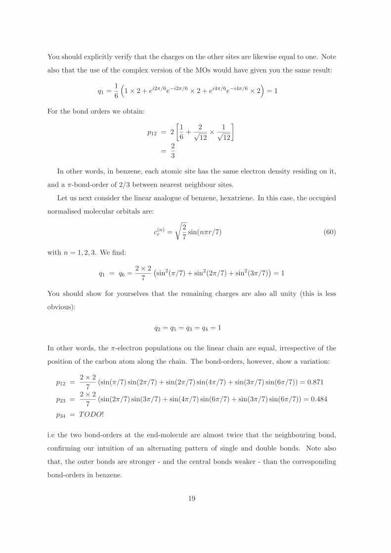
Let us next consider the linear analogue of benzene, hexatriene. In this case, the occupied

normalised molecular orbitals are:

c(n)r =

√

2

7sin(nπr/7) (60)

with n = 1, 2, 3. We find:

q1 = q6 =2 × 2

7

(sin2(π/7) + sin2(2π/7) + sin2(3π/7)

)= 1

You should show for yourselves that the remaining charges are also all unity (this is less

obvious):

q2 = q5 = q3 = q4 = 1

In other words, the π-electron populations on the linear chain are equal, irrespective of the

position of the carbon atom along the chain. The bond-orders, however, show a variation:

p12 =2 × 2

7(sin(π/7) sin(2π/7) + sin(2π/7) sin(4π/7) + sin(3π/7) sin(6π/7)) = 0.871

p23 =2 × 2

7(sin(2π/7) sin(3π/7) + sin(4π/7) sin(6π/7) + sin(3π/7) sin(6π/7)) = 0.484

p34 = TODO!

i.e the two bond-orders at the end-molecule are almost twice that the neighbouring bond,

confirming our intuition of an alternating pattern of single and double bonds. Note also

that, the outer bonds are stronger - and the central bonds weaker - than the corresponding

bond-orders in benzene.

19

VI. ALTERNANT HYDROCARBONS

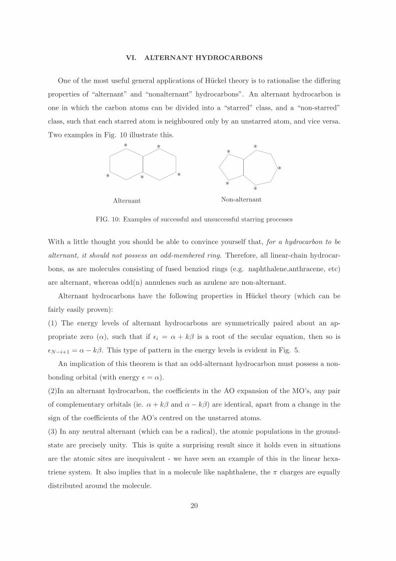
One of the most useful general applications of Huckel theory is to rationalise the differing

properties of “alternant” and “nonalternant” hydrocarbons”. An alternant hydrocarbon is

one in which the carbon atoms can be divided into a “starred” class, and a “non-starred”

class, such that each starred atom is neighboured only by an unstarred atom, and vice versa.

Two examples in Fig. 10 illustrate this.

Alternant Non-alternant

*

*

**

*

**

* *

*

FIG. 10: Examples of successful and unsuccessful starring processes

With a little thought you should be able to convince yourself that, for a hydrocarbon to be

alternant, it should not possess an odd-membered ring. Therefore, all linear-chain hydrocar-

bons, as are molecules consisting of fused benziod rings (e.g. naphthalene,anthracene, etc)

are alternant, whereas odd(n) annulenes such as azulene are non-alternant.

Alternant hydrocarbons have the following properties in Huckel theory (which can be

fairly easily proven):

(1) The energy levels of alternant hydrocarbons are symmetrically paired about an ap-

propriate zero (α), such that if ǫi = α + kβ is a root of the secular equation, then so is

ǫN−i+1 = α− kβ. This type of pattern in the energy levels is evident in Fig. 5.

An implication of this theorem is that an odd-alternant hydrocarbon must possess a non-

bonding orbital (with energy ǫ = α).

(2)In an alternant hydrocarbon, the coefficients in the AO expansion of the MO’s, any pair

of complementary orbitals (ie. α+ kβ and α− kβ) are identical, apart from a change in the

sign of the coefficients of the AO’s centred on the unstarred atoms.

(3) In any neutral alternant (which can be a radical), the atomic populations in the ground-

state are precisely unity. This is quite a surprising result since it holds even in situations

are the atomic sites are inequivalent - we have seen an example of this in the linear hexa-

triene system. It also implies that in a molecule like naphthalene, the π charges are equally

distributed around the molecule.

20

Proofs of some or all of these statements may be provided during the lectures. Otherwise

they should be considered as most interesting exercises.

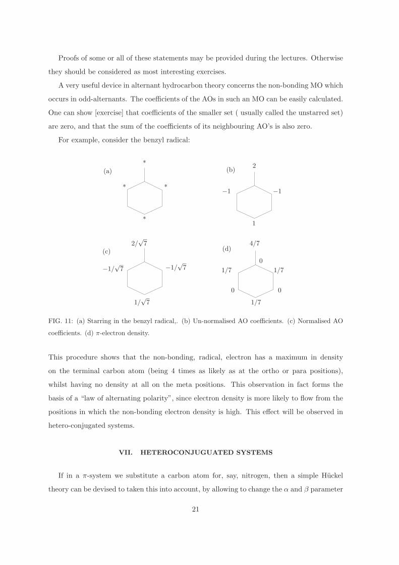
A very useful device in alternant hydrocarbon theory concerns the non-bonding MO which

occurs in odd-alternants. The coefficients of the AOs in such an MO can be easily calculated.

One can show [exercise] that coefficients of the smaller set ( usually called the unstarred set)

are zero, and that the sum of the coefficients of its neighbouring AO’s is also zero.

For example, consider the benzyl radical:

*

*

*

* 2

−1 −1

1

1/√

7

−1/√

7−1/√

7

2/√

7

1/7

1/7 1/7

4/7

0

0 0

(a) (b)

(c) (d)

FIG. 11: (a) Starring in the benzyl radical,. (b) Un-normalised AO coefficients. (c) Normalised AO

coefficients. (d) π-electron density.

This procedure shows that the non-bonding, radical, electron has a maximum in density

on the terminal carbon atom (being 4 times as likely as at the ortho or para positions),

whilst having no density at all on the meta positions. This observation in fact forms the

basis of a “law of alternating polarity”, since electron density is more likely to flow from the

positions in which the non-bonding electron density is high. This effect will be observed in

hetero-conjugated systems.

VII. HETEROCONJUGUATED SYSTEMS

If in a π-system we substitute a carbon atom for, say, nitrogen, then a simple Huckel

theory can be devised to taken this into account, by allowing to change the α and β parameter

21

associated with that site.

The α parameter for atom r, which is related to the Hamiltonian via αr = 〈φr|H|φr〉, can

be regarded as a measure of the electron-attracting ability of an atom, i.e. it is related to the

electronegativity of the atom in question. It is conventional to express the difference in α for

an atom r and compared to that of carbon in units of β (taking β between two neighbouring

carbon-atoms as the standard), i.e. β ≡ βCC , to write:

αr − αC = hβ, or αr = αC + hβ

The value of h is the defining parameter, which must be chosen with regard to the nature of

the substituent. For example, consider pyridine and pyrrole:

H

NN

6π6π

Pyridine Pyrrole

FIG. 12: The π system of pyridine and pyrrole

The N atom in pyridine is sp2 hybridised, with two of the hybrid orbitals forming σ

bonds with the neighbouring C atoms, and the third hybrid forming a lone pair. This leaves

one electron, which is donated into the π-network. In pyrrole, however, the N is also sp2

hybridised, but this time the presence of an H bonded to the N means that the N can donate

2 electrons into the π-network.

As an example, let us solve for Huckel equations for pyridine, taking αN = α+ 1.5β, and

22

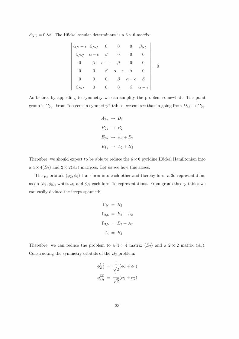
βNC = 0.8β. The Huckel secular determinant is a 6 × 6 matrix:

∣∣∣∣∣∣∣∣∣∣∣∣∣∣∣∣∣∣

αN − ǫ βNC 0 0 0 βNC

βNC α− ǫ β 0 0 0

0 β α− ǫ β 0 0

0 0 β α− ǫ β 0

0 0 0 β α− ǫ β

βNC 0 0 0 β α− ǫ

∣∣∣∣∣∣∣∣∣∣∣∣∣∣∣∣∣∣

= 0

As before, by appealing to symmetry we can simplify the problem somewhat. The point

group is C2v. From “descent in symmetry” tables, we can see that in going from D6h → C2v,

A2u → B2

B2g → B2

E2u → A2 +B2

E1g → A2 +B2

Therefore, we should expect to be able to reduce the 6× 6 pyridine Huckel Hamiltonian into

a 4 × 4(B2) and 2 × 2(A2) matrices. Let us see how this arises.

The pz orbitals (φ2, φ6) transform into each other and thereby form a 2d representation,

as do (φ3, φ5), whilst φ3 and φN each form 1d-representations. From group theory tables we

can easily deduce the irreps spanned:

ΓN = B2

Γ2,6 = B2 +A2

Γ3,5 = B2 +A2

Γ4 = B2

Therefore, we can reduce the problem to a 4 × 4 matrix (B2) and a 2 × 2 matrix (A2).

Constructing the symmetry orbitals of the B2 problem:

φ(1)B2

=1√2(φ2 + φ6)

φ(2)B2

=1√2(φ3 + φ5)

23

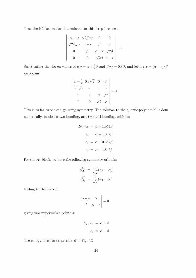
Thus the Huckel secular determinant for this irrep becomes:

∣∣∣∣∣∣∣∣∣∣∣∣

αN − ǫ√

2βNC 0 0√

2βNC α− ǫ β 0

0 β α− ǫ√

2β

0 0√

2β α− ǫ

∣∣∣∣∣∣∣∣∣∣∣∣

= 0

Substituting the chosen values of αN = α+ 12β and βNC = 0.8β, and letting x = (α− ǫ)/β,

we obtain:∣∣∣∣∣∣∣∣∣∣∣∣

x− 12 0.8

√2 0 0

0.8√

2 x 1 0

0 1 x√

2

0 0√

2 x

∣∣∣∣∣∣∣∣∣∣∣∣

= 0

This is as far as one can go using symmetry. The solution to the quartic polynomial is done

numerically, to obtain two bonding, and two anti-bonding, orbitals:

B2 : ǫ1 = α+ 1.954β

ǫ2 = α+ 1.062β,

ǫ3 = α− 0.667β,

ǫ4 = α− 1.845β

For the A2 block, we have the following symmetry orbitals:

φ(1)A2

=1√2(φ2 − φ6)

φ(2)A2

=1√2(φ3 − φ5)

leading to the matrix:

∣∣∣∣∣∣

α− ǫ β

β α− ǫ

∣∣∣∣∣∣

= 0

giving two unperturbed orbitals:

A2 : ǫ5 = α+ β

ǫ6 = α− β

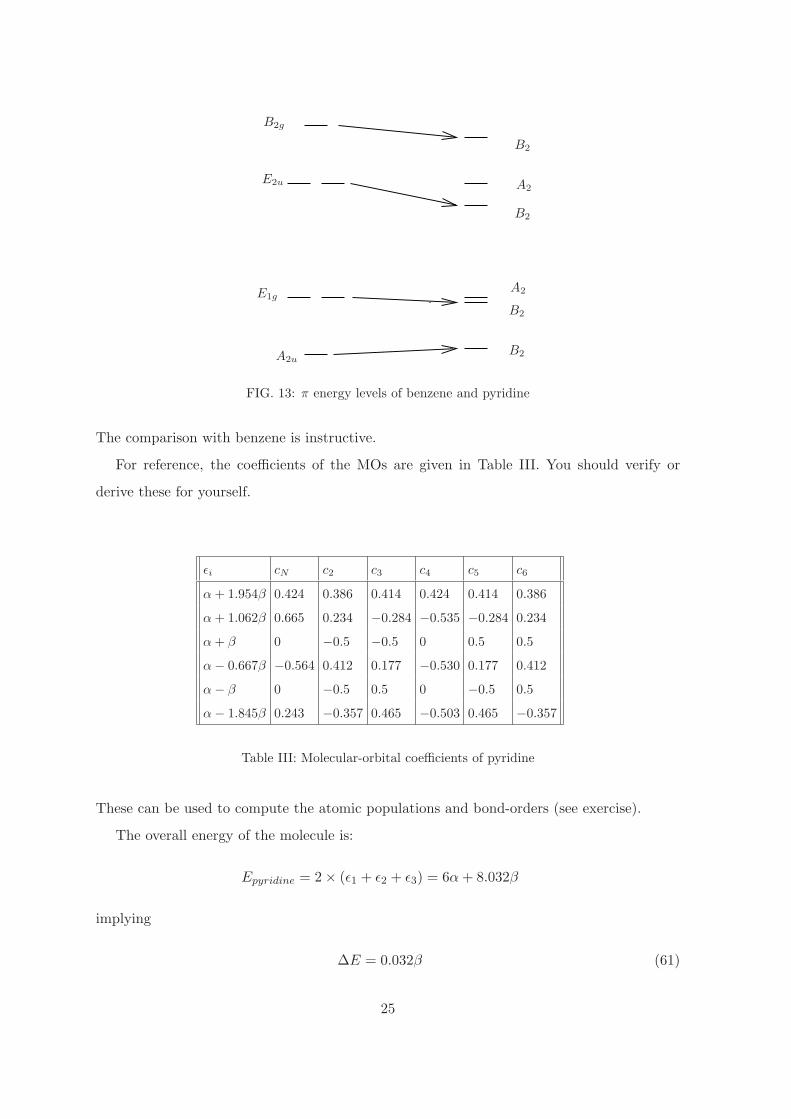
The energy levels are represented in Fig. 13

24

A2u

E1g

E2u

B2g

B2

B2

B2

B2

A2

A2

FIG. 13: π energy levels of benzene and pyridine

The comparison with benzene is instructive.

For reference, the coefficients of the MOs are given in Table III. You should verify or

derive these for yourself.

ǫi cN c2 c3 c4 c5 c6

α+ 1.954β 0.424 0.386 0.414 0.424 0.414 0.386

α+ 1.062β 0.665 0.234 −0.284 −0.535 −0.284 0.234

α+ β 0 −0.5 −0.5 0 0.5 0.5

α− 0.667β −0.564 0.412 0.177 −0.530 0.177 0.412

α− β 0 −0.5 0.5 0 −0.5 0.5

α− 1.845β 0.243 −0.357 0.465 −0.503 0.465 −0.357

Table III: Molecular-orbital coefficients of pyridine

These can be used to compute the atomic populations and bond-orders (see exercise).

The overall energy of the molecule is:

Epyridine = 2 × (ǫ1 + ǫ2 + ǫ3) = 6α+ 8.032β

implying

∆E = 0.032β (61)

25

We shall shortly develop an approximate, but much easier method, to compute approxi-

mately the energy levels and eigenstates of hetero-conjugated systems based on perturbation

theory.

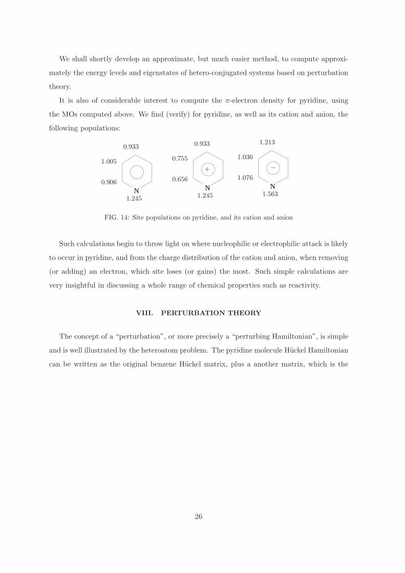
It is also of considerable interest to compute the π-electron density for pyridine, using

the MOs computed above. We find (verify) for pyridine, as well as its cation and anion, the

following populations:

N N N0.906

1.005

1.2451.245

0.656

0.755

0.9330.933

+

1.563

1.076

1.036

1.213

−

FIG. 14: Site populations on pyridine, and its cation and anion

Such calculations begin to throw light on where nucleophilic or electrophilic attack is likely

to occur in pyridine, and from the charge distribution of the cation and anion, when removing

(or adding) an electron, which site loses (or gains) the most. Such simple calculations are

very insightful in discussing a whole range of chemical properties such as reactivity.

VIII. PERTURBATION THEORY

The concept of a “perturbation”, or more precisely a “perturbing Hamiltonian”, is simple

and is well illustrated by the heteroatom problem. The pyridine molecule Huckel Hamiltonian

can be written as the original benzene Huckel matrix, plus a another matrix, which is the

26

perturbation:

Hpryidine =

αN βNC 0 0 0 βNC

βNC α β 0 0 0

0 β α β 0 0

0 0 β α β 0

0 0 0 β α β

βNC 0 0 0 β α

=

α β 0 0 0 β

β α β 0 0 0

0 β α β 0 0

0 0 β α β 0

0 0 0 β α β

β 0 0 0 β α

︸ ︷︷ ︸

Hbenzene

+

β2 −0.2β 0 0 0 −0.2β

−0.2β 0 0 0 0 0

0 0 0 0 0 0

0 0 0 0 0 0

0 0 0 0 0 0

−0.2β 0 0 0 0 0

︸ ︷︷ ︸

U

(62)

(where we have assumed αN = α+ β/2 and βNC = 0.8β). You see that in the present case,

the perturbing matrix has non-zero elements only along the first row and column, which

results from the fact only one site, namely the N, was changed.

More generally, suppose we are given a Hamiltonian H, which we can divide into two

parts, H(0) and U , where H(0) is the reference Hamiltonian whose energy levels and MO’s

we have already calculated, and U is the perturbation:

H = H(0) + U (63)

One can ask the question: assuming the perturbing Hamiltonian is “small”, how can one

express, even if only approximately, the energy levels and MOs of the perturbed Hamiltonian

(e.g. Hpyridine) in terms of the unperturbed one, (e.g. Hbenzene)?

Actually this is a very general and important topic which forms a entire lecture course in

itself (B7). Perturbation theory has an extraordinary number of applications. We will not

have the time to dwell into it in great detail, but will present the main results, and not derive

them in any rigorous way.

27

Change in energy levels

If the energy level ǫi is non-degenerate and the corresponding MO is given by ψi, then the

(first-order) change in energy induced by the perturbation is:

∆ǫ(1)i = 〈ψi|U |ψi〉 (64)

In terms of the coefficients c(i)r of the MO this is:

∆ǫ(1)i =

∑

r

|c(i)r |2Urr +∑

r 6=s

(c(i)r )∗c(i)s Urs

=∑

r

|c(i)r |2Urr +∑

r>s

(c(i)r )∗c(i)s Urs + c(i)r (c(i)s )∗(Usr)∗

=∑

r

|c(i)r |2Urr + 2∑

r>s

c(i)r c(i)s Urs [For real orbitals] (65)

For degenerate levels (eg the E1g and E2u levels of benzene), the same formula holds as long

as you have checked that the off-diagonal matrix elements of the perturbing Hamiltonian are

zero. In other words, if ψi and ψj are a degenerate pair, then as long as

〈ψi|U |ψj〉 = 0 (66)

the first order change in energy is given by Eq.(65). If the degenerate pair do not satisfy this

condition, then it is necessary to do something more complicated. More on this later.

As an example, let us consider the pyridine molecule, taking benzene to be the unperturbed

molecule. First, consider the lowest energy level:

ψ1 =1√6

(φ1 + φ2 + φ3 + φ4 + φ5 + φ6)

i.e. the coefficients are c(1)r = 1/

√6 for all sites. The energy of this state is ǫ1 = α+ 2β.

According to Eq.(65), the first-order change energy in going from benzene to pyridine is:

∆ǫ(1)1 = 〈ψ1|U |ψ1〉 =

1

6

(β

2− 0.2β × 2 × 2

)

= −0.05β

Therefore, the energy of this state is:

ǫ1 ≈ α+ 1.95β, [EXACTǫ1 = α+ 1.954β]

The error compared to the exact value is only approximately 0.2%.

28

Consider next the degenerate pair

ψ2 =1√12

(2φ1 + φ2 − φ3 − 2φ4 − φ5 + φ6)

ψ3 =1

2(φ2 + φ3 − φ5 − φ6)

Now, for the combination above, you can verify that:

〈ψ2|U |ψ3〉 = 0

Therefore, we can proceed directly to compute the first order change in energy:

∆ǫ(1)2 =

1

12

(

4 × β

2+ 2 × 2 × (−0.2β) × 2

)

= 0.033β

∆ǫ(1)3 = 0

i.e.:

ǫ2 ≈ α+ 1.033β, [EXACT = α+ 1.062β]

ǫ3 = α+ β, [EXACT = α+ β] (67)

In other words, the lowering of the B2 level is underestimated, whilst its originally degenerate

partner is left unperturbed (exact).

The total change of energy predicted by first-order perturbation theory is:

∆E(1) = (−0.05 × 2 + 0.033 × 2)β = −0.033β (68)

which is not very accurate, since it implies that the energy of pyridine has increased (more

positive), whereas the exact result shows a decrease of 0.032. This inaccuracy can be traced

to the above-noted underestimation of the perturbation of the E1g level. For better accuracy,

one needs higher-order perturbation theory. Fortunately, the comparison between the total

energies of benzene and pyridine tends not be so important, and so this lack of accuracy does

not detract from the usefulness of even 1st order perturbation theory.

If the degenerate pair of levels which are being perturbed do not satisfy the condition:

U12 = 〈ψ1|U |ψ2〉 = 0, then one needs to solve the following secular equation for the first-order

change ∆ǫ(1):

∣∣∣∣∣∣

U11 − ∆ǫ(1) U12

U21 U22 − ∆ǫ(1)

∣∣∣∣∣∣

= 0

29

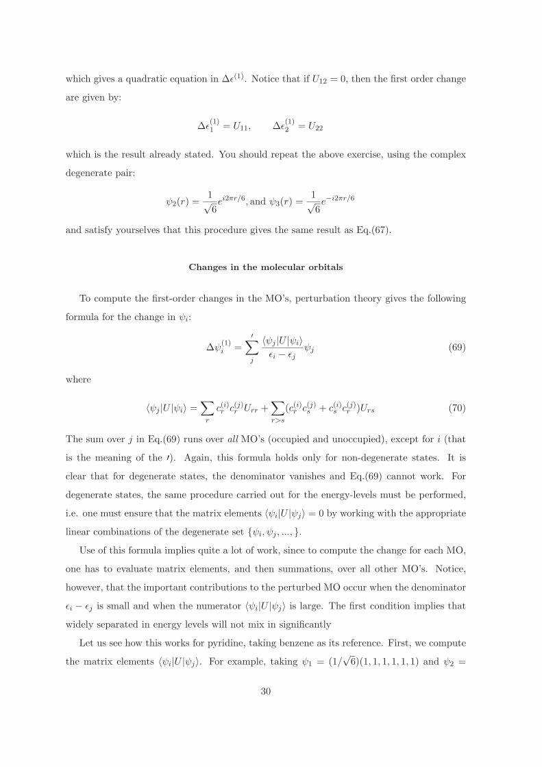
which gives a quadratic equation in ∆ǫ(1). Notice that if U12 = 0, then the first order change

are given by:

∆ǫ(1)1 = U11, ∆ǫ

(1)2 = U22

which is the result already stated. You should repeat the above exercise, using the complex

degenerate pair:

ψ2(r) =1√6ei2πr/6, and ψ3(r) =

1√6e−i2πr/6

and satisfy yourselves that this procedure gives the same result as Eq.(67).

Changes in the molecular orbitals

To compute the first-order changes in the MO’s, perturbation theory gives the following

formula for the change in ψi:

∆ψ(1)i =

′∑

j

〈ψj |U |ψi〉ǫi − ǫj

ψj (69)

where

〈ψj |U |ψi〉 =∑

r

c(i)r c(j)r Urr +∑

r>s

(c(i)r c(j)s + c(i)s c(j)r )Urs (70)

The sum over j in Eq.(69) runs over all MO’s (occupied and unoccupied), except for i (that

is the meaning of the ′). Again, this formula holds only for non-degenerate states. It is

clear that for degenerate states, the denominator vanishes and Eq.(69) cannot work. For

degenerate states, the same procedure carried out for the energy-levels must be performed,

i.e. one must ensure that the matrix elements 〈ψi|U |ψj〉 = 0 by working with the appropriate

linear combinations of the degenerate set {ψi, ψj , ..., }.Use of this formula implies quite a lot of work, since to compute the change for each MO,

one has to evaluate matrix elements, and then summations, over all other MO’s. Notice,

however, that the important contributions to the perturbed MO occur when the denominator

ǫi − ǫj is small and when the numerator 〈ψi|U |ψj〉 is large. The first condition implies that

widely separated in energy levels will not mix in significantly

Let us see how this works for pyridine, taking benzene as its reference. First, we compute

the matrix elements 〈ψi|U |ψj〉. For example, taking ψ1 = (1/√

6)(1, 1, 1, 1, 1, 1) and ψ2 =

30

(1/√

12)(2, 1,−1,−2,−1, 1), we have:

〈ψ1|U |ψ2〉 =1√

6 × 12

(

1 1 1 1 1 1)

β2 −0.2β 0 0 0 −0.2β

−0.2β 0 0 0 0 0

0 0 0 0 0 0

0 0 0 0 0 0

0 0 0 0 0 0

−0.2β 0 0 0 0 0

2

1

−1

−2

−1

1

=1√

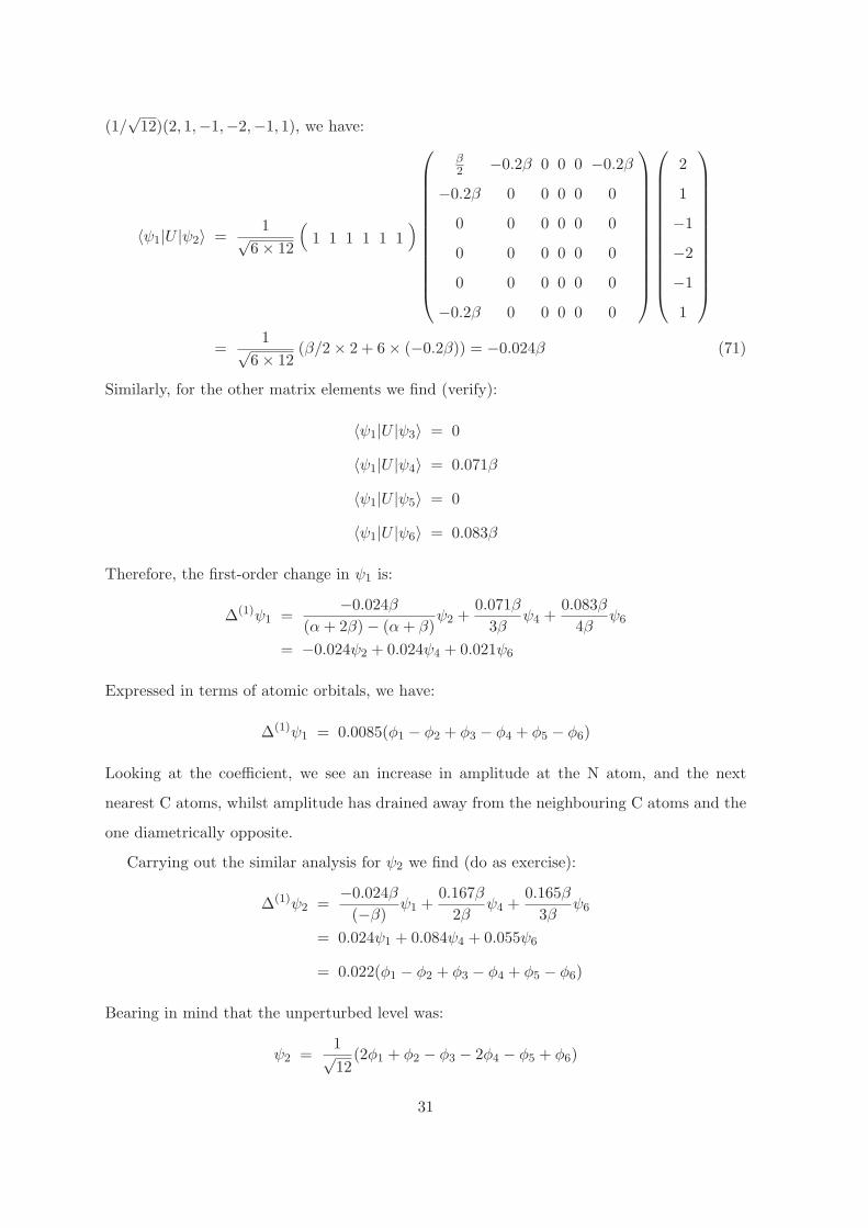
6 × 12(β/2 × 2 + 6 × (−0.2β)) = −0.024β (71)

Similarly, for the other matrix elements we find (verify):

〈ψ1|U |ψ3〉 = 0

〈ψ1|U |ψ4〉 = 0.071β

〈ψ1|U |ψ5〉 = 0

〈ψ1|U |ψ6〉 = 0.083β

Therefore, the first-order change in ψ1 is:

∆(1)ψ1 =−0.024β

(α+ 2β) − (α+ β)ψ2 +

0.071β

3βψ4 +

0.083β

4βψ6

= −0.024ψ2 + 0.024ψ4 + 0.021ψ6

Expressed in terms of atomic orbitals, we have:

∆(1)ψ1 = 0.0085(φ1 − φ2 + φ3 − φ4 + φ5 − φ6)

Looking at the coefficient, we see an increase in amplitude at the N atom, and the next

nearest C atoms, whilst amplitude has drained away from the neighbouring C atoms and the

one diametrically opposite.

Carrying out the similar analysis for ψ2 we find (do as exercise):

∆(1)ψ2 =−0.024β

(−β)ψ1 +

0.167β

2βψ4 +

0.165β

3βψ6

= 0.024ψ1 + 0.084ψ4 + 0.055ψ6

= 0.022(φ1 − φ2 + φ3 − φ4 + φ5 − φ6)

Bearing in mind that the unperturbed level was:

ψ2 =1√12

(2φ1 + φ2 − φ3 − 2φ4 − φ5 + φ6)

31

we see that the amplitude on N has further increased, and also on C atom 4. Thus the

expected changes in charge density are increases on N, decreases on the two neighbouring C’s,

and smaller changes on more distant C atoms. This is as observed in the exactly computed

π populations, Fig. 14.

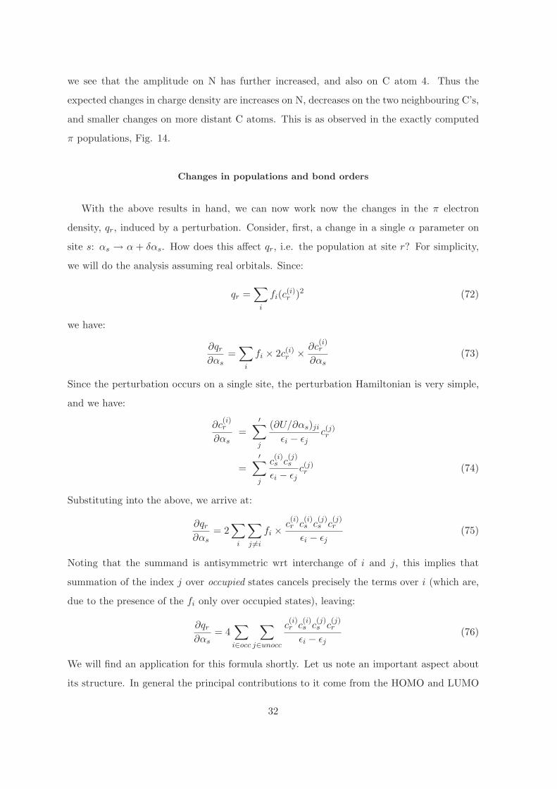
Changes in populations and bond orders

With the above results in hand, we can now work now the changes in the π electron

density, qr, induced by a perturbation. Consider, first, a change in a single α parameter on

site s: αs → α + δαs. How does this affect qr, i.e. the population at site r? For simplicity,

we will do the analysis assuming real orbitals. Since:

qr =∑

i

fi(c(i)r )2 (72)

we have:

∂qr∂αs

=∑

i

fi × 2c(i)r × ∂c(i)r

∂αs(73)

Since the perturbation occurs on a single site, the perturbation Hamiltonian is very simple,

and we have:

∂c(i)r

∂αs=

′∑

j

(∂U/∂αs)ji

ǫi − ǫjc(j)r

=′∑

j

c(i)s c

(j)s

ǫi − ǫjc(j)r (74)

Substituting into the above, we arrive at:

∂qr∂αs

= 2∑

i

∑

j 6=i

fi ×c(i)r c

(i)s c

(j)s c

(j)r

ǫi − ǫj(75)

Noting that the summand is antisymmetric wrt interchange of i and j, this implies that

summation of the index j over occupied states cancels precisely the terms over i (which are,

due to the presence of the fi only over occupied states), leaving:

∂qr∂αs

= 4∑

i∈occ

∑

j∈unocc

c(i)r c

(i)s c

(j)s c

(j)r

ǫi − ǫj(76)

We will find an application for this formula shortly. Let us note an important aspect about

its structure. In general the principal contributions to it come from the HOMO and LUMO

32

states, since in this case the denominator is smallest. In many cases, one can draw qualita-

tively correct conclusions by focusing exclusively on the ’action’ at the HOMO and LUMO.

In the literature, you will sometimes come across the term “self-polarisability” and “mutual

polarisability”, which describe the diagonal and off-diagonal elements, and are denoted by πr

and πrs respectively:

πr =∂qr∂αr

, (77)

πrs =∂qr∂αs

(78)

As an example, let us calculate the change in the π electron density on the N atom in

pyridine induced by a change ∆αN = β/2 using this formula. Here we have (it is helpful to

consult Table I at this point!):

∂qN∂αN

= 43∑

i=1

6∑

j=4

c(i)N c

(i)N c

(j)N c

(j)N

ǫi − ǫj

= 4

1

6

4

12 × 3β︸ ︷︷ ︸

i=1,j=4

+1

6 × 4β︸ ︷︷ ︸

i=1,j=6

+4

12

4

12 × 2β︸ ︷︷ ︸

i=2,j=4

+1

6 × 3β︸ ︷︷ ︸

i=2,j=6

= 4

[1

54β+

1

144β+

1

18β+

1

54β

]

=0.40

β(79)

Overall, therefore:

∆qN ≈ ∂qN∂αN

∆αN

= 0.20

which, looking at Fig. 14 (the exact value is 0.245), is a reasonable answer. [Bear in mind

that we have not yet considered the possible change in density induced by the change in β.

We come to this shortly.]

Notice that, according to Eq.(75), a negative change in the α of a site always leads to

an accumulation of electron density at that site. This is a general result of the perturbation

theory.

One can similarly work out the change in bond-order prs between two sites r and s, due to

a change in Htu (the same change must occur in Hut to keep things symmetric). For example

33

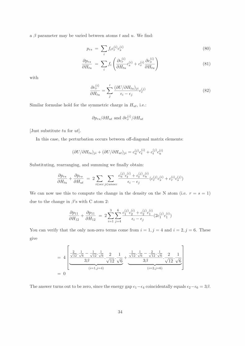
a β parameter may be varied between atoms t and u. We find:

prs =∑

i

fic(i)r c(i)s (80)

∂prs

∂Htu=∑

i

fi

(

∂c(i)r

∂Htuc(i)s + c(i)r

∂c(i)s

∂Htu

)

(81)

with

∂c(i)r

∂Htu=

′∑

j

(∂U/∂Htu)ji

ǫi − ǫjc(j)r (82)

Similar formulae hold for the symmetric charge in Hut, i.e.:

∂prs/∂Hut and ∂c(i)r /∂Hut

[Just substitute tu for ut].

In this case, the perturbation occurs between off-diagonal matrix elements:

(∂U/∂Htu)ji + (∂U/∂Hut)ji = c(j)u c(i)t + c

(j)t c(i)u

Substituting, rearranging, and summing we finally obtain:

∂prs

∂Htu+∂prs

∂Hut= 2

∑

i∈occ

∑

j∈unocc

c(j)u c

(i)t + c

(j)t c

(i)u

ǫi − ǫj(c(j)r c(i)s + c(i)r c(j)s )

We can now use this to compute the change in the density on the N atom (i.e. r = s = 1)

due to the change in β’s with C atom 2:

∂p11

∂H12+∂p11

∂H12= 2

3∑

i=1

6∑

j=4

c(j)1 c

(i)2 + c

(j)2 c

(i)1

ǫi − ǫj(2c

(j)1 c

(i)1 )

You can verify that the only non-zero terms come from i = 1, j = 4 and i = 2, j = 6. These

give

= 4

2√12. 1√

6− 1√

12. 1√

6

3β.

2√12.

1√6

︸ ︷︷ ︸

(i=1,j=4)

+

1√12. 1√

6− 2√

12. 1√

6

3β.

2√12.

1√6

︸ ︷︷ ︸

(i=2,j=6)

= 0

The answer turns out to be zero, since the energy gap ǫ1−ǫ4 coincidentally equals ǫ2−ǫ6 = 3β.

34

Differential form for the energy

It is possible to cast the expression for the total energy in a useful form in term of the

populations and bond-orders. Since:

E =∑

i∈occ

ǫi

=∑

i

fiǫi (83)

and for real normalised orbitals:

ǫi = 〈ψi|H|ψi〉

= 〈∑

r

c(i)r φr|H|∑

s

c(i)s φs〉

=∑

r

c(i)r c(i)r 〈φr|H|φr〉 +∑

r 6=s

c(i)r c(i)s 〈φr|H|φs〉

=∑

r

|c(i)r |2αr +∑

r 6=s

c(i)r c(i)s Hrs

=∑

r

|c(i)r |2αr + 2∑

r>s

c(i)r c(i)s Hrs (84)

where by writing αr and Hrs we have explicitly allowed for the possible variation of the α’s

along the molecule, and β’s between specific pairs of sites. The sums of r and r, s refer to

sums over atomic sites. Noting that:

∑

i

fi|c(i)r |2 = qr

∑

i

fic(i)r c(i)s = prs

Substituting into Eq.(83) and switching the order of summations, we obtain:

E =∑

i

fi

(∑

r

|c(i)r |2αr + 2∑

r>s

c(i)r c(i)s Hrs

)

=∑

r

qrαr + 2∑

r>s

prsHrs (85)

The usefulness of this expression stems from the fact that we can estimate changes in the

total energy induced by changes in the α or β’s. Taking αr and Hrs as independently variable

parameters, we can obtain the derivatives of the total energy wrt to them:

∂E

∂αr= qr

∂E

∂Hrs= 2prs

35

In other words, the first-order change in the energy for variations in the α and β of ∆αr and

∆Hrs can be written as:

∆E(1) =∑

r

qr∆αr + 2∑

r>s

prs∆Hrs (86)

Using this expression, we can immediately write down the first-order change in the energy of

hetero-substituted molecules, where we vary one or a few of the α’s and β’s.

For example, in pyridine, we changed one α → αN = α + 12β, and two of the β → 0.8β.

According to Eq.(86), we have:

∆E(1) =1

2β × 1 +

2

3× 2 × 2 × (−0.2β) = −0.033β

which can be compared with the first-order perturbation value Eq.(68) and exact diagonali-

sation exact value, Eq.(61).

A second-order correction to the energy can also be sought in which we account for the

variation in qr ( and in principle prs) upon a variation in αr (and Hrs). Thus, in the first

instance, we have:

∆E(2) =1

2

∂qN∂αN

∆α2N

Having computed this quantity in Eq.(79), we obtain for the 2nd order correction:

∆E(2) =1

2.0.4

β.β

2.β

2= 0.05β

This leads to an energy 6α+ 8.017β, which is closer to the exact value 6α+ 8.032β.

IX. REACTIVITY THEORY

An important use of the differential form of the energy, Eq.(86), regards its use in assessing

the reactivity of different sites of a conjugated molecule, towards attack by different types of

regents (electrophilic, nucleophilic and homolytic).

Let us start with an interpretation of the first term of Eq.(86), assuming a single site, r

is being approached by a reagent. If the regent is an electrophile, it will have the effect of

withdrawing electrons from site r, and therefore, in effect be reducing (making more negative)

the value of α. Assuming that no other perturbation occurs, we have therefore that the change

in energy is:

∆E ≈ qr∆αr (87)

36

For an electrophile, since ∆αr < 0, this implies that the largest lowering of energy occurs at

sites with the largest population. Conversely, for a nucleophile, we can assume that electrons

are pushed away from site r, leading effectively to a positive ∆αr, and therefore, nucleophilic

attack will most likely occur at sites with the smallest population, q.

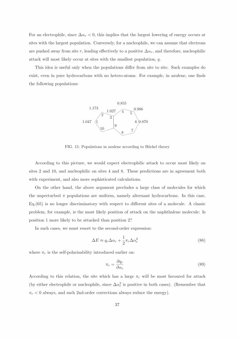
This idea is useful only when the populations differ from site to site. Such examples do

exist, even in pure hydrocarbons with no hetero-atoms. For example, in azulene, one finds

the following populations:

1.047

1.1731.027

0.855

0.986

0.8701

23

4 5

6

78

910

FIG. 15: Populations in azulene according to Huckel theory

According to this picture, we would expect electrophilic attack to occur most likely on

sites 2 and 10, and nucleophilic on sites 4 and 8. These predictions are in agreement both

with experiment, and also more sophisticated calculations.

On the other hand, the above argument precludes a large class of molecules for which

the unperturbed π populations are uniform, namely alternant hydrocarbons. In this case,

Eq.(65) is no longer discriminatory with respect to different sites of a molecule. A classic

problem, for example, is the most likely position of attack on the naphthalene molecule: Is

position 1 more likely to be attacked than position 2?

In such cases, we must resort to the second-order expression:

∆E ≈ qr∆αr +1

2πr∆α

2r (88)

where πr is the self-polarisability introduced earlier on:

πr =∂qr∂αr

(89)

According to this relation, the site which has a large πr will be most favoured for attack

(by either electrophile or nucleophile, since ∆α2r is positive in both cases). (Remember that

πr < 0 always, and such 2nd-order corrections always reduce the energy).

37

(a) (b)

(c) (d)

1

2

Y H

s t

0.584 0.732

0.603

2/√

11

−2/√

111/√

11

1/√

11

−1/√

11

2/√

8

1/√

81/√

8−1/

√8

−1/√

8

FIG. 16: (a) Naphthalene, bonds-orders from 1st order perturbation theory, (b) Transition complex;

(c) Residual molecule with site 1 removed and (d) Site 2 removed, showing the coefficients of the

non-bonding MO

We had earlier derived a general formula for computing πr, Eq.(76). The main difficulty

is that this equation is awkward to use, since the MOs which appear in this equation refer to

the unperturbed - but nevertheless perhaps very complicated - molecule, eg. the unperturbed

naphthalene molecule. In practice, we might have to resort to a ’perturbation theory of a

perturbation theory’, with a consequent reduction in accuracy.

There is a simplification which occurs if the β’s are all identical (like naphthalene). In

this case, to an excellent approximation, one can show:

πr =2qr − q2r2Nrβ

(90)

where Nr is the sum over the bond-orders of the sites attached to r:

Nr =∑

s→r

prs (91)

Nr is sometimes known as Dewar’s reactivity number, or ’bond number’. (We prefer the

latter term). According to this relation, πr increases as Nr decreases, i.e. sites involved

with the least bonding are the most polarisable and hence prone to attack. This equation

can sometimes be used if the bond-orders of the molecule are known. For example, for

38

naphthalene, perturbation theory gives the bond-orders indicated on Fig. 16, from which we

can conclude that site 1 would be marginally preferred to site 2 in a substitution reaction.

In fact, the Nr, the bond-number index, is also very useful is assessing the likely position

of homolytic attack, e.g. by a neutral radical. In this case the reagent is uncharged, which

means that the electric fields are likely to be small, and hence the approach of the attacking

molecule will not substantially affect the α’s. On the other hand, as it approaches and begins

to interact with the molecule, it is likely to weaken the bonds in the neighbourhood of the

site being attacked, and therefore increase (i.e. make more positive) the neighbouring β’s. In

this case, the second set of term in Eq.(86) come into play:

∆E ≈ 2∑

s→r

prs∆β = 2Nr∆β (92)

In other words, the sites with smallest Nr are, once again, most favourable to this type of

attack.

Localisation theory

There is a related approach to assessing reactivity, which is based on the idea of a “tran-

sition complex”, i.e. a point near the peak of the potential energy curve describing the

interaction between the molecule and reagent. For an attack on different positions, the peak

heights will in general differ, and the one with the lowest peak will generally be the favoured

pathway. How can we estimate the energy of the transition complex, relative to the unper-

turbed molecule (and reagent)?

Let us assume that the site under attack, r, is taken out of the conjugated π system by

the tetrahedrally-coordinated transition complex develops. The local sp2 geometry at site

r will be destroyed, and therefore the π-system itself will be affected, since the previously

delocalised MO’s will no longer be able to include a finite amplitude on this site. In other

words, the “volume” available to π-bonding will be reduced, and there will be a consequent

affect on the energy. The change in energy due to this reduction will, however, depend on

the position of attack. Therefore, we define a “localisation energy”, Lr, to be the difference

in π-energy of the residual molecule, Er consisting of n π-electrons, and original molecule E:

Lr = Er − E (93)

To compute the localisation energy, therefore, requires us to compute the energy of the

39

ψnb φr

2δ

FIG. 17: Energy level diagram of a residual odd-alternant, showing interaction with the non-bonding

MO or site r.

residual molecule in which site r has been removed from consideration. This is, in general,

quite a tedious task, but for even alternant hydrocarbons a simple (though approximate)

route exists to compute directly the difference in energy required by Eq.(93).

The key point is that the residual molecule must be a odd-alternant, and therefore must

possess a non-bonding MO, which we shall denote ψnb, and whose energy is α. To a good

approximation, the interaction between the fragment molecule and the site r (which also has

energy α) can be considered to be a two level problem, in which the matrix element between

them is given by:

H12 = 〈ψnb|H|φr〉

= (c(nb)s + c

(nb)t )β

where sites t and s are neighbouring to r, and c(nb)s and c

(nb)t are the coefficients of the

non-bonding MO at these two sites. Since we know the The secular determinant for such a

two-level system gives the energy, δ which arises out of the mixing of these two states:∣∣∣∣∣∣

−δ H12

H12 −δ

∣∣∣∣∣∣

= 0

which, solving, gives:

δ = ±H12 = ±(c(nb)s + c

(nb)t )β

Therefore, according to this relation, the energy of the residual fragment ought to be higher

than the whole molecule by an amount given by twice this (two electrons are destabilised),

i.e.

Lr = −2(c(nb)s + c

(nb)t )β

40

This approximation is remarkably easy to use, since we already know that the coefficients of

the non-bonding MO in the residual molecule are very easy to compute [See Section VI]. For

the two sites of naphthalene under consideration, they are given in Fig 16. In this case, we

can see that the localisation energies are:

L1 = −2β3√11

L2 = −2β3√8

therefore we conclude that site 1 has a more favourable localisation energy, and is more likely

to be substituted. This is in agreement with our earlier calculation based on πr, and also in

agreement with experiment.

X. ORBITAL CORRELATION DIAGRAMS: APPLICATIONS TO PERICYCLIC

REACTIONS

(a) (b)

FIG. 18: (a) Diels-Alder cycloaddition readily occurs; (b) Concerted dimerisation of ethene is difficult

Several types of reactions, including cyclo-additions, ring openings/closures, can be ra-

tionalised in terms of correlation diagrams of the underlying MOs as the reaction proceeds.

For example, it is known that 4+2 (Diels-Alder) cyclo-additions occur readily, whereas the

corresponding 2+2 reaction is forbidden. Why should this be? Presumably, the latter reac-

tion encounters a substantial barrier which is not present in the former - can the presence or

absence of large barriers be understood solely in terms of the underlying MO’s?

The answer turns out to be “yes”, and appears to be related to the presence of symmetry

in the reacting systems. Let us first consider the 2+2 system. Let us draw the MO’s of the

unreacted and reacted systems. The former has two sets of ethelyic π orbitals, whereas the

latter has newly-formed σ orbitals (Fig. 19).

In the unreacted state, the ground-state configuration is (ag)2(b3u)2. Maintaining the

same occupancy would lead to the double occupation of an excited state in ring structure.

But even if the double occupation of the b3u is not maintained all the way, but only until

41

ag ag

b3u

b3u

b2u

b2u

b1gb1g

ππ

ππ

π∗π∗

π∗π∗

orbit

alE

ner

gy

σσ

σσ

σ∗σ∗

σ∗σ∗

x

yz

FIG. 19: D2h symmetry is conserved if the 4 C atoms remain in-plane.The MO’s in the unreacted

(left) and reacted (right) are labelled according to their symmetry (irrep) in this point group.

the transition state, (somewhere midway on this diagram), the energy of the system is is

substantially higher than initial state. As a result, the reaction is forbidden if the starting

molecule is in the ground-state. On the other hand, if the molecule is photo-excited initially,

promoting an electron from b3u → b2u, the reaction proceeds without an unduly large barrier.

This reaction is photo-active.

The overall picture can be summarised in terms of a state correlation diagram, in which the

total electronic wavefunction of the system is followed. In the present case, we can construct

three such complete wavefunctions, corresponding to:

Ground state Ψ0 (Ag) : a2gb

23u

Singly excited Ψ1 (B1g) : a2gb

13ub

12u

Doubly excited Ψ2 (Ag) : a2gb

22u

There are other higher-energy states we could construct, but they are not relevant.

Since the ground-state and the doubly excited state are of the same symmetry, they can

42

PSfrag

AgAg

AgAg

B1gB1g

a2

g b2

3u b0

2u

a2

g b1

3u b1

2u

a2

g b0

3u b2

2u

a2

g b2

2u b0

3u

a2

g b1

2u b1

3u

a2

g b0

2u b2

3u

2×ethene cyclobutane

tota

len

ergy

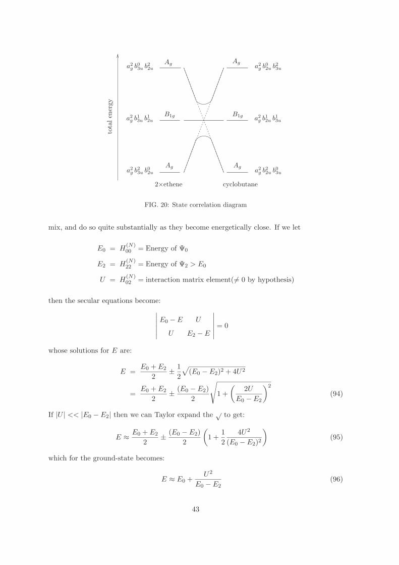
FIG. 20: State correlation diagram

mix, and do so quite substantially as they become energetically close. If we let

E0 = H(N)00 = Energy of Ψ0

E2 = H(N)22 = Energy of Ψ2 > E0

U = H(N)02 = interaction matrix element(6= 0 by hypothesis)

then the secular equations become:

∣∣∣∣∣∣

E0 − E U

U E2 − E

∣∣∣∣∣∣

= 0

whose solutions for E are:

E =E0 + E2

2± 1

2

√

(E0 − E2)2 + 4U2

=E0 + E2

2± (E0 − E2)

2

√

1 +

(2U

E0 − E2

)2

(94)

If |U | << |E0 − E2| then we can Taylor expand the√

to get:

E ≈ E0 + E2

2± (E0 − E2)

2

(

1 +1

2

4U2

(E0 − E2)2

)

(95)

which for the ground-state becomes:

E ≈ E0 +U2

E0 − E2(96)

43

(note E0 − E2 < 0), whilst the doubly-excited state goes as

E ≈ E2 −U2

E0 − E2(97)

In other words, the two states repel each other, irrespective of the sign of U ; the ground-

state is lowered in energy and the excited state pushed up. This is the basis for the non-

crossing rule for states with the same symmetry. The first excited state, being of a different

symmetry, is unaffected. The magnitude of the repulsion depends both on |U | and on the

energy difference denominator, the latter growing as the transition state increases. The effect

of the configuration interaction is most noticeable at transition states.

Nevertheless, even with the above lowering of energy, there remains a large barrier (com-

pared to the thermal energy availble to the molecules) to reaction for the ground-state, and

ethene dimerisation remains thermally forbidden.

The same considerations hold for example in reactions such as H2+I2, long thought to

proceed in a concerted fashion via a rectangular transition state, but in fact shown experi-

mentally to involve iodine atoms. The concerted reaction has a high barrier, which can be

rationalised analogously to the ethene dimerisation problem.

Turning now to the [4+2] cycloaddition, we construct an the orbital correlation diagram,

labelling the MO’s according to their behaviour under σv (Fig. 21).

s

s

s

s

s

sa

a

a

a

a

aEner

gy

FIG. 21: On the LHS, the pπ-based MO’s of the reacting species are labelled symmetric (s) or

antisymmetric (a) under the action of a vertical mirror plane, assuming a symmetrical transition

state. On the RHS, the product, whose MOs now also have σ character in the newly formed bonds,

are similarly labelled.

44

It can be seen that the occupied levels in the reactant and product correlate with each

other, as opposed to the case of the [2+2] dimerisation. In this case, the reaction can proceed

with little barrier, and is therefore thermally accessible.

Similar considerations work for ring opening and closing, see problem 16, where “conro-

tatory” and “disrotatory” mechanisms can be allowed or forbidden, which leads to methods

for selective synthesis of cis or trans products.

XI. AN IMPORTANT FAILURE OF MO THEORY: MOLECULAR DISSOCIATION

Thus far we have dealt with some (great) successes of MO theory, even specialised to

its Huckel form. The impression should not be given, however, that the theory is always

correct, even qualitatively. The principal and ultimate shortcoming of the method comes

from the lack of proper treatment of electron-electron interactions, the latter manifesting

itself in important electron correlation phenomena which no one-electron theory - however

sophisticated - can describe. The aim of this section is to give an account of one of the most

important examples of such failures. Although one could choose examples from hydrocarbon

chemistry, the standard example actually occurs in the simplest of chemical systems, namely

the H2 molecule.

Consider the H2 molecule, whose complete MO wavefunction is written is in terms of the

MO’s of the molecule:

ψ1 =1√2(φ1 + φ2)

ψ2 =1√2(φ1 − φ2) (98)

where φ1 and φ2 refer to the (normalised) 1s orbital on atom 1 and 2 respectively. [Note the

analogy with the ethelene system here. Instead of using pz orbitals, we are using s orbitals.

This, of course, affects the numerical values of the α and β integrals, but does not much

affect the structure of the theory].

These two states are, of course, the 1σg and 1σ∗u bonding and anti-bonding orbitals you

are very familiar with, but we prefer to use the ψi notation to keep things general.

Let us try to construct the total ground-state (electronic) wavefunction for the H2 molecule.

We denote the total wavefunction as Ψ, and note that it will be dependent on the coordinates

45

and spins of two electrons:

Ψ = Ψ(x1,x2) (99)

In what follows, we will refer to Ψ(x1,x2) simply as Ψ(1, 2).

Since both electrons occupy the bonding orbital ψ1, but with opposite spins, we can try

to construct the wavefunction by placing electron 1 in an α spin-state and electron 2 in a β

spin state:

Ψ(1, 2) = ψ1(1)α(1) × ψ1(2)β(2) (100)

You should immediately object to this wavefunction: it does not obey the Pauli principle,

that if we interchange the labels of electron 1 and 2, then the wavefunction should simply

change sign, which it manifestly does not:

Ψ(2, 1) = ψ1(2)α(2) × ψ1(1)β(1) 6= −Ψ(1, 2) (101)

What we have done if to assign electron 2 to spin α, and electron 1 to the spin β. We use

subscripts to denote the spatial orbitals, whilst the labels of individual electrons is placed in

round brackets, eg (1) or (2).

There is a simple recipe to construct anti-symmetric wavefunction, which is to use a

determinant. Let us first begin by constructing the two possible spin-orbitals:

χ1 = ψ1α

χ2 = ψ1β (102)

If electron 1 is inserted in χ1 we get

χ1(1) = ψ1(1)α(1) (103)

and if it is inserted in χ2, we would get:

χ2(1) = ψ1(1)β(1) (104)

Similarly, if we insert electron 2 into χ1 and χ2 respectively, we obtain

χ1(2) = ψ1(2)α(2), χ2(2) = ψ1(2)β(2). (105)

Note that the χi are ortho-normal, e.g.:

〈χ1|χ1〉 = 〈ψ1|ψ1〉〈α|α〉 = 1

〈χ1|χ2〉 = 〈ψ1|ψ1〉〈α|β〉 = 0

46

When you have two-electron bra-kets, you need to take care of the electron labels as well, by

gathering each electron label into its own bra-ket. E.g.

〈χ2(1)χ1(2)|χ1(1)χ2(2)〉 = 〈χ2(1)|χ1(1)〉 × 〈χ1(2)|χ2(2)〉

which in this case equals 0.

Let us construct the following determinant:

Ψ(1, 2) =

∣∣∣∣∣∣

χ1(1) χ2(1)

χ1(2) χ2(2)

∣∣∣∣∣∣

Why does this help? Consider exchanging the labels of the two electrons:

Ψ(2, 1) =

∣∣∣∣∣∣

χ1(2) χ2(2)

χ1(1) χ2(1)

∣∣∣∣∣∣

You can see that this amounts to exchanging two rows of a determinant. Recall that this

operation changes the sign of the the determinant:

Ψ(2, 1) =

∣∣∣∣∣∣

χ1(2) χ2(2)

χ1(1) χ2(1)

∣∣∣∣∣∣

= −

∣∣∣∣∣∣

χ1(1) χ2(1)

χ1(2) χ2(2)

∣∣∣∣∣∣

= −Ψ(1, 2)

Note, also, that if we place both electrons into the same spin-orbital, the determinant vanishes

identically (two columns would be identical). This form of wavefunction, therefore, also

forbids multiple occupation of spin-orbitals (as it should).

This means that we now have, at least, a wavefunction Ψ(1, 2) which is acceptable to

Pauli. Let us expand the determinant:

Ψ(1, 2) = χ1(1)χ2(2) − χ1(2)χ2(1)

Is it normalised? No:

〈Ψ(1, 2)|Ψ(1, 2)〉 = 〈χ1(1)χ2(2) − χ1(2)χ2(1)|χ1(1)χ2(2) − χ1(2)χ2(1)〉

= 〈χ1(1)χ2(2)|χ1(1)χ2(2)〉 − 〈χ1(1)χ2(2)|χ1(2)χ2(1)〉

− 〈χ1(2)χ2(1)|χ1(1)χ2(2)〉 + 〈χ1(2)χ2(1)|χ1(2)χ2(1)〉

Note that:

〈χ1(1)χ2(2)|χ1(2)χ2(1)〉 = 〈χ1(1)|χ2(1)〉 × 〈χ2(2)|χ1(2)〉

= 0

47

whilst

〈χ1(1)χ2(2)|χ1(1)χ2(2)〉 = 1

Therefore we get:

〈Ψ(1, 2)|Ψ(1, 2)〉 = 2

i.e. to get a normalised Ψ(1, 2) we need to divide by√

2:

Ψ(1, 2) =1√2

∣∣∣∣∣∣

χ1(1) χ2(1)

χ1(2) χ2(2)

∣∣∣∣∣∣

(106)

In terms of ψ1 and the spin functions, we have:

Ψ(1, 2) =1√2

ψ1(1)α(1)︸ ︷︷ ︸

χ1(1)

ψ1(2)β(2)︸ ︷︷ ︸

χ2(2)

−ψ1(2)α(2)︸ ︷︷ ︸

χ1(2)

ψ1(1)β(1)︸ ︷︷ ︸

χ2(1)

=ψ1(1)ψ1(2)√

2[α(1)β(2) − β(1)α(2)] (107)

You will immediately recognise this as a singlet (S = 0) state. Given that ψ1 has σ symmetry,

this implies that the corresponding term symbol is 1Σ+g .

Now, what is the difficulty with this wavefunction? Let us expand it now in terms of the

AO’s φ1 and φ2. Since ψ1 = (φ1 + φ2)/√

2, we have:

Ψ(1, 2) =1

(√

2)3[φ1(1) + φ2(1)] [φ1(2) + φ2(2)] [α(1)β(2) − β(1)α(2)]

Expanding the product over the spatial orbitals, we get (omitting the spin wavefunction to

reduce clutter):

Ψ(1, 2) ∼

φ1(1)φ1(2)︸ ︷︷ ︸

ionic

+φ1(1)φ2(2)︸ ︷︷ ︸

biradical

+φ2(1)φ1(2)︸ ︷︷ ︸

biradical

+φ2(1)φ2(2)︸ ︷︷ ︸

ionic

(108)

What is the interpretation of the terms above? The first term puts electron 1 and electron

2 both in AO φ1, i.e. the 1s orbital belonging to one of the nuclei. The 4th term, similarly,

puts both electrons about the second nucleus. The middle two terms place one electron on

one nucleus, and the second electron on the other. One can think of these as the following

chemical entities:

H− H+, H · H·, H+ H−

48

In other words, this wavefunction cannot describe molecular dissociation properly, since it

retains these ionic (i.e. H− H+) components even in that limit. These components have

a high electron-electron repulsion energy. The energy of such a wavefunction is much too

high compared to its exact value (which in thse case of dissociated H2 is 1 Hartree). In the

exact wavefunction, the probablity of finding two electrons around the same nucleus is very

small, compared to that (50%) implied by the MO wavefunction. In other words, in order

to improve the description of molecular dissociation, one must introduce electron correlation,

such that if one electron finds itself around one nucleus, the other electron has an enhanced

probability of finding itself around the other nucleus.

How can one introduce such electron correlation? Let us note that the single-determinant

description of the two-electron wavefunction is itself an approximation. We may be able

to do better by mixing other determinants into the present one, to yield a better overall

wavefunction. Let us denote the above, approximate, wavefunction as Ψ0. Then we would

expect the “exact” wavefunction to be written as

Ψexact(1, 2) = Ψ0(1, 2) +∑

I

cIΨI(1, 2) (109)

where ΨI(1, 2) are determinants constructed out of the unoccupied manifold of MOs, and cI

are coefficients to be determined by the variational principle. This method of introducing

electron correlation is called configuration interaction.

In the present case, we can construct a determinant by doubly-occupying the anti-bonding

orbital ψ2 = (φ1 − φ2)/√

2:

Ψ2(1, 2) =1√2ψ2(1)ψ2(2). [α(1)β(2) − β(1)α(2)]

Substituting for ψ2 we get:

Ψ2(1, 2) ∼ [φ1(1) − φ2(1)][φ1(2) − φ2(2)]

= [φ1(1)φ1(2) − φ1(1)φ2(2) − φ2(1)φ1(2) + φ2(1)φ2(2)]

Notice that in Ψ2, the “ionic” components of the wavefunction come with the opposite sign

to the “bi-radical” parts of the wavefunction.

Therefore, if we subtract Ψ2 from Ψ0, we remove the troublesome ionic factors, leaving

(apart from normalisation factors):

Ψ0 − Ψ2 = [φ1(1)φ2(2) − φ2(1)φ1(2)] [α(1)β(2) − β(1)α(2)] (110)

49

which dissociates correctly. Eq.(110) is the simplest example of a configuration-interaction

wavefunction. The energy of this wavefunction is significantly lower than that of Ψ0 at

dissociation. One can equally ask about the contribution of Ψ2 in the undissociated molecule.

In this case, one needs to solve the secular equation (which arise from the variational principle,

exactly as we did for the Huckel system) owing to mixing of these two states. Let us define

H(N)ij = 〈Ψi|H(N)|Ψj〉

where the H(N) is complete (electronic) Hamiltonian for the system (i.e. the N -electron

Hamiltonian, not the one-electron Hamiltonian we normally deal with). This Hamiltonian

contains explicitly the electron-electron repulsion terms which are either absent (or dealt with

in an approximate way) in the one-electron hamiltonian.

The analysis proceeds almost identically as the state-correlation analysis we performed

for the ethene dimerisation. If we let

E0 = H(N)00 = Energy of Ψ0

E2 = H(N)22 = Energy of Ψ2 > E0

U = H(N)02 = interaction matrix element

then the secular equations become:∣∣∣∣∣∣

E0 − E(CI) U

U E2 − E(CI)

∣∣∣∣∣∣

= 0

whose solutions lead to:

E(CI) =E0 + E2

2± 1

2

√

(E0 − E2)2 + 4U2

i.e. (cf Eqs.(94,95)):

E(CI)0 ≈ E0 +

U2

E0 − E2

and

E(CI)2 ≈ E2 −

U2

E0 − E2

Notice that this result is what we would expect from non-degenerate perturbation theory!

Similarly, you can also show that the component of Ψ2 in ΨCI is ≈ U/(E0 − E2) for small

|U/(E0 − E2)| << 1, i.e. in this limit:

ΨCI0 ≈ Ψ0 +

U

E0 − E2Ψ2

50

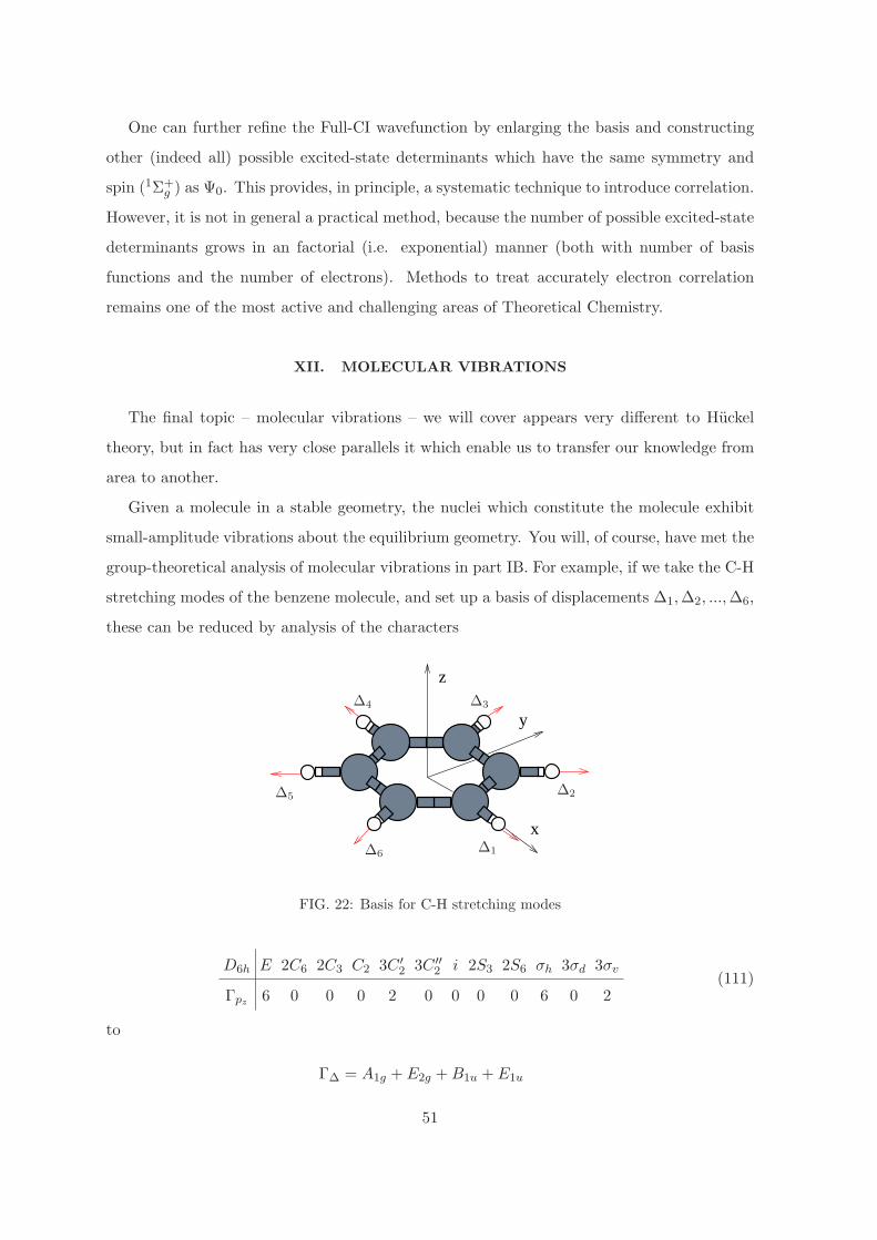
One can further refine the Full-CI wavefunction by enlarging the basis and constructing

other (indeed all) possible excited-state determinants which have the same symmetry and

spin (1Σ+g ) as Ψ0. This provides, in principle, a systematic technique to introduce correlation.

However, it is not in general a practical method, because the number of possible excited-state

determinants grows in an factorial (i.e. exponential) manner (both with number of basis

functions and the number of electrons). Methods to treat accurately electron correlation

remains one of the most active and challenging areas of Theoretical Chemistry.

XII. MOLECULAR VIBRATIONS

The final topic – molecular vibrations – we will cover appears very different to Huckel

theory, but in fact has very close parallels it which enable us to transfer our knowledge from

area to another.

Given a molecule in a stable geometry, the nuclei which constitute the molecule exhibit

small-amplitude vibrations about the equilibrium geometry. You will, of course, have met the

group-theoretical analysis of molecular vibrations in part IB. For example, if we take the C-H

stretching modes of the benzene molecule, and set up a basis of displacements ∆1,∆2, ...,∆6,

these can be reduced by analysis of the characters

x

y

z

∆1

∆2

∆3∆4

∆5

∆6

FIG. 22: Basis for C-H stretching modes

D6h E 2C6 2C3 C2 3C ′2 3C ′′

2 i 2S3 2S6 σh 3σd 3σv

Γpz 6 0 0 0 2 0 0 0 0 6 0 2(111)

to

Γ∆ = A1g + E2g +B1u + E1u

51

you can verify that symmetry-adapted linear combinations of the displacements can be set

up as follows:

QA1g=

1√6

(∆1 + ∆2 + ∆3 + ∆4 + ∆5 + ∆6)

Q(1)E2g

=1

2(∆2 − ∆3 + ∆5 − ∆6)

Q(2)E2g

=1√12

(2∆1 − ∆2 − ∆3 + 2∆4 − ∆5 − ∆6)

Q(1)E1u

=1√12

(2∆1 + ∆2 − ∆3 − 2∆4 − ∆5 + ∆6)

Q(2)E1u

=1

2(∆2 + ∆3 − ∆5 − ∆6)

QB1u=

1√6

(∆1 − ∆2 + ∆3 − ∆4 + ∆5 − ∆6)

These symmetry-adapted displacements can be regarded as approximations to the “normal

modes” of the molecule, which are analogous to the MOs which we obtain by solving Huckel

secular determinants. The question is, for the vibrational problem, what is the analogous

secular determinant, and from where does it arise?

A. Revision of the simple harmonic oscillator

To begin with, let us remind ourselves of the important properties of a one-dimensional

harmonic oscillator. We suppose we have a particle of mass m moving in a potential given

by V (x) = 12kx

2. The Hamiltonian is:

H =1

2mx2 +

1

2kx2

Classically, the particle obeys Newton’s Law, which states that:

mx = −dVdx

giving rise to the familiar equation of motion:

mx = −kx

Solutions to this equation have the form [verify]:

x(t) = A cos(ωt+ φ)

where

ω =

√

k

m(112)

52

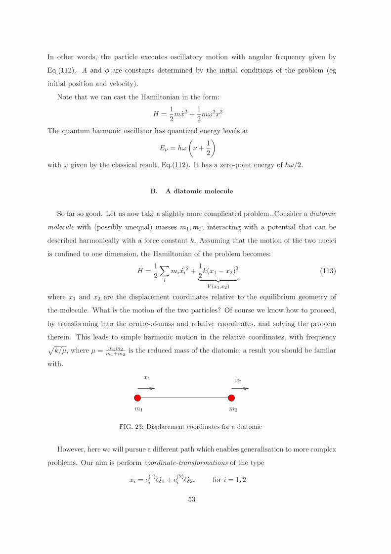
In other words, the particle executes oscillatory motion with angular frequency given by

Eq.(112). A and φ are constants determined by the initial conditions of the problem (eg

initial position and velocity).

Note that we can cast the Hamiltonian in the form:

H =1

2mx2 +

1

2mω2x2

The quantum harmonic oscillator has quantized energy levels at

Eν = hω

(

ν +1

2

)

with ω given by the classical result, Eq.(112). It has a zero-point energy of hω/2.

B. A diatomic molecule

So far so good. Let us now take a slightly more complicated problem. Consider a diatomic

molecule with (possibly unequal) masses m1,m2, interacting with a potential that can be

described harmonically with a force constant k. Assuming that the motion of the two nuclei

is confined to one dimension, the Hamiltonian of the problem becomes:

H =1

2

∑

i

mixi2 +

1

2k(x1 − x2)

2

︸ ︷︷ ︸

V (x1,x2)

(113)

where x1 and x2 are the displacement coordinates relative to the equilibrium geometry of

the molecule. What is the motion of the two particles? Of course we know how to proceed,

by transforming into the centre-of-mass and relative coordinates, and solving the problem

therein. This leads to simple harmonic motion in the relative coordinates, with frequency√

k/µ, where µ = m1m2

m1+m2is the reduced mass of the diatomic, a result you should be familar

with.

x1 x2

m1 m2

FIG. 23: Displacement coordinates for a diatomic

However, here we will pursue a different path which enables generalisation to more complex

problems. Our aim is perform coordinate-transformations of the type

xi = c(1)i Q1 + c

(2)i Q2, for i = 1, 2

53

so as to convert the Hamiltonian Eq.(113) into the form:

H =∑

i

(1

2Qi

2+

1

2ω2

iQ2i

)

(114)

i.e. (in this case two) uncoupled harmonic oscillators in the transformed variables Q1, Q2,

and whose motions are given by:

Qi(t) = Ai cos(ωit+ φi)

where ωi is the corresponding angular frequency for “mode” i. .

The remarkable aspect is that these coordinate transformations turn to be nearly perfectly

analogous to the problem of finding MOs from AOs in Huckel theory!

First, we transform to mass-weighted coordinates:

qi =√mixi (115)

which results in the mass factors being removed from the KE term:

H =1

2

∑

i

qi2 +

1

2k

(q1√m1

− q2√m2

)2

(116)

This can now be cast in the form [verify!]:

H =1

2

∑

i

qi2 +

1

2

∑

ij

qiKijqj (117)

where K is the following matrix:

K =

km1

− k√m1m2

− k√m1m2

km2

(118)

called the dynamical or Hessian matrix.

Since we are looking for uncoupled Hamiltonians of the form Eq.(114), let us suppose that

we have solved for the eigenvectors (and eigenvalues) of the Hessian, i.e. we have in hand the

following:

∑

j

Kijc(n)j = λnc

(n)i (119)

where c(n)i is the i-th component of the n-th (normalised) eigenvector, and λn the correspond-

ing eigenvalue. Recall that such eigenvectors are orthonormal:

∑

i

c(n)i c

(m)i = δnm (120)

54

What use are these eigenvectors? If we let

qi =∑

n

c(n)i Qn (121)

and substitute into the second term of Eq.(117) we obtain:

∑

ij

qiKijqj =∑

ij

[∑

n

c(n)i Qn

]

Kij

[∑

m

c(m)j Qm

]

(122)

Rearranging the sums:

∑

ij

[∑

n

c(n)i Qn

]

Kij

[∑

m

c(m)j Qm

]

=∑

nm

Qn

∑

ij

c(n)i Kijc

(m)j

Qm

=∑

nm

QnλmδnmQm

=∑

n

λnQ2n (123)

In other words, the transformation Eq.(121) casts the terms in precisely the required diagonal

form of Eq.(114), as long as we make the identification:

λn = ω2n (124)

The KE terms are unaffected by the transformation, and remain in diagonal form:

∑

i

q2i =∑

i

[∑

n

c(n)i Qn

][∑

m

c(m)i Qm

]

=∑

nm

Qn

[∑

i

c(n)i c

(m)i

]

Qm

=∑

nm

QnδnmQm

=∑

n

Q2n

In other words, finding the eigenvectors/values of the Hessian matrix completely solves the

problem. Let us therefore proceed with this task for the diatomic system. The secular

equation are:∣∣∣∣∣∣

km1

− λ − k√m1m2

− k√m1m2

km2

− λ

∣∣∣∣∣∣

= 0 (125)

leading to:

(k

m1− λ

)(k

m2− λ

)

− k2

m1m2= 0

55

i.e.

λ2 − λ

(k

m1+

k

m2

)

+k2

m1m2− k2

m1m2= 0

which is solved by:

λ1 = 0,

λ2 =

(k

m1+

k

m2

)

or, if we write:

1

µ=

1

m1+

1

m2

and recall that λn = ω2n (Eq.(124)), we have

ω21 = 0

ω22 =

k

µ

in agreement with our expectations. What do these two frequencies physically relate to? The

eigenvectors c(i) satisfy:

For ω21 = 0 :

1m1

− 1√m1m2

− 1√m1m2

1m2

c(1) = 0 → c(1) =1√M

√m1

√m2

(126)

where M = m1 +m2.

For ω22 =

k

µ:

− 1

m2− 1√

m1m2

− 1√m1m2

− km1

c(2) = 0 → c(2) =1√M

√m2

−√m1

(127)

Writing the modes as :

Qn =∑

i

c(n)i qi (128)

=∑

i

c(n)i

√mixi (129)

we find:

Q1 =1√M

[√m1

√m1x1 +

√m2

√m2x2]

=1√M

[m1x1 +m2x2]

Q2 =1√M

[√m2

√m1x1 −

√m1

√m2x2]

=√µ(x1 − x2)

56

Thus Q1 is proportional to the centre-of-mass coordinate, whilst Q2 corresponds to the rela-

tive coordinate. Varying Q1 shifts the molecule rigidly, whilst varying Q2 gives rise to pure

vibrational motion. Thus we have derived the behaviour of the diatomic without assum-

ing/guessing any knowledge of the likely behaviour. The advantage of this strategy is that it

generalises to polyatomics.

C. Generalisation to polyatomics

Consider a molecule consisting of N nuclei, whose cartesian coordinates are denoted by,

R ≡ {R1,R2, ..,RN} (130)

In 3D space, each particle has 3 cartesian coordinates (x, y, z along a lab-fixed frame) , making

a total of 3N such coordinates. A potential energy function V (R) can be assumed to exist

which gives the potential energy of the molecule as a function of the particle coordinates.

Let us assume the molecule exists in a stable equilbrium geometry, denoted by R(0) =

{R(0)1 ,R

(0)2 , ..,R

(0)N }, about which it performs small-amplitude oscillations. It is convenient

to define any instantaneous position of the nuclei with reference to the equilibrium geometry,

so that

Ri = R(0)i + ∆i (131)

where ∆i refers to the displacement vector of particle i from the equilibrium position. To

make the notation compact in the following few equations, we will refer to the components

of the displacement vectors ∆ as:

{x1, x2, x3︸ ︷︷ ︸

∆1

, x4, x5, x6︸ ︷︷ ︸

∆2

, ..., x3N−2, x3N−1, x3N︸ ︷︷ ︸

∆N

} (132)

In the equilibrium geometry, the forces on the nuclei vanish, and therefore:

(∂V

∂xi

)

0

= 0 (133)

The subscript 0 indicates that the derivative is to be evaluated with all ∆i = 0. Since the

nuclei perform small-amplitude oscillations about this equilibrium position, we can Taylor-

expand the PE as:

V (R) = V0 +1

2

∑

ij

(∂2V

∂xi∂xj

)

0

xixj + cubic terms xixjxk + ... (134)

57

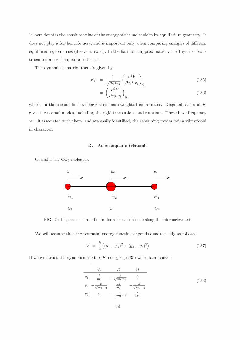
V0 here denotes the absolute value of the energy of the molecule in its equilibrium geometry. It

does not play a further role here, and is important only when comparing energies of different

equilibrium geometries (if several exist). In the harmonic approximation, the Taylor series is

trucanted after the quadratic terms.

The dynamical matrix, then, is given by:

Kij =1

√mimj

(∂2V

∂xi∂xj

)

0

(135)

=

(∂2V

∂qi∂qj

)

0

(136)

where, in the second line, we have used mass-weighted coordinates. Diagonalisation of K

gives the normal modes, including the rigid translations and rotations. These have frequency

ω = 0 associated with them, and are easily identified, the remaining modes being vibrational

in character.

D. An example: a triatomic

Consider the CO2 molecule.

y1 y2 y3

m1m1 m2

O1 O2C

FIG. 24: Displacement coordinates for a linear triatomic along the internuclear axis

We will assume that the potential energy function depends quadratically as follows:

V =k

2

((y1 − y2)

2 + (y2 − y3)2)

(137)

If we construct the dynamical matrix K using Eq.(135) we obtain [show!]:

q1 q2 q3

q1k

m1− k√

m1m20

q2 − k√m1m2

2km2

− k√m1m2

q3 0 − k√m1m2

km1

(138)

58

which bears a close resemblence to the Huckel Hamiltonian of a linear chain. Although it can

be diagonalised directly, we can use symmtery to simplify the problem, a technique which for

larger molecules is indispensible.

Although the point group of CO2 is D∞h, it is more convenient to construct the character

table under a suitable finite subgroup ( e.g. C2v), and then to use “descent-in-symmetry”

tables to identify the irreps of D∞h. We have:

C2v E Cz σxz σyz

Γx1,x32 0 0 2 A1 +B2

Γx21 −1 −1 1 B2

(139)

i.e.

Γall = A1 + 2B2 (140)

We should therefore expect:

A1 : 1 × 1 Hessian

B2 : 2 × 2 Hessian

Group theory tables tell us Γtrans = Γy = B2, and furthermore, descent-in-symmetry

tables tell us the corresponding irreps in D∞h:

A1 → Σ+g

B2 → Σ+u

therefore Γvib = Σ+g + Σ+

u . Let us see how these arise.

First, construct the symmetry-adapted linear combination of the mass-weighted displace-

ments (by inspection, or more formally, using the projection operator as in Huckel theory):

Σ+g : φ1 = (q1 − q3)/

√2 (141)

Σ+u : φ2 = q2 (142)

φ3 = (q1 + q3)/√

2 (143)

The (non-zero) matrix elements of the dynamical matrix in this representation are simply

59

computed. Eg.:

〈φ1|K|φ1〉 =1

2〈q1 − q3|K|q1 − q3〉 =

k

m1

〈φ2|K|φ2〉 = 〈q2|K|q2〉 =2k

m2

〈φ2|K|φ3〉 =1√2〈q2|K|q1 + q3〉 = −

√2k√

m1m2

〈φ3|K|φ3〉 =1

2〈q1 + q3|K|q1 + q3〉 =

k

m1

So the Hessian becomes:

φ1 φ2 φ3

φ1k

m10 0

φ2 0 2km2

−√

2k√m1m2

φ3 0 −√

2k√m1m2

km1

(144)

We immediately get one solution

Σ+g : λ1 =

k

m1(145)

which is purely given by φ1 = 1√2(q1 − q3) =

√m1

2 (x1 − x3); this is the symmetric stretch

with freqency ω1 =√

k/m1.

The other two solutions with Σ+u symmetry are obtained from:

∣∣∣∣∣∣

2km2

− λ −√

2k√m1m2

−√

2k√m1m2

km1

− λ

∣∣∣∣∣∣

= 0

(2k

m2− λ

)(k

m1− λ

)

− 2k2

m1m2= 0

λ2 − λ

(2k

m2+

k

m1

)

= 0

λ =

0

kMm1m2

, (M = 2m1 +m2)(146)

λ = 0 corresponds to the rigid translation of the whole molecule (with ω2 = 0), whilst the

third solution gives the frequency of the anti-symmetric stretch mode, ω3 =√

kM/(m1m2).

The normal modes can also be easily worked out. We do this for the Σ+u anti-symmetric

stretch, which involves finding the appropriate linear combinations of φ2 and φ3. We have

60

ω2 = kM(m1m2) :

2m2

− ω2 −√

2√m1m2

−√

2√m1m2

1m1

− ω2

c(antisym) = 0

2m2

− M(m1m2) −

√2√

m1m2

−√

2√m1m2

1m1

− M(m1m2)

c(antisym) = 0

→ c(antisym) =1√M

−√

2m1

√m2

Q(antisym) =∑

i

c(antisym)i φi

=1√M

(−√

2m1φ2 +√m2φ3

)

=1√M

(

−√

2m1.√m2x2 +

√m2.

√m1

2(x1 + x3)

)

=

õ

2(x1 − 2x2 + x3) ; (µ =

m1m2

M)

The Σ+g symmetric stretch normal mode is left as an exercise.

XIII. QUANTUM THEORY OF MOLECULAR VIBRATIONS AND

VIBRATIONAL SELECTION RULES

The quantum mechanical theory for molecular vibrations proceeds most easily in terms

of the normal-mode coordinates, Qk, which now take on the form of operators. The corre-

sponding momentum operator pk, conjugate to Qk, is pk = ih∂/∂Qk, and in the harmonic

approximation, the Hamiltonian operator is expressible as a sum over uncoupled oscillators:

H =∑

i

(

− h2

2

∂2

∂Q2i

+1

2ω2

iQ2i

)

(147)

The vibrational wavefunction for the entire molecule factorises into a product of harmonic

oscillator states, one for each mode:

Ψν1,ν2...(Q1, Q2...) = ψν1(Q1)ψν2

(Q2)... (148)

(there being 3N − 6 modes for non-linear molecules and 3N − 5 for linear ones). When

we only want to emphasize the occupation numbers of each mode, we will write the total

wavefunction as:

Ψν1,ν2... = |ν1, ν2....〉 (149)

61

In this notation, for example, the state in which there is a single excitation in mode i, all

other modes being empty, is written as |01, 02, ...., 1i, 0i+1...〉.The ψνi

satisfies the Schrodinger equation:

(

− h2

2

∂2

∂Q2i

+1

2ω2

iQ2i

)

ψνi= Eνi

ψνi(150)

with solutions (which you have met in Part IB “Introduction to Quantum Mechanics”) ex-

pressed in terms of a scaled normal coordinate, yi:

yi =

√ωi

hQi (151)

ψνi(yi) = Cνi

Hνi(yi) exp(−y2

i /2) (152)

where Hν is a Hermite polynomial, the first few of which are:

H0(y) = 1 (153)

H1(y) = 2y (154)

H2(y) = 4y2 − 2 (155)

H3(y) = 8y3 − 12y (156)

Cν = (2νν!π1/2)−1/2 is a normalisation factor. The energy of the νth state of the ith mode,

Eνi, is given by:

Eνi= (

1

2+ νi)hωi (157)

and the total energy of Ψν1,ν2... is given by:

H|ν1, ν2...〉 = Eν1,ν2...|ν1, ν2...〉 (158)

Eν1,ν2... =∑

i

(1

2+ νi)hωi (159)

where the sum over i extends over all 3N − 6 (or 3N − 5) normal modes of the molecule.

The vibrational ground-state, denoted by |01, 02, ...〉, with zero quanta in each mode, has the

zero-point energy

E01,02,... =∑

i

hωi/2 (160)

and the ground-state wavefunction has the form:

〈Q1, Q2, ...|01, 02, ...〉 = C exp(−∑

i

ωiQ2i /2h) (161)

62

The symmetry of vibrational wavefunctions can be deduced from the symmetry of the normal

mode. Consider a non-degenerate normal-mode Qi, whose symmetry species is denoted by

Γi. Q2i transforms as the direct product Γi ⊗ Γi = A1 (the fully symmetric representation).

Therefore the symmetry species Γ0iof the ground state ψ0i

∼ exp(−ωiQ2i /2h) is A1, and

more generally, the n-th excited state ψni∼ Qn

i exp(−ωiQi/2h) transforms as Γni= (Γi)

ni .

(The first-excited state goes as Γ1i= Γi, the second as Γ2i

= A1, etc.)

Concerning the total vibrational wavefunction, we can make similar statements. The

ground-state wavefunction given in Eq.(161) contains a sum over squares∑

i ωiQ2i , where

the Qi do now, in general, include degenerate states. Such sums are invariant under any

symmetry operation of the point-group of the molecule. (These operations are orthogonal,

and therefore distance-preserving, transformations). The ground-state, therefore, forms a

basis for the totally symmetric representation A1. More generally, the (excited) state Ψν1,ν2..,,

together with its degenerate partners, form a basis for the (symmetric components of the)

representation of∏

i Γνi

i .

A. Selection rules

These results are particularly useful in deciding whether a mode can be spectroscopically

active, and whether a transition can be stimulated by electromagnetic (EM) radiation. While

the rigorous theory is beyond the scope of this course (we have to deal with the vector

potential associated with the electromagnetic field), we will give a approximate account which

is sufficient for EM radiation of wavelength long compared to molecular dimensions (e.g.

visible light and IR), and which is not very intense. 1 In this case, a molecule placed in an

time varying EM field, whose electric-field vector is given by E(t) = E0 cos(ωt), leads to a

perturbation Hamiltonian of the form:

H(1) = −µ.E(t) (162)

1 There are actually other approximations involved as well: taking into account the first-order in the spatialvariation in the E-field leads to coupling to the quadrupole operator, and to the magnetic-dipole momentoperator, of the system. These terms obey different selection rules to electric-dipole coupling term ofEq.(162), and can induce forbidden transitions. In addition, for a complete theory, one needs to quantizethe EM field, rather than assume it to be classical. This is necessary to account the phenomenon ofspontaneous emission: in the classical theory, an excited state cannot decay into a lower energy statewithout the stimulating presence of an EM field.

63

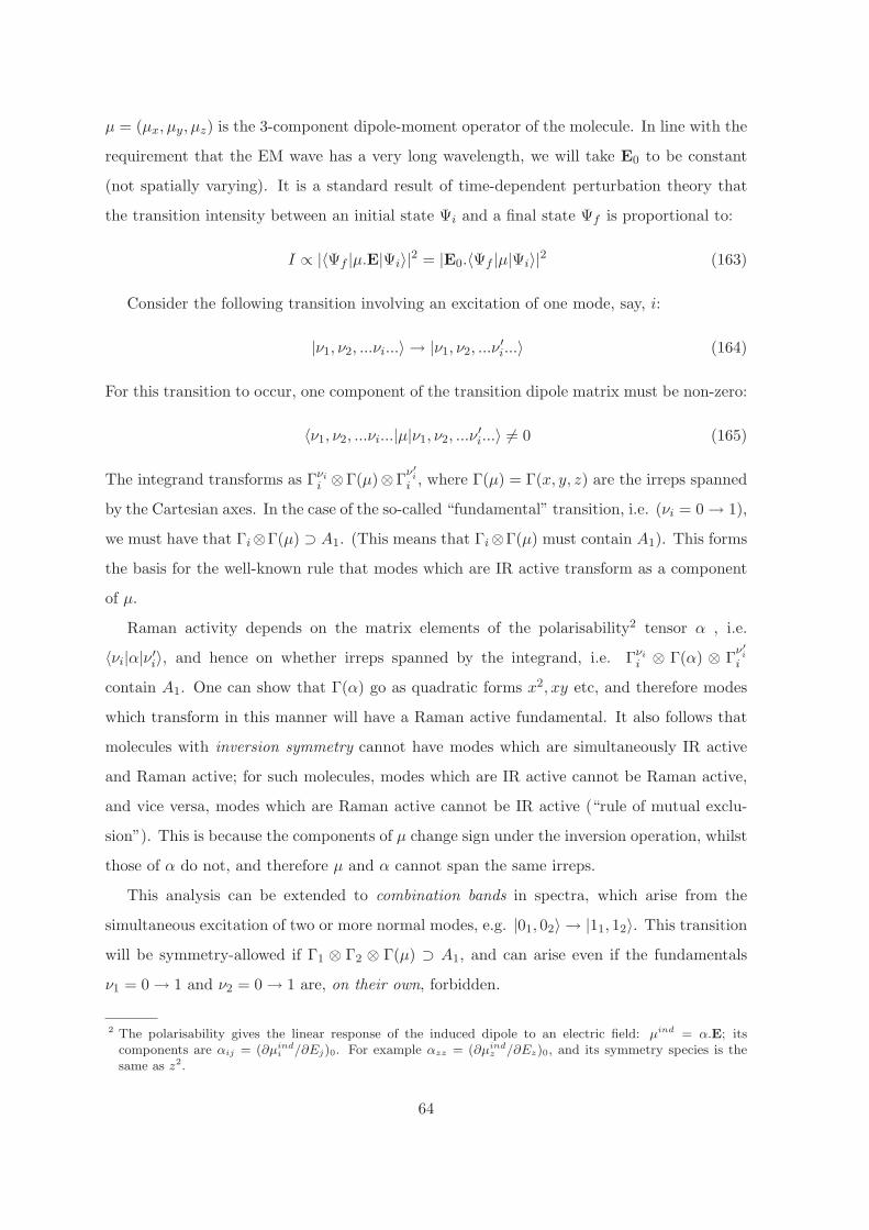
µ = (µx, µy, µz) is the 3-component dipole-moment operator of the molecule. In line with the

requirement that the EM wave has a very long wavelength, we will take E0 to be constant

(not spatially varying). It is a standard result of time-dependent perturbation theory that

the transition intensity between an initial state Ψi and a final state Ψf is proportional to:

I ∝ |〈Ψf |µ.E|Ψi〉|2 = |E0.〈Ψf |µ|Ψi〉|2 (163)

Consider the following transition involving an excitation of one mode, say, i:

|ν1, ν2, ...νi...〉 → |ν1, ν2, ...ν′i...〉 (164)

For this transition to occur, one component of the transition dipole matrix must be non-zero:

〈ν1, ν2, ...νi...|µ|ν1, ν2, ...ν′i...〉 6= 0 (165)

The integrand transforms as Γνi

i ⊗Γ(µ)⊗Γν′

i

i , where Γ(µ) = Γ(x, y, z) are the irreps spanned

by the Cartesian axes. In the case of the so-called “fundamental” transition, i.e. (νi = 0 → 1),

we must have that Γi⊗Γ(µ) ⊃ A1. (This means that Γi⊗Γ(µ) must contain A1). This forms

the basis for the well-known rule that modes which are IR active transform as a component

of µ.

Raman activity depends on the matrix elements of the polarisability2 tensor α , i.e.

〈νi|α|ν ′i〉, and hence on whether irreps spanned by the integrand, i.e. Γνi

i ⊗ Γ(α) ⊗ Γν′

i

i

contain A1. One can show that Γ(α) go as quadratic forms x2, xy etc, and therefore modes

which transform in this manner will have a Raman active fundamental. It also follows that

molecules with inversion symmetry cannot have modes which are simultaneously IR active

and Raman active; for such molecules, modes which are IR active cannot be Raman active,

and vice versa, modes which are Raman active cannot be IR active (“rule of mutual exclu-

sion”). This is because the components of µ change sign under the inversion operation, whilst

those of α do not, and therefore µ and α cannot span the same irreps.

This analysis can be extended to combination bands in spectra, which arise from the

simultaneous excitation of two or more normal modes, e.g. |01, 02〉 → |11, 12〉. This transition

will be symmetry-allowed if Γ1 ⊗ Γ2 ⊗ Γ(µ) ⊃ A1, and can arise even if the fundamentals

ν1 = 0 → 1 and ν2 = 0 → 1 are, on their own, forbidden.

2 The polarisability gives the linear response of the induced dipole to an electric field: µind = α.E; itscomponents are αij = (∂µind

i /∂Ej)0. For example αzz = (∂µindz /∂Ez)0, and its symmetry species is the

same as z2.

64

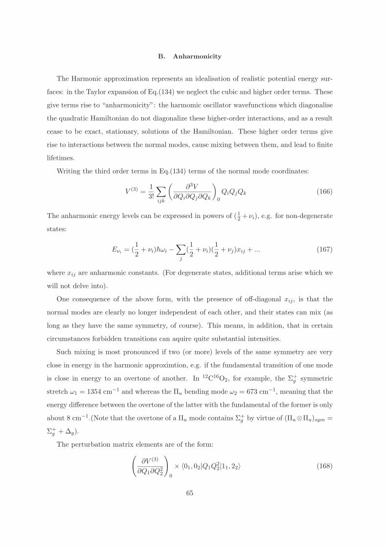
B. Anharmonicity

The Harmonic approximation represents an idealisation of realistic potential energy sur-

faces: in the Taylor expansion of Eq.(134) we neglect the cubic and higher order terms. These

give terms rise to “anharmonicity”: the harmomic oscillator wavefunctions which diagonalise

the quadratic Hamiltonian do not diagonalize these higher-order interactions, and as a result

cease to be exact, stationary, solutions of the Hamiltonian. These higher order terms give

rise to interactions between the normal modes, cause mixing between them, and lead to finite

lifetimes.

Writing the third order terms in Eq.(134) terms of the normal mode coordinates:

V (3) =1

3!

∑

ijk

(∂3V

∂Qi∂Qj∂Qk

)

0

QiQjQk (166)

The anharmonic energy levels can be expressed in powers of (12 + νi), e.g. for non-degenerate

states:

Eνi= (

1

2+ νi)hωi −

∑

j

(1

2+ νi)(

1

2+ νj)xij + ... (167)

where xij are anharmonic constants. (For degenerate states, additional terms arise which we

will not delve into).

One consequence of the above form, with the presence of off-diagonal xij , is that the

normal modes are clearly no longer independent of each other, and their states can mix (as

long as they have the same symmetry, of course). This means, in addition, that in certain

circumstances forbidden transitions can aquire quite substantial intensities.

Such mixing is most pronounced if two (or more) levels of the same symmetry are very

close in energy in the harmonic approximtion, e.g. if the fundamental transition of one mode

is close in energy to an overtone of another. In 12C16O2, for example, the Σ+g symmetric

stretch ω1 = 1354 cm−1 and whereas the Πu bending mode ω2 = 673 cm−1, meaning that the

energy difference between the overtone of the latter with the fundamental of the former is only

about 8 cm−1.(Note that the overtone of a Πu mode contains Σ+g by virtue of (Πu⊗Πu)sym =

Σ+g + ∆g).

The perturbation matrix elements are of the form:

(

∂V (3)

∂Q1∂Q22

)

0

× 〈01, 02|Q1Q22|11, 22〉 (168)

65

and turn out to be significant (∼ 52 cm−1 compared to the 8 cm−1 difference in energy levels).

As a result, the vibrational Raman spectrum shows transitions for both the overtone of the

Πu bending mode and the Σ+g symmetric stretch with similar intensities, whereas the former

would normally be forbidden. This type of mixing between an overtone and a fundamental

which are close in energy is called a “Fermi resonance”.

A final point concerns the behaviour of potential energy surfaces as a function of normal

mode coordinates Qi. In some cases e.g. the symmetric stretch Q1 of the linear triatomic,

the mode is dissociative, which means that V (Q1) tends to an asymptotic constant for large

Q1, corresponding to the energy of the dissociated fragments. Others, such as the bending

mode Q2 and the antisymmetric stretch Q3, are non-dissociative, and the potential energy

increases without bound. This consideration is obviously important if one is trying to model

the potential energy surface, e.g. a Morse potential may be appropriate for the former, but

not for the latter.

66

Problems

Those denoted with ** are quite lengthy problems.

1. (i) Set up and solve without using symmetry the Huckel equations for the π system

of the allyl radical (a) (C3H5), and hence obtain the energy levels and normalised

molecular orbitals. Use diagrams to depict your results.

(ii) Next, using symmetry, write down symmetry-adapted linear combinations of AOs,

and use these to set up the Huckel determinant, and hence solve for the MO’s and

energy levels. Show that you obtain the same result as in (i).

(a) (b)

FIG. 25: (a) Allyl radical, (b) Cyclopropenyl

2. Repeat the above exercise for the cyclopropenyl system, (b).

3. (i) Compute the delocalisation energies of cyclobutadiene and butadiene. Are these

reasonable values? What effects could further stabilise the cyclic molecule?

(ii) Assuming that cyclobutadiene undergoes a distortion to a rectangular geometry, let

us model this by allowing for two different β’s, βs < βl. Using the symmetry-adapted

orbitals, obtain the energy levels for this system, and hence an expression for the total

energy of the distorted molecule. How must the β’s vary for a stabilization to occur?

Does it depend on the value of βl?

4. (For the mathematically inclined). Derive the secular equations, Eq.(14), by finding

stationary values of the ratio, Eq. (6 ), with respect to the MO coefficients cr. [Hint:

consider Eq.(13)].

5. ** In this question, you will use symmetry to solve for the energy levels and MO’s of

naphthalene, shown below.

67

12

3

4

56

7

8

9

10y

x

FIG. 26: Naphthalene, and coordinate system to use.

(i)By grouping the AO’s which transform into each other under the operations of the

point group of the molecule, obtain the irreducible representations spanned by the pπ

orbitals, and determine the number and size of each Huckel determinant which arises.

(ii) Set up the symmetry-adapted orbitals for each irreducible representation.

(iii) Using these, setup the four Huckel secular equations, and solve them to obtain the

energy levels (labelled by the irreducible representations) given below:

B1u : ǫ1 = α+ β(1 +√

13)/2 ≈ α+ 2.30β

B2g : ǫ2 = α+ β(1 +√

5)/2 ≈ α+ 1.62β

B3g : ǫ3 = α− β(1 −√

13)/2 ≈ α+ 1.30β

B1u : ǫ4 = α+ β

Au : ǫ5 = α− β(1 −√

5)/2 ≈ α+ 0.62β

B2g : ǫ6 = α+ β(1 −√

5)/2 ≈ α− 0.62β

B3g : ǫ7 = α− β

B1u : ǫ8 = α+ β(1 −√

13)/2 ≈ α− 1.30β

Au : ǫ9 = α− β(1 +√

5)/2 ≈ α− 1.62β

B3g : ǫ10 = α− β(1 +√

13)/2 ≈ α− 2.30β

Comment on your findings. What is the HOMO-LUMO gap for the neutral molecule?

Compare with the energy levels of the 10-membered cyclic polyene.

(iv) As an optional problem, compute the MO coefficients. Sketch the MOs.

6. Compute the π-populations and bond-orders for the allyl and cyclopropenyl systems

(Ques. 1 and 2), including the radicals, the anions and cations. Comment on what

you find.

68

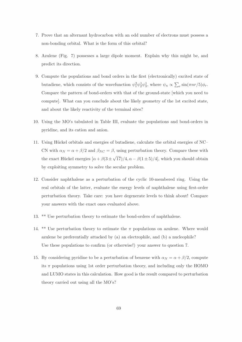
7. Prove that an alternant hydrocarbon with an odd number of electrons must possess a

non-bonding orbital. What is the form of this orbital?

8. Azulene (Fig. 7) possesses a large dipole moment. Explain why this might be, and

predict its direction.

9. Compute the populations and bond orders in the first (electronically) excited state of

butadiene, which consists of the wavefunction ψ21ψ

12ψ

13, where ψn ∝∑r sin(πnr/5)φr.

Compare the pattern of bond-orders with that of the ground-state [which you need to

compute]. What can you conclude about the likely geometry of the 1st excited state,

and about the likely reactivity of the terminal sites?

10. Using the MO’s tabulated in Table III, evaluate the populations and bond-orders in

pyridine, and its cation and anion.

11. Using Huckel orbitals and energies of butadiene, calculate the orbital energies of NC–

CN with αN = α+ β/2 and βNC = β, using perturbation theory. Compare these with

the exact Huckel energies [α+ β(3±√

17)/4, α− β(1± 5)/4], which you should obtain

by exploiting symmetry to solve the secular problem.

12. Consider naphthalene as a perturbation of the cyclic 10-membered ring. Using the

real orbitals of the latter, evaluate the energy levels of naphthalene using first-order

perturbation theory. Take care: you have degenerate levels to think about! Compare

your answers with the exact ones evaluated above.

13. ** Use perturbation theory to estimate the bond-orders of naphthalene.

14. ** Use perturbation theory to estimate the π populations on azulene. Where would

azulene be preferentially attacked by (a) an electrophile, and (b) a nucleophile?

Use these populations to confirm (or otherwise!) your answer to question 7.

15. By considering pyridine to be a perturbation of benzene with αN = α+ β/2, compute

its π populations using 1st order perturbation theory, and including only the HOMO

and LUMO states in this calculation. How good is the result compared to perturbation

theory carried out using all the MO’s?

69

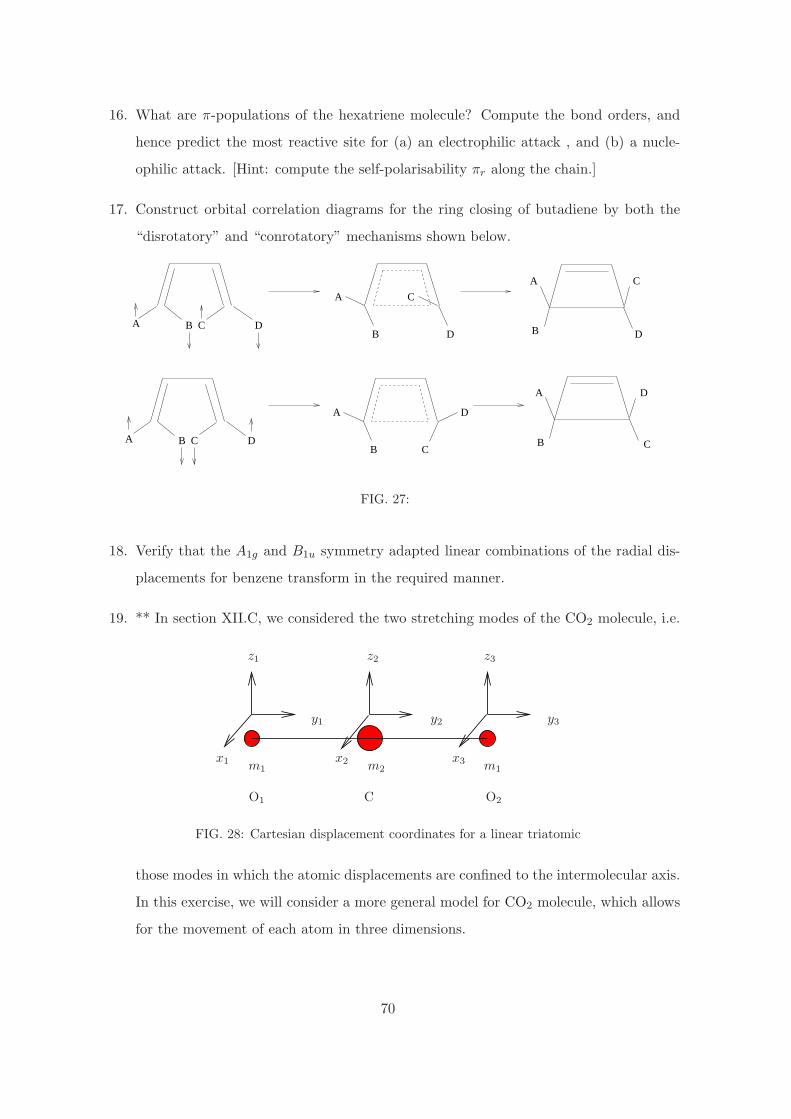
16. What are π-populations of the hexatriene molecule? Compute the bond orders, and

hence predict the most reactive site for (a) an electrophilic attack , and (b) a nucle-

ophilic attack. [Hint: compute the self-polarisability πr along the chain.]

17. Construct orbital correlation diagrams for the ring closing of butadiene by both the

“disrotatory” and “conrotatory” mechanisms shown below.

A B C D

A B C D

A

B

C

D

A

B

C

D

A

B

A

B C

D

C

D

FIG. 27:

18. Verify that the A1g and B1u symmetry adapted linear combinations of the radial dis-

placements for benzene transform in the required manner.

19. ** In section XII.C, we considered the two stretching modes of the CO2 molecule, i.e.

x1

y1

z1

x2

y2

z2

x3

y3

z3

m1m1 m2

O1 O2C

FIG. 28: Cartesian displacement coordinates for a linear triatomic

those modes in which the atomic displacements are confined to the intermolecular axis.

In this exercise, we will consider a more general model for CO2 molecule, which allows

for the movement of each atom in three dimensions.

70

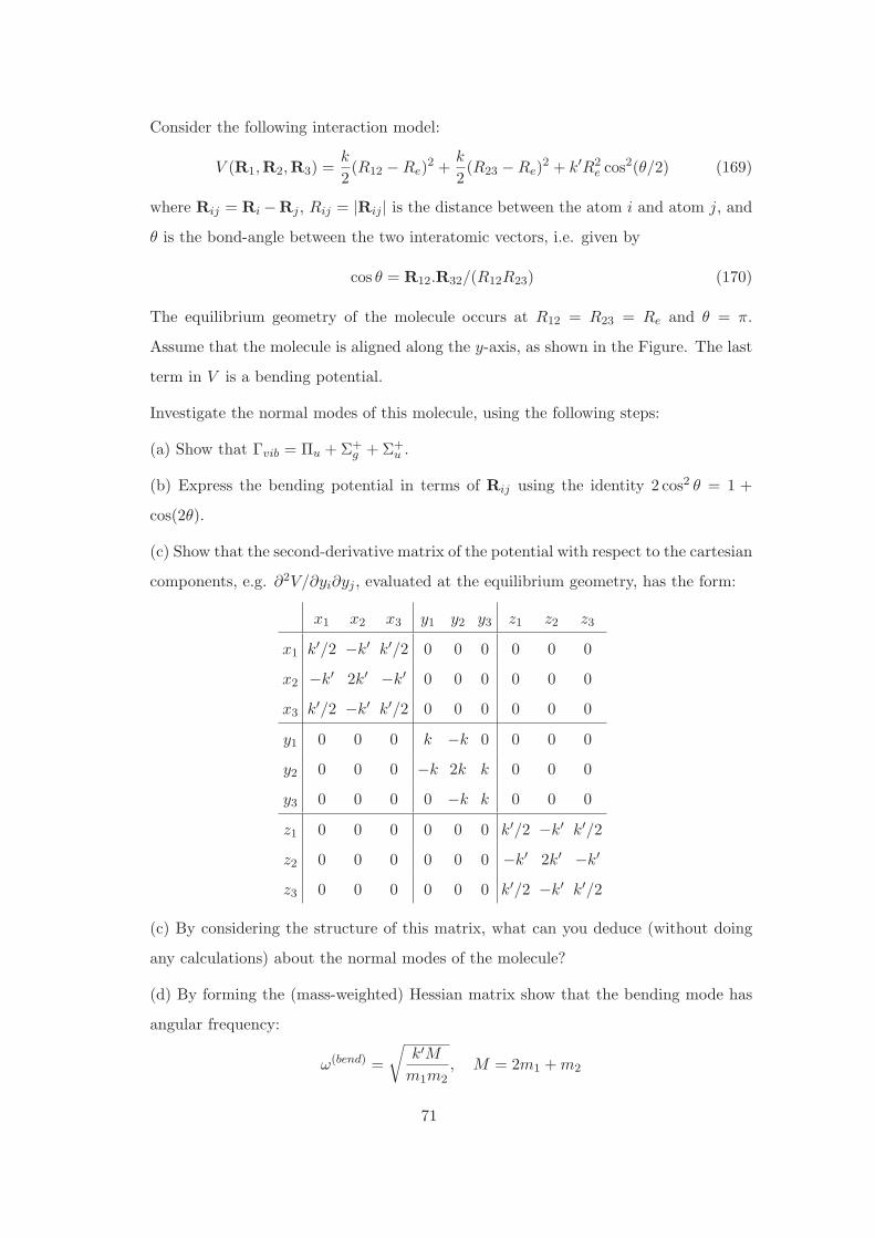
Consider the following interaction model:

V (R1,R2,R3) =k

2(R12 −Re)

2 +k

2(R23 −Re)

2 + k′R2e cos2(θ/2) (169)

where Rij = Ri −Rj , Rij = |Rij | is the distance between the atom i and atom j, and

θ is the bond-angle between the two interatomic vectors, i.e. given by

cos θ = R12.R32/(R12R23) (170)

The equilibrium geometry of the molecule occurs at R12 = R23 = Re and θ = π.

Assume that the molecule is aligned along the y-axis, as shown in the Figure. The last

term in V is a bending potential.

Investigate the normal modes of this molecule, using the following steps:

(a) Show that Γvib = Πu + Σ+g + Σ+

u .

(b) Express the bending potential in terms of Rij using the identity 2 cos2 θ = 1 +

cos(2θ).

(c) Show that the second-derivative matrix of the potential with respect to the cartesian

components, e.g. ∂2V/∂yi∂yj , evaluated at the equilibrium geometry, has the form:

x1 x2 x3 y1 y2 y3 z1 z2 z3

x1 k′/2 −k′ k′/2 0 0 0 0 0 0

x2 −k′ 2k′ −k′ 0 0 0 0 0 0

x3 k′/2 −k′ k′/2 0 0 0 0 0 0

y1 0 0 0 k −k 0 0 0 0

y2 0 0 0 −k 2k k 0 0 0

y3 0 0 0 0 −k k 0 0 0

z1 0 0 0 0 0 0 k′/2 −k′ k′/2z2 0 0 0 0 0 0 −k′ 2k′ −k′

z3 0 0 0 0 0 0 k′/2 −k′ k′/2

(c) By considering the structure of this matrix, what can you deduce (without doing

any calculations) about the normal modes of the molecule?

(d) By forming the (mass-weighted) Hessian matrix show that the bending mode has

angular frequency:

ω(bend) =

√

k′M

m1m2, M = 2m1 +m2

71

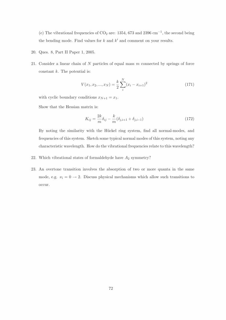
(e) The vibrational frequencies of CO2 are: 1354, 673 and 2396 cm−1, the second being

the bending mode. Find values for k and k′ and comment on your results.

20. Ques. 8, Part II Paper 1, 2005.

21. Consider a linear chain of N particles of equal mass m connected by springs of force

constant k. The potential is:

V (x1, x2, ..., xN ) =k

2

N∑

i

(xi − xi+1)2 (171)

with cyclic boundary conditions xN+1 = x1.

Show that the Hessian matrix is:

Kij =2k

mδij −

k

m(δj,i+1 + δj,i−1) (172)

By noting the similarity with the Huckel ring system, find all normal-modes, and

frequencies of this system. Sketch some typical normal modes of this system, noting any

characteristic wavelength. How do the vibrational frequencies relate to this wavelength?

22. Which vibrational states of formaldehyde have A2 symmetry?

23. An overtone transition involves the absorption of two or more quanta in the same

mode, e.g. νi = 0 → 2. Discuss physical mechanisms which allow such transitions to

occur.

72