A Workflow for Characterizing NanoparticleMonolayers for Biosensors: MachineLearning on Real and Artificial SEM ImagesAdam Hughes1, Zhaowen Liu2, Mayam Raftari3, and M. E. Reeves4

1-4The George Washington University, USA

ABSTRACT

A persistent challenge in materials science is the characterization of a large ensemble of heterogeneousnanostructures in a set of images. This often leads to practices such as manual particle counting, andsampling bias of a favorable region of the “best” image. Herein, we present the open-source software,imaging criteria and workflow necessary to fully characterize an ensemble of SEM nanoparticle images.Such characterization is critical to nanoparticle biosensors, whose performance and characteristicsare determined by the distribution of the underlying nanoparticle film. We utilize novel artificial SEMimages to objectively compare commonly-found image processing methods through each stage of theworkflow: acquistion, preprocessing, segmentation, labeling and object classification. Using the semi-supervised machine learning application, Ilastik, we demonstrate the decomposition of a nanoparticleimage into particle subtypes relevant to our application: singles, dimers, flat aggregates and piles. Weoutline a workflow for characterizing and classifying nanoscale features on low-magnification imageswith thousands of nanoparticles. This work is accompanied by a repository of supplementary materials,including videos, a bank of real and artificial SEM images, and ten IPython Notebook tutorials to reproduceand extend the presented results.

Keywords: Image Processing, Gold Nanoparticles, Biosensor, Plasmonics, Electron Microscopy,Microsopy, Ilastik, Segmentation, Bioengineering, Reproducible Research, IPython Notebook

1 INTRODUCTIONMetallic colloids, especially gold nanoparticles (AuNPs) continue to be of high interdisciplinary in-terest, ranging in application from biosensing(Sai et al., 2009)(Nath and Chilkoti, 2002) to photo-voltaics(Shahin et al., 2012), even to heating water(McKenna, 2012). The optical properties of nanopar-ticles are highly sensitive to their morphology. In sensing applications, nanorods(Becker et al., 2010)and nanoshells(Kessentini and Barchiesi, 2012) show demonstrable enhancement over their sphericalcounterparts; even the AuNP dimer exhibits a central “hot spot”(Cheng et al., 2011). In addition toindividual particle morphology, ensemble properties also drastically affect the response of a nanosystem.While nanofilm sensors exhibit an optimal monolayer fill fraction at which sensitivity peaks(Shahinet al., 2012)(Jeong et al., 2011)(Moirangthem et al., 2011), they are also susceptible to degradationthrough film contamination and aggregation. Since nanoparticle aggregation processes are difficult tocontrol(Kim et al., 2008)(Pease et al., 2010), one must experimentally characterize a nanosystem to ensurequality and consistency between samples. While there are several approaches, including spectral meth-ods(Lopatynskyi et al., 2011)(Khlebtsov, 2008), small-angle X-ray scattering(Gleber et al., 2010), anddynamic light scattering(Jans et al., 2009)(Khlebtsov and Khlebtsov, 2011)1, high-resolution microscopy(HRM) is still the most direct way to obtain detailed nanoscale structural information.

In this context, quantitation of SEM data can be painstaking, with simple approach involving hand-counting of the particles in a typical image(Sciacca and Monro, 2014). Advances in image analysishave enabled the automatic counting and sizing of particles in high contrast images such as transmissionelectron micrographs(Reetz et al., 2000) utilizing prewritten routines in software packages such asMATLABTM (MathWorks, 2013) or Fiji(Schindelin et al., 2012). In biomedical applications, image

1For an excellent comparison of AuNP measurements methods, see Ref. (Meli et al., 2012).

PeerJ PrePrints | http://dx.doi.org/10.7287/peerj.preprints.671v2 | CC-BY 4.0 Open Access | rec: 8 Dec 2014, publ: 8 Dec 2014

PrePrin

ts

analysis from in-house algorithms has been used to classify relevant features in mesoporous silicon forprotein delivery (Alexander et al., 2009). In direct relation to particle identification from SEM images,hybrid approaches combining MATLAB routines and custom code have been used to successfully segmentnanoparticles images(Singh, 2013).

Despite advances in HRM and image processing, it remains challenging to rigorously and consistentlymeasure and classify nanoscale features in an image which itself is many thousands of times larger. Thedomain knowledge interrelating microscopy, nanotechnology and image processing is broad, and imageprocessing guides are often very general(Sankur and Lent, 2004), or focused primarily on biology(Acuntoand Salvetti, 2010)(Eliceiri et al., 2012) and medicine(Lehmann, 1999). Herein, we present a modernworkflow for nanoparticle image processing based on recent advances in open-source software. Wefirst compare several image preprocessing and segmentation techniques based on their performanceon both real and novel artificial SEM images, then demonstrate how to classify different types ofnanoparticles in the same image using the machine-learning application, Ilastik(Sommer et al., 2011).From acquisition to classification, we identify which image processing techniques are the most usefulfor AuNP characterization. These techniques combined into a single workflow are used to automaticallyidentify tens of thousands of nanoparticles in low-magnification images, group them by species, andeliminate the need for manual counting and biased sampling.

The manuscript is outlined as follows: Section 2 describes best-practices in sample preparation andscanning electron microscope (SEM) imaging of AuNP films, followed by an overview of open-sourceimage processing software. We then present novel artificial SEM images, subsequently used in Section 3to objectively quantify and compare segmentation and classification tools. Section 3 first describes caveatsand best practices for SEM imaging, and follows with a comparative survey of segmentation techniques,including thresholding, edge-based, seeded and semi-supervised learning approaches. Following adiscussion on preprocessing, we utilized machine learning applications to classify single particles, dimersand aggregates in both real and artificial SEM images. Section 4 discusses image processing workflows andthe role of image processing in HRM techniques other than SEM. For training and dissemination(Editorial,2014)(Mascarelli, 2014), all results and analysis are available as supplemental IPython(Perez and Granger,2007) Notebook tutorials(Hughes, 2014a), enumerated in Table 1 and henceforth referred to simply asNotebooks.

2 MATERIALS AND METHODS

2.1 Sample PreparationCitrate-capped gold nanoparticles (AuNPs) of mean diameter 21nm were synthesized according to thestandard reduction protocol(Turkevich et al., 1951). Size distributions were ascertained through carefulcentroid-centroid distance measurements of dimer particles in TEM and SEM images; complimentary sizeand concentration data were obtained through empirical spectroscopic approaches(Khlebtsov, 2008)(Haisset al., 2007)(Amendola and Meneghetti, 2009). AuNPs were deposited onto amino-functionalized opticalfibers [GIF-625 Thorlabs] using a protocol similar to Ref. (Shahin et al., 2012). Prior to imaging, fiberswere immersed in ethanol to remove contaminants like those found in Fig. (1b), which absorb quicklyonto the highly-charged, functionalized glass.

2.2 SoftwareThere are numerous software tools for image processing(Eliceiri et al., 2012). Popular open-sourcelibraries include Fiji, scikit-image(van der Walt et al., 2014) and Octave(Kovesi, 2000), while commercialsolutions in MATLABTM and MathematicaTM are also available. Fiji is a distribution of the highly successfulImageJ(Schneider, C.A., Rasband, W.S., Eliceiri, 2012) platform with an impressive suite of pluginsgeared towards biology and microscopy, such as MOSAIC(Sbalzarini and Kournoutsakos, 2005) forparticle tracking, and Weka(Arganda-Carreras, I., Cardona, A., Kaynig, V., Schindelin, 2011) for trainablesegmentation. Scikit-image is a functional library that boasts an elegant API and integration with thescientific Python(Peterson, 2001) stack. Mahotas(Coelho, 2013), another Python imaging library, hasbeen recently employed in the analysis of SEM images of block copolymer nanocomposites(Ploshniket al., 2013). Fiji and scikit-image were used predominately the results presented here; a related li-brary, pyparty(Hughes, 2014c), assisted in artificial image generation and particle analysis. Supervisedsegmentation was performed in Ilastik.

2/19

PeerJ PrePrints | http://dx.doi.org/10.7287/peerj.preprints.671v2 | CC-BY 4.0 Open Access | rec: 8 Dec 2014, publ: 8 Dec 2014

PrePrin

ts

(a) (b)

Figure 1. Clean vs. contaminated AuNP films. Typical 22nm monolayer of AuNPs at 100000X (a), and30000X monolayer with microbial contamination (b). Several examples of other commonly observedsurface contaminants and defects are available in supplemental data. One can see examples of smallAuNP aggregates forming.

2.3 Test and Sample ImagesTo compare image processing methods objectively, three high-resolution (3072 x 2304) artificial SEMimages were created. The benefit of using artificial images is the exact particle brightness and sizes areknown apriori, so segmentation errors can be quantified to the pixel. Each image consists of circles ofnominal diameter 30 pixels (σ = 3) arranged into singles (50%), dimers (25%), trimers (12.5%) andtetramers (12.5%) of varying particle size and orientation. 1170 non-overlapping2 particles were overlaidonto a mesh of periodically varying brightness ranging from 80-170, resulting in a surface coverage of21.4%. The particle brightness ranges from 190 to 250 based on a scaled beta-distribution, β (a=2, b=2),slightly biased towards brighter clusters. Brightness variation was chosen to reflect observed distributionsin actual samples. Brightness in this context refers to the monochromatic pixel intensity range between 0and 255.

Fig. (2) shows the three test images, referred to as RASTER, SMOOTH and NOISY, and will be referredto in this special font throughout. RASTER depicts particles with sharp, distinct boundaries. The SMOOTHtest image applies a Gaussian filter (σ = 3px) to RASTER, resulting in blended, realistic boundaries. TheNOISY test image is the SMOOTH image with Gaussian noise added to 25% coverage. In practice, actualelectron microscope noise may not be normally distributed(Nemota, 2012). Notebook 1 is provided togenerate artificial SEM or TEM images.

Twelve real SEM images ranging in magnification from 30-100kX are included in the supplementaldata. These include ideal and flawed images with defects of low and varying contrast, non-circularparticles due to astigmatism, striations from detector discharge(JEOL, 2014) and noise. The real SEMimages are utilized primarily for comparing thresholding methods in the next section, and are availablefor download in the supplemental data.

3 RESULTS

It is difficult to generalize the workflow of image processing,3 as the optimal approach is often reached aftercycles of trial and error. Most often, the final workflow involves 5 steps: Acquisition→ Preprocessing→ Segmentation→ Labeling→Measurement and Object Classification. In the context of AuNPs,this corresponds to first obtaining a suitable image, then separating the particles from background(segmentation), followed by labeling and grouping the particle subtypes (classification), and finally

2Intra-cluster overlap was allowed and ranged to about 20%, for example in tetramers, but overlap between trimer A and dimerB was avoided.

3Woods presents image processing in 11 chapters(Woods, 2002), but notes that segmentation and enhancement are not necessarilyseparate. In addition, some segmentation algorithms incorporate preprocessing; for example, the Canny filter uses Gaussiansmoothing.

3/19

PeerJ PrePrints | http://dx.doi.org/10.7287/peerj.preprints.671v2 | CC-BY 4.0 Open Access | rec: 8 Dec 2014, publ: 8 Dec 2014

PrePrin

ts

Notebook Description1 Generating Test Images2 Measuring Digitization Errors in Small Particles3 Quantifying Segmentation in Binary Images4 Thresholding, Edge, and Seeded Segmentation5 Denoising and Filtering6 Contrast Enhancement7 Intro to Particle Classification8 Segmentation Error in Ilastik9 Classifying Nanoparticles: Ilastik vs. User Partitioning10 Fourier Filtering of the Noisy Test Image

Table 1. Hyperlinks to supplemental IPython Notebooks.

Figure 2. Three artificial test images referred to as RASTER, SMOOTH and NOISY. Top: Cropped (512 x512) region of each image. Left: Color-coded particle species and artificially colored smoothed edges.Bottom right: Brightness histogram decomposed by source, shown from 80 to 255 pixels. The noise andsmoothing effectively mix the background and particle populations which makes segmentation morechallenging on these images. The color scheme of red, green, yellow and magenta will be usedconsistently to refer to singles, dimers, trimers and tetramer particle types, respectively.

producing distributions based on size, shape, brightness and other object features (measurement). Each ofthe subsequent sections corresponds to one of these steps4, with segmentation and object classificationreceiving the most attention. We deviate from the step order by discussing segmentation prior topreprocessing, since shortcomings in the segmentation naturally motivate a discussion of noise removaland contrast enhancement, two important preprocessing techniques.

4Labeling is not discussed in detail because particle labeling routines (connected-component algorithms) are easy accessed, andgive mostly identical across image processing libraries.

4/19

PeerJ PrePrints | http://dx.doi.org/10.7287/peerj.preprints.671v2 | CC-BY 4.0 Open Access | rec: 8 Dec 2014, publ: 8 Dec 2014

PrePrin

ts

3.1 AcquisitionImages (3072 x 2304) were acquired using a ZeissTM EVO LS 25 SEM using the SE2 detector5 at 1kVover a range of magnifications. Nominal line integration and scan average settings resulted in roughlya three minute acquisition time. The SEM chamber vacuum was pumped for at least an hour beforeimaging; and the working distance was 5.5mm. AuNPs of diameter under 20nm in diameter may provedifficult to image reliably, due to their low contrast and distinct halo, which has been previously discussedfrom a theoretical standpoint(Klein et al., 2011). In such cases, we obtained sharper edges using anannular secondary electron detector, but at the cost of higher sensitivity to charging. While the theoreticalresolution of a 1kV beam is about half of the wavelength, or .02nm(Barlow, 2004); the pragmatic valuefor low-voltage is still about 2nm(Microscopy, 2014). Improvements in optics and detectors are narrowingthis gap by overcoming issues related to beam widening,6 chromatic aberration, and insufficient escapevolume of the signal carriers(Amako et al., 2002)(Dellby et al., 2001). For a comprehensive evaluationof SEM imaging aberrations and their causes, consult Ref. (JEOL, 2014). Of those we encountered,charging, astigmatism, and detector discharging were the most difficult to correct for, as they induceparticle warping and local contrast variations simultaneously.

While it is advantageous to image at a large field of view, this lowers particle resolution and leadsto at least two types of digitization errors. The first type is intrinsic to measuring digitized particles(i.e. squaring the circle), and is described in more detail in Section 3.5. The second type is related tothe particle size distribution (i.e. size histogram). At low magnification, the particles are too pixelated,resulting in sparse binning. This is illustrated in Fig. (3), which shows the particle area distributions of thesame sample, imaged at 5000X and 30000X. The measured mean, variance and other important statisticalparameters are no longer reliable. We observed that suitable particles distributions were obtained whenthe object of interest is at least 10 pixels across. Ergo, for 22nm diameter AuNPs, the magnification andresolution settings should result in a scale no larger than 2.2 nm per pixel. At such a scale, just under15000 non-overlapping 22nm diameter AuNPs could fit in a 3072 x 2304 resolution image, covering asurface area of 34um2. Images can be regenerated or modified using notebook 1.

Figure 3. The effect of a 6-fold magnification change on the particle area distribution in same sample.The profile of the distribution is lost at low resolution.

3.2 SegmentationTo group the many approaches to segmentation(Narkhede, 2013), we’ve chosen the following catego-rization: thresholding refers to the segmentation algorithms that primarily analyze pixel brightness.Edge-based segmentation operates on object boundaries, related to the image gradient or Laplacian.Morphological watershedding(Beucher, S ; Lantuejoul, 1979) and random walk segmentation(Grady,2006) have been paired due to phenomenological similarities. Such approaches treat the image as atopographic barrier; in watershedding the analogue is to water basins, in random walks to a diffusion

5The SE2 is an Everhart-Thornley detector that collects a combination of secondary and back-scattered electrons to give bothcompositional and topographical resolution, respectively.

6The repulsion between low-energy electrons make them difficult to focus into a narrow beam.

5/19

PeerJ PrePrints | http://dx.doi.org/10.7287/peerj.preprints.671v2 | CC-BY 4.0 Open Access | rec: 8 Dec 2014, publ: 8 Dec 2014

PrePrin

ts

barrier, and both approaches require user-provided seeds.7 These segmentation algorithms representa broad sampling of various segmentation methodologies; they are straightforward to implement inscikit-image and/or Fiji, and they provide a natural segue into the topic of semi-supervised segmentation.Our overview of segmentation is non-exhaustive. Some popular methods we did not examine includeunsupervised clustering(Tan et al., 2013),various region-based techniques and several graph methods suchas normalized cuts(Malik, 2000).

We assessed performance based on accuracy in segmenting the artificial images. Since the exact parti-cle extents in the test images are known apriori, segmentation performance can be evaluated objectively.Overthresholding and understhresholding are quantified as the false positives (fp), negatives (fn) and net(fp + fn) of the pixels in the segmented image (Γ1) as compared to the binary version of the RASTERtest image (Γ2). Since the binarized images are boolean arrays, this is equivalent to the set intersection(Γ1∩Γ2), as demonstrated in Notebook 3. Because the comparison is to the rastered particles, and not thesmoothed particles, we expect the majority of segmentation methods to overestimate the boundary size.

3.2.1 ThresholdingFiji is distributed with an auto-thresholding plugin(Landini, 2013) that can simultaneously apply 25segmentation algorithms on a single image. Of these, 16 segment based on information in the overall, orglobal, image brightness, while the remaining 9 parse local brightness information to segment subregionsof the image separately. We ranked the 25 algorithms based on their performance on real SEM images,and selected only the top performing methods for further comparison on the artificial images. Acollage summarizing these results is available in the supplemental material. In short, we found that mostof Fiji’s global auto-thresholding routines failed in the presence of the contrast gradients found in realAuNP SEM images. A global brightness cutoff; that is, setting a brightness value and screening all pixelsbelow it, performed well within a narrow cutoff range.

In regard to the 9 local auto-thresholding algorithms, Otsu(Otsu, 1975) performed the best on thereal SEM images, followed by the Bersen and MidGrey methods. Additionally, scikit-image’s Gaussianadaptive threshold function performed reasonably well on some of the sample SEM images.8 Therefore,we chose a global pixel cutoff, Gaussian adaptive thresholding and local Otsu thresholding as threemethods for further evaluation on the artificial test images.

Both adaptive and Otsu thresholding performed poorly on all three of the test images, as they werehighly sensitive to noise, as well as local contrast variations in the background gradient as illustrated inFig. (4). A global brightness cutoff segmented the test images quite well, when set at or near the optimalcutoff value. For the noisy test image, the optimal threshold value is 187 grayscale, reaching only 7.4%net error as shown in Fig. (5). Unfortunately, finding the optimal threshold often requires manual tuning,limiting its utility in batch processing; although we acknowledge that automated approaches to locatingthe optimal global threshold based on summing weighted normal distributions have been proposed(Woods,2002)(Dickerson, 2001). It is important to recognize that the test images were designed such that thedimmest particle is still brighter than the brightest region of the background. Thus, the artificial imagesfavor the global cutoff method by design. In reality, local electronic variations in SEM images blur theglobal separation of background and particles, rendering them impossible to threshold via global cutoff.

3.2.2 Edge-based segmentationIt is often useful to work with the gradient or Lapacian of an image, rather than the image itself. Thegradient emphasizes regions of rapid brightness changes, such as the border between nanoparticle edgesand image background. Edge segmentation techniques are well developed in commercial and open accesspackages, and are well-suited to resolve surface features in SEM images(Midoh et al., 2007). Sincenanoparticles are nonporous, if their outlines can be accurately identified, then segmentation followsmerely from filling in the bound regions. Since it is straightforward to fill an enclosed region of a binaryimage with the standard morphological operations(Cressie and Serra, 1988) found in scikit image, thesuccessfulness of this approach depends on how accurately the particle boundaries can be identified.We chose the Sobel(Sobel and Feldman, 1968) and Canny(Canny, 1986) filters as candidates for edgedetection on the three test images.

7While watershedding without user-specified seeds is possible, it tends to result in oversegmentation(Woods, 2002).8scikit-image’s adaptive thresholding “method” parameter (Gaussian, mean, median etc...) specifies how the threshold value is

determined from the local pixel neighbourhood. Gaussian provided the best results for our images.

6/19

PeerJ PrePrints | http://dx.doi.org/10.7287/peerj.preprints.671v2 | CC-BY 4.0 Open Access | rec: 8 Dec 2014, publ: 8 Dec 2014

PrePrin

ts

Figure 4. Three thresholding methods applied to the RASTER, SMOOTH and NOISY test images. Row1: Cutting out all pixels below a brightness of 150 leads to significant over-thresholding. Row 2: Anoptimal cutoff of 187 gives lowest segmentation error achievable when applying the global cutoff methodto the NOISY image: about 7.4% error as shown in Fig. (5a). Rows 3/4: Gaussian adaptive thresholdingand local Otsu thresholding both fail in the presence of the complex background and noise.

(a) (b)

Figure 5. Comparing segmentation error on NOISY between the global cutoff, watershed and randomwalk methods: (a) Pixel false positives and negatives for a global brightness cutoff shows minimalsegmentation error of 7.4% at brightness 187. (b) Segmentation error for random walk and watershedmethods as a function of seed marker fraction.

The Canny filter is a widely-used edge-detection technique, known for its sensitivity to weak edges androbustness to noise. Canny works by first smoothing an image, then tracing edges based on the strengthof the image gradient(Green, 2002). Canny employs a hysteresis filter to remove small unconnectedfragments, or “streaks”, and retain real edges(Ding and Goshtasby, 2001). The Sobel operator does notfind edges directly; it computes the gradient of the image, and then one must apply a cutoff (masking) to

7/19

PeerJ PrePrints | http://dx.doi.org/10.7287/peerj.preprints.671v2 | CC-BY 4.0 Open Access | rec: 8 Dec 2014, publ: 8 Dec 2014

PrePrin

ts

retain the strongest gradients, which in the case of nanoparticles occur at the particle edges. Followingboth methods, a binary closing operator must be applied to fill the connected components. Fig. 6 fromtop to bottom shows the Sobel outlines, corresponding masks, and filled outlines from both the Sobeland Canny edges. Canny has three tunable parameters: σ for the Gaussian smoothing, and the upper andlower thresholds in hysteresis, and the results in Fig. 6 are based on the best results after a basic parametersweep (Notebook 4).

Figure 6. Sobel and Canny edge detection and segmentation applied to RASTER, SMOOTH, NOISY,respectively. Left (top to bottom): Sobel gradient with color proportional to gradient intensity; maskscorresponding regions where the gradient is stronger than a cutoff value; binary filling of Sobel masks;Canny edges and subsequent binary filling. Right: Sobel (top) and Canny (bottom) edges superimposedonto the original SMOOTH image, corresponding to the rectangles in the left plot. Canny edges are sharp,but prone to “streaking” and difficult to fill. Sobel edges are very thick, tend to overestimate particlebounds, and require an additional masking step.

As with pixel thresholding, edge-segmentation also fails in the presence of noise. Absent of noise,both the Sobel and Canny filters produced sensible particle edges. Canny’s edges are thin and precise,but many outlines are not fully connected, and hence cannot be filled. This effect is more pronounced inthe SMOOTH image, which has less sharply defined boundaries to begin with. Sobel on the other handproduces thick edges, which overextend the true particles boundaries, but are less susceptible to streaking.Binary filling yielded more particles from the Sobel outlines, but not all the particles could be filled.Even the Sobel edges have small breaks, especially around dim particles on bright background. Theseresults could potentially be improved through fine-tuning some of the morphological filling parameters,or employing a multi-scale edge-finding routine(Sumengen and Manjunath, 2005), but as it stands, edge-filling was unsuccessful at segmenting the test images. Even still, edge features are vital to the seededand semi-supervised segmentation techniques that will be discussed in the next sections; their generalimportance to image processing should not be understated.

3.2.3 Seeded segmentationIn seeding, one specifies a collection of marker pixels corresponding to the objects of interest, and acollection corresponding to the background. Seeds were acquired by random sampling from the binarized

8/19

PeerJ PrePrints | http://dx.doi.org/10.7287/peerj.preprints.671v2 | CC-BY 4.0 Open Access | rec: 8 Dec 2014, publ: 8 Dec 2014

PrePrin

ts

RASTER image at marker densities ranging from 10% down to 0.4% of the total pixel count and weresplit evenly between object and background (i.e. 10% = 5% object, 5% background). The Sobel operatorwas used to assign elevations for watershedding. Segmentations of the test images by the watershed andrandom walk methods are shown in Fig. (7).

Both of these methods outperformed thresholding and edge-segmentation on the NOISY image.Watershed actually performed better around SMOOTH particle boundaries, rather than the sharp edgesof RASTER. Fig. (5b) shows the accuracy of the segmentations on the noisy test image as a functionmarker density. For the test images, random walks outperforms watershedding; however, both worsenasymptotically for marker densities less than 1%. Likewise, the segmentation error converges to about 2%;that is, 98% of the pixels in the image were correctly assigned to particles or background. The segmentationerror is mostly false positives since the smoothing of the particle edges leads to an overprediction ofparticle extents. This is illustrated in Fig. (10).

Figure 7. Watershed and random walk segmentation results for 1% marker fraction on all three testimages. Watershed basins were set as the Sobel gradient of each image, as shown in Fig. 6 (top left). Thepredicted particles from watershed and random-walk segmentation are shown in rows two and three,respectively.

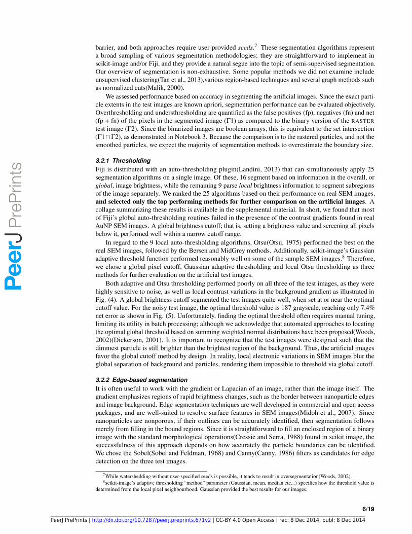
3.3 Preprocessing: Contrast Enhancement and DenoisingBecause of the likelihood of contrast variation in SEM images, we considered what effects contrastenhancement would have on a low-contrast AuNP image, and how they might effect the subsequentsegmentation step. We applied the following three scikit-image histogram correction methods on the dimsample image: global equalization, adaptive equalization and contrast stretching(Robert Fisher, SimonPerkins, Ashley Walker, 2003). Since this image has a very narrow brightness distribution, each techniqueresulted in broadening as seen in Fig. (8a). To test how the segmentation would be affected, we appliedglobal Otsu thresholding using the default parameters in Fiji to the original and corrected images.

Fig. (8b) illustrates that Otsu sufficiently segments both the original and stretched images; but poorlysegments the equalized image. It shows that image dimness did not correspond with poor segmentation.This is not true in general, as there are several examples of contrast correction improving segmentationaccuracy(Salihah and Mashor, 2010)(Humayun and Malik, 2013). Furthermore, workflows involvinghuman judgements, particularly in medical imaging, benefit from contrast correction in another facet: itmitigates bias arising from perceived image quality(Isa et al., 2003). Differences in images, segmentationstyles and contrast correction techniques make it difficult to conclude if contrast correction is generallyfavorable or unfavorable in AuNP workflows.

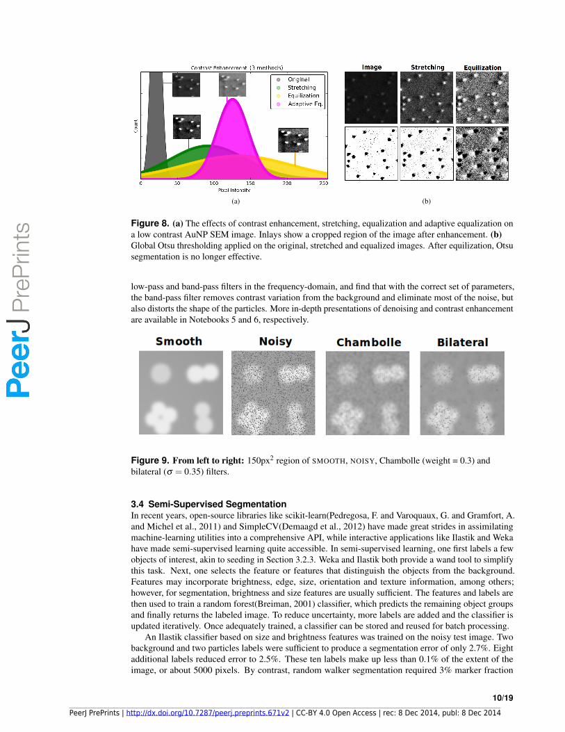
By far, the noisy test image was the most difficult to segment, and so was the subject of four denoisingapproaches, starting with mean and median rank filters(Soille, 2001). Mean filtering tends to degradeparticle boundaries by oversmoothing. The median filter sharpens boundaries and works well for sparsenoise, but performs poorly for the 25% corruption of the noisy image. Next, we applied a bilateralfilter(Tomasi, C., Manduchi, 1998) and the Chambolle(Chambolle, 2004) total variation filter. Thebilateral filter smooths while preserving boundaries, so it combines the strengths of both the mean andmedian filters. Both the bilateral and Chambolle methods outperformed standard rank filters and areshown in Fig. (8b). These four filters are all spatial-domain techniques. In Notebook 10, we demonstrate

9/19

PeerJ PrePrints | http://dx.doi.org/10.7287/peerj.preprints.671v2 | CC-BY 4.0 Open Access | rec: 8 Dec 2014, publ: 8 Dec 2014

PrePrin

ts

(a) (b)

Figure 8. (a) The effects of contrast enhancement, stretching, equalization and adaptive equalization ona low contrast AuNP SEM image. Inlays show a cropped region of the image after enhancement. (b)Global Otsu thresholding applied on the original, stretched and equalized images. After equilization, Otsusegmentation is no longer effective.

low-pass and band-pass filters in the frequency-domain, and find that with the correct set of parameters,the band-pass filter removes contrast variation from the background and eliminate most of the noise, butalso distorts the shape of the particles. More in-depth presentations of denoising and contrast enhancementare available in Notebooks 5 and 6, respectively.

Figure 9. From left to right: 150px2 region of SMOOTH, NOISY, Chambolle (weight = 0.3) andbilateral (σ = 0.35) filters.

3.4 Semi-Supervised SegmentationIn recent years, open-source libraries like scikit-learn(Pedregosa, F. and Varoquaux, G. and Gramfort, A.and Michel et al., 2011) and SimpleCV(Demaagd et al., 2012) have made great strides in assimilatingmachine-learning utilities into a comprehensive API, while interactive applications like Ilastik and Wekahave made semi-supervised learning quite accessible. In semi-supervised learning, one first labels a fewobjects of interest, akin to seeding in Section 3.2.3. Weka and Ilastik both provide a wand tool to simplifythis task. Next, one selects the feature or features that distinguish the objects from the background.Features may incorporate brightness, edge, size, orientation and texture information, among others;however, for segmentation, brightness and size features are usually sufficient. The features and labels arethen used to train a random forest(Breiman, 2001) classifier, which predicts the remaining object groupsand finally returns the labeled image. To reduce uncertainty, more labels are added and the classifier isupdated iteratively. Once adequately trained, a classifier can be stored and reused for batch processing.

An Ilastik classifier based on size and brightness features was trained on the noisy test image. Twobackground and two particles labels were sufficient to produce a segmentation error of only 2.7%. Eightadditional labels reduced error to 2.5%. These ten labels make up less than 0.1% of the extent of theimage, or about 5000 pixels. By contrast, random walker segmentation required 3% marker fraction

10/19

PeerJ PrePrints | http://dx.doi.org/10.7287/peerj.preprints.671v2 | CC-BY 4.0 Open Access | rec: 8 Dec 2014, publ: 8 Dec 2014

PrePrin

ts

(2×105 pixels) to reach the same accuracy, and the labels were spread out more uniformly across theimage. Size and brightness features worked well in segmenting our NOISY test image because, while thenoise can be as bright as the particles in some regions, it is still composed of singular pixels. Therefore,it can be distinguished based on size features. A classifier privy to brightness information alone couldnot segment NOISY. This is reflected in Fig. 2 where the noise contribution to the overall brightnesseffectively couples the background and particles distributions, which are otherwise separate and can besegmented trivially through a pixel threshold cutoff.

A salient restriction of classification approaches is the requisite of feature consistency betweenimages. This is illustrated in Fig. (10), in which a classifier trained on the noisy image is used tosegment the smoothed image, resulting in a doubling of overthresholding (false positives). This hasimportant implications for classification in batch processing, since even under careful SEM operation, itcan be difficult to obtain images with brightness and sharpness, especially for small particles on roughsurfaces. In such cases, preprocessing, in particular contrast equalization, can improve sample-to-sampleconsistency prior to segmentation. A workflow that incorporated contrast equalization would complementa classifier trained on evenly illuminated images. When switching between magnifications or detectors,we recommend separate classifier for each case.

(a) (b)

Figure 10. Segmentation error visualized: an Ilastik classifier was trained on, and subsequently used tosegment, the NOISY test image (a). The same classifier was then used to segment the SMOOTH test image(b). Since the classifier is trained to expect noise, it actually performs worse on a noise-free image likeSMOOTH. In general, the predictive power of a classifier will decline with the degree of dissimilaritybetween the training data and the sample data. The true particle extents are shown in grey, while red andgreen depict regions of overthresholding (fp) and underthresholding (fn), respectively.

3.5 Descriptors and MeasurementsOnce the particles have been segmented and labeled via connected-component algorithms(Wagner andLipinski, 2013), one typically generates distributions and statistics based on particle descriptors such asarea, perimeter and circularity

(C = 4π×Area/Perim2). Particle descriptors are returned from encoding

methods(K Benkrid, 2000) based on generalized morphological operations. This may result in errantdescriptors for small particles, especially those with curved edges. For circular particles, one may expectthe deviation to vary geometrically; that is, from a single pixel square (C=0.785) to a perfectly rasteredcircle (C=1.0), but this tends not to be the case(Hughes, 2014b). Fig. (11) shows the circularity as afunction of radius measured with the default encoding methods of scikit-image, Fiji/ImageJ and thea separate algorithm in the ImageJ Particles8 plugin.(Landini, 2008). Fiji’s default encoding actuallycorrects for small-pixel circularity and results in C=1 for circles of radii 50 pixels or greater. The Particles8plugin correctly estimates the single pixel square circularity. It is therefore very important be aware ofmeasurement errors arising from the encoding and digitization of the particles themselves.

11/19

PeerJ PrePrints | http://dx.doi.org/10.7287/peerj.preprints.671v2 | CC-BY 4.0 Open Access | rec: 8 Dec 2014, publ: 8 Dec 2014

PrePrin

ts

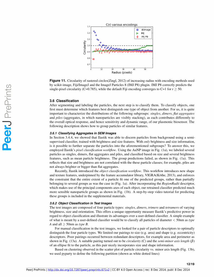
Figure 11. Circularity of rastered circles(Zingl, 2012) of increasing radius with encoding methods usedby scikit-image, Fiji/ImageJ and the ImageJ Particles 8 (IMJ P8) plugin. IMJ P8 correctly predicts thesingle-pixel circularity (C=0.785), while the default Fiji encoding converges to C=1 for r ≥ 50.

3.6 ClassificationAfter segmenting and labeling the particles, the next step is to classify them. To classify objects, onefirst must determine which features best distinguish one type of object from another. For us, it is quiteimportant to characterize the distributions of the following subgroups: singles, dimers, flat aggregatesand piles (aggregates, in which nanoparticles are visibly stacking), as each contributes differently tothe overall optical response, and hence sensitivity and dynamic range, of our plasmonic biosensor. Thefollowing description shows how to group particles of similar features.

3.6.1 Classifying Aggregates in SEM ImagesIn Section 3.4.4, we showed that Ilastik was able to discern particles from background using a semi-supervised classifier, trained with brightness and size features. With only brightness and size information,is it possible to further separate the particles into the aforementioned subgroups? To answer this, weemployed Ilastik’s pixel classification workflow. Using the AuNP image in Fig. (1a), we labeled severalparticles as singles, dimers, flat aggregates and piles, and classified based on size and several brightnessfeatures, such as mean particle brightness. The group predictions failed, as shown in Fig. (1a). Thisreflects that size and brightness are not correlated with the these particle classes; for example, piles arenot always brighter or bigger than flat aggregates.

Recently, Ilastik introduced the object classification workflow. This workflow introduces new shapeand texture features, underpinned by the feature accumulator library, VIGRA(Kothe, 2013), and enforcesthe constraint that the entire extent of a particle fit one of the predicted groups, rather than partiallybelonging to several groups as was the case in (Fig. 1a). After incorporating the RegionRadii descriptor,which makes use of the principal components axes of each object, our retrained classifier predicted muchmore sensible nanoparticle groups as shown in Fig. (1b). A step-by-step video tutorial for predictingthese groups is included in the supplemental materials.

3.6.2 Object Classification in Test ImagesThe test images are composed of four particle types: singles, dimers, trimers and tetramers of varyingbrightness, size and orientation. This offers a unique opportunity measure Ilastik’s predictive power inregard to object classification and illustrate its advantages over a user-defined classifier. A simple exampleof what is meant by a user-defined classifier would be to classify all particles of diameter < 50nm as typeA and all ≥ 50nm as type B.

For manual classification in the test images, we looked for a pair of particle descriptors to optimallydistinguish the four particle types. We limited our pairings to size (e.g. area) and shape (e.g. eccentricity)descriptors. Poor pairings occurred between redundant descriptors, for example area and perimeter asshown in Fig. (13a). A suitable pairing turned out to be circularity (C) and the semi-minor axis length (β )of an ellipse fit to the particle, as this pair nicely incorporates size and shape information.

Based on clustering observed in the scatter plot of particle circularity vs. minor axis length (Fig. 13b),we used pyparty to define the following partition (shown as white dotted lines):

12/19

PeerJ PrePrints | http://dx.doi.org/10.7287/peerj.preprints.671v2 | CC-BY 4.0 Open Access | rec: 8 Dec 2014, publ: 8 Dec 2014

PrePrin

ts

(a) (b)

(c) (d)

Figure 12. Ilastik predictions of singles, dimers, flat aggregates and piles on a zoomed region ofimage from Fig. (1a). Predictions from pixel classification workflow (b) and object classificationworkflow (c). Pie chart (d) indicates the number of particles identified in the full image. Wedge size isproportional to the area covered by each group. The net particle area is 24.93% of the total image area.

Singles = (β < 42, C > 0.85) Dimers = (β < 42, C < 0.85)Trimers = (β > 42, C > 0.6) Tetramers = (β > 42, C < 0.6) (1)

Ten particles were labeled to train the Ilastik classifier: 3 tetramers, 3 trimers, 2 singles and 2dimers, using the descriptors Count9 and RegionRadii, rather than circularity and minor axis length. Thedescriptors are different because the manual partitioning was done in pyparty, which utilizes descriptorsdefined in scikit-image, rather than VIGRA. Two challenges with manual partitioning are apparent: first,for more than two feature dimensions, one must define an n-dimensional feature space, and the cutsbecome hyperplanes which are impractical to implement. Secondly, finding the optimal cuts is non-trivial.Ilastik nicely automates both of these tasks.

Ilastik’s predictions and the true groups are shown in Fig. (14). The manually assigned partitionsare filled in with bold color. It is clear that the fixed partition poorly separates the trimers and tetramers,as it misidentified 53 trimers and tetramers or about 18% of the total trimer/tetramer population. By

9In VIGRA, the Count descriptor is merely is the number of pixels in the object, so it is equivalent to the Area descriptor inscikit-image.

13/19

PeerJ PrePrints | http://dx.doi.org/10.7287/peerj.preprints.671v2 | CC-BY 4.0 Open Access | rec: 8 Dec 2014, publ: 8 Dec 2014

PrePrin

ts

(a) (b)

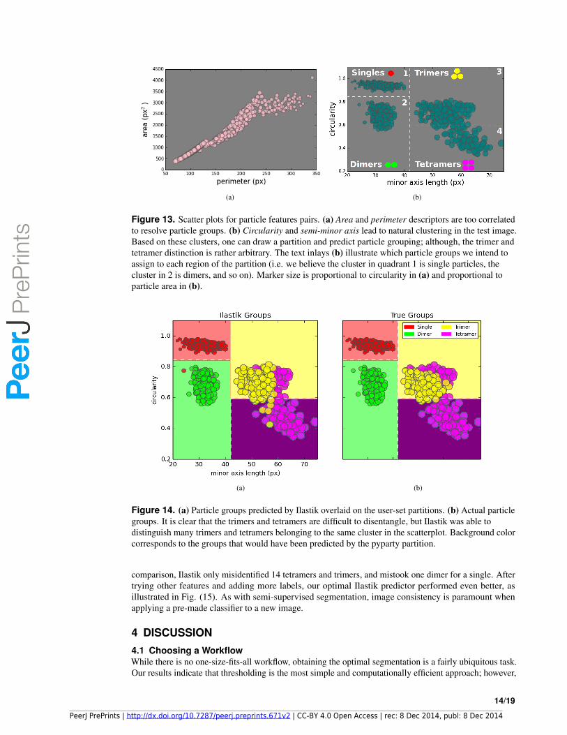
Figure 13. Scatter plots for particle features pairs. (a) Area and perimeter descriptors are too correlatedto resolve particle groups. (b) Circularity and semi-minor axis lead to natural clustering in the test image.Based on these clusters, one can draw a partition and predict particle grouping; although, the trimer andtetramer distinction is rather arbitrary. The text inlays (b) illustrate which particle groups we intend toassign to each region of the partition (i.e. we believe the cluster in quadrant 1 is single particles, thecluster in 2 is dimers, and so on). Marker size is proportional to circularity in (a) and proportional toparticle area in (b).

(a) (b)

Figure 14. (a) Particle groups predicted by Ilastik overlaid on the user-set partitions. (b) Actual particlegroups. It is clear that the trimers and tetramers are difficult to disentangle, but Ilastik was able todistinguish many trimers and tetramers belonging to the same cluster in the scatterplot. Background colorcorresponds to the groups that would have been predicted by the pyparty partition.

comparison, Ilastik only misidentified 14 tetramers and trimers, and mistook one dimer for a single. Aftertrying other features and adding more labels, our optimal Ilastik predictor performed even better, asillustrated in Fig. (15). As with semi-supervised segmentation, image consistency is paramount whenapplying a pre-made classifier to a new image.

4 DISCUSSION4.1 Choosing a WorkflowWhile there is no one-size-fits-all workflow, obtaining the optimal segmentation is a fairly ubiquitous task.Our results indicate that thresholding is the most simple and computationally efficient approach; however,

14/19

PeerJ PrePrints | http://dx.doi.org/10.7287/peerj.preprints.671v2 | CC-BY 4.0 Open Access | rec: 8 Dec 2014, publ: 8 Dec 2014

PrePrin

ts

Figure 15. Incorrect predictions for particle groups in the test images. The trimers and tetramers weremisidentified more often than the singles and dimers. Ilastik clearly outperforms the fixed partitionapproach (Fig. 13b), which mislabeled 53 of the trimers as tetramers. Predictions based on 10 labeledparticles in Ilastik using Count and RegionRadii features mislabeled only 14 trimer/tetramers and 1single/double. An optimal predictor based on 20 labeled particles and the additional feature of Mean inneighborhood mislabeled only six trimers.

it demands that particles are necessarily brighter than the background and the image is fairly noise-free.Whenever objects and background have intersecting brightness distributions, they can no longer bedelineated through brightness features alone. In the test images, noise and smoothing resulted in thisconvolution (see the overlapping regions in Fig. 2 histogram); therefore, it is not surprising that seedingand semi-supervised methods performed much better on these images. In many cases, preprocessingcan improve the workflow; however, care should be taken to understand any compounding effects orconstraints it may impose on the subsequent segmentation step. In regard to classifying different groupsof nanoparticle species, Ilastik’s object classification workflow is quite powerful; we recommend it highly.In cases of poor image consistently, it may still be advantageous to classify particles based on a hard-setpartition (e.g. radius ≥ 50px & circularity < 0.8), and straightforward API for such tasks.

Because of the subjective nature of image processing(Woods, 2002), discovering an optimal, robustworkflow usually requires trial and error. It is important to choose tools commensurate with researchgoals and programming experience. Graphical interfaces like those found in Fiji and Ilastik offer auser-friendly avenue to rapidly explore a variety of techniques. Working directly with the scikit-imageAPI provides a nice trade-off between productivity and flexibility, and is great for building customizedworkflows. Ultimately, as customizability becomes more important, the tradeoff between flexibility andproductivity leads away from graphical applications like Fiji and Ilastik, towards flexible API’s like thosefound in scikit-image. In high-performance applications, OpenCV(Bradski, 2000) or GPU-acceleratedlibraries(NVIDIA, 2014) may offer the best framework. In any case, optimizing the image processingworkflow is time consuming, so obtaining a good image is better than relying on processing to compensate.

4.2 Imaging Beyond SEMIn addition to SEM, one may also consider using TEM or STEM (scanning transmission electron mi-croscopy) to enhance contrast and reduce charging; however, transmission microscopy requires transparentsamples, or in the case of STEM, distributing the nanoparticles onto a carbon support film(Pennycooket al., 2007). Scanning probe techniques like atomic force microscopy (AFM) offer a viable alternativeto electron microscopy. Nanopositioning stages facilitate wide-field AFM imaging, while maintainingresolutions comparable to, or better than, those of typical SEM images at the same magnification(Andradeet al., 2013). AFM yields new operational constraints, such as considerations in regard to tip size and

15/19

PeerJ PrePrints | http://dx.doi.org/10.7287/peerj.preprints.671v2 | CC-BY 4.0 Open Access | rec: 8 Dec 2014, publ: 8 Dec 2014

PrePrin

ts

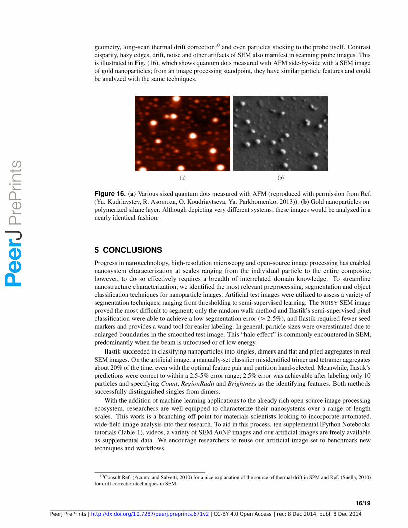
geometry, long-scan thermal drift correction10 and even particles sticking to the probe itself. Contrastdisparity, hazy edges, drift, noise and other artifacts of SEM also manifest in scanning probe images. Thisis illustrated in Fig. (16), which shows quantum dots measured with AFM side-by-side with a SEM imageof gold nanoparticles; from an image processing standpoint, they have similar particle features and couldbe analyzed with the same techniques.

(a) (b)

Figure 16. (a) Various sized quantum dots measured with AFM (reproduced with permission from Ref.(Yu. Kudriavstev, R. Asomoza, O. Koudriavtseva, Ya. Parkhomenko, 2013)). (b) Gold nanoparticles onpolymerized silane layer. Although depicting very different systems, these images would be analyzed in anearly identical fashion.

5 CONCLUSIONSProgress in nanotechnology, high-resolution microscopy and open-source image processing has enablednanosystem characterization at scales ranging from the individual particle to the entire composite;however, to do so effectively requires a breadth of interrelated domain knowledge. To streamlinenanostructure characterization, we identified the most relevant preprocessing, segmentation and objectclassification techniques for nanoparticle images. Artificial test images were utilized to assess a variety ofsegmentation techniques, ranging from thresholding to semi-supervised learning. The NOISY SEM imageproved the most difficult to segment; only the random walk method and Ilastik’s semi-supervised pixelclassification were able to achieve a low segmentation error (≈ 2.5%), and Ilastik required fewer seedmarkers and provides a wand tool for easier labeling. In general, particle sizes were overestimated due toenlarged boundaries in the smoothed test image. This “halo effect” is commonly encountered in SEM,predominantly when the beam is unfocused or of low energy.

Ilastik succeeded in classifying nanoparticles into singles, dimers and flat and piled aggregates in realSEM images. On the artificial image, a manually-set classifier misidentified trimer and tetramer aggregatesabout 20% of the time, even with the optimal feature pair and partition hand-selected. Meanwhile, Ilastik’spredictions were correct to within a 2.5-5% error range; 2.5% error was achievable after labeling only 10particles and specifying Count, RegionRadii and Brightness as the identifying features. Both methodssuccessfully distinguished singles from dimers.

With the addition of machine-learning applications to the already rich open-source image processingecosystem, researchers are well-equipped to characterize their nanosystems over a range of lengthscales. This work is a branching-off point for materials scientists looking to incorporate automated,wide-field image analysis into their research. To aid in this process, ten supplemental IPython Notebookstutorials (Table 1), videos, a variety of SEM AuNP images and our artificial images are freely availableas supplemental data. We encourage researchers to reuse our artificial image set to benchmark newtechniques and workflows.

10Consult Ref. (Acunto and Salvetti, 2010) for a nice explanation of the source of thermal drift in SPM and Ref. (Snella, 2010)for drift correction techniques in SEM.

16/19

PeerJ PrePrints | http://dx.doi.org/10.7287/peerj.preprints.671v2 | CC-BY 4.0 Open Access | rec: 8 Dec 2014, publ: 8 Dec 2014

PrePrin

ts

6 SUPPLEMENTALSupplemental Notebooks (Table 1), figures and videos are hosted at: https://github.com/hugadams/imgproc_supplemental. The Notebooks are presented in tutorial format to provide alaunching point into particle analysis.

7 ACKNOWLEDGEMENTSThis research is supported by the George Gamow Research and Luther Rice Collaborative Researchfellowship programs, as well as the George Washington University (GWU) Knox fellowship. We thankthe GWU School of Engineering and Applied Science for the training and extended use of the SEM. Weare indebted to Annie Matsko for batch measurements of particle size and segmentation, and in assistanceof sample preparation, proofreading, and imaging. We also acknowledge Clay Morton and Julie Veenstrafor their measurements in Ilastik.

17/19

PeerJ PrePrints | http://dx.doi.org/10.7287/peerj.preprints.671v2 | CC-BY 4.0 Open Access | rec: 8 Dec 2014, publ: 8 Dec 2014

PrePrin

ts

REFERENCES

Acunto, M. D. and Salvetti, O. (2010). Image analysis aided by Segmentation algorithms for techniques ranging from ScanningProbe Microscopy to Optical Microscopy. Microscopy: Science; Technology; Applications and Education, pages 1455–1466.

Alexander, S. K., Azencott, R., Bodmann, B. G., Bouamrani, A., Chiappini, C., Ferrari, M., Liu, X., and Tasciotti, E. (2009). SEMImage Analysis for Quality Control of Nanoparticles. Proceedings of the 13th International Conference on Computer Analysis ofImages and Patterns, pages 590–597.

Amako, J., Nagasaka, K., and Kazuhiro, N. (2002). Chromatic-distortion compensation in splitting and focusing of femtosecondpulses by use of a pair of diffractive optical elements. Optics letters, 27(11):969–71.

Amendola, V. and Meneghetti, M. (2009). Size Evaluation of Gold Nanoparticles by UV - vis Spectroscopy. Journal of PhysicalChemistry C, 113:4277–4285.

Andrade, J. E. D., Machado, R., Macedo, M. A., Guilherme, F., and Cunha, C. (2013). AFM and XRD Characterization of SilverNanoparticles Films Deposited on the Surface of DGEBA Epoxy Resin by Ion Sputtering. SciELO, 23:19–23.

Arganda-Carreras, I., Cardona, A., Kaynig, V., Schindelin, J. (2011). Trainable Weka Segmentation. http://fiji.sc/Trainable_Weka_Segmentation.

Barlow, S. (2004). CLASSES IN ELECTRON MICROSCOPY AT SDSU: Electron Microscope Facility, San Diego State University.http://www.sci.sdsu.edu/emfacility/555class/class1.html.

Becker, J., Trugler, A., Jakab, A., Hohenester, U., and Sonnichsen, C. (2010). The Optimal Aspect Ratio of Gold Nanorods forPlasmonic Bio-sensing. Plasmonics, 5(2):161–167.

Beucher, S ; Lantuejoul, C. (1979). Use of watersheds in contour detection. In Proceedings of the International Workshop of ImageProcessing, Real-time Edge and Motion Detection.

Bradski, G. (2000). OpenCV. Dr. Dobb’s Journal of Software Tools.Breiman, L. (2001). Random Forests. Machine Learning, 45:5–32.Canny, J. (1986). A Computational Approach to Edge Detection. IEEE Trans. Pattern Analysis and Machine Intelligence, 8:679–714.Chambolle, A. (2004). An algorithm for total variation minimization and applications. Journal of Mathematical Imaging and Vision,

20:89–97.Cheng, Y., Wang, M., Borghs, G., and Chen, H. (2011). Gold Nanoparticle Dimers for Plasmon Sensing. Langmuir, 27:7884–7891.Coelho, L. P. (2013). Mahotas : Open source software for scriptable computer vision. Journal of Open Research Software, 1:1–7.Cressie, N. and Serra, J. (1988). Image analysis and mathematical morphology: 2nd Edition. Academic Press, London; New York,

2 edition.Dellby, N., Krivanek, O. L., Nellist, P. D., Batson, P. E., and Lupini, a. R. (2001). Progress in aberration-corrected scanning

transmission electron microscopy. Microscopy, 50(3):177–185.Demaagd, K., Oliver, A., Oostendorp, N., and Scott, K. (2012). Practical Computer Vision with SimpleCV: The Simple Way to Make

Technology See. O’Reily Media, Inc.Dickerson, J. A. (2001). ISU EE528: Chapter 5 Segmentation. http://www.eng.iastate.edu/ee528/

sonkamaterial/chapter_5.htm.Ding, L. and Goshtasby, A. (2001). On the Canny edge detector. Pattern Recognition, 34(January 2000):721–725.Editorial (2014). Software with impact. Nature Methods, 11(3):211–211.Eliceiri, K. W., Berthold, M. R., Goldberg, I. G., Ibanez, L., Manjunath, B. S., Martone, M. E., Murphy, R. F., Peng, H., Plant, A. L.,

Roysam, B., Stuurman, N., Stuurmann, N., Swedlow, J. R., Tomancak, P., and Carpenter, A. E. (2012). Biological imagingsoftware tools. Nature methods, 9(7):697–710.

Gleber, G., Cibik, L., Haas, S., Hoell, A., Muller, P., and Krumrey, M. (2010). Traceable size determination of PMMA nanoparticlesbased on Small Angle X-ray Scattering (SAXS). Journal of Physics: Conference Series, 247:012027.

Grady, L. (2006). Random walks for image segmentation. IEEE transactions on pattern analysis and machine intelligence,28(11):1768–83.

Green, B. (2002). Canny Edge Detection Tutorial. http://dasl.mem.drexel.edu/alumni/bGreen/www.pages.drexel.edu/_weg22/can_tut.html.

Haiss, W., Thanh, N. T. K., Aveyard, J., and Fernig, D. G. (2007). Determination of size and concentration of gold nanoparticlesfrom UV-vis spectra. Analytical Chemistry, 79(11):4215–21.

Hughes, A. (2014a). AuNP Image Processing Supplemental Data. https://github.com/hugadams/imgproc_supplemental.

Hughes, A. (2014b). ImageJ Mailing list archive: “Circularity Error?”. http://comments.gmane.org/gmane.comp.java.imagej/31695.

Hughes, A. (2014c). pyparty: Blob Detection, Drawing and Manipulation in Python. Journal of Open Research Software, 2:2–6.Humayun, J. and Malik, A. S. (2013). Fusion of Local Rank Transform and Tone Mapping for Contrast Enhancement: Application

to Skin Lesion Image Analysis. IFMBE Proceedings, 39:935–938.Isa, M., Ashidi, N., Mashor, M., and Othman, N. (2003). Contrast Enhancement Image Processing Technique on Segmented Pap

Smear Cytology Images.Jans, H., Liu, X., Austin, L., Maes, G., and Huo, Q. (2009). Dynamic light scattering as a powerful tool for gold nanoparticle

bioconjugation and biomolecular binding studies. Analytical chemistry, 81(22):9425–32.JEOL (2014). A Guide to Scanning Microscope Observation. Technical report.Jeong, H.-H., Erdene, N., Lee, S.-K., Jeong, D.-H., and Park, J.-H. (2011). Fabrication of fiber-optic localized surface plasmon

resonance sensor and its application to detect antibody-antigen reaction of interferon-gamma. Optical Engineering, 50(12).K Benkrid, D. C. (2000). Design and FPGA Implementation of a Perimeter Estimator. Technical report, The Queen’s University of

Belfast.Kessentini, S. and Barchiesi, D. (2012). Quantitative comparison of optimized nanorods, nanoshells and hollow nanospheres for

photothermal therapy. Biomedical optics express, 3(3):590–604.Khlebtsov, B. N. and Khlebtsov, N. G. (2011). On the measurement of gold nanoparticle sizes by the dynamic light scattering

method. Colloid Journal, 73(1):118–127.Khlebtsov, N. (2008). Determination of Size and Concentration of Gold Nanoparticles from Extinction Spectra. Analytical

18/19

PeerJ PrePrints | http://dx.doi.org/10.7287/peerj.preprints.671v2 | CC-BY 4.0 Open Access | rec: 8 Dec 2014, publ: 8 Dec 2014

PrePrin

ts

Chemistry, 80(17):6620–6625.Kim, T., Lee, C., Joo, S., and Lee, K. (2008). Kinetics of Gold Nanoparticle Aggregation: Experiments and Modeling. Journal of

Colloid Interface Science, 2(318):238–243.Klein, T., Buhr, E., Johnsen, K.-P., and Frase, C. G. (2011). Traceable measurement of nanoparticle size using a scanning electron

microscope in transmission mode (TSEM). Measurement Science and Technology, (22).Kothe, U. (2013). The VIGRA Image Analysis Library, Version 1.10.Kovesi, P. D. (2000). MATLAB and Octave functions for computer vision and image processing. http://www.csse.uwa.

edu.au/$\sim$pk/Research/MatlabFns/.Landini, G. (2008). Advanced shape analysis with ImageJ. In Second ImageJ user and developer Conference, Lexembourg.Landini, G. (2013). Auto Threshold and Auto Local Threshold.Lehmann, T. (1999). Survey: Interpolation methods in medical image processing. Medical Imaging, IEEE . . . , 18(11):1049–1075.Lopatynskyi, A. M., Lopatynska, O. G., Guo, L. J., and Chegel, V. I. (2011). Localized Surface Plasmon Resonance Biosensor—Part

I: Theoretical Study of Sensitivity—Extended Mie Approach, volume 11.Malik, J. (2000). Normalized cuts and image segmentation. IEEE Transactions on Pattern Analysis and Machine Intelligence,

22(8):888–905.Mascarelli, A. (2014). Research tools: Jump off the page. Nature Jobs, 507:523–525.MathWorks (2013). MATLAB: The Language of Technical Computing.McKenna, P. (2012). Nanoparticles Make Steam without Bringing Water to a Boil. MIT Technology Review.Meli, F., Klein, T., Buhr, E., Frase, C. G., Gleber, G., Krumrey, M., Duta, A., Duta, S., Korpelainen, V., Bellotti, R., Picotto, G. B.,

Boyd, R. D., and Cuenat, A. (2012). Traceable size determination of nanoparticles, a comparison among European metrologyinstitutes. Measurement Science and Technology, 23(12):125005.

Microscopy, C. Z. (2014). ZEISS EVO Your High Definition SEM with Workflow Automation Increased Resolutionand Surface Detail for All Samples: Version 1.3. http://applications.zeiss.com/C125792900358A3F/0/A7A32858228B4D46C1257BBB004E6E74/$FILE/EN_42_011_092_EVO.pdf.

Midoh, Y., Nakamae, K., and Fujioka, H. (2007). Object size measurement method from noisy SEM images by utilizing scale space.Measurement Science and Technology, 18(3):579–591.

Moirangthem, R. S., Chang, Y.-C., and Wei, P.-K. (2011). Ellipsometry study on gold-nanoparticle-coated gold thin film forbiosensing application. Biomedical optics express, 2(9):2569–76.

Narkhede, H. P. (2013). Review of Image Segmentation Techniques. International Journal of Science and Modern Engineering,(8):54–61.

Nath, N. and Chilkoti, A. (2002). A colorimetric gold nanoparticle sensor to interrogate biomolecular interactions in real time on asurface. Analytical chemistry, 74(3):504–9.

Nemota, F. T. M. D. S. (2012). A Statistical Model of Signal-Noise in Scanning Electron Microscopy. Scanning, 34(137).NVIDIA (2014). NVIDIA CUDA ZONE: NVIDIA Performance Primitives. https://developer.nvidia.com/npp.Otsu, N. (1975). A threshold selection method from gray-level histograms. Automatica, C(1):62–66.Pease, L. F., Tsai, D.-H., Hertz, J. L., Zangmeister, R. a., Zachariah, M. R., and Tarlov, M. J. (2010). Packing and size determination

of colloidal nanoclusters. Langmuir : the ACS journal of surfaces and colloids, 26(13):11384–90.Pedregosa, F. and Varoquaux, G. and Gramfort, A. and Michel, V., and Thirion, B. and Grisel, O. and Blondel, M. and Prettenhofer,

P., , and Weiss, R. and Dubourg, V. and Vanderplas, J. and Passos, A., and Cournapeau, D. and Brucher, M. and Perrot, M. andDuchesnay, E. (2011). Scikit-learn: Machine Learning in Python. Journal of Machine Learning Research, 12:2825–2830.

Pennycook, S. J., Lupini, A. R., Varela, M., Borisevich, A. Y., Peng, Y., Oxley, M. P., van Benthem, K., and Chisholm, M. F. (2007).Scanning Transmission Electron Microscopy for Nanostructure Characterization.

Perez, F. and Granger, B. (2007). IPython: a Stystem for Interactive Scientific Computing. Computing in Science and Engineering,9(3):21–29.

Peterson, E. J. T. O. P. (2001). Scipy: Open source scientific tools for Python.Ploshnik, E., Langner, K. M., Halevi, A., Ben-Lulu, M., Muller, A. H. E., Fraaije, J. G. E. M., Agur Sevink, G. J., and Shenhar, R.

(2013). Hierarchical Structuring in Block Copolymer Nanocomposites through Two Phase-Separation Processes Operating onDifferent Time Scales. Advanced Functional Materials, 23(34):4215–4226.

Reetz, M. T., Maase, M., Schilling, T., and Tesche, B. (2000). Computer Image Processing of Transmission Electron MicrographPictures as a Fast and Reliable Tool To Analyze the Size of Nanoparticles. The Journal of Physical Chemistry B, 104(37):8779–8781.

Robert Fisher, Simon Perkins, Ashley Walker, E. W. (2003). Image Processing Learning Resources: Contrast Stretching.Sai, V. V. R., Kundu, T., and Mukherji, S. (2009). Novel U-bent fiber optic probe for localized surface plasmon resonance based

biosensor. Biosensors bioelectronics, 24(9):2804–9.Salihah, A. A. and Mashor, M. (2010). Improving colour image segmentation on acute myelogenous leukaemia images using

contrast enhancement techniques. . . . IECBES), 2010 IEEE . . . , (December):246–251.Sankur, M. S. and Lent, B. (2004). Survey over image thresholding techniques and quantitative performance evaluation. Journal of

Electronic Imaging, 13(1):146–168.Sbalzarini, I. and Kournoutsakos, P. (2005). Feature Point Tracking and Trajectory Analysis for Video Imaging in Cell Biology.

Journal of Structural Biology, 2(151):182–195.Schindelin, J., Arganda-Carreras, I., Frise, E., Kaynig, V., Longair, M., Pietzsch, T., Preibisch, S., Rueden, C., Saalfeld, S., Schmid,

B., Yinevez, J.-Y., James White, D., Hartenstein, V., Eliceiri, K., Pavel, T., and Cardona, A. (2012). Fiji: an open-source platformfor biological-image analysis. Nature Methods, 9(7):676–682.

Schneider, C.A., Rasband, W.S., Eliceiri, K. (2012). NIH Image to ImageJ: 25 years of image analysis. Nature Methods: Focus onBioimage Informatics, 9(7):671–675.

Sciacca, B. and Monro, T. M. (2014). Dip biosensor based on localized surface plasmon resonance at the tip of an optical fiber.Langmuir : the ACS journal of surfaces and colloids, 30(3):946–54.

Shahin, S., Gangopadhyay, P., and Norwood, R. a. (2012). Ultrathin organic bulk heterojunction solar cells: Plasmon enhancedperformance using Au nanoparticles. Applied Physics Letters, 101(5):053109.

Singh, S. (2013). Microscopic Image Analysis of Nanoparticles by Edge Detection Using Ant Colony Optimization. IOSR Journal

19/19

PeerJ PrePrints | http://dx.doi.org/10.7287/peerj.preprints.671v2 | CC-BY 4.0 Open Access | rec: 8 Dec 2014, publ: 8 Dec 2014

PrePrin

ts

of Computer Engineering, 11(3):84–89.Snella, M. (2010). Drift Correction for Scanning-Electron Microscopy. Masters thesis, Massachusetts Institute of Technology.Sobel, I. and Feldman, G. (1968). A 3x3 Isotropic Gradient Operator for Image Processing a talk at the Stanford Artificial Project in

1968. In Stanford Artificial Intelligence Project, Stanford.Soille, P. (2001). On morphological operators based on rank filters. Pattern Recognition, 35:527–535.Sommer, C., Straehle, C., Kothe, U., and Hamprecht, F. (2011). ilastik: Interactive Learning and Segmentation Toolkit. In 8th IEEE

International Symposium on Biomedial Imaging (ISBI).Sumengen, B. and Manjunath, B. S. (2005). MULTI-SCALE EDGE DETECTION AND IMAGE SEGMENTATION. In Proc.

European Signal Processing Conference (EUSIPCO).Tan, K. S., Mat Isa, N. A., and Lim, W. H. (2013). Color image segmentation using adaptive unsupervised clustering approach.

Applied Soft Computing, 13(4):2017–2036.Tomasi, C., Manduchi, R. (1998). Bilateral Filtering for Gray and Color Images. In Proceedings of the1998 IEEE International

Conference on Computer Vision, Bombay, India.Turkevich, J., Stevenson, P. C., and Hillier, J. (1951). A study of the nucleation and growth processes in the synthesis of colloidal

gold. Discussions of the Faraday Society, 11:55.van der Walt, S., Nunez-Iglesias, J., Boulogne, F., Warner, J., and Al, E. (2014). scikit-image: image processing in Python. PeerJ,

(453).Wagner, T. and Lipinski, H. (2013). IJBlob : An ImageJ Library for Connected Component Analysis and Shape Analysis. Journal

of Open Research Software, 1(6):6–8.Woods, R. C. G. R. E. (2002). Digital Image Processing. Prentice Hall, Upper Saddle River, New Jersey, 2nd edition.Yu. Kudriavstev, R. Asomoza, O. Koudriavtseva, Ya. Parkhomenko, K. M. (2013). AFM/EFM Study of InSb Quantum Dots Grown

by LPE on InAs Substrates. In XXII INTERNATIONAL MATERIALS RESEARCH CONGRESS, Cancun, Mexico.Zingl, A. (2012). A Rasterizing Algorithm for Drawing Curves. Multimedia und Softwareentwicklung.

20/19

PeerJ PrePrints | http://dx.doi.org/10.7287/peerj.preprints.671v2 | CC-BY 4.0 Open Access | rec: 8 Dec 2014, publ: 8 Dec 2014

PrePrin

ts