a weighted goal programming approach to fuzzy...

TWMS J. App. Eng. Math. V.6, N.2, 2016, pp.193-212

A WEIGHTED GOAL PROGRAMMING APPROACH TO FUZZY

LINEAR REGRESSION WITH QUASI TYPE-2 FUZZY

INPUT-OUTPUT DATA

E.HOSSEINZADEH1, H.HASSANPOUR1, M.AREFI2, M.AMAN1, §

Abstract. This study attempts to develop a regression model when both input dataand output data are quasi type-2 fuzzy numbers. To estimate the crisp parameters ofthe regression model, a linear programming model is proposed based on goal program-ming. To handle the outlier problem, an omission approach is proposed. This approachexamines the behavior of value changes in the objective function of proposed modelwhen observations are omitted. In order to illustrate the proposed model, some numer-ical examples are presented. The applicability of the proposed method is tested on areal data set on soil science. The predictive performance of the model is examined bycross-validation.

Keywords: fuzzy linear regression, goal programming, type-2 fuzzy set, uncertainty, quasitype-2 fuzzy number.

AMS Subject Classification: 03E72, 90C05, 62J86, 62J05.

1. Introduction

Type-2 fuzzy logic is increasingly being advocated as a methodology for reasoning insituations where high uncertainties are present. Type-2 fuzzy sets were first presented byZadeh in 1975 [42]. Mizumoto and Tanaka [27] further explored the logical operationsof type-2 fuzzy sets. In the later 1990s and into the new millennium the definitions oflogical operations for generalized type-2 fuzzy sets were completed [18, 24] and the firsttype-2 fuzzy logic textbook [23] published. Currently, the number of reported applicationsof interval type-2 fuzzy logic is growing year on year. The concept of type-2 fuzzy sets(T2FSs) was introduced by Zadeh [42] as an extension of the concept of ordinary fuzzysets (henceforth called type-1 fuzzy sets). T2FSs are characterized by fuzzy membershipfunctions (MF), i.e., the membership grades themselves are fuzzy sets in [0, 1]. Theyare very useful in circumstances where it is difficult to determine an exact membershipfunction for a fuzzy set; hence, they are useful for incorporating linguistic uncertainties,e.g., the words that are used in linguistic knowledge which can mean different things todifferent people [22]. As a way of illustration, suppose a number of people are asked

1 Faculty of Mathematical Science and Statistics, Department of Mathematics, University of Birjand,Birjand, I.R of Iran.e-mail: [email protected], [email protected], [email protected];

2 Faculty of Mathematical Science and Statistics, Department of Statistics, University of Birjand,Birjand, I.R of Iran.e-mail: [email protected];§ Manuscript received: March 03, 2015; accepted: July 30, 2015.

TWMS Journal of Applied and Engineering Mathematics Vol.6 No.2 c© Isık University, Departmentof Mathematics 2016; all rights reserved.

193

194 TWMS J. APP. ENG. MATH. V.6, N.2, 2016

about the temperature of the room where they are present. All the subjects mention“ approximately 70◦ Fahrenheit ”. Nonetheless, if each individual subject is asked toshow the “ approximately 70◦ Fahrenheit MF ”, different MFs are likely to be presented,even if the MFs are all of the same kind (e.g., triangular). This implies the statementthat “ Words can mean different things to different people ”[24]. Accordingly, T2FSsprove helpful in cases where an exact form of an MF cannot be determined. Karnik andMendel [18] introduced the centroid and generalized centroid of a type-II fuzzy set andexplained how to calculate them. Furthermore, they showed how to compute the centroidof interval and Gaussian type-II fuzzy sets. Karnik and Mendel [25] discussed set theoreticoperations for type-II sets, properties of membership grades of type-II fuzzy sets, and type-II relations and other compositions, and cartesian products under minimum and productt-norms. Mendel and John [25] defined a new representation theorem of type-II fuzzysets and introduced formulas for the union, intersection, and complement for type-II fuzzysets without applying Extension Principle, by using this new representation. Mendel [22]examined questions such as ”What is a type-II fuzzy set?”, ”the importance of definitionof type-II fuzzy sets”, ”How and why are type-II fuzzy sets used in rule-based systems?”.Mendel [22] described the important advances that have been made during the past fiveyears both general and interval type-II fuzzy sets and systems. Recently, Liu and Mendel[26] have presented the concept of quasi type-2 fuzzy system. This kind of system is astep forward to a more general kind of type-2 fuzzy system. The idea is developed on thebasis of the alpha-level representation for general type-2 fuzzy sets. Quasi type-2 fuzzysystems become interesting since they should be more robust to uncertainty than theirinterval type-2 counterparts.Regression analysis is one of the most widely used statistical techniques for determining therelationship between variables in order to describe or predict some stochastic phenomena.Research on fuzzy regression analysis began by Celmins [2], Diamond [5], and Tanaka etal. [37], and was continued by some authors, e.g., Kacprzyk and Fedrizzi [19]; Wang andTsaur [38]; Kao and Chyu [17]; D’Urso [6]; Wang et al. [39]; Nasrabadi et al. [30]; Hojatiet al. [14]; Modarres et al. [28]; Guo and Tanaka [7]; Coppi et al. [3]; Yao and Yu [41];Hassanpour et al. [10, 12, 11, 13]; Ramli et al. [35]; Kelkinnama and Taheri [20]; Kocadagli[21]. But, based on our best knowledge, there has not been any research on regressionanalysis for quasi type-2 fuzzy data. Recently, Rabiei et al. [34] have proposed a Least-squares approach to regression modeling for interval-valued fuzzy data. Also, Poleshchukand Komarov [33] have presented a regression model for interval type-2 fuzzy sets basedon the least squares estimation technique.The authors [15] have proposed a goal programming approach to calculate the regressioncoefficients of fuzzy linear regression model, when the inputs are crisp, but the outputsand regression coefficients are QT2FNs. In this paper, a similar method is applied tocalculate the coefficients of model when the independent variables (inputs), as well as theresponse variable (output), are QT2FNs and regression coefficient are assumed to be crispnumbers. To accomplish this, we introduce a distance on the space of quasi type-2 fuzzynumbers and a goal programming method to obtain the coefficients of regression model.Existing outliers in the data set, causes the result of fuzzy linear regression be incorrect.Chen [4], to reduce the effect of outliers, considered the minimization model of Tanaka[36] with n additional constraints. It is important for a data analyst to be able to identifyoutliers and assess their effect on various aspects of the analysis. Some methods have beenpresented to detect outliers in FLR [4, 32]. However, they have some drawbacks, e.g, theymust pre-assign some values to the parameters without any instructive suggestion to chosethem, and they cannot conduct a formal test for the outliers. To overcome the mentioned

E.HOSSEINZADEH, H.HASSANPOUR, M.AREFI, M.AMAN: A WEIGHTED GOAL... 195

shortcomings, we use an omission approach based on Hung and Yang method [16], whichexamines the value change in the objective function when some of the observations areomitted from the data set in QT2FLR model. Moreover, to define the cutoffs for outliers,we use the box plot procedure as a visual display tool.The remainder of the paper is organized as follows: Section 2, contains some preliminariesof quasi type-2 fuzzy set theory. Also, a distance between quasi type-2 fuzzy numbers isintroduced. In Section 3, our method is explained. In Section 4, an omission approachfor outlier detection is proposed. Also, the effect of outliers in input and output data isconsidered. In Section 5, a real world data sets are used to illustrate how the proposedmethod is implemented. The predictive performance of the model is examined by cross-validation in Section 6. Finally, a brief conclusion is given in Section 7.

2. . Preliminaries

In this section, a review of the basic terminology used in this paper is presented[25, 15, 8].

2.1. Type-2 fuzzy sets.A type-2 fuzzy set(T2FS), denoted by A, in a crisp set X is characterised by a type-2

membership function µA(x, u), i.e.,

A = {((x, u), µA(x, u))|x ∈ X, u ∈ Jx ⊆ [0, 1]}, (1)

where 0 ≤ µA(x, u) ≤ 1, u is a primary grade and µA(x, u) is a secondary grade. A T2FScan be graphically shown in three dimensional space(3D). At each value of x, say x′, thetwo dimensional (2D) plane whose axes are u and µA(x, u) is called a vertical Slice (VS)

of A, i.e.,V S(x′) = µA(x′, u) ≡ µA(x′) = {(u, fx′(u))|u ∈ Jx′} (2)

where fx′(u) : Jx → [0, 1] is a function that assigns a secondary grade to each primarygrade u for some fixed x. The VS is a type-1 fuzzy set(T1FS) in [0, 1].The Footprint Of Uncertainty (FOU) is derived from the union of all primary memberships.The FOU is bounded by two membership functions, a lower one, µA(x) and an upper one,

µA(x). The FOU can be described in terms of its upper and lower membership functionswhich themselves are T1FSs:

FOU(A) = {Jx|x ∈ X} = [FOU(A), FOU(A)] (3)

The principal membership function (PrMF) defined as the union of all the primary mem-berships having secondary grades equal to 1

Pr(A) = {(x, u)|x ∈ X, fx(u) = 1} (4)

An interval type-2 fuzzy set (IT2FS) is defined as a T2FS whose all secondary gradesare of unity, i.e., for all x, fx(u) = 1. An IT2FS can be completely determined by its FOUgiven by Equation (3).

Let A be a T2FS satisfying the following assumptions: [8]

A1 : All the VSs of the T2FS are fuzzy numbers, i.e., ∀x , h(A) = supµA(x) = 1.A2 : All the VSs of the T2FS are piecewise functions of the same type (e.g., linear).

The first assumption assures that the T2FS contains an FOU and a Pr. This fact is clearsince all the VSs are normal which makes it clear that for all the domain values there is atleast one primary grade with secondary grade at unity. The second property assures thatonly a set parameters are needed to define a special kind of T2FS which is directly relatedto FOU and Pr. These assumptions allows the kind of T2FS be completely determined


using its FOU and Pr, just like a T1FS can be completely determined by its core andsupport, which based on certain assumptions.

Definition 2.1. [8] A T2FS is called a quasi type-2 fuzzy number (QT2FN) if it is com-pletely determined by its FOU and Pr. The set of all QT2FNs is denoted by QT2F (R).

The Extension Principle has been used by Zadeh [42] and Mizumoto and Tanaka [27] toderive the intersection and union of T2FSs. Karnik and Mendel [18] provided an in-depthinvestigation on these operations.

Theorem 2.1. [25] (QT2 Extension Principle) Let X = X1 × · · · ×Xn be the Cartesian

product of universes, and A1, · · · , An be QT2FSs in each respective universe. Also letY be another universe and B ∈ Y be a QT2FS such that B = f(A1, · · · , An), wheref : X −→ Y is a monotone mapping. Then application of Extension Principle to QT2FSs(QT2 Extension Principle) leads to the following:

B(y) = sup(x1,··· ,xn)∈f−1(y)

inf(A1(x1), · · · , An(xn))

where y = f(x1, · · · , xn).

Definition 2.2. [9] Let A and B be two QT2FSs on the universal set X. Then, A is called

a subset of B, denoted by A ⊆ B, if

A(x) ≤ B(x) , A(x) ≤ B(x) and A(x) ≤ B(x), ∀ x ∈ X (5)

where A(x) = FOU(A), A(x) = Pr(A) and A(x) = FOU(A).

In addition, A is called equal to B, denoted by A = B, if

A(x) = B(x) , A(x) = B(x) and A(x) = B(x) ∀ x ∈ X. (6)

Definition 2.3. [8] A ∈ QT2F (R) is called a positive QT2FN (A > 0), if A(x) = A(x) =

A(x) = 0 whenever x < 0; and A is called a negative QT2FN (A < 0), if A(x) = A(x) =A(x) = 0 whenever x > 0.

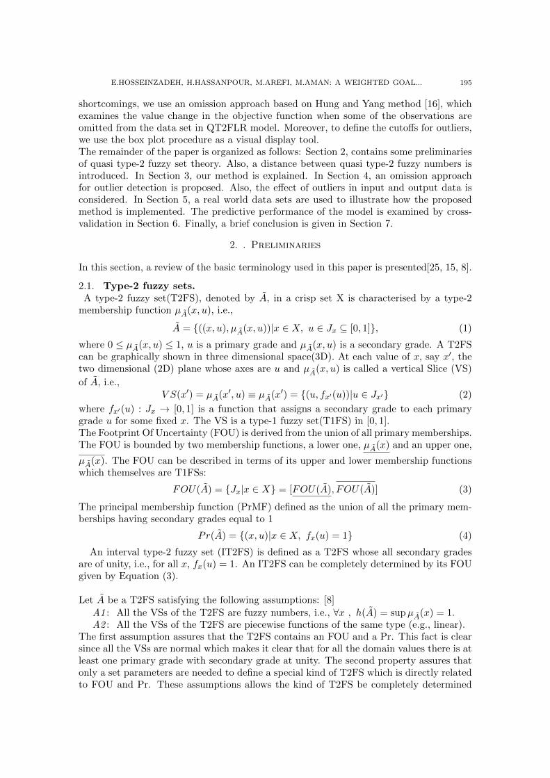
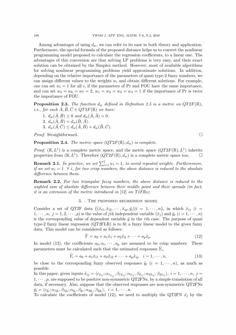
Definition 2.4. A QT2FN is called triangular if all of the membership functions FOU(A),

FOU(A), Pr(A) and vertical slices are triangular fuzzy numbers.

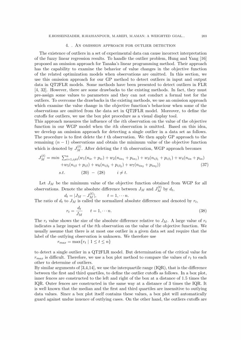
A triangular QT2FN, say A, is denoted by A = 〈c; l1, r1; l, r; l2, r2〉. The parameters used

here are Pr(A) = 〈c; l, r〉 and FOU(A) = 〈c; l1, r1; l2, r2〉 in which 〈c; l1, r1〉 = FOU(A)

and 〈c; l2, r2〉 = FOU(A).

Figure 1. (a) Non-symmetric triangular QT2FN; (b) Symmetric triangular QT2FN


A triangular QT2FN, say A can be denoted by its left and right spreads as follows:

A = 〈c;α1, β1;α, β;α2, β2〉

where α1 = c − l1, α = c − l, α2 = c − l2 and β1 = r1 − c, β = r − c, β2 = r2 − c arethe left and right spreads of FOU , Pr and FOU , respectively, and 0 ≤ α2 ≤ α ≤ α1,0 ≤ β2 ≤ β ≤ β1 (Fig 1 ). Specially, A is called symmetric if α1 = β1, α = β and α2 = β2.

In such a case A is denoted by A = 〈c;α1;α;α2〉.An ordinary triangular fuzzy number can be considered as a degenerated QT2FN in whichall of the spreads of FOU(A), FOU(A) and Pr(A) are equal and their secondary member-ship functions are zero. Also, a real number can be considered as a degenerated QT2FNwhose spreads and secondary membership functions are zero. The following formulas foraddition of two triangular QT2FNs and multiplication of a triangular QT2FN by a scalerare drawn from extension principle of zadeh [43].

Proposition 2.1. If A = 〈c;α1, β1;α, β;α2, β2〉 and B = 〈c′;α′1, β′1;α′, β′;α′2, β′2〉 be inQT2F (R) and λ ∈ R, then

A1 + A2 = 〈c+ c′;α1 + α′1, β1 + β′1;α+ α′, β + β′;α2 + α′2, β2 + β′2〉, (7)

λA1 =

{〈λc;λα1, λβ1;λα, λβ;λα2, λβ2〉 λ ≥ 0,〈λc;−λβ1,−λα1;−λβ,−λα;−λβ2,−λα2〉 λ < 0.

(8)

Proposition 2.2. Let r and s be two real numbers and A be a quasi type-2 fuzzy number.Then

(r + s)A ⊆ rA+ sA. (9)

Proof. According to Definition 2.2, Relation (9) is satisfied if and only if this relation is

satisfied for lower, principal and upper fuzzy numbers which define A. In other words

(r + s)A ⊆ rA+ sA⇐⇒ (r + s)A(x) ≤ rA(x) + sA(x), (10)

(r + s)A(x) ≤ rA(x) + sA(x),(r + s)A(x) ≤ rA(x) + sA(x).

However, the right hand side relations are hold for type-1 fuzzy numbers (see [12], Propo-sition 2.7), and the proof is complete. �

2.2. A distance between quasi type-2 fuzzy numbers.The observed data in our study are assumed to be QT2FN. So, we try to close the mem-

bership functions of observed and estimated responses from fuzzy linear regression modelby closing their corresponding parameters. Since QT2FNs are completely characterized bythe parameters of their FOU and Pr, closing the parameteres of two QTFNs is enough (infact necessary and sufficient) to close their membership functions, which is the purpose ofthis paper. To do this, based on the distance defined between two triangular fuzzy numbersby Hassanpour et al. [11], we propose the following weighted distance between QT2FNsin which different weights (wi) are used to show different importance of the parameters[15].

Definition 2.5. Let A = 〈c;α1, β1;α, β;α2, β2〉 and B = 〈c′;α′1, β′1;α′, β′;α′2, β′2〉 be in

QT2F (R) and wi > 0 for i = 1, · · · , 7. The distance between A and B as follows:

dw(A, B) = w1|α1 − α′1|+ w2|β1 − β′1|+ w3|α2 − α′2|+ w4|β2 − β′2|+w5|α− α′|+ w6|c− c′|+ w7|β − β′|. (11)


Among advantages of using dw, we can refer to its ease in both theory and application.Furthermore, the special formula of the proposed distance helps us to convert the nonlinearprogramming model proposed to calculate the regression coefficients, to a linear one. Theadvantages of this conversion are that solving LP problems is very easy, and their exactsolution can be obtained by the Simplex method. However, most of available algorithmsfor solving nonlinear programming problems yield approximate solutions. In addition,depending on the relative importance of the parameters of quasi type-2 fuzzy numbers, wecan assign different values to the weights wi and obtain different solutions. For example,one can set wi = 1 for all i, if the parameters of Pr and FOU have the same importance,and can set w5 = w6 = w7 = 2, w1 = w2 = w3 = w4 = 1 if the importance of Pr is twicethe importance of FOU.

Proposition 2.3. The function dw defined in Definition 2.5 is a metric on QT2F (R),

i.e., for each A, B, C ∈ QT2F (R) we have:

1. dw(A, B) ≥ 0 and dw(A, A) = 0.

2. dw(A, B) = dw(B, A).

3. dw(A, C) ≤ dw(A, B) + dw(B, C).

Proof. Straightforward. �

Proposition 2.4. The metric space (QT2F (R), dw) is complete.

Proof. (R, L1) is a complete metric space, and the metric space (QT2F (R), L1) inheritsproperties from (R, L1). Therefore (QT2F (R), dw) is a complete metric space too. �

Remark 2.1. In practice, we set∑7

i=1wi = 1, to avoid repeated weights. Furtheremore,if we set wi = 1 ∀ i, for two crisp numbers, the above distance is reduced to the absolutedifference between them.

Remark 2.2. For two triangular fuzzy numbers, the above distance is reduced to thewighted sum of absolute difference between their middle point and their spreads (in fact,it is an extension of the metric introduced in [12] on T1FRs).

3. . The proposed regression model

Consider a set of QT2F data {(xi1, xi2, · · · , xip, yi)|i = 1, · · · , n}, in which xij (i =1, · · · , n, j = 1, 2, · · · , p) is the value of j th independent variable (xj) and yi (i = 1, · · · , n)is the corresponding value of dependent variable y in the ith case. The purpose of quasitype-2 fuzzy linear regression (QT2FLR) is to fit a fuzzy linear model to the given fuzzydata. This model can be considered as follows:

Y = a0 + a1x1 + a2x2 + · · ·+ apxp. (12)

In model (12), the coefficients a0, a1, · · · , ap are assumed to be crisp numbers. These

parameters must be calculated such that the estimated responses Yi,

Yi = a0 + a1xi1 + a2xi2 + · · ·+ apxip i = 1, · · · , n, (13)

be close to the corresponding fuzzy observed responses yi (i = 1, · · · , n), as much aspossible.In this paper, given inputs xij = 〈cxij ;α1xij

, β1xij ;αxij , βxij ;α2xij , β2xij 〉, i = 1, · · · , n, j =

1, · · · , p, are supposed to be positive non-symmetric QT2FNs, by a simple translation of alldata, if necessary. Also, suppose that the observed responses are non-symmetric QT2FNsyi = 〈cyi ;α1yi , β1yi ;αyi , βyi ;α2yi , β2yi〉, i = 1, · · · , n.To calculate the coefficients of model (12), we need to multiply the QT2FN xj by the


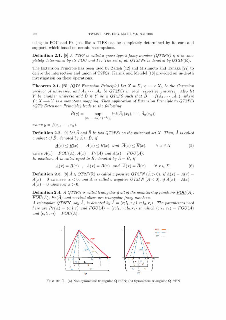
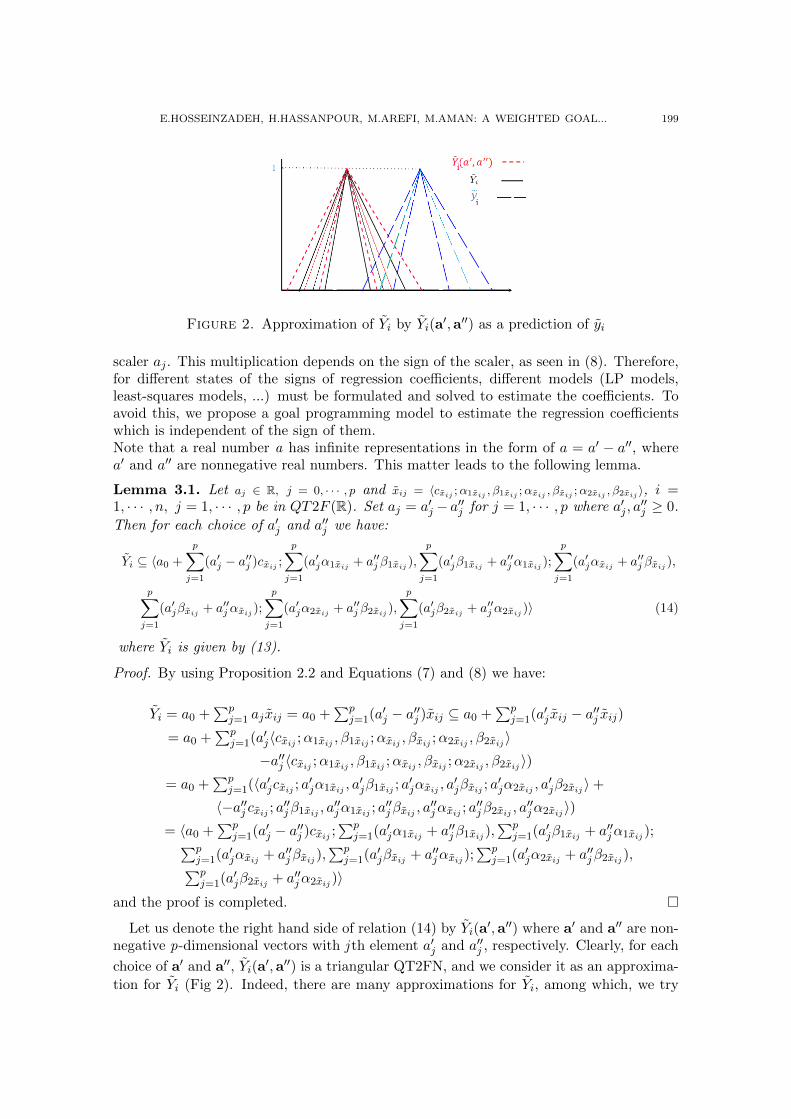
Figure 2. Approximation of Yi by Yi(a′,a′′) as a prediction of yi

scaler aj . This multiplication depends on the sign of the scaler, as seen in (8). Therefore,for different states of the signs of regression coefficients, different models (LP models,least-squares models, ...) must be formulated and solved to estimate the coefficients. Toavoid this, we propose a goal programming model to estimate the regression coefficientswhich is independent of the sign of them.Note that a real number a has infinite representations in the form of a = a′ − a′′, wherea′ and a′′ are nonnegative real numbers. This matter leads to the following lemma.

Lemma 3.1. Let aj ∈ R, j = 0, · · · , p and xij = 〈cxij ;α1xij , β1xij ;αxij , βxij ;α2xij , β2xij 〉, i =1, · · · , n, j = 1, · · · , p be in QT2F (R). Set aj = a′j − a′′j for j = 1, · · · , p where a′j , a

′′j ≥ 0.

Then for each choice of a′j and a′′j we have:

Yi ⊆ 〈a0 +

p∑j=1

(a′j − a′′j )cxij;

p∑j=1

(a′jα1xij+ a′′j β1xij

),

p∑j=1

(a′jβ1xij+ a′′jα1xij

);

p∑j=1

(a′jαxij+ a′′j βxij

),

p∑j=1

(a′jβxij+ a′′jαxij

);

p∑j=1

(a′jα2xij+ a′′j β2xij

),

p∑j=1

(a′jβ2xij+ a′′jα2xij

)〉 (14)

where Yi is given by (13).

Proof. By using Proposition 2.2 and Equations (7) and (8) we have:

Yi = a0 +∑p

j=1 aj xij = a0 +∑p

j=1(a′j − a′′j )xij ⊆ a0 +

∑pj=1(a

′j xij − a′′j xij)

= a0 +∑p

j=1(a′j〈cxij ;α1xij , β1xij ;αxij , βxij ;α2xij , β2xij 〉−a′′j 〈cxij ;α1xij , β1xij ;αxij , βxij ;α2xij , β2xij 〉)

= a0 +∑p

j=1(〈a′jcxij ; a′jα1xij , a′jβ1xij ; a

′jαxij , a

′jβxij ; a

′jα2xij , a

′jβ2xij 〉+

〈−a′′j cxij ; a′′jβ1xij , a′′jα1xij ; a′′jβxij , a

′′jαxij ; a

′′jβ2xij , a

′′jα2xij 〉)

= 〈a0 +∑p

j=1(a′j − a′′j )cxij ;

∑pj=1(a

′jα1xij + a′′jβ1xij ),

∑pj=1(a

′jβ1xij + a′′jα1xij );∑p

j=1(a′jαxij + a′′jβxij ),

∑pj=1(a

′jβxij + a′′jαxij );

∑pj=1(a

′jα2xij + a′′jβ2xij ),∑p

j=1(a′jβ2xij + a′′jα2xij )〉

and the proof is completed. �

Let us denote the right hand side of relation (14) by Yi(a′,a′′) where a′ and a′′ are non-

negative p-dimensional vectors with j th element a′j and a′′j , respectively. Clearly, for each

choice of a′ and a′′, Yi(a′,a′′) is a triangular QT2FN, and we consider it as an approxima-

tion for Yi (Fig 2). Indeed, there are many approximations for Yi, among which, we try


to choose the best approximation. We have to find Yi as close as possible to yi. Instead,first we approximate Yi to its supersets Yi(a

′,a′′) for different choices of a′ and a′′, as seen

in Lemma 3.1. Then, we try to find appropriate values of a′ and a′′ so that Yi(a′,a′′) be

close to yi as much as possible. To this end, we attempt to close the membership functionof each approximated response Yi(a

′,a′′) to that of corresponding observed response yias much as possible. Therefore, we introduce the following mathematical programmingproblem, which finds the best choices of a′ and a′′ for the coefficients of model (13):

minn∑i=1

dw(Yi(a′,a′′), yi)

s.t. a0 ∈ R, a′j , a′′j ≥ 0 j = 1, 2, · · · , p,

(15)

where d was introduced in Definition 2.5. The model (15) can be converted to a GP modelby choosing appropriate deviation variables. To this end, set

Yi(a′,a′′) = 〈cYi(a′,a′′);α1Yi(a′,a′′)

, β1Yi(a′,a′′);αYi(a′,a′′), βYi(a′,a′′);α2Yi(a′,a′′), β2Yi(a′,a′′)〉

for i = 1 · · ·n and define:

nik =1

2{|kYi(a′,a′′) − kyi | − (kYi(a′,a′′) − kyi)} (16)

pik =1

2{|kYi(a′,a′′) − kyi |+ (kYi(a′,a′′) − kyi)}, (17)

for k = c, α1, β1, α, β, α2, β2. In fact, nik and pik (k ∈ {c, α1, β1, α, β, α2, β2}) are thenegative and positive deviations between the parameters of the ith estimated and observedresponse, respectively. It can be easily seen that

niα1 =

{α1yi − α1Yi(a′,a′′)

α1Yi(a′,a′′)≤ α1yi ,

0 α1Yi(a′,a′′)> α1yi ,

(18)

piα1 =

{α1Yi(a′,a′′)

− α1yi α1yi ≤ α1Yi(a′,a′′),

0 α1yi > α1Yi(a′,a′′),

(19)

for i = 1 · · ·n. Similar relations are hold true for other deviation variables. By using theabove deviation variables, the model (15) converts to the following GP model:(WGP ) : min z =

∑ni=1(w1(nic + pic) +w2(niα1 + piα1) +w3(niβ1 + piβ1) +w4(niα + piα)

+ w5(niβ + piβ) + w6(niβ2 + piβ2) + w7(niα2 + piα2))

s.t.

p∑j=1

(a′jα1xij + a′′jβ1xij ) + niα1 − piα1 = α1yi i = 1, · · · , n (20)

p∑j=1

(a′jβ1xij + a′′jα1xij ) + niβ1 − piβ1 = β1yi i = 1, · · · , n (21)

p∑j=1

(a′jαxij + a′′jβxij ) + niα − piα = αyi i = 1, · · · , n (22)


p∑j=1

(a′jβxij + a′′jαxij ) + niβ − piβ = βyi i = 1, · · · , n (23)

p∑j=1

(a′jα2xij + a′′jβ2xij ) + niα2 − piα2 = α2yi i = 1, · · · , n (24)

p∑j=1

(a′jβ2xij + a′′jα2xij ) + niβ2 − piβ2 = β2yi i = 1, · · · , n (25)

nikpik = 0 i = 1, · · · , n, k = c, α1, β1, α, β, α2, β2 (26)

nik, pik ≥ 0 i = 1, · · · , n, k = c, α1, β1, α, β, α2, β2 (27)

a0 ∈ R , a′j , a′′j ≥ 0, j = 1, · · · , p. (28)

It is clear that if αyi = βyi for all i, we can set αxij = βxij for each i and j. Accordingly,the constraints (22) and (23) will be equivalent, and one of them (in fact n constraints)can be removed. Similarly, if α1yi = β1yi (α2yi = β2yi) for all i, we can set α1xij = β1xij(α1xij = β1xij ) for each i and j. Therefore, the constraints (20) and (21) ((24) and (25))will be be equivalent, and the constraints (21) ((25)) can be removed, then we obtain asmaller model. In addition, one can remove the constraints (26) and solve the obtained LPmodel by the Simplex method [1]. Another feature of WGP is that, it does not producenegative spreads for QT2FNs. This fact has been shown in the following proposition.

Proposition 3.1. The estimated responses from WGP have non-negative spreads.

Proof. The estimated responses from WGP are:Yi(a

′,a′′) = 〈cYi(a′,a′′);α1Yi(a′,a′′), β1Yi(a′,a′′);αYi(a′,a′′), βYi(a′,a′′);α2Yi(a′,a′′), β2Yi(a′,a′′)〉We have to show that kYi(a′,a′′) ≥ 0 for k ∈ {α1, β1, α, β, α2, β2}. According to the proof

of Lemma (3.1) we have:

α1Yi(a′,a′′)=∑p

j=1(a′jα1xij + a′′jβ1xij ) , β1Yi(a′,a′′) =

∑pj=1(a

′jβ1xij + a′′jα1xij )

αYi(a′,a′′) =∑p

j=1(a′jαxij + a′′jβxij ) , βYi(a′,a′′) =

∑pj=1(a

′jβxij + a′′jαxij )

α2Yi(a′,a′′)=∑p

j=1(a′jα2xij + a′′jβ2xij ) , β2Yi(a′,a′′) =

∑pj=1(a

′jβ2xij + a′′jα2xij )

which are all non-negative. Because a′j , a′′j , α1xij , β1xij , αxij , βxij , α2xij and β2xij are all

non-negative. �

Although the estimated responses Yi, i = 1, · · · , n have been approximated by Yi(a′,a′′),

i = 1, · · · , n, the following theorem shows that WGP yields the exact regression coefficientsand estimated responses if the given quasi type-2 fuzzy input-output data satisfy in a quasitype-2 fuzzy linear model.

Theorem 3.1. Suppose that the observed quasi type-2 fuzzy input-output data satisfy inthe quasi type-2 fuzzy linear model

y = a0 + a1x1 + a2x2 + · · ·+ apxp.Then:(i) The optimal solution of WGP contains a0, · · · , ap.(ii) The estimated responses from WGP and the observed responses are exactly the same

(i.e., Yi(a′,a′′) = yi).


Proof. (i). Set a0 = a0,

a′j =

{aj if aj ≥ 00 if aj < 0

and a′′j =

{0 if aj ≥ 0−aj if aj < 0

for j = 1, · · · , p, and nik = pik = 0, for i = 1, 2, · · · , n and k = c, α1, β1, α, β, α2, β2. First,we show that these values yield a feasible solution for WGP. Clearly, they satisfy in theconstraints (26)-(28). Without loss of generality, for simplicity, suppose that aj ≥ 0, j =1, · · · , p. By the assumption we have:

a0 +

p∑j=1

(a′j − a′′j )cxij + nic − pic = a0 +

p∑j=1

ajcxij = cyi , (29)

p∑j=1

(a′jα1xij + a′′jβ1xij ) + niα1 − piα1 =

p∑j=1

ajα1xij = α1yi , (30)

p∑j=1

(a′jβ1xij + a′′jα1xij ) + niβ1 − piβ1 =

p∑j=1

ajβ1xij = β1yi , (31)

p∑j=1

(a′jαxij + a′′jβxij ) + niα − piα =

p∑j=1

ajαxij = αyi (32)

p∑j=1

(a′jβxij + a′′jαxij ) + niβ − piβ =

p∑j=1

ajβxij = βyi (33)

p∑j=1

(a′jα2xij + a′′jβ2xij ) + niα2 − piα2 =

p∑j=1

ajα2xij = α2yi (34)

p∑j=1

(a′jβ2xij + a′′jα2xij ) + niβ2 − piβ2 =

p∑j=1

ajβ2xij = β2yi (35)

The Equations (29)-(35) show that the suggested values satisfy in the constraints (20)-(25). (i.e., we have a feasible solution for WGP). To show the optimality, note that theobjective function value of WGP for this feasible solution is 0, which is the least possi-ble value for a non-negative function. Therefore, the suggested values yield the optimalsolution of WGP. Indeed, in the optimal solution we have a′j − a′′j = aj .

(ii). The second part of the theorem immediately follows from (29)-(33). In fact, from(29)-(33) we have:

cYi(a′,a′′) = cyi , α1Yi

(a′,a′′) = α1yi , β1Yi(a′,a′′) = β1yi , αYi(a

′,a′′) = αyi

βYi(a′,a′′) = βyi , α2Yi

(a′,a′′) = α2yi , β2Yi(a′,a′′) = β2yi .

and the proof is completed. �

Remark 3.1. The explained method can be applied to QT2FLR with triangular IT2FNoutputs easily. Since, IT2FN completely determined using its FOU, it is enough to modifythe distance introduced in Definition 2.5 for two triangular IT2FN A = 〈c;α1, β1;α2, β2〉and B = 〈c′;α′1, β′1;α′2, β′2〉 as follows:

dw(A, B) = w1|c− c′|+ w2|α1 − α′1|+ w3|β1 − β′1|+ w4|α2 − α′2|+ w5|β2 − β′2|. (36)

In which w1, · · · , w5 > 0. The WGP model in this case is obtained from WGP by removingthe constraints (22) and (23).


4. . An omission approach for outlier detection

The existence of outliers in a set of experimental data can cause incorrect interpretationof the fuzzy linear regression results. To handle the outlier problem, Hung and Yang [16]proposed an omission approach for Tanaka’s linear programming method. Their approachhas the capability to examine the behavior of value changes in the objective functionof the related optimization models when observations are omitted. In this section, weuse this omission approach for our GP method to detect outliers in input and outputdata in QT2FLR models. Some methods have been presented to detect outliers in FLR[4, 32]. However, there are some drawbacks to the existing methods. In fact, they mustpre-assign some values to parameters and they can not conduct a formal test for theoutliers. To overcome the drawbacks in the existing methods, we use an omission approachwhich examine the value change in the objective function’s behaviour when some of theobservations are omitted from the data set in QT2FLR model. Moreover, to define thecutoffs for outliers, we use the box plot procedure as a visual display tool.This approach measures the influence of the ith observation on the value of the objectivefunction in our WGP model when the ith observation is omitted. Based on this idea,we develop an omission approach for detecting a single outlier in a data set as follows.The procedure is to first delete the t th observation. We then apply GP approach to theremaining (n − 1) observations and obtain the minimum value of the objective function

which is denoted by J(t)M . After deleting the t th observation, WGP approach becomes

J(t)M = min

∑ni=1,i 6=t(w1(nic + pic) + w2(niα1 + piα1) + w3(niβ1 + piβ1) + w4(niα + piα)

+w5(niβ + piβ) + w6(niβ2 + piβ2) + w7(niα2 + piα2)) (37)

s.t. (20) − (28) i 6= t.

Let JM be the minimum value of the objective function obtained from WGP for all

observations. Denote the absolute difference between JM and J(t)M by dt,

dt = |JM − J (t)M |, t = 1, · · ·n.

The ratio of dt to JM is called the normalized absolute difference and denoted by rt,

rt =dtJM

t = 1, · · ·n. (38)

The rt value shows the size of the absolute difference relative to JM . A large value of rtindicates a large impact of the tth observation on the value of the objective function. Weusually assume that there is at most one outlier in a given data set and require that thelabel of the outlying observation is unknown. We therefore use

rmax = max{rt | 1 ≤ t ≤ n}

to detect a single outlier in a QT2FLR model. But determination of the critical value forrmax is difficult. Therefore, we use a box plot method to compare the values of rt to eachother to determine of outliers.By similar arguments of [3,4,14], we use the interquartile range (IQR), that is the differencebetween the first and third quartiles, to define the outlier cutoffs as follows. In a box plot,inner fences are constructed to the left and right of the box at a distance of 1.5 times theIQR. Outer fences are constructed in the same way at a distance of 3 times the IQR. Itis well known that the median and the first and third quartiles are insensitive to outlyingdata values. Since a box plot itself contains these values, a box plot will automaticallyguard against undue inuence of outlying cases. On the other hand, the outliers cutoffs are


TABLE 1. Observed and predicted quasi type-2 fuzzy valued and their distance (for w = 1)i xi yi Yi dw

1 〈2; 1.25, 1.35, 0.5; 0.6, 0.25, 0.35〉〈4; 1.55, 1.5; 0.8, 0.75; 0.55, 0.5〉〈4.83; 1.22, 1.27; 0.50, 0.55; 0.26, 0.31〉 2.342 〈3.5; 1.59, 1.62; 0.84, 0.87; 0.59, 0.62〉〈5.5; 1.41, 1.55; 0.66, 0.8; 0.41, 0.55〉〈5.5; 1.53, 1.55; 0.81, 0.82; 0.57, 0.58〉 0.513 〈5.5; 1.45, 1.75; 0.7, 1; 0.45, 0.75〉〈7.5; 1.25, 1.75; 0.5, 1; 0.25, 0.75〉〈6.38; 1.47, 1.60; 0.75, 0.88; 0.51, 0.64〉 2.214 〈7; 1.75, 1.42; 1, 0.67; 0.75, 0.42〉〈6.5; 1.47, 1.28; 0.72, 0.53; 0.47, 0.28〉〈7.05; 1.59, 1.45; 0.87, 0.72; 0.63, 0.48〉 1.585 〈8.5; 1.45, 1.59; 0.7, 0.84; 0.45; 0.59〉〈8.5; 1.46, 1.39; 0.71, 0.64; 0.46, 0.39〉〈7.72; 1.43, 1.49; 0.70, 0.77; 0.46, 0.53〉 1.196 〈10.5; 1.56, 1.39; 0.81, 0.64; 0.56, 0.39〉〈8; 1.42, 1.4; 0.67, 0.65; 0.42, 0.4〉〈8.61; 1.45, 1.38; 0.73, 0.65; 0.49, 0.41〉 0.837 〈11; 1.32, 1.51; 0.57, 0.76; 0.32, 0.51〉〈10.5; 1.52, 1.57; 0.77, 0.82; 0.52, 0.57〉〈8.83; 1.31, 1.40; 0.59, 0.68; 0.35, 0.44〉 2.638 〈12.5; 1.44, 1.65; 0.69, 0.9; 0.44, 0.65 〈9.5; 1.75, 1.72; 1, 0.97; 0.75, 0.72〉〈9.5; 1.43, 1.53; 0.71, 0.81; 0.47, 0.57〉 1.36

Mean of distance 1.58

determined by the first and third quartiles.They can dampen the inuence of even a singlewild data value. Therefore, we use a box plot to determine whether rmax is an outlier ornot. The data points that lie between the inner and outer fences are denoted by a circle”◦” called mild outliers. The data points that lie beyond the outer fences are denoted byan asterisk ”∗”, called extreme outliers.

4.1. . Cross validation. To further investigation of the performance of the model, weapply an index based on the cross validation method [40] to examine the predictive abilityof the models. To this end, each time, the ith observation is left out from the data set, whilethe remaining observations are used to develop a quasi type-2 fuzzy regression model. Thenthe obtained model is used to predict the response value of the i th observation (denoted

by Y(−i)(xi)). Finally, to compare the i th observed response yi and the predicted value

Y(−i)(xi), we calculate the mean of distances dw (Eq. 2.5) between yi and Y(−i)(xi) whichwe call it MDC.

Definition 4.1. For QT2F regression model (12), the MDC index is defined by

MDC =1

n

n∑i=1

dw(Y(−i)(xi), yi), (39)

where Y(−i)(xi) is the QT2F response predicted by omitting the ith observation or the ithinput-output data.

Definition 4.2. For QT2F regression model (15), the mean of distances between estimatedand observed values is defined by

MD∗ =1

n

n∑i=1

dw(Yi, yi) (40)

Now, by using the above indices, the relative error of the estimated responses can bedefined as

RE =|MDC −MD∗|

MD∗. (41)

5. . Numerical Results

Since examples containing quasi type-2 fuzzy data did not exist in previous works (notethat almost all of the previous studies concenterated on type-1 fuzzy data), we change thedata of examples given in [28, 12] to non-symmetric triangular QT2FNs.

Example 5.1. This example considers 8 non-symmetric quasi type-2 fuzzy input-outputdata. The observed inputs and responses are given in Table 1. The regression model ob-tained by solving LP model related to WGP for the data of Table 1 with w1 = w2 = · · · =w7 = 1 is as follows:

Y = 3.9444 + 0.4444x.


An outlier may be outlying with respect to its spreads, its center, or both. In thefollowing example, we consider different cases to see the effect of outliers on our results.

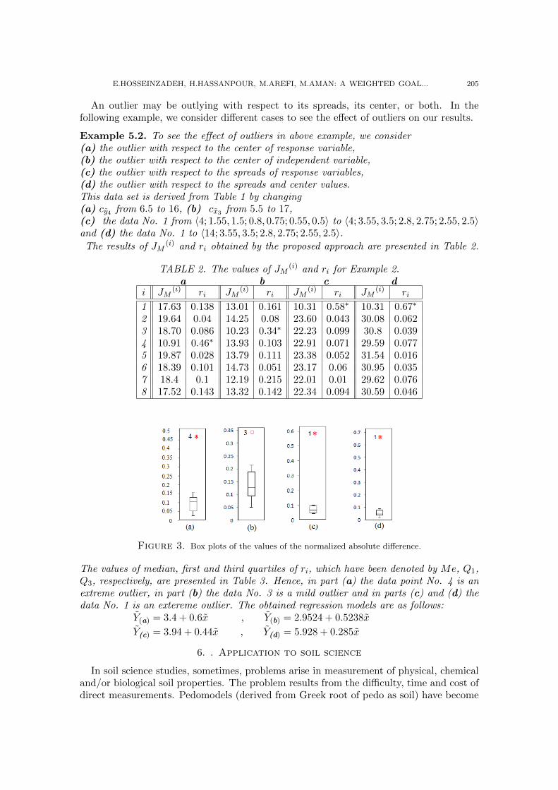
Example 5.2. To see the effect of outliers in above example, we consider(a) the outlier with respect to the center of response variable,(b) the outlier with respect to the center of independent variable,(c) the outlier with respect to the spreads of response variables,(d) the outlier with respect to the spreads and center values.This data set is derived from Table 1 by changing(a) cy4 from 6.5 to 16, (b) cx3 from 5.5 to 17,(c) the data No. 1 from 〈4; 1.55, 1.5; 0.8, 0.75; 0.55, 0.5〉 to 〈4; 3.55, 3.5; 2.8, 2.75; 2.55, 2.5〉and (d) the data No. 1 to 〈14; 3.55, 3.5; 2.8, 2.75; 2.55, 2.5〉.

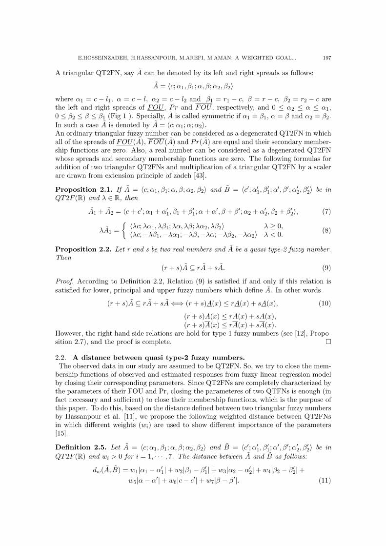
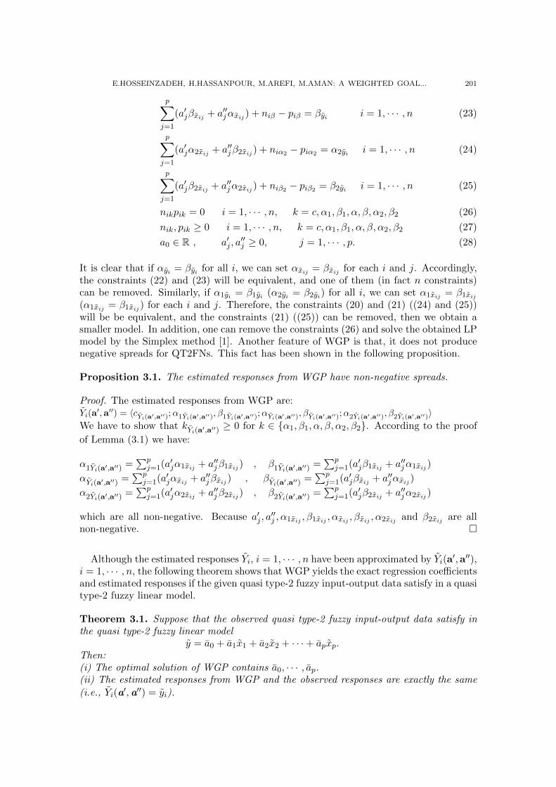
The results of JM(i) and ri obtained by the proposed approach are presented in Table 2.

TABLE 2. The values of JM(i) and ri for Example 2.

a b c di JM

(i) ri JM(i) ri JM

(i) ri JM(i) ri

1 17.63 0.138 13.01 0.161 10.31 0.58∗ 10.31 0.67∗

2 19.64 0.04 14.25 0.08 23.60 0.043 30.08 0.0623 18.70 0.086 10.23 0.34∗ 22.23 0.099 30.8 0.0394 10.91 0.46∗ 13.93 0.103 22.91 0.071 29.59 0.0775 19.87 0.028 13.79 0.111 23.38 0.052 31.54 0.0166 18.39 0.101 14.73 0.051 23.17 0.06 30.95 0.0357 18.4 0.1 12.19 0.215 22.01 0.01 29.62 0.0768 17.52 0.143 13.32 0.142 22.34 0.094 30.59 0.046

Figure 3. Box plots of the values of the normalized absolute difference.

The values of median, first and third quartiles of ri, which have been denoted by Me, Q1,Q3, respectively, are presented in Table 3. Hence, in part (a) the data point No. 4 is anextreme outlier, in part (b) the data No. 3 is a mild outlier and in parts (c) and (d) thedata No. 1 is an extereme outlier. The obtained regression models are as follows:

Y(a) = 3.4 + 0.6x , Y(b) = 2.9524 + 0.5238x

Y(c) = 3.94 + 0.44x , Y(d) = 5.928 + 0.285x

6. . Application to soil science

In soil science studies, sometimes, problems arise in measurement of physical, chemicaland/or biological soil properties. The problem results from the difficulty, time and cost ofdirect measurements. Pedomodels (derived from Greek root of pedo as soil) have become


TABLE 3. The values of Me, Q1, Q3, IQR and cutoffs for Table 2

(a) (b) (c) (d)

Me 0.1005 0.126 0.065 0.054Q1 0.06 0.091 0.047 0.037Q3 0.14 0.185 0.096 0.076IQR 0.04 0.094 0.049 0.039

Q1 − 1.5IQR 0.003 -0.049 -0.02 -0.02Q1 − 3IQR -0.057 -0.189 -0.1 -0.08Q3 + 1.5IQR 0.2 0.32 0.169 0.134Q3 + 3QR 0.26 0.46 0.243 0.193

a popular topic in soil science and environmental research. They are predictive functionsof certain soil properties based on other easily or cheaply measured properties [31]. Inthis article, two pedomodels including one and two independent variables are studied todevelop the relationships between different chemical and physical soil properties by meansof quasi type-2 fuzzy regression technique. Based on a study in a part of Silakhor plain(situated in a province located in the west of Iran), a total of 24 core samples were obtainedfrom 0.0 to 25− cm depth [29].

Table 4. Observed and predicted quasi type-2 fuzzy values of SAR-ESP and their distances (for w = 1)

i SAR (xi) ESP (yi) Predicted ESP (Yi) dw

1 〈0.78; 0.78, 0.55; 0.39, 0.43; 0.01, 0.32〉〈3.08; 3.06, 2.92; 1.55, 2.37; 0.04, 1.82〉〈5.58; 5.47, 4.3; 2.95, 3.15; 0.42, 2〉 9.06

2 〈0.64; 0.57, 0.24; 0.31, 0.17; 0.06, 0.11〉〈2.86; 2.55, 2.03; 1.40, 1.93; 0.26, 1.83〉〈4.87; 3.81, 2.13; 2.15, 1.44; 0.49, 0.75〉 5.94

3 〈0.62; 0.57, 0.22; 0.32, 0.21; 0.07, 0.2〉〈6.25; 5.74, 3.6; 3.23, 2.37; 0.72, 1.14〉〈4.77; 3.79, 2.01; 2.22, 1.66; 0.66, 1.32〉 6.94

4 〈0.49; 0.38, 0.14; 0.27, 0.1; 0.16, 0.07〉〈4.11; 3.17, 3.81; 2.24, 2.74; 1.32, 1.67〉〈4.11; 2.52, 1.3; 1.79, 0.95; 1.07, 0.61〉 6.67

5 〈1.1; 0.83, 0.52; 0.64, 0.42; 0.45, 0.32〉〈1.04; 0.78, 1.01; 0.6, 0.71; 0.43, 0.42〉〈7.21; 5.75, 4.17; 4.45, 3.33; 3.16, 2.5〉 25.61

6 〈0.61; 0.36, 0.36; 0.31, 0.19; 0.26, 0.02〉〈2.71; 1.62, 2.43; 1.39, 1.58; 1.17, 0.73〉〈4.72; 2.64, 2.64; 2.14, 1.53; 1.64, 0.41〉 4.83

7 〈0.74; 0.31, 0.25; 0.25, 0.23; 0.2, 0.22〉〈4.45; 1.87, 1.9; 1.54, 1.16; 1.22, 0.43〉〈5.38; 2.21, 1.9; 1.85, 1.75; 1.49, 1.59〉 3.61

8 〈1.15; 0.64, 1.05; 0.53, 0.76; 0.42, 0.47〉〈6.92; 3.86, 4.31; 3.2, 3.43; 2.54, 2.55〉〈7.47; 5.17, 7.26; 4.15, 5.33; 3.14, 3.4〉 9.13

9 〈1.08; 0.87, 0.91; 0.59, 0.64; 0.32, 0.38〉〈7.41; 6, 1.63; 4.09, 1.4; 2.18, 1.17〉〈7.11; 6.44, 6.64; 4.43, 4.68; 2.42, 2.72〉 11.19

10 〈0.38; 0.37, 0.16; 0.2, 0.12; 0.03, 0.08〉〈9.08; 8.74, 9.03; 4.68, 8.13; 0.63, 7.23〉〈3.55; 2.48, 1.41; 1.38, 0.97; 0.27, 0.53〉 36.91

11 〈0.61; 0.58, 0.24; 0.31, 0.2; 0.04, 0.16〉〈6.56; 6.19, 3.45; 3.33, 3.26; 0.47, 3.08〉〈4.72; 3.88, 2.15; 2.15, 1.59; 0.43, 1.04〉 10.36

12 〈0.98; 0.62, 0.25; 0.4, 0.14; 0.18, 0.03〉〈5.05; 3.17, 3.24; 2.06, 2.86; 0.95, 2.48〉〈6.6; 4.14, 2.25; 2.64, 1.32; 1.15, 0.39〉 7.92

13 〈0.71; 0.62, 0.61; 0.59, 0.59; 0.57, 0.58〉〈5.23; 4.55, 4.1; 4.35, 2.27; 4.16, 0.44〉〈5.23; 4.55, 4.49; 4.37, 4.37; 4.2, 4.25〉 6.38

14 〈0.5; 0.44, 0.37; 0.35, 0.355; 0.26, 0.34〉〈5.16; 4.59, 2.35; 3.63, 1.66; 2.67, 0.98〉〈4.16; 3.15, 2.8; 2.58, 2.6; 2, 2.41〉 6.97

15 〈0.77; 0.4, 0.59; 0.27, 0.49; 0.14, 0.39〉〈11.1; 5.84, 10.57; 3.9, 7.18; 1.97, 3.79〉〈5.53; 3.15, 4.12; 2.23, 3.35; 1.31, 2.58〉 22.04

16 〈0.99; 0.7, 0.78; 0.44, 0.58; 0.19, 0.39〉〈4.47; 3.16, 0.86; 2, 0.55; 0.85, 0.24〉〈6.65; 5.24, 5.64; 3.43, 4.14; 1.62, 2.64〉 17.25

17 〈3.6; 3.42, 2.17; 2.84, 1.72; 2.27, 1.28〉〈28.84; 27.5, 24.56; 22.8, 23; 18.13, 21.7〉〈19.9; 23.74, 17.4; 19.6, 13.9; 15.6, 10.5〉 45.84

18 〈0.86; 0.57, 0.4; 0.29, 0.31; 0.02, 0.22〉〈9.43; 6.28, 7.75; 3.24, 5.06; 0.2, 2.37〉〈5.99; 4, 3.13; 2.18, 2.26; 0.37, 1.39〉 15.33

19 〈0.61; 0.37, 0.47; 0.31, 0.27; 0.26, 0.07〉〈4.5; 2.7, 2.31; 2.3, 1.75; 1.9, 1.2〉〈4.72; 2.83, 3.34; 2.26, 2.03; 1.69, 0.73〉 2.37

20 〈0.64; 0.4, 0.48; 0.37, 0.38; 0.34, 0.28〉〈9.3; 5.79, 8.81; 5.35, 4.56; 4.91, 0.31〉〈4.87; 3.03, 3.44; 2.73, 2.78; 2.43, 2.12〉 21.23

21 〈0.71; 0.65, 0.47; 0.48, 0.425; 0.32, 0.38〉〈9.48; 8.7, 7.68; 6.5, 4.88; 4.31, 2.09〉〈5.23; 4.57, 3.66; 3.5, 3.19; 2.42, 2.72〉 19.61

22 〈0.61; 0.47, 0.19; 0.27, 0.15; 0.08, 0.11〉〈3.65; 2.83, 1.03; 1.66, 1.01; 0.49, 0.99〉〈4.72; 3.14, 1.71; 1.88, 1.24; 0.62, 0.77〉 2.87

23 〈0.63; 0.14, 0.19; 0.09, 0.19; 0.04, 0.19〉〈10.14; 2.27, 9.35; 1.49, 7.22; 0.71, 5.09〉〈4.82; 1.08, 1.34; 0.77, 1.28; 0.46, 1.22〉 25.26

24 〈1.13; 0.99, 0.99; 0.63, 0.57; 0.28, 0.16〉〈3; 2.64, 2.45; 1.69, 2.28; 0.75, 2.12〉〈7.36; 7.28, 7.28; 4.6, 4.29; 1.92, 1.31〉 20.74


6.1. . Pedomodel of ESP-SAR.. We first wish to provide a relationship betweenexchangeable sodium percentage (ESP), as the dependent variable, and sodium absorptionratio (SAR), as an independent variable. The exchange sodium percentage, ESP, governsthe source/sink phenomenon for ionic constituents, i.e., sodium, as a contaminant in sodicsoils, is calculated from the ratio of exchangeable sodium, Nax, to cation exchangeablecapacity, CEC. All these soil parameters, measured on soil colloidal surface, are time


consuming and costly. Due to close relationship between the distribution of cations inthe exchange and solution phases, it is preferred to estimate ESP from sodium absorptionratio, SAR, in soil solution [29]. In this case, ESP is considered as cost and time variable,therefore the need for less expensive indirect measurement is emphasized. Measurementsof SAR have been related to ESP due to low cost, simplicity, and the possibility of relatingmeasurements to the quantity and quality parameters. But, due to some impreciseness inrelated experimental environment, the observations of response variable (ESP) are givenin fuzzy form. Thus, we may use a fuzzy method for modeling such a data set [29].

Estimation of model parameters. To develop a relationship between ESP (as a depen-dent variable) and SAR (as an independent variable), using quasi type-2 fuzzy regression,first, the values of dependent variable yi and independent variables xij , were fuzzified byconsulting an expert using asymmetric triangular QT2FN with right and left spreads pro-portional to yi and xij , respectively. The results are given in Table 4. These amounts ofvagueness were based on expert opinion and might be considered as the acceptable levelsof uncertainty.In this study, for each choice of a′1 and a′′1, the regression model for the data of table 4 isas follows:

Y = a0 + a1x1 = a0 + (a′1 − a′′1)x1 (42)

In the above model, non-symmetric QT2FNs Y and x1 are cation sodium absorption ratio(SAR) and exchange sodium percentage (ESP), respectively.According to the proposed method, the regression model is obtained as

Y = a0 + (a′1 − a′′1)x1 = 1.61 + (6.22− 1.13)x1 =

〈1.61 + 5.09cx1; 6.22α1x1 + 1.13β1x1, 6.22β1x1 + 1.13α1x1; 6.22αx1 + 1.13βx1,

6.22βx1 + 1.13αx1; 6.22α2x1 + 1.13β2x1, 6.22β2x1 + 1.13α2x1〉 (43)

The above QT2F regression model can be used to predict the ESP of a new case. Forexample, if for a new case, SAR = 〈1.08; 0.87, 0.91; 0.59, 0.64; 0.32, 0.38〉 then by Eq. (43),

we predict the ESP as Y = 〈7.10; 6.43, 6.64; 4.38, 4.64; 2.41, 2.72〉.

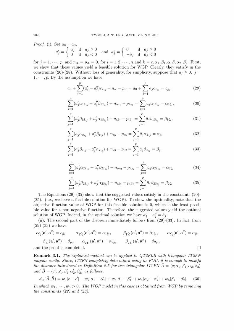
6.2. . Pedomodel of CEC-SAND-OM.. The second model provides a relationshipbetween cation exchange capacity (CEC), as a function of two soil variables namely per-centage of sand content (SAND) and organic matter content (OM)(Table 5). In the soil,organic matter can enhance the CEC, while the sand content has negative effect on thecation exchange capacity [29].

Estimation of model parameters. The regression model for the data of Table 5 is asfollows:

Y = a0 + a1x1 + a2x2 (44)

where for each choice of a′j and a′′j , j = 1, 2 Eq. (44) is obtained as following

Y = a0 + (a′1 − a′′1)x1 + (a′2 − a′′2)x2 (45)

In the above model, non-symmetric QT2FNs Y , x1 and x2 are cation exchange capacity(CEC), percentage of sand content (SAND) and organic matter content (OM), respectively.By solving the linear programming problem related to WGP, the regression model isobtained as

Y = a0 + (a′1 − a′′1)x1 + (a′2 − a′′2)x2 = 22.19 + (0.02− 0.19)x1 + (4.23− 2.67)x2

= 22.19 + (−0.17)x1 + (1.56)x2 (46)


TABLE 6. Values of the independent variable (x), the dependent variable (y) and the corresponding predictions of Y by

cross-validation method and the distances between the observed and estimated values(for w = 1)

i xi yi Yi dw1 〈2; 1.25, 1.35, 0.5; 0.6, 0.25, 0.35〉〈4; 1.55, 1.5; 0.8, 0.75; 0.55, 0.5〉〈4.8, 1.2, 1.25, 0.49, 0.54, 0.26, 0.3〉 2.42

2 〈3.5; 1.59, 1.62; 0.84, 0.87; 0.59, 0.62〉〈5.5; 1.41, 1.55; 0.66, 0.8; 0.41, 0.55〉〈4.78, 1.57, 1.58, 0.83, 0.84, 0.58, 0.6〉 1.37

3 〈5.5; 1.45, 1.75; 0.7, 1; 0.45, 0.75〉〈7.5; 1.25, 1.75; 0.5, 1; 0.25, 0.75〉〈5.83, 1.45, 1.61, 0.73, 0.89, 0.49, 0.65〉 2.69

4 〈7; 1.75, 1.42; 1, 0.67; 0.75, 0.42〉〈6.5; 1.47, 1.28; 0.72, 0.53; 0.47, 0.28〉〈7.6, 1.66, 1.46, 0.92, 0.72, 0.67, 0.47〉 2.28

5 〈8.5; 1.45, 1.59; 0.7, 0.84; 0.45; 0.59〉〈8.5; 1.46, 1.39; 0.71, 0.64; 0.46, 0.39〉〈7.4, 1.45, 1.52, 0.71, 0.79, 0.47, 0.54〉 1.56

6 〈10.5; 1.56, 1.39; 0.81, 0.64; 0.56, 0.39〉〈8; 1.42, 1.4; 0.67, 0.65; 0.42, 0.4〉〈9.7, 1.5, 1.4, 0.76, 0.66, 0.52, 0.41〉 2.02

7 〈11; 1.32, 1.51; 0.57, 0.76; 0.32, 0.51〉〈10.5; 1.52, 1.57; 0.77, 0.82; 0.52, 0.57〉〈8.83, 1.29, 1.37, 0.58, 0.67, 0.34, 0.43〉 2.72

8 〈12.5; 1.44, 1.65; 0.69, 0.9; 0.44, 0.65 〈9.5; 1.75, 1.72; 1, 0.97; 0.75, 0.72〉〈11.26, 1.4, 1.55, 0.68, 0.83, 0.45, 0.59〉 3.14


The above QT2F regression model can be used to predict the CEC of a new case. Forexample, if for a new case,

SAND = 〈38; 36.2, 17.29; 30.04, 12.26; 23.88, 7.24〉OM = 〈0.84; 0.24, 0.35; 0.235, 0.29; 0.23, 0.23〉

then by Eq. (46), the predicted CEC is

Y = 〈17.04; 6.035, 9.33; 4.66, 7.78; 3.42, 6.25〉.

In order to evaluate the predictive ability of the above models, the MDC is calculated foreach model. For example, the results of example 5.1 are given in Table 6. In this examplethe value of MDC was obtained to be 2.27 and the value of MD∗ is 1.57, which the relativediffrence between them is equal to 0.3.

• The value of the MDC for the ESP-SAR regression was obtained to be 16.92, whichis very close to the value of MD∗, i.e., 14.34. Note that the relative error betweenMDC and MD∗ is RE=0.15.• The value of the MDC for the CEC-OM-SAND regression was obtained to be 27.9,

which is close to the value of MD∗, i.e., 27.21. Note that the relative error betweenMDC and MD∗ is RE=0.02.

It is appeared that predictive ability to the SAND-OM-CEC model is much better thanthe ESP-SAR model.Recently, Rabiei et al. [34] used a distance on the space of interval type-2 fuzzy numbers(which determinated using its FOU) and proposed a least-squares method (LS) to obtaincoefficients of the proposed model. In soil science examples, if input and output variablesare considered to be interval-valued fuzzy numbers, we use the distance introduced in(36). In the case of interval type-2 fuzzy input-output data, the regression models and therelative error between MDC and MD∗ in two approachs are as follows:

• ESP-SAR regression model:YGP = 1.172 + 5.742x , YLS = 0.835 + 6.879xrelative error between MDC and MD∗ for GP model= 0.129relative error between MDC and MD∗ for LS model= 0.273

• SAND-OM-CEC regression model:YGP = 21.96− 0.16x1 + 1.57x2 , YLS = 21.97− 0.23x1 + 2.57x2.relative error between MDC and MD∗ for GP model= 0.04relative error between MDC and MD∗ for LS model= 0.09

Since, the relative error between MDC and MD∗ for GP model are less than LS model,the predictive ability of our model is much better than LS model in these examples.


Tab

le5.

Ob

serv

edan

dp

red

icte

dqu

asi

typ

e-2

fuzz

yva

lues

ofS

AN

D,

OM

and

CE

C(f

orw

=1)

iSA

ND

(xi1

)O

M(x

i2)

CE

C(y

i)

Pre

dic

ted

CE

C(Y

i)

dw

1〈35;2

6.44,3

3.34;2

0.9,2

7.67;1

5.36,2

2〉〈0.88;0.84,0.37;0.68,0.27;0.52,0.18〉

〈16.5;1

1.54,1

6.4;9.2,8.31;6.87,0.23〉

〈17.59;1

1.54,9.62;9.39,7.6;7.25,5.58〉

14.5

2〈37;2

4.31,2

4.62;2

1.99,1

2.7;1

9.68,0.78〉〈1.13;0.8,0.44;0.76,0.36;0.72,0.29〉

〈18.6;6.91,1

6.61;5.1,9.14;3.3,1.68〉

〈17.64;9.83,9.21;7.11,8.08;4.4,6.95〉

20.7

23〈27;8.59,1

6.19;6.7,1

3.8;4.81,1

1.41〉

〈1.31;0.75,0.34;0.49,0.19;0.24,0.04〉

〈19.3;6.73,1

7.74;6.41,9.97;6.09,2.2〉

〈19.63;7.38,5.45;5.4,3.71;3.42,1.98〉

23.4

14〈29;8.96,1

8.05;8.8,1

6.67;8.64,1

5.3〉

〈1.98;1.83,1.7;1.32,1.65;0.81,1.61〉

〈20.3;5.88,1

5.65;4.5,1

1.09;3.1,6.53〉

〈20.33;1

5.93,1

4.16;1

3.4,1

2.6;1

0.86,1

1〉

34.1

85〈38;3

3.2,3

4.87;1

9.31,2

6.07;5.42,1

7.28〉〈1.02;0.99,0.75;0.7,0.72;0.41,0.7〉

〈17.3;8.13,1

3;6.58,1

0.05;5.03,7.11〉

〈17.3;1

3.63,1

2.97;1

0.34,9.22;7.05,5.47〉

13.7

56〈32;3

1.81,2

4.78;1

6.13,1

4.53;0.45,4.29〉〈1.29;1.16,1

;0.75,0.82;0.35,0.65〉

〈20.4;1

2.13,1

2.21;6.45,1

0.52;0.77,8.84〉〈18.74;1

3.04,1

3.99;8.55,8.93;4.05,3.86〉

16.3

17〈29;2

5.9,6.49;1

4.25,4.25;2.61,2.02〉

〈1.52;0.65,1.19;0.4,0.89;0.15,0.6〉

〈19.3;6.5,8.1;6.08,6.7;5.66,5.31〉

〈19.61;7.74,1

1.9;5.21,7.69;2.68,3.48〉

12.0

28〈18;1

6.54,1

5.82;9.3,1

0.15;2.06,4.48〉〈1.33;0.83,0.82;0.66,0.65;0.49,0.49〉

〈21.9;1

9.94,1

2.2;1

4.42,1

0.12;8.91,8.05〉〈21.19;9.11,9.21;6.7,6.54;4.29,3.87〉

34.5

99〈40;3

0.84,3

7.97;2

1.85,3

0.8;1

2.87,2

3.7〉〈1.71;0.38,0.8;0.32,0.62;0.27,0.44〉

〈15.9;1

3.43,1

2.87;9.54,8.77;5.66,4.68〉〈18.03;1

1.72,1

1.16;9.44,8.37;7.16,5.57〉

8.4

410〈28;2

1.02,1

9.84;1

6.26,1

8.88;1

1.5,1

7.92〉〈2;2,1.54;1.79,0.88;1.59,0.23〉

〈18.3;7.72,1

7.61;5.7,9.43;3.71,1.26〉

〈20.53;1

6.81,1

6.31;1

3.93,1

2.07;1

1.04,7.8〉

37.3

911〈13;7.78,7.48;6.7,4.92;5.63,2.37〉

〈1.68;0.88,1.27;0.83,1

;0.79,0.74〉

〈22.6;8.73,2

1.33;7.26,1

1.47;5.79,1.62〉〈22.6;8.73,9.39;7.31,7.88;5.9,6.38〉

20.4

512〈19;7.98,1

7.59;6.6,1

2.66;5.23,7.74〉

〈2.15;1.38,1.41;1.215,1.27;1.05,1.14〉〈23.7;6.08,1

4.89;3.44,9.67;0.8,4.46〉

〈22.3;1

3.17,1

1.57;1

1.13,1

0.19;9.09,8.8〉

32.6

513〈31;1

7.27,3

0.22;1

4.3,2

1.31;1

1.4,1

2.41〉〈3.52;2.76,1.12;1.53,0.87;0.3,0.63〉

〈22.4;1

8.82,2

3.21;1

8.3,2

2.32;1

7.8,2

1.43〉〈22.4;2

0.87,1

6.1;1

3.23,1

1.01;5.6,5.93〉

53.2

714〈31;2

5.1,2

7.7;1

7.11,1

8.06;9.13,8.3〉

〈2.33;1.06,0.72;0.75,0.7;0.44,0.69〉

〈21.8;1

6.04,1

9.4;1

5.5,1

5.3;1

4.98,1

1.28〉〈20.54;1

2.3,1

1.31;8.9,8.67;5.5,6.03〉

41.0

315〈17;1

6.36,7.24;8.76,4.44;1.17,1.64〉

〈1.71;1.63,1.49;1.105,0.86;0.58,0.24〉〈23.8;1

8.4,1

2.52;1

5.16,8.36;1

1.95,4.21〉〈21.96;1

2.63,1

3.97;8.03,8.4;3.43,2.82〉

26.0

916〈14;1

3.21,8.71;7.1,6.93;1,5.16〉

〈1.14;0.22,1.13;0.14,0.57;0.06,0.02〉

〈20.8;1

6.32,1

4.68;1

2.265,9.3;8.21,3.93〉〈21.58;5.91,8.1;3.61,4.32;1.32,0.54〉

41.6

517〈19;1

1.94,4.18;7.75,3.58;3.57,2.99〉

〈0.99;0.84,0.88;0.79,0.48;0.74,0.09〉

〈17.5;1

0.83,1

6.67;8.63,1

3.83;6.43,1

1〉〈20.49;6.97,8.36;5.5,5.73;4.02,3.11〉

36.6

818〈28;2

4.34,2

7.85;2

3.31,2

5.1;2

2.3,2

2.31〉〈1.14;0.94,1.05;0.61,0.59;0.3,0.13〉

〈17.8;8.34,1

1.85;6.44,6.11;4.55,0.38〉〈19.19;1

2.67,1

2.25;9.51,9.17;6.35,6.1〉

19.7

919〈26;2

3.13,1

3.66;1

8.3,1

2.94;1

3.45,1

2.2〉〈1.46;0.75,1.13;0.57,0.8;0.39,0.47〉

〈20.2;1

5.6,1

2.11;8.98,1

0.32;2.37,8.54〉〈20.03;9.32,1

1.53;7.44,8.71;5.55,5.9〉

15.9

920〈32;1

6.83,2

0.52;1

1.25,1

8.1;5.67,1

5.7〉〈1.81;1.71,1.36;0.88,1.05;0.06,0.74〉

〈20;1

5.11,1

2.45;1

1.94,1

1.5;8.78,1

0.55〉〈19.55;1

5.19,1

4.01;1

0.28,9.37;5.37,4.72〉

15.1

21〈10;7.06,7.83;4.47,4.33;1.89,0.84〉

〈1.38;1.12,0.83;0.71,0.71;0.3,0.6〉

〈22.8;1

5,2

0.92;1

3.55,1

5.64;1

2.13,1

0.37〉〈22.64;8.62,8.03;5.84,5.88;3.07,3.72〉

52.5

622〈38;3

6.2,1

7.29;3

0.04,1

2.26;2

3.88,7.24〉〈0.84;0.24,0.35;0.23,0.29;0.23,0.23〉

〈19.1;6.08,1

4.79;4.74,8.67;3.4,2.56〉

〈17.01;6.06,9.46;4.78,7.9;3.5,6.34〉

12.1

123〈49;3

2.6,4

6.67;1

6.82,3

1.69;1.04,1

6.72〉〈1.48;1.36,0.82;1.05,0.68;0.74,0.54〉

〈12.1;3.74,2.71;3.67,1.77;3.6,0.84〉

〈16.14;1

7.64,1

4.4;1

2.73,9.61;7.81,4.82〉

54.7

424〈42;2

5.19,8.09;2

1.47,5.18;1

7.75,2.28〉〈1.08;0.88,0.87;0.82,0.59;0.76,0.32〉

〈12.8;1

1.18,1

1.25;6.5,7.22;1.83,3.19〉〈16.71;8.15,1

1.06;6.52,8.95;4.89,6.85〉

15.6

1

Mea

nof

dis

tance

27.2

1


7. conclusion

This paper proposes a weighted goal programming approach (WGP) to estimate thecoefficients of quasi type-2 fuzzy (QT2F) linear regression model with quasi type-2 fuzzyinput-output data and crisp coefficients. To estimate the regression coefficients, a non-linear programming problem has been presented and converted to a goal programmingproblem and then to a linear programming one. The advantage of this conversion is thatlinear programming problems can be solved exactly by available algorithms. Whereas, theavailable algorithms for solving nonlinear programming problems often give approximatesolutions.Since the existence of outliers in the data set causes incorrect results, the results of theproposed model illustrate that this model is less sensitive to outliers. To handle the outlierproblem, an omission approach has been used to detect outliers. This approach examineshow the values of the objective function of the linear programming problem used to obtainregression coefficients changes when some of the observations are omitted. The main dis-advantage in some procedures for detecting outliers is lack of defining cutoffs for outliers.Also, they must pre-assign some values to some parameters and they cannot conduct aformal test for detecting outliers. The advantage of our approach is that, it does not needto select any parameters beforehand. Also, a simple display tool has been conducted bymeans of the boxplot procedure as a formal test to define the cutoffs for outliers.The method was illustrated by some applied examples. The proposed method is quitegeneral and can be used in many fields of application. The predict ability of the modelevaluated by cross-validation method. In soil science examples, obtained results fromcomparison the WGP approach with least square method showed that, the predictiveability of our WGP model is better than least square model. Applying WGP approachto type-2 fuzzy linear regression model with type-2 fuzzy input-outputs and type-2 fuzzycoefficients is our future research.

References

[1] Bazaraa,M.S., Jarvis,J.J. and Sherali,H., (2005), Linear Programming and Network Flows, John Wileyand Sons , New York.

[2] Celmins,A., (1987), Least squares model fitting to fuzzy vector data, Fuzzy Sets and Systems, 22,245-269.

[3] Coppi,R., D’Urso,P., Giordani,P. and Santoro,A., (2006), Least squares estimation of a linear regres-sion model with LR fuzzy response, Comput Stat & Data Analysis, 51, 267-286.

[4] Chen,Y.S., (2001), Outliers detection and confidence interval modification in fuzzy regression, FuzzySets and Systems, 119, 259-272.

[5] Diamond,P., (1988), Fuzzy Least squares, Information Sciences, 46, 141-157.[6] D’Urso,P., (2003), Linear regression analysis for fuzzy/crisp input and fuzzy/crisp output data, Com-

putational Statistics & Data Analysis, 42(12), 47-72.[7] Guo,P. and Tanaka,T., (2006), Dual models for possibilistic regression analysis, Computational Sta-

tistics & Data Analysis, 51(1), 253-266.[8] Hamrawi,H. and Coupland,S., (2009), Type-2 fuzzy arithmetic using alpha-planes, in Fuzzy Systems.

IFSA International Congress on, Portugal , 606-611.[9] Hamrawi,H. and Coupland,S., (2010), Measures of Uncertainty for Type-2 Fuzzy Sets, Conference:

Computational Intelligence (UKCI), 2010 UK Workshop on .[10] Hasanpour,H., Maleki,H.R. and Yaghoobi,M.A., (2009), A goal programming approach for fuzzy linear

regression with non-fuzzy input and fuzzy output data, APJOR, 26, 587-604.[11] Hasanpour,H., Maleki,H.R. and Yaghoobi,M.A., (2011), A goal programing approach to fuzzy linear

regression with fuzzy input-output data, Soft Computing, 15, 1569-1580.[12] Hasanpour,H., Maleki,H.R. and Yaghoobi,M.A., (2010), Fuzzy linear regression model with crisp

coefficients: A goal programing approach, Iranian Journal of Fuzzy Systems, 7, 19-39.


[13] Hasanpour,H., Maleki,H.R. and Yaghoobi,M.A., (2009), A note on evaluation of fuzzy linear regressionmodels by comparing membership functions, 6(2), 1-6.

[14] Hojati,M., Bector,C.R. and Smimou,K. (2005), A simple method for computation of fuzzy linearregression, EJOR, 166, 172-184.

[15] Hosseinzadeh,E., Hassanpour,H. and Arefi,M., (2015), A weighted goal programming approach tofuzzy linear regression with crisp inputs and type-2 fuzzy outputs, Soft Computing, 19, 1143-1151.

[16] Hung,W.L. and Yang,M.S., (2006), An omission approach for detecting outliers in fuzzy regressionmodels, Fuzzy Sets and Systems, 157, 3109-3122.

[17] Kao,C. and Chyu,C.L., (2002), A fuzzy linear regression model with better explanatory power, FuzzySets and Systems, 126, 401-409.

[18] Karnik,N. and Mendel,J., (2001), Operations on type-2 fuzzy set, Fuzzy Sets and Systems, 122(2),327-348.

[19] Kacprzyk,J. and Fedrizzi,M., (1992), Fuzzy Regression Analysis, Physica verlag, Heidelberg/ Om-nitech Press, Warsaw.

[20] Kelkinnama,M. and Taheri,S.M., (2012), Fuzzy least-absolutes regression using shape preserving op-erations, Information Sciences, 214, 105-120.

[21] Kocadagli,O., (2013), A novel nonlinear programming approach for estimating capm beta of an assetusing fuzzy regression, Expert Systems with Applications, 40(3), 858-865.

[22] Mendel,J.M., (2007), Advances in type-2 fuzzy sets and systems, Information Sciences, 177, 84-110.[23] Mendel,J.M., (2001), Rule-Based Fuzzy Logic Systems: Introduction and New Directions, Prentice-

Hall, Upper Saddle River, NJ.[24] Mendel,J.M., (2007), Type-2 fuzzy sets and systems: an overview, IEEE Comput Intell Mag, 2(2),

9-20.[25] Mendel,J.M. and John,R., (2002), Type-2 fuzzy sets made simple, IEEE Transaction on Fuzzy Sys-

tems, 10(2), 117-127.[26] Mendel,J.M. and Liu,F., On New Quasi Type-2 Fuzzy Logic Systems, IEEE Int’l. Conf. on Fuzzy

Systems, Hong Kong, China, June 2008.[27] Mizumoto,M. and Tanaka,K., (1976), Some properties of fuzzy sets of type2, Information and Control,

31, 312-340.[28] Modarres,M., Nasrabadi,E. and Nasrabadi,M.M., (2005), Fuzzy linear regression models with least

square errors, Applied Mathematics and Computation,163, 977-989.[29] Mohammadi,J.S. and Taheri,M., (2004), Pedomodels tting with fuzzy least squares regression, Iranian

Journal of Fuzzy Systems, 1(2), 45-61.[30] Nasrabadi,M.M. and Nasrabadi,E., (2004), A mathematical-programming approach to fuzzy linear

regression analysis, Applied Mathematics and Computation, 155(3), 873-881.[31] Page,A.L., Miller,R.H. and Keeney,D.R., Methods of soil analysis: Part2, Chemical and Microbiolog-

ical Properties (2nded.), American Society of Agronomy, Madison, WI, USA, (1982).[32] Peters,G., (1994), Fuzzy linear regression with fuzzy intervals, Fuzzy Sets and Systems, 63, 45-55.[33] Poleshchuk,O. and Komarov,E., (2012), A fuzzy linear regression model for interval type-2 fuzzy sets,

Fuzzy Information Processing Society (NAFIPS), 1-5.[34] Rabiei,M.R., Arghami,N.R., Taheri,S.M. and Sadeghpour,B., (2013), Fuzzy regression model with

interval-valued fuzzy input-output data, Fuzzy Systems, IEEE International Conference on, 1-7.[35] Ramli,A.A., Watada,J. and Pedrycz,W., (2011), Real-time fuzzy regression analysis: A convex hull

approach, EJOR, 210(3), 606-617.[36] Tanaka,H., (1987), Fuzzy data analysis by possibilistic linear models, Fuzzy Sets and Systems, 24,

363-375.[37] Tanaka,H., Hayashi,I. and Watada,J., (1989), Possibilistic linear regression analysis for fuzzy data,

EJOR, 40, 389-396.[38] Wang,H.F. and Tsaur,R.C., (2000), Resolution of fuzzy regression model, EJOR, 126 (3), 637-650.[39] Wang,N., Zhang,W.X. and Mei,C.L., (2007), Fuzzy nonparametric regression based on local linear

smoothing technique, Information Sciences, 177, 3882-3900.[40] Wasserman,L., (2006), All of Nonparametric Statistics, Springer Texts in Statistics, Springer,

NewYork.[41] Yao,C.C. and Yu,P.T., (2006), Fuzzy regression based on a symmetric support vector machines, Ap-

plied Mathematics and Computation, 182(1), 175-193.[42] Zadeh,L.A., (1975), Concept of a linguistic variable and its application to approximate reasoning-I,

Information Sciences, 8, 199-249.[43] Zadeh,L.A., (1978), Fuzzy sets as a basis for a theory of possibility, Fuzzy Sets and Systems, 1, 3-28.


Elham Hosseinzadeh received her BSc in applied mathematics from FerdowsiUniversity of Mashhad, Mashhad, Iran, and MSc degree with first rank in appliedmathematics/operations research from the University of Birjand, Birjand, Iran. Sheis a PhD student of applied mathematics (operations research) at the Universityof Birjand, Iran under direction of Dr. Hassan Hassanpour. Her research interestsare in the field of multiobjective optimization, fuzzy goal programming, linear andnonlinear programming, fuzzy regression and network optimization.

Hassan Hassanpour received his BSc degree in pure mathematics from Uni-versity of Birjand, Birjand, Iran, MSc degree in applied mathematics from Fer-dowsi University of Mashhad, Mashhad, Iran and PhD degree in applied mathe-matics/operational research from Shahid Bahonar University of Kerman. He is anassistant professor in Department of Mathematics at the University of Birjand. Hismain research interests are in the field of fuzzy linear regression, multiple criteriaoptimization, goal programming and fuzzy goal programming, linear and nonlinearprogramming, and fuzzy regression.

Mohsen Arefi received his BSc and MSc degrees in mathematical statistics fromUniversity of Birjand, Birjand, Iran, in 2003 and 2005, respectively, and his Ph.D.degree in statistical inference from Isfahan University of Technology, Isfahan, Iran in2010. His research interests include statistical inference in fuzzy and vague environ-ments (specially in regression and testing statistical hypothesis), Bayesian statistics,intuitionistic fuzzy set theory, and pattern recognition

Massoud Aman received his BSc degree in mathematical and computer sciencefrom the Ferdowsi University of Mashhad in 1997 and his MSc degree in appliedmathematics/operations research from AmirKabir University of Tehran in 1999 andhis Ph.D. degree in applied mathematics/numerical analysis from Ferdowsi Univer-sity of Mashhad in 2005. He is currently an assistant professor in the Departmentof Mathematical and Statistical Sciences at the University of Birjand. His researchinterests are in the areas of network flow problems, combinatorial optimization andnumerical methods for solving partial differential equations.

a weighted goal programming approach to fuzzy...

Documents