a virtual presence counter - ucl · a virtual presence counter 4 reality is grounded in action...
TRANSCRIPT

A Virtual Presence Counter
ss the
as that
board.
pieces
esults
n body
n maxi-
A Virtual Presence Counter
Abstract
This paper describes a new measure for presence in immersive virtual environments (VEs) based
on data that can be obtained unobtrusively during the course of a VE experience. At different times
during an experience a participant will occasionally switch between interpreting the totality of sen-
sory inputs as forming the VE or the real world. The number of transitions from virtual to real is
counted, and using some simplifying assumptions, a probabilistic Markov Chain model can be con-
structed to model these transitions. This can be used to estimate the equilibrium probability of
being ‘present’ in the VE. This technique was applied in the context of an experiment to asse
relationship between presence and body movement in an immersive VE. The movement w
required by subjects to reach out and touch successive pieces on a Tri-Dimensional chess
The experiment included 20 subjects, 10 of whom had to reach out to touch the chess
(‘active group’), and the other 10 controls only had to click a hand-held mouse button. The r
showed that amongst the active group there was a significant positive association betwee
movement and presence. The result lends support to interaction paradigms that are based o
mizing the match between sensory data and proprioception.
KeywordsVirtual environments, presence, tele-presence, gestalt psychology, interaction.
1
A Virtual Presence Counter
l card-
splay
ark,
at the
are of
e park
across
in the
ased
educes
rience
ore the
ciation
mer-
n body
A Virtual Presence Counter
1. Introduction
Imagine that you are in a park in the sunshine. You are walking through the park, perhaps admiring
the trees. A particular tree is interesting, and you begin to move closer to it. As you get within a cer-
tain distance there is a moment when you become aware that in fact the ‘tree’ is flat - a virtua
board cutout. You recall that you’re actually in the laboratory, wearing a head-mounted di
(HMD), and it is the middle of the night. After a short time, you carry on walking through the p
looking for the exit. At one moment, you turn your head quite fast, and become aware th
image is lagging behind your head movement. Once again you are back in the laboratory, aw
the HMD, and of the cables wrapped around your legs. Later, having found the way out of th
you are watching the traffic waiting for a chance to cross the road. Just as you start to move
the road, you hear a voice shout: ‘You still here at this time of night?’ Once again you’re back
laboratory, recalled to ‘reality’ by the building superintendent.
This paper offers an approach to the elicitation of ‘presence’ in a virtual environment (VE) b
on such transitions from the virtual to the real. The goal is a measurement technique which r
reliance on questionnaires, and which gathers information during the course of a VE expe
rather than only when it is over. The measure is applied in an experiment designed to expl
relationship between body movement and presence. It is shown that there is a positive asso
between these two, which is an important result for the design of interaction paradigms for im
sive VEs. This reproduces the findings of another recent experiment on the relation betwee
2
A Virtual Presence Counter
‘pres-
spent
ssump-
ioral
pres-
bur &
xperi-
erned
perien-
hin the
se of
lves
ratory)
1992;
er &
as ‘...
es that
movement and presence (Slater, Steed, McCarthy & Maringelli, 1998) - though one which used tra-
ditional questionnaire based methods.
The approach to the elicitation of presence introduced in this paper is quite different to anything
tried before, so that it is worth-while briefly discussing the overall methodology. Based on a set of
simplifying assumptions, a stochastic process is developed which attempts to model the number of
transitions experienced by VE participants between the two states: ‘presence in the VE’ and
ence in the real world’. Based on the stochastic model an estimator for the proportion of time
in the state ‘presence in the VE’ is constructed. Of course there is no suggestion that the a
tions or the model which flows from it are ‘true’ as a description of real-world mental or behav
processes, but rather provide an abstraction against which data can be collected.
2. Background
In this section we consider the background on two inter-related questions: the definition of
ence and its elicitation and measurement. An extensive review can be found in Draper, Ka
Usher (1998), who identify three types of presence in the literature: simple, cybernetic, and e
ential. The first is simply the ability to operate in the virtual environment. The second is conc
with aspects of the human-computer interface. In this paper we concentrate on the third, ex
tial, approach where presence ‘is a mental state in which a user feels physically present wit
computer-mediated environment’. This follows the common view that presence is the sen
‘being there’ in the virtual environment, or equivalently presence in a virtual environment invo
the sense of being in the virtual place rather than in the real physical place (such as the labo
where the person’s body is actually located (for example, Held & Durlach, 1992; Sheridan,
Barfield & Weghorst, 1993; Slater, Usoh & Steed, 1994; Sheridan, 1996; Ellis, 1996; Witm
Singer, 1998).
A quite different approach (Zahoric & Jenison, 1998) gives a working definition of presence
tantamount to successfully supported action in the environment.’ This approach emphasiz
3
A Virtual Presence Counter
lity of
998).
ok and
ss’
eed the
ents, is
had the
it, and
construct
embed-
on is a
, Kabur
es is
nder-
ates the
Ellis
ch that
figura-
is is an
ts, for
pro-
ersion
y differ-
examin-
reality is grounded in action rather than in mental filters and sensations and that ‘...the rea
experience is defined relative to functionality, rather than to appearances’ (Flach & Holden, 1
This approach concentrates on action (how participants do things) rather than how things lo
sound, and that ‘being there’ is the ability to do there. The VE becomes endowed with ‘there-ne
through this process of action and interaction. The present paper supports this view, and ind
experiment does support the idea that action in the sense of appropriate whole body movem
associated with a higher sense of presence. It will be argued that one group of our subjects
chance to learn their environment through body movements rather than through just seeing
that these subjects reported a greater sense of presence. Nevertheless, we do see value in a
such as presence, the sense of being there, that is independent of the ‘action’ in which it is
ded.
Some authors have distinguished between immersion and presence. In this view, immersi
term used for describing the technology that can give rise to presence. For example, Draper
& Usher (1998) write that ‘... immersion is the degree to which sensory input to all modaliti
controlled by the SE [synthetic environment] interface’. A fundamental research goal is to u
stand how presence is influenced by these (immersive) properties of the system that gener
VE, and by the rules and methods by which people interact within it (Slater & Wilbur, 1997).
(1996) has argued that the equation relating presence to its influencing factors must be su
iso-presence curves can be constructed, thus allowing an understanding of how different con
tions and combinations of these factors can be used to attain a given level of presence. Th
important engineering requirement, allowing trade-offs between various system componen
example, for economic considerations. Bystrom, Barfield & Hendrix (1999) have recently
duced a framework for presence research that also embodies this distinction between imm
and presence.
Although there is widespread agreement on the concept of presence, there have been man
ent approaches to its measurement. Some studies avoid the issue of measuring presence by
4
A Virtual Presence Counter
Held &
992) to
e to a
re pres-
th the
tion
ation
ual. A
ing the impact of more or less presence on success in performance of a task within a VE. For
example, Pausch, Proffit & Williams (1997) used this approach in the context of a search task. Pres-
ence was not measured, but assumed to follow from a more immersive setup (use of a head-tracked,
head-mounted display). However, what this study really showed was the impact of different levels
of what we have called immersion on the task performance, rather than presence - for a simple rela-
tionship between immersion and presence cannot be assumed. The need to measure presence inde-
pendently of immersion is necessary also because immersion might influence presence and task
performance in different ways.
The qualitative or ethnographic approach to presence involves in-depth studies with relatively few
people, or with case histories, in order to gain substantial insight into the phenomenon, and its rela-
tionship to other factors. This is exemplified, for example, by the work of McGreevy (1993) and
Gilkey & Weisenberger (1995). Both examined the notion of presence amongst people in relatively
extreme circumstances: the first of geologists in the field on a Mars-like terrain, under varying
arrangements of their visual field of view, and the second of the suddenly deafened adult. Profound
insights into the nature of presence (or its absence!) can be elicited in this way.
Another approach is to attempt to measure presence by observation of people’s behavior.
Durlach, 1992 suggested a ‘startle’ or looming response. This was extended by Sheridan (1
‘socially conditioned’ responses (would a person involuntarily put out their hand in respons
hand-shake gesture?). In Slater, Usoh & Chrysanthou (1995) an attempt was made to measu
ence behaviorally by introducing contradictory information about an object represented in bo
real and virtual world - with some information (visual) coming from the VE and other informa
(auditory) from the real world. The extent to which participants respond to the visual inform
(allowing for differences in sensory preference) indicates their degree of presence in the virt
5
A Virtual Presence Counter
e VE
an just
e number
g more
similar approach, though in the vestibular domain has been tried by Prothero, Parker, Furness
&Wells (1995).
These behavioral techniques all suffer from the same problem: some feature or task has to be added
to the environment (to cause the looming response, for example) that may have nothing to do with
the application, but is only there for the purpose of measuring presence. A good property of a mea-
suring instrument should be the extent to which it can be used in any application without the addi-
tion of particular features that are for the sole purpose of measurement.
A variation on the behavioral approach was suggested by Barfield & Weghorst (1993) and by
Welch (1997). Both suggest that presence in the VE would induce after-effects in participants once
they had left the VE. The intensity and extent of such after-effects could be used as a measure of
presence. As Welch points out though the relationship is a complex one: he argues that the intensity
of such after-effects will have a negative correlation with the degree of initial presence, and a posi-
tive correlation with longer term adaptive presence. Although measurement techniques could be
constructed on this basis, none have appeared in the literature to date.
By far the most common approach to the elicitation of the degree of presence is through subjective
reporting - usually in conjunction with a questionnaire. Some examples follow. Barfield & Weg-
horst (1993) measured presence using subjective reporting on 10-point scales with three questions
that proved to be highly correlated: The sense of being there, the sense of inclusion in the virtual
world, and the sense of presence in the virtual world. Slater, Steed & Usoh (1993) required subjects
to rate (1) their sense of ‘being there’ in the virtual environment (2) the extent to which th
became their dominant reality and (3) the extent to which the VE became a place, rather th
images. Each of these was rated on a 1 to 7 scale, and the presence score was taken as th
of high scores (6 or 7). This questionnaire has been extended in several further studies, addin
6
A Virtual Presence Counter
efini-
ded by
to be
three
ense of
cts
for ‘no
ce or
rienc-
truct a
Their
identify
verall
easure
d the
questions each based on one of the three main ideas (1) to (3), most recently in Usoh, Arthur, Whit-
ton, Bastos, Steed, Slater & Brooks (1999).
Welch, Blackman, Liu, Mellers & Stark (1996) used the method of paired comparisons. Presence
was defined to the subjects and they were required to choose a value between 1 and 100 to indicate
the ‘size of perceived difference’ between the presence-impact of two environments. Their d
tion of presence ‘emphasized the feeling that subjects were physically located in and surroun
the portrayed visual world, rather than in the laboratory in which they knew the experiment
taking place’.
Hendrix & Barfield (1996a) used a questionnaire with an anchored 1 to 100 scale around
aspects of presence: one question involved use of the term ‘presence’ itself, the second the s
‘being there’ in the virtual world, and the third the level of realism of the virtual world. Subje
were instructed to answer 100 for a sense of presence equivalent to the real world, and 1
presence’. The same approach was used in (Hendrix & Barfield, 1996b).
Witmer & Singer (1998) define presence as ‘the subjective experience of being in one pla
environment, even when one is physically situated in another’ and ‘...presence refers to expe
ing the computer-generated environment rather than the actual physical locale’. They cons
questionnaire based on 32 influencing factors, each rated on a 1 to 7 scale. For example, control
factors, such as: ‘How much were you able to control events?’ Sensory factors, such as: ‘How
much did the visual aspects of the environment involve you?’ Distraction factors, such as: ‘How
aware were you of events occurring in the real world around you?’ and realism factors, such as:
‘How inconsistent or disconnected was the information coming from your various senses?’
presence measure is then the sum of responses to the 32 questions, and they also try to
important determinants by examining correlations between the individual factors and the o
sum. This approach is interesting, because unlike the earlier mentioned approaches, their m
does not directly attempt to elicit presence according to their definition of presence. Instea
7
A Virtual Presence Counter
escribed
and
erefore
1993)
ber of
he over-
alysis.
mag-
uli and
w to
y seem
a num-
iron-
1
e view-
sence,
exper-
stereo,
in the
to do
xperi-
measure is based on subjective responses to various aspects of ‘immersion’ (in the sense d
earlier in this paper, as properties of the VE delivering system itself). A critique of Witmer
Singer’s approach may be found in (Slater, 1999) followed by their reply.
One problem with the use of subjective rating scales, is that the scores are ordinal, and th
strictly should not be combined together to form summations. The Slater, Steed & Usoh (
approach avoids this by taking the overall score as a count of ‘high responses’ out of the num
presence questions. Under the null hypothesis that responses are statistically independent, t
all count has a binomial distribution, and therefore logistic regression may be used in an
Snow & Williges (1998) obtain a ratio-scale measurement of presence by using free modulus
nitude estimation. Each subject provides a number (degree of presence) in response to a stim
is free to give a different number in response to different stimuli. Snow and Williges show ho
combine these numbers to obtain a ratio-scale that is valid within and between subjects. The
to side-step the issue of defining presence, and report that subjects ‘... were asked to assign
ber to their feeling of how much they felt as if there were actually present in the virtual env
ment during performance of the tasks in that trial.’
Still using the same idea of subjective reporting Freeman, Avons, Pearson & IJsselstijn (999)
adapt methods of continuous assessment of TV picture quality to assessing presence. Whil
ing a VE subjects are able to manipulate a hand-held slider indicating their sense of pre
‘defined for observers as “a sense of being there” in a displayed scene or environment.’ The
iments involved changing various aspects of the presentation, such as from monoscopic to
and indeed corresponding changes in the recorded presence scores were found.
A difficulty with this procedure is that there is no control. When observers see some change
display quality the only response available to them in the context of the experiment is either
nothing or to move the slider. As a control it would be interesting to repeat the series of e
8
A Virtual Presence Counter
attern
ing and
he ten-
fferent
fter the
ilation
, in the
luenced
t. For
y can
igher
treme,
display,
pecta-
jective
n indi-
or less
g and
al
esting
stimuli
the
ments described, but calling the slider a measure of ‘factor X’, and examining whether the p
of responses is similar to those of presence.
Freeman et al. also show how subjective assessment can be influenced by the prior train
experimental conditions. This is a general problem in presence research exacerbated by t
dency to use ‘within-group’ experimental designs - where subjects experience a number of di
stimuli and are asked to rate the presence level corresponding to each (whether during or a
trial). When studies on humans involve responses that are involuntary (for example, pupil d
in response to brightness) it is reasonable and normal to use within-group designs. However
case of presence, where the response is subjective and voluntary, subjects can clearly be inf
in their responses by the information that they gather during the course of the experimen
example, if they experience two VEs, one with full color and the other only monochrome, the
quickly figure out that the experimenter (other things being equal) would be expecting a h
sense of presence in the first. In the context of the slider this problem is taken to an ex
because within the same session subjects experience different aspects of the quality of the
so that it must become very obvious what the point of the experiment is, and what are the ex
tions associated with it. Freeman et al. are for this reason aiming to move towards more ob
methodologies.
From the discussion above it would be easy to conclude that presence is a relationship of a
vidual to an environment, and that the degree of presence is quantifiable and may vary more
continuously. We consider these assumptions in more detail. Imagine an individual receivin
aware of sensory stimuli from only one environment1. In our approach to presence, the individu
would by definition be present in that environment. The issue of presence only becomes inter
when there are competing environments, i.e., the individual is receiving and can be aware of
1. Here we include ‘internal’ stimuli as constituents of valid internal mental environments, soworlds of daydreaming would be included as an environment.
9
A Virtual Presence Counter
n any
n that
sence
proba-
ent’.
m the
which
on of
esence
way to
eting
ental
cts with
ources
als. For
uch as
en draft,
xample
e vir-
from multiple environments (including internal ones). Presence then determines which of the envi-
ronments the individual responds to and acts within at any given moment. Slater, Usoh & Steed
(1994) defined the ‘displayed environment’ as that created by the VE system. Then give
environment E, the notation was used to represent the degree of presence in give
the individual was ‘in’ . Presence in the VE was then defined as .
A rigorous analysis by Schloerb (1995) operationalized this by treating the degree of pre
explicitly as a probability measure: ‘... the degree of subjective presence is defined to be the
bility that the person perceives that he or she is physically present in the given environm
Schloerb describes a thought experiment where an individual randomly receives stimuli fro
physical environment or from a similar virtual environment, and each time is asked to state
of the two environments (physical or virtual) he or she is in. This allows a probability estimati
the degree of presence.
As Draper, Kabur & Usher (1998) have pointed out, Schloerb’s approach treats subjective pr
as binary where experience as ‘bifurcated into telepresent and not-telepresent experiences, whereas
other authors consider telepresence continuously scalable’.
If we return to the idea of presence as the potential to act in an environment then there is a
tie all of this together. Suppose the individual is receiving stimuli from a number of comp
environments (the physical world in which the person is standing, the virtual world, internal m
worlds - such as memories and daydreams). At any moment the person responds and a
respect to one of these environments. By this we mean both the shifting of attentional res
towards the specific signals belonging to that environment, and the response to those sign
example, direction of gaze, attention to particular sounds, awareness of parts of the body s
the pressure on the soles of the feet caused by standing on the floor, awareness of a sudd
and voluntary actions such as body movements and utterances. Returning to the opening e
of this paper, at one moment the individual is aware of and responding to the stimuli from th
ED( )
p E ED( ) E
ED p ED ED( )
10
A Virtual Presence Counter
g to a
li, or
mple,
posal
ovid-
es as
rmance
ent in
in an
ponse is
ent a
eriod.
E and
ce in
l-world
n over
con-
tual park, and is not paying attention to the vast array of other signals that constitute the physical
environment of the laboratory and its surroundings. When presence in the park is broken, for exam-
ple, by a glitch in the display, or a sudden noise from the real world, at that moment the individual
is hardly aware of the virtual park stimuli and much more aware of the temperature in the labora-
tory, the weight of the HMD, sensations such as pressures and contact with other objects on his or
her physical body, and so on. We can think of presence as a selector amongst environments to
which to respond, which operates dynamically from moment to moment. If it were possible to
‘freeze time’ at a specific instant, then the individual would be paying attention and respondin
set of stimuli corresponding to one environment, not paying attention to all the other stimu
interpreting stimuli from one environment in the context of the currently present one (for exa
interpreting a sound from the real world as belonging to the virtual world). A fundamental pro
of this paper is that the set of stimuli of the ‘present environment’ forms an overall gestalt, pr
ing a consistent believable world in itself. This overall idea of considering attentional resourc
part of the determination of presence is also included in the Immersion, Presence and Perfo
framework of Bystrom, Barfield & Hendrix (1999).
Now the view of presence as the selection of one amongst multiple environments at any mom
time is certainly not inconsistent with continuous measures. For example, at any moment
experience the individual can be asked to rate the degree of presence in the VE, and the res
determined by an integration over the last small interval of time. Or, at the end of an experim
questionnaire rating may be determined by, for example, an integration over the whole time p
Schloerb’s thought experiment of asking the individual to choose between presence in the V
presence in the real world is also compatible with this: the individual would say ‘yes’ to presen
the VE if at that moment she or he was about to respond to the VE stimuli rather than the rea
physical or other stimuli.
The main contribution of this paper is an attempt to introduce a measure that is this integratio
time. It is based on the idea of a gestalt formed from stimuli at any moment in time, and the
11
A Virtual Presence Counter
ce in
rse of
along
4. The
that are
of body
tion 5,
future
igure
round,
quite
occur
een the
ptually
1c for
struction of a very simple stochastic model for this. Within the context of the stochastic model there
is a parameter (presence over time) which has an unknown value, and this paper provides a method
of estimation for this. The estimation method relies on the number of transitions from ‘presen
the VE’ to ‘presence in the real world’ - where these transitions are reported during the cou
the VE experience. The method is far from ideal, but is to our knowledge, the first attempt
these lines.
The new technique is introduced in the next section. It is applied in an experiment in Section
purpose of the experiment was two-fold: to assess whether the new measure gives results
comparable to the usual questionnaire results, and to examine a hypothesis that the degree
movement in a VE task is positively associated with presence. The results are given in Sec
with discussion and critique in Section 6. The conclusions and some recommendations for
uses of the method are presented in Section 7.
Figure 1, “Gestalt Images,” on page 48 about here.
3. A Presence Counter
3.1 Introduction
In gestalt psychology (Kohler, 1959) there is the notion of figure and ground; within a single f
(e.g., Figure 1a, Perls, Hefferline & Goodman, 1969) one aspect might come to the foreg
thus giving one interpretation, or another aspect might come to the foreground, resulting in a
different interpretation. Just as in gestalt psychology it has been noted that transitions
between figure and ground, so in VE experiences people often report such transitions betw
‘real’ and the ‘virtual’.
Figure 1a-d are examples of the well-known result that the same information can be perce
interpreted as quite different entities by the same person at different moments in time. Figure
12
A Virtual Presence Counter
ing a
pre-
erienc-
n the
tend
f as the
peri-
m one
own
g the
transi-
sence
example will usually be first interpreted as three narrow triangular sectors radiating from the centre
of the circle. However, after staring at the centre for a while, the figure will suddenly reorganize
itself into something different, and then every so often a spontaneous change from one interpreta-
tion to the other will occur (Kohler, 1959).
While in an immersive VE the participant receives a continuous stream of sensory data - mainly
visual from the VE, but also often auditory from the real world, and of course real-world tactile and
kinesthetic data (e.g., the weight of the helmet). Occasionally there are glitches in the VE sensory
data - such as when the frame rate suddenly changes (for example, a more complex part of the
scene comes into view), or when a close-up view of an object reveals its texture mapping. Occa-
sionally real-world data will intrude - a telephone rings, there is a sudden movement of air as a door
is opened, the temperature changes, a cable wraps around a leg. Sometimes internal mental pro-
cesses of the participants will spark the realization that actually they are in a ‘CAVE’, or wear
head-mounted display, really in some laboratory or exhibition hall, and not in the illusory place
sented to them by the VE.
In other words at any moment there are two alternate gestalts available to the individual exp
ing a VE. State (V): ‘I am in the place depicted by the VE system’; state (R): ‘I am in a lab i
Computer Science building, wearing a helmet...’. At each moment of time the individual will
towards one rather than the other. Presence in the VE, ‘virtual presence’, may be thought o
extent to which the interpretation V is favored.
During the course of a VE experience, however, as suggested, an individual will typically ex
ence transitions between V and R. The moments in time at which the individual switches fro
interpretation to the other, in particular from V to R, are of particular interest. If it could be kn
when and why these occurred, this would be a major contribution to the problem of elicitin
factors that enhance or inhibit virtual presence. The participants cannot be asked to report
tions from R to V, since this would require them to immediately break out of their state of pre
13
A Virtual Presence Counter
se you
scious
were
or. Of
were,
e that
w it is
n to an
is rea-
mber to
hile so
f your
, will
atre:
becomes
possi-
ity are
in a
st be
in order to report back to the ‘real world’. However, it is a postulate of this paper that they can be
asked to report transitions from V to R.
The last point is controversial, and it is argued by analogy with common experience. Suppo
were asked, as is usual with many systems of meditation, to quiet your mind, to stop con
thought - many readers would have tried this. Now suppose that an additional instruction
given: at the moment you have achieved a quiet mind, report this to your meditation instruct
course this is impossible for obvious reasons! However, suppose the additional instruction
instead, as follows: You may achieve a quiet mind, but if at any time you become awar
thoughts are once again buzzing through your head, please report this to your instructor. No
possible to achieve a quiet mind - and while in such a state the instruction to report a transitio
active mind is not in awareness (otherwise a quiet mind would not have been achieved). It
sonable to assume that when you become aware of conscious thoughts again you will reme
report this transition to the instructor.
Another example is again a common experience: becoming very absorbed in a movie. W
absorbed you are typically oblivious to your real surroundings, even oblivious to the state o
body. Every so often though some real world event, or some event within the movie itself
occur that will throw you out of this state of absorption and back to the real world of the the
someone nearby unwraps a sweet wrapper, someone coughs, some aspect of the storyline
especially ridiculous, and so on. The reporting of transitions into the state of absorption is im
ble without undermining the absorbed state itself. However, reporting transitions back to real
obviously possible.
Now virtual presence is being structurally likened to the ‘quiet mind’ or the absorbed state
movie. While the participant is virtually present there is no logical requirement that they mu
14
A Virtual Presence Counter
. At that
sense
ever
of the
se
d of
on
e times
ime in
ucid
thinking about reporting transitions to R - for if they are thinking this then they are not (yet) in state
V. It is this strong definition of virtual presence adopted in this paper.
There is a further analogy with the situation in the study of dreams. A researcher in a Dream
Research Laboratory knows the likely onset of a dream by observation of the (rapid-eye-move-
ment) REM monitor. At any moment during the REM phase the sleeper can be awoken and asked
to report the dream1. In the case of the VE experience, if the state of presence is considered as
equivalent to a dream, the dreamer is ‘awakened’ by whatever caused the break in presence
moment a report can be given that a ‘break’ has occurred without this in itself disturbing the
of presence - which of course has already been disturbed.
3.2 A Stochastic Model for Breaks in Presence
Consider the following scenario: an individual enters a VE with the instruction to report when
a ‘break in presence’ (BIP) occurs, and only at such a moment, to report this. At the end
experience, lasting time t, there will be b such BIPs at times . The problem now is to u
this information to recover the tendency of the individual to be in the ‘presence’ state (p), and also
to understand the reasons why the BIPs occurred when they did. Here p is given a specific interpre-
tation as the asymptotic (long term equilibrium) probability of being in state V. This is not particu-
larly different from Schloerb’s interpretation of subjective presence, although the metho
estimation is different.
There is clearly a difficulty in recovering p from the time sequence, since only half the informati
is available - i.e., when and how many times there was a break in presence is known, but th
when the individual entered the presence state are unknown. When b=0 (no transitions), for exam-
ple, is this because the individual spent the whole time present (in state V), or the whole t
1. An excellent popular account of this type of research can be found in S. LaBerge, LDreaming, Ballantine Books, NY, 1985.
t1 t2 … tb, , ,
15
A Virtual Presence Counter
state R? For any given value of b, there are two extreme possible interpretations - one where the
unknown time is assumed to be in the V state, and the other when the unknown time is assumed to
be in the R state. The discrepancy between these two interpretations decreases with increasing b.
Assuming that the transitions from R to V and V to R occur instantaneously at random moments in
time according to a Poisson process it is easy to show that the expected value of p for increasing b
is 0.5 (Appendix A).
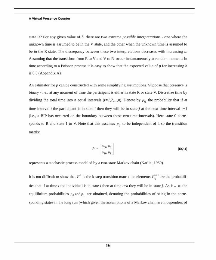
An estimator for p can be constructed with some simplifying assumptions. Suppose that presence is
binary - i.e., at any moment of time the participant is either in state R or state V. Discretize time by
dividing the total time into n equal intervals (t=1,2,...,n). Denote by the probability that if at
time interval t the participant is in state i then they will be in state j at the next time interval t+1
(i.e., a BIP has occurred on the boundary between these two time intervals). Here state 0 corre-
sponds to R and state 1 to V. Note that this assumes to be independent of t, so the transition
matrix:
(EQ 1)
represents a stochastic process modeled by a two-state Markov chain (Karlin, 1969).
It is not difficult to show that is the k-step transition matrix, its elements are the probabili-
ties that if at time t the individual is in state i then at time t+k they will be in state j. As the
equilibrium probabilities are obtained, denoting the probabilities of being in the corre-
sponding states in the long run (which given the assumptions of a Markov chain are independent of
pij
pij
Pp00 p01
p10 p11
=
Pk
Pijk( )
k ∞→
p0 and p1
16
A Virtual Presence Counter
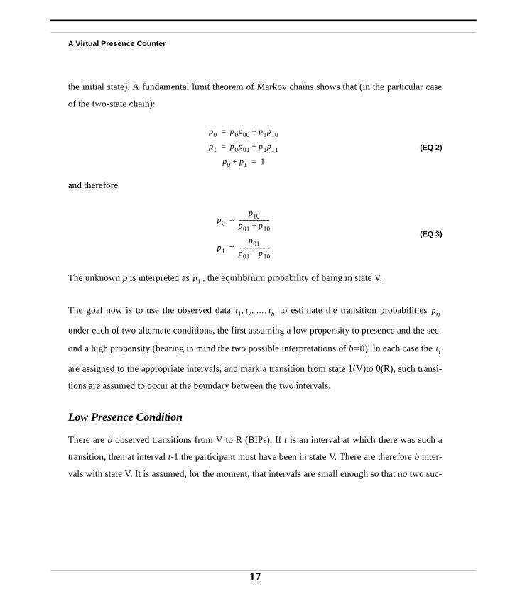
the initial state). A fundamental limit theorem of Markov chains shows that (in the particular case
of the two-state chain):
(EQ 2)
and therefore
(EQ 3)
The unknown p is interpreted as , the equilibrium probability of being in state V.
The goal now is to use the observed data to estimate the transition probabilities
under each of two alternate conditions, the first assuming a low propensity to presence and the sec-
ond a high propensity (bearing in mind the two possible interpretations of b=0). In each case the
are assigned to the appropriate intervals, and mark a transition from state 1(V)to 0(R), such transi-
tions are assumed to occur at the boundary between the two intervals.
Low Presence Condition
There are b observed transitions from V to R (BIPs). If t is an interval at which there was such a
transition, then at interval t-1 the participant must have been in state V. There are therefore b inter-
vals with state V. It is assumed, for the moment, that intervals are small enough so that no two suc-
p0 p0p00 p1p10+=
p1 p0p01 p1p11+=
p0 p1+ 1=
p0
p10
p01 p10+----------------------=
p1
p01
p01 p10+----------------------=
p1
t1 t2 … tb, , , pij
ti
17
A Virtual Presence Counter
cessive states reported a BIP, and that the first and last intervals did not report a BIP. In the low
presence condition, it is assumed that all intervals in which the state is unknown are in state 0.
is the proportion of times that an interval in state 0 is followed by an interval also in state 0.
There are intervals in state 0 that are followed by another interval (interval n has no suc-
cessor). All but b of them are followed by intervals in state 0. Therefore
(EQ 4)
is the proportion of times that an interval in state 1 is followed by an interval in state 0. Since
this always occurs,
(EQ 5)
From these the equilibrium probabilities are:
(EQ 6)
High Presence Condition
In this case the assumption is that all intervals in which the state is unknown are in the state V(1). A
similar analysis to that above yields:
p00
n 1– b–
p00n 1– 2b–n 1– b–------------------------=
p01b
n 1– b–---------------------=
where 2b n 1–≤
p10
p10 1 and p11 0= =
p0n 1– b–
n 1–---------------------=
p1b
n 1–------------=
where 2b n 1–≤
18
A Virtual Presence Counter
about
max-
o
of the
(EQ 7)
Let be the equilibrium probability of being in state V with b BIPs observed and with c corre-
sponding to the Low Presence (L) condition, or the High Presence (H) condition, then:
(EQ 8)
Figure 2, “Relationship between number of BIPs (b) and overall presence (p),” on page 49
here.
The relationship is illustrated in Figure 2, showing that when the number of BIPs achieves its
imum .
Figure 2 highlights a problem: in practice only b is observed, and for any level of b there are two
extreme values of p. Knowing only b gives insufficient information to estimate p. To choose
between and , therefore, a discriminator is required - some additional information t
select one of the two alternatives. The simplest way to achieve this is a question at the end
p0b
n 1–------------=
p1n 1– b–
n 1–---------------------=
where 2b n 1–≤
pc b( )
pL b( ) bn 1–------------=
pH b( ) n 1– b–n 1–
---------------------=
where 2b n 1–≤
n 1–( ) 2 p,⁄ 0.5=
pL b( ) pH b( )
19
A Virtual Presence Counter
proba-
eport a
le to
session, asking the participant to classify their overall experience with respect to their sense of pres-
ence. The answer to this together with the value of b would then allow an estimate of p.
It should be recalled that this analysis gives, for any condition, two extreme interpretations. For
example, in the low presence condition, the analysis implies:
(EQ 9)
In the absence of prior information it would be normal to use an estimate half-way between these
two bounds. Such estimates would be linear transforms of and , and therefore would
have no effect on relationships with other variables discovered in statistical analysis. Therefore this
paper continues to use and , which should properly be referenced as ‘extremal
bilities’, although the qualifier ‘extremal’ is usually dropped.
Special Cases
For any choice of time interval, there can always be a situation where successive intervals r
BIP, or where there is a BIP in the first interval or in the last interval. It is important to be ab
bn 1–------------ p
12---<≤
pL b( ) pH b( )
pL b( ) pH b( )
20
A Virtual Presence Counter
cater for these special cases, in order to avoid the problem of having to choose very large values of
n, thus forcing the probabilities to the extremes.
The analysis can be easily adjusted to take account of this. One additional assumption is made,
which is that if there are successive BIPs then the amount of time in the V state in between them is
negligible.
Suppose that k out of the b BIPs are followed by a BIP in the next interval. Then the transition
matrix probabilities are as follows:
(EQ 10)
with
(EQ 11)
(EQ 12)
with
(EQ 13)
A further refinement allows for a BIP in the first or last intervals. Let if there is a BIP in the
first interval, and 0 otherwise, and similarly if there is a BIP in the last interval, and 0 other-
P low presence–( )n 1– 2 b k–( )–
n 1– b– k+-------------------------------------
b k–n 1– b– k+------------------------------
1 0
=
pL b( ) b k–n 1–------------=
P high presence–( )
kb---
b k–b
-----------
b k–n 1– b–---------------------
n 1– 2b– k+n 1– b–
---------------------------------
=
pH b( ) n 1– b–n 1–
---------------------=
s1 1=
sn 1=
21
A Virtual Presence Counter
es for
corre-
cted
on the
graph
ique is
ation
othe-
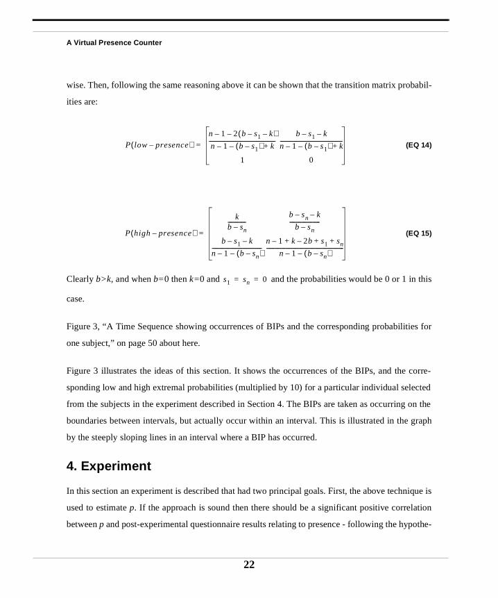
wise. Then, following the same reasoning above it can be shown that the transition matrix probabil-
ities are:
(EQ 14)
(EQ 15)
Clearly b>k, and when b=0 then k=0 and and the probabilities would be 0 or 1 in this
case.
Figure 3, “A Time Sequence showing occurrences of BIPs and the corresponding probabiliti
one subject,” on page 50 about here.
Figure 3 illustrates the ideas of this section. It shows the occurrences of the BIPs, and the
sponding low and high extremal probabilities (multiplied by 10) for a particular individual sele
from the subjects in the experiment described in Section 4. The BIPs are taken as occurring
boundaries between intervals, but actually occur within an interval. This is illustrated in the
by the steeply sloping lines in an interval where a BIP has occurred.
4. Experiment
In this section an experiment is described that had two principal goals. First, the above techn
used to estimate p. If the approach is sound then there should be a significant positive correl
between p and post-experimental questionnaire results relating to presence - following the hyp
P low presence–( )n 1– 2 b s1 k––( )–
n 1– b s1–( )– k+------------------------------------------------
b s1 k––
n 1– b s1–( )– k+---------------------------------------------
1 0
=
P high presence–( )
kb sn–-------------
b sn k––
b sn–----------------------
b s1 k––
n 1– b sn–( )–------------------------------------
n 1– k 2b– s1 sn+ + +
n 1– b sn–( )–--------------------------------------------------------
=
s1 sn 0= =
22
A Virtual Presence Counter
sis that these questions are answered on the basis of the balance of time that a participant spends in
the V compared to the R state. Second, previous results (for example, Slater, Steed, McCarthy &
Maringelli, 1998; Usoh, Arthur, Whitton, Bastos, Steed, Slater & Brooks, 1999) suggest a positive
relationship between the degree of body movement of a participant and their reported presence. The
experiment also examines this idea in a different context to those previous studies.
The experimental scenario involved the participants observing a sequence of moves on a Tri-
dimensional chess board (as introduced by the Star Trek TV series). This was chosen because it is a
quite large and complex three-dimensional object, and fitted well with the requirement to induce
significant body movement in participants who were required to reach out and touch the chess
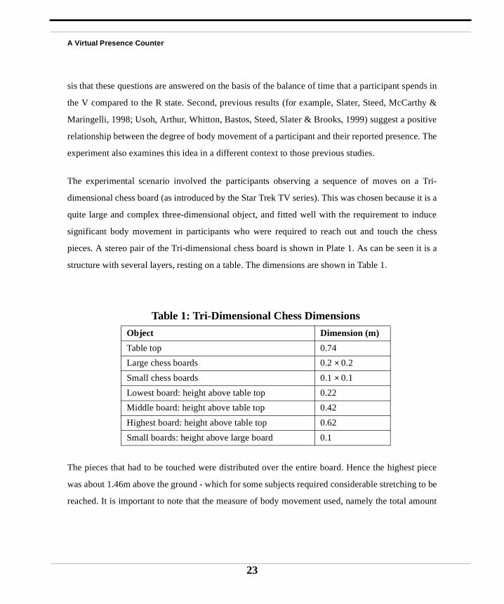
pieces. A stereo pair of the Tri-dimensional chess board is shown in Plate 1. As can be seen it is a
structure with several layers, resting on a table. The dimensions are shown in Table 1.
The pieces that had to be touched were distributed over the entire board. Hence the highest piece
was about 1.46m above the ground - which for some subjects required considerable stretching to be
reached. It is important to note that the measure of body movement used, namely the total amount
Table 1: Tri-Dimensional Chess Dimensions
Object Dimension (m)
Table top 0.74
Large chess boards 0.2 × 0.2
Small chess boards 0.1 × 0.1
Lowest board: height above table top 0.22
Middle board: height above table top 0.42
Highest board: height above table top 0.62
Small boards: height above large board 0.1
23
A Virtual Presence Counter
s were
r sub-
ere 18
under-
iscella-
lf.
fter
plants
lates 2
hess
t, and
that
se) and
on the
ton
l red
hould
of hand movement, is of course, a measure of whole body movement - since it would encompass
such reaching and stretching.
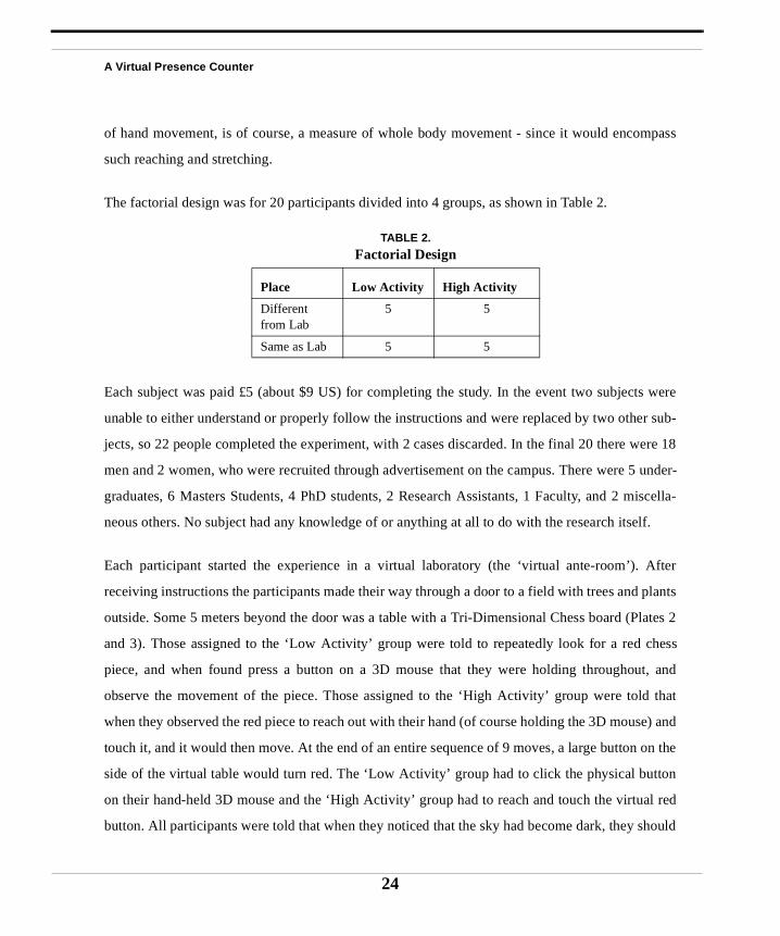
The factorial design was for 20 participants divided into 4 groups, as shown in Table 2.
Each subject was paid £5 (about $9 US) for completing the study. In the event two subject
unable to either understand or properly follow the instructions and were replaced by two othe
jects, so 22 people completed the experiment, with 2 cases discarded. In the final 20 there w
men and 2 women, who were recruited through advertisement on the campus. There were 5
graduates, 6 Masters Students, 4 PhD students, 2 Research Assistants, 1 Faculty, and 2 m
neous others. No subject had any knowledge of or anything at all to do with the research itse
Each participant started the experience in a virtual laboratory (the ‘virtual ante-room’). A
receiving instructions the participants made their way through a door to a field with trees and
outside. Some 5 meters beyond the door was a table with a Tri-Dimensional Chess board (P
and 3). Those assigned to the ‘Low Activity’ group were told to repeatedly look for a red c
piece, and when found press a button on a 3D mouse that they were holding throughou
observe the movement of the piece. Those assigned to the ‘High Activity’ group were told
when they observed the red piece to reach out with their hand (of course holding the 3D mou
touch it, and it would then move. At the end of an entire sequence of 9 moves, a large button
side of the virtual table would turn red. The ‘Low Activity’ group had to click the physical but
on their hand-held 3D mouse and the ‘High Activity’ group had to reach and touch the virtua
button. All participants were told that when they noticed that the sky had become dark, they s
TABLE 2.
Factorial Design
Place Low Activity High Activity
Different from Lab
5 5
Same as Lab 5 5
24
A Virtual Presence Counter
f and
. After
d then
chess
d cube
ce
return from the field to the starting room. The sky was darkened after three complete sequences of
moves, and the mean and standard deviation of the time spent in the field was 319±64s. All subjects
were told that they would be asked about the sequence of moves observed after the experience.
Prior to starting the experiment all subjects were asked to complete a short questionnaire that
obtained background information - gender, job status, and prior experience of virtual reality.
After completing the questionnaire, the subject was shown each of Figure 1b-d in turn. (Most sub-
jects had seen Figure 1b before, so that this was hardly used). They were asked to describe their ini-
tial interpretation of the figure. (For example, for Figure 1c, most saw the three thin triangles first
of all). Then they were asked to stare at the figure, and notice if any change occurred. If a change
did happen, they were asked to continue to observe the figure and clearly exclaim ‘Now!’ i
whenever it spontaneously reconfigured itself to look the same way as when they first saw it
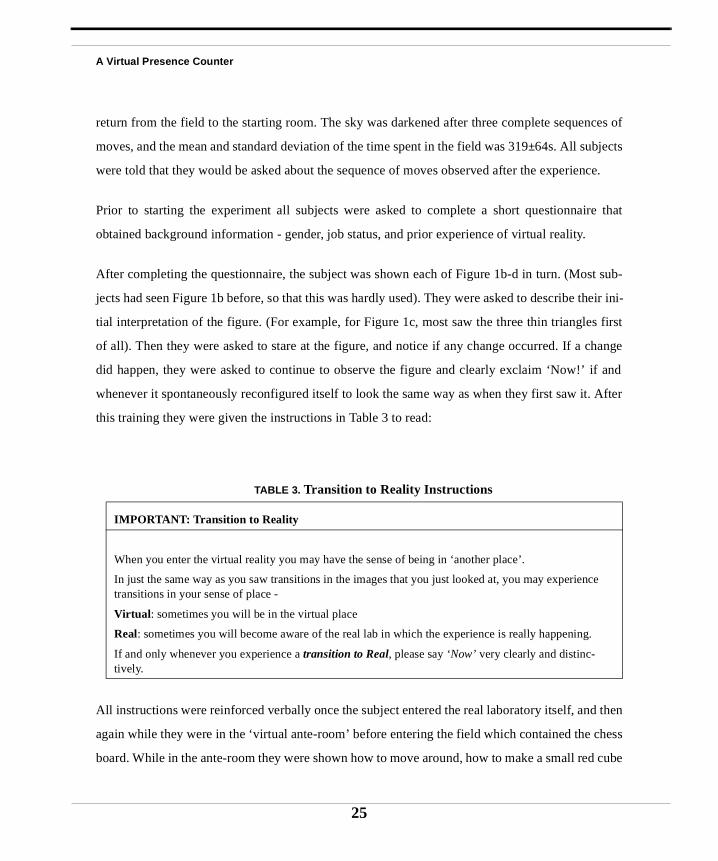
this training they were given the instructions in Table 3 to read:
All instructions were reinforced verbally once the subject entered the real laboratory itself, an
again while they were in the ‘virtual ante-room’ before entering the field which contained the
board. While in the ante-room they were shown how to move around, how to make a small re
TABLE 3. Transition to Reality Instructions
IMPORTANT: Transition to Reality
When you enter the virtual reality you may have the sense of being in ‘another place’.
In just the same way as you saw transitions in the images that you just looked at, you may experientransitions in your sense of place -
Virtual: sometimes you will be in the virtual place
Real: sometimes you will become aware of the real lab in which the experience is really happening.
If and only whenever you experience a transition to Real, please say ‘Now’ very clearly and distinc-tively.
25
A Virtual Presence Counter
er
re is
ngs or
room
events
finite
3.1.2.
ton 3D
in ste-
thumb
they
his was
for the
tions:
ran-
quired
on a table respond by either touching it (‘High Activity’ group) or by clicking with their forefing
on the 3D mouse (‘Low Activity’ group).
The virtual reality laboratory is in a small enclosed room within a large laboratory, in which the
continual noise (constant noise of workstations, and random noise of occasional phone ri
conversations). No attempt was made to reduce background noise or further isolate the VR
from the remainder of the laboratory: indeed there was interest as to whether the background
would trigger transitions from V to R.
The scenarios were implemented on a Silicon Graphics Onyx with twin 196 MHz R10000, In
Reality Graphics and 64M main memory. The software used was Division’s dVS and dVISE
The tracking system has two Polhemus Fastraks, one for the HMD and another for a 5 but
mouse. The helmet was a Virtual Research VR4 which has a resolution of 742×230 pixels for each
eye, 170,660 color elements and a field-of-view 67 degrees diagonal at 85% overlap.
The total scene consisted of 13298 polygons which ran at a frame rate of no less than 20 Hz
reo. The latency was approximately 120 ms.
Subjects moved through the environment in gaze direction at constant velocity by pressing a
button on the 3D mouse. They had a simple inverse kinematic virtual body (Plate 4). When
reached forward to touch a chess piece they would see their virtual arm and hand.
At the end of the session subjects were given a second questionnaire. The main purpose of t
to gather information on their sense of presence. There was an initial question that asked
reason why (if this was the case) they reported no or very few transitions, giving four op
rarely being in the virtual world, almost always being in the virtual world, forgetting to report t
sitions, other reasons. In retrospect this question was not particularly useful, since it only re
26
A Virtual Presence Counter
this.
t these
through
. These
ussed
e and
ts
ty” forence
an answer when subjects reported ‘no or very few transitions’ without giving a definition of
No subject reported forgetting the instruction to report transitions.
A second question was open ended, asking for the ‘causes of the transitions’ (whether or no
had been reported at the time). There were five questions relating to presence interspersed
the questionnaire, each rated on a 1 to 7 scale, where 1 indicated low and 7 high presence
questions followed the same model introduced in (Slater, Steed & Usoh, 1993) as briefly disc
in Section 2. The first question was a priori considered the most direct elicitation of presenc
used as the discriminator: a score of more than 4 on this resulted in the formula pH(b) being used,
otherwise pL(b).
1. Please rate your sense of being in the field, on the following scale from 1 to 7, where 7 represenyour normal experience of being in a place.I had a sense of “being there” in the field:1. Not at all ... 7. Very much.
2. To what extent were there times during the experience when the field became the “realiyou, and you almost forgot about the “real world” of the laboratory in which the whole experiwas really taking place?There were times during the experience when the virtual field became more real for me comparedto the “real world”...1. At no time ... 7. Almost all the time.
3. When you think back about your experience, do you think of the field more as images that yousaw, or more as somewhere that you visited? Please answer on the following 1 to 7 scale:The virtual field seems to me to be more like...1. images that I saw ...7. somewhere that I visited.
4. During the time of the experience, which was strongest on the whole, your sense of being in thefield, or of being in the real world of the laboratory?I had a stronger sense of being in...1. the real world of the laboratory ... 7. the virtual reality of the field of plants.
27
A Virtual Presence Counter
t of
n of the
s were
estions,
el 5 or
is was
re was a
number
5. During the time of the experience, did you often think to yourself that you were actually juststanding in an office wearing a helmet or did the field overwhelm you?During the experience I often thought that I was really standing in the lab wearing a helmet....1. most of the time I realised I was in the lab ... 7. never because the virtual field overwhelmed me.
Some data were automatically collected during the course of the experiment - in particular the
times at which the participant said ‘Now!’ and the total time in the virtual field. The amoun
hand and head movement was computed by the program running the simulation as a functio
head and hand tracking.
5. Results
5.1 General
The overall levels of reported ‘presence’ as ascertained from the questionnaire response
high. Figure 4 shows the median response for each for each of the five presence related qu
showing, for example, that on question 1 (the discriminator) half of the responses were at lev
more.
Figure 4, “Median Levels of reported presence,” on page 51 about here
The number of BIPs ranged between 0 and 14. The mean time between BIPs was 48±37s, the mini-
mum time interval was 5.5s and the maximum 141s. The time interval used for the analys
10s, this being approximately the largest compatible with the assumptions that 2b ≤ n-1. There
were two cases where there were some BIPs in sequence, and two other cases where the
BIP in the first or last interval.
The Questionnaire based presence, using all five presence questions, is plotted against the
of BIPS, in Figure 5.
Figure 5, “Number of BIPs by Questionnaire Presence,” on page 52 about here.
28
A Virtual Presence Counter
t of 4,
ding
ves
lar
the VE,
o them
ecord
ponse
each
resence
4
is
ave a
ce in
5.2 Relationship between p and Questionnaire Based Presence
The first question to consider is whether there is a relationship between the estimate of presence p,
and the presence questionnaire responses. The usual approach of the authors to combining the
results of the presence questions into one overall score (without resorting to averaging across ordi-
nal data) is to count the number of high scores (‘6’ or ‘7’), thus giving each subject a count ou
for the questions other than that used as the discriminator (questions 2 to 5 above).
Figure 6, “Scatter Plot of p Against Questionnaire Presence,” on page 53 about here.
Figure 6 shows the scatter plot of p against the questionnaire presence count (recall that thep’s are
‘extremal’). There is a clear positive relationship, though with an outlying point. Even inclu
this point there is a statistically significant correlation between p and the presence count (r2 = 0.32,
t = 2.920, t18 = 2.101 at 5% significance level). When this outlier is removed the result impro
substantially (r2 = 0.65, t = 5.588, t17 = 3.965 at 0.1%). Examining the responses of the particu
person represented by the outlier, he wrote that he was disturbed by the absence of sound in
knew that the experimenters were in the real lab alongside him, and that he wanted to talk t
because exploring an environment is often a “communal activity”. The experimenter’s notes r
that he did indeed continue to talk to them during the immersive experience. He gave a ‘3’ res
to the discriminator question (writing “SOUND!” next to his response), and scores of ‘7’ for
of the remaining four presence-related questions. The assignment of this person to the low p
condition on the basis of this particular discriminator is therefore dubious.
5.3 Relationship between p and Hand Activity
The next issue to consider is the relationship between p and the main independent factors. Table
shows the means and standard deviations of p for the activity groups, and the difference in means
not significant although contrary to expectation, the low activity group seems at first sight to h
higher ‘average presence’ than the high activity group. There is a highly significant differen
29
A Virtual Presence Counter
,
sig-
n of
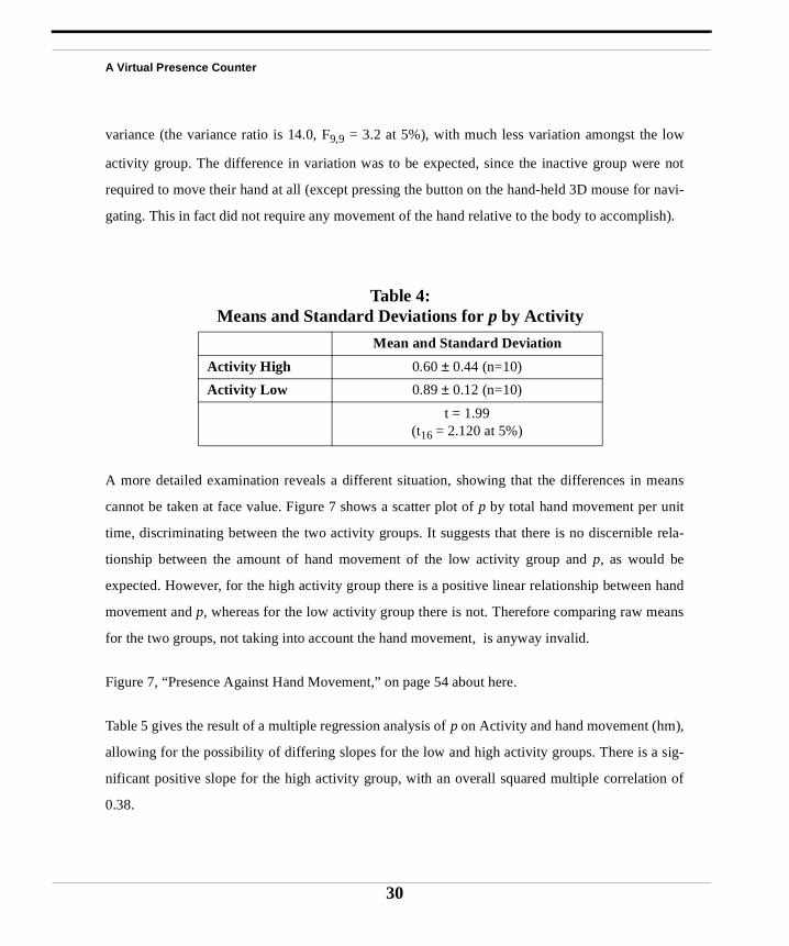
variance (the variance ratio is 14.0, F9,9 = 3.2 at 5%), with much less variation amongst the low
activity group. The difference in variation was to be expected, since the inactive group were not
required to move their hand at all (except pressing the button on the hand-held 3D mouse for navi-
gating. This in fact did not require any movement of the hand relative to the body to accomplish).
A more detailed examination reveals a different situation, showing that the differences in means
cannot be taken at face value. Figure 7 shows a scatter plot of p by total hand movement per unit
time, discriminating between the two activity groups. It suggests that there is no discernible rela-
tionship between the amount of hand movement of the low activity group and p, as would be
expected. However, for the high activity group there is a positive linear relationship between hand
movement and p, whereas for the low activity group there is not. Therefore comparing raw means
for the two groups, not taking into account the hand movement, is anyway invalid.
Figure 7, “Presence Against Hand Movement,” on page 54 about here.
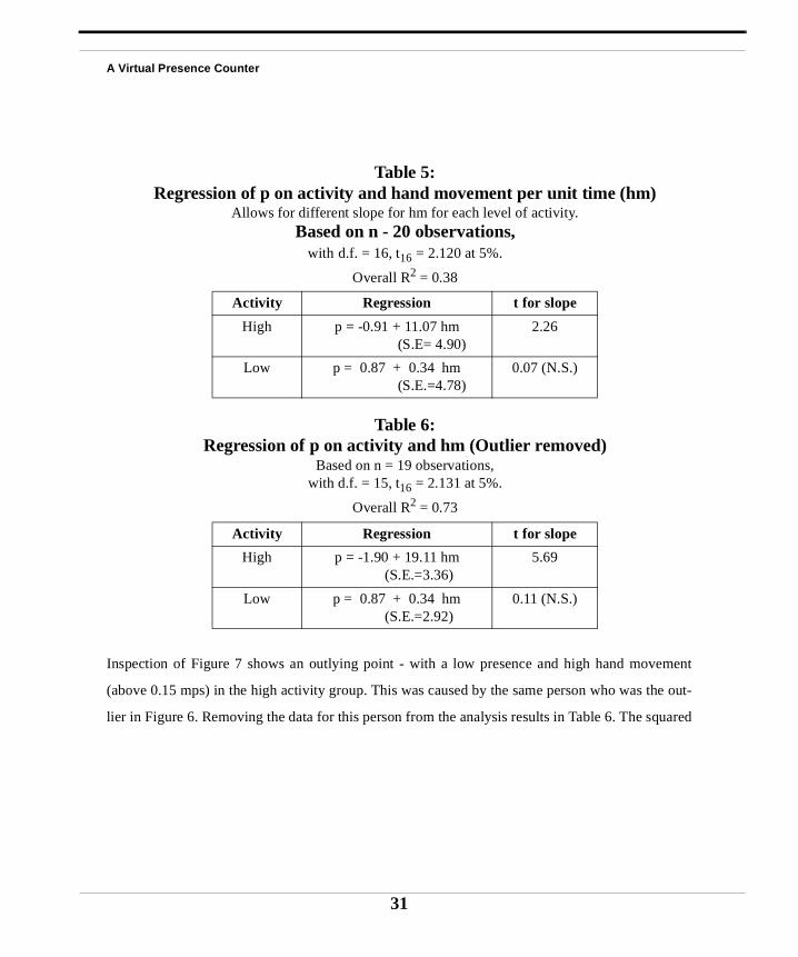
Table 5 gives the result of a multiple regression analysis of p on Activity and hand movement (hm)
allowing for the possibility of differing slopes for the low and high activity groups. There is a
nificant positive slope for the high activity group, with an overall squared multiple correlatio
0.38.
Table 4: Means and Standard Deviations for p by Activity
Mean and Standard Deviation
Activity High 0.60 ± 0.44 (n=10)
Activity Low 0.89 ± 0.12 (n=10)
t = 1.99(t16 = 2.120 at 5%)
30
A Virtual Presence Counter
Inspection of Figure 7 shows an outlying point - with a low presence and high hand movement
(above 0.15 mps) in the high activity group. This was caused by the same person who was the out-
lier in Figure 6. Removing the data for this person from the analysis results in Table 6. The squared
Table 5: Regression of p on activity and hand movement per unit time (hm)
Allows for different slope for hm for each level of activity.Based on n - 20 observations,
with d.f. = 16, t16 = 2.120 at 5%.
Overall R2 = 0.38
Activity Regression t for slope
High p = -0.91 + 11.07 hm (S.E= 4.90)
2.26
Low p = 0.87 + 0.34 hm (S.E.=4.78)
0.07 (N.S.)
Table 6: Regression of p on activity and hm (Outlier removed)
Based on n = 19 observations,with d.f. = 15, t16 = 2.131 at 5%.
Overall R2 = 0.73
Activity Regression t for slope
High p = -1.90 + 19.11 hm (S.E.=3.36)
5.69
Low p = 0.87 + 0.34 hm (S.E.=2.92)
0.11 (N.S.)
31
A Virtual Presence Counter
the
.
being
vir-
multiple correlation increases to 0.73, and the slope for the high activity group is well into the
highly significant range.
Explanations for BIPs
A question asked the participants to give the reasons for their transitions to the real:
If you did make transitions from virtual to real, whether or not you reported these at the time, what
do you remember as the causes of the transitions? (For example, hearing an unexpected noise from
the real lab might cause such a transition).
The reasons given can be classified into two main (most often reported) types:
External: Sensory information from the real world intruded into or contradicted the virtual world,
either in the form of noises or people talking, or else the touch or feel of interactions with real solid
objects (such as the virtual reality equipment itself).
Internal: This is where something ‘wrong’ with the virtual world itself is noticed: for example,
laws of physics not being obeyed, objects looking unreal, the absence of sounds, display lag
There were a number of subsidiary reasons:
Experiment: Some aspect of the experimental set-up itself, or the instructions intruded.
Personal: Some personal feeling intruding, such as embarrassment or consciousness of
observed from the outside.
Attention: A loss of attention to what is happening in the virtual world, or some aspect of the
tual world that results in a loss of presence.
Spontaneous: A BIP for no (conscious) apparent reason.
32
A Virtual Presence Counter
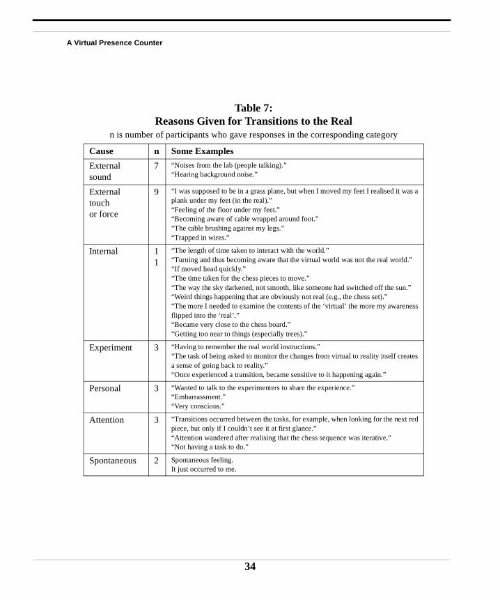
Table 7 gives the number of participants who responded in each of these categories, and some
examples of each.
33
A Virtual Presence Counter
Table 7: Reasons Given for Transitions to the Real
n is number of participants who gave responses in the corresponding category
Cause n Some Examples
Externalsound
7 “Noises from the lab (people talking).”“Hearing background noise.”
Externaltouch or force
9 “I was supposed to be in a grass plane, but when I moved my feet I realised it was aplank under my feet (in the real).”“Feeling of the floor under my feet.”“Becoming aware of cable wrapped around foot.”“The cable brushing against my legs.”“Trapped in wires.”
Internal 11
“The length of time taken to interact with the world.” “Turning and thus becoming aware that the virtual world was not the real world.”“If moved head quickly.”“The time taken for the chess pieces to move.” “The way the sky darkened, not smooth, like someone had switched off the sun.”“Weird things happening that are obviously not real (e.g., the chess set).”“The more I needed to examine the contents of the ‘virtual’ the more my awarenessflipped into the ‘real’.” “Became very close to the chess board.” “Getting too near to things (especially trees).”
Experiment 3 “Having to remember the real world instructions.”“The task of being asked to monitor the changes from virtual to reality itself createsa sense of going back to reality.”“Once experienced a transition, became sensitive to it happening again.”
Personal 3 “Wanted to talk to the experimenters to share the experience.” “Embarrassment.”“Very conscious.”
Attention 3 “Transitions occurred between the tasks, for example, when looking for the next redpiece, but only if I couldn’t see it at first glance.” “Attention wandered after realising that the chess sequence was iterative.”“Not having a task to do.”
Spontaneous 2 Spontaneous feeling.It just occurred to me.
34
A Virtual Presence Counter
s each
f
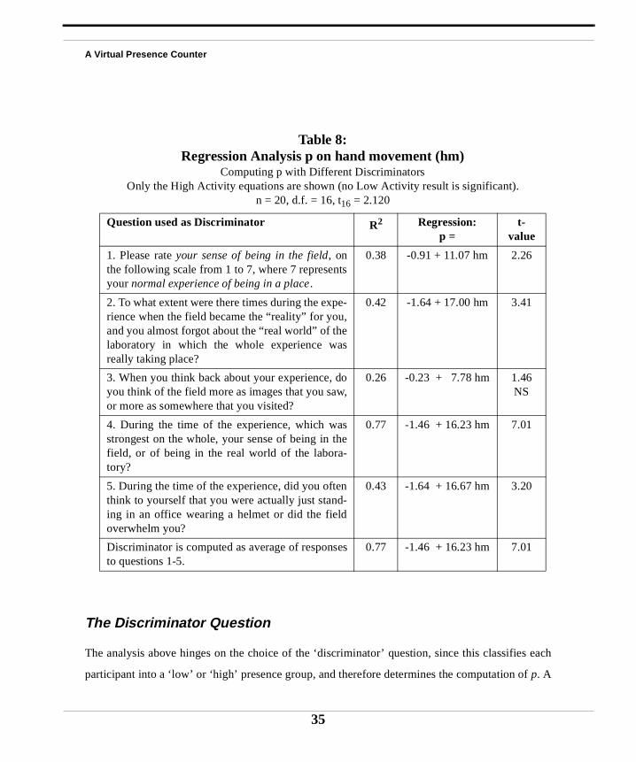
The Discriminator Question
The analysis above hinges on the choice of the ‘discriminator’ question, since this classifie
participant into a ‘low’ or ‘high’ presence group, and therefore determines the computation op. A
Table 8: Regression Analysis p on hand movement (hm)
Computing p with Different DiscriminatorsOnly the High Activity equations are shown (no Low Activity result is significant).
n = 20, d.f. = 16, t16 = 2.120
Question used as Discriminator R2 Regression: p =
t-value
1. Please rate your sense of being in the field, onthe following scale from 1 to 7, where 7 representsyour normal experience of being in a place.
0.38 -0.91 + 11.07 hm 2.26
2. To what extent were there times during the expe-rience when the field became the “reality” for you,and you almost forgot about the “real world” of thelaboratory in which the whole experience wasreally taking place?
0.42 -1.64 + 17.00 hm 3.41
3. When you think back about your experience, doyou think of the field more as images that you saw,or more as somewhere that you visited?
0.26 -0.23 + 7.78 hm 1.46NS
4. During the time of the experience, which wasstrongest on the whole, your sense of being in thefield, or of being in the real world of the labora-tory?
0.77 -1.46 + 16.23 hm 7.01
5. During the time of the experience, did you oftenthink to yourself that you were actually just stand-ing in an office wearing a helmet or did the fieldoverwhelm you?
0.43 -1.64 + 16.67 hm 3.20
Discriminator is computed as average of responsesto questions 1-5.
0.77 -1.46 + 16.23 hm 7.01
35
A Virtual Presence Counter
to
ny of
stion,
ce ques-
ctly the
cesses
f the
r of the
an indi-
odel
tead.
l is sta-
ion is
different discriminator question could lead to quite different results. However, the results for this
experiment are robust with respect to choice of discriminator question.
The analysis was repeated for each of the remaining four presence-related questions, and also for
the average of all of the five questions (Table 8). (Of course, the ‘outlying point’ corresponding
someone who had written ‘3’ for question 1, but ‘7’ for each of the others, does not occur for a
the choices of discriminator other than question 1). For every choice of discriminator que
except for question 3, the results are the same. When the mean response of all of the presen
tions is used as discriminator, again the results are the same. (Note that question 4 has exa
same impact as a discriminator as the average).
6. Discussion
The method presented in this paper relies on a number of assumptions.
1. Presence in the ‘real’ and ‘virtual’ is treated as a binary state.
The authors would not seek to defend this as a statement about the psychological pro
involved. It is used here in the spirit of a simplifying assumption, to allow the construction o
stochastic model. However, arguments were presented at the conclusion of Section 2 in favo
notion that presence may be considered as a selection of one environment relative to which
vidual acts at a given moment.
2. The stochastic model assumes discrete time.
Again this is a simplifying assumption often employed in the initial stages of constructing a m
of complex phenomena. It may be possible to employ a continuous time stochastic model ins
3. The transitions can be modeled as a Markov chain.
This assumes that the transition probabilities are one-step - that what happens in any interva
tistically independent of all other intervals except for the last. The veracity of this assumpt
36
A Virtual Presence Counter
unknown, and again should be viewed as a simplification for the purpose of the construction of an
initial model.
4. The requirement to report BIPs does not in itself influence the participants to report BIPs.
There is experimental evidence to support the argument that the requirement to report BIPs
increases the chance of BIPs occurring. Girgus, Rock & Egatz (1977) found that giving subjects a
knowledge of the reversibility of ambiguous figures substantially increased the chance of these
being reported. About half the subjects who were not told about the reversibility of figures never
reported a transition, whereas all of the subjects who were told about the reversibility always
reported transitions. This raises the possibility that more BIPs were reported than would otherwise
have naturally occurred.
This is a difficult issue, since it could also be argued that the requirement to report BIPs sets up a
dual task for the participants - to do their actual task in the VE and to pay attention to their state in
order to be able to report the BIPs. A counter argument to this is that it the requirement to report a
BIP is likely to only enter consciousness at the time immediately after a BIP has occurred (as dis-
cussed earlier).
A preferable response to these problems is to agree that the method for reporting BIPs, relying on a
verbal response is certainly not an ideal way to obtain this information. It is an interesting and chal-
lenging research topic to try to find physiological correlates to BIPs that can be measured unobtru-
sively.
5. The discriminator question can discriminate between the low and high propensity cases.
37
A Virtual Presence Counter
d been
esence,
mea-
owever,
as the
vement
sts
on the
but the
vement,
part of
ch the
they all
cts took
Use of a discriminator question does indeed result in an uncomfortable reliance on questionnaire
data. An alternative, behaviorally based discriminator, would be preferable.
7. Conclusions
Notwithstanding the critique above, a new method for measuring presence in virtual environments
has been introduced, where the major component of the measure depends on data collected during
the course of the VE experience itself. It is based on the number of transitions between a state of
being in the VE, to the state of being in the real world. Using the simplifying assumption that
changes in state between presence and non-presence form a time independent Markov chain, an
equilibrium probability of presence can be estimated. This requires only one additional post-exper-
imental discriminator question concerning each participant’s assessment of whether they ha
in the presence state for more or for less than half the time.
This new technique was tried in an experiment to assess the impact of body movement on pr
and was found to be positively and significantly correlated with the usual questionnaire based
sure. It is encouraging that the questionnaire score and the new measure were correlated. H
further studies are necessary for validation.
Another issue for the experiment apart from the methodology for presence measurement, w
relationship between presence and hand movement. (In this experiment head and hand mo
were significantly correlated, r2 = 0.54, t = 4.6, t18 = 2.101 at 5%). The evidence strongly sugge
a positive association between presence and hand movement, in line with previous evidence
relationship between presence and body movement. The direction of causality is unknown,
authors suspect that there is a two way relationship: high presence leads to greater body mo
and greater body movement reinforces high presence. There is some evidence for the first
this statement. Since subjects in the high activity group were all required to reach out and tou
chess pieces, why is there such high variation in their measured hand movements - since
had to reach the same distances? The variation can be explained by the fact that some subje
38
A Virtual Presence Counter
the most direct routes to the chess pieces, ignoring collisions with the board and other pieces,
whereas others acted more as they would have in real life - avoiding collisions with other objects.
Hence, it could be argued that presence in the VE caused them to act this way, thus leading to
greater body movement.
The relationship between presence and body movement follows from the notion that one of the
most important determinants for presence is the requirement for a match between proprioception
and sensory data. This is consequential for the design of interaction paradigms - where semantically
appropriate body movement, exploiting proprioception, is preferred, for example, to the importa-
tion of techniques from 2D interfaces. This relationship between presence and proprioception in the
design of interaction paradigms has been exploited in several studies (Slater, Usoh & Steed, 1995;
Mine, Brooks & Sequin, 1997; Grant & Magree, 1998; Usoh, Arthur, Whitton, Bastos, Steed, Slater
& Brooks, 1999).
There are some recommendations for future use of the new measure. First, the discriminator ques-
tion should ask for the information that is required in a very direct manner. (Question 4 would have
been preferable to question 1). As soon as the VE experience has terminated, the participant should
be asked to estimate the overall proportion of time spent in the presence state, crucially whether
above or below 50 per cent. The exact wording of this discriminator question, or indeed as noted in
Section 6, whether there is some better way to obtain this information should be given more
thought.
Second, a standard time interval should be agreed, so that results can be easily compared between
different applications and systems. In this experiment the time interval was chosen to be the great-
est compatible with the requirement that 2b ≤ n-1 (n is the number of intervals). The interval used
was 10 seconds. The choice of large values of n grants undue weight to the statistical significance
39
A Virtual Presence Counter
being
r body
nsional
k V.
ofes-
com-
of the count data, and pushes the probability estimates to more extreme values (though does not
alter the relationship between them).
The results are nevertheless robust with respect to the range of time intervals. An analysis with
intervals ranging from 1 second through to the maximum compatible with the crucial requirement
of 2b ≤ n-1 always gives the same results. A preferable solution would be to construct a model that
does not require the use of discrete time intervals.
Finally, to return to the issue of body movement. In the Tri-dimensional chess experiment, it is
clear that many of the (active) subjects are learning about the chess board with their whole bodies.
As stated earlier, to call the movements ‘hand movements’ is an understatement of what is
measured. It is not surprising that amongst the active group those who exhibited greate
movement also tended to have a greater sense of ‘being’ in the same space as the tri-dime
chess board.
Acknowledgments
This work is funded by the European ACTS COVEN Project. The authors would like to than
Linakis for the model of the Tri-dimensional chess board. The authors would like to thank Pr
sor Frederick Brooks Jnr, University of North Carolina, for his encouragement and helpful
ments.
40
A Virtual Presence Counter
n the, 5(2),
eoper-
Virtual
afened
References
Barfield & Weghorst, 1993Barfield & Weghorst (1993)Barfield, W. and Weghorst, S. (1993) The sense of presence within virtual environments: A concep-tual framework. In G. Salvendy and M. Smith (Eds.), Human computer interaction: Software andhardware interfaces (pp.699-704). Amsterdam: Elsevier.
Bystrom, Barfield & Hendrix, 1999Bystrom, Barfield & Hendrix (1999)Bystrom, K-E., Barfield, W. and Hendrix, C. (1999) A Conceptual Model of the Sense of Presencein Virtual Environments, Presence: Teleoperators and Virtual Environments, 8(2), 241-244.
Draper, Kaber & Usher, 1998Draper, Kabur & Usher (1998)Draper, J.V., Kaber, D.B. and Usher, J.M. (1998) Telepresence, Human Factors 40(3), 354-375.
Ellis, 1996Ellis (1996)Ellis, S.R. (1996) Presence of Mind: A Reaction to Thomas Sheridan’s “Further Musings oPsychophysics of Presence”, Presence: Teleoperators and Virtual Environments, MIT Press247-259.
Flach & Holden, 1998Flach, J.M. and Holden, J.G. (1998) The Reality of Experience: Gibson’s Way, Presence: Telators and Virtual Environments, 7(1), 90-95.
Freeman, Avons, Pearson & IJsselstijn, 1999Freeman, Avons, Pearson & IJsselstijn (1999)Freeman, J., Avons, S.E., Pearson, D.E. and IJsselstijn, W.A. (1999) Effects of Sensory Informationand Prior Experience on Direct Subjective Ratings of Presence, Presence: Teleoperators andEnvironments, 8(1), 1-13.
Gilkey & Weisenberger, 1995Gilkey & Weisenberger (1995)Gilkey, R.H. and Weisenberger, J.M. (1995) The Sense of Presence for the Suddenly DeAdult, Presence: Teleoperators and Virtual Environments, 4(4), 357-363.
Girgus, Rock & Egatz, 1977Girgus, Rock & Egatz (1977)
41
A Virtual Presence Counter
Girgus, J.J., Rock, I., Egatz, R. (1977) The Effect of Knowledge of Reversibility on the Reversibil-ity of Ambiguous Figures, Perception and Psychophysics, 22(6), 550-556.
Grant & Magree, 1998Grant, S.C. & Magee, L.E. (1998) Contributions of Proprioception to Navigation in Virtual Envi-ronments, Human Factors, 40(3), 489-497.
Hendrix & Barfield, 1996aHendrix & Barfield (1996a)Hendrix, C. and Barfield, W. (1996a) Presence within Virtual Environments as a Function of VisualDisplay Parameters, Presence: Teleoperators and Virtual Environments, MIT Press, 5(3), 274-289.
Hendrix & Barfield, 1996bHendrix & Barfield (1996b)Hendrix, C. and Barfield, W. (1996b) The Sense of Presence within Auditory Environments, Pres-ence: Teleoperators and Virtual Environments, MIT Press, 5(3), 290-301.
Held & Durlach, 1992Held & Durlach (1992)Held, R.M. and N.I. Durlach (1992) Telepresence, Presence: Teleoperators and Virtual Environ-ments, 1, winter 1992, MIT Press, 109-112.
Karlin, 1969Karlin, S. (1969) A First Course in Stochastic Processes, Academic Press.
Kohler, 1959Kohler, W. (1959) Gestalt psychology: An introduction to new concepts in modernpsychology. NY: Liverright, 1947; NY:NAL, 1959.
McGreevy, 1993McGreevy (1993)McGreevy, M.W. (1993) The Presence of Field Geologists in a Mars-Like Terrain, Presence: Tele-operators and Virtual Environments, 1(4) fall 1993, MIT Press, 375-403.
Mine, Brooks & Sequin, 1997Mine, M.R., Brooks, F.P, Jr., Sequin, C. (1997) Moving Objects in Space: Exploiting Propriocep-tion in Virtual-Environment Interaction, Computer Graphics (SIGGRAPH) Proceedings, 19-26.
Pausch, Proffit & Williams, 1997Pausch, Proffit & Williams (1997)Pausch, R., Proffit, D., Williams, G. (1997) Quantifying Immersion in Virtual Reality, Computer
42
A Virtual Presence Counter
Graphics (SIGGRAPH) Proceedings, 13-18.
Perls, Hefferline & Goodman, 1969Perls, F.S., Hefferline, R.F. and Goodman, P. (1969) Gestalt therapy; excitement and growth in thehuman personality, New York, Julian Press.
Prothero, Parker, Furness &Wells, 1995Prothero, Parker, Furness &Wells (1995)Prothero, J., Parker, D., Furness, T., & Wells, M. (1995). Towards a Robust, Quantitative Measureof Presence. In Proceedings of the Conference on Experimental Analysis and Measurement of Situ-ational Awareness, Datona Beach, FL, (pp. 359-366). Daytona Beach, FL: Embry-Riddle Aeronau-tical University Press.
Schloerb, 1995Schloerb (1995)Schloerb, D. (1995) A Quantitative Measure of Telepresence, Presence: Teleoperators and VirtualEnvironments, 4(1), 64-80.
Sheridan, 1992Sheridan (1992)Sheridan, T.B. (1992) Musings on Telepresence and Virtual Presence, Telepresence, Presence:Teleoperators and Virtual Environments, 1, winter 1992, MIT Press, 120-126.
Sheridan, 1996Sheridan, T.B. (1996) Further Musings on the Psychophysics of Presence, Presence: Teleoperatorsand Virtual Environments, MIT Press, 5(2), 241-246.
Slater, 1999Slater, M. (1999) Measuring Presence: A Response to the Witmer and Singer Presence Question-naire, Presence: Teleoperators and Virtual Environments, MIT Press, 8(5), in press.
Slater, Steed & Usoh, 1993Slater, Steed & Usoh (1993)Slater, M. Steed, A. and Usoh, M. (1993) The Virtual Treadmill: A Naturalistic Method for Naviga-tion in Immersive Virtual Environments, First Eurographics Workshop on Virtual Environments,Polytechnical University of Catalonia, ed. Martin Goebel, September 7, 1993, 71-83.
Slater, Usoh & Steed, 1994Slater, Usoh & Steed (1994)Slater, M., Usoh, M. and Steed, A. (1994) Depth of Presence in Virtual Environments, Presence:Teleoperators and Virtual Environments, 3.2 MIT Press, 1994, 130-144.
43
A Virtual Presence Counter
Slater, Usoh & Chrysanthou, 1995Slater, Usoh & Chrysanthou (1995)Slater, M., M. Usoh, Y. Chrysanthou (1995) The Influence of Dynamic Shadows on Presence inImmersive Virtual Environments, Second Eurographics Workshop on Virtual Reality, M. Goebel,ed., Monte Carlo, Jan., 1995.
Slater, Usoh & Steed, 1995Slater, M. Usoh, M., Steed, A. (1995) Taking Steps: The Influence of a Walking Metaphor on Pres-ence in Virtual Reality, ACM Transactions on Computer-Human Interaction (TOCHI) 2(3) Septem-ber, 201-219.
Slater & Wilbur, 1997Slater & Wilbur (1997)Slater, M., Wilbur S. (1997) A Framework for Immersive Virtual Environments (FIVE): Specula-tions on the Role of Presence in Virtual Environments, Presence: Teleoperators and Virtual Envi-ronments, 6(6) 603-616, MIT Press.
Slater, Steed, McCarthy & Maringelli, 1998Slater, Steed, McCarthy & Maringelli (1998)Slater, M., Steed, A., McCarthy, J., Maringelli, F. (1998) The Influence of Body Movement on Sub-jective Presence in Virtual Environments, Human Factors, 40(3), 469-477.
Snow & Williges, 1998Snow & Williges (1998)Snow, M.P. and Williges, R.C. (1998) Empirical Models Based on Free-Modulus Magnitude Esti-mation of Perceived Presence in Virtual Environments, Human Factors 40(3), 386-402.
Usoh, Arthur, Whitton, Bastos, Steed, Slater & Brooks, 1999Usoh, Arthur, Whitton, Bastos, Steed, Slater & Brooks (1999)Usoh M, Arthur K, Whitton M, Bastos R, Steed A, Slater M, Brooks F (1999) Walking > Walking-in-Place > Flying, in Virtual Envirionments, accepted for publication, Computer Graphics (SIG-GRAPH) 1999.
Welch, 1997Welch (1997)Welch, R.B. (1997) The Presence of Aftereffects, Advances in Human Factors/Ergonomics, 21A,Design of Computing Systems: Cognitive Considerations, (Eds). G. Salvendy, M.J. Smith, R.J.Koubek, 273-276, Elsevier: Amsterdam.
Welch, Blackman, Liu, Mellers & Stark, 1996Welch, Blackman, Liu, Mellers & Stark (1996)
44
A Virtual Presence Counter
Welch, R.B., Blackman, T.T., Liu, A., Mellers, B.A., Stark, L.W. (1996) The Effects of PictorialRealism, Delay of Visual Feedback, and Observer Interactivity on the Subjective Sense of Pres-ence, Presence: Teleoperators and Virtual Environments, MIT Press, 5(3), 263-273.
Witmer & Singer, 1998Witmer & Singer (1998)Witmer, B.G and Singer, M.J. (1998) Measuring Presence in Virtual Environments: A PresenceQuestionnaire, Presence: Teleoperators and Virtual Environments, 7(3), 225-240.
Zahoric & Jenison, 1998Zahoric, P. and Jenison, R.L. (1998) Presence and Being-in-the-World, Presence: Teleoperators andVirtual Environments, 7(1), 78-89.
45
A Virtual Presence Counter
Appendix A
The Expected Time ‘Present’ as the number of BIPs increases.
Consider the transitions from R to V and V to R as occurring instantaneously at random moments
in time according to a Poisson process - that is, each time interval is an independent exponentially
distributed random variable. The result is the same and mathematically simpler if everything is nor-
malized by the total time, leading to 2b observations from the uniform probability distribution on
the interval [0,1]. Suppose the BIPs occur at times . The times at which the transitions
R to V occur are , with . Therefore, the total time in the state V,
is given by the formula:
(EQ 16)
The expected value of is , resulting in
(EQ 17)
Therefore,
as . (EQ 18)
In the time interval from to 1, there may be another transition from R to V. However, the expec-
tation of this extra time in V will tend to zero with increasing b.
t2 t4 … t2b, , ,
t1 t3 … t2b 1–, , , 0 t1 t2 … t2b< < < <
TV
TV t2i t2 i 1––( )
i 1=
i b–
∑=
ti i 2b 1+( )⁄
E TV( ) b2b 1+---------------=
b ∞ E TV( ) 12---→,→
t2b
46
A Virtual Presence Counter
es for
List of Figures
Figure 1, “Gestalt Images,” on page 48Figure 2, “Relationship between number of BIPs (b) and overall presence (p),” on page 49Figure 3, “A Time Sequence showing occurrences of BIPs and the corresponding probabilitione subject,” on page 50Figure 4, “Median Levels of reported presence,” on page 51Figure 5, “Number of BIPs by Questionnaire Presence,” on page 52Figure 6, “Scatter Plot of p Against Questionnaire Presence,” on page 53Figure 7, “Presence Against Hand Movement,” on page 54
47
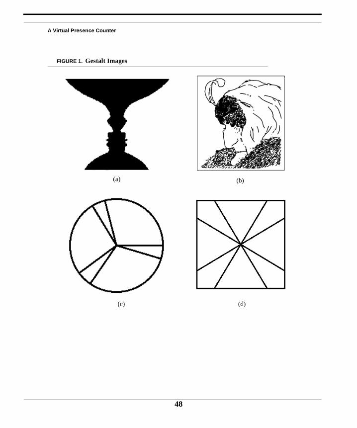
A Virtual Presence Counter
FIGURE 1. Gestalt Images
(a) (b)
(c) (d)
48
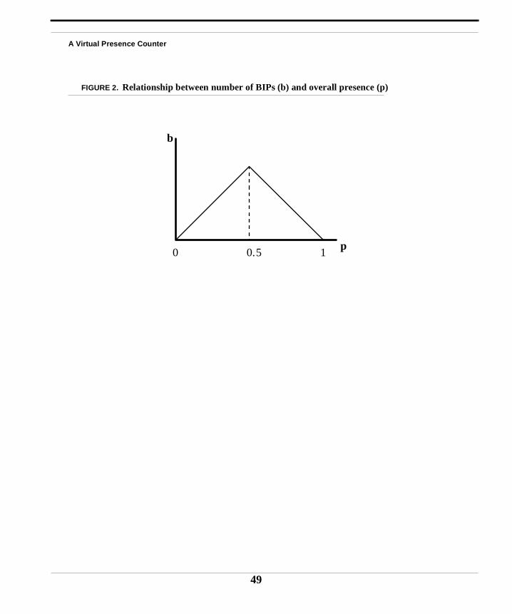
A Virtual Presence Counter
FIGURE 2. Relationship between number of BIPs (b) and overall presence (p)
0 1 p
b
0.5
49
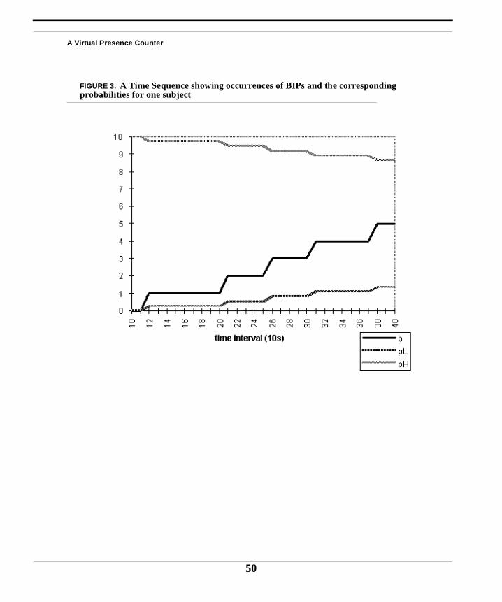
A Virtual Presence Counter
FIGURE 3. A Time Sequence showing occurrences of BIPs and the corresponding probabilities for one subject
50
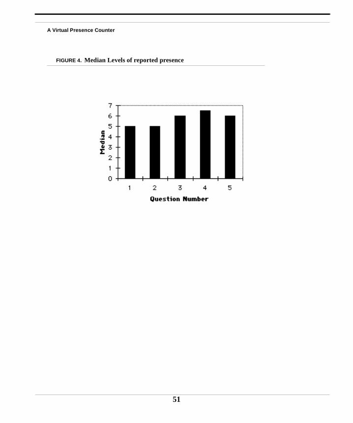
A Virtual Presence Counter
FIGURE 4. Median Levels of reported presence
51
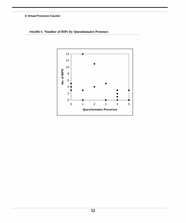
A Virtual Presence Counter
FIGURE 5. Number of BIPs by Questionnaire Presence
0
2
4
6
8
10
12
14
0 1 2 3 4 5
Questionnaire Presence
No
. of
BIP
S
52
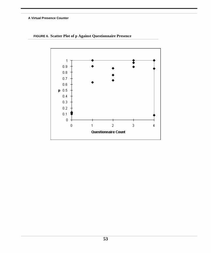
A Virtual Presence Counter
FIGURE 6. Scatter Plot of p Against Questionnaire Presence
53
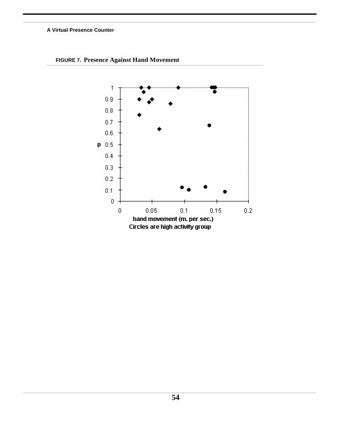
A Virtual Presence Counter
FIGURE 7. Presence Against Hand Movement
54