A very brief introduction to GRASS-GISusing the fishcamp dataset

Carlos Henrique Grohmann

guano@usp.br

Institute of Geosciences – USP – Brazil

Sao Paulo, September 6, 2011

Contents i

Contents

1 Introduction to GRASS-GIS 1

1.1 Design and structure . . . . . . . . . . . . . . . . . . . . . . . . . . . . . . . . 1

1.2 Organisation of projects . . . . . . . . . . . . . . . . . . . . . . . . . . . . . . 1

1.3 GRASS Tools – gism and Map Display . . . . . . . . . . . . . . . . . . . . . . 3

2 Defining a new Location and mapset 5

3 Importing data from fishcamp dataset 9

4 Exploring and analysing data in GRASS, working with regions 10

5 Interpolation, DEM creation 14

5.1 RST interpolation . . . . . . . . . . . . . . . . . . . . . . . . . . . . . . . . . 14

5.2 Direct DEM creation from LiDAR points . . . . . . . . . . . . . . . . . . . . 16

6 Morphometric parameters 17

6.1 Shaded Relief . . . . . . . . . . . . . . . . . . . . . . . . . . . . . . . . . . . . 17

6.2 Slope, Aspect, landscape features . . . . . . . . . . . . . . . . . . . . . . . . . 18

6.3 3D Visualisation . . . . . . . . . . . . . . . . . . . . . . . . . . . . . . . . . . 19

7 Running GRASS from R 20

7.1 Loading data from GRASS . . . . . . . . . . . . . . . . . . . . . . . . . . . . 20

7.2 Exploring the data . . . . . . . . . . . . . . . . . . . . . . . . . . . . . . . . . 23

8 Individual computer exercises 26

List of Figures

1.1 Organisation of GRASS data. After Dassau et al. (2005). . . . . . . . . . . 2

1.2 GRASS graphical user interface (Tcl/Tk). . . . . . . . . . . . . . . . . . . . 3

1.3 GIS Manager (gism) window. . . . . . . . . . . . . . . . . . . . . . . . . . . 4

1.4 GIS Manager upper toolbar. . . . . . . . . . . . . . . . . . . . . . . . . . . 4

1.5 GIS Manager lower toolbar. . . . . . . . . . . . . . . . . . . . . . . . . . . . 4

1.6 Map Display toolbar. . . . . . . . . . . . . . . . . . . . . . . . . . . . . . . 5

1.7 Map Display zoom options. . . . . . . . . . . . . . . . . . . . . . . . . . . . 5

2.1 Welcome to GRASS-GIS window. . . . . . . . . . . . . . . . . . . . . . . . 7

2.2 Select ‘Georeferenced File’. . . . . . . . . . . . . . . . . . . . . . . . . . . . 8

2.3 Select the file to be used. . . . . . . . . . . . . . . . . . . . . . . . . . . . . 8

2.4 Select the file to be used. . . . . . . . . . . . . . . . . . . . . . . . . . . . . 8

ii List of Tables

2.5 Select datum transformations parameters. . . . . . . . . . . . . . . . . . . . 9

2.6 Create a new mapset. . . . . . . . . . . . . . . . . . . . . . . . . . . . . . . 9

4.1 Add a new layer on the stack ans select a file to display . . . . . . . . . . . 11

4.2 Display the selected maps. . . . . . . . . . . . . . . . . . . . . . . . . . . . . 11

4.3 Display with map resolution of 2.5m (left) and with current region resolution

of 200m (right). . . . . . . . . . . . . . . . . . . . . . . . . . . . . . . . . . . 13

5.1 Query the vector map to find out which is the field to be used for interpolation. 15

5.2 DEM created from LiDAR points. The white areas are voids. . . . . . . . . 17

6.1 Original shaded relief map of lidar points 5m mean fill (left) and shaded map

of filetered DEM lidar fill 5x5avg diff fill (left) . . . . . . . . . . . . . . . . 18

6.2 Map of terrain features, calculated with a 13x13 moving-window . . . . . . 19

6.3 3D view of lidar fill 5x5avg diff fill . . . . . . . . . . . . . . . . . . 19

6.4 Terrain features drapped over DEM surface . . . . . . . . . . . . . . . . . . 20

7.1 Simple histogram of dem2m. . . . . . . . . . . . . . . . . . . . . . . . . . . . 24

7.2 Scatter plot of DEMNED03 and DEMSRTM1. . . . . . . . . . . . . . . . . . . . . 26

List of Tables

1.1 GRASS modules functions and classes . . . . . . . . . . . . . . . . . . . . . 1

1: Introduction to GRASS-GIS 1

1. Introduction to GRASS-GIS

GRASS1 (Geographic Resources Analysis Support System), is a raster/vector GIS com-

bined with image processing and data visualisation subsystems, it is one of the largest Free

Software GIS projects released under the GNU General Public License, and is one of the

founding projects of the Open Source Geospatial Foundation (OSGeo2) (Neteler & Mitasova,

2008).

1.1. Design and structure

Functions (modules) in GRASS are mainly oriented to raster or vector data types, with

additional modules for database management, file operations and image processing (orthorec-

tification, etc). There are over 350 modules in the base system, and the GRASS-wiki AddOns

page3 lists another hundred contributions from users.

The Command Line Interface (CLI) syntax of the modules follow a very simple structure.

All modules have a prefix that indicates its general class, and the name tries to be as self-

explanatory as possible (table 1.1).

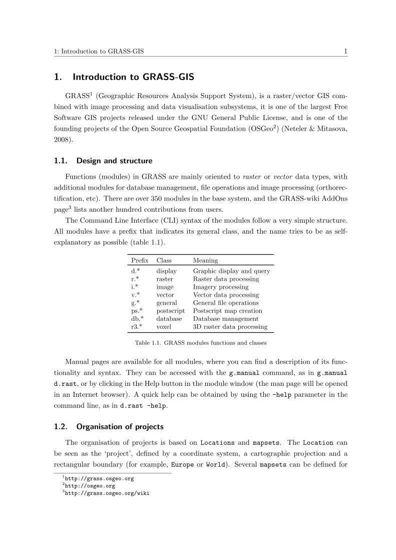
Prefix Class Meaning

d.* display Graphic display and queryr.* raster Raster data processingi.* image Imagery processingv.* vector Vector data processingg.* general General file operationsps.* postscript Postscript map creationdb.* database Database managementr3.* voxel 3D raster data processing

Table 1.1. GRASS modules functions and classes

Manual pages are available for all modules, where you can find a description of its func-

tionality and syntax. They can be accessed with the g.manual command, as in g.manual

d.rast, or by clicking in the Help button in the module window (the man page will be opened

in an Internet browser). A quick help can be obtained by using the -help parameter in the

command line, as in d.rast -help.

1.2. Organisation of projects

The organisation of projects is based on Locations and mapsets. The Location can

be seen as the ‘project’, defined by a coordinate system, a cartographic projection and a

rectangular boundary (for example, Europe or World). Several mapsets can be defined for

1http://grass.osgeo.org2http://osgeo.org3http://grass.osgeo.org/wiki

2 List of Tables

each Location. They can be seen either as ‘sub-projects’ (like Zurich, thesis data, etc) or

as a way to organize a multi-user project (like user1, user2, user3...).

Each Location must have at least one particular mapset, called PERMANENT (created

automatically with the Location). In a multi-user project, common data can (and should)

be stored in PERMANENT, since it is possible for several users to work at the same time in the

same Location, but not in the same mapset.

The projects are commonly placed in a directory (folder) that GRASS will call GISBASE

(usually /home/user/grassdata or C:\grassdata). The Locations will be sub-directories of

GISBASE, and each mapset will be a sub-directory of its Location.

All data must have the same coordinate system, projection and datum, as there is no

‘on-the-fly’ projection .

Each data layer requires several files (for geometry, attribute table, etc), and these files

are (so far) stored in different sub-directories inside the mapset, file management operations

(copy, rename, delete) must use the appropriate modules (g.copy, g.rename, g.remove).

Figure 1.1. Organisation of GRASS data. After Dassau et al. (2005).

The REGION is a key concept in GRASS, as it defines the boundaries and the spatial

resolution for operations on raster maps. Every raster map has its own extent and resolution

(defined in its header), but all raster operations will be performed using the extents and

resolution of the ‘active’ (or current) region. If the active region is smaller than the raster,

1.3 GRASS Tools – gism and Map Display 3

the operation will be performed only in the subset defined by the region, and if the spatial

resolution is different, the raster will be resampled automatically (by nearest neighbours).

It is very easy to change the extents and/or resolution of the active region, as well

as it is possible to save these settings and retrieve them when necessary, using the com-

mand g.region. Remember that the configurations of the active region does not necessarily

matches those of the Display.

1.3. GRASS Tools – gism and Map Display

Figure 1.2 shows the components of the GRASS Tcl/Tk Graphical User Interface (GUI).

The GIS Manager, or simply gism, is where the we found all the commands, separated in

menus and with some of them placed in toolbars. The area below the toolbars is where

we stack the data layers, like raster and vector data, colour composites (RGB or IHS) and

cartographic elements (like scalebars and north arrow). Note that the vertical stacking of the

layers will dictate the order of drawing in the display.

Figure 1.2. GRASS graphical user interface (Tcl/Tk).

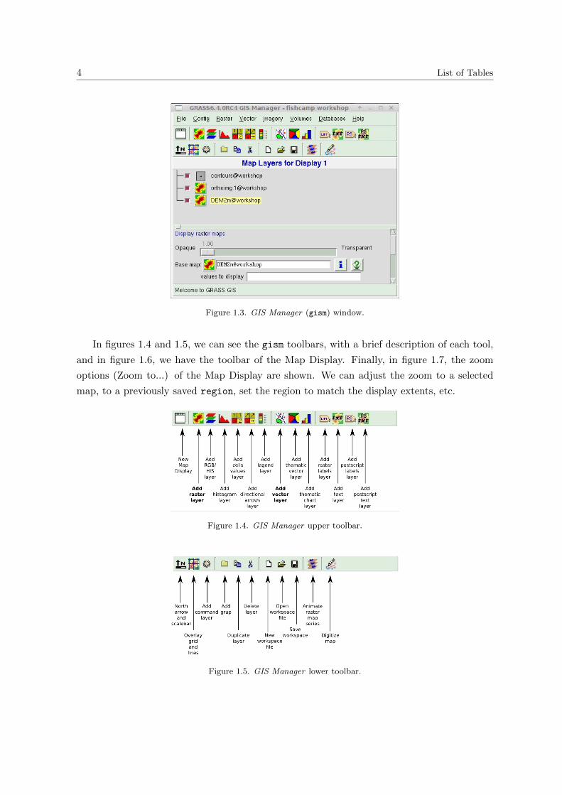
In the lower area of gism there are several options of exhibition according to the map

type. In figure 1.3, we can see some options for raster maps, as opacity, which map will be

displayed (Base Map) and which interval of values to display. the ‘i’ button next to map

name will provide general information about the layer in the output window (it is a shortcut

to r.info).

4 List of Tables

Figure 1.3. GIS Manager (gism) window.

In figures 1.4 and 1.5, we can see the gism toolbars, with a brief description of each tool,

and in figure 1.6, we have the toolbar of the Map Display. Finally, in figure 1.7, the zoom

options (Zoom to...) of the Map Display are shown. We can adjust the zoom to a selected

map, to a previously saved region, set the region to match the display extents, etc.

Figure 1.4. GIS Manager upper toolbar.

Figure 1.5. GIS Manager lower toolbar.

2: Defining a new Location and mapset 5

Figure 1.6. Map Display toolbar.

Figure 1.7. Map Display zoom options.

2. Defining a new Location and mapset

The first thing to do when working on GRASS, is to create a new Location and at least

one mapset. When you run the program for the time, you should see the following message

in the terminal window. Just hit <Enter> and you will get the light-green window as in

figure 2.1. If you use Windows, remember to start GRASS from Command Line, or else it

won’t be possible to run R from within GRASS.

guano[~]$ grass64

WELCOME TO GRASS Version 6.4.0RC4 2009

1) Have at your side all available GRASS tutorials

2) When working on your location, the following materials

are extremely useful:

- A topo map of your area

- Current catalog of available computer maps

3) Check the GRASS webpages for feedback mailinglists and more:

http://www.grass-gis.org

http://grass.osgeo.org

Hit RETURN to continue

6 List of Tables

Figure 2.1. Welcome to GRASS-GIS window.

In figure 2.1, the upper central field is the path to the GISBASE directory, the left lower

field lists the available Locations and in the lower central field lists the mapsets. The three

buttons in the lower right allow us to create a Location/mapset in different ways. With

‘Georeferenced File’, any regular georeferenced file (like a shapefile or a geotiff) can be used

to define the necessary values (coordinate system, datum, etc). With ‘EPSG codes’, we can

use pre-defined codes created by the European Petroleum Survey Group (EPSG) for several

combinations of datums/cartographic projections, and with ‘Projection values’ we need to

enter each parameter manually.

Click on the first button (fig. 2.2). You should get a window like in figure 2.3. Browse to

select a georeferenced file. In the example, I used the file contours.shp, from the fishcamp

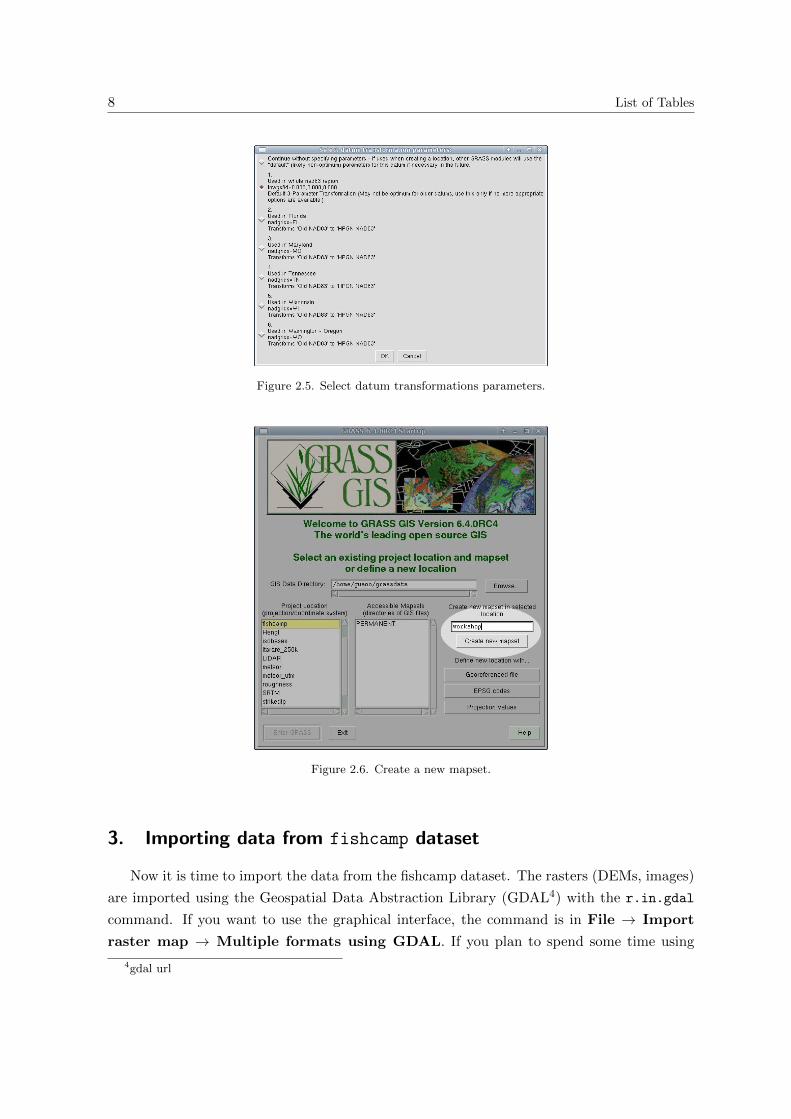
dataset (fig. 2.4). After selecting the file, you will need to decide on datum transformations

parameters (fig. 2.5). Select the number 1. You will be redirected to the ‘Welcome’ window,

where you should create a new mapset (workshop, in fig 2.6). After creating everything,

select the Location fishcamp, the mapset workshop and click on ‘Enter GRASS’.

2: Defining a new Location and mapset 7

Figure 2.2. Select ‘Georeferenced File’.

Figure 2.3. Select the file to be used.

Figure 2.4. Select the file to be used.

8 List of Tables

Figure 2.5. Select datum transformations parameters.

Figure 2.6. Create a new mapset.

3. Importing data from fishcamp dataset

Now it is time to import the data from the fishcamp dataset. The rasters (DEMs, images)

are imported using the Geospatial Data Abstraction Library (GDAL4) with the r.in.gdal

command. If you want to use the graphical interface, the command is in File → Import

raster map → Multiple formats using GDAL. If you plan to spend some time using

4gdal url

4: Exploring and analysing data in GRASS, working with regions 9

GRASS+R or if you plan to do some scripting to automate some processes, it is a good idea

to get used to the Command Line Interface (CLI). The commands looks like these:

r.in.gdal -o input=/home/guano/Zurich2009/fishcamp/DEM2m.asc output=DEM2m

r.in.gdal -o input=/home/guano/Zurich2009/fishcamp/DEMNED03.asc output=DEMNED03

r.in.gdal -o input=/home/guano/Zurich2009/fishcamp/DEMSRTM1.asc output=DEMSRTM1

r.in.gdal -o input=/home/guano/Zurich2009/fishcamp/orthoimg.lan output=orthoimg

The ‘-o’ option tells to r.in.gdal to overrride the file projection and to use the Location

projection. This is generally used when you know what is the projection of the file, but the

file doesn’t have a header or a .prj associate file (or just when you don’t care much).

The vector files are imported with v.in.ogr. OGR is part of the GDAL library. Here the

‘dsn’ means the directory where the files are, not the file themselves.

v.in.ogr dsn=/home/guano/Zurich2009/fishcamp/ output=lidar layer=lidar \

min_area=0.0001 snap=-1

v.in.ogr dsn=/home/guano/Zurich2009/fishcamp/ output=streams layer=streams \

min_area=0.0001 snap=-1

v.in.ogr dsn=/home/guano/Zurich2009/fishcamp/ output=contours layer=contours \

min_area=0.0001 snap=-1

4. Exploring and analysing data in GRASS, working with regions

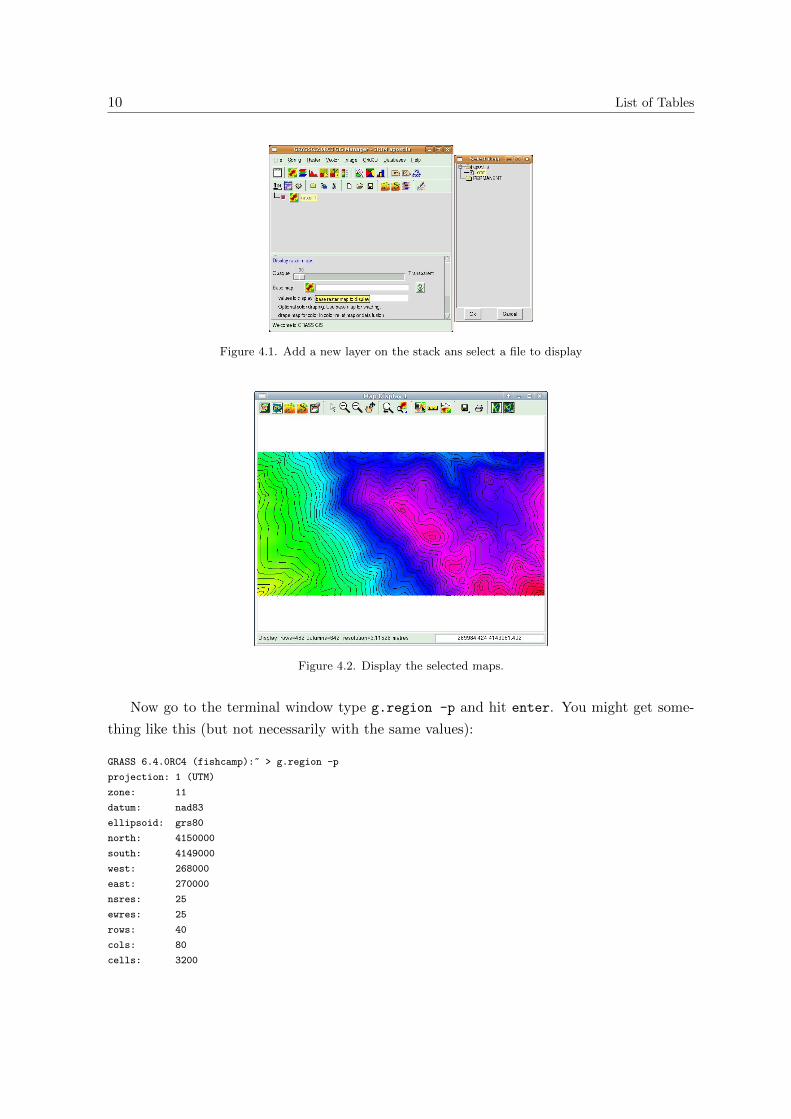
Now that the data was imported, try to visualise it. Click on ‘Add raster’ on gism, then

on the lower panel, click on the raster icon next to the name field, and you should get a

window to select the layer you want (fig. 4.1. Then, go to the Map Display and click Zoom

to...→ Zoom to selected map. In figure 4.2, you see the DEM2m raster overlaid by the

contours vector.

Play a little bit with it. Change the vertical order of the layer in gism, turn layers on an

off (the red square left to the layer’s name). Every time you change something, click on the

second button of the Map Display toolbar, to redraw all the layers.

10 List of Tables

Figure 4.1. Add a new layer on the stack ans select a file to display

Figure 4.2. Display the selected maps.

Now go to the terminal window type g.region -p and hit enter. You might get some-

thing like this (but not necessarily with the same values):

GRASS 6.4.0RC4 (fishcamp):~ > g.region -p

projection: 1 (UTM)

zone: 11

datum: nad83

ellipsoid: grs80

north: 4150000

south: 4149000

west: 268000

east: 270000

nsres: 25

ewres: 25

rows: 40

cols: 80

cells: 3200

4: Exploring and analysing data in GRASS, working with regions 11

The ‘-p’ flag tell g.region to print the current regions settings. We can see the coordinates

of the boundaries, the spatial resolution (25 m), the number of columns and rows, etc. Try

to change the spatial resolution:

GRASS 6.4.0RC4 (fishcamp):~ > g.region -p res=2.5

projection: 1 (UTM)

zone: 11

datum: nad83

ellipsoid: grs80

north: 4150000

south: 4149000

west: 268000

east: 270000

nsres: 2.5

ewres: 2.5

rows: 400

cols: 800

cells: 320000

GRASS 6.4.0RC4 (fishcamp):~ >

To see the effect that this change has on the maps, you need to set your Map Display to

adjust itself according to the current region (the default is to draw the map according to its

resolution). Just click on the next-to-last button of the Map Display toolbar.

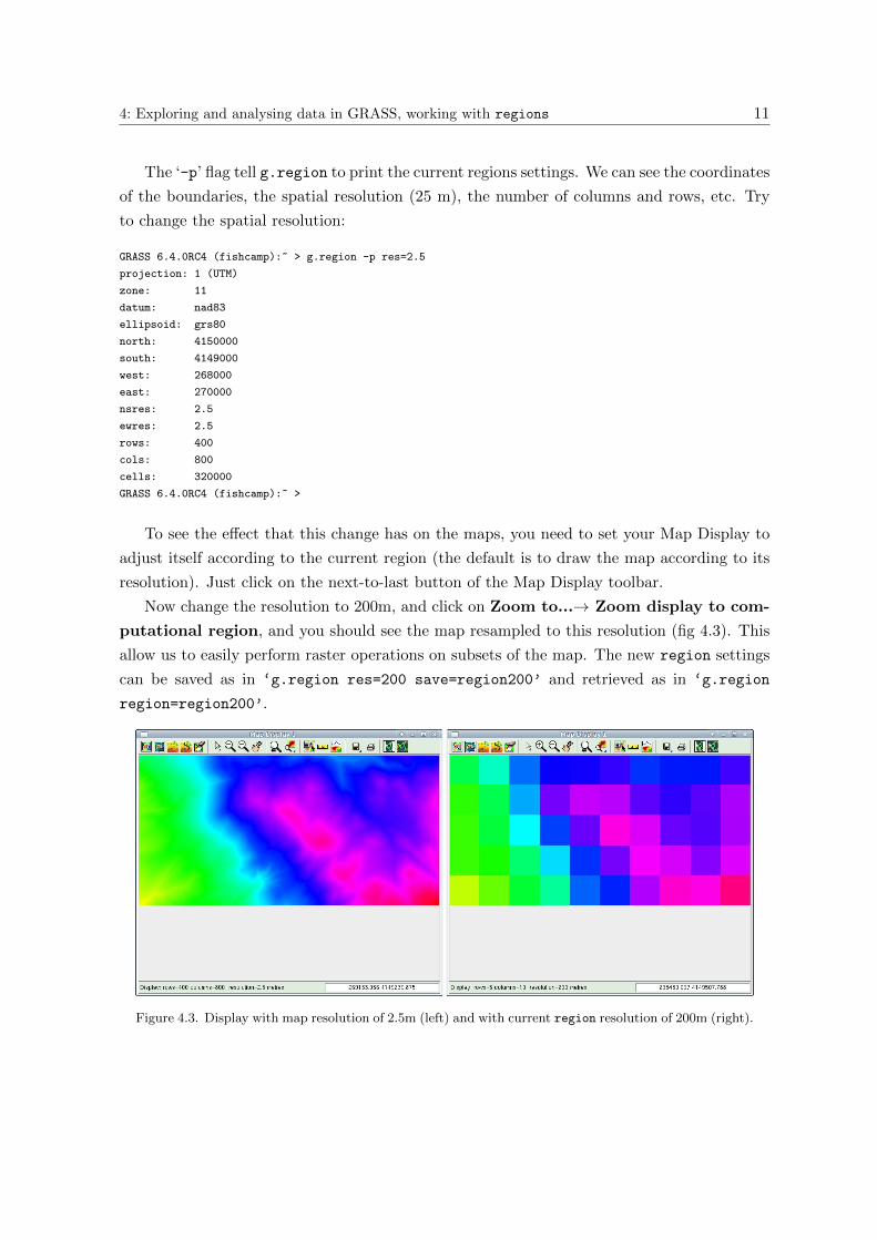
Now change the resolution to 200m, and click on Zoom to...→ Zoom display to com-

putational region, and you should see the map resampled to this resolution (fig 4.3). This

allow us to easily perform raster operations on subsets of the map. The new region settings

can be saved as in ‘g.region res=200 save=region200’ and retrieved as in ‘g.region

region=region200’.

Figure 4.3. Display with map resolution of 2.5m (left) and with current region resolution of 200m (right).

12 List of Tables

You can also change the limits of the region:

GRASS 6.4.0RC4 (fishcamp):~ > g.region -p n=4149900 s=4149100 w=268500 e=269500 res=10

projection: 1 (UTM)

zone: 11

datum: nad83

ellipsoid: grs80

north: 4149900

south: 4149100

west: 268500

east: 269500

nsres: 10

ewres: 10

rows: 80

cols: 100

cells: 8000

GRASS 6.4.0RC4 (fishcamp):~ >

And you can easily set the region to match a raster or vector layer:

GRASS 6.4.0RC4 (fishcamp):~ > g.region -p rast=DEM2m

projection: 1 (UTM)

zone: 11

datum: nad83

ellipsoid: grs80

north: 4150000

south: 4149000

west: 268000

east: 270000

nsres: 2.5

ewres: 2.5

rows: 400

cols: 800

cells: 320000

GRASS 6.4.0RC4 (fishcamp):~ >

All this region operations can be done in graphical mode.The command is at: Config →Region → Change region settings. Also, if you just type g.region in the command line

and hit enter, the graphical window for the command will show up (as well as for any other

command).

5. Interpolation, DEM creation

5.1. RST interpolation

Let’s try some interpolation and DEM creation. First, adjust the region settings to the

limits of the other rasters and with a resolution of 25m: g.region -p rast=DEM2m res=25

Now open the command v.surf.rst, which is used to interpolate smooth surfaces from

vector data (points or contours) using Regularized Splines with Tension (Mitasova & Mitas,

5.1 RST interpolation 13

1993; Mitasova & Hofierka, 1993). The module is at Raster → Interpolate surfaces →Regularized Spline Tension.

There are several options you can adjust for this module, but we will use the default values

for now. Also, you can choose to output not only the interpolated surface, but also the slope,

aspect, curvatures, etc. In the first tab of the module window (Parameters), the field we are

interested is the ‘Name of the attribute column with values to be used for approximation’

(zcolumn). This is the column of the data table associated with the vector map that contains

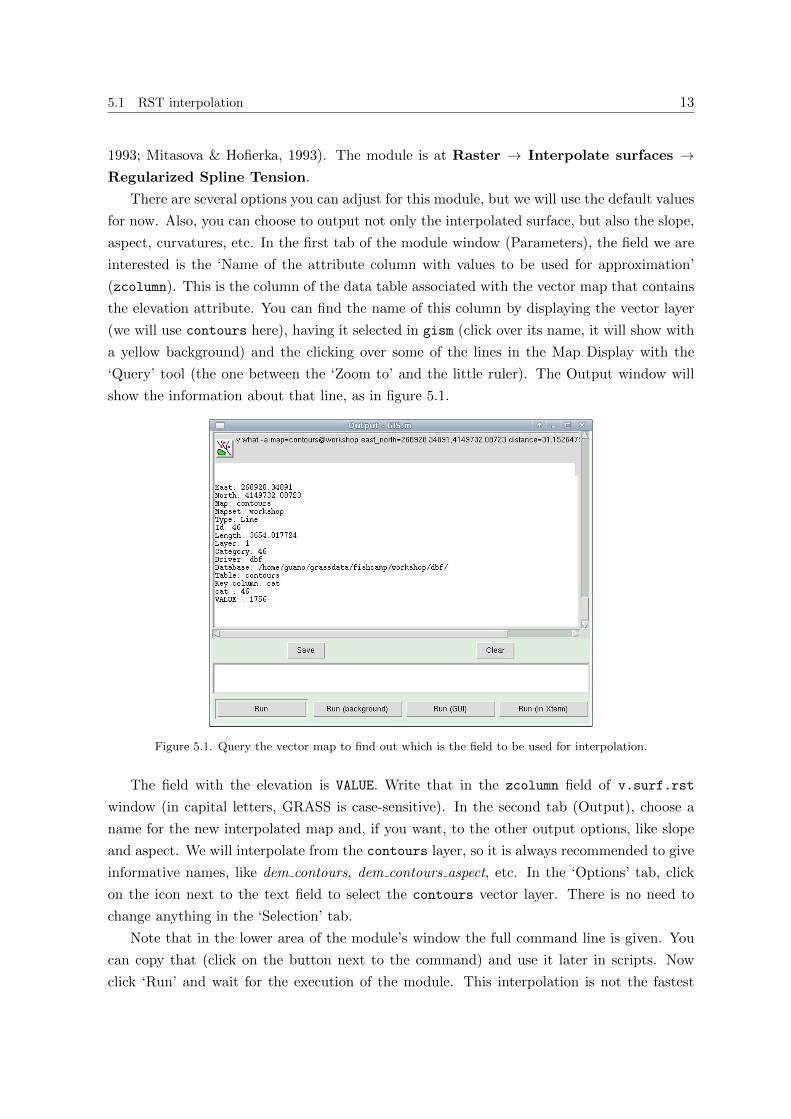
the elevation attribute. You can find the name of this column by displaying the vector layer

(we will use contours here), having it selected in gism (click over its name, it will show with

a yellow background) and the clicking over some of the lines in the Map Display with the

‘Query’ tool (the one between the ‘Zoom to’ and the little ruler). The Output window will

show the information about that line, as in figure 5.1.

Figure 5.1. Query the vector map to find out which is the field to be used for interpolation.

The field with the elevation is VALUE. Write that in the zcolumn field of v.surf.rst

window (in capital letters, GRASS is case-sensitive). In the second tab (Output), choose a

name for the new interpolated map and, if you want, to the other output options, like slope

and aspect. We will interpolate from the contours layer, so it is always recommended to give

informative names, like dem contours, dem contours aspect, etc. In the ‘Options’ tab, click

on the icon next to the text field to select the contours vector layer. There is no need to

change anything in the ‘Selection’ tab.

Note that in the lower area of the module’s window the full command line is given. You

can copy that (click on the button next to the command) and use it later in scripts. Now

click ‘Run’ and wait for the execution of the module. This interpolation is not the fastest

14 List of Tables

in the world, so it can take a while to process, depending on the number of data points (or

vertices of contour lines) and the spatial resolution of the current region.

We will compare this interpolated map with the SRTM DEM later, in R.

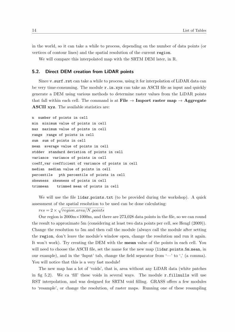
5.2. Direct DEM creation from LiDAR points

Since v.surf.rst can take a while to process, using it for interpolation of LiDAR data can

be very time-consuming. The module r.in.xyz can take an ASCII file as input and quickly

generate a DEM using various methods to determine raster values from the LiDAR points

that fall within each cell. The command is at File → Import raster map → Aggregate

ASCII xyz. The available statistics are:

n number of points in cell

min minimum value of points in cell

max maximum value of points in cell

range range of points in cell

sum sum of points in cell

mean average value of points in cell

stddev standard deviation of points in cell

variance variance of points in cell

coeff_var coefficient of variance of points in cell

median median value of points in cell

percentile pth percentile of points in cell

skewness skewness of points in cell

trimmean trimmed mean of points in cell

We will use the file lidar points.txt (to be provided during the workshop). A quick

assessment of the spatial resolution to be used can be done calculating:

res = 2×√region area/N points

Our region is 2000m×1000m, and there are 273,028 data points in the file, so we can round

the result to approximate 5m (considering at least two data points per cell, see Hengl (2009)).

Change the resolution to 5m and then call the module (always call the module after setting

the region, don’t leave the module’s window open, change the resolution and run it again.

It won’t work). Try creating the DEM with the mean value of the points in each cell. You

will need to choose the ASCII file, set the name for the new map (lidar points 5m mean, in

our example), and in the ‘Input’ tab, change the field separator from ‘—’ to ‘,’ (a comma).

You will notice that this is a very fast module!

The new map has a lot of ‘voids’, that is, area without any LiDAR data (white patches

in fig 5.2). We ca ‘fill’ these voids in several ways. The module r.fillnulls will use

RST interpolation, and was designed for SRTM void filling. GRASS offers a few modules

to ‘resample’, or change the resolution, of raster maps. Running one of these resampling

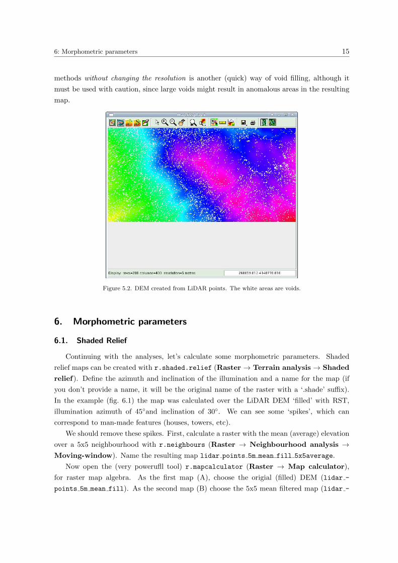
6: Morphometric parameters 15

methods without changing the resolution is another (quick) way of void filling, although it

must be used with caution, since large voids might result in anomalous areas in the resulting

map.

Figure 5.2. DEM created from LiDAR points. The white areas are voids.

6. Morphometric parameters

6.1. Shaded Relief

Continuing with the analyses, let’s calculate some morphometric parameters. Shaded

relief maps can be created with r.shaded.relief (Raster → Terrain analysis → Shaded

relief). Define the azimuth and inclination of the illumination and a name for the map (if

you don’t provide a name, it will be the original name of the raster with a ‘.shade’ suffix).

In the example (fig. 6.1) the map was calculated over the LiDAR DEM ‘filled’ with RST,

illumination azimuth of 45◦and inclination of 30◦. We can see some ‘spikes’, which can

correspond to man-made features (houses, towers, etc).

We should remove these spikes. First, calculate a raster with the mean (average) elevation

over a 5x5 neighbourhood with r.neighbours (Raster → Neighbourhood analysis →Moving-window). Name the resulting map lidar points 5m mean fill 5x5average.

Now open the (very powerufll tool) r.mapcalculator (Raster → Map calculator),

for raster map algebra. As the first map (A), choose the origial (filled) DEM (lidar -

points 5m mean fill). As the second map (B) choose the 5x5 mean filtered map (lidar -

16 List of Tables

points 5m mean fill 5x5average, in our example). Choose a name for the new map (like

lidar fill 5x5avg diff), and for the formula:

if(A-B>3.5,null(),A)

This means that if the difference between A and B is greater than 3.5m, the result will be

NULL (nodata), or else it will be the same as in map A. It is possible to create very complex

formulas with this module.

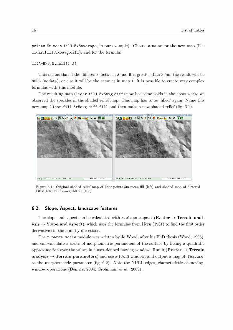
The resulting map (lidar fill 5x5avg diff) now has some voids in the areas where we

observed the speckles in the shaded relief map. This map has to be ‘filled’ again. Name this

new map lidar fill 5x5avg diff fill and then make a new shaded relief (fig. 6.1).

Figure 6.1. Original shaded relief map of lidar points 5m mean fill (left) and shaded map of fileteredDEM lidar fill 5x5avg diff fill (left)

6.2. Slope, Aspect, landscape features

The slope and aspect can be calculated with r.slope.aspect (Raster → Terrain anal-

ysis → Slope and aspect), which uses the formulas from Horn (1981) to find the first order

derivatives in the x and y directions.

The r.param.scale module was written by Jo Wood, after his PhD thesis (Wood, 1996),

and can calculate a series of morphometric parameters of the surface by fitting a quadratic

approximation over the values in a user-defined moving-window. Run it (Raster → Terrain

analysis → Terrain parameters) and use a 13x13 window, and output a map of ‘feature’

as the morphometric parameter (fig. 6.2). Note the NULL edges, characteristic of moving-

window operations (Demers, 2004; Grohmann et al., 2009).

6.3 3D Visualisation 17

Figure 6.2. Map of terrain features, calculated with a 13x13 moving-window

6.3. 3D Visualisation

GRASS offers a powerful N-dimensional visualisation tool, NVIZ. It is run from the third

button of the Map Display toolbar, and it will automatically load all the active layers in gism.

Try it by activating only the lidar fill 5x5avg diff fill raster and clicking in its button.

Since the very large number of calculations need to the 3D display, high spatial resolutions

will cause it to run slow. Change the resolution to 10 or 20m befor starting it.

Figure 6.3. 3D view of lidar fill 5x5avg diff fill

18 List of Tables

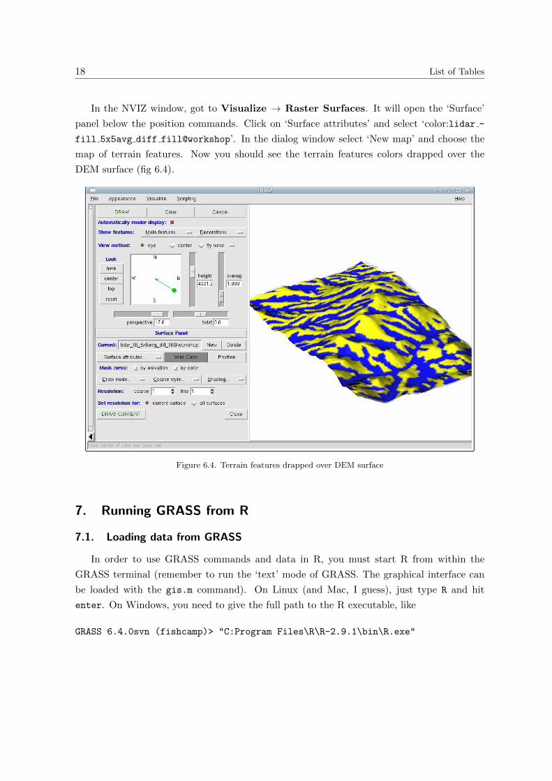
In the NVIZ window, got to Visualize → Raster Surfaces. It will open the ‘Surface’

panel below the position commands. Click on ‘Surface attributes’ and select ‘color:lidar -

fill 5x5avg diff fill@workshop’. In the dialog window select ‘New map’ and choose the

map of terrain features. Now you should see the terrain features colors drapped over the

DEM surface (fig 6.4).

Figure 6.4. Terrain features drapped over DEM surface

7. Running GRASS from R

7.1. Loading data from GRASS

In order to use GRASS commands and data in R, you must start R from within the

GRASS terminal (remember to run the ‘text’ mode of GRASS. The graphical interface can

be loaded with the gis.m command). On Linux (and Mac, I guess), just type R and hit

enter. On Windows, you need to give the full path to the R executable, like

GRASS 6.4.0svn (fishcamp)> "C:Program Files\R\R-2.9.1\bin\R.exe"

7.1 Loading data from GRASS 19

Once inside the R environment, load the spgrass6 ligrary:

> library(spgrass6)

Loading required package: sp

Loading required package: rgdal

Geospatial Data Abstraction Library extensions to R successfully loaded

Loaded GDAL runtime: GDAL 1.6.1, released 2009/05/11

Path to GDAL shared files: C:/PROGRA~1/R/R-29~1.1/library/rgdal/gdal

Loaded PROJ.4 runtime: Rel. 4.6.1, 21 August 2008

Path to PROJ.4 shared files: C:/PROGRA~1/R/R-29~1.1/library/rgdal/proj

Loading required package: XML

GRASS GIS interface loaded with GRASS version: 6.4.0svn

and location: fishcamp

>

The region settings can be obtained with the gmeta6() command:

> G<-gmeta6()

> G

gisdbase C:\grassdata

location fishcamp

mapset wshop

rows 1

columns 1

north 1

south 0

west 0

east 1

nsres 1

ewres 1

projection +proj=utm +no_defs +zone=11 +a=6378137 +rf=298.257222101

+towgs84=0.000,0.000,0.000 +to_meter=1

>

You can import maps to GRASS from R:

> system("r.in.gdal.exe -o input=C:/fishcamp/DEM2m.asc output=DEM2m")

WARNING: Over-riding projection check

100%

RINGDA~1 complete. Raster map <DEM2m> created.

Note that in Windows you must add the .exe suffix to the command. On linux it would

be:

> system("r.in.gdal -o input=/home/guano/Zurich2009/fishcamp/DEM2m.asc output=DEM2m")

20 List of Tables

> system("v.in.ogr.exe -o C:/fishcamp/contours.shp output=contours")

Over-riding projection check

Layer: contours

WARNING: Default driver / database set to:

driver: dbf

database: $GISDBASE/$LOCATION_NAME/$MAPSET/dbf/

Importing map 75 features...

-----------------------------------------------------

Building topology for vector map <contours>...

Registering primitives...

75 primitives registered

2555 vertices registered

Building areas...

100%

0 areas built

0 isles built

Attaching islands...

Attaching centroids...

100%

Number of nodes: 136

Number of primitives: 75

Number of points: 0

Number of lines: 75

Number of boundaries: 0

Number of centroids: 0

Number of areas: 0

Number of isles: 0

Now set the region to match the raster DEM2m:

> system("g.region.exe -p rast=DEM2m")

projection: 1 (UTM)

zone: 11

datum: nad83

ellipsoid: grs80

north: 4150000

south: 4149000

west: 268000

east: 270000

nsres: 2.5

ewres: 2.5

rows: 400

cols: 800

cells: 320000

7.2 Exploring the data 21

To load a raster map into R, use readRAST6(), and for vector, use readVECT6():

> dem2m <- readRAST6("DEM2m")

C:/grassdata/fishcamp/wshop/.tmp/DEM2m has GDAL driver GTiff

and has 400 rows and 800 columns

>

> contours <- readVECT6("contours")

Exporting 75 points/lines...

100%

75 features written

OGR data source with driver: ESRI Shapefile

Source: "C:/grassdata/fishcamp/wshop/.tmp", layer: "contours"

with 75 features and 2 fields

Feature type: wkbLineString with 2 dimensions

7.2. Exploring the data

Get some info about the raster:

> summary(dem2m)

Object of class SpatialGridDataFrame

Coordinates:

min max

x 268000 270000

y 4149000 4150000

Is projected: TRUE

proj4string :

[+proj=utm +no_defs +zone=11 +a=6378137 +rf=298.257222101

+towgs84=0.000,0.000,0.000 +to_meter=1]

Number of points: 2

Grid attributes:

cellcentre.offset cellsize cells.dim

x 268001.2 2.5 800

y 4149001.2 2.5 400

Data attributes:

Min. 1st Qu. Median Mean 3rd Qu. Max.

1402 1577 1703 1671 1759 1893

Try a histogram:

> hist(dem2m)

Error in hist.default(dem2m) : ’x’ must be numeric

Find out more about the raster:

22 List of Tables

> str(dem2m)

Formal class ’SpatialGridDataFrame’ [package "sp"] with 6 slots

..@ data :’data.frame’: 320000 obs. of 1 variable:

.. ..$ DEM2m: num [1:320000] 1549 1549 1549 1549 1548 ...

..@ grid :Formal class ’GridTopology’ [package "sp"] with 3 slots

.. .. ..@ cellcentre.offset: Named num [1:2] 268001 4149001

.. .. .. ..- attr(*, "names")= chr [1:2] "x" "y"

.. .. ..@ cellsize : num [1:2] 2.5 2.5

.. .. ..@ cells.dim : int [1:2] 800 400

..@ grid.index : int(0)

..@ coords : num [1:2, 1:2] 268001 269999 4149001 4149999

.. ..- attr(*, "dimnames")=List of 2

.. .. ..$ : NULL

.. .. ..$ : chr [1:2] "x" "y"

..@ bbox : num [1:2, 1:2] 268000 4149000 270000 4150000

.. ..- attr(*, "dimnames")=List of 2

.. .. ..$ : chr [1:2] "x" "y"

.. .. ..$ : chr [1:2] "min" "max"

..@ proj4string:Formal class ’CRS’ [package "sp"] with 1 slots

.. .. ..@ projargs: chr " +proj=utm +no_defs +zone=11 +a=6378137 +rf=298.25722

2101 +towgs84=0.000,0.000,0.000 +to_meter=1"

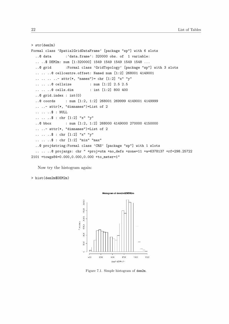
Now try the histogram again:

> hist(dem2m$DEM2m)

Figure 7.1. Simple histogram of dem2m.

7.2 Exploring the data 23

Import the DEMNED03 and DEMSRTM1 rasters (set the region settings to match the SRTM

DEM, so the NED DEM will be resampled and both maps will have the same number of cells)

and check the correlation between them:

> system("g.region.exe -p rast=DEMSRTM1")

projection: 1 (UTM)

zone: 11

datum: nad83

ellipsoid: grs80

north: 4150000

south: 4149000

west: 268000

east: 270000

nsres: 25

ewres: 25

rows: 40

cols: 80

cells: 3200

> srtm <- readRAST6("DEMSRTM1")

C:/grassdata/fishcamp/wshop/.tmp/DEMSRTM1 has GDAL driver GTiff

and has 40 rows and 80 columns

> ned <- readRAST6("DEMNED03")

C:/grassdata/fishcamp/wshop/.tmp/DEMNED03 has GDAL driver GTiff

and has 40 rows and 80 columns

>

> linmod <- lm(srtm$DEMSRTM1~ned$DEMNED03)

> linmod

Call:

lm(formula = srtm$DEMSRTM1 ~ ned$DEMNED03)

Coefficients:

(Intercept) ned$DEMNED03

60.2539 0.9738

> plot(srtm$DEMSRTM1~ned$DEMNED03)

> abline(linmod)

>

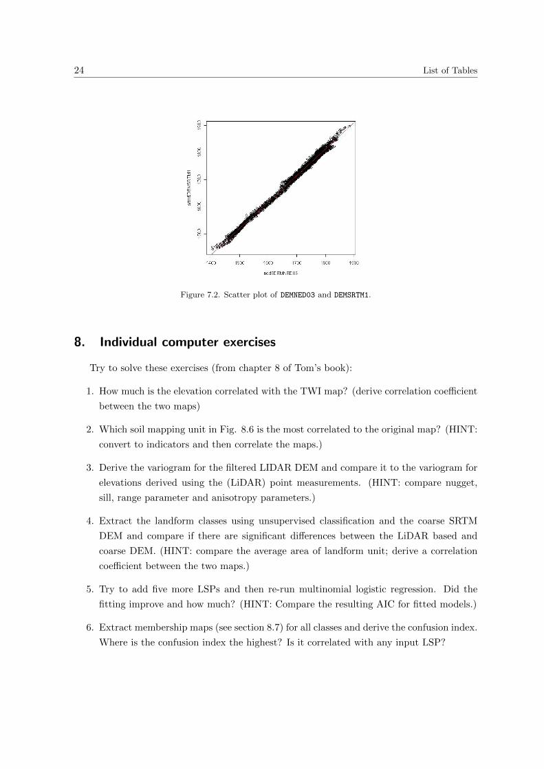
24 List of Tables

Figure 7.2. Scatter plot of DEMNED03 and DEMSRTM1.

8. Individual computer exercises

Try to solve these exercises (from chapter 8 of Tom’s book):

1. How much is the elevation correlated with the TWI map? (derive correlation coefficient

between the two maps)

2. Which soil mapping unit in Fig. 8.6 is the most correlated to the original map? (HINT:

convert to indicators and then correlate the maps.)

3. Derive the variogram for the filtered LIDAR DEM and compare it to the variogram for

elevations derived using the (LiDAR) point measurements. (HINT: compare nugget,

sill, range parameter and anisotropy parameters.)

4. Extract the landform classes using unsupervised classification and the coarse SRTM

DEM and compare if there are significant differences between the LiDAR based and

coarse DEM. (HINT: compare the average area of landform unit; derive a correlation

coefficient between the two maps.)

5. Try to add five more LSPs and then re-run multinomial logistic regression. Did the

fitting improve and how much? (HINT: Compare the resulting AIC for fitted models.)

6. Extract membership maps (see section 8.7) for all classes and derive the confusion index.

Where is the confusion index the highest? Is it correlated with any input LSP?

References 25

References

Dassau, O., Holl, S., Neteler, M., & Redslob, M., 2005. An introduction to the practical use of the

Free Geographical Information System GRASS 6.0. GDF Hannover bR.

Demers, M. N., 2004. Fundamentals of Geographic Information Systems. John Wiley & Sons, New

York.

Grohmann, C. H., Smith, M. J., & Riccomini, C., 2009. Surface Roughness of Topography: A Multi-

Scale Analysis of Landform Elements in Midland Valley, Scotland. In: Purves, R., Gruber, S., Hengl,

T., & Straumann, R., (Eds.), Proceedings of Geomorphometry2009, p. 140–148, Zurich, Switzerland.

Hengl, T., 2009. A Practical Guide to Geostatistical Mapping of Environmental Variables. EUR

22904 EN - 2007. European Commission – Joint Research Centre Institute for Environment and

Sustainability, 2nd edition.

Horn, B. K. P., 1981. Hill Shading and the Reflectance Map. Proceedings of the IEEE, 69:14–47.

Mitasova, H. & Hofierka, J., 1993. Interpolation by regularized spline with tension:II. Application to

terrain modeling and surface geometry analysis. Mathematical Geology, 25:657–669.

Mitasova, H. & Mitas, L., 1993. Interpolation by regularized spline with tension:I Theory and imple-

mentation. Mathematical Geology, 25:641–655.

Neteler, M. & Mitasova, H., 2008. Open Source GIS : A GRASS GIS Approach, Third Edition (The

International Series in Engineering and Computer Science), volume 773. Springer, New York.

Wood, J., 1996. The Geomorphological characterization of Digital Elevation Models. Tese de

Doutorado, University of Leicester, U. K. , Department of Geography, PhD Thesis.