a universal hurricane frequency function
TRANSCRIPT
7/29/2019 A Universal Hurricane Frequency Function
http://slidepdf.com/reader/full/a-universal-hurricane-frequency-function 1/29
A Universal Hurricane Frequency Function
Robert Ehrlich
George Mason University, Fairfax, VA
December 28, 2009
__________________
Corresponding author address: Robert Ehrlich, Physics & Astronomy Department, George Mason
University, Fairfax, VA 22030.
E-mail: [email protected]
ABSTRACT
Evidence is provided that the global distribution of tropical hurricanes is principally
determined by a universal function H of a single variable z that in turn is expressible in
terms of the local sea surface temperature and latitude. The data-driven model presented
here carries stark implications for the large increased numbers of hurricanes which it

7/29/2019 A Universal Hurricane Frequency Function
http://slidepdf.com/reader/full/a-universal-hurricane-frequency-function 2/29
2
predicts for a warmer world. Moreover, the rise in recent decades in the numbers of
hurricanes in the Atlantic, but not the Pacific basin, is shown to have a simple
explanation in terms of the specific form of H(z), which yields larger percentage
increases when a fixed increase in sea surface temperature occurs at higher latitudes and
lower temperatures.

7/29/2019 A Universal Hurricane Frequency Function
http://slidepdf.com/reader/full/a-universal-hurricane-frequency-function 3/29
3
1. Introduction
There are numerous factors that either promote or inhibit the formation of hurricanes or
tropical storms, and it is well-known that two of them have special significance: the sea
surface temperature SST (or simply T) and the latitude at the time and place of storm
formation. The importance of latitude is that it governs the strength of the Coriolis
Effect, a principal factor in creating some initial vorticity, while the SST is the source of
an updraft of air that can create a tropical low. Here, we assert more specifically that the
probability density of a hurricane or tropical storm forming can be expressed in terms of
a simple mathematical function of those two variables, ),( T H . Alternatively, we can
even write H in terms of a single combined variable ||sin)( 2/1
0 T T z , where T is
the SST, T0 is a threshold value of 25.50C, and is the latitude. The functional form of
H(z) most consistent with the data is found to be a simple power law, H(z) = Czn, where
C = 0.00073, and n = 3.5+0.5, for most regions of the globe. This result appears to be
independent of time, and location, with the exception of those regional departures.
The study reported here rests on four key assumptions.
a. Existence
There exists a probability function H which describes whether a hurricane (also referred
to as a cyclone or typhoon) forms. Furthermore, we assume that H depends on numerous
variables, of which only the SST and the latitude play a universal role, with the other
``secondary" variables, being restricted in time or space.
7/29/2019 A Universal Hurricane Frequency Function
http://slidepdf.com/reader/full/a-universal-hurricane-frequency-function 4/29
4
b. Secondary variables
The secondary variables influencing H do so in a way that simply multiplies it by a
constant factor that is regionally and temporally limited, and can be explained in terms of
previously studied regional or oscillatory phenomena that enhance the value of H by a
specific factor over that spatial or temporal region.
c. Data-driven
The function H can be found using the data on recorded hurricanes, without requiring a
fundamental understanding of the basic physics describing exactly how a hurricane
forms. This latter subject is one of current research interest, and the clue offered by the
specific functional form of H presented here may advance that search for understanding.
Since the function H is justified by appealing to data rather than fundamental theory, the
result is a model rather than a theory.
d. Validation
Given a specific form of H derived from the data, we can test the model by cross-
checking it for consistency using the data, and more importantly, by seeing whether
future hurricane data agrees with the model.

7/29/2019 A Universal Hurricane Frequency Function
http://slidepdf.com/reader/full/a-universal-hurricane-frequency-function 5/29
5
2. Methods
This work has relied on the data sets maintained by NOAA for the Atlantic and Eastern
Pacific regions, and by the Joint Typhoon Warning Center (JTWC) Task Force of the
U.S. Navy and Air Force for the World's other oceans. These data sets show both the
reconstructed SST by month in 20
x 20
latitude-longitude bins for each month from 1854
to the present, and the tracks of tropical storms and hurricanes occurring over the period
1945 to the present for storms in the Western (Asian) Pacific and Indian Oceans,
including the Southern Hemisphere, as well as those of Atlantic and Eastern Pacific. For
the present study we focus only on the latitude-longitude location for the first point on the
track of each storm (assumed to be its point of origin), and we have included both
tropical storms as well as hurricanes, which we henceforth do not distinguish.
The era of meteorological satellites began in the early 1960's, so it might be expected that
geographic distributions of points of origin of tropical storms would be less biased for
storms recorded since 1960 -- a suggestion which is confirmed by the observed
depopulation of storms in regions far from shipping lanes of Atlantic storms before 1960
compared to later ones. Thus, in order to use a data set that is not clearly biased in terms
of geographic distribution, we only use storms since 1960 in finding H(z).
Tropical storms can be thought of as heat engines which derive their energy from the
warm surface temperature of the ocean -- or more precisely the temperature difference
between the warm ocean and the much lower temperature at high altitude in the
7/29/2019 A Universal Hurricane Frequency Function
http://slidepdf.com/reader/full/a-universal-hurricane-frequency-function 6/29
6
atmosphere, which can represent a differential of around 1000C. It has been observed
that tropical storms do not arise unless the SST, T, exceeds some threshold value T0 cited
in various sources as being 26 or 270C. The other key variable in storm formation besides
SST is the latitude, which is important because the horizontal component of the Coriolis
force varies as its sine. The Coriolis force produces some initial vorticity that helps the
storm self-organize. Thus, tropical storms do not form very close to the equator, and they
have opposite senses of rotation in the two hemispheres.
In searching for a function H, we make use of the above well-known aspects of tropical
storm formation, and hence assume that the relevant variables entering the distribution H
involve the quantities 0T T and sin . Since it is much easier searching an unknown
function of a single variable than one involving two variables, we divide the search
process into two steps: first, finding a single combined variable z expressed in terms of
0T T and sin and second finding an appropriate functional form of z that best fits the
data. One plausible combination of the variables when 00 T T is
||sin)( 0 baT T z , which vanishes when either 0T T and 0 , although one
might well imagine other possible choices. The second part of the search for the form of
the function can be done visually by trial and error (for any given trial values of a and b)
because we want the resulting H(z) generated using the data themselves to satisfy these
six requirements:
7/29/2019 A Universal Hurricane Frequency Function
http://slidepdf.com/reader/full/a-universal-hurricane-frequency-function 7/29
7
a. Threshold
H (z) must have the correct threshold behavior. This requirement is guaranteed by our
choice of z for all a and b, as long as H(z) vanishes when z approaches zero.
b. Symmetry
H (z) must be a symmetrical function between the hemispheres even though the actual
numbers of storms is not symmetric.
c. Monotonicity
H (z) must be a monotonic function of z since we expect H to increase continually as
either 0T T or increase – although we cannot rule out a priori the possibility that it
levels off at some saturation value for large z.
d. Uniformity
H (z) must have the same functional form in each basin across the globe.
e. Normalization
H(z) ideally should also have the same normalization in each basin, or if not, the
variations should be explainable in terms of known regional phenomena.
f. Zeroes
H(z) must not predict storms occurring in any regions of the globe where none are
observed, e.g., in the South Atlantic.

7/29/2019 A Universal Hurricane Frequency Function
http://slidepdf.com/reader/full/a-universal-hurricane-frequency-function 8/29
8
Let us now explain exactly how H(z) is deduced from the data themselves. The point of
origin of each recorded storm in the data base places it in a specific latitude-longitude cell
(taken here to be 4 x 4 degrees), and since the time of occurrence of that storm is known,
we can use the SST-record to find the T in that cell when the storm formed. Given a
particular trial definition relating z to T and , we can then compute the z-value
associated with each storm. The z-values are binned, and we simply count the number of
storms N j in the jth bin between z j and z j+1. We then use the SST-record to obtain T for a
given month for each latitude-longitude cell to find the number of months during the 47-
year record from 1960-2007 that a given cell had a temperature T. Finally combining
that T with the values of each cell, we find the number of months M j that cells in a
given geographic basin (such as the Atlantic) had a specific binned z-value, z j. The
computed value of H for that z j simply equals N j/M j, which represents the observed
number of storms per month in 4x4 degree latitude-longitude cells for a given z. Since
these numbers are always less than one, it is more appropriate to think of them as the
probability of having a storm per month. Once we have deduced from the data a set of
H-values with associated uncertainties (discussed later), we can proceed to find the
functional form of H based on a best fit to the data-derived values. Given the fairly
stringent requirements on the form of H(z) discussed earlier, the search for an H(z) that
fits the data is fairly easy, given any trial choice of a and b used to define the variable z.

7/29/2019 A Universal Hurricane Frequency Function
http://slidepdf.com/reader/full/a-universal-hurricane-frequency-function 9/29
9
For example, we have found that the simplest choice: ||sin)( 0 T T z is found to give
poor results, while the choice: ||sin)( 2/1
0 T T z , gives good ones as we shall see in
the next section. Based on chi square for the Asian Pacific basin the best fitting exponent
b in ||sin)( 0 baT T z is actually b=0.49 +0.01.) One interesting property of our
choice of ||sin)(0 baT T z is that it yields a common temperature threshold T0 for
all latitudes, which may seem surprising. Other possible choices such as
||sin)( 0 ba cT T z would not have this feature, but they would introduce one
more free parameter, and would imply that H(z) is no longer separable into functions of T
and . Were our choice not found to yield a good fit to the data, one would need to
explore such more complex definitions of z.
3. Results
In order to test how well the data from various regions of the world agree with a power
law in z, i.e., ||sin)()( 2/
0 nnn T T Cz z H , we have relied heavily on the data for
the Asian Pacific basin. These data constrain H(z) far more than Atlantic data, since (a)
the Asian Pacific basin includes over five times as many storms as the Atlantic basin, (b)
it includes storms over a larger range of latitudes (31 bins in z versus only 17 for Atlantic
data), and (c) the Asian Pacific includes appreciable numbers of storms in both
hemispheres, whereas fewer than 1% of Atlantic storms are in the Southern Hemisphere.
We show in fig. 1 H(z) values derived from the data for the Asian Pacific basin, where
we artificially display Southern Hemisphere data points as having negative z-values, so

7/29/2019 A Universal Hurricane Frequency Function
http://slidepdf.com/reader/full/a-universal-hurricane-frequency-function 10/29
10
as to demonstrate the degree of symmetry for the data-derived function H(z). The data
may be seen to agree well with a n=3.5 + 0.5 power law for H(z), with C= 0.00073+
.00006, and T0 = 25.50C. The chi square for the fit is 29.2 for 30 d.o.f. (P = 51 %).
Before discussing the quality of fit for data in the other hurricane basins, we digress to
consider the size of the error bars used in fig.1, which directly affects the quality of the
fits.
a. Size of Uncertainties
Although one often only displays error bars on the dependent variable only, here the
independent variable z also has a significant uncertainty that must be taken into account.
The former uncertainty arises because of the statistical errors inherent in the computation
of H for each data point. Thus, to find H we assume that N j and M j are uncertain by
j N , and j M respectively, yielding for M H H H /)1( . The uncertainty in
the independent variable z is not merely + 0.05, as might be expected based on half the
bin width in z, but instead the larger value + 0.15. The reason for this enlargement of the
z-errors is that from the definition of ||sin)( 2/1
0 T T z , we see that because the data
is binned in 4 by 4 degree bins and also in increments of 0.250C in T, we need to use an
uncertainty (due to binning) of 02 and C T 0125.0 . When these errors are
propagated and added in quadrature to find the uncertainty in z using representative
values of T and for storms, we find that 15.0 z .

7/29/2019 A Universal Hurricane Frequency Function
http://slidepdf.com/reader/full/a-universal-hurricane-frequency-function 11/29
11
Finally, since the quantity H(z)/zn
should be a constant if H(z) satisfies a zn
power law,
we may use standard error propagation methods to find the variance in H(z)/zn
by
combining the separate uncertainties in z and H according to:
22
1
2
nn z
H z
z
nH
Note that it is this resultant uncertainty that is used to compute chi square under the
requirement that H(z)/zn remains constant, and thus:
2
22 )(1 C
z z H n
b. The Other Hurricane Basins
Let us now consider how well the data from other basins fits H(z), starting with the
Eastern Pacific, principally the region off the Southern coast of Mexico -- a region of
very frequent storms. This data (the filled triangles in fig. 2) appears to be at odds with
what was seen in the Western (Asian) Pacific basin in two important respects. First,
although most of the data again lies on a z3.5
power law (upper) curve, its normalization is
3.6 times higher than for the Western Pacific data. Second, three data points with the
largest z-values lie on the lower curve having the original normalization shown for fig. 1.
As it happens the Easter Pacific is one area significantly affected by the Madden-Julian
Oscillation (MJO). The MJO is a large-scale quasi-periodic modulation of tropical winds
that travels eastward from Asia to America. It has been previously shown that hurricane
activity in the Eastern Pacific is around four times more likely during the phase of the

7/29/2019 A Universal Hurricane Frequency Function
http://slidepdf.com/reader/full/a-universal-hurricane-frequency-function 12/29
12
oscillation associated with ascending rather than descending wind flows – see Maloney
(2000). Furthermore, the MJO oscillation leads to a significant modulation of the SST by
around 0.50C during the cycle, with the phase of the increased hurricane activity being
associated with a reduction in SST – see Maloney (2001} These preceding findings can
help explain the otherwise anomalous results of fig.2. Given that most storms in the
Eastern Pacific occur in a fairly narrow range of latitudes off the Southern coast of
Mexico, larger z values are equivalent to higher temperatures. We thus see that the three
filled triangle data points for the highest z-values are consistent with a H(z) = Cz3.5
, with
the original normalization observed for the Pacific data, while the data corresponding to
lower z-values are consistent with H(z) = 3.6Cz3.5
, given the effect of the MJO in
increasing hurricane formation approximately four-fold during the phase associated with
lower SST.
A similar regional effect must be invoked to explain the data in the Atlantic basin, for
which a narrow band of increased hurricane genesis can be observed between South
America and Africa at a latitude range of between 10 and 15 degrees North latitude. As
can be seen (open squares in fig. 2), the data in this band again lie on a n=3.5 power law
curve with the same factor of 3.6 enhancement that was found for the Eastern Pacific
data. As it happens, this narrow band of the Atlantic is during the summer a major
portion of the Intertropical Convergence Zone (ITCZ), where winds from the two
hemispheres converge, and it creates an area of low atmospheric pressure and the rapid
upward convection of moist air -- conditions which are conducive to the formation of
7/29/2019 A Universal Hurricane Frequency Function
http://slidepdf.com/reader/full/a-universal-hurricane-frequency-function 13/29
13
hurricanes. The remainder of the Atlantic basin away from this band is also consistent
with H(z) = Cz3.5
(chi square = 17.1 for 17 d.o.f), with the original normalization --
i.e., no factor of 3.6 multiplier. Thus, the data from all portions of the globe having
significant numbers of hurricanes are consistent with this same functional form, and even
the same normalization, provided one includes a factor of 3.6 enhancement in those
regions subject to constant or quasi periodic influences that have been found previously
to increase hurricane formation. Furthermore, the function H(z) does not predict any
storms should occur in regions of the globe where none are found.
c. Temporal Trends
The results presented until now all deal with the spatial distribution of hurricanes, and the
function H(z) was deduced with no direct reference to temporal variations -- except
through the correlation between local SST and time. The model can, however, be used to
predict temporal variations based on the SST of each latitude-longitude bin at any
given time. The procedure is to sum the fitted H(z) over all cells with a given z for that
particular time. Therefore, the model (if correct) should agree with the observed
temporal variations in numbers of storms over some extended time period. In what
follows, we make these comparisons with the data three different ways. One comparison
(figs. 3, and 4), shows the numbers of hurricanes predicted to occur each month of the
year (averaged over the period 1960-2007) by the model with those actually observed in

7/29/2019 A Universal Hurricane Frequency Function
http://slidepdf.com/reader/full/a-universal-hurricane-frequency-function 14/29
14
three particular basins: the North Asian Pacific, the Southern Hemisphere, and the
combined Atlantic and Eastern Pacific basins. In most cases the agreement is fairly good,
with the Southern Hemisphere probably being the worst. It should be noted that the
horizontal error bars extend 50% beyond the half-month associated with the bin width.
The reason for increasing these error bars is that it has been found that the process of
hurricane genesis from some initial disturbance has a tendency to cluster in time
sometimes over a period of several weeks. Gray (1979). Since we want to associate SST
with the very start of the process, not the observed first point on a hurricane track, we
therefore add an extra + 1 week uncertainty to the horizontal error bars.
A second temporal variation we may check is the year-to-year variation in numbers of
hurricanes in different basins. The poorest of the comparisons is that for the Asian
Pacific basin where the model shows a rise towards the end of the 47-year interval
1960-2007, while the data (fig. 5) shows almost no rise. The extent of the discrepancy
can be judged by a comparison of a quadratic fit to the model (dotted curve) that is
superimposed on the data. This discrepancy is bothersome, but it has not yet reached a
statistically significant level -- at least if one includes N statistical uncertainties in both
the data and the model. The chi square for the fit is a perfectly acceptable 38.0 for 47
d.o.f.) It must also be noted that the Asian basin data is much less reliable than the
Atlantic data in terms of time trends, especially for data prior to 1985, according Charles
Sampson who has made corrections to this data.-- Sampson (2008}.
7/29/2019 A Universal Hurricane Frequency Function
http://slidepdf.com/reader/full/a-universal-hurricane-frequency-function 15/29
15
In contrast to the Pacific time trend, that for the Atlantic basin agrees very well with the
model. Even though the Atlantic data pre-1960 may have missed some storms, some
researchers have argued that the number missed is not very significant – see: Mann
(2007) Therefore we show the time trends in the data and model all the way back to the
beginning of the Atlantic record in 1854. The agreement between data and model over
this extended period is fairly good. For example, if one just uses the statistical errors in
the data themselves, the chi square is 222 (153 d.o.f.) with a probability of only 0.02%,
but when one also includes statistical errors in the model it drops to 105, which is ` t̀oo
good.'' (i.e., P = 99.9 %) Furthermore, separate quadratic fits to the data and model for
the period 1960-2007 are nearly indistinguishable -- see dotted curve in fig. 6 for the fit
to the model.
A final method of comparing data and model time trends is to divide the time interval
1960-2007 into two halves, and ask what the model predicts for the increase from the first
half of the interval to the second in each 4x4 degree latitude-longitude cell. One then can
look at the observed increase in hurricane activity in each cell over that same time period,
and group together all those cells corresponding to given levels of predicted increases (in
increments of 10 %), and then see what their average observed increase is. A direct
comparison can then be made between the observed and predicted increases -- figure 7.
The horizontal error bars correspond to half the bin width in fig 7, and the vertical error
bars correspond to statistical variations in the numbers of hurricanes in each case -- which
are quite large for very large predicted increases which are present only for a very small
number of cells, where very few storms are predicted or observed. If the predicted and

7/29/2019 A Universal Hurricane Frequency Function
http://slidepdf.com/reader/full/a-universal-hurricane-frequency-function 16/29
16
observed percentage increases were identical, the data points should lie on a line through
the origin with unit slope. Despite the large error bars, it is reassuring that the best fit
straight line passing through the origin has a slope 1.25 + 0.15 that is only slightly farther
from 1.0 than one standard deviation. In fact the chi square for a line with unit slope
(shown dotted) is 15.5, giving an acceptable probability of 26%.
4. What constitutes a test of the model?
As previously noted, all three types of time trend comparisons discussed above did not
factor into the original selection of H(z) which relied on fitting data that was averaged
over time, temperature and latitude for any given z-value, and hence there was no a priori
guarantee that good fits to the temporal trends could be assured, or even that the data
would be describable using a single variable z. Nevertheless, the good temporal trend fits
cannot really be said to validate the model, because for any given \phi, the time and
temperature are strongly correlated variables. On the other hand, even if the model is
viewed as merely a data-fitting exercise, the finding of a function of a single variable
that fits the data reasonably well could have great utility, should the model continue to
describe the distribution and numbers of hurricanes in the coming years, as global
temperatures continue to rise. The true test of the model therefore will come if the
numbers of hurricanes in various basins increase in the manner predicted by the model.
In particular, one should be able to see the upturn in the Asian Pacific region seen in
the model but not yet in the data. Failure to see any such increase in perhaps three to five
years of further rising SST's would be fatal for the model.

7/29/2019 A Universal Hurricane Frequency Function
http://slidepdf.com/reader/full/a-universal-hurricane-frequency-function 17/29
17
It has been shown by others that the trend in Atlantic hurricanes correlates well with
mean SST's going as far back as 1850 -- see Mann (2007), but the new element here is
that of a universal function of local SST (at the time of hurricane formation) that fits the
data world-wide, with regional adjustments in normalization. For example, our model
offers a simple explanation why with warmer SST temperatures in recent decades, we
have witnessed a significant rise in the number of Atlantic hurricanes, but very little if
any rise in Pacific hurricanes -- an inconsistency which has led some researchers to a
(probably false) conclusion that SST is not that important in determining how often
hurricanes form. The model explains the apparent inconsistency, because in comparison
to the Western Pacific, much of the region showing the highest percentage increases in
storms in the Atlantic basin occurs in cells at higher latitudes, where SST's are cooler.
For a given increment in temperature T , the function H(z)=Cz3.5
produces a much
larger percentage increase for lower temperatures (above T0 than for higher ones that are
further from the 25.5 0C threshold.
5. Implications
This is not a paper about global warming, but the implications for a warmer world are
stark. While it has previously been shown that destructive potential of hurricanes is
likely to increase in a warmer world – see: Emanuel (2005), earlier model predictions on
the numbers of hurricanes have been highly inconsistent, with many models even
suggesting their numbers might decrease, even as they become more destructive – see:.

7/29/2019 A Universal Hurricane Frequency Function
http://slidepdf.com/reader/full/a-universal-hurricane-frequency-function 18/29
18
Oouchi (2006) and Yoshimura (2006). If our results stand the test of time, they imply not
only that the numbers of hurricanes will increase as SST rises, but they will do so in
proportion to the 3.5 power of the temperature excess above 25.50C for any given
location. Thus, consider for example a location where the temperature in a given month is
27.50C, or two degrees above the 25.5
0C threshold. An average 2
0C rise in the
temperature from global warming during that month would increase the numbers of
hurricanes there eleven-fold for an n=3.5 power law.
Hurricanes, are among the worst natural disasters in terms of both lives lost and property
damaged, as a result of coastal flooding due to storm surges. An eleven-fold increase in
hurricanes at a particular location would just be one part of the story, which would
include (1) a potentially larger increase in the total number of hurricanes given the
increase in the size of the basin as temperatures rise, (2) an increase in the destructive
potential of each hurricane, and (3) an increase in the height of the storm surge due to
rising sea levels that would invariably occur in a warmer world.
References
Madden, R.A., & P. R. Julian, P.R., 1971: Detection of a 40-50 day Oscillation in the
Zonal Wind in the Tropical Pacific, J. Atmos. Sci., 28, 702-708.
Orear, J., 1982: Least Squares when both Variables Have Uncertainties, Am. J. Phys.,
50, 912-916

7/29/2019 A Universal Hurricane Frequency Function
http://slidepdf.com/reader/full/a-universal-hurricane-frequency-function 19/29
19
Maloney, E.D., & D. Hartmann, D., 2000: Modulation of Hurricane Activity in the Gulf
of Mexico by the Madden-Julian Oscillation, Science, 287, 2002-2004
Maloney, E.D., & J. T. Kiehl, 2001: MJO-Related SST Variations over the Tropical
Eastern Pacific During the Northern Hemisphere Summer, J. of Clim., 15, 675-689.
Gray, W. M., 1979: Hurricanes: Their formation, structure, and likely role in the tropical
Circulation, Meteorology over the Tropical Oceans, D. B. Shaw, Ed., Roy. Meteor. Soc.,
155-218.
Sampson, 2008: Informal correspondence with Charles Sampson of the Joint Typhoon
Warning Center.
Mann, M.E., Emanuel, K.A., Holland, G.J., & Webster, P.J., 2007: Atlantic Tropical
Cyclones Revisited, Eos, 88, 349-350.
Emanuel, K., 2005: Increasing Destructiveness of Tropical Cyclones over the Past 30
Years, Nature, 436, 686-688
Oouchi, K., J.Yoshimura, H. Yoshimura, R. Mizuta, S. Kusunoki, and A. Noda, 2006:
Tropical cyclone climatology in a global-warming climate as simulated in a 20km-mesh
global atmospheric model: frequency and wind intensity analysis. J. Meteorol. Soc.
Japan, 84, 259-276.
7/29/2019 A Universal Hurricane Frequency Function
http://slidepdf.com/reader/full/a-universal-hurricane-frequency-function 20/29
20
Yoshimura, J., M. Sugi and A. Noda, 2006: Influence of greenhouse warming on tropical
cyclone frequency. J. Meteor. Soc. Japan, 84, 405-428.
Lean, J., 1997: The Sun's Variable Radiation and its Relevance for Earth,'' Ann. Rev.
Astron. Astrophys., 35: 33--67.
7/29/2019 A Universal Hurricane Frequency Function
http://slidepdf.com/reader/full/a-universal-hurricane-frequency-function 21/29
21
List of Figures
FIG. 1. Probability density of hurricanes H(z) (times 1000) computed from storm data in
the Asian Pacific basin for the period 1960 – 2007 shown as a function of the variable z
defined in terms of the sea surface temperature T and the latitude according to
||sin)( 2/1
0 T T z with T0=25.50C, and with Southern Hemisphere data artificially
displayed as having negative z-values. H(z) represents the probability of having a storm
per month for a given z-interval. The size of the horizontal and vertical error bars is
discussed in the text. The data is consistent with the n=3.5 power law curve.
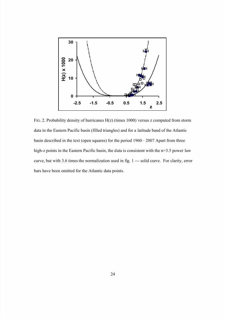
FIG. 2. Probability density of hurricanes H(z) (times 1000) versus z computed from storm
data in the Eastern Pacific basin (filled triangles) and for a latitude band of the Atlantic
basin described in the text (open squares) for the period 1960 – 2007 Apart from three
high-z points in the Eastern Pacific basin, the data is consistent with the n=3.5 power law
curve, but with 3.6 times the normalization used in fig. 1 --- solid curve. For clarity, error
bars have been omitted for the Atlantic data points.
FIG. 3 Number of storms predicted per month of the year during the period 1960 -- 2007
versus numbers actually observed for the combined Atlantic and Eastern Pacific basins.
The model predictions (continuous curve) have been normalized to the data to match the
total area.

7/29/2019 A Universal Hurricane Frequency Function
http://slidepdf.com/reader/full/a-universal-hurricane-frequency-function 22/29
22
FIG. 4 Number of storms predicted per month of the year during the period 1960 -- 2007
versus numbers actually observed for the North Asia basin (filled circles) and the Asian
Southern Hemisphere (open triangles). The model predictions (continuous curve) have
been normalized to the data to match the total area.
FIG. 5 Number of storms predicted per year during the period 1960 -- 2007 versus
numbers actually observed for the North Asia basin (open triangles), and the nearly flat
trend line fit to the data. The model predictions (continuous curve) have been normalized
to the data to match the total area.
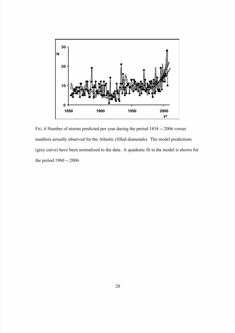
FIG. 6 Number of storms predicted per year during the period 1854 -- 2007 versus
numbers actually observed for the Atlantic (filled diamonds). The model predictions
(grey curve) have been normalized to the data. A quadratic fit to the model is shown for
the period 1960 -- 2007.
FIG. 7 Observed percentage increase in numbers of storms versus the predicted
percentage increase during the two halves of the 48 year interval 1960 -- 2007. Each data
point groups together all cells across the globe having a predicted increase falling in
decadal intervals 0 to 10%, 10 to 20%, ... The data should be consistent with a line
through the origin having unit slope shown dotted, whereas the best fit line has a slightly
larger slope.

7/29/2019 A Universal Hurricane Frequency Function
http://slidepdf.com/reader/full/a-universal-hurricane-frequency-function 23/29
23
0
5
10
15
-2.5 -1.5 -0.5 0.5 1.5 2.5z
H ( z ) x 1 0 0 0
FIG. 1. Probability density of hurricanes H(z) (times 1000) computed from storm data in
the Asian Pacific basin for the period 1960 – 2007 shown as a function of the variable z
defined in terms of the sea surface temperature T and the latitude according to
||sin)( 2/1
0 T T z with T0=25.50C, and with Southern Hemisphere data artificially
displayed as having negative z-values. H(z) represents the probability of having a storm
per month for a given z-interval. The size of the horizontal and vertical error bars is
discussed in the text. The data is consistent with the n=3.5 power law curve.
7/29/2019 A Universal Hurricane Frequency Function
http://slidepdf.com/reader/full/a-universal-hurricane-frequency-function 24/29
24
0
10
20
30
-2.5 -1.5 -0.5 0.5 1.5 2.5z
H ( z ) x 1 0 0 0
FIG. 2. Probability density of hurricanes H(z) (times 1000) versus z computed from storm
data in the Eastern Pacific basin (filled triangles) and for a latitude band of the Atlantic
basin described in the text (open squares) for the period 1960 – 2007 Apart from three
high-z points in the Eastern Pacific basin, the data is consistent with the n=3.5 power law
curve, but with 3.6 times the normalization used in fig. 1 --- solid curve. For clarity, error
bars have been omitted for the Atlantic data points.

7/29/2019 A Universal Hurricane Frequency Function
http://slidepdf.com/reader/full/a-universal-hurricane-frequency-function 25/29
25
0
100
200
300
400
1 2 3 4 5 6 7 8 9 10 11 12
month
N
FIG. 3 Number of storms predicted per month of the year during the period 1960 -- 2007
versus numbers actually observed for the combined Atlantic and Eastern Pacific basins.
The model predictions (continuous curve) have been smoothed, and have been
normalized to the data.}

7/29/2019 A Universal Hurricane Frequency Function
http://slidepdf.com/reader/full/a-universal-hurricane-frequency-function 26/29
26
0
100
200
300
1 2 3 4 5 6 7 8 9 10 11 12
month
N
FIG. 4 Number of storms predicted per month of the year during the period 1960 -- 2006
versus numbers actually observed for the North Asia basin (filled circles) and the Asian
Southern Hemisphere (open triangles). The model predictions (continuous curve) have
been smoothed, and have been normalized to the data.}

7/29/2019 A Universal Hurricane Frequency Function
http://slidepdf.com/reader/full/a-universal-hurricane-frequency-function 27/29
27
0
20
40
60
1960 1970 1980 1990 2000 2010yr
N
FIG. 5 Number of storms predicted per year during the period 1960 -- 2006 versus
numbers actually observed for the North Asia basin (open triangles), and the nearly flat
trend line fit to the data. The model predictions (dashed continuous curve) have been
smoothed, and have been normalized to the data.
7/29/2019 A Universal Hurricane Frequency Function
http://slidepdf.com/reader/full/a-universal-hurricane-frequency-function 28/29
28
0
10
20
30
1850 1900 1950 2000
yr
N
FIG. 6 Number of storms predicted per year during the period 1854 -- 2006 versus
numbers actually observed for the Atlantic (filled diamonds). The model predictions
(grey curve) have been normalized to the data. A quadratic fit to the model is shown for
the period 1960 -- 2006.

7/29/2019 A Universal Hurricane Frequency Function
http://slidepdf.com/reader/full/a-universal-hurricane-frequency-function 29/29
0
50
100
150
200
250
300
0 50 100% incr pred
% i n
c r e a s e o b s
FIG. 7 Observed percentage increase in numbers of storms versus the predicted
percentage increase during the two halves of the 47 year interval 1960 -- 2006. Each data
point groups together all cells across the globe having a predicted increase falling in
decadal intervals 0 to 10%, 10 to 20%, ... The data should be consistent with a line
through the origin having unit slope shown dotted, whereas the best fit line has a slightly
larger slope.