UCLARecent Work

TitleA Unifying Theory of Value Based Management

Permalinkhttps://escholarship.org/uc/item/0xw5m9mz

AuthorsWeaver, Samuel C.Weston, J. Fred

Publication Date2003-11-27

eScholarship.org Powered by the California Digital LibraryUniversity of California

A Unifying Theory of Value Based Management

Samuel C. Weaver College of Business and Economics

Lehigh University scw0@lehigh.edu

J. Fred Weston The Anderson School at UCLA

University of California, Los Angeles jweston@anderson.ucla.edu

November 27, 2002 We benefited from the comments of James S. Wallace at the Meetings of the Financial Management Association, October 2002. Our thanks to Juan A. Siu for his assistance.

ABSTRACT: A Unifying Theory of Value Based Management

We identify four alternative performance metrics used in value based

management (VBM). (1) Basic is an intrinsic value analysis (IVA), the discounted cash

flow (DCF) methodology. (2) We show that this framework will be consistent with

returns to shareholder (RTS, capital gains plus dividends) measured over appropriate time

horizons. (3) Economic profit (EP) [also called economic value added (EVA®)] takes

from the DCF free cash flow valuation, net operating profits after taxes (NOPAT),

divided by invested capital to obtain the return on operating invested capital (ROIC) less

a cost of capital estimate (k); the difference multiplied times operating capital. (4) The

relationship between the market value of the firm’s financial instruments and the book

value of the firm’s operating assets can be expressed equivalently as market value added

(MVA), the q ratio, and the market-to-book ratio.

We test the relationships of alternative financial accounting performance metrics

versus market metrics on a historical basis as well as on a prospective basis. We find that

the alternative financial performance metrics – discounted cash flow valuation, returns to

shareholders, economic profit, the market to book ratio [equivalently, the q ratio and

market value added (MVA)] are highly correlated. We also find that standard financial

ratio analysis as expressed in the DuPont formulation are also significantly related to

market performance metrics and in the implementation of VBM.

In implementation, each approach to value based management (VBM) starts with

strategic planning processes, ties performance to incentive compensation, requires top

management involvement, as well as information and training programs for employees.

The four approaches to VBM also take into account other stakeholders (employees,

consumers, community). VBM must also evaluate changing economic, cultural, and

political environments. The strategic planning process analyzes long term trends,

cyclical economic changes, competitive forces, and effective development of managerial

capabilities and other resources. Our clinical analysis centers on Hershey Foods

Corporation.

2

A Unifying Theory of Value Based Management

The literature on value based management contains many unsettled issues,

particularly alternative performance measurement theories (Martin and Petty, 2000;

Rappaport, 1998; Stewart, 1991; Young and O’Byrne, 2001; Copeland et al, 2000).

Divergent views are also reflected in the extensive bibliography developed by Korajczyk

(2001).

This paper seeks to develop a unifying framework for understanding value based

management (VBM). Its central elements are portrayed in Figure 1. The overview of

relationships presented demonstrates that VBM is a continuous process. It begins with

strategic planning to achieve competitive advantages which produce superior growth in

economic profits and returns to shareholders. Strategic planning guides the firm’s choice

of a product-market scope and its resource requirements. The economic nature of the

industry or industries in which the firm operates determines the patterns of its financial

statements reflected in traditional financial ratio analysis. Based on a business economic

analysis of the industry and the firm’s competitive position, projections of financial

relationships provide a basis for valuation estimates. Since these are subject to error and

change, further analysis based on identification of the key drivers of value are made.

This facilitates study of the impact of operating performance on the value driver levels

and the resulting valuations. Intrinsic value estimates are related to alternative

performance measurements. Compensation systems should be linked to performance

metrics. Periodic reviews lead to strategy revisions as well as to changes in policies and

operations. Repeated iterations of the process shown in Figure 1 are made.

3

Multiple methods of performance measurements are widely used in the literature.

They are: (1) discounted cash flow (DCF) valuation using intrinsic value analysis (IVA);

(2) returns to shareholders (RTS); (3) economic profit (EP) or economic value added

(EVA®), measured on an average and on an incremental basis; (4) the relationship

between the market value of the firm’s financial instruments and the book value of the

firm’s operating assets. This relationship has been variously called market value added

(MVA), the q ratio, and the market-to-book ratio. All measurements should be based on

projections or expectations.

This paper will compare the strengths and limitations of each performance

measure. We use data for Hershey Foods to quantify the comparisons and relationships.

In the third edition of Copeland et al (2000), data for Hershey was also used; we extend

their study. Martin and Petty (2000) also made illustrative calculations for different

companies for different measures; by using one company we can more directly compare

alternative performance measures. Ittner and Larcker (1998, 2001) provide useful

reviews of the current state of the literature. Our aim is to lay a foundation for additional

company samples or generalized research. We discuss each of the four measures in turn,

followed by comparisons between them as a basis for our conclusions.

Valuation Measurements

The uses of the four valuation measurements are first reviewed.

Intrinsic Value Analysis

We make discounted cash flow (DCF) intrinsic value estimates of Hershey Foods

for the seven year period 1994-2000. This period reflects strategy changes which

4

resulted in major restructuring activities by Hershey. Our discounted cash flow analysis

reflects the fundamental strategy shifts of Hershey. The pasta and restaurant business

were unrelated to Hershey’s core chocolate business so were divested. Hershey also

divested some foreign operations that it had not been managing effectively. It formulated

some strategic objectives: (1) Broaden the scope of its chocolate products. (2) Further

develop its lines of non-chocolate candy, chewing gum, and other confectionery products.

(3) Make entries into high growth segments of other related snack products.

Divestitures of its restaurant and pasta businesses improved Hershey’s gross

margin. Hershey also sold off its chocolate operations in Germany and Italy to an

affiliate of Huhtamäki Oy (based in Finland). Concurrently, it acquired Huhtamäki’s

Leaf North America (Leaf) confectionery operations. In addition, the parties entered into

a trademark and technology license agreement under which Hershey will manufacture

and/or market and distribute in North, Central and South America Huhtamäki's strong

confectionery brands including Good & Plenty, Heath, Jolly Rancher, Milk Duds, Payday

and Whoppers.

In December 2000, Hershey completed the purchase of the breath freshener mints

and gum businesses of Nabisco, Inc. The businesses included Ice Breakers and Breath

Savers Cool Blasts intense mints, Breath Savers mints, and Ice Breakers, Carefree,

Stick*Free, Bubble Yum and Fruit Stripe gums.

As a result of this restructuring, Hershey transformed itself into solely a chocolate

and confectionery company while enhancing its domestic market share to 26.8%

compared to Mars at 17.0% domestic market share. These strategy changes took Hershey

out of two unrelated businesses (pasta and restaurants). Hershey moved from chocolate

5

into broader candy markets. This major strategy shift improved profit margins. It also

initiated some penetration into the broader snack market which grows at a 6% rate per

annum compared to a 2% growth rate for the food industry as a whole.

These strategy changes are reflected in the valuation calculations presented in

Table 1. The methodology employed is the widely used discounted cash flow (DCF)

analysis which could be expressed in spreadsheets or in equivalent formulas (see

Copeland et al, 2000; Cornell, 2001; Rappaport, 1998). The formula employed in Table

1 uses two stages. Stage 1 is a period of competitive advantage during which the firm has

favorable growth and profitability rates. Stage 2 is the terminal period beginning at the

end of Stage 1 and running to infinity with lower growth rates and profitability. A

formula which utilizes the value drivers shown in Panel A of Table 1 is:

nscc

ocfcwcccccn

s

n

s

osfswssss

nscc

ocfcwcccccn

s

n

tt

s

ts

osfswssss

kgkIIIdTmggR

hh

kIIIdTmR

kgkIIIdTmggR

kgIIIdTmRV

)1)((])1()[1()1(

1)1(1

])1([

)1)((])1()[1()1(

)1()1(])1([

0

1

0

100

+−−−−+−++

+

−++

−−−+−=

+−−−−+−++

+

++−−−+−= ∑

=

The symbols in the formula are defined in Table 1. A numerical example of the use of

the formula using 2000 as the base year is:

V0 = 4516.4 [0.15(1-0.388)+0.03-0.002-0.028-0.001][1/(1+0.095)][(0.977210-1)/-0.0228]

+ 4220.976 [(1+0.07)10][1+0.045][0.146(1-0.388)+0.029-0.002-0.029-0.001]/[(0.095-0.045) (1+0.095)10]

= 4516.4 (0.0908) (0.9132) (9.0327)+4220.976 (1.9672) (1.045) (0.0864) [(20) (0.4035)]

= 3382.7 + 6046.9

= $9,430 million

6

The calculations reflect both the historical data and projections. Since the number

of years of competitive advantage shown in the base year 2000 column is 10 years, the

calculations reflect yearly projections for 2001 to 2010 and for the terminal stage. To

make the projections for the 17 value drivers, we drew on company presentations,

analysts’ reports, and our own studies of the economics of the industry and firm. The

measurement procedures reflect standard DCF methodology, widely used and described

in the valuation literature.

The behavior of the value drivers in Table 1 reflects the results of the operating

and financial restructuring by Hershey during the 1990s. Hershey concentrated its

business on its core competency of producing, marketing, and distributing chocolate and

confectionery products. Management was able to improve growth, margins, and the

period of competitive advantage while reducing investment needs (both working and

fixed capital) and the cost of capital. Steady improvement lead to an ever-increasing

intrinsic value per share.

As illustrated by the formulas, calculations are made for the two stages as shown

in Panel B, Lines 1 and 2 to obtain the enterprise operating value presented in Line 3.

Excess cash in the form of marketable securities is added in Line 4 to obtain the

enterprise value shown in Line 5. Deducting total interest bearing debt, we obtain the

equity value in Line 7. Line 8 presents the yearend number of shares outstanding for

Hershey for each year. Note, the number of shares declines over the years reflecting the

share repurchase program employed. In Line 9, the intrinsic value per share results for

Hershey are presented. By intrinsic value per share we mean a financial economist’s

7

effort to make an objective estimate of the economic value per share based on the

underlying determinants reflected in the value drivers.

In Lines 10 and 11 of Table 1, we compare our estimates of intrinsic value with

the actual closing price per share for Hershey over the 1994-2000 period. Martin and

Petty (2000, pp. 184-195) summarized the results of other studies comparing valuation

estimates to actual market values. The best performance appears to be the Kaplan and

Ruback (1995) study. Approximately 60% of their DCF forecasts were within ±15% of

actual transaction values. With one exception, all of our estimates were within that

range. Our estimates were based on steady improvements of the value drivers over the

restructuring activity of Hershey during the 1990s. The actual market prices anticipated

future improvements in value drivers more fully than our projections. The market reacted

much more severely to the failures of the new inventory and shipping system installed by

Hershey in 1999. Because of the glitches, Hershey was unable to ship products during

the critical August to October sales opportunities associated with Back-to-School and

Halloween. The market appeared to overact to some temporary bad news.

A major strength of the DCF models is that they seek to identify the underlying

determinants of value. Since the expectations or projections inherently are subject to

errors, the framework can be used as a valuable management planning and control

system. An ongoing monitoring of expectations compared with changing estimates of the

value drivers can be used in an information flow system. Policies and decisions can be

revised in a feedback process to improve performance. The DCF estimates of intrinsic

value can be used as a part of strategic planning processes to estimate the valuation

consequences of alternative strategic plans.

8

Table 1A presents a spreadsheet valuation consistent with the parameters of Table

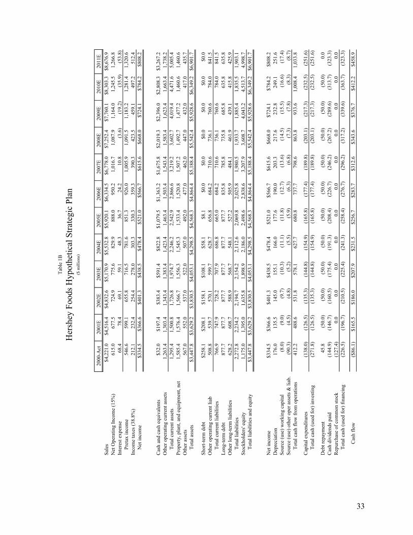
1. Table 1B provides an underlying strategic financial plan supportive of the

expectations resulting in the $60.85 per share valuation.

Returns to Shareholders

Returns to shareholders (RTS) are measured by annual capital gains plus dividend

yields. The logic of this performance metric is that it calculates the economic income to

investors for specified time periods. In Table 2 we make these calculations for Hershey

based on the yearend closing prices, shares outstanding, and dividend yield for the years

1980-2000. Because of stock market fluctuations, the results behave erratically. Two

methods are employed to deal with this instability.

One is to calculate averages over longer time periods. In Table 3 we calculate the

unweighted arithmetic average annual returns for 5- and 10-year time segments. We also

calculate the compounded annual returns to shareholders using the endpoints of each time

segment. We obtained similar results. The returns to shareholders of Hershey for the

decade of the 80s were robust. The decline in the 1991-1995 segment stimulated the

restructuring activities. Improvement was achieved during the following five years. For

the entire 20 years, the returns were about 22% per annum. When returns to shareholders

over long time periods are measured for industry segments, some economic meaning to

the results can be inferred. Returns over long periods represent what the market required

based on the risk and economic characteristics of the industry. Brealey and Myers (2000,

pp. 548-549) discuss how industry returns may be used to calculate the required return on

equity for the railroad industry, the oil industry, and for industry segments within firms.

9

The most meaningful use of returns to shareholders involves comparisons with

benchmarks. Table 4 compares the RTS measures for Hershey against the S&P500 and

the Value Line food processing index for the years 1992-2001. For the entire time

period, the RTS for Hershey shareholders was slightly above the S&P500. Benchmarked

against the food processing period, the RTS for Hershey shareholders was about the

same. Thus for the 1990s, the Hershey RTS was somewhat better than a broad index and

about the same in relation to the food processing index. The beta risk measures of the

food processing industry are similar to those of the chocolate and confectionary product

industry.

Individual year results are not dependable guides because of market volatility.

Groups of years can be selected to provide valuable information on firm performance and

economic processes. Table 5 shows RTS measure comparisons for periods ranging from

1 year to 10 years. For the longer periods, the results approximate average performance

in relation to benchmark indexes.

The use of the RTS measure permits a reasonably firm conclusion. Hershey’s

performance was comparable to the broader industry segment of which it is a part. It was

superior to the broader S&P 500 index. It would be useful to make a similar comparison

with four or five firms with products more closely comparable to Hershey’s. However,

there are no other major public chocolate and confectionary companies in the U.S. The

RTS measure is a useful indicator of performance. It can readily be applied by using

appropriate benchmarks, groups of firms, or indexes. As a performance metric, it

compares the economic returns to investors in a firm relative to alternative benchmark

10

investments. Hershey competes for the consumer’s dollar; it also competes for the

investor’s dollar.

Economic Profit Measures

Economic profit has been distinguished from accounting measures of net income

by deducting a charge for the use of capital invested. For example, suppose the

accounting net income is $120. If the firm has a book total investment of $1000

appropriately measured and a cost of capital of 10%, the deduction would be $100. The

net $20 would represent economic profit or residual income. This concept was applied

by Donaldson Brown, the senior officer of General Motors, in the 1920s as a guide to

allocating resources among the multiple divisions. It also began to be applied by General

Electric in the 1950s. The consulting firm, Stern Stewart, has employed the concept in a

measure called economic value added whose abbreviation EVA® has been copyrighted.

In applying the concept, Stern Stewart makes adjustments to NOPAT which also affect

the measurement of the invested capital base. Adjustments to NOPAT seek to capitalize

expenses such as R&D and advertising over the estimated lives during which they

contribute to revenues. The exact calculation of the popularized Economic Value

Added is an unsettled issue. A recent survey of 29 EVA users revealed that all 29

calculated NOPAT and Invested Capital in slightly different ways (Weaver 2001). We

have chosen a standard approach that excludes non-US GAAP adjustments such as

capitalizing advertising and R&D.

In Table 6, the measure of economic profit is calculated for Hershey for the years

1981-2000. First, NOPAT (Line 3) is calculated as before and excludes one-time events

11

such as gains or losses from divestitures, restructuring charges, etc. as well as all interest

income or expense. Next the invested capital (IC, Line 7) is calculated as the sum of

operating working capital, net property plant and equipment, and other assets net. Said

differently, invested capital represents total assets less non-interest bearing liabilities or

simply the book value of equity plus all interest bearing debt. The average of the

beginning and ending invested capital figures are used in subsequent calculations. The

return on average invested capital (ROIC, Line 9) is defined as the ratio of NOPAT to

average invested capital. We use an average in the denominator since NOPAT is

received throughout the year.

The WACC is specified in Line 10 and estimated to have declined over this

twenty year period. The difference between ROIC and WACC is multiplied times the

average invested capital in Line 8 to obtain the average economic profit in Line 12.

While average economic profit may be a valuable tool for performance monitoring, we

also calculate economic profit based on the beginning balance of invested capital. This

measure relates directly to the valuation using economic profit. The measures track each

other very closely and demonstrate that Hershey’s economic profit was moderate until

after the restructuring activities during the 1990’s. For sensitivity analysis, alternative

costs estimates can be employed.

The Properties of Economic Profits (EP)

In his book on EVA® or EP, Stewart (1991) states that “MVA marches in lockstep

with EVA, thus confirming the usefulness of EVA as a measure of corporate

12

performance” (p. 209). He defines market value added (MVA) as the excess of the

market value of the firm (V) over its book capital.

The nature of the relationship between EP and MVA is facilitated by a simple

example in which:

r = return on capital (ROIC) = 12% k = cost of capital (WACC) = 10% Co = capital investment = $1,000 This firm was created by a capital investment of $1000, so for this example the

investment also represents the total capital of the firm. The net present value (NPV) is

calculated by subtracting the investment from the gross present value (GPV):

200$1000200,1000,110.0

)000,1(12.0Capitalor Outlay Investment

=−=−=−=

−=

oo C

krCGPVNPV

EP or EVA® is defined as before and calculated as:

EP or EVA = (r – k)C0 = (0.12 – 0.10) 1,000 = $20

NPV is the discounted value of EVA® ($20/0.10) which equals $200. Grinblatt and

Titman (2002) prove the same result for the finite period case (pp. 341-342). In both the

finite and infinite period examples, certainty is implicit. The value of the firm (V) is the

book capital of $1000 plus the NPV of $200 which total $1200. Recall that MVA is (V –

Co) which is the NPV of $200 ($1200 - $1000). Thus, in application, market value added

(MVA) reflects expectations of future cash flows and discount rates.

Table 7 prepares a valuation of Hershey Foods using discounted economic profit

instead of discounted cash flows. The model is similar to the illustrations of table 1 or

the underlying model of table 1a, in that there is an explicit 10-year period. However,

this approach does not capitalize year 11’s cash flow as a perpetual residual value. This

13

model captures the assumptions of the residual period and extends the financial strategic

plan into the future for 250 years. Table 7 shows the first 10 years as well as years 50,

100, 150, 200, and 250. The resulting value is consistent with the enterprise operating

value presented before at $9,430 million.

Since economic profit (regardless of how it is named) is equivalent to an NPV

measure, it is an equivalently sound guide to investment decision making as is traditional

discounted cash flow analysis. Both economic profit and traditional intrinsic value (or

strategic financial modeling) can be used to measure the effectiveness of investment

decisions at the level of the firm or to segments such as divisions or plants.

Tests of EP Measures

Economic profit or economic value added has been widely evaluated and tested.

Rappaport (1998) argues that even after adjustments for multi-year effects of R&D, as

well as advertising and reversing cumulative goodwill amortization, the “shortcomings of

EVA” remain those of “a historical, sunk-cost measure” (p. 226). Young and O’Byrne

(YO) (2001) argue that with appropriate accounting adjustments such as sinking-fund

depreciation which makes ROIC equal to the economic return, the criticisms of EVA® no

longer hold. They also question the empirical study of Biddle, Bowen, and Wallace

(1997) which found that earnings data have more explanatory power for changes in stock

prices than EVA® (YO, pp. 263-267). Wallace (1997) studied the internal incentive

effects of adopting performance measures based on residual income. He found that firms

do get what they measure and reward. Managers make decisions consistent with the

performance measures adopted. Hogan and Lewis (2000) studied 51 firms adopting

14

economic profit plans. They have a control group of firms based on industry, size, and

pre-event performance. They found significant performance improvements for firms

which adopt economic profit plans. They also found similar performance improvements

for control firms. They conclude that economic profit plans are no better than alternative

plans in improving shareholders’ wealth.

While the approaches to value based management differ among theorists and

practitioners, consulting firms use a wide range of approaches. Their analyses include

strategy, financial ratio analysis, and nonfinancial criteria. Their accumulated experience

enables both the new and the traditional plans to make significant contributions to the

improvement of firm performance.

Market Valuation Ratios

Other studies of performance, particularly academic research studies, have a

measure of market value in the numerator. The q (or Tobin’s q) ratio has been widely

used to analyze the sources of differential firm efficiency related to variables such as

diversification, percentage of equity ownership by top management, etc. In theory, the q

ratio is defined as the market values of equity and debt divided by the current

replacement value of assets. In practice, the denominator is difficult to calculate. In their

early use of the q ratio at the firm level, Lindenberg and Ross (LR) (1981), arbitrarily

select a beginning date on which the replacement costs of fixed assets and inventories are

assumed to be their book values. For each subsequent year, the previous year estimate is

adjusted for general price level changes and for technological changes plus the increase

in investments less deductions for depreciation. Subsequent refinements in the LR

15

estimate were made by Chung and Pruitt (1994), Howe and Vogt (1996), Lewellen and

Badrinath (1997), and Lee and Tompkins (1999).

Whited (2001) measures Tobin’s q as the ratio of the market value of assets

divided by the book value of assets, “following the literature on corporate

diversification.” (p. 1670) The market value of assets is obtained “by adding to the book

value of assets the market value of common equity and subtracting the book value of

common equity and balance-sheet deferred taxes” (p.1671). This is equivalent to adding

to the book value of assets the difference between the market and book value of equity.

The denominator would be equivalent to the book values of equity plus debt. Whited

observes that constructing q using the algorithms of Lewellen and Badrinath in estimating

the replacement costs of assets would have reduced the number of observations without

significant change in the qualitative results (p. 1670, fn 2).

Whited replicates the results of the previous literature on corporate

diversification. When Whited employs measurement error consistent estimators, the

earlier findings no longer hold. We use the Whited definition of the q ratio in Table 8

since it is highly correlated with the other measures of q and does not require the complex

estimates of the current replacement costs of investments.

Accordingly, in Table 8, the q ratio as measured by Whited and the M/B ratio are

calculated. The data were obtained from the Hershey financial statements for 1980-2000.

Generally over the 20 year period both ratios moved upward.

The explanation for the difference is the share repurchase program of Hershey

during this period. Evidence of the magnitude of the share repurchase program is

provided by the steady decline in the number of Hershey common shares outstanding

16

from 180.4 million in 1991 to 136.3 million by 2000. When shares are repurchased, the

book based equity account is reduced by the market value of the shares repurchased.

Since 1993, when Hershey first began share repurchases, book equity was artificially

reduced by a multiple of the reduction in the number of shares outstanding. Hence, share

repurchase programs in practice inflate both the q ratio and the M/B ratio.

Relationships Between Performance Measures

At this stage, we have four valuation approaches: (1) intrinsic value, (2) returns

to shareholders, (3) economic profit, and (4) the market value added measures.

Approaches (2) and (4) directly include market or stock price information whereas the

first and third approaches are driven from company information contained within its

financial strategic plan.

Historical Relationships

Table 9A presents a correlation matrix for market valuation measures. For

Hershey Foods over the period 1983 through 2000, these metrics were all highly related

except for return to shareholders. For example, the market value of equity (MV-EQ) and

Market Value Added (MVA) had a 0.9910 R-squared, but MV-EQ compared to RTS

(return to shareholders) had an R-squared of only 0.0001.

In Table 9B, we present regression analysis to explain the movements in

operating metrics and measures of market valuation (Market Value Added, the Q-Ratio,

and Stock Price). The results of Table 9B support the following conclusions:

17

1. Regardless which market metric is used, traditional metrics such as

EBITDA, Operating Profit After Tax (OPAT), and a simple NOPAT

performed as well or better than Free Cash Flow and simple Economic

Profit. Although not reported, the simple NOPAT and EP performed as

well or better than their more sophisticated versions.

2. Return on Equity using INEX (net income excluding special items and

extraordinary items) continued to be the most significant return metric

followed closely by OPAT Return on Capital. The simple calculation of

ROIC had t-stats that did not meet the significance test, and the more

sophisticated version was significant in two of the three cases but with a

negative X-coefficient.

While the analysis above provides interesting insights for Hershey Foods, it is limited in

scope due to its historical nature and its limited 18 observations.

Relationships from the Strategic Plan

The first section of this paper developed the valuation based not in history, but in

fundamental valuation driven by a projected (and extrapolated) strategic financial plan

(Table 1B). Given this strategic financial plan (SFP), we demonstrated the equivalence

of intrinsic valuation (equation or spreadsheet) with the economic profit (or EVA®)

approaches in measuring the value of the corporation. This value is not a function of how

we measure its results; rather it is a function of the strategies that the firm employs and

the successful realization/implementation of those strategies.

18

In application, operational performance and all the performance measures can

usefully be buttressed by financial ratio analysis. Table 10 presents a compact financial

ratio analysis in the form of the traditional DuPont system. It depicts the projected one

year performance for Hershey Foods Corporation to a more detailed level than the

condensed pro-forma financial statements. The elements of cost of goods sold are

identified. Targets for R&D, marketing, and administration are set. Taxes are managed.

Working capital elements are tightly managed. Fixed assets are acquired based on net

present value principles. These elements are structured into the relationship between

OPAT and total assets. The return on assets (ROA) is depicted as a relationship between

revenues and the effective utilization of operating total assets. The analysis is extended

to include the impact of operating leverage and results in Operating Return on Capital (or

OROC).

Table 10 provides a basis for a control system to monitor and assure that the value

drivers inherent in the valuation are established, communicated, and targeted. An effort

is made to continuously improve OROC by the use of multiple performance metrics with

targets for both the long and short term. Responsibility is assigned both on a primary and

secondary basis.

Each of the performance measures has something to contribute. Each also has

limitations. Our data for Hershey show that each provides information useful for

increasing shareholder value. While some accounting measures are useful vehicles since

they underlie the intrinsic valuation of the firm, the ultimate tests are market based. The

market value and intrinsic value changes are the ultimate reference guides. They are

logically related to the other key inputs of OROC, economic market metrics, and returns

19

to shareholders. Clearly, the use of one measure alone when multiple measures can be

readily calculated is unnecessarily self limiting. A combination of performance measures

can provide useful information for planning and control systems. Multiple measures

provide a more solid basis for the development of incentive compensation programs

discussed below.

It is clear that each performance measure provides useful information, but also

has limitations. The question might be posed, “since none of the measures is perfect

what would you recommend as the performance metric of choice?” Our answer is to

employ a multiple of performance measures to obtain a more complete and reliable

assessment of performance. This is particularly important when performance measures

are used in incentive programs discussed next.

Incentive Compensation

Performance metrics are interrelated with incentive compensation. Measures of

performance achievement provide a basis for incentive compensation plans. Sound

incentive compensation programs stimulate superior performance. Some general

principles are widely accepted. Hall and Liebman (1997) developed data for the years

1980 to 1994 using Compustat, corporate proxies, plus stock price and stock return

information from CRSP. They reject the common view that there is essentially no

correlation between firm performance and CEO pay. The older view resulted from the

Jensen and Murphy (1990) finding that CEO wealth increases by only $3.25 for each

$1,000 increase in firm value, and other findings that the elasticity of CEO salary and

bonus with respect to a firm’s market value is 0.1. When the value of stock and stock

20

option holdings are taken into account, the median elasticity of CEO compensation with

respect to firm value rises to 3.9 which is 30 times larger than previous estimates. They

find that CEO wealth changes substantially with changes in firm value. They find a

difference of about $4 million in compensation for a moderately above average

performance relative to a moderately below average performance. The difference rises to

more than $9 million for 90th percentile performance versus 10th percentile stock price

performance. The Jensen and Murphy data was for 1969-83 before the rise and use of

stock options. They find that while salary and bonus is relatively insensitive to changes

in firm performance, it rapidly doubled during the 15 year period.

The level of CEO compensation increased substantially between 1980 and 1994.

The rise in the use of stock option grants was associated with sharply rising stock prices.

Direct compensation including the value of annual stock option grants increased by 136%

(median) and 209% (mean) in real terms. The mean elasticity of CEO compensation with

respect to firm market value increased from 1.2 to 3.9 between 1980 and 1994.

They find that these large increases in CEO pay during the 15 year period are

small relative to the market value of the firm and the number of employees. They note

that if annual CEO direct compensation were reduced to 1980 levels with the annual

savings returned to shareholders, their returns would increase by only 0.04 percentage

points. If the savings were distributed to workers, the median per worker gain would be

$63.

Hall and Liebman observe that a defect of CEO compensation schemes is that

“relative pay” is not a substantial component of CEO compensation. They find that

changes in direct pay, which have a relative pay component, are small relative to changes

21

in the value of stock and stock option holdings which have no relative pay component.

This leads them to suggest that the use of options with an exercise price that adjusts for

market or industry index would increase relative pay in CEO contracts.

Others have also endorsed the use of stock option indexed programs, despite

adverse accounting effects. In contrast to fixed price options, the annual cost of indexed

options must be charged to current earnings. Indexed options are central to the proposals

for incentive compensation by a number of writers (see Rappaport, 1999; Rappaport and

Mauboussin, 2001). However, the use of indexed options has some costs. Meulbroek

(2001) argues that the firm-specific risks that align incentives impose costs on executives

since they can no longer fully diversify their portfolios. Financial engineering can

eliminate the systematic portion of risk to executives but cannot eliminate the firm-

specific exposures. Executives will value their equity-based compensation at less than its

market value. Thus a firm faces a trade off between incentive alignment and the cost of

paying executives with instruments that otherwise could be sold at a higher price.

Up to this point the discussions have been limited to incentive compensation for

top level executives. For executives of operating divisions or segments, stock price data

are not available. The calculations of intrinsic shareholder value nevertheless can be

performed. Only the discount factor requires market data. This can be obtained from

estimates of the cost of capital for “pure play” companies. Beta adjustments can be made

using the standard formulas for the relationship between levered and unlevered betas.

Calculations can be made for the value and changes in value of the segment. If

performance measurement problems are severe, the possibility of a spin-off can be

considered.

22

For other critical employees and managers, contributions to enterprise value can

be estimated. A clear example is the materials in the annual reports of Ruby Tuesday, a

chain of restaurants operating in the East. Figure 2 represents communications provided

to all employees. This broad sharing of information carries positive benefits for

employee involvement. Also notable is a list of indicators that are likely to be highly

correlated with financial results: sales levels, food quality ratings, customer satisfaction

scores, employee turnover, team satisfaction scores. In addition, financial metrics are

employed. These include EPS growth targets, pretax sales margin, and return on equity.

Each of these metrics is subject to limitations and misuse. However, imperfect metrics

can still provide powerful incentives and motivations if used as guidelines and as

instruments of communication. Used with judgment and continuous monitoring such

metrics can make valuable contributions to performance.

Relationships

On conceptual and analytical criteria most writers emphasize the preeminence of

intrinsic valuation approaches using spreadsheets or formulas. Intrinsic value measures

should relate to returns to shareholders as well as to market value changes. However,

market expectations sometimes run ahead of or behind intrinsic value measurements. As

a consequence there are no perfect consistencies between intrinsic value, returns to

shareholders, and changes in market value.

Economic profit or economic value added programs have been effectively

promoted. Since they involve a return on invested capital and a discount factor, ROIC

and WACC also need to be measured. The intrinsic value measures are most sensitive to

23

estimates of sales growth and the NOI margin. In turn, the NOI margin depends on the

control of costs. The return metrics require effective management of working capital and

fixed investments which are analyzed in the DuPont chart shown in Table 10.

Thus all of the alternative measures of performance can provide useful inputs to a

program of value based management. Even measures subject to ambiguity or abuse can

provide useful inputs. They can also be used for motivation. We use the Ruby Tuesday

(RT) example because of its success in the highly competitive restaurant business.

Between 9/30/91-9/30/01, RT achieved a 19.87% annualized growth in equity values

compared to the S&P 500 of 12.41% and the restaurant index of 8.25%.

The outstanding performance of RT demonstrates that multiple measures of

performance, in addition to indicators such as measures of customer satisfaction and

effective human resource program, can reinforce financial measures. RT has been

innovative in incentive management as well. More than 55% company owned franchises

permit managers to invest their own funds, for which they receive a percentage of the

profits. In addition, RT has stock option programs that include non-executives. A

committee appointed by the board has authority to determine the officers and employees

to whom stock incentives are granted.

Thus a complete value based management system includes financial measures,

indicators of external economic and financial developments, as well as active top

management and board involvement on a continuing basis.

24

Conclusions

This unifying theory of value based management (VBM) identifies multiple

approaches. Four have been widely used in practice. One is intrinsic value analysis

(IVA) also called shareholder value added (SVA). Two is returns to shareholder (RTS).

Three is economic profit. Four is the relationship between the market value of the firm’s

financial instruments and the book value of the firm’s operating assets. This relationship

has been called market value added (MVA), the q ratio, and the market-to-book ratio.

Statistically, MVA, the q ratio, and M/B measure the same thing. Analysis of the

structure of income, costs, and investments is employed in implementing the previous

four approaches.

In application, the four approaches to VBM have a high degree of similarity.

Each embraces and utilizes the framework we present in Figure 1. The key elements

include strategic review and organizational structure related to strategy performance

measurements, incentive compensation systems related to performance measures,

implementation (involvement and support of top executives and training throughout the

organization), and continuous review and renewal. The company profiles in Martin and

Petty (2000) illustrate this generalization. The four VBM approaches are all represented.

In the success stories by proponents of the alternative approaches to VBM, the

multiple elements of applications are illustrated. For example, Briggs & Stratton (air-

cooled gasoline engines) had lagged in recognition of its changed competitive

environment, had not focused on its core competencies, and attempted to solve its

problems by automating its production processes. Capital invested to net income

increased from 300% to over 900% during the 80’s (Stern et al, 2001). At Herman Miller

25

(office furniture) losses resulted from undisciplined multiple product proliferation. The

problems involved strategy, structure, and financial control (Stern et al, 2001). Similar

stories for seven companies are told of adopters of the balanced scorecard (Kaplan and

Norton, 1996). The balanced scorecard also has multiple metrics including nonfinancial

criteria (see also Eccles et al, 2000).

Despite the similarities in methodology, each of the proponents of a particular

emphasis of VBM argues for its distinctive superiority and for defects or limitations in

the approaches of its competitors. Intrinsic value analysis (IVA) or shareholder value

added (SVA) performs a DCF valuation of cash flows over long time horizons. Changes

in value can also be measured yearly by reference to returns to shareholders (RTS) or by

market value added (MVA), the market-to-book ratio, and the q ratio. Market prices may

overstate or understate intrinsic value for periods of time.

Economic profit (EP) or economic value added (EVA®) can be criticized for

focusing on a single metric which includes an accounting return. In utilization, economic

value added includes strategy, structure, financial ratio analysis, and roadmaps to value

creation that include consideration of a wide range of stakeholders (employees,

customers, suppliers, community) (Stern et al, 2001). In practice, it would be difficult to

distinguish between the applications of the balanced scorecard versus economic value

added. Interestingly, Rappaport’s (1998) final chapter includes compilations of “the

shareholder scoreboard” based on returns to shareholders (percentage changes in capital

gains plus dividends for selected time periods). Stewart (1991) ends his book with a

scorecard entitled “Performance 1000” based on market value added (MVA).

26

In theory the four alternative approaches to VBM are somewhat different. In

practice, the implementations have similarities in methodology and coverage. They all

center on strategic financial planning and appear to make valuable contributions to

performance improvement and to value creation. The empirical evidence argues for an

eclectic approach to value based management. Intrinsic value DCF analysis, returns to

shareholders or the shareholder scoreboard, economic value added, and the market-to-

book analysis have all enhanced value. Each could contribute to effective information

planning and control processes.

The downturn beginning in 2000 emphasizes that external economic indicators

are an important part of value based management. Also indicators of performance in

relation to stakeholders such as employees and consumers are useful. If a firm does not

score well in these areas, it is not likely to score well in the effort to add to shareholder

value. With the aid of computers, multiple performance measures can be employed.

This also permits communication of financial goals and performance widely throughout

the organization. Continuous information exchange stimulates managers and informs top

executives. Value based management requires multiple performance measures with

support from top executives who interact over a wide range of managers on an informed

basis.

27

References

Biddle, Gary C., Robert M. Bowen, and James S. Wallace, 1997, “Does EVA Beat

Earnings? Evidence on Associations with Stock Returns and Firm Values,” Journal of Accounting and Economics, 24 (No. 3, December), 301-336.

Brealey, Richard A., and Stewart C. Myers, 2000, Principles of Corporate Finance, 6th Edition, Boston: Irwin/McGraw-Hill.

Chung, Kee H. and Stephen W. Pruitt, 1994, “A Simple Approximation of Tobin’s q,” Financial Management, 23 (3, Autumn), 70-74.

Copeland, Tom, 2002, “What do Practitioners Want?” Journal of Applied Finance, 12 (No. 1, Spring/Summer), 5-12.

Copeland, Tom, Tim Koller, and Jack Murrin, 2000, Valuation: Measuring and Managing the Values of Companies, 3rd ed., New York: John Wiley & Sons.

Cornell, Bradford, 2001, “Is the Response of Analysts to Information Consistent with Fundamental Valuation? The Case of Intel,” Financial Management, 30 (No. 1, Spring), 113-136.

Eccles, Robert G., Robert H. Herz, E. Mary Keegan, and David M. H. Phillips, 2001, The Value Reporting Revolution: Moving Beyond the Earnings Game, New York: John Wiley & Sons.

Grinblatt, Mark, and Sheridan Titman, 2002, Financial Markets and Corporate Strategy, 2nd edition, Boston: Irwin/McGraw-Hill.

Hall, Brian J., and Jeffrey B. Liebman, 1998, “Are CEOs Really Paid Like Bureaucrats?” Quarterly Journal of Economics, 113 (No. 3, August), 653-691.

Hogan, Chris, and Craig Lewis, 2000, “The Long-Run Performance of Firms Adopting Compensation Plans Based on Economic Profits,” Owens Graduate School of Management Working Paper, (May).

Howe, Keith M. and Stephen Vogt, 1996, “On 'q',” Financial Review, 31 (2, May), 265-286.

Ittner, Christopher D. and David F. Larcker, 1998, “Innovations in Performance Measurement: Trends and Research Implications,” Journal of Management Accounting Research, 10, 205-238.

Ittner, Christopher D. and David F. Larcker, 2001, “Assessing Empirical Research in Managerial Accounting: A Value-Based Management Perspective,” Journal of Accounting and Economics.

28

Jensen, Michael C., and Kevin J. Murphy, 1990, “Performance Pay and Top-Management Incentives,” Journal of Political Economy, 98 (No. 2, April), 225-264.

Kaplan, Robert S., and David P. Norton, 1996, The Balanced Scorecard, Boston: Harvard Business School Press.

Korajczyk, Robert A., 2001, “Papers on Value-Based Management,” October 12, <www.kellogg.nwu.edu/faculty/korajczy/htm/vbm.htm>.

Kramer, Jonathan K. and Jonathan R. Peters, 2001, “An Interindustry Analysis of Economic Value Added : as a Proxy for Market Value Added,” Journal of Applied Finance, 11 (No. 1, Fall/Winter), 41-49.

Lee, Darrell E. and James G. Tompkins, 1999, “A Modified Version of the Lewellen and

Badrinath Measure of Tobin’s Q,” Financial Management, 28 (1, Spring), 20-31.

Lewellen, Wilbur G. and S. G. Badrinath, 1997, “On the Measurement of Tobin’s q,” Journal of Financial Economics, 44 (1, April), 77-122.

Lindenberg, Eric B. and Stephen A. Ross, 1981, “Tobin's q Ratio and Industrial Organization,” Journal of Business, 54 (1, January), 1-32.

Martin, John D., and J. William Petty, 2000, Valued Based Management: The Corporate Response to the Shareholder Revolution, Boston: Harvard Business School Press.

Meulbroek, Lisa, 2001, “The Efficiency of Equity-Linked Compensation: Understanding the Full Cost of Awarding Executive Stock Options,” Financial Management, 30 (No. 2, Summer), 5-44.

Rappaport, Alfred, 1998, Creating Shareholder Value: A Guide for Managers and Investors, New York: The Free Press.

Rappaport, Alfred, 1999, “New Thinking on How to Link Executive Pay with Performance,” Harvard Business Review, 77 (No. 2, Mar-Apr), 91-101.

Rappaport, Alfred, and Michael J. Mauboussin, 2001, Expectations Investing: Reading Stock Prices for Better Returns, Boston: Harvard Business School Press.

Stern, Joel M., and John S. Shiely, with Irwin Ross, 2001, The EVA Challenge: Implementing Value-Added Change in an Organization, New York: John Wiley & Sons.

Stewart, G. Bennett, III, 1991, The Quest for Value, New York: HarperBusiness.

Wallace, James S., 1997, “Adopting Residual Income-Based Compensating Plans: Do You Get What You Pay For?” Journal of Accounting and Economics, 24 (No. 3, December), 275-300.

29

Weaver, Samuel C., 2001, “Measuring Economic Value Added : A Survey of the Practices of EVA Proponents,” Journal of Applied Finance, 11 (No. 1, Fall/Winter), 50-60.

Whited, Toni M., 2001, “Is It Inefficient Investment that Causes the Diversification

Discount?’ Journal of Finance, 56 (No. 5, October), 1667-1691.

Young, S. David, and Stephen F. O’Byrne, 2001, EVA and Value-Based Management: A Practical Guide to Implementation, New York: McGraw-Hill.

30

Figure 1

A Unifying Theory of Value Based Management (VBM)

Strategic Plans

Balance SheetsIncome Statements

Cash Flow Statements

Historical Financial

Ratios Business Economics Analysis of

Firm’s Future

Projections of Financial

Statements

Spreadsheets of Value

Driver Data for ValuationValuation

Sensitivity Analysis

Performance Measurement

1. Returns to shareholders (RTS)

2. Return on Invested Capital (ROIC)

3. Economic Profit4. Market-to-book relations

Performance Review and

Strategy Revisions

Financial Implications of

Alternative Strategies

1

2 3

4

5

67

89

10

11

Linking Compensation to

Performance Measurements

31

Table 1 Intrinsic Value Estimates, 1994-2000

(Dollar Amounts in Millions Except Per Share)

1994 1995 1996 1997 1998 1999 2000Panel A - Value Drivers

R0 = Base year revenues 3,606$ 3,691$ 3,989$ 4,302$ 4,436$ 3,971$ 4,221$

Initial Growth Stagems = Net operating income margin 13.9% 14.3% 14.4% 15.0% 15.0% 15.0% 15.0%Ts = Tax rate 45.4% 33.8% 38.3% 36.2% 24.0% 37.9% 38.8%gs = Growth rate 5.1% 5.4% 6.0% 6.6% 6.8% 6.8% 7.0%ds = Depreciation 3.0% 3.0% 3.0% 3.0% 3.0% 3.0% 3.0%

Iws = Working capital requirements 0.2% 0.2% 0.2% 0.2% 0.2% 0.2% 0.2%Ifs = Capital expenditures 3.7% 3.5% 3.4% 3.1% 2.6% 2.6% 2.8%Ios = Change in other assets, net 0.1% 1.0% 0.1% 0.1% 0.1% 0.1% 0.1%ks = Cost of capital 10.0% 9.9% 9.8% 9.5% 9.5% 9.5% 9.5%n = Number of growth years 5 6 7 9 9 9 10

Terminal stagemc = Net operating income margin 12.0% 12.2% 14.3% 14.6% 14.6% 14.6% 14.6%Tc = Tax rate 38.8% 38.8% 38.8% 38.8% 38.8% 38.8% 38.8%gc = Growth rate 4.0% 4.1% 4.2% 4.3% 4.3% 4.4% 4.5%dc = Depreciation 2.9% 2.9% 2.9% 2.9% 2.9% 2.9% 2.9%

Iwc = Working capital requirements 0.10% 0.12% 0.14% 0.15% 0.16% 0.18% 0.20%Ifc = Capital expenditures 2.4% 2.5% 2.6% 2.6% 2.7% 2.7% 2.9%Ioc = Change in other assets, net 0.1% 0.1% 0.1% 0.1% 0.1% 0.1% 0.1%Kc = Cost of capital 10.0% 9.9% 9.8% 9.5% 9.5% 9.5% 9.5%

1 + h = Calculation relationship = (1+gs)/(1+ks) 0.9555 0.9591 0.9654 0.9735 0.9753 0.9753 0.9772

Panel B - Calculating Firm Value1. Present value of initial growth stage cash flow 1,038$ 1,661$ 1,991$ 3,110$ 4,059$ 2,976$ 3,383$ 2. Present value of terminal value 3,805 3,941 5,112 6,090 6,307 5,750 6,047

3. Enterprise operating value 4,843$ 5,602$ 7,103$ 9,200$ 10,366$ 8,726$ 9,430$ 4. Add: Marketable securities - - - - - - -

5. Entity value 4,843$ 5,602$ 7,103$ 9,200$ 10,366$ 8,726$ 9,430$ 6. Less: Total interest-bearing debt 505 796 996 1,317 1,282 1,118 1,136 7. Equity value 4,338$ 4,806$ 6,107$ 7,883$ 9,084$ 7,608$ 8,294$ 8. Number of shares 173.5 154.5 152.9 142.9 143.1 138.5 136.3

9. Intrinsic value per share 25.00$ 31.11$ 39.94$ 55.16$ 63.48$ 54.93$ 60.85$

10. Actual closing price per share 24.19$ 32.50$ 43.75$ 61.94$ 62.19$ 47.44$ 64.38$ 11. Percent difcference from closing price 3.4% -4.3% -8.7% -10.9% 2.1% 15.8% -5.5%

32

Tabl

e 1A

DC

F Sp

read

shee

t Val

uatio

n of

Her

shey

($

mill

ions

)

Pane

l A -

Valu

atio

n A

ssum

ptio

ns20

01E

2002

E20

03E

2004

E20

05E

2006

E20

07E

2008

E20

09E

2010

E20

11E

Net

reve

nues

(gro

wth

rate

s)7.

0%7.

0%7.

0%7.

0%7.

0%7.

0%7.

0%7.

0%7.

0%7.

0%4.

5%Ta

x ra

te38

.8%

38.8

%38

.8%

38.8

%38

.8%

38.8

%38

.8%

38.8

%38

.8%

38.8

%38

.8%

(As a

% o

f rev

enue

s)N

OI

15.0

%15

.0%

15.0

%15

.0%

15.0

%15

.0%

15.0

%15

.0%

15.0

%15

.0%

14.6

%N

OPA

T9.

2%9.

2%9.

2%9.

2%9.

2%9.

2%9.

2%9.

2%9.

2%9.

2%8.

9%

Dep

reci

atio

n3.

0%3.

0%3.

0%3.

0%3.

0%3.

0%3.

0%3.

0%3.

0%3.

0%2.

9%

Cha

nge

in w

orki

ng c

apita

l-0

.2%

-0.2

%-0

.2%

-0.2

%-0

.2%

-0.2

%-0

.2%

-0.2

%-0

.2%

-0.2

%-0

.2%

C

apita

l exp

endi

ture

s-2

.8%

-2.8

%-2

.8%

-2.8

%-2

.8%

-2.8

%-2

.8%

-2.8

%-2

.8%

-2.8

%-2

.9%

C

hang

e in

oth

er a

sset

s net

-0.1

%-0

.1%

-0.1

%-0

.1%

-0.1

%-0

.1%

-0.1

%-0

.1%

-0.1

%-0

.1%

-0.1

%

Pane

l B -

Spre

adsh

eet D

ata

2001

E20

02E

2003

E20

04E

2005

E20

06E

2007

E20

08E

2009

E20

10E

2011

EN

et re

venu

es4,

516.

5$

4,

832.

6$

5,

170.

9$

5,

532.

9$

5,

920.

2$

6,

334.

6$

6,

778.

0$

7,

252.

5$

7,

760.

1$

8,

303.

3$

8,

677.

0$

N

OI

677.

572

4.9

775.

682

9.9

888.

095

0.2

1,01

6.70

1,

087.

87

1,16

4.02

1,

245.

50

1,26

6.84

Inco

me

taxe

s26

2.9

281.

330

0.9

322.

034

4.6

368.

739

4.5

422.

145

1.6

483.

349

1.5

NO

PAT

414.

6$

443.

6$

474.

7$

507.

9$

543.

5$

581.

5$

622.

2$

665.

8$

712.

4$

762.

2$

775.

3$

D

epre

ciat

ion

135.

514

5.0

155.

116

6.0

177.

619

0.0

203.

321

7.6

232.

824

9.1

251.

6

Cha

nge

in w

orki

ng c

apita

l(9

.0)

(9.7

)(1

0.3)

(11.

1)(1

1.8)

(12.

7)(1

3.6)

(14.

5)(1

5.5)

(16.

6)(1

7.4)

C

apita

l exp

endi

ture

s(1

26.5

)(1

35.3

)(1

44.8

)(1

54.9

)(1

65.8

)(1

77.4

)(1

89.8

)(2

03.1

)(2

17.3

)(2

32.5

)(2

51.6

)

Cha

nge

in o

ther

ass

ets n

et(4

.5)

(4.8

)(5

.2)

(5.5

)(5

.9)

(6.3

)(6

.8)

(7.3

)(7

.8)

(8.3

)(8

.7)

Free

cas

h flo

ws

410.

1$

438.

8$

469.

5$

502.

4$

537.

6$

575.

2$

615.

4$

658.

5$

704.

6$

753.

9$

749.

3$

WA

CC

9.5%

9.5%

9.5%

9.5%

9.5%

9.5%

9.5%

9.5%

9.5%

9.5%

Dis

coun

t fac

tor

0.91

32

0.

8340

0.76

17

0.

6956

0.63

52

0.

5801

0.52

98

0.

4838

0.44

18

0.

4035

Pres

ent v

alue

374.

5$

366.

0$

357.

6$

349.

4$

341.

5$

333.

7$

326.

1$

318.

6$

311.

3$

304.

2$

Pres

ent v

alue

- fr

ee c

ash

flow

3,38

2.9

$

Pres

ent v

alue

- re

sidu

al v

alue

6,04

6.9

$

R

esid

ual v

alue

=14

,985

.5$

(FC

F yr

11) /

(CO

C -

g) =

$74

9.3

/ (.0

95 -

.045

)En

terp

rise

oper

atin

g va

lue

9,42

9.8

$

33

Tabl

e 1B

Her

shey

Foo

ds H

ypot

hetic

al S

trate

gic

Plan

($ m

illio

ns)

2000

-Act

2001

E20

02E

2003

E20

04E

2005

E20

06E

2007

E20

08E

2009

E20

10E

2011

ESa

les

$4,2

21.0

$4,5

16.4

$4,8

32.6

$5,1

70.9

$5,5

32.8

$5,9

20.1

$6,3

34.5

$6,7

78.0

$7,2

52.4

$7,7

60.1

$8,3

03.3

$8,6

76.9

Net

Ope

ratin

g In

com

e (1

5%)

615.

067

7.5

724.

977

5.6

829.

988

8.0

950.

21,

016.

71,

087.

91,

164.

01,

245.

51,

266.

8In

tere

st e

xpen

se68

.478

.469

.159

.148

.336

.724

.210

.8(3

.6)

(19.

2)(3

5.9)

(53.

8)Pr

etax

inco

me

546.

659

9.1

655.

871

6.5

781.

685

1.3

926.

01,

005.

91,

091.

51,

183.

21,

281.

41,

320.

6In

com

e ta

xes (

38.8

%)

212.

123

2.4

254.

427

8.0

303.

333

0.3

359.

339

0.3

423.

545

9.1

497.

251

2.4

Net

inco

me

$334

.5$3

66.6

$401

.3$4

38.5

$478

.4$5

21.0

$566

.7$6

15.6

$668

.0$7

24.1

$784

.2$8

08.2

Cas

h an

d ca

sh e

quiv

alen

ts$3

2.0

$197

.4$3

83.4

$591

.4$8

22.8

$1,0

79.5

$1,3

63.2

$1,6

75.8

$2,0

19.3

$2,3

96.0

$2,8

08.3

$3,2

67.2

Oth

er o

pera

ting

curr

ent a

sset

s1,

263.

41,

303.

41,

343.

41,

383.

41,

423.

41,

463.

41,

503.

41,

543.

41,

583.

41,

623.

41,

663.

41,

738.

2To

tal c

urre

nt a

sset

s1,

295.

41,

500.

81,

726.

81,

974.

72,

246.

22,

542.

92,

866.

63,

219.

23,

602.

74,

019.

44,

471.

65,

005.

4Pr

oper

ty, p

lant

, and

equ

ipm

ent,

net

1,58

5.4

1,57

6.4

1,56

6.7

1,55

6.3

1,54

5.3

1,53

3.4

1,52

0.8

1,50

7.2

1,49

2.7

1,47

7.2

1,46

0.6

1,46

0.6

Oth

er a

sset

s56

7.0

552.

053

7.0

522.

050

7.0

492.

047

7.0

462.

044

7.0

432.

041

7.0

435.

7To

tal a

sset

s$3

,447

.8$3

,629

.2$3

,830

.5$4

,053

.1$4

,298

.5$4

,568

.3$4

,864

.4$5

,188

.4$5

,542

.4$5

,928

.6$6

,349

.2$6

,901

.7

Shor

t-ter

m d

ebt

$258

.1$2

08.1

$158

.1$1

08.1

$58.

1$8

.1$0

.0$0

.0$0

.0$0

.0$0

.0$0

.0O

ther

ope

ratin

g cu

rren

t lia

b50

8.8

539.

757

0.1

599.

762

8.7

656.

868

4.2

710.

673

6.1

760.

678

4.0

841.

5To

tal c

urre

nt li

abili

ties

766.

974

7.9

728.

270

7.9

686.

866

5.0

684.

271

0.6

736.

176

0.6

784.

084

1.5

Long

-term

deb

t87

7.7

877.

787

7.7

877.

787

7.7

877.

783

5.8

785.

873

5.8

685.

863

5.8

635.

8O

ther

long

-term

liab

ilitie

s62

8.2

608.

758

8.9

568.

754

8.1

527.

250

5.9

484.

146

1.9

439.

141

5.8

425.

9To

tal l

iabi

litie

s2,

272.

82,

234.

22,

194.

72,

154.

22,

112.

62,

069.

82,

025.

81,

980.

51,

933.

71,

885.

41,

835.

51,

903.

1St

ockh

olde

rs' e

quity

1,17

5.0

1,39

5.0

1,63

5.8

1,89

8.9

2,18

6.0

2,49

8.6

2,83

8.6

3,20

7.9

3,60

8.7

4,04

3.2

4,51

3.7

4,99

8.7

Tota

l lia

bilit

ies a

nd e

quity

$3,4

47.8

$3,6

29.2

$3,8

30.5

$4,0

53.1

$4,2

98.5

$4,5

68.3

$4,8

64.4

$5,1

88.4

$5,5

42.4

$5,9

28.6

$6,3

49.2

$6,9

01.7

Net

inco

me

$334

.5$3

66.6

$401

.3$4

38.5

$478

.4$5

21.0

$566

.7$6

15.6

$668

.0$7

24.1

$784

.2$8

08.2

Dep

reci

atio

n17

6.0

135.

514

5.0

155.

116

6.0

177.

619

0.0

203.

321

7.6

232.

824

9.1

251.

6So

urce

(use

) wor

king

cap

ital

(8.0

)(9

.0)

(9.7

)(1

0.3)

(11.

1)(1

1.8)

(12.

7)(1

3.6)

(14.

5)(1

5.5)

(16.

6)(1

7.4)

Sour

ce (u

se) o

ther

ope

r ass

ets &

liab

.(9

0.3)

(4.5

)(4

.8)

(5.2

)(5

.5)

(5.9

)(6

.3)

(6.8

)(7

.3)

(7.8

)(8

.3)

(8.7

)To

tal c

ash

flow

from

ope

ratio

ns41

2.2

488.

653

1.8

578.

162

7.7

680.

873

7.7

798.

686

3.8

933.

61,

008.

41,

033.

8

Cap

ital e

xpen

ditu

res

(138

.0)

(126

.5)

(135

.3)

(144

.8)

(154

.9)

(165

.8)

(177

.4)

(189

.8)

(203

.1)

(217

.3)

(232

.5)

(251

.6)

Tota

l cas

h (u

sed

for)

inve

stin

g(2

71.8

)(1

26.5

)(1

35.3

)(1

44.8

)(1

54.9

)(1

65.8

)(1

77.4

)(1

89.8

)(2

03.1

)(2

17.3

)(2

32.5

)(2

51.6

)

Deb

t rep

aym

ent

45.8

(50.

0)(5

0.0)

(50.

0)(5

0.0)

(50.

0)(5

0.0)

(50.

0)(5

0.0)

(50.

0)(5

0.0)

0.0

Cas

h di

vide

nds p

aid

(144

.9)

(146

.7)

(160

.5)

(175

.4)

(191

.3)

(208

.4)

(226

.7)

(246

.2)

(267

.2)

(289

.6)

(313

.7)

(323

.3)

Rep

urch

ase

of c

omm

on st

ock

(127

.4)

0.0

0.0

0.0

0.0

0.0

0.0

0.0

0.0

0.0

0.0

0.0

Tota

l cas

h (u

sed

for)

fina

ncin

g(2

26.5

)(1

96.7

)(2

10.5

)(2

25.4

)(2

41.3

)(2

58.4

)(2

76.7

)(2

96.2

)(3

17.2

)(3

39.6

)(3

63.7

)(3

23.3

)

Cas

h flo

w($

86.1

)$1

65.5

$186

.0$2

07.9

$231

.5$2

56.7

$283

.7$3

12.6

$343

.6$3

76.7

$412

.2$4

58.9

34

Table 2 Hershey, Returns to Shareholders Relationships, 1980-2000

(Adjusted for stock-splits)

1980 1981 1982 1983 1984 1985 1986 1987 1988 1989 1990

1. Closing Price $1.96 $3.00 $4.70 $5.27 $6.44 $8.58 $12.31 $12.25 $13.00 $17.94 $18.75

2. Common Shares Outstanding(millions)

169.9 188.0 188.0 188.0 188.0 188.0 180.4 180.4 180.4 180.4 180.4

3. Dividend per share $0.13 $0.15 $0.17 $0.18 $0.21 $0.24 $0.26 $0.29 $0.33 $0.37 $0.50

4. Dividend yield 7.4% 5.6% 3.9% 3.9% 3.7% 3.0% 2.4% 2.7% 2.8% 2.8%5. Capital gain 53.2% 56.6% 12.2% 22.1% 33.3% 43.4% -0.5% 6.1% 38.0% 4.5% 6. Total return to shareholders 60.6% 62.2% 16.1% 26.1% 37.0% 46.5% 1.8% 8.8% 40.8% 7.3%

1991 1992 1993 1994 1995 1996 1997 1998 1999 2000

1. Closing Price $22.19 $23.50 $24.50 $24.19 $32.50 $43.75 $61.94 $62.19 $47.44 $64.38

2. Common Shares Outstanding(millions)

180.4 180.4 175.2 173.5 154.5 152.9 142.9 143.1 138.5 136.3

3. Dividend per share $0.47 $0.52 $0.57 $0.63 $0.69 $0.76 $0.84 $0.92 $1.00 $1.08

4. Dividend yield 2.5% 2.3% 2.4% 2.6% 2.8% 2.3% 1.9% 1.5% 1.6% 2.3%5. Capital gain 18.3% 5.9% 4.3% -1.3% 34.4% 34.6% 41.6% 0.4% -23.7% 35.7% 6. Total return to shareholders 20.8% 8.2% 6.7% 1.3% 37.2% 37.0% 43.5% 1.9% -22.1% 38.0%

Data Source: Compustat

Table 3 Total Returns to Shareholders (TRS)

Period Average Annual Return

Compound Annual Return

1980-1990 30.7% 29.1%

1991-1995 13.3% 12.5%

1995-2000 19.6% 16.6%

1980-2000 24.0% 22.0%

35

Table 4 Annual RTS Measure Comparison

Year Hershey - S&P500 Hershey - Food Index

1992 3.56% -1.27%

1993 3.51% 16.73%

1994 -12.76% -17.91%

1995 3.34% 13.49%

1996 44.08% 39.92%

1997 -16.14% -28.22%

1998 2.72% 9.05%

1999 -49.53% -31.23%

2000 4.66% 3.25%

2001 44.53% 3.53%

Average 2.80% 0.73%

Table 5 RTS Measure Comparison for Selected Periods

Period Hershey - S&P500 Hershey - Food Index

1991-2001 1.87% -0.91%

1992-2001 1.68% -0.87%

1993-2001 1.46% -3.18%

1994-2001 3.86% -0.70%

1995-2001 3.94% -2.95%

1996-2001 -2.23% -9.62%

1997-2001 0.73% -5.70%

1998-2001 0.19% -10.00%

1999-2001 25.86% 3.39%

2000-2001 44.53% 3.53%

Average 8.19% -2.70%

36

Table 6Calculation of Economic Profit - Average and Beginning Invested Capital

(Dollar Amounts in Millions - Varying Cost of Capital)

1981 1982 1983 1984 1985 1986 1987 1988 1989 1990

1. NOI 167$ 179$ 205$ 220$ 245$ 271$ 294$ 266$ 310$ 351$ 2. Cash Tax Rate 42.2% 38.1% 40.7% 37.4% 35.2% 38.9% 48.7% 36.7% 39.8% 42.6%3. NOPAT 97$ 111$ 122$ 138$ 159$ 166$ 151$ 168$ 187$ 201$

4. Operating Working Capital 172$ 153$ 207$ 210$ 241$ 203$ 256$ 358$ 319$ 385$ 5. NPPE 440 540 575 643 702 793 863 736 830 952 6. Other Assets, Net 18 (1) (36) (39) (81) (26) 90 229 221 244 7. Invested Capital (IC) 630$ 692$ 746$ 814$ 862$ 970$ 1,209$ 1,323$ 1,370$ 1,581$

8. Average Invested Capital (AIC) 576$ 661$ 719$ 780$ 838$ 916$ 1,090$ 1,266$ 1,347$ 1,476$

Measures Based on Average Invested Capital

9. AROIC = NOPAT / AIC 16.8% 16.8% 16.9% 17.7% 18.9% 18.1% 13.8% 13.3% 13.9% 13.7%

10. WACC 13.0% 12.0% 12.0% 12.0% 12.0% 12.0% 12.0% 12.0% 12.0% 12.0%

11. AROIC - WACC 3.8% 4.8% 4.9% 5.7% 6.9% 6.1% 1.8% 1.3% 1.9% 1.7%

12. AEP = AIC (AROIC - WACC) 22$ 31$ 35$ 44$ 58$ 56$ 20$ 16$ 25$ 24$

Measures Based on Beginning Invested Capital

13. BROIC = NOPAT / IC(t-1) 17.6% 17.6% 18.5% 19.5% 19.2% 15.5% 13.9% 14.1% 14.7%

14. WACC 12.0% 12.0% 12.0% 12.0% 12.0% 12.0% 12.0% 12.0% 12.0%

15. BROIC - WACC 5.6% 5.6% 6.5% 7.5% 7.2% 3.5% 1.9% 2.1% 2.7%

16. AEP = IC(t-1) (BROIC - WACC) 35$ 39$ 48$ 61$ 62$ 34$ 23$ 28$ 37$

1991 1992 1993 1994 1995 1996 1997 1998 1999 2000

1. NOI 390$ 428$ 457$ 475$ 511$ 563$ 630$ 643$ 558$ 615$ 2. Cash Tax Rate 33.9% 34.2% 39.7% 45.4% 33.8% 38.3% 36.2% 24.0% 37.9% 41.8%3. NOPAT 258$ 282$ 276$ 259$ 338$ 347$ 402$ 489$ 347$ 358$

4. Operating Working Capital 382$ 409$ 443$ 500$ 496$ 509$ 527$ 722$ 807$ 787$ 5. NPPE 1,146 1,296 1,461 1,468 1,436 1,602 1,648 1,648 1,510 1,585 6. Other Assets, Net 199 141 42 (23) (54) 45 (5) (46) (101) (61) 7. Invested Capital (IC) 1,727$ 1,846$ 1,946$ 1,945$ 1,878$ 2,156$ 2,170$ 2,324$ 2,216$ 2,311$

8. Average Invested Capital (AIC) 1,654$ 1,787$ 1,896$ 1,946$ 1,912$ 2,017$ 2,163$ 2,247$ 2,270$ 2,264$

Measures Based on Average Invested Capital

9. ROIC = NOPAT / AIC 15.6% 15.8% 14.5% 13.3% 17.7% 17.2% 18.6% 21.7% 15.3% 15.8%

10. WACC 12.0% 11.0% 10.5% 10.0% 9.9% 9.8% 9.5% 9.5% 9.5% 9.5%

11. ROIC - WACC 3.6% 4.8% 4.0% 3.3% 7.8% 7.4% 9.1% 12.2% 5.8% 6.3%

12. AEP = AIC (ROIC - WACC) 59$ 85$ 76$ 65$ 149$ 150$ 196$ 275$ 131$ 143$

Measures Based on Beginning Invested Capital

13. BROIC = NOPAT / IC(t-1) 16.3% 16.3% 14.9% 13.3% 17.4% 18.5% 18.6% 22.5% 14.9% 16.2%14. WACC 12.0% 11.0% 10.5% 10.0% 9.9% 9.8% 9.5% 9.5% 9.5% 9.5%

15. BROIC - WACC 4.3% 5.3% 4.4% 3.3% 7.5% 8.7% 9.1% 13.0% 5.4% 6.7%

16. AEP = IC(t-1) (BROIC - WACC) 68$ 92$ 82$ 65$ 146$ 163$ 197$ 283$ 126$ 147$

Data Source: Compustat

37

Tabl

e 7

Econ

omic

Pro

fit (E

VA

®) V

alua

tion

(Esti

mat

es o

f Eco

nom

ic P

rofit

for 2

50 y

ears

-- $

mill

ions

)

2000

-Act

2001

E20

02E

2003

E20

04E

2005

E20

06E

2007

E20

08E

2009

E20

10E

2050

2100

2150

2200

2250

Net

Ope

ratin

g Pr

ofit

Afte

r Tax

358.

0$

41

4.6

$

44

3.6

$

47

4.7

$

50

7.9

$

54

3.5

$

58

1.5

$

62

2.2

$

66

5.8

$

71

2.4

$

76

2.2

$

4,

315.

3$

38

,978

.1$

35

2,07

5.3

$

3,18

0,16

8.4

$

28,7

25,3

04.8

$

Ope

ratin

g w

orki

ng ca

pita

l78

6.6

$

961.

1$

1,15

6.7

$

1,37

5.0

$

1,61

7.5

$

1,88

6.1

$

2,18

2.4

$

2,50

8.6

$

2,86

6.6

$

3,25

8.8

$

3,68

7.7

$

63,2

56.0

$ 70

1,43

5.3

$ 6,

594,

782.

8$

60,0

71,3

49.7

$ 54

3,56

7,97

1.8

$ N

PPE

1,58

5.4

1,

576.

4

1,

566.

7

1,

556.

3

1,

545.

3

1,

533.

4

1,

520.

8

1,

507.

2

1,

492.

7

1,

477.

2

1,

460.

6

1,

460.

6

1,

460.

6

1,46

0.6

1,46

0.6

1,46

0.6

O

ther

asse

ts, n

et(6

1.2)

(56.

7)

(51.

9)

(46.

7)

(41.

2)

(35.

2)

(28.

9)

(22.

1)

(14.

9)

(7.1

)

1.

2

92

9.9

9,

938.

6

91,3

11.3

82

6,32

1.2

7,

465,

398.

5

Cash

and

cash

equi

vale

nts

(32.

0)

(1

97.4

)

(383

.4)

(5

91.4

)

(822

.8)

(1

,079

.5)

(1,3

63.2

)

(1

,675

.8)

(2,0

19.3

)

(2

,396

.0)

(2,8

08.3

)

(6

0,51

9.2)

(6

80,6

81.0

)

(6,4

11,2

83.2

)

(58,

417,

830.

2)

(528

,636

,297

.8)

In

veste

d ca

pita

l2,

278.

8$

2,28

3.3

$

2,28

8.1

$

2,29

3.3

$

2,29

8.8

$

2,30

4.7

$

2,31

1.1

$

2,31

7.9

$

2,32

5.1

$

2,33

2.9

$

2,34

1.2

$

5,12

7.3

$

32,1

53.5

$

276,

271.

6$

2,

481,

301.

3$

22

,398

,533

.1$

Wei

ghte

d av

erag

e cos

t of c

apita

l9.

50%

9.50

%9.

50%

9.50

%9.

50%

9.50

%9.

50%

9.50

%9.

50%

9.50

%9.

50%

9.50

%9.

50%

9.50

%9.

50%

Capi

tal c

harg

e (be

ginn

ing

inve

sted

capi

tal)

216.

5$

216.

9$

217.

4$

217.

9$

218.

4$

219.

0$

219.

6$

220.

2$

220.

9$

221.

6$

473.

3$

2,93

0.3

$

25

,122

.8$

225,

580.

1$

2,03

6,23

7.5

$

Econ

omic

pro

fit19

8.1

$

22

6.7

$

25

7.3

$

29

0.1

$

32

5.1

$

36

2.6

$

40

2.7

$

44

5.6

$

49

1.5

$

54

0.6

$

3,

841.

9$

36

,047

.9$

32

6,95

2.5

$

2,95

4,58

8.4

$

26,6

89,0

67.3

$

Pres

ent v

alue

of e

cono

mic

pro

fit st

rea m

7,15

0.9

$

Be

ginn

ing

inve

sted

capi

tal

2,27

8.8

Ente

rpris

e ope

ratin

g va

lue

9,42

9.7

$

38

Tabl

e 8

Val

uatio

n R

atio

s($

Mill

ions

)

1981

1982

1983

1984

1985

1986

1987

1988

1989

1990

1.Y

eare

nd M

arke

t Val

ue o

f Equ

ity (M

V-E

Q)

564

$

88

3$

991

$

1,

210

$

1,

614

$

2,

221

$

2,

210

$

2,

345

$

3,

235

$

3,

382

$

2.B

ook

Val

ue o

f Equ

it y47

0

532

59

6

661

728

728

832

1,00

6

1,11

7

1,24

4

3.In

tere

st B

earin

g D

ebt (

IBD

)16

0

160

15

0

153

134

243

377

317

254

338

4.IB

D +

Mar

ket V

alue

of E

quity

(1. +

3.)

724

1,

043

1,14

1

1,

363

1,

748

2,

464

2,

587

2,

662

3,

489

3,

720

5.

Ave

rage

Inve

sted

Cap

ital (

2. +

3.)

576

66

1

719

78

0

83

8

91

7

1,

090

1,

266

1,

347

1,

477

6.M

arke

t Val

ue A

dded

(MV

A) (

4. -

5.)

148

$

38

2$

422

$

58

3$

91

0$

1,

548

$

1,

497

$

1,

396

$

2,

142

$

2,

244

$

7.q-

ratio

1.26

1.

58

1.59

1.

75

2.09

2.

69

2.37

2.

10

2.59

2.

52

8.M

arke

t-to-

Boo

k Eq

uity

(M/B

Eq)

(1./2

.)1.

20

1.66

1.

66

1.83

2.

22

3.05

2.

66

2.33

2.

90

2.72

1991

1992

1993

1994

1995

1996

1997

1998

1999

2000

1.Y

eare

nd M

arke

t Val

ue o

f Equ

ity (M

V-E

Q)

4,00

2$

4,

239

$

4,29

3$

4,

196

$

5,

022

$

6,

691

$

8,

853

$

8,

902

$

6,

568

$

8,

773

$

2.B

ook

Val

ue o

f Equ

it y1,

335

1,46

5

1,

412

1,44

1

1,08

3

1,16

1

853

1,04

2

1,09

9

1,17

5

3.In

tere

st B

earin

g D

ebt (

IBD

)39

1

560

53

4

505

795

995

1,31

7

1,28

2

1,11

8

1,13

6

4.IB

D +

Mar

ket V

alue

of E

quity

(1. +

3.)

4,39

3

4,

799

4,82

7

4,

701

5,

817

7,

686

10

,170

10,1

84

7,

686

9,

909

5.

Ave

rage

Inve

sted

Cap

ital (

2. +

3.)

1,65

4

1,

876

1,98

6

1,

946

1,

912

2,

017

2,

163

2,

247

2,

271

2,

264

6.M

arke

t Val

ue A

dded

(MV

A) (

4. -

5.)

2,73

9$

2,

924

$

2,84

2$

2,

755

$

3,

905

$

5,

669

$

8,

007

$

7,

937

$

5,

416

$

7,

645

$

7.q-

ratio

2.66

2.

56

2.43

2.

42

3.04

3.

81

4.70

4.

53

3.39

4.

38

8.M

arke

t-to-

Boo

k Eq

uity

(M/B

Eq)

(1./2

.)3.

00

2.89

3.

04

2.91

4.

64

5.76

10

.38

8.

54

5.98

7.

47

39

Table 9A

Correlation Matrix forMarket Valuation Measures

(1983 - 2000)

Market Value of Equity

Market Value Added Q-Ratio

Market-to- Book

Value of Equity

Stock Price

Returns to Share- holders

MV-EQ 1.0000 MVA 0.9910 1.0000 Q 0.9404 0.9635 1.0000 M/B EQ 0.8884 0.9323 0.9389 1.0000 STK PR 0.9883 0.9938 0.9405 0.9145 1.0000 RTS 0.0001 0.0019 0.0254 0.0182 0.0002 1.0000

40

Table 9BRegression Analysis:

Operating Performance vs. Market Metrics (1983-2000)

R- Intercept X-Variable Squared Coefficient T* Coefficient T*

MVA Operating Metrics

EBITDA 0.9061 (2,823) (5.299) 12.20 12.427 OPAT 0.9153 (2,623) (5.355) 24.75 13.146 Free Cash Flow 0.3609 2,146 3.368 18.44 3.006 WW NOPAT 0.8977 (2,503) (4.693) 22.77 11.847 WW Economic Profit 0.8096 516 1.179 31.99 8.248

Returns OPAT Return on Capital 0.5676 (17,065) (3.811) 136,401.35 4.583 INEX / Equity 0.8576 (4,295) (5.271) 36,120.66 9.816 WW-Return on Invested Capital 0.1548 (3,555) (0.870) 42,777.61 1.712 Hsy/SS - ROIC 0.2377 11,432 3.136 (62,013.45) (2.234)

Q-Ratio Operating Metrics

EBITDA 0.8193 0.7153 2.633 0.0043 8.516 OPAT 0.8253 0.7882 3.050 0.0086 8.694 Free Cash Flow 0.3169 2.4582 10.154 0.0064 2.724 WW NOPAT 0.8271 0.8078 3.170 0.0080 8.747 WW Economic Profit 0.7741 1.8538 10.586 0.0115 7.405

Returns OPAT Return on Capital 0.6079 (4.8930) (3.122) 51.8816 4.980 INEX / Equity 0.8377 0.0953 0.298 13.1218 9.088 WW-Return on Invested Capital 0.1879 0.0748 0.051 17.3262 1.924 Hsy/SS - ROIC 0.1836 5.4837 3.954 (20.0288) (1.897)

Stock Price Operating Metrics

EBITDA 0.9144 (21.0793) (5.273) 0.0963 13.071 OPAT 0.9219 (19.4531) (5.265) 0.1951 13.738 Free Cash Flow 0.3660 18.1128 3.633 0.1459 3.039 WW NOPAT 0.8848 (18.0111) (4.052) 0.1776 11.088 WW Economic Profit 0.7864 5.6947 1.565 0.2477 7.676

Returns OPAT Return on Capital 0.5508 (130.3511) (3.635) 1,055.6372 4.430 INEX / Equity 0.8504 (32.1683) (4.904) 282.5931 9.538 WW-Return on Invested Capital 0.1333 (22.6923) (0.698) 311.9281 1.569 Hsy/SS - ROIC 0.2650 94.6656 3.366 (514.3773) (2.402)

* t-stats in bold font are significant at least at the 5% level.

OPAT: Operating Profit (EBIT) After TaxNOPAT: Net Operating Profit After Tax (Cash Taxes) INEX: Net Income Excluding Special Items and Extraordinary Items

41

Table 10 Performance Monitoring - Operating Return on Capital

($ millions)

Performance Metric Responsibility Objective Target Primary Secondary

Sales Sales Sales growth 7.00% Marketing Sales 4,516.4 $ $4,516.4

Labor % of sales 22.14% Plant VP, minus $999.9 Manager Production

plus COGS Material % of sales 31.00% Plant VP, 2,668.7 $ $1,400.1 Manager Production

plus Overhead % of sales 5.95% Plant VP,

$268.7 Manager Production minus R&D % of sales 0.49% VP, R&D Marketing

$22.2OPAT plus $414.6 Marketing % of sales 16.71% Brands Marketing

SG&A $754.7 ManagerOPAT 1,170.2 $ plus Margin divided by Selling % of sales 6.16% Sales Marketing9.18% $278.2

plus minus Admin % of sales 2.55% All Admin All Vice

Sales $115.2 Managers Presidents 4,516.4 $

Taxes Taxes Tax rate 38.80% Tax CFO $262.9 $262.9 Department

ROA multiplied by 11.42% Cash Dollar amount 197.4 $

Treasurer CFO Sales $197.4 4,516.4 $ plus

Receiables Days outstanding 30.8 A/R MarketingCurrent $381.1 Manager

Turnover divided by Assets plus 1.24 1,500.8 $ Inventory Days outstanding 86.9 Inventory Production

$635.4 ManagerTotal plus

OROC multiplied by Assets plus Other CA Dollar amount 286.9 $ Controller CFO 16.71% 3,629.2 $ $286.9

NPPE NPPE Dollar amount 1,576.4 $ Engineer Controller 1,576.4 $ $1,576.4

plus Goodwill Dollar amount 460.6 $ Controller CFO

Other $460.6 Total Assets plus Assets $552.0 Other 3,629.2 $ Assets Dollar amount $91.5 Controller CFO

$91.4Supplier Total Operating divided by Assets Payables Days outstanding 23.8 Payables Controller Leverage 3,629.2 $ $174.2 Manager

1.46 plus Invested minus Accruals Days outstanding 50.0 Controller CFO Capital $365.5 2,480.8 $ Supplier plus

Operating Other LTLiabilities Liabilities Days outstanding 48.0 Controller CFO

1,148.4 $ $291.7 plus

Deferred Income Tax Dollar amount 317.0 $ Tax CFO

$317.0 Department

42

Figure 2 Ruby Tuesday Strategic Plan

1999 Annual Report

Mission: To be our guests’ first choice, a great place to work, a great investment. Goals: To strengthen (1) our bond with our customers, (2) the skills, capabilities, and satisfaction of our teams, (3) our financial fundamentals, and (4) our capacity for high-return growth.

Target

Strategies

Performance Measures

1. Customers

1. Same-store sales, 2. Monthly guest frequency, 3. Customer satisfaction

scores, and 4. Food quality ratings.

1. Provide great food and great service in sparkling-clean restaurants,

2. Operate restaurants that are fun, fast, and casual, 3. Continue the development of our menu, and 4. Invite and inform with neighborhood marketing

programs.

2. Team Members

1. Hire and develop great talent – invest in people, 2. Have extensive partner plans to align management and

shareholders’ interests, 3. Build the strongest culture in the industry so that it’ s

more than a job, it’ s about passion and desire, and 4. Training and team-member certification – developing

future leaders.

1. Management turnover, 2. Hourly-employee

turnover, 3. Team certification levels, 4. Female and minority

management levels, and 5. Team satisfaction scores.

3. Investors A. Financial Strategies

1. Set high performance sales and operating profit goals, 2. Intensely manage the exceptions – the under performers,

and 3. Improve returns on invested capital.

B. High-Return Growth Strategies

1. Revenue growth of 10% for company-owned restaurants,

2. System-wide revenue growth of 15%,

3. EPS growth of 15-20%, annually,

4. Pre-tax margin of 7%, and5. Return on equity of 20%.

1. Develop restaurants that are more efficient and cost less, 2. Open company-owned units in existing markets, 3. Open company-owned units with managing partners

who invest in the success of each restaurant, and 4. Develop the Ruby Tuesday brand through selective

franchising and partnering.