Auton Robot (2008) 24: 1–12DOI 10.1007/s10514-007-9051-x

A unifying framework for robot control with redundant DOFs

Jan Peters · Michael Mistry · Firdaus Udwadia ·Jun Nakanishi · Stefan Schaal

Received: 19 October 2006 / Accepted: 5 September 2007 / Published online: 16 October 2007© Springer Science+Business Media, LLC 2007

Abstract Recently, Udwadia (Proc. R. Soc. Lond. A2003:1783–1800, 2003) suggested to derive tracking con-trollers for mechanical systems with redundant degrees-of-freedom (DOFs) using a generalization of Gauss’ principleof least constraint. This method allows reformulating con-trol problems as a special class of optimal controllers. In thispaper, we take this line of reasoning one step further anddemonstrate that several well-known and also novel non-linear robot control laws can be derived from this genericmethodology. We show experimental verifications on a Sar-cos Master Arm robot for some of the derived controllers.The suggested approach offers a promising unification andsimplification of nonlinear control law design for robotsobeying rigid body dynamics equations, both with or with-out external constraints, with over-actuation or underactua-tion, as well as open-chain and closed-chain kinematics.

Keywords Non-linear control · Robot control · Trackingcontrol · Gauss’ principle · Constrained mechanics ·Optimal control · Kinematic redundancy

J. Peters (!) · M. Mistry · F. Udwadia · S. SchaalUniversity of Southern California, Los Angeles, CA 90089, USAe-mail: jrpeters@usc.edu

J. PetersDepartment Schölkopf, Max-Planck Institute for BiologicalCybernetics, Spemannstraße 38, Rm 223, 72076 Tübingen,Germany

J. Nakanishi · S. SchaalATR Computational Neuroscience Laboratories, Kyoto 619-0288,Japan

J. NakanishiICORP, Japan Science and Technology Agency, Kyoto 619-0288,Japan

1 Introduction

The literature on robot control with redundant degrees-of-freedom (DOFs) has introduced many different approachesof how to resolve kinematic redundancy in complex robotsand how to combine redundancy resolution with appropri-ate control methods (e.g., see Nakanishi et al. 2005 for anoverview). For instance, methods can be classified to operateout of velocity-based, acceleration-based, and force-basedprinciples, they can focus on local or global redundancy res-olution strategies (Baillieul and Martin 1990), and they canhave a variety of approaches how to include optimizationcriteria to maintain control in the null space of a movementtask. When studying the different techniques, it sometimesappears that they were created from ingenious insights of theoriginal researchers, but that there is also a missing threadthat links different techniques to a common basic principle.

Recently, Udwadia (2003) suggested a new interpretationof constrained mechanics in terms of tracking control prob-lem, which was inspired by results from analytical dynamicswith constrained motion. The major insight is that trackingcontrol can be reformulated in terms of constraints, whichin turn allows the application of a generalization of Gauss’principle of least constraint1 (Udwadia and Kalaba 1996;Bruyninckx and Khatib 2000) to derive a control law. Thisinsight leads to a specialized point-wise optimal controlframework for controlled mechanical systems. While it isnot applicable to non-mechanical control problems with ar-bitrary cost functions, it yields an important class of opti-

1Gauss’ principle least constraint (Udwadia and Kalaba 1996) is a gen-eral axiom on the mechanics of constrained motions. It states that if amechanical system is constrained by another mechanical structure theresulting acceleration x of the system will be such that it minimizes(x ! M!1F)T M!1(x ! M!1F) while fulfilling the constraint.

2 Auton Robot (2008) 24: 1–12

mal controllers, i.e., the class where the problem requirestask achievement under minimal squared motor commandswith respect to a specified metric. In this paper, we developthis line of thinking one step further and show that it canbe used as a general way of deriving robot controllers forsystems with redundant DOFs, which offers a useful unifi-cation of several approaches in the literature. We discuss thenecessary conditions for the stability of the controller in taskspace if the system can be modeled with sufficient precisionand the chosen metric is appropriate. For assuring stabilityin configuration space further considerations may apply. Toexemplify the feasibility of our framework and to demon-strate the effects of the weighting metric, we evaluate someof the derived controllers on an end-effector tracking taskwith an anthropomorphic robot arm.

This paper is organized as follows: firstly, a optimal con-trol framework based on (Udwadia 2003) is presented andanalyzed. Secondly, we discuss different robot control prob-lems in this framework including joint and task space track-ing, force and hybrid control. We show how both establishedand novel controllers can be derived in a unified way. Fi-nally, we evaluate some of these controllers on a SarcosMaster Arm robot.

2 A unifying methodology for robot control

A variety of robot control problems can be motivated bythe desire to achieve a task accurately while minimizing thesquared motor commands, e.g., we intend to track a trajec-tory with minimum generated torques. Such problems canbe formalized as a type of minimum effort control. In thissection, we will show how the robot dynamics and the con-trol problem can be brought into a general form which, sub-sequently, will allow us to compute the optimal control com-mands with respect to a desired metric. We will augment thisframework such that we can ensure the necessary conditionsfor stability both in the joint space of the robot as well as inthe task space of the problem.

2.1 Formulating robot control problems

We assume the well-known rigid-body dynamics model ofmanipulator robotics with n degrees of freedom given bythe equation

u = M(q)q + C(q, q) + G(q), (1)

where u " Rn is the vector of motor commands (i.e., torquesor forces), q, q, q " Rn are the vectors of joint position, ve-locities and acceleration, respectively, M(q) " Rn#n is themass or inertia matrix, C(q, q) " Rn denotes centrifugal andCoriolis forces, and G(q) " Rn denotes forces due to gravity(Yoshikawa 1990; Wit et al. 1996). At many points we will

write the dynamics equations as M(q)q = u(q, q) + F(q, q)

where F(q, q) = !C(q, q) ! G(q) for notational conve-nience. We assume that a sufficiently accurate model of ourrobot system is available.

A task for the robot is assumed to be described in formof a constraint, i.e., it is given by a function

h(q, q, t) = 0 (2)

where h " Rk with an arbitrary dimensionality k. For ex-ample, if the robot is supposed to follow a desired trajec-tory qdes(t) " Rn, we could formulate it by h(q, q, t) =q ! qdes(t) = 0; this case is analyzed in detail in Sect. 3.1.The function h can be considered a task function in the senseof the framework proposed in (Samson et al. 1991).

We consider only tasks where (2) can be reformulated as

A(q, q,t)q = b(q, q,t), (3)

which can be achieved for most tasks by differentiationof (2) with respect to time, assuming that h is sufficientlysmooth. For example, our previous task, upon differentia-tion, becomes q = qdes(t) so that A = I and b = qdes(t).An advantage of this task formulation is that non-holonomicconstraints can be treated in the same general way.

In Sect. 3, we will give task descriptions first in the gen-eral form of (2), and then derive the resulting controller,which is the linear in accelerations, as shown in (3).

2.2 Optimal control framework

Let us assume that we are given a robot model and a con-straint formulation of the task as described in the previ-ous section. In this case, we can characterize the desiredproperties of the framework as follows: first, the task hasto be achieved perfectly, i.e., h(q, q, t) = 0, or equiva-lently, A(q, q,t)q = b(q, q,t), holds at all times. Second,we intend to minimize the control command with respectto some given metric, i.e., J (t) = uT N(t)u, at each instantof time, with positive semi-definite matrix N(t). The solu-tion to this point-wise optimal control problem (Spo 1984;Spong et al. 1986) can be derived from a generalization ofGauss’ principle, as originally suggested in (Udwadia 2003).It is also a generalization of the propositions in (Udwadiaand Kalaba 1996; Bruyninckx and Khatib 2000). We for-malize this idea in the following proposition.

Proposition 1 The class of controllers which minimizes

J (t) = uT N(t)u, (4)

for a mechanical system M(q)q = u(q, q) + F(q, q) whilefulfilling the task constraint

A(q, q,t)q = b(q, q,t), (5)

Auton Robot (2008) 24: 1–12 3

is given by

u = N!1/2(AM!1N!1/2)+(b ! AM!1F), (6)

where D+ denotes the pseudo-inverse for a general ma-trix D, and D1/2 denotes the symmetric, positive definite ma-trix for which D1/2D1/2 = D.

Proof By defining z = N1/2u = N1/2(Mq ! F), we obtainthe accelerations q = M!1N!1/2(z + N1/2F). Since the taskconstraint Aq = b has to be fulfilled, we have

AM!1N!1/2z = b ! AM!1F. (7)

The vector z which minimizes J (t) = zT z while fulfillingequation (7), is given by z = (AM!1N!1/2)+(b!AM!1F),and as the motor command is given by u = N!1/2z, theproposition holds. !

The choice of the metric N plays a central role as itdetermines how the control effort is distributed over thejoints. Often, we require a solution which has a kinematicinterpretation; such a solution is usually given by a met-ric like N = (M · M)!1 = M!2. In other cases, the con-trol force u may be required to comply with the principleof virtual displacements by d’Alembert for which the metricN = M!1 is more appropriate (Udwadia and Kalaba 1996;Bruyninckx and Khatib 2000). In practical cases, one wouldwant to distribute the forces such that joints with strongermotors get a higher workload which can also be achievedby a metric such as N = diag(!!2

1 , !!22 , . . . , !!2

n ) where thenominal torques !i are used for the appropriate distributionof the motor commands. In Sect. 3, we will see how thechoice of N results in several different controllers.

2.3 Necessary conditions for stability

Up to this point, this framework has been introduced in anidealized fashion neglecting the possibility of imperfect ini-tial conditions and measurement noise. Therefore, we mod-ify our approach slightly for ensuring stability. However,the stability of this framework as well as most related ap-proaches derivable form this framework cannot be shownconclusively but only in special cases (Hsu et al. 1989;Arimoto 1996). Therefore, we can only outline the neces-sary conditions for stability, i.e., (i) the achievement of thetask which will be achieved through a modification of theframework in Sect. 2.3.1 and (ii) the prevention of undesiredside-effects in joint-space. The later are a result of under-constrained tasks, i.e., tasks where some degrees of freedomof the robot are redundant for task achievements, can causeundesired postures or even instability in joint-space. Thisproblem will be treated in Sect. 2.3.2.

2.3.1 Task achievement

Up to this point, we have assumed that we always have per-fect initial conditions, i.e., that the robot fulfills the con-straint in (3) at startup, and that we know the robot modelperfectly. Here, we treat deviations to these assumptions asdisturbances and add means of disturbance rejections to ourframework. This disturbance rejection can be achieved byrequiring that the desired task is an attractor, e.g., it could beprescribed as a dynamical system in the form

h(q, q, t) = fh(h, t), (8)

where h = 0 is a globally asymptotically stable equilibriumpoint – or a locally asymptotically stable equilibrium pointwith a sufficiently large region of attraction. Note that hcan be a function of robot variables (as in end-effector tra-jectory control in Sect. 3.2) but often it suffices to chooseit as a function of the state vector (for example for joint-space trajectory control as in Sect. 3.1). In the case of holo-nomic tasks (such as tracking control for a robot arm), i.e.hi(q, t) = 0, i = 1,2, . . . , k we can make use of a particu-larly simple form and turn this task into an attractor

hi + "i hi + #ih = 0, (9)

where "i and #i are chosen appropriately. We will make useof this ‘trick’ in order to derive several algorithms. Obvi-ously, different attractors with more desirable convergenceproperties (and/or larger basins of attraction) can be ob-tained by choosing fh appropriately.

If we have such task-space stabilization, we can assurethat the control law will achieve the task at least in a regionnear to the desired trajectory. We demonstrate this issue inthe following proposition.

Proposition 2 If we can assure the attractor property of thetask h(q, q, t) = 0, or equivalently, A(q, q,t)q = b(q, q,t),and if our robot model is accurate, the optimal controller of(6) is will achieve the task asymptotically.

Proof When combining the robot dynamics equation withthe controller, and after reordering the terms, we obtain

AM!1(Mq ! F) = (AM!1N!1/2)+(b ! AM!1F). (10)

If we now premultiply the equation with D = AM!1N!1/2,and noting that DD+D = D, we obtain Aq = DD+b = b.The equality follows because the original trajectory definedby Aq = b yields a consistent set of equations. If this equa-tion describes an attractor, we will have asymptotically per-fect task achievement. !

In some cases, such as joint trajectory tracking controldiscussed in Sect. 3.1, Proposition 2 will suffice for a stabil-ity proof in a Lyapunov sense (Yoshikawa 1990; Wit et al.

4 Auton Robot (2008) 24: 1–12

Fig. 1 In the presence of disturbances or non-zero initial conditions,stable task dynamics will not result in joint-space stability

1996). However, for certain tasks such as end-effector track-ing control discussed in Sect. 3.1, this is not the case and sta-bility can only be assured in special cases (Hsu et al. 1989;Arimoto 1996).

2.3.2 Prevention of control problems in joint-space

Even if stability in task space can be shown, it is not imme-diately clear whether the control law is stable in joint-space.Example 1, illustrates a problematic situation where a redun-dant robot arm achieves an end-effector tracking task and isprovably stable in task-space, but nevertheless also provablyunstable in joint-space.

Example 1 Let us assume a simple prismatic robot withtwo horizontal, parallel links as illustrated in Fig. 1. Themass matrix of this robot is a constant given by M =diag(m1,0) + m21 where 1 denotes a matrix having onlyones as entries, and the additional forces are F = C +G = 0. Let us assume the task is to move the end-effectorx = q1 + q2 along a desired position xdes, i.e., the task canbe specified by A = [1,1], and b = xdes + "(xdes ! x) +#(xdes ! x) after double differentiation and task stabiliza-tion. While the task dynamics are obviously stable (whichcan be verified using the constant Eigenvalues of the sys-tem), the initial condition q1(t0) = xdes(t0) ! q2(t0) wouldresult in both qi(t)’s diverging into opposite directions forany non-zero initial velocities or in the presence of distur-bances for arbitrary initial conditions. The reason for thisbehavior is obvious: the effort of stabilizing in joint space isnot task relevant and would increase the cost.

While this example is similar to problems with non-minimum phase nonlinear control systems (Isidori 1995),the problems encountered are not the failure of the task con-troller, but rather due to internal dynamics, e.g., hitting ofjoint limits. From this example, we see that the basic generalframework of constrained mechanics does not always sufficeto derive useful control laws, and that it has to be augmentedto incorporate joint stabilization for the robot without affect-ing the task achievement. One possibility is to introduce ajoint-space motor command u1 as an additional componentof the motor command u, i.e.,

u = u1 + u2(u1), (11)

where the first component u1 denotes an arbitrary joint-space motor command for stabilization, while the secondcomponent u2(u1) denotes the task-space motor commandgenerated with the previously explained equations. The task-space component depends on the joint-space component asit has to compensate for it in the range of the task space. Wecan show that task achievement Aq = b by the controller isnot affected by the choice of the joint-space control law u1.

Proposition 3 For any chosen joint stabilizing control lawu1 = f (q), the resulting task space control law u2(u1) en-sures that the joint-space stabilization acts in the null-spaceof the task achievement.

Proof When determining u2, we consider u1 to be part ofour additional forces in the rigid body dynamics, i.e., wehave F = F + u1. We obtain u2 = N!1/2(AM!1N!1/2)+

(b ! AM!1F) using Proposition 1. By reordering the com-plete control law u = u1 + u2(u1), we obtain

u = u1 + N!1/2(AM!1N!1/2)+(b ! AM!1(F + u1)),

= N!1/2(AM!1N!1/2)+(b ! AM!1F)

+ [I ! N!1/2(AM!1N!1/2)+AM!1]u1,

= N!1/2(AM!1N!1/2)+(b ! AM!1F)

+ N!1/2[I ! (AM!1N!1/2)+(AM!1N!1/2)]N1/2u1.

(12)

The task space is defined by N!1/2(AM!1N!1/2)+, and thematrix N!1/2[I ! (AM!1N!1/2)+(AM!1N!1/2)] makessure that the joint-space control law and the task space con-trol law are N-orthogonal, i.e., the task accomplishment isindependent of the joint-space stabilization. !

Despite that the task is still achieved, the optimal controlproblem is affected by the restructuring of our control law.While we originally minimized J (t) = uT N(t)u, we nowhave a modified cost function

J (t) = uT2 N(t)u2 = (u ! u1)

T N(t)(u ! u1), (13)

which is equivalent to stating that the complete control lawu should be as close to the joint-space control law u1 aspossible under task achievement.

This reformulation can have significant advantages ifused appropriately. For example, in a variety of applications—such as using the robot as a haptic interface—a compen-sation of the robot’s gravitational, coriolis and centrifugalforces in joint space can be useful. Such a compensation canonly be derived when making use of the modified controllaw. In this case, we set u1 = !F = C + G, which allows usto obtain

u2 = N!1/2(AM!1N!1/2)+b, (14)

Auton Robot (2008) 24: 1–12 5

which does not contain these forces, and we would havea complete control law of u = C + G + N!1/2(AM!1 #N!1/2)+b.

2.4 Hierarchical extension

In complex high-dimensional systems, we can often have alarge number of tasks A1q = b1, A2q = b2, . . . , Anq = bn

that have to be accomplished in parallel. These tasks of-ten partially conflict, e.g., when the number of tasks ex-ceeds the number of degrees of freedom or some of thesetasks cannot be achieved in combination with each other.Therefore, the combination of these tasks into a single largetask is not always practical and, instead, the tasks needprioritization, e.g., the higher the number of the task, thehigher its priority. Task prioritized control solutions havebeen discussed in the literature (Nakamura et al. 1987;Hollerbach and Suh 1987; Maciejewski and Klein 1985;Hanafusa et al. 1981; Yamane and Nakamura 2003; Sentisand Khatib 2004; Siciliano and Slotine 1991; Khatib et al.2004; Sentis and Khatib 2005). Most previous approacheswere kinematic and discussed only a small, fixed numberof tasks; to our knowledge, (Sentis and Khatib 2004, 2005)were among the first to discuss arbitrary task numbers anddynamical decoupling, i.e., a different metric from our pointof view. The proposed framework allows the generalizationfor arbitrary metrics and more general problems as will beshown in Proposition 3. The prioritized motor command isgiven by

u = u1 + u2(u1) + u3(u1 + u2)

+ · · · + un(u1 + · · · + un!1),

where un(u1 +· · ·+un!1) is the highest-priority control lawas a function of u1, . . . ,un!1 and cancels out all influenceu1 +· · ·+un!1 which prohibit the execution of its task. Themotor commands for each degree of freedom can be givenby the following Proposition:

Proposition 4 A set of hierarchically prioritized constraintsAi q = bi where i = 1,2, . . . , n represents the priority (here,a higher number i represents a higher priority) can be con-trolled by

u = u1 +n!

i=2

ui

"i!1!

k=1

uk

#

,

where ui (u$) = N!1/2(AiM!1N!1/2)+(b ! AiM!1(F +u$)). For any k < i, the lower-priority control law uk acts inthe null-space of the higher-priority control law ui and anyhigher-priority control law ui cancels all parts of the lower-priority control law uk which conflict with its task achieve-ment.

Proof We first simply create the control laws u1 and u2(u1)

as described before and then make use of Proposition 3,which proves that this approach is correct for n = 2. Letus assume now that it is true for n = m. In this case, wecan consider u1 = u1 + u2 + · · · + um our joint-space con-trol law and u2 = um+1 the task-space control law. If wenow make use of Proposition 3 again, we realize that u1 =u1 + u2 + · · · + um acts in the null-space of u2 = um+1 andthat all components of u1,u2, . . . ,um which conflict withum+1 will be canceled out. Therefore, the proposition alsoholds true for n = m + 1. This proves the proposition byinduction. !

From the viewpoint of optimization, the control laws ob-tained in Proposition 4 have a straightforward interpretationlike the combination of joint and task-space control laws:each subsequent control law is chosen so that the controleffort deviates minimally from the effort created from theprevious control laws.

Example 2 Robot locomotion is a straightforward exam-ple for such an approach. Traditionally, all tasks are oftenmeshed into one big tasks (Pratt and Pratt 1998). How-ever, the most essential task is the balancing of the robotto prevent accidents; it can, for instance, be achieved bya balancing task A3q = b3 similar to a spring-damper sys-tem pulling the system to an upright position. Additionally,the center of the torso should follow a desired trajectory– unless the desired path would make the robot fall. Thisgait generating task would be given by A2q = b2. Addi-tionally, we want to have joint-space stability as the uncon-strained degrees of freedom such as the arms might other-wise move all the time. The joint-space stabilization can beexpressed as a constraint A1q = b1 pulling the robot towardsa rest posture. The combined motor command is now givenby u = u1 + u2(u1) + u3(u1 + u2) with the single controllaws are obtained by ui (u$) = N!1/2(AiM!1N!1/2)+(b !AiM!1(F + u$)) with i = 1,2,3.

Ideas similar to Example 2 have been explored in (Ya-mane and Nakamura 2003; Sentis and Khatib 2004, 2005;Khatib et al. 2004) and we are currently working on apply-ing this framework to locomotion similar to Example 2.

3 Robot control laws

The previously described framework offers a variety of ap-plications in robotics—we will only focus on some the mostimportant ones in this paper. Most of these controllers whichwe will derive are known from the literature, but often fromvery different, and sometimes convoluted, building princi-ples. In this section, we show how a large variety of control

6 Auton Robot (2008) 24: 1–12

laws for different situations can be derived in a simple andstraightforward way by using the unifying framework thathas been developed hereto. We derive control laws for joint-space trajectory control for both fully actuated and overactu-ated “muscle-like” robot systems from our framework. Wealso discuss task-space tracking control systems, and showthat most well-known inverse kinematics controllers are ap-plications of the same principle. Additionally, we will dis-cuss how the control of constrained manipulators throughimpedance and hybrid control can be easily handled withinour framework.

3.1 Joint-space trajectory control

The first control problem we address is joint-space trajectorycontrol. We consider two different situations: (a) We controla fully actuated robot arm in joint-space, and (b) we controlan overactuated arm. The case (b) could, for example, haveagonist-antagonist muscles as actuators similar to a humanarm.2

3.1.1 Fully actuated robot

The first case which we consider is the one of a robot armwhich is actuated at every degree of freedom. We have thetrajectory as constraint with h(q, t) = q(t) ! qd(t) = 0. Weturn this constraint into an attractor constraint using the ideain Sect. 2.3.1, yielding

(q ! qd) + KD(q ! qd) + KP (q ! qd) = 0, (15)

where KD are positive-definite damping gains, and KP arepositive-definite proportional gains. We can bring this con-straint into the form A(q, q)q = b(q, q) with

A = I, (16)

b = qd + KD(qd ! q) ! KP (qd ! q). (17)

Proposition 1 can be used to derive the controller. Using(M!1N!1/2)+ = N1/2M as both matrices are of full rank,we obtain

u = u1 + N!1/2(AM!1N!1/2)+(b ! AM!1(F + u1)),

= M(qd + KD(qd ! q) + KP (qd ! q)) + C + G. (18)

Note that—not surprisingly—all joint-space motor com-mands or virtual forces u1 always disappear from the con-trol law and that the chosen metric N is not relevant—thederived solution is unique and general. This equation is awell-known text book control law, i.e., the Inverse Dynam-ics Control Law (Yoshikawa 1990; Wit et al. 1996).

2An open topic of interest is to handle underactuated control systems.This will be part of future work.

3.1.2 Overactuated robots

Overactuated robots, as they can be found in biologicalsystems, are inheritently different from the previously dis-cussed robots. For instance, these systems are actuated byseveral linear actuators, e.g., muscles that often act on thesystem in form of opposing pairs. The interactions of theactuators can be modeled using the dynamics equations of

Du = M(q)q + C(q, q) + G(q), (19)

where D depends on the geometric arrangement of the actu-ators. In the simple model of a two degree-of-freedom robotwith antagonistic muscle-like activation, it would be givenby

D =$!l +l 0 0

0 0 !l +l

%, (20)

where size of the entries Dij denotes the moment arm lengthli and the sign of Dij whether its agonist (Dij > 0) or an-tagonist muscle (Dij < 0). We can bring this equation intothe standard form by multiplying it with D+, which re-sults in a modified system where M(q) = D+M(q), andF(q, q) = !D+C(q, q) ! D+G(q). If we express the de-sired trajectory as in the previous examples, we obtain thefollowing controller

u = M1/2(AM!1/2)+(b ! AM!1F), (21)

= D+M(qd + KD(qd ! q) ! KP (qd ! q))

+ D+(C + G). (22)

While immediately intuitive, it noteworthy that this partic-ular controller falls out of the presented framework in annatural way. It is straightforward to extend Proposition 1 toshow that this is the constrained optimal solution to J (t) =uT DN(t)Du at any instant of time.

3.2 End-effector trajectory control

While joint-space control of a trajectory q(t) is straight-forward and the presented methodology appears to simplyrepeat earlier results from the literature—although derivedfrom a different and unified perspective—the same cannotbe said about end-effector control where goal is to controlthe position x(t) of the end-effector. This problem is generi-cally more difficult as the choice of the metric N determinesthe type of the resulting controller in an important way, andas the joint-space of the robot often has redundant degreesof freedom resulting in problems as already presented inExample 1. In the following, we will show how to derivedifferent approaches to end-effector control from the pre-sented framework, which will yield both established as wellas novel control laws.

Auton Robot (2008) 24: 1–12 7

The task description is given by the end-effector trajec-tory as constraint with h(q, t) = f(q(t)) ! xd(t) = x(t) !xd(t) = 0, where x = f(q) denotes the forward kinematics.We turn this constraint into an attractor constraint using theidea in Sect. 2.3.1, yielding

(x ! xd) + KD(x ! xd) + KP (x ! xd) = 0, (23)

where KD are positive-definite damping gains, and KP arepositive-definite proportional gains. We make use of the dif-ferential forward kinematics, i.e.,

x = J(q)q, (24)

x = J(q)q + J(q)q. (25)

These equations allow us to formulate the problem in formof constraints, i.e., we intend to fulfill

xd + KD(xd ! x) + KP (xd ! x) = Jq + Jq, (26)

and we can bring this equation into the form A(q, q)q =b(q, q) with

A(q, q) = J, (27)

b(q, q) = xd + KD(xd ! x) + KP (xd ! x) ! Jq. (28)

These equations determine our task constraints. As long asthe robot is not redundant J is invertible and similar to joint-space control, we will have one unique control law. How-ever, when J is not uniquely invertible the resulting con-troller depends on the chosen metric and joint-space controllaw.

3.2.1 Separation of kinematics and dynamics control

The choice of the metric N determines the nature of the con-troller. A metric of particular importance is N = M!2 as thismetric allows the decoupling of kinematics and dynamicscontrol as we will see in this section. Using this metric inProposition 1, we obtain a control law

u = u1 + N!1/2(AM!1N!1/2)+(b ! AM!1(F + u1)),

= MJ+(xd + KD(xd ! x) + KP (xd ! x) ! Jq)

+ M(I ! J+J)M!1u1 ! MJ+JM!1F.

If we choose the joint-space control law u1 = u0 ! F, weobtain the control law

u = MJ+(xd + KD(xd ! x) + KP (xd ! x) ! Jq)

+ M(I ! J+J)M!1u0 + C + G. (29)

This control law is the combination of a resolved-accelera-tion kinematic controller (Yoshikawa 1990; Hsu et al. 1989)

with a model-based controller and an additional null-spaceterm. Often, M!1u0 is replaced by a desired accelerationterm for the null-space stabilization. Similar controllers havebeen introduced in (Park et al. 2002, 1995; Chung et al.1993; Suh and Hollerbach 1987). The null-space term canbe eliminated by setting u0 = 0; however, this can result ininstabilities if there are redundant degrees of freedom. Thiscontroller will be evaluated in Sect. 4.

3.2.2 Dynamically consistent decoupling

As noted earlier, another important metric is N = M!1 asit is consistent with the principle of d’Alembert, i.e., theresulting control force can be re-interpreted as mechanicalstructures (e.g., springs and dampers) attached to the end-effector; it is therefore called dynamically consistent. Again,we use Proposition 1, and by defining F = F + u1 obtain thecontrol law

u = u1 + N!1/2(AM!1N!1/2)+(b ! AM!1F),

= u1 + M1/2(JM!1/2)T (JM!1JT )!1(b ! JM!1F),

= u1 + JT (JM!1JT )!1(b ! JM!1F),

= JT (JM!1JT )!1(xd + KD(xd ! x)

+ KP (xd ! x) ! J(q)q + JM!1(C + G))

+ M(I ! M!1JT (JM!1JT )!1J)M!1u1.

It turns out that this is another well-known control law sug-gest in (Khatib 1987) with an additional null-space term.This control-law is especially interesting as it has a clearphysical interpretation (Udwadia and Kalaba 1996; Bruyn-inckx and Khatib 2000; Udwadia 2003): the metric usedis consistent with principle of virtual work of d’Alembert.Similarly as before we can compensate for coriolis, cen-trifugal and gravitational forces in joint-space, i.e., settingu1 = C + G + u0. This yields a control law of

u = JT (JM!1JT )!1(xd + KD(xd ! x)

+ KP (xd ! x) ! J(q)q) + C + G

+ M[I ! M!1JT (JM!1JT )!1J]M!1u0. (30)

The compensation of the forces C+G in joint-space is oftendesirable for this metric in order to have full control over theresolution of the redundancy as gravity compensation purelyin task space often results in postures that conflict with jointlimits and other parts of the robot.

3.2.3 Further metrics

Using the identity matrix as metric, i.e., N = I, punishes thesquared motor command without reweighting, e.g., with in-ertial terms. This metric could be of interest as it distributes

8 Auton Robot (2008) 24: 1–12

the “load” created by the task evenly on the actuators. Thismetric results in a control law

u = (JM!1)+(xd + KD(xd ! x) + KP (xd ! x) ! J(q)q

+ JM!1(C + G)) + (I ! (JM!1)+JM!1)u1. (31)

To our knowledge, this controller has not been presented inthe literature.

Another, fairly practical idea would be to weight the dif-ferent joints depending on the maximal torques !max,i ofeach joint; this would result in a metric N = diag(!!1

max,1, . . . ,

!!1max,n).

These alternative metrics may be particularly interestingfor practical application where the user wants to have morecontrol over the natural appearance of movement, and worryless about the exact theoretical properties—humanoid robot-ics, for instance, is one of such applications. In some cases,it also may not be possible to have accurate access to com-plex metrics like the inertia matrix, and simpler metrics willbe more suitable.

3.3 Controlling constrained manipulators: impedance &hybrid control

Contact with outside objects alters the robot’s dynamics,i.e., a generalized contact force FC " R6 acting on the end-effector changes the dynamics of the robot to

u = M(q)q + C(q, q) + G(q) + JT FC. (32)

In this case, the interaction between the robot and the envi-ronment has to be controlled. This kind of control can bothbe used to make the interaction with the environment safe(e.g., in a manipulation task) as well as to use the robot tosimulate a behavior (e.g., in a haptic display task). We willdiscuss impedance control and hybrid control as examplesof the application of the proposed framework; however, fur-ther control ideas such as parallel control can be treated inthis framework, too.

3.3.1 Impedance control

In impedance control, we want the robot to simulate the be-havior of a mechanical system such as

Md(xd ! x) + Dd(xd ! x) + Pd(xd ! x) = FC, (33)

where Md " R6#6 denotes the mass matrix of a desiredsimulated dynamical system, Dd " R6 denotes the desireddamping, Pd " R6 denotes the gains towards the desired po-sition, and FC " R6 the forces that result from this particulardynamical behavior. Using (25) from Sect. 3.2, we see that

this approach can be brought in the standard form for tasksby

MdJq = FC ! Md xd ! Dd(xd ! Jq)

! Pd(xd ! f(q)) ! Md Jq.

Thus, we can infer the task description

A = MdJ,

b = FC ! Md xd ! Dd(Jq ! xd) (34)

! Pd(f(q) ! xd) ! Md Jq,

and apply our framework for deriving the robot control lawas shown before.

Kinematic separation of simulated system and the manipu-lator Similar as in end-effector tracking control, a practi-cal metric is N = M!2 it basically separates the simulateddynamic system from the physical structure of the manipu-lator on a kinematic level. For simplicity, we make use of thejoint-space control law u1 = C + G + u0 similar as before.This results in the control law

u = u1 + N!1/2(AM!1N!1/2)+(b ! AM!1(F + u1)),

= M(MdJ)+(FC ! Md xd ! Dd(Jq ! xd)

! Pd(f(q) ! xd) ! Md Jq)

+ C + G + (I ! M(MdJ)+MdJM!1)u0. (35)

As (MdJ)+ = JT Md(MdJJT Md)!1 = J+M!1d since Md is

invertible, we can simplify this control law to become

u = MJ+M!1d (FC ! Md xd ! Dd(Jq ! xd)

! Pd(f(q) ! xd)) ! MJ+Jq + C + G

+ M(I ! J+J)M!1u0. (36)

We note that xd = M!1d (FC ! Md xd ! Dd(Jq ! xd) !

Pd(f(q) ! xd)) is a desired acceleration in task-space. Thisinsight clarifies the previous remark about the separation ofthe simulated system and the actual physical system: wehave a first system which describes the interaction with theenvironment—and additionally we use a second, inverse-model type controller to execute the desired accelerationswith our robot arm.

Dynamically consistent combination Similar as in end-effector control, a practical metric is N = M!1 which com-bines both the simulated and the physical dynamic systemsemploying Gauss’ principle. For simplicity, we make use ofthe joint-space control law u1 = C + G + u0 similar as be-fore. This approach results into the control law

Auton Robot (2008) 24: 1–12 9

u = u1 + N!1/2(AM!1N!1/2)+(b ! AM!1(F + u1)),

= u1 + JT (JM!1JT )!1(b ! AM!1(F + u1)),

= M1/2(MdJM!1/2)+(FC ! Dd(Jq ! xd)

! Pd(f(q) ! xd) ! Md Jq)

+ C + G + (I ! M(MdJ)+MdJM!1)u0. (37)

As (MdJM!1/2)+ = M!1/2JT (JM!1JT )!1M!1d since Md

is invertible, we can simplify this control law into

u = JT (JM!1JT )!1M!1d (FC ! Dd(Jq ! xd)

! Pd(f(q) ! xd)) ! MJ+Jq + C + G

+ (I ! MJ+JM!1)u0. (38)

We note that the main difference between this and the previ-ous impedance control law is the location of the matrix M.

3.3.2 Hybrid control

In hybrid control, we intend to control the desired positionof the end-effector xd and the desired contact force exertedby the end-effector Fd . Modern hybrid control approachesare essentially similar to our introduced framework (Wit etal. 1996). Both are inspired by constrained motion and usethis insight in order to achieve the desired task. In traditionalhybrid control, a natural or artificial, idealized holonomicconstraint %(q, t) = 0 acts on our manipulator, and subse-quently the direction of the forces is determined through thevirtual work principle of d’Alembert. We can make signif-icant contributions here as our framework is a generaliza-tion of the Gauss’ principle that allows us to handle evennon-holonomic constraints %(q, q, t) = 0 as long as they aregiven in the form

A%(q, q)q = b%(q, q). (39)

A% , b% depend on the type of the constraint, e.g., for scle-ronomic, holonomic constraints %(q) = 0, we would haveA%(q, q) = J% and b%(q, q) = !J% q with J% = &%/&q as in(Wit et al. 1996). Additionally, we intend to exert the contactforce Fd in the task; this can be achieved if we choose thejoint-space control law

u1 = C + G + JT% Fd . (40)

From the previous discussion, this constraint is achieved bythe control law

u = u1 + N!1/2(A%M!1N!1/2)+(b% ! A%M!1(F + u1)),

(41)

= C + G + N!1/2(A%M!1N!1/2)+b%

+ N!1/2(I ! (AM!1N!1/2)+AM!1N!1/2)N1/2JT% Fd .

(42)

Note that the exerted forces act in the null-space of theachieved tracking task; therefore both the constraint and theforce can be set independently.

4 Evaluations

The main contribution of this paper is the unifying method-ology for deriving robot controllers. Each of the presentedcontrollers in this paper is a well founded control law which,from a theoretical point of view, would not need require em-pirical evaluations, particularly as most of the control lawsare already well-known from the literature and their sta-bility properties have been explored before. Nevertheless,it is useful to highlight one component in the suggestedframework, i.e., the impact of the metric N on the partic-ular performance of a controller. For this purpose, we choseto evaluate the three end-effector controllers from Sect. 3.2:(i) the resolved-acceleration kinematic controller (with met-ric N = M!2) in (29), (ii) Khatib’s operational space controllaw (N = M!1) in (30), and (iii) the identity metric controllaw (N = I) in (31).

As an experimental platform, we used the Sarcos Dex-trous Master Arm, a hydraulic manipulator with an anthro-pomorphic design shown in Fig. 2. Its seven degrees of free-dom mimic the major degrees of freedom of the human arm,i.e., there are three DOFs in the shoulder, one in the elbowand three in the wrist. The robot’s end-effector was supposedto track a planar “figure-eight (8)” pattern in task space at

Fig. 2 Sarcos Master Arm robot, as used for the evaluations on ourexperiments

10 Auton Robot (2008) 24: 1–12

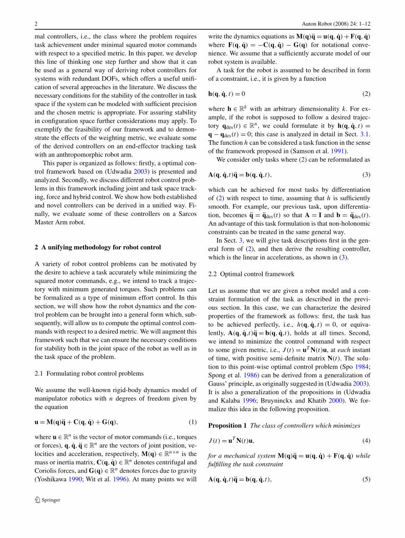
Fig. 3 This figure shows the three end-effector trajectory controllerstracking a “figure eight (8)” pattern at 8 seconds per cycle. On the leftis the x-z plane with the y-z plane on the right. All units are in meters

Fig. 4 The same three controllers tracking the same “figure eight (8)”pattern at a faster pace of 4 seconds per cycle. The labels and unitsremain the same as in Fig. 3

two different speeds. In order to stabilize the null-space tra-jectories, we choose a PD control law in joint space whichpulls the robot towards a fixed rest posture, qrest, given by

u0 = M(KP 0(qrest ! q) ! KD0q).

Additionally we apply gravity, centrifugal and Coriolis forcecompensation, such that u1 = u0 + C + G. For consistency,all three controllers are assigned the same gains both for thetask and joint space stabilization.

Figure 3 shows the end-point trajectories of the three con-trollers in a slow pattern of eight seconds per cycle “figure-eight (8)”. Figure 4 shows a faster pace of four seconds percycle. All three controllers have similar end-point trajecto-ries and result in fairly accurate task achievement. Each onehas an offset from the desired trajectory (thin black line),primarily due to the imperfect dynamics model of the ro-

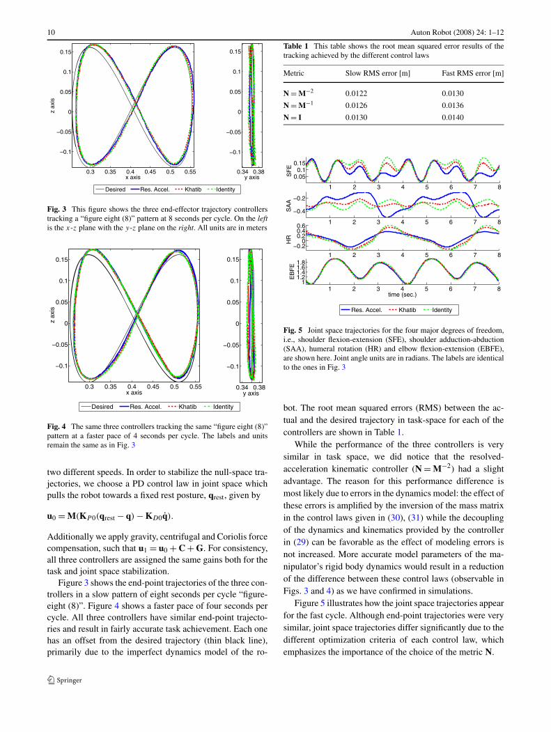
Table 1 This table shows the root mean squared error results of thetracking achieved by the different control laws

Metric Slow RMS error [m] Fast RMS error [m]

N = M!2 0.0122 0.0130

N = M!1 0.0126 0.0136

N = I 0.0130 0.0140

Fig. 5 Joint space trajectories for the four major degrees of freedom,i.e., shoulder flexion-extension (SFE), shoulder adduction-abduction(SAA), humeral rotation (HR) and elbow flexion-extension (EBFE),are shown here. Joint angle units are in radians. The labels are identicalto the ones in Fig. 3

bot. The root mean squared errors (RMS) between the ac-tual and the desired trajectory in task-space for each of thecontrollers are shown in Table 1.

While the performance of the three controllers is verysimilar in task space, we did notice that the resolved-acceleration kinematic controller (N = M!2) had a slightadvantage. The reason for this performance difference ismost likely due to errors in the dynamics model: the effect ofthese errors is amplified by the inversion of the mass matrixin the control laws given in (30), (31) while the decouplingof the dynamics and kinematics provided by the controllerin (29) can be favorable as the effect of modeling errors isnot increased. More accurate model parameters of the ma-nipulator’s rigid body dynamics would result in a reductionof the difference between these control laws (observable inFigs. 3 and 4) as we have confirmed in simulations.

Figure 5 illustrates how the joint space trajectories appearfor the fast cycle. Although end-point trajectories were verysimilar, joint space trajectories differ significantly due to thedifferent optimization criteria of each control law, whichemphasizes the importance of the choice of the metric N.

Auton Robot (2008) 24: 1–12 11

5 Conclusion

In this paper we presented an optimal control frameworkwhich allows the development of a unified approach for de-riving a number of different robot control laws for rigid bodydynamics systems. We demonstrated how we can make useof both the robot model and a task description in order tocreate control laws which are optimal with respect to thesquared motor command under a particular metric whileperfectly fulfilling the task at each instant of time. We havediscussed how to realize stability both in task as well as injoint-space for this framework.

Building on this foundation, we demonstrated how avariety of control laws—which on first inspection appearrather unrelated to one another—can be derived using thisstraightforward framework. The covered types of tasks in-clude joint-space trajectory control for both fully actuatedand overactuated robots, end-effector trajectory control, im-pedance and hybrid control.

The implementation of three of the end-effector trajec-tory control laws resulting from our unified framework ona real-world Sarcos Master Arm robot was carried out as anempirical evaluation. As expected, the behavior in task spaceis very similar for all three control laws; yet, they result invery different joint-space behaviors due to the different costfunctions resulting from the different metrics of each controllaw.

The major contribution of this paper is the unified frame-work that we have developed. It allows a derivation of avariety of previously known controllers, and promises easydevelopment of a host of novel ones, in particular controllaws with additional constraints. The particular controllersreported in this paper were selected primarily for illustrat-ing the applicability of this framework and demonstratingits strength in unifying different control algorithms using acommon building principle. In future work, we will evalu-ate how this framework can yield a variety of new controllaws for underactuated tasks and robots, for non-holonomicrobots and tasks, and for robots with flexible links and joints.

Acknowledgements This research was supported in part by Na-tional Science Foundation grants ECS-0325383, IIS-0312802, IIS-0082995, ECS-0326095, ANI-0224419, a NASA grant AC#98-516,an AFOSR grant on Intelligent Control, the ERATO Kawato DynamicBrain Project funded by the Japanese Science and Technology Agency,and the ATR Computational Neuroscience Laboratories.

References

Arimoto, S. (1996). Control theory of nonlinear mechanical systems: apassivity-based and circuit-theoretic approach. Oxford engineer-ing science series. Oxford: Oxford University Press.

Baillieul, J., & Martin, D. P. (1990). Resolution of kinematic re-dundancy. In Proceedings of symposium in applied mathematics(Vol. 41, pp. 49–89), San Diego, May 1990. Providence: Ameri-can Mathematical Society.

Bruyninckx, H., & Khatib, O. (2000). Gauss’ principle and the dynam-ics of redundant and constrained manipulators. In Proceedings ofthe 2000 IEEE international conference on robotics & automation(pp. 2563–2569).

Chung, W., Chung, W., & Youm, Y. (1993). Null torque based dynamiccontrol for kinematically redundant manipulators. Journal of Ro-botic Systems, 10(6), 811–834.

Craig, J. (1989). Introduction to robotics: mechanics and control. NewYork: Prentice Hall.

Hanafusa, H., Yoshikawa, T., & Nakamura, Y. (1981). Analysis andcontrol of articulated robot with redundancy. In Proceedings ofIFAC symposium on robot control (Vol. 4, pp. 1927–1932).

Hollerbach, J. M., & Suh, K. C. (1987). Redundancy resolution of ma-nipulators through torque optimization. International Journal ofRobotics and Automation, 3(4), 308–316.

Hsu, P., Hauser, J., & Sastry, S. (1989). Dynamic control of redundantmanipulators. Journal of Robotic Systems, 6(2), 133–148.

Isidori, A. (1995). Nonlinear control systems. Berlin: Springer.Kazerounian, K., & Wang, Z. (1988). Global versus local optimization

in redundancy resolution of robotic manipulators. InternationalJournal of Robotics Research, 7(5), 3–12.

Khatib, O. (1987). A unified approach for motion and force controlof robot manipulators: the operational space formulation. IEEEJournal of Robotics and Automation, 3(1), 43–53.

Khatib, O., Sentis, L., Park, J., & Warren, J. (2004). Whole body dy-namic behavior and control of human-like robots. InternationalJournal of Humanoid Robotics, 1(1), 29–43.

Maciejewski, A., & Klein, C. (1985). Obstacle avoidance for kine-matically redundant manipulators in dynamically varying envi-ronments. International Journal of Robotics Research, 4(3), 109–117.

Minamide, N., & Nakamura, K. (1969). Minimum error control prob-lem in Banach space. Research Report of Automatic Control Lab16, Nagoya University, Nagoya, Japan.

Nakamura, Y. (1991). Advanced robotics: redundancy and optimiza-tion. Reading: Addison-Wesley.

Nakamura, Y., Hanafusa, H., & Yoshikawa, T. (1987). Task-prioritybased control of robot manipulators. International Journal of Ro-botics Research, 6(2), 3–15.

Nakanishi, J., Cory, R., Mistry, M., Peters, J., & Schaal, S. (2005).Comparative experiments on task space control with redundancyresolution. In IEEE international conference on intelligent robotsand systems (IROS 2005), Edmonton, Alberta, Canada.

Park, J., Chung, W.-K., & Youm, Y. (1995). Specification and controlof motion for kinematically redundant manipulators. In Proceed-ings international conference of robotics systems.

Park, J., Chung, W.-K., & Youm, Y. (2002). Characterization of in-stability of dynamic control for kinematically redundant manip-ulators. In Proceedings of the IEEE international conference onrobotics and automation.

Pratt, J., & Pratt, G. (1998). Intuitive control of a planar bipedal walk-ing robot. In Proceedings of the 1998 IEEE international confer-ence on robotics & automation (pp. 1024–2021).

Samson, C., Borgne, M. L., & Espiau, B. (1991). Oxford engineeringscience series. Robot control: the task function approach. Oxford:Oxford University Press.

Sciavicco, L., & Siciliano, B. (1996). Modeling and control of robotmanipulators. New York: McGraw-Hill.

Sentis, L., & Khatib, O. (2004). A prioritized multi-objective dynamiccontroller for robots in human environments. In Internationalconference on humanoid robots, Los Angeles, USA. New York:IEEE/RSJ.

Sentis, L., & Khatib, O. (2005). Control of free-floating humanoid ro-bots through task prioritization. In International conference onrobotics and automation (pp. 1730–1735), Barcelona, Spain. NewYork: IEEE.

12 Auton Robot (2008) 24: 1–12

Siciliano, B., & Slotine, J. (1991). A general framework for manag-ing multiple tasks in highly redundant robotic systems. In Inter-national conference on advanced robotics (pp. 1211–1216), Pisa,Italy. New York: IEEE.

Spo (1984). On pointwise optimal control strategies for robot manipu-lators. Princeton: Princeton University Press.

Spong, M., Thorp, J., & Kleinwaks, J. (1986). The control of robot ma-nipulators with bounded input. IEEE Transactions on AutomaticControl, 31(6), 483–490.

Suh, K. C., & Hollerbach, J. M. (1987). Local versus global torque op-timization of redundant manipulators. In Proceedings of the IEEEinternational conference on robotics and automation (pp. 619–624).

Udwadia, F. E. (2003). A new perspective on tracking control ofnonlinear structural and mechanical systems. Proceedings of theRoyal Society of London Series A, 2003, 1783–1800.

Udwadia, F. E., & Kalaba, R. E. (1996). Analytical dynamics: a newapproach. Cambridge: Cambridge University Press.

Wahba, G., & Nashed, M. Z. (1973). The approximate solution of aclass of constrained control problems. In Proceedings of the sixthHawaii international conference on systems sciences, Hawaii.

Wit, C. A. C. D., Siciliano, B., & Bastin, G. (1996). Theory of robotcontrol. Telos: Springer.

Yamane, K., & Nakamura, Y. (2003). Natural motion animationthrough constraining and deconstraining at will constraining anddeconstraining at will. IEEE Transactions on Visualization andComputer Graphics, 9(3).

Yoshikawa, T. (1990). Foundations of robotics: analysis and control.Cambridge: MIT Press.

Jan Peters heads the Robot and ReinforcementLearning Lab (R2L2) at the Max-Planck Insti-tute for Biological Cybernetics (MPI) in Aprilwhile being an invited researcher at the Compu-tational Learning and Motor Control Lab at theUniversity of Southern California (USC). Be-fore joining MPI, he graduated from Universityof Southern California with a Ph.D. in Com-puter Science in March 2007. Jan Peters studiedElectrical Engineering, Computer Science and

Mechanical Engineering. He holds two German M.Sc. degrees in In-formatics and in Electrical Engineering (from Hagen University andMunich University of Technology) and two M.Sc. degrees in ComputerScience and Mechanical Engineering from USC. During his graduatestudies, Jan Peters has been a visiting researcher at the Department ofRobotics at the German Aerospace Research Center (DLR) in Oberp-faffenhofen, Germany, at Siemens Advanced Engineering (SAE) inSingapore, at the National University of Singapore (NUS), and at theDepartment of Humanoid Robotics and Computational Neuroscienceat the Advanced Telecommunication Research (ATR) Center in Kyoto,Japan. His research interests include robotics, nonlinear control, ma-chine learning, and motor skill learning.

Michael Mistry received a B.S.E. degree inElectrical Engineering and Mechanical Engi-neering and Applied Mechanics from the Uni-versity of Pennsylvania in 1998, and an M.Ain Cognitive and Neural Systems from BostonUniversity in 2002. In 2003, he began his Ph.D.studies in Computer Science at the Universityof Southern California (USC) under guidanceof Stefan Schaal. Since then, he has since re-ceived an M.S. in Aerospace and Mechanical

Engineering (2005) and an M.S. in Computer Science (2007) fromUSC. His research currently focuses on the representation, learning,and control of dexterous motor skills in humans and humanoid robots.

Firdaus Udwadia works in the areas of Analyt-ical Dynamics, Nonlinear Dynamical Systems,Structural and Nonlinear Control, and AppliedMathematics. He received his Ph.D. from theCalifornia Institute of Technology. He has pub-lished more than 170 papers in refereed jour-nals, and is the co-author of the book Analyt-ical Dynamics: a new approach, published byCambridge University Press. He is a Fellow ofthe American Society of Mechanical Engineers,

and also a Fellow of the American Institute of Aeronautics and Astro-nautics. In 2006, he received the Outstanding Technical ContributionsAward from the American Society of Civil Engineers.

Jun Nakanishi received the B.E. and M.E.degrees both in mechanical engineering fromNagoya University, Nagoya, Japan, in 1995 and1997, respectively. He received a Ph.D. degreein engineering from Nagoya University in 2000.He also studied in the Department of Electri-cal Engineering and Computer Science at theUniversity of Michigan, Ann Arbor, USA, from1995 to 1996. He was a Research Associate atthe Department of Micro System Engineering,

Nagoya University, from 2000 to 2001, and was a presidential postdoc-toral fellow at the Computer Science Department, University of South-ern California, Los Angeles, USA, from 2001 to 2002. He joined ATRHuman Information Science Laboratories, Kyoto, Japan, in 2002. He iscurrently a researcher at ATR Computational Neuroscience Laborato-ries and with the Computational Brain Project, ICORP, Japan Scienceand Technology Agency. His research interests include motor learningand control in robotic systems. He received the IEEE ICRA 2002 BestPaper Award.

Stefan Schaal is an Associate Professor at theDepartment of Computer Science and the Neu-roscience Program at the University of South-ern California, and an Invited Researcher at theATR Human Information Sciences Laboratoryin Japan, where he held an appointment as Headof the Computational Learning Group during aninternational ERATO project, the Kawato Dy-namic Brain Project (ERATO/JST). Before join-ing USC, Dr. Schaal was a postdoctoral fellow

at the Department of Brain and Cognitive Sciences and the ArtificialIntelligence Laboratory at MIT, an Invited Researcher at the ATR Hu-man Information Processing Research Laboratories in Japan, and anAdjunct Assistant Professor at the Georgia Institute of Technology andat the Department of Kinesiology of the Pennsylvania State Univer-sity. Dr. Schaal’s research interests include topics of statistical andmachine learning, neural networks, computational neuroscience, func-tional brain imaging, nonlinear dynamics, nonlinear control theory, andbiomimetic robotics. He applies his research to problems of artificialand biological motor control and motor learning, focusing on both the-oretical investigations and experiments with human subjects and an-thropomorphic robot equipment.