a unified theory of forward- and backward-looking m&as and divestituressswang/homepage/unified...

A Unified Theory of Forward- and Backward-looking

M&As and Divestitures

Qing Ma and Susheng Wang1

June 2016

Abstract. This paper offers a portfolio explanation to M&As and divestitures. In a unified

theory of forward- and backward-looking M&As and divestitures, an M&A today may be a

cause for a divestiture in the future; conversely a divestiture today may be a consequence of an

M&A in the past. Hence, a decision on an M&A today should consider a possible divestiture in

the future, and a planned divestiture in the future may be dependent on today’s decisions.

M&As and divestitures are not only two sides of the same coin, they are also causes and conse-

quences of each other. In this paper, in a two-period model, two firms consider integrating or

separating in each period. We analyze forward- and backward-looking M&As and divestitures,

and compare them with static M&As and divestitures.

Keywords: unified framework, forward looking, backward looking, M&A, divestiture

JEL classification: G34

1 Address: Hong Kong University of Science and Technology, Clear Water Bay, Hong Kong. Email:

[email protected] and [email protected]. Phone: 852-2358-7600.

2

1. Introduction

In the business world, it is common to see a firm acquiring another firm but later divest-

ing it, or a firm divesting a division but later reacquiring it. Ravenscraft & Scherer (1987) find

that 33% of acquisitions in the 1960s and 1970s were later divested. Porter (1987) finds that

more than half of the acquisitions in new industries were subsequently divested and a startling

74% of the unrelated acquisitions were later divested. He observed that “even a highly respect-

ed company like General Electric divested a very high percentage of its acquisitions.” Kaplan &

Weisbach (1992) also find that, for a sample of large acquisitions during 1971-1982, the ac-

quirers divested almost 44% of the acquired divisions by the end of 1989. Empirical evidence

indicates that firms that merge and then divest often perform well in the interim period, indi-

cating that divestitures are not failures of the past (Allen et al., 1995).

Most of the literature on mergers and acquisitions (M&As) treats M&As and divestitures

as separate strategic decisions (see survey papers by Singh (1993), Johnson (1996), Brauer

(2006), Moschieri & Mair (2008), and Hitt et al. (2009)). The literature has discussed many

possible reasons for M&As and divestitures, including market power, scale economies, risk

aversion, operational synergies, and legal and tax benefits. However, many of these reasons

arguably fail to explain M&As and divestitures, especially since most of the acquired divisions

are later divested. Given that a divested business unit is often one that was acquired in the

past, it is conceivable that when deciding whether or not to acquire a business unit, firms take

into account the possibility of divesting that unit in the future. Conversely, a planned divesti-

ture in the future is likely to be conditional on what the firm decides to do today. Hence, M&As

and divestitures are naturally tied across time in firms’ considerations.

There are relatively few studies focusing on the tied M&As and divestitures which are ac-

tually causes and consequences of each other. Weston (1989) lists 14 reasons for M&As and

divestitures. He concludes that “the data on divestiture/acquisition rates portray a healthy

dynamic interplay between the strategic planning of U.S. companies and continually shifting

market forces”. A popular view in the literature is that “acquirers often buy other firms only to

sell them later”. Porter (1987) finds that most divestitures are successful acquisitions of the

past. Prior literature further points out that the option of divesting an acquired division is

what makes the value of an acquisition positive (Porter, 1987; Weston, 1989; Aron, 1991;

Kaplan & Weisbach, 1992; Shimizu & Hitt, 2005; Fulghieri & Hodrick, 2006) and that the

reacquisition of a divested division is also efficient (Aron, 1991). Fluck & Lynch (1999) theorize

that an acquisition occurs when the acquiree needs funding (e.g. a start-up or distressed firm)

and this acquiree is later divested once its performance has improved sufficiently to allow it to

be standalone again. However, by examining the 1960s conglomerate wave, Hubbard & Pahlia

(1999) find that acquirers neither appear to have higher levels of free cash flows than non-

3

acquirers nor are they punished by the stock market. We argue that two firms may choose to

integrate today simply because they plan to be integrated or to separate in the future or be-

cause they were integrated or separated in the past. Our theory is consistent with both Fluck

and Lynch’s (1999) theory and Hubbard and Pahlia’s (1999) empirical finding.

We develop a two-period model with two firms, a downstream firm (DF) and an up-

stream firm (UF). In this setting, we deal with related M&As and divestitures. Our model is

built on the view that mergers and divestitures are corporate strategies based on internal

characteristics and capabilities and external market conditions. When the firms decide to

integrate or separate in the first period, they will have considered whether to be integrated or

separated in the second period. Similarly, when the firms plan to integrate or separate in the

second period, their plan is affected by what they do now. Without the influence of the deci-

sion in one period, the decision in the other period (called a static solution) can be very differ-

ent. We emphasize the influence of past and expected future decisions. When considering

integration or separation now, whether they are already integrated or separated will obviously

have a major influence. When a decision takes into account another decision in the future, we

call it a forward-looking decision. We also consider backward-looking mergers and divesti-

tures, where a backward-looking decision takes into account a decision made in the past. We

identify forward-looking and backward-looking behavior by comparing a two-period dynamic

solution with a one-period static solution. If we compare a two-period solution with a one-

period solution in the first period, we can identify the forward-looking effect in the two-period

solution. If we compare a two-period solution with a one-period solution in the second period,

we can identify the backward-looking effect in the two-period solution. For example, a back-

ward-looking merger is a merger that is conditional on the fact that the two firms were merged

or separated in the past. We provide a unified model in which both mergers and divestitures

are decisions and both decisions can be forward or backward looking.

Our model has a number of interesting features. First, it is safer to be part of a firm than

to be an independent firm in the competitive market. An upstream division in a firm has the

advantage that there is always a demand for its product. An independent upstream firm faces

the risk of not being able to find a buyer for its product. Second, asset specificity plays a role

when a firm’s status changes from separated to integrated or vice versa. An upstream division

in an integrated firm may have to produce a specific intermediate product for the firm. But

when it is an independent firm in the market, it may have to produce a general product for the

market. This means that the upstream firm may incur adjustment cost when it switches from

being an integrated division to being an independent firm, and vice versa. Due to asset speci-

ficity, there is an adjustment cost for an organizational change. The adjustment cost is a force

working against a reversal of an earlier decision. Hence, the UF changes its status only if the

benefit of doing so is large enough. For more on such adjustment cost in the literature, see

theoretical analysis in Riordan & Williamson (1985) and empirical evidence in Chang and

4

Singh (1999). The use of adjustment cost in our model is consistent with those studies in the

literature that emphasize organizational inertia (Hannan & Freeman, 1984; Amburgey et al.

1993; Shimizu & Hitt, 2005). Third, market fluctuation is a factor in organizational decisions.

Our model takes into account the fact that the market may expand or contract over time. The

firms may decide to change their organizational structure in response to market changes.

Fourth, our model takes into account synergy when the two firms integrate. Synergy under

integration is captured by the condition that the marginal output under integration is larger

than that under separation. Synergy in our model is endogenous in the sense that, when the

two firms merge, their contractual relationship changes accordingly, which affects incentives

and in turn the gain from synergy. Negative synergy is also allowed. In fact, even when nega-

tive synergy and adjustment cost exist, the two firms may choose to integrate if other condi-

tions are ripe for integration. Fifth, incentives are governed by contracts. A contract is a reve-

nue-sharing arrangement offered by a firm’s owners to its manager. We identify the optimal

contract for several common cases. Incentive encourages “effort”, which includes work atti-

tude, work intensity, time spent, and financial investment. The solution from our model offers

an optimal linear contract—a contract that is at least as good as any nonlinear contract. In the

literature, most so-called optimal linear contracts are not optimal since they are strictly inferi-

or to many nonlinear contracts. Sixth, a firm’s internal contractual arrangement is conditional

on its organizational structure. This means that, if the two firms change their organizational

structure, their internal contractual relationship will adjust accordingly. Seventh, managers in

independent firms may have better incentives than divisional managers. A feature specific to

our model is that, the UF’s incentive is better under separation, since the contract under sepa-

ration is based on the UF’s output directly while the contract under integration is related to

the UF’s output indirectly through the DF’s revenue. Eighth, the mood in the marketplace may

affect firms’ decisions. We use a discount factor of time preferences to take into account the

market mood. The firms may decide to integrate early if they feel optimistic now, and they

may decide to separate later if they feel pessimistic now. This discount factor may also be due

to risk aversion to uncertainty in the marketplace. Ninth, our model emphasizes forward

expectations and backward history dependence in firms’ decisions. Tenth, the history is exog-

enous in the “dependence on history” in the literature. However, it is endogenous in our “de-

pendence on the past”. The current decision is a planned decision in the past when the past

decision was made, and the past decision was made conditional on the current decision. In

this sense, we say that the past is endogenous to the current decision. Dependence on endoge-

nous history is fundamentally different from dependence on exogenous history. For example,

market fluctuations have no effect on our forward-looking solutions. The explanation is that,

since a planned decision has already taken into account market fluctuations in the future, it

need not do so again when the time comes to carrying out that decision. Finally, our model is

based on the view that diversification/integration is value enhancing. Some papers in the

literature argue that diversification/integration is value destroying (see Fama (1980), Amihud

5

& Lev (1981), Hart (1983), Jensen & Ruback (1983), Jensen (1986), Shleifer & Vishny (1989),

Jensen & Murphy (1990), and Stulz (1990)). We do not subscribe to the view in the literature

that “divestitures represent failures”. We believe that firms integrate or separate only if doing

so improves their overall profitability.

Our solution is consistent with many empirical findings, and it can explain some seeming-

ly puzzling phenomena. First, our solution includes the case (case IS) in which a firm acquires

another for the purpose of selling it later at a higher value. This is consistent with many stud-

ies in prior literature, including Kaplan and Weisbach’s (1992) observation that on average

targets are divested at 143% of their preacquisition market value, John and Ofek’s (1995)

empirical finding that a typical divested division performs as well as the industry at the time of

divestiture, and Fluck and Lynch’s (1999) theoretical prediction that mergers are followed by

good performance and divestitures. Second, our solution is consistent with the evidence that

diversified firms are less valuable than focused firms (Lang & Stulz, 1994; Berger & Ofek,

1995; Servaes, 1996). In our solution, two firms may choose to integrate or separate due to

past and planned decisions, and not because of current value only. M&As and divestitures may

be value enhancing if we take into account their forward- and backward-looking behavior, but

they may be value destroying if we look at their current value only. Third, firms are often

observed to divest poorly performing divisions (Hayward & Shimizu, 2006). In our solution,

the DF may acquire the UF conditional on a plan to divest it when the latter becomes unprofit-

able due to prevailing market conditions. In this case, the acquirer is shown to have acquired a

poorly performing firm ex post. This is due to the forward-looking behavior, and not because

of entrenchment, mistakes, etc. Fourth, our solution is consistent with two seemingly contra-

dictory empirical findings: (1) mergers increase the combined value of the acquirer and the

target and (2) diversified firms are less valuable than more focused standalone entities. Claim

(1) is based on the stock market reactions when a merger is announced, and hence on ex ante

evaluations. Claim (2) is based on ex post results. We allow a situation in which a firm divests

a division because of a past decision or an expected future decision, and not because of the

division’s current performance. Integration may be value enhancing ex ante by being forward

looking, but it may be value reducing ex post by being backward looking. This can happen, for

example, if integration offers security to acquirees. Also, as will be shown in Proposition 3, an

M&A is likely to happen if substantial synergy exists and firms feel very optimistic now. In

these two examples, the acquisition improves the overall value ex ante, but it may reduce the

overall value ex post.

Our main findings are: Forward- and backward-looking organizational decisions are sub-

stantially different from static ones. The influence of the past is stronger if the market is con-

tracting, if the adjustment cost is larger, or if the time preference for the future is weaker. On

the other hand, the influence of the future is stronger if the adjustment cost is larger, if the

preference for the future is stronger, or if the chance of making deals in the market is lower.

6

Further, in the case where two firms do decide to integrate for a short term, the tendency for

late (early) integration over early (late) integration is stronger if the marginal output under

integration is substantially less than that under separation, if the chance of making deals in

the market is higher, or if the market is expanding sufficiently quickly.

This paper proceeds as follows. Section 2 presents the model. Section 3 derives the solu-

tion. There are four cases: the two firms separate in the first period but reintegrate in the

second period, the two firms integrate in the first period but separate in the second period, the

two firms integrate in the first period and remain integrated in the second period, and the two

firms separate in the first period and remain separated in the second period. Section 4 pre-

sents and analyzes a parametric solution. Section 5 concludes the paper. Finally, the appendix

provides proofs of the results in Section 3 and justifies our choice of the parametric functions

in Section 4.

2. The Model

Consider a two-period model with two firms, a downstream firm (DF) and an upstream

firm (UF). If the two firms are separate, the DF buys input from the market or the UF; if the

two firms are integrated, the DF is the sole user of the UF’s output and the UF is the DF’s

sole supplier.

In practice, the DF is typically the parent firm. Hence, the DF is the principal and the UF

is the agent in our model. This means that if the two firms are integrated, the DF designs and

offers a profit-sharing contract to the UF, and the UF decides whether to take it or leave it. If

the two firms are separate, with probability , the UF receives a purchasing contract from the

DF for its output; with probability , the UF receives no contract. The DF can always buy

the same input from other upstream firms.

The two firms invest into their own production separately. The UF’s investment is denot-

ed by , and the DF’s investment is denoted by . We call them efforts, which includes work

attitude, work intensity, time spent, and financial investment. The costs of efforts for the UF

and DF are respectively and . As is typical in agency problems, these costs are

private, meaning that each party pays for its own cost (not covered in a contract).

Let be the DF’s profit function in period . This profit is the pre-contractual prof-

it, which includes part of the production costs, but not the cost of and . The appendix offers

a more detailed explanation of the pre-contractual profit. The market may expand or contract,

which is an important factor in organizational decisions. The dependence of the profit on time

allows us to incorporate market fluctuations. The firms may decide to change their organiza-

tional relationship in response to the changing market.

7

Let be the UF’s output function under status , where the status can be either

for “integration” or for “separation”. The dependence of the UF’s output on the status

allows us to take into account synergy when the two firms integrate. Synergy exists if the UF’s

marginal output is increased after it is acquired by the DF. Negative synergy is also allowed. In

fact, even when negative synergy and adjustment cost exist, the two firms may choose to inte-

grate if other conditions strongly favor integration.

We incorporate asset specificity in our model. If the two firms are integrated, the UF pro-

duces a relationship-specific product for the integrated firm; if not, it produces a general

product for the market. Suppose there is adjustment cost when the UF switches from

producing a general product to a specific product or vice versa. The UF pays this cost out of its

own pocket. This cost is dependent on its production capacity and the product’s technological

level. We use the UF’s first-period output to represent the production capacity and the DF’s

first-period investment to represent the technological level. Imagine that the UF hires some-

one to adjust machines and production procedures when it switches from producing a specific

product to a general product or vice versa. We expect the marginal cost of this activity to be

diminishing. Hence, we can assume to be concave. This adjustment cost discourages

the UF from changing its status and hence is a force working against a reversal of an earlier

decision.

We also incorporate market risk in our model. A type of market risk is the risk of failing to

make a deal when the UF becomes an independent firm in a competitive market. Given con-

tractual payment , if the UF receives a purchasing contract, its payoff under separation is

where is the probability of having a deal. When there is no deal, there is no payoff. We as-

sume that the DF can always find a supplier of , but the UF may not be able to find a buyer

for its product. Although is given a specific meaning in our model, we can think of as rep-

resenting market risks when the UF is independent in the market.2 Hence, it is safer to be part

of a firm than to be independent in the competitive market. An upstream division in an inte-

grated firm has the advantage that there is always a demand for its product. An independent

UF faces the risk of not being able to find a buyer.

There is a discount factor on the payoff of the second period. This represents the pref-

erence for the future. We may interpret it as representing the market mood. The mood in the

marketplace may affect firms’ decisions. The firms may decide to integrate early if they feel

2 We can easily extend our model to allow and to be dependent on time (the period). Allowing and

to be time-dependent captures the influence of market conditions on them. However, it turns out that these

extensions are unnecessary since our results remain the same.

8

optimistic now, and they may decide to separate later if they feel pessimistic now. We may also

interpret this discount factor as representing risk aversion to uncertainty in the market.

Investments/efforts and are not verifiable, but profit and output and are verifia-

ble ex post. Incentives for investments are provided by contracts. A contract is a profit- or

output-sharing rule. The contract for the UF under separation is the payment to the UF

based on the UF’s output, while the contract ) for the UF under integration is the payment

to the UF based on the DF’s profit.3

When the firms decide to integrate or separate in the first period, they will think/decide

ahead about whether they want to be integrated or separated in the second period. Similarly,

when the firms decide to integrate or separate in the second period, their decision is affected

by what they do now. Such forward- and backward-looking behavior lead to four possibilities:

• Case SI: The two firms are separated in the first period, but integrated in the second period.

• Case IS: The two firms are integrated in the first period, but separated in the second period.

• Case II: The two firms are integrated in both periods.

• Case SS: The two firms are separated in both periods.

There are a few underlying tradeoffs between integration and separation in our model.

First, the UF’s incentive is better under separation, but it faces a risk of having no business

under separation. On the one hand, when the UF is independent, its income is directly related

to its output; this is not so when the UF is acquired by the DF. Hence, the UF has better incen-

tives when it is independent. On the other hand, integration guarantees demand, but there is

no guarantee of demand under separation. Second, the adjustment cost deters organizational

changes, but market risks and fluctuations encourage organizational changes. For example, a

quickly expanding market may induce firms to emphasize incentives so that separation be-

comes a more preferable option.

3. The Four Cases

In this section, we set up the optimization problem for each of the four cases and find its

solution.

3 A more general contract of the form under integration will not change the solution at all.

9

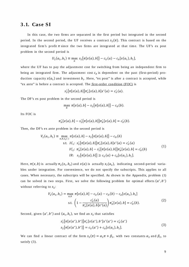
3.1. Case SI

In this case, the two firms are separated in the first period but integrated in the second

period. In the second period, the UF receives a contract . This contract is based on the

integrated firm’s profit since the two firms are integrated at that time. The UF’s ex post

problem in the second period is

where the UF has to pay the adjustment cost for switching from being an independent firm to

being an integrated firm. The adjustment cost is dependent on the past (first-period) pro-

duction capacity and investment . Here, “ex post” is after a contract is accepted, while

“ex ante” is before a contract is accepted. The first-order condition (FOC) is

The DF’s ex post problem in the second period is

Its FOC is

Then, the DF’s ex ante problem in the second period is

, , ⋅

Here, is actually and is actually , indicating second-period varia-

bles under integration. For convenience, we do not specify the subscripts. This applies to all

cases. When necessary, the subscripts will be specified. As shown in the Appendix, problem (1)

can be solved in two steps. First, we solve the following problem for optimal efforts ∗ ∗

without referring to :

,

Second, given ∗ ∗ and , we find an that satisfies ∗ ∗ ∗ ∗ ∗ ∗∗ ∗ ∗We can find a linear contract of the form , with two constants and , to

satisfy (3).

10

In the first period, the two firms are separated. With probability , the DF offers a con-

tract to the UF in the first period based on the UF’s output . Given this contract, the

UF’s ex post problem in the first period is

With probability , the UF cannot find a buyer for its product. The FOC is

,The DF’s ex post problem in the first period is

Its FOC is

,Then, the DF’s ex ante problem in the first period is

, , ⋅ ,,As shown in the Appendix, problem (4) can be solved in two steps. First, we solve the follow-

ing problem for optimal efforts ∗ ∗ without referring to :

, ,Second, given ∗ ∗ , we find an that satisfies ∗ ∗ ∗∗ ∗We can find a linear contract of the form , with two constants and , to

satisfy (6).

3.2. Case IS

In this case, the two firms are integrated in the first period but separated in the second

period. In the second period, with probability , the UF receives a contract . The UF has

to pay the adjustment cost for switching from being an integrated firm to being an independ-

ent firm. The UF’s ex post problem is

Its FOC is

11

The DF’s ex post problem is

Its FOC is

Then, the DF’s ex ante problem is

, , ⋅

As shown in the Appendix, problem (7) can be solved in two steps. We first solve the following

problem for optimal efforts ∗ ∗ without referring to :

,Then, given ∗ ∗ and , we find an that satisfies ∗ ∗ ∗∗ ∗We can find a linear contract of the form , with two constants and , to

satisfy (9).

In the first period, the two firms are integrated. The DF offers a contract based on

its profit to the UF. Given this contract, the UF’s ex post problem is

Its FOC is

,The DF’s ex post problem is

Its FOC is

,Then, the DF’s ex ante problem is

12

, , ⋅ , ,As shown in the Appendix, problem (10) can be solved in two steps. We first solve the follow-


,,

Then, given ∗ ∗ , we find an that satisfies ∗ ∗ ∗ ∗ ∗ ∗∗ ∗ ∗We can find a linear contract of the form , with two constants and , to

satisfy (12).

3.3. Case II

In this case, the two firms are integrated in both periods. In the second period, the DF of-

fers a contract to the UF. Given this contract, the UF’s ex post problem is

Its FOC is


Its FOC is


, , ⋅

As shown in the Appendix, problem (13) can be solved in two steps. We first solve the follow-


13

,


satisfy (15).

In the first period, the two firms are integrated. The DF offers a contract to the UF.

Given this contract, the UF’s ex post problem is

Its FOC is


Its FOC is


, , ⋅



,


satisfy (18).

14

3.4. Case SS

In this case, the two firms are separate in both periods. In the second period, with proba-

bility , the UF receives contract The UF’s ex post problem is

Its FOC is


Its FOC is


, , ⋅



,Then, given ∗ ∗ , we find an that satisfies ∗ ∗ ∗∗ ∗We can find a linear contract of the form , with two constants and , to

satisfy (21).

In the first period, the two firms are also separate. With probability , the UF receives

contract . The UF’s ex post problem is

Its FOC is


15

Its FOC is


, , ⋅


ing problem for optimal effort ∗ ∗ without referring to :

,Then, given ∗ ∗ , we find an that satisfies ∗ ∗ ∗∗ ∗We can find a linear contract of the form , with two constants and , to

satisfy (24).

4. Analysis

According to (37) and (38), we choose the following functional forms for and :

where and are some constants and and are some functions. More specifical-

ly, let

where is the period and is the status, and . Here, the adjustment cost is

concave. This set of parametric functions are rich enough to capture some popular factors

involving mergers and divestitures. For example, synergy under integration is captured by the

condition that the marginal output under integration is larger than that under separation, i.e.,

.

Given this set of functions, the DF’s payoffs for the four cases are

16

Since the UF has no surplus, these payoffs are also the joint payoffs (social welfare) of the two

firms.

We will also consider one-period models. For the one-period model in the first period, we

set in the above solutions and obtain payoffs and for separation and integration,

respectively. These are the payoffs of separation and integration in the first period when there

is no second period. Similarly, for the one-period model in the second period, we obtain pay-

offs and for the two options from in cases SS and II. These payoffs are

We identify forward-looking and backward-looking behavior by comparing a two-period

dynamic solution with a one-period static solution. By comparing a two-period solution with a

one-period solution in the first period, we can identify the forward-looking effect in the two-

period solution. By comparing a two-period solution with a one-period solution in the second

period, we can identify the backward-looking effect in the two-period solution.

4.1. Influence of Past Decisions

Given the decisions in the first period, we now analyze the decisions in the second period.

In the second period, the two firms consider integrating or separating conditional on the

decision made in the first period. That is, the firms’ organizational decisions in the second

period are backward looking. We consider two pairs of comparison:

In the first pair, the first-period status is separation; in the second pair, the first-period status

is integration.

Given First-Period Separation: Cases SI vs. SS

Given that the two firms are separate in the first period, they consider integrating or stay-

ing separate in the second period. We find that if and only if

17

We can draw five conclusions from (28). First, since (28) is more likely to hold if is

larger, given separation in the first period, the tendency for integration in the second period is

stronger if the UF’s marginal output under integration is substantially larger than that under

separation. Second, since (28) is more likely to hold if is smaller, given separation in the first

period, the tendency for integration is stronger in the second period if the chance of making

deals in the market is lower. Third, since (28) is more likely to hold if is smaller, the tenden-

cy for a change of status is stronger in the second period if the adjustment cost is smaller. In

this case, since the two firms are separated in the first period, it is less costly to integrate in the

second period if the adjustment cost is smaller. Fourth, since (28) is more likely to hold if

is larger, given separation in the first period, the tendency for integration is stronger in

the second period if the market is expanding. The explanation is that, with an expanding

market, the agency problem in an integrated firm is lessened. Fifth, since the right-hand side

of (28) is decreasing in , given separation in the first period, the tendency for integration is

stronger in the second period if the preference for the future is stronger (i.e., the discount

factor is larger). That is, when the future is viewed more importantly, the fact that the two

firms are separated in the first period is less of a factor for integration in the second period.

In contrast, if the first period does not exist (or not in consideration), the payoffs are as

defined in (27). We find that if and only if

We can see that it is more difficult for condition (28) than for (29) to hold. By comparing (28)

with (29), we see that the tendency for integration in the second period is weakened (less

likely to be chosen) by the fact that the two firms are separated in the first period. Without the

influence of the first period, the firms are more likely to integrate in the second period. This

influence is represented by the extra multiplier in (28), where the subscript stands for

“first-period separation” and

We make several observations regarding this multiplier. First, when the market expands

( is larger), this multiplier is smaller, implying that second-period integration is less

influenced by first-period separation. The explanation is that, when the market in the second

period is larger than that in the first period, the choice of organizational structure in the sec-

ond period depends less on the past. Second, a larger implies a larger , in turn implying a

larger influence of the first period if adjustment cost rises. The explanation is that, since the

two firms are separated in the first period, a larger adjustment cost boosts the influence of the

18

first period since first-period separation hinders second-period integration through the ad-

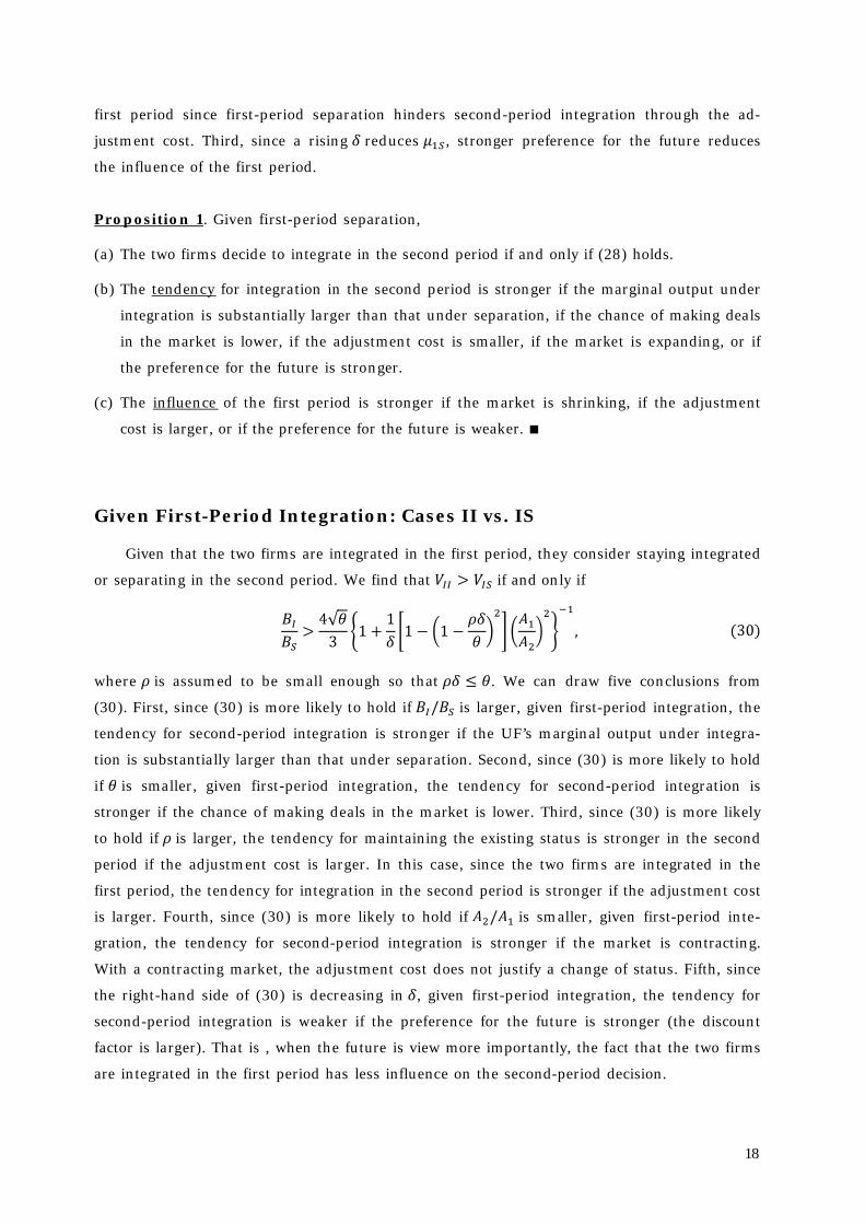
justment cost. Third, since a rising reduces , stronger preference for the future reduces

the influence of the first period.

Proposition 1. Given first-period separation,

(a) The two firms decide to integrate in the second period if and only if (28) holds.

(b) The tendency for integration in the second period is stronger if the marginal output under

integration is substantially larger than that under separation, if the chance of making deals

in the market is lower, if the adjustment cost is smaller, if the market is expanding, or if

the preference for the future is stronger.

(c) The influence of the first period is stronger if the market is shrinking, if the adjustment

cost is larger, or if the preference for the future is weaker.

Given First-Period Integration: Cases II vs. IS

Given that the two firms are integrated in the first period, they consider staying integrated

or separating in the second period. We find that if and only if

where is assumed to be small enough so that . We can draw five conclusions from

(30). First, since (30) is more likely to hold if is larger, given first-period integration, the

tendency for second-period integration is stronger if the UF’s marginal output under integra-

tion is substantially larger than that under separation. Second, since (30) is more likely to hold

if is smaller, given first-period integration, the tendency for second-period integration is

stronger if the chance of making deals in the market is lower. Third, since (30) is more likely

to hold if is larger, the tendency for maintaining the existing status is stronger in the second

period if the adjustment cost is larger. In this case, since the two firms are integrated in the

first period, the tendency for integration in the second period is stronger if the adjustment cost

is larger. Fourth, since (30) is more likely to hold if is smaller, given first-period inte-

gration, the tendency for second-period integration is stronger if the market is contracting.

With a contracting market, the adjustment cost does not justify a change of status. Fifth, since

the right-hand side of (30) is decreasing in , given first-period integration, the tendency for

second-period integration is weaker if the preference for the future is stronger (the discount

factor is larger). That is , when the future is view more importantly, the fact that the two firms

are integrated in the first period has less influence on the second-period decision.

19

In contrast, if the first period does not exist (or not in consideration), the payoffs are as

defined in (27). We find that if and only if (29) holds. We can see that condition (30)

holds more easily than (29). Without the influence of the first period, the two firms are less

likely to integrate in the second period. By comparing (30) with (29), we see that the tendency

for integration is strengthened (more likely to be chosen) by the fact that they are integrated in

the first period. This factor is represented by the extra multiplier in (30), where the sub-

script stands for “first-period integration” and

We make several observations regarding this multiplier. First, when the market expands

( is larger), this multiplier is larger, implying that second-period integration is less

influenced by first-period integration.4 The explanation is that, when the market is expanding,

it makes more sense to maintain the existing organizational structure in the second period.

Second, a larger implies a smaller , in turn implying a larger influence of the first period if

the adjustment cost rises. The explanation is that, since the two firms are integrated in the

first period, it makes more sense to remain integrated in the second period when the adjust-

ment cost is larger. Third, since a rising raises , a higher preference for the future reduces

the influence of the first period. Fourth, since a larger raises , a better chance of making

deals in the market reduces the influence of the first period. A larger encourages separation,

which is against the first-period decision.

We make a further interesting observation by comparing with . Since and

, we see that different first-period decisions have very different influences on second-

period decisions. The fact that means that first-period separation has a negative effect

on second-period integration comparing with that if the first period does not exist (or not in

consideration), while the fact that means that first-period integration has a positive

effect on second-period integration comparing with that if the first period does not exist. That

is, first-period separation hinders second-period integration, while first-period integration

encourages second-period integration. The differential effect of the first period is not

trivially dependent on the adjustment cost. The adjustment cost obviously plays a role, but so

do other factors. For example, if the market contracts, i.e., decreases, the difference

increases, implying a larger differential effect of the first period. On the other hand, if

the market expands quickly, when , we have , meaning that the influence

of the first-period becomes marginal if the market expands quickly. Also, a larger implies a

smaller but a larger , meaning that an increase in the preference for the future reduces

the differential effect of the first period. This is intuitive. As the firms have a stronger prefer-

4 A larger means less influence. When is at its largest possible value, i.e., , the first period has no

influence.

20

ence for the future, the influence of the first period would be reduced. Further, a larger has

no effect on but implies a larger , meaning that a better chance of making deals in the

market reduces the differential effect of the first period. Also, a larger implies a larger

but a smaller , meaning that an increase in the adjustment cost enlarges the differential

effect of the first period.

Proposition 2.

- Given first-period integration,

(a) The two firms decide to integrate in the second period if and only if (30) holds.

(b) The tendency for second-period integration is stronger if the marginal output under in-

tegration is substantially larger than that under separation, if the chance of making

deals in the market is lower if the adjustment cost is larger, if the market is contracting,

or if the preference for the future is weaker.

(c) The influence of the first period is stronger if the market is contracting, if the adjust-

ment cost is larger, if the preference for the future is weaker, or if the chance of making

deals in the market is lower.

- The differential effect of differences in first-period decisions on second-period decisions is

stronger if the market is contracting, if there is less preference for the future, if the chance

of making deals in the market is lower, or if the adjustment cost is larger.

4.2. Influence of Future Decisions

Given the plan in the second period, we now analyze the decisions in the first period. In

the first period, the two firms consider integrating or separating conditional on a plan in the

second period. That is, the firms’ organizational decisions in the first period are forward look-

ing. We consider two pairs of comparison:

In the first pair, the second-period status is separation; in the second pair, the second-period

status is integration.

Conditional on Second-Period Separation: Cases IS vs. SS

Given that the two firms are to be separated in the second period, they consider whether

or not to integrate or separate in the first period. We find that if and only if

21

We can draw four conclusions from (31). First, since (31) is more likely to hold if is

larger, in expectation of second-period separation, the tendency for first-period integration is

stronger if the UF’s marginal output under integration is substantially larger than that under

separation. Second, since (31) is more likely to hold if is smaller, the tendency for a change of

status in the first period is stronger if the adjustment cost is smaller. In this case, since the two

firms plan to be separate firms in the second period, the tendency for first-period integration

is stronger if the adjustment cost is smaller. Third, since (31) is interestingly not affected by

, the tendency for first-period integration is not affected by market fluctuations. The

explanation is that, since the second-period decision has taken into account market fluctua-

tions, the first-period decision needs not do the same. Fourth, since (31) is more likely to hold

if is smaller, the tendency for first-period integration is stronger if the preference for the

future is weaker. The explanation is that, with a weaker preference for the future, second-

period separation has less influence on first-period integration.

In contrast, if there is no second period to speak of (or not in consideration), the payoffs

are as defined by and in (27). We find that if and only if

We can see that it is more difficult for condition (31) than for (32) to hold. By comparing (31)

with (32), we see that the tendency for first-period integration is weakened (less likely to be

chosen) by the fact that the firms are to be separated in the second period. Without the influ-

ence of the second period, the firms are more likely to integrate in the first period. This influ-

ence is represented by the extra multiplier in (31), where the subscript stands for “sec-

ond-period separation” and

We make several observations regarding this multiplier. First, this multiplier is not affected by

changes in , implying that the influence of second-period separation on first-period

integration is not affected by market fluctuations. The explanation is that, since the second-

period decision has already taken into account market fluctuations, the first-period decision

need not do the same. Second, a larger implies a larger , in turn implying a larger influ-

ence of the second period if adjustment cost rises. The explanation is that, since the two firms

are to be separated in the second period, a larger adjustment cost hinders a change of status

and boosts the influence of the second period. Third, since a rising raises , a stronger

preference for the future increases the influence of the future. Fourth, since a larger reduces

, a better chance of making deals in the market reduces the influence of the second period.

The explanation is that, since separation is less costly with a larger , second-best separation

is more likely and hence has less influence on first-period decisions.

22

Proposition 3. In expectation of second-period separation,

(a) The two firms decide to integrate in the first period if and only if (31) holds.

(b) The tendency for first-period integration is stronger if the marginal output under integra-

tion is substantially larger than that under separation, if the adjustment cost is smaller, or

if the preference for the future is weaker. Market fluctuations have no effect on this ten-

dency.

(c) The influence of the second period is stronger if the adjustment cost is larger, if the prefer-

ence for the future is stronger, or if the chance of making deals in the market is lower. This

influence is not affected by market fluctuations.

Conditional on Second-Period Integration: Cases II vs. SI

Given that the two firms are to be integrated in the second period, they consider whether

or not to integrate or separate in the first period. We find that if and only if

We can draw five conclusions from (33). First, since (33) is more likely to hold if is

larger, the tendency for first-period integration is stronger if the UF’s marginal output under

integration is substantially larger than that under separation. Second, since (33) is more likely

to hold if is smaller, in expectation of second-period integration, the tendency for first-

period integration is stronger if the chance of making deals in the market is lower. Third, since

(33) is more likely to hold if is larger, the tendency for first-period integration is stronger if

the adjustment cost is larger. In this case, since the two firms plan to be integrated in the

second period, the tendency for first-period integration is stronger if the adjustment cost is

larger. Fourth, since (33) is interestingly not affected by , the tendency for first-period

integration is not affected by market fluctuations. Since the second-period decision has al-

ready taken into account market fluctuations, the first-period decisions need not do the same.

Fifth, since (33) is more likely to hold if is larger, the tendency for first-period integration is

stronger if the preference for the future is stronger. Given second-period integration and a

stronger preference for the second period, first-period integration makes sense.

In contrast, if there is no second period to speak of (or not in consideration), the payoffs

are as defined by and in (27). We find that if and only if (32) holds. We can see

that condition (33) holds more easily than (32). By comparing (33) with (32), we see that the

tendency for first-period integration is stronger (more likely to be chosen) by the fact that the

firms are to be integrated in the second period. Without the influence of the second period, the

23

firms are less likely to integrate in the first period. This influence is represented by the extra

multiplier in (33), where the subscript stands for “second-period integration” and

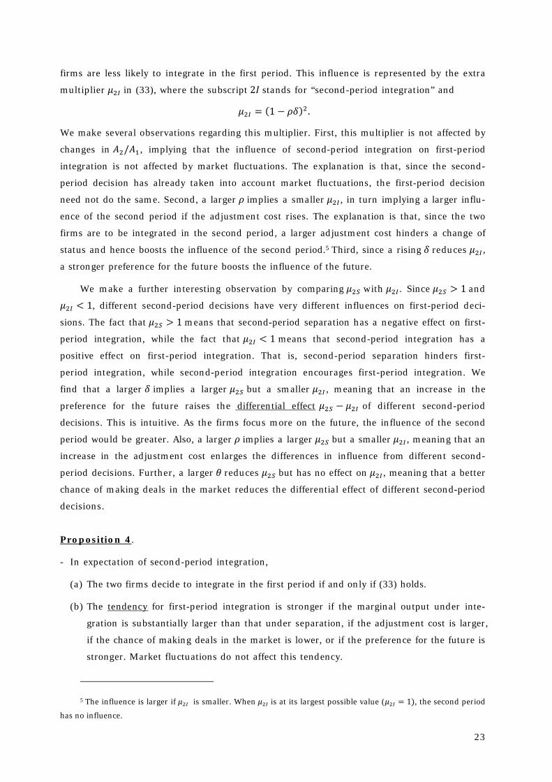
We make several observations regarding this multiplier. First, this multiplier is not affected by

changes in , implying that the influence of second-period integration on first-period

integration is not affected by market fluctuations. The explanation is that, since the second-

period decision has already taken into account market fluctuations, the first-period decision

need not do the same. Second, a larger implies a smaller , in turn implying a larger influ-

ence of the second period if the adjustment cost rises. The explanation is that, since the two

firms are to be integrated in the second period, a larger adjustment cost hinders a change of

status and hence boosts the influence of the second period.5 Third, since a rising reduces ,

a stronger preference for the future boosts the influence of the future.

We make a further interesting observation by comparing with . Since and

, different second-period decisions have very different influences on first-period deci-

sions. The fact that means that second-period separation has a negative effect on first-

period integration, while the fact that means that second-period integration has a

positive effect on first-period integration. That is, second-period separation hinders first-

period integration, while second-period integration encourages first-period integration. We

find that a larger implies a larger but a smaller , meaning that an increase in the

preference for the future raises the differential effect of different second-period

decisions. This is intuitive. As the firms focus more on the future, the influence of the second

period would be greater. Also, a larger implies a larger but a smaller , meaning that an

increase in the adjustment cost enlarges the differences in influence from different second-

period decisions. Further, a larger reduces but has no effect on , meaning that a better

chance of making deals in the market reduces the differential effect of different second-period

decisions.

Proposition 4.

- In expectation of second-period integration,

(a) The two firms decide to integrate in the first period if and only if (33) holds.

(b) The tendency for first-period integration is stronger if the marginal output under inte-

gration is substantially larger than that under separation, if the adjustment cost is larger,

if the chance of making deals in the market is lower, or if the preference for the future is

stronger. Market fluctuations do not affect this tendency.

5 The influence is larger if is smaller. When is at its largest possible value ( , the second period

has no influence.

24

(c) The influence of the second period is stronger if the adjustment cost is larger, or if the

preference for the future is stronger. This influence is not affected by market fluctua-

tions.

- The differential effect of differences in second-period decisions on first-period decisions is

stronger if there is a stronger preference for the future, if the adjustment cost is larger, or if

the chance of making deals in the market is lower.

4.3. Past vs. Future Influences

In the above two sections, we looked at the influences of the past and future separately. In

this section, we allow the firms to consider both influences together.

Suppose the two firms are considering integration or separation today. This decision may

be influenced by the past. If the two firms were integrated in the past, a condition for integra-

tion today is or (30). If the two firms plan to be integrated in the future, a condition

for integration today is or (33). Hence, if the (past, future) status is (integration,

integration), the conditions for integration today are (30) and (33). Similarly, we can analyze

the other three (past, future) statuses and show that conditions

(past, future) status is, the two firms will choose integration today. We find that

conditions are more likely to hold if is larger, is larger, or is small-

er. Also, (28) is more likely to hold if is larger, but (31) is more likely to hold if is smaller. If

is large, the time preference is in favor of today over the past; if is small, the time prefer-

ence is again in favor of today over the future. Hence, when the time preference is in favor of

today, integration is likely to happen today.

Similarly, we find that, if conditions (30) and (33) fail, the two firms will decide to sepa-

rate today irrespective of the past and future. The results are summarized in the following

proposition.

Proposition 5.

(a) If conditions (28) and (31) hold, irrespective of the two firms’ statuses in the past and

future, they will choose integration today, and the tendency for integration today is strong-

er if the marginal output under integration is substantially larger than that under separa-

tion, if the market is expanding, if the adjustment cost is smaller, or if the time preference

is in favor of today.

(b) If conditions (30) and (33) fail, irrespective of the two firms’ statuses in the past and future,

they will choose separation today, and the tendency for separation today is stronger if the

marginal output under integration is substantially less than that under separation, if the

25

market is expanding, if the adjustment cost is smaller, if the chance of making deals in the

market is higher, or if the time preference is in favor of today.

4.4. Short-Term Integration

If the two firms want to be integrated for a short time only (say one period), should they

integrate early or late? Cases SI and IS are about short-term integration, where the former

involves late integration and the latter early integration.

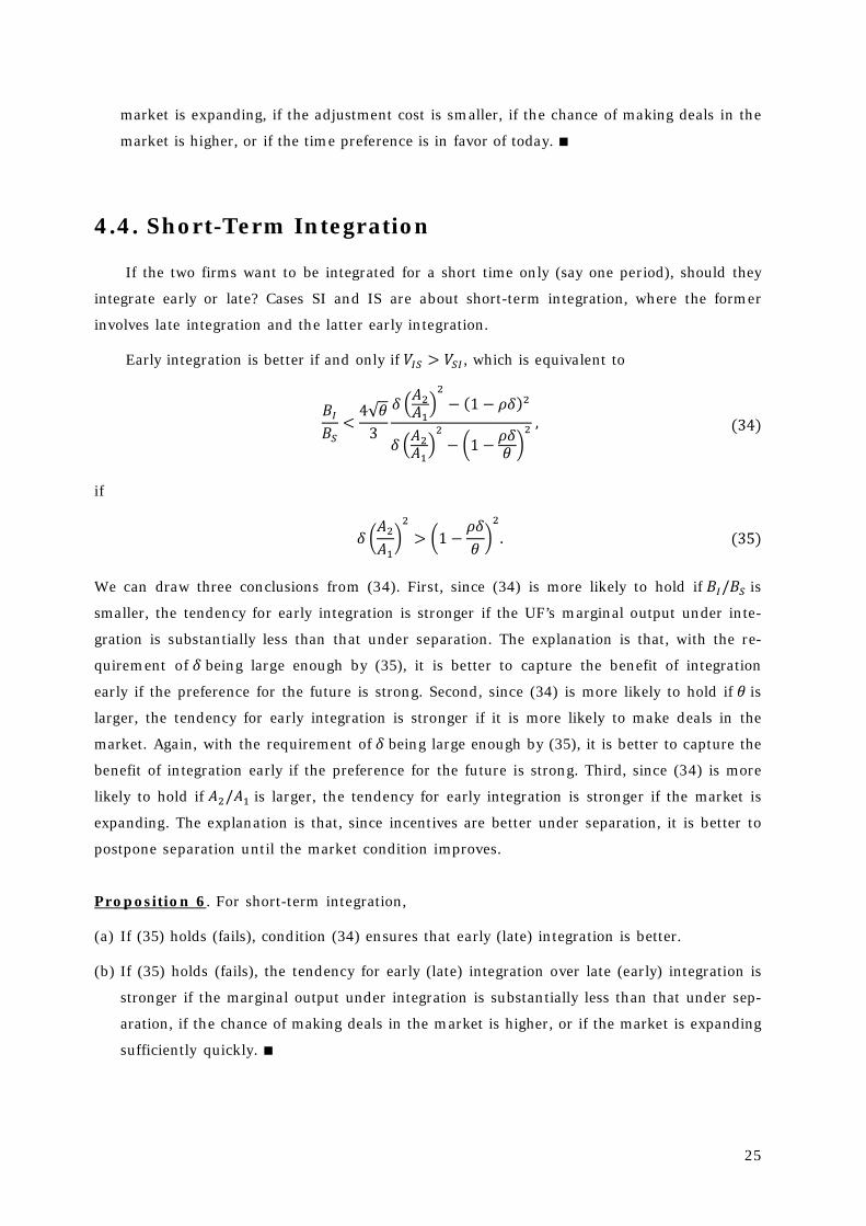
Early integration is better if and only if , which is equivalent to

if

We can draw three conclusions from (34). First, since (34) is more likely to hold if is

smaller, the tendency for early integration is stronger if the UF’s marginal output under inte-

gration is substantially less than that under separation. The explanation is that, with the re-

quirement of being large enough by (35), it is better to capture the benefit of integration

early if the preference for the future is strong. Second, since (34) is more likely to hold if is

larger, the tendency for early integration is stronger if it is more likely to make deals in the

market. Again, with the requirement of being large enough by (35), it is better to capture the

benefit of integration early if the preference for the future is strong. Third, since (34) is more

likely to hold if is larger, the tendency for early integration is stronger if the market is

expanding. The explanation is that, since incentives are better under separation, it is better to

postpone separation until the market condition improves.

Proposition 6. For short-term integration,

(a) If (35) holds (fails), condition (34) ensures that early (late) integration is better.

(b) If (35) holds (fails), the tendency for early (late) integration over late (early) integration is

stronger if the marginal output under integration is substantially less than that under sep-

aration, if the chance of making deals in the market is higher, or if the market is expanding

sufficiently quickly.

26

4.5. Contractual Analysis

From the analysis in Section 3, there is an optimal linear contract of the form

or in each of the four cases. From conditions (3), (6), (9), (12), (15),

(18), (21) and (24), we know that the constant is designed to satisfy the IC condition, and

the constant is designed to satisfy the IR condition. represents a one-time transfer be-

tween the two parties, which does not affect incentives, while represents how the two par-

ties share ex-post output or profit, which offers incentives. Hence, our interest is in the income

sharing rule . Given the set of functions in (25), the income sharing rules for the four cases

are

∗ ∗∗ ∗∗ ∗∗ ∗

We make several observations regarding the income sharing rule ∗. First, the contractual

terms are dependent on the organizational structure. In different organizational arrangements,

contractual terms differ. Second, when the two firms are separate, the income sharing rule is

dependent on market conditions, and the dependence is interestingly characterized by a

common factor . Only when a change of status in the future is expected, an extra

term is used to take into account the adjustment cost. Third, when the two firms are inte-

grated, if a change of status in the future is not expected, the income sharing rule is ∗ ,

i.e., they share profit equally. However, as shown in case IS, the income sharing rule under

integration in the first period uses an extra term when a change of status is expected,

where the extra term takes into account the adjustment cost and the chance of making deals in

the market when the UF becomes separated in the second period. Fourth, in expectation of a

change of status in the second period, the UF’s first-period income share is reduced comparing

to that if there is no future organizational change.

5. Concluding Remarks

An M&A may be due to an earlier divestiture or a planned future one. Similarly, a divesti-

ture may occur following an earlier M&A or a planned future one. When a firm considers

acquiring another, the option to divest the acquiree in the future is an important considera-

tion; on the other hand, the fact that the acquirer had once divested this acquiree (but is trying

27

to reacquire it now) is also an important factor. Given these considerations, this paper focuses

on forward- and backward-looking M&As and divestitures.

Prior literature has never discussed the influence of past and future decisions on current

decisions. As we have shown, forward- and backward-looking behaviors have major influences

on current decisions. We have built a dynamic vertical integration model, which has never

been seen in prior literature. In such a model, asset specificity and adjustment cost play im-

portant roles in mergers and divestitures.

Our main findings are: Forward- and backward-looking organizational decisions are sub-

stantially different from static ones. The influence of the first period is stronger if the market is

contracting, if the adjustment cost is larger, or if the preference for the future is weaker. On

the other hand, the influence of the second period is stronger if the adjustment cost is larger, if

the preference for the future is stronger, or if the chance of making deals in the market is

lower. Further, in the case where two firms choose to be integrated for a short time, the ten-

dency for early (late) integration over late (early) integration is stronger if the marginal output

under integration is substantially less than that under separation, if the chance of making

deals in the market is higher, or if the market is expanding sufficiently quickly.

Our paper offers a unified theory covering four cases. These four cases encompass three

patterns of mergers and divestitures that are often observed in practice. The first case is re-

peated integration and separation: two firms choose to integrate but later decide to separate

(case IS); after a while, they decide to integrate again (case SI). The second case is permanent

separation: two firms decide to separate (case IS) and to remain separated forever (case SS).

The third case is permanent integration: two firms decide to integrate (case SI) and to remain

integrated forever (case II). Prior studies have discussed either case IS or case SI, but they

were always treated as two unrelated cases. We extend prior studies by analyzing these two

cases in the same model.

Appendix

A.1. The General Solution

This section offers proofs of the solutions for the four cases in Section 3.

The Solution for Case SI

For both problems (1) and (4), if the IR condition is not binding, the DF can always offer

for some instead of to satisfy the IR condition. Hence, the IR condition

must be binding in equilibrium.

In the second period, by the binding IR condition, problem (1) becomes

28

, , ⋅

Utilizing for , this problem can be transformed into

, , ⋅

Since does not appear in the objective function of problem (36), it can be solved using

(2) and (3).

In the first period, since the UF has no surplus in the second period (a binding IR condi-

tion), we have . For problem (4), with a binding IR condition, problem (4) be-

comes

, , ⋅,

Since does not appear in the objective function, it can be solved using (5) and (6).

The Solution for Case IS

In the second period, it is easy to see that the IR condition in (7) must be binding. Hence,

problem (7) can be rewritten as

, , ⋅

Since does not appear in the objective function, this problem can be solved using (8) and

(9).

In the first period, it is also easy to see that the IR condition in (10) must be binding.

Hence, problem (10) can be rewritten as

29

, , ⋅,

Since does not appear in the objective function, this problem can be solved using (11)

and (12).

The Solution for Case II



, , ⋅


and (15).



, , ⋅


and (18).

The Solution for Case SS



, , ⋅

Since does not appear in the objective function, this problem can be solved using(20)

and (21).

30



, , ⋅


and (24).

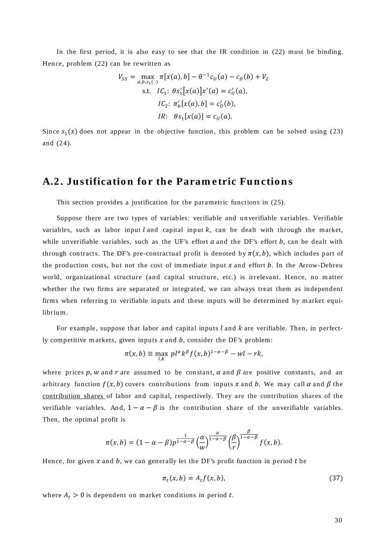
A.2. Justification for the Parametric Functions

This section provides a justification for the parametric functions in (25).

Suppose there are two types of variables: verifiable and unverifiable variables. Verifiable

variables, such as labor input and capital input , can be dealt with through the market,

while unverifiable variables, such as the UF’s effort and the DF’s effort , can be dealt with

through contracts. The DF’s pre-contractual profit is denoted by , which includes part of

the production costs, but not the cost of immediate input and effort . In the Arrow-Debreu

world, organizational structure (and capital structure, etc.) is irrelevant. Hence, no matter

whether the two firms are separated or integrated, we can always treat them as independent

firms when referring to verifiable inputs and these inputs will be determined by market equi-

librium.

For example, suppose that labor and capital inputs and are verifiable. Then, in perfect-

ly competitive markets, given inputs and , consider the DF’s problem:

,where prices , and are assumed to be constant, and are positive constants, and an

arbitrary function covers contributions from inputs and . We may call and the

contribution shares of labor and capital, respectively. They are the contribution shares of the

verifiable variables. And, is the contribution share of the unverifiable variables.

Then, the optimal profit is

Hence, for given and , we can generally let the DF’s profit function in period be

where is dependent on market conditions in period .

31

We can similarly consider the UF’s problem. Again, since a firm’s organizational structure

is irrelevant in competitive markets, no matter whether the UF is separated or integrated, we

can always treat it as an independent firm when referring to verifiable inputs. Hence, in per-

fectly competitive markets, given input , the UF’s problem for verifiable inputs is

,where prices , and and parameters and may not be the same as those in the DF’s

problem above. We use the same notation for convenience. Let ∗ and ∗ be the optimal inputs.

Then, the optimal output is

∗ ∗ and the optimal profit is

Hence, we can generally let the UF’s production function under status be

for some constant , where is dependent on market conditions under status .

References

Allen, J.W.; Lummer, S.L.; McConnell, J.T.; Reed, D.K. (1995). Can Takeover Losses Ex-

plain Spin-Off Gains? Journal of Financial and Quantitative Analysis, 30 (4), 465-485.

Amburgey, T.L.; Kelly, D.; Barnett, W.P. 1993. Resetting the clock: The dynamics of or-

ganizational change and failure. Administrative Science Quarterly, 38, 51-73.

Amihud, Y.; Lev, B. 1981. Risk reduction as a managerial motive for conglomerate mer-

gers. Bell Journal of Economics, 12, 605-617.

Aron, D.J. 1991. Using the Capital Market as a Monitor: Corporate Spinoffs in an Agency

Framework. RAND Journal of Economics, 22 (4), 505-518.

Berger, P.G.; Ofek, E. 1995. Diversification’s effect on firm value. Journal of Financial

Economics, 37, 39-65.

Brauer, M. 2006. What Have We Acquired and What Should We Acquire in Divestiture

Research? A Review and Research Agenda. Journal of Management, 32 (6), 751-785.

32

Chang, S.J.; Singh, H. 1999. The Impact of modes of entry and resource fit on modes of

exit by multibusiness firms. Strategic Management Journal, 20, 1019-1035.

Fama, E. 1980. Agency problems and the theory of the firm. Journal of Political Econo-

my, 88, 288-307.

Fluck, Z.; Lynch, A.W. 1999. Why Do Firms Merge and Then Divest? A Theory of Finan-

cial Synergy. Journal of Business, 72 (3), 319-346.

Fulghieri, P.; Hodrick, L.S. 2006. Synergies and Internal Agency Conflicts: The Double-

Edged Sword of Mergers. Journal of Economics & Management Strategy, 15 (3), 549-576.

Hannan, M.; Freeman, J. 1984. Structural inertia and organizational change. American

Sociological Review, 49, 149-164.

Hart, O. 1983. The market mechanism as an incentive scheme. Bell Journal of Economics,

14, 366-382.

Hayward, M.L.A.; Shimizu, K. 2006. De-commitment to losing strategic action: Evidence

from the divestiture of poorly performing acquisitions. Strategic Management Journal, 27

(6), 541-557.

Hitt, M.A.; King, D.; Krishnan, H.; Makri, M.; Schijven, M.; Shimizuf, K.; Zhu, H. 2009.

Mergers and acquisitions: Overcoming pitfalls, building synergy, and creating value. Business

Horizons, 52, 523-529.

Hubbard, G.; Pahlia, D. 1999. A re-examination of the conglomerate merger wave in the

1960s: An internal capital market view. Journal of Finance, 54 (3), 1131-1152.

Jensen, M. 1986. Agency costs of free cash flows, corporate finance and takeovers. Ameri-

can Economic Review, 76, 323-329.

Jensen, M.; Murphy, K. 1990. Performance pay and top management incentives. Journal

of Political Economy, 98, 225-263.

Jensen, M.C.; Ruback, R.S. 1983. The market for corporate control: A scientific evidence.

Journal of Financial Economics, 11, 5-50.

John, K.; Ofek, E. 1995. Asset sales and increase in focus. Journal of Financial Econom-

ics, 37, 105-126.

Johnson, R.A. 1996. Antecedents and Outcomes of Corporate Refocusing. Journal of

Management, 22 (3), 439-483.

Kaplan, S.N.; Weisbach, M.S. 1992. The success of acquisitions: Evidence from divesti-

tures. Journal of Finance, 47, 107-138.

Lang, L.; Stulz, R. 1994. Tobin’s q, corporate diversification and firm performance. Jour-

nal of Political Economy, 102, 1248-1280.

33

Moschieri, C.; Mair, J. 2008. Research on corporate divestitures: A synthesis. Journal

of Management & Organization, 14, 399-422.

Porter, M. 1987. From competitive advantage to corporate strategy. Harvard Business

Review, January, 43-59.

Ravenscraft, D.; Scherer, F.M. 1987. Mergers, Selloffs and Economic Efficiency. Wash-

ington, D.C., Brookings.

Riordan, M.H.; Williamson, O.E. 1985. Asset specificity and economic organization. In-

ternational Journal of Industrial Organization, 3, 365-378.

Servaes, H. 1996. The value of diversification during the conglomerate merger wave.

Journal of Finance, 51, 1201-1226.

Shimizu, K.; Hitt, M.A. 2005. What Constrains or Facilitates Divestitures of Formerly Ac-

quired Firms? The Effects of Organizational Inertia. Journal of Management, 31 (1), 50-72.

Shleifer, A.; Vishny, R. 1989. Management entrenchment: The case of manager-specific

investment. Journal of Financial Economics, 25, 123-139.

Singh, H. 1993. Challenges in Researching Corporate Restructuring. Journal of Manage-

ment Studies, 30 (1), 147-172.

Stulz, R. 1990. Managerial discretion and optimal financing policies. Journal of Financial

Economics, 26, 3-27.

Weston, J.F. 1989. Divestitures: Mistakes or Learning. Journal of Applied Corporate Fi-

nance, 2 (2), 68-76.

a unified theory of forward- and backward-looking m&as and divestituressswang/homepage/unified...

Documents