Federal Reserve Bank of MinneapolisResearch Department Staff Report 346

September 2004

A Unified Framework for MonetaryTheory and Policy Analysis∗

Ricardo Lagos

New York Universityand Federal Reserve Bank of Minneapolis

Randall Wright

University of Pennsylvaniaand Federal Reserve Bank of Cleveland

ABSTRACT

Search-theoretic models of monetary exchange are based on explicit descriptions of the frictions thatmake money essential. However, tractable versions of these models typically need strong assumptionsthat make them ill-suited for studying monetary policy. We propose a framework based on explicitmicro foundations within which macro policy can be analyzed. The model is both analyticallytractable and amenable to quantitative analysis. We demonstrate this by using it to estimate thewelfare cost of inflation. We find much higher costs than the previous literature: our model predictsthat going from 10% to 0% inflation can be worth between 3% and 5% of consumption.

∗First version: May 2000. Many people provided extremely helpful input to this project, including S.B. Aruoba,A. Berentsen, V.V. Chari, L. Christiano, N. Kocherlakota, G. Rocheteau, S. Shi, C. Waller, and N. Wallace.Financial support from the C.V. Starr Center for Applied Economics at NYU, STICERD at the LSE, theNSF, and the Federal Reserve Banks of Cleveland and Minneapolis is acknowledged. The views expressedherein are those of the authors and not necessarily those of the Federal Reserve Bank of Cleveland, the FederalReserve Bank of Minneapolis, or the Federal Reserve System.

1 Introduction

Existing monetary models in macroeconomics are reduced-form models. By

this we mean they make assumptions, such as putting money in the utility

function or imposing cash-in-advance constraints, that are meant to stand in

for some role of money that is not made explicit–say, that it helps overcome

spatial, temporal, or informational frictions. There are models that provide

micro foundations for monetary economics using search theory, based on ex-

plicit descriptions of specialization, the pattern of meetings, the information

structure, and so on. This framework can be used to address issues such

as: what types of frictions make the use of money an equilibrium or effi-

cient arrangement; which objects endogenously end up serving as media of

exchange; or how do different regimes (e.g., commodity versus fiat money, or

one currency versus two) lead to different outcomes. But these models are

ill suited for the analysis of monetary policy as it is usually formulated. The

reason is that the typical search-based model becomes intractable without

very strong assumptions, including extreme restrictions on how much money

agents can hold. Therefore, if one wants to study policy there is little choice

but to resort to the reduced-form approach.1

In this paper we propose a framework that attempts to bridge this gap:

it is based explicitly on microeconomic frictions and can be used to study a

range of macroeconomic policies. As an application we carry out a quantita-

tive analysis of the welfare cost of inflation. This exercise clearly illustrates

1In terms of the literature, examples of reduced-form models include Lucas and Stokey(1983, 1987), Cooley and Hansen (1989, 1991), and Christiano et al. (1997); see Walsh(1998) for more references. Examples in the search literature with strong assumptions onmoney holdings include Kiyotaki and Wright (1989, 1991), Shi (1995), Trejos and Wright(1995), Kocherlakota (1998), and Wallace (2001). Other search models are discussedbelow.

1

that, besides being analytically tractable, the model can also be realistically

parametrized. We find much higher welfare costs than the previous litera-

ture: our model predicts that going from 10% to 0% inflation can be worth

between 3% and 5% of consumption.

There are previous attempts to study search models without severe re-

strictions on money holdings, m. Trejos and Wright (1995) present a version

of their model where agents can hold anym ∈ R+, but cannot solve it and endup resorting tom ∈ 0, 1. The model withm ∈ R+ is studied numerically byMolico (1999). Although his findings are interesting, the framework is very

complicated: basically no analytic results are available and even numerical

analysis is difficult. What makes the problem complicated is the endogenous

distribution of money holdings, F (m). Our model integrates decentralized

trade as in search theory with periodic access to centralized markets. For a

certain class of preferences, we find that all agents in the centralized market

choose the same money balances, which renders F degenerate in the decen-

tralized market.2 The model in Shi (1997) is related to our framework and

also gets F degenerate, although by different means. We will compare these

different approaches in considerable detail below, after describing how our

model works.

The rest of the paper is organized as follows. Section 2 describes the

environment. Section 3 defines equilibrium and derives some basic results.

2The relevant class of preferences displays a certain quasi-linearity. Intuitively, quasi-linearity implies the amount of money you take to the market today does not dependon how much you came home with last night. We suggest below that this may not bea bad empirical approximation, but the main advantage is really analytic convenience.Another argument for quasi-linear preferences, however, is that they are used in manyother macroeconomic applications, including much real business cycle theory and reduced-form monetary economics; examples include Hansen (1985), Rogerson (1988), Cooley andHansen (1989, 1991), and Christiano and Eichenbaum (1992).

2

Section 4 discusses the related literature, including Shi (1997). Section 5 in-

troduces monetary policy considerations. Section 6 uses a calibrated version

to quantify the welfare cost of inflation. Section 7 concludes. The Appendix

contains many technical results.

2 The Model

Time is discrete. There is a [0, 1] continuum of agents who live forever with

discount factor β ∈ (0, 1). Each period is divided into two subperiods, dayand night. Agents consume and supply labor in both subperiods. In general,

preferences are U(x, h,X,H), where x and h (X and H) are consumption

and labor during the day (night). It is important for tractability that U islinear in either X or H. We assume

U(x, h,X,H) = u(x)− c(h) + U(X)− AH,

although separability across (x, h,X) is not critical and is made merely to

ease the presentation. Assume u, c, and U are Cn (n times continuously

differentiable) with n ≥ 2. Also, assume U 0 > 0, U 00 ≤ 0, U is either

unbounded or satisfies a condition in Lemma 6, and there exists X∗ ∈ (0,∞)such that U 0(X∗) = 1 and U(X∗) > X∗. Also, assume u(0) = c(0) = 0,

u0 > 0, c0 > 0, u00 < 0, c00 ≥ 0, and there exists q∗ ∈ (0,∞) such thatu0(q∗) = c0(q∗).

Economic activity differs across the subperiods. As in the typical search

model, during the day agents interact in a decentralized market involving

anonymous bilateral matching with arrival rate α. We assume the day good

x comes in many specialized varieties, of which each agent consumes only

a subset. An agent can transform labor one for one into a special good

3

that he does not consume. This generates a double coincidence problem. In

particular, for two agents i and j, drawn at random, there are four possible

events. The probability that both consume what the other can produce (a

double coincidence) is δ. The probability that i consumes what j produces

but not vice versa (a single coincidence) is σ. Symmetrically, the probability

j consumes what i produces but not vice versa is σ. And the probability

that neither wants what the other produces is 1− 2σ− δ, where 2σ ≤ 1− δ.3

In a single coincidence meeting, if i wants the special good that j produces,

we call i the buyer and j the seller.

At night agents trade in a centralized (Walrasian) market. With central-

ized trade, specialization does not lead to a double coincidence problem, and

so it is irrelevant if the night good X comes in many varieties or only one;

hence we assume that at night all agents produce and consume a general

good, mainly because this allows a closer comparison with standard macro

models. Agents at night can transform 1 unit of labor into w units of the

general good, where we assume here that w is a technological constant, and

be normalized to w = 1 with no loss in generality.4 We assume the general

goods produced at night and the special goods produced during the day are

nonstorable. There is another object, called money, that is perfectly divisible

and can be stored in any quantity m ≥ 0.3This notation captures several specifications in the literature as special cases. In

Kiyotaki and Wright (1989) or Aiyagari and Wallace (1991) there are N goods and Ntypes, and type n produces good n and consumes good n+1, modN . If N > 2, σ = 1/Nand δ = 0, while if N = 2, δ = 1/2 and σ = 0. In Kiyotaki and Wright (1993) theevent that i consumes what j produces is independent of the event that j consumes whati produces, and each occurs with probability x. Then δ = x2 and σ = x(1− x).

4Aruoba and Wright (2003) show how to recast things in terms of agents selling laborto neoclassical firms for w units of purchasing power, where w is determined to clear thelabor market; this changes nothing of substance.

4

Figure 1: Timing

This completes the description of the physical environment. The timing is

illustrated in Figure 1. Given our assumptions, the only feasible trades during

the day are barter in special goods and the exchange of special goods for

money, and at night the only feasible trades involve general goods and money;

special goods can never be traded at night nor general goods during the

day because they are only produced in one subperiod and are not storable.5

Therefore, in this model money is essential for the same reason it is in the

typical search-based model: since meetings in the day market are anonymous

there is no scope for trading future promises, so exchange must be quid pro

quo.6 Notice, however, that from an individual’s point of view it is by no

means necessary to use money–he could always try to barter special goods

directly. It is rather that he may choose to use money because this may make

exchange easier.

5Lagos and Rocheteau (2003) consider an extension where general goods are storableand hence potentially compete with fiat money as a medium of exchange. Although goodsare not storable here, we can allow the exchange of intertemporal claims across meetingsof the centralized market. Since agents will be homogeneous, as is standard, such claimswill not trade but we can still price assets, including real and nominal bonds.

6In this context when one says that money is essential it means the economy is able toachieve more outcomes (or better outcomes) with money than without; see Kocherlakota(1998) and Wallace (2001).

5

3 Equilibrium

In this section we build gradually towards the definition of equilibrium. We

begin by describing the value functions, taking as given the terms of trade

and the distribution of money. In general, the state variable for an individual

includes his own money holdings m and a vector of aggregate states s. At

this point we let s = (φ, F ), where φ is the value of money in the centralized

market (pg = 1/φ is the nominal price at night) and F is the distribution of

money holdings in the decentralized market (F (m) is the measure of agents

in the day market holdingm ≤ m). For now the total money stock is fixed at

M , and soRmdF (m) =M at every date; we consider changes in the money

supply (both deterministic and stochastic) in Section 5. The agent takes as

given a law of motion s+1 = Υ(s), but it will be determined endogenously in

equilibrium.7

Let V (m, s) be the value function for an agent with m dollars in the

morning when he enters the decentralized market, and W (m, s) the value

function in the afternoon when he enters the centralized market. In a single-

coincidence meeting, since the seller’s production h must equal the buyer’s

consumption x, we denote their common value by q (m, m, s), and denote the

dollars that change hands by d (m, m, s), where in general these may both

depend on the money holdings of the buyer m and the seller m as well as the

aggregate state s. In a double-coincidence meeting, we denote by B(m, m, s)

the payoff for an agent with m who meets an agent with m. Bellman’s

7Putting φ in the state vector allows us to capture nonstationary equilibria using re-cursive methods (Duffie et al. [1994] use a similar approach in overlapping generationsmodels). In any case, for much of this paper we will focus on steady states, so this is notan issue.

6

equation is8

V (m, s) = ασ

Zu [q (m, m, s)] +W [m− d (m, m, s)] dF (m)

+ασ

Z−c [q (m,m, s)] +W [m+ d (m,m, s)] dF (m) (1)

+αδ

ZB(m, m, s)dF (m) + (1− 2ασ − αδ)W (m, s).

The value of entering the centralized market with m dollars is

W (m, s) = maxX,H,m+1

U (X)− AH + βV (m+1, s+1) (2)

s.t. X = H + φm− φm+1

where m+1 is money taken out of this market.9 Normalizing A = 1 and

substituting for H,

W (m, s) = φm+ maxX,m+1

U(X)−X − φm+1 + βV (m+1, s+1) . (3)

This immediately implies several things. First, X = X∗ where U 0(X∗) = 1.

Second, we have the convenient result that m+1 does not depend on m;

intuitively, the quasi-linearity of U rules out wealth effects in the choice ofm+1. Third, we have the result that W is linear in m,

W (m, s) =W (0, s) + φm. (4)

Now that we have the value functions, consider the terms of trade in the

decentralized market, which are determined by bargaining. There are two

8The first term is the expected payoff from a single-coincidence meeting where you buyq (m, m, s) and proceed to the centralized market with m− d (m, m, s) dollars. The otherterms have similar interpretations.

9While standard curvature conditions can be used to guarantee, for example, X > 0, wecannot so easily rule out corner solutions for H because of quasi-linearity. Our approachis to simply assume an interior solution for H for now, and impose conditions later toguarantee that this is valid.

7

bargaining situations to consider: single- and double-coincidence meetings.

In the latter case we adopt the symmetric Nash bargaining solution with the

threat point of an agent given by his continuation value W (m, s). Lemma

1 in the Appendix proves that, regardless of the money holdings of the two

agents, in any double-coincidence meeting they give each other the efficient

quantity q∗ defined by u0(q∗) = c0(q∗), and no money changes hands. Thus,

B(m, m, s) = u(q∗)− c(q∗) +W (m, s).

Now consider bargaining in a single-coincidence meeting when the buyer

has m and the seller m dollars. Here we use the generalized Nash solu-

tion where the buyer has bargaining power θ and threat points are given by

continuation values.10 Hence (q, d) maximizes

[u (q) +W (m− d, s)−W (m, s)]θ [−c (q) +W (m+ d, s)−W (m, s)]1−θ

subject to the feasibility constraint d ≤ m. By (4) this simplifies nicely to

maxq,d

[u (q)− φd]θ [−c (q) + φd]1−θ (5)

subject to d ≤ m.

Notice (5) does not depend on m at all, and depends on m iff the con-

straint d ≤ m binds. Also, it depends on s only through φ, and indeed

only through real balances z = φm. We write q(m, m, s) = q(m) and

d(m, m, s) = d(m) in what follows (the dependence on φ is implicit). Lemma

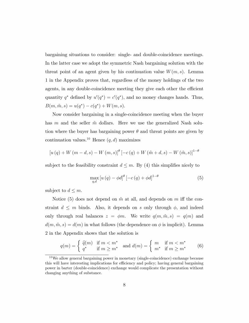
2 in the Appendix shows that the solution is

q(m) =

½ bq(m) if m < m∗

q∗ if m ≥ m∗ and d(m) =

½m if m < m∗

m∗ if m ≥ m∗ (6)

10We allow general bargaining power in monetary (single-coincidence) exchange becausethis will have interesting implications for efficiency and policy; having general bargainingpower in barter (double-coincidence) exchange would complicate the presentation withoutchanging anything of substance.

8

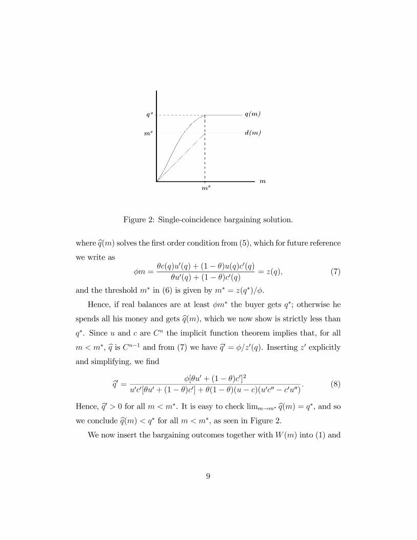
Figure 2: Single-coincidence bargaining solution.

where bq(m) solves the first order condition from (5), which for future referencewe write as

φm =θc(q)u0(q) + (1− θ)u(q)c0(q)

θu0(q) + (1− θ)c0(q)= z(q), (7)

and the threshold m∗ in (6) is given by m∗ = z(q∗)/φ.

Hence, if real balances are at least φm∗ the buyer gets q∗; otherwise he

spends all his money and gets bq(m), which we now show is strictly less thanq∗. Since u and c are Cn the implicit function theorem implies that, for all

m < m∗, bq is Cn−1 and from (7) we have bq0 = φ/z0(q). Inserting z0 explicitly

and simplifying, we find

bq0 = φ[θu0 + (1− θ)c0]2

u0c0[θu0 + (1− θ)c0] + θ(1− θ)(u− c)(u0c00 − c0u00). (8)

Hence, bq0 > 0 for all m < m∗. It is easy to check limm→m∗ bq(m) = q∗, and so

we conclude bq(m) < q∗ for all m < m∗, as seen in Figure 2.

We now insert the bargaining outcomes together withW (m) into (1) and

9

rewrite Bellman’s equation as

V (m, s) = maxm+1

v (m, s) + φm− φm+1 + βV (m+1, s+1) (9)

where

v(m, s) = v0(s) + ασ u [q (m)]− φd (m) (10)

is a bounded and continuous function and v0(s) is independent of m and

m+1.11 This not only gives us a convenient way to write Bellman’s equation,

it allows us to establish that there exists a unique V (m, s) in the relevant

space of functions satisfying (9), even though this is a nonstandard dynamic

programming problem because V is unbounded due to the linear term φm.

We give the argument here for the case where s is constant–which does

nothing to overcome the problem of unboundedness, but does simplify the

presentation–and relegate the more general case to Lemma 7 in the Ap-

pendix. Given s is constant, write V (m, s) = V (m). Then consider the

space of functions V : R+ → R that can be written V (m) = v(m) + φm

for some bounded and continuous function v(m). For any two functions in

this space V1(m) = v1(m) + φm and V2(m) = v2(m) + φm, we can define°°°V1 − V2

°°° = supm∈R+ |v1 (m)− v2(m)|, and this constitutes a complete met-ric space. One can show the right side of (9) defines a contraction T V on

the space in question. Hence there exists a unique solution to the functional

11In any equilibrium v(m, s) is bounded and continuous for the following reason. First,Lemma 5 in the Appendix shows that F is degenerate, and that φ+1 = Φ(φ) for some wellbehaved Φ, in any equilibrium. Lemma 6 shows φ is bounded. Given this, the bargainingsolution implies v(m,s) is bounded and continuous. Although we do not use it below, forthe record the term v0(s) is given by

v0(s) = ασ

Zφd (m)− c [q (m)]dF (m) + αδ[u(q∗)− c(q∗)] + U(X∗)−X∗.

10

equation V = T V .12

Given that it exists, it is evident from (9) and (10) that V is Cn−1 with

respect to m except at m = m∗. For m > m∗, Vm = φ since q0 = d0 = 0 in

this range. For m < m∗,

Vm = φ+ ασ [u0 (q) bq0(m)− φ] = (1− ασ)φ+ ασu0(q)φ/z0(q) (11)

since bq0 = φ/z0 and d0 = 1 in this range. Inserting z0 we have

Vm = (1− ασ)φ+ασφu0[θu0 + (1− θ)c0]2

u0c0[θu0 + (1− θ)c0] + θ(1− θ)(u− c)(u0c00 − c0u00)(12)

for m < m∗. As m→ m∗ from below,

Vm → (1− ασ)φ+ασφ

1 + θ(1− θ)(u− c)(c00 − u00)(u0)−2< φ. (13)

Hence, the slope of V with respect to m jumps discretely as we cross m∗.

The next thing to do is to check the concavity of V . At this point we

set c(q) = q; this reduces notation without affecting the substantive results.

Now Vmm takes the same sign as Γ + (1 − θ) [u0u000 − (u00)2] for all m < m∗,

where Γ is strictly negative but is otherwise of no concern. It is not possible

to sign Vmm in general, due to the presence of u000, but this does give us some

sufficient conditions for Vmm < 0. One simple condition is θ ≈ 1. Anotheris u0u000 ≤ (u00)2, which follows if u0 is log-concave. Hence, we can guaranteethat V is strictly concave in m for all m < m∗, given any F and φ.13

12Operationally, the contraction generates the function v(m) and then we simply setV (m) = v(m)+φm. Note that this is not the method usually used to deal with unboundedreturns, such as that described in Alvarez and Stokey (1998).13To understand the issue, observe that Vmm = (q0)2u00+u0q00 for all m < m∗. The first

term is negative, but the second takes the sign of q00, which can be positive. Intuitively,q00 > 0 means that having more money gets you a much better deal in bargaining. Theassumption θ = 1 implies q(m) = φm is linear, so Vmm < 0 for sure. If θ < 1, however,q(m) is nonlinear and we need a condition like log-concavity to restrict the degree ofnonlinearity.

11

To summarize the analysis so far, we first described the value function in

the decentralized market V (m, s) in terms ofW (m, s) and the terms of trade.

We then derived some properties of the value function in the centralized

market W (m, s), including linearity, which made it very easy to solve the

bargaining problem for q(m) and d(m). This allowed us to simplify Bellman’s

equation considerably and establish existence and uniqueness of the solution,

and to derive properties of V , including differentiability and (under certain

assumptions) strict concavity for all m < m∗.14

Given these results we can now solve the problem of an agent deciding

how much cash to take out of the centralized market, which from (9) can

be summarized as maxm+1−φm+1 + βV (m+1, s+1). First, Lemma 3 in

the Appendix proves φ ≥ βφ+1 in any equilibrium. This implies −φm+1 +

βV (m+1, s+1) is nonincreasing for m+1 > m∗+1. But recall from (13) that

the slope of V (m+1, s+1) jumps discretely as m+1 crosses m∗+1, as shown in

Figure 3. From this it is clear that any solution m+1 must be strictly less

than m∗+1. This implies d = m and q = bq(m) < q∗. Moreover, given V is

strictly concave for m+1 < m∗+1, there exists a unique maximizer m+1. This

implies F is degenerate: m+1 =M for all agents in any equilibrium.15

The first order condition for m+1 is

−φ+ βV1(m+1, s+1) ≤ 0, = 0 if m+1 > 0. (14)

An equilibrium can now be defined as a value function V (m, s) satisfying

14The existence and uniqueness argument for V was discussed assuming steady state,but the Appendix proves it even if φ and F vary over time–which is important becauseit enables us to establish that any equilibrium (not only any stationary equilibrium) hascertain features.15Although these results should be clear from the figure, they are proved rigorously in

Lemmas 4 and 5 in the Appendix. Note that we do not actually use the value function inthese proofs, which allows us to use the results in proving the existence of V .

12

Figure 3: The value function.

Bellman’s equation, a solution to the bargaining problem given by d = m

and q = bq(m), and a bounded path for φ such that (14) holds at every datewith m =M . Implicit in this definition is F , but it is degenerate. Of course,

there is always a nonmonetary equilibrium. In what follows we focus on

monetary equilibria, where φ > 0 and (14) holds with equality.

We now reduce the equilibrium conditions to one equation in one un-

known. First insert Vm from (11) into (14) at equality to get

φ = βφ+1

∙1− ασ + ασ

u0(q+1)z0(q+1)

¸.

Then insert φ = z(q)/M from (7) to get

z(q) = βz(q+1)

∙1− ασ + ασ

u0(q+1)z0(q+1)

¸. (15)

This is a simple difference equation in q. A monetary equilibrium can be

characterized as any path for q that stays in (0, q∗) and satisfies (15).

Things simplify a lot in some cases. First, consider θ = 1 (take-it-or-

leave-it offers by buyers). In this case, (7) tells us z(q) = c(q), and then (15)

13

reduces to16

c(q) = βc(q+1)

∙1− ασ + ασ

u0(q+1)c0(q+1)

¸.

Second, regardless of θ, if we restrict attention to steady states where q+1 = q,

(15) becomes

1 = β

∙1− ασ + ασ

u0(q)z0(q)

¸.

For convenience, we rearrange this as

e(q) = 1 +1− β

ασβ, (16)

where e(q) = u0(q)/z0(q). From now on we focus on steady states and relegate

dynamics to a companion paper, Lagos and Wright (2003).

Consider first steady states with θ = 1, which means z(q) = c(q) and

therefore (16) becomesu0(q)c0(q)

= 1 +1− β

ασβ. (17)

Since u0(q∗)c0(q∗) = 1 < 1 + 1−β

ασβ, a monetary steady state qs ∈ (0, q∗) exists iff

u0(0)c0(0) > 1+

1−βασβ, and if it exists it is obviously unique. More generally, for any

θ a monetary steady state exists if e(0) > 1 + 1−βασβ, but we cannot be sure of

uniqueness since we do not know the sign of e0. However, one can show that

u0 log-concave or θ ≈ 1 implies e0 < 0 and uniqueness. One can also show

e(q) is increasing in θ; hence if qs is unique then ∂qs/∂θ > 0. It is also clear

that ∂qs/∂α > 0, ∂qs/∂σ and ∂qs/∂β > 0. For θ = 1, notice qs → q∗ as

β → 1; for θ < 1, however, q is bounded away from q∗ even in the limit as

β → 1.

We summarize the main findings in a Proposition. The proof follows

from the discussion in the text, although two technical claims in the previous

16We assumed above that c(q) = q but we write the formula for a general function c(q)to emphasize the symmetry.

14

paragraph need to be established: e is increasing in θ, and e is decreasing in

q if u0 is log-concave or θ ≈ 1. This is done in the Appendix.

Proposition 1 Any monetary equilibrium implies that ∀t > 0, m =M with

probability 1 (F degenerate), d = m, and q = bq(m) < q∗. Given any θ > 0,

a steady state qs > 0 exists if e(0) > 1 + 1−βασβ. It is unique if θ ≈ 1 or u0 is

log-concave, in which case qs is increasing in β, α, σ and θ. It converges to

q∗ as β → 1 iff θ = 1.

Before proceeding, recall that so far we have simply assumed an interior

solution for H; we now give conditions to guarantee that this is valid. Sup-

pose first that we want to be sure H > 0. Assume the economy begins at

t = 0 with the centralized market, and let m0 be the upper bound of the sup-

port of the (exogenous) initial distribution on money, F0. When we ignored

nonnegativity we found X = X∗ andm+1 =M , so an agent endowed withm

supplies H(m) = X∗+φ(M−m) hours. From (7), φ is an increasing functionof q in equilibrium, and since q < q∗, φ is bounded above by φ∗ = z(q∗)/M .

Hence, in the worst case scenario φ = φ∗, we have H(m) > 0 for all m in the

support of F0 if

m0 < M +X∗

φ∗=M

∙1 +

X∗

z(q∗)

¸. (18)

One can regard (18) as a restriction on the exogenous F0 (it cannot be too

disperse). For t ≥ 1, the distribution Ft is endogenous with an upper bound

of mt = 2M in equilibrium. Hence, to guarantee Ht > 0 we need (18) to hold

at mt = 2M , or which reduces toX∗ > z(q∗). Similarly one can showHt < H

for all t ≥ 0, where H is an upper bound on labor supply, if X∗+ z(q∗) < H.

Hence we have simple conditions to guarantee 0 < Ht < H for all t. Of

course, it could be interesting to consider cases where we do not have interior

15

solutions, and therefore F is not degenerate, just as it would be interesting to

consider preferences that are not quasi-linear or centralized markets that do

not convene every period; the goal here, however, is to develop a model that

is analytically tractable precisely because F is degenerate in equilibrium.

Next, we emphasize that so far we have dealt only with deterministic

environments. We now show that with stochastic shocks the constraint d ≤m does not have to bind with probability 1. Consider first match-specific

uncertainty: when two agents meet in a single coincidence, they draw ε =

(εb, εs) from H (ε), independently across meetings; in that meeting utility

from consumption will be εbu(q) and disutility from production will be εsq.

For simplicity, we assume θ = 1 (take-it-or-leave-it offers), δ = 0 (no barter),

and u0(0) =∞. Then (6) becomes

q(m) =

½ bq(m, ε) if m < m∗(ε)q∗ (ε) if m ≥ m∗(ε)

and d(m) =

½m if m < m∗(ε)m∗(ε) if m ≥ m∗(ε)

where bq(m, ε) = φm/εs, u0[q∗(ε)] = εs/εb, and m∗(ε) = εsq∗ (ε) /φ.

For a given εs, buyers with high realizations of εb will spend all their cash

but those with low εb may not. Let C = ε|q∗ (ε) > φm/εs be the set ofrealizations such that d = m. Bellman’s equation is still given by (9) but

now

v (m, s) = ασ

Zεbu[q(m, ε)]− φd(m, ε) dH(ε) + U(X∗)−X∗.

Since vmm < 0, V is strictly concave and again F is degenerate. Substituting

Vm into the first order condition φ = βVm, we getZC

∙µεbεs

¶u0µMφ+1εs

¶− 1¸dH (ε) =

φ− βφ+1ασβφ+1

. (19)

There exists a unique monetary steady state φs > 0, and from this q =

q (M,ε) and d = d (M,ε) are obtained from the bargaining solution. Clearly

16

d ≤ m must bind with positive probability, since otherwise (19) could not

hold. However, it is easy to work out examples where it binds with probability

less than 1.17

We can also allow permanent differences across agents. Suppose, for ex-

ample, that type ε agents have utility εu(q), and there is an exogenous dis-

tribution of types G(ε). In other ways agents are homogeneous, and the

economy is deterministic. For simplicity we again set θ = 1, c(q) = q and

δ = 0. Each type ε solves a problem leading in steady state to a version

of (17) given by u0(qε) = 1 +1−βασβ, where from the bargaining solution with

θ = 1, qε = φmε. That is, type ε will have “money demand”

φmε = u0−1µασβ + 1− β

ασβε

¶. (20)

Agents with higher ε will hold more money, but all agents of the same type

will hold the same mε in equilibrium. The aggregate distribution F is no

longer degenerate, but is fully determined by the exogenous type distribution

G, which is relatively simple compared to some models to be discussed in the

next section.17Rather than interpreting ε as match-specific, suppose it is an aggregate shock with

conditional distribution H (ε+1|ε). Bellman’s equation then satisfies a version of (9) where

v (m, ε) = ασ εbu [q (m, ε)]− φd (m, ε)+ U (X∗)−X∗.

Substituting Vm into φ = βVm, we get

φ (ε) = β

Zφ (ε+1)

µ1 + I (ε+1)ασ

½ε+1,bε+1,s

u0∙φ (ε+1)M

ε+1,s

¸− 1¾¶

dH(ε+1|ε)

where I(ε) is an indicator function that equals 1 if ε ∈ C and 0 otherwise. In general thisis a functional equation in φ(·). In the i.i.d. case the right side is independent of ε, so φ(ε)is constant and things are exactly the same as the match-specific case.

17

4 Discussion

Trejos and Wright (1995) describe a version of their model where m ∈ R+,and present a Bellman equation similar to (1), except that since there are

no centralized markets, W (m) = βV (m). With no centralized markets the

distribution F is not degenerate. Trejos and Wright (1995) cannot solve that

model, and only analyze the case m ∈ 0, 1–obviously a severe restriction.Molico (1999) studies the model with m ∈ R+ numerically.18 Although hiscomputational results are very interesting, there is something to be said for

analytic tractability. For one thing, if one has to resort to computation it is

difficult to say much about existence, uniqueness or multiplicity, dynamics,

and many other issues of interest in monetary economics. The analysis here

is much simpler due to the presence of centralized markets. This assumption

makes W linear, makes bargaining easy, and makes F degenerate.

It is important to mention at this point that there is an alternative ap-

proach due to Shi (1997) that also yields a degenerate F , but for a different

reason. His model assumes the fundamental decision-making unit is not an

individual, but a family with a continuum of agents. Each household’s mem-

bers search in decentralized markets, but at the end of each round of search

they meet back at the homestead where they can share their money. By the

law of large numbers each family has the same total amount of money, and in

equilibrium the family divides it evenly among its buyers for the next round.

Hence, all buyers in the decentralized market have the same m. The large-

household “trick” accomplishes the same result as our centralized market–it

18Other papers that relax the restrictionm ∈ 0, 1 and try to deal with a nondegenerateF include Green and Zhou (1998), Zhou (1999), Camera and Corbae (1999), Taber andWallace (1999), and Berentsen (2002).

18

renders F degenerate.19

While both approaches may be useful, it seems incumbent upon us to

discuss the relative merits of our “trick” as compared to Shi’s. First, some

people seem to view the infinite family structure as unappealing for a variety

of reasons. Whether or not one agrees with this point of view, it seems good

to have an alternative lest people think that tractable monetary models with

search-theoretic foundations require infinite families. They do not. Second,

there are some serious technical complications that arise in family models

because infinitesimal agents bargain over trades that benefit larger decision-

making units. Rather than get into the details we refer the reader to Rauch

(2000) and Berentsen and Rocheteau (2002). These technical problems with

bargaining do not arise here since individuals bargain for themselves; thus

we can use standard theory, and indeed the linearity of W makes bargaining

extremely simple.

Third, there is the related but distinct point that individual incentive

conditions are not taken into account in family models: agents act not in

their own self interest, but in accordance with rules prescribed by the head

of the household. Every time an individual produces he suffers a cost. If

he reported back to the clan without the cash and claimed he had no cus-

tomers, this would save the cost with no implication for his future payoff.

For the family structure to survive, then, agents must act in the interest

of the household. Although this is not necessarily a fatal flaw, it is worth

emphasizing because some people misinterpret Shi’s structure as equivalent

to competitive insurance markets. It is not. With competitive markets the

19Applications of this approach are contained in Shi (1998,1999), Rauch (2000),Berentsen, Rocheteau and Shi (2001), Faig (2001), and Head and Kumar (2005).

19

moral hazard problem precludes insurance. The moral hazard problem also

precludes insurance here, but because agents adjust m through spot trades

in the centralized market we get F degenerate without insurance.

Fourth, we simply find our model more transparent and easier to use. It

is widely thought that a problem with search-based macro theory is that it is

too far removed from “standard” models. A relatively sympathetic version of

this view is expressed in Kiyotaki and Moore (2001): “The matching models

are without doubt ingenious and beautiful. But it is quite hard to integrate

them with the rest of macroeconomic theory–not least because they jettison

the basic tool of our trade, competitive markets.” We think it is a virtue of

our approach that competitive markets are being brought back on board. In

particular, for many extensions and applications one may want to introduce

market trading anyway (e.g., bond, capital, or labor markets). In our model

the markets are already up and running, so no additional structure needs to

be imposed, and large families would actually be redundant.

Having said all this, we reiterate that the family model and centralized

markets are both potentially useful devices. Moreover, we acknowledge that

in addition to these markets we also need special preferences: given more

general utility, agents will still adjust m in the centralized market, but only

with quasi-linearity will they necessarily all adjust tom =M .20 Although our

20If we replace U(X)−AH with U(X, H −H), it is an exercise to show

∂H

∂m=−βV 00

∆(wU11 − U12),

∂m+1

∂m=

φ

∆(U11U22 − U212),

∂X

∂m=

βV 00

∆(U22 −wU12),

where w is the wage and ∆ > 0. Hence, for example, ∂H/∂m < 0 iff leisure is normalin the usual sense. Notice ∂m+1/∂m ≥ 0 regardless of U , and ∂m+1/∂m = 0 iff eitherH or X enters U linearly. If H enters linearly, when we give the agent more m, X staysthe same and H adjusts to satisfy the budget constraint, while if X enters linearly theopposite happens.

20

preferences are special they are not bizarre. Models where utility is linear in

leisure have been used in many well-known macro and monetary applications,

including Hansen (1985), Rogerson (1988), Cooley and Hansen (1989, 1991),

and Christiano and Eichenbaum (1992). What is critical here is that we can

ignore wealth effects in the sense that the amount of money you take to the

market today does not depend on how much you spent yesterday. This does

not seem empirically implausible. Moreover, as long as wealth effects are

not too big the substantive predictions of our model will be approximately

correct, even though the gain in analytic tractability accrues only in the limit

when wealth effects are zero.21

5 Changes in Money Supply

We begin this section by generalizing the model to allow the money supply

to grow over time, say M+1 = (1 + τ )M . New money is injected as a lump-

sum transfer, or tax if τ < 0, that occurs after agents leave the centralized

market. Bellman’s equation becomes

V (m,φ) = maxm+1

©v (m,φ) + φm− φm+1 + βV

¡m+1 + τM, φ+1

¢ªwhere v is defined in (10), and we write s = φ since F will again be de-

generate. In general τ could vary with time, but if it is constant then it

makes sense to consider steady states where q and real balances z = φM are

21Of course continuity needs to be established. Imagine the model where we replaceU(X) − AH by U(X) − AHχ but everything else is the same. For χ > 1, F is notdegenerate in equilibrium, and we need to use numerical methods. The computationalexperiments in Khan, Thomas and Wright (2003) show that for χ not too far from 1 thenumerical results for the general case are close to the analytic results one can derive forthe case χ = 1.

21

constant; that is, φ+1 = φ/(1 + τ ). As in the previous section, φ ≥ βφ+1 is

necessary for an equilibrium to exist (Lemma 3), and so τ ≥ β − 1.Following the same procedure as before, we insert Vm and φ = z(q)/M

into φ = βVm to get the generalized version of (15):

z(q)

M= β

z(q+1)

M+1

∙1− ασ + ασ

u0(q+1)z0(q+1)

¸. (21)

Given M+1 = (1 + τ)M with τ constant, if we focus on steady states then

after some algebra we get the generalized version of (16)

e (q) = 1 +1− β + τ

ασβ, (22)

where again e(q) = u0(q)/z0(q). Assuming a unique monetary steady state

qs exists, which it will under the conditions given in Proposition 1, we have

∂qs/∂τ < 0.

If θ = 1 then z(q) = c(q) and hence the efficient solution qs = q∗ obtains

iff τ = τF = β − 1. This is the Friedman Rule: deflate at the rate of timepreference.22 If θ < 1, however, then qs < q∗ at the Friedman Rule. Since

τ ≥ τF is a necessary condition for equilibrium to exist, and ∂qs/∂τ < 0, the

Friedman Rule is still optimal but it does not achieve the first best q∗ unless

θ = 1. The reason is that in this model there are two types of inefficiencies,

one due to β and one to θ. The β effect is standard: when you acquire cash

you get a claim to future consumption, but because β < 1 you are willing to

produce less for cash than the q∗ you would produce if you could turn the

proceeds into immediate consumption. The Friedman Rule corrects this by

generating a real return on money that compensates for discounting.23

22One can also write (22) as e(q) = 1+ i/ασβ, where i is the nominal interest rate (seeSection 6), and the Friedman Rule can equivalently be stated as i = 0.23Although the β effect is somewhat standard, our model does say some novel things

about it because the frictions show up explicitly; e.g., (22) makes it clear that for a givenβ and τ the inefficiency gets worse as ασ gets smaller.

22

Figure 4: The welfare cost of inflation.

The more novel effect here is the wedge due to θ < 1. One intuition for

this is the notion of a holdup problem. An agent who carries a dollar into

next period is making an investment with cost φ (he could have spent the

cash on general goods). When he uses the money in the future he reaps

the full return on his investment iff θ = 1; otherwise the seller “steals” part

of the surplus. Thus, θ < 1 reduces the incentive to invest, which lowers

the demand for money and hence q. Therefore θ < 1 implies qs < q∗ even

at the Friedman Rule. The Hosios’ (1990) condition for efficiency says the

bargaining solution should split the surplus so that each party is compensated

for their contribution to the surplus in the match. Here the surplus in a single-

coincidence meeting is all due to the buyer, since the outcome depends on m

but not m. Hence, efficiency requires θ = 1.

The wedge due to θ < 1 can be very important for issues like the welfare

cost of inflation. We can measure welfare by the payoff of the representative

agent V . When θ = 1, V is maximized at the Friedman Rule τF and it

23

achieves the efficient outcome:

(1− β)V ∗ = α(δ + σ) [u(q∗)− c(q∗)] + U(X∗)−X∗.

See Figure 4. With θ = 1, small deviations from τF have very small effects

on V due to the Envelope Theorem, exactly as in the typical reduced-form

(e.g., cash-in-advance) model. When θ < 1, τF is still optimal but it is a

constrained optimum: τ < τF would achieve a higher q and V if it were

feasible, but it is not. Hence the slope of V with respect to τ is steep at τF

and the envelope theorem does not apply. A moderate inflation therefore has

a bigger welfare cost when θ < 1. In Section 6 we quantify this.

Before moving to numerical exercises we want to discuss the effects of

uncertainty in the M . Consider first random transfers across agents: before

the start of trade, an agent who brought m to the decentralized market ends

up with m+ ρ dollars, where ρ has distribution H(ρ) on£ρ, ρ¤with Eρ = 0.

Here Eρ = 0 is assumed to disentangle redistribution from average money

growth effects. Bellman’s equation is still given by (9) but now

v (m, s) = U (X∗)−X∗ + ασ

Z ρ

ρ

u[q (m+ ρ)]− φd (m+ ρ) dH(ρ).

Hence, vmm < 0 and F is degenerate. We again assume θ = 1 and u0(0) =∞here. Substituting Vm into φ = βVm yields

ρZρ

©u0[(M + ρ)φ+1]− 1

ªdH(ρ) =

φ− βφ+1ασβφ+1

, (23)

where ρ = q∗/φ+1 −M is the minimum transfer that makes d ≤ m slack.

There exists a unique monetary steady state φs.

Now consider a family of distributionsH (ρ,Σ) where increasing Σ implies

a mean preserving spread in H. With some work, one can show ∂φs/∂Σ is

24

equal in sign to

−φu00 (q∗)Ξ (ρ,Σ) +ρZ

ρ

φ2u000[(M + ρ)φ]Ξ (ρ,Σ) dρ,

where Ξ (ρ,Σ) =R eρρH2 (ρ,Σ) dρ ≥ 0. The first term is positive but the

second depends on u000. As long as u000 ≥ 0 more risk increases φs and henceqs due to what may be called the “precautionary demand for money”–

but one can verify this unambiguously reduces welfare. This contrasts with

models where the distribution F is nondegenerate and random transfers may

be welfare improving (Molico [1999]; Berentsen [2002]). The reason is that in

those models random transfers can make F less unequal; this effect obviously

cannot occur when F is degenerate.

Another experiment is to let the growth rate of M be random with dis-

tribution H (τ+1|τ ). Bellman’s equation now satisfies (9) with

v (m, τ) = U (X∗)−X∗ + ασ u [q (m)]− φd (m) .

Again F is degenerate, and the usual procedure yields

φ = β

ZCc

φ+1dH (τ+1|τ ) + β

ZC

φ+1£ασu0(φ+1m+1) + 1− ασ

¤dH (τ+1|τ )

where C = τ | (m+ τM)φ < q∗. If we focus on stationary equilibrium,

z (τ ) = β

ZCc

z(τ+1)dH(τ+1|τ)1+τ+1

+ β

ZC

ασu0[z(τ+1)]+1−ασz(τ+1)dH(τ+1|τ)1+τ+1

(24)

where z(τ ) is real balances in state τ . This is a functional equation in z (·).If shocks are i.i.d., z (τ) is constant and the constraint binds with proba-

bility 1; in this case z solves

u0 (z) = 1 +ζ−1 − β

βασ

25

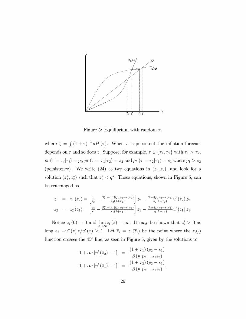
Figure 5: Equilibrium with random τ .

where ζ =R(1 + τ )−1 dH (τ ). When τ is persistent the inflation forecast

depends on τ and so does z. Suppose, for example, τ ∈ τ 1, τ 2 with τ 1 > τ2,

pr (τ = τ i|τ i) = pi, pr (τ = τ1|τ 2) = s2 and pr (τ = τ 2|τ 1) = s1 where p1 > s2

(persistence). We write (24) as two equations in (z1, z2), and look for a

solution (z∗1 , z∗2) such that z

∗i < q∗. These equations, shown in Figure 5, can

be rearranged as

z1 = z1 (z2) =hp1s2− β(1−ασ)(p1p2−s1s2)

s2(1+τ2)

iz2 − βασ(p1p2−s1s2)

s2(1+τ2)u0 (z2) z2

z2 = z2 (z1) =hp2s1− β(1−ασ)(p1p2−s1s2)

s1(1+τ1)

iz1 − βασ(p1p2−s1s2)

s1(1+τ1)u0 (z1) z1.

Notice zi (0) = 0 and limz→∞

zi (z) = ∞. It may be shown that z0i > 0 as

long as −u00 (z) z/u0 (z) ≥ 1. Let zi = zi (zi) be the point where the zi(·)function crosses the 45o line, as seen in Figure 5, given by the solutions to

1 + ασ [u0 (z2)− 1] = (1 + τ 1) (p2 − s1)

β (p1p2 − s1s2)

1 + ασ [u0 (z1)− 1] = (1 + τ 2) (p2 − s1)

β (p1p2 − s1s2).

26

These imply z2 < z1 if τ1 > τ2, and given z0i > 0 this implies z∗1 < z∗2 . Hence,

when the shocks to the money supply are persistent, real balances are smaller

in periods of high inflation, simply because in these periods beliefs about

future inflation are higher.24 It may be interesting to purse these models

with uncertainty, but in what follows we return to deterministic models and

consider the welfare cost of perfectly predictable inflation.

6 Quantitative Analysis

The preference structure used above is U(x, h,X,H) = u(x)−c(h)+U(X)−AH. We specialize things for the quantitative work as follows. First,

u(q) =(q + b)1−η − b1−η

1− η,

where η > 0 and b ∈ (0, 1). This generalizes the standard constant rel-ative risk aversion preferences by including the parameter b, which forces

u(0) = 0.25 We will actually set b ≈ 0 below to make this close to the usualpreferences; hence q∗ = 1− b ≈ 1. Next, U(X) = B log(X); therefore prefer-

ences over centralized market goods here are exactly the same as Cooley and

Hansen (1989), B log(X)− AH. Finally, to make the disutility of labor the

same in the two markets we set c(h) = Ah, and normalize A = 1 (we could

calibrate A to match total hours worked in the data but this affects none of

the welfare calculations). Notice A = 1 implies X∗ = B.

24One detail remains: recall that the equilibrium was constructed conjecturing z∗i < q∗.Since z∗i < z1, for the conjecture to be correct it is sufficient to ensure z1 ≤ q∗, whichholds iff (1 + τ2) (p1 − s2) ≥ β (p1p2 − s1s2).25We require u(0) = 0 because we want the utility of consuming q = 0 to be the same

as the utility of not consuming; this is relevant here because each period agents get toconsume day goods with probability less than 1. We assume b ∈ (0, 1) to guaranteeu0(q) > 0 and q∗ > 0.

27

The period length can basically be anything, but we begin with a year

mainly to facilitate comparison with Lucas (2000); below we show a monthly

model yields very similar results. Hence, we set r = 0.04 for now. In terms

of arrival rates, we can normalize α = 1 since it is only the products αδ

and ασ that matter. We set δ = 0 since barter is relatively rare (this does

not matter for the results). For σ, one might think it can be calibrated to

match velocity ν, but theory does not pin down how much cash is used in

the centralized market.26 Hence, we again follow Lucas and set σ as well

as the preference parameters to match the “money demand” data–that is,

the relationship between the nominal interest rate i and L =M/PY = 1/ν.

This relationship represents “money demand” in the sense that desired real

balances M/P are proportional to Y , with a factor of proportionality L that

depends on the cost of holding cash i.

In the model, nominal output in the centralized market is X∗/φ = B/φ

and nominal output in the decentralized market is σM . Hence PY = B/φ+

σM and Y = B + σφM . In equilibrium, Y = B + σz(q) and

L =M/P

Y=

z(q)

B + σz(q).

Moreover, in steady state

u0(q)z0(q)

= 1 +1− β + τ

σβ= 1 +

i

σ,

and after performing the usual substitutions, β = 1/(1+r) and (1+r)(1+τ) =

26Given their budget constraints, agents are indifferent between receiving wages in termsof general goods or dollars in the night market, since both can be used within the subperiod.If one assumes dollars are used at night only for trades to adjust m velocity is ν = 2σ(because each dollar turns over once in every single-coincidence meeting during the dayand once more at night). At the opposite extreme, if one assumes cash is used in everytransaction in the centralized market, then ν = PY/M , where Y is real output aggregatedacross markets and P the nominal price level.

28

1 + i. This implies q = q(i) , and therefore

L =z[q(i)]

B + σz[q(i)]= L(i). (25)

This is our “money demand” curve: L(i) =M/PY .

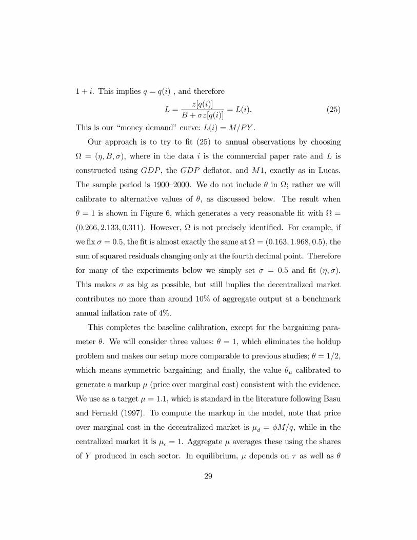
Our approach is to try to fit (25) to annual observations by choosing

Ω = (η,B, σ), where in the data i is the commercial paper rate and L is

constructed using GDP , the GDP deflator, and M1, exactly as in Lucas.

The sample period is 1900—2000. We do not include θ in Ω; rather we will

calibrate to alternative values of θ, as discussed below. The result when

θ = 1 is shown in Figure 6, which generates a very reasonable fit with Ω =

(0.266, 2.133, 0.311). However, Ω is not precisely identified. For example, if

we fix σ = 0.5, the fit is almost exactly the same atΩ = (0.163, 1.968, 0.5), the

sum of squared residuals changing only at the fourth decimal point. Therefore

for many of the experiments below we simply set σ = 0.5 and fit (η, σ).

This makes σ as big as possible, but still implies the decentralized market

contributes no more than around 10% of aggregate output at a benchmark

annual inflation rate of 4%.

This completes the baseline calibration, except for the bargaining para-

meter θ. We will consider three values: θ = 1, which eliminates the holdup

problem and makes our setup more comparable to previous studies; θ = 1/2,

which means symmetric bargaining; and finally, the value θµ calibrated to

generate a markup µ (price over marginal cost) consistent with the evidence.

We use as a target µ = 1.1, which is standard in the literature following Basu

and Fernald (1997). To compute the markup in the model, note that price

over marginal cost in the decentralized market is µd = φM/q, while in the

centralized market it is µc = 1. Aggregate µ averages these using the shares

of Y produced in each sector. In equilibrium, µ depends on τ as well as θ

29

Figure 6: The “money demand” data and fitted L(i).

and Ω. We fit Ω and θ to the data, subject to the constraint µ = 1.1, at the

benchmark inflation rate of 4%. In what follows, then, we consider θ = 1,

1/2, and θµ.

As is standard, our measure of the welfare cost of inflation asks how much

agents would be willing to give up in terms of consumption to have inflation

0 instead of τ . In steady state, for any τ , write utility as

(1− β)V (τ ) = U(X∗)−X∗ + ασ u[qs(τ)]− qs(τ) .

Suppose we reduce τ to 0 but also reduce consumption of both general and

special goods by a factor ∆, so that utility becomes

(1− β)V∆(0) = U(X∗∆)−X∗ + ασ u[qs(0)∆]− qs(0) . (26)

We measure the welfare cost of τ as the value of ∆0 that solves V∆(0) = V (τ );

agents would give up 1 −∆0 percent of consumption to have 0 rather than

τ . We also consider ∆F , which is how much they would give up to have the

Friedman Rule τF rather than τ . Our experiments below use τ = 0.1 (i.e.,

30

we consider the welfare cost of a 10% inflation) but we also report the welfare

costs of inflation rates ranging from 0 to 200% at the end of the section.

In Table 1, the first column of results is for θ = 1 and the fitted Ω, while

the second column of results keeps θ = 1, fixes σ = 0.5 and refits (η,B). As

one can see, the welfare costs of inflation are the same, 1−∆0 = 0.014 and

1 − ∆F = 0.016 (although the equilibrium q is slightly different, as is the

ratio of Y at τ = 0.1 to Y at τ = 0 and the share of the decentralized sector

sd). Since it makes little difference for the welfare results, for the rest of the

experiments in Table 1 we fix σ = 0.5 and fit only (η,B). In any case, the

numbers for our welfare cost in the case θ = 1 are very similar to, if perhaps

slightly bigger than, the typical estimates in the literature–including Lucas

(2000), who actually gives a range of numbers depending on some details,

but reports the typical result for 1−∆0 as just under 1%. We interpret our

results with θ = 1 as being basically consistent with the consensus view in

the literature.27

27To consider some other studies, in Cooley and Hansen (1989) 1−∆F = 0.0015 whenthe cash-in-advance constraint is monthly and 1 −∆F = 0.0052 when it is quarterly. InCooley and Hansen (1991), with cash and credit goods, 1−∆F = 0.0038; by adding taxesthey get it up to 1−∆F = 0.0096. Gomme (1993) finds somewhat lower numbers in anendogenous growth model. Wu and Zhang (2000) argue that the welfare cost of inflation islarger due to monopolistic competition, and provide some more references to other studies.The point here is simply that we are in the same ballpark as most of the literature whenwe set θ = 1.

31

Table 1: Annual Model (1900—2000)r = 0.04 θ = 1 θ = 1 θ = 0.5 θµ = 0.343 θ = 1

Ωσ = 0.31η = 0.27B = 2.13

σ = 0.50η = 0.16B = 1.97

σ = 0.50η = 0.30B = 1.91

σ = 0.50η = 0.39B = 1.78

σ = 0.50η = 0.39B = 1.78

µ (.1)− 1 0.000 0.000 0.031 0.079 0.000µd (.1)− 1 0.000 0.000 0.559 1.352 0.000sd (.1) 0.034 0.050 0.055 0.058 0.128q(τ ) 0.243 0.206 0.143 0.094 0.522q(0) 0.638 0.618 0.442 0.296 0.821q(τF ) 1.000 1.000 0.779 0.568 1.000Y (τ)Y (0)

0.947 0.909 0.914 0.918 0.932

1−∆0 0.014 0.014 0.032 0.046 0.0121−∆F 0.016 0.016 0.041 0.068 0.013

The third column of results in Table 1 now sets θ = 0.5, and refits (η,B).

The fit does not suffer as a result of changing θ (the new curve lies essen-

tially on top of the old one in Figure 6). However, the welfare costs go up

considerably: 1 − ∆0 = 0.032 and 1 − ∆F = 0.041. As one can see, q is

considerably below q∗ at τ = 0.1, and even at τ = 0 or τ = τF . This says the

holdup problem is serious and this is what generates a relatively large cost

of inflation. For this parameterization the aggregate markup is µ = 1.04,

which comes from a markup in the decentralized market of µd = 1.44. The

fourth column reports results with θµ set to generate µ = 1.10, again refitting

(η,B). Now the costs are 1 − ∆0 = 0.046 and 1 − ∆F = 0.068. To verify

that it is the holdup problem that lies at the heart of these effects, the last

column uses the same Ω as the fourth column but sets θ = 1. This yields

costs even lower than in the first two columns. Hence, it is θ < 1 and not

the other parameters that generates the big welfare costs.

32

Table 2: Annual Model (1959—2000)r = 0.04 θ = 1 θ = 0.5 θµ = 0.404 θ = 1

Ωσ = 0.50η = 0.27B = 3.19

σ = 0.50η = 0.45B = 2.92

σ = 0.50η = 0.48B = 2.71

σ = 0.50η = 0.48B = 2.71

µ (.1)− 1 0.000 0.054 0.084 0.000µd (.1)− 1 0.000 0.910 1.451 0.000sd (.1) 0.058 0.059 0.058 0.098q(τ) 0.392 0.192 0.135 0.590q(0) 0.752 0.409 0.307 0.852q(τF ) 1.000 0.602 0.478 1.000Y (τ)Y (0)

0.949 0.950 0.949 0.958

1−∆0 0.008 0.025 0.031 0.0071−∆F 0.009 0.035 0.046 0.008

Table 2 reports similar experiments fitting the model to a shorter sample.

In each case we fix σ = 0.5 and fit (η,B). The qualitative conclusions are

similar to what we found with the longer sample. First, with θ = 1 the

cost of inflation is even lower than shown in Table 1, and thus even more

in line with the literature, coming in at just under 1%. Second, decreasing

θ to 0.5 or to the θµ that generates µ = 1.1 and then refitting (η,B), we

increase the costs considerably; e.g., given θµ, going from τ = 0.1 to 0 is now

worth 3.1% of consumption, and going all the way to τF is now worth 4.6%.

While smaller than the analogous numbers in Table 1, these are still big.

It is interesting (if perhaps not surprising) that the more recent data gives

different “money demand” parameters and a different welfare cost, but what

we want to emphasize here is that regardless of the sample period, going from

θ = 1 to θ < 1 can substantially increase the estimated cost of inflation. And

again, the final column makes it clear that it is the value of θ, and not the

values of (η,B), that is the key to the results.

33

Table 3: Monthly Model (1900—2000)r = 0.04 θ = 1 θ = 0.5 θµ = 0.315 θ = 1

Ωσ = 0.033η = 0.20B = 0.17

σ = 0.052η = 0.23B = 0.15

σ = 0.052η = 0.33B = 0.14

σ = 0.052η = 0.33B = 0.14

µ (.1)− 1 0.000 0.027 0.080 0.000µd (.1)− 1 0.000 0.395 1.101 0.000sd (.1) 0.043 0.068 0.073 0.17q(τ ) 0.230 0.151 0.101 0.552q(0) 0.623 0.476 0.329 0.831q(τF ) 1.000 0.845 0.644 1.000Y (τ)Y (0)

0.932 0.890 0.894 0.921

1−∆0 0.013 0.030 0.049 0.0101−∆F 0.015 0.038 0.069 0.011

In Table 3 we recalibrate so that the period is 1 month–i.e., we simply

transform Y and i in the data to make them monthly. The first column again

fits Ω with θ = 1. Notice that, naturally, the estimated σ and B are lower

in the monthly model, but the overall fit with the “money demand” data

is about the same. In any case, what we really want to emphasize is that

the costs of inflation are almost identical to those in the first two columns of

Table 1. The second column in Table 3 uses θ = 0.5 while the third column

uses θµ, and again the results are almost identical to those in the analogous

cases in Table 1. So the basic conclusion is robust to changing period length

as well as the sample.

Finally, Figure 7 shows the welfare cost 1−∆0 for inflation rates ranging

from 0 to 150%; as is clear from the figure the cost basically converges by

τ = 1.5 since decentralized trade has all but shut down at this point. The

upper curve is for θµ and the implied Ω from the fourth column of Table 1,

while the lower curve is for θ = 1 and the same Ω. The difference in the

34

Figure 7: Welfare costs of large inflations.

curves is due to the holdup problem. Notice that the difference gets smaller

at big inflation rates, because q gets very small for big τ regardless of θ.

Hence, the real difference between models with θ = 1 and θ < 1 is for small

to moderate inflation rates.

7 Conclusion

This paper has presented a new framework for monetary theory and policy

analysis. It is based explicitly on the frictions that make money essential in

the search literature, but without the extreme restrictions usually made in

those models about individuals’ money holdings. The key innovation here

is to allow agents to interact periodically in decentralized and centralized

markets. Given this, if agents have quasi-linear preferences over the good

traded in the centralized market the distribution of money holdings will be

degenerate in equilibrium. This makes the model very tractable. Once we

have a tractable model it is easy to use it to ask many interesting questions.

35

We characterized equilibria and discussed some policy issues. The Fried-

man Rule is optimal, but for bargaining power below 1 it does not achieve

the first best. This can have important quantitative implications for the wel-

fare cost of inflation, as we showed in a calibrated version of the model. It is

not hard to generate welfare costs equivalent to 3% or 5% of consumption–

much bigger than most existing estimates. We also showed how to extend

the model to allow uncertainty in real or monetary variables. We think all

of this constitutes progress in terms of bringing micro and macro models

of monetary economics closer together. We also think that we have only

scratched the surface, and much more could be done in terms of applications

and extensions in future research.

36

A Appendix

In this Appendix we first verify that the bargaining solutions are as claimed in

the text. We then use these results to derive, without using value function V ,

certain properties any equilibrium must satisfy. We then use these properties

to establish the existence and uniqueness of V . Finally, we provide some

details for the proof of Proposition 1.

Lemma 1 In a double coincidence meeting each agent produces q∗ and no

money changes hands.

Proof. The symmetric Nash problem is

maxq1,q2,∆

[u (q1)− c (q2)− φ∆] [u (q2)− c (q1) + φ∆]

subject to −m2 ≤ ∆ ≤ m1, where q1 and q2 denote the quantities consumed

by agents 1 and 2 and ∆ is the amount of money 1 pays 2. There is a unique

solution, characterized by the first order conditions

u0 (q1) [u (q2)− c (q1) + φ∆] = c0 (q1) [u (q1)− c (q2)− φ∆]

c0 (q2) [u (q2)− c (q1) + φ∆] = u0 (q2) [u (q1)− c (q2)− φ∆]

u (q1)− u (q2) + c (q1)− c (q2)− 2φ∆ = (2/φ)(λ1−λ2)[u(q1)−c(q2)−φ∆][u(q2)−c(q1)+φ∆]−1/2

where λi is the multiplier on agent i’s cash constraint. It is easy to see that

q1 = q2 = q∗ and ∆ = λ1 = λ2 = 0 solves these conditions.

Lemma 2 In a single coincidence meeting the bargaining solution is given

by (6).

37

Proof. The necessary and sufficient conditions for (5) are

θ [φd− c (q)] u0 (q) = (1− θ) [u (q)− φd] c0 (q) (27)

θ [φd− c (q)]φ = (1− θ) [u (q)− φd]φ (28)

−λ [u (q)− φd]1−θ [φd− c (q)]θ

where λ is the Lagrange multiplier on d ≤ m. There are two possible cases:

If the constraint does not bind, then λ = 0, q = q∗ and d = m∗. If the

constraint binds then q is given by (27) with d = m, which is (7).

We now present some arbitrage-style arguments to establish that any

equilibrium must satisfy certain conditions. These arguments do not use any

properties of V or F .

Lemma 3 In any equilibrium, βφt+1 ≤ φt for all t.

Proof. First, note that lifetime utility is finite in any equilibrium. Now

suppose by way of contradiction that βφt+1 > φt at some t. In this case,

an agent could raise his production of Yt by dY and sell it for dY/φ dollars,

then use the money at t + 1 to reduce Yt+1 by dY/φt+1 without changing

anything else in his lifetime. Since utility is linear in Y , the net gain from

this is dY (−1+βφt+1/φt) > 0. Hence βφt+1 > φt cannot hold in equilibrium.

Lemma 4 In any equilibrium, mt+1 < m∗t+1 for all t and for all agents.

Proof. Suppose mt+1 > m∗t+1 for some t and some agent. At t he can

change Yt by dY < 0 and carry dmt+1 = dY/φt fewer dollars into t + 1.

Given mt+1 > m∗t+1, for small dY , the bargaining solution says this does not

affect his payoff in the decentralized market. Hence, he can increase Yt+1 by

38

dYt+1 = −dY φt+1/φt and not change anything else in his lifetime, for a netutility gain of dY (1−βφt+1/φt) > 0 by Lemma 3. This proves mt+1 ≤ m∗

t+1.

To establish the strict inequality, assume mt+1 = m∗t+1. Again change Yt

by dY < 0 and carry dmt+1 = dY/φt fewer dollars into t + 1. If he buys in

the decentralized market next period he gets a smaller q but the continuation

value is the same from then on (he still spends all his money). If he is not

a buyer then he can increase Yt+1 by dYt+1 = −dY φt+1/φt and not changeanything else in his lifetime. The net expected utility gain from this is

D = −dY + β£ασu0(qt+1)bq0(mt+1) + (1− ασ)φt+1

¤dY/φt

= −dY (φt − βφt+1)/φt + βασ£u0(qt+1)bq0(mt+1)− φt+1

¤dY/φt.

The first term on the right-hand side is positive by Lemma 3, and the second

is positive for small dY because then mt+1 is near m∗t+1 and this impliesbq0(mt+1) < φt+1/u

0(qt+1) from (8).

Lemma 5 If θ ≈ 1 or u0 is log concave then F is degenerate in any monetaryequilibrium: all agents havemt+1 =M . Given F is degenerate, φt = G

¡φt+1

¢for all t where G is a time-invariant continuous function.

Proof. Consider the following sequence problem: given any path φt, Ftand m0,

maxmt+1∞t=0

∞Xt=0

βt [v (mt, φt, Ft) + φt (mt −mt+1)]

where v is defined in (10) (which does not use V and is defined in terms date

t variables only). We know v is Cn−1; thus, if a solution exists it satisfies the

necessary conditions

βv1¡mt+1, φt+1, Ft+1

¢+ βφt+1 − φt ≤ 0, = 0 if mt+1 > 0. (29)

39

We have v1(m,φ,F ) = ασ [u0(q)bq0(m)− φ], since we know m < m∗, wherebq0(m) is given in (8).In any (monetary) equilibrium, at least one agent must choose mt+1 > 0,

and for this agent

βv1¡mt+1, φt+1, Ft+1

¢+ βφt+1 − φt = 0. (30)

A quick calculation verifies that if θ ≈ 1 or u0 is log concave then v11 < 0,

which implies (30) has a unique solution: all agents choose the same mt+1 =

M . Hence Ft+1 is degenerate in any monetary equilibrium. Finally, (30)

implies φt = G¡φt+1

¢, where G is continuous because v1 is.

We have established F degenerate in any equilibrium, without using dy-

namic programming. This is a step towards constructing a simple proof that

V exists. However, at this point an issue arises: although we know in any

equilibrium that φt = G¡φt+1

¢, for dynamic programming purposes we would

like to know φt+1 = Φ (φt), and G may not be invertible. Our strategy is to

restrict attention to equilibria where φt+1 = Φ (φt) and Φ is continuous. Ob-

viously this includes all steady state equilibria, all possible equilibria in the

case where G is invertible, and many other dynamic equilibria, but it does

not include all possibilities. First note that any equilibrium involves selecting

an initial price φ0, or equivalently q0 since we can invert φ0 = φ(q0) by (7),

and then selecting future values from the correspondence φt+1 = G−1(φt).

We impose only that the selection φt+1 from G−1(φt) cannot vary with time

or the value of φt.

That is, while the value φt+1 obviously varies with φt, the rule for choosing

which branch of G−1 from which to select φt+1 is assumed to be constant. We

know that this is possible for a large class of dynamic equilibria; e.g., one can

always use the rule “select the lowest branch of G−1” and construct equilibria

40

where φt → 0 from any initial φ0 in some interval (0, φ0). While we may not

pick up all possible equilibria given our restriction, we pick up a lot. And

we emphasize that the purpose of this restriction is limited: we already know

that βφt+1 ≤ φt for all t and that F is degenerate in any equilibrium; all we

are doing here is trying to guarantee φt+1 = Φ (φt) where Φ is continuous in

order to prove the existence of the value function V in order to use dynamic

programming (and for steady states, there is no problem).

In any case, even given φt+1 = Φ (φt) where Φ is continuous, we still need

to bound φ. We do this with M constant, but the arguments are basically

the same when M is varying over time if we work with real balances.

Lemma 6 Assume supU(X) > V ≡ u(q∗)+U(X∗)1−β . Then in any equilibrium

φ is bounded above by φ = z/M , where U(z) = V .

Proof. Clearly lifetime utility V in any equilibrium is bounded by V . Con-

sider a candidate equilibrium with φM > z at some date. In the candidate

equilibrium, an individual with m = M would want to deviate by trading

all his money for general goods since U (φM) > V . Hence, φM is bounded

above by z.

Now we can we verify the existence and uniqueness of the value function.

Lemma 7 Let S = R× £0, φ¤ with φ defined as in Lemma 6, and consider

the metric space given by C = v : S→R | v is bounded and continuoustogether with the sup norm, kvk = sup |v (m,φ)|. Define

C0 =nV : S→R|V (m,φ) = v (m,φ) + φm for some v ∈ C

o.

41

Let Φ :£0, φ¤ → £

0, φ¤be a continuous function, and define the operator

T : C0 → C0 by³T V´(m,φ) = sup

m+1

nv (m,φ) + φm− φm+1 + βV [m+1,Φ (φ)]

owhere v(m,φ) is defined in (10). Then T has a unique fixed point V ∈ C0.

Proof. First we show T : C0 → C0. For every V ∈ C0 we can write³T V´(m,φ) = v (m,φ) + φm+ sup

m+1

w [m+1,Φ (φ)]

where w [m+1,Φ (φ)] = βv [m+1,Φ (φ)] + βφm+1 − φm+1 for some v ∈ C.Since v is bounded, there exists a m such that βw[0,Φ (φ)] > βw [m+1,Φ (φ)]

for all m+1 ≥ m. Therefore,

supm+1

w [m+1,Φ (φ)] = maxm+1∈[0,m]

w [m+1,Φ (φ)] ,

and the maximum is attained. Using w∗ (φ) to denote the solution, we have

T V (m,φ) = v (m,φ) + w∗ (φ) + φm ∈ C0, since w∗ (φ) ∈ C by the Theoremof the Maximum and v (x, φ) ∈ C from the bargaining solution.

We now show T is a contraction mapping. Define the norm°°°V1 − V2

°°° =sup |v1 (m,φ)− v2(m,φ)| and consider the metric space (C0, k·k). Fix (m,φ) ∈S. Letting mi

+1 = argmaxm+1∈[0,m]

nβVi [m+1,Φ (φ)]− φm+1

o, we have

T V1 − T V2 =nβV1

£m1+1,Φ (φ)

¤− φm1+1

o−nβV2

£m2+1,Φ (φ)

¤− φm2+1

o≤ β

¯V1£m1+1,Φ (φ)

¤− V2£m1+1,Φ (φ)

¤¯ ≤ β°°°V1 − V2

°°° .Similarly, T V2 − T V1 ≤ β

°°°V1 − V2

°°°. Hence ¯TV2 − T V1

¯≤ β

°°°V1 − V2

°°°.Taking the supremum over (m,φ) we have

°°°TV1 − TV2

°°° ≤ β°°°V1 − V2

°°°, andT satisfies the definition of a contraction.

42

We now argue that (C0, ρ) is complete. Clearly, if Vn(m,φ) = vn(m,φ) +

φm is a Cauchy sequence in C0 then vn(m,φ) is a Cauchy sequence in C.Since (C, k·k) is complete (see, e.g., Stokey and Lucas [1989], Theorem 3.1),

vn → v ∈ C. If we set V = v + φm it is immediate that Vn → V ∈ C0.Therefore (C0, ρ) is complete. It now follows from the Contraction Mapping

Theorem (see, e.g., Stokey and Lucas [1989], Theorem 3.2) that T has a

unique fixed point V ∈ C0.

The final thing to do is fill in some details for the proof of Proposition 1.

Proof of Proposition 1: Most of what is stated follows directly from the

analysis in the text, but two details need to be addressed. First, consider

the uniqueness of the solution to e(q) = 1 + 1−βασβ

for a general θ. This would

follow if e0(0) < 0. Given the normalization c(q) = q,

e(q) =(θu0 + 1− θ)2u0

(θu0 + 1− θ)u0 − θ(1− θ)(u− c)u00.

Therefore e0 takes the same sign as

D1 = [(θu0 + 1− θ)u0 − θ(1− θ)(u− c)u00] [(θu0 + 1− θ)u00 + 2θu0u00]

−u0(θu0 + 1− θ) [(θu0 + 1− θ)u00 + θu0u00]

+u0(θu0 + 1− θ) [θ(1− θ)(u0 − 1)u00 + θ(1− θ)(u− c)u000] .

After simplification we arrive at

D1 = −2θ2(1− θ)(u− c)u0u002 + θ(θu0 + 1− θ) [u0 + (1− θ)(u0 − 1)u0u00]−θ(1− θ)(θu0 + 1− θ)(u− c)u002 + θ(1− θ)(θu0 + 1− θ)(u− c)u0u000.

Since qs < q∗, we have u0 > 1 and all but the final term are unambiguously

negative. If θ = 1 this term vanishes and D1 < 0. For any θ ∈ (0, 1), if u0 is

43

log-concave then u0u000 < u00, and this term is bounded by the previous term

and so again we have D1 < 0.

Second, we show that e shifts up with an increase in θ at the solution to

e(q) = 1 + 1−βασβ. To begin, note that ∂e/∂θ takes the same sign as

D2 = 2(u0 − 1) [(θu0 + 1− θ)u0 − θ(1− θ)(u− c)u00]

−(θu0 + 1− θ) [u0(u0 − 1)− (1− 2θ)(u− c)u00]

= (θu0 + 1− θ)(u0 − 1)u0 − (θu0 − 1 + θ)(u− c)u00

Now rearrange e(q) = 1 + 1−βασβ

as

(u− c)u00 =(θu0 + 1− θ)u0

θ(1− θ)³1 + 1−β

ασβ

´ µ1− β

ασβ+ θ − θu0

¶

Substituting this into D2 and simplifying, at e(q) = 1 +1−βασβ

we see that D2

takes the same sign as 1−βασβ(1− θ)2 + θ2u0(u0 − e). The desired result follows

if we can show u0 ≥ e, which is easy to establish.

44

References

[1] Aiyagari, S. Rao, and Neil Wallace. “Existence of Steady States withPositive Consumption in the Kiyotaki-Wright Model.” Review of Eco-nomic Studies 58(5) (October 1991): 901—916.

[2] Alvarez, Fernando, and Nancy L. Stokey. “Dynamic Programming withHomogeneous Functions.” Journal of Economic Theory 82(1) (Septem-ber 1998): 167—189.

[3] Aruoba, S. Boragan and Randall Wright. “Search, Money, and Capital:A Neoclassical Dichotomy.” Unpublished manuscript, Federal ReserveBank of Cleveland, 2002.

[4] Basu, Susanto and Fernald, John. “Returns to scale in U.S. production:Estimates and implications,” Journal of Political Economy 105(2) (April1997): 249—283.

[5] Berentsen, Aleksander. “On the Distribution of Money Holdings in aRandom-Matching Model.” International Economic Review 43(3) (Au-gust 2002): 945—954.

[6] Berentsen, Aleksander, and Guillaume Rocheteau. “Money and theGains from Trade.” International Economic Review 44(1) (February2003): 263—297.

[7] Berentsen, Aleksander, and Guillaume Rocheteau. “On the Efficiencyof Monetary Exchange: How Divisibility of Money Matters.” Journal ofMonetary Economics 49(8) (November 2002): 1621—1649.

[8] Berentsen, Aleksander, and Guillaume Rocheteau. “On the FriedmanRule in Search Models with Divisible Money.” Contributions to Macro-economics 3(1) 2003.

[9] Berentsen, Aleksander, Guillaume Rocheteau and Shouyong Shi. “Fried-man Meets Hosios: Efficiency in Search Models of Money.” Unpublishedmanuscript, 2001.

[10] Camera, Gabriele, and Dean Corbae. “Money and Price Dispersion.”International Economic Review 40(4) (November 1999): 985—1008.

45

[11] Christiano, Lawrence, Martin Eichenbaum. “Current Real-Business-Cycle Theories and Aggregate Labor-Market Fluctuations,” AmericanEconomic Review 82(3) (June 1992): 430—450.

[12] Christiano, Lawrence, Martin Eichenbaum and Charles Evans. “StickyPrice and Limited ParticipationModels: A Comparison,” European Eco-nomic Review 41(6) (June 1997): 1201—1249.

[13] Cooley, Thomas and Gary Hansen. “The Inflation Tax in a Real Busi-ness Cycle Model.”American Economic Review 79(4) (September 1989):733—748.

[14] Cooley, Thomas and Gary Hansen. “The Welfare Costs of ModerateInflations.” Journal of Money, Credit and Banking 23(3) (August 1991,Part 2): 483—503.

[15] Duffie, Darrell, John Geanakoplos, Andreu Mas-Colell and AndrewMcLennan. “Stationary Markov Equilibria.” Econometrica 62(4) (July1994): 745—781.

[16] Faig, Miguel. “A Search Theory of Money with Commerce and Neoclas-sical Production.” Unpublished manuscript, 2001.

[17] Friedman, Milton. The Optimal Quantity of Money and Other Essays.Chicago: Adeline, 1969.

[18] Gomme, Paul. “Money and Growth Revisited: Measuring the Cost ofInflation in an Endogenous Growth Model.” Journal of Monetary Eco-nomics 32(1) (August 1993): 51—77.

[19] Green, Edward, and Ruilin Zhou. “A Rudimentary Random-MatchingModel with Divisible Money and Prices.” Journal of Economic Theory81(2) (August 1998): 252—271.

[20] Hansen, Gary D. “Indivisible Labor and the Business Cycle,” Journalof Monetary Economics 16(3) (November 1985): 309—327.

[21] Head, Allen and Alok Kumar. “Price-posting, price dispersion, and in-flation in a random matching model.” International Economic Review(2005), in press.

46

[22] Hosios, Arthur J. “On the Efficiency of Matching and Related Models ofSearch and Unemployment.” Review of Economic Studies 57(2) (April1990): 279—298.

[23] Khan, Aubhik, Julia K. Thomas, and Randall Wright. “Money and Dis-tribution: Quantitative Theory and Political Analysis.” Unpublishedmanuscript, University of Pennsylvania, 2003.

[24] Kiyotaki, Nobuhiro and John Moore. “Liquidity, Business Cycles andMonetary Policy.” Lecture 2, Clarendon Lectures, November 2001.

[25] Kiyotaki, Nobuhiro and Randall Wright. “On Money as a Medium ofExchange.” Journal of Political Economy 97(4) (August 1989): 927—954.

[26] Kiyotaki, Nobuhiro and Randall Wright. “A Contribution to the PureTheory of Money.” Journal of Economic Theory 53(2) (April 1991):215—235.

[27] Kiyotaki, Nobuhiro and Randall Wright. “A Search-Theoretic Approachto Monetary Economics.” American Economic Review 83(1) (March1993): 63—77.

[28] Kocherlakota, Narayana. “Money is Memory.” Journal of EconomicTheory 81(2) (August 1998): 232—251.

[29] Lagos, Ricardo and Randall Wright “Dynamics, Cycles and SunspotEquilibria in ‘Genuinely Dynamic, Fundamentally Disaggregative’ Mod-els of Money.” Journal of Economic Theory 109(2) (April 2003): 156—171.

[30] Lagos, Ricardo and Guillaume Rocheteau. “Coexistence of Money andReal Assets.” Unpublished manuscript, 2002.

[31] Lucas, Robert E. Jr. “Inflation and Welfare.” Econometrica 68(2)(March 2000): 247—274.

[32] Lucas, Robert E. Jr. and Nancy Stokey. “Optimal Fiscal and MonetaryPolicy in an Economy without Capital.” Journal of Monetary Economics12(1) (July 1983): 55—93.

47

[33] Lucas, Robert E. Jr. and Nancy Stokey. “Money and Interest in a Cash-in-Advance Economy.” Econometrica 55(3) (May 1987): 491—513.

[34] Molico, Miguel. “The Distribution of Money and Prices in Search Equi-librium.” unpublished manuscript, 1999.

[35] Rauch, Bernard. “A Divisible Search Model of Fiat Money: A Com-ment.” Econometrica 68(1) (January 2000): 149—156.

[36] Rogerson, Richard. “Indivisible Labor, Lotteries and Equilibrium.”Journal of Monetary Economics 21(1) (1988): 3—16.

[37] Shi, Shouyong. “Money and Prices: A Model of Search and Bargaining.”Journal of Economic Theory 67(2) (December 1995): 467—496.

[38] Shi, Shouyong. “A Divisible Search Model of Fiat Money.” Econometrica64(1) (January 1997): 75—102.

[39] Shi, Shouyong. “Search for a Monetary Propagation Mechanism.” Jour-nal of Economic Theory 81(2) (August 1998): 314—352.

[40] Shi, Shouyong. “Search, Inflation and Capital Accumulation.” Journalof Monetary Economics 44(1) (August 1999): 81—103.

[41] Stokey, Nancy and Lucas, Robert E. Jr. Recursive Methods in EconomicDynamics. Cambridge: Harvard University Press, 1989.

[42] Taber, Alexander and Neil Wallace. “A Matching Model with BoundedHoldings of Indivisible Money.” International Economic Review 40(4)(November 1999): 961—984.

[43] Trejos, Alberto and Randall Wright. “Search, Bargaining, Money andPrices.” Journal of Political Economy 103(1) (February 1995): 118—141.

[44] Walsh, Carl E. Monetary Theory and Policy. Cambridge and London:MIT Press, 1998.

[45] Wallace, Neil. “Whither monetary economics?” International EconomicReview 42(4) (November 2001): 847—869.

48

[46] Williamson, Steve and Wright, Randall (2003). “Seasonality and mone-tary policy.” Unpublished manuscript, 2003.

[47] Wu, Yangru and Junxi Zhang. “Monopolistic Competition, IncreasingReturns to Scale and the Welfare Costs of Inflation.” Journal of Mone-tary Economics 46(2) (October 2000): 417—440.

[48] Zhou, Ruilin. “Individual and Aggregate Real Balances in a Random-Matching Model.” International Economic Review 40(4) (November1999): 1009—1038.

49