a unified approach to model selection and sparse recovery ...jinchilv/publications/aos-lf09.pdf ·...

The Annals of Statistics2009, Vol. 37, No. 6A, 3498–3528DOI: 10.1214/09-AOS683© Institute of Mathematical Statistics, 2009

A UNIFIED APPROACH TO MODEL SELECTION AND SPARSERECOVERY USING REGULARIZED LEAST SQUARES1

BY JINCHI LV AND YINGYING FAN

University of Southern California

Model selection and sparse recovery are two important problems forwhich many regularization methods have been proposed. We study the prop-erties of regularization methods in both problems under the unified frame-work of regularized least squares with concave penalties. For model selection,we establish conditions under which a regularized least squares estimator en-joys a nonasymptotic property, called the weak oracle property, where the di-mensionality can grow exponentially with sample size. For sparse recovery,we present a sufficient condition that ensures the recoverability of the spars-est solution. In particular, we approach both problems by considering a familyof penalties that give a smooth homotopy between L0 and L1 penalties. Wealso propose the sequentially and iteratively reweighted squares (SIRS) algo-rithm for sparse recovery. Numerical studies support our theoretical resultsand demonstrate the advantage of our new methods for model selection andsparse recovery.

1. Introduction. Model selection and sparse recovery are two important areasthat have attracted much attention of the researchers. They are different but related,and share some common ideas especially when dealing with large scale problems.Examples include the lasso [Tibshirani (1996)], SCAD [Fan (1997) and Fan andLi (2001)], Dantzig selector [Candes and Tao (2007)] and MCP [Zhang (2007)] inmodel selection, and the basis pursuit [Chen, Donoho and Saunders (1999)] andmany other L1 methods [Candes and Tao (2005, 2006) and Candès, Wakin andBoyd (2008)] in sparse recovery. The analysis of vast data sets with the numberof variables p comparable to or much larger than the number of observations n

frequently arises nowadays in both areas and poses many challenges that are notpresent in smaller scale studies. Sparsity plays an important role in these large scaleproblems. It is often believed that only a small fraction of the data is informative,whereas most of it is noise.

Consider the linear regression model

y = Xβ + ε,(1)

Received February 2008; revised January 2009.1Supported in part by NSF Grants DMS-08-06030 and DMS-09-06784 and 2008 Zumberge Indi-

vidual Award from USC’s James H. Zumberge Faculty Research and Innovation Fund.AMS 2000 subject classifications. Primary 62J99; secondary 62F99.Key words and phrases. Model selection, sparse recovery, high dimensionality, concave penalty,

regularized least squares, weak oracle property.

3498

http://www.imstat.org/aos/

http://dx.doi.org/10.1214/09-AOS683

http://www.imstat.org

http://www.ams.org/msc/

REGULARIZED LEAST SQUARES 3499

where y is an n-dimensional vector of responses, X = (x1, . . . ,xp) is an n × p

design matrix, β = (β1, . . . , βp)T is an unknown p-dimensional vector of re-gression coefficients and ε is an n-dimensional vector of noises. In the sparsemodeling, we assume that a fraction of the true regression coefficients vectorβ0 = (β0,1, . . . , β0,p)T are exactly zero. In this paper we allow β0 to depend on n.We denote by M0 = supp(β0) the support of β0, which is called the true under-lying sparse model hereafter. Model selection aims to locate those predictors xj

with nonzero β0,j , which are called true variables hereafter, and to give consis-tent estimate of β0 on its support. Throughout the paper we consider deterministicdesign matrix X and assume the identifiability of β0, in the sense that the equa-tion Xβ0 = Xβ , β ∈ Rp entails either β = β0 or ‖β‖0 > ‖β0‖0. We denote by‖ · ‖q the Lq norm on the Euclidean spaces q ∈ [0,∞]. Many methods have beenproposed in the literature to construct estimators that mimic the oracle estimatorsunder different losses, where the oracle knew the true model M0 ahead of time.The main difficulty of recovering M0 lies in the collinearity among the predictors,which increases as the dimensionality grows. See, for example, Fan and Li (2006)for a comprehensive overview of challenges of high dimensionality in statistics.

Much insight into model selection can be obtained if we understand a closely re-lated problem of sparse recovery, which aims at finding the minimum L0 (sparsestpossible) solution to the linear equation

y = Xβ,(2)

where β = (β1, . . . , βp)T , y = Xβ0 and X and β0 are the same as those in thelinear model (1). The identifiability of β0 assumed above ensures that our targetsolution here is unique and exactly β0. When the p × p matrix XT X is singular orclose to singular, finding β0 is not an easy task. It is known that directly solvingthe L0-regularization problem is combinatorial and, thus, is impractical in highdimensions. To attenuate this difficulty, many regularization methods such as theL1 method of basis pursuit have been proposed to recover β0, where continuouspenalty functions are used in place of the L0 penalty. This raises a natural ques-tion: under what conditions does a regularization method give the same solution asthat of the L0 regularization? Many authors have contributed to identifying con-ditions that ensure the L1/L0 equivalence. In this paper we generalize a sufficientcondition identified for the L1 penalty to concave penalties, which ensures such anequivalence.

In view of (1) and (2), model selection and sparse recovery can be regarded astwo interrelated problems. Due to the presence of noise, recovering the true modelM0 in (1) is intrinsically more challenging than recovering the sparsest possiblesolution β0 in (2). Various regularization methods in model selection such as thosementioned before have been studied by many researchers. See, for example, Bickeland Li (2006) for a comprehensive review of regularization methods in statistics.

In a seminal paper, Fan and Li (2001) lay down the theoretical foundation ofnonconvex penalized least squares and nonconcave penalized likelihood for vari-able selection, and introduce the concept of model selection oracle property. An

3500 J. LV AND Y. FAN

estimator β is said to have the oracle property [Fan and Li (2001)] if: (1) it en-joys the sparsity in the sense of βMc

0= 0 with probability tending to 1 as n → ∞,

and (2) it attains an information bound mimicking that of the oracle estimator [seealso Donoho and Johnstone (1994)], where βMc

0is a subvector of β formed by

components with indices in Mc0, the complement of the true model M0. Fan and

Li (2001) study the oracle properties of nonconcave penalized likelihood estima-tors in the finite-dimensional setting. Their results were extended later by Fan andPeng (2004) to the setting of p = o(n1/5) or o(n1/3). In this paper we general-ize the results of Fan and Li (2001) and Fan and Peng (2004), in the setting ofregularized least squares, to a more general triple (s, n,p) for concave penalties,where s = ‖β0‖0. In particular, we show that under some regularity conditions, theregularized least squares estimator enjoys a nonasymptotic weak oracle property,where the dimensionality p can be of exponential order in sample size n. Thisconstitutes one of the main contributions of the paper.

In this paper, we consider both problems of model selection and sparse recov-ery in the unified framework of regularized least squares with concave penalties.Specifically, for sparse recovery we construct the solutions of regularization prob-lems under the constraint in (2) by analyzing the solutions of related regularizedleast squares problems and then letting the regularization parameter λ → 0+. Inparticular, we consider a family of penalty functions that give a smooth homotopybetween L0 and L1 penalties for both problems. The unified approach using the L1penalty has been considered by Chen, Donoho and Saunders (1999), Fuchs (2004),Donoho, Elad and Temlyakov (2006) and Tropp (2006), among others.

The rest of the paper is organized as follows. In Section 2, we discuss the choiceof penalty functions. We study the properties of regularization methods in modelselection and sparse recovery for concave penalties in Sections 3 and 4. Section 5discusses algorithms for solving regularization problems. In Section 6 we presentfour numerical examples using both simulated and real data sets. Proofs are pre-sented in Section 7. We provide some discussion of our results and their implica-tions in Section 8.

2. Regularization methods with concave penalties. In this paper, we studyregularization methods in model selection and sparse recovery for concave penal-ties. For sparse recovery in (2), we consider the ρ-regularization problem

minp∑

j=1

ρ(|βj |) subject to y = Xβ,(3)

where ρ(·) is a penalty function and β = (β1, . . . , βp)T . For model selection in (1),we consider the regularized least squares problem

minβ∈Rp

{2−1‖y − Xβ‖2

2 + �n

p∑j=1

pλn(|βj |)},(4)


where �n ∈ (0,∞) is a scale parameter, pλn(·) is a penalty function, λn ∈ [0,∞)

is a regularization parameter indexed by sample size n and β = (β1, . . . , βp)T .We will drop the subscript n when it causes no confusion. For any penalty func-tion pλ, let ρ(t;λ) = λ−1pλ(t) for t ∈ [0,∞) and λ ∈ (0,∞). For simplicity, wewill slightly abuse the notation and write ρ(t;λ) as ρ(t) when there is no confu-sion.

2.1. Penalty functions. By the nature of sparse recovery, the L0 penalty ρ(t) =I (t �= 0) is the target penalty in (3), whereas other penalties may also be capableof recovering β0. As mentioned before, the L0 penalty is not appealing from thecomputational point of view due to its discontinuity. It is known that the L2 penaltyρ(t) = t2 in (3) or (4) is analytically tractable, but generally produces nonsparsesolutions. Such concerns have motivated the use of penalties that are computation-ally tractable approximations or relaxations to the L0 penalty. Among all proposalsthe L1 penalty ρ(t) = t , t ∈ [0,∞), has attracted much attention of the researchersin both sparse recovery and model selection. It has been recognized that the L1penalty is not an oracle that always points us to the true underlying sparse model.

Hereafter, we consider penalty functions ρ(·) that satisfy the following condi-tion.

CONDITION 1. ρ(t) is increasing and concave in t ∈ [0,∞), and has a con-tinuous derivative ρ′(t) with ρ ′(0+) ∈ (0,∞). If ρ(t) is dependent on λ, ρ ′(t;λ)

is increasing in λ ∈ (0,∞) and ρ′(0+) is independent of λ.

Fan and Li (2001) advocate penalty functions that give estimators with threedesired properties—unbiasedness, sparsity and continuity—and provide insightsinto them [see also Antoniadis and Fan (2001)]. We discuss the connection ofCondition 1 with these properties. Consider problem (4) with n × 1 orthonormaldesign matrix and �n = 1,

minθ∈R

{2−1(z − θ)2 + pλ(|θ |)},(5)

where z = XT y and pλ(t) = λρ(t), t ∈ [0,∞). We denote by θ (z) the minimizerof problem (5). Fan and Li (2001) demonstrate that for the resulting estimatorθ (z): (1) unbiasedness requires that the derivative p′

λ(t) is close to zero when t ∈[0,∞) is large, (2) sparsity requires p′

λ(0+) > 0 and (3) continuity with respectto data z requires that the function t + p′

λ(t), t ∈ [0,∞) attains its minimum att = 0. Note that the concavity of ρ in Condition 1 entails that ρ ′(t) is decreasing int ∈ [0,∞). Thus penalties satisfying Condition 1 and limt→∞ ρ′(t) = 0 enjoy theunbiasedness and sparsity. However, the continuity does not generally hold for allpenalties in this class. The SCAD penalty [Fan and Li (2001)] pλ(t), t ∈ [0,∞),is given by

p′λ(t) = λ

{I (t ≤ λ) + (aλ − t)+

(a − 1)λI (t > λ)

}for some a > 2,(6)


where often a = 3.7 is used, and MCP [Zhang (2007)] pλ(t), t ∈ [0,∞), is givenby p′

λ(t) = (aλ − t)+/a. Both SCAD and MCP with a ≥ 1 satisfy Condition 1and the above three properties simultaneously. Although the L1 penalty satisfiesCondition 1 as well as sparsity and continuity, it does not enjoy the unbiasedness,since its derivative is identically one regardless of t ∈ [0,∞).

For a penalty function ρ, we define its maximum concavity as

κ(ρ) = supt1,t2∈(0,∞),t1<t2

−ρ′(t2) − ρ′(t1)t2 − t1

(7)

and we define the local concavity of the penalty ρ at b = (b1, . . . , bq)T ∈ Rq with

‖b‖0 = q as

κ(ρ;b) = limε→0+ max

1≤j≤qsup

t1,t2∈(|bj |−ε,|bj |+ε),t1<t2

−ρ′(t2) − ρ′(t1)t2 − t1

.(8)

By the concavity of ρ in Condition 1, we have 0 ≤ κ(ρ;b) ≤ κ(ρ). It is easy toshow by the mean-value theorem that κ(ρ) defined in (7) equals supt∈(0,∞) −ρ′′(t)and κ(ρ;b) defined in (8) equals max1≤j≤q −ρ′′(|bj |), provided that ρ has a con-tinuous second derivative ρ′′(t).

2.2. A family of penalties. Nikolova (2000) studies the transformed L1 penaltyfunction ρ(t) = bt/(1+bt), t ∈ [0,∞) and b > 0. A slight modification of it givesa family of penalties {ρa :a ∈ [0,∞]} given by, for a ∈ (0,∞),

ρa(t) = (a + 1)t

a + t=

(t

a + t

)I (t �= 0) +

(a

a + t

)t, t ∈ [0,∞),(9)

and

ρ0(t) = lima→0+ρa(t) = I (t �= 0) and ρ∞(t) = lim

a→∞ρa(t) = t(10)

for t ∈ [0,∞). Figure 1 depicts ρa penalties for a few a’s. We see from (9) that thismodified family has the interpretation of a smooth homotopy between L0 and L1penalties. So we refer to them as the smooth integration of counting and absolutedeviation (SICA) penalties. It is easy to show that ρa penalty with a ∈ (0,∞]satisfies Condition 1, and for each a ∈ (0,∞), limt→∞ ρ′

a(t) = 0. Thus ρa witha ∈ (0,∞) gives estimators satisfying the unbiasedness and sparsity. As mentionedbefore, the continuity requires that the function t + λρ′

a(t), t ∈ [0,∞), attains itsminimum at t = 0; that is, a ∈ [a0,∞], where a0 = λ + √

λ2 + 2λ. Therefore, ρa

penalties ρa with a ∈ [a0,∞) satisfy Condition 1 and the above three propertiessimultaneously, and share the same spirit as SCAD and MCP. In addition, ρa isinfinitely differentiable on [0,∞) for each a ∈ (0,∞]. The idea of linearly com-bining L0 and L1 penalties was investigated by Liu and Wu (2007).

For each a ∈ (0,∞), the ρa penalty is closely related to the log penalty

ρ1,a(t) = (a + 1) log(1 + a−1t), t ∈ [0,∞).


FIG. 1. Plot of penalty functions ρ0 (L0, thick solid), ρ0.2 (dash-dot), ρ1 (dashed), ρ5 (dotted),and ρ∞ (L1, thin solid).

In fact, the L1 penalty is the first-order approximation to both a(a +1)−1ρa(t) anda(a + 1)−1ρ1,a(t), and always dominates them. Also, we have ρa(t) = tρ′

1,a(t).Clearly,

ρ′a(t) = a(a + 1)

(a + t)2 , t ∈ (0,∞) for a ∈ (0,∞),

(11)ρ′

a(0+) = 1 + a−1 for a ∈ (0,∞) and ρ′∞(t) = 1.

It is easy to see that the maximum concavity of ρa penalty is

κ(ρa) = supt∈(0,∞)

−ρ′′a (t) = sup

t∈(0,∞)

2a(a + 1)

(a + t)3 = 2(a−1 + a−2),(12)

which is the maximum curvature of the curve ρa . Clearly, κ(ρa) is decreasing in a,lima→0+ κ(ρa) = ∞, and lima→∞ κ(ρa) = 0 = κ(ρ∞). Therefore, parameter a

controls the maximum concavity of ρa and regulates where it stands between L0and L1 penalties.

3. Sparse recovery. In this section we consider the ρ-regularization prob-lem (3) for sparse recovery in (2). It is known that when the n × p matrix X is offull column rank p, (2) has a unique solution β = (XT X)−1XT y. Otherwise, it hasan infinite number of solutions, all of which form a q-dimensional linear subspace

A = {β ∈ Rp : y = Xβ}(13)

of Rp with q = p − rank(X). Of interest is the nontrivial case of q > 0.


3.1. Identifiability of β0. As mentioned in the Introduction, the minimum L0solution to (2) is

β0 = arg minβ∈A

‖β‖0.(14)

Donoho and Elad (2003) introduce the concept of spark and show that the unique-ness of β0 can be characterized by the spark(X) of X, where τ = spark(X) isdefined as the smallest possible number such that there exists a subgroup of τ

columns from the n × p matrix X that are linearly dependent. The spark of a ma-trix can be very different from its rank. For instance, the n × (n + 1) matrix [Ine1]is of full rank n and yet has spark equal to 2, where e1 = (1,0, . . . ,0)T . In partic-ular, they proved that any β ∈ A with ‖β‖0 < spark(X)/2 meets β0. Thus β0 isunique as long as ‖β0‖0 < spark(X)/2.

3.2. L2 penalty. When the ρ penalty is taken to be the L2 penalty in the ρ-regularization problem (3), its minimizer is given by

β2 = arg minβ∈A

‖β‖2.(15)

It admits a closed-form solution. Viewing in the linear regression setting, we knowthat [see Theorem 6.2.1 in Fang and Zhang (1990)] the least squares estimate(XT X)+XT y is a solution to the normal equation XT y = XT Xβ , where (·)+ de-notes the Moore–Penrose generalized matrix inverse. The following propositionshows that it coincides with β2.

PROPOSITION 1 (Minimum L2 solution). β2 = (XT X)+XT y.

However, the minimum L2 solution β2 to (2) is generally nonsparse and, thus,is different from the minimum L0 solution β0.

3.3. Penalties satisfying Condition 1. We are curious about the ρ/L0 equiv-alence, in the sense that the minimizer of the ρ-regularization problem (3) meetsthe minimum L0 solution β0. As mentioned in the Introduction, many researchershave contributed to identifying conditions that ensure the L1/L0 equivalencewhen ρ is taken to be the L1 penalty. We consider penalties ρ satisfying Con-dition 1. It is generally difficult to study the global minimizer analytically withoutconvexity. As is common in the literature, we study the behavior of local minimiz-ers.

Directly studying the local minimizer of the ρ-regularization problem (3) isgenerally difficult. We take the idea of constructing a solution to (3) by analyzingthe solution of related ρ-regularized least squares problem (4) with regularizationparameter λ ∈ (0,∞) and then letting λ → 0+, where pλ(t) = λρ(t), t ∈ [0,∞).

We introduce some notation to simplify our presentation. For any S ⊂ {1,

. . . , p}, XS stands for an n × |S| submatrix of X formed by columns with in-


dices in S, bS stands for the subvector of b formed by components with indicesin S and Sc denotes its complement. For any vector b = (b1, . . . , bq)

T , definesgn(b) = (sgn(b1), . . . , sgn(bq))T , where the sign function sgn(x) = 1 if x > 0,−1 if x < 0 and 0 if x = 0. Let

ρ(t) = sgn(t)ρ ′(|t |), t ∈ R,(16)

and ρ(b) = (ρ(b1), . . . , ρ(bq))T , b = (b1, . . . , bq)T . Clearly, for a ∈ (0,∞),

ρa(t) = sgn(t)a(a + 1)/(a + |t |)2 and ρ∞(t) = sgn(t), t ∈ R,(17)

where ρa is defined in (9) and (10).The following theorem gives a sufficient condition on the strict local minimizer

of (4) for any n-vector y and n × p matrix X.

THEOREM 1 (Regularized least squares). Assume that pλ satisfies Condi-

tion 1 and βλ ∈ Rp with Q = XT

MλXMλ

nonsingular, where λ ∈ (0,∞) and

Mλ = supp(βλ). Then β

λis a strict local minimizer of (4) with λn = λ if

βλ

Mλ= Q−1XT

Mλy − �nλQ−1ρ(β

λ

Mλ),(18)

‖zMcλ‖∞ < ρ′(0+),(19)

λmin(Q) > �nλκ(ρ; βλ

Mλ),(20)

where z = (�nλ)−1XT (y − Xβλ), λmin(·) denotes the smallest eigenvalue of a

given symmetric matrix, and κ(ρ; βλ

Mλ) is given by (8).

Conditions (18) and (20) ensure that βλ

is a strict local minimizer of (4) whenconstrained on the ‖βλ‖0-dimensional subspace {β ∈ Rp :βMc

λ= 0} of Rp . Con-

dition (19) makes sure that the sparse vector βλ

is indeed a strict local minimizerof (4) on the whole space Rp . When ρ is convex, (19) and (20) can be, respec-tively, relaxed to no greater than and no less than under which β

λis a minimizer

of (4). Due to the possible nonconvexity of ρ, the technical analysis for provinglocal minimizer needs the strict inequalities in (19) and (20).

When ρ is taken to be the L1 penalty, the objective function in (4) is con-vex. Then the classical convex optimization theory applies to show that β

λ =(βλ

1 , . . . , βλp) is a global minimizer if and only if there exists a subgradient z ∈

∂L1(βλ), such that

XT Xβλ − XT y + �nλz = 0,(21)

where the subdifferential of the L1 penalty is given by ∂L1(βλ) = {z = (z1, . . . ,

zp)T ∈ Rp : zj = sgn(βλj ) for βλ

j �= 0 and zj ∈ [−1,1] otherwise}. Thus provided

that Q = XTMλ

XMλis nonsingular with Mλ = supp(β

λ), condition (21) reduces to


(18) and (19) with < and ρ′(0+) replaced by ≤ and 1, respectively, whereas bythe nonsingularity of Q, condition (20) always holds for the L1 penalty. However,to ensure that β

λis the strict minimizer we need the strict inequality in (19). These

conditions for the L1 penalty have been extensively studied by many authors, forexample, Efron et al. (2004), Fuchs (2004), Tropp (2006), Wainwright (2006) andZhao and Yu (2006), among others.

By analyzing the solution of (4) characterized by Theorem 1 and letting λ →0+, we obtain the following theorem providing a sufficient condition which en-sures that β0 is a local minimizer of (3).

THEOREM 2 (Sparse recovery). Assume that ρ satisfies Condition 1 withκ(ρ) ∈ [0,∞), Q = XT

M0XM0 is nonsingular with M0 = supp(β0), and X =

(x1, . . . ,xp). Then β0 is a local minimizer of (3) if there exists some ε ∈(0,minj∈M0 |β0,j |) such that

maxj∈Mc

0

maxu∈Uε

|〈xj ,u〉| < ρ′(0+),(22)

where Uε = {XM0Q−1ρ(v) : v ∈ Vε} and Vε = ∏j∈M0

{t : |t − β0,j | ≤ ε}.

We make some remarks on Theorem 2. Clearly condition (22) is free of thescale of the penalty function, that is, invariant under the rescaling ρ → cρ forany constant c ∈ (0,∞). Condition (22) is independent of the scale of X, anddepends on β0 through M0 and a small neighborhood Vε of β0,M0

. It can beviewed as a local condition at (M0,β0,M0

). For the L1 penalty ρ∞, we haveρ′∞(0+) = 1 and for any ε ∈ (0,minj∈M0 |β0,j |), Uε contains a single pointu0 = XM0Q−1 sgn(β0,M0

). This shows that for the L1 penalty, condition (22) re-duces to the following condition

maxj∈Mc

0

|〈xj ,u0〉| < 1,(23)

which can actually be relaxed to maxj∈Mc0|〈xj ,u0〉| ≤ 1 while ensuring the L1/L0

equivalence. In the context of model selection, condition (23) was called the weakirrepresentable condition in Zhao and Yu (2006), who introduced it for character-izing the selection consistency of lasso. For the ρa penalty with a ∈ (0,∞), by(11) we have

ρ′a(0+) = 1 + a−1 → ∞ and ρ′

a(t) = a(a + 1)

(a + t)2 → 0 as a → 0+for each t ∈ (0,∞), which shows that condition (22) is less restrictive forsmaller a. This justifies the flexibility of the ρa penalties.

A great deal of research has contributed to identifying conditions on X and β0that ensure the L1/L0 equivalence. See, for example, Chen, Donoho and Saun-ders (1999), Donoho and Elad (2003), Donoho (2004) and Candes and Tao (2005,


2006). In particular, Donoho (2004) shows that the individual equivalence ofL1/L0 depends only on M0 and β0,M0

. Condition (23) is independent of the scaleof X, and depends on β0 only through M0 and β0,M0

, sharing the same spirit. Theidea of using weighted L1 penalty in the ρ-regularization problem (3) has beenproposed and studied by Candès, Wakin and Boyd (2008).

3.4. Optimal ρa penalty. Theorem 2 gives one characterization of the role ofpenalty functions in sparse recovery (2). In this section, we identify the optimalpenalty ρa for given X and β0 in sparse recovery.

For any ε ∈ (0,minj∈M0 |β0,j |), we define

Pε = {All penalties ρa in (3) that satisfy condition (22)}.(24)

By Theorem 2, any ρa penalty in Pε ensures that β0 is recoverable in theory bythe ρa-regularization problem (3). We are interested in a penalty ρaopt(ε) that attainsthe minimal maximum concavity in the sense that

κ(ρaopt(ε)

) = infρa∈Pε

κ(ρa).(25)

Such penalty ρaopt(ε) makes the objective function in (3) have the minimal maxi-mum concavity, which is favorable from the computational point of view since thedegree of concavity is related to the computational difficulty. We thus call ρaopt(ε)

the optimal penalty. The following theorem characterizes it.

THEOREM 3 (Optimal ρa penalty for sparse recovery). Assume that Q =XT

M0XM0 is nonsingular with M0 = supp(β0) and ε ∈ (0,minj∈M0 |β0,j |). Then

the optimal penalty ρaopt(ε) satisfies:

(a) aopt(ε) ∈ (0,∞] and is the largest a ∈ (0,∞] such that

maxj∈Mc

0

maxu∈Uε

|〈xj ,u〉| ≤ 1 + a−1,(26)

where Uε = {XM0Q−1ρ(v) : v ∈ Vε} and Vε = ∏j∈M0

{t : |t − β0,j | ≤ ε}.(b) aopt(ε) = ∞ if and only if

maxj∈Mc

0

|〈xj ,u0〉| ≤ 1,(27)

where u0 = XM0Q−1 sgn(β0,M0).

By the characterization of aopt(ε), we see that for any ρa penalty with a ∈(0, aopt(ε)), β0 is always a local minimizer of (3). However, in view of (12), itsmaximum concavity increases to ∞ as a → 0+. Theorem 3(b) makes a sensiblestatement that for sparse recovery, the L1 regularization in (3) is favorable fromthe computational point of view if condition (27) holds, which, as mentioned be-fore, entails the L1/L0 equivalence. We would like to point out that the optimalparameter aopt(ε) depends on β0 and thus should be learned from the data. Wegive an example of calculating aopt(ε) below.


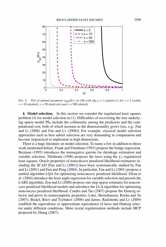
EXAMPLE 1. Assume that XM0 is orthonormal with M0 = {1, . . . , s} and|β0,1| = · · · = |β0,s |. Thus by (2),

y =s∑

j=1

β0,j xj = |β0,1|s∑

j=1

sgn(β0,j )xj .(28)

Let H be the linear subspace of Rn spanned by x1, . . . ,xs and H⊥ its orthog-onal complement. Further assume that p ≥ s + 1, xj ∈ H⊥ for each j ≥ s + 2,‖xs+1‖2 = 1, and

xs+1 = rs−1/2s∑

j=1

sgn(β0,j )xj + h with r ∈ (−1,1) and h ∈ H⊥.(29)

Then for any ε ∈ (0, |β0,1|), we have

maxj∈Mc

0

maxu∈Uε

|〈xj ,u〉| = maxu∈Uε

|〈xs+1,u〉| = maxv∈Vε

|〈xs+1,XM0 ρa(v)〉|

= |r|√sa(a + 1)/(a + |β0,1| − ε)2.

Thus condition (26) reduces to |r|√s a(a+1)

(a+|β0,1|−ε)2 ≤ 1 + a−1, which shows that for

any |r| > s−1/2, we have

aopt(ε) = |β0,1| − ε

(r2s)1/4 − 1.(30)

We see that the optimal parameter aopt(ε) is related to |β0,1| − ε through both r

and s. It approaches ∞ as |r| → s−1/2+ and goes to (|β0,1| − ε)/(s1/4 − 1) as|r| → 1− (see Figure 2). When |r| ≤ s−1/2, we have aopt(ε) = ∞ regardless ofε ∈ (0, |β0,1|).

In light of (28) and (29), r ∈ (−1,1) defining the noise predictor xs+1 is exactlythe correlation between xs+1 and y. Therefore in the noiseless setting (2), whenthe number of true variables s is large, the correlation r between the noise variablexs+1 and the response y has to be small in magnitude in order that the L1 penaltyis the optimal penalty, that is, aopt(ε) = ∞. Note that the cut-off point for |r| byour theory is s−1/2, while s−1/2 is exactly the absolute correlation between eachtrue variable xj and response y.

If we assume |β0,1| = minj∈M0 |β0,j | instead of |β0,j | = · · · = |β0,s |, then theright-hand side of (30) gives a lower bound on aopt(ε), which entails that the cut-off point for |r| by our theory can be above s−1/2. This result is sensible once weobserve that

| corr(xs+1,y)| ≤ |r| and max1≤j≤s

| corr(xj ,y)| = maxj∈M0 |β0,j |√∑sj=1(β0,j )2

≥ s−1/2,

where y = ∑si=1 β0,j xj . It is interesting to observe that the right-hand side of (30)

is positively related to minj∈M0 |β0,j |, which measures the strength of the weakestadditive component in the response.


FIG. 2. Plot of optimal parameter aopt(0+) in (30) with |β0,1| = 1 against |r| for s = 2 (solid),s = 10 (dashed), s = 50 (dash-dot) and s = 500 (dotted).

4. Model selection. In this section we consider the regularized least squaresproblem (4) for model selection in (1). Difficulties of recovering the true underly-ing sparse model M0 include the collinearity among the predictors and the com-putational cost, both of which increase as the dimensionality grows [see, e.g., Fanand Li (2006) and Fan and Lv (2008)]. For example, classical model selectionapproaches such as best subset selection are very demanding in computation andbecome impractical to implement in high dimensions.

There is a huge literature on model selection. To name a few in addition to thosework mentioned before, Frank and Friedman (1993) propose the bridge regression.Breiman (1995) introduces the nonnegative garrote for shrinkage estimation andvariable selection. Tibshirani (1996) proposes the lasso using the L1-regularizedleast squares. Oracle properties of nonconcave penalized likelihood estimators in-cluding the SCAD [Fan and Li (2001)] have been systematically studied by Fanand Li (2001) and Fan and Peng (2004). In particular, Fan and Li (2001) propose aunified algorithm LQA for optimizing nonconcave penalized likelihood. Efron etal. (2004) introduce the least angle regression for variable selection and present theLARS algorithm. Zou and Li (2008) propose one-step sparse estimates for noncon-cave penalized likelihood models and introduce the LLA algorithm for optimizingnonconcave penalized likelihood. Candes and Tao (2007) propose the Dantzig se-lector and prove its nonasymptotic properties. Later, Meinshausen, Rocha and Yu(2007), Bickel, Ritov and Tsybakov (2008) and James, Radchenki and Lv (2009)establish the equivalence or approximate equivalence of lasso and Dantzig selec-tor under different conditions. More recent regularization methods include MCPproposed by Zhang (2007).


Fan and Li (2001) point out the bias issue of lasso. Zou (2006) proposes theadaptive lasso to address this issue by using an adaptively weighted L1 penalty.Greenshtein and Ritov (2004) study the persistency of lasso-type procedures inhigh-dimensional linear predictor selection. Hunter and Li (2005) propose andstudy MM algorithms for variable selection. Li and Liang (2008) study variableselection for semiparametric regression models. Wang, Li and Tsai (2007) studythe problem of tuning parameter selection for the SCAD. Fan and Fan (2008) studythe impact of high dimensionality on classifications and propose the FAIR. Fan andLv (2008) propose the SIS as well as its extensions for variable screening and studyits asymptotic properties in ultra-high-dimensional feature space.

4.1. Regularized least squares estimator. We consider the regularized leastsquares problem (4) with the penalty pλ in the class satisfying Condition 1. Fora given regularization parameter λn ∈ [0,∞) indexed by sample size n, a p-di-mensional vector β

λn is conventionally called a regularized least squares estimatorof β0 if it is a (local) minimizer of (4). When the L2 penalty ρ(t) = t2 is used, theresulting estimator is called the ridge estimator, and its limit as λn → 0+ can be

easily shown to be the ordinary least squares estimator βols ≡ (XT X)+XT y, where

(·)+ denotes the Moore–Penrose generalized matrix inverse. βols

is also a solutionto the normal equation XT y = XT Xβ .

When λn ∈ (0,∞), Theorem 1 in Section 3.3 gives a sufficient condition on thestrict local minimizer of (4). From the proof of Theorem 1, we see that any localminimizer β

λn of (4) must satisfy

βλn

Mλn= Q−1XT

Mλny − �nλnQ−1ρ(β

λn

Mλn),(31)

‖zMcλn

‖∞ ≤ ρ′(0+),(32)

λmin(Q) ≥ �nλnκ(ρ; βλn

Mλn),(33)

where Mλn = supp(βλn

), Q = XTMλn

XMλn, z = (�nλn)

−1XT (y − Xβλn

), and

κ(ρ; βλn

Mλn) is given by (8). So there is generally a slight gap between the necessary

condition for local minimizer and sufficient condition for strict local minimizer, inview of (32), (33) and (19), (20). Hereafter the regularized least squares estimatoris referred to as a Z-estimator β

λn ∈ Rp that solves (31)–(33).We observe that β

λn

Mλnin (31) is the difference between two terms. The first term

Q−1XTMλn

y is exactly the ordinary least squares estimator by using predictors xj

with indices in Mλn . In the case of orthonormal design matrix X, we have Q = Isn

with sn = ‖βλn‖0, and thus the second term becomes �nλnρ(βλn

Mλn), which, for

nonzero components, has the same sign as βλn

Mλncomponentwise by definition. In


view of (31), we have

βλn

Mλn+ �nλnρ(β

λn

Mλn) = XT

Mλny,

which entails that both βλn

Mλnand �nλnρ(β

λn

Mλn) (for its nonzero components) have

the same sign as the ordinary least squares estimator XTMλn

y. This shows that the

second term above is indeed a shrinkage towards zero when X is orthonormal. Forthe penalties ρa introduced in Section 2.2, ρa(t) depends on both t and a [see (17)].In fact, for small a, ρa(t) takes a wide range of values when t varies, which ensuresthat ρa penalty shrinks the components of the ordinary least squares estimatordifferently. This gives us flexibility in model selection. It provides us a familyof regularized least squares estimators indexed by parameter a and regularizationparameter λn. As a becomes smaller, it generally gives sparser estimates.

4.2. Nonasymptotic properties. In this paper, we study a nonasymptotic prop-erty of β

λn , called the weak oracle property for simplicity, which means: (1) spar-sity in the sense of β

λn

Mc0= 0 with probability tending to 1 as n → ∞, and (2) con-

sistency under the L∞ loss. This property is weaker than the oracle property in-troduced by Fan and Li (2001). As mentioned before, we condition on the n × p

design matrix X.We use the pλ penalty in the class satisfying Condition 1 and make the following

assumptions on the deterministic design matrix X and the distribution of the noisevector ε in the linear model (1).

CONDITION 2. X satisfies

‖(XTM0

XM0)−1‖∞ ≤ C1n,(34)

‖XTMc

0XM0(X

TM0

XM0)−1‖∞ ≤ C2n,(35)

where M0 = supp(β0), C1n ∈ (0,∞), C2n ∈ [0,Cρ′(0+)ρ′(c0b0)

] for some C,c0 ∈ (0,1),b0 = minj∈M0 |β0,j |, and ‖ · ‖∞ denotes the matrix ∞-norm.

Here and below, ρ is associated with regularization parameter λn defined in (38)unless specified otherwise.

CONDITION 3. ε ∼ N(0, σ 2In) for some σ > 0.

When XM0 is orthonormal, the left-hand side of (35) becomes ‖XTMc

0XM0‖∞,

the maximum absolute sum of covariances between a noise variable and all s truevariables. Condition (35) constrains its growth rate. By the concavity of ρ in Con-dition 1, ρ ′(t) is decreasing in t ∈ [0,∞) and thus the ratio ρ ′(0+)/ρ′(c0b0) is


always no less than one. When the L1 penalty is used, C2n ∈ [0,C] and Condi-tion 2 reduces to the condition in Zhao and Yu (2006) and Wainwright (2006).

Condition 2 is an assumption on design matrix X. If we work with random de-sign, we can calculate the probability that Condition 2 holds by using the resultsfrom, for example, the random matrix theory. The Gaussian assumption in Condi-tion 3 can be relaxed to other light-tailed distributions so that we can derive similarexponential probability bounds.

CONDITION 4. There exists some γ ∈ (0, 12 ] such that[

D1n + ρ′(c0b0)

ρ′(0+)D2n

]C1n = O(n−γ ),(36)

where D1n = maxj∈M0 ‖xj‖2, D2n = maxj∈Mc0‖xj‖2 and X = (x1, . . . ,xp). Let

un ∈ (0,∞) satisfy limn→∞ un = ∞, λn ≤ λn, and

un ≤ [κ0(C2nD1n + D2n)]−1λmin(XTM0

XM0)(1 − C)ρ′(0+)σ−1,(37)

where

λn = �−1n

(C2nD1n + D2n)unσ

ρ′(0+) − C2nρ′(c0b0)and λn = C−1

1n (1 − c0)b0 − unD1nσ

�nρ′(c0b0;λn),(38)

C,c0 ∈ (0,1) are given in Condition 2, and κ0 = max{κ(ρ;b) :‖b − β0,M0‖∞ ≤

(1 − c0)b0} with κ(ρ;b) given by (8).

As seen later, we need the condition λn ≤ λn to ensure the existence of a de-sired regularization parameter λn = λn. Condition (37), which always holds whenκ0 = 0, is needed to ensure condition (33).

THEOREM 4 (Weak oracle property). Assume that pλ in (4) satisfies Condi-tion 1, Conditions 2–4 hold and p = o(une

u2n/2). Then there exists a regularized

least squares estimator βλn with regularization parameter λn = λn defined in (38)

such that with probability at least 1 − 2√πpu−1

n e−u2n/2, β

λn satisfies:

(a) (Sparsity) βλn

Mc0= 0;

(b) (L∞ loss) ‖βλn

M0− β0,M0

‖∞ ≤ h = O(n−γ un),

where M0 = supp(β0) and h = [D1n + ρ′(c0b0)ρ′(0+)

D2n]C1nun(1 − C)−1σ . As a con-

sequence, ‖βλn − β0‖2 = OP (√

sn−γ un), where s = ‖β0‖0.

We make some remarks on Theorem 4. In view of limn→∞ un = ∞ in Condi-tion 4, the dimensionality p is allowed to grow up exponentially fast with un. If κ0in (37) is of a small order, un can be allowed to be o(nγ ) and thus logp = o(n2γ ).


The diverging sequence (un) also controls the rate of the exponential probabil-ity bound. From Theorem 4, we see that with asymptotic probability one the L∞estimation loss of β

λn is bounded above by h1 + h2, where

h1 = D1nC1nun(1 − C)−1σ and h2 = ρ′(c0b0)

ρ′(0+)D2nC1nun(1 − C)−1σ.(39)

The second term h2 is associated with the penalty function ρ. For the L1 penalty,the ratio ρ ′(c0b0)/ρ

′(0+) is equal to one, and for other concave penalties, as men-tioned before, this ratio can be (much) smaller than one. This is consistent with thefact shown by Fan and Li (2001) that concave penalties can reduce the biases ofestimates.

In the classical setting of D1n,D2n = O(√

n) and C1n = O(n−1), we haveγ = 1/2 since ρ′(c0b0)/ρ

′(0+) ≤ 1 by Condition 1 and thus the consistency rateof β

λn under the L2 norm becomes OP (√

sn−1/2un), which is slightly slower than

OP (√

sn−1/2). This is because it is derived by using the L∞ loss of βλn in Theo-

rem 4(b). The use of the L∞ norm is due to the technical difficulty of proving theexistence of a solution to the nonlinear equation (31). We conjecture that by con-sidering the L2 norm directly, one can obtain the consistency rate OP (

√sn−1/2).

4.3. Choice of ρa penalty. Theorem 4 gives one characterization of the roleof penalty functions in regularized least squares for model selection in (1). Letus now consider the penalties ρa introduced in Section 2.2. We fix the divergingsequence (un) in Theorem 4 and see how the parameter a ∈ (0,∞] influences theperformance of the ρa-regularized least squares method.

In view of (11), we have

ρ′a(0+)

ρ′a(c0b0)

= (a + c0b0)2

a2 , a ∈ (0,∞) andρ′∞(0+)

ρ′∞(c0b0)= 1.(40)

Clearly ρ′a(0+)/ρ′

a(c0b0) is decreasing in a ∈ (0,∞]. Thus (35) in Condition 2becomes less restrictive as a → 0+. In view of (39) by Theorem 4, the upperbound on the L∞ estimation loss of the ρa-regularized least squares estimator β

λn

decreases to h1 as a approaches 0. However, in view of (12), the maximum con-cavity of ρa increases to ∞ as a → 0+. This suggests that the computational dif-ficulty of solving the ρa-regularized least squares problem (4) may increase as a

approaches 0. In practical implementation, we can adaptively choose a using thedata, for example, the cross-validation method.

5. Implementation. In this section, we discuss algorithms for solving regu-larization problems with ρa penalty. Specifically, the ρa-regularization problem (3)for sparse recovery in (2), and the ρa-regularized least squares problem (4) formodel selection in (1).


5.1. SIRS algorithm for sparse recovery. For any β = (β1, . . . , βp)T ∈ Rp , letD(β) = diag{d1, . . . , dp} and

v(β) = DXT (XDXT )+y,(41)

where D = D(β) and dj = β2j /ρa(|βj |) = (a + 1)−1|βj |(a + |βj |), j = 1, . . . , p.

We propose the sequentially and iteratively reweighted squares (SIRS) algorithmfor solving (3) with ρa penalty. SIRS uses the method of iteratively reweightedsquares and iteratively solves the ρ-regularization problem (3) with the weightedL2 penalty ρ(β) = βT �β , where � = diag{d−1

1 , . . . , d−1p } with D = D(γ ) for

some γ , 0−1 = ∞ and 0 · ∞ = 0. It sequentially searches for a good initial valuethat leads to β0. Pick a level of sparsity S, the number of iterations L, the numberof sequential steps M ≤ S and a small constant ε ∈ (0,1).

SIRS ALGORITHM.

1. Set k = 0.2. Initialize β(0) = 1 and set � = 1.3. Set β(�) ← v(β(�−1)) with D = D(β(�−1)) and � ← � + 1.4. Repeat step 3 until convergence or � = L + 1. Denote by β the resulting p-

vector.5. If ‖β‖0 ≤ S, stop and return β . Otherwise, set k ← k + 1 and repeat steps 2–4

with β(0) = I (|β| ≥ γk) + εI (|β| < γk) and γk the kth largest component of|β|, until stop or k = M . Return β .

In practice, we can set a small tolerance level for convergence and apply a hardthresholding with a sufficiently small threshold to β to generate sparsity in step 4.The small constant ε ∈ (0,1) is introduced to leverage the scoring of variables withindices in M0 = supp(β0) by suppressing the noise variables. Through numericalimplementations, we have found that SIRS is robust to the choice of ε. SIRS algo-rithm stops once it finds a sufficiently sparse solution to (2). We use a grid searchmethod to select the optimal parameter a of penalty ρa that produces the sparsestsolution.

5.1.1. Justification. It is nontrivial to derive the convergence of SIRS algo-rithm analytically. In all our numerical implementations, we have found that italways converges. In this section, we give a partial justification of SIRS.

For each given β(�−1), step 3 of SIRS solves the ρ-regularization prob-lem (3) with the weighted L2 penalty ρ(β) = βT �β , where � is given byD = D(β(�−1)). This can be easily shown by Proposition 1 and the identityv(β) = D1/2(D1/2XT XD1/2)+D1/2XT y. It follows from the definitions of D and �that ρa(β

(�−1)) = (β(�−1))T �β(�−1) = ρ(β(�−1)). Thus the two penalties agree atβ = β(�−1). Quadratic approximations have been used in many iterative algorithmssuch as LQA in Fan and Li (2001).

The following proposition characterizes lim�→∞ β(�) when it exists.


PROPOSITION 2. (a) If lim�→∞ β(�) exists, then it is a fixed point of the func-tional F :A → A,

F (γ ) = arg minβ∈A

βT �(γ )β,(42)

where A = {β ∈ Rp : y = Xβ} and �(γ ) denotes � given by D = D(γ ).(b) β0 is always a fixed point of the functional F .(c) Assume that p > n, spark(X) = n + 1 and ‖β0‖0 < (n + 1)/2. Then for any

fixed point β of the functional F , we have β = β0 or ‖β‖0 > (n + 1)/2.

5.1.2. Computational complexity. We now discuss the computational com-plexity of the SIRS algorithm. We first consider the case of p ≥ n. Note thatDXT (XDXT )+y = limλ→0+ DXT (λIn +XDXT )−1y. Thus in step 3, we can avoidcalculating the generalized matrix inverse and only need to calculate the p-vectorDXT (λIn + XDXT )−1y for a fixed sufficiently small λ ∈ (0,∞). Since the p × p

matrix D is diagonal, the computational complexity of λIn + XDXT is O(n2p). Itis known that inverting an n×n matrix is of computational complexity O(n3). Thisshows that the computational complexity of (λIn + XDXT )−1 is O(n2p) sincep ≥ n. Then it is easy to see that step 3 has computational complexity O(n2p).Similarly, when p ≤ n we can derive that step 3 has computational complex-ity O(np2) by using the identity v(β) = D1/2(D1/2XT XD1/2)+D1/2XT y, whichequals limλ→0+ D1/2(λIp + D1/2XT XD1/2)−1D1/2XT y. Therefore, the computa-tional complexity of the main step, step 3, of the SIRS algorithm is O(np(n∧p)),which is the same as that of the LARS algorithm [Efron et al. (2004)] for model se-lection. For given number of iterations L and number of sequential steps M , SIRShas computational complexity O(np(n ∧ p)LM). We would like to point out thatSIRS stops at any sequential step once it finds a sufficiently sparse solution to (2).

5.2. Model selection. Efficient algorithms for solving the regularized leastsquares problem (4) include the LQA proposed by Fan and Li (2001) and LLA in-troduced by Zou and Li (2008). In this paper we use LLA to solve (4) with ρa

penalty. For a fixed regularization parameter λn, LLA iteratively solves (4)by using local linear approximations of

∑pj=1 ρa(|βj |). At a given β(0) =

(β(0)1 , . . . , β

(0)p )T , LLA approximates

∑pj=1 ρa(|βj |) as

p∑j=1

[ρa

(∣∣β(0)j

∣∣) + ρ′a

(∣∣β(0)j

∣∣)(|βj | −∣∣β(0)

j

∣∣)].Then LLA solves the weighted lasso (L1-regularized least squares)

minβ∈Rp

{2−1‖y − Xβ‖2

2 + �nλn

p∑j=1

wj |βj |},(43)

where wj = ρ′a(|β(0)

j |) = a(a + 1)/(a + |β(0)j |)2, j = 1, . . . , p. We use a grid

search method to tune the parameter a of penalty ρa .


6. Numerical examples.

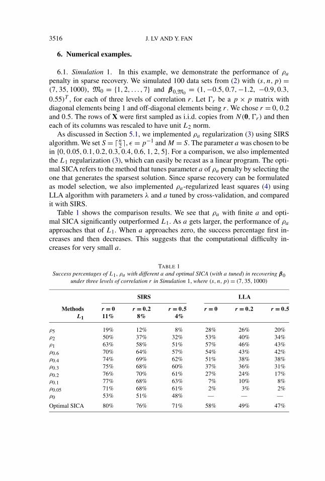
6.1. Simulation 1. In this example, we demonstrate the performance of ρa

penalty in sparse recovery. We simulated 100 data sets from (2) with (s, n,p) =(7,35,1000), M0 = {1,2, . . . ,7} and β0,M0

= (1,−0.5,0.7,−1.2, −0.9,0.3,

0.55)T , for each of three levels of correlation r . Let �r be a p × p matrix withdiagonal elements being 1 and off-diagonal elements being r . We chose r = 0, 0.2and 0.5. The rows of X were first sampled as i.i.d. copies from N(0,�r) and theneach of its columns was rescaled to have unit L2 norm.

As discussed in Section 5.1, we implemented ρa regularization (3) using SIRSalgorithm. We set S = �n

2�, ε = p−1 and M = S. The parameter a was chosen to bein {0,0.05,0.1,0.2,0.3,0.4,0.6,1,2,5}. For a comparison, we also implementedthe L1 regularization (3), which can easily be recast as a linear program. The opti-mal SICA refers to the method that tunes parameter a of ρa penalty by selecting theone that generates the sparsest solution. Since sparse recovery can be formulatedas model selection, we also implemented ρa-regularized least squares (4) usingLLA algorithm with parameters λ and a tuned by cross-validation, and comparedit with SIRS.

Table 1 shows the comparison results. We see that ρa with finite a and opti-mal SICA significantly outperformed L1. As a gets larger, the performance of ρa

approaches that of L1. When a approaches zero, the success percentage first in-creases and then decreases. This suggests that the computational difficulty in-creases for very small a.

TABLE 1Success percentages of L1, ρa with different a and optimal SICA (with a tuned) in recovering β0

under three levels of correlation r in Simulation 1, where (s, n,p) = (7,35,1000)

SIRS LLA

Methods r = 0 r = 0.2 r = 0.5 r = 0 r = 0.2 r = 0.5L1 11% 8% 4%

ρ5 19% 12% 8% 28% 26% 20%ρ2 50% 37% 32% 53% 40% 34%ρ1 63% 58% 51% 57% 46% 43%ρ0.6 70% 64% 57% 54% 43% 42%ρ0.4 74% 69% 62% 51% 38% 38%ρ0.3 75% 68% 60% 37% 36% 31%ρ0.2 76% 70% 61% 27% 24% 17%ρ0.1 77% 68% 63% 7% 10% 8%ρ0.05 71% 68% 61% 2% 3% 2%ρ0 53% 51% 48% — — —

Optimal SICA 80% 76% 71% 58% 49% 47%


6.2. Simulation 2. In this example as well as the next two ones, we demon-strate the performance of ρa penalty in model selection. The data were generatedfrom model (1). We set (n,p) = (100,50) and chose the true regression coeffi-cients vector β0 by setting M0 = {1,2, . . . ,7} and β0,M0

= (1,−0.5,0.7,−1.2,

−0.9,0.3,0.55)T . The number of simulations was 100. For each simulated dataset, the rows of X were sampled as i.i.d. copies from N(0,�0) with �0 =(0.5|i−j |)i,j=1,...,p , and ε was generated independently from N(0, σ 2In). Twonoise levels σ = 0.3 and 0.5 were considered. We compared SICA with lasso,SCAD and MCP. Lasso was implement by LARS algorithm, and SCAD, MCPand SICA were implemented by LLA algorithm. The regularization parameters λ

and a were selected by using a grid search method based on BIC, following Wang,Li and Tsai (2007).

Three performance measures were employed to compare the four methods. Thefirst measure is the prediction error (PE) defined as E(y − xT β)2, where β is theestimated coefficients vector by a method and x is an independent test point. Thesecond measure, #S, is the number of selected variables in the final model by amethod in a simulation. The third one, FN, measures the number of missed truevariables by a method in a simulation.

In the calculation of PE, an independent test sample of size 10,000 was gener-ated. All four methods had median FN = 0. Table 2 and Figure 3 summarize thecomparison results given by PE and #S.

6.3. Simulation 3. The setting of this example is the same as that of Simula-tion 2, except that (n,p) = (100,600) and σ = 0.1,0.3. Since p is larger than n,BIC breaks down in the tuning of λ and a. Thus we used five-fold cross-validationbased on prediction error to select the tuning parameters. All four methods hadmedian FN = 0. Table 3 and Figure 4 summarize the comparison results given byPE and #S. The boxplots of lasso are truncated to make it easier to view.

6.4. Real data analysis. In this example, we apply SICA to the diabetesdataset, which was studied by Efron et al. (2004). This dataset contains 10 base-line variables: age (age), sex (sex), body mass index (bmi), average blood pres-sure (bp) and 6 blood serum measurements (tc, ldl, hdl, tch, ltg, glu) for

TABLE 2Medians of PE and #S over 100 simulations for all methods in Simulation 2, where p = 50 and the

rows of X are i.i.d. copies from N(0,�0)

Measures Lasso SCAD MCP SICA

σ = 0.3 PE (×10−2) 12.88 9.77 9.38 9.97#S 13 7 7 7

σ = 0.5 PE (×10−1) 3.70 2.87 2.84 2.80#S 13 7 7 7


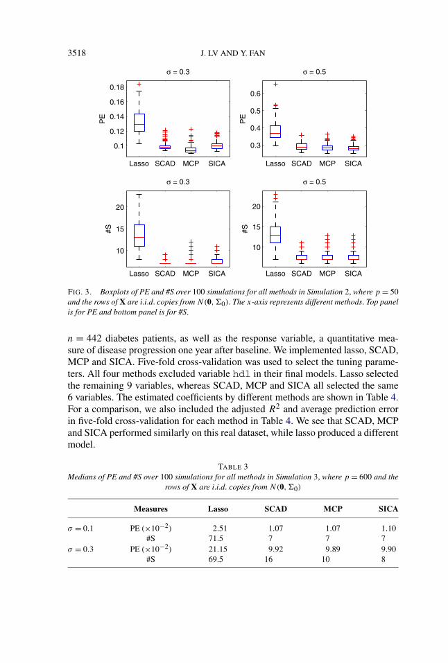
FIG. 3. Boxplots of PE and #S over 100 simulations for all methods in Simulation 2, where p = 50and the rows of X are i.i.d. copies from N(0,�0). The x-axis represents different methods. Top panelis for PE and bottom panel is for #S.

n = 442 diabetes patients, as well as the response variable, a quantitative mea-sure of disease progression one year after baseline. We implemented lasso, SCAD,MCP and SICA. Five-fold cross-validation was used to select the tuning parame-ters. All four methods excluded variable hdl in their final models. Lasso selectedthe remaining 9 variables, whereas SCAD, MCP and SICA all selected the same6 variables. The estimated coefficients by different methods are shown in Table 4.For a comparison, we also included the adjusted R2 and average prediction errorin five-fold cross-validation for each method in Table 4. We see that SCAD, MCPand SICA performed similarly on this real dataset, while lasso produced a differentmodel.

TABLE 3Medians of PE and #S over 100 simulations for all methods in Simulation 3, where p = 600 and the

rows of X are i.i.d. copies from N(0,�0)

Measures Lasso SCAD MCP SICA

σ = 0.1 PE (×10−2) 2.51 1.07 1.07 1.10#S 71.5 7 7 7

σ = 0.3 PE (×10−2) 21.15 9.92 9.89 9.90#S 69.5 16 10 8


FIG. 4. Boxplots of PE and #S over 100 simulations for all methods in Simulation 3, where p = 600and the rows of X are i.i.d. copies from N(0,�0). The x-axis represents different methods. Top panelis for PE and bottom panel is for #S.

7. Proofs.

7.1. Proof of Proposition 1. Let X = UDV be a singular value decompositionof X, where U and V are, respectively, n × n and p × p orthogonal matrices, D isan n×p matrix with its first k diagonal elements being d1, . . . , dk �= 0 and all other

TABLE 4Model coefficients obtained by all methods on the diabetes dataset, and their adjusted R2 [R2(adj)]

and average prediction errors (APE) based on five-fold cross-validation

Methods age sex bmi bp tc ldl

Lasso −6.4 −235.9 521.8 321.0 −568.6 301.6SCAD 0 −226.2 529.9 327.1 −757.6 538.3MCP 0 −226.3 529.9 327.2 −757.7 538.4SICA 0 −219.5 531.7 323.3 −743.1 525.0

hdl tch ltg glu R2(adj) APE

Lasso 0 143.9 669.6 66.8 50.73% 2956.9SCAD 0 0 804.1 0 50.82% 2939.5MCP 0 0 804.1 0 50.82% 2939.1SICA 0 0 800.2 0 50.82% 2935.8


elements being zero, and k = rank(X) ≤ n ∧ p. Then we have

β ∈ A ⇐⇒ y = Xβ ⇐⇒ UT y = UT Xβ = DVβ = Dβ(44)

⇐⇒ βi = d−1i wi, i = 1, . . . , k,

where β = (β1, . . . , βp)T = Vβ and UT y = (w1, . . . ,wn)T . Since V is orthogonal,

‖β‖2 = ‖β‖2 always holds. Thus it follows from (44) that

β2 = arg minβ∈A

‖β‖2 = VT β0,

where β0 = (d−11 w1, . . . , d

−1k wk,0, . . . ,0)T . It remains to show VT β0 = (XT ×

X)+XT y. By the above singular value decomposition of X, we have (XT X)+ =VT diag(a)V, where a = (d−2

1 , . . . , d−2k ,0, . . . ,0)T . Therefore, it is immediate to

see that

diag(a)DT UT y = (d−11 w1, . . . , d

−1k wk,0, . . . ,0)T = β0

and thus

(XT X)+XT y = VT diag(a)VVT DT UT y = VT β0.

This completes the proof.

7.2. Proof of Theorem 1. Fix an arbitrary βλ = (βλ

1 , . . . , βλp)T ∈ Rp and let

Mλ = supp(βλ). It follows from the classical optimization theory by taking differ-

entiation that if βλ

is a local minimizer of the regularized least squares problem (4)with λn = λ, there exists some v = (v1, . . . , vp)T ∈ Rp such that

XT Xβλ − XT y + �nλv = 0,(45)

where for j ∈ Mλ, vj = ρ(βλj ) and for j ∈ Mc

λ, vj ∈ [−ρ′(0+), ρ′(0+)]. More-

over, since βλ

is also a local minimizer of (4) constrained on the ‖βλ‖0-dimensional subspace {β ∈ Rp :βMc

λ= 0} of Rp , it is easy to show that

λmin(Q) ≥ �nλκ(ρ; βλ

Mλ),(46)

where Q = XTMλ

XMλand κ(ρ; βλ

Mλ) is given by (8). We will see below that

slightly strengthening the necessary condition (45) and (46) provides a sufficientcondition on the strict local minimizer of (4).

Since Q = XTMλ

XMλis nonsingular, β

λ

Mcλ= 0, vMλ

= ρ(βλ

Mλ) and ‖vMc

λ‖∞ ≤

ρ′(0+), (45) can, equivalently, be rewritten as

βλ

Mλ= Q−1XT

Mλy − �nλQ−1ρ(β

λ

Mλ),(47)

‖zMcλ‖∞ ≤ ρ ′(0+),(48)


where z = (�nλ)−1XT (y − Xβλ). Now we strengthen inequality (48) to strict in-

equality (19) and make an additional assumption (20). We will show that (18), (19)and (20) imply that β

λis a strict local minimizer of (4).

We first constrain the regularized least squares problem (4) on the ‖βλ‖0-dimensional subspace B = {β ∈ Rp :βMc

λ= 0} of Rp . It follows easily from con-

dition (20), the continuity of ρ′(t) in Condition 1, and the definition of κ(ρ; βλ

Mλ)

in (8) that the objective function in (4), �(β) ≡ 2−1‖y−Xβ‖22 +�n

∑pj=1 pλ(|βj |),

is strictly convex in a ball N0 in the subspace B centered at βλ. This along with

(18) immediately entails that βλ, as a critical point of �(·) in B, is the unique min-

imizer of �(·) in the neighborhood N0. Thus we have shown that βλ

is a strict localminimizer of �(·) in the subspace B.

It remains to prove that the sparse vector βλ

is indeed a strict local minimizerof �(·) on the whole space Rp . To show this, we will use condition (19). Take asufficiently small ball N1 in Rp centered at β

λsuch that N1 ∩ B ⊂ N0. Fix an

arbitrary γ 1 ∈ N1 \N0, we will show that �(γ 1) > �(βλ). Let γ 2 be the projection

of γ 1 onto the subspace B. Then it follows from N1 ∩B ⊂ N0 and the definitions

of B, N0 and N1 that γ 2 ∈ N0 ∩ N1, which entails that �(γ 2) > �(βλ) if γ 2 �=

βλ

by the strict convexity of �(·) in the neighborhood N0. We see that to prove�(γ 1) > �(β

λ), it suffices to show that �(γ 1) > �(γ 2).

It follows from the concavity of ρ in Condition 1 that ρ′(t) is decreasing in t ∈[0,∞). By condition (19) and the continuity of ρ′(t) in Condition 1, appropriatelyshrinking the radius of the ball N1 gives that there exists some δ ∈ (0,∞) suchthat ρ′(δ) ∈ (0, ρ′(0+)] and for any β ∈ N1,

‖wMcλ‖∞ < ρ′(δ),(49)

where w = (�nλ)−1XT (y − Xβ). We further shrink the radius of the ball N1 toless than δ. By the mean-value theorem, we have

�(γ 1) = �(γ 2) + ∇T �(γ 0)(γ 1 − γ 2),(50)

where γ 0 lies on the line segment joining γ 2 and γ 1 and γ 0 �= γ 2. Since

γ 1,γ 2 ∈ N1 and N1 is a ball centered at βλ

with radius less than δ, we have γ 0 =(γ0,1, . . . , γ0,p)T ∈ N1 and |γ0,j | < δ for any j ∈ Mc

λ. Note that by γ 1 ∈ N1 \ N0,we have

(γ 1 − γ2)Mλ= 0 and (γ 1 − γ 2)Mc

λ�= 0.

Let S = supp(γ 1) \ Mλ �= ∅ and γ 1 = (γ1,1, . . . , γ1,p)T . It is easy to seethat sgn(γ0,j ) = sgn(γ1,j ) for any j ∈ Mc

λ. Since γ 0 ∈ N1, by (49), (50) and


‖γ 0,Mcλ‖∞ < δ, we have

�(γ 1) − �(γ 2) = ∑j∈S

∂�(γ 0)

∂βj

γj = [XTS Xγ 0 − XT

S y + �nλρ(γ 0,S)]T γ 1,S

= −�nλ[(�nλ)−1XTS (y − Xγ 0)]T γ 1,S

+ �nλ∑j∈S

sgn(γ0,j )ρ′(|γ0,j |)γ1,j

> −�nλρ′(δ)‖γ 1,S‖1 + �nλ

∑j∈S

ρ′(|γ0,j |)|γ1,j |

≥ −�nλρ′(δ)‖γ 1,S‖1 + �nλ

∑j∈S

ρ′(δ)|γ1,j | = 0,

where we used the fact that ρ ′(|γ0,j |) ≥ ρ′(δ) since ρ′(t) is decreasing in t ∈[0,∞) and |γ0,j | < δ for any j ∈ S. This shows that �(γ 1) > �(γ 2), which con-cludes the proof.

7.3. Proof of Theorem 2. By (2), we have y = Xβ0. As mentioned before, tostudy the ρ-regularization problem (3), we consider the related ρ-regularized leastsquares problem (4) with y = Xβ0, �n = 1 and pλ(t) = λρ(t), t ∈ [0,∞). We will

construct a sequence of strict local minimizers βλ = (βλ

1 , . . . , βλp)T ∈ Rp of (4) for

a sequence of λ ∈ (0,∞) by using Theorem 1 and show that limλ→0+ βλ = β0.

Moreover, with some careful analysis we show that the limit β0 is indeed a localminimizer of (3).

Fix an arbitrary λ ∈ (0,∞) and βλ = (βλ

1 , . . . , βλp)T ∈ Rp . By Theorem 1, β

λ

will be a strict local minimizer of (4) as long as it satisfies conditions (18)–(20).We prove the existence of such a solution β

λwhen Mλ = supp(β

λ) = M0. Since

y = Xβ0 and κ(ρ; βλ

Mλ) ≤ κ(ρ) in view of (7) and (8), we can rewrite (18) and

(19) and strengthen (20) as

βλ

M0= β0,M0

− λQ−1ρ(βλ

M0),(51)

‖zMc0‖∞ < ρ′(0+),(52)

λmin(Q) > λκ(ρ),(53)

where z = XT XM0Q−1ρ(βλ

M0) and Q = XT

M0XM0 . Since Q is nonsingular and

κ(ρ) < ∞ by assumption, all λ ∈ (0, λ0) with λ0 = λmin(Q)/κ(ρ) automaticallysatisfy condition (53). We now consider λ ∈ (0, λ0). Assume that there exists someε ∈ (0,minj∈M0 |β0,j |) such that (22) holds. We will show that there exists a solu-

tion βλ

M0∈ Vε to (51) and (52), where Vε = ∏

j∈M0{t : |t − β0,j | ≤ ε}. Note that


condition (22) guarantees (52). So it remains to prove the existence of βλ

M0∈ Vε

to (51).Note that ρ′(t) is decreasing in t ∈ [0,∞) and thus ‖ρ(β

λ

M0)‖∞ ≤ ρ′(0+). Let

s = ‖β0‖0,

h = maxv∈Rs ,‖v‖∞≤ρ′(0+)

‖Q−1v‖∞

and λ1 = λ0 ∨ (ε/h). We now consider λ ∈ (0, λ1). Then for any γ ∈ Vε , we have

‖λQ−1ρ(γ )‖∞ ≤ λ1‖Q−1ρ(γ )‖∞ ≤ λ1h ≤ ε.

Thus by the continuity of the vector-valued function �(γ ) ≡ γ − β0,M0+

λQ−1ρ(γ ), an application of Miranda’s existence theorem [see, e.g., Vrahatis(1989)] shows that (51) indeed has a solution β

λ

M0in Vε .

For any λ ∈ (0, λ1), we have shown that (4) has a strict local minimizer βλ

suchthat supp(β

λ) = M0, β

λ

M0∈ Vε , and (51) holds. Note that by (51),

‖βλ − β0‖∞ = ‖βλ

M0− β0,M0

‖∞ = λ‖Q−1ρ(βλ

M0)‖∞ ≤ λh,

which entails that limλ→0+ βλ

exists and equals β0. It remains to prove that thelimit β0 is indeed a local minimizer of (3).

In view of the choice of λ and condition (22), it follows easily from (52), (53)and the proof of Theorem 1 that for each λ ∈ (0, λ1), β

λis the strict minimizer

of �(β) ≡ 2−1‖y − Xβ‖22 + λρ(β) on some common neighborhood C = {β ∈

Rp :βM0∈ Vε,‖βMc

0‖∞ ≤ δ} of βn,0, for some δ ∈ (0,∞) independent of λ. We

will show that β0 is the minimizer of (3) on the neighborhood N = C ∩ A of β0in the subspace A = {β ∈ Rp : y = Xβ}. Fix an arbitrary γ ∈ N . Since γ ∈ A andγ , β

λ ∈ C for each λ ∈ (0, λ1), it follows from (51), y = Xβ0 and Q = XTM0

XM0

that for each λ ∈ (0, λ1),

ρ(γ ) = λ−1�(γ ) ≥ λ−1�(βλ) = ρ(β

λ) + (2λ)−1‖y − Xβ

λ‖22

(54)= ρ(β

λ) + 2−1λρ(β

λ

M0)T Q−1ρ(β

λ

M0).

Note that by ‖ρ(βλ

M0)‖∞ ≤ ρ ′(0+), we have

0 ≤ ρ(βλ

M0)T Q−1ρ(β

λ

M0) ≤ λmin(Q)−1‖ρ(β

λ

M0)‖2

2

≤ λmin(Q)−1sρ′(0+)2.

Thus by limλ→0+ βλ = β0 and the continuity of ρ, letting λ → 0+ in (54) yields

ρ(γ ) ≥ ρ(β0). This completes the proof.


7.4. Proof of Theorem 3. By (25) and (12), the optimal penalty ρaopt(ε) satisfies

κ(ρaopt(ε)

) = infρa∈Pε

κ(ρa) = infρa∈Pε

2(a−1 + a−2)

(55)= sup{a ∈ (0,∞] :ρa ∈ Pε}.

Thus it follows from the definition of Pε in (24) that the optimal parameter aopt(ε)

is the largest a ∈ (0,∞] such that the following condition holds:

maxj∈Mc

0

maxu∈Uε

|〈xj ,u〉| ≤ ρ ′a(0+) = 1 + a−1,

where Uε = {XM0Q−1ρa(v) : v ∈ Vε} and Vε = ∏j∈M0

{t : |t − β0,j | ≤ ε}. It iseasy to see that for any ε ∈ (0,minj∈M0 |β0,j |), we have aopt(ε) > 0 since 1 +a−1 → ∞ and for each t �= 0, ρa(t) = t−2O(a) as a → 0+. This proves part (a).

Part (b) follows from two simple facts. First, it is clear that aopt(ε) = ∞ if andonly if

maxj∈Mc

0

maxu∈Uε

|〈xj ,u〉| ≤ 1,(56)

where Uε = {XM0Q−1 sgn(v) : v ∈ Vε} and Vε = ∏j∈M0

{t : |t − β0,j | < ε}.Second, for any ε ∈ (0,minj∈M0 |β0,j |), Uε contains a single point u0 =XM0Q−1 sgn(β0,M0

).

7.5. Proof of Theorem 4. We will prove that under the given regularity condi-tions, there exists a solution β

λn ∈ Rp to (31)–(33) with Mλn = supp(βλn

) = M0.Consider events

E1 = {‖XTM0

ε‖∞ ≤ unD1nσ } and E2 = {‖XTMc

0ε‖∞ ≤ unD2nσ },

where D1n and D2n are defined in Condition 4. Let ξ = (ξ1, . . . , ξp)T = XT ε. Itfollows from the definitions of D1n and D2n that

F1 = {|ξj | ≤ un‖xj‖2σ : j ∈ M0} ⊂ E1

and

F2 = {|ξj | ≤ un‖xj‖2σ : j ∈ Mc0} ⊂ E2,

where X = (x1, . . . ,xp). Since ε ∼ N(0, σ 2In) by Condition 3, we see that foreach j = 1, . . . , p, ξj has a N(0,‖xj‖2

2σ2) distribution. Thus an application of

the classical standard Gaussian tail probability bound and Bonferroni’s inequalitygives

P(E1 ∩ E2) ≥ P(F1 ∩ F2) ≥ 1 − [P(F c1 ) + P(F c

2 )]≥ 1 − [2sP (V > un) + 2(p − s)P (V > un)](57)

≥ 1 − 2√π

pu−1n e−u2

n/2,


where s = ‖β0‖0 and V is a standard Gaussian random variable. Hereafter wecondition on the event E1 ∩ E2. Under this event, we will show the existence ofa solution β

λn ∈ Rp to (31)–(33) with sgn(βλn

) = sgn(β0) and ‖βλn − β0‖∞ ≤(1 − c0)b0.

By Condition 4, we have λn ≤ λn, where

λn = �−1n

(C2nD1n + D2n)unσ

ρ′(0+) − C2nρ′(c0b0)and λn = C−1

1n (1 − c0)b0 − unD1nσ

�nρ′(c0b0;λn).(58)

Let λn be in the interval [λn,λn]. Since y = Xβ0 + ε by (1), (31) and (32) withMλn = M0 becomes

βλn

M0= β0,M0

− v,(59)

‖z‖∞ ≤ ρ ′(0+),(60)

where v = (XTM0

XM0)−1[�nλnρ(β

λn

M0) − XT

M0ε] and

z = XTMc

0XM0(X

TM0

XM0)−1ρ(β

λn

M0)

− (�nλn)−1[XT

Mc0XM0(X

TM0

XM0)−1XT

M0ε − XT

Mc0ε].

We first prove that (59) has a solution in N = {γ ∈ Rs :‖γ − β0,M0‖∞ ≤

(1 − c0)b0}. Fix an arbitrary γ ∈ N . By the concavity of ρ in Condition 1,ρ′(t) is decreasing in t ∈ [0,∞) and thus ‖ρ(γ )‖∞ ≤ ρ′(c0b0). This along with‖XT

M0ε‖∞ ≤ unD1nσ , (34) in Condition 2 and λn ≤ λn yields

‖(XTM0

XM0)−1[�nλnρ(γ ) − XT

M0ε]‖∞ ≤ (1 − c0)b0,

since ρ′(t;λ) is increasing in λ ∈ (0,∞) by Condition 1. Thus by the continuityof the vector-valued function �(γ ) ≡ γ − β0,M0

+ (XTM0

XM0)−1[�nλnρ(γ ) −

XTM0

ε], an application of Miranda’s existence theorem [see, e.g., Vrahatis (1989)]

shows that (59) indeed has a solution βλn

M0in N . It remains to check the inequality

(60) for βλn

M0∈ N . In fact it can be easily shown to hold by (35) in Condition 2

and ‖XTMc

0ε‖∞ ≤ unD2nσ , for λn = λn.

So far we have shown the existence of a solution βλn with λn = λn to (31) and

(32) with sgn(βλn

) = sgn(β0) and ‖βλn − β0‖∞ ≤ (1 − c0)b0 under the eventE1 ∩ E2. By (58), (59) and C2n ≤ C

ρ′(0+)ρ′(c0b0)

, letting λn = λn gives

‖βλn

M0− β0,M0

‖∞ = ‖(XTM0

XM0)−1[�nλnρ(β

λn

M0) − XT

M0ε]‖∞

≤ un

[D1n + ρ′(c0b0)

ρ′(0+)D2n

]C1n(1 − C)−1σ.


Note that condition (33) with λn = λn is guaranteed by (37) in Condition 4

since C2n ≤ Cρ′(0+)ρ′(c0b0)

. These along with sgn(βλn

) = sgn(β0), (36) in Condition 4

and (57) prove parts (a) and (b). Note that 1 − 2√πpu−1

n e−u2n/2 → 1 since p =

o(uneu2

n/2). Thus ‖βλn − β0‖2 = OP (√

sn−γ un) follows from parts (a) and (b)and

‖βλn

M0− β0,M0

‖2 ≤ √s‖βλn

M0− β0,M0

‖∞.

This concludes the proof.

7.6. Proof of Proposition 2. Part (a) follows directly from the definition ofβ(�) = v(β(�−1)). It is not hard to check that β0 is the unique minimizer of theweighted L2-regularization problem

minβ∈A

βT �(β0)β,

which entails immediately part (b). It remains to prove part (c). Clearly, it sufficesto show that for any β ∈ A, ‖β‖0 ≤ (n + 1)/2 implies β = β0. We prove this by acontradiction argument. Suppose there exists some β ∈ A with ‖β‖0 ≤ (n + 1)/2and β �= β0. Let γ = β − β0. Then we have γ �= 0 and Xγ = Xβ − Xβ0 = 0. But

‖γ ‖0 ≤ ‖β‖0 + ‖β0‖0 < (n + 1)/2 + (n + 1)/2 = n + 1 = spark(X),

which contradicts the definition of spark.

8. Discussion. We have studied the properties of regularization methods inmodel selection and sparse recovery under the unified framework of regularizedleast squares with concave penalties. We have provided regularity conditions underwhich the regularized least squares estimator enjoys a nonasymptotic weak oracleproperty for model selection, where the dimensionality can be of exponential or-der. Our results generalize those of Fan and Li (2001) and Fan and Peng (2004) inthe setting of regularized least squares. For sparse recovery, we have generalizeda sufficient condition identified for the L1 penalty to concave penalties, which en-sures the ρ/L0 equivalence. In particular, a family of penalties that give a smoothhomotopy between L0 and L1 penalties have been considered for both problems.Numerical studies further endorse our theoretical results and the advantage of ournew methods for model selection and sparse recovery.

It would be interesting to extend the results to regularization methods for thegeneralized linear models (GLMs) and more general models and loss functions.These problems are beyond the scope of this paper and will be interesting topicsfor future research.


Acknowledgments. We sincerely thank Professors Jianqing Fan and Jun S.Liu for constructive comments that led to improvement over an earlier version ofthis paper. We are deeply indebted to Professor Jianqing Fan for introducing us thetopic of high-dimensional variable selection and for his encouragement and helpfuldiscussions over the years. We gratefully acknowledge the helpful comments of theAssociate Editor and referees that substantially improved the presentation of thepaper.

REFERENCES

ANTONIADIS, A. and FAN, J. (2001). Regularization of wavelets approximations (with discussion).J. Amer. Statist. Assoc. 96 939–967. MR1946364

BICKEL, P. J. and LI, B. (2006). Regularization in statistics (with discussion). Test 15 271–344.MR2273731

BICKEL, P. J., RITOV, Y. and TSYBAKOV, A. (2008). Simultaneous analysis of Lasso and Dantzigselector. Ann. Statist. To appear.

BREIMAN, L. (1995). Better subset regression using the nonnegative garrote. Technometrics 37 373–384. MR1365720

CANDES, E. J. and TAO, T. (2005). Decoding by linear programming. IEEE Trans. Inform. Theory51 4203–4215. MR2243152

CANDES, E. J. and TAO, T. (2006). Near-optimal signal recovery from random projections: Univer-sal encoding strategies? IEEE Trans. Inform. Theory 52 5406–5425. MR2300700

CANDES, E. J. and TAO, T. (2007). The Dantzig selector: Statistical estimation when p is muchlarger than n (with discussion). Ann. Statist. 35 2313–2404. MR2382644

CANDÈS, E. J., WAKIN, M. B. and BOYD, S. P. (2008). Enhancing sparsity by reweighted �1minimization. J. Fourier Anal. Appl. 14 877–905.

CHEN, S., DONOHO, D. and SAUNDERS, M. (1999). Atomic decomposition by basis pursuit. SIAMJ. Sci. Comput. 20 33–61. MR1639094

DONOHO, D. L. (2004). Neighborly polytopes and sparse solution of underdetermined linear equa-tions. Technical report, Dept. Statistics, Stanford Univ.

DONOHO, D. L. and ELAD, M. (2003). Optimally sparse representation in general (nonorthogonal)dictionaries via �1 minimization. Proc. Natl. Acad. Sci. USA 100 2197–2202. MR1963681

DONOHO, D., ELAD, M. and TEMLYAKOV, V. (2006). Stable recovery of sparse overcomplete rep-resentations in the presence of noise. IEEE Trans. Inform. Theory 52 6–18. MR2237332

DONOHO, D. L. and JOHNSTONE, I. M. (1994). Ideal spatial adaptation by wavelet shrinkage.Biometrika 81 425–455. MR1311089

EFRON, B., HASTIE, T., JOHNSTONE, I. and TIBSHIRANI, R. (2004). Least angle regression (withdiscussion). Ann. Statist. 32 407–451. MR2060166

FAN, J. (1997). Comment on “Wavelets in statistics: A review” by A. Antoniadis. J. Italian Statist.Assoc. 6 131–138.

FAN, J. and FAN, Y. (2008). High-dimensional classification using features annealed independencerules. Ann. Statist. 36 2605–2637.

FAN, J. and LI, R. (2001). Variable selection via nonconcave penalized likelihood and its oracleproperties. J. Amer. Statist. Assoc. 96 1348–1360. MR1946581

FAN, J. and LI, R. (2006). Statistical challenges with high dimensionality: Feature selection inknowledge discovery. In Proceedings of the International Congress of Mathematicians (M. Sanz-Sole, J. Soria, J. L. Varona and J. Verdera, eds.) 3 595–622. European Math. Soc. PublishingHouse, Zürich. MR2275698

FAN, J. and LV, J. (2008). Sure independence screening for ultrahigh dimensional feature space(with discussion). J. Roy. Statist. Soc. Ser. B 70 849–911.

http://www.ams.org/mathscinet-getitem?mr=1946364














FAN, J. and PENG, H. (2004). Nonconcave penalized likelihood with diverging number of parame-ters. Ann. Statist. 32 928–961. MR2065194

FANG, K.-T. and ZHANG, Y.-T. (1990). Generalized Multivariate Analysis. Springer, Berlin.MR1079542

FRANK, I. E. and FRIEDMAN, J. H. (1993). A statistical view of some chemometrics regressiontools (with discussion). Technometrics 35 109–148.

FUCHS, J.-J. (2004). Recovery of exact sparse representations in the presence of noise. In Proceed-ings of IEEE International Conference on Acoustics, Speech, and Signal Processing 533–536.Montreal, QC.

GREENSHTEIN, E. and RITOV, Y. (2004). Persistence in high-dimensional linear predictor selectionand the virtue of overparametrization. Bernoulli 10 971–988. MR2108039

HUNTER, D. and LI, R. (2005). Variable selection using MM algorithms. Ann. Statist. 33 1617–1642. MR2166557

JAMES, G., RADCHENKO, P. and LV, J. (2009). DASSO: Connections between the Dantzig selectorand Lasso. J. Roy. Statist. Soc. Ser. B 71 127–142.

LI, R. and LIANG, H. (2008). Variable selection in semiparametric regression modeling. Ann. Statist.36 261–286. MR2387971

LIU, Y. and WU, Y. (2007). Variable selection via a combination of the L0 and L1 penalties. J. Com-put. Graph. Statist. 16 782–798.

MEINSHAUSEN, N., ROCHA, G. and YU, B. (2007). Discussion: A tale of three cousins: Lasso,L2Boosting and Dantzig. Ann. Statist. 35 2373–2384. MR2382649

NIKOLOVA, M. (2000). Local strong homogeneity of a regularized estimator. SIAM J. Appl. Math.61 633–658. MR1780806

TIBSHIRANI, R. (1996). Regression shrinkage and selection via the Lasso. J. Roy. Statist. Soc. Ser. B58 267–288. MR1379242

TROPP, J. A. (2006). Just relax: Convex programming methods for identifying sparse signals innoise. IEEE Trans. Inform. Theory 5 1030–1051. MR2238069

VRAHATIS, M. N. (1989). A short proof and a generalization of Miranda’s existence theorem. Proc.Amer. Math. Soc. 107 701–703. MR0993760

WAINWRIGHT, M. J. (2006). Sharp thresholds for high-dimensional and noisy recovery of sparsity.Technical report, Dept. Statistics, Univ. California, Berkeley.

WANG, H., LI, R. and TSAI, C.-L. (2007). Tuning parameter selectors for the smoothly clippedabsolute deviation method. Biometrika 94 553–568. MR2410008

ZHANG, C.-H. (2007). Penalized linear unbiased selection. Technical report, Dept. Statistics, Rut-gers Univ.

ZHAO, P. and YU, B. (2006). On model selection consistency of Lasso. J. Mach. Learn. Res. 72541–2563. MR2274449

ZOU, H. (2006). The adaptive Lasso and its oracle properties. J. Amer. Statist. Assoc. 101 1418–1429.MR2279469

ZOU, H. and LI, R. (2008). One-step sparse estimates in nonconcave penalized likelihood models(with discussion). Ann. Statist. 36 1509–1566. MR2435443

INFORMATION AND OPERATIONS

MANAGEMENT DEPARTMENT

MARSHALL SCHOOL OF BUSINESS

UNIVERSITY OF SOUTHERN CALIFORNIA

LOS ANGELES, CALIFORNIA 90089USAE-MAIL: [email protected]

[email protected]















mailto:[email protected]

mailto:[email protected]

a unified approach to model selection and sparse recovery ...jinchilv/publications/aos-lf09.pdf ·...

Documents