a unified treatment of evolving interfaces accounting for
TRANSCRIPT

A unified treatment of evolving interfaces accountingfor small deformations and atomic transport:grain-boundaries, phase transitions, epitaxy
Eliot Fried† and Morton E. Gurtin‡
†Department of Theoretical and Applied MechanicsUniversity of Illinois at Urbana-Champaign
Urbana, IL 61801-2935, USA
‡Department of Mathematical SciencesCarnegie Mellon University
Pittsburgh, PA 15213-3890, USA
Contents1 Introduction 4
1.1 Some important interface conditions . . . . . . . . . . . . . . . . . . . . . . . . . . . . . . 41.2 The need for a configurational force balance . . . . . . . . . . . . . . . . . . . . . . . . . . 61.3 A format for the study of evolving interfaces in the presence of deformation and atomic
transport . . . . . . . . . . . . . . . . . . . . . . . . . . . . . . . . . . . . . . . . . . . . . 71.4 The normal configurational force balance for a solid-vapor interface . . . . . . . . . . . . . 81.5 Scope . . . . . . . . . . . . . . . . . . . . . . . . . . . . . . . . . . . . . . . . . . . . . . . 9
A Deformation and atomic transport in bulk 102 Mechanics 10
3 Balance law for atoms 11
4 Thermodynamics. The free-energy imbalance 124.1 Chemical potentials. Balance of energy. Entropy imbalance . . . . . . . . . . . . . . . . . 124.2 Isothermal conditions. The free-energy imbalance . . . . . . . . . . . . . . . . . . . . . . . 13
5 Substitutional alloys 145.1 Lattice constraint. Vacancies . . . . . . . . . . . . . . . . . . . . . . . . . . . . . . . . . . 145.2 Substitutional flux constraint. Relative chemical potentials . . . . . . . . . . . . . . . . . 155.3 Elimination of the lattice constraint . . . . . . . . . . . . . . . . . . . . . . . . . . . . . . 17
6 Global theorems 18
7 Constitutive theory for multiple atomic species in the absence of a lattice constraint 207.1 Basic constitutive theory for an elastic material with Fickean diffusion . . . . . . . . . . . 207.2 Consequences of the thermodynamic restrictions . . . . . . . . . . . . . . . . . . . . . . . 227.3 Free enthalpy . . . . . . . . . . . . . . . . . . . . . . . . . . . . . . . . . . . . . . . . . . . 237.4 Mechanically simple materials . . . . . . . . . . . . . . . . . . . . . . . . . . . . . . . . . . 247.5 Cubic symmetry . . . . . . . . . . . . . . . . . . . . . . . . . . . . . . . . . . . . . . . . . 26
8 Digression: The Gibbs relation and Gibbs–Duhem equation at zero stress 27
1

2 E. Fried & M. E. Gurtin
9 Constitutive theory for a substitutional alloy 299.1 Larche–Cahn derivatives . . . . . . . . . . . . . . . . . . . . . . . . . . . . . . . . . . . . . 299.2 Constitutive equations . . . . . . . . . . . . . . . . . . . . . . . . . . . . . . . . . . . . . . 319.3 Thermodynamic restrictions . . . . . . . . . . . . . . . . . . . . . . . . . . . . . . . . . . . 339.4 Digression: positive definiteness of the mobility matrix . . . . . . . . . . . . . . . . . . . . 359.5 Free enthalpy. Moduli . . . . . . . . . . . . . . . . . . . . . . . . . . . . . . . . . . . . . . 369.6 Mechanically simple substitutional alloys . . . . . . . . . . . . . . . . . . . . . . . . . . . . 379.7 Cubic symmetry . . . . . . . . . . . . . . . . . . . . . . . . . . . . . . . . . . . . . . . . . 40
10 Governing equations 41
B Configurational forces in bulk 4211 Configurational forces. Power 43
11.1 Configurational force balance . . . . . . . . . . . . . . . . . . . . . . . . . . . . . . . . . . 4311.2 Migrating control volumes. Accretion . . . . . . . . . . . . . . . . . . . . . . . . . . . . . 4311.3 Power expended on a migrating control volume R(t) . . . . . . . . . . . . . . . . . . . . . 45
12 Thermodynamical laws for migrating control volumes. The Eshelby relation 4612.1 Migrational balance laws . . . . . . . . . . . . . . . . . . . . . . . . . . . . . . . . . . . . . 4612.2 The Eshelby relation as a consequence of invariance . . . . . . . . . . . . . . . . . . . . . 4712.3 Consistency of the migrational balance laws with classical forms of these laws . . . . . . . 4912.4 Isothermal conditions. The free-energy imbalance . . . . . . . . . . . . . . . . . . . . . . . 4912.5 Generic free-energy imbalance for migrating control volumes . . . . . . . . . . . . . . . . . 50
13 Role and influence of constitutive equations 50
C Interface kinematics 5214 Definitions and basic results 52
14.1 Curvature. Normal velocity. Normal time-derivative . . . . . . . . . . . . . . . . . . . . . 5214.2 Commutator and transport identities . . . . . . . . . . . . . . . . . . . . . . . . . . . . . . 5414.3 Evolving subcurves C(t) of S(t) . . . . . . . . . . . . . . . . . . . . . . . . . . . . . . . . . 5514.4 Transport theorem for integrals . . . . . . . . . . . . . . . . . . . . . . . . . . . . . . . . . 57
15 Deformation of the interface 5715.1 Interfacial limits . . . . . . . . . . . . . . . . . . . . . . . . . . . . . . . . . . . . . . . . . 5715.2 Interfacial-strain vector . . . . . . . . . . . . . . . . . . . . . . . . . . . . . . . . . . . . . 58
16 Interfacial pillboxes 59
D Grain boundaries 6017 Simple theory neglecting deformation and atomic transport 60
17.1 Configurational force balance . . . . . . . . . . . . . . . . . . . . . . . . . . . . . . . . . . 6117.2 Power . . . . . . . . . . . . . . . . . . . . . . . . . . . . . . . . . . . . . . . . . . . . . . . 6217.3 Free-energy imbalance . . . . . . . . . . . . . . . . . . . . . . . . . . . . . . . . . . . . . . 6317.4 Constitutive equations . . . . . . . . . . . . . . . . . . . . . . . . . . . . . . . . . . . . . . 6617.5 Evolution equation for the grain boundary. Parabolicity and backward parabolicity . . . . 6817.6 Backward parabolicity. Facets and wrinklings . . . . . . . . . . . . . . . . . . . . . . . . . 7017.7 Junctions . . . . . . . . . . . . . . . . . . . . . . . . . . . . . . . . . . . . . . . . . . . . . 7117.8 Digression: general theory of interfacial constitutive relations with essentially linear dis-
sipative response . . . . . . . . . . . . . . . . . . . . . . . . . . . . . . . . . . . . . . . . . 72
18 Interfacial couples. Allowance for an energetic dependence on curvature 7418.1 Configurational torque balance . . . . . . . . . . . . . . . . . . . . . . . . . . . . . . . . . 7418.2 Power . . . . . . . . . . . . . . . . . . . . . . . . . . . . . . . . . . . . . . . . . . . . . . . 7518.3 Free-energy imbalance . . . . . . . . . . . . . . . . . . . . . . . . . . . . . . . . . . . . . . 7718.4 Constitutive equations . . . . . . . . . . . . . . . . . . . . . . . . . . . . . . . . . . . . . . 7818.5 Evolution equation for the grain boundary . . . . . . . . . . . . . . . . . . . . . . . . . . . 78

A unified treatment of evolving interfaces 3
19 Grain-vapor interfaces with atomic transport 7919.1 Configurational force balance . . . . . . . . . . . . . . . . . . . . . . . . . . . . . . . . . . 7919.2 Power . . . . . . . . . . . . . . . . . . . . . . . . . . . . . . . . . . . . . . . . . . . . . . . 8019.3 Atomic flows due to diffusion, evaporation-condensation, and accretion. Atomic balance . 8019.4 Free-energy imbalance . . . . . . . . . . . . . . . . . . . . . . . . . . . . . . . . . . . . . . 8119.5 Constitutive equations . . . . . . . . . . . . . . . . . . . . . . . . . . . . . . . . . . . . . . 8319.6 Basic equations . . . . . . . . . . . . . . . . . . . . . . . . . . . . . . . . . . . . . . . . . . 8419.7 Nearly flat interface at equilibrium . . . . . . . . . . . . . . . . . . . . . . . . . . . . . . . 85
E Strained solid-vapor interfaces. Epitaxy 87
20 Configurational and standard forces 8720.1 Configurational forces . . . . . . . . . . . . . . . . . . . . . . . . . . . . . . . . . . . . . . 8820.2 Standard forces . . . . . . . . . . . . . . . . . . . . . . . . . . . . . . . . . . . . . . . . . . 88
21 Power 8921.1 External power expenditures . . . . . . . . . . . . . . . . . . . . . . . . . . . . . . . . . . 8921.2 Internal power expenditures. Power balance . . . . . . . . . . . . . . . . . . . . . . . . . . 90
22 Atomic transport 9122.1 Atomic balance . . . . . . . . . . . . . . . . . . . . . . . . . . . . . . . . . . . . . . . . . . 9122.2 Net atomic balance . . . . . . . . . . . . . . . . . . . . . . . . . . . . . . . . . . . . . . . . 92
23 Free-energy imbalance 9323.1 Energy flows due to atomic transport. Global imbalance . . . . . . . . . . . . . . . . . . . 9323.2 Dissipation inequality . . . . . . . . . . . . . . . . . . . . . . . . . . . . . . . . . . . . . . 94
24 Normal configurational force balance revisited 9624.1 Mechanical potential F . . . . . . . . . . . . . . . . . . . . . . . . . . . . . . . . . . . . . 9624.2 Substitutional alloys. Interfacial chemical potentials µα in terms of the relative chemical-
potentials µαβ . . . . . . . . . . . . . . . . . . . . . . . . . . . . . . . . . . . . . . . . . . 97
25 Constitutive equations for the interface 9825.1 General relations . . . . . . . . . . . . . . . . . . . . . . . . . . . . . . . . . . . . . . . . . 9825.2 Uncoupled relations for hα and g . . . . . . . . . . . . . . . . . . . . . . . . . . . . . . . . 100
26 Governing equations at the interface 10026.1 Equations with adatom densities included . . . . . . . . . . . . . . . . . . . . . . . . . . . 10026.2 Equations when adatom densities are neglected . . . . . . . . . . . . . . . . . . . . . . . . 10426.3 Addendum: Importance of the kinetic term g = −bV . . . . . . . . . . . . . . . . . . . . . 108
27 Interfacial couples. Allowance for an energetic dependence on curvature 109
28 Allowance for evaporation-condensation 113
F Coherent phase transitions 115
29 Forces. Power 11529.1 Configurational forces . . . . . . . . . . . . . . . . . . . . . . . . . . . . . . . . . . . . . . 11529.2 Standard forces . . . . . . . . . . . . . . . . . . . . . . . . . . . . . . . . . . . . . . . . . . 11529.3 Power . . . . . . . . . . . . . . . . . . . . . . . . . . . . . . . . . . . . . . . . . . . . . . . 116
30 Atomic transport 117
31 Free-energy imbalance 11831.1 Dissipation inequality for unconstrained materials . . . . . . . . . . . . . . . . . . . . . . . 11931.2 Interfacial flux constraint and free-energy imbalance for substitutional alloys . . . . . . . . 119
32 Global theorems 121

4 E. Fried & M. E. Gurtin
33 Normal configurational force balance revisited 12233.1 General relation . . . . . . . . . . . . . . . . . . . . . . . . . . . . . . . . . . . . . . . . . . 12233.2 Substitutional alloys . . . . . . . . . . . . . . . . . . . . . . . . . . . . . . . . . . . . . . . 12333.3 Alternative forms for G . . . . . . . . . . . . . . . . . . . . . . . . . . . . . . . . . . . . . . 123
34 Constitutive equations for the interface 124
35 General equations for the interface 125
Appendices 126A Justification of the free-energy conditions (9.45) at zero stress. Gibbs relation 126
B Equivalent formulations of the basic laws. Control-volume equivalency theorem 128
C Status of the theory as an approximation of the finite-deformation theory 131C.1 Theory for finite deformations . . . . . . . . . . . . . . . . . . . . . . . . . . . . . . . . . . 132C.2 Theory for small deformations as an approximation of the finite-deformation theory . . . 136
1 Introduction
This review presents a unified treatment of several topics at the intersection of contin-uum mechanics and materials science; the thrust concerns processes involving evolvinginterfaces, focusing on grain-boundaries, solid-vapor interfaces (with emphasis on epi-taxy), and coherent phase-transitions. Central to our discussion is the interaction ofdeformation, atomic transport, and accretion within a dissipative, dynamical framework,but as our interest is crystalline materials, we restrict our attention to small deforma-tions.1 To avoid geometrical complications associated with surfaces in R
3, we work intwo space-dimensions when discussing interfaces, but in R
3 when discussing the theoryin bulk.
1.1 Some important interface conditions
The past half-century has seen much activity among materials scientists and mechaniciansconcerning interface problems, a central outcome being the realization that such problemsgenerally result in an interface equation over and above those that follow from the classicalbalances for forces, moments, and mass. This extra interface condition takes a variety offorms, the most important examples being:
(i) Herring’s equation (1951). This is an equation,
U = −(
ψ +∂2ψ
∂ϑ2
)
K, (1.1)
relating the chemical potential U of a solid-vapor interface to its curvature K. Hereψ(ϑ) > 0 is the free-energy (density) of the interface with ϑ = ϑ(x) the orientation;that is, the counterclockwise angle to the interface tangent t (Figure 10, page 69).Invoking an assumption of local equilibrium, Herring defines the chemical potentialas the variational derivative of the total free energy with respect to variations inthe configuration of the interface. Following Herring, Wu (1996), Norris (1998),and Freund (1998), generalizing earlier work of Asaro and Tiller (1972) and Riceand Chuang (1981), compute the chemical potential of a solid-vapor interface in the
1Most applications in which deformation, atomic transport, and accretion are present involve smalldeformations. An abbreviated account of the formal analysis involved in the approximation of smalldeformations within a finite-deformational framework is provided in Appendix C.

A unified treatment of evolving interfaces 5
presence of deformation, allowing for interfacial stress. Their result, which allowsfor finite deformations, is, when set within a framework of small deformations,given by
U = Ψ− Tn · (∇u)n − γn · Tt − (ψ − σε)K − ∂τ
∂s. (1.2)
Here Ψ is the bulk free-energy (density); T is the bulk stress; u is the displacement;n and t are the interface normal and tangent; s denotes arc length;
ε = t · (∇u)t and γ = n · (∇u)t
are the tensile and shear strains within the interface. The result (1.2) is derivedvariationally; consequently, it is based on a constitutive equation
ψ = ψ(ε,ϑ)
for the interfacial free-energy, with σ and τ defined by
σ =∂ψ(ε,ϑ)∂ε
, τ =∂ψ(ε,ϑ)∂ϑ
.
The presence of the shear strain γ in (1.2) is a consequence of our assumptionof small deformations. Specifically, it follows from the fact that the interfacialstress s = σt is tangent to the interface, but the interfacial strain (∇u)t is not (cf.Footnote 68, page 91).
(ii) Mullins’s equations (1956, 1957). These are geometric equations,
bV = ψK and V = −(
Lψ
ρ2
)∂2K
∂s2, (1.3)
for the respective motions of an isotropic grain-boundary and an isotropic grain-vapor interface, neglecting evaporation-condensation. Here V is the (scalar) normalvelocity of the grain-boundary (or interface) S, while ψ, b, ρ, and L are strictlypositive constants, with ψ the interfacial free-energy (density), b a kinetic modulus(or, reciprocal mobility), ρ the atomic density of the solid, and L the mobility forFickean diffusion within S. Mullins’s argument in support of (1.3)1 is physicalin nature and based on work of Smoluchowski (1951), Turnbull (1951), and Beck(1952). To derive (1.3)2, Mullins appeals to balance of mass supplemented by Fick’slaw and Herring’s equation (1.1) for the chemical potential.
(iii) Kinetic Maxwell equation. This is a condition
[[
Ψ−N∑
α=1
ραµα − Tn · (∇u)n]]
= bV. (1.4)
for a propagating coherent phase interface between two phases composed of atomicspecies α = 1, 2, . . . , N . Here, µα and ρα are the chemical potentials and atomicdensities in bulk, [[f ]] represents the jump in a field f across the interface, and, asin (1.3)1, b is a constitutively determined kinetic modulus. The kinetic Maxwellcondition was first obtained by Heidug and Lehner (1985), Truskinovsky (1987),and Abeyaratne and Knowles (1990), who ignored atomic diffusion but allowed for
6 E. Fried & M. E. Gurtin
both inertia and finite deformations.2 Their derivations are based on determiningthe energy dissipation, per unit interfacial area, associated with the propagationof the interface and then appealing to the second law. When the kinetic modulusb = 0, (1.4) reduces to the classical Maxwell equation
[[
Ψ−N∑
α=1
ραµα − Tn · (∇u)n]]
= 0,
which was first derived variationally by Larche and Cahn (1978).3
(iv) Leo–Sekerka relation (1989). This is a condition for an interface in equilibrium.Relying on a variational framework set forth by Larche and Cahn (1978) (cf., also,Alexander and Johnson, 1985; Johnson and Alexander, 1986), Leo and Sekerka con-sider coherent and incoherent solid-solid interfaces as well as solid-fluid interfaces,and allow for finite deformations. For an interface between a vapor and an alloycomposed of atomic species α = 1, 2, . . . , N , neglecting vapor pressure and thermalinfluences and assuming small deformations, the Leo–Sekerka relation takes theform
N∑
α=1
(ρα − δαK)µα = Ψ− Tn · (∇u)n − γn · Tt − (ψ − σε)K − ∂τ
∂s. (1.5)
The relation (1.5) is based on a constitutive equation
ψ = ψ(ε,ϑ,+δ ), +δ = (δ1, δ2, . . . , δN ),
for the interfacial free-energy, supplemented by the definitions
σ =∂ψ(ε,ϑ,+δ )
∂ε, τ =
∂ψ(ε,ϑ,+δ )∂ϑ
, µα =∂ψ(ε,ϑ,+δ )
∂δα.
Here δα are the interfacial atomic-densities of species α.
1.2 The need for a configurational force balance
One cannot deny the applicability of the interface conditions (1.1)–(1.5); nor can one denythe great physical insight underlying their derivation. But in studying these derivationsone is left trying to ascertain the status of the resulting equations (1.1)–(1.5): are theybalances, or constitutive equations, or neither?4 This and the disparity between thephysical bases underlying their derivation would seem to at least indicate the absence ofa basic unifying principle.
That additional configurational forces5 may be needed to describe phenomena asso-ciated with the material itself is clear from the seminal work of Eshelby (1951, 1956,1970, 1975), Peach and Koehler (1950), and Herring (1951) on lattice defects. But these
2Under these circumstances, the kinetic Maxwell condition is (1.4) with µα = 0, α = 1, 2, . . . , N ,and with T the first Piola–Kirchhoff stress. Although the first derivations ignored atomic diffusion, itsinclusion is straightforward.
3Cf. also Eshelby (1970), Robin (1974), Grinfeld (1981), James (1981), and Gurtin (1983), who neglectcompositional effects.
4Successful theories of continuum mechanics are typically based on a clear separation of balancelaws and constitutive equations; the former describing large classes of materials, the latter describingparticular materials.
5We use the term configurational to differentiate these forces from classical Newtonian forces, whichwe refer to as standard.

A unified treatment of evolving interfaces 7
studies are based on variational arguments, arguments that, by their very nature, cannotcharacterize dissipation. Moreover, the introduction of configurational forces throughsuch formalisms is, in each case, based an underlying constitutive framework and hencerestricted to a particular class of materials.6
A completely different point of view is taken by Gurtin and Struthers (1990),7 who— using an argument based on invariance under observer changes — conclude that aconfigurational force balance should join the standard (Newtonian) force balance as abasic law of continuum physics. Here the operative word is “basic”. Basic laws areby their very nature independent of constitutive assumptions; when placed within athermodynamic framework such laws allow one to use the now standard procedures ofcontinuum thermodynamics to develop suitable constitutive theories.
1.3 A format for the study of evolving interfaces in the presenceof deformation and atomic transport
We here develop a complete theory of evolving interfaces in the presence of deformationand atomic transport using a format based on:
(a) Standard (Newtonian) balance laws for forces and moments that account for stan-dard stresses in bulk and within the interface.
(b) An independent balance law for configurational forces that accounts for configura-tional stresses in bulk and within the interface.8
(c) Atomic balances, one for each atomic species. These balances account for bulk andsurface diffusion.
(d) A mechanical (isothermal) version of the second law in the form of a free-energyimbalance. This imbalance, which accounts for temporal changes in free-energy,energy flows due to atomic transport, and power expended by both standard andconfigurational forces, may be derived as a consequence of more typical forms ofthe first two laws under isothermal conditions.
(e) Thermodynamically consistent constitutive relations for the interface and for theinteraction between the interface and its environment.
We show that each of the interface conditions in (i)–(iv) may be derived withinthis framework without assumptions of local equilibrium. One of the more interestingoutcomes of the format we use is an explicit relation for the configurational surfacetension σ in terms of other interfacial fields; viz.,
σ = ψ −N∑
α=1
δαµα − σε. (1.6)
This relation, a direct consequence of the free-energy imbalance applied to the interface,is a basic relation valid for all isothermal interfaces, independent of constitutive assump-tions and hence of material; it places in perspective the basic difference between the
6A vehicle for the discussion of configurational forces within a dynamical, dissipative frameworkderives configurational force balances by manipulating the standard momentum balance, supplementedby hypereslastic constitutive relations (e.g., Maugin, 1993). But such derived balances, while interesting,are satisfied automatically whenever the momentum balance is satisfied and are hence superfluous.
7This work is rather obtuse; better references for the underlying ideas are Gurtin (1995, 2000).8As extended by Davı and Gurtin (1990), Gurtin (1991), Gurtin and Voorhees (1995), and Fried and
Gurtin (1999, 2003) to account for atomic transport.

8 E. Fried & M. E. Gurtin
configurational surface tension σ and standard surface stress σ (cf. Footnote 72). Thereis much confusion in the literature concerning surface tension σ and its relation to surfacefree-energy ψ. By (1.6), we see that these two notions coincide if and only if standardinterfacial stress as well as interfacial atomic densities are negligible.
1.4 The normal configurational force balance for a solid-vaporinterface
To illustrate the format described above, we consider the special case of a solid-vaporinterface discussed in Part E. In this case, neglecting the vapor pressure (and henceconfigurational forces exerted by the vapor on the interface), the configurational forcebalance for the interface takes the simple form
∂c∂s
+ g = Cn.
Here c is the configurational surface stress, g is an internal force associated with the at-tachment kinetics of vapor atoms at the solid surface, and C is the limit, at the interface,of the configurational stress in the solid. The tangential and normal components of c,
σ = c · t, τ = c · n,
are the configurational surface tension and the configurational shear;9 the theory in bulkshows C to be the Eshelby tensor
C =(
Ψ−N∑
α=1
ραµα
)
1 − (∇u)!T (1.7)
(cf. (12.15)). Of most importance is the component
σK +∂τ
∂s+ g = n · Cn, g = g · n,
of the configurational force balance normal to the interface, as this is the componentrelevant to the motion of the interface.
For a solid-vapor interface in the presence of deformation and atomic transport, thenormal configurational force balance, when combined with (1.6), (1.7), and the standardforce, moment, and atomic balances, yields the interface condition (Fried and Gurtin,2003)
N∑
α=1
(ρα − δαK)µα = Ψ− Tn · (∇u)n − γn · Tt − (ψ − σε)K − ∂τ
∂s− g, (1.8)
with σ the standard surface-tension. This balance is basic, as its derivation utilizes onlybasic laws; as such it is independent of material. A consequence of the theory is that,thermodynamically, the force g is conjugate to the normal velocity V of the interface,and dissipative. Within a constitutive framework, thermodynamics renders this forceoften, but not always, of the form g = −bV , with b ≥ 0 a kinetic modulus. The forceg represents the sole dissipative force associated with the exchange of atoms betweenthe solid and the vapor at the interface, the corresponding energy dissipated, per unitinterfacial area, being −gV .
9Thus, in contrast to more classical discussions, the surface tension actually represents a force tangentto the interface, with no a priori relationship to surface energy.

A unified treatment of evolving interfaces 9
If we take g ≡ 0, then the normal configurational force balance (1.8) reduces to theLeo–Sekerka relation (1.5). The Leo–Sekerka relation follows rigorously as an Euler–Lagrange equation associated with the variational problem of minimizing the total freeenergy of a solid particle surrounded by a vapor. Thus, for solid-vapor interfaces inequilibrium, the format adopted here is completely consistent with results derived vari-ationally.
The Leo–Sekerka relation (or similar relations for other types of phase interfaces)is typically applied, as is, to dynamical problems, often with an accompanying appealto an hypothesis of “local equilibrium”, although the precise meaning of this assump-tion is never spelled out. Within the more general framework leading to the normalconfigurational force balance (1.8), the question as to when the Leo–Sekerka relation isapplicable is equivalent to the question as to when the internal force g is negligible. Ourmore general framework provides an answer to this question: for sufficiently small lengthscales the internal force g cannot be neglected, because the term emanating from g inthe evolution equations for the interface is of the same order of magnitude as the otherkinetic term in these equations, which results from accretion (cf. §26.3). On the otherhand, for sufficiently large length scales the force g is negligible. Quantification of theterms “small” and “large” would require a knowledge of the kinetic modulus b.
If we restrict attention to a single atomic species, neglect the adatom density, and takeg = 0, then the normal configurational force balance reduces to the Wu–Norris–Freundrelation (1.2) with U = ρµ. The chemical potential U of Wu, Norris, and Freund is, byits very definition, a potential associated with the addition of material at the solid-vaporinterface, without regard to the specific composition of that material. As such, U cannotbe used to discuss alloys.
1.5 Scope
We begin with a discussion of the theory in bulk, as this allows for a simple presentationof basic ideas. Our discussion of substitutional alloys follows Larche and Cahn (1985),10who introduce a scalar constant, ρsites, that represents the density of substitutional sites,per unit volume, available for occupation by atoms. The atomic densities ρα for asubstitutional alloy are then required to satisfy the lattice constraint
N∑
α=1
ρα = ρsites,
a constraint that Larche and Cahn show to have important consequences, the mostimportant being the result that Fickean diffusion in bulk is driven not by the individualchemical potentials µα, but instead by the relative chemical potentials µαβ = µα − µβ .Larche and Cahn arrive at this result using a variational argument. Here following theframework set forth in §1.3, we show that this result of Larche and Cahn is independentof constitutive equations, as it follows directly from the bulk free-energy imbalance andthe requirement that the bulk atomic-fluxes α satisify the substitutional flux constraint
N∑
α=1
α = 0
(Agren (1982), Cahn and Larche (1983)).To arrive at thermodynamically consistent equations, we follow Coleman and Noll
(1963), who use the laws of continuum thermodynamics to suitably restrict constitutive10Mechanicians seem unaware of this work.

10 E. Fried & M. E. Gurtin
equations. This process involves differentiating the constitutive relation for the bulkfree-energy with respect to atomic densities. For substitutional alloys any such differen-tiation must respect the lattice constraint. We overcome this obstacle with the aid ofthe Larche–Cahn derivative (Larche and Cahn, 1985), a procedure that results in consti-tutive relations for the relative chemical potentials. To our knowledge, ours is the firstwork to combine the approach of Coleman and Noll with that of Larche and Cahn.
We consider also unconstrained materials, which are materials whose atomic densitiesare unencumbered by a lattice constraint. A material whose mobile atoms are interstitialwould be unconstrained, as the high density of interstitial vacancies renders a latticeconstraint unimportant. More generally, some workers (cf. Mullins and Sekerka 1985)circumvent the discussion of a lattice constraint by assuming the existence of a defectmechanism that accomodates an excess or deficiency of substitutional atoms; materialstreated under such an assumption are, by fiat, unconstrained.
Our discussion of interfaces is based on the format presented in §1.3. We begin with adiscussion of grain boundaries (Part D). Anisotropy often renders the underlying evolu-tion equations backward-parabolic and hence unstable, leading to the formation of facetsand wrinklings (§17.6); we show that the use of a curvature-dependent energy (alongwith concomitant configurational moments) may be used to regularize the resulting evo-lution equations (§18). We also discuss grain-vapor interactions with atomic diffusion andevaporation-condensation, but within a more or less classical setting (§19). With this asbackground, we turn to more general grain-vapor interactions, focusing on the derivationof equations of sufficient complexity to characterize phenomena such as molecular-beamepitaxy (Part E). We close with a discussion of coherent solid-state phase-transitions(Part F).
Although worthy of discussion, other phenomena, such as incoherent phase transi-tions, are not included due to limitations of space.
A Deformation and atomic transport inbulk
2 Mechanics
We consider a homogeneous crystalline body B that occupies a region of three-dimensionalspace. We work within the framework of “small deformations” as described by a displace-ment field u(x, t) and infinitesimal strain E(x, t) related through the strain-displacementrelation
E = 12 (∇u + ∇u!). (2.1)
When we wish to emphasize its time-dependent nature, we will refer to u as a motion;the time-rate u of u, which represents the velocity of material points, will be referred toas the motion velocity.
For convenience, we neglect inertia as it is generally unimportant in solid-state prob-lems involving the interaction of composition and stress.
We associate with each motion of B a system of forces represented by a stress (tensor)T(x, t). Given any part P of B and letting ν denote the outward unit normal to ∂P,Tν represents the surface traction (force per unit area) exerted on P across ∂P; tosimplify the presentation, we neglect external body forces. The balance laws for forces

A unified treatment of evolving interfaces 11
and torques then take the form∫
∂P
Tν da = 0,
∫
∂P
(x − 0) × Tν da = 0, (2.2)
for every part P. These yield the local force and moment balances
divT = 0, T = T!. (2.3)
Given any part P,
W(P) =∫
∂P
Tν · u da (2.4)
represents the power expended by the tractions on P. Using the moment balance (2.3)2,which implies that T ·∇u = T · E, and the force balance (2.3)1, we find that
W(P) =∫
P
T · E dv. (2.5)
3 Balance law for atoms
Our treatment of solids is, in some respects, more complicated than descriptions usuallyencountered in continuum mechanics as the theory, although macroscopic, allows formicrostructure by associating with each x ∈ B a lattice (or network) through whichatoms diffuse.
We consider N species of atoms, labelled α = 1, 2, . . . , N , and let ρα(x, t) denote theatomic density of species α, which is the density measured in atoms per unit volume.If P is a part of B, then
∫
P ρα dv represents the number of atoms of α in P. Changes
in the number of α-atoms in P are generally brought about by the diffusion of speciesα across the boundary ∂P. This diffusion is characterized by an atomic flux (vector)α(x, t), measured in atoms per unit area, per unit time, so that −
∫
∂P α ·ν da representsthe number of α-atoms entering P across ∂P, per unit time. The balance law for atomstherefore takes the form
d
dt
∫
P
ρα dv = −∫
∂P
α · ν da, (3.1)
for all species α and every part P.11Bringing the time derivative in (3.1) inside the integral and using the divergence
theorem on the integral over ∂P, we find that∫
P
(ρα + divα) dv = 0;
since P is arbitrary, this leads to a (local) balance law for atoms: for any species α,
ρα = −divα. (3.2)
11If we multiply (3.1) by the mass of an α-atom, the resulting equation then represents a mass balancefor α-atoms.

12 E. Fried & M. E. Gurtin
4 Thermodynamics. The free-energy imbalance
We base the theory on a free-energy imbalance that represents the first two laws ofthermodynamics under isothermal conditions. In this subsection we derive this free-energy imbalance from versions of the first two laws appropriate for continuum mechanics.
4.1 Chemical potentials. Balance of energy. Entropy imbalance
We write ε(x, t) for the internal energy, per unit volume, so that∫
P ε dv represents theinternal energy of a part P.12 Changes in the internal energy of P are balanced by energycarried into P by atomic transport, heat transferred to P, and power expended on P. Weview chemical potentials as primitive quantities that enter the theory through the mannerin which they appear in the basic law expressing balance of energy. This contrasts sharplywith what is done in the materials science literature, where chemical potentials are definedas derivatives of free energy with respect to composition, or introduced variationally —via an assumption of equilibrium — as Lagrange multipliers corresponding to a massconstraint; in either case the chemical potentials require a constitutive structure. To thecontrary, the framework we use considers balance of energy as basic, and in a continuumtheory that involves a flow of atoms through the material it is necessary to account forenergy carried with the flowing atoms.13 To characterize the energy carried into partsP by atomic transport, we introduce the chemical potentials µα(x, t) of the individualspecies α; specifically, the flow of atoms of species α, as represented by α, is presumedto carry with it a flux of energy described by µαα; thus
−N∑
α=1
∫
∂P
µαα·ν da (4.1)
represents the net rate at which energy is carried into P by the flow of atoms across ∂P.The heat transferred to P is characterized by a heat flux (vector) q(x, t), measured per
unit area, that represents heat conduction across ∂P; precisely, −∫
∂P q · ν da representsthe net heat transfered to P. Thus since the expended power is given by (2.4), balanceof energy has the form
d
dt
∫
P
ε dv =∫
∂P
Tν · u da −∫
∂P
q · ν da −N∑
α=1
∫
∂P
µαα·ν da (4.2)
for all parts P of B.The second law of thermodynamics is the requirement that the entropy of a part P
change at a rate not less than the entropy flow into P. Parallel to our treatment ofinternal energy, we write the entropy of an arbitrary part P as an integral
∫
P η dv withη(x, t) the entropy, per unit volume. We let
θ(x, t) > 0
12We use ε for internal energy and ε for interfacial tensile strain. While it is difficult to differentiatebetween these symbols, it should be clear from the context which is meant. Moreover, our discussion ofinternal energy is limited to §4, where there is no mention of interfacial strain.
13Eckart (1940), in his discussion of fluid mixtures, notes that chemical potentials should enter balanceof energy through terms of the form (4.1). (Jaumann (1911) and Lohr (1917) seem also to have thisview, but we are unable to fully comprehend their work.) While Eckart employs constitutive equations,their use is unnecessary. Related works are Meixner and Reik (1959), Muller (1968), Gurtin and Vargas(1971), Davı and Gurtin (1990), and Gurtin (1991).

A unified treatment of evolving interfaces 13
denote the absolute temperature and assume that, given any P, the conduction of heatinduces a net transfer of entropy to P of amount
−∫
∂P
qθ· ν da.
The second law is therefore represented by the entropy imbalance14
d
dt
∫
P
η dv ≥ −∫
∂P
qθ· ν da, (4.3)
to be satisfied for all parts P.
4.2 Isothermal conditions. The free-energy imbalance
Assume now that isothermal conditions prevail, so that
θ ≡ constant,
and consider the (Helmholtz) free-energy (density) defined by
Ψ = ε− θη. (4.4)
Multiplying the entropy imbalance (4.3) by θ and subtracting the result from the energybalance (4.2) then yields the free-energy imbalance
d
dt
∫
P
Ψ dv ≤∫
∂P
Tν · u da −N∑
α=1
∫
∂P
µαα·ν da. (4.5)
We henceforth restrict attention to isothermal processes and for that reason base thetheory on the free-energy imbalance (4.5).
If, in the free-energy imbalance, we bring the time derivative inside the integral anduse the divergence theorem on the integral over ∂P together with the expression (2.5)for the expended power, we find that
∫
P
(
Ψ− T · E +N∑
α=1
div(µαα))
dv ≤ 0,
so that, since P is arbitrary,
Ψ− T · E +N∑
α=1
div(µαα) ≤ 0.
Thus expanding the divergence and appealing to the atomic balance (3.1), we are led tothe inequality
Ψ− T · E −N∑
α=1
(µαρα − α ·∇µα) ≤ 0. (4.6)
The quantity
δdef= −
N∑
α=1
(α ·∇µα − µαρα) + T · E − Ψ ≥ 0 (4.7)
represents the dissipation per unit volume, since its integral over any part P gives theright side of (4.5) minus the left. For that reason, we refer to local forms of the free-energyimbalance as dissipation inequalities.
14Usually referred to as the Clausius–Duhem inequality (cf. Truesdell and Toupin, 1960).

14 E. Fried & M. E. Gurtin
5 Substitutional alloys
Our discussion to this point does not distinguish between substitutional and interstitialspecies. Here, following Larche and Cahn (1985, §2), we use the terms “substitutional”and “interstitial” in the following sense: “[Lattice] sites that are mostly filled are occupiedby what are called substitutional atoms, while sites that are mostly vacant are occupiedby interstitial atoms.” The high density of interstitial vacancies renders a correspondinglattice constraint unimportant.15 This section is concerned solely with substitutionalalloys, neglecting the presence of interstitials.
5.1 Lattice constraint. Vacancies
We introduce a scalar constant ρsites that represents the density of substitutional sites,per unit volume, available for occupation by atoms. We restrict attention to substitu-tional alloys, so that the atoms are constrained to lie on lattice sites.16 A minor abuseof terminology allows for vacancies (unoccupied substitutional sites) within the sameframework as the theory without vacancies: when vacancies are to be considered, wereserve the label v of one substitutional species for vacancies,17 so that ρv(x, t) repre-sents the vacancy density, v(x, t) the vacancy flux , and µv(x, t) the chemical potentialfor vacancies. Then, whether or not vacancies are being considered, the substitutionaldensities must be consistent with the lattice constraint
N∑
α=1
ρα = ρsites. (5.1)
A consequence of the lattice constraint is conservation of substitutional atoms,
N∑
α=1
ρα = 0, (5.2)
a condition that, by virtue of the local atomic balance (3.2), is equivalent to the diffusionalconstraint
N∑
α=1
divα = 0. (5.3)
15We do not allow for interstitial defects, which are substitutional atoms forced into interstitial po-sitions, and which are hence incompatible with the lattice constraint. According to DeHoff (1993, p.411): “At the same temperature it can be expected that the concentration of interstitial defects is verymuch smaller (usually by several orders of magnitude) than that of vacancies at equilibrium.” Allowancefor interstitial defects may be important when considering neutron irradiation (DeHoff 1993, p. 411) ordeformation (Shewman 1969, p. 47). Finally, DeHoff (1993, p. 406) notes that: “Even in the extreme,near the melting point, defect sites occur at only about one site in 10,000 . . . Nonetheless, this smallfraction of defect sites plays a crucial role in materials science.” Some workers (cf. Mullins and Sekerka1985) circumvent the discussion of a lattice constraint by assuming the existence of a defect mechanismthat accomodates an excess or deficiency of substitutional atoms.
16Our discussion of the lattice constraint follows Larche and Cahn (1985, §2).17Thus “all atoms” means “all atoms and vacancies,” and so forth.

A unified treatment of evolving interfaces 15
a v
Figure 1: Schematic of an atom-vacancy exchange.
5.2 Substitutional flux constraint. Relative chemical potentials
(a) Importance of relative chemical potentials
A restriction stronger than the diffusional constraint (5.3) is the substitutional flux con-straint
N∑
α=1
α = 0 (5.4)
discussed by Agren (1982) and Cahn and Larche (1983), who argue that (5.4) is a con-sequence of the requirement that diffusion, as represented by atomic fluxes, arises, mi-croscopically, from exchanges of atoms or exchanges of atoms with vacancies (Figure 1).
Flux Hypothesis for Substitutional Alloys We assume henceforththat the substitutional flux constraint is satisfied.
Essential to the treatment of substitutional alloys are the relative chemical potentialsdefined by
µαζ = µα − µζ . (5.5)
Direct consequences of this definition are the identities
µαα = 0, µαβ = −µβα, µαβ = µαζ − µβζ . (5.6)
The next result is fundamental to the discussion of substitutional alloys.
Theorem on Relative Chemical Potentials Given any choice of ref-erence species ζ, we may, without loss in generality, replace the free-energyimbalance (4.5) with that obtained by replacing each chemical potential µα
by the corresponding relative chemical potential µαζ :
d
dt
∫
P
Ψ dv ≤∫
∂P
Tν · u da −N∑
α=1
∫
∂P
µαζα ·ν da. (5.7)
To establish this result, we first show that the free-energy imbalance (4.5) is invariantunder all transformations of the form
µα(x, t) → µα(x, t) + λ(x, t) for all species α, (5.8)

16 E. Fried & M. E. Gurtin
with λ(x, t) independent of α. In view of the substitutional flux constraint, given anysuch field λ(x, t),
N∑
α=1
(µα + λ)α =N∑
α=1
µαα + λN∑
α=1
α =N∑
α=1
µαα, (5.9)
and hence
d
dt
∫
P
Ψ dv ≤∫
∂P
Tν · u da −N∑
α=1
∫
∂P
(µα + λ)α ·ν da. (5.10)
Thus the free-energy imbalance is invariant under the transformation (5.8). The specificchoice λ = −µζ in (5.10) yields the desired result (5.7). This completes the proof of thetheorem.
The free-energy imbalance (5.7), when localized, yields the dissipation inequality18
Ψ− T · E −N∑
α=1
(µαζ ρα − α ·∇µαζ) ≤ 0, (5.11)
which is to hold for any given choice of ζ. This inequality will be useful in developing asuitable constititutive theory for substitutional alloys.
(b) Remarks
1. Of the basic laws, it is only the free-energy imbalance that involves chemical poten-tials. We may therefore conclude from the theorem on relative chemical potentialsthat the individual chemical potentials are irrelevant to the theory in bulk. At ex-ternal or internal boundaries, however, it is often the individual chemical potentialsthat are needed, a specific example being a solid-vapor interface (cf. §24.2 as wellas Larche and Cahn (1985)).
2. The free-energy imbalance (5.7) and the dissipation inequality (5.11) may be writ-ten with the chemical potentials expressed relative to that of any arbitrarily chosenspecies ζ, in which case both (5.7) and (5.11) are independent of ρζ and ζ .
3. Larche and Cahn (1973, 1985) were apparently the first to emphasize the im-portance of the relative chemical potentials when discussing substitutional alloys.Specifically, Larche and Cahn (1973) consider a variational problem that, withinour framework, consists in minimizing a body’s free energy under a mass con-straint for each atomic species. Larche and Cahn define the chemical potentialsµα, α = 1, 2, . . . , N , to be the Lagrange multipliers associated with the mass con-straints; they show that only the relative chemical potentials µα − µβ enter thecorresponding equilibrium conditions.
4. Like the pressure in an incompressible body, the individual chemical potentials areindeterminate in bulk.
5. One might refer to invariance of the free-energy imbalance under all transformationsof the form
µα(x, t) → µα(x, t) + λ(x, t) for all species α18When dealing with relative chemical potentials, we will often encounter expressions such as (5.11),
in which ζ appears as a free-index.

A unified treatment of evolving interfaces 17
as invariance of the lattice chemistry. As is clear from the proof of the theoremon relative chemical potentials, invariance of the lattice chemistry is equivalent tothe conclusions of that theorem. Moreover, as we shall show, invariance of thelattice chemistry is equivalent to the substitutional flux constraint, so that we couldequally well have taken — as our starting hypothesis — invariance of the latticechemistry rather than the flux hypothesis for substitutional alloys.In view of (5.8)–(5.10), to prove our assertion of equivalence we have only to showthat invariance of the lattice chemistry implies the substitutional flux constraint.Indeed, if (5.10) holds for all fields λ and all parts P. Then
N∑
α=1
∫
∂P
λ α ·ν da = 0, (5.12)
for otherwise we could choose λ to violate (5.10). Thus
∫
∂P
λ z·ν da = 0, z =N∑
α=1
α (5.13)
for all fields λ and all parts P. A standard argument in the calculus of variationsthen implies that z ≡ 0.
6. Invariance of the lattice chemistry has the following physical interpretation. Roughlyspeaking, the chemical potential of a given species at a point x represents the en-ergy the body would gain, per unit time, were we to add one atom, per unit time,of that species at x. Because of the lattice constraint, adding an atom A of a givenspecies involves removing an atom B of that or another species. Thus, increas-ing the chemical potential of each species by the same amount should not affectthe free-energy imbalance, because the marginal increase in energy associated withthe addition of A would be balanced by the marginal decrease associated with theremoval of B.
5.3 Elimination of the lattice constraint
Because of the lattice constraint (5.1), we may omit the atomic balance for the substitu-tional species ζ, say, and simply define
ρζ = ρsites −N∑
α=1α "=ζ
ρα. (5.14)
Thus and by the substitutional flux constraint (5.4),
ρζ = −N∑
α=1α "=ζ
ρα, ζ = −N∑
α=1α "=ζ
α,
so that the atomic balance for species ζ is satisfied automatically provided the atomicbalances for each remaining species α )= ζ are satisfied.
In view of this discussion, we may, without loss in generality, use the following nor-malization in which a given species ζ is used as reference:
• We consider the atomic density ρζ and the atomic flux ζ defined by the latticeconstraint and the substitutional flux constraint, respectively.

18 E. Fried & M. E. Gurtin
• We omit the atomic balance law for the species ζ.
• We use as chemical potentials for the species α the relative chemical potentials µαζ .
• We use the free-energy imbalance and dissipation inequality (5.11) with ζ as refer-ence (since these are independent of ρζ and ζ).
As we shall see, for solid-vapor interfaces with interfacial atomic transport, the ab-sence of a lattice constraint at the interface renders this normalization of little use (cf.§24.2).
6 Global theorems
Granted appropriate boundary conditions, the atomic balance
d
dt
∫
B
ρα dv = −∫
∂B
α · ν da (6.1)
(cf. (2.4)) and the free-energy imbalance
d
dt
∫
B
Ψ dv ≤∫
∂B
(
Tν · u −N∑
α=1
µαα·ν)
da (6.2)
(cf. (4.5), (3.1)) applied to the body itself yield important global conservation and decayrelations. Such relations are important for two reasons: they suggest variational prin-ciples appropriate to a discussion of equilibrium; and they are useful for establishing apriori estimates and, hence, results concerning the existence and qualitative propertiesof solutions to initial-boundary-value problems.
With a view toward establishing such global relations, we introduce the followingdefinitions. Let A be a subsurface of ∂B. We say that:
(i) A is fixed if
u = 0 on A;
(ii) A is subject to dead loads if there is a constant symmetric (stress) tensor T∗ suchthat
Tν = T∗ν on A;
(iii) A is impermeable if, for each atomic species α,
α · ν = 0 on A;
(iv) (for unconstrained materials) A is in chemical equilibrium if, for each atomic speciesα, there is a constant chemical potential µα
∗ such that
µα = µα∗ on A;
(iv′) (for substitutional alloys) A is in chemical equilibrium if, for some fixed choice ofspecies ζ and any other species α, there is a constant relative chemical potentialµαζ∗ such that
µαζ = µαζ∗ on A.
(When A separates the solid from a vapor, the boundary values µαζ∗ would be given
by the corresponding difference in vapor potentials: µαζ∗ = µα
v − µζv.)

A unified treatment of evolving interfaces 19
A direct consequence of (i) and (iii) with A = ∂B, (6.1), and (6.2) is the
Theorem for an Isolated Body If the body is isolated, that is if ∂Bis fixed and impermeable, then the total number of atoms of each speciesremains fixed, while the total free-energy is nonincreasing:
d
dt
∫
B
ρα dv = 0, α = 1, 2, . . . , N,
d
dt
∫
B
Ψ dv ≤ 0.
For a nonisolated body under sufficiently simple boundry conditions one can stillprove a global decay relation for a physically meaningful integral.
Global Decay Theorem Assume that a portion A of ∂B is fixed andthe remainder, ∂B \ A, subject to dead loads.
(a) If ∂B is impermeable, then
d
dt
∫
B
ρα dv = 0, α = 1, 2, . . . , N,
d
dt
∫
B
(Ψ− T∗ · E) dv ≤ 0.
(b) If a portion E of ∂B is impermeable and the remainder, ∂B\E , in chemicalequilibrium, then, if the material is unconstrained,
d
dt
∫
B
(
Ψ− T∗ · E −N∑
α=1
µα∗ ρ
α
)
dv ≤ 0,
while
d
dt
∫
B
(
Ψ− T∗ · E −N∑
α=1
µαζ∗ ρα
)
dv ≤ 0
if the material is a substitutional alloy.
To prove this theorem, note first that, by hypothesis,∫
∂B
Tν · u da =∫
∂B
T∗ν · u da =d
dt
∫
∂B
T∗ν · u da =d
dt
∫
B
T∗ ·∇u dv =d
dt
∫
B
T∗ · E dv;
(6.3)
hence assertion (a) follows from (6.1), (6.2), and the stipulated boundary condition α·ν =0 on ∂B for all α.
To establish part (b) of the theorem, consider an unconstrained material. Then, by(iv) applied to A = ∂B \ E and the atomic balance (6.1),
−N∑
α=1
∫
∂B
µαα · ν da = −N∑
α=1
µα∗
∫
∂B
α · ν da
=N∑
α=1
µα∗
d
dt
∫
B
ρα dv
=d
dt
N∑
α=1
∫
B
µα∗ ρ
α dv
. (6.4)

20 E. Fried & M. E. Gurtin
Similarly, for a substitutional alloy we may use the substitutional flux constraint (5.4)and (iv′) to conclude that
−N∑
α=1
∫
∂B
µαα · ν da = −N∑
α=1
∫
∂B
µαζα · ν da =N∑
α=1
d
dt
∫
B
µαζ∗ ρα dv
. (6.5)
Assertion (b) follows from (6.2) and (6.3)–(6.5).
7 Constitutive theory for multiple atomic species inthe absence of a lattice constraint
The force and moment balances, the balance law for atoms, and the free-energy imbalanceare basic laws, common to large classes of materials; we keep such laws distinct fromspecific constitutive equations, which differentiate between particular materials. Weview the dissipation inequality as a guide in the development of suitable constitutivetheories. In this regard we do not seek general constitutive equations consistent with thedissipation inequality, but instead we begin with constitutive equations close to thoseupon which more classical theories are based.
7.1 Basic constitutive theory for an elastic material with Fickeandiffusion
Guided by the dissipation inequality (4.6) and by standard theories of elasticity anddiffusion, we assume that the free energy, stress, and chemical potential are prescribedfunctions of the strain and the list
+ρdef= (ρ1, ρ2, . . . , ρN )
of atomic densities,
Ψ = Ψ(E, +ρ ),
T = T(E, +ρ ),
µα = µα(E, +ρ ),
(7.1)
and that the atomic flux is given by Fick’s law
α = −N∑
β=1
Mαβ(E, +ρ )∇µβ , (7.2)
with Mαβ(E, +ρ ) the mobility tensor for species α with respect to species β. Such a“mixed” description with µα as independent variables in (7.1) and ∇µα as dependentvariables in (7.2) is widely used by materials scientists (Larche and Cahn, 1985, §8.1).19
19We, therefore, do not adhere to the principle of equipresence, as discussed by Truesdell and Toupin(1960) and Truesdell and Noll (1964), which asserts that “a quantity present as an independent variablein one constitutive equation should be so present in all, unless . . . its presence contradicts some law ofphysics or rule of invariance.” According to Truesdell and Noll (1965, §96), “This principle forbids us toeliminate any of the ‘causes’ present from interacting with any other as regards a particular ‘effect.’ Itreflects on the scale of gross phenomena the fact that all observed effects result from a common structuresuch as the motions of molecules.”. A general treatment consistent with equipresence is provided by

A unified treatment of evolving interfaces 21
The functions Ψ, T, µα, and Mαβ represent constitutive response functions for thematerial.
The constitutive equation (7.2) is simple in form but complicated in nature, as eachof the mobilities Mαβ(E, +ρ ) is a second-order tensor reflecting the underlying symmetryof the material. The mobilities can be arranged in a matrix array
M11 M12 . . . M1N
M21 M22 . . . M2N
......
. . ....
MN1 MN2 . . . MNN
(7.3)
with tensor entries, but it should be kept in mind that, since each mobility tensor has9 components, (7.3) represents 9N2 scalar constitutive moduli. We refer to (7.3) as themobility matrix.
Following the procedure of Coleman and Noll (1963), we require that the dissipationinequality (5.11) hold in all “processes” related through the constitutive equations (7.1)and (7.2); equivalently,
∂Ψ(E, +ρ )
∂E− T(E, +ρ )
· E +N∑
α=1
∂Ψ(E, +ρ )∂ρα
− µα(E, +ρ )
ρα
−N∑
α,β=1
∇µα · Mαβ(E, +ρ )∇µβ ≤ 0, (7.4)
with (∂Ψ/∂E)ij = ∂Ψ/∂Eij . We can always find fields u and +ρ such that E, E, ρα, ρα,and ∇µα (for each α) have arbitrarily prescribed values at some (x, t). Thus, since ρα andE appear linearly in (7.4), their “coefficients” must vanish, for otherwise ρα and E maybe chosen to violate (7.4). This leaves the inequality
∑Nα,β=1 ∇µα · Mαβ(E, +ρ )∇µβ ≥ 0.
Therefore, as thermodynamic restrictions, the free energy must determine the stress andthe chemical potentials through the “state relations”
T(E, +ρ ) =∂Ψ(E, +ρ )
∂E,
µα(E, +ρ ) =∂Ψ(E, +ρ )∂ρα
,
(7.5)
and the mobility matrix (7.3) must be positive semi-definite:20
N∑
α,β=1
aα · Mαβ(E, +ρ )aβ ≥ 0, (7.6)
for all vector-lists +a = (a1,a2, . . . ,aN ). Reversing this argument we see that the re-strictions (7.5) and (7.6) are sufficient that all process related through the constitutive
Fried and Gurtin (1999). Our results concur with theirs and, hence, equipresence provided the relationbetween the chemical potentials and atomic densities is invertible, a condition satisfied when Ψ is astrictly convex function of the densities. This assumption is often imposed when discussing single-phasematerials. Phase transitions are more complicated, as there are two standard models: (i) the material isdescribed by two or more strictly convex free energies, one for each phase, with the phases separated bya sharp interface; (ii) the material is described by a single “multi-well” free energy and the interface isdiffuse. We here consider only case (i), in which case our treatment would be applicable for each phase.
20At least when the set of (E, %ρ ) at which the matrix with entries ∂µα(E, %ρ )/∂ρβ is invertible is densein the space of all (E, %ρ ).

22 E. Fried & M. E. Gurtin
equations (7.1) and (7.2) obey the dissipation inequality (5.11) (irrespective of whetheror not the condition specified in Footnote 20 is satisfied).
Thus, for a single species, · ∇µ ≤ 0, asserting that atoms flow down a gradient inchemical-potential. More generally, note that the dissipation (4.7), which is the negativeof the left side of (7.4), is given by
δ =N∑
α,β=1
∇µα · Mαβ(E, +ρ )∇µβ ≥ 0.
7.2 Consequences of the thermodynamic restrictions
Immediate consequences of (7.5) are the Maxwell relations
∂T∂ρα
=∂µα
∂E(7.7)
and the Gibbs relation21
Ψ = T · E + µαρα. (7.8)
It is convenient to define scalar and tensor moduli
C(E, +ρ ) =∂T(E, +ρ )
∂E=∂2Ψ(E, +ρ )
∂E2,
Aα(E, +ρ ) =∂T(E, +ρ )∂ρα
=∂µα(E, +ρ )
∂E=∂2Ψ(E, +ρ )∂E ∂ρα
.
(7.9)
We refer to C as the elasticity tensor and to Aα as stress-composition (or chemistry-strain) tensors for α. The elasticity tensor C is a symmetric linear transformation ofsymmetric tensors into symmetric tensors; that is, C associates with each symmetrictensor U a symmetric tensor H = C[U] (or, more precisely, H = C(E, +ρ )[U]). Foreach atomic species α, Aα is a symmetric tensor that represents the marginal increase instress due to an incremental increase in the atomic density ρα, holding the other densitiesand the strain fixed, or equivalently, the marginal increase in µα due to an incrementalincrease in the strain holding the densities fixed. The elasticity tensor has components
Cijkl =∂2Ψ
∂Eij ∂Ekl
and for symmetric tensors H and U, H = C[U] has the component form Hij = CijklUkl,with components that satisfy
Cijkl = Cklij = Cijlk. (7.10)
Because of these symmetries, there are at most 21 independent elastic moduli.For E = E(x, t), +ρ = +ρ (x, t), and T = T(E(x, t), +ρ (x, t)), the definitions (7.9) of the
elasticity and stress-composition tensors are consistent with the chain-rule calculation
T = C(E, +ρ )[E] +N∑
α=1
Aα(E, +ρ )ρα. (7.11)
21In the materials literature (cf., e.g., Caroli, Caroli, and Roulet (1984)) the Gibbs relation is generallya postulate rather than a consequence of the underlying thermodynamical development.

A unified treatment of evolving interfaces 23
Note that, by (7.9)2, Fick’s law becomes
α = −N∑
β=1
Mαβ(E, +ρ )( N∑
γ=1
∂2Ψ(E, +ρ )∂ρβ ∂ργ
∇ργ + Aβ(E, +ρ )∇E)
, (7.12)
where, using Cartesian components,
(Aβ∇E)jdef= Aβ
kl
∂Ekl
∂xj, (7.13)
so that
αi = −N∑
β=1
Mαβij (E, +ρ )
( N∑
γ=1
∂2Ψ(E, +ρ )∂ρβ ∂ργ
∂ργ
∂xj+ Aβ
kl(E, +ρ )∂Ekl
∂xj
)
. (7.14)
Thus both density gradients and strain gradients may drive atomic diffusion.
7.3 Free enthalpy
It is often more convenient to use stress rather than strain as an independent variable. Asis reasonable within the context of small elastic deformations, we assume that T(E, +ρ )is a smoothly invertible function of E with inverse
E = E(T, +ρ );
we may then define new functions for the free energy and the chemical potential through
Ψ = Ψ(T, +ρ ) = Ψ(E(T, +ρ ), +ρ ),
µα = µα(T, +ρ ) = µα(E(T, +ρ ), +ρ ).
With stress as independent variable, it is most convenient to work with the (Gibbs)free-enthalpy (density) defined by the Legendre transformation
Φ = Ψ− T · E (7.15)
and given by the constitutive response function
Φ(T, +ρ ) = Ψ(T, +ρ ) − T · E(T, +ρ ). (7.16)
(We consistently use a “tilde” to denote a function of (T, +ρ ), retaining the “hat” for afunction of (E, +ρ ).) Then, using the chain-rule and the restrictions (7.5), a straightfor-ward calculation shows that
E(T, +ρ ) = −∂Φ(T, +ρ )∂T
,
µα(T, +ρ ) =∂Φ(T, +ρ )∂ρα
,
(7.17)
a direct consequence of which is the Maxwell relation
∂E∂ρα
= −∂µα
∂T. (7.18)

24 E. Fried & M. E. Gurtin
We can also define moduli analogous to those of (7.9):
K(T, +ρ ) =∂E(T, +ρ )
∂T= −∂
2Ψ(T, +ρ )∂T2
,
Nα(T, +ρ ) =∂E(T, +ρ )∂ρα
= −∂µα(T, +ρ )∂T
,
(7.19)
with K the compliance tensor and to Nα the strain-composition (or chemistry-strain)tensor for α. The tensor Nα represents the marginal increase in strain due to an incre-mental increase in the atomic density ρα, holding the other densities and the stress fixed,or equivalently, the marginal increase in µα due to an incremental increase in the stressholding the densities fixed.
For T = T(x, t), +ρ = +ρ (x, t), and E = E(T(x, t), +ρ (x, t)), the definitions (7.19) of thecompliance and chemistry-strain tensors are consistent with the chain-rule calculation
E = K(T, +ρ )[T] +N∑
α=1
Nα(T, +ρ )ρα. (7.20)
The compliance tensor K obeys
K(T, +ρ ) = C(E, +ρ )−1 for E = E(T, +ρ ) (7.21)
(i.e., Hij = CijklUkl if and only if Uij = KijklHkl); K therefore has symmetries analogousto those displayed in (7.10). Differentiating the identity T
(
E(T, +ρ ), +ρ)
= T with respectto ρα, we arrive at the important relation
Nα = −K[Aα] (7.22)
in which, for convenience, we have omitted arguments. Thus:
C, Aα (α = 1, 2, . . . N) are independent of strain and composition
if and only if
K, Nα (α = 1, 2, . . . N) are independent of stress and composition.
(7.23)
Finally, we note that the free energy and the chemical potentials at zero stress,
Ψ0(+ρ ) = Ψ(T, +ρ )∣∣T=0
,
µα0 (+ρ ) = µα(T, +ρ )
∣∣T=0
,
(7.24)
are, by (7.16) and (7.17), related through
µα0 (+ρ ) =
∂Ψ0(+ρ )∂ρα
. (7.25)
7.4 Mechanically simple materials
We refer to a material as being mechanically simple if:
(i) the elasticity tensor C and stress-composition tensors Aα are independent of strainand composition (cf. (7.23));
(ii) the mobilities Mαβ are independent of strain.
A unified treatment of evolving interfaces 25
Assumption (i) has strong consequences. Since C and Aα are independent of E and+ρ, we may integrate Aα = ∂T/∂ρα, from an arbitrary reference list +ρ0 to +ρ and then usethe relation C = ∂T/∂E; the result is an equation for the stress of the form
T = C[E] +N∑
α=1
Aα(ρα − ρα0 ). (7.26)
Next, to obtain the free energy, we integrate the relation ∂Ψ/∂E = T using (7.26); theresult is the relation
Ψ = 12E · C[E] +
N∑
α=1
(ρα − ρα0 )Aα · E + F (+ρ ), (7.27)
which, when differentiated with respect to the density ρα, yields an expression
µα =∂F (+ρ )∂ρα
+ Aα · E (7.28)
for the chemical potential µα.Next, using (7.22), we may explicitly invert (7.26) to obtain a relation
E = K[T] +N∑
α=1
(ρα − ρα0 )Nα (7.29)
for E in terms of T and +ρ. Then, by (7.27), (7.26) and (7.29),
Ψ− F (+ρ ) = 12E ·(
C[E] +N∑
α=1
(ρα − ρα0 )Aα
)
+ 12
N∑
α=1
(ρα − ρα0 )Aα · E
= 12
(
K[T] +N∑
α=1
(ρα − ρα0 )Nα
)
· T + 12
N∑
α=1
(ρα − ρα0 )Aα · E
= 12T · K[T] + 1
2
N∑
α,β=1
(ρα − ρα0 )(ρβ − ρβ
0 )Aα · Nβ (7.30)
and it follows that
Ψ = 12T · K[T] + Ψ0(+ρ ) (7.31)
and, hence, that F (+ρ ) is related to Ψ0(+ρ ), the free energy at zero stress, through
F (+ρ ) = Ψ0(+ρ ) − 12
N∑
α,β=1
(ρα − ρα0 )(ρβ − ρβ
0 )Aα · Nβ . (7.32)
Next, using (7.29) and (7.31) in (7.16), we find that
Φ = − 12T · K[T] −
N∑
α=1
(ρα − ρα0 )Nα · T + Ψ0(+ρ ); (7.33)
thus, by (7.17)2 and (7.25), the chemical potentials may be expressed alternatively as
µα = µα0 (+ρ ) − Nα · T. (7.34)

26 E. Fried & M. E. Gurtin
Turning to Fick’s law (7.12), since the mobility is also independent of strain, we seethat, by (7.28),
α = −N∑
β=1
Mαβ(+ρ )( N∑
γ=1
∂2F (+ρ )∂ρβ ∂ργ
∇ργ + Aβ∇E)
. (7.35)
Alternatively, appealing to (7.2) and (7.34),
α = −N∑
β=1
Mαβ(+ρ )( N∑
γ=1
∂2Ψ0(+ρ )∂ρβ ∂ργ
∇ργ − Nβ∇T)
. (7.36)
Thus, spatial variations of either strain or stress may drive atomic diffusion.
7.5 Cubic symmetry
A special but important class of materials consists of those with cubic symmetry. Here,we consider the ramifications of cubic symmetry for mechanically simple materials.
To display the explicit form of the elasticity tensor it is convenient to tabulate the 21independent elasticities as
C1111 C1122 C1133 C1123 C1131 C1112
C2222 C2233 C2223 C2231 C2212
C3333 C3323 C3331 C3312
C2323 C2331 C2312
C3131 C3112
C1212
The elasticity tensor for a cubic material (with unit cube generated by the basis vectorsof the underlying Cartesian coordinates) then has the tabular form
C1111 C1122 C1122 0 0 0C1111 C1122 0 0 0
C1111 0 0 0C2323 0 0
C2323 0C2323
(7.37)
showing that there are only 3 independent elasticities. The compliance tensor admits asimilar representation. Moreover, the tensors Mα, Aα, Nα are isotropic:
Mα = mα1, Aα = aα1, Nα = ηα1. (7.38)
Further, because C[1] is a (second-order) tensor, it must be isotropic and hence of theform
C[1] = 3k1, (7.39)
with k the compressibility. By (7.22), Aα = −C[Nα]; the moduli aα and ηα are thereforerelated through the compressibility k via
aα = −3kηα. (7.40)

A unified treatment of evolving interfaces 27
In view of (7.38)2,3 and (7.39), the free energy (7.27) and free enthalpy (7.33) specializeto
Ψ = 12E · C[E] +
N∑
α=1
aα(ρα − ρα0 ) trE + F (+ρ ),
Φ = − 12T · K[T] −
N∑
α=1
ηα(ρα − ρα0 ) trT + Ψ0(+ρ ),
(7.41)
where, by (7.32) and (7.40),
F (+ρ ) = Ψ0(+ρ ) + 92
N∑
α,β=1kηαηβ(ρα − ρα
0 )(ρβ − ρβ0 ). (7.42)
We therefore have the equivalent sets of relations:
T = C[E] +N∑
α=1
aα(ρα − ρα0 )1, µα =
∂F (+ρ )∂ρα
+ aα trE,
E = K[T] +N∑
α=1
ηα(ρα − ρα0 )1, µα = µα
0 (+ρ ) − ηα trT,
(7.43)
with µα0 given by (7.25).
Note that we may write the stress as
T = C[E − Ecom], Ecomdef=
N∑
α=1
ηα(ρα − ρα0 )1. (7.44)
We refer to Ecom as the compositional strain and to ηα as the solute-expansion modulusfor species α. Since we would generally expect the body to expand when atoms areadded, we should have
ηα > 0, aα < 0, (7.45)
where the second inequality follows from (7.40), assuming that k > 0. Granted (7.45), ifthe body is, instead, constrained to have vanishing strain, then, by (7.43)2, the resultingcompositional stress would be aα(ρα − ρα
0 )1 and compressive when atoms are added.By (7.38)1, the alternative expressions (7.35) and (7.36) of Fick’s law become
α = −N∑
β=1
mαβ(+ρ )( N∑
γ=1
∂2F (+ρ )∂ρβ ∂ργ
∇ργ + aβ∇trE)
,
α = −N∑
β=1
mαβ(+ρ )( N∑
γ=1
∂2Ψ0(+ρ )∂ρβ ∂ργ
∇ργ − ηβ∇trT)
.
(7.46)
8 Digression: The Gibbs relation and Gibbs–Duhemequation at zero stress
Consider the free energy Ψ0(+ρ ) and the chemical potentials µα0 (+ρ ), at zero stress, as
defined in (7.24). Our derivation of the Gibbs–Duhem equation at zero stress utilizes the

28 E. Fried & M. E. Gurtin
atomic density, atomic volume, and concentrations:
ρdef=
N∑
α=1
ρα, Ω def=1ρ, cα def= Ωρα.
The mass density ρm is related to the atomic masses mα of the individual species throughρm =
∑Nα=1 ρ
αmα = ρ∑N
α=1 cαmα. Thus, for vm = 1/ρm the specific volume,
vm =Ω
N∑
α=1cαmα
. (8.1)
The free energy Ψ0 is measured per unit volume, so that vmΨ0 represents the specific-freeenergy. We derive the Gibbs relation by noting that for p the thermodynamic pressure,−p is the derivative, with respect to vm, of the specific free-energy at fixed composition+c. Thus, by (8.1), −p is the derivative, with respect to Ω, of ΩΨ0 at fixed composition:
∂
∂Ω
[
ΩΨ0
(c1
Ω,c2
Ω, . . . ,
cN
Ω
)]
= Ψ0(+ρ ) −N∑
α=1
∂Ψ0(+ρ )∂ρα
cα
Ω
= Ψ0(+ρ ) −N∑
α=1
ραµα0 (+ρ ). (8.2)
On the other hand, if we identify this pressure with the actual pressure, then, sinceT ≡ 0, (8.2) must vanish; thus we have the Gibbs relation (Gibbs, 1875, eqt. 12):
Ψ0(+ρ ) =N∑
α=1
ραµα0 (+ρ ). (8.3)
The relation (8.3) is well defined for all +ρ and provides a method of determining the freeenergy from a knowledge of the chemical potentials. But the latter cannot be arbitrary,but instead must be consistent with the (classical) Gibbs–Duhem equation:22
N∑
α=1
ρα ∂µα0 (+ρ )∂ρβ
= 0 (8.4)
for all species β. This set of N relations follows upon differentiating (8.3) with respectto ρβ and appealing to (7.25). The Gibbs–Duhem equation (8.4) represents a conditionthat is both necessary and sufficient that (8.3) hold.
A simple set of constitutive relations at zero stress is based on the assumptionthat the chemical potentials µα
0 (+ρ ) depend on ρ1, ρ2, . . . , ρN through the concentrationsc1, c2, . . . , cN . Granted this, we may use the identity
∂cα
∂ρβ= Ω(δαβ − cα) (δαβ = Kronecker delta), (8.5)
to write the Gibbs–Duhem equation (8.4) in the form
N∑
α=1
cα ∂µα0
∂cβ=
N∑
α=1
cα ∂µα0
∂cγcγ def= Λ. (8.6)
22Cf., e.g., Kirkwood and Oppenheim (1961, eqt. (6.61)).

A unified treatment of evolving interfaces 29
If, in addition, we assume that µα is a function of cα0 (only), then Λ is independent of
composition and (8.6) yields
cα ∂µα0
∂cα= Λ, (8.7)
which has the explicit solution
µα0 = Uα + Λ ln cα, (8.8)
so that23
Ψ0(+ρ ) =N∑
α=1
ρα(
Uα + Λ ln cα)
. (8.9)
9 Constitutive theory for a substitutional alloy
The lattice constraintN∑
α=1
ρα = ρsites
renders the constitutive theory for a substitutional alloy more difficult than that foran unconstrained material. In many respects the substitutional theory mirrors that forunconstrained materials; in particular, the theory is based on constitutive equations inwhich the density-list
+ρ = (ρ1, ρ2, . . . , ρN )
appears as an independent variable. Difficulties arise because each such list +ρ must beadmissible; that is, must satisfy the lattice constraint and must have 0 ≤ ρα < ∞ for allatomic species α. Thus, since varying one of the densities while holding the others fixedviolates the lattice constraint, standard partial differentiation of the constitutive responsefunctions with respect to the atomic densities is not well-defined. The next subsectioncomes to grips with this problem.
9.1 Larche–Cahn derivatives
Let f(+ρ ) be defined on the set of admissible density lists. As noted above, the standardpartial derivatives ∂f/∂ρα are not defined. To free f of the lattice constraint, choose aspecies ζ as reference, use the lattice constraint to express ρζ as a function
ρζ = ρsites −N∑
α=1α "=ζ
ρα
of the list(ρ1, ρ2, . . . , ρζ−1, ρζ+1 . . . ρN )
23Materials scientists typically choose Λ = Rθ, with R the gas constant and θ the absolute temperature,and rewrite (8.9) in the form
Ψ0(%ρ ) =N∑
α=1
ρα (Uα∗ + Rθ ln(γαcα)
)
︸ ︷︷ ︸
µα0 (#c )
,
where γα is an activity coefficient and Uα∗ is the chemical potential when ρα = 1/γα, and where γα and
Uα∗ generally depend on θ.

30 E. Fried & M. E. Gurtin
of remaining densities, and consider f as a function f (ζ) of the remaining densities bydefining
f (ζ) (ρ1, ρ2, . . . , ρζ−1, ρζ+1 . . . ρN )︸ ︷︷ ︸
ρζ missing
= f(+ρ )∣∣
ρζ=ρsites −N∑
α=1α "=ζ
ρα
. (9.1)
The domain of f (ζ) is then open, since the arguments of f (ζ) may be varied slightlywithout violating the lattice constraint; thus the partial derivatives
∂f (ζ)
∂ραand
∂2f (ζ)
∂ρα∂ρβ
are well defined. Note that when α, say, is equal to ζ, the left side of (9.1) is independentof ρζ , so that, trivially,
∂f (ζ)
∂ρζ= 0. (9.2)
We refer to f (ζ) as the description of f relative to ζ.An alternative treatment of differentiation that respects the lattice constraint may be
developed as follows. Choose species α and ζ. If the list +ρ = (ρ1, ρ2, . . . , ρN ) is consistentwith the lattice constraint, then so also is the list
(ρ1, . . . , ρα + ε, . . . , ρζ − ε, . . . , ρN )
obtained by increasing the atomic density of species α by an amount ε and decreasing thedensity of ζ by an equal amount (while holding the remaining densities fixed). Bearingthis in mind, we define the Larche–Cahn derivative ∂(ζ)/∂ρα by
∂(ζ)f(+ρ )∂ρα
=d
dεf(ρ1, . . . , ρα + ε, . . . , ρζ − ε, . . . , ρN )
∣∣∣ε=0
; (9.3)
∂(ζ)f(+ρ )/∂ρα represents the change in f(+ρ ) due to a unit increase in the density of α-atoms and an equal decrease in the density of ζ-atoms.24 Second Larche–Cahn derivativesare defined similarly:
∂2(ζ)f(+ρ )∂ρα∂ρβ
=d2
dεdλf(ρ1, . . . , ρα + ε, . . . , ρβ + λ, . . . , ρζ − ε− λ, . . . , ρN )
∣∣∣ε=λ=0
. (9.4)
For convenience, we define
∂(ζ)f
∂ρζ= 0. (9.5)
A direct consequence of (9.3) is then the skew-symmetry relation
∂(ζ)f
∂ρα= −∂
(α)f
∂ρζ, (9.6)
valid for all species α and ζ. Thus,∑N
α=1
∑Nζ=1 ∂
(ζ)f/∂ρα = −∑N
α=1
∑Nζ=1 ∂
(α)f/∂ρζ =−∑N
α=1
∑Nζ=1 ∂
(ζ)f/∂ρα and we have
N∑
α,ζ=1
∂(ζ)f
∂ρα= 0. (9.7)
24Larche and Cahn (1985, eqt. 3.7) use the notation ∂/∂ραζ rather than ∂(ζ)/∂ρα.

A unified treatment of evolving interfaces 31
Using the description f (ζ) of f relative to ζ, the Larche–Cahn derivative may be givenan alternative representation which is convenient in calculations. Increasing an argumentρα by an amount ε (while holding the other arguments of f (ζ) fixed) corresponds, via thedefinition (9.1), to decreasing the argument ρζ in f by ε. Therefore, as a consequence of(9.3), the Larche–Cahn derivative ∂f (ζ)/∂ρα is simply the derivative of f with respect toρα taken with the density ρζ eliminated via the lattice constraint ; thus and by (9.2) and(9.5),
∂(ζ)f
∂ρα=∂f (ζ)
∂ρα, (9.8)
and similarly for second derivatives,
∂2(ζ)f
∂ρα∂ρβ=
∂2f (ζ)
∂ρα∂ρβ. (9.9)
Note that (9.8) and (9.9) are meaningful even though their left sides are functions of thecomplete list +ρ = (ρ1, ρ2, . . . , ρζ , . . . ρN ), while their right sides are functions of the list
(ρ1, ρ2, . . . , ρζ−1, ρζ+1 . . . ρN )︸ ︷︷ ︸
ρζ missing
;
indeed, the left sides are defined only for those arguments +ρ consistent with the latticeconstraint, a constraint that renders ρζ known when the other densities are known (cf.(9.1)).
It may happen that f(+ρ ) may be extended smoothly to an open region of RN .25 In
that case the Larche–Cahn derivative may be computed as the difference
∂(ζ)f
∂ρα=
∂f
∂ρα− ∂f
∂ρζ; (9.10)
e.g., for the function defined on the set of admissible density lists by f(+ρ ) = λαρα witheach of the λ’s constant,
∂(ζ)f
∂ρα= λα − λζ . (9.11)
Next, choose a species ζ and bear in mind that ∂f (ζ)/∂ρα is a standard partialderivative. Then, for +ρ(t) an admissible, time-dependent density list and ϕ(t) = f(+ρ(t)),
ϕ =N∑
α=1
∂f (ζ)(+ρ )∂ρα
ρα
︸ ︷︷ ︸
chain-rule
=N∑
α=1
∂(ζ)f(+ρ )∂ρα
ρα
︸ ︷︷ ︸
by (9.8)
, (9.12)
which is the chain-rule for Larche–Cahn derivatives.
9.2 Constitutive equations
(a) General relations
Given a fixed choice of the reference species ζ and guided by the dissipation inequality(5.11), viz.,
Ψ− T · E −N∑
α=1
(µαζ ρα − α ·∇µαζ) ≤ 0, (9.13)
25For example, when f is the free energy described in Footnote 23, a free energy used by materialsscientists also for substitutional alloys (cf. Larche and Cahn, 1985, §4.2).

32 E. Fried & M. E. Gurtin
and the requirement that the bulk theory for a substitutional alloy depend only on therelative chemical potentials (cf. the theorem containing (5.7)), we base the theory onconstitutive equations
Ψ = Ψ(E, +ρ ), T = T(E, +ρ ), (9.14)
for the free energy and stress, constitutive equations
µαβ = µαβ(E, +ρ ) (9.15)
for the relative chemical potentials, and Fick’s law
α = −N∑
β=1
Mαβ(E, +ρ )∇µβζ (9.16)
for the atomic fluxes.
(b) Constraints on µαβ
The constitutive relations (9.15), which are prescribed for all relative chemical potentials,are presumed to be consistent with the identities (5.6); more pragmatically, we need onlyassume that the response functions µαζ are prescribed for all α and some fixed choice ofreference species ζ, for then the response functions relative to any other species β maybe defined by
µαβ = µαζ − µβζ , (9.17)
and, granted this, the skew symmetry relation
µαβ = −µβα (9.18)
is satisfied for each pair of species, so that, in particular, µαα = 0 (no sum).
(c) Mobility constraints
We require that the mobility tensors Mαβ(E, +ρ ):
(a) be consistent with the substitutional flux constraint;
(b) render Fick’s law (9.16) independent of the choice of reference species ζ.
To discuss the implications of these constraints, we suppress the arguments E and +ρ,which are irrelevant to the following discussion. For (b) to hold it is sufficient that
N∑
β=1
Mαβ∇µβζ =N∑
β=1
Mαβ∇µβγ (9.19)
for all choices of ζ and γ and all α. By (9.17), the relative chemical potentials necessarilysatisfy
µβζ = µβγ − µζγ
for all choices of ζ and γ and all β; therefore, (9.19) will be satisfied provided
N∑
β=1
Mαβ∇µζγ = 0

A unified treatment of evolving interfaces 33
for all choices of ζ and γ and for all α, and, hence, provided
N∑
β=1
Mαβ = 0 (9.20)
for all α.Next, consider requirement (a). The substitutional flux constraint (5.4) applied to
Fick’s law is the requirement that
N∑
α=1
α = −N∑
α,β=1
Mαβ∇µβζ = −N∑
β=1
( N∑
α=1
Mαβ
)
∇µβζ = 0,
an equation that will be satisfied for each choice of ζ provided the term in parenthesisvanishes. Thus, recalling (9.20), we have the mobility constraints of Larche and Cahn(1985, eqts. (8.2), (8.3)):
N∑
α=1
Mαβ(E, +ρ ) = 0,N∑
β=1
Mαβ(E, +ρ ) = 0. (9.21)
9.3 Thermodynamic restrictions
Our next step is to determine restrictions on the constitutive equations that ensuresatisfaction of the dissipation inequality (9.13). Because of the lattice constraint, ther-modynamic arguments involving arbitrary variations of the atomic densities are delicate.In this regard, the following lemma is useful:
Lemma Given any admissible density list +n, any scalar a, any two atomicspecies α )= β, and any time τ , there is a time-dependent, admissible density-list +ρ(t) such that, at τ ,
+ρ(τ) = +n, ρα(τ) = −ρβ(τ) = a, ργ(τ) = 0 for γ )= α,β. (9.22)
To prove this lemma note first that a simple choice +ρ(t) consistent with the latticeconstraint and with (9.22) is given by
ρα(t) = nα + (t − τ)a, ρβ(t) = nβ − (t − τ)a,
and
ργ(t) = nγ for γ )= α,β. (9.23)
But this choice does not furnish a solution of our problem, since the densities ρα(t) andρβ(t) may be negative. This is easily remedied: given any ε > 0, we can always find ascalar function T (t) such that T (τ) = 0, T (τ) = 1, and |T (t)| < ε. The density list +ρ(t)defined by
ρα(t) = nα + T (t)a and ρβ(t) = nβ − T (t)a,
supplemented by (9.23), satisfies (9.22) and will be admissible for all t provided we chooseε small enough. This completes the proof of the lemma.
Recall that, by (9.2), (9.5), and the sentence containing (9.18),
∂(ζ)Ψ∂ρζ
=∂Ψ(ζ)
∂ρζ= µζζ = 0.

34 E. Fried & M. E. Gurtin
Fix a species ζ and choose an arbitrary process consistent with the constitutive equations.Then, by (9.12),
Ψ =∂Ψ(E, +ρ )
∂E· E +
N∑
α=1
∂(ζ)Ψ(E, +ρ )∂ρα
ρα. (9.24)
The requirement that the dissipation inequality (9.13) hold in all such processes leads tothe inequality
∂Ψ(E, +ρ )
∂E− T(E, +ρ )
· E +N∑
α=1
∂Ψ(ζ)(E, +ρ )
∂ρα− µαζ(E, +ρ )
ρα
−N∑
α,β=1
∇µαζ · Mαβ(E, +ρ )∇µβζ ≤ 0, (9.25)
for each choice of the free-index ζ. If, for the moment, we restrict attention to spatiallyconstant processes, then this inequality reduces to
∂Ψ(E, +ρ )
∂E− T(E, +ρ )
· E +N∑
α=1
∂(ζ)Ψ(E, +ρ )
∂ρα− µαζ(E, +ρ )
ρα ≤ 0. (9.26)
This inequality must hold for all E(t) and all admissible density lists +ρ(t). Assuming thatthe atomic densities are independent of time leads to the requirement that T = ∂Ψ/∂Eand (9.26) reduces to an ineqality involving only the density-rates. As noted in thedensity-variation lemma (cf. (9.22)), given any species α )= ζ, we can always find anadmissible density list +ρ(t) such that, at some time τ , the values +ρ(τ) and ρα(τ) = −ρζ(τ)are arbitrary, while the remaining rates ρα(τ) vanish. For this choice of +ρ(t), (9.26), attime τ , becomes
∂(ζ)Ψ(E, +ρ )
∂ρα− µαζ(E, +ρ )
ρα ≤ 0.
Thus, since E, +ρ, and ρα are arbitrary at τ , we must have µαζ = ∂(ζ)Ψ/∂ρα for alladmissible +ρ, a result that reduces (9.25) to the inequality
N∑
α,β=1
∇µαζ · Mαβ∇µβζ ≥ 0,
for each choice of the free-index ζ.Summarizing, the second law in the form of the dissipation inequality requires that
T(E, +ρ ) =∂Ψ(E, +ρ )
∂E,
µαζ(E, +ρ ) =∂(ζ)Ψ(E, +ρ )
∂ρα,
(9.27)
for all atomic species α and ζ, and that the matrix
M11 M12 . . . M1N
M21 M22 . . . M2N
......
. . ....
MN1 MN2 . . . MNN
. (9.28)

A unified treatment of evolving interfaces 35
must be positive semi-definite (cf. Footnote 20).The dissipation (4.7), which is the negative of the left side of (9.25), is given by
δ =N∑
α,β=1
∇µα · Mαβ(E, +ρ )∇µβ .
Immediate consequences of (9.27)1 and (9.27)2 are the Maxwell relations
∂(ζ)T∂ρα
=∂µαζ
∂E(9.29)
and the Gibbs relation
Ψ = T · E + µαζ ρα, (9.30)
which hold for each choice of the free-index ζ.
9.4 Digression: positive definiteness of the mobility matrix
Thermodynamics (essentially) yields a mobility matrix (9.28) that is positive semi-definitein the sense that
N∑
α,β=1
aα ·Mαβaβ ≥ 0, (9.31)
for all vector-lists +a = (a1,a2, . . . ,aN ), where for convenience we have suppressed theargument (E, +ρ). The notion of positive definiteness is a bit more delicate, since themobility constraints render the left side of (9.31) zero whenever all entries of +a are thesame. With this in mind, we refer to the mobility matrix as essentially positive definiteif
N∑
α,β=1
aα ·Mαβaβ > 0 (9.32)
whenever at least one entry of +a differs from the others. If the mobility matrix is essen-tially positive definite, then for any choice of species ζ,
N∑
α,β=1
∇µαζ ·Mαβ∇µαζ > 0 (9.33)
if at least one the relative chemical-potential gradients is nonzero (for then not all suchgradients can be the same, since µζζ ≡ 0. For a binary substitutional alloy the mobilitymatrix has the form
[
M −M−M M
]
(9.34)
and is essentially positive definite if and only if the tensor M is positive definite. Indeed,when the mobility matrix has the form (9.34), the inequality (9.33) becomes
(a1 − a2) · M(a1 − a2) > 0.
If M is positive definite, then this inequality holds whenever a1 )= a2, and conversely.

36 E. Fried & M. E. Gurtin
9.5 Free enthalpy. Moduli
Further, assuming an invertible stress-strain relation as discussed in §7.3, the free enthalpydefined by
Φ(T, +ρ ) = Ψ(T, +ρ ) − T · E(T, +ρ ) (9.35)
yields the relations
E(T, +ρ ) = −∂Φ(T, +ρ )∂T
,
µαζ(T, +ρ ) =∂Φ(ζ)(T, +ρ )
∂ρα,
(9.36)
and these in turn yield the Maxwell relations
∂(ζ)E∂ρα
=∂µαζ
∂T(9.37)
as well as direct counterparts of the other results of §7.3.As before, we define tensor moduli
C(E, +ρ ) =∂T(E, +ρ )
∂E=∂2Ψ(E, +ρ )
∂E2,
Aαβ(E, +ρ ) =∂T(β)(E, +ρ )
∂ρα=∂µαβ(E, +ρ )
∂E,
K(T, +ρ ) =∂E(T, +ρ )
∂T= −∂
2Ψ(T, +ρ )∂T2
,
Nαβ(T, +ρ ) =∂E(β)(T, +ρ )
∂ρα= −∂µαβ(T, +ρ )
∂T.
(9.38)
Aαβ and Nαβ , respectively, are the stress- and strain-composition tensors for α relative toβ. Aαβ represents the marginal increase in stress due to both an incremental increase inρα and an incremental decrease of the same amount in ρβ , holding the other densities andthe strain fixed. An analogous meaning applies to Nαβ . In view of the skew-symmetryrelations (9.6) and (9.18), the tensors Aαβ and Nαβ also satisfy skew-symmetry relations:
Aαβ = −Aβα, Nαβ = −Nβα, (9.39)
consequences of which are the identities
N∑
α,β=1
Aαβ = 0,N∑
α,β=1
Nαβ = 0. (9.40)
It is also useful to note that, as in the unconstrained theory,
K = C−1, Nαβ = −K[Aαβ ], (9.41)
and
C, Aαβ (α,β = 1, 2, . . . , N) are independent of strain and composition
if and only if
K, Nαβ (α,β = 1, 2, . . . , N) are independent of stress and composition.
(9.42)

A unified treatment of evolving interfaces 37
Also, as in the unconstrained theory, we note that the free energy and the relativechemical potentials at zero stress,
Ψ0(+ρ ) = Ψ(T, +ρ )∣∣T=0
,
µαβ0 (+ρ ) = µαβ(T, +ρ )
∣∣T=0
,
(9.43)
are, by (9.35) and (9.36), related through
µαβ0 (+ρ ) =
∂(β)Ψ0(+ρ )∂ρα
. (9.44)
9.6 Mechanically simple substitutional alloys
Consistent with our discussion of the unconstrained theory in §7.4, we refer to a substi-tional alloy as being mechanically simple if:
(i) the elasticity tensor C and stress-composition tensors Aαβ are independent of strainand composition (cf. (9.42));
(ii) the mobilities Mαβ are independent of strain.
In addition, for a substitutional alloy without vacancies, we stipulate that
(iii) there exist functions µα0 (+ρ ) such that:
Ψ0(+ρ ) = ραµα0 (+ρ ),
µαβ0 (+ρ ) = µα
0 (+ρ ) − µβ0 (+ρ ).
(9.45)
We refer to (9.45) as the free-energy conditions at zero stress, to µα0 (+ρ ) as the species-α
chemical potential at zero stress.26We now show that, interestingly, the free energy and stress of a mechanically simple
material within this constrained theory have a form identical to that of a mechanicallysimple material in the theory without a lattice constraint (cf. (7.27), (7.28)1); only theexpression for the chemical potential is different. We now verify this result, which isbased on the constancy of the tensors C and Aαβ .
Fix the species β and consider the relations
∂T(β)
∂ρα= Aαβ , α = 1, 2, . . . ,β − 1,β + 1, . . . , N
︸ ︷︷ ︸
β missing
. (9.46)
The derivative on the left may be viewed as the ordinary partial derivative of T withrespect to ρα taken with the density ρβ eliminated via the lattice constraint (cf. thediscussion following (9.8)). We may therefore integrate (9.46) from an arbitrary referencelist +ρ0 to +ρ ; the result is an equation for the stress of the form
T =N∑
α=1
Aαβ(ρα − ρα0 ) + S(E), (9.47)
26An argument in support of the free-energy conditions at zero stress is given in Appendix A. Theseconditions are often used by materials scientists (cf., e.g., Spencer, Voorhees, and Tersoff (2001)). Thecondition (9.45)1 is used only in our discussion of an interface between a vapor and a substitutional alloywithout vacancies (§§26.1,26.2).

38 E. Fried & M. E. Gurtin
with S(E) an arbitrary function of strain. Even though Aββ = 0 (no sum), we mayview (9.47) as a constitutive equation giving the stress as a function of the strain andall densities, with the interpretation that ρβ , which does not appear on the right side,has been eliminated via the lattice constraint. The species β was fixed in the foregoingargument, but we are at liberty to view (9.47) as N equations, each of which delivers thestress T. If we sum (9.47) over all β and divide the result by N , we find that
T =1N
N∑
α,β=1
Aαβ(ρα − ρα0 ) + S(E), (9.48)
and, therefore, for
Aα def=1N
N∑
β=1
Aαβ , (9.49)
(9.48) becomes
T =N∑
α=1
Aα(ρα − ρα0 ) + S(E). (9.50)
Note that, by (9.40) and (9.49),
N∑
α=1
Aα = 0, (9.51)
which would seem natural in lieu of the lattice constraint.Next, by (9.38)1,
∂S(E)∂E
= C;
therefore S[E] = C(E) + S0, with S0 a constant tensor. Thus (9.50) becomes
T = C[E] +N∑
α=1
Aα(ρα − ρα0 ) + S0,
and if we assume that the reference list +ρ0 is chosen so that T = 0 when E = 0 and+ρ = +ρ0, then S0 = 0 and we arrive at a constitutive relation for the stress:
T = C[E] +N∑
α=1
Aα(ρα − ρα0 ); (9.52)
(9.52) is identical to (9.46) of the unconstrained theory. Finally, to obtain the free energywe integrate the relation ∂Ψ/∂E = T using (9.52); the result is the relation (7.27) forthe free energy of the unconstrained theory. In (7.27) the function
∑Nα=1(ρ
α − ρα0 )Aα·E
is well defined for all density lists +ρ, irrespective of whether the list is consistent with thelattice constraint. Thus, by (9.10), its Larche–Cahn derivative ∂(β)/∂ρα applied to thisfunction gives
(Aα − Aβ)· E.
Thus, in view of the state relation µαβ = ∂(β)Ψ/∂ρα, we arrive at the following expressionfor the relative chemical potentials:
µαβ =∂(β)F (+ρ )∂ρα
+ (Aα − Aβ) · E. (9.53)

A unified treatment of evolving interfaces 39
Summarizing, the constitutive equations for the free energy, the stress, and the chemicalpotentials of a mechanically simple, subsitutional alloy must have the specific form
Ψ = 12E · C[E] +
N∑
α=1
(ρα − ρα0 )Aα · E + F (+ρ ),
T = C[E] +N∑
α=1
Aα(ρα − ρα0 ),
µαβ =∂(β)F (+ρ )∂ρα
+ (Aα − Aβ) · E.
(9.54)
By (9.38)2, the derivative of the right side of (9.54)3 with respect to E should be Aαβ ;thus
Aαβ = Aα − Aβ .
The remainder of the proof closely follows the argument for the unconstrained theoryensuing from (7.29). Solving (9.54)2 for E yields
E = K[T] −N∑
α=1
K[Aα](ρα − ρα0 ) (9.55)
and, by (9.38), the Larche–Cahn derivative of the right side of this equation should beNαβ :
Nαβ = −K[Aα − Aβ ]. (9.56)
If we define Nα through the obvious analog of (9.49), we find, upon summing (9.56) overβ, that
Nα = −K[Aα], (9.57)
and hence that
Nαβ = Nα − Nβ . (9.58)
Equation (9.57) is identical to its counterpart in the unconstrained theory. Because ofthis, the calculation (7.30) remains valid, so that
Ψ = 12T · K[T] + Ψ0(+ρ ) (9.59)
and F (+ρ ) is related to Ψ0(+ρ ), the free energy at zero stress, through
F (+ρ ) = Ψ0(+ρ ) − 12
N∑
α,β=1
(ρα − ρα0 )(ρβ − ρβ
0 )Aα · Nβ . (9.60)
Further, by (9.40),
N∑
α=1
Nα = 0. (9.61)
Finally, using (9.55) and (9.59) in (9.35), we find that
Φ = − 12T · K[T] −
N∑
α=1
(ρα − ρα0 )Nα · T + Ψ0(+ρ ), (9.62)

40 E. Fried & M. E. Gurtin
and therefore, by (9.36)2,
µαβ = µαβ0 (+ρ ) − (Nα − Nβ) · T. (9.63)
At any given point, the term
−(Nα − Nβ) · T = −Nαβ · T (9.64)
represents energy the body would gain, per unit time, were we to replace a β-atom byan α-atom in the presence of the stress T. An analogous interpretation applies to theterm (Aα − Aβ) · E.
The results concerning stress as independent variable are summarized as follows:
Ψ = 12T · K[T] + Ψ0(+ρ ),
E = K[T] +N∑
α=1
(ρα − ρα0 )Nα,
µαβ = µαβ0 (+ρ ) − (Nα − Nβ) · T.
(9.65)
Next, since the mobilities are independent of the strain, it follows that, for any ζ,
α = −N∑
β=1
Mαβ(+ρ )∇µβζ
= −N∑
β=1
Mαβ(+ρ )∇(∂(ζ)F (+ρ )∂ρβ
+ (Aβ − Aζ) · E)
= −N∑
β=1
Mαβ(+ρ )( N∑
γ=1
∂2(ζ)F (+ρ )∂ρβ ∂ργ
∇ργ + (Aβ − Aζ)∇E)
. (9.66)
Similarly, we have the alternative expression
α = −N∑
β=1
Mαβ(+ρ )( N∑
γ=1
∂2(ζ)Ψ0(+ρ )∂ρβ∂ργ
∇ργ − (Nβ − Nζ)∇T)
. (9.67)
In view of the mobility constraint (9.21), we may replace Aβ − Aζ in (9.66) by Aβ andNβ − Nζ in (9.67) by Nβ .
9.7 Cubic symmetry
The cubic specializations of the foregoing are straightforward and give results analogousto those presented in the unconstrained case. Because of their importance, we presentthese here. First, the tensors Mαβ , Aαβ , Nαβ , Aα, and Nα are isotropic, so that
Mαβ = mαβ1, Aαβ = aαβ1, Nαβ = ηαβ1, Aα = aα1, Nα = ηα1, (9.68)
with aαβ = aα − aβ and ηαβ = ηα − ηβ . Further, the moduli aα and ηα are relatedthrough the compressibility k via
aα = −3kηα. (9.69)

A unified treatment of evolving interfaces 41
and, by (9.51) and (9.61), satisfy
N∑
α=1
aα = 0,N∑
α=1
ηα = 0.
In addition, the relations (9.54)1 and (9.62) determining the free energy and freeenthalpy specialize to
Ψ = 12E · C[E] +
N∑
α=1
aα(ρα − ρα0 ) trE + F (+ρ ),
Φ = − 12T · K[T] −
N∑
α=1
ηα(ρα − ρα0 ) trT + Ψ0(+ρ ),
(9.70)
with Ψ0(+ρ ) given by (7.42). Further, as consequences of (9.54)2,3, (9.65)2,3, and (9.68)4,5
we have the equivalent sets of relations:
T = C[E] +N∑
α=1
aα(ρα − ρα0 )1, µαβ =
∂(β)F (+ρ )∂ρα
+ (aα − aβ)trE,
E = K[T] +N∑
α=1
ηα(ρα − ρα0 )1, µαβ = µαβ
0 (+ρ ) − (ηα − ηβ)trT,
(9.71)
with µαβ0 given by (7.25). Finally, we have alternative expressions of Fick’s law:
α = −N∑
β=1
mαβ(+ρ )( N∑
γ=1
∂2(ζ)F (+ρ )∂ρβ ∂ργ
∇ργ + aβ ∇trE)
,
α = −N∑
β=1
mαβ(+ρ )( N∑
γ=1
∂2(ζ)Ψ0(+ρ )∂ρβ∂ργ
∇ργ − ηβ∇trT)
,
(9.72)
in which the choice of species ζ is arbitrary.
10 Governing equations
The local balance laws for forces and atomic densities,
divT = 0, ρα = −divα, (10.1)
supplemented by the constitutive equations form the governing equations of the theory,which are coupled partial differential equations for the displacement and the atomicdensities. For the general theory the resulting equations, while not difficult to write,are complicated and afford little insight. For that reason, we display only the governingequations applicable to mechanically simple unconstrained materials and mechanicallysimple substitutional alloys without vacancies.
Note that, because of the strain displacement relation E = 12 (∇u + ∇u!) and the
symmetry Cijkl = Cijlk, we may write the components of C[E] in the form
(
C[E])
ij= Cijkl
∂uk
∂xl.

42 E. Fried & M. E. Gurtin
For an unconstrained material the basic equations take the form
Cijkl∂2uk
∂xl∂xj+
N∑
α=1
Aαij∂ρα
∂xj= 0,
ρα = div N∑
β=1
Mαβ
( N∑
γ=1
∂2F (+ρ )∂ρβ ∂ργ
∇ργ + Aβ∇E)
,
(10.2)
where, for L and P tensor fields, the vector field L∇P has the component form
(L∇P)k = Lij∂Pij
∂xk.
The atomic balance (10.2)2 may also be written in terms of stress and, by (7.36), has theform
ρα = div N∑
β=1
Mαβ
( N∑
γ=1
∂2Ψ0(+ρ )∂ρβ ∂ργ
∇ργ − Nβ∇T)
. (10.3)
In writing these equations we have supressed the dependencies of Mαβ , F , and Ψ0 on +ρ.For a substitutional alloy, the only change in the basic equations is that
∂2(ζ)F (+ρ )∂ρβ ∂ργ
should replace∂2F (+ρ )∂ρβ ∂ργ
and∂2(ζ)Ψ0(+ρ )∂ρβ ∂ργ
should replace∂2Ψ0(+ρ )∂ρβ ∂ργ
In using the atomic balances for substitutional materials, one should bear in mind that,for their validity, the mobility tensors Mαβ must be consistent with the mobility con-straints (9.21).
B Configurational forces in bulk
In dynamical problems, defect structures, such as phase interfaces and dislocation lines,may move relative to the material. In variational treatments of related equilibrium prob-lems, independent kinematical quantities may be independently varied, and each suchvariation yields a corresponding Euler–Lagrange balance. In dynamics with general formsof dissipation there is no encompassing variational principle, but experience has demon-strated the need for an additional balance associated with the kinematics of the defect.An additional balance of this sort is the relation that ensues when one formally sets thevariationally derived expression for the driving force on a defect equal to a linear functionof the velocity of that defect.27 Here, guided by variational treatments in which such abalance is a consequence of the assumption of equilibrium, we follow Gurtin and Struthers(1990) and Gurtin (1995, 2000) and introduce, as primitive objects, configurational forcestogether with an independent configurational force balance. Roughly speaking, configu-rational forces are related to the integrity of the body’s material structure and expendpower in the transfer of material and in the evolution of defects.
27Classical examples of driving forces are those on: dislocations (Peach and Koehler 1950); triplejunctions (Herring 1951); vacancies, interstitial atoms, and inclusions (Eshelby 1951); interfaces (Eshelby1956, 1970); crack tips (Eshelby 1956, Atkinson and Eshelby 1968, Rice 1968). Other examples ofadditional balances are discussed in §1.1.

A unified treatment of evolving interfaces 43
In this part we discuss configurational forces within a context that neglects defectstructures. Within that context such forces are extraneous to the solution of actualboundary-value problems. But in general situations knowledge of the structure of con-figurational forces in bulk away from defects is central to the understanding of theirlocalized behavior at defects.
11 Configurational forces. Power
11.1 Configurational force balance
The configurational force system we envisage has two ingredients: a stress C(x, t) and abody force f(x, t), both distributed continuously over the body. This system is requiredto satisfy the configurational force balance
∫
∂P
Cν da +∫
P
f dv = 0 (11.1)
for all parts P, a requirement equivalent to the local force balance28
divC + f = 0. (11.2)
11.2 Migrating control volumes. Accretion
ν
R
v
V∂Rν
v∂R
Figure 2: The migrating control volume R = R(t); v∂R represents the velocity withwhich an external agency adds material to ∂R; the normal component V∂R of v∂R mustcoincide with the normal velocity of ∂R.
To characterize the manner in which configurational forces perform work, a means ofcapturing the kinematics associated with the transfer of material is needed. FollowingGurtin (1995, 2000), we accomplish this with the aid of control volumes R(t) that migratethrough B and thereby result in the transfer of material to — and the removal of materialfrom — R(t) at ∂R(t), a process we refer to as accretion. Here it is essential that partsnot be confused with migrating control volumes:
28Configurational force balances may be derived as consequences of invariance of the power underGalilean changes of referential observer (Gurtin 2000, Podio-Guidugli 2002).

44 E. Fried & M. E. Gurtin
• a part P is a fixed subregion of B;
• a migrating control volume R(t) migrates through B.
Let R = R(t) be a migrating control volume with V∂R(x, t) the (scalar) normal velocityof ∂R(t) in the direction of the outward unit normal ν. To describe power expendituresassociated with the migration of R(t), we introduce a field v∂R(x, t) defined over ∂R(t)for all t, which we view as the velocity with which an external agency adds material at∂R(t). Compatibility then requires that v∂R have V∂R as its normal component,
v∂R · ν = V∂R, (11.3)
but v∂R is otherwise arbitrary.29 We refer to any such field v∂R as a velocity field for∂R.
Non-normal velocity fields, while not intrinsic, are important. For example, givenan arbitrary time-dependent parametrization x = r(p1, p2, t) of ∂R, the field defined byv∂R = ∂r/∂t (holding (p1, p2) fixed) generally represents a non-normal velocity field for∂R. But while it is important that we allow for the use of non-normal velocity fields, it isessential that the theory itself not depend on the particular velocity field used to describea given migrating control volume. As we shall see (§12.2), this observation has importantconsequences.
∂R(τ)
∂R(t)x
z(τ)
trajectory
v∂R(t)
v∂R(τ)
Figure 3: The trajectory z(τ) of a particle that passes through x on ∂R(t) at time t.
Let R = R(t) be a migrating control volume and v∂R a velocity field for ∂R. Onemight picture v∂R as a velocity field for particles (not material points) evolving on themigrating surface ∂R, in which case the trajectory z(τ) of the particle that passes throughposition x on ∂R(t) at time t would be the unique solution of
dz(τ)dτ
= v∂R(z(τ), τ), z(t) = x. (11.4)
Given a field f(x, t), its rate of change following ∂R, as described by v∂R, is the derivativewith respect to time along such trajectories:
f(x, t) =
d
dτf(z(τ), τ)
∣∣∣τ=t
. (11.5)
29Non-normal velocity fields, while not intrinsic, are important. For example, given an arbitrary time-dependent parametrization x = r(p1, p2, t) of ∂R, the field defined by v∂R = ∂r/∂t (holding (p1, p2)fixed) generally represents a non-normal velocity field for ∂R.

A unified treatment of evolving interfaces 45
In particular, using the chain-rule, we find, for the displacement field u,
u(x, t) =d
dτu(z(τ), τ)
∣∣∣τ=t
= u(x, t) + ∇u(x, t)v∂R(x, t). (11.6)
We refer to u = u + (∇u)v∂R as the motion velocity following ∂R as described by v∂R.
11.3 Power expended on a migrating control volume R(t)
The notion of power is basic to all of mechanics. In its essence, this notion involves thepairing, via an inner product, of velocities with associated forces. In such a pairing thevelocity is said to be power conjugate to its associated force. In our development of thefree-energy imbalance in §4, the power expended on an arbitrary part P by tractionsacting on ∂P was expressed by (2.4), viz.
W(P) =∫
∂P
Tν · u da. (11.7)
Here the integrand Tν · u represents the power expended by the traction Tν over themotion velocity u of material points on ∂P; so that u is the power conjugate velocity forTν.
Consider now a migrating control volume R(t). The migration of R(t) is accompaniedby a transfer of material across ∂R(t), and one would expect that this transfer of materialbe accompanied by an expenditure of power over and above the standard expenditurerepresented by (11.7). A central tenet of our treatment of configurational forces is thepresumption that:30
Configurational forces expend power in consort with transfers of material.
In particular, for the migrating control volume R(t), we view the traction Cν as a forceassociated with the transfer of material across ∂R(t); since any given velocity field v∂R
for ∂R(t) represents a velocity field with which material is transferred across ∂R(t), wetake v∂R to be an appropriate power conjugate velocity for Cν. We therefore assumethat the migration of ∂R is accompanied by an expenditure of power equal to
∫
∂R(t)
Cν · v∂R da.
Classically, the standard traction Tν on ∂R would be power-conjugate to the motionvelocity u, as in (11.7), but ∂R when migrating has no intrinsic material description, asmaterial is continually being added and removed, and it would seem appropriate to useas power-conjugate velocity for Tν the motion velocity u following (the migration of)∂R as described by v∂R; granted this,
∫
∂R(t)
Tν · u da (11.8)
represents the associated expenditure of power.Material is added to R only along its boundary ∂R; there is no transfer of material to
the interior of P, nor is there any change in the material structure. For that reason the
30Cf. Gurtin (1995, 2000)

46 E. Fried & M. E. Gurtin
configurational body force f performs no work. We therefore write the power expenditureof the standard and configurational force systems in the form
W(R(t)) =∫
∂R(t)
(Cν · v∂R + Tν · u) da. (11.9)
Writing the expended power in the form (11.9) might, at first sight, appear artificial,since the tangential component of the velocity v∂R is not uniquely determined by themigration of ∂R; this issue is addressed in §12.2, where we determine conditions bothnecessary and sufficient for W(R(t)) to be independent of the specific choice of v∂R.
If v∂R ≡ 0, then R(t) is independent of t, so that R(t) ≡ P, with P a part. In thiscase, by (11.6), u reduces to u and the expended power assumes its classical form (11.7).
12 Thermodynamical laws for migrating control vol-umes. The Eshelby relation
We now present extensions of the atomic balance, balance of energy, and the entropyimbalance appropriate to a treatment of configurational forces.31 Our extensions arebased on the use of migrating control volumes to characterize the manner in whichconfigurational forces expend power.
12.1 Migrational balance laws
We begin by rewriting the atomic balance (3.1), balance of energy (4.2), and the entropyimbalance (4.3) for an arbitrary part P of B:
d
dt
∫
P
ρα dv = −∫
∂P
α · ν da,
d
dt
∫
P
ε dv =∫
∂P
Tν · u da −∫
∂P
q · ν da −N∑
α=1
∫
∂P
µαα·ν da,
d
dt
∫
P
η dv ≥ −∫
∂P
qθ· ν da.
(12.1)
Generalizations, to migrating control volumes R(t), of (12.1)1,3, the atomic balanceand the entropy inequality, are straightforward, but the generalization of the energybalance (12.1)2 is not at all obvious. Indeed, the standard generalization of this balance,namely
d
dt
∫
R(t)
ε dv −∫
∂R(t)
εV∂R da =∫
∂R(t)
Tν · u da −∫
∂R(t)
q · ν da −N∑
α=1
∫
∂R(t)
µαα·ν da,
(12.2)
is inapplicable because it does not account explicitly for the rate at which work is per-formed by the configurational-force system.
Here, following Gurtin (1995, 2000, §6c), we consider a more general developmentbased on:
31Due to their absence of temporal derivatives, the standard force and moment balances (2.3) and theconfigurational force balance (11.1) remain valid as is for migrating control volumes.

A unified treatment of evolving interfaces 47
• an atomic balance for each species α in the (more or less standard) form
d
dt
∫
R(t)
ρα dv = −∫
∂R(t)
α · ν da +∫
∂R(t)
ραV∂R da
︸ ︷︷ ︸
accretive flowof atoms
; (12.3)
• balance of energy in the form
d
dt
∫
R(t)
ε dv =
W(R(t))︷ ︸︸ ︷∫
∂R(t)
(Cν · v∂R + Tν · u) da−∫
∂R(t)
q · ν da
−N∑
α=1
∫
∂R(t)
µαα·ν da +∫
∂R(t)
QV∂R da
︸ ︷︷ ︸
accretive heating
+N∑
α=1
∫
∂R(t)
µαραV∂R da,
︸ ︷︷ ︸
accretive flow ofchemical energy
(12.4)
with Q a field defined over the body for all time;
• an entropy imbalance in the form
d
dt
∫
R(t)
η dv ≥ −∫
∂R(t)
qθ· ν da +
∫
∂R(t)
QV∂R
θda
︸ ︷︷ ︸
accretive flowof entropy
. (12.5)
12.2 The Eshelby relation as a consequence of invariance
We require that the migrational laws (12.3)–(12.5) be satisfied for any choice of themigrating control volume R(t) and — in view of our discussion in the paragraph following(11.3) — that these laws be independent of the choice of velocity field v∂R(x, t) used todescribe the migration of ∂R(t). Among the migrational laws it is only the energy balance(12.4) that is influenced by changes in v∂R(x, t), an influence felt through the expendedpower W(R(t)) as described by (11.9). Thus we are led to the
Intrinsicality Hypothesis Given any migrating control volume R(t),the expended power (11.9) is independent of the choice of velocity field v∂R(x, t)used to describe the migration of ∂R(t).
This hypothesis has strong consequences. Choose a migrating control volume R(t)and an arbitrary tangential vector field on ∂R. Then, by (11.3),
v∂R = V∂Rν + a (12.6)
is a velocity field for ∂R(t), and the requirement that the expended power be invariantunder changes in v∂R is equivalant to the requirement that this power be independent ofthe choice of tangential field a. By (11.6) and (12.6),
u = u + V∂R(∇u)ν + (∇u)a;
thus
Cν · v∂R + Tν · u = Tν · u + V∂Rν · (C + (∇u)!T)ν + a · (C + (∇u)!T)ν

48 E. Fried & M. E. Gurtin
and, letting G = C + (∇u)!T, the expended power (11.9) becomes
W(R(t)) =∫
∂R(t)
Tν · u da +∫
∂R(t)
V∂Rν · Gν da +∫
∂R(t)
a · Gν da. (12.7)
Since a appears linearly in (12.7), and not elsewhere in (11.9), the invariance of (11.9)under changes in a is equivalent to the requirement that
∫
∂R(t)
a · Gν da = 0
for all R(t) and all fields a(x, t) tangential to ∂R(t). Since both R and a are arbitrary,Gν · a = 0 for all orthogonal vectors ν and a; thus Gν must be parallel to ν for all νand every vector must be an eigenvector of G. Thus there is a scalar field π such thatG = π1; hence (Gurtin, 2000, p. 37)
C = π1 − (∇u)!T (12.8)
and the expended power has the intrinsic form
W(R(t)) =∫
∂R(t)
Tν · u da +∫
∂R(t)
πV∂R da. (12.9)
The field π represents a configurational bulk tension that performs work in conjunctionwith the addition of material at the boundary of a migrating control volume. Conversely,the relation 12.8 renders the theory consistent with the hypothesis of intrinsicality.
Summarizing, we have shown that the intrinsicality hypothesis is equivalent to therequirement that the configurational stress and expended power have the respective forms(12.8) and (12.9).
But more can be said if we account for the full set of migrational laws. A standardtransport theorem asserts that, for R(t) a migrating control volume and Θ(x, t) a fieldon the body for all time,
d
dt
∫
R(t)
Θ dv =∫
R(t)
Θ dv +∫
∂R(t)
ΘV∂R da. (12.10)
Thus we may rewrite (12.5) as∫
R(t)
η dv +∫
∂R(t)
ηV∂R da ≥ −∫
∂R(t)
qθ· ν da +
∫
∂R(t)
QV∂R
θda. (12.11)
On the other hand, we may use (12.9) and (12.10) to write balance of energy (12.4) inthe form∫
R(t)
ε dv +∫
∂R(t)
εV∂R da =∫
∂R(t)
Tν · u da +∫
∂R(t)
πV∂R da −∫
∂R(t)
q · ν da
−N∑
α=1
∫
∂R(t)
µαα·ν da +∫
∂R(t)
(
Q +N∑
α=1
µαρα
)
V∂R da (12.12)

A unified treatment of evolving interfaces 49
Given a time τ , it is possible to find a second migrating control volume R ′(t) withR ′(τ) = R(τ), but with V ′
∂R, the normal velocity of ∂R′ at t = τ , an arbitrary scalarfield on ∂R′; satisfaction of (12.11) and (12.12) for all such V ′
∂R implies that
Q = ηϑ, π = ε− ηϑ−N∑
α=1
µαρα, (12.13)
so that
π = Ψ−N∑
α=1
µαρα (12.14)
with Ψ = ε− θη the free-energy. Thus (12.8) yields the Eshelby relation
C =(
Ψ−N∑
α=1
ραµα
)
1 − (∇u)!T. (12.15)
This relation, which applies to both unconstrained materials and substitutional alloys,plays a fundamental role in our discussion of evolving interfaces.
Note that, by (12.13), the accretive heating QV∂R coincides with the temperaturetimes ηV∂R, a relation reminisent of the classical thermodynamic relation d(heat) =(temperature)d(entropy).
12.3 Consistency of the migrational balance laws with classicalforms of these laws
By (12.13), we may rewrite the migrational laws for energy and entropy in the form
d
dt
∫
R(t)
ε dv −∫
∂R(t)
εV∂R da =∫
∂R(t)
(Cν · v∂R + Tν · u) da −∫
∂R(t)
q · ν da
−N∑
α=1
∫
∂R(t)
µαα·ν da −∫
∂R(t)
(
Ψ−N∑
α=1
ραµα
)
V∂R da,
d
dt
∫
R(t)
η dv −∫
∂R(t)
ηV∂R da ≥ −∫
∂R(t)
qθ· ν da.
(12.16)
The second of these and the atomic balance (12.3) are standard. On the other hand,balance of energy in the form (12.16)2 is nonstandard, as it explicitly accounts for powerexpended by configurational forces, but we may use (12.9) and (12.14) to reduce (12.16)2to its classical form (12.2). The migrational laws are therefore fully consistent withclassical versions of these laws.
12.4 Isothermal conditions. The free-energy imbalance
Assume now that isothermal conditions prevail, so that
θ ≡ constant.

50 E. Fried & M. E. Gurtin
Multiplying the entropy imbalance (12.16)3 by θ and subtracting the result from theenergy balance (12.16)2 then yields the (migrational) free-energy imbalance
d
dt
∫
R(t)
Ψ dv ≤∫
∂R(t)
(Cν · v∂R + Tν · u) da
−N∑
α=1
∫
∂R(t)
µαα · ν da +N∑
α=1
∫
∂R(t)
µαρα V∂R da
︸ ︷︷ ︸
accretive flow ofchemical energy
. (12.17)
This free-energy imbalance should be compared to its classical counterpart
d
dt
∫
R(t)
Ψ dv −∫
∂R(t)
ΨV∂R da ≤∫
∂R(t)
Tν · u da −N∑
α=1
∫
∂R(t)
µαα · ν da, (12.18)
which accounts for an accretive flow of free energy,∫
∂R(t)
ΨV∂R da, (12.19)
but not for power expended by the configurational force system, nor for an accretive flowof chemical energy.
Finally, in view of the lattice constraint (5.1), C transforms according to
C → C − cρsites1
under the transformations µα → µα + c and, consequently, the free-energy imbalance(12.17) is invariant under such transformations.
12.5 Generic free-energy imbalance for migrating control vol-umes
The free-energy imbalance (12.17) has the generic form
d
dtfree energy of R(t)
≤ power expended on R(t) by configurational and standard forces
+ energy flow into R(t) by atomic diffusion
+ accretive flow of chemical energy into R(t). (12.20)
With the exception of the next section, the remainder of this work focuses on evolvinginterfaces neglecting thermal influences. Our discussion there is based on free-energyimbalances of the generic structure (12.20) with the role of a migrating control volumereplaced by that of an interfacial pillbox (§16).
13 Role and influence of constitutive equations
Until this point in our discussion of configurational forces, no use has been made of con-stitutive theory. Hence, the results are completely independent of constitutive equations

A unified treatment of evolving interfaces 51
and apply to broad classes of materials, allowing, for example, for plasticity, viscoelas-ticity, and other more complicated forms of dissipative material response that couple themechanical and chemical degrees of freedom. We now consider the implications of assum-ing that the free energy, stress, and chemical potentials are given by thermocompatibleconstitutive equations depending upon the strain and the atomic density.
First note that, since(
(∇u)!T)
ij= Tkj∂uk/∂xi, computing divC using the Eshelby
relation (12.15) gives
∂Cij
∂xj=
∂
∂xi
(
Ψ−N∑
α=1
ραµα
)
− Tkj∂2uk
∂xj∂xi− ∂Tkj
∂xj
∂uk
∂xi,
and therefore using the balance divT = 0, the symmetry of T, and the strain-displacementrelation (2.1), we find that the configurational body force f in the balance divC + f = 0has the decomposition
fi = − ∂Ψ∂xi
+ Tkj∂Ekj
∂xi+
N∑
α=1
µα ∂ρα
∂xi+
N∑
α=1
ρα ∂µα
∂xi. (13.1)
By (7.5),
∂Ψ∂xi
= Tkj∂Ekj
∂xi+
N∑
α=1
µα ∂ρα
∂xi(13.2)
for an unconstrained material and therefore f =∑N
α=1 ρα∇µα. For a substitutional alloy
the computation is similar, but a bit more complicated; the crucial step is noting that,by virtue of the lattice constraint (5.1),
∑Nα=1 µα(∂ρα/∂xi) =
∑Nα=1 µαζ(∂ρα/∂xi) for
any reference species ζ, so that, by (9.27),
∂Ψ∂xi
= Tkj∂Ekj
∂xi+
N∑
α=1
µαζ ∂ρα
∂xi= Tkj
∂Ekj
∂xi+
N∑
α=1
µα ∂ρα
∂xi. (13.3)
Thus, for unconstrained materials and for substitutional alloys,
f =N∑
α=1
ρα∇µα, (13.4)
showing that configurational body forces arise in response to spatial variations in thechemical potentials. We view f as an internal body force. If we had, from the outset,included an external body force b in the standard force system, so that divT + b = 0,then we would get a concomitant external body force −(∇u)!b in the configurationalsystem (cf. Eshelby, 1956; Maugin, 1993).
A major difference between the standard and configurational force systems is thepresence of internal configurational forces such as f . These forces are connected with thematerial structure of the body B; corresponding to each configuration of B there are adistribution of material and internal configurational forces that act to hold the materialin place in that configuration. Such forces characterize the resistance of the material tostructural changes and are basic when discussing the kinetics of defects.
Finally, as is clear from (12.15) and (13.4), the configurational fields are completelydetermined by the fields u, T, Ψ, +µ, and +ρ ; there is no need for additional constitutiveassumptions. As we shall see, this will not be so when we discuss evolving interfaces.

52 E. Fried & M. E. Gurtin
C Interface kinematics
We consider an interface S(t) separating bulk phases or grains; in the latter case we willoften, but not always, refer to S as a grain boundary. To avoid cumbersome mathematicalformality associated with surfaces,
we restrict attention to two space-dimensions;
the interface is then presumed to be a smooth curve S(t) that evolves smoothly with t.
e1
ϑ St
n
s
Figure 4: The interface S(t). Our convention is such that K > 0 on concave upwardportions of S(t).
14 Definitions and basic results
This section contains mathematical results of a preliminary nature concerning the evo-lution of curves.32
14.1 Curvature. Normal velocity. Normal time-derivative
We use the following notation for quantities associated with S: t(x, t) and n(x, t), re-spectively, denote the tangent and normal fields
t = (cosϑ, sinϑ), n = (− sinϑ, cosϑ), (14.1)
with n directed outward from the region occupied by the (−)-phase, and with ϑ thecounterclockwise angle from the (1,0) axis to t (Figure 4). Then (14.1) yield the Frenetformulas
∂t∂s
= Kn,∂n∂s
= −Kt, (14.2)
with s the arclength and
K =∂ϑ
∂s(14.3)
the curvature.We consistently use the term interfacial field for a scalar, vector, or tensor field ϕ(x, t)
defined on S(t) for all t.Let x = r(s, t) denote an arc-length parametrization of S(t) with s increasing in the
direction of t. Then
V =∂r∂t
· n (14.4)
32These results are taken from Angenent and Gurtin (1989). Cf. also Gurtin (1993, §§1,2), where amore detailed presentation may be found.

A unified treatment of evolving interfaces 53
and
v = V n (14.5)
denote the scalar and vector normal velocities of S, while
v = −∂r∂t
· t
is termed the arc velocity. Note that, since
t =∂r∂s
and t · ∂t/∂t = 0, we may use (14.2)1 and (14.4) to conclude that
∂v
∂s= −t · ∂
∂t
∂r∂s
− ∂r∂t
· ∂t∂s
= −∂r∂t
· (Kn)
= −KV. (14.6)
Given a point x0 on the interface at some time t0, the normal trajectory through x0
at t0 is the smooth curve z(t) defined as the solution of the initial-value problem
dz(t)dt
= v(z(t), t), z(t0) = x0. (14.7)
The normal trajectory z(t) may also be described uniquely in terms of arc length; indeedsince the mapping x = r(s, t) repesents a one-to-one correspondence between s and x,33there is a function s = S(t) such that z(t) = r(S(t), t). Then, since the trajectory z(t) isnormal,
t(S(t), t) · dr(S(t), t)dt
= 0 (14.8)
and hence S(t) is a solution of the initial-value problem
dS(t)dt
= v(S(t), t), S(t0) = s0, (14.9)
where x0 = r(s0, t).The normal time-derivative !
ϕ of an interfacial field ϕ(x, t) is the derivative of ϕfollowing the normal trajectories of S(t):34
!ϕ(x0, t0) =
dϕ(z(t), t)dt
∣∣∣∣t=t0
. (14.10)
The field ϕ(x, t) may equally well be described as a function ϕ(s, t) of arc length andtime. We refer to ϕ(s, t) as the arc-length description of ϕ. In the arc-length descriptionthe normal time derivative has the equivalent form
!ϕ(s0, t0) =
dϕ(S(t), t)dt
∣∣∣∣t=t0
,
33The curve S(t) is presumed to be nonintersecting.34The normal-time derivative is a counterpart, for the interface S, of the time-derivative following the
motion of the surface ∂R of a migrating control volume R (cf. §11.2).

54 E. Fried & M. E. Gurtin
so that, by (14.9),
!ϕ =
∂ϕ
∂t+ v
∂ϕ
∂s, (14.11)
where here and in what follows∂ϕ
∂tdenotes the partial derivative of ϕ holding s fixed.
Basic to our discussion of constitutive equations is the chain-rule for the normaltime-derivative: given a function
ϕ = ϕ(+λ ), +λ = (λ1,λ2, . . . ,λN ),
with each λn an interfacial field,
!ϕ =
N∑
n=1
∂ϕ(+λ )∂λn
!λn. (14.12)
The verification of (14.12) is based on the definition of the normal time-derivative asspecified in (14.10). Indeed,
!ϕ(x0, t0) =
dϕ(z(t), t)dt
∣∣∣∣t=t0
=dϕ(+λ(z(t), t))
dt
∣∣∣∣t=t0
=N∑
n=1
∂ϕ(+λ)∂λn
[dλn(z(t), t)
dt
]
t=t0
(14.13)
=N∑
n=1
∂ϕ(+λ(x0, t0))∂λn
!λn(x0, t0). (14.14)
14.2 Commutator and transport identities
Often in what follows it becomes necessary to interchange the differential operators ∂/∂sand (. . . )!. We now establish the commutator associated with such an interchange. Letϕ be an interfacial field. Then, by (14.11),
∂!ϕ
∂s=
∂
∂s
(∂ϕ
∂t+ v
∂ϕ
∂s
)
=∂2ϕ
∂t∂s+ v
∂2ϕ
∂s2+∂v
∂s
∂ϕ
∂s,
so that, by (14.6), we have the commutator relation
∂!ϕ
∂s=(∂ϕ
∂s
)!
− KV∂ϕ
∂s. (14.15)
Also important are the transport identities:!ϑ =
∂V
∂s,
!K =
∂2V
∂s2+ K2V,
!t =
!ϑn,
!n = −!ϑt.
(14.16)
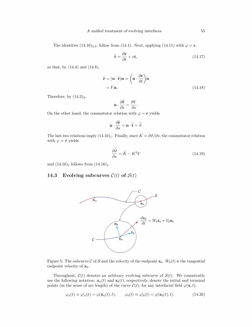
A unified treatment of evolving interfaces 55
The identities (14.16)3,4, follow from (14.1). Next, applying (14.11) with ϕ = r,
!r =∂r∂t
+ vt, (14.17)
so that, by (14.4) and (14.8),
!r = (n · !r)n =(
n · ∂r∂t
)
n
= V n. (14.18)
Therefore, by (14.2)2,
n · ∂!r∂s
=∂V
∂s.
On the other hand, the commutator relation with ϕ = r yields
n · ∂!r∂s
= n ·!t =
!ϑ.
The last two relations imply (14.16)1. Finally, since K = ∂ϑ/∂s, the commutator relationwith ϕ = ϑ yields
∂!ϑ
∂s=
!K − K2V (14.19)
and (14.16)2 follows from (14.16)1.
14.3 Evolving subcurves C(t) of S(t)
xa
SC
xb
xb
dxb
dt= Wbtb + Vbnb
C
nb
tb
Figure 5: The subcurve C of S and the velocity of the endpoint xb. Wb(t) is the tangentialendpoint velocity of xb.
Throughout, C(t) denotes an arbitrary evolving subcurve of S(t). We consistentlyuse the following notation: xa(t) and xb(t), respectively, denote the initial and terminalpoints (in the sense of arc length) of the curve C(t); for any interfacial field ϕ(x, t),
ϕa(t) ≡ ϕ|a(t) = ϕ(xa(t), t), ϕb(t) ≡ ϕ|b(t) = ϕ(xb(t), t). (14.20)

56 E. Fried & M. E. Gurtin
The endpoints of C(t) may also be marked by their arc-length values Sa(t) and Sb(t),where
xa(t) = r(Sa(t), t), xb(t) = r(Sb(t), t), (14.21)
so that, using the arc-length description of ϕ,
ϕa(t) = ϕ(Sa(t), t), ϕb(t) = ϕ(Sb(t), t); (14.22)
henceϕ∣∣b
a≡ ϕb − ϕa =
∫
C
∂ϕ
∂sds.
The functions Wa(t) and Wb(t) defined by
Wa = ta · dxa
dt, Wb = tb ·
dxb
dt
are the tangential endpoint velocities of C(t). Since the normal velocities of the endpointsmust coincide with the normal velocity of S(t),
Va = na · dxa
dt, Vb = nb ·
dxb
dt;
hence (Figure 5)
dxa
dt= Wata + Vana,
dxb
dt= Wbtb + Vbnb. (14.23)
On the other hand, by (14.21),
dxa
dt=∂r∂t
∣∣∣a
+ tadSa
dt,
so that, by (14.22),
dxa
dt= !r∣∣a
+ ta
(dSa
dt− va
)
, (14.24)
and an analogous relation holds for the other endpoint. Thus, since t · !r = 0,
Wa =dSa
dt− va, Wb =
dSb
dt− vb. (14.25)
Given an interfacial field ϕ, the argument leading to (14.24) yields
dϕa
dt= !ϕ∣∣a
+∂ϕ
∂s
∣∣∣∣a
(dSa
dt− va
)
and similarly for the other endpoint. Therefore, by (14.25),
dϕa
dt= !ϕ∣∣a
+∂ϕ
∂s
∣∣∣aWa,
dϕb
dt= !ϕ∣∣b+∂ϕ
∂s
∣∣∣bWb, (14.26)
and applying these relations with ϕ = ϑ yields, since ∂ϑ/∂s = K,
dϑa
dt=
!ϑ∣∣a
+ KaWa,dϑb
dt=
!ϑ∣∣b+ KbWb. (14.27)

A unified treatment of evolving interfaces 57
14.4 Transport theorem for integrals
Let ϕ be an interfacial field. Then
∫
C(t)
ϕ ds =
S2(t)∫
S1(t)
ϕ(s, t) ds.
Thus, writing[
ϕS]b
a= ϕbSb − ϕaSa (14.28)
and suppressing the argument t where convenient, we may use (14.11) to conclude that
d
dt
∫
C(t)
ϕ ds =∫
C
∂ϕ
∂tds +
[
ϕS]b
a=∫
C
(
!ϕ− v
∂ϕ
∂s
)
ds +[
ϕS]b
a.
Thus if we integrate the term v ∂ϕ/∂s by parts and use (14.6) and (14.25), we arrive atthe following theorem (Angenent and Gurtin, 1989):
Transport Theorem for Integrals For C(t) a smoothly evolvingsubcurve of S(t) and ϕ(x, t) a smooth interfacial field,
d
dt
∫
C(t)
ϕ ds =∫
C(t)
( !ϕ− ϕKV ) ds +
[
ϕW]b
a, (14.29)
with
[
ϕW]b
a= ϕbWb − ϕaWa. (14.30)
Notation analogous to (14.30) (for endpoint differences) will be used repeatedly throughoutwhat follows.
15 Deformation of the interface
We now turn to a discussion of deformation. We consider both solid-solid and solid-vaporphase transitions; in the former case we restrict attention to coherent interfaces.
15.1 Interfacial limits
We assume that the interface S(t) separates phases labelled (+) and (−), with the normaln pointing into the (+)-phase. When discussing solid-vapor interfaces, the (+)-phasealways denotes the vapor.
Consider an arbitrary field f(x, t) that is continuous up to S(t) from either side. Let[[f ]] and 〈〈f〉〉 designate the jump and average of f across the interface, while f± denotethe limiting values of f ; specifically, for x on S(t),
[[f ]](x, t) = f+(x, t) − f−(x, t),
〈〈f〉〉(x, t) = 12
(
f+(x, t) + f−(x, t))
,
f±(x, t) = limε→0ε>0
f(x ± εn(x, t), t).
(15.1)

58 E. Fried & M. E. Gurtin
Our discussion of solid-vapor interfaces is limited to situations in which the vapormay, in essence, be represented by the limiting values of its basic fields at the interface;bulk values of these fields away from the interface play no role. In this instance, the fieldf+ simply represents the value of f in the vapor at the interface.
15.2 Interfacial-strain vector
(a) Solid-vapor interface
We assume that the displacement u(x, t) is smooth up to the interface from the solidphase, so that the interfacial strain
e =∂u∂s
= (∇u)t (15.2)
is well defined on S, as is the temporal derivative!u = u + (∇u)v. (15.3)
(b) Coherent solid-solid interface
In our discussion of solid-solid phase transitions we restrict attention to interfaces S thatare coherent in the sense that u is continuous across the interface:35
[[u]] = 0. (15.4)
We do not require that the derivatives of u be continuous across the interface, but wedo require that all such derivatives be continuous up to the interface from either side, anassumption that allows us to compute the interfacial strain
e =∂u∂s
(15.5)
using the limiting values of ∇u on each side of the interface:
e = (∇u)+t = (∇u)−t = 〈〈∇u〉〉t. (15.6)
Similarly, for x = rn(p, t) a normal parametrization of S(t),36 we may use (14.10)and the chain-rule to compute !u as follows:
!u = u+ + (∇u)+v = u− + (∇u)−v = 〈〈u〉〉 + 〈〈∇u〉〉v; (15.7)
this yields the classical compatibility condition
[[u]] + V [[∇u]]n = 0. (15.8)
(c) Identities involving the interfacial strain
It is convenient to introduce the interfacial tensile and shear strains, ε and γ, defined by
e = εt + γn. (15.9)
Then
ε = t · ∂u∂s
, γ = n · ∂u∂s
, (15.10)
35Cf. Cermelli & Gurtin (1994a, b) for discussions of incoherent interfaces.36That is, ∂rn/∂t = V n = v, with ∂/∂t the derivative holding p fixed.

A unified treatment of evolving interfaces 59
so that, using the Frenet formulas (14.2),
∂ε
∂s= t · ∂
2u∂s2
+(
n · ∂u∂s
)
K,∂γ
∂s= n · ∂
2u∂s2
−(
t · ∂u∂s
)
K. (15.11)
Next, the fields u, !u, and e = ∂u/∂s are, for each of the two types of phase transitionsunder consideration, well defined on the interface. We may therefore use the commutatorrelation (14.15) to conclude that
∂!u∂s
= !e − KV e. (15.12)
Let
e = εt + γn; (15.13)
ε and γ, respectively, represent interfacial tensile and shear strains. Then, by (14.16)3,4,the interfacial strain-rate (following the motion of the interface) is given by
!e = (!ε− γ
!ϑ)t + (!
γ + ε!ϑ)n. (15.14)
Thus, interestingly, while the strain ε represents stretching of the interface, the stretchrate, as defined by t · !e, is given by
t · !e = !ε− γ
!ϑ (15.15)
and hence involves the shear strain γ via a term arising from temporal changes in theorientation of the interface.
Let C(t), with endpoints xa(t) and xb(t), be an arbitrary evolving subcurve of S(t),and let
ua(t) = u(xa(t), t) and ub(t) = u(xb(t), t)
denote the corresponding endpoint displacements (see Figure 5), so that
dua
dtand
dub
dt(15.16)
represent motion velocities following these endpoints. Then, by the vectorial counterpartof (14.26),
dua
dt= !u∣∣a
+ eaWa,dub
dt= !u∣∣b+ ebWb. (15.17)
(
These relations may also be derived using the chain-rule and, say (C4):
dua
dt= (u)a + (∇u)a
dxa
dt= (u)a + (∇u)a(Wata + Vana) = !u
∣∣a
+ eaWa, etc.)
16 Interfacial pillboxes
We will discuss interfaces separating grains, solid phases, and solid and vapor phases. Forthe purpose of this discussion, assume that the interface S(t) separates phases labelled(+) and (−), with the normal n pointing into the (+)-phase. Our discussion of configu-rational forces in bulk was based on the use of control volumes that migrate through thebody. The counterpart of this notion for the interface S = S(t) is an interfacial pillbox,which we now define.

60 E. Fried & M. E. Gurtin
SC+
C−
C
xa
xb
(+)-phase
(−)-phase
n
Figure 6: An interfacial pillbox separating (+) and (−) phases.
Consider an arbitrary evolving subcurve C(t) of S(t). Our discusion of basic lawsviews C as a interfacial pillbox of infinitesimal thickness containing a portion of S, a viewthat allows us to isolate the physical processes in the individual phases that interact withS. The geometric boundary of C consists of its endpoints xa and xb. But C viewed aspillbox has a pillbox boundary consisting of (Figure 6):
• a surface C+ with unit normal +n that lies in the (+)-phase;
• a surface C− with unit normal −n that lies in the (−)-phase;
• end faces represented by the endpoints xa and xb of C.
The interaction of C with the bulk phases are then represented by tractions exerted on— and flows of atoms and energy across — the surfaces C+ and C−; the interaction ofC with the remainder of S is represented by forces on — and flows of atoms and energyacross — the endpoints of C.
D Grain boundaries
We here consider a class of theories central to materials science. These theories involveonly configurational forces; deformation and standard forces are neglected.37
17 Simple theory neglecting deformation and atomictransport
We here discuss an evolving grain boundary S = S(t) neglecting deformation and atomictransport.38
37Some workers who utilize the notion of configurational forces do not accept the notion of an inde-pendent configurational force balance, but consider the standard and configurational force balances tobe “projections of a single equation onto two manifolds”. The theories discussed in this part show thatthe configurational balance cannot, in general, be considered as a “projection” of the standard forcebalance, since in these theories there are no standard forces; there are only configurational forces.
38The results of this section are due to Angenent and Gurtin (1989); cf. also Gurtin (1993, 2000).
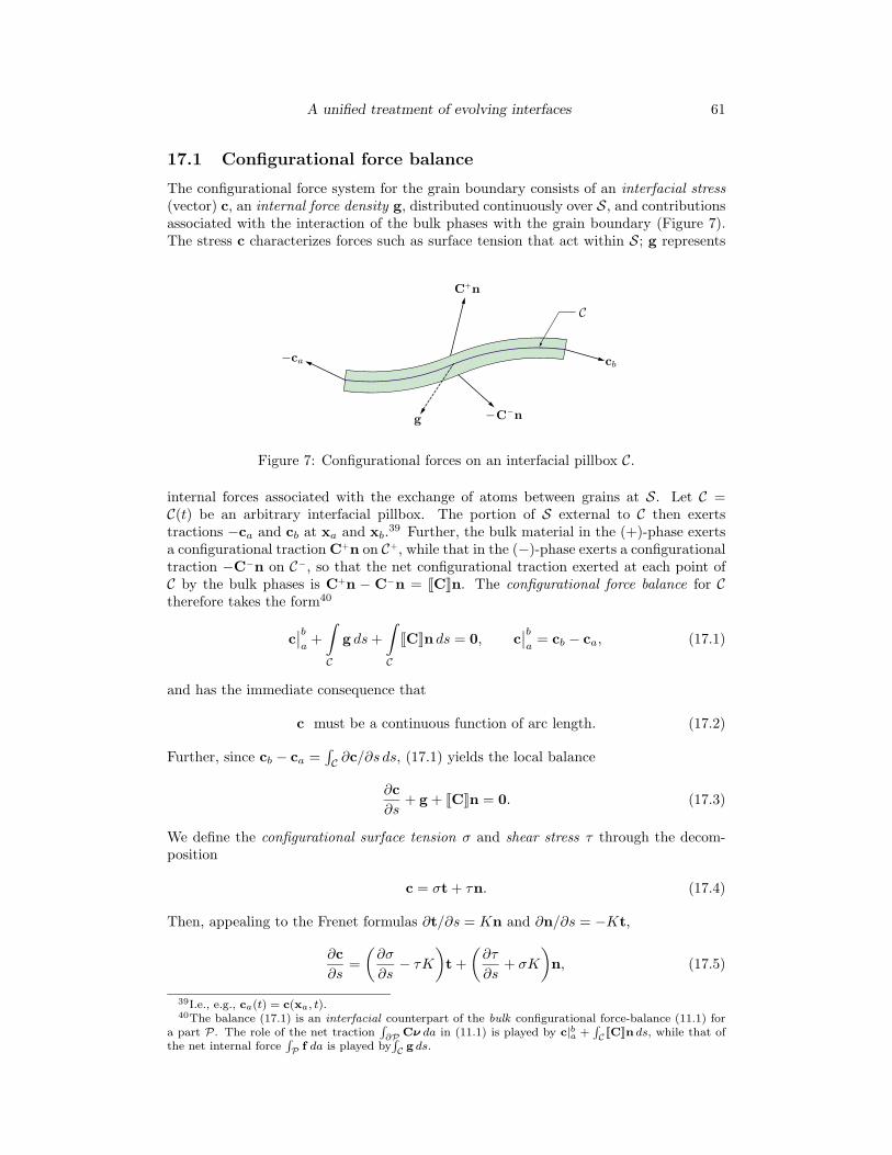
A unified treatment of evolving interfaces 61
17.1 Configurational force balance
The configurational force system for the grain boundary consists of an interfacial stress(vector) c, an internal force density g, distributed continuously over S, and contributionsassociated with the interaction of the bulk phases with the grain boundary (Figure 7).The stress c characterizes forces such as surface tension that act within S; g represents
−
C+n
C−n
−ca
C
g
cb
Figure 7: Configurational forces on an interfacial pillbox C.
internal forces associated with the exchange of atoms between grains at S. Let C =C(t) be an arbitrary interfacial pillbox. The portion of S external to C then exertstractions −ca and cb at xa and xb.39 Further, the bulk material in the (+)-phase exertsa configurational traction C+n on C+, while that in the (−)-phase exerts a configurationaltraction −C−n on C−, so that the net configurational traction exerted at each point ofC by the bulk phases is C+n − C−n = [[C]]n. The configurational force balance for Ctherefore takes the form40
c∣∣b
a+∫
C
g ds +∫
C
[[C]]n ds = 0, c∣∣b
a= cb − ca, (17.1)
and has the immediate consequence that
c must be a continuous function of arc length. (17.2)
Further, since cb − ca =∫
C ∂c/∂s ds, (17.1) yields the local balance
∂c∂s
+ g + [[C]]n = 0. (17.3)
We define the configurational surface tension σ and shear stress τ through the decom-position
c = σt + τn. (17.4)
Then, appealing to the Frenet formulas ∂t/∂s = Kn and ∂n/∂s = −Kt,
∂c∂s
=(∂σ
∂s− τK
)
t +(∂τ
∂s+ σK
)
n, (17.5)
39I.e., e.g., ca(t) = c(xa, t).40The balance (17.1) is an interfacial counterpart of the bulk configurational force-balance (11.1) for
a part P. The role of the net traction∫
∂P Cν da in (11.1) is played by c|ba +∫
C [[C]]n ds, while that ofthe net internal force
∫
P f da is played by∫
C g ds.

62 E. Fried & M. E. Gurtin
whereby the normal component of (17.3), the normal configurational force balance, isgiven by
σK +∂τ
∂s+ g + n · [[C]]n = 0, (17.6)
with
g = g · n (17.7)
the normal internal force. On the other hand, we shall find that g · t is indeterminate,thereby rendering the tangential component of (17.3), namely
∂σ
∂s− τK + g · t + t · [[C]]n = 0, (17.8)
inconconsequential to the theory (cf. the discussion following (17.31)).The bulk configurational stress C is determined by the Eshelby relation (12.15),
which, since we neglect deformation and atomic transport, has the form C = Ψ1, withΨ the bulk free energy; thus
[[C]] = [[Ψ]]1, (17.9)
which we assume to be constant. The normal and tangential components of the configu-rational force balance therefore reduce to
σK +∂τ
∂s+ g + [[Ψ]] = 0 (17.10)
and
∂σ
∂s− τK + g · t = 0. (17.11)
17.2 Power
(a) External expenditure of power
The configurational forces on an interfacial pillbox C are assumed to expend power inconjunction with the migration of the pillbox. The stress c exerts force at the endpointsxa and xb of C, and we therefore take dxa/dt and dxb/dt as the corresponding power-conjugate velocities for c. Analogously, the configurational tractions C+n and −C−nrepresent forces exerted on C+ and C− and are therefore taken to be power-conjugate tothe normal velocity v = V n of C+ and C−. The (net) power expended on C therefore hasthe form
[
c · dxdt
]b
a
+∫
C
[[C]]n · v ds, (17.12)
with[
c · dxdt
]b
a
= cb ·dxb
dt− ca · dxa
dt.

A unified treatment of evolving interfaces 63
(b) Internal expenditure of power. Power balance
By (14.23) and (17.4),
[
c · dxdt
]b
a
=[
σW + τV]b
a, (17.13)
while, by (14.5) and (17.9), [[C]]n · v = [[Ψ]]V ; hence, the power expended on C has theform
[
c · dxdt
]b
a
+∫
C
[[C]]n · v ds =[
σW + τV]b
a+∫
C
[[Ψ]]V ds. (17.14)
Consider the term[
τV]b
a. Using the identity ∂V/∂s = ϑ! (cf. (14.16)1) and the normal
configurational force balance (17.10), it follows that
[
τV]b
a=∫
C
(
τ!ϑ+
∂τ
∂sV)
ds =∫
C
[
τ!ϑ− (σK + g + F )V
]
ds. (17.15)
Combining (17.15) with (17.14) then yields the power balance
[
c · dxdt
]b
a
+∫
C
[[C]]n · v ds
︸ ︷︷ ︸
power expended on C
=[
σW]b
a+∫
C
[
τ!ϑ− (σK + g)V )
]
ds
︸ ︷︷ ︸
power expended within C
. (17.16)
The individual terms comprising the internal power have the following physical interpre-tations (Figure 8):41
• The term[
σW]b
arepresents power expended internally by the surface tension as
material is added to C at its endpoints.
• The term τ!ϑ represents an expenditure of power associated with changes in the
orientation of the grain boundary.
• The term −σKV represents an expenditure of power associated with changes ininterfacial length due to the curvature of the grain boundary.
• The term −gV represents power expended in the exchange of material at the grainboundary; the negative sign signifies that g expends (positive) power when andonly when it opposes motion of the grain boundary.
17.3 Free-energy imbalance
(a) Global imbalance
Guided by the arguments given in §12.4 in support of the free-energy imbalance (12.17)for a migrating control volume in bulk, and bearing in mind that the present theory
41Gurtin (2000, pp. 71, 105). A complete catalog of internal power expenditures is possible only withthe introduction of configurational forces within a structure that embodies the notion of power. Becausethey bypass such fundamental notions, ad hoc methods such as gradient-flow arguments obscure theunderlying physics.

64 E. Fried & M. E. Gurtin
−σKV τ!ϑ − gV σW
Figure 8: Power expenditures within an evolving grain boundary
does not allow for atomic transport, we posit a free-energy imbalance for each interfacialpillbox C(t) in the general form
d
dtfree energy of C(t) ≤ power expended on C(t). (17.17)
As in our treatment of power expended on a migrating control volume, the right sidedoes not account for flows of bulk and interfacial free-energy into the pillbox C(t) acrossits boundaries due to its migration, but it is meant to include power expended on C(t) byconfigurational forces.
Let ψ denote the free energy of the grain boundary, measured per unit length, so that∫
C(t)
ψ(x, t) ds
represents the net free-energy of the interfacial pillbox C(t) at any time t. Thus, bearingin mind the expression (17.12) for the power expended by the configurational forces, wewrite the free-energy imbalance for C in the form
d
dt
∫
C
ψ ds ≤[
c · dxdt
]b
a
+∫
C
[[C]]n · v ds. (17.18)
(b) Growth and decay of an isolated grain
The global free-energy imbalance has interesting consequences. Consider a grain isolatedfrom all other grains, with S the closed curve that represents the grain boundary. Identifythe grain with the (−)-phase, so that the normal n points into the surrounding matrix(Figure 9). Then, since [[C]]n · v = [[Ψ]]V and [[Ψ]] is (assumed) constant,
∫
S(t)
[[Ψ]]V ds = [[Ψ]]A(t),
where A(t) is the area enclosed by S(t) (that is, the area of the grain). Therefore
d
dt
∫
S(t)
ψ ds − [[Ψ]]A(t)
≤ 0, (17.19)
and the quantity in braces decreases with time. If, for example, the bulk free energy ofthe matrix is strictly larger than that of the grain, then [[Ψ]]dA/dt > 0, so that, wereinterfacial energy neglegible, the area of the grain would increase with time, therebylowering the net free energy of the bulk material. On the other hand, assuming thatψ > 0, for [[Ψ]]dA/dt ≤ 0 the area of the grain would decrease with time.

A unified treatment of evolving interfaces 65
S
n
grain
Figure 9: Depiction of an isolated grain.
If the grain and the surrounding matrix have equal free-energy densities, so that[[Ψ]] = 0, then the total free-energy of the grain boundary must decrease with time. If,in addition, the grain-boundary energy ψ > 0 is constant, then
d
dt
length of S(t)
≤ 0
and the grain boundary must shorten with time.
(c) Indeterminacy of the tangential component of the internal force g
Note that there is no expenditure of power associated with “tangential motion” of thegrain boundary S (which is to be expected, since only the normal motion of S is intrinsic).Consistent with a “constraint” of this type, we leave as indeterminate the tangentialcomponent g · t of the internal force. This assumption renders the tangential balance(17.8) irrelevant and allows us to restrict attention to the normal configurational forcebalance (17.10). This will be the case throughout what follows; for that reason, we willoften leave the tangential configurational force balance unmentioned (cf. Remark 6 onpage 6).
(d) Equality of surface tension and interfacial free energy
In view of the transport theorem (14.29) and the power balance (17.16), the free-energyimbalance for C, namely (17.18), becomes
∫
C
(!ψ − ψKV ) ds +
(#)︷ ︸︸ ︷[
(ψ − σ)W]b
a≤∫
C
[
τ!ϑ− (σK + g)V
]
ds. (17.20)
Since C is arbitrary, so also are the tangential velocities Wa and Wb of the endpoints ofC; since the only term in (17.20) dependent on these velocities is the term (#), it followsthat
σ = ψ. (17.21)
66 E. Fried & M. E. Gurtin
There are many misconceptions concerning the relation between surface tension andinterfacial free energy. Here surface tension enters the theory via a force balance, whereasfree-energy enters via an energy imbalance; the fact that they coalesce is a consequenceof the theory. As we shall see, in more general theories allowing for interfacial torques,standard interfacial stress, or atomic transport accounting for atomic densities within theinterface, the relation σ = ψ is no longer valid.
Note that, by (17.21), we may rewrite the normal configurational force balance (17.10)as
ψK +∂τ
∂s+ g + [[Ψ]] = 0. (17.22)
(e) Dissipation inequality
By (17.21), the free-energy inequality (17.20) reduces to∫
C
(!ψ − τ
!ϑ+ gV ) ds ≤ 0;
since C is arbitrary, we have the dissipation inequality
!ψ − τ
!ϑ+ gV ≤ 0. (17.23)
17.4 Constitutive equations
As in our discussion of bulk behavior, we use the dissipation inequality (17.23) as aguide in the development of constitutive equations for the grain boundary. Moreover, werequire that the local dissipation inequality hold in all “processes” related through theconstitutive equations.
(a) Basic constitutive equations. Restrictions.
It would seem clear from the dissipation inequality (17.23) that, at bottom:
• ψ and τ should depend on ϑ, an assumption common to more classical theories(cf., e.g., Herring (1951));
• g should depend on V and, since classical theories display linear kinetics (cf., e.g.,Mullins (1956)), this dependence might be linear; anisotropy would require a de-pendence of g also on ϑ.
We therefore begin with constitutive equations
ψ = ψ(ϑ),
τ = τ(ϑ),
g = −b(ϑ)V.
(17.24)
Here b(ϑ) is a kinetic modulus associated with the attachment kinetics of atoms at thegrain boundary.
By the chain rule (14.12),
!ψ =
dψ(ϑ)dϑ
!ϑ, (17.25)

A unified treatment of evolving interfaces 67
and since the constitutive relations (17.24) are independent of V , we may conclude, upontaking V = 0 in the dissipation inequality (17.23), that ψ! −τϑ! ≤ 0. Thus compatibilitywith (17.23) requires that
dψ(ϑ)
dϑ− τ(ϑ)
!ϑ ≤ 0 (17.26)
for all choices of the orientation field ϑ. We may therefore restrict attention to spatiallyuniform functions ϑ(t), so that ϑ! = ϑ. Given any choice of the time t0, we can alwaysfind a choice of ϑ(t) such that ϑ(t0) and ϑ(t0) take on arbitrarily prescribed values. Thus,since ϑ! appears linearly in (17.26), its coefficient must vanish: τ = ∂ψ/∂ϑ. The freeenergy must therefore determine the configurational shear through the relation
τ =dψ(ϑ)
dϑ. (17.27)
Finally, by (17.27), the dissipation inequality reduces to gV ≤ 0, which renders
b(ϑ) ≥ 0. (17.28)
(b) Remarks
1. Anisotropy of the interface manifests itself in a nontrivial dependence of ψ(ϑ) on ϑ.An interesting and important consequence of (17.27) is that, for a grain boundarywith anisotropic free energy, the surface shear cannot vanish.42
2. By (17.4), (17.21), and (17.27), we may consider the configurational stress c as afunction c = c(ϑ), with
c(ϑ) = ψ(ϑ)t(ϑ) +dψ(ϑ)
dϑn(ϑ). (17.29)
3. The normal internal force g is a dissipative force associated with the rearrangementof atoms at the grain boundary. The term
D def= −gV = b(ϑ)V 2
represents the dissipation per unit length of the interface, as its integral over Crepresents the right side of the free-energy imbalance (17.17) (the expended power)minus its left side (the net rate of change of free-energy); this dissipation is char-acterized by the kinetic modulus b(ϑ).
4. Were we to begin with constitutive relations of the form
ψ = ψ(ϑ, V ),
τ = τ(ϑ, V ),
g = g(ϑ, V ),
(17.30)
thereby satisfying equipresence, the dissipation inequality would render ψ and τindependent of V and consistent with (17.27), and would yield the reduced dissipa-tion inequality g(ϑ, V ) ≤ 0; then, as in the discussion leading to (17.24)3, linearityof g = g(ϑ, V ) in V would require an additional hypothesis.
42Cf. Angenent and Gurtin (1989, eqt. 4.2), although this result is clear from the work of Herring(1951) in his discussion of the equilibrium theory within a variational framework.

68 E. Fried & M. E. Gurtin
5. More general constitutive equations are also possible. For example, a constitutiverelation of the form
τ =dψ(ϑ)
dϑ− C(ϑ)
!ϑ, C(ϑ) > 0
would be consisitent with the dissipation inequality.
6. Since, by (17.21) and (17.27), σ = ψ and τ = ψ′(ϑ),
∂σ
∂s= τ
∂ϑ
∂s= τK,
and we may conclude from the tangential configurational balance (17.8) that
g · t = 0. (17.31)
Thus the tangential component of the internal force g vanishes. This result is aconsequence of the special theory under consideration; as we shall see, for theoriesthat account for the density of atoms within the interface the tangential force g ·t isneeded to balance spatial inhomogeneities on the interface induced by variations inchemical potential (cf. (13.4) and the discussion following (17.8)). For the theoriesdiscussed in §18 and §19, which account, respectively, for configurational torquesand the diffusion of a single atomic species, it is also the case that g · t = 0.
17.5 Evolution equation for the grain boundary. Parabolicityand backward parabolicity
We now return to our discussion of grain boundaries as described by the constitutiveequations
τ =dψ(ϑ)
dϑ, g = −b(ϑ)V,
assuming that b(ϑ) > 0.For any function f(ϑ) we write
f ′(ϑ) =df(ϑ)dϑ
,
and, when there is no danger of confusion, we write
ψ(ϑ) = ψ(ϑ).
Then, since K = ∂ϑ/∂s, (17.27) yields ∂τ/∂s = ψ′′(ϑ)K; thus, by (17.24)3, the normalconfigurational force balance reduces to the curvature-flow equation43
b(ϑ)V =[
ψ(ϑ) + ψ′′(ϑ)]
K + [[Ψ]]. (17.32)
Note that the larger the dissipation, as characterized by the modulus b(ϑ), the slowerthe motion of the interface.
43Proposed by Uwaha (1987, eqt. 2) and independently by Gurtin (1988, eqt. 8.3). Cf. also Angenentand Gurtin (1989). Evolution according to (17.32) is studied by Angenent (1991), Chen, Giga, andGoto (1991), Barles, Soner, and Souganides (1993), and Soner (1993). A formulation of (17.32) using avariational definition of the curvature term is given by Taylor, Cahn, and Handwerker (1992), who giveextensive references. The term ψ(ϑ) + ψ′′(ϑ) appears first in the study of Herring (1951), who showsthat it represents the variational derivative of the net interfacial free-energy with respect to variationsin the position of the interface.

A unified treatment of evolving interfaces 69
y
x
ϑ St
y = h(x, t)
Figure 10: Sign conventions when the interface is a graph y = h(x, t).
For an isotropic grain boundary both b and ψ are positive constants. Then, for[[Ψ]] = 0 and, with an appropriate rescaling of space and time, (17.32) has the simple(and beautiful) form
V = K,
a parabolic partial differential equation with a large literature.44 This equation, whichwas the forerunner of (17.32), was introduced by Burke and Turnbull (1952) and Mullins(1956) to study the motion of grain boundaries.
Locally the interface may be represented as the graph of a function y = h(x, t),provided the x and y axes are chosen appropriately. Consider the choice indicated inFigure 10 (with orientation such that arc length increases with increasing x) and let
q =∂h
∂x.
Then, for −π2 < ϑ < π
2 ,
q = tanϑ, K =1
(1 + q2) 32
∂2h
∂x2, V =
1√
1 + q2
∂h
∂t, (17.33)
and, assuming that b(ϑ) > 0 for all such ϑ, we may use these relations to rewrite theevolution equation (17.32) in the form
∂h
∂t= A(q)
∂2h
∂x2+ P (q), (17.34)
with
A(q) =ψ(ϑ) + ψ′′(ϑ)
b(ϑ) cosϑ (1 + tan2 ϑ) 32,
P (q) =F
b(ϑ) cosϑ, q = tanϑ.
For the angle range −π2 < ϑ < π
2 under consideration, sgnA(q) = sgn [ψ(ϑ) + ψ′′(ϑ)]
.Thus the evolution equation ((17.34) and hence) (17.32) is:45
44Cf. Gurtin (2000) for references.45Angenent and Gurtin (1989).

70 E. Fried & M. E. Gurtin
(i) parabolic on any angle interval over which ψ(ϑ) + ψ′′(ϑ) > 0;
(ii) backward parabolic (and hence unstable as a partial differential equation) on anyangle interval over which ψ(ϑ) + ψ′′(ϑ) < 0.
Let
φ(ϑ) def= ψ(ϑ) + ψ′′(ϑ). (17.35)
Materials scientists often refer to φ(ϑ) as the interfacial stiffness. When φ(ϑ) > 0 forall ϑ, (17.32), being parabolic, exhibits behavior that is not much different than that forV = K, and is well understood.46 What makes (17.32) nonstandard is the possibilityof backward parabolicity for interfacial free-energy densities that satisfy φ(ϑ) < 0 forcertain angle-intervals. Such energy densities are not mathematical curiosities: materialsscientists give strong arguments in support of free-energy densities with φ(ϑ) < 0 forsome angles ϑ.47
17.6 Backward parabolicity. Facets and wrinklings
In analyzing energies with backward-parabolic angle-intervals an important concept is theFrank diagram F ,48 which is the graph in polar coordinates of the function r = 1/ψ(ϑ):F is locally strictly convex where φ(ϑ) > 0 and locally strictly concave where φ(ϑ) < 0.One method of dealing with the backward-parabolic intervals is to allow the interface tocontain corners (jumps in tangent angle) that exclude the backward-parabolic ranges of ϑ.In the presence of a corner, the evolution equation (17.32) does not by itself characterizethe motion of the interface; there is an additional condition (17.2) requiring that theconfigurational stress
c(ϑ) = ψ(ϑ)t(ϑ) +dψ(ϑ)
dϑn(ϑ) be a continuous function of arc length
(cf. (17.29)). Thus for a corner corresponding to an angle jump from ϑ1 to ϑ2 we musthave
c(ϑ1) = c(ϑ2),
a condition that has important consequences. One can show that: (i) the tangent lineto F at ϑ1 must also be a tangent line to F at ϑ2 (that is, ϑ1 and ϑ2 must be anglesof bitangency for F); and (ii) there is exactly one (maximal) angle interval between ϑ1
and ϑ2 on which φ(ϑ) < 0. Thus, by restricting attention to an interface with cornerssuch that there is one corner for each backward parabolic interval and such that acrosseach corner the tangent angle jumps between bitangency angles of the Frank diagram, onearrives at an interface whose evolution is governed by a parabolic equation (Angenent andGurtin, 1993). This procedure leads to to a free-boundary problem, since the positionsof the corners vary with time.
The presence of unstable angle-intervals allows for facets (flat sections) and wrinklings,which are interfacial sections consisting of facets whose tangent angle is ϑ1 alternatingwith facets whose tangent angle is ϑ2 (Figure 11). Because K ≡ 0 on each facet, facetswith tangent angle ϑ1 must, by (17.32), have constant normal velocity V ≡ V1 = F/b(ϑ1),while V ≡ V2 = F/b(ϑ2) for those with angle ϑ2. Then, by compatibility, the wrinklingmust evolve as a rigid body with velocity w defined by w · n(ϑi) = F/b(ϑi), i = 1, 2.49
46Cf. Angenent (1991), Chen, Giga, and Goto (1991), Barles, Soner, and Souganides (1993), and Soner(1993)
47Cf. Gjostein (1963) and Cahn and Hoffman (1974).48Frank (1963).49Cf. Gurtin (1993, §11) for a thorough discussion of wrinklings and related phenomena.

A unified treatment of evolving interfaces 71
t1
t2C
Figure 11: A wrinkled portion C of the grain boundary S. The angles ϑ1 and ϑ2 associatedwith the facet-tangents t1 and t2 must be bitangency angles of the Frank diagram.
17.7 Junctions
S1
S2
S3
c1
c2
c3
Figure 12: A triple-junction with a corresponding junction pillbox. Only the interfacialtractions on the pillbox are shown.
In the two-dimensional theory under consideration, grain boundaries meet at junc-tions such as the one shown in Figure 12. This figure shows the pillbox used to determinethe configurational force balance for the junction; this figure omits the forces exerted bythe bulk material on the pillbox as well as the internal forces exerted on the grain bound-aries; we assume that these forces approach zero as the pillbox collapses to the junction.For the case in which N grain boundaries, labelled n = 1, 2, . . . , N , meet at a junc-tion, and for which the individual grain boundaries are oriented so that the unit tangentfield of each is directed away from the junction, the configurational force balance for thejunction has the form
N∑
n=1
cn + net force exerted on the pillbox by the bulk material
+ net internal force exerted on the pillbox = 0, (17.36)
where cn denotes the force exerted on the pillbox by the portion of grain-boundary nthat lies outside the pillbox. Assuming that the two terms written . . . tend to zero as

72 E. Fried & M. E. Gurtin
the pillbox tends to the junction, we arrive at Herring’s junction balance (1951):50
N∑
n=1
cn = 0, (17.37)
or, equivalently,N∑
n=1
(σntn + τnnn) = 0.
A classical consequence of the junction balance is that, for a triple junction, if the freeenergies of the grain boundaries are constant and equal, then the angles between adjacentboundaries are equal, with 2π
3 the common angle.
17.8 Digression: general theory of interfacial constitutive rela-tions with essentially linear dissipative response
In our development of constitutive equations for grain-boundaries, we used the dissipa-tion inequality ψ! − τϑ! + gV ≤ 0 (and experience with classical theories) to motivateconstitutive relations giving ψ and τ as functions of ϑ together with a relation giving gas a function of ϑ and V . This procedure will be used repeatedly in this article, whereeach of the individual theories is based on a dissipation inequality of the form
!ψ −
N∑
m=1
τn!ϑn +
N∑
m=1
gmVm ≤ 0. (17.38)
In these theories we use the terms
!ψ −
N∑
m=1
τn!ϑn,
N∑
m=1
gmVm,
respectively, to motivate constitutive relations giving51
ψ, +τ as functions of +ϑ , +g as a function of (+ϑ, +V ), (17.39)
50In describing the forces on the junction, we neglected the internal configurational force g∗ on thejunction, which if included would appear on the left side of (17.37). If we neglect junction energy, thenthe appropriate free-energy imbalance for the junction would lead to the inequality g∗ · v∗ ≤ 0, wherev∗ is the junction velocity. In this manner we would be led to a constitutive equation
g∗ = −Bv∗
with B a positive semi-definite tensorial modulus that may depend on the junction angles of the grainboundaries as well as the mismatch angles of the grains. In this manner, we would arrive at the balance∑
n cn = Bv∗. Cf. Simha and Bhattacharya (1998); Gurtin (2000, Part H); cf. also Suo (1997, eqt.(2.17)), whose analysis is restricted to isotropic surface energies and to a junction between two grainsand a vapor, a situation of great interest in discussing grain-boundary grooving (cf. Mullins (1957)).
51This structure cannot include theories involving temporal derivatives (or past histories) of the inde-pendent constitutive variables, nor can it include theories whose constitutive equations involve variablesnot present in the dissipation inequality. But it does include constitutive theories that we believe to beappropriate for the class of applications under consideration, without encumbering the presentation withlengthy arguments involving thermodynamical reductions of general constitutive theories. Moreover, asis clear from Remark C.1 above, the a priori splitting presumed in (17.39), in which ψ and %τ are taken
to be independent of %V , may, in come cases, be unnecessary (e.g., in §18). But in discussions involving
surface diffusion, spatial derivatives of chemical potentials enter the list %V .

A unified treatment of evolving interfaces 73
where
+τ = (τ1, τ2, . . . , τN ),
+g = (g1, g2, . . . , gM ),
+ϑ = (ϑ1,ϑ2, . . . ,ϑN ),
+V = (V1, V2, . . . , VM ).
and where neither of the fields +ϑ and +V involves temporal derivatives of the other.In view of the chain-rule (14.12), thermodynamic compatibility requires that, for any
choice of the fields +ϑ and +V ,
N∑
n=1
∂ψ(+ϑ)∂ϑn
− τn(+ϑ )
!ϑn +
M∑
m=1
gm(+ϑ, +V )Vm ≤ 0. (17.40)
It is always possible to find an interfacial field +ϑ whose values and whose (normal) time-derivative-values at any given time are arbitrary. Thus, since the inequality (17.40) islinear in the variables ϑ!
n, we must have τn = ∂ψ/∂ϑn (for all n). We therefore have thefollowing thermodynamic restrictions:
• ψ must determine +τ through the relations
τn =∂ψ(+ϑ )∂ϑn
; (17.41)
• the constitutive response function for +g must be consistent with the reduced dissi-pation inequality
M∑
m=1
gm(+ϑ, +V )Vm ≤ 0. (17.42)
In the special cases we shall consider,
D def= −M∑
m=1
gm(+ϑ, +V )Vm
represents the dissipation. Of special interest here are constitutive equations giving +g asa linear function of +V for each fixed value of +ϑ:
gm = −M∑
j=1
Amj(+ϑ )Vj ; (17.43)
in this case we refer to the constitutive equations as having essentially linear dissipativeresponse. (The term “essential” refers to the fact that (17.43) is linear in the primaryvariable +V , but the dependence on +ϑ is unrestricted). In addition, if
Amj = 0 for m )= j, (17.44)
so that, writing Am = Amm,
g1 = A1(+ϑ )V1,
g2 = A2(+ϑ )V2,
...
gN = AN (+ϑ )VN ,
(17.45)

74 E. Fried & M. E. Gurtin
we refer to the constitutive equations as having uncoupled essentially linear dissipativeresponse.
Returning to the uncoupled relations (17.42), the reduced dissipation inequality re-quires that the coefficients Amj(+ϑ ) form a positive semi-definite matrix. The dissipationcorresponding to the constitutive relations (17.43) has the form
D =M∑
m,j=1
Amj(+ϑ )VmVj . (17.46)
18 Interfacial couples. Allowance for an energetic de-pendence on curvature
Within the theory for grain boundaries presented above, facets are modeled as sharpcorners. That crystalline solids may exhibit departures from this idealization was recog-nized by Herring (1951),52 who argued that, when the radius of curvature of a crystalsurface is sufficiently small, the free energy of that surface should depend not only onorientation but also on curvature. A theory which allows for such dependence has nu-merous benefits. The procedure discussed in §17.6 cannot, by itself, characterize thenucleation of facets and wrinklings, nor can it be used for an initial-value problem inwhich the initial interface has angle intervals for which ψ(ϑ) + ψ′′(ϑ) < 0. To analyzebehavior within such angle-intervals, a regularization of the evolution equation (17.32)is needed. Such a regularization, proposed by Angenent and Gurtin (1989) and devel-oped by DiCarlo, Gurtin, and Podio-Guidugli (1992),53 entails a curvature-dependentfree energy. Within the present framework, a curvature-dependent free energy requires(configurational) interfacial couples together with a configurational balance for torques.A theory including these ingredients provides a physically-based regularization of the evo-lution equation (17.32), in contrast to the pragmatic alternative of simply adding to suchan equation supplemental terms involving higher-order derivatives.
18.1 Configurational torque balance
We now expand the configurational force system discussed in Section §17.1 to include a(scalar) interfacial couple-stress M and a (scalar) internal couple m distributed continu-ously over S (Figure 13). Let C = C(t) be an arbitrary interfacial pillbox S. The portionof S external to C then exerts torques −Ma − (xa − 0)×ca and Mb(xb − 0)×cb at xa
and xb.54 In addition to the interfacial couple m distributed uniformly over C, there isthe torque (x− 0)×g associated with the internal force g. Further, the bulk material inthe (+)-phase exerts a torque (x − 0)×C+n on C+, while that in the (−)-phase exerts atorque −(x−0)×C−n on C−, so that the net configurational torque exerted at each pointof C by the bulk phases is (x − 0)×(C+n − C−n) = (x − 0)×[[C]]n. The configurational
52Cf., also, Gjostein (1963) and Cahn and Hoffman (1974).53Cf. Stewart and Goldenfeld (1992), who define the chemical potential as the variational derivative
of the interfacial energy with respect to changes in the location of the surface and, starting with amass balance that includes surface diffusion and evaporation terms, derive an evolution equation which,after linearization, yields conditions for the onset of instabilities (and the subsequent formation of facetsalong the surface). Cf. also Golovin, Davis, and Nepomnyashchy (1998, 1999), who use variationalarguments to obtain an evolution equation for an interface z = h(x, t) (respectively, z = h(x, y, t)) witha curvature-dependent surface tension, assuming that dh/dx is small (respectively, ∂h/∂x and ∂h/∂yare small).
54Here the “×” denotes the (scalar) two-dimensional cross-product; in components p×k = p1k2−p2k1.

A unified treatment of evolving interfaces 75
−Ma
Mb
mC
Figure 13: Configurational couples on on an interfacial pillbox C. In the configurationaltorque balance these couples are supplemented by torques exerted by the configurationalforce system.
torque balance for C therefore takes the form
[
M + (x − 0)×c]b
a+∫
C
m ds +∫
C
[
(x − 0)×(g + [[C]]n)]
ds = 0. (18.1)
This balance supplements the configurational force balance (17.1).Consider the term
[
M +(x−0)×c]b
a. Since ∂x/∂s = t, and since, by (17.4), t×c = τ ,
[
M + (x − 0)×c]b
a=∫
C
(∂M
∂s+ τ + (x − 0)× ∂c
∂s
)
ds.
Thus, by the local consequence (17.3), namely ∂c/∂s + g + [[C]]n = 0, of the configura-tional force balance (17.1), the torque balance (18.1) reads
∫
C
(∂M
∂s+ m + τ
)
ds = 0;
since C is arbitrary, this yields the local torque balance
∂M
∂s+ m + τ = 0. (18.2)
Differentiating each term of (18.2) with respect to s and using the normal configurationalforce balance (17.6) to give an expression for ∂τ/∂s, it follows that
∂2M
∂s2+∂m
∂s− σK − g − n · [[C]]n = 0, (18.3)
or equivalently, granted C = Ψ1 as in the theory without couples, that
∂2M
∂s2+∂m
∂s− σK − g − [[Ψ]] = 0, (18.4)
with [[Ψ]] assumed constant. This balance is basic to what follows.
18.2 Power
(a) External expenditure of power
Let C = C(t) be an interfacial pillbox. In addition to the power expended by configu-rational forces, we must now account for power expended by the couple stress M . This

76 E. Fried & M. E. Gurtin
stress acts at the endpoints of C and the corresponding torques Ma and Mb should bepower-conjugate to the angle-rates dϑa/dt and dϑb/dt at these endpoints (cf. (14.22)).Thus
[
Mdϑ
dt
]b
a
≡ Mbdϑb
dt− Ma
dϑa
dt
represents the power expended on C by the couple stress, and the (net) power expendedon C has the form
[
c · dxdt
+ Mdϑ
dt
]b
a
+∫
C
[[C]]n · v ds. (18.5)
By (14.27),
[
Mdϑ
dt
]b
a
=[
M(!ϑ+ KW )
]b
a, (18.6)
so that, using (14.19),
[
Mdϑ
dt
]b
a
=[
MKW]b
a+∫
C
(
M∂
!ϑ
∂s+∂M
∂s
!ϑ
)
ds
=[
MKW]b
a+∫
C
(
M(!K − K2V ) +
∂M
∂s
!ϑ
)
ds.
On the other hand, (17.16) (which holds here also) and (18.2) yield
[
c · dxdt
]b
a
+∫
C
[[C]]n · v ds =[
σW]b
a+∫
C(t)
[
τ!ϑ− (σK + g)V
]
ds
=[
σW]b
a−∫
C
(
(σK + g)V +(∂M
∂s+ m
)!ϑ
)
ds.
Adding the last two relations, we arrive at the power balance
[
c · dxdt
+ Mdϑ
dt
]b
a
+∫
C
[[C]]n · v ds
=[
(σ + MK)W]b
a+∫
C
[
M!K − m
!ϑ−(
(σ + MK)K + g)V]
ds, (18.7)
which bears comparison to (17.16). Note that here:
• The term[
(σ + MK)W]b
a(rather than
[
σW]b
a) represents power expended inter-
nally as material is added to C at its endpoints.
• The term M!K represents an expenditure of power associated with changes in the
curvature of the grain boundary.
• The term −m!ϑ (rather than τ
!ϑ ) represents the expenditure of power associated
with changes in the orientation of the grain boundary.

A unified treatment of evolving interfaces 77
• The term −(σ + MK)KV (rather than −σKV ) represents the expenditure ofpower associated with changes in interfacial area due to the curvature of the grainboundary.
As before, the tangential component of g expends no power internally, but now,interestingly, neither does the shear τ , as its role in the power balance is replaced by theinternal torque m. This is consistent with the theory without couples, since, by (18.2),τ = −m when M = 0. Classically, forces that expend no power internally are presumedto be indeterminate; for that reason, τ joins g ·t as an indeterminate field, an assumptionthat allows us to consider the torque balance (18.2) as a defining relation for τ . Notethat, granted τ is defined by the torque balance, the balance (18.4) is equivalent to thenormal configurational force balance (17.10) of the theory without couples.
18.3 Free-energy imbalance
(a) Global imbalance
As before, we let ψ denote the free energy of the grain boundary; the free-energy imbalancefor C then takes the form
d
dt
∫
C(t)
ψ ds ≤[
c · dxdt
+ Mdϑ
dt
]b
a
+∫
C(t)
[[C]]n · v ds. (18.8)
Note that, since [[C]]n · v = [[Ψ]]V , with [[Ψ]] (assumed) constant, the decay relation(17.19) and its consequences remain valid within this more general theory.
(b) Dissipation inequality
In view of the transport identity (14.29) and the power balance (18.7), the free-energyinequality (18.8) becomes
∫
C
(!ψ − ψKV ) ds +
(#)︷ ︸︸ ︷[(
ψ − (σ + MK))
W]b
a
≤∫
C
[
M!K − m
!ϑ−(
(σ + MK)K + g)
V]
ds. (18.9)
Since C is arbitrary, so also are the tangential velocities Wa and Wb of the endpoints ofC; thus, since the only term in (18.9) dependent on these velocities is the term (#), wehave the relation
σ = ψ − MK; (18.10)
thus, in contrast to classical theories, the present theory requires that the correspondencebetween surface tension and interfacial free energy be generalized to account for theinfluence of the interfacial couple-stress M . Using (18.10), we may rewrite the normalconfigurational force balance (17.10) as
(ψ − MK)K +∂τ
∂s+ g + [[Ψ]] = 0. (18.11)

78 E. Fried & M. E. Gurtin
Next, by (18.10), the free-energy inequality (18.9) reduces to∫
C
(!ψ + m
!ϑ− M
!K + gV ) ds ≤ 0, (18.12)
and this yields the dissipation inequality
!ψ + m
!ϑ− M
!K + gV ≤ 0. (18.13)
18.4 Constitutive equations
Guided by (18.13) and the discussion of §17.4 for the theory without configurationalmoments, we consider constitutive equations giving
ψ, m, M as functions of (ϑ, K),
g as a function of (ϑ, K, V ).
(18.14)
Then, appealing to the general constitutive theory discussed in §17.8, we find, as aconsequence of thermocompatibility and an assumption of essentially linear dissipativeresponse, that:
• the free energy determines the internal couple and the interfacial couple-stressthrough the relations
m = −∂ψ(ϑ, K)∂ϑ
,
M =∂ψ(ϑ, K)∂K
.
(18.15)
• the normal internal force is given by the linear relation
g = −b(ϑ, K)V, (18.16)
with kinetic modulus b(ϑ, K) ≥ 0.
18.5 Evolution equation for the grain boundary
The basic equations of the theory consist of the balance (18.4) with σ = ψ − MK, viz.,
∂2M
∂s2+∂m
∂s− (ψ − MK)K − g − [[Ψ]] = 0, (18.17)
supplemented by the constitutive relations (18.15) and (18.16). In general, the couplingbetween orientation and curvature induced by the constitutive relation for the free en-ergy renders the resulting evolution complicated. But, for small curvatures, a quadraticdependence on curvature should provide a reasonable approximation and, as we shall see,such an energy provides a parabolic regularization to the evolution equation (17.32).
We therefore consider the simple constitutive equation
ψ(ϑ, K) = ψ0(ϑ) + 12λK2, (18.18)
with λ > 0 constant. The restrictions (18.15) then yield the specific relations
m = −ψ′0(ϑ), M = λK;

A unified treatment of evolving interfaces 79
thus, assuming that b = b(ϑ) > 0, (18.16) and (18.17) yield the evolution equation
b(ϑ)V =[
ψ0(ϑ) + ψ′′0 (ϑ)]
K − λ
(∂2K
∂s2+ 1
2K3
)
+ [[Ψ]]. (18.19)
For the interface a graph y = h(x, t), we can use (17.33) to rewrite the evolutionequation (18.19) in a form analogous to (17.34). The right side of the resulting equationthen contains a term of the form
−(. . . )∂4h
∂x4,
and all other terms as well as the coefficient ( . . . ) depend on partial derivatives of h withrespect to x of order strictly less than four. Moreover, the coefficient ( . . . ) is strictlypositive. Thus the evolution equation (18.19) is equivalent to a fourth-order parabolicpartial differential equation. In that sense, (18.19) with λ small represents a parabolicregularization of the evolution equation (17.32). This regularization should be useful inanalyzing situations for which the interfacial stiffness is negative and (17.32) is backwardparabolic for certain angle intervals.
In a sense, the regularized equation (18.19) represents a counterpart for interfaces ofthe classical Cahn-Hilliard equation (Cahn and Hilliard, 1958, 1959, 1971), as discussedby DiCarlo, Gurtin, and Podio-Guidugli (1992).55
19 Grain-vapor interfaces with atomic transport
In this section we consider an interface S = S(t) that separates a grain from a vaporenvironment. We include atomic transport in bulk, on the interface, and from the vapor,but neglect deformation of the grain and flow in the vapor.56 For simplicity, we restrictattention to a single atomic species. We model the vapor as a reservoir whose sole inter-action with the grain is through the evaporation of atoms from — and the condensationof atoms on — the grain boundary.
19.1 Configurational force balance
We assume that the configurational stress in the vapor vanishes:57 considering the vaporto be the (+)-phase, the grain the (−)-phase, it follows that C+ = 0.
Apart from this restriction, the discussion of configurational forces is identical to thatpresented for a grain-grain interface. Thus, writing C = C−, the configurational forcebalance (17.1) takes the form
c∣∣b
a+∫
C
g ds −∫
C
Cn ds = 0, (19.1)
55Cf. Watson, Otto, Rubinstein and Davis (2003) and Watson (2003).56Cf. Spencer, Voorhees, and Davis (1991, 1993), Spencer and Meiron (1994), Guyer and Voorhees
(1996, 1998), and Spencer, Voorhees, and Tersoff (2000), who investigate the morphological stabilityof epitaxially strained single-component and alloy thin films in the presence of surface diffusion andan isotropic surface free-energy. See also Zhang and Bower (1999, 2001), who examine shape changesof strained islands on lattice-mismatched substrates due to surface diffusion in the presence of bothisotropic and anisotropic surface energies.
57Tacit are the following assumptions: the free energy of the grain is reckoned relative to that of thevapor; the atomic density of the vapor and the vapor pressure are negligible.

80 E. Fried & M. E. Gurtin
and this yields the normal configurational force balance
σK +∂τ
∂s+ g − n · Cn = 0, (19.2)
with σ and τ defined by (17.4) and g = g · n, as before.The bulk configurational force C is determined by the Eshelby relation (12.15), which,
since deformation is neglected here, has the form
C = (Ψ− ρµ)1, (19.3)
with µ, the bulk chemical-potential, assumed continuous up to the grain boundary. Thenormal configurational force balance (19.1) therefore takes the form
ρµ = Ψ− σK − ∂τ
∂s− g (19.4)
and the normal configurational force balance provides a relation for the chemical potentialof the grain boundary. Finally, the tangential component of the configurational forcebalance reduces to (17.11).
19.2 Power
Consistent with the requirement that the configurational stress vanishes in the vapor andthe notational convention C = C−, the (net) power expended on a migrating pillbox Chas the form
[
c · dxdt
]b
a
−∫
C
Cn · v ds. (19.5)
By (17.13), (14.5), and the Eshelby relation (19.3), Cn · v = (Ψ − ρµ)V ; hence, thepower expended on C has the form
[
c · dxdt
]b
a
−∫
C
Cn · v ds =[
σW + τV]b
a−∫
C
(Ψ− ρµ)V ds (19.6)
which, by (17.15) and the normal configurational force balance (19.4), yields the powerbalance
[
c · dxdt
]b
a
−∫
C
Cn · v ds =[
σW]b
a+∫
C
[
τ!ϑ− (σK + g)V )
]
ds. (19.7)
19.3 Atomic flows due to diffusion, evaporation-condensation,and accretion. Atomic balance
In addition to the bulk atomic density ρ and bulk atomic flux , we account for an atomicsupply r from the vapor and for a (scalar) interfacial atomic flux58 h. Without loss ofgenerality, we write ρ = ρ− and = − for the interfacial limits of the density and atomicflux in the grain. While we account for the transport of adatoms along the interfacethrough the flux h, we assume that the adatom density is negligibly small.
Let C = C(t) be an interfacial pillbox. Then surface diffusion in the portion of Sexterior to C results in fluxes ha and −hb of atoms into C across xa and xb; (sincen points into the vapor) bulk diffusion results in a flow · n of atoms into C across

A unified treatment of evolving interfaces 81
ha
− hb
r
· n − ρV
C
Figure 14: Atomic fluxes and supplies to an interfacial pillbox C.
C− from the solid; r represents the rate at which atoms are supplied from the vapor(Figure 14). Hence, the net rate at which atoms are added to C by diffusive transportand by evaporation-condensation is
−h|ba +∫
C
( · n + r) ds. (19.8)
Atoms are also carried into C as it migrates. Since we neglect the adatom density,the only such accretive flow is −ρV across C− into C (Figure 14), so that the net rate atwhich atoms are added to C by accretion is
−∫
C
ρV ds. (19.9)
Thus, the atomic balance for C takes the form
−h∣∣b
a+∫
C
( · n − ρV + r) ds = 0; (19.10)
since C is arbitrary, this yields the local balance
ρV = −∂h
∂s+ · n + r. (19.11)
19.4 Free-energy imbalance
The general free-energy imbalance (17.17) is now modified to include energy flow intothe pillbox C(t) by atomic transport:
d
dtfree energy of C(t) ≤ power expended on C(t)
+ energy flow into C(t) by atomic transport. (19.12)
To discuss this inequality, we let µv denote the chemical potential of the vapor.We assume that the chemical potential µ of the solid at the surface is the limiting
value µ = µ− of the bulk chemical potential; µ therefore represents the chemical potentialfor surface diffusion. Since we attribute no specific structure to the vapor, µv representsthe chemical potential of the vapor at the grain boundary. In general, we admit thepossibility that µ differs from µv.
58The vectorial flux is represented by ht.

82 E. Fried & M. E. Gurtin
(a) Energy flows due to diffusion, evaporation-condensation, and accretion
Atomic transport induces energy flows associated with diffusion, evaporation-condensation,and accretion. The diffusion of atoms within the interface results in energy fluxes −µaha
and µbhb across xa and xb; the diffusion of atoms within the solid results in an energyflow µ · n across C−; the supply r of atoms from the vapor results in an energy flowµvr. Hence, the net rate at which energy is added to C by diffusion and evaporation-condensation is
−[
µh]b
a+∫
C
(µ · n + µvr) ds. (19.13)
The motion of the interface results in an energy flow −ρµV associated with accretivetransport of atoms from the grain across C−, so that the rate at which energy is addedto C by the accretive transport of atoms is
−∫
C
ρµV ds. (19.14)
(b) Global imbalance
As before, we let ψ denote the free energy of the grain boundary; in view of (19.13)and (19.14), the free-energy imbalance for an arbitrary interfacial pillbox then takes theform59
d
dt
∫
C(t)
ψ ds
︸ ︷︷ ︸
free energy
≤[
c · dxdt
]b
a
−∫
C(t)
Cn · v ds
︸ ︷︷ ︸
power expendedby configurational forces
+∫
C(t)
(
µ( · n − ρV ) + µvr)
ds −[
µh]b
a
︸ ︷︷ ︸
energy flow by atomic transport
. (19.15)
(c) Dissipation inequality
Next, by (19.7) and the transport theorem (14.29), the free-energy imbalance (19.15)becomes
∫
C
(!ψ − ψKV ) ds +
(#)︷ ︸︸ ︷[
(ψ − σ)W]b
a
≤∫
C
(τ!ϑ− (σK + g)V ) + µ( · n − ρV ) + µvr) ds −
[
µh]b
a. (19.16)
We must therefore have σ = ψ, as before, and hence∫
C
!ψ ds ≤
∫
C
(τ!ϑ− gV + µ( · n − ρV ) + µvr) ds −
[
µh]b
a. (19.17)
Next, using the atomic balance (19.11),
[
µh]b
a=∫
C
(
µ∂h
∂s+ h
∂µ
∂s
)
ds =∫
C
(
µ( · n − ρV + r) + h∂µ
∂s
)
ds.
59Cf. Davı and Gurtin (1990).

A unified treatment of evolving interfaces 83
Thus, (19.17) reduces to∫
C
(!ψ − τ
!ϑ+ h
∂µ
∂s+ (µ − µv)r + gV
)
ds ≤ 0;
since C is arbitrary, we have the dissipation inequality
!ψ − τ
!ϑ+ h
∂µ
∂s+ (µ − µv)r + gV ≤ 0. (19.18)
19.5 Constitutive equations
Our discussion of constitutive equations follows the format set out in §17.8. We considerconstitutive equations giving
ψ, τ as functions of ϑ
h, r, g as functions of(
ϑ,∂µ
∂s, µ − µv, V
)
.
(19.19)
Then, appealing to the discussion of §17.8 we find, as a consequence of thermocompat-ibility and an assumption of essentially linear dissipative response, that the free energydetermines the shear through the relation
τ = ψ′(ϑ), (19.20)
that the constititutive equations for h, r, and g have the specific form60
h = −L(ϑ)∂µ
∂s− 6(ϑ)(µ − µv) − 6(ϑ)V,
r = −K(ϑ)∂µ
∂s− k(ϑ)(µ − µv) − k(ϑ)V,
g = −B(ϑ)∂µ
∂s− b(ϑ)(µ − µv) − b(ϑ)V,
(19.21)
and that, for each ϑ, the coefficients that define the linear relations (19.21) form a positivesemi-definite matrix.
It is the purpose of this section to discuss more classical theories in which the linearrelations (19.21) are uncoupled. We therefore assume that
• surface diffusion is given by Fick’s law (Herring, 1951; Mullins, 1957),
h = −L(ϑ)∂µ
∂s, (19.22)
with L(ϑ) ≥ 0 a modulus that describes the mobility of the atoms on the interface;
• evaporation-condensation is described by the relation
r = −k(ϑ)(µ − µv), (19.23)
with k(ϑ) ≥ 0 an evaporation modulus;
60Cf. Davı and Gurtin (1990), who neglect the internal force g and hence do not include dependenceson V .

84 E. Fried & M. E. Gurtin
• kinetics is defined by the relation
g = −b(ϑ)V, (19.24)
with b(ϑ) ≥ 0.
The dissipation then has the form
D = L(ϑ)(∂µ
∂s
)2
︸ ︷︷ ︸
dissipation inducedby surface diffusion
+ k(ϑ)(µ − µv)2 + b(ϑ)V 2
︸ ︷︷ ︸
dissipation accompanying theattachment of vapor atoms
(19.25)
and results in two terms, k(ϑ)(µ − µv)2 and b(ϑ)V 2, associated with the attachment ofvapor atoms to the lattice. One might expect the dynamical term b(ϑ)V 2 to be negligi-ble for standard evaporation-condensation, and, in fact, theories discussed by materialsscientists typically do not include the kinetic term g = −b(ϑ)V .61
19.6 Basic equations
The basic equations for the interface consist of the normal configurational force-balance(19.4) (with σ = ψ) and the atomic balance
ρµ = Ψ− ψK − ∂τ
∂s− g,
ρV = −∂h
∂s+ · n + r,
supplemented by the constitutive equations ψ = ψ(ϑ), (19.20), and (19.22)–(19.23):
ρµ = Ψ−[
ψ(ϑ) + ψ′′(ϑ)]
K + b(ϑ)V,
ρV =∂
∂s
(
L(ϑ)∂µ
∂s
)
+ · n + k(ϑ)(µv − µ).
(19.26)
These equations are coupled to the bulk atomic balance
ρ = −div (19.27)
and the bulk constitutive equations
µ = µ(ρ) =dΨ(ρ)
dρ(19.28)
and
= −M(ρ)∇µ (19.29)
((7.5)2), or equivalently,
= −D(ρ)∇ρ, D(ρ) =dµ(ρ)
dρM(ρ). (19.30)
61Cf. §26.3 for a detailed discussion of this kinetic term.

A unified treatment of evolving interfaces 85
19.7 Nearly flat interface at equilibrium
For a flat interface at equilibrium, K = V = 0 and the normal configurational forcebalance (19.26) implies that
Ψ− ρµ = 0, (19.31)
which is the familiar assertion that, in equilibrium, the grand canonical potential Ψ− ρµof the solid must coincide with that of the vapor, here normalized to be zero (cf. Larcheand Cahn 1985).
Let the constants Ψ0, ρ0, and µ0 denote the values of the bulk free-energy, bulkatomic-density, and chemical potential when the grain and vapor are in equilibrium,with the interface flat; then
Ψ0 = Ψ(ρ0), µ0 = µ(ρ0) =dΨdρ
∣∣∣∣0
,
where the subscript zero denotes evaluation at ρ = ρ0. Then, by (19.31),
Ψ0 − µ0ρ0 = 0.
Thus Ψ− ρµ, considered as a function of ρ, has the following expansion for ρ close to ρ0:
Ψ− ρµ =dΨdρ
∣∣∣∣0
(ρ− ρ0) − µ0(ρ− ρ0) − ρ0dµ
dρ
∣∣∣∣0
(ρ− ρ0) + o(|ρ− ρ0|)
= −ρ0dµ
dρ
∣∣∣∣0
(ρ− ρ0) + o(|ρ− ρ0|).
On the other hand,
µ = µ0 +dµ
dρ
∣∣∣∣0
(ρ− ρ0) + o(|ρ− ρ0|),
so that
Ψ− ρµ = −ρ0(µ − µ0) + o(|ρ− ρ0|). (19.32)
If, in addition, we assume that the vapor is not supersaturated, then its chemical potentialmust coincide with the equilibrium potential of the grain:
µv = µ0. (19.33)
Thus, neglecting the term of o(|ρ − ρ0|) in (19.32), we may write the normal config-urational balance and the interfacial atomic balance, (19.26), with the approximationρV = ρ0V , in the form62
ρ0(µ − µ0) = −φ(ϑ)K + b(ϑ)V,
ρ0V =∂
∂s
(
L(ϑ)∂µ
∂s
)
+ · n − k(ϑ)(µ − µ0),
(19.34)
62In statical situations the configurational balance (19.34)1 reduces to the classical relation
ρ0(µ − µ0) = −φ(ϑ)K
due to Herring (1951), whose derivation utilizes virtual variations of the position of the interface (cf. (i)of §1.1).

86 E. Fried & M. E. Gurtin
with φ as defined in (17.35). These equations, when combined, form a single equationfor the interface
ρ20V =
(∂
∂sL(ϑ)
∂
∂s− k(ϑ)
)
(−φ(ϑ)K + b(ϑ)V ) + ρ0 · n. (19.35)
Similarly, to within a term of o(|ρ− ρ0|), we may rewrite Fick’s law (19.30) as
= −D0∇ρ, (19.36)
and the bulk atomic balance has the approximate form
ρ = div(D0∇ρ), (19.37)
or, for Dij the components of D0,
ρ = Dij∂2ρ
∂xi∂xj.
Note the presence of two terms in the interface system (19.34) involving the velocityV :
• b(ϑ)V , a dissipative term associated with the attachment kinetics of atoms at thefree surface;
• ρ0V , a nondissipative term associated with the accretive transport of atoms to andfrom the bulk material at the interface.
The equations (19.34)–(19.37) govern the motion of the interface assuming smalldepartures from equilibrium and a non-supersaturated vapor. These equations are com-plicated; two important special cases are described below.63 For the remainder of thissection we restrict attention to behavior close to equilibrium with vapor not supersatu-rated, and therefore work with the approximations (19.34) and (19.37).
(a) Interface motion by surface diffusion
The equations simplify considerably when bulk diffusion, evaporation-condensation, andkinetics are neglected. In this instance we omit the bulk diffusion equation (19.37), take · n = 0 at the interface, and take b(ϑ) = k(ϑ) = 0. Then (19.35) reduces to
ρ20V = − ∂
∂s
(
L(ϑ)∂
∂s
(
φ(ϑ)K))
. (19.38)
If we neglect the dependences of the coefficients on ϑ (that is, if we assume that thematerial response of the interface is well-approximated as isotropic), then this equationhas the simple form
V = −A∂2K
∂s2, (19.39)
withA =
Lψ
ρ20
,
and represents a fourth-order parabolic equation for the evolution of the interface.63For an isotropic material, linearized versions of (19.39) and (19.40) (with b = 0) are discussed by
Mullins (1957) in his discussion of thermal grooving. Cf. Davı and Gurtin (1990), who work within thepresent framework.

A unified treatment of evolving interfaces 87
(b) Interface motion by evaporation-condensation and kinetics
If we neglect surface and bulk diffusion, and hence take L(ϑ) = 0, drop the bulk diffusionequation (19.37), and take · n = 0 at the interface, then (19.34) combine to give
B(ϑ)V =[
ψ(ϑ) + ψ′′(ϑ)]
K, (19.40)
with
B(ϑ) = b(ϑ) +ρ20
k(ϑ).
Thus the equations reduce to the curvature-flow equation (17.32) (with F = 0), but nowthe kinetic term consists of two parts as represented by the constants b(ϑ) and ρ2
0/k(ϑ).Note that the limit k → 0 yields B → ∞ and hence V → 0, which is consistent with theunderlying assumptions and the balances (19.34); in this limit the first of (19.34) yieldsρ0(µ − µ0) = −φ(ϑ)K.
E Strained solid-vapor interfaces.Epitaxy
We now broadly generalize certain aspects of the discussion of solid-vapor interfaces pre-sented in §19 to account for deformation, standard interfacial stress, multiple speciesof atoms, and adatoms. The inclusion of deformation is of particlar importance in dis-cussions of epitaxy (Figure 15), as differences in lattice parameters between film andsubstrate can induce large stresses in the film.64 Further, as discussed by Shchukin andBimberg (1999) and demonstrated in the first-principles calculations of Van de Walle,Asta, and Voorhees (2002), standard interfacial stress may strongly influence the forma-tion of surface patterns.65
We begin by characterizing the solid-vapor interaction through prescribed suppliesof vapor atoms to the solid surface, a characterization that would seem appropriate tomolecular beam epitaxy; later sections discuss more general constitutive relations for thesolid-vapor interface.66
20 Configurational and standard forces
When considering the configurational forces that act on an isolated portion P of a body,it is generally necessary to account not only for forces that describe interactions betweenP and the remainder of the body but also for internal forces within P, as such internalforces are of importance in the generation and evolution of defects. The situation forstandard forces is quite different. There, internal forces are typically of little importance.
64See, for example, the reviews of Stringfellow (1982), Cammarata and Sieradzki (1994), Ibach (1997),Politi, Grenet, Marty, Ponchet and Villain (2000), and Spaepen (2000). For sufficiently thick films,stresses may be induced by dislocations and other defects — even in the absence of a lattice mismatchbetween film and substrate. See Freund (1993) and Gao and Nix (1999) for studies of defects in films.
65Andreussi and Gurtin (1977) show that a decreasing dependence of standard surface stress on tensilesurface strain leads to the wrinkling of a free surface. See, also, Shenoy and Freund (2002), who demon-strate the existence of an instability induced solely by surface strain, more precisely, by a compressive-strain induced nonconvexity in the dependence of surface energy on orientation.
66The results of Part E are small-deformation counterparts of those obtained by Fried and Gurtin(2003).

88 E. Fried & M. E. Gurtin
substrate
film
vapor S
Figure 15: Schematic describing epitaxy. Undulations of the film-vapor interface typicallyresult from instabilities induced, for example, by stresses arising from a mismatch inlattice parameters between film and substrate.
20.1 Configurational forces
For an interface separating solid and vapor phases, the configurational forces acting on apillbox are identical to those arising in our discussion of grain-vapor interfaces. Thus, theconfigurational force balance (19.1) and its local consequences remain valid. In particular,we have the normal configurational force balance
σK +∂τ
∂s+ g − n · Cn = 0. (20.1)
20.2 Standard forces
In addition to the standard stress T distributed over the solid, we allow for a standardinterfacial stress s distributed continuously over the interface. We assume that thestandard stress in the vapor vanishes: considering the solid as the (−)-phase and thevapor as the (+)-phase, it follows that T+ = 0. Thus we may, without danger ofconfusion, write T = T− for the interfacial limit of the stress in the solid.
Let C = C(t) be an arbitrary interfacial pillbox. The portion of S exterior to C thenexerts standard forces −sa and sb at xa and xb,67 while the solid exerts a traction −Tnon C across C− (Figure 16). The standard torques acting on a pillbox are determinedanalogously.
In view of the preceding discussion, the standard force and torque balances for C takethe form
s∣∣b
a−∫
C
Tn ds = 0,
[
(x − 0) × s]b
a−∫
C
(x − 0) × Tn ds = 0,
(20.2)
67I.e., e.g., sa(t) = s(xa(t), t)
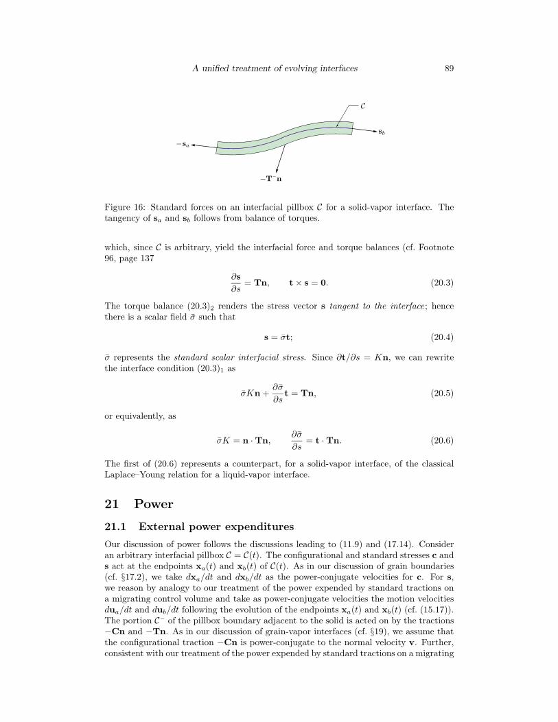
A unified treatment of evolving interfaces 89
− a
bs
s
−T−n
C
Figure 16: Standard forces on an interfacial pillbox C for a solid-vapor interface. Thetangency of sa and sb follows from balance of torques.
which, since C is arbitrary, yield the interfacial force and torque balances (cf. Footnote96, page 137
∂s∂s
= Tn, t × s = 0. (20.3)
The torque balance (20.3)2 renders the stress vector s tangent to the interface; hencethere is a scalar field σ such that
s = σt; (20.4)
σ represents the standard scalar interfacial stress. Since ∂t/∂s = Kn, we can rewritethe interface condition (20.3)1 as
σKn +∂σ
∂st = Tn, (20.5)
or equivalently, as
σK = n · Tn,∂σ
∂s= t · Tn. (20.6)
The first of (20.6) represents a counterpart, for a solid-vapor interface, of the classicalLaplace–Young relation for a liquid-vapor interface.
21 Power
21.1 External power expenditures
Our discussion of power follows the discussions leading to (11.9) and (17.14). Consideran arbitrary interfacial pillbox C = C(t). The configurational and standard stresses c ands act at the endpoints xa(t) and xb(t) of C(t). As in our discussion of grain boundaries(cf. §17.2), we take dxa/dt and dxb/dt as the power-conjugate velocities for c. For s,we reason by analogy to our treatment of the power expended by standard tractions ona migrating control volume and take as power-conjugate velocities the motion velocitiesdua/dt and dub/dt following the evolution of the endpoints xa(t) and xb(t) (cf. (15.17)).The portion C− of the pillbox boundary adjacent to the solid is acted on by the tractions−Cn and −Tn. As in our discussion of grain-vapor interfaces (cf. §19), we assume thatthe configurational traction −Cn is power-conjugate to the normal velocity v. Further,consistent with our treatment of the power expended by standard tractions on a migrating

90 E. Fried & M. E. Gurtin
control volume, we use as a power-conjugate velocity for −Tn the motion velocity !ufollowing S(t) (cf. 11.8). Finally, the configurational force g, being internal, expends noexternal power. The (net) external power expended on C(t) therefore has the form (cf.(19.5))
[
c · dxdt
+ s · dudt
]b
a
−∫
C
(
Cn · v + Tn · !u)
ds. (21.1)
21.2 Internal power expenditures. Power balance
First of all, using the identity ∂V/∂s =!ϑ and the normal configurational force balance
(20.1), it follows that (cf. (17.13) and (17.15))[
c · dxdt
]b
a
=[
σW + τV]b
a=[
σW]b
a+∫
C
[
τ!ϑ− (σK + g − n · Cn)V
]
ds; (21.2)
thus, since v = V n,[
c · dxdt
]b
a
−∫
C
Cn · v ds =[
σW]b
a+∫
C
[
τ!ϑ− (σK + g)V
]
ds. (21.3)
Further, since s = σt and ε = t · e (cf. 15.13)), we may use (15.17) to obtain[
s · dudt
]b
a
=[
s · !u + σεW]b
a. (21.4)
Thus, since ∂ !u/∂s = !e − KV e (cf. (15.12))[
s · dudt
]b
a
=[
σεW]b
a+∫
C
(∂s∂s
· !u + s · (!e − KV e))
ds. (21.5)
On the other hand, since s = σt and t · !e = !ε− γ
!ϑ (cf. (15.15)),
s · !e = σ(!ε− γ
!ϑ); (21.6)
therefore[
s · dudt
]b
a
=[
σεW]b
a+∫
C
(∂s∂s
· !u + σ(!ε− γ
!ϑ) − σεKV
)
ds (21.7)
and, using the standard force balance (20.3)1,[
s · dudt
]b
a
−∫
C
Tn · !u ds =[
σεW]b
a+∫
C
[
σ(!ε− γ
!ϑ) − σεKV
]
ds. (21.8)
Combining (29.9) and (21.8) then yields the power balance
[
c · dxdt
+ s · dudt
]b
a
−∫
C
(
Cn · v + Tn · !u)
ds
=[
(σ + σε)W]b
a+∫
C
[
σ!ε+ τ
!ϑ−(
(σ + σε)K + g)
V]
ds, (21.9)

A unified treatment of evolving interfaces 91
where we have introduced the reduced configurational shear
τ = τ − σγ. (21.10)
The contributions to the internal power-expenditure, which should be compared withthose (cf. §17.2) for a grain boundary, therefore have the form:
• The term[
(σ+ σε)W]b
a(rather than
[
σW]b
a) represents power expended internally
as material is added to C at its endpoints.
• The term σ!ε represents an expenditure of power associated with interfacial stretch-
ing.
• The term τ!ϑ (rather than τ
!ϑ) represents an expenditure of power associated with
changes in the orientation of the interface.68
• The term −(σ+ σε)KV (rather than −σKV ) represents the expenditure of powerassociated with changes in interfacial length due to the curvature of the interface.
The expenditure −gV is as discussed following (17.16).
22 Atomic transport
22.1 Atomic balance
As in our treatment of bulk atomic transport, we consider N species of atoms, labelledα = 1, 2, . . . , N . In addition to atomic densities ρα and fluxes α distributed over thesolid, we account for interfacial atomic densities δα, (scalar) interfacial atomic fluxeshα, and a prescribed supply rα of atoms from the vapor to the solid surface. As before,we write ρα = ρα− and α = α− for the appropriate interfacial limits.
Let C = C(t) be an arbitrary interfacial pillbox. Then surface diffusion in the portionof S exterior to C results in fluxes hα
a and −hαb of α-atoms across xa and xb, bulk diffusion
results in a flow α · n of α-atoms from the solid into C across C−, and there is a flow rα
of α-atoms into C across C+ from the vapor (Figure 17). Hence, the net rate at whichatoms are added to C by diffusive transport and through the vapor supply is
−hα∣∣b
a+∫
C
(α · n + rα) ds. (22.1)
Accretion of the portion of the interface exterior to C results in fluxes −δαa Wa and
δαb Wb of α-atoms across xa and xb,69 while accretion of C results in a flow −ραV of
68One might, at first sight, be surprised at the term σγ in the power expenditure τϑ! = (τ − σγ)ϑ!.The presence of this term is a consequence of the fact that the interfacial stress s is tangent to theinterface, but the interfacial strain-rate e! is not; because of this dichotomy the standard interfacialstress power is given by (21.6). In the finite-strain theory the interfacial stress s is tangent to thedeformed interface; i.e., s = σt with t the unit tangent to the deformed interface. If in that theorywe let u denote the displacement relative to the reference configuration and consider ∇ and ∂/∂s as“material” operators and (. . . )! as the time-derivative following the interface as described materially,then, defining e = ∂u/∂s, it follows, as before, that e! = (ε! − γϑ!)t + (γ! + εϑ!)n. Thus in thefinite-strain theory the interfacial stress power has the form s ·e! = σ(ε! −γϑ!)(t · t)+(γt ·+εϑ!)(t ·n)and hence reduces to that used in the “small-deformation theory” in the small-strain limit, where t → tand n → n. This lends further credence to the form of the power expenditures described here.
69I.e., e.g., δαa (t)Wa(t) = δα(xa(t), t)Wa(t).

92 E. Fried & M. E. Gurtin
rα
α · n − ραV
hαa − δα
a Wa
− hαb + δα
b Wb
C
Figure 17: Transport of α-atoms into an interfacial pillbox C.
α-atoms into C across C− (Figure 17). Hence, the net rate at which atoms are added toC by accretive transport is
[
δαW]b
a−∫
C
ραV ds. (22.2)
In view of (22.1) and (22.2), the atomic balance for C takes the form
d
dt
∫
C(t)
δα ds = −[
hα − δαW]b
a+∫
C(t)
(α · n − ραV + rα)ds, (22.3)
for each species α, and by virtue of the integral transport theorem (14.29), we have thelocal balance70
!δα + (ρα − δαK)V = −∂hα
∂s+ α · n + rα (22.4)
on the interface for each species α.
22.2 Net atomic balance
Defining the net bulk and adatom densities and the atomic volume Ω through
ρ =N∑
β=1
ρβ , δ =N∑
β=1
δβ , Ω =1ρ, (22.5)
and the net fluxes and supply through
=N∑
β=1
β , h =N∑
β=1
hβ , r =N∑
β=1
rβ , (22.6)
we see that (22.4), when summed over all atomic species, yields the net atomic balance
!δ + (ρ− δK)V = −∂h
∂s+ · n + r. (22.7)
70Comparison of the interfacial atomic balance (22.4) with its bulk counterpart (3.2) reveals severalformal similarities and differences. The adatom densities and fluxes enter (22.4) in a manner completelyanalogous to that in which the bulk atomic densities and fluxes enter (3.2). Aside from the curvatureterm and the term accounting for the supply of atoms from the vapor, what most distinguishes (22.4)from (3.2) is the presence of interaction terms that account for the accretion and the flow of atomsbetween the interface and the bulk.

A unified treatment of evolving interfaces 93
If adatom densities are neglected, then this net balance reduces to an equation for thenormal velocity:
V = Ω(
− ∂h
∂s+ · n + r
)
. (22.8)
For a substitutional alloy the lattice constraint (5.1) and the substitutional flux con-straint (5.4) imply that ρ = ρsites and = 0; hence the net atomic balance (22.7) takesthe form
!δ − δKV + ρsitesV = −∂h
∂s+ r (22.9)
whose sole coupling with the remaining field equations is through the kinematical termsV and K and, possibly, through the net flux h via additional constitutive information.If adatom densities are neglected, then (22.9) reduces to
V = Ω(
− ∂h
∂s+ r
)
, (22.10)
withΩ =
1ρsites
constant. Thus, when both adatom densities and surface diffusion are neglected, theevolution of an interface between a substitutional alloy and a vapor is governed solely bythe atomic supply r.
23 Free-energy imbalance
23.1 Energy flows due to atomic transport. Global imbalance
We assume that, if the material is unconstrained, then, for each species α, the chemicalpotential µα of the solid at its surface is the limiting value µα− of the bulk chemicalpotential. For a substitutional alloy, the individual chemical potentials are not welldefined in bulk; the relative chemical potentials must be used. We assume that, for anytwo species α and β, the limiting value µαβ− of the relative chemical potential is equalto the difference µα − µβ of chemical potentials of the solid at its surface. Thus we havethe chemical interface-conditions:
µα = µα−
µα − µβ = µαβ−
for an unconstrained material,for a substitutional alloy.
(23.1)
Motivated by the desire to describe processes such as molecular beam epitaxy, whereatoms are supplied directly at the film surface and the vapor cannot simply be modeledas a reservoir, we introduce for each species α an external supply rα of α-atoms, withconcomitant supply µαrα of energy. Therefore, in contrast to the discussion of moreclassical evaporation-condensation in §19, we do not find it necessary to endow the vaporwith a chemical potential.71 However, in §28 we will discuss a different class of vapor-interaction equations in which the vapor is considered as a reservoir for atoms endowed
71The discussion of evaporation-condensation (§19, for a single species) was based on the tacit assump-tion that there exist an infinitesimally thin transition-layer across which there is flow r of atoms from aquiescent reservoir at chemical potential µv to the solid at potential µ, a flow proportional to µv − µ.

94 E. Fried & M. E. Gurtin
with chemical potentials µαv , and for which rα is no longer arbitrarily prescribed, but is,
instead, a constitutive variable.The energy flow into a migrating pillbox C due to atomic transport includes contribu-
tions associated with diffusion, accretion, and the supply of atoms from the vapor. Thediffusion of α-atoms within the interface results in energy fluxes µα
ahαa and −µα
b hαb across
xa and xb; the diffusion of α-atoms in the solid results in an energy flow µαα · n acrossC−; the supply rα of α-atoms from the vapor results in an energy flow µαrα. The netrate at which energy is supplied to C by diffusion and evaporation-condensation is hencegiven by (cf. (19.13))
−N∑
α=1
[
µαhα]b
a+
N∑
α=1
∫
C
µα(α · n + rα) ds. (23.2)
The motion of the interface results in energy fluxes −µαa δ
αa Wa and µα
b δαb Wb associated
with the accretive transport of α-atoms across the endpoints xa and xb of C. In addi-tion, the motion of the interface results in an energy flow −µαρα−V associated with theaccretive transport of α-atoms from the solid across C−. Hence, the net rate at whichenergy is added to C by the accretive transport of atoms is
N∑
α=1
[
µαδαW]b
a−
N∑
α=1
∫
C
µαραV ds. (23.3)
Letting ψ denote the free energy of the interface and bearing in mind (21.1), (23.2),and (23.3), the free-energy imbalance for an arbitrary interfacial pillbox C = C(t) takesthe form
d
dt
∫
C
ψ ds
︸ ︷︷ ︸
free energy
≤[
c · dxdt
]b
a
−∫
C
Cn · v ds
︸ ︷︷ ︸
power expendedby configurational forces
+[
s · dudt
]b
a
−∫
C
Tn · !u ds
︸ ︷︷ ︸
power expendedby standard forces
+N∑
α=1
[
µα(−hα + δαW )]b
a+
N∑
α=1
∫
C
µα(α · n − ραV + rα) ds
︸ ︷︷ ︸
energy flow by atomic transport
. (23.4)
23.2 Dissipation inequality
In view of (21.9), (22.4), and the integral transport theorem (14.29), the free-energyimbalance (23.4) for C becomes
∫
C
(!ψ − ψKV ) ds +
(#)︷ ︸︸ ︷[(
ψ −N∑
α=1
µαδα − σε− σ
)
W
]b
a
≤∫
C
(
σ!ε+ τ
!ϑ−(
σ +N∑
α=1
µαδα + σε
)
KV − gV
)
ds
−N∑
α=1
[
µαhα]b
a+
N∑
α=1
∫
C
µα
(!δα +
∂hα
∂s
)
ds. (23.5)

A unified treatment of evolving interfaces 95
Since C is arbitrary, so also are the tangential velocities Wa and Wb of the endpoints ofC; thus, since the only term in (23.5) dependent on these velocities is the term (#), wehave the interfacial Eshelby relation72
σ = ψ −N∑
α=1
δαµα − σε, (23.6)
which is an analog of the bulk Eshelby relation (12.15).Since
N∑
α=1
[
µαhα]b
a=
N∑
α=1
∫
C
(
µα ∂hα
∂s+ hα ∂µα
∂s
)
ds, (23.7)
we may use (23.6) to rewrite (23.5) as∫
C
(!ψ − σ
!ε− τ
!ϑ−
N∑
α=1
(
µα!δα − hα ∂µα
∂s
)
+ gV
)
ds ≤ 0; (23.8)
since C is arbitrary, this yields the interfacial dissipation inequality
!ψ − σ
!ε− τ
!ϑ−
N∑
α=1
(
µα!δα − hα ∂µα
∂s
)
+ gV ≤ 0. (23.9)
When adatom densities are neglected, the “constraint” +δ = +0 renders (23.9) indepen-dent of the chemical potentials µα; in this case, as in classical theories of continua, thechemical potentials µα on S should be considered as indeterminate (not constitutivelydeterminate).
72In the absence of standard interfacial stress, the configurational stress within the interface has theform c = σt + τn, wit σ = ψ −
∑Nα=1 δ
αµα. This result, which, like the relation σ = ψ arising in ourdiscussion of grain boundaries (cf. (17.21)), has a purely energetic structure. In this case it is legitimateto view σ as an interfacial tension. But when standard stress is taken into account this interpretation isno longer valid. To explain this, consider the three-dimensional theory. There the interface is a surfaceS and the interfacial stresses are tensorial. The standard stress T is a symmetric, tangential tensor fieldon S: in terms of Cartesian coordinates with subscripts 1 and 2 associated with the tangent plane at apoint x on S, the component matrix of T(x) has the form
T11 T12 0T12 T22 00 0 0
(cf., e.g., Gurtin and Murdoch (1975) and the review of Shchukin and Bimberg (1999)). On the otherhand, the configurational surface stress is a tensor field with both normal and tangential parts; thetangential part, which is the part relevant to a discussion of surface tension and which might be comparedto the vector field c of the two-dimensional theory, has the form
Ctan =
(
ψ −N∑
α=1
δαµα)
P − (∇Su)!T,
where ∇S is the surface gradient on S, and P, the projector onto S, has component matrix at x of theform
1 0 00 1 00 0 0
.
Only in the absence of standard surface stress does Ctan take the form Ctan =(
ψ −∑N
α=1 δαµα)
P of apure tension; otherwise, Ctan is a generic tangential tensor field. One could, of course, think of ψ−δαµα
as a surface tension, and this is often done (cf. Shchukin and Bimberg, 1999), but what is more cogentis the form of Ctan, which should be compared with the form C =
(
Ψ−∑N
α=1 ραµα)
1− (∇u)!T of thebulk Eshelby tensor established in §12, a comparison that identifies Ctan as an Eshelby tensor for thesurface S (cf. Gurtin, 1995, 2000).

96 E. Fried & M. E. Gurtin
24 Normal configurational force balance revisited
24.1 Mechanical potential FSince we account for deformation and atomic transport, the bulk configurational stressC is determined by the Eshelby relation (12.15):
C =(
Ψ−N∑
α=1
ραµα
)
1 − (∇u)!T.
Thus, in view of the interfacial Eshelby relation (23.6), we may write the normal config-urational force balance (20.1) in a form,
N∑
α=1
(ρα − δαK)µα = Ψ− Tn · (∇u)n − (ψ − σε)K − ∂τ
∂s− g, (24.1)
which equates terms representing transport to those that are purely mechanical. Thus,for
F def= Ψ− Tn · (∇u)n − (ψ − σε)K − ∂τ
∂s− g, (24.2)
we may rewrite the normal configurational force balance in the formN∑
α=1
(ρα − δαK)µα = F ; (24.3)
we refer to F as the mechanical potential.When g = 0, F represents the variational derivative of the total free energy with
respect to variations of the position of the interface, holding the composition fixed. Thisfield appears first in the works of Wu (1996), Freund (1998), and Norris (1998), who,working within a framework that does not explicitly account for atomic species, followHerring (1951) (cf. our discussion of (1.1)) in viewing the surface gradient of this potentialas the driving force for surface diffusion.73 That (24.3) is compatible with this point ofview follows upon neglecting adatom densities and restricting attention to a single species.A useful alternative form for F follows upon noting that, since τ = σγ + τ (cf. (21.10))and ∂σ/∂s = t · Tn = n · Tt (cf. (20.6)),
∂τ
∂s=
∂σ
∂sγ + σ
∂γ
∂s+
∂τ
∂s= γn · Tt + σ
∂γ
∂s+
∂τ
∂s; (24.4)
hence
F = Ψ− Tn · (∇u)n − γn · Tt − (ψ − σε)K − σ∂γ
∂s− ∂τ
∂s− g. (24.5)
Another form for F and one that we find interesting, but do not use, is
F = Φ + ε trT − ψK − σ∂γ
∂s− ∂τ
∂s− g, (24.6)
with Φ the free enthalpy (cf. (7.15)). The verification of (24.6) involves the relations1 = t ⊗ t + n ⊗ n, e = (∇u)t = εt + γn, and σK = n · Tn.
73Related studies are those of Asaro and Tiller (1972), Rice and Chuang (1981), and Spencer, Voorhees,and Davis (1991), who restrict attention to a surface free-energy that is constant. See, also, Freundand Jonsdottir (1993), Grilhe (1993), Gao (1994), Freund (1995), Spencer and Meiron (1994), Yangand Srolovitz (1994), Suo and Wang (1997), Wang and Suo (1997), Xia, Bower, Suo and Shih (1997),Leonard and Desai (1998), Gao and Nix (1999), Shchukin and Bimberg (1999), Danescu (2001), Spencer,Voorhees, and Tersoff (2001), Xiang and E (2002).

A unified treatment of evolving interfaces 97
24.2 Substitutional alloys. Interfacial chemical potentials µα interms of the relative chemical-potentials µαβ
For a substitutional alloy the bulk densities ρα are subject to the lattice constraint (5.1).As a consequence of this constraint, the individual chemical potentials µα in bulk awayfrom the interface are not well-defined; only the relative chemical potentials µαβ havemeaning. At the interface the limiting values of these relative potentials are relatedto the chemical potentials of the solid at the interface through the chemical interface-conditions (23.1), µα − µβ = µαβ−. Thus, limiting our discussion to the interface andwriting µαβ = µαβ−, we have the interface condition
µα − µβ = µαβ . (24.7)
On the other hand,
there is no lattice constraint for the diffusion of adatoms
and, as is clear from (24.1), it is the individual chemical potentals µα that enter the basicequations on S. In accord with this, we now show that the individual chemical potentialson S are uniquely determined — by what is essentially the normal configurational forcebalance — when the relative chemical potentials are known in the film.
If we define effective densities
ραef = ρα − δαK, (24.8)
then (24.3) becomes
ραef µ
α = F . (24.9)
It is convenient to define an effective net density ρef, effective concentrations cαef, and an
effective net atomic volume Ωef through
ρef =N∑
α=1
ραef, cα
ef =ραef
ρef, Ωef =
1ρef
. (24.10)
Then, choosing an atomic species α arbitrarily, we may use an argument of Larche andCahn74 to express µα in terms of the N −1 relative chemical-potentials µαβ and the sumρβefµ
βα. Since µβ = µα − µαβ ,
N∑
β=1
ρβefµ
β =N∑
β=1
ρβef(µ
α − µαβ) = ρefµα −
N∑
β=1
ρβefµ
αβ ,
and the normal configurational force balance (24.9) yields an identity,
µα =N∑
β=1
cβefµ
αβ + ΩefF
=N∑
β=1
cβefµ
αβ + Ωef
Ψ− Tn · (∇u)n − (ψ − σε)K − ∂τ
∂s− g
, (24.11)
which, for a substitutional alloy, gives the individual chemical potential µα of each speciesα in terms of the chemical-potentials µαζ of α relative to all other species ζ. We refer to(24.11) as the configurational-chemistry relations.
Conversely, if (24.11) holds for all α, then µαβ = µα −µβ and (24.9) is satisfied. Thuswe have the following result:
74Larche and Cahn (1985, Appendix 1).

98 E. Fried & M. E. Gurtin
Equivalency Theorem for Substitutional Alloys The configurational-chemistry relations,
µα =N∑
β=1
cβefµ
αβ + ΩefF , α = 1, 2, . . . , N, (24.12)
are satisfied if and only if both the normal configurational force balance,N∑
α=1
(ρα − δαK)µα = F ,
and the relative chemical-potential relations,
µαβ = µα − µβ , α,β = 1, 2, . . . , N,
are satisfied.
Thus, when discussing substitutional alloys we may equally well use the normal configura-tional force balance or the onfigurational-chemistry relations, provided that in the formercase we account also for the relative chemical-potential relations. This result is centralto what follows.
25 Constitutive equations for the interface
Since there is no lattice constraint for the diffusion of adatoms along the interface, thediscussion of this section is valid whether or not the associated bulk material is subjectto a lattice constraint.
25.1 General relations
Our discussion of constitutive equations is guided by the interfacial dissipation inequality(23.9), viz.,
!ψ − σ
!ε− τ
!ϑ−
N∑
α=1
(
µα!δα − hα ∂µα
∂s
)
+ gV ≤ 0,
and follows the format set out in §17.8.Let
+δ = (δ1, δ2, . . . , δN ), +µ = (µ1, µ2, . . . , µN ).
Granted essentially linear dissipative response, we consider constitutive equations giv-ing75
ψ, σ, τ , +µ as functions of (ε,ϑ,+δ )
in conjunction with constititutive equations for hα and g of the specific form
hα = −N∑
β=1
Lαβ ∂µβ
∂s− 6αV,
g = −N∑
α=1
Bα ∂µα
∂s− bV,
(25.1)
75Since ε = t · (∇u)t is invariant for transformations of the form ∇u &→ ∇u+W, with W an arbitraryskew-symmetric tensor, the constitutive equations considered here have the requisite invariance underinfinitesimal changes of observer.
A unified treatment of evolving interfaces 99
with coefficients possibly dependent on (ε,ϑ,+δ ).76
Then, appealing to the discussion of §17.8, we find that the free energy determines thestandard scalar interfacial stress, the reduced shear, and the chemical potentials throughthe relations
σ =∂ψ(ε,ϑ,+δ )
∂ε,
τ =∂ψ(ε,ϑ,+δ )
∂ϑ,
µα =∂ψ(ε,ϑ,+δ )
∂δα,
(25.2)
and that the coefficient matrix of the equations (25.1) must be positive semi-definite.In view of (21.10), τ = σγ + τ and (25.2)1,2 yield an auxiliary constitutive relation
showing that the configurational shear τ depends also on the interfacial shear-strain γ.An increased understanding of τ is achieved by introducing
ψ(e,ϑ,+δ ) = ψ(e · t,ϑ, +ρ ) = ψ(ε,ϑ, +ρ ). (25.3)
Specifially, differentiating with respect to ϑ, we obtain
∂ψ(e,ϑ,+δ )∂ϑ
=∂ψ(ε,ϑ, +ρ )
∂ε
∂(e · t)∂ϑ
+∂ψ(ε,ϑ, +ρ )
∂ϑ, (25.4)
which, by (25.2)1,2, (14.1), the definition (15.10)2 of γ, and the relation τ = σγ+ τ gives
∂ψ(e,ϑ, +ρ )∂ϑ
= τ. (25.5)
Thus, whereas τ accounts for configurational shear arising solely from changes of interfa-cial orientation, τ accounts also for configurational shear generated by tensile stretchingof the interface.
Within the context of small deformations, it is reasonable to restrict attention to freeenergies that are quadratic in the tensile strain ε and, thus, have the form
ψ(ε,ϑ,+δ ) = ψ0(ϑ,+δ ) + w(ε,ϑ,+δ ), (25.6)
with strain energy w of the form
w(ε,ϑ,+δ ) = σ0(ϑ,+δ )ε+ 12k(ϑ,+δ )ε2. (25.7)
Here, ψ0(ϑ,+δ ) is the strain-free surface energy, σ0(ϑ,+δ ) is the residual surface stress,and k(ϑ,+δ ) is the surface elasticity. Because atoms on the free surface are not bondedto the maximum number of nearest neighboring atoms, a residual surface stress is to beexpected (Shchukin and Bimberg, 1999).
The expressions for σ, τ , and µα determined by (25.2) under this specialization arestraightforward. However, the final field equations are cumbersome. For this reason, wework with the generic expression ψ = ψ(ε,ϑ,+δ ).
76The experiments of Barvosa-Carter and Aziz (2001) and first-principles calculations of Van de Walle,Asta, and Voorhees (2002) suggest that strain dependence of the mobilities may be important.

100 E. Fried & M. E. Gurtin
25.2 Uncoupled relations for hα and g
A simplified form of (25.1) would take the classical Fickean form
hα = −N∑
β=1
Lαβ ∂µβ
∂s(25.8)
in conjunction with the simple kinetic relation
g = −bV (25.9)
that formed the basis of our discussion of grain boundaries. Here the coefficients Lαβ ,which represent the mobility of the atoms on the interface, are presumed to form apositive semi-definite matrix, while b ≥ 0. The dissipation then has the form
D =N∑
α,β=1
Lαβ(ε,ϑ,+δ )∂µα
∂s
∂µβ
∂s︸ ︷︷ ︸
dissipation induced by surface diffusion
+ b(ε,ϑ,+δ )V 2
︸ ︷︷ ︸
dissipation accompany-ing the attachment
of vapor atoms
. (25.10)
We henceforth work with the uncoupled relations (25.8) and (25.9). This choice ismade for convenience only; the generalization of the resulting equations to situationsinvolving the more general coupled relations (25.1) is straightforward. An argument insupport of the uncoupled relations is that (25.8) represents the flow of atoms withinthe interface, while (25.9) represents an interaction of the solid surface with the vaporenvironment. But we do believe that there might be situations in which there is couplingbetween the diffusive adatom-flow described by +h and the solid-vapor interaction asdescribed by g. Such coupling might be especially important when studying film growth,since the kinetics of the deposition process and the small length scales involved renderthis process of a nature far different than the processes leading, for example, to relationsthat describe classical surface diffusion.
26 Governing equations at the interface
26.1 Equations with adatom densities included
While generally considered negligible, adatom densities would seem important in describ-ing the segregation of atomic species at a solid-vapor interface.77 Moreover, the parabolicnature of the atomic balances when adatom densities are included might serve to reg-ularize the overall system of partial differential equations, which is typically unstable.Regardless of whether adatom densities are included or neglected, our theory accountsfor the presence of adatoms and their diffusion via the interfacial atomic balances.
(a) General relations
The basic interfacial balances are the standard force-balance, the atomic balance, andthe normal configurational force balance; for the case of a substitutional alloy, the con-figurational balance with the relations for the relative chemical potentials together are
77Spencer, Voorhees, and Tersoff (2001) assert that: “surface segregation can make the surface com-position differ from the bulk and the overall surface density of components could be nonuniform.” Seealso Lu and Suo (2001, 2002), who use a Cahn–Hilliard type theory to study segregation of a planartwo-phase monolayer on a strained substrate.

A unified treatment of evolving interfaces 101
equivalent to the configurational-chemistry relations together with the relations for therelative chemical potentials. The standard force and atomic balances are (cf. §20.2, §22)
Tn = σKn +∂σ
∂st,
!δα + (ρα − δαK)V = −∂hα
∂s+ α · n + rα,
(26.1)
while the normal configurational force balance and the configurational-chemistry relationsfor substitutional alloys take the respective forms
N∑
α=1
(ρα − δαK)µα = F , µα =N∑
β=1
cβefµ
αβ + ΩefF (26.2)
(cf. (24.3), (24.5), (24.12)), with
F = Ψ− Tn · (∇u)n − γn · Tt − (ψ − σε)K − σ∂γ
∂s− ∂τ
∂s− g. (26.3)
As asserted in the equivalency theorem for substitutional alloys (page 98), for such mate-rials imposing (26.2)2 ensures satisfaction of both (26.2)1 and the relations µαβ = µα−µβ .
The balances are coupled to the constitutive relations
σ =∂ψ(ε,ϑ,+δ )
∂ε, τ =
∂ψ(ε,ϑ,+δ )∂ϑ
, µα =∂ψ(ε,ϑ,+δ )
∂δα(26.4)
(cf. §25.2) and
hα = −N∑
β=1
Lαβ ∂µβ
∂s, g = −bV. (26.5)
In (26.5) the constitutive moduli Lαβ and g are possibly dependent on (ε,ϑ,+δ ).By (26.4), writing
ψ(ε,ϑ,+δ ) = ψ(ε,ϑ,+δ )
and omitting the arguments (ε,ϑ,+δ ), we find that
(ψ − σε)K + σ∂γ
∂s+
∂τ
∂s
=(
ψ +∂2ψ
∂ϑ2− ε
∂ψ
∂ε
)
K +∂2ψ
∂ε∂ϑ
∂ε
∂s+∂ψ
∂ε
∂γ
∂s+
N∑
β=1
∂2ψ
∂δβ∂ϑ
∂δβ
∂s, (26.6)
Thus, combining the interfacial balances and the constitutive relations, we arrive at thestandard force and atomic balances
Tn =∂ψ
∂εKn +
(∂2ψ
∂ε2∂ε
∂s+
∂2ψ
∂ε∂ϑK +
N∑
β=1
∂2ψ
∂ε∂δβ
∂δβ
∂s
)
t,
!δα + (ρα − δαK)V =
∂
∂s
( N∑
β=1
Lαβ ∂µβ
∂s
)
+ α · n + rα,
(26.7)

102 E. Fried & M. E. Gurtin
and find that the mechanical potential F used in describing the normal configurationalforce balance and configurational-chemistry relations (26.2) has the form
F = Ψ− Tn · (∇u)n − γn · Tt
−(
ψ +∂2ψ
∂ϑ2− ε
∂ψ
∂ε
)
K − ∂2ψ
∂ε∂ϑ
∂ε
∂s− ∂ψ
∂ε
∂γ
∂s−
N∑
β=1
∂2ψ
∂δβ∂ϑ
∂δβ
∂s+ bV. (26.8)
Consider the atomic balance (26.7)2. If we define moduli
καβad =
∂2ψ
∂δα∂δβ, Dαβ
ad =N∑
γ=1
Lαγκγβad , (26.9)
with Dαβad the surface diffusivity of α relative to β, then the interfacial-diffusion term in
(26.7) has the form
∂
∂s
( N∑
β=1
Lαβ ∂µβ
∂s
)
=∂
∂s
N∑
β=1
Dαβad
∂δβ
∂s+
N∑
β=1
Lαβ
(∂2ψ
∂δβ∂ε
∂ε
∂s+
∂2ψ
∂δβ∂ϑ
∂ϑ
∂s
)
.
(26.10)
Thus, bearing in mind the term (δα)! in (26.7)2, we note that if the matrix with entriesDαβ
ad is positive definite, then (26.7)2, as a system of partial differential equations for theadatoms δα (considering the remaining fields as fixed), is parabolic and as such shouldhave a regularizing effect on the evolution of the interface.
(b) Chemical potentials at the surface. Chemical compatibility
For an unconstrained material, the chemical potentials µα of the surface, needed in thenormal configurational force balance (26.2)1, may be determined directly through thelimit relation
µα = µα−. (26.11)
On the other hand, these chemical potentials are given by the relations µα = ∂ψ/∂δα
and by the limit relations (26.11) supplemented by the bulk constitutive relations (7.17):
µα =∂ψ(ε,ϑ,+δ )
∂δα=∂Φ(T, +ρ )∂ρα
. (26.12)
Similarly, for a substitutional alloy, the relative chemical potentials µαβ on the solidsurface may be determined through the limit relation
µαβ = µαβ−, (26.13)
and, in addition, (9.36) yields
µαβ =∂ψ(ε,ϑ,+δ )
∂δα− ∂ψ(ε,ϑ,+δ )
∂δβ=∂Φ(β)(T, +ρ )
∂ρα; (26.14)
Granted a knowledge of these relative chemical potentials, the surface values of thechemical potentials µα are given by the configurational-chemistry relations (26.2)2, aprocedure that ensures satisfaction of the normal configurational force balance.

A unified treatment of evolving interfaces 103
Equations (26.12) and (26.14) might be termed chemical-compatibility relations asthey represent compatibility between the composition of the interface and that of thebulk material. When
(∂ψ(ε,ϑ,+δ )
∂δ1,∂ψ(ε,ϑ,+δ )
∂δ2, . . . ,
∂ψ(ε,ϑ,+δ )∂δN
)
is an invertible function of +δ, (26.12) furnishes explicit relations giving the adatom den-sities as functions of the bulk densities (as well as ε, ϑ, and T).78 A similar assertioncannot be made for (26.14). Note that, for mechanically simple materials, (26.12) and(26.14) have the respective forms (cf. (7.34), (9.63), (9.64))
µα =∂ψ(ε,ϑ,+δ )
∂δα= µα
0 (+ρ ) − Nα · T (26.15)
and
µαβ =∂ψ(ε,ϑ,+δ )
∂δα− ∂ψ(ε,ϑ,+δ )
∂δβ= µα
0 (+ρ ) − µβ0 (+ρ ) − Nαβ · T. (26.16)
(c) Equations neglecting standard surface stress (s ≡ 0)
In this case ψ = ψ(ϑ,+δ ) and the standard force-balance (26.7)1 has the simple form
Tn = 0, (26.17)
asserting that the solid-vapor interface be (standard) traction-free, and the atomic bal-ance (26.7)2 becomes
!δα + (ρα − δαK)V =
∂
∂s
( N∑
β=1
Lαβ ∂µβ
∂s
)
+ α · n + rα. (26.18)
Further, the normal configurational force balance (26.8) for unconstrained materials andthe configurational-chemistry relations for substitutional alloys have the respective forms
N∑
α=1
(ρα − δαK)µα = Ψ−(
ψ +∂2ψ
∂ϑ2
)
K −N∑
β=1
∂2ψ
∂δβ∂ϑ
∂δβ
∂s+ bV (26.19)
and
µα =N∑
β=1
cβefµ
αβ + Ωef
Ψ−(
ψ +∂2ψ
∂ϑ2
)
K −N∑
β=1
∂2ψ
∂δβ∂ϑ
∂δβ
∂s+ bV
. (26.20)
We now specialize the normal configurational force balance and the configurational-chemistry relations to mechanically simple materials. For such materials the relation(7.31) for the free energy and the Gibbs relation (8.3) yield
Ψ = 12 T · K[T] +
N∑
α=1
ραµα0 (+ρ ); (26.21)
78Spencer, Voorhees and Tersoff (2001) do not consider a dependence of interfacial free-energy onadatom densities, but instead posit constitutive relations of the form δα = λρα, with λ constant. Fora nondeformable, unconstrained material, relations of this form would follow from (26.12), grantedinterfacial and bulk free-energies of the form ψ = 1
2Λ∑N
α=1(δα)2 and Ψ = 12λΛ
∑Nα=1(ρα)2, with Λ
constant.

104 E. Fried & M. E. Gurtin
hence the normal configurational force balance (26.19) for an unconstrained, mechanicallysimple material takes the form
N∑
β=1
(ρα − δαK)µα =N∑
α=1
ραµα0 + 1
2T · K[T]
−(
ψ +∂2ψ
∂ϑ2
)
K −N∑
β=1
∂2ψ
∂δβ∂ϑ
∂δβ
∂s+ bV. (26.22)
The analogous result for a substitutional alloy is not as simple to derive. To beginwith, we assume there are no vacancies; the relations (9.65)1,3 and (9.58) for the freeenergy and chemical potentials and the free-energy conditions at zero-stress, (9.45), thenimply that
Ψ = 12T · K[T] +
N∑
α=1
ραµα0 (+ρ ),
µαβ = µα0 (+ρ ) − µβ
0 (+ρ ) − Nαβ · T.
(26.23)
Thus, writing
R = −(
ψ +∂2ψ
∂ϑ2
)
K −N∑
β=1
∂2ψ
∂δβ∂ϑ
∂δβ
∂s+ bV,
we may use (24.8), (24.10), and (26.20) to show that
ρef µα =
N∑
β=1
ρβef µ
αβ + Ψ + R
= ρef µα0 −
N∑
β=1
ρβef µ
β0 −
N∑
β=1
ρβef N
αβ · T + 12T · K[T] +
N∑
β=1
ρβµβ0 + R
= ρef µα0 +
N∑
β=1
δβµβ0K −
N∑
β=1
ρβef N
αβ · T + 12T · K[T] + R.
The configurational-chemistry relations (26.20) for a mechanically simple, substitutionalalloy without vacancies therefore takes the form
µα − µα0 =
N∑
β=1
cβef N
βα · T + 12T · K[T]
−(
ψ +∂2ψ
∂ϑ2−
N∑
β=1
δβµβ0
)
K −N∑
β=1
∂2ψ
∂δβ∂ϑ
∂δβ
∂s+ bV. (26.24)
26.2 Equations when adatom densities are neglected
(a) Balances
The basic interfacial balances are (26.1) and (26.2) with the terms involving adatomsdeleted. The balances for standard forces and atoms therefore take the form
Tn = σKn +∂σ
∂st,
ραV = −∂hα
∂s+ α · n + rα,
(26.25)

A unified treatment of evolving interfaces 105
while the normal configurational force balance and the configurational-chemistry relations(for substitutional alloys) take the respective forms
N∑
α=1
ραµα = F , µα =N∑
β=1
cβµαβ + ΩF , (26.26)
with mechanical potential F , as before, given by (26.3). In writing (26.26) we have usedthe fact that, for +δ ≡ 0, the defining relations for Ωef in (24.8) and cβ
ef in (24.10) take therespective forms
Ωef = Ω =1
ρsites, cβ
ef = cβ =ρβ
ρsites, (26.27)
with Ω the atomic volume and cβ the concentration of species β.
(b) Constitutive relations. Indeterminacy of the chemical potentials
The treatment of chemical potentials in the absence of an accounting of adatom densitiesis somewhat delicate: since µα(δα)! = 0 for each α, the interfacial dissipation inequality(23.9) reduces to
!ψ − σ
!ε− τ
!ϑ+
N∑
α=1
hα ∂µα
∂s+ gV ≤ 0; (26.28)
the absence of a field conjugate to the surface chemical potentials µα renders themindeterminate on S; that is, not viable as independent variables in the constitutiverelations for the interface. Thus, in view of the dissipation inequality (26.28), arguing asfor (26.4) and (26.5), we are led to the constitutive relations
σ =∂ψ(ε,ϑ)∂ε
, τ =∂ψ(ε,ϑ)∂ϑ
, (26.29)
and
hα = −N∑
β=1
Lαβ ∂µβ
∂s, g = −bV, (26.30)
with moduli Lαβ and g allowed to depend on (ε,ϑ).By (26.29), writing ψ(ε,ϑ) = ψ(ε,ϑ), we find that
(ψ − σε)K + σ∂γ
∂s+
∂τ
∂s=(
ψ +∂2ψ
∂ϑ2− ε
∂ψ
∂ε
)
K +∂2ψ
∂ε∂ϑ
∂ε
∂s+∂ψ
∂ε
∂γ
∂s. (26.31)
Thus, if we combine the interfacial balances and the constitutive relations, we arrive atthe standard force and atomic balances
Tn =∂ψ
∂εKn +
(∂2ψ
∂ε2∂ε
∂s+
∂2ψ
∂ε∂ϑK
)
t,
ραV =∂
∂s
( N∑
β=1
Lαβ ∂µβ
∂s
)
+ α · n + rα.
(26.32)

106 E. Fried & M. E. Gurtin
Further, the normal configurational force balance and the configurational-chemistry re-lations for substitutional alloys are given by (26.26) with mechanical potential
F = Ψ− Tn · (∇u)n − γn · Tt
−(
ψ +∂2ψ
∂ϑ2− ε
∂ψ
∂ε
)
K − ∂2ψ
∂ε∂ϑ
∂ε
∂s− ∂ψ
∂ε
∂γ
∂s+ bV, (26.33)
which is simply (26.8) with the term involving adatoms dropped.
(b) Equations based on a quadratic strain-energy
A theory that might be useful in accessing the effects of surface stress might be basedon a free energy of the form (cf. (26.4)1)
ψ = ψ0(ϑ) + w(ε,ϑ), (26.34)
with quadratic strain-energy
w(ε) = σ0(ϑ)ε+ 12k(ϑ)ε2. (26.35)
In this case, the scalar surface stress and reduced configurational shear are
σ = σ0(ϑ) + k(ϑ)ε, τ = ψ′0(ϑ) + σ′
0(ϑ)ε+ 12k′
0(ϑ)ε2. (26.36)
Further, by (15.10) and (15.11), the normal and tangential components (20.6)1 and(20.6)2 of the standard force balance reduce to
n · Tn =(
σ0(ϑ) + k(ϑ)t · ∂u∂s
)
K (26.37)
and
t · Tn =(
σ′0(ϑ) + k(ϑ)n · ∂u
∂s+ k′(ϑ)t · ∂u
∂s
)
K + k(ϑ)t · ∂2u∂s2
, (26.38)
while the mechanical potential becomes
F = Ψ− Tn · (∇u)n −
ψ0(ϑ) + ψ′′0 (ϑ) −
(
σ0(ϑ) − σ′′0 (ϑ))
t · ∂u∂s
+ 2σ′0(ϑ)n · ∂u
∂s
+ k(ϑ)(
n · ∂u∂s
)2
− 12
(
3k(ϑ) − k′′(ϑ))(
t · ∂u∂s
)2
+ 2k′(ϑ)(
t · ∂u∂s
)(
n · ∂u∂s
)
K
−(
σ0(ϑ)n+ σ′0(ϑ)t+ k(ϑ)
(
t · ∂u∂s
)
n+(
n · ∂u∂s
)
t
+ k′(ϑ)(
t · ∂u∂s
)
t)
· ∂2u∂s2
+ bV.
(26.39)
A simplifying assumption of potential value for assessing the importance of surfacestress might be to take the residual stress and elasticity for the surface to be constant.Then, (26.37) and (26.38) simplify slightly to
n · Tn =(
σ0 + kt · ∂u∂s
)
K (26.40)

A unified treatment of evolving interfaces 107
and
t · Tn =(
kn · ∂u∂s
)
K + kt · ∂2u∂s2
, (26.41)
while (26.42) reduces to
F = Ψ− Tn · (∇u)n −(
ψ0(ϑ) + ψ′′0 (ϑ) − 3
2k
(
t · ∂u∂s
)2
+ k
(
n · ∂u∂s
)2
− σ0t ·∂u∂s
)
K
−(
σ0n + k
(
t · ∂u∂s
)
n +(
n · ∂u∂s
)
t
· ∂u∂s
)
· ∂2u∂s2
+ bV. (26.42)
so that even within this drastically simplified theory the standard force balance, thenormal configurational force balance, and, for a substitutional alloy, the configurational-chemistry relations are quite complicated.
Alternatively, consistent with the view of Shchukin and Bimberg (1999), we mightallow the free energy to be anisotropic but ignore interfacial elasticity, so that
ψ = ψ0(ϑ) + σ0(ϑ)ε,
σ = σ0(ϑ),
τ = ψ′0(ϑ) + σ′
0(ϑ)ε.
(26.43)
Then, the appropriately simplified versions of (26.37) and (26.38) combine to yield
Tn = σ0(ϑ)Kn + σ′0(ϑ)Kt; (26.44)
thus, writing∂u∂n
= (∇u)n,
it follows that
Tn · (∇u)n = σ0(ϑ)Kn · ∂u∂n
+ σ′0(ϑ)Kt · ∂u
∂n(26.45)
and we may replace (26.42) by
F = Ψ−(
ψ0(ϑ)+ψ′′0 (ϑ)+
(
σ0(ϑ)+2σ′0(ϑ))
n · ∂u∂n
−(
σ0(ϑ)− σ′0(ϑ)− σ′′
0 (ϑ))
t · ∂u∂s
)
K
−(
σ0(ϑ)n + σ′0(ϑ)t
)
· ∂2u∂s2
+ bV. (26.46)
Finally, if σ0 = constant and k = 0, then (26.44) and (26.46) specializes to yield
Tn = σ0Kn, (26.47)
and
F = Ψ−
ψ0(ϑ) + ψ′′0 (ϑ) + σ0
(
n · ∂u∂n
− t · ∂u∂s
)
K − σ0n · ∂2u∂s2
+ bV. (26.48)
As discussed in §17.5, the local stability of the evolution equation (17.32) for a grainboundary is determined by the sign of the coefficient of the curvature — the interfacialstiffness. In (26.48), the coefficient of the curvature is the sum of the interfacial stiffnessand the term σ0(enn−ett), with enn = n·∂u/∂n and ett = t·∂u/∂t. Thus, notwithstand-ing the term σ0n · ∂2u/∂s2, it appears that a tensile normal strain (for which enn > 0)and a compressive tangential strain (for which −ett > 0) should be stabilizing.

108 E. Fried & M. E. Gurtin
(c) Equations neglecting standard surface stress
Here the interface remains traction-free and the atomic balance becomes
ραV =∂
∂s
( N∑
β=1
Lαβ ∂µβ
∂s
)
+ α · n + rα, (26.49)
the normal configurational force balance has the form
N∑
α=1
ραµα = Ψ−(
ψ +∂2ψ
∂ϑ2
)
K + bV, (26.50)
and, for a substitutional alloy, the configurational chemistry relations become
µα =N∑
β=1
cβµαβ + Ω
Ψ−(
ψ +∂2ψ
∂ϑ2
)
K + bV
. (26.51)
Finally, restricting attention to mechanically simple materials, we find that (26.50)and (26.51), respectively, reduce to
N∑
α=1
ρα(µα − µα0 ) = 1
2T · K[T] −(
ψ +∂2ψ
∂ϑ2
)
K + bV (26.52)
and
µα − µα0 =
N∑
β=1
cβ Nβα · T + Ω
12T · K[T] −
(
ψ +∂2ψ
∂ϑ2
)
K + bV
. (26.53)
Granted cubic symmetry, so that Nαβ = ηαβ1 (cf. 9.68)), and assuming that b ≡ 0,(26.53) reduces to the following result of Spencer, Voorhees and Tersoff (2001, eqts.(2.10), (2.11)):79
µα − µα0 =
N∑
β=1
cβ ηβα trT + Ω
12T · K[T] −
(
ψ +∂2ψ
∂ϑ2
)
K
.
26.3 Addendum: Importance of the kinetic term g = −bV
In each of the cases discussed in the last two subsections, the normal configurational forcebalance contains the kinetic term bV resulting from the constitutive equation g = −bV forg, a dissipative force associated with the attachment of vapor atoms to the solid surface.The dissipation associated with g,80 measured per unit length of the interfacial curve, isbV 2; without this term the attachment process is nondissipative.
Interface conditions that play the role of the normal configurational force balance aretypically derived using an assumption of local equilibrium or using a chemical potentialderived as a variational derivative of the total free-energy with respect to variations in theconfiguration of the interface; thus the possibility of having a dynamical interface condi-tion involving V are ruled out from the start by the use of such variational paradigms,which, by their very nature, cannot involve the normal velocity V .
79Note that our ηβα is Ω times their modulus ηβα.80Cf. (25.10) and the remark following (23.9).

A unified treatment of evolving interfaces 109
To assess the importance of the kinetic term, consider a single atomic species andneglect bulk diffusion, so that ≡ 0 and the atomic volume Ω = 1/ρ is constant. Assumefurther that the mobility L for surface diffusion and the kinetic modulus b are constant,so that the atomic balance (26.49) and the normal configurational force balance (26.50)take the form
V = ΩL∂2µ
∂s2+ r, µ = Ω
Ψ−(
ψ +∂2ψ
∂ϑ2
)
K + bV
. (26.54)
The fieldµeq = Ω
Ψ−(
ψ +∂2ψ
∂ϑ2
)
K
represents the equilibrium chemical potential (the chemical potential when V = 0); usingthis field we may write the normal configurational force balance in the form µ = µeq +ΩbV . This relation and the atomic balance (26.54)1 yield the evolution equation
V − λ2 ∂2V
∂s2= ΩL
∂2µeq
∂s2+ r (26.55)
with
λ = Ω√
bL (26.56)
a material length-scale; the kinetic term g = −bV is therefore important at length scales oforder λ and smaller.81 Thus, whether or not the kinetic term is important depends on themagnitude of the product bL; consequently, when the Fickean mobility L is sufficientlylarge, the term g = −bV may be important even when the modulus b is small.
27 Interfacial couples. Allowance for an energetic de-pendence on curvature
The notorious instability of strained solid-vapor interfaces results in a wide variety ofsurface patterns and morphologies, an example being the faceted islands (Figure 18) ob-served by Tersoff, Spencer, Rastelli and von Kanel (2003). Such instabilities are reflectedby the underlying evolution equations82 and by the resulting difficulty of performing re-liable simulations, which motivates the need for physically-based regularized theories.83Regularizations that account for an energetic dependence on curvature (DiCarlo, Gurtinand Podio-Guidugli, 1992) but neglect surface stress and adatom densities, are usedTersoff, Spencer, Rastelli and von Kanel (2003) to describe the initial stages of islandformation and by Seigel, Miksis and Voorhees (2003) to study the formation of wrin-klings on a void surface.84 To arrive at a theory that allows for an energetic dependence
81This conclusion arose from conservations with Peter Voorhees.82Asaro and Tiller (1972), Grinfeld (1986), and Srolovitz(1989) showed that a planar layer under stress
may be unstable. Subsequent studies of related instabilities include Freund and Jonsdottir (1993), Grilhe(1993), Gao (1994), Freund (1995), Spencer and Meiron (1994), Yang and Srolovitz (1994), Suo and Wang(1997), Wang and Suo (1997), Xia, Bower, Suo and Shih (1997), Leonard and Desai (1998), Gao andNix (1999), Shchukin and Bimberg (1999), Phan, Kaplan, Gray, Adalsteinsson, Sethian, Barvosa-Carter,and Aziz (2001), Danescu (2001), Spencer, Voorhees, and Tersoff (2001), and Xiang and E (2002).
83Our perspective here is identical to that in §18. As opposed to a pragmatical approach in whichsupplemental terms involving higher-order derivatives are added to stabilize an equation, we seek regu-larizations that reflect a consideration of relevant physical mechanisms.
84As discussed above, the inclusion of adatoms may provide at least a partial regularization as doingso can, with appropriate constitutive assumptions, lead to parabolic evolution equations for the adatomdensities. However, constraining the curvature of the interface via an energetic dependence on curvatureshould provide a more effective regularization.

110 E. Fried & M. E. Gurtin
Figure 18: (a) STM image (108 × 108 nm2) of a faceted island obtained by depositingSi0.6Ge0.4 on Si(001). (b) Cross-section of the region near the top of the island, from anaverage of 30 line scans taken from left to right close to the middle of the island. Scalein nm. (Images courtesy of Tersoff, Spencer, Rastelli and von Kanel.)
on curvature, one may follow the steps taken in our extension of the classical theory ofgrain boundaries to allow for the study of facets and wrinklings (cf. §18). Specifically,we may introduce an interfacial couple stress and an interfacial internal couple togetherwith an configurational torque balance. Taking into account the torques exerted by theconfigurational force system, the configurational torque balance for an interfacial pillboxC is (cf. (18.1))
[
M + (x − 0)×c]b
a+∫
C
m ds +∫
C
[
(x − 0)×(g − Cn)]
ds = 0. (27.1)
The foregoing considerations leave intact the basic balances considered in our previoustreatment of strained solid-vapor interfaces. Thus, using the configurational force balanceand proceeding as in the derivation of (18.3), we obtain the local statement
∂2M
∂s2+∂m
∂s− σK − g + n · Cn = 0 (27.2)
of configurational torque balance.In the presence of interfacial couples, the net power expended on an interfacial pillbox
C must account for the action of the couple stress M at the endpoints of C and this leads

A unified treatment of evolving interfaces 111
to a free-energy imbalance of the form
d
dt
∫
C
ψ ds ≤[
Mdϑ
dt
]b
a
+[
c · dxdt
]b
a
−∫
C
Cn · v ds +[
s · dudt
]b
a
−∫
C
Tn · !u ds
+N∑
α=1
[
µα(−hα + δαW )]b
a+
N∑
α=1
∫
C
µα(α · n − ραV + rα) ds. (27.3)
Arguing as in §18.3 and §23.2, we find that, when interfacial configurational torques aretaken into consideration, the interfacial Eshelby relation (23.6) must be modified to read
σ = ψ −N∑
α=1
δαµα − σε− MK (27.4)
and the interfacial dissipation inequality is of the form
!ψ − σ
!ε+ m
!ϑ− M
!K −
N∑
α=1
(
µα!δα − hα ∂µα
∂s
)
+ gV ≤ 0, (27.5)
with
m = m + σγ, (27.6)
the reduced internal configurational couple.Using the bulk Eshelby relation (12.15) and the identity
∂m
∂s=
∂m
∂s− σ
∂γ
∂s− ∂σ
∂sγ =
∂m
∂s− γn · Tt − σ
∂γ
∂s, (27.7)
which follows from (27.6) and ∂σ/∂s = t ·Tn (cf. (20.6)), we find that the balance (27.2)can be expressed in the form
N∑
α=1
(ρα − δαK)µα = Ψ− Tn · (∇u)n − γn · Tt
− (ψ − σε− MK)K − σ∂γ
∂s+
∂m
∂s+∂2M
∂s2− g. (27.8)
For unconstrained materials, (27.8) supersedes the configurational balance (26.2). Forsubstitutional alloys, (27.8) is replaced by
µα =N∑
β=1
cβefµ
αβ + Ωef
Ψ− Tn · (∇u)n − γn · Tt
− (ψ − σε− MK)K − σ∂γ
∂s+
∂m
∂s+∂2M
∂s2− g
. (27.9)
which generalize the configurational-chemistry relations (26.3).Guided by (27.5), we consider constitutive equations giving
ψ, σ, m, M, +µ as functions of (ε,ϑ, K,+δ )

112 E. Fried & M. E. Gurtin
in conjunction with constitutive equations for hα and g of the form (25.1) with coefficientsnow possibly dependent on (ε,ϑ, K,+δ ). Appealing to the discussion of §17.8, we then findthat the free energy determines the standard interfacial stress, reduced configurationalcouple, couple stress, and chemical potentials through the relations
σ =∂ψ(ε,ϑ, K,+δ )
∂ε,
m = −∂ψ(ε,ϑ, K,+δ )∂ϑ
,
M =∂ψ(ε,ϑ, K,+δ )
∂K,
µα =∂ψ(ε,ϑ, K,+δ )
∂δα.
(27.10)
Further, for simplicity, hereafter we work only with the uncoupled relations (26.5) for hα
and g.When interfacial couples and adatom densities are taken into account, the general
relations are therefore (26.1), (26.11), and (27.8) for an unconstrained material, (26.13)and (27.9) for a substitutional alloy, along with the constitutive relations (26.5) and(27.10).
If we neglect adatom densities and, following our treatment of grain boundaries,assume that the free energy has the form85
ψ(ε,ϑ) + 12λK2, (27.11)
with λ > 0 constant, it then follows from (27.10)1–3 that
σ =∂ψ(ε,ϑ)∂ε
, m = − ∂ψ(ε,ϑ)∂ϑ
, M = λK. (27.12)
In this case, the basic interfacial balances are
Tn =∂ψ
∂εKn +
(∂2ψ
∂ε2∂ε
∂s+
∂2ψ
∂ε∂ϑK
)
t,
ραV =∂
∂s
( N∑
β=1
Lαβ ∂µβ
∂s
)
+ α · n + rα,
(27.13)
the normal configurational force balance86
N∑
α=1
ραµα = Ψ− Tn · (∇u)n − γn · Tt
−(
ψ +∂2ψ
∂ϑ2− ε
∂ψ
∂ε
)
K − ∂2ψ
∂ε∂ϑ
∂ε
∂s− ∂ψ
∂ε
∂γ
∂s+ bV + λ
(∂2K
∂s2+ 1
2K3
)
(27.14)
85Cf. DiCarlo, Gurtin, and Podio-Guidugli (1992), Stewart and Goldenfeld (1992), Liu and Metiu(1993), and Golovin, Davis and Nepomnyashchy (1998, 1999).
86Cf. Gurtin and Jabbour (2002), who consider a single atomic species in three space-dimensions,neglecting surface stress.

A unified treatment of evolving interfaces 113
for unconstrained materials, and the configurational chemistry relations
µα =N∑
β=1
cβµαβ + Ω
Ψ− Tn · (∇u)n − γn · Tt
−(
ψ +∂2ψ
∂ϑ2− ε
∂ψ
∂ε
)
K − ∂2ψ
∂ε∂ϑ
∂ε
∂s− ∂ψ
∂ε
∂γ
∂s+ bV + λ
(∂2K
∂s2+ 1
2K3
)
(27.15)
for substitutional alloys. When the interface is the graph of a function y = h(x, t), theterm λ∂2K/∂s2 in (27.14) and (27.15) would have the form A∂4h/∂x4, with A > 0a function of ∂h/∂x, ∂2h/∂x2, and ∂3h/∂x3 (cf. §17.5). Therefore (considering theremaining fields as fixed), (27.14) and (27.15) would represent elliptic partial differentialequations and as such should have a regularizing effect on the evolution of the interface.
28 Allowance for evaporation-condensation
To model processes in which evaporation-condensation is of importance, we now followthe approach taken in our treatment of grain-vapor interfaces (cf. §19) and endow thevapor with a chemical potential µα
v for each atomic species α. In addition, we reinterpretthe role of the supplies rα in the theory: we view rα as the rate at which α-atoms ofchemical potential µα
v are supplied from the vapor to the solid at the interface. Thus,while this change in perspective leaves unaltered the atomic balances (22.3), it is nec-essary to modify the free-energy imbalance (23.4) for a pillbox C to account for the netrate
∫
C µαv rα ds at which energy is added to C by evaporation-condensation; granted this
net rate is accounted for, the free-energy imbalance for an interfacial pillbox C = C(t)reads (cf. (19.15))
d
dt
∫
C
ψ ds ≤[
c · dxdt
]b
a
−∫
C
Cn · v ds +[
T · dudt
]b
a
−∫
C
Tn · !u ds
+N∑
α=1
[
µα(−hα + δαW )]b
a+
N∑
α=1
∫
C
(
µα(α · n − ραV ) + µαv rα)
ds. (28.1)
Arguing as in §23.2, we find that our consideration of evaporation-condensation leavesthe interfacial Eshelby relation (23.6) unchanged and results in an interfacial dissipationinequality of the form (cf. (19.18))
!ψ − σ
!ε− τ
!ϑ−
N∑
α=1
(
µα!δα − hα ∂µα
∂s− (µα − µα
v )rα
)
+ gV ≤ 0. (28.2)
The inequality (28.2) differs from that, (23.9), valid in the absence of evaporation-condensation only by the presence of the term (µα − µα
v )rα. Thus the state relations(25.2) determining σ, τ , and µα remain valid, leaving the residual dissipation inequality
N∑
α=1
(
hα ∂µα
∂s+ (µα − µα
v )rα
)
+ gV ≤ 0. (28.3)
Granted essentially linear dissipative response, (28.3) leads to constitutive equations for

114 E. Fried & M. E. Gurtin
hα, rα and g of the general form (cf. (19.21))
hα = −N∑
β=1
Lαβ ∂µβ
∂s−
N∑
β=1
6αβ(µβ − µβv ) − 6αV,
rα = −N∑
β=1
Kαβ ∂µβ
∂s−
N∑
β=1
kαβ(µβ − µβv ) − kαV,
g = −N∑
α=1
Bα ∂µα
∂s−
N∑
α=1
bα(µα − µαv ) − bV,
(28.4)
where the coefficients that define the linear relations (28.4) may depend on (ε,ϑ,+δ ) andthe relevant coefficient matrix is positive semi-definite.
If the equations (28.4) are uncoupled, so that
hα = −N∑
β=1
Lαβ ∂µβ
∂s, rα = −
N∑
β=1
kαβ(µβ − µβv ), g = −bV, (28.5)
then the basic equations of the theory remain exactly as described in §§26.1,26.2, butnow the atomic supplies rα are not arbitrarily prescribable, but are instead given by(28.5)2.
A somewhat more robust version of (28.4) results upon assuming that diffusion alongthe surface is described by classical Fickean relations for hα of the form
hα = −N∑
β=1
Lαβ ∂µβ
∂s, (28.6)
while the solid-vapor interaction is described by coupled relations for rα and g of theform (Fried and Gurtin, 2002)
rα = −N∑
β=1
kαβ(µβ − µβv ) − kαV,
g = −N∑
α=1
bα(µα − µαv ) − bV.
(28.7)
Under this assumption the resulting equations, while complicated, are easily obtainedfrom (26.1)–(26.3), (26.4), (28.6), and (28.7). For example, if we neglect adatom den-sities and surface stress, then the resulting equations for a substitutional alloy withoutvacancies are Tn = 0,
(ρα + kα)V =∂
∂s
( N∑
β=1
Lαβ ∂µβ
∂s
)
+ α · n −N∑
β=1
kαβ(µβ − µβv ).
and(
1 +N∑
β=1
bβ
)
µα =N∑
β=1
(cβ + bβ)µαβ + Ω
Ψ−(
ψ +∂2ψ
∂ϑ2
)
K −N∑
α=1
bαµαv + bV
.
(28.8)

A unified treatment of evolving interfaces 115
For the fully coupled theory based on (28.4), the resulting equations follow from(26.1)–(26.3), (26.4), and (28.4).
F Coherent phase interfaces
We now consider a class of theories for a coherent phase interface. That bulk deformationand stress have a pronounced effect on the shape of coherent precipitates is well under-stood.87 In addition, as argued by Cahn (1989), interfacial stress may be of importance.Hence, in addition to allowing for a multiplicity of atomic species, we account for stressin the bulk phases and on the interface. However, we neglect interfacial atomic densities.
29 Forces. Power
29.1 Configurational forces
For a coherent interface separating two solid phases, the configurational forces acting ona pillbox are identical to those arising in our discussion of grain boundaries. Thus, theconfigurational force balance (17.6) and its local consequences remain valid. In particular,we have the normal configurational force balance
σK +∂τ
∂s+ n · [[C]]n + g = 0. (29.1)
29.2 Standard forces
Let C = C(t) be an arbitrary interfacial pillbox. In addition to the standard forces −sa
and sb exerted at xa and xb by the portion of S exterior to C, the solid in the (+)-phaseexerts a traction T+n on C+ and the solid in the (−)-phase exerts a traction −T−n on C−;the net traction exerted at each point of C by the bulk phases is then T+n−T−n = [[T]]n(Figure 19). The standard torque acting on a pillbox is determined analogously.
T+n
− a
bs
s
−T−n
C
Figure 19: Standard forces on an interfacial pillbox C for a coherent interface S. Balanceof standard torques guarantees the tangency of s.
In view of the preceding discussion, the standard force and torque balances for C take
87Cf. the reviews of Johnson and Voorhees (1992) and Voorhees (1992) and the references therein.

116 E. Fried & M. E. Gurtin
the form
s∣∣b
a+∫
C
[[T]]n ds = 0,
[
(x − 0) × s]b
a+∫
C
(x − 0) × [[T]]n ds = 0;
(29.2)
since C is arbitrary, these yield the interfacial balances
∂s∂s
+ [[T]]n = 0, t × s = 0 (29.3)
Thus, as in the case of a solid-vapor interface, the stress vector s is tangent to theinterface; hence
s = σt, (29.4)
with σ the standard scalar interfacial stress. Since ∂t/∂s = Kn, we can rewrite theinterface condition (29.3)1 as
σKn +∂σ
∂st + [[T]]n = 0, (29.5)
or equivalently, as
n · [[T]]n = −σK, t · [[T]]n = −∂σ∂s
. (29.6)
The first of (29.6) represents a counterpart, for a coherent interface, of the classicalLaplace–Young relation for a liquid-vapor interface.
29.3 Power
Consider a migrating pillbox C = C(t). Arguing as for a solid-vapor interface (§21.1),we view: (i) the endpoint velocities dxa/dt and dxb/dt as the power-conjugate velocitiesfor c; (ii) the motion velocities dua/dt and dub/dt following xa(t) and xb(t) as thepower-conjugate velocities for s; (iii) the normal velocity v of C as the power-conjugatevelocity for the configurational tractions C+n and −C−n acting on C+ and C−; and (iv)the motion velocity !u following S(t) as the power-conjugate velocity for the standardtractions T+n and −T−n acting on C+ and C−. The (net) external power expended onC(t) is therefore presumed to have the form
[
c · dxdt
+ s · dudt
]b
a
+∫
C
(
[[C]]n · v + [[T]]n · !u)
ds. (29.7)
Using the identity ∂V/∂s =!ϑ and the normal configurational force balance (29.1), it
follows that (cf. (17.13) and (17.15))[
c · dxdt
]b
a
=[
σW + τV]b
a=[
σW]b
a+∫
C
[
τ!ϑ− (σK + g + n · [[C]]n)V
]
ds; (29.8)
thus, since v = V n,[
c · dxdt
]b
a
+∫
C
[[C]]n · v ds =[
σW]b
a+∫
C
[
τ!ϑ− (σK + g)V
]
ds. (29.9)

A unified treatment of evolving interfaces 117
Further, by (21.7), which continues to hold here, and the standard force balance(29.3)1,
[
s · dudt
]b
a
+∫
C
[[T]]n · !u ds =[
σεW]b
a+∫
C
[
σ(!ε− γ
!ϑ) − σεKV
]
ds. (29.10)
Combining (29.9) and (21.8) then yields the power balance
[
c · dxdt
+ s · dudt
]b
a
+∫
C
(
[[C]]n · v + [[T]]n · !u)
ds
=[
(σ + σε)W]b
a+∫
C
[
σ!ε+ τ
!ϑ−(
(σ + σε)K + g)
V]
ds, (29.11)
in which the internal power-expenditures are identical to those arising for a strainedsolid-vapor interface and discussed after (21.10).
30 Atomic transport
Let C = C(t) be an arbitrary interfacial pillbox. In addition to the diffusive fluxeshα
a and −hαb of α-atoms across xa and xb, diffusion in the (+)-phase results in a flow
−α+ · n across C+ and diffusion in the (−)-phase results in a flow α− · n across C−,so that the net diffusional flow of α-atoms to each point of C from the bulk phases is−α+ · n + α− · n = −[[α]] · n (Figure 20). Hence, the net rate at which α-atoms are
− α+ · n + ρα+V
hαa − δα
a Wa
− hαb + δα
b Wb
C
α− · n − ρα−V
Figure 20: Transport of α-atoms into an interfacial pillbox C.
added to C by diffusive transport is
−hα∣∣b
a−∫
C
[[α]] · n ds. (30.1)
There is no flow of interfacial atoms due to accretion, because we have neglected theirdensities. But accretion does result in flows ρα+V and −ρα−V of α-atoms across C+ andC−, so that the net accretive flow of α-atoms to each point of C is ρα+V −ρα−V = [[ρα]]V(Figure 20). Hence, the net rate at which α-atoms are added to C by accretive transportis
∫
C
[[ρα]]V ds. (30.2)

118 E. Fried & M. E. Gurtin
In view of (30.1) and (30.2), the atomic balance for C takes the form
hα∣∣b
a+∫
C(t)
( [[α]] · n − [[ρα]]V ) ds = 0 (30.3)
for each species α, and this yields the local balance
[[ρα]]V =∂hα
∂s+ [[α]] · n. (30.4)
31 Free-energy imbalance
Basic to the theory is the assumption that the chemical potentials µα are continuousacross the interface:
[[µα]] = 0. (31.1)
This requirement, often referred to as an assumption of local chemical equilibrium, al-lows us to consider the bulk fields µα, when evaluated on S, as appropriate interfacialchemical-potentials.
Restrict attention to a single atomic species α. As in the case of a solid-vapor interface,the energy flow into a migrating pillbox C due to atomic transport includes contributionsassociated with diffusion and accretion. In addition to the diffusive energy fluxes µα
ahαa
and −µαb hα
b associated with the flow of α-atoms across xa and xb, the diffusion of α-atoms in the (+)-phase results in an energy flow −µαα+ · n across C+ while diffusionof α-atoms in the (−)-phase results in an energy flow µαα− · n across C−, so that thediffusive energy flow of α-atoms to each point of C from the bulk material is −µα[[α]] ·n.Hence, the net rate at which energy is added to C by diffusive transport is
−N∑
α=1
[
µαhα]b
a−
N∑
α=1
∫
C
µα[[α]] · n ds. (31.2)
The motion of the interface results in accretive energy flows µαρα+V and −µαρα−Vof α-atoms from the solid across C+ and C−, so that the net accretive energy flow ofα-atoms to each point of C from the bulk material is µα[[ρα]]V . Hence, the net rate atwhich energy is added to C by the accretive transport of atoms is
N∑
α=1
∫
C
µα[[ρα]]V ds. (31.3)
Letting ψ denote the free energy of the interface and bearing in mind (21.1), (31.2),and (31.3), the free-energy imbalance for an arbitrary interfacial pillbox C takes the form
d
dt
∫
C
ψ ds
︸ ︷︷ ︸
free energy
≤[
c · dxdt
]b
a
+∫
C
[[C]]n · v ds
︸ ︷︷ ︸
power expendedby configurational forces
+[
s · dudt
]b
a
+∫
C
[[T]]n · !u ds
︸ ︷︷ ︸
power expendedby standard forces
−N∑
α=1
[
µαhα]b
a+
N∑
α=1
∫
C
µα(−[[α]] · n + [[ρα]]V ) ds
︸ ︷︷ ︸
energy flow by atomic transport
. (31.4)

A unified treatment of evolving interfaces 119
31.1 Dissipation inequality for unconstrained materials
In view of (29.11) and (30.3), the free-energy imbalance (31.4) for C becomes
∫
C
(!ψ − ψKV ) ds +
(#)︷ ︸︸ ︷[
(ψ − σε− σ)W]b
a
≤∫
C
[
σ!ε+ τ
!ϑ− (σ + σε)KV − gV
]
ds −N∑
α=1
[
µαhα]b
a+
N∑
α=1
∫
C
µα ∂hα
∂sds. (31.5)
Since C is arbitrary, so also are the tangential velocities Wa and Wb of the endpoints ofC; thus, since the only term in (31.5) dependent on these velocities is (#), we have thesuperficial Eshelby relation
σ = ψ − σε, (31.6)
which differs from the Eshelby relation (23.6) for a strained solid-vapor interface onlybecause of our present neglect of interfacial atomic densities.
By (31.6) and
N∑
α=1
[
µαhα]b
a=
N∑
α=1
∫
C
(
µα ∂hα
∂s+ hα ∂µα
∂s
)
ds, (31.7)
(31.5) becomes
∫
C
(!ψ − σ
!ε− τ
!ϑ+
N∑
α=1
hα ∂µα
∂s+ gV
)
ds ≤ 0; (31.8)
since C is arbitrary, this yields the interfacial dissipation inequality
!ψ − σ
!ε− τ
!ϑ+
N∑
α=1
hα ∂µα
∂s+ gV ≤ 0. (31.9)
31.2 Interfacial flux constraint and free-energy imbalance forsubstitutional alloys
Our treatment of substitutional alloys in bulk was based on the substitutional flux con-straint
N∑
α=1
α = 0 (31.10)
discussed by Agren (1982) and Cahn and Larche (1983), who argue that (31.10) is aconsequence of the requirement that diffusion, as represented by atomic fluxes, arises fromexchanges of atoms or exchanges of atoms with vacancies. A consequence of coherencyis that (cf. (15.6))
[[∇u]]t = 0,
so that, roughly speaking, infinitesimal pieces of the lattices on the two sides of theinterface fit together.88 The argument of Agren and Cahn and Larche should therefore
88Cf. the discussion of Cermelli and Gurtin (1994a) following their eqt. (3.7).

120 E. Fried & M. E. Gurtin
apply at the interface, and noting that, by continuity, the substitutional flux constraint(31.10) is satisfied at the interface, it would seem reasonable to require that
N∑
α=1
hα = 0, (31.11)
and this we shall do. We refer to (31.11) as the substitutional flux constraint for theinterface. By the lattice constraint and the substitutional flux constraint in bulk,
N∑
α=1
[[ρα]] = 0,N∑
α=1
[[α]] = 0; (31.12)
therefore (30.4) when summed over all species is satisfied identically.The interfacial flux constraint allows us to establish a counterpart of the theorem on
relative chemical potentials (§5.2), and the proof is not much different. We first showthat the free-energy imbalance (31.4) is invariant under all transformations of the form
µα(x, t) → µα(x, t) + λ(x, t) for all species α, (31.13)
with λ(x, t) independent of α. Given any such field λ(x, t), (31.11) and (31.12) implythat
N∑
α=1
(µα + λ)hα =N∑
α=1
µαhα,
N∑
α=1
(µα + λ)[[ρα]] =N∑
α=1
µα[[ρα]],N∑
α=1
(µα + λ)[[α]] =N∑
α=1
µα[[α]],
and hence, by (31.4),
d
dt
∫
C
ψ ds ≤[
c · dxdt
]b
a
+∫
C
[[C]]n · v ds +[
s · dudt
]b
a
+∫
C
[[T]]n · !u ds
−N∑
α=1
[
(µα + λ)hα]b
a+
N∑
α=1
∫
C
(µα + λ)(−[[α]] · n + [[ρα]]V ) ds; (31.14)
thus, since the field λ is arbitrary, the free-energy imbalance (31.4) is invariant underall transformations of the form (31.13).89 Choosing a species ζ arbitrarily and takingλ = −µζ in (31.14), so that µα + λ reduces to the relative chemical potential µαζ , wearrive at the free-energy imbalance for substitutional alloys:
d
dt
∫
C
ψ ds ≤[
c · dxdt
]b
a
+∫
C
[[C]]n · v ds +[
s · dudt
]b
a
+∫
C
[[T]]n · !u ds
−N∑
α=1
[
µαζhα]b
a+
N∑
α=1
∫
C
µαζ(−[[α]] · n + [[ρα]]V ) ds. (31.15)
89Conversly, granted the (bulk) substitutional flux constraint, invariance of (31.4) under all trans-formations of the form (31.13) yields the substitutional flux constraint for the interface. The proof isidentical to that of the remark containing (5.13).

A unified treatment of evolving interfaces 121
Steps identical to those used to establish the interfacial dissipation inequality (31.9)for unconstrained materials, but with the chemical potentials µα replaced by the relativechemical potentials µαζ , yield the interfacial dissipation inequality
!ψ − σ
!ε− τ
!ϑ+
N∑
α=1
hα ∂µαζ
∂s+ gV ≤ 0. (31.16)
32 Global theorems
Following Gurtin and Voorhees (1993), we now generalize the global theorems presentedin §6 for a two-phase body that contains a single closed interface S disjoint from ∂B andacross which the conditions (15.4) and (31.1) of coherency and local chemical equilibriumare met.
Consider first an unconstrained material. As in §6, the global conservation and decayrelations are based upon expressions of the atomic balance and the free-energy imbalancefor the body itself. To obtain these statements, we utilize the control-volume equivalencytheorem of Appendix B to state the atomic balance and free-energy imbalance for ageneral migrating control-volume R containing a portion C = S ∩ R of the interface,giving
d
dt
∫
R
ρα da = −∫
∂R
(α · ν − ραV∂R) ds −[
hα]b
a, (32.1)
and (cf. (B1))
d
dt
∫
R
Ψ da +∫
C
ψ ds
≤∫
∂R
(Cν · v∂R + Tν · u) ds +[
c · dxdt
+ s · dudt
]b
a
+N∑
α=1
∫
∂R
µα(−α · ν + ραV∂R) ds −N∑
α=1
[
µαhα]b
a. (32.2)
Thus, choosing R = B and bearing in mind that S is closed and disjoint from ∂B, wefind that (32.1) and (32.2) specialize to yield
d
dt
∫
B
ρα da = −N∑
α=1
∫
∂B
α· ν ds (32.3)
and
d
dt
∫
B
Ψ da +∫
S
ψ ds
≤∫
∂B
Tν · u ds −∫
∂B
µαα · ν ds. (32.4)
For a substitutional alloy, (32.4) remains valid, but with the chemical potentials µα
replaced by the relative chemical potentials µαζ .By (32.3) and (32.4) with u = 0 and α · n = 0 on ∂B, we have the
Global Theorem for an Isolated Two-Phase Body Consider a two-phase body B containing a single closed interface S which is disjoint from ∂B.If the body is isolated, that is if ∂B is fixed and impermeable, then the total
122 E. Fried & M. E. Gurtin
number of atoms of each species remains fixed, while the total free-energy isnonincreasing:
d
dt
∫
B
ρα da = 0, α = 1, 2, . . . , N,
d
dt
∫
B
Ψ da +∫
S
ψ ds
≤ 0.
Global Theorem for a Two-Phase Body Assume that a portion of∂B is fixed and the remainder is subject to dead loads.
(a) If ∂B is impermeable, then
d
dt
∫
B
ρα da = 0, α = 1, 2, . . . , N,
d
dt
∫
B
(Ψ− T∗ · E) da +∫
S
ψ ds
≤ 0.
(b) If a portion E of ∂B is impermeable and the remainder, ∂B\E , in chemicalequilibrium, then
d
dt
∫
B
(
Ψ− T∗ · E −N∑
α=1
µα∗ ρ
α
)
da +∫
S
ψ ds
≤ 0
if the material is unconstrained, while
d
dt
∫
B
(
Ψ− T∗ · E −N∑
α=1
µαζ∗ ρα
)
da +∫
S
ψ ds
≤ 0
if the material is a substitutional alloy.
Assertion (a) of this theorem follows on using (6.3) and the boundary conditionα · n = 0 in (32.3) and (32.4); similarly, assertion (b) follows on using (6.3)–(6.5) in(32.4).
33 Normal configurational force balance revisited
33.1 General relation
Since we account for deformation and atomic transport, the bulk configurational stressC is determined by the full Eshelby relation (12.15), namely
C =(
Ψ−N∑
α=1
ραµα
)
1 − (∇u)!T,
while the interfacial configurational tension σ is determined by the interfacial Eshelbyrelation (23.6). Thus, we may write the normal configurational force balance (29.1) inthe form
N∑
α=1
[[ρα]]µα = [[Ψ− Tn · (∇u)n]] + (ψ − σε)K +∂τ
∂s+ g, (33.1)

A unified treatment of evolving interfaces 123
which, like the statement (24.1) arising in our treatment of strained solid-vapor interfaces,equates terms associated with atomic transport to terms that are purely mechanical.Thus, trivially, for
G def= [[Ψ− Tn · (∇u)n]] + (ψ − σε)K +∂τ
∂s+ g, (33.2)
we may write the normal configurational force balance succinctly as
N∑
α=1
[[ρα]]µα = G. (33.3)
When g = 0, G represents the variational derivative of the total free energy withrespect to variations of the position of the interface. If, in addition to taking g = 0, weneglect interfacial structure, so that ψ = 0, σ = 0, τ = 0, and σ = 0, then G reduces to theinterfacial driving traction [[Ψ−Tn · (∇u)n]]. The requirement that the driving tractionvanish is the classical Maxwell equation for the equilibrium of a coherent interface.90
33.2 Substitutional alloys
For a substitutional alloy, the lattice constraint (5.1) and the identity µβ = µα − µαβ
reduce (33.1) to
N∑
β=1
[[ρβ ]]µβα = G, (33.4)
which, for each species α, involves the chemical potentials relative to all other speciesβ. Hence, in contrast to the situation at a strained interface separating a substitutionalalloy from vapor, it is not possible to determine the individual chemical potentials on acoherent interface in a substitutional alloy.
Because of (33.4), the remaining results are essentially the same for substitutionalalloys as they are for unconstrained materials. For that reason, we limit the ensuingdiscussion to unconstrained materials with the proviso that:
for substitutional alloys the chemical potentials µα be interpreted as chemicalpotentials µαζ relative to a fixed choice of species ζ.
33.3 Alternative forms for GG admits a variety of equivalent representations. Here, we obtain counterparts of relationsobtained in §24.1 for a strained solid-vapor interface. The first of these follows on notingthat, by the equation τ = σγ + τ used to define τ (cf. (21.10)) and the tangentialcomponent ∂σ/∂s = −t · [[T]]n = −n · [[T]]t of the standard interfacial force balance (cf.(29.6)),
∂τ
∂s=
∂σ
∂sγ + σ
∂γ
∂s+
∂τ
∂s= −γn · [[T]]t + σ
∂γ
∂s+
∂τ
∂s, (33.5)
which yields the identity
G = [[Ψ− Tn · (∇u)n − γn · Tt]] + (ψ − σε)K + σ∂γ
∂s+
∂τ
∂s+ g. (33.6)
90Cf. Eshelby (1970), Robin (1974), Larche and Cahn (1978), Grinfeld (1981), James (1981), andGurtin, (1983).

124 E. Fried & M. E. Gurtin
Next, we consider the term [[Ψ − Tn · (∇u)n − γn · Tt]] − εσK on the right side of(33.6) and note that, by the symmetry of T, the representation 1 = t ⊗ t + n ⊗ n, therelations e = (∇u)±t = εt + γn, and the normal component σK = −n · [[T]]n of thestandard interfacial force balance (cf. (29.6))
[[Tn · (∇u)n + γn · Tt]] − εσK = [[T · E]] − ε tr [[T]]; (33.7)
this allows us to rewrite (33.6) yielding the identity
G = [[Ψ− T · E]] + ε tr [[T]] + ψK + σ∂γ
∂s+
∂τ
∂s+ g. (33.8)
In view of the definition Φ = Ψ − T · E (cf. (7.15)) of the free enthalpy, (33.8) isequivalent to
G = [[Φ]] + ε tr [[T]] + ψK + σ∂γ
∂s+
∂τ
∂s+ g. (33.9)
Finally, if surface stress is neglected, so that σ = 0, [[T]]n = 0, and τ = τ , then, sinceT = T!, 1 = n ⊗ n + t ⊗ t, and [[∇u]]t = 0,91
[[Tn · (∇u)n]] = 〈〈T〉〉n · [[∇u]]n + [[T]]n · 〈〈∇u〉〉n
= 〈〈T〉〉 · [[∇u]]n ⊗ n
= 〈〈T〉〉 · [[∇u]](1 − t ⊗ t)
= 〈〈T〉〉 · [[∇u]] − 〈〈T〉〉t · [[∇u]]t
= 〈〈T〉〉 · [[E]]; (33.10)
thus, in this case,
G = [[Ψ]] − 〈〈T〉〉 · [[E]] − ψK +∂τ
∂s+ g. (33.11)
34 Constitutive equations for the interface
Our approach to the constitutive theory is guided by the interfacial dissipation inequality(31.16), which is almost identical to the inequality (23.9) that arises in the theory forstrained solid-vapor interfaces. Thus, reasoning as in §25, we arrive at constitutiveequations
σ =∂ψ(ε,ϑ)∂ε
,
τ =∂ψ(ε,ϑ)∂ϑ
,
(34.1)
91Equation (4.15) of Gurtin and Voorhees (1993) erroneously asserts that [[Tn · (∇u)n]] = [[T ·E]] (†),which differs from (33.10). Because of this, results ensuing from (†), such as their (8.3), are incorrect.

A unified treatment of evolving interfaces 125
determining the standard scalar interfacial stress and the reduced shear in conjunctionwith constitutive equations92
hα = −Lαβ ∂µβ
∂s,
g = −bV,
(34.2)
for the interfacial atomic fluxes and the normal internal force. Here the matrix withcoefficients Lαβ is positive semi-definite, while b ≥ 0; these moduli may be dependentupon (ε,ϑ).
35 General equations for the interface
The basic interfacial balances are the standard force-balance, the atomic balance, andthe normal configurational force balance (cf. §29.2, §30)
[[T]]n = −σKn − ∂σ
∂st, [[ρα]]V =
∂hα
∂s+ [[α]] · n,
N∑
α=1[[ρα]]µα = [[Ψ− Tn · (∇u)n − γt · Tn]] + (ψ − σε)K + σ
∂γ
∂s+∂τ
∂s+ g.
(35.1)
These interfacial balances are coupled to the interfacial constitutive relations (34.1)and (34.2). Thus, combining the interfacial balances and the constitutive relations andusing the identity (26.6), which applies here also, we arrive at the standard force andatomic balances
[[T]]n = −∂ψ∂ε
Kn −(∂2ψ
∂ε2∂ε
∂s+
∂2ψ
∂ε∂ϑK
)
t,
[[α]] · n =∂
∂s
( N∑
β=1
Lαβ ∂µβ
∂s
)
+ [[ρα]]V,
(35.2)
and the normal configurational force balance
N∑
α=1
[[ρα]]µα = [[Ψ− Tn · (∇u)n − γn · Tt]]
+(
ψ +∂2ψ
∂ϑ2− ε
∂ψ
∂ε
)
K +∂2ψ
∂ε∂ϑ
∂ε
∂s+∂ψ
∂ε
∂γ
∂s− bV. (35.3)
If we neglect surface stress, then ψ = ψ(ϑ) and the standard force-balance (35.2)1has the simple form
[[T]]n = 0 (35.4)
92For convenience, we neglect coupling from the outset; the corresponding coupled equations wouldhave the form
hα = −N∑
β=1
Lαβ ∂µβ
∂s− 3αV, g = −
N∑
α=1
Bα ∂µα
∂s− bV.

126 E. Fried & M. E. Gurtin
asserting that the (standard) traction be continuous across the interface, the atomicbalance (35.2)2 reads
[[α]] · n =∂
∂s
( N∑
β=1
Lαβ ∂µβ
∂s
)
+ [[ρα]]V, (35.5)
and the normal configurational force balance (35.3) becomesN∑
α=1
[[ρα]]µα = [[Ψ]] − 〈〈T〉〉 · [[E]] +(
ψ +∂2ψ
∂ϑ2
)
K − bV. (35.6)
The internal force g = −bV , a dissipative force associated with the rearrangement ofatoms at the interface, and, thus, is of a physical nature akin to that encountered in ourdiscussion of grain boundaries. Such a force is generally not included in discussions ofmigrating coherent interfaces, typically because the possibility of having such a force isprecluded from the outset by an appeal to local equilibrium. The other sources of kineticsfor such problems are bulk and interfacial diffusion; because the time-scales associativewith such processes are typically very long, the force g = −bV could possibly be relevant.We know of no investigations as to the relative importance of these disparate measuresof kinetics.
Appendices
A Justification of the free-energy conditions (9.45) atzero stress. Gibbs relation
Consider a substitutional alloy without vacancies and, as before, let Ψ0(+ρ ) denote thefree energy at zero stress. In addition, consider a second material identical to the sub-stitutional alloy in question except that vacancies with density ρv are present, and letΨ0(+ρ, ρv) denote the corresponding free energy at zero stress. We now show that:
• if Ψ0(+ρ, ρv) → Ψ0(+ρ ) as ρv → 0, and
• if, as ρv → 0, the corresponding chemical potentials µαv0 (+ρ, ρv) relative to vacancies
have limiting values,
then, writing µα0 (+ρ ) for the limiting values of µαv
0 (+ρ, ρv) as ρv approaches zero, the free-energy conditions at zero stress are satisfied.
We consider µα0 (+ρ ) to be the species-α chemical-potential for Ψ0(+ρ ); µα
0 (+ρ ) shouldbe interpreted as a chemical potential, relative to vacancies, in the limit of vanishingvacancies.
Note that µα0 is defined solely as a limiting value. This limiting value cannot be
equal to ∂Ψ0/∂ρα, which, in light of of the lattice constraint, is not meaningful. On theother hand, by (9.45), the difference µα
0 (+ρ ) − µβ0 (+ρ ) represents, for Ψ0(+ρ ), the chemical
potential of α relative to β.To establish the foregoing assertions, we assume that
(i) Ψ0(+ρ, ρv) is continuous with continuous Larche–Cahn derivatives on the set
Dvacdef=
(+ρ, ρv) :N∑
α=1
ρα = ρsites + ρv, ρα > 0 (α = 1, 2, . . . , N), ρv ≥ 0
(A1)

A unified treatment of evolving interfaces 127
(so that the smoothness described above is up to ρv = 0);
(ii) Ψ0(+ρ ) is the zero-vacancy limit of Ψ0(+ρ, ρv),
Ψ0(+ρ ) = Ψ0(+ρ, 0). (A2)
By (i) and (ii), Ψ0(+ρ ) is continuous with continouous Larche–Cahn derivatives on theconstraint set
Dcondef=
+ρ :N∑
α=1
ρα = ρsites, ρα > 0 (α = 1, 2, . . . , N)
. (A3)
Further, by (9.44) applied to Ψ0,
µαv0 (+ρ, ρv) =
∂(v)Ψ0(+ρ, ρv)∂ρα
,
µαβ0 (+ρ, ρv) =
∂(β)Ψ0(+ρ, ρv)∂ρα
.
(A4)
Moreover, (5.6)3 yields
µαβ0 (+ρ, ρv) = µαv
0 (+ρ, ρv) − µβv0 (+ρ, ρv). (A5)
By (i), the Larche–Cahn derivatives of Ψ0 exist and are continuous up to ρv = 0 . Thelimit ρv → 0 therefore yields
∂(β)Ψ0(+ρ, ρv)∂ρα
−→ ∂(β)Ψ0(+ρ, 0)∂ρα
=∂(β)Ψ0(+ρ )
∂ρα(A6)
and
∂(v)Ψ0(+ρ, ρv)∂ρα
−→ ∂(v)Ψ0(+ρ, 0)∂ρα
def= µα0 (+ρ ). (A7)
Thus, by (A4)–(A7),
µαβ0 (+ρ, ρv) −→ µα
0 (+ρ ) − µβ0 (+ρ ), (A8)
and by (A4)2 and (A6),
µαβ0 (+ρ, ρv) =
∂(β)Ψ0(+ρ )∂ρα
−→ ∂(β)Ψ0(+ρ )∂ρα
= µαβ(+ρ );
therefore, appealing to (9.44),
µαβ0 (+ρ ) =
∂(β)Ψ0(+ρ )∂ρα
= µα0 (+ρ ) − µβ
0 (+ρ ), (A9)
which is (9.45)2.We are now in a position to establish the Gibbs relation (9.45)1. Let Ψ(v)
0 (+ρ ) denoteΨ0(+ρ, ρv) with ρv eliminated via the lattice constraint:
Ψ(v)0 (+ρ ) = Ψ0(+ρ, ρv)
∣∣∣ρv=ρsites−
N∑
α=1ρα
.

128 E. Fried & M. E. Gurtin
The domain of Ψ(v)0 (+ρ ) is the set
D(v) def=
+ρ :N∑
α=1
ρα ≤ ρsites, ρα > 0 (α = 1, 2, . . . , N)
. (A10)
and the boundary of D(v) contains the constraint set Dcon. By (9.8),
∂Ψ(v)0 (+ρ )∂ρα
=∂(v)Ψ0(+ρ, ρv)
∂ρα
∣∣∣∣∣ρv=ρsites−
N∑
α=1ρα
and, in view of (i), Ψ(v)0 (+ρ ) is continuously differentiable on D(v), up to Dcon. Define
µ(v)α(+ρ ) =∂Ψ(v)
0 (+ρ )∂ρα
. (A11)
Then, by (A2) and (A7), since Dcon corresponds to ρv = 0,
Ψ0(+ρ ) = Ψ(v)0 (+ρ ) and µα
0 (+ρ ) = µ(v)α(+ρ ) for all +ρ ∈ Dcon. (A12)
Finally, since Ψ(v)0 (+ρ ) and µ(v)α(+ρ ) are consistent with (A11) and are unencumbered
by the lattice constraint in the interior of Dcon, we may argue as in §8 to show thatΨ(v)
0 (+ρ ) = ραµ(v)α(+ρ ). Thus, by (A12), passing to the limit ρv = 0, we have the Gibbsrelation (9.45)1.
B Equivalent formulations of the basic laws. Control-volume equivalency theorem
In our development of the equations governing the bulk material, we formulated the basiclaws — the configurational force, standard force, and atomic balances, and the imbalancefor free energy — first for fixed parts P of the body and then, to account for the roleof configurational forces, for migrating control volumes R(t). On the other hand, ourdiscussion of interfaces is based almost exclusively on the use of interfacial pillboxes.Alternatively we could base this discussion on the use of migrating control volumes thatcontain a portion of the interface. The purpose of this section is to show that the twomethods of formulating basic laws are equivalent. With this in mind, let R(t) denote amigrating control volume (in the sense of §11.2). We then refer to R(t):
• as a migrating bulk control-volume if R(t) lies solely in the bulk material;
• as a migrating interfacial control-volume if R(t) contains a portion of the interfacein its interior;
• as a general migrating control-volume if R(t) is either a migrating bulk control-volume or a migrating interfacial control-volume.
Control-Volume Equivalency Theorem For each of the basic laws Lunder consideration, L is satisfied for all general migrating control-volumesif and only if:(i) L is satisfied for all migrating bulk control-volumes:(ii) L is satisfied for all interfacial pillboxes.

A unified treatment of evolving interfaces 129
Since the family of all general migrating control-volumes includes the family of mi-grating bulk control-volumes, to establish the theorem it suffices to show that, grantedL is satisfied for all migrating bulk control-volumes, L is satisfied for all migrating inter-facial control-volumes if and only if L is satisfied for all interfacial pillboxes. The basiclaws under consideration are the balance laws for configurational forces, standard forces,and atoms, and the imbalance for free energy. Here we shall establish equivalence for
L = free-energy imbalance,
but not for the three balance laws, as their proof is similar and not as difficult.Thus consider a migrating interfacial control-volume R(t), and let C(t), with xa(t)
and xb(t) the endpoints of C(t), denote the portion of the interface in R(t). For such acontrol volume the appropriate generalization of the free-energy imbalance (12.17) hasthe form
d
dt
∫
R(t)
Ψ da +∫
C(t)
ψ ds
︸ ︷︷ ︸
net free energy of R
≤∫
∂R(t)
(Cν · v∂R + Tν · u) ds +[
c · dxdt
+ s · dudt
]b
a
︸ ︷︷ ︸
power expended on R across ∂R andacross the end points xa and xb of C
+N∑
α=1
∫
∂R(t)
µα(−α · ν + ρV∂R) ds +N∑
α=1
[
µα(
− hα + δαW)]b
a
︸ ︷︷ ︸
energy flow into R by atomic transport across ∂Rand across the endpoints xa and xb of C
. (B1)
On the other hand, the free-energy imbalance for a interfacial pillbox C(t) has the form
d
dt
∫
C(t)
ψ ds
︸ ︷︷ ︸
free energyof C
≤∫
C(t)
([[C]]n · v + [[T]]n · !u) ds +[
c · dxdt
+ s · dudt
]b
a
︸ ︷︷ ︸
power expended on C by the bulk material across C+ and C−and by the remainder of the interface across xa and xb
+N∑
α=1
∫
C(t)
µα(
− [[α]] · n + [[ρα]]V)
ds +N∑
α=1
[
µα(
− hα + δαW)]b
a
︸ ︷︷ ︸
energy flow into C by atomic transport from the bulk material acrossC+ and C− and from the remainder of the interface across xa and xb
. (B2)
In the imbalances (B1) and (B2) the bulk fields are as defined in Part A. The remainingfields consist of an interfacial free-energy ψ, vector fields c and s that represent configu-rational and standard stress within the interface, and scalar fields h and δ that representthe atomic flux and atomic density within the interface. The interface is assumed to becoherent and the (bulk) chemical potential µ, assumed continuous across the interface,represents the chemical potential of S. For convenience, we restrict attention to a singlespecies of atoms. The formulation of (B2) is discussed at length in Part E, and one mayuse that discussion and the bulk imbalance (12.17) to infer the imbalance (B1). Butto follow our proof of equivalency it is not necessary that one understand in detail theformulation of (B1) and (B2).

130 E. Fried & M. E. Gurtin
Specifically, we will show that, granted (cf. (12.17))
d
dt
∫
R(t)
Ψ da ≤∫
∂R(t)
(Cν · v∂R + Tν · u) ds −N∑
α=1
∫
∂R(t)
µα(
α · ν − ραV∂R
)
ds
for all migrating bulk control-volumes R(t), (B3)
the imbalance (B1) is satisfied for all migrating interfacial control-volumes if and only ifthe imbalance (B2) is satisfied for all interfacial pillboxes. To establish this assertion, let
S
xa
xbn
C
ν∂R+ = ν∂R
ν + = −n∂C = ∂R+ ∩ S
R+
R+
−R
R
Figure 21: An interfacial control volume R and the bulk control volume R+. C is theportion of the interface that lies inside R.
R(t) be an interfacial control volume and let R+(t) and R−(t) denote the bulk controlvolumes represented by the portions of R(t) that lie in the (+) and (−) phases, so thatthe portion of ∂R+(t) that coincides with C(t) is viewed as lying in the (+)-phase at theinterface, and similarly for ∂R−(t). Dropping the argument t when convenient, let ν∂R±
denote the outward unit normal on ∂R± (Figure 21). Then, by (B3) with R = R±,
d
dt
∫
R±
Ψ da ≤∫
∂R±
(Cν · v∂R± + Tν · u) ds −N∑
α=1
∫
∂P±
µα(
α · ν − ραV∂R±)
ds, (B4)
Moreover, on C,
ν∂R+ = −n, V∂R+ = −V, v∂R+ = v = V n,
ν∂R− = n, V∂R− = V, v∂R− = v = V n,
(B5)
and
u = !u on both ∂R+∩ C and ∂R−∩ C. (B6)

A unified treatment of evolving interfaces 131
Therefore, adding the two equations represented by (B4),
d
dt
∫
R
Ψ da ≤∫
∂R
(Cν · v∂R + Tν · u) ds +∫
∂R
µα(−α · ν + ραV∂R) ds
−∫
C(t)
(
[[C]]n · v + [[T]]n · !u)
ds −N∑
α=1
∫
C(t)
µα(
− [[α]] · n + [[ρα]]V)
ds. (B7)
Assume that the free-energy imbalance (B2) for a interfacial pillbox is satisfied. Thenadding (B2) and (B7) we arrive at the free-energy imbalance (B1) for a migrating inter-facial control-volume.
R
C(t)
(t)∂
ζ
ζ
Figure 22: The migrating interfacial control volume Rζ .
To prove the converse assertion, assume that (B1) holds for all migrating interfacialcontrol-volumes. Choose an arbitrary evolving subcurve C(t) and let Rζ(t) denote themigrating interfacial control-volume defined by (Figure 22)
Rζ(t) =
x : x = z ± ζm(z, t), z ∈ C(t), 0 ≤ ζ 0 1
,
so that Rζ → C as ζ → 0. In this limit, using limiting relations for the upper and lowerfaces of the approximate pillbox Rζ analogous to the identities (B5)–(B6), we find that
d
dt
∫
Rζ
Ψ da → 0,
∫
∂Rζ
(Cν · v∂Rζ+ Tν · u) ds →
∫
C
([[C]]n · v + [[T]]n · !u) ds,
N∑
α=1
∫
∂Rζ
µα(−α · ν + ραV∂Rζ) ds →
N∑
α=1
∫
C
µα(
− [[α]] · n + [[ρα]]V)
ds.
Thus passing to the limit ζ → 0 in (B1) (with R = Rζ), we are led to the free-energyimbalance (B2) for the interfacial pillbox C.
This completes the proof of the portion of the Control-Volume Equivalency Theoremrelevant to free-energy imbalances.
C Status of the theory as an approximation of thefinite-deformation theory
The theory developed in the body of this study is restricted to small deformations. Here,we give an abbreviated account of the finite-deformation theory and of the formal analysisinvolved in the approximation of small deformations within that theory.

132 E. Fried & M. E. Gurtin
C.1 Theory for finite deformations
(a) Kinematics
We now use the symbol x to denote an arbitrary material point as labelled in a fixedreference configuration. The interface S = S(t) and all pillboxes C = C(t) are assumedto lie in the reference configuration.
In a theory of finite deformations the deformation y is related to the displacementthrough the relation
y(x, t) = x + u(x, t);
y(x, t) represents the point of space occupied by the material point x at time t. By (C4),the interfacial deformation-derivative
f def=∂y∂s
(C1)
is related to the interfacial surface-strain e = ∂u/∂s through
f = t + e. (C2)
Consistent with the small-deformation theory, we refer to
ε = t · e, γ = n · e (= n · f) (C3)
as the interfacial tensile and shear strains. The field
λ = | f |
represents the interfacial stretch; clearly,
λ2 = 1 + 2ε+ |e|2. (C4)
The vector field
t = λ−1f (C5)
represents a (unit) tangent to the deformed interface. Trivially, f = λt; hence (C2) andthe identity t · t! = 0 imply that λ! = t · f !. Thus, since t! = ϑ!n (14.16), the stretchrate satisfies
!λ = t · !e +
!ϑ t · n. (C6)
(b) Standard and configurational forces. Power
The treatment of configurational forces follows §19.1 and, as before, leads to the normalconfigurational force balance (20.1), viz.
σK +∂τ
∂s+ g − n · Cn = 0. (C7)
The standard force and torque balances for a pillbox C take the form
s∣∣b
a−∫
C
Tn ds = 0,
[
(y − 0) × s]b
a−∫
C
(y − 0) × Tn ds = 0;
(C8)

A unified treatment of evolving interfaces 133
comparing these balances to their small-deformation conterparts (20.2), we see that theforce balance is unchanged, but the torque balance reflects the fact that we are workingin the finite-deformation theory. The integral balances (C8) are equivalent to the localbalances93
∂s∂s
= Tn, t × s = 0. (C9)
The second of (C9) renders s tangent to the deformed interface; hence there is a scalarfield σ, the (scalar) standard surface stress, such that
s = σt. (C10)
Our discussion of power follows §21.1. The net external power expended on a pillboxC(t) has the form
[
c · dxdt
+ s · dudt
]b
a
−∫
C
(
Cn · v + Tn · !u)
ds.
The configurational portion of this expenditure is given by (29.9). To determine thecontribution of the standard forces, we use (15.17) and the identity ∂
!u/∂s = !e − KV e(15.12) to obtain
[
s · dudt
]b
a
=[
s · !u + (s · e)W]b
a
=[
(s · e)W]b
a+∫
C
(∂s∂s
· !u + s · !e − (s · e)KV
)
ds
(cf. (21.1)), and, using the standard force balance (C9)1,[
s · dudt
]b
a
−∫
C
Tn · !u ds =[
(s · e)W]b
a+∫
C
(
s · !e − (s · e)KV
)
ds. (C11)
Combining (29.9) and (C11) yields the power balance[
c · dxdt
+ s · dudt
]b
a
−∫
C
(
Cn · v + Tn · !u)
ds
=[
(σ + s · e)W]b
a+∫
C
[
s · !e + τ!ϑ−(
(σ + s · e)
K + g)
V]
ds. (C12)
(c) Free-energy imbalance
Our discussion of atomic transport is as in §22 and leads to the atomic balance (22.4).The free-energy imbalance for an arbitrary interfacial pillbox C = C(t) takes the form
d
dt
∫
C
ψ ds ≤[
c · dxdt
]b
a
−∫
C
Cn · v ds +[
s · dudt
]b
a
−∫
C
Tn · !u ds
+N∑
α=1
[
µα(−hα + δαW )]b
a+
N∑
α=1
∫
C
µα(α · n − ραV + rα) ds
93Cf. Gurtin and Murdoch (1974), who derive three-dimensional force and moment balances in afinite-strain setting. See also Fried and Gurtin (2003).

134 E. Fried & M. E. Gurtin
(cf. (23.4)), and, in view of (C12), (22.4), and the integral transport theorem (14.29),yields the inequality
∫
C
(!ψ − ψKV ) ds +
(#)︷ ︸︸ ︷[(
ψ − s · e −N∑
α=1
µαδα − σ
)
W
]b
a
≤∫
C
(
s · !e + τ!ϑ−(
σ + s · e +N∑
α=1
µαδα
)
KV − gV
)
ds
−N∑
α=1
[
µαhα]b
a+
N∑
α=1
∫
C
µα
(!δα +
∂hα
∂s
)
ds. (C13)
Since C is arbitrary, so also are the tangential velocities Wa and Wb of the endpoints ofC; thus, since the only term in (C13) dependent on these velocities is the term (#), wehave the interfacial Eshelby relation
σ = ψ − s · e −N∑
α=1
δαµα, (C14)
which should be compared with its counterpart (23.6) of the small-deformation theory.Since
N∑
α=1
[
µαhα]b
a=
N∑
α=1
∫
C
(
µα ∂hα
∂s+ hα ∂µα
∂s
)
ds,
we may use (C14) to rewrite (C13) as
∫
C
(!ψ − s · !e − τ
!ϑ−
N∑
α=1
(
µα!δα − hα ∂µα
∂s
)
+ gV
)
ds ≤ 0;
since C is arbitrary, this yields the interfacial dissipation inequality
!ψ − s · !e − τ
!ϑ−
N∑
α=1
(
µα!δα − hα ∂µα
∂s
)
+ gV ≤ 0. (C15)
(d) Normal configurational force balance revisited
As before, we have the bulk Eshelby relation (12.15), but now the interfacial Eshelbyrelation has the form (C14); we may therefore write the normal configurational force bal-ance and (for a substitutional alloy) the chemistry-composition relations in the respectiveforms (24.3) and (24.12), viz.
N∑
α=1
(ρα − δαK)µα = F , µα =N∑
β=1
cβefµ
αβ + ΩefF , (C16)
but with the mechanical force now given by (cf. (24.2))
F = Ψ− Tn · (∇u)n − (ψ − s · e)K − ∂τ
∂s− g. (C17)

A unified treatment of evolving interfaces 135
(e) Constitutive equations without regard to torque balance
Our discussion of constitutive equations closely follows §??. Guided by the interfacialdissipation inequality (C20), we consider constitutive equations giving
ψ, s, τ, +µ as functions of (e,ϑ,+δ ) (C18)
in conjunction with constititutive equations for hα and g of the form (25.1), with coeffi-cients possibly dependent on (e,ϑ,+δ ), rather than (ε,ϑ,+δ ). (The discussion of constiti-tutive equations for hα and g, follows §25.)
Appealing to the discussion of §17.8, we find that
s =∂ψ(e,ϑ,+δ )
∂e,
τ =∂ψ(e,ϑ,+δ )
∂ϑ,
µα =∂ψ(e,ϑ,+δ )
∂δα.
(C19)
The difference between (C19) and the constitutive relations (25.2) of the small-deformationtheory is reflected by the use of s, τ , and e as constitutive variables in place of σ, τ , andε.
Remark The theory as developed thus far is valid whether or not the localtorque balance t × s = 0 is satisfied.
This observation is central to what follows. As we shall see, the theory we develop asa small-deformation approximation of the finite-deformation theory satisfies the torquebalance only approximately, but otherwise falls within the thermomechanical structureof the finite-deformation theory. We refer to the finite-deformation theory based onthe constitutive equations discussed above, but with the torque balance omitted, as thefinite-deformation theory without torque balance.
(f) Constitutive equations consistent with torque balance
To establish consequences of the torque balance, we return to the dissipation inequality(C20), which, by virtue of (C6) and (C10), we may rewrite as
!ψ − σ
!λ− τ
!ϑ−
N∑
α=1
(
µα!δα − hα ∂µα
∂s
)
+ gV ≤ 0, (C20)
whereτ = τ − ( t · n)σ
is the reduced shear.Consider once again constitutive relations in the form (C18). By (C2) and (C5), a
dependence on (e,ϑ,+δ ) is equivalent to a dependence on (λ, t,ϑ,+δ ); thus, since s = σt isa consequence of the torque balance (cf. (C10)), (C18) is equivalent to relations giving
ψ, σ, τ , +µ as functions of (λ, t,ϑ,+δ ). (C21)
Therefore, arguing as before, we conclude, as a consequence of the dissipation inequality,that the free energy must be independent of the deformed tangent t,
ψ = ψ(λ,ϑ,+δ ), (C22)

136 E. Fried & M. E. Gurtin
and must generate σ, τ , and +µ through the relations (Fried and Gurtin, 2003)
σ =∂ψ(λ,ϑ,+δ )
∂λ,
τ =∂ψ(λ,ϑ,+δ )
∂ϑ,
µα =∂ψ(λ,ϑ,+δ )
∂δα.
(C23)
The finite-deformation theory is discussed at great length by Fried and Gurtin (2003)and the reader is referred there for a thorough discussion of the basic equations as wellas of the partial differential equations resulting from various simplifying assumptions.94
C.2 Theory for small deformations as an approximation of thefinite-deformation theory
The chief differences between the small-deformation theory developed in the body ofthis study and the theory discussed in this section involves the constitutive interactionsbetween stress, strain, and orientation. So as to not obscure these differences we sim-plify the theory by neglecting adatoms. The inclusion of adatoms involves only minormodifications.
94The finite-deformation theory as described by Fried and Gurtin (2003) is based on a configurationalstress of the form
C = Ψ −N∑
α=1
ραµα − F!T,
with F = 1 + ∇u the deformation gradient, but here — because F is not suitable for a discussion ofsmall deformations — the configurational stress has the form
C = Ψ −N∑
α=1
ραµα − (∇u)!T.
However, the bulk theory itself is independent of which of the two configurational stress tensors one uses;to prove this one notes that C = C − T and hence
∫
∂R(t)
(Cν · v∂R + Tν · y) da =
∫
∂R(t)
(Cν · v∂R + Tν · u) da
(cf. (11.9)), whereby the superficial power is invariant with respect to whether the theory is based ondeformation or on displacement (Gurtin (2000, §13). Similarly, Fried and Gurtin (2003) show that thethe appropriate form of the interfacial Eshelby relation in the deformation-gradient based formulation is
σ = ψ −N∑
α=1
δαµα − s · f ,
while we here find that
σ = ψ −N∑
α=1
δαµα − s · e,
so that σ = σ−t ·s. Assuming that the internal configurational force g is the same for both formulations,the configurational shear transforms according to τ = τ − n · s, so that c = c − s and again the theoryitself is independent of which of the two expressions for the interfacial configurational tension is used,the relevant step here being to show that
[
c ·dx
dt+ s ·
dy
dt
]b
a
=
[
(c − s) ·dx
dt+ s ·
(dx
dt+
du
dt
)]b
a
=
[
c ·dx
dt+ s ·
du
dt
]b
a
.
A unified treatment of evolving interfaces 137
(a) Small-strain estimates
We are interested in a theory appropriate to situations in which e is small; thus, usingthe symbol o(e) to denote terms that, in a precise sense, are smaller than e in the limite → 0,95 we have the estimate
λ = 1 + ε+ o(e). (C24)
By (C2) and (C24),
t = t + γn + o(e). (C25)
The estimates (C24) and (C25) are central to our discussion of small deformations.
(b) Constitutive relations appropriate to small deformations
In developing an approximate theory appropriate to small deformations, the relevantconstitutive relation is that for the stress; since s = σt, the first of (C23) yields therelation
s = σ(λ)t, (C26)
where, for convenience, we have suppressed the argument ϑ and have written
σ(λ) =∂ψ(λ)∂λ
.
Granted smoothness, we may use (C24) to conclude that
σ(λ) = σ0 +∂σ
∂λ
∣∣∣∣0
ε+ o(e),
where the subscript 0 denotes evaluation at λ = 1. Thus, by (C25) and (C26), we havethe estimate
s =(
σ0 +∂σ
∂λ
∣∣∣∣0
ε+ o(e))(
t + e − εt + o(e))
, (C27)
and, introducing the surface elasticity
k =∂σ
∂λ
∣∣∣∣0
and appealing to (C3), we have the equivalent estimates96
s = σ0t + (k − σ0)εt + σ0e + o(e),
= (σ0 + kε)t + σ0γn + o(e). (C28)
Consider now the second of these estimates with terms of o(e) neglected:
s = (σ0 + kε)t + σ0γn. (C29)
95A function f(z) is o(zn) if |z|−nf(z) → 0 as z → 0; f(z) is O(zn) if |z|−nf(z) is bounded as z → 0.96These represent a two-dimensional version of (L) of the Addenda to Gurtin and Murdoch (1975).

138 E. Fried & M. E. Gurtin
(Without the underlined term the stress s is consistent with the torque balance t×s = 0(29.3)2 of the theory as presented in the main body of the paper.) Writing
w = σ0ε+ 12kε2 + 1
2 σ0γ2,
= σ0(e · t) + 12k(e · t)2 + 1
2 σ0(e · n)2,
(C30)
we see that s = ∂w/∂e and hence that w = w(e) represents an interfacial strain energy.Thus far the orientation ϑ has been irrelevant to our discussion. We now include
orientational dependences and therefore write σ0 = σ0(ϑ) and k = k(ϑ). Then, if ψ(e,ϑ)represents the resulting free energy, we must have
ψ(e,ϑ) = ψ0(ϑ) + w(e,ϑ), s =∂ψ(e,ϑ)∂e
, (C31)
with
w(e,ϑ) = σ0(ϑ)(e · t) + 12k(ϑ)(e · t)2 + 1
2 σ0(ϑ)(e · n)2, (C32)
bearing in mind thatt = t(ϑ), n = n(ϑ).
For consistency with both (25.5) and (C19)2, we define the configurational shear through
τ =∂ψ(e,ϑ)∂ϑ
. (C33)
We supplement these constitutive relations by Fick’s law (25.8) and the kinetic relation(25.9), allowing for anisotropy, viz
hα = −N∑
β=1
Lαβ(ϑ)∂µβ
∂s, g = −b(ϑ)V. (C34)
To ensure ensure satisfaction of the dissipation inequality (C20), we assume that b(ϑ) ≥ 0and that the matrix with entries Lαβ(ϑ) is positive semi-definite. The constitutive theoryas defined by (C31)–(C34) is then a special case of the constitutive relations (C19) of thefinite-deformation theory without torque balance.
(c) Basic equations of the theory
Bearing in mind that we are neglecting adatom densities, the balances for standard forcesand atoms, namely (C9) and (22.4), take the form
Tn =∂s∂s
,
ραV = −∂hα
∂s+ α · n + rα,
(C35)
while the normal configurational force balance and the configurational-chemistry relations(for substitutional alloys) take the respective forms
N∑
α=1
ραµα = F , µα =N∑
β=1
cβµαβ + ΩF (C36)

A unified treatment of evolving interfaces 139
(cf. (26.26)), with mechanical potential F given by (C17).Since the constitutive relations (C31)–(C34) render the theory consistent with the
dissipation inequality (C20), the balances (C35) and (C36) supplemented by (C31)–(C34)represents an exact system of equations within the framework of the finite-deformationtheory without torque balance. The single basic relation not satisfied is the torquebalance; as we shall see, this balance is satisfied to within and error of o(e).
The constitutive relations (C31)–(C33) have the specific form
ψ = ψ0(ϑ) + σ0(ϑ)ε+ 12k(ϑ)ε2 + 1
2 σ0(ϑ)γ2,
s = (σ0(ϑ) + k(ϑ)ε)t + σ0(ϑ)γn,
τ = ψ′0(ϑ) + σ′
0(ϑ)ε+ 12k′(ϑ)ε2 + σ0(ϑ)γ + k(ϑ)εγ + 1
2 σ′0(ϑ)γ2 − σ0(ϑ)εγ,
(C37)
where the underlined terms in (C37) represent those terms emanating from the underlinedterm in (C29).
With the exception of the atomic balance, which with (C34)2 has the form
ραV =∂
∂s
( N∑
β=1
Lαβ(ϑ)∂µβ
∂s
)
+ α · n + rα
(cf. (26.32)2), the partial differential equations resulting from this general theory areexcessively complicated and nothing is to be gained by writing them explicitly.
(d) Basic equations with isotropic strain energy
The ensuing calculations make repeated use of the kinematical relations (15.10) and(15.11).
Isotropy of the strain energy renders both σ and k constant ; consequently, the normaland tangential components of the standard force balance have the respective forms
n · Tn =(
σ0 + (k − σ0)t ·∂u∂s
)
K + σ0n · ∂2u∂s2
,
t · Tn =(
(k − σ0)n · ∂u∂s
)
K + kt · ∂2u∂s2
,
(C38)
and the mechanical potential becomes
F = Ψ− Tn · (∇u)n −
ψ0(ϑ) + ψ′′0 (ϑ) − 3
2k
(
t · ∂u∂s
)2
+ k
(
n · ∂u∂s
)2
− σ0t ·∂u∂s
+ σ0
[(
t · ∂u∂s
)2
− 32
(
n · ∂u∂s
)2 ]
K
−
σ0n + (k − σ0)[(
t · ∂u∂s
)
n +(
n · ∂u∂s
)
t]
· ∂2u∂s2
+ b(ϑ)V. (C39)
In the theory developed in the main body of this paper, the underlined terms in (C37)are absent. These terms lead to the presence of additional terms
−σ0
(
t · ∂u∂s
)
K + σ0n · ∂2u∂s2
and − σ0
(
n · ∂u∂s
)
K

140 E. Fried & M. E. Gurtin
in (C38)1 and (C38)2, respectively, and to the additional terms
σ0
[(
t · ∂u∂s
)2
− 32
(
t · ∂u∂n
)2 ]
K and σ0
[(
t · ∂u∂s
)
n +(
n · ∂u∂s
)
t]
· ∂2u∂s2
in (C39).These equations simplify further when the interface has negligible elasticity in the
sense thatk = 0,
for then the standard force balance has the form
n · Tn = σ0
(
1 − t · ∂u∂s
)
K + n · ∂2u∂s2
t · Tn = −σ0n · ∂u∂s
K
(C40)
and the mechanical potential reduces to
F = Ψ−
ψ0(ϑ) + ψ′′0 (ϑ) + σ0
(
n · ∂u∂n
− t · ∂u∂s
)
− σ0
(
n · ∂u∂n
)(
t · ∂u∂s
)
− σ0
(
n · ∂u∂s
)(
t · ∂u∂n
)
+ σ0
[(
t · ∂u∂s
)2
− 32
(
n · ∂u∂s
)2 ]
K
− σ0
(
1 + n · ∂u∂n
− t · ∂u∂s
)
n −(
n · ∂u∂s
)
t
· ∂2u∂s2
+ b(ϑ)V. (C41)
(e) Comparison of small-deformation theories
The general finite-deformation theory discussed in §C.1 satisfies the torque balance
[
(y − 0) × s]b
a−∫
C
(y − 0) × Tn ds = 0 (C42)
(cf. (C8)2), which has the local form
t × s = 0, (C43)
but the theory developed in this section (§C.2) — which we refer to as the first-orderstrain theory — satisfies this torque balance only approximately. Specifically, the first-order strain theory is based on the stress-strain relation
s = (σ0 + kε)t + σ0γn, (C44)
so that, by (C2), (C3), and (C5),
|t × s| = λ−1∣∣(t + εt + γn) ×
(
(σ0 + kε)t + σ0γn))∣∣ = λ−1|εγ(σ0 − k)|,
giving the estimate
|t × s| = O(e2). (C45)
Thus, while the local torque balance (C43) is not satisfied exactly, it is satisfied to withinan error of O(e2).

A unified treatment of evolving interfaces 141
Consider, next, the theory developed in the main body of the paper, but with thespecific free-energy defined by (26.34) and (26.35), a theory that we refer to as the exactinfinitesimal strain theory. This theory is based on the torque balance
[
(x − 0) × s]b
a−∫
C
(x − 0) × Tn ds = 0 (C46)
(cf. (20.2)), whose localization, t × s = 0, yields s = σt (20.4). Thus, in view of (20.4)and the constitutive relations (26.34), (26.35), and (25.2),
s = (σ0 + kε)t; (C47)
hence the argument leading to (C45) yields
|t × s| = λ−1|γ(σ0 + kε)|
and results in the estimate
|t × s| = O(e). (C48)
The first-order strain theory therefore provides a better approximation to the torque bal-ance (C43) of the finite-deformation theory than does the exact infinitesimal strain theory.
On the other hand, the exact infinitesimal strain theory is compatible with the theoryin bulk as developed in Part A, but the first-order strain theory is not. Indeed, the torquebalance (C46) of the exact infinitesimal strain theory is compatible with the bulk torquebalance
∫
∂P
(x − 0) × Tν da = 0 (C49)
(cf. (2.2)2), and hence the two balances may be combined to form a torque balance fora control volume that contains both bulk and interfacial material. But the stress s ofthe first-order strain theory does not satisfy the torque balance (C46), since |t × s| =|σ0γ|. Further, the exact infinitesimal strain theory and the theory in bulk are consistentwith the form of material frame-indifference appropriate to small deformations; namelyinvariance under transformations of the form ∇u 1→ ∇u+W, with W an arbitrary skewtensor. But the first-order strain theory does not have this invariance, since γ 1→ γ+n·Wtunder transformations of the form ∇u 1→ ∇u + W. In fact, in the first-order theory, aninfinitesimal rigid rotation induces stress.
Pragmatically, one might expect that the exact infinitesimal strain theory might besuitable to situations in which σ0 is of the same order as kε (and ε is small), for thenthe term σ0γ in the first-order strain theory should be negligible. On the other hand,for σ0 large we would expect the first-order strain theory to be more appropriate. Inconsidering this issue one should bear in mind that, for σ0 large and k negligibly small,the tangential part of the standard force balance has the form
t · Tn = −σ0
(
n · ∂u∂s
)
K
(cf. (C40)2) in the first-order strain theory, as compared to
t · Tn = 0
(cf. (26.47)) in the exact infinitesimal strain theory.

142 E. Fried & M. E. Gurtin
Acknowledgement
We greatly acknowledge instrumental discussions with John Cahn, Don Carlson, BenFreund, Vladimir Korchagin, Brian Spencer, Bob Svendsen, Erik Van der Giessen, andPeter Voorhees. This work was supported by the Department of Energy and by theNational Science Foundation.
References
Abeyaratne, R., Knowles, J. K., 1990. On the driving traction acting on a surface of straindiscontinuity in a continuum. Journal of the Mechanics and Physics of Solids 38, 345–360.
Alexander, J. I. D., Johnson, W. C., 1985. Thermomechanical equilibrium in solid-fluid systemswith curved interfaces. Journal of Applied Physics 58, 816–824.
Andreussi, F., Gurtin, M. E., 1977. On the wrinkling of a free surface. Journal of AppliedPhysics 48, 3798–3799.
Angenent, S. B., 1991. Parabolic equations for curves on surfaces. Annals of Mathematics 132,451–483; 133, 171–215.
Angenent, S., Gurtin, M. E., 1989. Multiphase thermodynamics with interfacial structure.2. Evolution of an isothermal interface. Archive for Rational Mechanics and Analysis 108,323–391.
Atkinson, C., Eshelby, J. D., 1990. The flow of energy into the tip of a moving crack. Interna-tional Journal of Fracture 4, 3–8.
Barvosa-Carter, W., Aziz, M. J., 2001. Time-resolved measurements of stress effects on solid-phase epitaxy of intrinsic and doped Si. Applied Physics Letters 79, 356–358.
Asaro, R. J., Tiller, W. A., 1972. Interface morphology development during stress corrosioncracking: Part 1. Via surface diffusion. Metallurgical Transactions 3, 1789–1796.
Barles, G., Soner, H. M., Souganides, P. E., 1993. Front propagation and phase field theory.SIAM Journal on Control and Optimization 31, 439–469.
Beck, P. A., 1952. Interace migration in recrystallization. In Metal Interfaces, American Societyfor Testing Materials, Cleveland.
Burke, J. E.., Turnbull, D., 1952. Structure of crystal boundaries. In Progress in Metal Physics3 (ed. B. Chalmers), Pergammon, New York.
Cahn, J. W., 1989. Interfacial free energy and interfacial stress: The case of an internal interfacein a Solid. Acta Metallurgica 37, 773–776.
Cahn, J. W., Hilliard, J. E., 1958. Free energy of a nonuniform system. I. Interfacial free energy.Journal of Chemical Physics 28, 258–267.
Cahn, J. W., Hilliard, J. E., 1959. Free energy of a nonuniform system. III. Nucleation in atwo-component incompressible fluid. Journal of Chemical Physics 31, 688–699.
Cahn, J. W., Hilliard, J. E., 1971. Spinodal decomposition: a reprise. Acta Metallurgica 19,151–161.
Cahn, J. W., Larche, F. C., 1983. An invariant formulation of multicomponent diffusion incrystals. Scripta Metallurgica 17, 927–932.
Cammarata, R. C., Sieradzki, K., 1994. Surface and interface stresses. Annual Review ofMaterials Science 24, 215–234.
Caroli, B., Caroli, C., Roulet, B., 1984. Non-equilibrium thermodynamics of the solidificationproblem. Journal of Crystal Growth 66, 575–585.
Cermelli, P., Gurtin, M. E., 1994a. On the kinematics of incoherent phase transitions. ActaMetallurgica 42, 3349–3359.
Cermelli, P., Gurtin, M. E. 1994b. The dynamics of solid-solid phase transitions. 2. Incoherentinterfaces. Archive for Rational Mechanics and Analysis 127, 41–99.
Chen, Y-G.., Giga, Y., Goto, S., 1991. Uniqueness and existence of viscosity solutions ofgeneralized mean curvature flow equations. Journal of Differential Geometry 33, 749–786.
Cherepanov, G. P., 1967. Crack propagation in continuous media. Journal of Applied Mathe-matics and Mechanics 31, 503–512.
Coleman, B., Noll, W., 1963. The thermodynamics of elastic materials with heat conductionand viscosity. Archive for Rational Mechanics and Analysis 13, 167–178.
Danescu, A., 2001. The Assaro–Grinfled–Tiller instability revisited. International Journal ofSolids and Structures 38, 4671–4684.
Davı, F., Gurtin, M. E., 1990. On the motion of a phase interface by surface diffusion. Zeitschriftfur angewandte Mathematik und Physik 41, 782–811.

A unified treatment of evolving interfaces 143
DeHoff, R. T., 1993. Thermodynamics in Materials Science. McGraw-Hill, New York.DiCarlo, A., Gurtin, M. E., Podio-Guidugli, P., 1992. A regularized equation for anisotropic
motion-by-curvature. SIAM Journal on Applied Mathematics 52, 1111–1119.Eckart, C., 1940. The thermodynamics of irreversible processes, II. Fluid mixtures. Physical
Review 58, 269–275.Eshelby, J. D., 1951. The force on an elastic singularity. Philosophical Transactions of the Royal
Society of London A 244, 87–112.Eshelby, J. D., 1956. The continuum theory of lattice defects. In Progress in Solid State Physics
3 (eds. F. Seitz, D. Turnbull), Academic Press, New York.Eshelby, J. D., 1970. Energy relations and the energy-momentum tensor in continuum mechan-
ics. In Inelastic Behavior of Solids (eds. M. F. Kanninen, W. F. Alder, A. R. Rosenfield, R.I. Jaffe), McGraw-Hill, New York.
Eshelby, J. D., 1975. The elastic energy-momentum tensor. Journal of Elasticity 5, 321–335.Frank, F. C., 1963. The geometrical thermodyanmics of surfaces. In Metal Surfaces: Structure,
Energies, and Kinetics. American Society for Metals, Metals Park, Ohio.Fried, E., Gurtin M. E., 1999. Coherent solid-state phase transitions with atomic diffusion: a
thermomechanical treatment. Journal of Statistical Physics 95, 1361–1427.Fried, E., Gurtin M. E., 2003. The role of configurational force balance in the nonequilibrium
epitaxy of films. Journal of the Mechanics and Physics of Solids 51, 487–517.Freund, L. B., 1994. The mechanics of dislocations in strained-layer semiconductor materials.
Advances in Applied Mechanics 30, 1–66.Freund, L. B., 1995. Evolution of waviness of the surface of a strained elastic solid due to
stress-driven diffusion. International Journal of Solids and Structures 32, 911–923.Freund, L. B., 1998. A surface chemical potential for elastic solids. Journal of the Mechanics
and Physics of Solids 46, 1835–1844.Freund, L. B., Jonsdottir, F., 1993. Instability of a biaxially stressed thin film on a substrate
due to material diffusion over its free surface. Journal of the Mechanics and Physics of Solids41, 1245–1264.
Gao, H.-J., 1994. Some general properties of stress-driven surface evolution in a heteroepitaxialthin film structure. Journal of the Mechanics and Physics of Solids 42, 741–772.
Gao, H., Nix., W. D., 1999. Surface roughening of heteroepitaxial thin films. Annual Review ofMaterials Science 29, 173–209.
Gibbs, J. W., 1878. On the equilibrium of heterogeneous substances. Transactions of theConnecticut Academy of Arts and Sciences 3, 108–248.
Gjostein, N. A., 1963. Adsorption and surface energy. 2. Thermal faceting from minimizationof surface energy. Acta Metallurgica 11, 969–977.
Golovin, A. A., Davis, S. H., Nepomnyashchy, A. A., 1998. A convective Cahn-Hilliard modelfor the formation of facets and corners in crystal growth. Physica D 122, 202–230.
Golovin, A. A., Davis, S. H., Nepomnyashchy, A. A., 1999. Model for faceting in a kineticallycontrolled crystal growth. Physical Review E 59, 803–825.
Grilhe, J., 1993. Study of roughness formation induced by homogeneous stress at the freesurfaces of solids, Acta Metallurgica et Materiala 41, 909–913.
Grinfeld, M., 1981. On heterogeneous equilibrium of nonlinear elastic phases and chemicalpotential tensors. Letters in Applied and Engineering Sciences 19, 1031–1039.
Grinfeld, M., 1986. The instability of a nonhydrostatically stressed solid and its melt. DokladyAkademii Nauk SSSR 290, 1358–1363.
Gurtin, M. E., 1981. Two-phase deformations of elastic solids. Archive for Rational Mechanicsand Analysis 84, 1–29.
Gurtin, M. E., 1989. On a nonequilibrium thermodynamics of capillarity and phase. Quarterlyof Applied Mathematics 47, 129–145.
Gurtin, M. E., 1991. On thermomechanical laws for the motion of a phase interface. Zeitschriftfur angewandte Mathematik und Physik 42, 370–388.
Gurtin, M. E., 1993. Thermomechanics of Evolving Phase Boundaries in the Plane. OxfordUniversity Press, Oxford.
Gurtin, M. E., 1995. The nature of configurational forces. Archive for Rational Mechanics andAnalysis 131, 67–100.
Gurtin, M. E., 2000. Configurational Forces as Basic Concepts of Continuum Physics. Springer,New York.
Gurtin, M. E., Jabbour, M. E., 2002. Interface evolution in three dimensions with curvature-dependent energy and surface diffusion: Interface-controlled evolution, Phase transitions, epi-taxial growt of elastic films. Archive for Rational Mechanics and Analysis 163, 171–208.

144 E. Fried & M. E. Gurtin
Gurtin, M. E., Murdoch, I., 1975. A continuum theory of elastic material surfaces. Archive forRational Mechanics and Analysis 57, 291–323. Addenda (1975), ??, 389–390.
Gurtin, M. E., Struthers, A., 1990. Multiphase thermomechanics with interfacial structure3. Evolving phase boundaries in the presence of bulk deformation. Archive for RationalMechanics and Analysis 112, 97–160.
Gurtin, M. E., Vargas, A. S., 1971. On the classical theory of reacting fluid mixtures. Archivefor Rational Mechanics and Analysis 43, 179–197.
Gurtin, M. E., Voorhees, P. W., 1993. The continuum mechanics of coherent two-phase elasticsolids with mass transport. Proceedings of the Royal Society of London A 440, 323–343.
Guyer, J. E., Voorhees, P. W., 1995. Morphological stability of alloy thin films. Physical ReviewLetters 74, 4031–4034.
Guyer, J. E., Voorhees, P. W., 1996. Morphological stability of alloy thin films. Physical ReviewB 54, 11710–11724.
Guyer, J. E., Voorhees, P. W., 1998. Morphological stability and compositional uniformity ofalloy thin filmsJournal of Crystal Growth 187, 150–165.
Heidug, W., Lehner, F. K., 1985. Thermodynamics of coherent phase transformations in non-hydrostatically stressed solids. Pure and Applied Geophysics 123, 91–98.
Herring, C., 1951. Surface tension as a motivation for sintering. In The Physics of PowderMetallurgy (ed. W. E. Kingston), McGraw-Hill, New York.
Ibach, H., 1997. The role of surface stress in reconstruction, epitaxial growth and stabilizationof mesoscopic structures. Surface Science Reports 29, 193–263.
James, R. D., 1981. Finite deformation by mechanical twinning. Archive for Rational Mechanicsand Analysis 77, 143–176.
Jaumann, G., 1911. Geschlossenes System physikalischer und chemischer Differentialgesetze.Kaiserliche Akademie der Wisenschaften in Wien Mathematisch-Naturwissenschaftliche Klasse120, 385–530.
Johnson, W. C., Voorhees, P. W., 1992. Elastically-induced precipitate shape transition incoherent solids. Solid State Phenomena 23, 87–104.
Johnson, W. C., Alexander, J. I. D., 1985. Interface conditions for thermomechanical equilibriumin two-phase crystals. Journal of Applied Physics 59, 2735–2746.
Larche, F. C., Cahn, J. W., 1978. Thermochemical equilibrium of multiphase solids under stress.Acta Metallurgica 26, 1579–1589.
Larche, F. C., Cahn, J. W., 1985. The interactions of composition and stress in crystallinesolids. Acta Metallurgica 33, 331–357.
Leo, P., Sekerka, R. F., 1989. The effect of surface stress on crystal-melt and crystal-crystalequilibrium. Acta Metallurgica 37, 5237–5252.
Leonard, F., Desai R. C., 1998. Alloy decomposition and surface instabilities in thin films.Physical Review B 57, 4805–4815.
Liu, F., Metiu, H., 1993. Dynamics of phase separation of crystal surfaces. Physical Review B48, 5808–5817.
Lohr, E., 1917. Entropieprinzip und geschlossenes Gleichungssystem. Denkschriften der Kaiser-lichen Akademie der Wissenschaften, Mathematisch-Naturwissenschaftliche Klasse 93, 339–421.
Lu, W., Suo, Z., 2001. Dynamics of nanoscale pattern formation of an epitaxial monolayer.Journal of the Mechanics and Physics of Solids 49, 1937–1950.
Lu, W., Suo, Z., 2002. Symmetry breaking in self-assembled monolayers on solid surfaces:Anisotropic surface stress. Physical Review B 65, 085401.
Maugin, G. A., 1993. Material Inhomogeneities in Elasticity. Chapman and Hall, London.Maugin, G. A., 2002. Mathematical Reviews 2002f:74001.Meixner, J., Reik, H. G., 1959. Die Thermodynamik der irreversiblen Prozesse. In Handbuch
der Physik III/2 (ed. S. Flugge), Springer-Verlag, Berlin.Muller, I., 1968. A thermodynamic theory of mixtures of fluid. Archive for Rational Mechanics
and Analysis 28, 1–39.Mullins, W. W. 1956. Two-dimensional motion of idealized grain boundaries. Journal of Applied
Physics 27, 900–904.Mullins, W. W. 1957. Theory of thermal grooving. Journal of Applied Physics 28, 333–339.Mullins, W. W., Sekerka, R. F., 1985. On the thermodynamics of crystalline solids. Journal of
Chemical Physics 82, 5192–5202.Norris, A. N., 1998. The energy of a growing elastic surface. International Journal of Solids
and Structures 35, 5237–5253.Peach, M. O., Koehler, J. S., 1950. The forces exerted on dislocations and the stress fields
produced by them. Physical Review 80, 436–439.

A unified treatment of evolving interfaces 145
Phan, A.-V., Kaplan, T., Gray, L. J., Adalsteinsson, D., Sethian, J. A., Barvosa-Carter, W.,Aziz, M. J., 2001. Modelling a growth instability in a stressed solid. Modelling and Simulu-lation in Materials Science and Engineering 9, 309–325.
Podio-Guidugli, P., 2002. Configurational forces: are they needed? Mechanics Research Com-munications 29, 513–519.
Politi, P., Grenet, G., Marty, A., Ponchet, J., Villain, J., 2000. Instabilities in crystal growthby atomic or molecular beams. Physics Reports 324, 271–404.
Rice, J. R., 1968. Mathematical analysis in the mechanics of fracture. In Fracture II (ed. H.Liebowitz), Academic Press, New York.
Rice, J. R., Chuang, T. J., 1981. Energy variations in diffusive cavity growth. Journal of theAmerican Ceramic Society 64, 46–53.
Robin, P.-Y. F., 1974. Thermodynamic equilibrium across a coherent interface in a stressedcrystal. Annals of Minerology 59, 1286–1298.
Shchukin, V. A., Bimberg, D., 1999. Spontaneous ordering of nanostructures on crystal surfaces.Reviews of Modern Physics 71, 1125–1171.
Shenoy, V. B., Freund, L. B., 2002. A continuum description of the energetics and evolution ofstepped surfaces in strained nanostructures, Journal of the Mechanics and Physics of Solids,50, 1817–1841.
Shewmon, P. G., 1969. Transformations in Metals, McGraw-Hill, New York.Siegel, M., Miksis, M. J., Voorhees, P. W., 2003. Evolution of material voids for highly
anisotropic surface energy. Preprint.Simha, N. K., Bhattacharya, K., 1998. Kinetics of phase boundaries with edges. Journal of the
Mechanics and Physics of Solids 46, 2323–2359.Smoluchowski, R., 1951. Theory of grain boundary motion. Physical Review 83, 69–70.Soner, H. M., 1993. Motion of a set by the curvature of its boundary. Journal of Differential
Equations 101, 313–372.Spaepen, F., 2000. Interfaces and stress in thin films. Acta Materialia 48, 31–42.Spencer, B. J., Meiron, D. I., 1994. Nonlinear evolution of the stress-driven morphological
instability in a two-dimensional semi-infinite solid. Acta Metallurgica 42 3629–3641.Spencer, B. J., Voorhees, P. W., Davis, S. H., 1991. Morphological instability in epitaxially
strained dislocation-free solid films. Physical Review Letters 67, 3696–3699.Spencer, B. J., Voorhees, P. W., Davis, S. H., 1993. Morphological instability in epitaxially
strained dislocation-free solid films: linear stability theory. Journal of Applied Physics 73,4955–4970.
Spencer, B. J., Voorhees, P. W., Tersoff, J., 2001. Morphological instability theory for strainedalloy film growth: the effect of compositional stesses and species-dependent surface mobilitieson ripple formation during epitaxial film depsoition. Physical Review B 64, 235318.
Srolovitz, D. J., 1989. On the stability of surfaces of stressed solids. Acta Metallurgica 37,621–625.
Stewart, J., Goldenfeld, N., 1992. Spinodal decomposition of a crystal surface. Physical ReviewA 46, 6505–6512.
Stringfellow, G. B., 1982. Epitaxy. Reports on Progress in Physics 45, 469–525.Suo, Z., 1997. Motions of microscopic surfaces in materials. Advances in Applied Mechanics 33,
193–294.Suo, Z., Wang, W., 1994. Diffusive void bifurcation in stressed solid. Journal of Applied Physics
76, 3410–3421.Taylor, J., 1992. Mean curvature and weighted mean curvature. Acta Metallurgica 40, 1475–
1485.Taylor, J., Cahn, J. W., Handwerker, C. A., 1992. Geometrical models of crystal growth, 1.
Acta Metallurgica 40, 1443–1474.Tersoff, J., Spencer, B. J., Rastelli, A., von Kanel, A., 2002. Barrierless formation and faceting
of SiGe islands on Si(001). Physical Review Letters 89, 196104.Truesdell, C., Noll, W., 1965. The Non-Linear Field Theories of Mechanics. In Handbuch der
Physik III/3 (ed. S. Flugge), Springer-Verlag, Berlin.Truesdell, C., Toupin, R., 1960. The Classical Field Theories. In Handbuch der Physik III/1
(ed. S. Flugge), Springer-Verlag, Berlin.Truskinovsky, L. M., 1987. Dynamics of nonequilibrium phase boundaries in a heat conducting
non-linearly elastic medium. Journal of Applied Mathematics and Mechanics (PMM ) 51,777–784.
Turnbull, D., 1952. Theory of grain boundary migration rates. Journal of Metals 3, 661–665.Uhuwa, M., 1987. Asymptotic growth shapes developed from two-dimensional nuclei. Journal
of Crystal Growth 80, 84–90.

146 E. Fried & M. E. Gurtin
Van de Walle, A., Asta, M., Voorhees, P. W., 2002. First-principles calculation of the effect ofstrain on the diffusion of Ge adatoms on Si and Ge (001) surfaces. Preprint.
Voorhees, P. W., 1992. Ostwald ripening of two phase solids. Annual Review of MaterialsScience 22, 197–215.
Watson, S. J., Otto, F., Davis, S. H., 2003. Coarsening dynamics of the convective Cahn-Hilliardequation. Physica D 178, 127–148.
Watson, S. J., 2003. Crystal growth, coarsening and the convective Cahn-Hilliard equation.In Free Boundary Problems (eds. P. Colli, C. Verdi, A. Visintin), Birkhaeuser, Basel. (Toappear.)
Wang, W., Suo, Z., 1997. Shape change of a pore in a stressed solid via surface diffusionmotivated by surface and elastic energy variation. Journal of the Mechanics and Physics ofSolids 45, 709–729.
Wu, C. H., 1996. The chemical potential for stress-driven surface diffusion. Journal of theMechanics and Physics of Solids 44, 2059–2077.
Xia, L., Bower, A. F., Suo, Z., Shih, C. F., 1997. A finite element analysis of the motion andevolution of voids due to strain and electromigration induced surface diffusion. Journal of theMechanics and Physics of Solids 45, 1473–1493.
Xiang, Y., E W., 2002. Nonlinear evolution equation for the stress-driven morphological insta-bility. Journal of Applied Physics 91, 9414–9422.
Xiao, R.-F., Alexander, J. I. D., Rosenburger, F., 1991. Growth morphologies of cyrstal surfaces.Physical Review A 43, 2977–2992.
Yang, W. H., Srolovitz, D. J., 1994. Surface morphology evolution in stressed solids: surfacediffusion controlled crack initiation. Journal of the Mechanics and Physics of Solids 42,1551–1574.
Zang, Y.-W., Bower A. F., 1999. Numerical simulations of island formation in a coherentstrained epitaxial thin film system. Journal of the Mechanics and Physics of Solids 47, 2273–2297.
Zang, Y.-W., Bower A. F., 2001. Three-dimensional analysis of shape transitions in strained-heteroepitaxial islands. Applied Physics Letters 78, 2706–2708.


List of Recent TAM Reports
No. Authors Title Date
938 Bagchi, P., and S. Balachandar
Linearly varying ambient flow past a sphere at finite Reynolds number—Part 1: Wake structure and forces in steady straining flow
Apr. 2000
939 Gioia, G., A. DeSimone, M. Ortiz, and A. M. Cuitiño
Folding energetics in thin-film diaphragms—Proceedings of the Royal Society of London A 458, 1223–1229 (2002)
Apr. 2000
940 Chaïeb, S., and G. H. McKinley
Mixing immiscible fluids: Drainage induced cusp formation May 2000
941 Thoroddsen, S. T., and A. Q. Shen
Granular jets—Physics of Fluids 13, 4–6 (2001) May 2000
942 Riahi, D. N. Non-axisymmetric chimney convection in a mushy layer under a high-gravity environment—In Centrifugal Materials Processing (L. L. Regel and W. R. Wilcox, eds.), 295–302 (2001)
May 2000
943 Christensen, K. T., S. M. Soloff, and R. J. Adrian
PIV Sleuth: Integrated particle image velocimetry interrogation/validation software
May 2000
944 Wang, J., N. R. Sottos, and R. L. Weaver
Laser induced thin film spallation—Experimental Mechanics (submitted)
May 2000
945 Riahi, D. N. Magnetohydrodynamic effects in high gravity convection during alloy solidification—In Centrifugal Materials Processing (L. L. Regel and W. R. Wilcox, eds.), 317–324 (2001)
June 2000
946 Gioia, G., Y. Wang, and A. M. Cuitiño
The energetics of heterogeneous deformation in open-cell solid foams—Proceedings of the Royal Society of London A 457, 1079–1096 (2001)
June 2000
947 Kessler, M. R., and S. R. White
Self-activated healing of delamination damage in woven composites—Composites A: Applied Science and Manufacturing 32, 683–699 (2001)
June 2000
948 Phillips, W. R. C. On the pseudomomentum and generalized Stokes drift in a spectrum of rotational waves—Journal of Fluid Mechanics 430, 209–229 (2001)
July 2000
949 Hsui, A. T., and D. N. Riahi
Does the Earth’s nonuniform gravitational field affect its mantle convection?—Physics of the Earth and Planetary Interiors (submitted)
July 2000
950 Phillips, J. W. Abstract Book, 20th International Congress of Theoretical and Applied Mechanics (27 August – 2 September, 2000, Chicago)
July 2000
951 Vainchtein, D. L., and H. Aref
Morphological transition in compressible foam—Physics of Fluids 13, 2152–2160 (2001)
July 2000
952 Chaïeb, S., E. Sato-Matsuo, and T. Tanaka
Shrinking-induced instabilities in gels July 2000
953 Riahi, D. N., and A. T. Hsui
A theoretical investigation of high Rayleigh number convection in a nonuniform gravitational field—International Journal of Pure and Applied Mathematics, in press (2003)
Aug. 2000
954 Riahi, D. N. Effects of centrifugal and Coriolis forces on a hydromagnetic chimney convection in a mushy layer—Journal of Crystal Growth 226, 393–405 (2001)
Aug. 2000
955 Fried, E. An elementary molecular-statistical basis for the Mooney and Rivlin–Saunders theories of rubber-elasticity—Journal of the Mechanics and Physics of Solids 50, 571–582 (2002)
Sept. 2000
956 Phillips, W. R. C. On an instability to Langmuir circulations and the role of Prandtl and Richardson numbers—Journal of Fluid Mechanics 442, 335–358 (2001)
Sept. 2000
957 Chaïeb, S., and J. Sutin Growth of myelin figures made of water soluble surfactant—Proceedings of the 1st Annual International IEEE–EMBS Conference on Microtechnologies in Medicine and Biology (October 2000, Lyon, France), 345–348
Oct. 2000
958 Christensen, K. T., and R. J. Adrian
Statistical evidence of hairpin vortex packets in wall turbulence—Journal of Fluid Mechanics 431, 433–443 (2001)
Oct. 2000

List of Recent TAM Reports (cont’d)
No. Authors Title Date 959 Kuznetsov, I. R., and
D. S. Stewart Modeling the thermal expansion boundary layer during the combustion of energetic materials—Combustion and Flame, in press (2001)
Oct. 2000
960 Zhang, S., K. J. Hsia, and A. J. Pearlstein
Potential flow model of cavitation-induced interfacial fracture in a confined ductile layer—Journal of the Mechanics and Physics of Solids, 50, 549–569 (2002)
Nov. 2000
961 Sharp, K. V., R. J. Adrian, J. G. Santiago, and J. I. Molho
Liquid flows in microchannels—Chapter 6 of CRC Handbook of MEMS (M. Gad-el-Hak, ed.) (2001)
Nov. 2000
962 Harris, J. G. Rayleigh wave propagation in curved waveguides—Wave Motion 36, 425–441 (2002)
Jan. 2001
963 Dong, F., A. T. Hsui, and D. N. Riahi
A stability analysis and some numerical computations for thermal convection with a variable buoyancy factor—Journal of Theoretical and Applied Mechanics 2, 19–46 (2002)
Jan. 2001
964 Phillips, W. R. C. Langmuir circulations beneath growing or decaying surface waves—Journal of Fluid Mechanics (submitted)
Jan. 2001
965 Bdzil, J. B., D. S. Stewart, and T. L. Jackson
Program burn algorithms based on detonation shock dynamics—Journal of Computational Physics (submitted)
Jan. 2001
966 Bagchi, P., and S. Balachandar
Linearly varying ambient flow past a sphere at finite Reynolds number: Part 2—Equation of motion—Journal of Fluid Mechanics (submitted)
Feb. 2001
967 Cermelli, P., and E. Fried
The evolution equation for a disclination in a nematic fluid—Proceedings of the Royal Society A 458, 1–20 (2002)
Apr. 2001
968 Riahi, D. N. Effects of rotation on convection in a porous layer during alloy solidification—Chapter 12 in Transport Phenomena in Porous Media (D. B. Ingham and I. Pop, eds.), 316–340 (2002)
Apr. 2001
969 Damljanovic, V., and R. L. Weaver
Elastic waves in cylindrical waveguides of arbitrary cross section—Journal of Sound and Vibration (submitted)
May 2001
970 Gioia, G., and A. M. Cuitiño
Two-phase densification of cohesive granular aggregates—Physical Review Letters 88, 204302 (2002) (in extended form and with added co-authors S. Zheng and T. Uribe)
May 2001
971 Subramanian, S. J., and P. Sofronis
Calculation of a constitutive potential for isostatic powder compaction—International Journal of Mechanical Sciences (submitted)
June 2001
972 Sofronis, P., and I. M. Robertson
Atomistic scale experimental observations and micromechanical/ continuum models for the effect of hydrogen on the mechanical behavior of metals—Philosophical Magazine (submitted)
June 2001
973 Pushkin, D. O., and H. Aref
Self-similarity theory of stationary coagulation—Physics of Fluids 14, 694–703 (2002)
July 2001
974 Lian, L., and N. R. Sottos
Stress effects in ferroelectric thin films—Journal of the Mechanics and Physics of Solids (submitted)
Aug. 2001
975 Fried, E., and R. E. Todres
Prediction of disclinations in nematic elastomers—Proceedings of the National Academy of Sciences 98, 14773–14777 (2001)
Aug. 2001
976 Fried, E., and V. A. Korchagin
Striping of nematic elastomers—International Journal of Solids and Structures 39, 3451–3467 (2002)
Aug. 2001
977 Riahi, D. N. On nonlinear convection in mushy layers: Part I. Oscillatory modes of convection—Journal of Fluid Mechanics 467, 331–359 (2002)
Sept. 2001
978 Sofronis, P., I. M. Robertson, Y. Liang, D. F. Teter, and N. Aravas
Recent advances in the study of hydrogen embrittlement at the University of Illinois—Invited paper, Hydrogen–Corrosion Deformation Interactions (Sept. 16–21, 2001, Jackson Lake Lodge, Wyo.)
Sept. 2001
979 Fried, E., M. E. Gurtin, and K. Hutter
A void-based description of compaction and segregation in flowing granular materials—Proceedings of the Royal Society of London A (submitted)
Sept. 2001

List of Recent TAM Reports (cont’d)
No. Authors Title Date 980 Adrian, R. J.,
S. Balachandar, and Z.-C. Liu
Spanwise growth of vortex structure in wall turbulence—Korean Society of Mechanical Engineers International Journal 15, 1741–1749 (2001)
Sept. 2001
981 Adrian, R. J. Information and the study of turbulence and complex flow—Japanese Society of Mechanical Engineers Journal B, in press (2002)
Oct. 2001
982 Adrian, R. J., and Z.-C. Liu
Observation of vortex packets in direct numerical simulation of fully turbulent channel flow—Journal of Visualization, in press (2002)
Oct. 2001
983 Fried, E., and R. E. Todres
Disclinated states in nematic elastomers—Journal of the Mechanics and Physics of Solids 50, 2691–2716 (2002)
Oct. 2001
984 Stewart, D. S. Towards the miniaturization of explosive technology—Proceedings of the 23rd International Conference on Shock Waves (2001)
Oct. 2001
985 Kasimov, A. R., and Stewart, D. S.
Spinning instability of gaseous detonations—Journal of Fluid Mechanics (submitted)
Oct. 2001
986 Brown, E. N., N. R. Sottos, and S. R. White
Fracture testing of a self-healing polymer composite—Experimental Mechanics (submitted)
Nov. 2001
987 Phillips, W. R. C. Langmuir circulations—Surface Waves (J. C. R. Hunt and S. Sajjadi, eds.), in press (2002)
Nov. 2001
988 Gioia, G., and F. A. Bombardelli
Scaling and similarity in rough channel flows—Physical Review Letters 88, 014501 (2002)
Nov. 2001
989 Riahi, D. N. On stationary and oscillatory modes of flow instabilities in a rotating porous layer during alloy solidification—Journal of Porous Media, in press (2002)
Nov. 2001
990 Okhuysen, B. S., and D. N. Riahi
Effect of Coriolis force on instabilities of liquid and mushy regions during alloy solidification—Physics of Fluids (submitted)
Dec. 2001
991 Christensen, K. T., and R. J. Adrian
Measurement of instantaneous Eulerian acceleration fields by particle-image accelerometry: Method and accuracy—Experimental Fluids (submitted)
Dec. 2001
992 Liu, M., and K. J. Hsia Interfacial cracks between piezoelectric and elastic materials under in-plane electric loading—Journal of the Mechanics and Physics of Solids 51, 921–944 (2003)
Dec. 2001
993 Panat, R. P., S. Zhang, and K. J. Hsia
Bond coat surface rumpling in thermal barrier coatings—Acta Materialia 51, 239–249 (2003)
Jan. 2002
994 Aref, H. A transformation of the point vortex equations—Physics of Fluids 14, 2395–2401 (2002)
Jan. 2002
995 Saif, M. T. A, S. Zhang, A. Haque, and K. J. Hsia
Effect of native Al2O3 on the elastic response of nanoscale aluminum films—Acta Materialia 50, 2779–2786 (2002)
Jan. 2002
996 Fried, E., and M. E. Gurtin
A nonequilibrium theory of epitaxial growth that accounts for surface stress and surface diffusion—Journal of the Mechanics and Physics of Solids, in press (2002)
Jan. 2002
997 Aref, H. The development of chaotic advection—Physics of Fluids 14, 1315–1325 (2002); see also Virtual Journal of Nanoscale Science and Technology, 11 March 2002
Jan. 2002
998 Christensen, K. T., and R. J. Adrian
The velocity and acceleration signatures of small-scale vortices in turbulent channel flow—Journal of Turbulence, in press (2002)
Jan. 2002
999 Riahi, D. N. Flow instabilities in a horizontal dendrite layer rotating about an inclined axis—Proceedings of the Royal Society of London A, in press (2003)
Feb. 2002
1000 Kessler, M. R., and S. R. White
Cure kinetics of ring-opening metathesis polymerization of dicyclopentadiene—Journal of Polymer Science A 40, 2373–2383 (2002)
Feb. 2002
1001 Dolbow, J. E., E. Fried, and A. Q. Shen
Point defects in nematic gels: The case for hedgehogs—Proceedings of the National Academy of Sciences (submitted)
Feb. 2002
1002 Riahi, D. N. Nonlinear steady convection in rotating mushy layers—Journal of Fluid Mechanics, in press (2003)
Mar. 2002

List of Recent TAM Reports (cont’d)
No. Authors Title Date 1003 Carlson, D. E., E. Fried,
and S. Sellers The totality of soft-states in a neo-classical nematic elastomer—Proceedings of the Royal Society A (submitted)
Mar. 2002
1004 Fried, E., and R. E. Todres
Normal-stress differences and the detection of disclinations in nematic elastomers—Journal of Polymer Science B: Polymer Physics 40, 2098–2106 (2002)
June 2002
1005 Fried, E., and B. C. Roy Gravity-induced segregation of cohesionless granular mixtures—Lecture Notes in Mechanics, in press (2002)
July 2002
1006 Tomkins, C. D., and R. J. Adrian
Spanwise structure and scale growth in turbulent boundary layers—Journal of Fluid Mechanics (submitted)
Aug. 2002
1007 Riahi, D. N. On nonlinear convection in mushy layers: Part 2. Mixed oscillatory and stationary modes of convection—Journal of Fluid Mechanics (submitted)
Sept. 2002
1008 Aref, H., P. K. Newton, M. A. Stremler, T. Tokieda, and D. L. Vainchtein
Vortex crystals—Advances in Applied Mathematics 39, in press (2002) Oct. 2002
1009 Bagchi, P., and S. Balachandar
Effect of turbulence on the drag and lift of a particle—Physics of Fluids (submitted)
Oct. 2002
1010 Zhang, S., R. Panat, and K. J. Hsia
Influence of surface morphology on the adhesive strength of aluminum/epoxy interfaces—Journal of Adhesion Science and Technology (submitted)
Oct. 2002
1011 Carlson, D. E., E. Fried, and D. A. Tortorelli
On internal constraints in continuum mechanics—Journal of Elasticity (submitted)
Oct. 2002
1012 Boyland, P. L., M. A. Stremler, and H. Aref
Topological fluid mechanics of point vortex motions—Physica D 175, 69–95 (2002)
Oct. 2002
1013 Bhattacharjee, P., and D. N. Riahi
Computational studies of the effect of rotation on convection during protein crystallization—Journal of Crystal Growth (submitted)
Feb. 2003
1014 Brown, E. N., M. R. Kessler, N. R. Sottos, and S. R. White
In situ poly(urea-formaldehyde) microencapsulation of dicyclopentadiene—Journal of Microencapsulation (submitted)
Feb. 2003
1015 Brown, E. N., S. R. White, and N. R. Sottos
Microcapsule induced toughening in a self-healing polymer composite—Journal of Materials Science (submitted)
Feb. 2003
1016 Kuznetsov, I. R., and D. S. Stewart
Burning rate of energetic materials with thermal expansion—Combustion and Flame (submitted)
Mar. 2003
1017 Dolbow, J., E. Fried, and H. Ji
Chemically induced swelling of hydrogels—Journal of the Mechanics and Physics of Solids (submitted)
Mar. 2003
1018 Costello, G. A. Mechanics of wire rope—Mordica Lecture, Interwire 2003, Wire Association International, Atlanta, Georgia, May 12, 2003
Mar. 2003
1019 Wang, J., N. R. Sottos, and R. L. Weaver
Thin film adhesion measurement by laser induced stress waves—Journal of the Mechanics and Physics of Solids (submitted)
Apr. 2003
1020 Bhattacharjee, P., and D. N. Riahi
Effect of rotation on surface tension driven flow during protein crystallization—Microgravity Science and Technology (submitted)
Apr. 2003
1021 Fried, E. The configurational and standard force balances are not always statements of a single law—Proceedings of the Royal Society (submitted)
Apr. 2003
1022 Panat, R. P., and K. J. Hsia
Experimental investigation of the bond coat rumpling instability under isothermal and cyclic thermal histories in thermal barrier systems—Proceedings of the Royal Society of London A (submitted)
May 2003
1023 Fried, E., and M. E. Gurtin
A unified treatment of evolving interfaces accounting for small deformations and atomic transport: grain-boundaries, phase transitions, epitaxy—Advances in Applied Mechanics (submitted)
May 2003