1

A Turbo Tutorialby Jakob Dahl Andersen

COM Center

Technical University of Denmark

http:\\www.com.dtu.dk/staff/jda/pub.html

Contents

1. Introduction . . . . . . . . . . . . . . . . . . . . . . . . . . . . . . . . . . . . . . . . . . . . . . . . . . . . . . . . 3

2. Turbo Codes . . . . . . . . . . . . . . . . . . . . . . . . . . . . . . . . . . . . . . . . . . . . . . . . . . . . . . . 5

2.1 Encoding . . . . . . . . . . . . . . . . . . . . . . . . . . . . . . . . . . . . . . . . . . . . . . . . . . . 5

2.2 First Decoding . . . . . . . . . . . . . . . . . . . . . . . . . . . . . . . . . . . . . . . . . . . . . . . 8

2.3 Putting Turbo on the Turbo Codes. . . . . . . . . . . . . . . . . . . . . . . . . . . . . . . . 9

2.4 Performance Example . . . . . . . . . . . . . . . . . . . . . . . . . . . . . . . . . . . . . . . . 11

3. APP Decoding . . . . . . . . . . . . . . . . . . . . . . . . . . . . . . . . . . . . . . . . . . . . . . . . . . . . . . 13

4. Final Remarks . . . . . . . . . . . . . . . . . . . . . . . . . . . . . . . . . . . . . . . . . . . . . . . . . . . . . 19

5. Selected Literature . . . . . . . . . . . . . . . . . . . . . . . . . . . . . . . . . . . . . . . . . . . . . . . . . . 21

2

3

Figure 1 Concatenated coding.

1. Introduction

The theory of error correcting codes has presented

a large number of code constructions with corre-

sponding decoding algorithms. However, for appli-

cations where very strong error correcting capabili-

ties are required these constructions all result in far

too complex decoder solutions. The way to combat

this is to use concatenated coding, where two (or

more) constituent codes are used after each other

or in parallel - usually with some kind of interleav-

ing. The constituent codes are decoded with their

respective decoders, but the final decoded result is usually sub-optimal. This means that

better results might be achieved with a more complicated decoding algorithm - like the

brute-force trying of all possible codewords. However, concatenated coding offers a nice

trade of between error correcting capabilities and decoder complexity.

Concatenated coding is illustrated in Figure 1. Here we see the information frame illus-

trated as a square - assuming block interleaving - and we see the parity from the vertical

encoding and the parity from the horizontal encoding. For serial concatenation the parity

bits from one of the constituent codes are encoded with the second code and we have parity

of parity. If the codes are working in parallel, we do not have this additional parity.

The idea of concatenated coding fits well with Shannon’s channel coding theorem, stating

that as long as we stay on the right side of the channel capacity we can correct everything -

if the code is long enough. This also means that if the code is very long, it does not have to

be optimal. The length in itself gives good error correcting capabilities, and concatenated

coding is just a way of constructing - and especially decoding - very long codes.

4

Figure 2 Turbo encoder

2. Turbo Codes

2.1 Encoding

The basic idea of turbo codes is to use two

convolutional codes in parallel with some kind of

interleaving in between. Convolutional codes can

be used to encode a continuous stream of data, but

in this case we assume that data is configured in

finite blocks - corresponding to the interleaver

size. The frames can be terminated - i.e. the encod-

ers are forced to a known state after the information block. The termination tail is then

appended to the encoded information and used in the decoder. The system is illustrated in

Figure 2.

We can regard the turbo code as a large block code. The performance depends on the

weight distribution - not only the minimum distance but the number of words with low

weight. Therefore, we want input patterns giving low weight words from the first encoder

to be interleaved to patterns giving words with high weight for the second encoder.

Convolutional codes have usually been encoded in their feed-forward form, like

(G1,G2)=(1+D ,1+D+D ). However, for these codes a single 1, i.e. the sequence2 2

...0001000..., will give a codeword which is exactly the generator vectors and the weight of

this codeword will in general be very low. It is clear that a single 1 will propagate through

any interleaver as a single 1, so the conclusion is that if we use the codes in the feed-for-

ward form in the turbo scheme the resulting code will have a large number of codewords

with very low weight.

The trick is to use the codes in their recursive systematic form where we divide with one of

the generator vectors. Our example gives (1,G2/G1)=(1,(1+D+D /(1+D )). This operation2) 2

does not change the set of encoded sequences, but the mapping of input sequences to out-

5

Figure 3 Recursive systematic

encoder

put sequences is different. We say that the code is the same, meaning that the distance

properties are unchanged, but the encoding is different.

In Figure 3 we have shown an encoder on the recursive systematic form. The output se-

quence we got from the feed-forward encoder with a single 1 is now obtained with the

input 1+D =G1. More important is the fact that a single 1 gives a codeword of semi-infinite2

weight, so with the recursive systematic encoders we may have a chance to find an inter-

leaver where information patterns giving low weight words from the first encoder are inter-

leaved to patterns giving words with high weight from the second encoder. The most criti-

cal input patterns are now patterns of weight 2. For the example code the information se-

quence ...01010... will give an output of weight 5.

Notice that the fact that the codes are systematic is

just a coincidence, although it turns out to be very

convenient for several reasons. One of these is that

the bit error rate (BER) after decoding of a system-

atic code can not exceed the BER on the channel.

Imagine that the received parity symbols were

completely random, then the decoder would of

course stick to the received version of the informa-

tion. If the parity symbols at least make some sense we would gain information on the

average and the BER after decoding will be below the BER on the channel.

One thing is important concerning the systematic property, though. If we transmit the sys-

tematic part from both encoders, this would just be a repetition, and we know that we can

construct better codes than repetition codes. The information part should only be transmit-

ted from one of the constituent codes, so if we use constituent codes with rate 1/2 the final

rate of the turbo code becomes 1/3. If more redundancy is needed, we must select constitu-

ent codes with lower rates. Likewise we can use puncturing after the constituent encoders

to increase the rate of the turbo codes.

Now comes the question of the interleaving. A first choice would be a simple block

interleaver, i.e. to write by row and read by column. However, two input words of low

6

. . . . . . . . . . .

. . . 0 0 0 0 0 . . .

. . . 0 1 0 1 0 . . .

. . . 0 0 0 0 0 . . .

. . . 0 1 0 1 0 . . .

. . . 0 0 0 0 0 . . .

. . . . . . . . . . .

Figure 4 Critical pattern in

block interleaver

weight would give some very unfortunate patterns in this interleaver. The pattern is shown

in Figure 4 for our example code. We see that this is exactly two times the critical two-

input word for the horizontal encoder and two times the critical two-input pattern for the

vertical encoder as well. The result is a code word of low weight (16 for the example code)

- not the lowest possible, but since the pattern appears at every position in the interleaver

we would have a large number of these words.

This time the trick is to use a pseudo-random

interleaver, i.e. to read the information bits to the

second encoder in a random (but fixed) order.

The pattern from Figure 4 may still appear, but

not nearly as often. On the other hand we now

have the possibility that a critical two-input pat-

tern is interleaved to another critical two-input

pattern. The probability that a specific two-input

pattern is interleaved to another (or the same) specific two-input pattern is 2/N, where N is

the size of the interleaver. Since the first pattern could appear at any of the N positions in

the block, we must expect this unfortunate match to appear 2 times in a pseudo-random

interleaver of any length. Still the pseudo random interleaver is superior to the block inter-

leaver, and the pseudo-random interleaving is standard for the turbo codes.

It is possible to find interleavers that are slightly better than the pseudo-random ones, some

papers on this topic are included in the literature list.

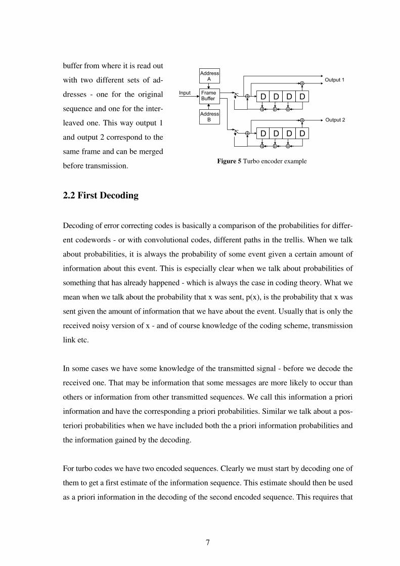
We will end this section by showing a more detailed drawing of a turbo encoder, Figure 5.

Here we see the two recursive systematic encoders, this time for the code

(1,(1+D )/(1+D+D +D +D )). Notice that the systematic bit is removed from one of them.4 2 3 4

At the input of the constituent encoders we see a switch. This is used to force the encoders

to the all-zero state - i.e. to terminate the trellis. The complete incoming frame is kept in a

7

Figure 5 Turbo encoder example

buffer from where it is read out

with two different sets of ad-

dresses - one for the original

sequence and one for the inter-

leaved one. This way output 1

and output 2 correspond to the

same frame and can be merged

before transmission.

2.2 First Decoding

Decoding of error correcting codes is basically a comparison of the probabilities for differ-

ent codewords - or with convolutional codes, different paths in the trellis. When we talk

about probabilities, it is always the probability of some event given a certain amount of

information about this event. This is especially clear when we talk about probabilities of

something that has already happened - which is always the case in coding theory. What we

mean when we talk about the probability that x was sent, p(x), is the probability that x was

sent given the amount of information that we have about the event. Usually that is only the

received noisy version of x - and of course knowledge of the coding scheme, transmission

link etc.

In some cases we have some knowledge of the transmitted signal - before we decode the

received one. That may be information that some messages are more likely to occur than

others or information from other transmitted sequences. We call this information a priori

information and have the corresponding a priori probabilities. Similar we talk about a pos-

teriori probabilities when we have included both the a priori information probabilities and

the information gained by the decoding.

For turbo codes we have two encoded sequences. Clearly we must start by decoding one of

them to get a first estimate of the information sequence. This estimate should then be used

as a priori information in the decoding of the second encoded sequence. This requires that

� (dt ) � logPr �dt�1 ,observation �

Pr �dt�0,observation �

� logPrap �dt�1 �

Prap�dt�0 �� log

Pr �observation�dt�1�

Pr �observation�dt�0�

� logPrap�dt�1 �

Prap�dt�0 �� �� (dt )

8

Figure 6 First decoding stage

(1)

the decoder is able to use a soft decision input and to produce some kind of soft output.

The decoding is sketched in Figure 6.

The standard decoder for turbo codes is the A Posteriori Probability decoding (APP)

(sometimes referred to as the Maximum A Posteriori decoding algorithm (MAP)). The

APP decoder, described in Section 3, does indeed calculate the a posteriori probabilities for

each information bits.

We will represent the soft input/output as log-likelihood ratios, i.e. a signed number where

negative numbers indicate that zero is the most likely value of the bit. As seen from For-

mula 1 the log-likelihood ratio of the a posteriori probabilities can easily be divided into

two components - the log- likelihood ratio of the a priori probabilities of the bit d and thet

information gained by the current observation. This means that when we gain additional

information about the information bits - like with the second decoding - we simply add a

(negative or positive) component to the log-likelihood ratio.

9

2.3 Putting Turbo on the Turbo Codes.

When we have a parity equation, it involves a number of information bits. Let us look at

one of the simplest possible parity equations - a sum of two information bits: P=I +I . It is1 2

clear that if both P and I are very reliable we get a reliable estimate of I , on the other2 1

hand if I is very unreliable we do not get much information about I . If we now imagine2 1

that both I and I are unreliable when we decoded the first sequence, but that I is in-1 2 2

volved in some parity equations with very reliable bits in the second encoded sequence -

then we might return to the parity equations from the first sequence for a second iteration

with this new and much more reliable estimate of I . This way we could continue to2

decode the two encoded sequences and iterate towards the final decision.

However, it is not that easy since we must be very careful not to use our information

more than once. Luckily we see from Formula 1, that it is easy to subtract the a priori

information - which came from the other decoder - from the decoder output. This will

prevent most of the unwanted positive feed-back. We may still have loops in the decision

process, though, i.e. we might see that I influences I in the first decoder, that I1 2 2

influences I in the second decoder and finally that I influences I in the next iteration in3 3 1

the first decoder. This way the new improved estimate of I will be based on information1

that came from I in the first place. 1

Use of the system in practice has shown that if we subtract the log-likelihood ratio of the a

priori information after each constituent decoder and make a number of decoding iterations

we get a system that is working remarkably well - for many applications it actually

outperforms the previously known systems. Still, we must conclude that the final result

after turbo decoding is a sub-optimal decoding due to the loops in the decision process. For

low signal-to-noise ratios we may even see that the decoding does not converge to anything

close to the transmitted codeword.

The turbo decoder is shown in Figure 7.

10

Figure 7 Turbo decoder

2.4 Performance Example

We will show an example of the performance with turbo codes. We use the system illus-

trated in Figure 5, i.e. the code (1,(1+D /(1+D+D +D +D ) for both encoders but the infor-4) 2 3 4

mation sequence is only transmitted from the first one. This means that the over-all rate is

1/3. The block length is 10384 bits and we use a pseudo-random interleaver. After each

frame the encoders are forced to the zero state. The corresponding termination tail - 4 in-

formation bits and 4 parity bits for each encoder, a total of 16 bits - is appended to the

transmitted frame and used in the decoder. In principle the termination reduces the rate, but

for large frames this has no practical influence. In this case the rate is reduced from 0.3333

to 0.3332.

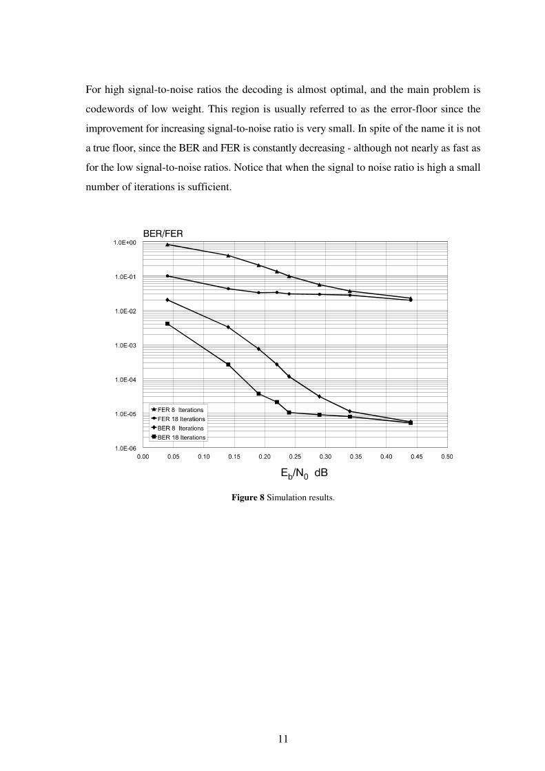
The performance curves for Bit Error Rate (BER) and Frame Error Rate (FER) are shown

in Figure 8. Due to the sub-optimal decoding the performance curves consist of two parts.

For low signal-to-noise ratios the main problem is lack of convergence in the iterated de-

coding process, resulting in frames with a large number of errors. In this region we are far

from optimal decoding. This means that we may benefit from more iterations. As we see

from the figure there is a considerable gain by going from 8 to 18 iterations, and with more

iterations the performance might be even better.

11

Figure 8 Simulation results.

For high signal-to-noise ratios the decoding is almost optimal, and the main problem is

codewords of low weight. This region is usually referred to as the error-floor since the

improvement for increasing signal-to-noise ratio is very small. In spite of the name it is not

a true floor, since the BER and FER is constantly decreasing - although not nearly as fast as

for the low signal-to-noise ratios. Notice that when the signal to noise ratio is high a small

number of iterations is sufficient.

Pr �Yt�Xt ���n

j�1

1

2���e

�(ytj�xtj)

2

2�2

Pr �St�1�m � ,St�m�Y L1 � �

Pr �St�1�m � ,St�m,Y L1 �

Pr�Y L1 �

, t�1...L

12

(2)

(3)

3. APP Decoding

The A Posteriori Probability (APP) algorithm does in fact calculate the a posteriori prob-

abilities of the transmitted information bits for a convolutional code. In this presentation

we will restrict ourselves to convolutional codes with rate 1/n.

The convolutional encoder with memory M (Figure 3) may be seen as a Markov source

with 2 states S , input d and output X . The output X and the new state S are functionsMt t tt t

of the input d and the previous state S .t t-1

If the output X is transmitted through a Discrete Memoryless Channel with white Gauss-t

ian noise. The probability of receiving Y when X was sent ist t

where x is the j-th bit of the transmitted word X , and y the corresponding receivedtj tjt

value. The signal to noise ratio is E /N =1/2� . In principle knowledge of the signal-to-s 02

noise ratio is needed for the APP algorithm. However, it may be chosen to a fixed value -

depending on the operation point of the system - with only a small degradation of the per-

formance.

Assume that we receive the sequence Y = Y ,Y ,...Y . The a posteriori probabilities of1 1 2 LL

the state transitions (i.e. branches) are found as:

Pr { Y } is a constant for a given received sequence and since we consider rate 1/n1L

codes only, there is one specific information bit associated with each state transition. We

therefore define

�t ( i ,m � )�Pr �dt�i ,St�1�m �,Y L1 �

� (dt ) � logPr �dt�1,observation �

Pr �dt�0,observation ��

�m �

�t(1 ,m � )

�m �

�t(0 ,m � )

�t (m)�Pr �St�m,Y t1 �

�t (m)�Pr �Y Lt����1�St�m �

�t ( i ,m � )�Pr �dt� i ,Yt�St�1�m � �

newstate( i ,m � )

oldstate(i,m)

Pr �Y Lt����1�St�m,Y t

1 ��Pr �Y Lt����1�St�m �

13

(4)

(5)

(6)

(7)

(8)

(11)

The final log-likelihood ratio becomes

In order to calculate � (i,m’) we define the following probability functions � (m), � (m),t t t

and � (i,m’) ast

Compared to the Viterbi algorithm � (m) corresponds to the state metrics, while � (i,m’)t t

corresponds to the branch metrics. � (m) can be seen as backwards state metrics.t

For the notation we will also need the function giving the new encoder state S when St t-1

= m’ and d =i t

and the function giving the old encoder state S when S =m and d =i t-1 t t

Since the encoder is a Markov process and the channel is memoryless, we have

and

�t ( i ,m � )�Pr �St�1�m � ,Y t����11 ��Pr �dt�i ,Yt�St�1�m � �

�Pr �Y Lt����1�St�newstate( i ,m � ) �

��t�1 (m �)��t( i ,m � )��t (newstate( i ,m � ))

�t (m)��i�0,1

Pr �dt� i ,St�1�oldstate(i ,m) ,Y t1 �

��i�0,1

Pr �St�1�oldstate(i ,m) ,Y t����11 ��Pr �dt� i ,Yt�St�1�oldstate(i ,m) �

��i�0,1

�t�1(oldstate(i ,m))��t ( i ,oldstate(i ,m))

�t (m)� �i�0,1

Pr �dt�1� i,Y Lt����1�St�m �

� �i�0,1

Pr �dt�1� i,Yt����1�St�m ��Pr �Y Lt����2�St�1�newstate(i,m) �

� �i�0,1

�t�1( i,m)��t�1(newstate( i ,m))

��

t (m) � Pr �St�m�Y t1 � �

Pr �St�m,Y t1 �

Pr �Y t1 �

�t (m)�Pr �St�m,Y t1 �

14

(12)

(13)

(14)

(15)

If we assume that the frames are terminated to state 0, we have � (0)=1, and � (m)= 0,0 0

m=1,2,...2 �1. We can calculate � as a forward recursionM

At the end of the frame we have � (0)=1, and � (m)=0, m=1,2,...2 �1. We can calculateL LM

� as a backward recursion

If the frames are not terminated we have no knowledge of the initial and final states. In

this case we must use � (m)= � (m)=2 .0 L-M

Since becomes very small with increasing t some rescaling must

be used. In principle the function �’ (m) should be usedt

where Pr{Y } is found as the sum of � (m) over all states, meaning that the �'(m) values1t

t t

always add up to one. However, since the output is the log-likelihood ratio the actual

�t (i,m� )�Prapriori �dt� i ��Pr �Yt�dt� i ,St�1�m � �

kt�1

Prapriori�dt�0 �

��

t (1,m � )�Prapriori �dt�1 �

Prapriori �dt�0 ��Pr �Yt�dt�1,St�1�m � �

��

t (0,m � )�Pr �Yt�dt�0,St�1�m � �

15

(16)

(17)

(18)

(19)

rescaling is not important as long as underflows are avoided. Similar the function � (m)t

needs rescaling.

The algorithm sketched here requires that � (m) is stored for the complete frame since wet

have to await the end of the frame before we can calculate � (m). We can instead use at

sliding window approach with period T and training period Tr. First � (m) is calculated andt

stored for t=0 to T-1. The calculation of � (m) is initiated at time t=T+Tr-1 with initialt

conditions � (m)=2 . The first Tr values � (m) is discarded but after the training pe-T+Tr-1 t-M

riod, i.e. for t=T-1 down to 0, we assume that � (m) is correct and ready for the calculationt

of � (i,m’). After the first window we continue with the next one until we reach the end oft

the frame where we use the true final conditions for � (m).L

Of course, this approach is an approximation but if the training period is carefully chosen

the performance degradation can be very small.

Since we have only one output associated with each transition, we can calculate � (i,m’) ast

For turbo codes the a priori information typically arrives as a log-likelihood ratio. Luckily

we see from the calculation of � (m) and � (m) that � (i,m’) is always used in pairs -t t t

� (0,m’) and � (1,m’). This means we can multiply � (i,m’) with a constant t t t

and get

x E y��log(e �x�e �y)�min(x ,y)�log(1�e �|y�x|)

16

(20)

For an actual implementation the values of � (m), � (m) and � (i,m’) may be represented ast t t

the negative logarithm to the actual probabilities. This is also common practice for Viterbi

decoders where the branch and state metrics are -log to the corresponding probabilities.

With the logarithmic presentation multiplication becomes addition and addition becomes

an E-operation, where

This function can be reduced to finding the minimum and adding a small correction factor.

As seen from Formula 18 the incoming log-likelihood ratio �’, can be used directly in the

calculation of -log(�) as the log-likelihood ratio of the a priori probabilities.

17

18

4. Final Remarks

This tutorial was meant as a first glimpse on the turbo codes and the iterated decoding

principle. Hopefully, we have shed some light on the topic, if there are still some dark spots

- try reading it again!

Of course there are a lot of details not explained here, a lot of variation to the turbo coding

scheme and a lot of things that may need a proof. Some of these can be found in the papers

on the literature list.

19

20

5. Selected Literature

[1] Jakob Dahl Andersen, “Turbo Codes Extended with Outer BCH Code”, Electron-

ics Letters, vol. 32 No. 22, Oct. 1996.

[2] J. Dahl Andersen and V. V. Zyablov, “Interleaver Design for Turbo Coding”,

Proc. Int. Symposium on Turbo Codes, Brest, Sept. 1997.

[3] Jakob Dahl Andersen, “Selection of Component Codes for Turbo Coding based

on Convergence Properties”, Annales des Telecommunication, Special issue on

iterated decoding, June 1999.

[4] L. R. Bahl, J. Cocke, F. Jelinek and R. Raviv, “ Optimal Decoding of Linear

Codes for Minimizing Symbol Error Rate,” IEEE Trans. Inform. Theory, vol IT-

20, pp 284-287, March 1974.

[5] S. Benedetto and G. Montorsi, “Performance Evaluation of Turbo-codes”, Elec-

tronics Letters, vol. 31, No. 3, Feb. 1995.

[6] S. Benedetto and G. Montorsi, “Serial Concatenation of Block And Convolutional

Codes”, Electronics Letters, Vol. 32, No. 10, May 1996.

[7] C. Berrou, A. Glavieux and P. Thitimajshima, “Near Shannon Limit Error-cor-

recting Coding and Decoding : Turbo-codes(1)”, Proc. ICC �93, pp. 1064-1070,

May 1993.

[8] C. Berrou and A. Glavieux, “Near Optimum Error Correcting Coding and Decod-

ing: Turbo Codes”, IEEE trans. on Communications, Vol. 44, No. 10, Oct. 1996.

[9] R. J. McEliece, E. R. Rodemich and J.-F. Cheng, “The Turbo Decision Algo-

rithm”, Presented at the 33rd Allerton Conference on Communication, Control

and Computing, Oct. 1995.

21

[10] L. C. Perez, J. Seghers and D. J. Costello, Jr, ”A Distance Spectrum Interpretation

of Turbo Codes”, IEEE Trans. on Inform. Theory, Vol. 42, No. 6, Nov. 1996.

[11] Steven S. Pietrobon, “Implementation and Performance of a Serial MAP Decoder

for use in an Iterative Turbo Decoder”, Proc. Int. Symposium on Information The-

ory, Whistler, Canada, Sept. 1995.