ctDiscrete

A Tractable Model of Buffer Stock Saving

August 7, 2011

Christopher D. Carroll1 Patrick Toche2

Abstract

In the spirit of Merton (1969) and Samuelson (1969), we present an analytically tractable modelof the effects of nonfinancial risk on intertemporal choice. Our simple framework can be adopted incontexts where modelers have, until now, chosen not to incorporate serious nonfinancial risk becauseavailable methods did not readily yield transparent insights. Our model produces an intuitive formulafor target assets, and we show how to analyze transition dynamics using a familiar Ramsey-style phasediagram. Despite its starkness, we argue that our model captures the key implications of nonfinancialrisk for intertemporal choice.

Keywords risk, uncertainty, precautionary saving, buffer stock saving

JEL codes C61, D11, E24

PDF: http://econ.jhu.edu/people/ccarroll/papers/ctDiscrete.pdfWeb: http://econ.jhu.edu/people/ccarroll/papers/ctDiscrete/

Archive: http://econ.jhu.edu/people/ccarroll/papers/ctDiscrete.zip(Contains Mathematica and Matlab code solving the model)

1Carroll: ccarroll@jhu.edu, Department of Economics, Johns Hopkins University, Baltimore Maryland 21218, USA; and NationalBureau of Economic Research. http://econ.jhu.edu/people/ccarroll 2Toche: ptoche@cityu.edu.hk, Department of Economicsand Finance, City University of Hong Kong, Tat Chee Avenue, Kowloon Tong, HK.

Thanks to several generations of Johns Hopkins University graduate students who helped correct many errors and infelicities in earlierversions of the material presented here.

1 IntroductionThe Merton-Samuelson model of portfolio choice is the foundation for the vast literatureanalyzing financial risk,1 not because it offers conclusions that cannot be obtained from otherframeworks,2 but because it is easy to use and its key insights emerge in a way that is natural,transparent, and intuitive — in a word, the Merton-Samuelson model is tractable.

Unfortunately, nonfinancial risk3 (which is much more important than financial risk formost households)4 has proven more difficult to analyze. Of course, a large and impressivenumerical literature has carefully computed the theoretical effects of realistically calibratednonfinancial risks in a variety of contexts.6 But because a formidable investment in humancapital is required to learn the computational methods necessary to solve such models, muchof the economic literature (and much graduate-level instruction) has dodged the question ofhow nonfinancial risk influences choices, by assuming perfect insurance markets or perfectforesight or risk neutrality or quadratic utility or Constant Absolute Risk Aversion, or byattempting only to match aggregate risks (which are orders of magnitude smaller than id-iosyncratic risks). These approaches rob the question of its essence, either by assuming thatmarkets transform nonfinancial risk into financial risk or by making implausible assumptionsin order to reach the implausible conclusion that decisions are largely or entirely unaffectedby such risk.7

Our paper’s contribution is to offer a tractable model that captures the key qualitativefeatures (and many quantitative features) of realistic models of the optimal response to nonfi-nancial risk, but without the customary technical difficulties. The model is a natural extensionof the no-risk perfect foresight framework. Its solution is characterized by simple, intuitiveequations and we show how the model’s results can be analyzed using a phase diagramanalysis that will be familiar to every student of the canonical Ramsey growth model taught ingraduate school.

The trick that yields tractability is to distill all nonreturn risk into a stark and simple pos-sibility: A one-time uninsurable permanent loss in nonfinancial income. For an individual’sdecision problem, this may be directly interpreted as the risk of a permanent transition intounemployment (or disability, or retirement). Our view is that the consumer’s response tothis single, tractable risk can capture most of the substantive essence (that is, the qualitative

1Merton (1969); Samuelson (1969); see Sethi and Thompson (2000) for an overview and extensions.2Merton and Samuelson cite the pioneering work of Markowitz (1959), Tobin (1958), and Phelps (1960) among others whose work had

already contained the key qualitative insights.3By which we mean risk that is both imperfectly insurable and imperfectly correlated with financial wealth.4Nonfinancial income typically accounts for the great majority of most households’ total income, while risky assets like stocks represent

a relatively small percentage of total wealth. Furthermore, stock returns are poorly correlated with the return on the index portfolio of allthe assets in the economy.5 Idiosyncratic risk is even more poorly spanned by market risk and is several orders of magnitude greater thanaggregate risk.

6The literature on in heterogeneous-agents macroeconomic models includes, among many others, Carroll (1992), Aiyagari (1994), andKrusell and Smith (1998), with roots that go back to Schechtman and Escudero (1977) and Bewley (1977), with other important contributionsby Clarida (1987), Zeldes (1989), and Chamberlain and Wilson (2000).

7The case of CARA utility with only labor income risk is included here because Carroll and Kimball (1996) show that it is a knife-edge case that is unrepresentative of the broader effects of uncertainty (notably, it fails to exhibit the consumption concavity that holdsfor virtually every other combination of assumptions); indeed, the addition of rate-of-return risk renders the optimal consumption functionconcave even under CARA utility. (The other traditional objection is that the optimal consumption plan under CARA utility generallyinvolves setting consumption to a negative value in some states of the world; it is hard to think of a plausible economic interpretation ofnegative consumption.)

2

and quantitative implications) of the results obtained in the numerical literature under morerealistic but more complex assumptions about income dynamics.

The same framework could be interpreted to apply in other contexts as well. For instance,the risk faced by a country whose exports are dominated by a commodity whose price mightcollapse permanently (e.g., oil exporters, if cold fusion had worked).8

The optimal response to such a risk is to aim to accumulate a buffer stock of precautionaryassets, as a form of “self-insurance.” The existing literature has found the numerical valueof the target under specific parametric assumptions, but has struggled to present an intuitivepicture of the determinants of that target. In contrast, we are able to derive an analyticalformula for the target level of wealth, and show transparently how the precautionary motiveinteracts with the other saving motives that have been well understood since Irving Fisher(1930)’s work: The income, substitution, and human wealth effects.

The literature’s principal alternative to numerical methods for analysis of precautionarybehavior has been to attempt to approximate the nonlinear part of the logarithmic consumptionEuler equation (the part that drives precautionary saving and the target level of assets). TheEuler equation approach, however, has foundered because the higher-level (beyond first-order)components of the Euler equation are endogenous in a way that has proven difficult to master.Thanks to our model’s tractability, we are able to derive a simple expression that shows howthe familiar perfect-foresight consumption Euler equation is modified by the presence of a one-shot risk. Specifically, our equation shows that the effect of the risk on consumption growthis related to the probability of the risky event, to its magnitude, to the consumer’s degree ofrisk aversion, and to the consumer’s wealth. We obtain an exact analytical expression (not alog-linearized one) for the combined value of the higher-order terms at the target. With thisexpression in hand, the intuition comes into clear focus, and the problems that have bedeviledthe literature can be plainly articulated and understood.

Our hope is that tractability of this kind will eventually allow a model like ours to becomethe standard reference point to which more specialized models can be compared in much ofeconomics, replacing the perfect foresight, certainty equivalent, or perfect markets modelsthat are currently so widely used because of their own tractability. A further ambition isthat even the specialist literatures like heterogeneous-agents macroeconomics may find ours auseful ‘toy model’ with which to exposit more clearly some of the subtle points that authors inthose literatures find difficult to communicate simply by appealing to results from numericalsimulations.9

8 The model could even be interpreted as applying to the behavior of a firm controlled by a risk-neutral manager, so long as the collapseof a line of business could have the effect of reducing the firm’s collateral value and therefore increasing its cost of external finance a laBernanke, Gertler, and Gilchrist (1996). In this case, the convex increase in borrowing rates when cash drops plays the same role as theconvexity of the marginal utility function for a consumer; see also Berk, Stanton, and Zechner (2009) for an argument that senior firmmanagers are not risk neutral even if shareholders are, because poor performance under their tenure will reduce their own future employmentopportunities. A firm controlled by such managers may behave very much like a risk-averse household.

9In order to assist authors in modifying our model for other purposes, we have constructed a public archive that contains Matlab andMathematica programs that produce all the results and figures reported in this paper, along with some other examples of uses to which themodel could be put. The archive is available on the first author’s website.

3

2 The Decision ProblemFor concreteness, we analyze the problem of an individual consumer facing a labor incomerisk. Other interpretations (like the ones mentioned in the introduction) are left for futurework or other authors. We couch the problem in discrete time, but in most cases we providethe logarithmic approximations that will correspond to the exact solution to the correspondingproblem in continuous time.10

The aggregate wage rate, Wt, grows by a constant factor G from the current time period tothe next, reflecting exogenous productivity growth:

Wt+1 = GWt. (1)

The interest rate is exogenous and constant (the economy is small and open); the interestfactor is denoted R.11 Define mmm as market resources (financial wealth plus current income),aaa as end-of-period assets after all actions have been accomplished (specifically, after theconsumption decision), and bbb as bank balances before receipt of labor income. Individualsare subject to a dynamic budget constraint (DBC) that can be decomposed into the followingelements:

aaat = mmmt − ccct (2)bbbt+1 = Raaat (3)mmmt+1 = bbbt+1 + `t+1Wt+1ξt+1 (4)

where ` measures the consumer’s labor productivity (hours of work for an employed consumerare assumed to be exogenous and fixed) and ξ is a dummy variable indicating the consumer’semployment state: Everyone in this economy is either employed (ξ = 1, a state indicated bythe letter ‘e’) or unemployed (ξ = 0, a state indicated by ‘u’). Thus, labor income is zero forunemployed consumers.12

2.1 The Unemployed Consumer’s Problem

There is no way out of unemployment; once an individual becomes unemployed, that indi-vidual remains unemployed forever, ξt = 0=⇒ξt+1 = 0 ∀ t. Consumers have a CRRA utilityfunction u(•) = •1−ρ/(1 − ρ), with ρ > 1, and they discount future utility geometrically by βper period. We show below that the simplicity of the unemployed consumer’s behavior is whatmakes employed consumer’s problem tractable. The solution to the unemployed consumer’soptimization problem is simply:13

cccut = κubbbt, (5)

10See Toche (2005) for an explicit but brief treatment of a closely related model in continuous time.11General equilibrium is not much more difficult; it requires specifying a production function and finding the level of capital for which

the optimal level of saving is zero (net of depreciation). Little further insight is obtained, while many potential extra sources of confusion areadded.

12This is without loss of generality. We could allow for unemployment insurance by modifying the value of ξ associated withunemployment. On this, see also footnote 4 in Toche (2005).

13This is a standard result, which follows from the first-order condition and the budget constraint:

u′(cccut ) = Rβu′(cccu

t+1)⇒(cccu

t)−ρ

= Rβ(cccu

t+1

)−ρ⇒ cccu

t+1 = (Rβ)1/ρ cccut .

4

where κu is the ‘marginal propensity to consume’ out of total wealth (MPC), which for theunemployed consists in balances bbb only.

2.1.1 Parameter Restrictions

Table 1 summarizes our notation and should serve as a useful guide to the reader. We followthe terminology in Carroll (2011), where a detailed discussion of the concepts is provided.The marginal propensity to consume out of total wealth κu is related to the ‘return patiencefactor’ ÞÞÞR as follows14

κu = 1 −ÞÞÞR, ÞÞÞR ≡ R−1(Rβ)1/ρ. (6)

The MPC for the problem without risk is strictly below the MPC for the problem with risk(Carroll and Kimball, 1996). We impose a ‘return impatience condition’ (RIC),

ÞÞÞR < 1⇒ κu > 0, (7)

The interpretation is that the consumer must not be so patient that a boost to total wealthwould fail to boost current consumption.15 An alternative (equally correct) interpretation isthat the condition guarantees that the present discounted value (PDV) of consumption for theunemployed consumer remains finite. ÞÞÞR is the ‘return patience factor’ because it definesdesired perfect-foresight consumption growth relative to the rate of return R. We define the‘return patience rate’ as the lower-case version:

þr ≡ logÞÞÞR ≈ ÞÞÞR − 1 = −κu.

For short, we will sometimes say that a consumer is ‘return impatient’ (or, ‘the RIC holds’)if ÞÞÞR < 1 or if þr < 0 or if κu > 0, all three conditions being equivalent.16 A consumer who isreturn impatient is someone who will be spending enough to make the ratio of consumptionto total wealth decline over time.

The return patience factor can be compared to the ‘absolute patience factor’

ÞÞÞ = (Rβ)1/ρ (8)

which is the growth factor for consumption in the no-risk perfect foresight model. We say thata consumer is ‘absolutely impatient’ if

ÞÞÞ < 1, (9)

in which case the consumer will choose to spend more than the amount that would permitconstant consumption; such a consumer’s absolute level of wealth declines over time, and

Consumption grows at the geometric rate (Rβ)1/ρ. The present discounted value of consumption at time t must equal total wealth, so that

∞∑i=0

R−icccut+i =

∞∑i=0

R−i (Rβ)i/ρ cccut =

∞∑i=0

(1 − κu)icccut = cccu

t /κu = bbbt .

14ÞÞÞ is the Old English letter ‘thorn’; its modern equivalent is the digraph ‘th.’15‘Pathologically patient’ consumers who do not satisfy this condition would hoard any increase in wealth in order to enable even more

extra consumption in the distant future.16Throughout, we casually treat logs of factors like ÞÞÞR as equivalent to the level minus 1; that is, we treat expressions like logÞÞÞR and

ÞÞÞR − 1 as interchangeable, which is an appropriate approximation so long as the factor is ‘close’ to 1. In practice, the approximation is verygood.

5

therefore consumption itself declines, since consumption is proportional to total wealth. Anal-ogously to (8), we define the absolute patience rate as

þ ≡ logÞÞÞ ≈ ρ−1(r − ϑ). (10)

2.2 The Employed Consumer’s Problem

The consumer’s preferences are the same in the employment and unemployment states; onlyexposure to risk differs.

2.2.1 A Human-Wealth-Preserving Spread in Unemployment Risk

A consumer who is employed in the current period has ξt = 1; if this person is still employednext period (ξt+1 = 1), market resources will be:

mmmet+1 = (mmme

t − cccet )R + Wt+1`t+1. (11)

However, there is no guarantee that the consumer will remain employed: Employed consumersface a constant risk f of becoming unemployed. It is convenient to define f ≡ 1 − f, thecomplementary probability that a consumer does not become unemployed. We assume that `grows by a factorf−1 every period,

`t+1 = `t/f, (12)

because under this assumption, for a consumer who remains employed, labor income will growby factor Γ = G/f, so that the expected labor income growth factor for employed consumersis the same G as in the no-risk perfect foresight case:

Et[Wt+1`t+1ξt+1] =

(`tGWt

f

) (f × 0 +f × 1

)⇒Et[Wt+1`t+1ξt+1]

Wt`t= G

implying that an increase in f is a pure increase in risk with no effect on the PDV of expectedlabor income – a mean-preserving spread in the intertemporal sense. Thus, any change inbehavior that results from a change in f will be cleanly interpretable as reflecting an effect ofuncertainty rather than the effect of a change in human wealth.

2.2.2 First Order Optimality Condition

The usual steps lead to the standard consumption Euler equation. Using i ∈ e, u to stand forthe two possible states,

u′(cccet ) = RβEt

[u′(ccci

t+1)]

⇒ 1 = RβEt

(cccit+1

cccet

)−ρ . (13)

Henceforth nonbold variables will be used to represent the bold equivalent divided by thelevel of permanent labor income for an employed consumer, e.g. ce

t = cccet /(Wt`t); thus we can

6

rewrite the consumption Euler equation as:

1 = RβEt

(cit+1Wt+1`t+1

cet Wt`t

)−ρ⇒ = RβEt

(cit+1

cet

Γ

)−ρ⇒ = Γ−ρRβ

(1 −f)

(ce

t+1

cet

)−ρ+f

(cu

t+1

cet

)−ρ, (14)

where the term in braces is a probability-weighted average of the growth rates of marginalutility in the case where the consumer remains employed (the first term) and the case wherethe consumer becomes unemployed (the second term).

2.2.3 Analysis and Intuition of Consumption Growth Path

It will be useful now to define a ‘growth patience factor’ ÞÞÞΓ = (Rβ)1/ρ/Γ which is the factorby which the consumption-income ratio ce would grow in the absence of labor income risk.With this notation, (14) can be written as:

1 = ÞÞÞρΓ

(ce

t+1

cet

)−ρ 1 −f +f

[(cu

t+1

cet

) (ce

t

cet+1

)]−ρ⇒

(ce

t+1

cet

)= ÞÞÞΓ

1 +f

[(ce

t+1

cut+1

)ρ− 1

]1/ρ

. (15)

To understand (15), it is useful to consider an approximation. Define ∇t+1 ≡

(ce

t+1−cut+1

cut+1

), the

proportion by which consumption next period would drop in the event of a transition intounemployment; we refer to this loosely as the size of the ‘consumption risk.’ Define ω, the‘excess prudence’ factor, as ω = (ρ − 1)/2.17 Applying a Taylor approximation to (15) (seeappendix A) yields: (

cet+1

cet

)≈ (1 +f(1 + ω∇t+1)∇t+1)ÞÞÞΓ (16)

which simplifies further in the logarithmic utility case (since ρ = 1 and thus ω = 0),(ce

t+1

cet

)≈ (1 +f∇t+1)ÞÞÞΓ. (17)

The approximations in (16) or (17) capture the essence of equation (15). As a consequenceof missing insurance markets, consumption growth depends on the employment outcome;18

consumption if employed next period cet+1 is greater than consumption if unemployed next

period cut+1, so that ∇t+1 is positive. In the limit case, as unemployment risk f vanishes, so

17It is ‘excess’ in the sense of exceeding the benchmark case of logarithmic utility which corresponds to ρ = 1. Logarithmic utility isoften viewed as a lower bound on the possible degree of risk aversion.

18Markets are incomplete by assumption. The no-slavery provisions of the U.S. Constitution prohibit even indentured servitude,providing a moral hazard explanation for why this insurance market should be missing. Adverse selection arguments provide an evenbetter explanation.

7

does consumption risk ∇,19 and thus cet+1/c

et approaches ÞÞÞΓ. Equation (16) thus shows that the

presence of unemployment risk boosts consumption growth by an amount proportional to theprobability of becoming unemployed f multiplied by a factor that is increasing in the amountof consumption risk ∇. In the logarithmic case, equation (17) shows that the precautionaryboost to consumption growth is directly proportional to the size of the consumption risk.

The effect of risk on saving is transparent. For a given value of met , risk has no effect on

the PDV of future labor income and human wealth, but the larger is f, the faster consumptiongrowth must be, as equation (16) shows. For consumption growth to be faster while keepingthe PDV constant, the level of current ce must be lower. Thus, the introduction of a risk ofunemployment f induces a (precautionary) increase in saving.

In the (persuasive) case where ρ > 1, (16) implies that a consumer with a higher degree ofprudence (larger ρ and therefore larger ω) will anticipate greater consumption growth. Thisreflects the greater precautionary saving motive induced by a higher degree of prudence.

To compute the steady state of the model, we must find the ∆cet+1 = 0 and ∆me

t+1 = 0 loci.Consider a consumer who is unemployed in period t+1. Dividing both sides of (4) by Wt+1`t+1

yields mut+1 = bu

t+1 = (met − ce

t )R (where R ≡ R/Γ). Substituting cet+1 = ce

t and cut+1 = κumu

t+1into (15) yields:

1 =

1 +f

[(ce

t+1

κumut+1

)ρ− 1

]ÞÞÞρ

Γ

⇒ce

t+1

(met − ce

t )Rκu =

ÞÞÞ−ρΓ−f

f

1/ρ

≡ Π

⇒ cet+1 = (me

t − cet )Rκ

uΠ (18)

where the expression mut+1 = (me

t − cet )R has been used in the second line.

We now turn to parameter restrictions necessary to guarantee a positive steady state.

2.2.4 Parameter Restrictions (Continued)

Consider equation (18). We know that met > ce

t > 0 because, with CRRA preferences, zeroconsumption carries an infinite penalty, implying that a consumer facing the risk of perpetualunemployment will never borrow. Since we have assumed κu > 0 (the RIC), steady-stateconsumption is positive only if Π is positive; so we impose the condition

ÞÞÞΓ < (1 −f)−1/ρ. (19)

In the limit as f approaches zero, (19) therefore reduces to a requirement that the growthpatience factor ÞÞÞΓ be less than one,

ÞÞÞΓ < 1. (20)

Following Carroll (2011), we call condition (20) the ‘perfect foresight growth impatiencecondition’ (PF-GIC), by analogy with the ‘return impatience condition’ (7) imposed earlier.If f = 0, the consumer knows with perfect certainty what will happen in the future; the PF-

19While unemployment risk f is exogenous, consumption risk ∇ is endogenous.

8

GIC ensures that such a consumer facing no risk would be sufficiently impatient to choose awealth-to-permanent-income ratio that would be falling over time.20,21

Using γ ≡ log Γ, we similarly define the corresponding ‘growth patience rate’

þγ ≡ logÞÞÞΓ (21)

so that the PF-GIC can also be written

þγ ≈ ρ−1(r − ϑ) − γ < 0. (22)

2.2.5 Why Increased Unemployment Risk Increases Growth Impatience

Under the maintained assumption that the RIC holds, the (generalized) GIC in (19) slackens(becomes easier to satisfy) as unemployment risk rises because, with relative risk aversionρ > 1, an increase in f reduces the right-hand side of (19). This occurs for two reasons.First, an increase in f is like a reduction in the future downweighting factor (that is, adecrease in patience), conditional on the consumer remaining employed.22 Second, an increasein f slackens the GIC because our mean-preserving-spread assumption requires that laborproductivity growth be adjusted so that the value of human wealth is independent of f –see (12). The higher f is, the faster growth is conditional on remaining employed. Asincome growth (conditional on employment) increases, the continuously-employed (lucky)consumer is effectively more ‘impatient’ in the sense of desiring consumption growth belowemployment-conditional income growth.23

The fact that the GIC is easier to satisfy as f increases means that if the PF-GIC (20) issatisfied, then (19) must be satisfied.

2.2.6 The Target Level of me

We first characterize the steady state. Setting ∆cet+1 = 0 and ∆me

t+1 = 0 yields, respectively

cet =

(RκuΠ

1 + RκuΠ

)me

t (23)

= (1 − R−1)met + R−1. (24)

Equation (23) is obtained by imposing the RIC and the GIC on (18). Equation (24) followsfrom normalizing the DBC in (11).

The steady-state levels of me and ce are the values for which both (24) and (23) hold. Thissystem of two equations in two unknowns can be solved explicitly (see the appendix). Forillustration, consider the special case of logarithmic utility (ρ = 1). The appendix shows that

20The PF-GIC is a slightly stronger condition than is strictly necessary; the necessary condition is (19). However, the PF-GIC guaranteesthat the solution is well behaved as the risk vanishes, which lends itself to a more intuitive interpretation.

21 In addition, the condition met > 0 suggests the condition RκuΠ > 1 − R. This follows from (34) below. It is equivalent to Π =

cet+1/c

ut+1 > ((1 − R)/R)/κu, i.e. the marginal propensity to consume in the unemployment state must be sufficiently small. The appendix

shows that this condition is automatically satisfied if the RIC and GIC are imposed, thus no additional restrictions are needed to guaranteepositive wealth in the state of unemployment.

22While this effect is offset by an increase in the downweighting factor associated with the transition to the unemployed state, the RICalready guarantees that the PDV of consumption, income, and value remain finite for the unemployed consumer, who is therefore irrelevant.

23Note that neither of these effects of f is precautionary.

9

an approximation of the target level of market resources is

me ≈ 1 +

(1

(γ − r) + ϑ(1 + (γ + ϑ − r)/f)

). (25)

The GIC and the RIC together guarantee that the denominator of (25) is positive.This expression encapsulates several of the key intuitions of the model. The human wealth

effect of labor income growth (conditional upon remaining employed) is captured by the first γterm in the denominator; for any calibration for which the denominator is positive, increasingγ reduces the target level of wealth. This reflects the fact that a consumer who anticipatesbeing richer in the future will choose to save less in the present, and the result of lower savingis smaller wealth. The human wealth effect of interest rates is correspondingly captured bythe −r term, which goes in the opposite direction to the effect of income growth, because anincrease in the rate at which future labor income is discounted constitutes a reduction in humanwealth. An increase in the rate at which future utility is discounted, ϑ, reduces the target wealthlevel. Finally, a reduction in unemployment risk raises (γ+ϑ− r)/f and therefore reduces thetarget wealth level.24,25

Note that the different effects interact with each other, in the sense that the strength of,say, the human wealth effect of interest rates will vary depending on the values of the otherparameters.

The assumption of log utility is implausible; empirical estimates from structural estimationexercises (e.g. Gourinchas and Parker (2002), Cagetti (2003), or the subsequent literature)typically find estimates considerably in excess of ρ = 1, and evidence from Barsky, Juster,Kimball, and Shapiro (1997) suggests that values of 5 or higher are not implausible. Anotherspecial case helps to illuminate how results change for ρ > 1. The appendix shows that, in thespecial case where ϑ = r, the target level of wealth is:

m ≈ 1 +

(1

(γ − r) + ϑ(1 + (γ/f)(1 − (γ/f)ω))

). (26)

Compare the target level in (26) with (25). The key difference is that (26) contains an extraterm involving ω, which measures the amount by which prudence exceeds the logarithmicbenchmark. An increase in ω reduces the denominator of (26) and thereby raises the targetlevel of wealth, just as would be expected from an increase in the intensity of the precautionarymotive.

In the ω > 0 case, the interaction effects between parameter values are particularly intensefor the (γ/f)2 term that multiplies ω; this implies, e.g., that a given increase in unemploymentrisk can have a greater effect on the target level of wealth for a consumer who is more prudent.

10

Figure 1 Phase Diagram

Dct+1e =0

Dmt+1e = 0

Stable Arm

SS

mte

cte

2.2.7 The Phase Diagram

Figure 1 presents the phase diagram of system (23)-(24) under our baseline parameter values.Since the employed consumer never borrows, market resources never fall below the value ofcurrent labor income, which is the value selected for the origin of the diagram.26 An intuitiveinterpretation is that the ∆me

t = 0 locus characterized by (24) shows how much consumption cet

would be required to leave resources met unchanged so that me

t = met .

27 Thus, any point belowthe ∆me

t = 0 line would have consumption below the break-even amount, implying that wealthwould rise. Conversely for points above ∆me

t = 0. This is the logic behind the horizontalarrows of motion in the diagram: Above ∆me

t = 0 the arrows point leftward, below ∆met = 0

the arrows point rightward.The intuitive interpretation of the ∆ce

t = 0 locus characterized by (23) is more subtle. Recallthat expected consumption growth depends on the amount by which consumption would fallif the unemployment state were realized. At a given level of resources, the farther actualconsumption (if employed) is below the break-even (sustainable) amount, the smaller the ce

t /cut

ratio is, and therefore the smaller consumption growth is. Points below the ∆cet = 0 locus are

24(γ + ϑ − r) > 0 is guaranteed by (22) under log utility (ρ = 1).25This discussion omits the fact that an increase in f requires an adjustment to γ via (12) which induces a human wealth effect that goes

in the opposite direction from the direct effect of uncertainty. For sufficiently large values of f, this effect can dominate the direct effect ofuncertainty and the target wealth-to-income ratio declines. See the illustration below of the effects of an increase in uncertainty for furtherdiscussion. The same qualitative results may be found by a direct analysis of the partial derivatives of equation (34).

26Our parameterization is not indended to maximize realism, but instead to generate well-proportioned figures that illustrate themechanisms of the model as clearly as possible. The parameter values are encapsulated in the file ParametersBase.m in the online archive.

27Some authors refer to ∆met = 0 as the level of ‘permanent income.’ However, this definition differs from Friedman (1957)’s and,

moreover, is a potential source of confusion with permanent labor income’ Wt`t; we prefer to describe the locus as depicting the level of‘sustainable consumption.’

11

Figure 2 The Consumption Function for the Employed Consumer

45 Degree Line

Consumption Function cHmteL

cHmteLPerf Foresight

mte

cte

associated with negative values of ∆cet . This is the logic behind the vertical arrows of motion

in the diagram: Above ∆cet = 0 the arrows point upward, below ∆ce

t = 0 the arrows pointdownward.

2.2.8 The Consumption Function

Figure 2 shows the optimal consumption function c(m) for an employed consumer (droppingthe e superscript to reduce clutter). This is of course the stable arm of the phase diagram. Alsoplotted are the 45 degree line along which ct = mt and

c(m) = (m − 1 + h)κu, (27)

where

h =

(1

1 − G/R

)(28)

is the level of (normalized) human wealth. c(m) is the solution to the no-risk version of themodel; it is depicted in order to introduce another property of the model: As wealth approachesinfinity, the solution to the problem with risky labor income approaches the solution to the no-risk problem arbitrarily closely.28,29

The consumption function c(m) is concave: The marginal propensity to consume κκκ(m) ≡dc(m)/dm is higher at low levels of m because the intensity of the precautionary motive

28This limiting result requires that we impose the additional assumption Γ < R, because the no-risk consumption function is not definedif Γ ≥ R.

29If the horizontal axis is stretched far enough, the two consumption functions appear to merge (visually), with the 45 degree linemerging (visually) with the vertical axis. The current scaling is chosen both for clarity and to show realistic values of wealth.

12

increases as resources m decline.30 The MPC is higher at lower levels of m because therelaxation in the intensity of the precautionary motive induced by a small increase in m(Kimball, 1990) is relatively larger for a consumer who starts with less than for a consumerwho starts with more resources (Carroll and Kimball, 1996).

To see this important point, consider a counterfactual. Suppose the consumer were to spendall his resources in period t, i.e. ct = mt. In this situation, if the consumer were to becomeunemployed in the next period, he would then be left with resources mu

t+1 = (mt − ct)R = 0,which would induce consumption cu

t+1 = κumut+1 = 0, yielding negative infinite utility. A

rational, optimizing consumer will always avoid such an eventuality, no matter how small itslikelihood may be. Thus the consumer never spends all available resources.31 This implicationis illustrated in figure 2 by the fact that consumption function always remains below the 45degree line.

2.2.9 Expected Consumption Growth Is Downward Sloping in me

Figure 3 illustrates some of the key points in a different way. It depicts the growth rate ofconsumption ccce

t+1/cccet as a function of me

t .Figure 3 illustrates the result that consumption growth is equal to what it would be in the

absence of risk, plus a precautionary term; for algebraic verification, multiply both sides of(15) by Γ to obtain (

cccet+1

cccet

)= (Rβ)1/ρ

1 +f

[(ce

t+1

cut+1

)ρ− 1

]1/ρ

, (29)

and observe that the contribution of the precautionary motive becomes arbitrarily large asmt → 0, because cu

t+1 = mut+1κ

u = (mt − c(mt))Rκu approaches zero as mt → 0; that is, asresources me

t decline, expected consumption growth approaches infinity. The point whereconsumption growth is equal to income growth is at the target value of me.

2.2.10 Summing Up the Intuition

We are finally in position to get an intuitive understanding of how the model works and whya target wealth ratio exists. On the one hand, consumers are growth-impatient: It cannot beoptimal for them to let wealth become arbitrarily large in relation to income. On the otherhand, consumers have a precautionary motive that intensifies as the level of wealth falls. Thetwo effects work in opposite directions. As resources fall, the precautionary motive becomesstronger, eventually offsetting the impatience motive. The point at which prudence becomesexactly large enough to match impatience defines the target wealth-to-income ratio.

It is instructive to work through a couple of comparative dynamics exercises. In doing so, weassume that all changes to the parameters are exogenous, unexpected, and permanent. Figure 4depicts the effects of increasing the interest rate to r > r. The no-risk consumption growthlocus shifts up to the higher value þr ≈ ρ

−1(r − ϑ), inducing a corresponding increase in the

30Carroll and Kimball (1996) prove that the consumption function must be concave for a general class of stochastic processes and utilityfunctions – including almost all commonly-used model assumptions except for the knife-edge cases explicitly chosen to avoid concavity.

31This is an implication not just of the CRRA utility function used here but of the general class of continuously differentiable utilityfunctions that satisfy the Inada condition u′(0) = ∞.

13

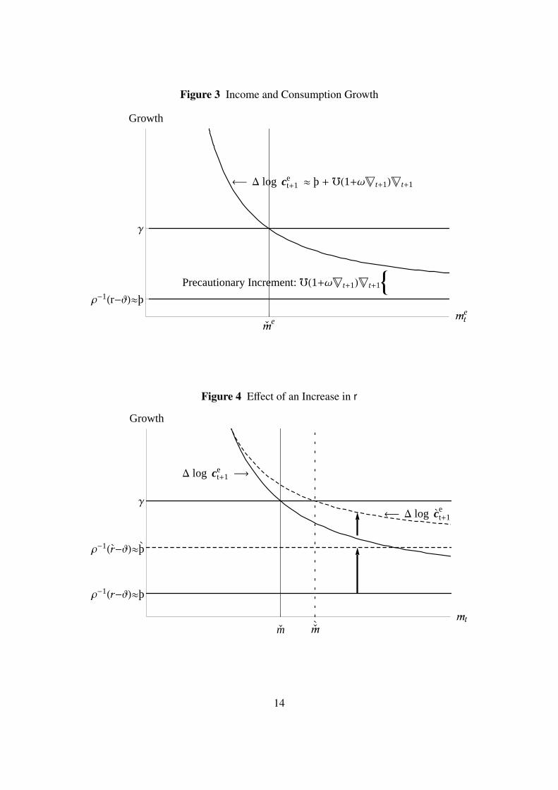
Figure 3 Income and Consumption Growth

D log ct+1e » þ + °H1+Ω!t+1L!t+1

8Precautionary Increment: °H1+Ω!t+1L!t+1

mÇ emt

e

Γ

Ρ-1Hr-JL»þ

Growth

Figure 4 Effect of an Increase in r

D log c t+1e

D log ct+1e

mÇ mÇ mt

Γ

Ρ-1Hr-JL»þ

Ρ-1Hr-JL»þ

Growth

14

Figure 5 Effect of an Increase in Unemployment Risk f to f

D log c t+1e

Original Eqbm

New Target

mÇ mÇ mt

ΓΓ

Ρ-1Hr-JL»þ

Growth

expected consumption growth locus. Since the expected growth rate of labor income remainsunchanged, the new target level of resources `me is higher. Thus, an increase in the interest rateraises the target level of wealth, an intuitive result that carries over to more elaborate models ofbuffer-stock saving with more realistic assumptions about the income process (Carroll (2011)).

The next exercise is an increase in the risk of unemployment f. The principal effect weare interested in is the upward shift in the expected consumption growth locus to ∆ccct+1. If thehousehold starts at the original target level of resources m, the size of the upward shift at thatpoint is captured by the arrow orginating at m, γ.

In the absence of other consequences of the rise in f, the effect on the target level ofm would be unambiguously positive. However, recall our adjustment to the growth rateconditional upon employment, (12); this induces the shift in the income growth locus to γwhich has an offsetting effect on the target m ratio. Under our benchmark parameter values,the target value of m is higher than before the increase in risk even after accounting for theeffect of higher γ, but in principle it is possible for the γ effect to dominate the direct effect.Note, however, that even if the target value of m is lower, it is possible that the saving ratewill be higher; this is possible because the faster rate of γ makes a given saving rate translateinto a lower ratio of wealth to income. In any case, our view is that most useful calibrationsof the model are those for which an increase in uncertainty results in either an increase inthe saving rate or an increase in the target ratio of resources to permanent income. This ispartly because our intent is to use the model to illustate the general features of precautionarybehavior, including the qualitative effects of an increase in the magnitude of transitory shocks,which unambiguously increase both target m and saving rates.

15

2.2.11 Death to the Log-Linearized Consumption Euler Equation!

Our simple model may help explain why the attempt to estimate preference parameters like thedegree of relative risk aversion or the time preference rate using consumption Euler equationshas been so signally unsuccessful (Carroll (2001)). On the one hand, as illustrated in figures 3and 4, the steady state growth rate of consumption, for impatient consumers, is equal to thesteady-state growth rate of income,

∆ log cccet+1 = γ. (30)

On the other hand, under logarithmic utility our approximation of the Euler equation forconsumption growth, obtained from equation (29), seems to tell a different story,

∆ log cccet+1 ≈ þ +f∇t+1, (31)

where the last line uses the Taylor approximations used to obtain (16). The approximate Eulerequation (31) does not contain any term explicitly involving income growth. How can wereconcile (30) and (31) and resolve the apparent contradiction? The answer is that the size ofthe precautionary term f∇t+1 is endogenous (and depends on γ). To see this, solve (30)- (31):In steady-state,

f∇ ≈ γ − þ. (32)

The expression in (32) helps to understand the relationship between the model parameters andthe steady-state level of wealth. From figure 3 it is apparent that ∇t+1(me

t ) is a downward-sloping function of me

t . At low levels of current wealth, much of the spending of an employedconsumer is financed by current income. In the event of job loss, such a consumer must suffera large drop in consumption, implying a large value of ∇t+1.

To illustrate further the workings of the model, consider an increase in the growth rateof income. On the one hand, the right-hand side of (32) rises. But, lower wealth raisesconsumption risk, so that the new target level of m must be lower, and this raises the left-handside of (32). In equilibrium, both sides of the expression rise by the same amount.

The fact that consumption growth equals income growth in the steady-state poses majorproblems for empirical attempts to estimate the Euler equation. To see why, suppose we hada collection of countries indexed by i, identical in all respects except that they have differentinterest rates ri. In the spirit of Hall (1988), one might be tempted to estimate an equation ofthe form

∆ log ccci = η0 + η1ri + ε i, (33)

and to interpret the coefficient on ri as an empirical estimate of the value of ρ−1. This empiricalstrategy will fail. To see why, consider the following stylized scenario. Suppose that all thecountries are inhabited by impatient workers with optimal buffer-stock target rules, but eachcountry has a different after-tax interest rate (measured by ri. Suppose that the workers are notfar from their wealth-to-income target, so that ∆ logccci = γi. Suppose further that all countrieshave the same steady-state income growth rate and the same unemployment rate.32

32The key point holds if countries have different growth rates; this stylized example is merely an illustration.

16

A regression of the form of (33) would return the estimates

η0 = γ

η1 = 0.

The regression specification suffers from an omitted variable bias caused by the influence ofthe (endogenous) f∇i term. In our scenario, the omitted term is correlated with the includedvariable ri (and if our scenario is exact, the correlation is perfect). Thus, estimates obtainedfrom the log-linearized Euler equation specification in (33) will be biased estimates of ρ−1. Fora thorough discussion of this econometric problem, see Carroll (2001). For a demonstrationthat the problem is of pratical importance in (macroeconomic) empirical studies, see Parkerand Preston (2005).

2.2.12 Dynamics Following An Increase in Patience

We now consider a final experiment: Figure 6 depicts the effect on consumption of a decreasein the rate of time preference (the change is exogenous, unexpected, permanent), startingfrom a steady-state position. A decrease in the discount rate (an increase in patience) causesan immediate drop in the level of consumption; successive points in time are reflected in theseries of dots in the diagram. The new consumption path (or consumption function) starts froma lower consumption level and has a higher consumption growth than before the decrease inϑ.33

Consumption eventually approaches the new, higher equilibrium target level. This higherlevel of consumption is financed, in the long run, by the higher interest income provided bythe higher target level of wealth.

Note again, however, that equilibrium steady-state consumption growth is still equal to thegrowth rate of income (this follows from the fact that there is a steady-state level for the ratioof consumption to income). The higher target level of the wealth-to-income ratio is preciselyenough to reduce the precautionary term by an amount that exactly offsets the effect of the risein −ρ−1ϑ.

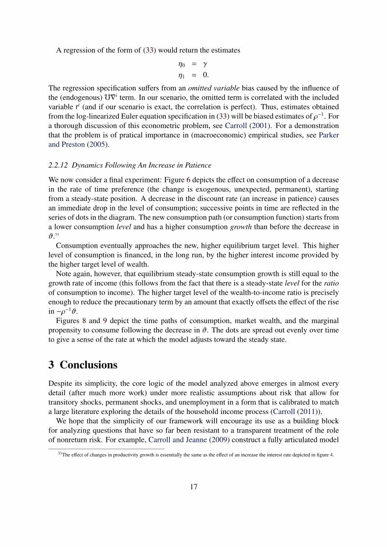
Figures 8 and 9 depict the time paths of consumption, market wealth, and the marginalpropensity to consume following the decrease in ϑ. The dots are spread out evenly over timeto give a sense of the rate at which the model adjusts toward the steady state.

3 ConclusionsDespite its simplicity, the core logic of the model analyzed above emerges in almost everydetail (after much more work) under more realistic assumptions about risk that allow fortransitory shocks, permanent shocks, and unemployment in a form that is calibrated to matcha large literature exploring the details of the household income process (Carroll (2011)).

We hope that the simplicity of our framework will encourage its use as a building blockfor analyzing questions that have so far been resistant to a transparent treatment of the roleof nonreturn risk. For example, Carroll and Jeanne (2009) construct a fully articulated model

33The effect of changes in productivity growth is essentially the same as the effect of an increase the interest rate depicted in figure 4.

17

Figure 6 Effect of Lower ϑ On Consumption Function

Orig Target New Target

Orig cHmL

New cHmL

m

c

of international capital mobility for a small open economy using the model analyzed here asthe core element. We can envision a variety of other direct purposes the model could serve,including applications to topical questions such as the effects of risk in a search model ofunemployment.

18

Figure 7 Path of ce Before and After ϑ Decline

0Time

cte

Figure 8 Path of me Before and After ϑ Decline

0Time

mte

19

Figure 9 Marginal Propensity to Consume κt Before and After ϑ Decline

­

Perfect Foresight MPC

0Time

Κt

20

Table 1 Summary of Notation

a - end-of-period t assets (after consumption decision)b - middle-of-period t balances (before consumption decision)c - consumption` - personal labor productivity

m - market resources (capital, capital income, and labor income)R, r - interest factor, rate

W - aggregate wageG - growth factor for aggregate wage rate W

Γ ≡ G/f - conditional (on employment) growth factor for individual labor incomeγ - log Γ, conditional growth rate for labor incomeβ - time preference factor (= 1/(1 + ϑ))ξ - dummy variable indicating the employment state, ξ ∈ 0, 1κ - marginal propensity to consumeρ - coefficient of relative risk aversionϑ - time preference rate (≈ − log β)f - probability of falling into permanent unemployment

f = 1 −f - probability of staying in employment from one period to the nextÞÞÞ, þ - absolute patience factor, rate

ÞÞÞΓ, þγ - growth patience factor, rateÞÞÞR, þr - return patience factor, rate

ω - excess prudence factor (= (ρ − 1)/2)∇ - proportional consumption drop upon entering unemploymentR - short for R/Γ

Π - short for(ÞÞÞ−ρ

Γ−ff

)1/ρ

21

Appendix

A Taylor Approximation for Consumption GrowthApplying a Taylor approximation to (15), simplifying, and rearranging yields

1 +f

[(ce

t+1

cut+1

)ρ− 1

]1/ρ

=

1 +f

[(cu

t+1 + cet+1 − cu

t+1

cut+1

)ρ− 1

]1/ρ

=1 +f

[(1 + ∇t+1)ρ − 1

]1/ρ

≈1 +f

[1 + ρ∇t+1 + ρ(∇t+1)2ω − 1

]1/ρ

=1 + ρf(∇t+1 + (∇t+1)2ω)

1/ρ

≈ 1 +f (1 + ∇t+1ω)∇t+1.

B The Exact Formula for m

The steady-state value of me will be where both (23) and (24) hold. To simplify the algebra,define ζ ≡ RκuΠ so that RκuΠ = ζΓ. Then:(

ζ

1 + ζ

)m = (1 − R−1)m + R−1(

Rζ

1 + ζ

)m = (R − 1)m + 1(

R

ζ

1 + ζ− 1

+ 1

)m = 1(

R

ζ − (1 + ζ)

1 + ζ

+

1 + ζ

1 + ζ

)m = 1(

1 + ζ − R

1 + ζ

)m = 1

m =

(1 + ζ

1 + ζ − R

)m =

(1 + ζ + R − R

1 + ζ − R

)= 1 +

(R

1 + ζ − R

)= 1 +

(R

Γ + ζΓ − R

). (34)

22

A first point about this formula is suggested by the fact that

ζΓ = Rκu

1 +

ÞÞÞ−ρΓ− 1f

1/ρ

(35)

which is likely to increase as f approaches zero.34 Note that the limit as f → 0 is infinity,which implies that limf→0 m = 1. This is precisely what would be expected from this modelin which consumers are impatient but self-constrained to have me > 1: As the risk getsinfinitesimally small, the amount by which target me exceeds its minimum possible valueshrinks to zero.

We now show that the RIC and GIC ensure that the denominator of the fraction in (34) ispositive:

Γ + ζΓ − R = Γ + RκuΠ − R

= Γ + R(1 −

(Rβ)1/ρ

R

) ( (Rβ)1/ρ

Γ)−ρ − 1f

+ 1

1/ρ

− R

> Γ + R(1 −

(Rβ)1/ρ

R

) ( (Rβ)1/ρ

Γ)−ρ − 11

+ 1

1/ρ

− R

= Γ + R(1 −

(Rβ)1/ρ

R

)Γ

(Rβ)1/ρ − R

= Γ + RΓ

(Rβ)1/ρ − Γ − R

= R(

Γ

(Rβ)1/ρ − 1)

> 0.

However, note that f also affects Γ; thus, the first inequality above does not necessarilyimply that the denominator is decreasing as f moves from 0 to 1.

C An Approximation for m

Now defining

ℵ =

ÞÞÞ−ρΓ− 1f

,we can obtain further insight into (34) using a judicious mix of first- and second-order Taylorexpansions (along with κu = −þr):

ζΓ = Rκu (1 + ℵ)1/ρ

≈ −Rþr

(1 + ρ−1ℵ + (ρ−1)(ρ−1 − 1)(ℵ2/2)

)34‘Likely’ but not certain because of the fact that f affects ÞÞÞΓ as well as appearing in the denominator of (34); however, for plausible

calibrations the effect of the denominator predominates.

23

= −Rþr

(1 + ρ−1ℵ

1 +

(1 − ρρ

)(ℵ/2)

)(36)

But

ℵ =

( (1 + þγ)−ρ − 1f

)(37)

≈

(1 − ρþγ − 1f

)≈ −

(ρþγf

)which can be substituted into (36) to obtain

ζΓ ≈ −Rþr

(1 − (þγ/f)(1 + (1 − ρ)(−þγ/f)/2)

)(38)

≈ −Rþr︸︷︷︸>0

1−(þγ/f)︸ ︷︷ ︸>0

1 + (1 − ρ)︸ ︷︷ ︸<0

(−þγ/f)︸ ︷︷ ︸>0

/2

.

Letting ω capture the excess of prudence over the logarithmic case,

ω ≡

(ρ − 1

2

), (39)

(34) can be approximated by

m ≈ 1 +

1

Γ/R − þr

(1 − (þγ/f)(1 − (−þγ/f)ω)

)− 1

≈ 1 +

1

(γ − r) + (−þr)(1 + (−þγ/f)(1 − (−þγ/f)ω)

) (40)

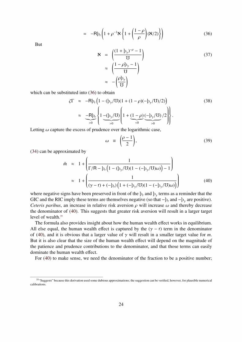
where negative signs have been preserved in front of the þr and þγ terms as a reminder that theGIC and the RIC imply these terms are themselves negative (so that −þr and −þγ are positive).Ceteris paribus, an increase in relative risk aversion ρ will increase ω and thereby decreasethe denominator of (40). This suggests that greater risk aversion will result in a larger targetlevel of wealth.35

The formula also provides insight about how the human wealth effect works in equilibrium.All else equal, the human wealth effect is captured by the (γ − r) term in the denominatorof (40), and it is obvious that a larger value of γ will result in a smaller target value for m.But it is also clear that the size of the human wealth effect will depend on the magnitude ofthe patience and prudence contributions to the denominator, and that those terms can easilydominate the human wealth effect.

For (40) to make sense, we need the denominator of the fraction to be a positive number;

35“Suggests” because this derivation used some dubious approximations; the suggestion can be verified, however, for plausible numericalcalibrations.

24

defining

þγ ≡ þγ(1 − (−þγ/f)ω), (41)

this means that we need:

(γ − r) > þr − þrþγ/f

=(ρ−1(r − ϑ) − r

)− þrþγ/f

γ > ρ−1(r − ϑ) − þrþγ/f

0 > ρ−1(r − ϑ) − γ︸ ︷︷ ︸þγ

−þr(þγ/f)

0 > þγ − þr(þγ/f). (42)

But since the RIC guarantees þr < 0 and the GIC guarantees þγ < 0 (which, in turn, guaranteesþγ < 0), this condition must hold.36

The same set of derivations imply that we can replace the denominator in (40) with thenegative of the RHS of (42), yielding a more compact expression for the target level ofresources,

m ≈ 1 +

1

þr(þγ/f) − þγ

= 1 +

( 1/(−þγ)1 + (−þr/f)(1 + (−þγ/f)ω)

). (43)

This formula makes plain the fact that an increase in either form of impatience, by increasingthe denominator of the fraction in (43), will reduce the target level of assets.

We are now in position to discuss (40), understanding that the impatience conditions guar-antee that its numerator is a positive number.

Two specializations of the formula are particularly useful. The first is the case where ρ = 1(logarithmic utility). In this case,

þr = −ϑ

þγ = r − ϑ − γω = 0

and the approximation becomes

m ≈ 1 +

(1

(γ − r) + ϑ(1 + (γ + ϑ − r)/f)

)(44)

which neatly captures the effect of an increase in human wealth (via either increased γ orreduced r), the effect of increased impatience ϑ, or the effect of a reduction in unemploymentrisk f in reducing target wealth.

36In more detail: For the second-order Taylor approximation in (36), we implicitly assume that the absolute value of the second-orderterm is much smaller than that of the first-order one, i.e. |ρ−1ℵ| ≥ |(ρ−1)(ρ−1 − 1)(ℵ2/2)|. Substituting (37), the above could be simplified to1 ≥ (−þγ/f)ω, therefore we have þγ < 0. This simple justification is based on the proof above that RIC and GIC guarantee the denominatorof the fraction in (34) is positive.

25

The other useful case to consider is where r = ϑ but ρ > 1. In this case,

þr = −ϑ

þγ = −γ

þγ = −γ(1 − (γ/f)ω)

so that

m ≈ 1 +

(1

(γ − r) + ϑ(1 + (γ/f)(1 − (γ/f)ω))

)(45)

where the additional term involving ω in this equation captures the fact that an increase in theprudence term ω shrinks the denominator and thereby boosts the target level of wealth.37

37It would be inappropriate to use the equation to consider the effect of an increase in r because the equation was derived under theassumption ϑ = r so r is not free to vary.

26

27

ReferencesAiyagari, S. Rao (1994): “Uninsured Idiosyncratic Risk and Aggregate Saving,” Quarterly

Journal of Economics, 109, 659–684.

Barsky, Robert B., F. Thomas Juster, Miles S. Kimball, and Matthew D. Shapiro (1997):“Preference Parameters and Behavioral Heterogeneity: An Experimental Approach in theHealth and Retirement Survey,” Quarterly Journal of Economics, CXII(2), 537–580.

Berk, Jonathan, Richard Stanton, and Josef Zechner (2009): “Human Capital, Bankruptcy,and Capital Structure,” Manuscript, Hass School of Business, Berkeley.

Bernanke, Benjamin, Mark Gertler, and Simon Gilchrist (1996): “The FinancialAccellerator and the Flight to Quality,” Review of Economics and Statistics, 78, 1–15.

Bewley, Truman (1977): “The Permanent Income Hypothesis: A Theoretical Formulation,”Journal of Economic Theory, 16, 252–292.

Cagetti, Marco (2003): “Wealth Accumulation Over the Life Cycle and PrecautionarySavings,” Journal of Business and Economic Statistics, 21(3), 339–353.

Carroll, Christopher D. (1992): “The Buffer-Stock Theory of Saving: SomeMacroeconomic Evidence,” Brookings Papers on Economic Activity, 1992(2), 61–156,Available at http://econ.jhu.edu/people/ccarroll/BufferStockBPEA.pdf.

(2001): “Death to the Log-Linearized Consumption Euler Equation! (And Very PoorHealth to the Second-Order Approximation),” Advances in Macroeconomics, 1(1), Article6, Available at http://econ.jhu.edu/people/ccarroll/death.pdf.

(2011): “Theoretical Foundations of Buffer Stock Saving,” Manuscript,Department of Economics, Johns Hopkins University, Latest version available athttp://econ.jhu.edu/people/ccarroll/papers/BufferStockTheory.pdf.

Carroll, Christopher D., and Olivier Jeanne (2009): “A Tractable Model of PrecautionaryReserves, Net Foreign Assets, or Sovereign Wealth Funds,” NBER Working Paper Number15228.

Carroll, Christopher D., and Miles S. Kimball (1996): “On the Concavity ofthe Consumption Function,” Econometrica, 64(4), 981–992, available at http://econ.jhu.edu/people/ccarroll/concavity.pdf.

Chamberlain, Gary, and Charles A. Wilson (2000): “Optimal Intertemporal ConsumptionUnder Uncertainty,” Review of Economic Dynamics, 3(3), 365–395.

Clarida, Richard H. (1987): “Consumption, Liquidity Constraints, and Asset Accumulationin the Face of Random Fluctuations in Income,” International Economic Review, XXVIII,339–351.

28

Fisher, Irving (1930): The Theory of Interest. MacMillan, New York.

Friedman, Milton A. (1957): A Theory of the Consumption Function. Princeton UniversityPress.

Gourinchas, Pierre-Olivier, and Jonathan Parker (2002): “Consumption Over the LifeCycle,” Econometrica, 70(1), 47–89.

Hall, Robert E. (1988): “Intertemporal Substitution in Consumption,”Journal of Political Economy, XCVI, 339–357, Available athttp://www.stanford.edu/~rehall/Intertemporal-JPE-April-1988.pdf.

Jagannathan, Ravi, Keiichi Kubota, and Hitoshi Takehara (1998): “Relationship betweenLabor-Income Risk and Average Return: Empirical Evidence from the Japanese StockMarket,” Journal of Business, 71(3), 319–47.

Kimball, Miles S. (1990): “Precautionary Saving in the Small and in the Large,”Econometrica, 58, 53–73.

Krusell, Per, and Anthony A. Smith (1998): “Income and Wealth Heterogeneity in theMacroeconomy,” Journal of Political Economy, 106(5), 867–896.

Markowitz, Harold (1959): Portfolio Selection: Efficient Diversification of Investment. JohnWiley & Sons, New York.

Merton, Robert C. (1969): “Lifetime Portfolio Selection under Uncertainty: The ContinuousTime Case,” Review of Economics and Statistics, 50, 247–257.

Parker, Jonathan A., and Bruce Preston (2005): “Precautionary Saving and ConsumptionFluctuations,” American Economic Review, 95(4), 1119–1143.

Phelps, Edward S. (1960): “The Accumulation of Risky Capital: A Sequential UtilityAnalysis,” Econometrica, 30(4), 729–743.

Samuelson, Paul A. (1969): “Lifetime Portfolio Selection by Dynamic StochasticProgramming,” Review of Economics and Statistics, 51, 239–46.

Schechtman, Jack, and Vera Escudero (1977): “Some results on ‘An Income FluctuationProblem’,” Journal of Economic Theory, 16, 151–166.

Sethi, S.P., andG.L. Thompson (2000): Optimal Control Theory: Applications to ManagementScience and Economics. Kluwer Academic Publishers, Boston.

Tobin, James (1958): “Liquidity Preference as Behavior Towards Risk,” Review of EconomicStudies, XXXV(67), 65–86.

Toche, Patrick (2005): “A Tractable Model of Precautionary Saving inContinuous Time,” Economics Letters, 87(2), 267–272, Available athttp://ideas.repec.org/a/eee/ecolet/v87y2005i2p267-272.html.

29

Zeldes, Stephen P. (1989): “Optimal Consumption with Stochastic Income: Deviations fromCertainty Equivalence,” Quarterly Journal of Economics, 104(2), 275–298.

30