A TOOL FOR OLAP (ON-LINE ANALYTICAL

PROCESSING) ON TEXT DOCUMENTS

by

Ling-Chih Yvonne Cheng B.Sc., Simon Fraser University, 2006

PROJECT SUBMITTED IN PARTIAL FULFILLMENT OF THE REQUIREMENTS FOR THE DEGREE OF

MASTER OF SCIENCE

in the School of Computing Science Faculty of Applied Sciences

© Ling-Chih Yvonne Cheng 2011

SIMON FRASER UNIVERSITY

Summer 2011

All rights reserved. However, in accordance with the Copyright Act of Canada, this work may be reproduced, without authorization, under the conditions for Fair Dealing. Therefore, limited reproduction of this work for the purposes of private

study, research, criticism, review and news reporting is likely to be in accordance with the law, particularly if cited appropriately.

ii

APPROVAL

Name: Ling-Chih Yvonne Cheng

Degree: Master of Science

Title of Project: A tool for OLAP (On-Line Analytical Processing) on text documents

Examining Committee:

Chair: Fred Popowich

______________________________________

Jian Pei Senior Supervisor

______________________________________

Ke Wang Supervisor

______________________________________

Wo-Shun Luk [Internal] Examiner

Date Defended/Approved: August 8, 2011

Last revision: Spring 09

Declaration of Partial Copyright Licence

The author, whose copyright is declared on the title page of this work, has granted to Simon Fraser University the right to lend this thesis, project or extended essay to users of the Simon Fraser University Library, and to make partial or single copies only for such users or in response to a request from the library of any other university, or other educational institution, on its own behalf or for one of its users.

The author has further granted permission to Simon Fraser University to keep or make a digital copy for use in its circulating collection (currently available to the public at the “Institutional Repository” link of the SFU Library website <www.lib.sfu.ca> at: <http://ir.lib.sfu.ca/handle/1892/112>) and, without changing the content, to translate the thesis/project or extended essays, if technically possible, to any medium or format for the purpose of preservation of the digital work.

The author has further agreed that permission for multiple copying of this work for scholarly purposes may be granted by either the author or the Dean of Graduate Studies.

It is understood that copying or publication of this work for financial gain shall not be allowed without the author’s written permission.

Permission for public performance, or limited permission for private scholarly use, of any multimedia materials forming part of this work, may have been granted by the author. This information may be found on the separately catalogued multimedia material and in the signed Partial Copyright Licence.

While licensing SFU to permit the above uses, the author retains copyright in the thesis, project or extended essays, including the right to change the work for subsequent purposes, including editing and publishing the work in whole or in part, and licensing other parties, as the author may desire.

The original Partial Copyright Licence attesting to these terms, and signed by this author, may be found in the original bound copy of this work, retained in the Simon Fraser University Archive.

Simon Fraser University Library Burnaby, BC, Canada

iii

ABSTRACT

We want to automate the process of summarizing a collection of

documents, and get an overall picture of the topics covered by the document

collection. The summarized results should be easy to understand with simple

visualization and able to get more details on selected topics by performing

various operations. The purpose is to help users to save time on finding out

interesting articles, and focus only on useful articles and conduct further analysis

as they desire.

In order to achieve this goal, we developed the tool Docs Summarizer,

where we introduced Online Analytical Processing (OLAP) into document set

summarization. Our Tool can take a collection of documents as input, and apply

analysis on them to generate a series of meaningful outputs. The outputs include

a list of top k analysis level categories and a two-dimensional matrix chart. The

users can do further exploration on the outputs by performing various operations.

Keywords: tool; Online Analytical Processing; summarizing documents; visualization results

iv

ACKNOWLEDGEMENTS

I would like to express my gratitude to all those who gave me the

encouragement to complete this project.

Especially, I am deeply indebted to my senior supervisor Dr. Jian Pei for

all the valuable comments and supports during the entire research &

development period of my project. I would like to express my appreciation to Jian

for his time and patience.

I also want to thank Prof. Ke Wang, Wo-Shun Luk, and Fred Popowich for

the insightful discussions during the oral defence exam.

v

TABLE OF CONTENTS

Approval .......................................................................................................................... ii

Abstract .......................................................................................................................... iii

Acknowledgements ........................................................................................................ iv

Table of Contents ............................................................................................................ v

List of Figures................................................................................................................ vii

1: Introduction ............................................................................................................... 1

1.1 Motivation................................................................................................................ 1

1.2 Objectives ............................................................................................................... 2

1.3 Related Work .......................................................................................................... 3

1.4 Organization of the Report ...................................................................................... 6

2: Specification .............................................................................................................. 7

2.1 Terminology ............................................................................................................ 7

2.2 Project Description ................................................................................................ 10

2.3 Assumptions ......................................................................................................... 12

2.4 Application Interface .............................................................................................. 13

2.5 Application Operations .......................................................................................... 16

2.5.1 Redraw Matrix Chart .................................................................................. 16 2.5.2 View Article ................................................................................................ 17 2.5.3 Operations on Cells of the Matrix Chart ..................................................... 17 2.5.4 Operations on Sub-Row and Sub-Column of the Matrix Chart ................... 18 2.5.5 View Category Sub Tree ............................................................................ 19

3: Algorithms ............................................................................................................... 21

3.1 A Baseline Approach ............................................................................................. 21

3.1.1 Tool Structure ............................................................................................ 21 3.1.2 Algorithm Overview and Framework .......................................................... 22 3.1.3 Pre-Processing .......................................................................................... 25 3.1.4 Generating Top K Categories .................................................................... 29 3.1.5 Generating Result Charts .......................................................................... 34

3.2 Operations in Detail ............................................................................................... 38

3.2.1 Redraw Matrix Chart .................................................................................. 38 3.2.2 View Article ................................................................................................ 39 3.2.3 Rank Article on the Selected Cell of the Matrix Chart ................................. 39 3.2.4 Drilling Operation on the Selected Cell of the Matrix Chart ........................ 39 3.2.5 Operations on Sub-Row and Sub-Column of the Matrix Chart ................... 40 3.2.6 View Category Sub Tree ............................................................................ 41

3.3 Bottlenecks and Improvements for the Baseline Solution ...................................... 41

3.3.1 Improving Pre-Processing ......................................................................... 42

vi

3.3.2 Improving Top K Category Generation ...................................................... 44 3.3.3 Improving Result Charts Generation .......................................................... 46

4: Empirical Evaluation ............................................................................................... 49

4.1 Dataset and Pre-processing .................................................................................. 49

4.2 Case Study: Avoid the Least Popular Restaurants in Town ................................... 50

5: Conclusions and Future Work ............................................................................... 59

5.1 Summary of the Project ......................................................................................... 59

5.2 Future Work .......................................................................................................... 60

Reference List ............................................................................................................. 61

vii

LIST OF FIGURES

Figure 1 Example of a Matrix Chart and the Related Terminologies ................................ 7

Figure 2 Example of a Category Tree .............................................................................. 9

Figure 3 General Flow of using Docs Summarizer ........................................................ 11

Figure 4 Docs Summarizer Interface ............................................................................. 13

Figure 5 Enlarged Screen Shot of Result Frame ........................................................... 14

Figure 6 Enlarged Screen Shot of a Matrix Chart .......................................................... 14

Figure 7 List of Available Cells and Available Operations .............................................. 17

Figure 8 Operations on Sub-Row and Sub-Column ....................................................... 18

Figure 9 Category Sub Tree Chart ................................................................................ 19

Figure 10 Docs Summarizer Components and Their Interactions .................................. 21

Figure 11 Flow of the Three Stages in Baseline Algorithm ............................................ 22

Figure 12 Screen out Quality Words for Input Document Collection .............................. 25

Figure 13 A Category Hierarchy Example from WordNet .............................................. 26

Figure 14 Structure of a Category Tree with Sorted Index ............................................. 27

Figure 15 A Concrete Example of a Category Tree with Sorted Index ........................... 28

Figure 16 Look up Analysis Level Categories and Sub-Categories for All Quality Words ........................................................................................................... 30

Figure 17 An Example of Selected Analysis Level Categories and Sub-Categories .................................................................................................... 31

Figure 18 Category Information of Category A and Category B ..................................... 34

Figure 19 Process to Apply Cross Products .................................................................. 35

Figure 20 Example of Matrix Cell Information ................................................................ 36

Figure 21 Example of a Matrix Chart ............................................................................. 37

Figure 22 Analysis Results for Using the Restaurant Review Dataset as Input .............. 50

Figure 23 Matrix Chart for Users-Selected Categories .................................................. 51

Figure 24 Part of the Enlarged Matrix Chart for Users-Selected Categories .................. 52

Figure 25 New Analysis Results for Documents Related to "Wrong doing, wrongful conduct, misconduct" And "Course" ................................................ 53

viii

Figure 26 New Analysis Results of "Hash out, discuss, talk over" and "Wait, waitress" Categories for Documents Related to "Wrong doing, wrongful conduct, misconduct" And "Course" .............................................................. 54

Figure 27 New Matrix Chart of "Hash out, discuss, talk over" and "Wait, waitress" Categories for Documents Related to "Wrong doing, wrongful conduct, misconduct" And "Course" ............................................................................ 54

Figure 28 Chosen Article: “Alta – Spanish.txt” ............................................................... 55

Figure 29 Related Comments from the Chosen Article: “Alta – Spanish.txt” .................. 56

Figure 30 List of Ranked Articles for Cell with Value Pair of “Tip off, tip” And “Wait, Waitress” ............................................................................................ 57

Figure 31 Some Example of Articles ............................................................................. 57

1

1: INTRODUCTION

1.1 Motivation

Travis is planning a trip for his two-week vacation, but he cannot decide

where to go. He browses through several of his favourite blogs and tries to find

articles related to interesting travel experiences. However, it is painful to go

through each post and there is no guarantee when and where he can find what

suits him. He is thinking that it would be great if there were a tool for him to input

links of different blogs, and generate a summary for all posts automatically. The

summary can be a list of categories ranked by its importance, so that he can pick

some categories he is interested in and read more related posts.

Victor is the manager of a sales department. He asks each of his

employees to collect feedbacks of their newest product, but ends up with a large

number of text documents that contain customer/user reviews from different

sources. He is now having a headache to sort out and to summarize all the

opinions they gathered. It is time consuming if he reads each review one by one,

and he wants to see the big picture of the overall feedback. It is hard to do the

task manually. Victor thinks he should use some tools to automate the task. He

would like to use the tool to analyze all review documents and get a list of ranked

aspects from the review collection. Based on the given list of ranked aspects, he

could conduct further analysis on the categories that need more attentions from

him. It will be more efficient and effective than conducting the task manually.

2

To conclude, we see that there is a strong need for a text summarization

tool, which can summarize a collection of text documents and help users to save

time on finding out interesting articles. By using the tool, users can focus on

useful articles only and conduct further analysis as they desire. Therefore, we

developed the tool Docs Summarizer to achieve this goal.

1.2 Objectives

We want to automate the process of summarizing a collection of

documents, and get an overall picture of the topics covered by the document

collection. The summarized results should be easy to understand with simple

visualization. In addition, users should be able to get more details on selected

topics.

To achieve our goal, we introduced Online Analytical Processing (OLAP)

into document set summarization (Chaudhuri & Dayal, 1997). OLAP is a category

of applications that collects, processes and presents multidimensional data for

decision support. OLAP applications allow users to conduct further explorations

on data by providing functionalities such as drilling down and drilling up. The

output of an OLAP application often displays in a matrix format. The dimensions

form the rows and columns of the matrix, and the measures form the values of

the matrix (Mailvaganam, 2007).

In our project, our tool Docs Summarizer performs the tasks described

above by applying an OLAP solution to summarize a given collection of

documents. Our solution has the following features:

3

The summarized results are lists of categories, which cover the given

collection of documents

A list of categories is ranked by its importance

A matrix chart, which provides further details for two selected

categories, is presented to users.

Users can explore more details by drilling down on selected

categories.

1.3 Related Work

There are many researches conducted on the field of text summarization

in the last half century. They can be roughly grouped into single-document

summarization and multi-document summarization. We briefly introduce each

area in this section.

There are two major methodologies proposed for the early work of single-

document summarization. The first methodology emphasizes the frequencies of

non-stop words, and those frequencies are treated as useful measures of word

significance (Luhn, 1958). The second methodology proposed that sentence

position indicates the relatively importance of each sentence; therefore, we can

find out the possible topic sentence for an article (Baxendale, 1958). In recent

decades, Natural Language Processing (NLP) becomes the mainstream

approach for text summarization. Some major works include Naive-Bayes

method with independence assumption (Kupiec, Pedersen & Chen, 1995) and

some learning algorithm with no independence assumption, such as hidden

4

Markov model (Conroy & O'Leary, 2001), log-linear models (Osborne, 2002), and

neural networks (Svore, Vanderwende & Burges, 2007).

The other area for text summarization is the multi-document

summarization, where the main goal is to extract a single summary from multiple

documents. SUMMONS is one of the summarization system developed by the

NLP group at Columbia University (Mckeown & Radev, 1995). It is a template-

driven system and is designed to work on a strict, narrow domain. The system

tends to be problematic when it works on a generalized, broader domain.

However, the issue was addressed and improved in later years by McKeown et

al (McKeown, Klavans, Hatzivassiloglou, Barzilay & Eskin, 1999). The improved

system employ techniques such as evaluating single words by their TD-IDF

weighted scores and using single words synsets information from WordNet

(Miller, 1995).

The other major application for multi-document summarization is MEAD,

and MEAD is a large-scale system that aimed to work on general domains

(Radev et al., 2004). Each document in MEAD is represented as a bag of words,

and there are two stages to perform in the system. The first stage is topic

detection, which groups articles describing the same event together. The second

stage is to identify central sentences in each group, and the central sentence are

outputted as the summarized results. We can see the two summarization

systems distinguish themselves by aiming at different ranges of domain, and the

summarized results from both systems are in paragraph style.

5

One of the other major categories for multi-document summarization is the

topic-driven summarization. Topic-driven feature implies a dependency on

queries, and different queries may lead to different summarization results. The

reasoning behind is that different users with different information needs may

require different summary of the same document (Carbonell & Goldstein, 1998).

The main representations include Maximal Marginal Relevance (MMR)

(Carbonell & Goldstein, 1998) and Graph Spreading Activation (Mani & Bloedorn,

1997).

Maximal Marginal Relevance treats each sentence or paragraph as a

token and calculates a score by reward relevant sentences and punish redundant

ones (Carbonell & Goldstein, 1998). The tokens with the highest score are

presenting as the summary results. Graph Spreading Activation finds similarities

and dissimilarities between pairs of documents using a graph-based method

(Mani & Bloedorn, 1997). Each document is represented by a graph using nodes

and edges, and the common nodes and different nodes between a pair of

document graph are identified. The sentences with highest common score and

highest different scores are output as the summarization results.

Our tool aims to perform multi-document summarization, and it

differentiates itself by conducting keywords summarization instead of paragraph-

style or headline-style summarization. In addition, we employ the TF-IDF

technique, as it is consistent with language model in theory. However, we apply

TF-IDF on the category of a single word instead of the single word itself. The

argument is that, comparing to a frequent single word, a frequent category is a

6

better representation of a document. The category hierarchy information is

extracted from the external tool WordNet (Miller, 1995).

1.4 Organization of the Report

The rest of our report has four major sections. The next section contains

detailed project description and major project screen shots for illustration. In

Section 3, we first demonstrate our baseline solution and identify some potential

problems associated with this solution, then introduce an improved version of

solution to conquer some of the issues we encountered. Section 4 provides one

interesting empirical use case studies by applying our solution on a real dataset.

Finally, Section 5 concludes our project and lists possible future work to enhance

project results.

7

2: SPECIFICATION

In this chapter, we first introduce important terminologies that will be used

throughout the report. Then, we present a detailed project description and major

project screen shots for illustration. The main operations for our tool, Docs

Summarizer, are also discussed in this chapter.

2.1 Terminology

Before we describe our tool in more details, we will introduce several

terminologies which will be used throughout the report.

Figure 1 Example of a Matrix Chart and the Related Terminologies

Matrix chart: A chart that summarizes a multidimensional dataset into

a grid. Please refer to Figure 1 for an example of a matrix chart.

8

Row: The vertical header of a matrix chart. Refer to the matrix chart in

Figure 1, the row is in dark blue background color and the value of the

row is “organism, being”.

Sub-Row: The secondary vertical header of a matrix chart. Refer to

the matrix chart in Figure 1, the sub-row is in light blue background,

and there are two values for the sub-rows, which are “animal, animate-

being, beast, brute, creature, fauna” and “person, individual, someone,

somebody, mortal, soul”.

Column: The horizontal header of a matrix chart. Refer to the matrix

chart in Figure 1, the column has a dark blue background color, and

the value of the column is “activity”.

Sub-Column: The secondary horizontal header of a matrix chart.

Refer to the matrix chart in Figure 1, the sub-column is in light blue

background color, and there are three sub-column values, which are

“diversion, recreation”, “representation”, and “sensory activity”.

Cell: The grid of a matrix chart. We refer each cell by its sub-row and

sub-column value pair. For example, we refer the cell at the left top

corner in Figure 1 as pair (“animal, animate-being, beast, brute,

creature, fauna”, “diversion, recreation”). Also, each cell in a matrix

chart has a value. For example, the cell at the left top corner of the

matrix chart in Figure 1 has value “3x1.3”.

9

Figure 2 Example of a Category Tree

Category Tree: A tree with a hierarchy of category. The root of the

category tree is the most general category, comparing to its entire

descendant. Each node in the tree must be a sub-category of its

parent, and all of its children must be sub-categories of the node. We

can see an example of a category tree in Figure 2. Note that the

category tree grows from left to right instead of top to bottom. The root

node, which is category “entity”, is circled by a blue border and is the

parent/ancestor category of all other categories in the tree. The internal

nodes, which are surrounded by gray borders, are sub-categories of

their parents. Each internal node is also the parent/ancestor category

for all of its children/descendants. The leaf nodes with orange borders

are the most specific categories. Each of the leaf nodes is a sub-

category of its parents, but has no sub-categories as children.

10

Category Level: The level of nodes in a category tree. Category level

is numbered in sequence starting from the tree root, and therefore the

root has category level 1. The category level number of a node is the

length of the path from the root to the node. The category level is

increased by 1 when the length of the path is increased by 1. Refer to

Figure 2, we see there are 3 nodes belonging to category Level 2:

“abstraction, abstract entity”, “organism, being”, and “thing”. The

deepest category level for the category tree in Figure 2 is Level 6, with

only one node at this level.

Analysis Level: The category level for the result category list

generated by our tool.

Category Sub Tree: A sub tree of the category tree. We can pick any

node in the category tree to be the root of the category sub tree. The

category sub tree contains all descendant nodes of the chosen root

node.

2.2 Project Description

We will develop Docs Summarizer, which can interactively explore a

collection of text documents and present users an overview of topics covered.

We will provide visualization results so that users can capture main topics at a

glance. Possible applications include blog reading tool, web page browsing tool,

opinion summarizing tool, etc. All of these tools provide summarized results of

11

Figure 3 General Flow of using Docs Summarizer

a collection of text documents and allow users to explore on interesting facets

intertactively.

To obtain an overall idea of the general flow of our tool, we can refer to

Figure 3. The main purpose of the tool is to identify the top k categories from a

given collection of documents, where k is an input parameter provided by users.

Users can select two categories from the top k categories as the matrix chart row

and column, and the tool will generate a 2D matrix chart as the visualization

result. By default, the top two ranked categories are used as row and column, but

users can select different categories and redraw the matrix chart. The sub-row

values and sub-column values are the corresponding sub-categories of row and

column categories. Each cell on the matrix chart represents documents covered

by the specific pair of the sub-row value and sub-column value.

There are several operations available for Docs Summarizer. The purpose

is to allow users to explore the result interactively. Users can increase the

category level of sub-row or sub-column, in order to explore how documents in

each cell scatter on a less general sub-row value or a less general sub-column

12

value. By choosing a certain cell on the matrix chart, further drill down analysis

can be applied to the documents associated with the cell. A new list of top k

categories and a new matrix chart will be generated. More details on operations

will be discussed in section 2.5.

2.3 Assumptions

For simplification, we assume that one file contains only one document,

and the input for this tool is the directory of the entire document collection, which

users would like to analyze.

To keep our discussion simple, we do not consider phrases consisting of

more than one word, such as “Stanley Park” or “Deer Lake”. We assume all

words are separated terms and do not consider their orders as well.

We have a strong dependency on how words in the document collection

are classified into categories, and how we build the category tree. For simplicity

and result consistency, we use the external tool WordNet (Miller, 1995) to assign

category to each word, and use it to build the category tree.

For the category tree we built for our tool, we further assume that there is

no cycle contained in the tree, and a word may be included in the tree several

times if it belongs to more than one category.

13

2.4 Application Interface

Figure 4 Docs Summarizer Interface

The Docs Summarizer interface consists of four frames: Upload Frame,

Setting Frame, Result Frame, and Article Frame. Please refer to Figure 4 to see

a real case example.

The Upload Frame allows users to load document collection by

providing the collection directory.

The Setting Frame allows users to adjust settings of analysis level and

the number of categories to be generated in the analyzed result.

The Result Frame shows the visualization result of the document

collection, and some control elements for users to interact with the

result. Please refer to Figure 5 for an enlarged screen shot of the

Result Frame.

14

Figure 5 Enlarged Screen Shot of Result Frame

The Article Frame displays document content selected by users. A

user can choose interesting document from the collection to read, and

the frame will only display one document at a time.

Figure 6 Enlarged Screen Shot of a Matrix Chart

One of the major results for our tool is the matrix chart in the Result Frame.

We use the enlarged matrix chart in Figure 6 for illustration, and we label three

cells as cell 1, cell 2, and cell 3 for the ease of reference. The column and row

values are selected categories, and the sub-column and sub-row values are sub-

15

categories associated with the column and row categories. For each cell, it has a

value in the form of “number of documents belonging to the cell x the average

count of the times that the sub-row value and sub-column value appear together

in each document”. For example, we see that the value for cell 1 is “3x1.3”, and

cell 1 has a sub-row value “animal, animate-being, beast, brute, creature, fauna”

and a sub-column value “diversion, recreation”. We can interpret the value of cell

1 as the following: “There are three documents that contain both the sub-

categories „animal, animate-being, beast, brute, creature, fauna‟ and „diversion,

recreation‟. Consider the two sub-categories as a pair. We count the number of

times that the sub-category pair occurs in each of the three documents. The

average count, which is total number of times that the sub-category pair occurs

divided by total number of documents, is 1.3”.

In the matrix chart, the border width of each cell reflects the number of

documents belonging to it, and the background colour of each cell reflects its

relative importance comparing to all other cells in the matrix chart. The thicker

the border means the larger number of documents, and the darker the

background colour means the greater importance of the cell. In order to become

more important, the sub-category pair of a cell needs to have a higher average

appearance rate in the associated documents. For example, in Figure 6, we see

that there are three documents containing the sub-category pair in cell 1, while

there is only one document containing the sub-category pair in cell 2. Therefore,

the border for cell 1 is thicker than cell 2. By looking at the average count of

times that the sub-category pair occurs, we see that cell 3 has a higher average

16

count than cell 1 and cell 2. Therefore, it has a darker background colour than

the other two cells.

2.5 Application Operations

There are several operations available for our tool, and we will describe

the function of each in the section. Here is a list of our five main operations:

Redraw matrix chart by selecting two categories from the top k

categories list.

View full article by selecting an article name.

For each cell of the matrix chart, we can rank articles according to

their contributions, drill down for further analysis, or drill back up.

For sub-row and sub-column of the matrix chart, we can increase

their category levels, or decrease their category levels back to the

initial level.

View category sub trees for the row category and column category of

the matrix chart.

2.5.1 Redraw Matrix Chart

Instead of using default categories, which is the top two ranked categories

among the top k categories list, the user can select any other two categories from

the top k categories list and generate a new matrix chart.

17

Figure 7 List of Available Cells and Available Operations

2.5.2 View Article

The titles of all articles from the input document collection are listed in a

dropdown menu. The users can choose any document title from the dropdown

menu to view the full document at the Article Frame below.

2.5.3 Operations on Cells of the Matrix Chart

We refer each cell by the pair of its sub-row value and sub-column value.

The value pair of each cell is listed in a dropdown menu. Refer to Figure 7, we

can see an example of value pair of a cell as “animal, animate-being, beast,

brute, creature, fauna” and “turn, play”. Other possible value pair of a cell can be

“person, individual, someone, somebody, mortal, soul” and “occupation,

business, job, line of work, line”.

After selecting a cell, there are three types of operations to perform. We

can rank articles belonging to the cell according to their contributions. The

contribution is the count of times that the cell value pair appears in one

document. For the chosen cell in Figure 7, the value pair appears in document

“Memory.txt” two times, which has a higher appearance frequency comparing to

the other two documents. Therefore, it is ranked as the top contributor to the

chosen cell.

18

Figure 8 Operations on Sub-Row and Sub-Column

We can also drill down on a cell for further analysis. When we perform

drilling down analysis on a chosen cell, our tool will reflect the change by

regenerating the list of top k categories and a new matrix chart in the Result

Frame. Finally, we can drill the cell up until it is back to its initial level. Refer to

Figure 7, the “Drill Down” button will grey out after we perform drilling down on a

single document, since further drill down operation does not make sense on a

single document. For a similar reason, the “Drill Up” button will grey out when the

cell is drilled up to its initial level.

2.5.4 Operations on Sub-Row and Sub-Column of the Matrix Chart

There are two operations to perform on each sub-row and sub-column of

the matrix chart. We can increase the category levels of the sub-row and/or sub-

column to see how documents scatter on less general sub-categories. We can

also decrease the category levels until they are at their initial levels. Refer to

Figure 8, users can adjust the category levels by clicking the enabled buttons.

The “Lvl Down” buttons will grey out when the current sub-category level is the

least general sub-categories level, and the “Lvl Up” buttons will grey out when

the current sub-category level is same as its initial sub-category level.

19

Figure 9 Category Sub Tree Chart

2.5.5 View Category Sub Tree

In order to give users an overall idea on the row and column category

hierarchy, we provide one category sub tree chart for each. We can refer to

Figure 9 for an example of category sub tree chart. The root of the row category

sub tree is the row category, and the root of the column category sub tree is the

column category. Refer to the example in Figure 9, the category “organism,

being” has two sub-categories, which are “animal, animate-being, beast, brute,

creature, fauna” and “person, individual, someone, somebody, mortal, soul”. For

the sub-category “animal, animate-being, beast, brute, creature, fauna”, it has

three children with less general sub-categories: “Chordate”, “invertebrate”, and

“young, offspring”. Note that only the categories applicable to our document

collection are part of the category trees, and the current levels of sub-categories

for sub-row and sub-column are highlighted in yellow. Users can select to view

20

category sub tree for row or column category by switching the tab at the top of

the chart.

21

3: ALGORITHMS

In this chapter, we demonstrate our baseline solution and identify some

potential problems associated with this solution. We then introduce an improved

version of solution to conquer some of the issues we encountered.

3.1 A Baseline Approach

We propose a baseline solution for our tool in this section. First, we

illustrate our tool structure and introduce the overview of our algorithm. Then, we

break down the algorithm into several detailed steps and discuss each of them in

depth.

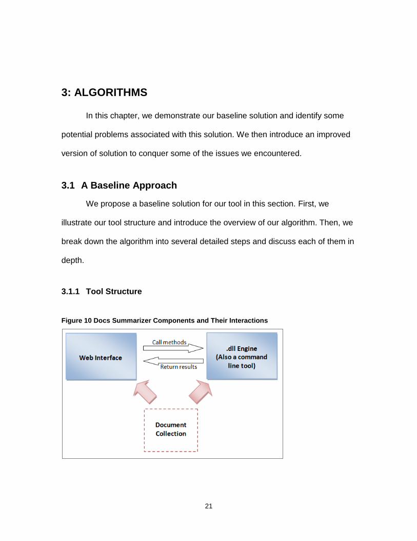
3.1.1 Tool Structure

Figure 10 Docs Summarizer Components and Their Interactions

22

There are two components for Docs Summarizer. One is the front-end

interface while the other one is the back-end engine. Refer to Figure 10, the

front-end component is the web interface which allows users to interact with our

tool. The back-end component is the dynamic-link library (dll) engine, which

provides all necessary functions to perform tasks in our tool. Note the engine

component is also a command line tool itself.

We can also refer to Figure 10 for interactions between the two

components. Both of them have access to the input document collection directly.

The web interface component sends all requests to the engine component, and

the engine component respond with the result data.

3.1.2 Algorithm Overview and Framework

Figure 11 Flow of the Three Stages in Baseline Algorithm

The main purpose of the algorithm is to identify the top k categories in the

analysis level from a given collection of documents, where k and analysis level

23

are inputs from users. Then, we will use the top k categories to generate

visualization results for user interaction. In order to achieve this goal, we divided

the task into three stages: the Pre-Processing Stage, the Analysis Stage, and the

Chart Generation Stage. We can refer to Figure 11 for the stage flow, and the

detailed steps for each stage are listed at the end of this section.

At the Pre-Processing Stage, our tool read in the input document

collection. For each document in the collection, we treat it as a bag of words. For

each word, we convert it to its original form. As an example, “teach” is the original

form for words “taught” and “teaches”. After we convert each word to its original

form, the second step is to screen out the quality words, which are all nouns and

all verbs.

Next, we use the external tool WordNet to build up a category tree on top

of the collection of quality words and assign category level to each node. Each

quality word is a leaf node in the category tree, and we use WordNet to look up

the category hierarchy for each quality word and build the category tree

accordingly. Note that sometimes a quality word might belong to more than one

category. In this case, we include all of its categories instead of trying to analyze

the document context.

After we built up the category tree for all quality words from the document

collection, we progress to the Analysis Stage. We assign score to each category

in the analysis level of the quality words, and then we aggregate scores for all

categories in the analysis level and rank them in descending order based on a

formula of the aggregated scores and documents coverage.

24

Finally, at the Chart Generation Stage, we generate a result ranking of top

k categories in the analysis level where k and analysis level are inputs from

users. Given the top k categories, our tool generates a matrix chart using the top

two ranked categories. Users can explore the results interactively by conducting

operations introduced in chapter 2.5.

Each of the three stages in Figure 11 can further divide into several steps,

which are listed below. More details are provided in following sections.

Stage 1: the Pre-Processing Stage

Step1: Upload the document collection

Step2: For the input document collection, screen out all quality words,

which are nouns and verbs in their original form. The result for each

document is saved as a bag of quality words.

Step 3: Build a category tree on top of all quality words and assign

category level to each node. We use WordNet as the reference tool to

look up category hierarchy for each quality word.

Stage 2: the Analysis Stage

Step 4: Look up the analysis level categories for all quality words in the

input document collection.

Step 5: Calculate ntf-idf score for the analysis level categories of all

quality words in the input document collection.

Step 6: Generate top k analysis level categories based on a formula of

aggregated analysis level category ntf-idf score and documents coverage

25

Stage 3: the Chart Generation Stage

Step 7: Generate information associated with the two selected categories

in order to produce the result matrix chart

Step 8: Generate the result matrix chart

3.1.3 Pre-Processing

Step1: Upload the document collection

Upload the input collection of documents into memory for later analysis.

Step2: For the input document collection, screen out all quality

words, which are nouns and verbs in their original form. The result for each

document is saved as a bag of quality words.

For each input document, we select only nouns and verbs and convert

each of them to its original form. We use the external tool WordNet to determine

the part of speech for each word, and convert recognized nouns and verbs to

their original form.

Figure 12 Screen out Quality Words for Input Document Collection

26

Then, each document is represented as a bag of quality words, which

implies that the order of quality words is not important. We can refer to Figure 12

to illustrate this step.

In addition to producing the representation of each document in the input

collection, we also generate a list of unique quality words appeared in the

document collection.

Step 3: Build a category tree on top of all quality words and assign

category level to each node. We use WordNet as the reference tool to look

up category hierarchy for each quality word.

For each quality word, we need to identify its category hierarchy from the

least general level to the most general level. The process is repeated on all

unique quality words in the input document collection, and WordNet is the tool we

employed to identify category hierarchy for each quality word.

Figure 13 A Category Hierarchy Example from WordNet

We can refer to Figure 13 to see an example we exacted from Wordnet.

For the quality word “bread”, it has a parent category “backed goods”, and a root

27

category “entity”. To see another example, the least general category for the

quality word “fire” is “nature event”, and the most general category for this quality

word is “entity”, which is a shared category tree root with the quality word

“bread”.

Figure 14 Structure of a Category Tree with Sorted Index

In order to look up the category hierarchy for any quality word in a more

efficient manner, we build a category tree on top of the list of unique quality

words in the input document collection. We can refer to Figure 14 to see the

category tree structure. Each quality word is a leaf node, and we can look up

more general categories by tracing up the tree. The tree root is the most general

category for all the quality words in the tree.

A quality word may belong to more than 1 category. If a quality word has n

parent categories, then n leaf nodes will be added into the tree. Each of the n leaf

node is linked by a sorted index for fast access. The sorted index contains all

unique quality words in the input document collection, and each quality word

associates with a linked list. Each node of the linked list points to the quality word

28

node in the category tree. The quality word, which belongs to a large number of

categories, has a longer linked list. We can refer to Figure 14 to see the structure

of the category tree with a sorted index.

Figure 15 A Concrete Example of a Category Tree with Sorted Index

We can refer to Figure 15 to see a concrete example. The quality word

“check” has two sets of definition; therefore, it has two sets of category hierarchy.

One path of the category hierarchy from the least general category to the most

general category is “check”, “order of payment”, “legal document”, and “entity”.

The other path is “check”, “proof”, and “entity”. In this example, we need to add

two leaf nodes with value “check” into the tree, and each of the category

hierarchy is represented by the branch path to the tree root. Then, we insert

quality word “check” to the sorted index table and create a linked list with two

nodes. Each of the node points to a different “check” leaf node in the tree. By

constructing the category tree with sorted index, we can look up quality words

and their hierarchy categories quickly and easily.

29

When we insert a node into the tree, a category level number is assigned

to it. The most general category level is “1”, and the next less general category

level is “2”. The category level is increased by 1 as we navigate one level down

in the tree. The assignment continues until we reach the tree leaf, which is the

quality word itself. We can refer to Figure 15 to see the category tree with

category level assigned for each node.

The purpose of assigning category level is to make sure we can compare

all quality words in the collection of documents at the same scale. For example, a

document may have both “apple” and “fruit” appeared. Without converting them

to the same category level, we will count “apple” once and “fruit” once. If we

convert both of them to the same category level, “food” as an example, then we

will have 2 counts for “food”. The analysis level, which is the category level to

perform analysis, is an input from the user.

3.1.4 Generating Top K Categories

Step 4: Look up the analysis level categories for all quality words in

the input document collection.

In each document, we loop through all quality words, which are

recognized nouns and verbs in their original forms. The purpose is to look up the

analysis level categories, as well as the analysis level sub-categories. The

analysis level sub-categories are the categories with their category level equal to

analysis level plus 1. The reason for tracking the analysis level sub-categories is

30

Figure 16 Look up Analysis Level Categories and Sub-Categories for All Quality Words

that we use them as sub-row and sub-column values in the result matrix chart.

We can refer to Figure 16 for an illustration. The red box in Figure 16 represents

the analysis level categories, while the purple box represents the analysis level

sub-categories.

If a quality word has more than one analysis level category, we include all

of them instead of trying to do content analysis. In addition, if the quality word

has its least general category level smaller than the analysis level, then we treat

the quality word as the analysis level sub-category, and treat its parent node as

analysis level category.

31

Figure 17 An Example of Selected Analysis Level Categories and Sub-Categories

We can refer to Figure 17 to see an example. Suppose we set the

analysis level to “3”, the analysis level categories in Figure 17 are in red colour,

and the analysis level sub-categories are in purple colour. Note that the least

general category level of the quality word located in the second branch of the

tree is “2”, which is smaller than the analysis level “3”. Therefore, we treat the

quality word located in the second branch as analysis level sub-category, and we

treat its parent as analysis level category.

Step 5: Calculate ntf-idf score for the analysis level categories of all

quality words in the input document collection.

We need to calculate the normalized tf-idf score for the analysis level

categories in each document. The analysis level is an input from users. Category

level 1 represents the most general category. As the category level increases,

the category becomes less general.

In order to calculate the normalized tf-idf, we need to calculate its

normalized term frequency (ntf) and Inverse Document Frequency (idf). The

reason to calculate a normalized term frequency instead of a pure term

32

frequency is to avoid favoring longer documents. To compute normalized term

frequency, we use the formula listed below, where t represents for “analysis level

category” and d represents for “docuement”.

ntft,d = a + (1 − a)tft,d

tfmax (d)

For each document d, let the maximum term frequency be the analysis

level category with the highest frequency count. To represent this in a math

formula, we have tfmax (d)=max(τ∈d) tf(τ,d) , where τ ranges over all analysis level

categories in d. For each analysis level category t in a document, we compute its

normalized term frequency and a is a smoothing factor which we set to 0.4 here.

ntft,d = 0.4 + 0.6 ×tft,d

tfmax (d)

After we compute the ntf for each quality word in all documents, the next

thing is to calculate the Inverse Document Frequency (idf). The purpose is to

measure its general importance of a certain analysis level category. The formula

to compute idf is listed below.

idft = log𝑁

dft + 1

In this formula, N is the total number of documents in the collection, and

dft is the document frequency for the analysis level category t. We define the

document frequency as the total number of documents in the collection which

contain the analysis level category. The reason to plus 1 on dft in the

denominator is to make a correction to the case when there is no document

33

contained a certain analysis level category t. We prevent the error caused by the

number of documents divided by zero.

Finally, we can compute the ntf-idf for each analysis level category in each

document using the previous results. We gain ntf-idf by using the normalized

term frequency and multiple it by the inverse document frequency. The higher

score for the ntf-idf means the higher normalized term frequency and the lower

document frequency. Thus, the analysis level category is more important. The

formula is listed below.

ntf − ifd = ntft,d × idft

Step 6: Generate top k analysis level categories based on a formula

of aggregated analysis level category ntf-idf score and documents

coverage

First, we need to aggregate the ntf-idf score for the analysis level

categories. For each analysis level category, we sum up the total ntf-idf score.

We get a list of unique categories, and each one is associated with its total ntf-idf

score. We refer the aggregated score for each category as category score.

We need to produce a set of k categories which satisfy two requirements.

First, each category in the set needs to be frequent. Next, each of the k-

categories needs to cover as many documents as possible. We will determine

the importance of a category using its category score and multiply it by the

number of documents being covered. The formula is listed below.

𝑖𝑚𝑝𝑜𝑟𝑡𝑎𝑛𝑐𝑒 = category score × number of documents covered

34

We start with an empty list and keep adding category which has the

highest importance score until we have k items in the list. The list is the resulting

top k analysis level categories.

3.1.5 Generating Result Charts

Step 7: Generate information associated with the two selected

categories in order to produce the result matrix chart

Given the top k analysis level categories, users can select two of them to

generate the matrix chart. Otherwise, by default, the top-ranked category is used

as the row value and the second-ranked category is used as the column value for

the matrix chart. For each of the two selected categories, we need to trace three

things: the documents that contained the category, the associated sub-categories

in the documents that contained the category, and the appearance frequency for

the associated sub-categories in the documents that contained the category.

Figure 18 Category Information of Category A and Category B

We can refer to Figure 18 to see an illustration. Suppose the two selected

categories are A and B, we need to track the documents contained them. In

35

Figure 18, we see category A are contained by document 1, 2, and 3 while

category B are contained by document 1, 3, and 4. For each document, we also

track the sub-categories that appeared in it, and the associated frequencies.

Refer to Figure 18, we see there are 3 sub-categories for category A in document

1, which are sub-category A-1, A-2, and A-3. The number of times that A-1

appeared in document 1 is “1”, and the number of times for A-2 appeared in

document 1 is “2”. We refer all information associated with each category as

category information.

The purpose to produce category information for each category is to

determine which sub-categories to be included in the matrix chart. Not every sub-

category will show on the matrix chart. Only the sub-categories from the

documents that contain both selected categories are included in the matrix chart.

To illustrate by an example from Figure 18, only the sub-categories appeared in

document 1 and document 3 are included in the matrix chart, since they are the

only two documents that contain both category A and category B.

Figure 19 Process to Apply Cross Products

36

After we generate category information, we can produce the information

required for the matrix cells. For each document that contains both selected

categories, we do cross products on the associated sub-categories. Refer to

Figure 19, we apply cross products on the sub-categories of category A and

category B for both document 1 and document 3.

Figure 20 Example of Matrix Cell Information

Figure 20 can demonstrate the result of the cross products. The count of

the cross products is the minimum of the counts from both sub-categories. The

minimum of both counts implies that we count the frequency of both sub-

categories appeared together in a certain document. Refer to Figure 19, we are

going to get 6 rows as the result of applying cross products on sub-categories

from document 3, which are the last 6 rows in Figure 20. We refer the results of

applying cross products as matrix cell information. The categories in matrix cell

information are row and column value, and the sub-categories in matrix cell

37

information are sub-row and sub-column values. The document and count are

used to generate cell values.

Step 8: Generate the result matrix chart

Figure 21 Example of a Matrix Chart

After we gain the matrix cell information, we can employ it to produce the

result matrix chart. We aggregate the matrix cell information based on “Row”,

“Sub-Row”, “Column”, and “Sub-Column”. The “Document” and “Count” are used

to generate the cell values in the result matrix chart. We can refer to Figure 20 to

see the example of matrix cell information and refer to Figure 21 to see the

example of the result matrix chart.

For each sub-row and sub-column value pair on the matrix chart, we need

to compute the number of documents that contains the value pair, and calculate

average count of the times that the sub-row value and sub-column value appear

together in each document. The formula to compute the average count is listed

below. Note that we round the average count to its first decimal digit.

𝑎𝑣𝑒𝑟𝑎𝑔𝑒 𝑐𝑜𝑢𝑛𝑡 = total number of times that the sub category pair occurs

total number of documents containing the value pair of the cell

38

We can refer to Figure 20 to see an example. Both the document 1 and

document 3 contain the sub-row and sub-column value pair: “A-1” and “B-1”. In

addition, the value pair appears once in each document. Therefore, in the result

matrix chart in Figure 21, the cell value for the value pair “A-1” and “B-1” is

“2x1.0”.

The border width of the cell on the matrix chart represents the number of

documents contain the value pair. For example, in Figure 21, the cell with 2

documents has a thicker border than the cell with only 1 document. In addition,

the background colour of the cell reflects the average score. The darker the

colour is, the higher the average score is. To see an example from Figure 21, the

cell with the average score “2.0” has a darker background colour than the cell

with the average score “1.0” or “1.5”.

3.2 Operations in Detail

There are several operations available in our application. The list of main

operations is listed and described in section 2.5. In this section, we are going to

discuss the algorithm for each operation.

3.2.1 Redraw Matrix Chart

Users can select any two categories from the list of top k analysis level

categories to generate a new matrix chart. The operation is implemented by

performing the Step 7 and the Step 8 described in section 3.1.5, and the two

selected categories are inputs for the Step 7.

39

3.2.2 View Article

All documents in the input collection are read into main memory in the

Step 1 described in section 3.1.3. Users can select any document title, and the

document content will be retrieved and displayed in the Article Frame.

3.2.3 Rank Article on the Selected Cell of the Matrix Chart

For each sub-row and sub-column value pair on the matrix chart, we

counted the number of times that the value pair appears together in a document.

We refer this count as the contribution score. A high contribution score for a

document implies that the sub-row and sub-column value pair appears together

in the document for many times. Therefore, the document contributes a bigger

portion to the total counts of the value pair than the other documents.

In order to rank the list of documents containing the value pair, we can

sort the list of document by its contribution score in descending order. The first

ranked one is the most important document to the sub-row and sub-column value

pair, while the bottom ranked one is the least important document to the value

pair.

3.2.4 Drilling Operation on the Selected Cell of the Matrix Chart

Users can select a certain cell and perform the drilling down operation.

Drilling down operation is to apply further analysis on documents that contain the

selected sub-row and sub-column value pair.

Refer to Figure 21, we assume there are 5 documents in the input

document collection initially. If the user chooses to drill down on “A-1” and “B-1”

40

value pair, we will perform a further analysis on the 2 documents which contain

the value pair. Our application will take these 2 documents and perform the steps

from Step 4 to Step 8 described above. As a result, we obtain a new list of top k

analysis level categories and a new matrix chart.

After users drill down on a certain cell, they can also perform the drilling

up operation to retrieve the initial top k analysis level categories and the initial

matrix chart.

3.2.5 Operations on Sub-Row and Sub-Column of the Matrix Chart

Users can explore the sub-row value and/or the sub-column value by

increasing the category levels of the sub-row and/or sub-column. The purpose is

to see how documents scatter on sub-categories with different category levels.

For each sub-row or sub-column value, we can look up its less general category

using the category tree we built in the Step 3 described in section 3.1.3. After we

convert each sub-row or sub-column value to its less general category, we re-

assign documents to cells of the matrix chart based on how they scatter on these

less general categories. A new matrix chart is generated to reflect the changes.

After users explore the sub-row value and/or the sub-column value by

increasing the category levels of the sub-row and/or sub-column, they can also

decrease the category levels to the initial level, which is analysis level plus 1, and

retrieve the initial matrix chart.

41

3.2.6 View Category Sub Tree

In order to give users an overall idea on the row and column category

hierarchy, we provide one category sub tree chart for each category. The row

and column categories are used as the roots for the category sub trees. We use

the category tree we built in the Step 3 described in section 3.1.3, and look up

the row and column categories. All descendants for the row category form the

sub tree for the row category, and all descendants for the column category form

the sub tree for the column category.

3.3 Bottlenecks and Improvements for the Baseline Solution

The baseline solution works fine when the input document collection is

small. For a document collection containing less than 50 documents, our tool can

generate the list of top k analysis level categories and the matrix chart within a

reasonable time period. However, when the size of the input document collection

is enlarged, the time required to produce results for our tool is increased

dramatically.

In order to test out our application, we feed a document collection which

contains 5000+ documents into our tool. It takes several hours before the results

can be generated. Therefore, to achieve a better performance, we are motivated

to improve the steps for each stage that we described in section 3.1. The

improvements for the baseline algorithm and implementation are discussed in the

following sections. After we have improved the process in each stage, we can

produce results for the same document collection with 5000+ documents within

15 minutes.

42

3.3.1 Improving Pre-Processing

We have identified some bottlenecks in the Pre-Processing Stage, and we

will discuss the improvements in this section to address those issues. The main

bottleneck in the Pre-Processing Stage is related to the usage of the external tool

WordNet. In our baseline solution, we loop through all words in the input

document collection and use WordNet to look up the original form for each word.

The look up process by using WordNet is slow, which takes around 0.02 second

to perform one look up. This affects the performance of our tool dramatically

especially when the size of the input document collection is large.

To demonstrate the effect by a real number example, assume the input

document collection contains 1000 documents, and each document contains 500

words in average. Since each look up takes 0.02 second, we need 10000

seconds, which is 166 minutes, or 2.78 hours, to look up all words in the input

document collection.

In addition to using WordNet to screen out quality words in the input

document collection, we also use WordNet to look up hierarchy information for

each quality word. The hierarchy information for each quality word is essential in

order to build up the category tree. Assume half of the entire words in the input

document collection are quality words, from the previous example, we need an

additional 5000 seconds, or 1.39 hours in order to build up the category tree. It

degrades the performance of tool seriously.

We improve the process by maintaining a list of stop words and building a

local look-up table in the main memory. The list of stop words containing all

43

common stop words in English and the look-up table tracks three things: words

with some morphological changes; words in their original form; the hierarchy

information of the original words. Each row in the look-up table is consisted of a

pair of words and one object. The first word in the pair is the word with certain

morphological change, and the second word in the pair is the first word in its

original form. The object contains the hierarchy information of the word in its

original form. We refer the first word as the morph word, and the second word as

the quality word.

For each word in the input document collection, we check whether it is a

stop word. If it is not a stop word, we search the word in the look-up table against

the list of morph words. If the word is found, we retrieve the corresponding quality

word without using WordNet. If the word cannot be found in the look-up table, we

need to perform a look up using WordNet. If the word is a quality word, we insert

a row which contains the word, the quality word, and the hierarchy information

gained from WordNet into local look-up table. Otherwise, if the word is not a

quality word, we insert it into the stop word list.

The advantage of using a local look-up table is to avoid performing look up

using WordNet for repeated words. All unique words in the input document

collection will be looked up using WordNet at most once. Since there is only a

small amount of English words that are commonly used, we have saved

considerable time in the look up operation, especially for a large input document

collection. In addition, we have saved time to look up hierarchy information for

quality words, since the information is also maintained in the local look-up table.

44

After we implemented the stop word list and local look-up table, we have

observed dramatic improvement for an input document collection with 5000+

documents and approximately 13130 unique quality words. The time to screen

out quality words is cut down from 8-9 hours to 4-5 minutes, and the time to build

up the category tree is cut down from 4-5 hours to 1 minute.

To improve our process further, we maintain the list of stop words, the

local look-up table, and the category tree in the main memory statically. The

purpose is to avoid rebuilding the list of stop words, the look-up table and the

category tree from scratch for a new input document collection. We do an

incremental increase when we encounter a new word, which is not appeared in

any of the three structures we tracked. By doing this, we save even more time on

the look up operation for the second and after input document collections.

3.3.2 Improving Top K Category Generation

We have identified some bottlenecks in the Analysis Stage, and we will

discuss the improvements in this section to address those issues. The main

bottleneck in the Analysis Stage is due to the calculation and aggregation on a

huge amount of data. In our baseline solution, we look up analysis level

categories and sub-categories for each quality word in every document. Assume

we have 1000 documents in the input collection and each document has an

average of 300 quality words, we will have 300000 pieces of data. Assume each

quality word contains 1.5 analysis level category in average, we get 450000

pieces of data after we convert all quality words into the analysis level categories.

45

Next, we calculate the ntf-idf on the look up result, which are the analysis

level categories. In order to calculate the ntf-idf, we need to calculate each of the

“tf”, “ntf”, “df”, and “idf”. Using the previous example, we will go through the

450000 pieces of data for 5 passes. Assume we can process 500 pieces of data

in 1 second, we need 900 seconds in order to digest the entire 450000 pieces of

data for each pass of calculation. In other words, we need 4500 seconds to

manipulate the data before we get the ntf-idf results, which is 75 minutes, or 1.25

hours. In addition to that, we need to do an aggregation on the analysis level

category for the huge amount of data in order to calculate the importance score,

which involves one more pass of calculation on the result data.

In our improvement, we try to reduce the amount of data that we tracked

also decrease the number of passes of calculation. First, we look up analysis

level categories and sub-categories for the list of unique quality words instead of

performing look up operation on every quality word in every document. The

purpose is to avoid performing look up operation on repeated quality words and

to maintain a smaller size of tracking data.

In the next step of our improvement, we start with the list of unique

analysis level categories and fill in scores for each category. The advantage is to

avoid manipulating large amount of data, and avoid performing the aggregation

operation on the analysis level category. In the baseline solution, we calculate

ntf-idf and importance score in six passes: “df”, “idf”, “”tf”, “ntf”, “ntf-idf”, and

“importance score”. In our improvement, we calculate “df”, “idf”, aggregated “tf”

and aggregated “ntf” at one pass, and we calculate aggregated “ntf-idf” and

46

“importance score” together in the second pass. As a result, we cut down the

total number of passes to two. The advantage is to avoid unnecessary looping

through data.

Assume that one-tenth of the 300000 words are unique, then we have

30000 unique words and 45000 unique categories in total. Using the same

processing speed as the previous example, we only need 90 second in a pass.

Note that we also saved computing time on the aggregation operation. After we

implemented the improvement, the required time is cut down from 2-3 hours to 5

minutes for an input document collection with 5000+ documents and

approximately 13130 unique quality words.

3.3.3 Improving Result Charts Generation

We have identified some bottlenecks in the Chart Generation Stage, and

we will discuss the improvements in this section to address those issues. The

main bottleneck in the Chart Generation Stage is due to the manipulation on a

huge amount of data. In our baseline solution, we need to aggregate the analysis

level sub-categories associated with the two chosen analysis level categories. In

order to achieve this, we collect all quality words that associated with the two

selected analysis level categories in each document, and the analysis level sub-

categories for those selected quality words in each document. After we acquire

all information, we loop through each document and screen out the documents

which contain both selected analysis level categories. Finally, we produce nodes

for the result matrix chart using those screened out documents.

47

Assume the input document collection contains 1000 documents, and

each document has an average of 300 quality words, we start with 300000

pieces of quality words. Further, assume one-tenth of the quality words are

associated with the selected analysis level categories, and one-tenth of the

documents contain both categories, we need to perform look up operations

30000 times.

In our improved process, we first gather analysis level sub-categories

information and corresponding quality words for the two selected analysis level

categories from the category tree. The purpose is to maintain a much smaller list

in our main memory and reduce the number of look up operations. Assume each

of the selected analysis level categories has 100 children, which is equivalent to

100 analysis level sub-categories, we reduce the number of look up operation

from 30000 times to 200 times.

After we gather information of the analysis level sub-categories and the

associated quality words, we loop through each document in the input collection.

For each document, we verify whether it contains both of the selected analysis

level categories. If the document contains both analysis level categories, we

track the analysis level sub-categories associated with the quality words. Note

that we have already maintained the list of analysis level sub-categories and the

associated quality words in the main memory, so we do not need to perform

category tree look up operation here. In our improvement, we only track 3000

pieces of data at the maximum. Comparing to the baseline solution, we start with

300000 pieces of quality words and cut down to 30000 pieces of data in the first

48

round. Then, we perform 30000 look up operations and a further cut down to

3000 pieces of data at the second round.

After we implemented the improvement, the time required is reduced from

1-1.5 hours to 5 minutes for an input document collection with 5000+ documents

and approximately 13130 unique quality words.

49

4: EMPIRICAL EVALUATION

In this chapter, we describe the dataset that we use as an input for Docs

Summarizer. In addition, we discuss how we pre-process the dataset in order to

conduct the test, and demonstrate one use case for our tool.

4.1 Dataset and Pre-processing

We employ the Restaurant Review Dataset to conduct experiments on our

application. The Restaurant Review Dataset is a bunch of XML files, where each

file represents one single restaurant and is assigned an index as the file name. In

each file, it contains basic information of the restaurant, such as the restaurant

name, price range, operation hours, etc. In addition, it contains a collection of

reviews and rating from different sources. In the Restaurant Review Dataset,

there are 5531 XML files in this collection with a total size of 45.1 MB.

In order to conduct tests on the dataset, we need to perform some pre-

processing. First, we want to convert each XML file to a text file format. We

rename each file by the name of the restaurant it represents, instead of using a

random index number as the file name. Next, we only want to include files that

contain reviews, since our goal is to analyze reviews for different restaurants

using our tool. Last, we fill each new text file by treating each review in the XML

file as one paragraph. As a result, we get 5305 text files with a total size of 22

MB.

50

To summarize the result of using the pre-processed Restaurant Review

Dataset as the input document collection for our tool, we generate the final matrix

chart in 15 minutes. The timeline breakdown is approximately 5 minutes for each

of the three stages: the Pre-Processing Stage, the Analysis Stage, and the Chart

Generation Stage. In the Step 2 of the Pre-Processing Stage, we process

approximately 1000 documents per minute, and there are 13130 unique quality

words in total from the input collection.

4.2 Case Study: Avoid the Least Popular Restaurants in Town

Figure 22 Analysis Results for Using the Restaurant Review Dataset as Input

Assume that we have an important date, and we want to use our tool to

find out the least popular restaurants and avoid going to any of them. We use the

Restaurant Review Dataset as the input document collection of our tool, and the

51

analysis results are demonstrated in Figure 22. The analysis results include a list

of top 10 categories and a matrix chart which has the top two categories as its

row and column values. We can use the operation buttons in our tool to perform

further explorations.

Figure 23 Matrix Chart for Users-Selected Categories

We may define a least popular restaurant as providing bad food or poor

services. Therefore, we can explore more on the categories “activity” and

"nutriment, nourishment, nutrition, sustenance, aliment, alimentation, victuals".

We can redraw the matrix chart for the two selected categories, and the new

chart is displayed in Figure 23.

Refer to the matrix chart in Figure 23, we gain information of how the

review documents scatter on the different sub-columns and sub-rows at a glance.

52

We can focus on the matrix cells which have darker background colour and

thicker borders. Most reviews that covered the two selected categories are

Figure 24 Part of the Enlarged Matrix Chart for Users-Selected Categories

related to service, dishes, and meals. We can refer to Figure 24 to see the

enlarged matrix chart and find interesting sub-row and sub-column value pairs to

do further exploration. Since we want to find restaurants with bad reputations, we

select the cell with the value pair ("wrong doing, wrongful conduct, misconduct",

"course") to perform drill down operation. The new analysis results after we drill

down on the selected cell are shown in Figure 25.

53

Figure 25 New Analysis Results for Documents Related to "Wrong doing, wrongful conduct, misconduct" And "Course"

For all review documents related to "wrong doing, wrongful conduct,

misconduct" and "course", we get a new list of top 10 categories and the new

matrix chart, which are displayed in Figure 25. We want to explore more on how

servers might behave wrongly by talking wrongly to customers, and therefore we

choose "hash out, discuss, talk over" and "wait, waitress" categories. Using the

two selected categories, we generate a new matrix chart.

54

Figure 26 New Analysis Results of "Hash out, discuss, talk over" and "Wait, waitress" Categories for Documents Related to "Wrong doing, wrongful conduct, misconduct" And "Course"

Figure 27 New Matrix Chart of "Hash out, discuss, talk over" and "Wait, waitress" Categories for Documents Related to "Wrong doing, wrongful conduct, misconduct" And "Course"

55

The new analysis results are displayed in Figure 26. We observe the row

category sub-tree, and adjust the sub-row category in the matrix chart to the

category level that we have interests. The newly enlarged matrix chart is

displayed in Figure 27.

From the matrix chart, we can choose cells that we are interested in, and

rank the review documents by their contributions to the selected cell. We choose

the cell with the value pair (“misadvise, misguide”, “wait, waitress”) from the drop

down box in Figure 26, and we get a list of five documents related to “misadvise,

misguide” and “wait, waitress”.

Figure 28 Chosen Article: “Alta – Spanish.txt”

We can choose articles from the ranking list to read, and get more

insights. The chosen article is displayed in the Article Panel. We can refer to

Figure 28 to read the content of the chosen article, “Alta – Spanish.txt”. By

56

reading the comments in the article, we see there are many negative comments

complaining about poor services, although the food quality is good in overall. We

can refer to Figure 29 to see an example of the comments. Both of the two

comments are pointing out the food is tasty, but the service quality is low.

Figure 29 Related Comments from the Chosen Article: “Alta – Spanish.txt”

For more exploration, we can choose another cell that we are interested

in. To investigate how restaurants build up the bad reputations by asking

unreasonable tips while providing poor service, we choose cell with the value pair

of "tip off, tip" and "wait, waitress". We can view the list of articles ranked by their

contributions to the chosen cell.

57

Figure 30 List of Ranked Articles for Cell with Value Pair of “Tip off, tip” And “Wait, Waitress”

Figure 31 Some Example of Articles

We can refer to Figure 30 to see the list of ranked articles. Reading the

comments presented in the list of documents, we find most of the comments are

related to bad service and attitude while the restaurants charge customer an

58

unreasonable amount of tips. Some of the example comments from the list of

documents are displayed in Figure 31.

We can do further exploration using our tool. As a result, we can avoid the

restaurants with bad services and dishes by referring to the comments provided

by previous customers. Therefore, we can prevent from picking a wrong

restaurant and ruin the important date.

59

5: CONCLUSIONS AND FUTURE WORK

5.1 Summary of the Project

The purpose of our tool Docs Summarizer is to automate the process of

summarizing a collection of documents, and get an overall picture of the topics

covered by the document collection. The summarized results are easy to

understand with simple visualization. In addition to that, users are able to get

more details on selected topics by performing various operations.

Our Tool can take a collection of documents as input, and apply analysis

on them to generate a series of meaningful outputs. The outputs include a list of

top k analysis level categories where the analysis level is an input from users.

One of the other output is a two-dimensional matrix chart, where each dimension

represents one analysis level category selected from the top k list. The users can

do further exploration on the top k analysis level categories or the matrix chart by

performing operations, such as drilling down on one matrix cell.

To conclude, in many occasions, we see there is a strong need for a text

summarization tool, which can summarize a collection of text documents and

help users to save their time on filtering out interesting articles. Users can only

focus on useful articles and conduct further analysis by using our tool.

60

5.2 Future Work

Although we have improved several things for our tool (please refer to

Chapter 3.3 for more details), those major main improvements are aiming for

speeding up our tool by making our process more efficient. In fact, there are

many other areas possible to be addressed in the future. In this section, we list

out some of the future works and improvements to make the application more

practical and more robust.

Allow users to input several collections of documents to our tool at the

same time for analysis

Allow users to input links for blog located at the internet to our tool for

analysis

Allow users to output analysis results which may be displayed

independently or use as input of the other tool

Allow users to save analysis results and retrieve them later

Generate multiple dimensional result matrix charts

Save intermediate results and employ the results to speed up future

analysis

61

REFERENCE LIST

Chaudhuri, S. & Dayal, U. (1997). An overview of data warehousing and OLAP technology. SIGMOD Rec., Vol. 26, No. 1. (March 1997), 65-74.

Mailvaganam, H. (2007). Introduction to OLAP - Slice, Dice and Drill!. Data Warehousing Review. Retrieved from http://www.dwreview.com/OLAP/Introduction_OLAP.html

Luhn, H. P. (1958). The automatic creation of literature abstracts. IBM Journal of Research Development, 2(2), 159-165.

Baxendale, P. B. (1958). Machine-made index for technical literature - an experiment. IBM Journal of Research Development, 2(4), 354-361.

Kupiec, J., Pedersen, J., & Chen, F. (1995), A trainable document summarizer. In Research and Development in Information Retrieval, 68-73.

Conroy, J. M., & O'Leary, D. P. (2001), Text summarization via hidden markov models, Proceedings, SIGIR '01, 406-407.

Osborne, M. (2002). Using maximum entropy for sentence extraction. In Proceedings of the ACL-02 Workshop on Automatic Summarization - Volume 4 (2002), 1-8.

Svore, K. M., Vanderwende, L., & Burges J. C. (2007). Enhancing single-document summarization by combining RankNet and third-party sources, In Proceedings of EMNLP-CoNLL, 448-457.

Mckeown K. & Radev, D. R. (1995). Generating summaries of multiple news articles. Proceedings, SIGIR '95, 74-82.

McKeown, K., Klavans, J., Hatzivassiloglou, V., Barzilay, R., & Eskin, E. (1999). Towards multidocument summarization by reformulation: Progress and prospects. AAAI/IAAI, 453-460.

Miller, G. A. (1995). Wordnet: A lexical database for english. Commun, ACM, 38(11), 39-41.

Radev, D., Allison, T., Blair-Goldensohn, S., Blitzer, J., Çelebi, A., Dimitrov, S., Drabek, E., Hakim, A., Lam, W., Liu, D., Otterbacher, J., Qi, H., Saggion, H., Teufel, S., Topper, M., Winkel, A. y Zhu, Z. (2004). MEAD - a platform for multidocument multilingual text summarization, Proceedings of LREC 2004, 87-90.

62

Carbonell, J. and Goldstein, J. (1998). The use of MMR, diversity-based reranking for reordering documents and producing summaries. In Proceedings of SIGIR '98, 335-336.

Mani, I. and Bloedorn, E. (1997). Multi-document summarization by graph search and matching. In Proceedings of the Fourteenth National Conference on Artificial Intelligence (AAAI'97), 622-628.

Witbrock, M. J. and Mittal, V. O. (1999). Ultra-summarization (poster abstract): a statistical approach to generating highly condensed non-extractive summaries. In Proceedings of SIGIR '99, 315-316.

Mladenic, D. (2003). Feature selection on hierarchy of web documents. Decision Support Systems, Vol. 35, No. 1, 45-87.