a time -vector analysis of the free lateral …
TRANSCRIPT

A TIME -VECTOR ANALYSIS OF THE
FREE LATERAL OSCILLATION OF AN AIRPLANE
by
ALAN HILMAN LEE
B. S. , Oregon State College
(1950)
SUBMITTED IN PARTIAL FULFILLMENT OF THE
REQUIREMENTS FOR THE DEGREE OF
MASTER OF SCIENCE
at the
MASSACHUSETTS INSTITUTE OF TECHNOLOGY
June 1954
Signature of AuthorDept. of Aeronautical Engineering, May 24, 1954
Certified by
Accepted by
'~ I I Thesis Supervisor
Chairman, Departmental Committee on Graduate Students
I
I

A TIME -VECTOR ANALYSIS OF THE
FREE LATERAL OSCILLATION OF AN AIRPLANE
by
ALAN HILMAN LEE
Submitted to the Department of Aeronautical Engineering onMay 24, 1954, in partial fulfillment of the requirements for the degreeof Master of Science.
ABSTRACT
This thesis presents a time -vector method for extracting the lateralstability derivatives of an airplane from its fixed-control, lateral oscilla-tion. The method of analysis is based on the concepts of rotating vectorslong used in the field of electrical engineering. Specifically, the relation-ships existing between the phases and the amplitudes of the multipledegrees of freedom, and their time derivatives and integrals, of a linearlyoscillating system are time-invariant. That principle permits a com-plete analysis with the oscillation "frozen" at any chosen time. '
The time-vector method of analysis can be applied to either thedirect or the indirect stability problem.
1. It can be used to determine the phase and amplituderelationships between the multiple degrees of freedomof a lightly-damped, oscillating system when the sta-bility derivatives are known.
2. It can be used to determine the stability derivatives ofa lightly-damped, linearly oscillating system fromtransient flight records.
This report is concerned with the second application. The methodis developed and then applied to the lateral oscillation of a fighter air-plane. A number of advantages which are a result of the physical insightafforded by the graphical solution are enumerated.
Thesis Supervisor: E. E. Larrabee
Title: Assistant Professor ofAeronautical Engineering
ii

May 24, 1954
Professor Leicester F. HamiltonSecretary of the FacultyMassachusetts Institute of TechnologyCambridge 39, Massachusetts
Dear Sir:
A thesis entitled "A Time-Vector Analysis of the Free Lateral
Oscillations of an Airplane" is herewith submitted in partial fulfillment
of the requirements for the degree of Master of Science in Aeronautical
Engineering.
Respectfully yours,
Alan H. Lee
iiii

ACKNOWLEDGMENTS
I wish to express my appreciation to Prof. Larrabee
for suggesting the subject of this thesis, and for his
willing counsel when obstacles were encountered.

TABLE OF CONTENTS
Item Page No.
I. Summary 1
II. Introduction 2
A. Discussion of the Problem 2
B. Nomenclature 6
III. Theory and Discussion 9
A. Properties of Rotating Vectors 9
B. Application of the Principle to Airplane Lateral 12
Dynamics Analysis
C. Transient Analysis 13
D. Construction of the Vector Diagrams 117
E. Consideration of the Rolling-Subsidence and the 22
Spiral Modes
F. Corrections for Instrument Orientations and 24
Locations
IV. Conclusions 28
V. References 30
VI. Appendix 32
A. Sample Calculations of a Time-Vector Analysis 32
of a Lateral Oscillation
B. Lateral Oscillation Analysis by the Method of Ref. 6 51
C. Rolling-Subsidence Mode Analysis With Sample 54
Calculations

LIST OF FIGURES
Figure Page No.
1. Derivatives and Integrals of Vectors 10
2. Vector Solution for a One -Degree -of -Freedom Oscillation 11
3. Frequency Plot 14
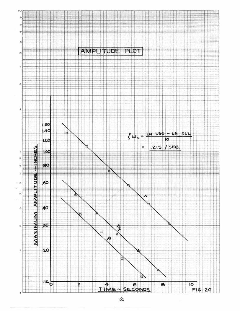
4. Amplitude Plot 15
5.' Vector Diagram of Oscillation Components 17
6. Side-Force Vector Diagram 18
7. Rolling-Moment Vector Diagram 19
8. Yawing-Moment Vector Diagram 21
9. Rolling-Subsidence Mode Separation 22
10. Instrument Orientation Diagram 25
11. Fighter Airplane Instrument Geometry 36
12. Phase and Amplitude Corrections 38
13. Side-Force Vector Diagram 43
14. Rolling-Moment Vector Diagram 46
15. Phase Corrections 47
16. Yawing-Moment Vector Diagram 49
17. Flight Transient Records 58
18. Fighter Airplane, Three-View Drawing 59
19. Phase Plot 60
20. Amplitude Plot 61
vi

LIST OF TABLES
Table Page No.
1. Measured Phase and Amplitude Relationships 36
2. Corrected Phase and Amplitude Relationships 3%8
3. Comparison Between Extracted Derivatives and
Manufacturer's Estimates 50
4. Comparison Between Derivatives Extracted by the
Time-Vector and Ref. 6. Methods 53
viij
I. SUMMARY
This report presents a time -vector method for extracting the
lateral stability derivatives of an airplane from transient flight data.
The method has been developed from a consideration of the properties
of rotating vectors. The relationships between the phases and ampli-
tudes of the multiple degrees of freedom of a linearlly oscillating
system are time-invariant. That fact forms the basis of the time-vector
method.
The lateral oscillation of a fighter airpland was analyzed. The
analysis and sample calculations are presented in the appendix. It was
shown that relationships between the stability derivatives could be de -
rived which were commensurate, with the accuracy of the transient data.
The lateral oscillation provided sufficient conditions to evaluate five of
the seven lateral stability derivatives in terms of the other two. A
reasonable estimate for two of the derivatives gave good results for the
others. A similar analysis of the rolling-subsidence and the spiral
modes presents the two additional conditions which are necessary to a
unique solution for all derivatives.
The time-vector method of analysis is direct and easily applied.
The graphical solution permits an insight into the physical character of
the oscillation. That quality facilitates the detection and correction of
any inconsistencies that may be present in the data.
I

II. INTRODUCTION
A. A Discussion of the Problem
This report considers the application of a time-vector method to
the extraction of the lateral stability derivatives of an airplane from
transient flight data. The problem of determining stability derivatives
directly from dynamic flight tests has received considerable attention
in recent years. A brief background of the subject follows:
The basis for the study of airplane dynamics was introduced by
Bryan in 1911, Ref. 1. His mathematical description of the fixed-
control motion of an airplane remains fundamentally unchanged.
The fixed-control motion of an airplane is mathematically
described by six simultaneous, linear, differential equations with con-
stant coefficients. The equations are written for axes that are fixed in
the airplane. They are derived with the assumption of small disturbances
from an equilibrium flight condition. By virtue of airplane symmetry
and the restriction to small disturbances, the equations can be separated
into two groups which describe the longitudinal and the lateral motions.
The form of the lateral dynamic equations used in this report is presented
on page 12
The constant coefficients in the differential equations are called
stability derivatives. They represent a change in an aerodynamic force
or moment along, or about, one of the stability axis due to a departure
from equilibrium. Limitations to their use are discussed in texts on the
subject; one such text is Ref. 2.
2

Accurate estimates of stability derivatives are essential in the
design of an airplane in order to insure good flight characteristics.
Those estimates must be based on aerodynamic theory and, where
possible, wind-tunnel tests. It would be beneficial to the aerodynami-
cist if he were able to get a direct check on his estimates from dynamic
flight tests. Until recently, the only practical check available was a
comparison between a calculated and an actual flight response to a dis-
turbance. That check was not positive since compensating errors in the
derivatives could mask significant inaccuracies.
It should be noted that the lateral stability derivatives of a Bristol
fighter were extracted from flight tests by British investigators in the
1920's, ref. 3. Some similar work was done in this country in the
1930's and early 1940's. However, those methods were very difficult
to apply and hence were not used generally by aerodynamicists in industry.
The difficulties inherent in estimating stability derivatives
accurately were significantly increased with the use of highly swept
wings and the advent of transonic flight speeds. The need for methods
of checking estimated derivatives by dynamic flight tests of the com-
pleted airplane became more acute. The correlation between theory
and practice would permit improved estimates of stability derivatives
for advanced designs.
Considerable research effort has been expended in recent years
toward the development of methods for extracting stability derivatives
and stability performance functions from dynamic flight tests. Milliken
has discussed some of the results obtained at the Cornell Aeronautical
Laboratories in Refs. 4 and 5. A method developed at that installation
3

and applied in Ref. 6 is considered briefly in this report. The NACA
has devoted considerable effort to the problem. Various methods
developed in their laboratories are presented in Ref. 7 through 11.
There are many other papers relating to the subject. The reader is
referred to the more extensive bibliographies contained in the referenced
documents.
This report is concerned principally with a time -vector method
for extracting stability derivatives from transient flight data. The method
is especially applicable to lightly-damped, oscillating systems. It is
applied herein to the extraction of the lateral stability derivatives of a
fighter airplane by analyzing its lateral oscillation.
The rotating vector diagram employed in the method has been used
by electrical engineers for many years. The first known application in
aeronautics was by Mueller of MIT in 1937, Ref. 12. He-used it to de-
termine the character of the longitudinal oscillatory modes of an airplane
when its stability derivatives and inertia properties were known. Thus,
he used it in the sense of synthesis. The principle lay dormant for
many years. It has been considered by several people since World War
II. Doetsch, a German scientist working in Great Britain, has prepared
a report, Ref. 13, in which he considers an application similar to
Mueller's in greater detail. He also applies the method in a synthesis
sense.
The time-vector principle has been recently applied in the sense of
analysis: the problem of determining the stability derivatives when the
transient motion of the airplane is known. The only thorough development
4
and application of the method known to the writer was that of Professor
Larrabee of MIT in Ref. 14. The development in this report closely
follows that of Professor Larrabee.
5
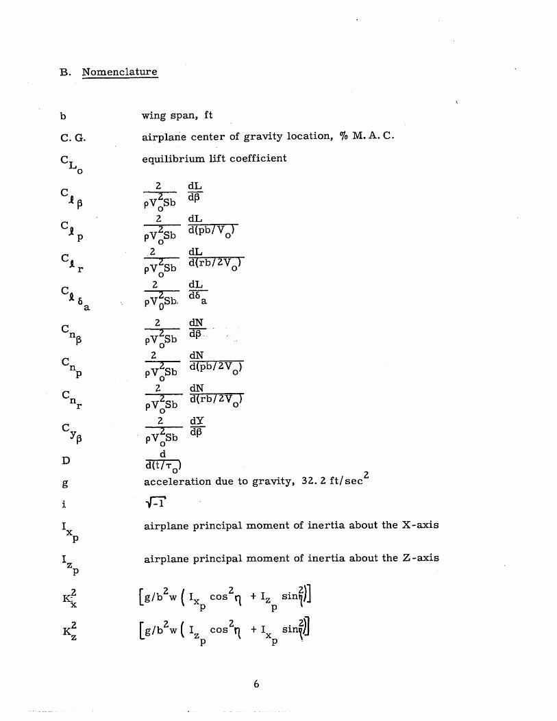
B. Nomenclature
wing span, ft
airplane center of gravity location, % M. A. C.
equilibrium lift coefficient
2 dL
pV 2 Sb dpb0
2 dL
pV2Sb d(pb/2V)
2 dL
pV 2 b d(rb/V
2 dL-- aU-
pV0 Sb, a
2
pV S$b2
pV2 Sb0
2
pV2Sb0
2
pV0 Sb
dd(t/T)
dN
dNd(pb/2V0)
dNd(rb/ZVT)0
dYd 0
acceleration due to gravity, 32. 2 ft/sec2
airplane principal moment of inertia about the X-axis
airplane principal moment of inertia about the Z-axis
g/bw ( I. Cos2q + Iz sin
[g/b 2 w ( I2Cos +I sin 2
p
6
b
C. G.
CL0
C p
C p
C r
C aa
C
Cnp
Cnr
CYp
D
g
i
Ixp
zp
2K:x
K 2z

K g/b 2 w (Iz - x ) sin rt cos rip p
L rolling moment, ft-lbs
M Mach number
M. A. C. mean aerodynamic chord, ft
N yawing moment, ft-lb
lateral acceleration in g's
OAT outside air temperature, 0F
p angular velocity about X-axis, rad/sec
r angular velocity about Z-axis, rad/sec
S wing area, ft
t time, sec
Vc calibrated airspeed
Vi indicated airspeed
V0 equilibrium true airspeed
W gross weight, lb
Y side force, lb
a angle of attack, deg
P angle of sideslip, rad
o( flight path angle, rad
6 pressure ratio, ambient/sea level
6 total aileron angle, deg
eD sin~I,, damping angle, rad
0 angle of roll, deg
7

p phase angle of p relative to P, deg
phase angle of n relative to P, degn y
r phase angle of r relative to p, deg
rolling subsidence mode root
X ~spiral mode root
M pbairplane density parameter
angle between principal axis and stability axis
angular velocity of oscillation, rad/sec
Won undamped natural frequency, rad/sec
W . T W , nondimensional undamped natural frequencyn 0 on
p0 NACA std. sea level atm. density, slugs/ft3
atm. density ratio, ambient/sea level
b-rT ro , aerodynamic time reference, sec
9Q L airplane reference axis angle of zero lift, deg
angle of yaw, rad
lateral oscillation damping ratio
8

III. THEORY AND DISCUSSION
A. Properties of Rotating Vectors
Consider a freely oscillating system composed of a mass, a
viscous damper, and a spring. For small disturbances, its motion can
be described mathematically by a linear, second-order differential equa-
tion.
S-x + + k x= 0m-~-- dtdt
where
x = displacement
m = mass
c = damping constant
k = spring constant
If the damping of the system is less than critical, the roots of the
equation may be expressed as
-on- n
With initial conditions which eliminate one root,
- ont + iW ;1_-72 tx=x e n
The first derivative of x can be written:
~n ei(I X + 9g0 +e D)
9

where E.D = amping angle
= tan-
= sin~ -
Similarly,
fx dt ei(i - 900 - ED
n
Those quantities can be plotted as vectors in the complex plane.
Irni.dx n1Ika n %r
ReatX
a- W.~L W -
so C ., i
Wn
Fig. 1, Derivatives and Integrals of Vectors
The quantity x, its time -derivatives, and its integrals all rotate with the
same angular velocity, o, in the complex plane. Also, each of the vectors-Go t
has its magnitude decreased by the same multiplicative factor, e n it
follows that the relationships existing between the amplitudes and phases
of the vectors are not functions of time.
10

For the simple mass-spring-viscous damper system described by
the equation
mi + ci + kx = 0,
oscillatory solutions can be represented by closure of a vector in which
each of the terms is represented by a vector as shown in Fig. 2.
Fig. 2, Vector solution for one -degree -of -freedom oscillation
The concepts established for the one-degree-of-freedom system
can be extended directly to a system. with multiple degrees of freedom.
All components of the system, and all derivatives and integrals of the
components, will rotate with the same angular velocity and decay with
time by the same factor. Hence, phase and amplitude relationships be-
tween the components of a linearly oscillating, multiple-degree-of-freedom
system are time-invariant. That conclusion is important; it is the foun-
dation of the time-vector method for analyzing oscillating systems. The
phase and amplitude relationships between the components to comprising
the motion may be determined by considering the oscillation frozen at any
11
instant. The relationships may be used to solve for the constant
coefficients of the linear differential equations which describe the com-
plete oscillation.
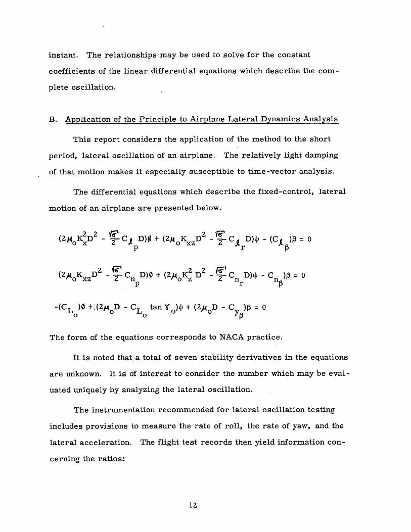
B. Application of the Principle to Airplane Lateral Dynamics Analysis
This report considers the application of the method to the short
period, lateral oscillation of an airplane. The relatively light damping
of that motion makes it especially susceptible to time-vector analysis.
The differential equations which describe the fixed-control, lateral
motion of an airplane are presented below.
ox 1 2 Z Cj D)0+ (2AK D- TC D)J (CA2 2 0 x 2 19'
(2#OK D - i" Cn D)0 + (ZAOK 2D - C D) -C 0
p r p
-(CL )0 +((2p D - CL tan Y )qj + (24 0 D - C )p = 0
The form of the equations corresponds to NACA practice.
It is noted that a total of seven stability derivatives in the equations
are unknown. It is of interest to consider the number which may be eval-
uated uniquely by analyzing the lateral oscillation.
The instrumentation recommended for lateral oscillation testing
includes provisions to measure the rate of roll, the rate of yaw, and the
lateral acceleration. The flight test records then yield information con-
cerning the ratios:
12
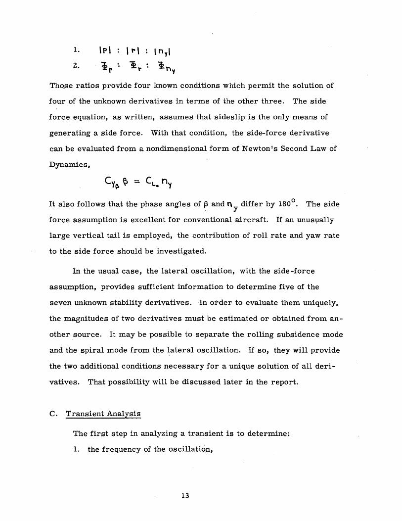
Those ratios provide four known conditions which permit the solution of
four of the unknown derivatives in terms of the other three. The side
force equation, as written, assumes that sideslip is the only means of
generating a side force. With that condition, the side-force derivative
can be evaluated from a nondimensional form of Newton's Second Law of
Dynamics,
It also follows that the phase angles of P and n differ by 180. The sidey
force assumption is excellent for conventional aircraft. If an unuspxally
large vertical tail is employed, the contribution of roll rate and yaw rate
to the side force should be investigated.
In the usual case, the lateral oscillation, with the side-force
assumption, provides sufficient information to determine five of the
seven unknown stability derivatives. In order to evaluate them uniquely,
the magnitudes of two derivatives must be estimated or obtained from an-
other source. It may be possible to separate the rolling subsidence mode
and the spiral mode from the lateral oscillation. If so, they will provide
the two additional conditions necessary for a unique solution of all deri-
vatives. That possibility will be discussed later in the report.
C. Transient Analysis
The first step in analyzing a transient is to determine:
1. the frequency of the oscillation,
13

2. the damping ratio,
3. the relationship between the amplitudes of the degreesof freedom,
4. the relationship between the phase angles of the degreesof freedom.
That information can be obtained by plotting the oscillation data in the
following manner:
First, plot the times at which all components of the oscillation
cross the zero axis as shown in Fig. 3.
sec,U
0 TtME ~ SEC.
Fig. 3, Frequency Plot
The common slope of the curves of Fig. 3 precisely determines the
frequency and the period of the oscillation. The horizontal distance be-
tween the curves provides the relationship between the phase angles of
the degrees of freedom. The data points for each oscillatory component
14
Is
should generate a straight line. If they do not, it is an indication that
nonlinearities are present.
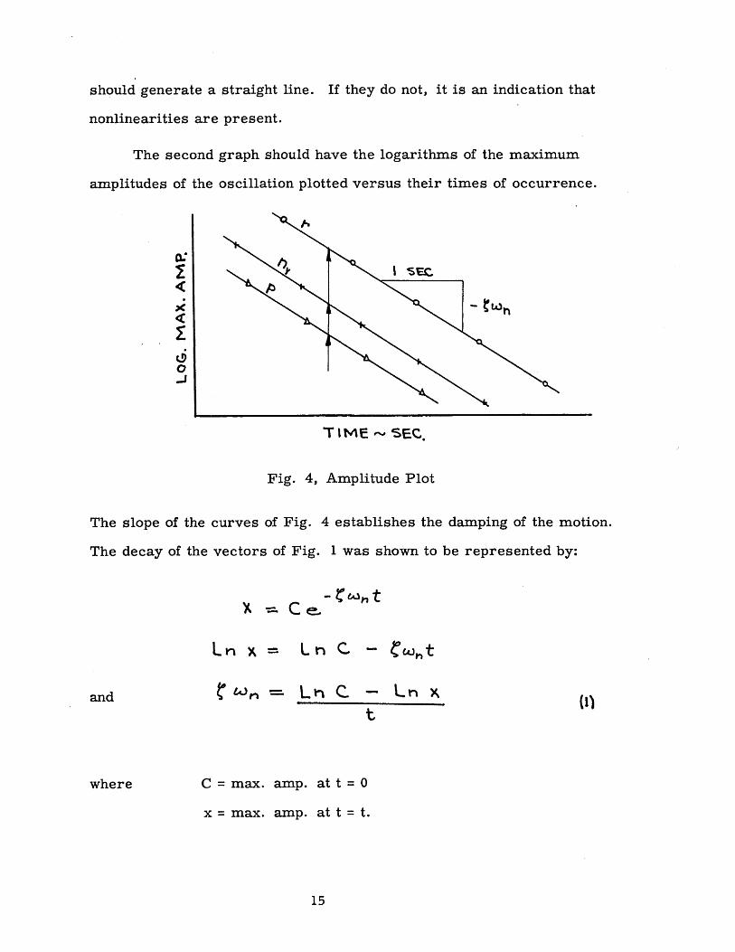
The second graph should have the logarithms of the maximum
amplitudes of the oscillation plotted versus their times of occurrence.
CSE
0
TIME~ SEC.
Fig. 4, Amplitude Plot
The slope of the curves of Fig. 4 establishes the damping of the motion.
The decay of the vectors of Fig. 1 was shown to be represented by:
Ln x = Ln C -
and n L ri C- - Lt
where
(It)
C = max. amp. at t = 0
x = max. amp. at t = t.
15

Also recall that
The values of the damping ratio () and the undamped natural
(wn) can be solved with relations (1) and (2).
The relative amplitudes of the degrees of freedom may
ascertained by considering the motion frozen at any instant.
tude relationships may be determined along vertical lines as
Fig. 4.
frequency
be
The ampli-
shown in
Misalignments of the rate instrument input axes and improper
location of the lateral accellerometer have significant effects on the
measured phase and amplitude relationships. When those conditions
exist, corrections must be applied to the data. A method of correcting
phase and amplitude relationships for instrument geometry is given on
page 24
The corrected data can be presented as a vector diagram in the
complex plane. The general appearance will be that of Fig. 5. It was
shown that measuring p is usually unnecessary. The phase of p can be
considered to differ from that of ny by 1800. The nagnitude of p can be
established by the side-force vector diagram. That is indeed fortuitous
since sideslip is inherently difficult to measure accurately.
16
LW = Wn (a~

dt= roll
r ate.
I atet-allaccell,
9 sabe-siangle
=ryaw rafedit
Fig. 5, Vector Diagram of Oscillation Components
D. Construction of the Vector Diagrams
It is convenient to consider the side-force equation first. It may
be written as
CYfS+ CLO
Construction of the side-force diagram facilitates critism of the transient
data. The magnitudes of all terms on the right hand side of the equation
are known. It is not uncommon for the vector diagram to fail to close.
The appropriate adjustment is to alter the phase of r with respect to p
17
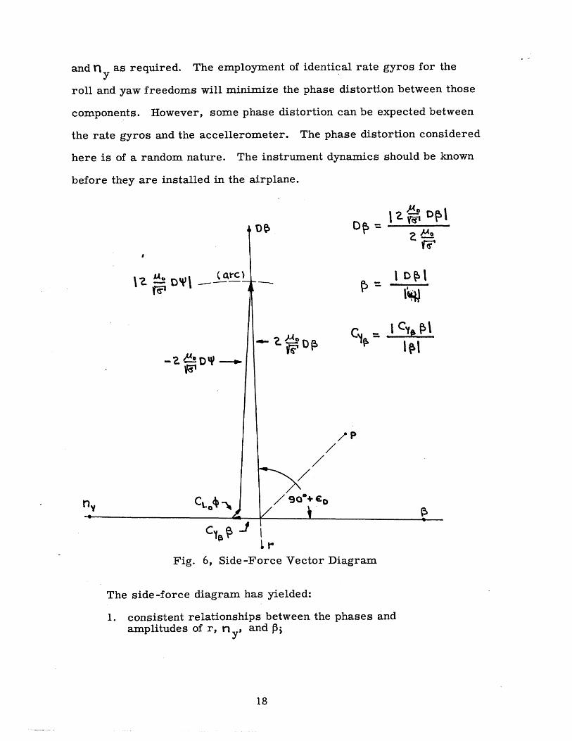
and ri as required. The employment of identical rate gyros for they
roll and yaw freedoms will minimize the phase distortion between those
components. However, some phase distortion can be expected between
the rate gyros and the accellerometer. The phase distortion considered
here is of a random nature. The instrument dynamics should be known
before they are installed in the airplane.
02
- I D~II.Z D'Y~S3c)
MO IY0-Z-DW
n.y CLOC_4) \/9iD
Fig. 6, Side-Force Vector Diagram
The side-force diagram has yielded:
1. consistent relationships between the phases andamplitudes of r, ry , and pi
18

2. the magnitude of C ;
3. an opportunity to criticize the accuracy of the phaseand amplitude data.
The rolling-moment equation may be considered next. It is
convenient to write it:
2.Ao KZ D$- SC. DY + 2.A. KD' = X C,04+1
One of the three unknown stability derivatives must be estimated or
obtained from another source. The proper derivative to estimate will
depend upon the airplane configuration. CZ was considered estimatedr
in the equation above and in the diagram of Fig. 7.
44N.dt
Z -, KD4 .
-... c c 04
dt
Fig. 7, Rolling-Moment Vector Diagram
19
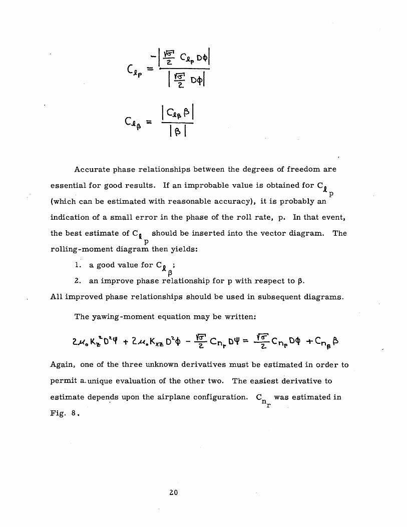
Cs =
Accurate phase relationships between the degrees of freedom are
essential for good results. If an improbable value is obtained for CIp
(which can be estimated with reasonable accuracy), it is probably an
indication of a small error in the phase of the roll rate, p. In that event,
the best estimate of C, should be inserted into the vector diagram. Thep
rolling-moment diagram then yields:
1. a good value for C ;
2. an improve phase relationship for p with respect to p.
All improved phase relationships should be used in subsequent diagrams.
The yawing-moment equation may be written:
E.K'LD2 + ZA.KxfD'4 - rCn0) 1n, -w-+Cn,(S
Again, one of the three unknown derivatives must be estimated in order to
permit a. unique evaluation of the other two. The easiest derivative to
estimate depends upon the airplane configuration. Cn was estimated inr.
Fig. 8.
Z0

Zjx.KI D E)
Cnpi
r-4
ZM K t~'4C
--- 4
Fig. 8, Yawing-Moment Vector Diagram
C = --- A
CnP C 2-'Cr p t6
INThe yawing-moment diagram has yielded:
1. the magnitude of Cnp
2. the magnitude of C n
An important feature of the time-vector method of transient analysis
should not be overlooked. Since it is a graphical solution, it permits a
visual consideration of the relative importance of the oscillation compon-
ents. The graphical constructions are easily checked by slide-rule
21
//
se+eb
r

calculations.
Data inconsistencies are easily discovered. The physical insight
afforded by the vector diagrams facilitates logical adjustments.
E. Consideration of the Rolling-Subsidence and the Spiral Modes
It has been noted that it is not possible to evaluate all of the lateral
stability with the lateral oscillation. Two derivatives had to be estimated
or obtained from another source. In some cases, it is possible to separ-
ate the rolling-subsidence and spiral modes from the lateral oscillation
in the flight record. If that can be accomplished, those modes will
supply the additional conditions necessary for a unique solution of all de -
rivatives. The difficulty lies in the accurate identification of the modes
which is essential to a good solution of their roots.
The rolling-subsidence mode may be extracted by back-figuring
the oscillations after their linear parameters have been established.
The difference between the record and the calculated motion is due to
the rolling-subsidence mode as shown in Fig. 9.
R o \\mq-subs idence.
C-ontg-buhonc
Fig. 9, Rolling -Subsidence Mode Separation
22
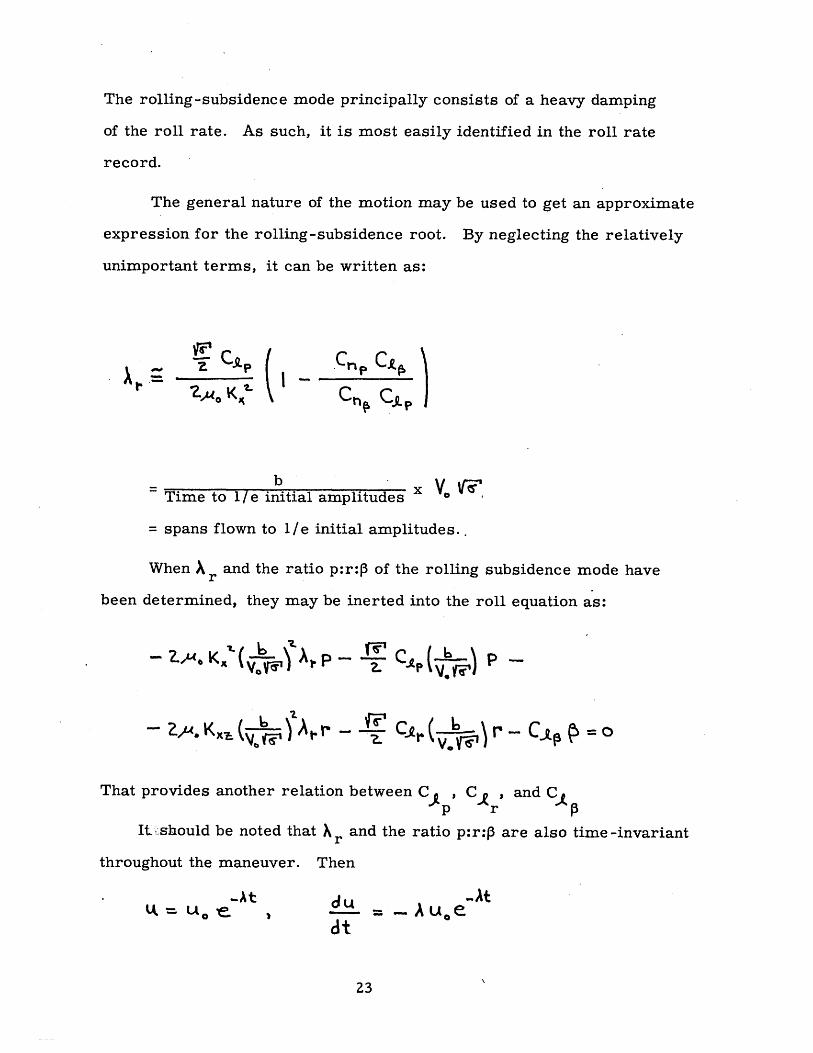
The rolling-subsidence mode principally consists of a heavy damping
of the roll rate. As such, it is most easily identified in the roll rate
record.
The general nature of the motion may be used to get an approximate
expression for the rolling-subsidence root. By neglecting the relatively
unimportant terms, it can be written as:
Iku K~ C,
b xVTime to 1/e initial amplitudes *
= spans flown to l/e initial amplitudes..
When A r and the ratio p:r:p of the rolling subsidence mode have
been determined, they may be inerted into the roll equation as:
That provides another relation between C , C , andCp r
It. should be noted that X and the ratio p:r:p are also time -invariant
rw
throughout the maneuver. Then
dt
23

and f L( dt e .
The spiral mode is easily identified if the oscillation
is allowed to continue for a sufficient period. However, the
time required to develop a reasonable amplitude is usually so
great the atmospheric turbulence becomes a significant factor.
Since the motion grows or subsides so slowly, it is advisable
to measure roll angles and headings since
P
The spiral root and the ratio p:r:o may be inserted into the
yawing-moment equation to give another relationship between
C h, Ch , and C.
An approximate functional relationship may be written
for Xs as: ( . C
Wr Cot.crjp C11.
~~.r is C~, CraP Cns + CAP' ~
b y___r_Time to e initial amplitudes if unstable *
spans flown to e initial amplitudes.
F. Corrections for Instrument Orientations and Locations
Roll rates and yaw rates should be measured about the
airplane stability axes; lateral accelleration should be meas-
ured at the airplane center of gravity normal to the plane of
symmetry. The usual flight test
24

instrumentation has the accellerometer aligned in the proper direction.
It is often impractical to fulfill the other conditions.
The X-stability axis is initially aligned with the equilibrium flight
direction; its relationship to the airplane center line is a function of
airplane angle of attack. It would not be practical to make frequent
changes in the roll rate and yaw rate instrument orientations.
The airplane center of gravity may not be accessible for instrument
installation. For example, it may be located inside a fuel cell. In that
event, the lateral accellerometer should be located as near to the air-
plane center of gravity as is possible.
The measured quantities may be corrected for instrument geometry
as shown below
Y o Accenlerome er
hxA
Fr
Fig. 10, Instrument Orientttion Diagram
25
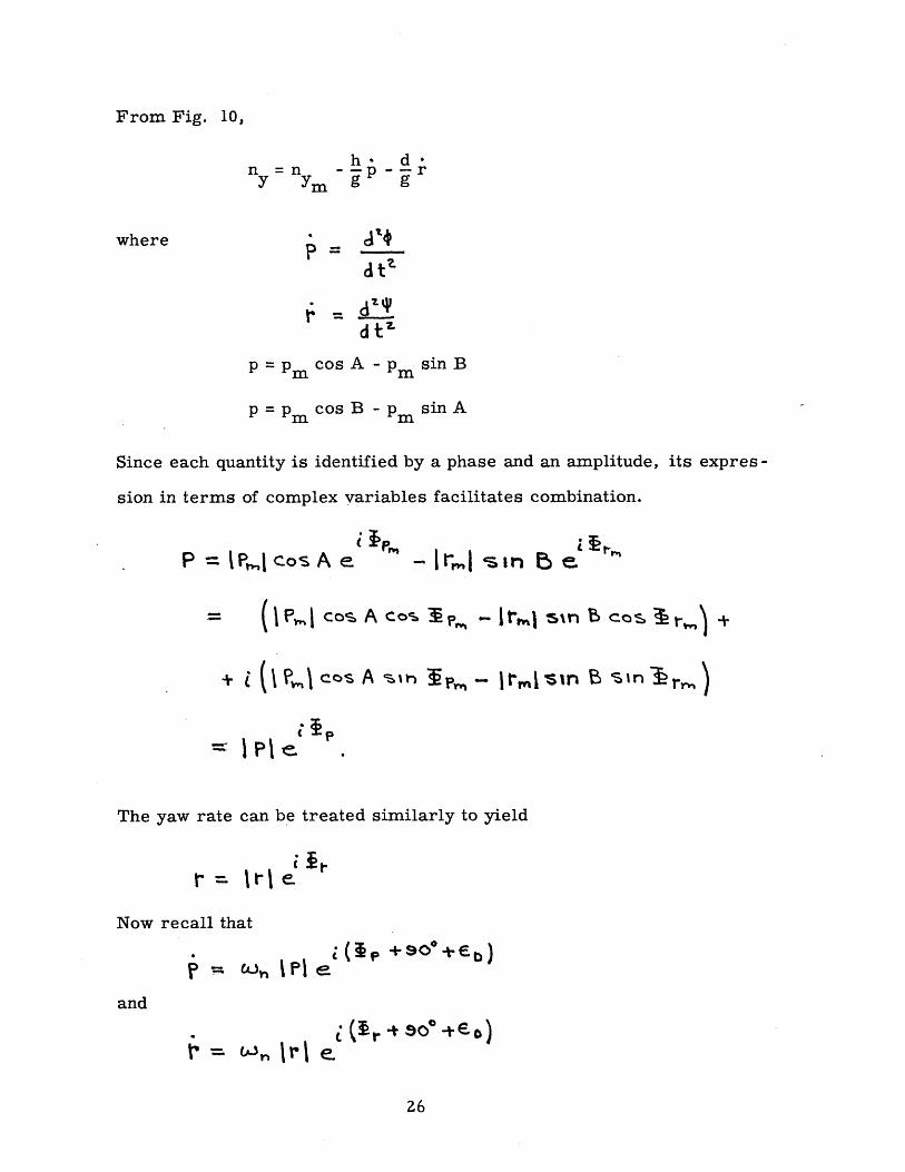
From Fig. 10,
n =n
whereP
h - d --- p -- r
dI
a tz
p pmcosA -pm sinB
p PMcosB -p msinA
Since each quantity is identified by a phase and an amplitude, its expres -
sion in terms of complex variables facilitates combination.
P = IP cos A e - Iri Sin b e
= 0 P,. cos A cos IP,
The yaw rate can be treated similarly to yield
r- - It-I e. ft.
Now recall that
L = I~PI
and
W,~r Ir e-
(~p +~O±Eb)
c (~rO 0 *E~c~)
26
IrMI so b cos l --Q) +
Irrnisrn eB sinr,,i)
e
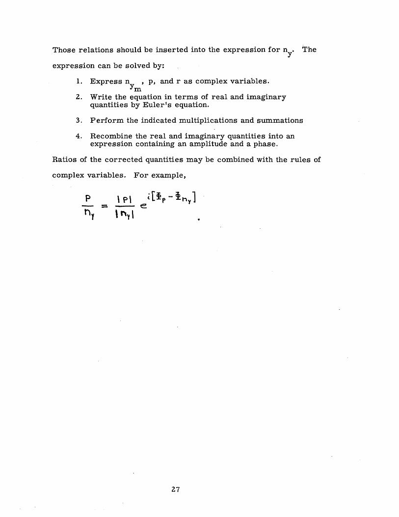
Those relations should be inserted into the expression for n . The
expression can be solved by:
1. Express n , p, and r as complex variables.
2. Write the equation in terms of real and imaginaryquantities by Euler's equation.
3. Perform the indicated multiplications and summations
4. Recombine the real and imaginary quantities into anexpression containing an amplitude and a phase.
Ratios of the corrected quantities may be combined with the rules of
complex variables. For example,
P lel Y
27

IV. CONCLUSIONS
The following conclusions may be derived from a consideration
of the preceding development and the sample calculations of the analysis
presented in the appendix.
1. The time-vector method of analyzing a linear, multiple-degree-
of-freedom, oscillatory system is straight-forward and easily applied.
It is especially applicable to the analysis of lightly damped systems. It
yields relationships between the stability derivatives of an airplane which
are commensurate. with the accuracy of the transient data. The assump-
tion of reasonable values for some derivatives yields good values for the
others. An analogous application of the method to the rolling-subsidence
and spiral modes permits a unique solution for all of the derivatives.
2. The method of plotting the transient data provides:
(a) the period and frequency of the oscillation,
(b) the damping of the oscillation,
(c) relationships bet'ieen the phases and the amplitudesof the oscillatory components.
It also indicates any deviations from linearity. Similarly, it permits the
averaging of any experimental scatter which may exist.
3. The method fully exploits the linear qualities of the transient
data of a system which may be described mathematically by a set of
simultaneous, linear, differential equations.
4. The graphical solution clearly indicates the presence of any
inconsistencies in the data. It also assists the engineer in determining
the proper adjustment.
28
5. It was noted that errors due to instrument misalignment or
location are significant. A method was developed for correcting those
errors.
29

V. REFERENCES
1. Bryan, G. H. , Stability in Aviation, 1911.
2. Duncan, W. J., The Principles of the Control and Stability of
Aircraft, Cambridge at the University Press, 1952.
3. Garner, H. M. and Gates, B. A., "Full Scale Determination of
the Lateral Derivatives of a Bristol Fighter Airplane, " Br. A. R. C.
R. and M. 987, 1925.
4. Milliken, W. F. , Jr., "Progress in Dynamic Stability and Control
Research, " Journal of the Aeronautical Sciences, Vol. 14, No. 9,
p. 493, September 1947.
5. Milliken, W. F., Jr., "Dynamic Stability and Control Research,"
Cornell Aeronautical Laboratory Report No. 39, September 1951.
6. Segel, L., "Dynamic Lateral Stability Flight Tests of an F-80A
Airplane by the Forced Oscillation and Step Function Response
Methods, " Cornell Aeronautical Laboratory Report No. TB-495-F-13,
April 1950.
7. Greenberg, Harry, "A Survey of Methods for Determining Stability
Parameters of an Airplane from Dynamic Flight Test Measure-
ments, " NACA Technical Note 2340, U. .S. Government Printing
Office, April 1951.

8. Shinbrot, M. , "A Least-Squares Curve-Fitting Method With
Applications to the Calculation Transient Response Data, " NACA
Technical Note 2341, U. S. Government Printing Office, April
1951.
9. Donegan, J. and Pearson, H. A., "A Matrix Method of Determining
the Longitudinal-Stability Coefficients and Frequency Response of
and Aircraft from Transient Flight Data, " NACA Technical Note
2371, U. S. Government Printing Office, June 1951.
10. Shinbrot, M., "An Analysis of the Errors in Curve-Fitting Pro-
blems With Application to the Calculation of Stability Parameters
from Flight Data, " NACA Technical Note 2820, U. S. Government
Printing Office, November 1952.
11. Donegan, J. J., "Matrix Methods for Determining the Longitudinal-
Stability Derivatives of an Airplane from Transient Flight Data,
NACA Technical Note 2902, U. S. Government Printing Office,
March 1953.
12. Mueller, R. K., "The Graphical Solution of Stability Problems,"
Journal of the Aeronautical Sciences, Vol. 4, p. 324, June 1937.
13. Doetsh, K. H. , "The Time-Vector Method for Stability Investiga-
tions," Royal Aircraft Establishment Report, Aero 2495, Great
Britain.
14. Larrabee, E. E., "Application of the Time-Vector Method to the
Analysis of Flight Testt Lateral Oscillation Data, " Cornell Aeronautical
Flight Research Department Memorandum No. 189, Sept. 9, 1953.
31

VI. APPENDIX
A. Sample Calculations of a Time-Vector Analysis of a Lateral
Oscillation
1. General Discussion
The time-vector method was used to extract the lateral stability
derivatives of a fighter airplane from its lateral oscillation. A three-
view drawing of the airplane is presented on page 59 . The lateral
oscillation was excited by a rudder pulse; a representation of the flight
record is shown on page 58
2. Flight conditions
w = 12,880 lb, s =237. 6 ft 2
2= 12, 540 slug-ft , b =38. 9 ft
xp
I = 31,000 slug-ft2
p
C. G. position: 25. 6% M. A. C.
Altitude: 20, 000 ft
V. = 260 MPH
OAT = +3 0F
3. Calculation of flight constants
(a) It must be assumed that Vi = Vc since no airspeed calibration
data were available.
Then,
M = 493V0 = Ma
(. 493)(1116)(. 944)= 519 ft/sec
32

(b) CL = 2o 1481 M 6 S
12, 880
(1481)(. 493)2(. 459)(237. 6)
. 328
(c) m pSb
12, 880~ (32. 2)(. 002378)(237. 6)(38. 9)
18. 18
b
38. 9(.-718)(519).
. 1045 sec
4. Flight attitude
Flight measurements indicated that 901
CL5. 10 per radian
= -1. 70
5. 1057. 3
= .089 per degree
33
(d)

0= CL
(-)
.328
.089- 1. 7
=3. 69 - 1. 7
0 T 20
The X principal axis of inettia is estimated 4 0 blwthe reference
axis of the airplane.
q~ = +20.
5. Inertia constants
K 4,= ( )2(I)x mP
_ (12540)(32. 2)~2
(38.9) (12880)
-. 0207
K 2 2)z b mp
(31, 000)(32. 2)
(38. 9) (12880)
= .0512
+20
2- 2
K2 =Kx p
2 2cos + K
p
34
Then
For q =
s 2sinq
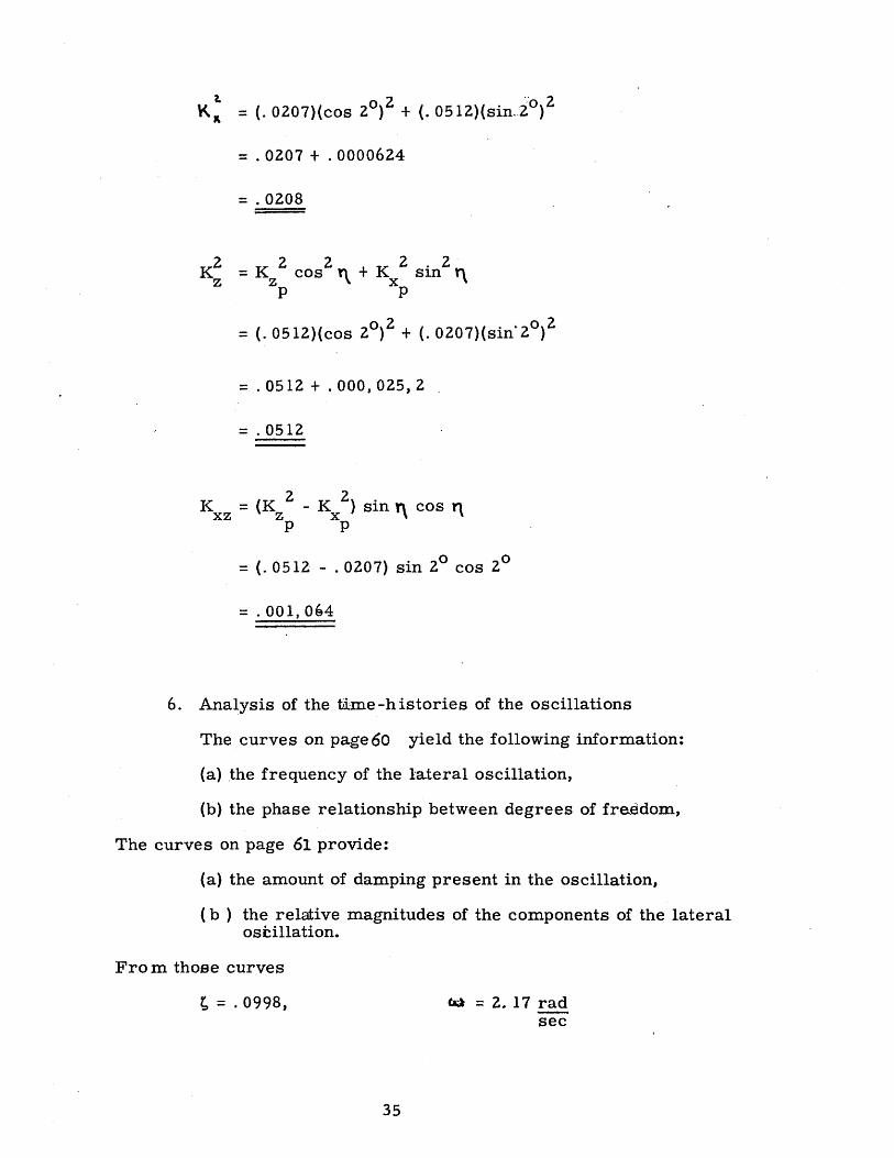
z 2 o 2K = (.0207)(cos 2) + (. 0512)(sin..-2
. 0207 + . 0000624
. 0208
2 2 2 2.2K = Kz cos 2r + K sin \
p p
= (.0512)(cos 20)2 + (. 0207)(sin'20)2
= .0512 + .000, 025,2
= .0512
2 2K = (Kz - K ) sin rt cos rl
p p
(.0512 - . 0207) sin 20 cos 20
= .001, 064
6. Analysis of the time-histories of the oscillations
The curves on page60 yield the following information:
(a) the frequency of the lateral oscillation,
(b) the phase relationship between degrees of freedom,
The curves on page 61 provide:
(a) the amount of damping present in the oscillation,
(b ) the relative magnitudes of the components of the lateralostillation.
From those curves
S=.0998, ta =2. 17 radsec
35

Table 1, Measured Phase and Amplitude Relationships
Measured Quantity
p
r
ny
Amplitude Relationships
.0664 rad/sec
.0736 rad/sec
.0218 g's
Phase Angle Relationships
144. 3 deg.
265.5 deg.
180 deg.
Those relationships must be corrected for the orientation of the
input axes of the roll rate and yaw rate gyros, and for the location of
the lateral accellerometer with reference to the airplane center of gra-
vity. The instrument orientations and locations are shown below.
G.01 ft.
0 Accellerore+er
.15 ft.
x P-C.G.
Fig. 11, Fighter Airplane instrument Geometry
36

Dp =PM
p =r
n =nY ym
S75g
p
= sin -
= 5.80
6.08g
p = &n IP ei(p
= (2. 17 rad/sec)(
+ 900 + E )
. 0664)ei( 144. 3 + 90 + 5. 8)
= . 144 rad/sec2 at 240. 10
r = 'n I r e Or+ 900 + E)
= (2. 17 rad/sec)(. 0736)e i(265. 5 + 90 + 5. 8)
2 0-. 159 radlsec .at + 1. 3
(.75)(. 144)e i ( 240.
32. 2Z
1i0) (6. 08)(. 159)e i 1. 30)32. 2
= .0218 ei (180 0 ) -. 00336 e i (240. 10) - . 0300 e i (1. 30)
= . 0502 at 177. 50
Fig. 12 shows the vector relationships before and after correction for the
instrument orientations and location.
37
n =nY Y

?=Fv =.0rr.4 sad.se..
I=OZIB 9's
I-adI.r~ r 11(c
Fig. 12, Phase and Amplitude Correction
Rotation of the vector diagram so that the phase of n is 1800 gives:
Table 2, Corrected Phase and Amplitude Relationships
Amplitude
.0664 rad/sec
.0736 rad/sec
. 0502 g's
Phase
146.8
268
1800
The angular velocities must be nondimensionalized for insertion
into the equations of motion presented on page 12 .
38
Quan.
p
r
ny

d0p o = -(A)n T
= (. 1045)(2. 17)
DO - t/r) . 226
d00 dt
= (.1045 sec)(. 0664 rad/sec)
= . 00694 at 146. 8
D = - d-=T 0 rD$=-o =t -r0
= (. 1045)(. 0736)
. 00770 at 2680
Those relationships, with the nondimensional lateral accelleration should
be suitable for use in the final solution of the problem.
7. Discussion of the validity of preceding results
A preliminary analysis, including diagrams, indicated that the
supporting data and the actual transient recrods were not compatible. An
extensive check of the supporting data, such as airplane weight, inertias,
instrument locations, calibrations, and dynamics, was in order. Un-
fortunately, the flight test had been conducted in 1951; therefore, it was
not possible to accomplish those checks. It then became necessary to
determine the most logical correction to the data which would be con-
sistent with the transient records and with information on the stability
derivatives obtained from other sources.
39

A study indicated that the following changes were most probable:
(a) n = . 0073 instead of . 0502
(b) k = 8. 81 ft. instead-of 9. 85 ft.
(c) k = 5. 60 ft. instead of 5. 69 ft.x
-Those changes can be shown to be reasonable.
The lateral accelleration could have been inaccurate for one or
more of the following reasons:
(a) The instrument calibration could have been incorrect.
(b) Improper excitation voltage may have been used whenthe test condition was recorded.
(c) The accellerometer location relative to the airplaneC. G. may not have been accurately known.
(d) The accellerometer input axis may have been mis-aligned.
Moments of inertia have very significant effects on the damping and
the period of the lateral oscillation. An accurate knowledge of the inertias
is thus important. The inertia data received with the flight test records
were not considered especially accurate. It became apparent in the analy-
sis that either Iz of the damping of the oscillation had to be reduced in
order to obtain reasonable yawing moment derivatives from the rest re-
cords. Determination of the damping of the oscillation from the time -
histories was straight -forward and considered reliable. Consequently,
the airplane moment of inertia about the Z-axis had to be reduced. There
are no independent inertia data for the airplane considered which are
available for a check. However, the corrected inertias appear reasonable
when compared to those of geometrically similar airplane.
40

8. Calculation of the stability derivatives by means of vectordiagrams
(a) Side-force diagram
From page 12
2MA~-- Dp = C y
yp
0 = en
. 00694. 226
= . 037 at
, the side-force equation is:
D$
D9 - 900 -E D
ei (146.8 - 90 - 5.8)
51. 00
0 = (.328)(. 0307)
= .01007 at 51.0 0
D$ = (2)(18. 2) (.00770).718
= . 390 at 2680 (The phase angle will be checkedin the diagram).
_ (2)(18. 2).718
= 50. 6 Dp
Since side force is almost entirely a result of sideslip, it is reasonable
to assume that n and P have a phase difference of 1800. Then, the phase
41
CL0
2 M0
2po
L 9 + 2 -- 0-L0 -V_
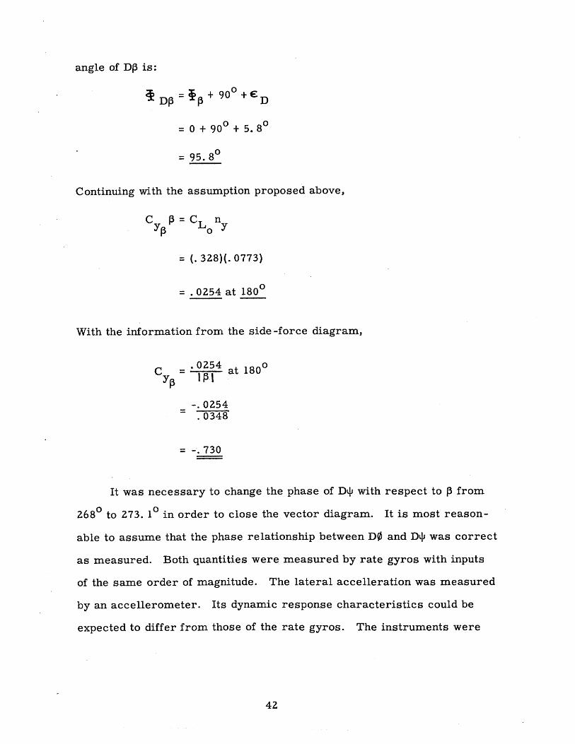
angle of DP is:
DP =p + 90 + E D
= 0 + 900 + 5.80
= 95. 80
Continuing with the assumption proposed above,
Cp=CL nyp L 0 y
= (.328)(. 0773)
= .0254 at 1800
With the information from the side -force diagram,
C = at 1800yp I p-1
-. 02540348
= -. 730
It was necessary to change the phase of D$i with respect to p from
2680 to 273. 10 in order to close the vector diagram. It is most reason-
able to assume that the phase relationship between DO and D$ was correct
as measured. Both quantities were measured by rate gyros with inputs
of the same order of magnitude. The lateral accelleration was measured
by an accellerometer. Its dynamic response characteristics could be
expected to differ from those of the rate gyros. The instruments were
42

S DO.6
O0
.coo-8.22.6a
' /o
++C= o
c.C , p ,ao zs4
Fig. 13, Side-force vector diagram
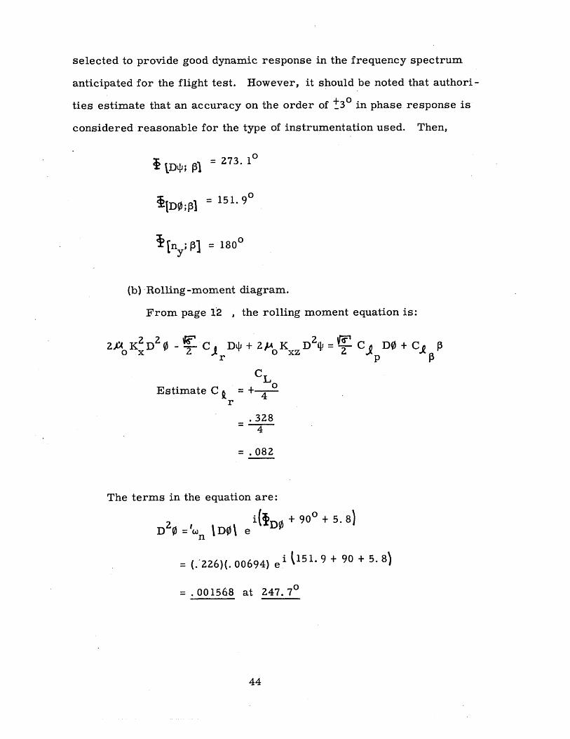
selected to provide good dynamic response in the frequency spectrum
anticipated for the flight test. However, it should be noted that authori-
ties estimate that an accuracy on the order of t3 0 in phase response is
considered reasonable for the type of instrumentation used. Then,
{D$; p= 273. 10
(D0;pI = 151. 90
In y;p = 1800
(b) Rolling -moment diagram.
From page 12 , the rolling moment equation is:
2 2 2 T2XAK D 0- Cj DL+ 2PK YD2 = Cg DO + CSO 2 r pCL
Estimate C 0
r
.3284
= . 082
The terms in the equation are:
D 2 = DD + 900+ 5.8)
(.'226)(. 00694) e i (l51. 9 + 90 + 5. 8)
=.00 1568 at 247. 70
44
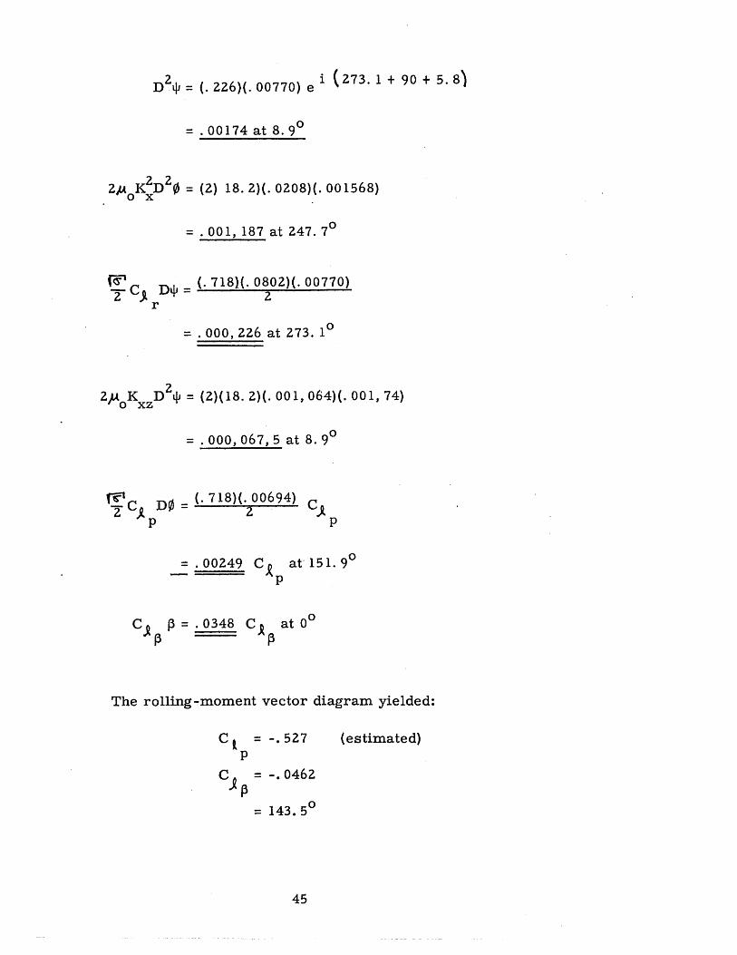
2 i ( 273. 1 + 90 + 5. 8)D =.226)(. 00770) e
- 00174 at 8.9 0
2)A K D 00ox
SC r
2pK D2@
= (2) 18. 2)(. 0208)(. 001568)
.00 1, 187 at 247. 70
(.718)(. 0802)(. 00770)2
= . 000, 226 at 273. 10
= (2)(18. 2)(. 001, 064)(. 001, 74)
= 000, 067, 5 at 8. 90
= (.718)(. 00694) C2 C
p
= . 00249
C = .0 3 48
C Ap at 151. 90
at 00
The rolling-moment vector diagram yielded:
C = -. 527 (estimated)p
C = -. 0462
= 143. 50
45
C DO~P

CAP -. 0029P .00o2.49
00160e8.0o348
- 0462.
i . P
+ CC, a
46 -6 . 5
Fig. 14, Rolling-moment Vector Diagram.
*x
+-p.e D
-TCr IDT
10 ) J]
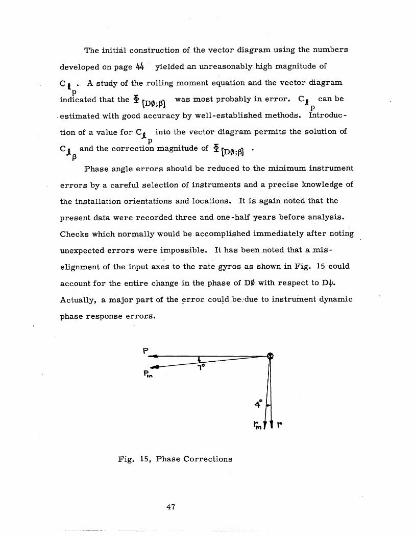
The initial construction of the vector diagram using the numbers
developed on page 44 yielded an unreasonably high magnitude of
C . A study of the rolling moment equation and the vector diagramp
indicated that the I {D0;P) was most probably in error. C, can be
estimated with good accuracy by well-established methods. Introduc-
tion of a value for CI into the vector diagram permits the solution ofp
C, Pand the correction magnitude of I {D0;p)*
Phase angle errors should be reduced to the minimum instrument
errors by a careful selection of instruments and a precise knowledge of
the installation orientations and locations. It is again noted that the
present data were recorded three and one-half years before analysis.
Checks which normally would be accomplished immediately after noting
unexpected errors were impossible. It has been noted that a mis-
elignment of the input axes to the rate gyros as shown in Fig. 15 could
account for the entire change in the phase of DO with respect to D4.
Actually, a major part of the error could.beedue to instrument dynamic
phase response errors.
4*
Fig. 15, Phase Corrections
47

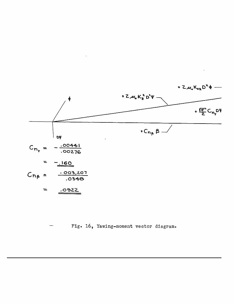
(c) Yawing-moment diagram
From page 12, the yawing-moment equation is:
&Z, K D ' + ZA4.Kx-D -- C D =
Again, one derivative must be estimated.
. Cr +C
For the airplane
considered,
t$ I
C OnCnP0
- oofli-
- oo15eet
call+n
o -4
o-t 8.4"
at '. .
Ot 2*a~ 0
2. I40 IL
At
2
= .000,O4O,(
Cn,.
.o~4e~ ~
o.t Z13.1 *
.-t O0
9. Summary of Results
The stability derivatives derived from the flight test are compared
with the manufacturer's estimates in Table 3.
48
CrI't
Sz.'K t a. z)(. o M. 2. )(. oo r014)
- . 00-2 .IS
+ W.A.KnD'4. Z-2.Knr
+ Cn,
C -0044-1
-. 160
. 00S,Z.0-.o34-8
- .092.2.
Fig. 16, Yawing-moment vector diagram.

Table 3, Comparison Between Extracted andturer's Estimates
Derivatives and Manufac -
Source
Mach No.
Altitude
Weight
C. G. pos.
Time -VectorAnalysis
. 50
20, 000 ft
12, 800 lb
25. 6% M.A. C.
Manufacturer'sEstimates
.60
20, 000 ft
14, 500 lb
27% M.A. C.
12, 540
31, 000
-. 73
-. 0462
-. 527
. 082 (est)
.0922
0 (est)
-. 160
Some additional information which were obtained from the transient
analysis are:
I1=
IZ.G2 o WL = 2..1 (
x
z
Cyp
C
C I
C Ir
Cn
Cnp
Cnr
26, 400
52, 200
-. 788
-. 066
-. 545
. 065
.093
.015
-. 136
S=.O99e,
read.Isec.
50
j:__b =
a.v.

Inyl
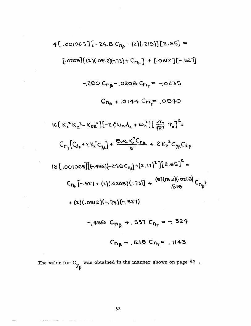
B. Lateral Oscillation Analysis by the Method of Ref. 6
The same rudder-pulse flight condition has been investigated using
the imethod of Ref. 6. It was not possible to determine all of the stability
derivatives since the airplane oscillation was not excited in the manner
most appropriate to that method of analysis.
The equations presented below have been taken from pages 19
and 20 of Ref. 6. The nomenclature has been changed to correspond
to that of this paper.
MCQP chi,
CA must be known. The method of Ref. 6 relies upon th measurementp
of the sideslip angle. The value obtained by the vector method will be
used in this analysis
o.C~e.,Cn,(j e2- m o
~ AreCn
Zx (7KCy,-+ C n,+K Ce)
51
i(.ooo6 '[- Z4..e c, - (z)(.zie))E z.6S)
Lozo()(osIz)(-:n)+l co) + {.os'z12[
--,tzo Co,-.OZOS Co,= --.oZas
Cn, + .o144 Cr .o i-o
%a
ZK c y + + Z Kt
nf ]l.'Sf =
+ (s(s)OO)Cr +
+ (sz-)
Cnr
Crh . ze Cn,
The value for CYp
was obtained in the manner shown on page 42 .
52
K6[ KK -Y, [Z % +4 E
6A(. K.,Cn ,Co n.C.V .
I1 .0o 1 oGS)(-.4%G)(-zISacn,) +(z.-
C nj {, -- 1 + -(1)(.o 0ZOS) t.-is))

-0.0~14 -
-, 12.8Cr'
I
I
I
I
.014~1-
*0~,4Q
* lI~~
- .1962.
030~3
.'144-
The solutions are seen to compare very well with those obtained by
the time-vector method.
Table 4, Comparison Between Derivatives Extracted by Time-Vectorand Ref. 5 Methods
Time -Vector
. 0922
-. 160
53
Cr U-
Method
C
Cnr
Ref. 6
. 0955
-. 1543
C. Rolling Subsidence Mode Analysis With Sample Calculations
The contribution of roll to the lateral oscillation considered in
the preceding analysis was small. The relatively small magnitudes of
the stability derivatives, C, and Cg , were responsible. The separa-
tion of the rolling-subsidence mode from the lateral oscillation was not
feasible.
A second test condition performed by the same airplane was
considered. Since the transient was initiated with an aileron pulse, a
relatively high roll rate was imposed at the beginning of the maneuver.
After the ailerons were returned to neutral, the maneuver was domin-
ated by the rolling-subsidence mode for approximately one second.
The test conditions are summarized below. Since similar
parameters were developed in detail for the lateral oscillation study,
only the results are listed.
w = 13, 830 lb
K =. 0273x
V = 315 MPH M = .592
ALT =20, 000 ft CL =. 244
o= 19. 6
T =.0869
V0 = 625 ft/sec
The analysis to be used assumes that only the rolling component
is significant in the rolling-subsidence mode. That assumption is justi-
fied by:
54

1. The initial roll rate is very large relative to theother motions.
2. CP and C are relatively small for the airplane
considered. C 'O.
It may be noted from the curves on page 58 that over -control
occurred when the ailerons were returned to neutral. The aileron
application opposite to the roll direction acted with the damping in roll
and must be considered.
With the assumption that only rolling motion was significant, the
present analysis could have been completed without quantitative knowledge
of instrument sensitivities if aileron over-control had not occurred.
However, it is necessary to know the aileron setting in order to ascer-
tain the contribution of the ailerons to the damping. Unfortunately,
the instrument sensitivity information for that particular test has been
lost. It is again noted that the tests were cnnducted in 1951.
Although the aileron over-control was small relative to the
magnitude of the pulse, its effect was significant. It was determined
that an initial total aileron angle over -control of one -half of one de -
gree, as shown on page 56 , provides a correction which gives a
reasonable value for Cp
The equation for pure rolling may be written
55

where Ddo
Sa4 so= t-)
An expression relating p and C is desired, wherep
Pdt
Solution of the differential equation for p gives:
C Sao t-1P = --
2 ,. m K , T"+z '
2 ' t,)t+ CONT. e
The constant can be evaluated with the initial condition, at t = 0,
p = 2. 05 inches of trace deflection.
CA_ S'a
Cj6Is .
After substitution,
+ T . _
{ Zm.KX' T- l +T
By inserting the values
Po = 39. 2
2K =.0273
T = . 5 sec
~1= . 716
T =.0869
CSa
= -. 126 per radian
6ao =. 5 degree = .00873 rad.
56
C-t\2PKZXe+ 7_Z.05 -

and the condition
p = . 63 inches at t = . 5 sec
the result C = -. 53 is obtained.
Although C compares favorably with the value used in thep
lateral oscillation, it si obviously not intended as a check. A pre-
knowledge of Cj was necessary to estimate the aileron contributionp
to the damping-in-roll. It had been expected that the analysis would
substantiate the magnitude of C, used in the lateral oscillation analy-p
sis. Calculations were essentially completed while a search was being
conducted for the instrument calibrations. The analysis does illus-
trate a method for evaluating C That is the only justification for itsp
inclusion in this report.
57

IIiiI

.C ....
Ie. F T
FIG. I8
59

--,-- ~ ~ ~ ~ ~ ~ 3 ---s~1~ ~--
* 1I-.--
z00
.:.4i
I _ _
Zv
__Io
x0,",
--4- --
xq
Ii
-I
* I I. .~ -.
'I<1 L
---4-- -
------T-
04- -~
b*1<
-I~j0110
i
I .......... I ------------ 4-
"0'
41
.
t - ..... .A .
I:1t74. r-~
~
'' I
-~
* .5
5- .5
- 1~
T,
[I;-;;;.4--5-v.',
4'
11 ..
... S
.
.4...
'till'
.4..
---
t
---
-----------
-+
---
+ .++r+
I- .
-+
+
.V
.
---
-..
-- 4
.4-
41
1--
g4
4 -
-
7Lt'
444 -
-4-4
--
14 4
4 -
--
-
p4i
4.1;1111
14
Ilk-.
I_ _
II 15T
-1 -
-1 9-
-t
tt t
t-e
4 u
-7-
ii.; I
ii [I
u...
..
I:I
i t
I:
*1 I ~EI
Ii
I I
~
I I
! ! .....
L __
__
__
__
__
__
__
__
__
II
T~
5
0 0)
N C
D
(I) N
0)
CD
N
C
O
CS
'
9-6'S
o
7~V{F71411
1~
I i L
)7
AL
-
KTI
i
M n
0N
) C
D N
(
0 a
(1 11