a theory of intraday patterns: volume and price ... · in the last few years, intraday trading data...
TRANSCRIPT

http://www.jstor.org
A Theory of Intraday Patterns: Volume and Price VariabilityAuthor(s): Anat R. Admati and Paul PfleidererSource: The Review of Financial Studies, Vol. 1, No. 1, (Spring, 1988), pp. 3-40Published by: Oxford University Press. Sponsor: The Society for Financial Studies.Stable URL: http://www.jstor.org/stable/2962125Accessed: 07/04/2008 01:54
Your use of the JSTOR archive indicates your acceptance of JSTOR's Terms and Conditions of Use, available at
http://www.jstor.org/page/info/about/policies/terms.jsp. JSTOR's Terms and Conditions of Use provides, in part, that unless
you have obtained prior permission, you may not download an entire issue of a journal or multiple copies of articles, and you
may use content in the JSTOR archive only for your personal, non-commercial use.
Please contact the publisher regarding any further use of this work. Publisher contact information may be obtained at
http://www.jstor.org/action/showPublisher?publisherCode=oup.
Each copy of any part of a JSTOR transmission must contain the same copyright notice that appears on the screen or printed
page of such transmission.
JSTOR is a not-for-profit organization founded in 1995 to build trusted digital archives for scholarship. We enable the
scholarly community to preserve their work and the materials they rely upon, and to build a common research platform that
promotes the discovery and use of these resources. For more information about JSTOR, please contact [email protected].
A Theory of Intraday Patterns: Volume and Price Variability
Anat R. Admati Paul Pfleiderer Stanford University
This article develops a theory in which concen- trated-trading patterns arise endogenously as a result of the strategic behavior of liquidity traders and informed traders. Our results provide a partial explanation for some of the recent empitical find- ings concerning the patterns of volume and price variability in intraday transaction data.
In the last few years, intraday trading data for a number of securities have become available. Several empirical studies have used these data to identify various patterns in trading volume and in the daily behavior of security prices. This article focuses on two of these patterns; trading volume and the variability of returns.
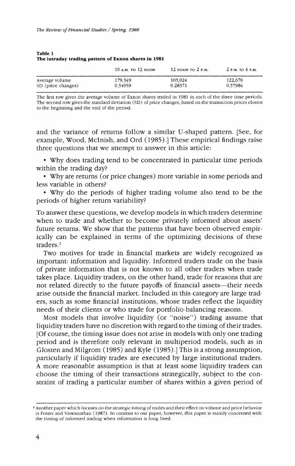
Consider, for example, the data in Table 1 concerning shares of Exxon traded during 1981.1 The U-shaped pattern of the average volume of shares traded-namely, the heavy trading in the beginning and the end of the trading day and the relatively light trading in the middle of the day-is very typical and has been documented in a number of studies. [For example,Jain andJoh (1986) examine hourly data for the aggregate volume on the NYSE, which is reported in the Wall StreetJournal, and find the same pattern.] Both the variance of price changes
We would like to thank Michihiro Kandori, Allan Kleidon, David Kreps, Pete Kyle, Myron Scholes, Ken Singleton, Mark Wolfson, a referee, and especially Mike Gibbons and Chester Spatt for helpful suggestions and comments. We are also grateful to Douglas Foster and S. Viswanathan for pointing out an error in a previous draft. Kobi Boudoukh and Matt Richardson provided valuable research assistance. The financial support of the Stanford Program in Finance aind Batterymarch Financial Management is gratefully acknowledged. Address reprint requests to Anat Admati, Stanford University, Graduate School of Busi- ness, Stanford, CA 94305.
lWe have looked at data for companies in the Dow Jones 30, and the patterns are similar. The transaction data were obtained from Francis Emory Fitch, Inc. We chose Exxon here since it is the most heavily traded stock in the sample.
The Review of Financial Studies 1988, Volume 1, number 1, pp. 3-40. ? 1988 The Review of Financial Studies 0021-9398/88/5904-013 $1.50
3
The Review of Financial Studies / Spring, 1988
Table 1 The intraday trading pattern of Exxon shares in 1981
10 A.M. TO 12 NOON 12 NOON TO 2 P.M. 2 P.M. to 4 P.M.
Average volume 179,349 103,024 122,670 SD (price changes) 0.34959 0.28371 0.37984
The first row gives the average volume of Exxon shares traded in 1981 in each of the three time periods. The second row gives the standard deviation (SD) of price changes, based on the transaction prices closest to the beginning and the end of the period.
and the variance of returns follow a similar U-shaped pattern. [See, for example, Wood, Mclnish, and Ord (1985).] These empirical findings raise three questions that we attempt to answer in this article:
* Why does trading tend to be concentrated in particular time periods within the trading day?
* Why are returns (or price changes) more variable in some periods and less variable in others?
* Why do the periods of higher trading volume also tend to be the periods of higher return variability?
To answer these questions, we develop models in which traders determine when to trade and whether to become privately informed about assets' future returns. We show that the patterns that have been observed empir- ically can be explained in terms of the optimizing decisions of these traders.2
Two motives for trade in financial markets are widely recognized as important: information and liquidity. Informed traders trade on the basis of private information that is not known to all other traders when trade takes place. Liquidity traders, on the other hand, trade for reasons that are not related directly to the future payoffs of financial assets-their needs arise outside the financial market. Included in this category are large trad- ers, such as some financial institutions, whose trades reflect the liquidity needs of their clients or who trade for portfolio-balancing reasons.
Most models that involve liquidity (or "noise") trading assume that liquidity traders have no discretion with regard to the timing of their trades. [Of course, the timing issue does not arise in models with only one trading period and is therefore only relevant in multiperiod models, such as in Glosten and Milgrom (1985) and Kyle (1985).] This is a strong assumption, particularly if liquidity trades are executed by large institutional traders. A more reasonable assumption is that at least some liquidity traders can choose the timing of their transactions strategically, subject to the con- straint of trading a particular number of shares within a given period of
2 Another paper which focuses on the strategic timing of trades and their effect on volume and price behavior is Foster and Viswanathan (1987). In contrast to our paper, however, this paper is mainly concerned with the timing of informed trading when information is long lived.
4
A Theory of Intraday Patterns
time. The models developed in this article include such discretionary liquidity traders, and the actions of these traders play an important role in determining the types of patterns that will be identified. We believe that the inclusion of these traders captures an important element of actual trading in financial markets. We will demonstrate that the behavior of liquidity traders, together with that of potentially informed speculators who may trade on the basis of private information they acquire, can explain some of the empirical observations mentioned above as well as suggest some new testable predictions.
It is intuitive that, to the extent that liquidity traders have discretion over when they trade, they prefer to trade when the market is "thick"-that is, when their trading has little effect on prices. This creates strong incentives for liquidity traders to trade together and for trading to be concentrated. When informed traders can also decide when to collect information and when to trade, the story becomes more complicated. Clearly, informed traders also want to trade when the market is thick. If many informed traders trade at the same time that liquidity traders concentrate their trad- ing, then the terms of trade will reflect the increased level of informed trading as well, and this may conceivably drive out the liquidity traders. It is not clear, therefore, what patterns may actually emerge.
In fact, we show in our model that as long as there is at least one informed trader, the introduction of more informed traders generally intensifies the forces leading to the concentration of trading by discretionary liquidity traders. This is because informed traders compete with each other, and this typically improves the welfare of liquidity traders. We show that li- quidity traders always benefit from more entry by informed traders when informed traders have the same information. However, when the infor- mation of each informed trader is different (i.e., when information is diverse among informed traders), then this may not be true. As more diversely informed traders enter the market, the amount of information that is avail- able to the market as a whole increases, and this may worsen the terms of trade for everyone. Despite this possibility, we show that with diversely informed traders the patterns that generally emerge involve a concentra- tion of trading.
The trading model used in our analysis is in the spirit of Glosten and Milgrom (1985) and especially Kyle (1984, 1985). Informed traders and liquidity traders submit market orders to a market maker who sets prices so that his expected profits are zero given the total order flow. The infor- mation structure in our model is simpler than Kyle (1985) and Glosten and Milgrom (1985) in that private information is only useful for one period. Like Kyle (1984, 1985) and unlike Glosten and Milgrom (1985), orders are not constrained to be of a fixed size such as one share. Indeed, the size of the order is a choice variable for traders.
What distinguishes our analysis from these other papers is that we exam- ine, in a simple dynamic context, the interaction between strategic informed traders and strategic liquidity traders. Specifically, our models include two
5

The Review of Financial Studies / Spring, 1988
types of liquidity traders. Nondiscretionary liquidity traders must trade a particular number of shares at a particular time (for reasons that are not modeled). In addition, we assume that there are some discretionary li- quidity traders, who also have liquidity demands, but who can be strategic in choosing when to execute these trades within a given period of time, e.g., within 24 hours or by the end of the trading day. It is assumed that discretionary liquidity traders time their trades so as to minimize the (expected) cost of their transactions.
Kyle (1984) discusses a single period version of the model we use and derives some comparative statics results that are relevant to our discussion. In his model, there are multiple informed traders who have diverse infor- mation. There are also multiple market makers, so that the model we use is a limit of his model as the number of market makers grows. Kyle (1984) discusses what happens to the informativeness of the price as the variance of liquidity demands changes. He shows that with a fixed number of informed traders the informativeness of the price does not depend on the variance of liquidity demand. However, if information acquisition is endogenous, then price informativeness is increasing in the variance of the liquidity demands. These properties of the single period model play an important role in our analysis, where the variance of liquidity demands in different periods is determined in equilibrium by the decisions of the discretionary liquidity traders.
We begin by analyzing a simple model that involves a fixed number of informed traders, all of whom observe the same information. Discretionary liquidity traders can determine the timing of their trade, but they can trade only once during the time period within which they must satisfy their liquidity demand. (Such a restriction may be motivated by per-trade trans- action costs.) We show that in this model there will be patterns in the volume of trade; namely, trade will tend to be concentrated. If the number and precision of the information of informed traders is constant over time, however, then the information content and variability of equilibrium prices will be constant over time as well.
We then discuss the effects of endogenous information acquisition and of diverse private information. It is assumed that traders can become informed at a cost, and we examine the equilibrium in which no more traders wish to become informed. We show that the patterns of trading volume that exist in the model with a fixed number of informed traders become more pronounced if the number of informed traders is endoge- nous. The increased level of liquidity trading induces more informed trad- ing. Moreover, with endogenous information acquisition we obtain pat- terns in the informativeness of prices and in price variability.
Another layer is added to the model by allowing discretionary liquidity traders to satisfy their liquidity needs by trading more than once if they choose. The trading patterns that emerge in this case are more subtle. This is because the market maker can partially predict the liquidity-trading
6

A Theory of Intraday Patterns
component of the order flow in later periods by observing previous order flows.
This article is organized as follows. In Section 1 we discuss the model with a fixed number of (identically) informed traders. Section 2 considers endogenous information acquisition, and Section 3 extends the results to the case of diversely informed traders. In Section 4 we relax the assumption that discretionary liquidity traders trade only once. Section 5 explores some additional extensions to the model and shows that our results hold in a number of different settings. In Section 6 we discuss some empirically testable predictions of our model, and Section 7 provides concluding remarks.
1. A Simple Model of Trading Patterns
1.1 Model description We consider a single asset traded over a span of time that we divide into T periods. It is assumed that the value of the asset in period T is exoge- nously given by
T
F = F +: at (1) t=l
where &t, t= 1, 2, .. . , T, are independently distributed random variables, each having a mean of zero. The payoff Fcan be thought of as the liquidation value of the asset: any trader holding a share of the asset in period T receives a liquidating dividend of Fdollars. Alternatively, period Tcan be viewed as a period in which all traders have the same information about the value of the asset and F is the common value that each assigns to it. For example, an earnings report may be released in period T. If this report reveals all those quantities about which traders might be privately informed, then all traders will be symmetrically informed in this period.
In periods prior to T, information about Fis revealed through both public and private sources. In each period t the innovation 3, becomes public knowledge. In addition, some traders also have access to private infor- mation, as described below. In subsequent sections of this article we will make the decision to become informed endogenous; in this section we assume that in period t, n, traders are endowed with private information. A privately informed trader observes a signal that is informative about bt+1. Specifically, we assume that an informed trader observes 6t+l + Et, where var(E,) = kt. Thus, privately informed traders observe something about the piece of public information that will be revealed one period later to all traders. Another interpretation of this structure of private information is that privately informed traders are able to process public information faster or more efficiently than others are. (Note that it is assumed here that all informed traders observe the same signal. An alternative formulation is considered in Section 3.) Since the private information becomes useless
7

The Review of Financial Studies/ Spring, 1988
one period after it is observed, informed traders only need to determine their trade in the period in which they are informed. Issues related to the timing of informed trading, which are important in Kyle (1985), do not arise here. We assume throughout this article that in each period there is at least one privately informed trader.
All traders in the model are risk-neutral. (However, as discussed in Section 5.2, our basic results do not change if some traders are risk-averse.) We also assume for simplicity and ease of exposition that there is no discounting by traders.3 Thus, if 4)t summarizes all the information observed by a particular trader in period t, then the value of a share of the asset to that trader in period t is E(FI 4t), where EQ K ) is the conditional expec- tation operator.
In this section we are mainly concerned with the behavior of the liquidity traders and its effect on prices and trading volume. We postulate that there are two types of liquidity traders. In each period there exists a group of nondiscretionary liquidity traderswho must trade a given number of shares in that period. The other class of liquidity traders is composed of traders who have liquidity demands that need not be satisfied immediately. We call these discretionary liquidity traders and assume that their demand for shares is determined in some period T' and needs to be satisfied before period T", where T' < T" < T. Assume there are m discretionary liquidity traders and let Y' be the total demand of the jth discretionary liquidity trader (revealed to that trader in period T'). Since each discretionary li- quidity trader is risk-neutral, he determines his trading policy so as to minimize his expected cost of trading, subject to the condition that he trades a total of Y' shares by period T". Until Section 4 we assume that each discretionary liquidity trader only trades once between time T' and time T"; that is, a liquidity trader cannot divide his trades among different periods.
Prices for the asset are established in each period by a market maker who stands prepared to take a position in the asset to balance the total demand of the remainder of the market. The market maker is also assumed to be risk-neutral, and competition forces him to set prices so that he earns zero expected profits in each period. This follows the approach in Kyle (1985) and in Glosten and Milgrom (1985).5
3This assumption is reasonable since the span of time covered by the Tperiods in this model is to be taken as relatively short and since our main interests concern the volume of trading and the variability of prices. The nature of our results does not change if a positive discount rate is assumed.
4In reality, of course, different traders may realize their liquidity demands at different times, and the time that caln elapse before these demands must be satisfied may also be different for different traders. The nature of our results will not change if the model is complicated to capture this. See the discussion in Section 5.1.
5The model here can be viewed as the limit of a model with a finite number of market makers as the number of market makers grows to infinity. However, our results do not depend in any important way on the assumption of perfect competition among market makers. The same basic results would obtain in an analogous model with a finite number of market makers, where each market maker announces a (linear) pricing schedule as a function of his own order flow and traders can allocate their trade among different market makers. In such a model, market makers earn positive expected profits. See Kyle (1984).
8

A Theory of Intraday Patterns
Let x/ be the ith informed trader's order in period t, 5/ be the order of the jth discretionary liquidity trader in that period, and let us denote by Zt the total demand for shares by the nondiscretionary liquidity traders in period t. Then the market maker must purchase )t = 2t=, Jti + 2yj=l 5! + it shares in period t. The market maker determines a price in period t based on the history of public information, 6,, 62. , bt, and on the history of order flows, ul, 72, . . , Ut 6 Let At = (&1, * *t) and let Qt = ('1 w2,
* I * X &0). The zero expected profit condition implies that Pt, the price set in period t by the market maker, satisfies
Pt = E(FI A-t, Qt) (2)
Finally, we assume that the random variables
I., I, * * , Z1, 2, * *X T-1X 61, 62X * 6T, El, E2 ***XET-1)
are mutually independent and distributed multivariate normal, with each variable having a mean of zero.
1.2 Equilibrium We will be concerned with the (Nash) equilibria of the trading game that our model defines among traders. Under our assumptions, the market maker has a passive role in the model.7 Two types of traders do make strategic decisions in our model. Informed traders must determine the size of their market order in each period. At time t, this decision is made knowing Qt-lx the history of order flows up to period t - 1; At, the inno- vations up to t; and the signal, t+l + et. The discretionary liquidity traders must choose a period in [T', T"] in which to trade. Each trader takes the strategies of all other traders, as well as the terms of trade (summarized by the market maker's price-setting strategy), as given.
The market maker, who only observes the total order flow, sets prices to satisfy the zero expected profit condition. We assume that the market maker's pricing response is a linear function of Qt and At. In the equilibrium that emerges, this will be consistent with the zero-profit condition. Given our assumptions, the market maker learns nothing in period t from past order flows (Qt-l) that cannot be inferred from the public information At. This is because past trades of the informed traders are independent of bt+l,
bt+2,... , bTand because the liquidity trading in any period is independent of that in any other period. This means that the price set in period t is equal to the expectation of Fconditional on all public information observed in that period plus an adjustment that reflects the information contained in the current order flow t:
' If the price were a function of individual orders, then anonymous traders could manipulate the price by submitting canceling orders. For example, a trader who wishes to purchase 10 shares could submit a purchase order for 200 shares and a sell order for 190 shares. When the price is solely a function of the total order flow, such manipulations are not possible.
I It is actually possible to think of the market maker also as a player in the game, whose payoff is minus the sum of the squared deviations of the prices from the true payoff.
9
The Review of Financial Studies/ Spring, 1988
Pt(At I Xt) = E(FI At) + Xt4t
= F + : + x ta t (3) T=1
Our notation conforms with that in Kyle (1984, 1985). The reciprocal of Xt is Kyle's market-depth parameter, and it plays an important role in our analysis.
The main result of this section shows that in equilibrium there is a tendency for trading to be concentrated in the same period. Specifically, we will show that equilibria where all discretionary liquidity traders trade in the same period always exist and that only such equilibria are robust to slight changes in the parameters.
Our analysis begins with a few simple results that characterize the equi- libria of the model. Suppose that the total amount of discretionary liquidity demands in period t is j 5/, where yj = Yiif the jth discretionary liquidity trader trades in period t and where 5/= 0 otherwise. Define *tI
var(Zj1l Yj + Z~t); that is, It is the total variance of the liquidity trading in period t. (Note that 'Pt must be determined in equilibrium since it depends on the trading positions of the discretionary liquidity traders.) The follow- ing lemma is proved in the Appendix.
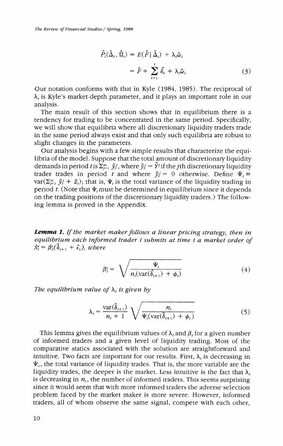
Lemma 1. If the market maker follows a linear pricing strategy, then in equilibrium each informed trader i submits at time t a market order of kti= Ot(?t+l + (t, where
I *t t nt(var(Qt+3) + ot) (4)
The equilibrium value of Xt is given by
_ var(bt+l) / _nt_(5)
nt + 1 V+t(var(6t+1) + kt)
This lemma gives the equilibrium values of Xt and Ot for a given number of informed traders and a given level of liquidity trading. Most of the comparative statics associated with the solution are straightforward and intuitive. Two facts are important for our results. First, Xt is decreasing in 't, the total variance of liquidity trades. That is, the more variable are the
liquidity trades, the deeper is the market. Less intuitive is the fact that Xt is decreasing in nt, the number of informed traders. This seems surprising since it would seem that with more informed traders the adverse selection problem faced by the market maker is more severe. However, informed traders, all of whom observe the same signal, compete with each other,
10
A Theory of Intraday Patterns
and this leads to a smaller Xt. This is a key observation in the next section, where we introduce endogenous entry by informed traders.8
When some of the liquidity trading is discretionary, Jt is an endogenous parameter. In equilibrium each discretionary liquidity trader follows the trading policy that minimizes his expected transaction costs, subject to meeting his liquidity demand Y' We now turn to the determination of this equilibrium behavior. Recall that each trader takes the value of Xt (as well as the actions of other traders) as given and assumes that he cannot influ- ence it. The cost of trading is measured as the difference between what the liquidity trader pays for the security and the security's expected value. Specifically, the expected cost to the jth liquidity trader of trading at time t E [ T', T"] is
E((Pt( t, 7t) - F)YitA7Q- YJ)(
Substituting for Pt(At, Qt)-and using the fact that Zt 7 i=i j and 6, where = t + 1, t + 2, ... Tare independent of At, Qt-, and Y} (which is the
information of discretionaryliquiditytraderj)-the cost simplifies toX y ) 2.
Thus, for a given set of Xt, tE[ T', T"], the expected cost of liquidity trading is minimized by trading in that period t* E [T', T"] in which Xt is the smallest. This is very intuitive, since Xt measures the effect of each unit of order flow on the price and, by assumption, liquidity traders trade only once.
Recall that from Lemma 1, Xt is decreasing in Lt. This means that if in equilibrium the discretionary liquidity trading is particularly heavy in a particular period t, then Xt will be set lower, which in turn makes discre- tionary liquidity traders concentrate their trading in that period. In sum, we obtain the following result.
Proposition 1. There always exist equilibria in which all discretionary liquidity trading occurs in the same period. Moreover, only these equilibria are robust in the sense that iffor some set of parameters there exists an equilibrium in which discretionary liquidity traders do not trade in the same period, then for an arbitrarily close set of parameters (e.g., by per- turbing the vector of variances of the liquidity demands Yi), the only possible equilibria involve concentrated trading by the discretionary li- quidity traders.
More intuition for why X, is decreasing in n, can be otained from statistical inference. Recall that X, is the regression coefficient in the forecast of 6,,,, given the total order flow j,. The order flow can be written as a(b,+, + c,) + ui, where a(b,+1 + c,) represents the total trading position of the informed traders and it is the position of the liquidity traders with var(ii) = T. As the number of informed traders increases, a increases. For a given level of a, the market maker sets X, equal to X(a) = a/(a2(1 + 4) + 'I). This is an increasing function of a if and only if a < 'P1(1 + 4 which in this model occurs if and only if n, - 1, We can think of the market maker's inference problem in two parts: first he uses co, to predict ab,; then he scales this down by a factor of 1/a to obtain his prediction of 6,. The weight placed upon ), in predicting ab,+, is always increasing in a, but for a large enough value of a the scaling down by a factor of 1/a eventually dominates, lowering X,.
The Review of Financial Studies/ Spring, 1988
Proof Define h var(N?21 i), that is, the total variance of discretionary liquidity demands. Suppose that all discretionary liquidity traders trade in period t and that the market maker adjusts Xt and informed traders set ft accordingly. Then the total trading cost incurred by the discretionary trad- ers is Xt(h) h, where Xt(h) is given in Lemma 1 with It = h + var(it).
Consider the period t* E [T', T"] for which Xt(h) is the smallest. (If there are several periods in which the smallest value is achieved, choose the first.) It is then an equilibrium for all discretionary traders to trade in t*. This follows since Xt(h) is decreasing in h, so that we must have by the definition of t*, Xt(O) >- Xt(h) for all t E [T', T"]. Thus, discretionary liquidity traders prefer to trade in period t*.
The above argument shows that there exist equilibria in which all dis- cretionary liquidity trading is concentrated in one period. If there is an equilibrium in which trading is not concentrated, then the smallest value of Xt must be attained in at least two periods. It is easy to see that any small change in var( Yi) for somejwould make the X, different in different periods, upsetting the equilibrium. U
Proposition 1 states that concentrated-trading patterns are always viable and that they are generically the only possible equilibria (given that the market maker uses a linear strategy). Note that in our model all traders take the values of Xt as given. That is, when a trader considers deviating from the equilibrium strategy, he assumes that the trading strategies of other traders and the pricing strategy of the market maker (i.e., Xt) do not change.9 One may assume instead that liquidity traders first announce the timing of their trading and then trading takes place (anonymously), so that informed traders and the market maker can adjust their strategies according to the announced timing of liquidity trades. In this case the only possible equilibria are those where trading is concentrated. This follows because if trading is not concentrated, then some liquidity traders can benefit by deviating and trading in another period, which would lower the value of Xt in that period.
We now illustrate Proposition 1 by an example. This example will be used and developed further in the remainder of this article.
Example. Assume that T = 5 and that discretionary liquidity traders learn of their demands in period 2 and must trade in or before period 4 (i.e., T' = 2 and T" = 4). In each of the first four periods, three informed traders trade, and we assume that each has perfect information. Thus, each observes in period tthe realization of bt+. We assume that public information arrives at a constant rate, with var(St) = 1 for all t. Finally, the variance of the nondiscretionary liquidity trading occurring each period is set equal to 1.
9 Interestingly, when n, = 1 the equilibrium is the same whether the informed trader takes Xt as given or whether he takes into account the effect his trading policy has on the market maker's determination of X,. In other words, in this model the Nash equilibrium in the game between the informed trader and the market maker is identical to the Stackelberg equilibrium in which the trader takes the market maker's response into account.
12

A Theory of Intraday Patterns
We are interested in the behavior of the discretionary liquidity traders. Assume that there are two of these traders, A and B, and let var(YA) = 4 and var(YB) = 1. First assume that A trades in period 2 and B trades in period 3. Then X1 = X4 = 0.4330, X2 = 0.1936 and X3 = 0.3061. This cannot be an equilibrium, since X2 < X3, so B will want to trade in period 2 rather than in period 3. The discretionary liquidity traders take the X's as fixed and B perceives that his trading costs can be reduced if he trades earlier. Now assume that both discretionary liquidity traders trade in period 3. In this case Al = A2 = X4 = 0.4330 and A3 = 0.1767. This is clearly a stable trading pattern. Both traders want to trade in period 3 since A3 is the minimal Xt.
1.3 Implications for volume and price behavior In this section we show that the concentration of trading that results when some liquidity traders choose the timing of their trades has a pronounced effect on the volume of trading. Specifically, the volume is higher in the period in which trading is concentrated both because of the increased liquidity-trading volume and because of the induced informed-trading vol- ume. The concentration of discretionary liquidity traders does not affect the amount of information revealed by prices or the variance of price changes, however, as long as the number of informed traders is held fixed and is specified exogenously. As we show in the next section, the results on price informativeness and on the variance of price changes are altered if the number of informed traders in the market is determined endoge- nously.
It is clear that the behavior of prices and of trading volume is determined in part by the rate of public-information release and the magnitude of the nondiscretionary liquidity trading in each period. Various patterns can easily be obtained by making the appropriate assumptions about these exogenous variables. Since our main interest in this article is to examine the effects of traders' strategic behavior on prices and volume, we wish to abstract from these other determinants. If the rate at which information becomes public is constant and the magnitude of nondiscretionary liquid- ity trading is the same in all periods, then any patterns that emerge are due solely to the strategic behavior of traders. We therefore assume in this section that var(- ) = g, var(&t) = 1, and var(E,) = + for all t. Setting var(b5) to be constant over time guarantees that public information arrives at a constant rate. [The normalization of var(bt) to 1 is without loss of gener- ality.]
Before presenting our results on the behavior of prices and trading volume, it is important to discuss how volume should be measured. Sup- pose that there are k traders with market orders given by .-, -2,.. .,
Assume that the 52 are independently and normally distributed, each with mean 0. Let 9j+ = max(Q., 0) and s- = max(-9j, 0). The total volume of trade (including trades that are "crossed" between traders) is max(S+, S-), where S+ = .9t+ and S- = =1 s-k . The expected volume is
13
The Review of Financial Studies / Spring, 1988
1 k 1 k
E(max(S+, S-) - 2 El sjj + - E K i 2 _ ' 2
(k k
\/ i + \ 0 $) (7)
where vi is the standard deviation of 9,. One may think that var(cot), the variance of the total order flow, is appro-
priate for measuring the expected volume of trading. This is not correct. Since &Ut is the net demand presented to the market maker, it does not include trades that are crossed between traders and are therefore not met by the market maker. For example, suppose that there are two traders in period t and that their market orders are 10 and -16, respectively (i.e., the first trader wants to purchase 10 shares, and the second trader wants to sell 16 shares). Then the total amount of trading in this period is 16 shares, 10 crossed between the two traders and 6 supplied by the market maker (Cot = 6 in this case). The parameter var(wt), which is represented by the last term in Equation (7), only considers the trading done with the market maker. The other terms measure the expected volume of trade across traders. In light of the above discussion, we will focus on the fol- lowing measures of trading volume, which identify the contribution of each group of traders to the total trading volume:
V,' var( n,ft(6t+l + c')) (8)
m VtL - + var(i) (9)
j =1
VM var(') (10)
vt -Vt + Vt/ + vt (1 1)
In words, VtIand Vt1 measure the expected volume of trading of the informed traders and the liquidity traders, respectively, and VtM measures the expected trading done by the market maker. The total expected volume, Vt, is the sum of the individual components. These measures are closely related to the true expectation of the actual measured volume.10
Proposition 1 asserts that a typical equilibrium for our model involves the concentration of all discretionary liquidity trading in one period. Let
10 Our measure of volume is proportional to the actual expected volume if there is exactly one nondiscre- tionary liquidity trader; otherwise, the trading crossed between these traders will not be counted, and V,7 will be lower than the true contribution of the liquidity traders. This presents no problem for our analysis, however, since the amount of this trading in any period is independent of the strategic behavior of the other traders.
14

A Theory of Intraday Patterns
this period be denoted by t*. Note that if we assume that nt, var(at), var(ke), and var(i;) are independent of t, then t* can be any period in [T',
TJ. The following result summarizes the equilibrium patterns of trading
volume in our model.
Proposition 2. In an equilibrium in which all discretionary liquidity trading occurs in period t*>
1. Vt/ > Vtfort t*
2. VF A> VtI for t t*
3. V> Vmfort# t*
Proof Part 1 is trivial, since there is more liquidity trading in t* than in other periods. To prove part 2, note that
VI= Vvar(ntIt(6t+, + c) =) (12)
Thus, an increase in *tI the total variance of liquidity trading, decreases Xt and increases the informed component of trading. Part 3 follows imme- diately from parts 1 and 2. U
This result shows that the concentration of liquidity trading increases the volume in the period in which it occurs not only directly through the actual liquidity trading (an increase in V>) but also indirectly through the additional informed trading it induces (an increase in Vt/). This is an example of trading generating trading. An example that illustrates this phenomenon is presented following the next result."
We now turn to examine two endogenous parameters related to the price process. The first parameter measures the extent to which prices reveal private information, and it is defined by
Qt var(t&+ P1) (13)
The second is simply the variance of the price change:
Rt- var(P - Pt-,) (14)
Proposition 3. Assume that n, = n for every t. Then
1. Qt. =Qtfor every t 2. Rt.Rt =1 for every t
Proof It is straightforward to show that in general
Qt ( 1 + n nt4) (15)
Note that the amount of informed trading is independent of the precision of the signal that informed traders observe. This is due to the assumed risk neutrality of informed traders.
15

The Review of Financial Studies / Spring, 1988
and Rt 1 n + +?,) (16)
The result follows since both Rt and Q, are independent of It, and nt = n. m
As observed in Kyle (1984, 1985), the amount of private information revealed by the price is independent of the total variance of liquidity trading. Thus, despite the concentration of trading in t*, Qt. = Qt for all t. The intuition behind this is that although there is more liquidity trading in period t*, there is also more informed trading, as we saw in Proposition 2. The additional informed trading is just sufficient to keep the information content of the total order flow constant.
Proposition 3 also says that the variance of price changes is the same when n informed traders trade in each period as it is when there is no informed trading. [When there is no informed trading, Ft,- Pt-, = bt, so Rt= var(6t) = 1 for all t.] With some informed traders, the market gets information earlier than it would otherwise, but the overall rate at which information comes to the market is unchanged. Moreover, the variance of price changes is independent of the variance of liquidity trading in period t. As will be shown in the next section, these results change if the number of informed traders is determined endogenously. Before turning to this analysis, we illustrate the results of this section with an example.
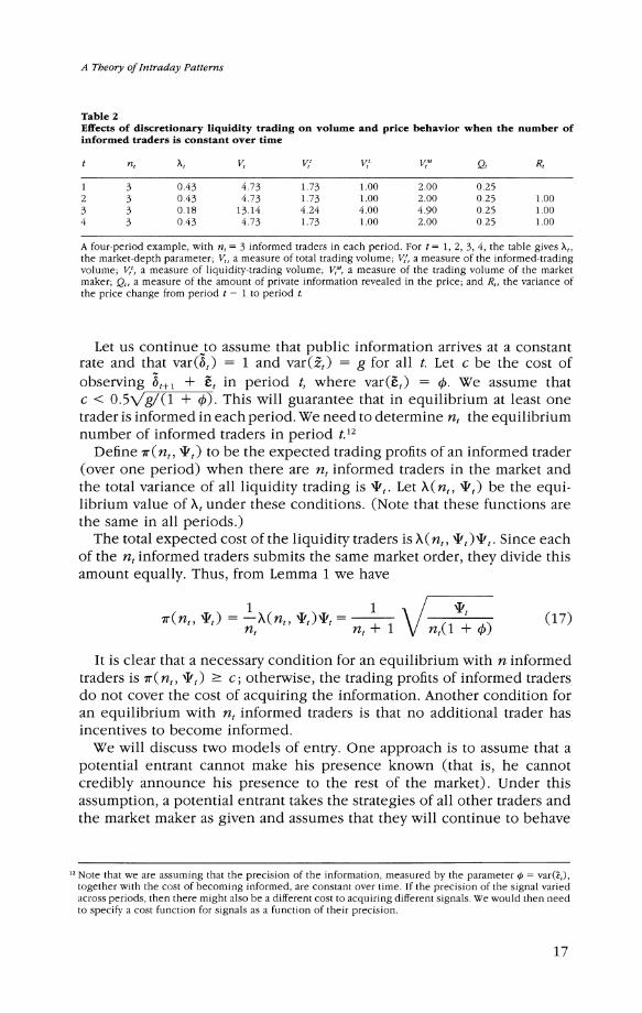
Example (continued). Consider again the example introduced in Section 1.2. Recall that in the equilibrium we discussed, both of the discretionary liquidity traders trade in period 3. Table 2 shows the effects of this trading on volume and price behavior. The volume-of-trading measure in period 3 is V3 = 13.14, while that in the other periods is only 4.73. The difference is only partly due to the actual trading of the liquidity traders. Increased trading by the three informed traders in period 3 also contributes to higher volume. As the table shows, both Qt and R, are unaffected by the increased liquidity trading. With three informed traders, three quarters of the private information is revealed through prices no matter what the magnitude of liquidity demand.
2. Endogenous Information Acquisition
In Section 1 the number of informed traders in each period was taken as fixed. We now assume, instead, that private information is acquired at some cost in each period and that traders acquire this information if and only if their expected profit exceeds this cost. The number of informed traders is therefore determined as part of the equilibrium. It will be shown that endogenous information acquisition intensifies the result that trading is concentrated in equilibrium and that it alters the results on the distribution and informativeness of prices.
16
A Theory of Intraday Patterns
Table 2 Effects of discretionary liquidity trading on volume and price behavior when the number of informed traders is constant over time
t n, A, VI V,' VL VIM Q, R,
1 3 0.43 4.73 1.73 1.00 2.00 0.25 2 3 0.43 4.73 1.73 1.00 2.00 0.25 1.00 3 3 0.18 13.14 4.24 4.00 4.90 0.25 1.00 4 3 0.43 4.73 1.73 1.00 2.00 0.25 1.00
A four-period example, with n, = 3 informed traders in each period. For t = 1, 2, 3, 4, the table gives X,, the market-depth parameter; V,, a measure of total trading volume; V,', a measure of the informed-trading volume; V7L, a measure of liquidity-trading volume; V,M, a measure of the trading volume of the market inaker; Q,, a measure of the amount of private information revealed in the price; and R,, the variance of the price change from period t - 1 to period t.
Let us continue to assume that public information arrives at a constant rate and that var(kt) = 1 and var(zt) = g for all t. Let c be the cost of observing &t+j + et in period t, where var(Et) = 0. We assume that c < 0.5Vg/(1 + k). This will guarantee that in equilibrium at least one trader is informed in each period. We need to determine nt the equilibrium number of informed traders in period t.12
Define ir(nt, It) to be the expected trading profits of an informed trader (over one period) when there are nt informed traders in the market and the total variance of all liquidity trading is 'It. Let X(nt, 'It) be the equi- librium value of Xt under these conditions. (Note that these functions are the same in all periods.)
The total expected cost of the liquidity traders is X(nt, I't)It. Since each of the nt informed traders submits the same market order, they divide this amount equally. Thus, from Lemma 1 we have
1 _ _ _ _ _ _ _ _ _ _ _ _
ir(nt, TtI) =-X(nt, t)t = +1 ( 17) nt ~~nt+ 1 nt(1 0) (7
It is clear that a necessary condition for an equilibrium with n informed traders is r(nt, It) > C; otherwise, the trading profits of informed traders do not cover the cost of acquiring the information. Another condition for an equilibrium with nt informed traders is that no additional trader has incentives to become informed.
We will discuss two models of entry. One approach is to assume that a potential entrant cannot make his presence known (that is, he cannot credibly announce his presence to the rest of the market). Under this assumption, a potential entrant takes the strategies of all other traders and the market maker as given and assumes that they will continue to behave
12 Note that we are assuming that the precision of the information, measured by the parametero = var(e,), together with the cost of becoming informed, are constant over time. If the precision of the signal varied across periods, then there might also be a different cost to acquiring different signals. We would then need to specify a cost function for signals as a function of their precision.
17

The Review of Financial Studies / Spring, 1988
Table 3 Expected trading profits of informed traders when the variance of liquidity demand is 6
n r(n, 6) V4r(n, 6)
1 1.225 0.306 2 0.577 0.144 3 0.354 0.088 4 0.245 0.061 5 0.183 0.046 6 0.143 0.038 7 0.116 0.029
For some possible number of informed traders, n, the table gives ir(n, 6), the expected profits of each of the informed traders, assuming that the variance of total liquidity trading is 6; and ir(n, 6)/4, the profits of an entrant who assumes that all other traders will use the same equilibrium strategies after he enters as an informed trader. If the cost of information is 0.13, then the equilibrium number of informed traders is n e {3, 4, 5, 6} in the first approach and n = 6 in the second.
as if n, traders are informed. Thus we still have X = X(nt, XI'). The following lemma gives the optimal market order for an entrant and his expected trading profits under this assumption. (The proof is in the Appendix.)
Lemma 2. An entrant into a market with n, informed traders will trade exactly half the number of shares as the other n, traders for any realization of the signal, and his expected profits will be ir(nt, *t)/4.
It follows that with this approach nt is an equilibrium number of informed traders in period t if and only if n, satisfies ir(nt, 't)/4 < c < 7r(nt, It). If c is large enough, there may be no positive integer nt satisfying this condition, so that the only equilibrium number of informed traders is zero. However, the assumption that c < 0.5\/g/(1 + O) guarantees that this is never the case. In general, there may be several values of nt that are consistent with equilibrium according to this model.
An alternative model of entry by informed traders is to assume that if an additional trader becomes informed, other traders and the market maker change their strategies so that a new equilibrium, with n, + 1 informed traders, is reached. If liquidity traders do not change their behavior, the profits of each informed trader would now become ir(nt + 1, 't).13 The largest ntsatisfying ir(nt, 't))/4 < c ?< r(nt, 't) is the (unique) n satisfying ir(nt + 1, *t) < c -< r(nt, It), which is the condition for equilibrium under the alternative approach. This is illustrated in the example below.
Example (continued). Consider again the example introduced in Section 1.2 (and developed further in Section 1.3). In period 3, when both of the discretionary liquidity traders trade, the total variance of liquidity trading iS 3 = 6. Assume that the cost of perfect information is c = 0.13. Table 3 gives ir(n, 6) and ir(n, 6)/ as a function of some possible values for n.
13 In fact, the same equilibrium obtains if liquidity traders were assumed to respond to the entry of an informrled trader, as will be clear below.
18
A Theory of Intraday Patterns
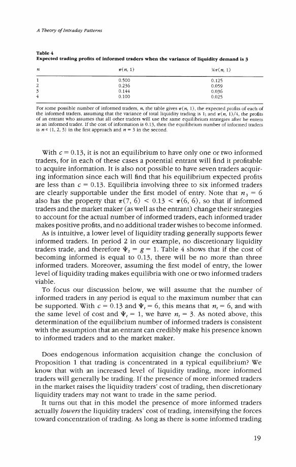
Table 4 Expected trading profits of informed traders when the variance of liquidity demand is 3
n r(n, 1) Vir(n, 1)
1 0.500 0.125 2 0.236 0.059 3 0.144 0.036 4 0.100 0.025
For some possible number of informed traders, n, the table gives ir(n, 1), the expected profits of each of the informed traders, assuming that the variance of total liquidity trading is 1; and r(n, 1)/4, the profits of an entrant who assumes that all other traders will use the same equilibrium strategies after he enters as an informed trader. If the cost of information is 0.13, then the equilibrium number of informed traders is n E {1, 2, 3} in the first approach and n = 3 in the second.
With c = 0.13, it is not an equilibrium to have only one or two informed traders, for in each of these cases a potential entrant will find it profitable to acquire information. It is also not possible to have seven traders acquir- ing information since each will find that his equilibrium expected profits are less than c = 0.13. Equilibria involving three to six informed traders are clearly supportable under the first model of entry. Note that n3 = 6 also has the property that ir(7, 6) < 0.13 < ir(6, 6), so that if informed traders and the market maker (as well as the entrant) change their strategies to account for the actual number of informed traders, each informed trader makes positive profits, and no additional trader wishes to become informed.
As is intuitive, a lower level of liquidity trading generally supports fewer informed traders. In period 2 in our example, no discretionary liquidity traders trade, and therefore T2 = g = 1. Table 4 shows that if the cost of becoming informed is equal to 0.13, there will be no more than three informed traders. Moreover, assuming the first model of entry, the lower level of liquidity trading makes equilibria with one or two informed traders viable.
To focus our discussion below, we will assume that the number of informed traders in any period is equal to the maximum number that can be supported. With c = 0.13 and T, = 6, this means that n, = 6, and with the same level of cost and TI = 1, we have n, = 3. As noted above, this determination of the equilibrium number of informed traders is consistent with the assumption that an entrant can credibly make his presence known to informed traders and to the market maker.
Does endogenous information acquisition change the conclusion of Proposition 1 that trading is concentrated in a typical equilibrium? We know that with an increased level of liquidity trading, more informed traders will generally be trading. If the presence of more informed traders in the market raises the liquidity traders' cost of trading, then discretionary liquidity traders may not want to trade in the same period.
It turns out that in this model the presence of more informed traders actually lowers the liquidity traders' cost of trading, intensifying the forces toward concentration of trading. As long as there is some informed trading
19
The Review of Financial Studies / Spring, 1988
in every period, liquidity traders prefer that there are more rather than fewer informed traders trading along with them. Of course, the best situ- ation for liquidity traders is for there to be no informed traders, but for nt > 0, the cost of trading is a decreasing function of nt. The total cost of trading for the liquidity traders was shown to be X(nt, Jt)'t. That this cost is decreasing in n follows from the fact that X(nt, 't) is decreasing in nt.
Thus, endogenous information acquisition intensifies the effects that bring about the concentration of trading. With more liquidity trading in a given period, more informed traders trade, and this makes it even more attractive for liquidity traders to trade in that period. As already noted, the intuition behind this result is that competition among the privately informed traders reduces their total profit, which benefits the liquidity traders.
The following proposition describes the effect of endogenous infor- mation acquisition on the trading volume and price process.14
Proposition 4. Suppose that the number of informed traders in period t is the unique nt satisfying ir( nt + 1, 'J't) < c : 1r(nt, 3 t) (i.e., determined by the second model of entry). Consider an equilibrium in which all discretionary liquidity traders trade in period t*. Then
1. Vt. > Vt for t :#t
2. VtI. > VtI fort=# t *
3. Qt < Qt for t t r 4. Rt* > Rt*-, > Rt*+,
Proof. The first three statements follow simply from the fact that Vt and VI are increasing in nt, and that Qt is decreasing in nt. The last follows from Equation (16). M
Example (continued). We consider again our example, but now with endogenous information acquisition. Suppose that the cost of acquiring perfect information is 0.13. In periods 1, 2, and 4, when no discretionary liquidity traders trade, there will continue to be three informed traders trading, as seen in Table 4. In period 3, when both of the discretionary liquidity traders trade, the number of informed traders will now be 6, as seen in Table 3. Table 5 shows what occurs with the increased number of informed traders in period 3.
With the higher number of informed traders, the value of X3 is reduced even further, to the benefit of the liquidity traders. It is therefore still an equilibrium for the two discretionary liquidity traders to trade in period 3. Because three more informed traders are present in the market in this period, the total trading cost of the liquidity traders (discretionary and nondiscretionary) is reduced by 0.204, or 19 percent.
14 A cormparative statics result analogous to part 3 is discussed in Kyle (1984).
20
A Theory of Intraday Patterns
Table 5 Effects of discretionary liquidity trading on volume and price behavior when the number of informed traders is endogenous
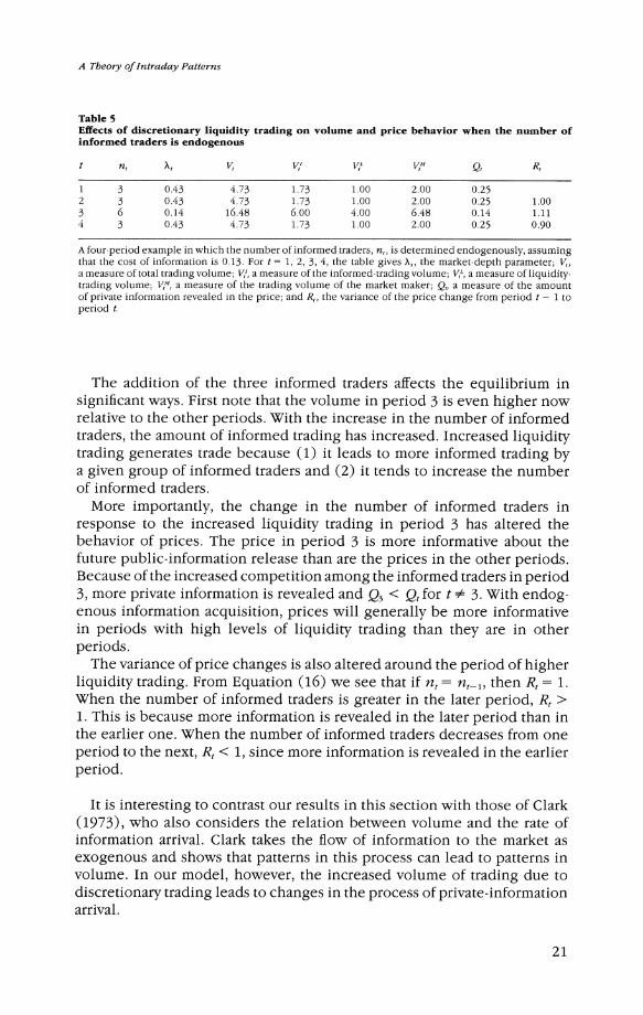
t n, X, VI V,' V, VIM Q, R,
1 3 0.43 4.73 1.73 1.00 2.00 0.25 2 3 0.43 4.73 1.73 1.00 2.00 0.25 1.00 3 6 0.14 16.48 6.00 4.00 6.48 0.14 1.11 4 3 0.43 4.73 1.73 1.00 2.00 0.25 0.90
A four-period example in which the number of informed traders, n, is determined endogenously, assuming that the cost of information is 0.13. For t = 1, 2, 3, 4, the table gives X,, the market-depth parameter; V, a measure of total trading volume; V,', a measure of the informed-trading volume; V,L, a measure of liquidity- trading volume; V,M, a measure of the trading volume of the market maker; Q,, a measure of the amount of private information revealed in the price; and R,, the variance of the price change from period t - 1 to period t.
The addition of the three informed traders affects the equilibrium in significant ways. First note that the volume in period 3 is even higher now relative to the other periods. With the increase in the number of informed traders, the amount of informed trading has increased. Increased liquidity trading generates trade because (1) it leads to more informed trading by a given group of informed traders and (2) it tends to increase the number of informed traders.
More importantly, the change in the number of informed traders in response to the increased liquidity trading in period 3 has altered the behavior of prices. The price in period 3 is more informative about the future public-information release than are the prices in the other periods. Because of the increased competition among the informed traders in period 3, more private information is revealed and Q3 < Qt for t =# 3. With endog- enous information acquisition, prices will generally be more informative in periods with high levels of liquidity trading than they are in other periods.
The variance of price changes is also altered around the period of higher liquidity trading. From Equation (16) we see that if nt = nt-1, then Rt = 1. When the number of informed traders is greater in the later period, Rt > 1. This is because more information is revealed in the later period than in the earlier one. When the number of informed traders decreases from one period to the next, Rt < 1, since more information is revealed in the earlier period.
It is interesting to contrast our results in this section with those of Clark (1973), who also considers the relation between volume and the rate of information arrival. Clark takes the flow of information to the market as exogenous and shows that patterns in this process can lead to patterns in volume. In our model, however, the increased volume of trading due to discretionary trading leads to changes in the process of private-information arrival.
21
The Review of Financial Studies/ Spring, 1988
3. A Model with Diverse Information
So far we have assumed that all the informed traders observe the same piece of information. In this section we discuss an alternative formulation of the model, in which informed traders observe different signals as in Kyle [1984]. The basic results about trading and volume patterns or price behavior do not change. However, the analysis of endogenous information acquisition is somewhat different.
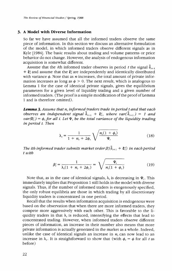
Assume that the ith informed trader observes in period t the signal 6t+? + i and assume that the Ei are independently and identically distributed with variance 0. Note that as n increases, the total amount of private infor- mation increases as long as 0 > 0. The next result, which is analogous to Lemma 1 for the case of identical private signals, gives the equilibrium parameters for a given level of liquidity trading and a given number of informed traders. (The proof is a simple modification of the proof of Lemma 1 and is therefore omitted).
Lemma 3. Assume that nt informed traders trade in period t and that each observes an independent signal 6 + gi, where var(6t+l) = 1 and var(eit) = qt for all i. Let Jt be the total variance of the liquidity trading in period t. Then
A 1 nt(1 + (18)
The ith informed trader submits market order 3i(Qt+l + ;ti) in each period t with
Xt A(1 + nt + 20t) nt(1 + t)9)
Note that, as in the case of identical signals, X, is decreasing in ''. This immediately implies that Proposition 1 still holds in the model with diverse signals. Thus, if the number of informed traders is exogenously specified, the only robust equilibria are those in which trading by all discretionary liquidity traders is concentrated in one period.
Recall that the results when information acquisition is endogenous were based on the observation that when there are more informed traders, they compete more aggressively with each other. This is favorable to the li- quidity traders in that Xt is reduced, intensifying the effects that lead to concentrated trading. However, when informed traders observe different pieces of information, an increase in their number also means that more private information is actually generated in the market as a whole. Indeed, unlike the case of identical signals an increase in nt can now lead to an increase in Xt. It is straightforward to show that (with kt = 0 for all t as before)
22
A Theory of Intraday Patterns
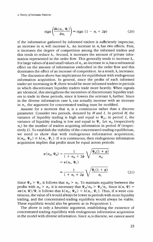
sign (dnt d't) = sign (1 - nt + 20) (20)
If the information gathered by informed traders is sufficiently imprecise, an increase in nt will increase Xt. An increase in nt has two effects. First, it increases the degree of competition among the informed traders and this tends to reduce Xt. Second, it increases the amount of private infor- mation represented in the order flow. This generally tends to increase Xt. For large values of c and small values of nt, an increase in nt has a substantial effect on the amount of information embodied in the order flow and this dominates the effect of an increase of competition. As a result, Xt increases.
The discussion above has implications for equilibrium with endogenous information acquisition. In general, since the profits of each informed trader are increasing in ', there would be more informed traders in periods in which discretionary liquidity traders trade more heavily. When signals are identical, this strengthens the incentives of discretionary liquidity trad- ers to trade in these periods, since it lowers the relevant Xt further. Since in the diverse information case Xt can actually increase with an increase in nt, the argument for concentrated trading must be modified.
Assume for a moment that nt is a continuous rather than a discrete parameter. Consider two periods, denoted by H and L. In period H, the variance of liquidity trading is high and equal to 'IH; in period L, the variance of liquidity trading is low and equal to i"L. Let nH (respectively nL) be the number of traders acquiring information in period H (respec- tively L). To establish the viability of the concentrated-trading equilibrium, we need to show that with endogenous information acquisition, X(nH, "'H) < X(nL, 'IL). If n is continuous, then endogenous information acquisition implies that profits must be equal across periods:
1 *H (1 + f
7r ( nH, *H) =1 + nH+ 2_ nI H
= 7r(nL, "L)
1 nL+ 2 + n (21)
Since PH > >*L, it follows that nH> nL. To maintain equality between the profits with nH> nL it is necessary that *IH/nH > L/fnL- Since X(n, iP) = nr(n, I)/', it follows that X(nH, 'H,) < X(nL, 'IL). Thus, if n were con- tinuous, the value of X would always be lower in periods with more liquidity trading, and the concentrated-trading equilibria would always be viable. These equilibria would also be generic as in Proposition 1.
The above is only a heuristic argument, establishing the existence of concentrated-trading equilibria with endogenous information acquisition in the model with diverse information. Since nt is discrete, we cannot assert
23

The Review of Financial Studies/ Spring 1988
that in equilibrium the profits of informed traders are equal across periods. This may lead to the nonexistence of an equilibrium for some parameter values, as we show in the Appendix. It can be shown, however, that
* An equilibrium always exists if the variance of the discretionary li- quidity demand is sufficiently high.
* If an equilibrium exists, then an equilibrium in which trading is con- centrated exists. Moreover, for almost all parameters for which an equilib- rium exists, only such concentrated-trading equilibria exist.
We now show that, when an equilibrium exists, the basic nature of the results we derived in the previous sections do not change when informed traders have diverse information. We continue to assume that 't = k for all t. Consider first the trading volume. It is easy to show that the variance of the total order flow of the informed traders is given by
/n qft I'(nt + ) var #i3(6t+l + ei (22)
This is clearly increasing in iIit and in nt . Since informed traders are diversely informed, there will generally be some trading within the group of informed traders. (For example, if a particular informed trader draws an extreme signal, his position may have an opposite sign to that of the aggregate position of informed traders.) Thus, VtI, the measure of trading volume by informed traders, will be greater than the expression in Equation (22). The amount of trading within the group of informed traders is clearly an increasing function of nt. Thus, this strengthens the effect of concentrated trading on the volume measures: more liquidity trading leads to more informed traders, which in turn implies an even greater trading volume.
The basic characteristics of the price process are also essentially unchanged in this model. First consider the informativeness of the price, as measured by Q, = var(6,+1 l Pt). With diverse information it can be shown that
Qt 1 + + (23)
As in Kyle (1984), an increase in the number of informed traders increases the informativeness of prices. This is due in part to the increased com- petition among the informed traders. It is also due to the fact that more information is gathered when more traders become informed. This second effect was not present in the model with common private information. The implications of the model remain the same as before: with endogenous information acquisition, prices will be more informative in periods with higher liquidity trading (i.e., periods in which the discretionary liquidity traders trade).
In the model with diverse private information, the behavior of Rt (the variance of price changes) is very similar to what we saw in the model
24

A Theory of Intraday Patterns
with common information. It can be shown that
+t 1+ 20 Rt n +2 1+~+(24) 1t + nt + 20 1 + n, 1 + 2 (24
As before, if nt = n for all t, then Rt = 1, and R, > 1 if and only if nt > nt- i.
4. The Allocation of Liquidity Trading
In the analysis so far we have assumed that the discretionary liquidity traders can only trade once, so that their only decision was the timing of their single trade. We now allow discretionary liquidity traders to allocate their trading among the periods in the interval [T', T"], that is, between the time their liquidity demand is determined and the time by which it must be satisfied. Since the model becomes more complicated, we will illustrate what happens in this case with a simple structure and by numer- ical examples.
Suppose that T' = 1 and T" = 2, so that discretionary liquidity traders can allocate their trades over two trading periods. Suppose that there are n1 informed traders in period 1 and n2 informed traders in period 2 and that the informed traders obtain perfect information (i.e., they observe bt+1 at time t). Each discretionary liquidity trader must choose a, the proportion of the liquidity demand Yi that is satisfied in period 1. The remainder will be satisfied in period 2. Discretionary liquidity trader jtherefore trades a Y shares in period 1 and (1 - a) Yi shares in period 2.
To obtain some intuition, suppose that the price function is as given in the previous sections; that is,
Pt = F +: a + xtcXt (25)
where Xt is given by Lemma 1. Note that the price in period t depends only on the order flow in period t. In this case the discretionary liquidity trader's problem is to minimize the cost of liquidity trading, which is given by
(a2Xi + (1 - a)2X2)(Yj)2 (26)
It is easy to see that this is minimized by setting a = X2/(X1 + X2). For example, if X, = X2, then the optimal value of a is ?2. Thus, if each price is independent of previous order flows, the cost function for a liquidity trader is convex, and so discretionary liquidity traders divide their trades among different periods. It is important to note that the optimal a is inde- pendent of Yi. This means that all liquidity traders will choose the same a.
If the above argument were correct, it would seem to upset our results on the concentration of trade. However, the argument is flawed, since the assumption that each price is independent of past order flows is no longer
25

The Review of Financial Studies/ Spring, 1988
appropriate. Recall that the market maker sets the price in each period equal to the conditional expectation of F, given all the information avail- able to him at the time. This includes the history of past order flows. In the models of the previous sections, there is no payoff-relevant information in past order flows Qt-l that is not revealed by the public information At in period t. This is no longer true here, since past order flows enable the market maker to forecast the liquidity component of current order flows. This improves the precision of his prediction of the informed-trading com- ponent, which is relevant to future payoffs. Specifically, since the infor- mation that informed traders have in period 1 is revealed to the market maker in period 2, the market maker can subtract n431t2 from the total order flow in period 1. This reveals a 2j Y' +
- , which is informative about
(1 - a) j Y', the discretionary liquidity demand in period 2. Since the terms of trade in period 2 depend on the order flow in period
1, a trader who is informed in both periods will take into account the effect that his trading in the first period will have on the profits he can earn in the second period. This complicates the analysis considerably. To avoid these complications and to focus on the behavior of discretionary liquidity traders, we assume that no trader is informed in more than one period.
Suppose that the price in period 1 is given by
PA = P. + bj + X1@, (27)
where
@1-j = nl0162 + a: Yi + Zl (28)
and that the price in period 2 is given by
P2= PO + 61 + 62 + X2( (29)
where
WU n2f2263 + (1- a j + )2 a)-(1-a)E( Y 62 (30)
Note that the form of the price is the same in the two periods, but the order flow in the second period has been modified to reflect the prediction of the discretionary liquidity-trading component based on the order flow in the first period and the realization of 62. Let y be the coefficient in the regression of 1. Yi on a I, Y' + z. Then it can be shown that the problem each discretionary liquidity trader faces, taking the strategies of all other traders and the market maker as given, is to choose a to minimize
a2X1 + (1 - a)2X2 - a(1 - a)X2Y
The solution to this problem is to set
X2(Y + 2) (31) 2 (Xl + X2Y + 1))(
26
A Theory of Intraday Patterns
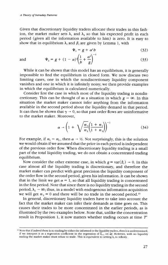
Given that discretionary liquidity traders allocate their trades in this fash- ion, the market maker sets X, and X2 so that his expected profit in each period (given all the information available to him) is zero. It is easy to show that in equilibrium Xt and at are given by Lemma 1, with
'1 = g + a2h (32)
and "2 = g + (1-a)2(! +- (33)
While it can be shown that this model has an equilibrium, it is generally impossible to find the equilibrium in closed form. We now discuss two limiting cases, one in which the nondiscretionary liquidity component vanishes and one in which it is infinitely noisy; we then provide examples in which the equilibrium is calculated numerically.
Consider first the case in which most of the liquidity trading is nondis- cretionary. This can be thought of as a situation in which g - co. In this situation the market maker cannot infer anything from the information available in the second period about the liquidity demand in that period. It can then be shown that y - 0, so that past order flows are uninformative to the market maker. Moreover,
a (+nl)) 1 1
(34)
For example, if n1 = n2, then a - /2. Not surprisingly, this is the solution we would obtain if we assumed that the price in each period is independent of the previous order flow. When discretionary liquidity trading is a small part of the total liquidity trading, we do not obtain a concentrated-trading equilibrium.
Now consider the other extreme case, in which g = var(C-) - 0. In this case almost all the liquidity trading is discretionary, and therefore the market maker can predict with great precision the liquidity component of the order flow in the second period, given his information. It can be shown that in the limit we get a = 1, so that all liquidity trading is concentrated in the first period. Note that since there is no liquidity trading in the second period, X2 - 00; thus, in a model with endogenous information acquisition we will get n2 = 0 and there will be no trade in the second period.'5
In general, discretionary liquidity traders have to take into account the fact that the market maker can infer their demands as time goes on. This causes their trades to be more concentrated in the earlier periods, as is illustrated by the two examples below. Note that, unlike the concentration result in Proposition 1, it now matters whether trading occurs at time T'
15 Note that if indeed there is no trading by either the informed or the liquidity traders, then A is undetermined, if we interpret it as a regression coefficient in the regression of 6, on CP. However, with no liquidity trading the market maker must refuse to trade. This is equivalent to setting A, to infinity.
27

The Review of Financial Studies / Spring, 1988
Table 6 Volume and price behavior when discretionary liquidity traders allocate trading across several periods
t n, X, VI V,' V, VIM Q, R,
1 3 0.43 4.73 1.73 1.00 2.00 0.25 2 4 0.30 7.84 2.67 2.19 2.99 0.20 1.05 3 3 0.38 6.51 2.12 1.95 2.45 0.25 0.95 4 3 0.40 6.31 2.06 1.87 2.38 0.25 1.00
A four-period example in which the number of informed traders, n,, is determined endogenously, assuming that the cost of information is 0.13 and that liquidity traders can allocate their trade in different periods between 2:00 P.M. and 4:00 P.M. For t = 1, 2, 3, 4, the table gives X,, the market-depth parameter; V,, a measure of total trading volume; V,1, a measure of the informed-trading volume; V7L, a measure of liquidity- trading volume; V,/, a measure of the trading volume of the market maker; Q,, a measure of the amount of private information revealed in the price; and R,, the variance of the price change from period t - 1 to period t.
or later; the different trading periods are not equivalent from the point of view of the discretionary liquidity traders. This will have implications when information acquisition is endogenous. Consider the following two exam- ples.
In the first example we make all the parametric assumptions made in our previous examples, except that now we allow the discretionary liquidity traders A and B to allocate their trades across periods 2, 3, and 4. If infor- mation acquisition is endogenous and if the cost of perfect information is c = 0.13, then we obtain the equilibrium parameters given in Table 6. In this example, each discretionary liquidity trader j trades about 0.4 Y' in period 2, 0.31 Yi in period 3, and 0.29Yi in period 4. Note that the measure of liquidity-trading volume is highest in period 2 and then falls off in periods 3 and 4. Three informed traders are present in each of the periods except period 2, when it is profitable for a fourth to enter. The behavior of prices is therefore similar to that when traders could only time their trades.
In the second example, illustrated in Table 7, we assume that there is less nondiscretionary liquidity trading. Specifically, we set the variance of nondiscretionary liquidity trading to be 0.1. With the cost of information at c = 0.04 and with endogenous information acquisition, we obtain pro- nounced patterns. For example, there are 11 informed traders in period 2 and three informed traders in each of the other periods. Liquidity trading is much heavier in period 2 as well, and the patterns of the volume and price behavior are very pronounced. In this example, each discretion- ary liquidity traderjtrades 0.74 Y'in period 2, 0.14Yjin period 3, and 0.12Ye in period 4.
5. Extensions
In this section we discuss a number of additional extensions of our basic model. We show that the main conclusions of the model do not change
28

A Tbeory of Intraday Patterns
Table 7 An example of pronounced patterns of volume and price behavior when discretionary liquidity traders allocate trading across several periods
t n, X, V, VI V, VIM Q R,
1 3 1.37 1.50 0.55 0.32 0.63 0.25 2 11 0.16 13.95 5.59 2.54 5.83 0.08 1.17 3 3 1.35 2.40 0.77 0.74 0.89 0.25 0.83 4 3 1.35 2.23 0.72 0.68 0.83 0.25 1.00
The same example as in Table 6, except that the variance of nondiscretionary liquidity trading is lower (0.1). The cost of information is assumed to be c = 0.04.
in more general settings. This indicates that our results are robust to a variety of models.
5.1 Different timing constraints for liquidity traders For simplicity, we have assumed so far that the demands of all the discre- tionary liquidity traders are determined at the same time and must be satisfied within the same time span. In reality, of course, different traders may realize their liquidity demands at different times, and the time that can elapse before these demands must be satisfied may also be different for different traders. Our results can be extended to this more general case, and their basic nature remains unchanged.
For example, suppose that there are three discretionary liquidity traders, A, B, and C, whose demands have the variances 5, 1, and 7, respectively. Suppose that trader A realizes his liquidity demand at 9:00 A.M. and must satisfy it by 2:00 P.M. that day. Trader B realizes his demand at 11:00 A.M.
and must satisfy it by 4:00 P.M., and trader C realizes his demand at 2:30 P.M. and must satisfy it by 10:00 A.M. on the following day. If each of these traders trades only once to satisfy his liquidity demands, then it is an equilibrium that traders A and C trade at the same time between 9:00 A.M.
and 10:00 A.M. (e.g., 9:30 A.M.) and that trader B trades sometime between 11:00 A.M. and 4:00 P.M.
Now suppose that the variance of B's demand is 9 instead of 1. Then the equilibrium described above is possible only if trader B trades before 2:30 P.M.; otherwise, trader C would prefer to trade at the same time that B trades rather than at the same time that A trades, and the equilibrium would break down. Two other equilibrium patterns exist in this situation. In one, traders B and C trade at the same time between 2:30 P.M. and 4:00 P.M. (e.g.,<3:00 P.M.), and trader A trades sometime between 9:00 A.M. and 2:00 P.M. In another equilibrium, traders A and B trade at the same time between 11:00 A.M. and 2:00 P.M. (e.g., 11:30 A.M.), and trader C trades sometime between 4:00 P.M. and 10:00 A.M. of the next morning. All these equilibria involve trading patterns in which two of the traders trade at the same time. If informed traders can enter the market, then their trading would also be concentrated in the periods with heavier liquidity trading.
29
The Review of Financial Studies / Spring, 1988
Thus, we obtain trading patterns similar to those discussed in the simple model.
5.2 Risk-averse liquidity traders We now ask whether our results change if, instead of assuming that all traders are risk-neutral, it is assumed that some traders are risk-averse. We focus on the discretionary liquidity traders, since their actions are the prime determinants of the equilibrium trading patterns we have identified. In the discussion below we continue to assume that informed traders and the market maker are risk-neutral. (A model in which these traders are also risk-averse is much more complicated and is therefore beyond the scope of this article.)
A risk-averse liquidity trader, say trader j, is concerned with more than the conditional expectation of Y'(P, - F) given his own demand Yi. Since he submits market orders, the price at which he trades is uncertain. In those periods in which a large amount of liquidity trading takes place, the variance of the order flow is higher. One may think that since this will make the price more variable, it will discourage risk-averse liquidity traders from trading together. In fact, the reverse occurs; that is, risk-averse li- quidity traders have an even greater incentive to trade together than do risk-neutral traders.
The following heuristic discussion uses the basic model of Sections 1 to 3. Given our assumptions, the conditional distribution of Pt - F is normal, given Yj and the public information available at time t. Thus, liquidity trader j is concerned only with the first two moments of this conditional distribution. Consider first the unconditional variance of Pt- F. Since Pt is the expectation of F, given the order flow at time t (and public information), the variance of Pt - Fis the variance of the prediction error. Suppose that all liquidity traders trade in period t*. Recall from Section 1 that because of the more intense trading by informed traders at t*, the prediction variance (which is related to Qt) is independent of It, the variance of liquidity trading. Thus, as long as the number of informed traders is constant over time, the concentration of liquidity trading in period t* does not increase the variance of Pt. - F relative to other pe- riods. We have also seen that the prediction variance is decreasing in ne, the number of informed traders. This implies that with endogenous infor- mation acquisition, since more informed traders trade in period t*, the prediction variance is even lower.
Now, liquidity trader j also knows his own demand Yi so we must con- sider the conditional variance of Pt - F, given Yi. If ft(n,) is the uncon- ditional variance discussed above, then the conditional variance is equal to f(nt) - X2 var( Y') if trader ] trades in period t and is equal to f(nt) if he trades in a different period. It is clear now that the fact that trader j knows Y' does not change the direction of the results outlined in the preceding paragraph; if all discretionary liquidity traders trade in period t* E [T', T"], then f*(n*) - X2* var(Y') < f(nt) for all tE [T', T"] and t '
30

A Theory of Intraday Patterns
t* and for all j. Thus, the equilibrium in which discretionary liquidity traders concentrate their trading in one period is still viable even if these traders are risk-averse.
5.3 Correlated demands of liquidity traders We have assumed that the demands of discretionary liquidity traders are independent of each other. This assumption seems to be reasonable if liquidity demands are driven by completely idiosyncratic life-cycle motives that are specific to individual traders. If liquidity demands are correlated across traders because of some common factors affecting these demands, and if these factors are observed by the market maker before he forms prices, then our analysis is still valid, with the interpretation that liquidity trading corresponds to the unpredictable part of these demands.
It is possible to extend our analysis to the case where common factors in liquidity demands are not observable (or, in general, to the case of correlated liquidity demands). Two considerations arise in this case. First, if liquidity traders trade in different periods, then past order flows may provide information to the market maker concerning the liquidity com- ponent in the current order flow. Second, if more than one liquidity trader trades in a given period, then the cost of trading in this period, which is proportional to the correlation of his demands with the total order flow, involves an additional term that reflects the correlation of the trader's demand with the other liquidity demands.
If liquidity demands are negatively correlated, then it can be shown that concentrated-trading equilibria always exist, so our results are still valid. The same is true if the variance of nondiscretionary liquidity demands is small enough, that is, if there is very little nondiscretionary liquidity trad- ing. The results may be different if liquidity demands are positively cor- related. In this case it is possible that an equilibrium in which trading is completely concentrated does not exist, or that equilibria in which different traders trade in different periods also exist, in addition to the concentrated- trading equilibria (and they are robust to slight perturbations in the param- eters). Examples are not difficult to construct.
6. Empirical Implications
The result that trading is concentrated in particular periods during the day and that the variability of price changes is higher in periods of concentrated trading is clearly consistent with empirical observations of financial mar- kets, as discussed in the Introduction and in the following section. Our models also provide a number of more specific predictions, examples of which we will spell out below. For simplicity, we will mostly use the model of Sections 1 to 3, where discretionary liquidity traders trade only once within the period in which they have to satisfy their liquidity demands.
In the context of our model, it seems reasonable to treat prices Pt and order flows ,t as observables. Specifically, if we define the periods to be,
31
The Review of Financial Studies / Spring, 1988
say, 30 minutes long, then the relevant price would be the last transaction price of the interval, and the order flow would be the net change in the position of the market maker during the interval. (It should be noted, however, that in practice the order-flow data may not be easily available from market makers.)
Suppose for simplicity that trading periods are divided into two types, those with high trading volume and those with low trading volume. We will use H and L to denote the set of periods with high and low trading volumes, respectively. (We also use superscript parameters accordingly.) The basic pricing equation in our model is
Pt=: aT + XH4Z,t (35) t=I
for periods with high volume (t E H) and
Pbt= 6T + XLt (36) T=l
for periods with low volume (tE L). Three hypotheses follow directly from our results in Sections 1 to 3.
Hypothesis 1. XH < XL.
That is, our model predicts that the market-depth coefficient (defined by 1/XA) is higher when the volume is lower. This hypothesis can easily be tested by using standard statistical procedures, as long as we can estimate XH and XL from price and order-flow observations. To see how this can be done, define
Mt=Pt+1-Pt-1 = bt+1 + bt + -t+1 t+ -At_1ut_i (37)
An estimate of XH can be obtained by regressing the observations of Mt for tE Hon the order-flow observations vt. This follows because all the terms in the above expression, except k, are independent of Uvt and because, by construction, Xt is set by the market maker as the regression coefficient in the prediction of bt+ 1, given vt . Similarly, a regression of the observations of mt for t E L on jt& would give an estimate of XL.16
Hypothesis 2. If t E H and t' E L, then Qt < Qt'; that is, var(6t+ Il Pt) <
var(Ot+1 I Pt)
This simply says that prices are more informative in periods in which the trading volume is heavier. Although it is less transparent to see, Hypothesis
16 Note that in the model of Section 4, where liquidity traders can allocate their trades, previous order flows miiust be included in the regression as well, since they (indirectly) provide relevant information in predicting 3t+2
32

A Theory of Intraday Patterns
2 can also be tested empirically using price and order-flow observations. This is shown in the Appendix.
Hypothesis 3. The variance of the price change from t E L to t + 1 E H is larger than the variance of the price change from tE L to t + 1 E L, and this exceeds the variance of the price change from t E H to t + 1 E L.
It is straightforward to test this hypothesis, given price and volume observations.
Cross-sectional implications can also be derived from our analysis. For example, it is reasonable to assume that a typical discretionary liquidity trader is a large institutional trader. Our models predict that trading pat- terns will be more pronounced for stocks that are widely held by these institutional traders.
7. Concluding Remarks
This article has presented a theory of trading patterns in financial markets. Some of the conclusions of our theory are these:
* In equilibrium, discretionary liquidity trading is typically concen- trated.
* If discretionary liquidity traders can allocate their trades across dif- ferent periods, then in equilibrium their trading is relatively more con- centrated in periods closer to the realization of their demands.
* Informed traders trade more actively in periods when liquidity trading is concentrated.
* If information acquisition is endogenous, then in equilibrium more traders become privately informed in periods of concentrated liquidity trading, and prices are more informative in those periods.
We have obtained our results in models in which the information process and the amount of nondiscretionary liquidity trading are completely sta- tionary over time. All the patterns we have identified in volume and price variability emerge as consequences of the interacting strategic decisions of informed and liquidity traders. The main innovation in our theory is the explicit inclusion of discretionary liquidity traders, who can time their trading. As discussed in the Introduction, observations similar to the last two points above have been made as comparative statics results in Kyle (1984), where the variance of liquidity trading is parametrically varied in a single period model. We have shown that these results continue to hold in equilibrium when the timing of liquidity trading is endogenized. As we have seen, it is a delicate matter whether the strategic interaction between liquidity traders and informed traders actually leads to pronounced patterns of trading over time. Among other things, what is important in this regard is the degree of competition among informed traders. When informed traders observe highly correlated signals, competition between them is
33

The Review of Financial Studies/ Spring, 1988
intense, and this improves the terms of trade for liquidity traders, promoting concentration of trading. If private signals are weakly correlated, however, then competition among informed traders is less intense, and an increase in the number of informed traders can actually worsen the terms of trade. This may lead to the nonexistence of an equilibrium. However, despite the complexity of the strategic interaction among traders, our analysis shows that whenever an equilibrium exists, it is characterized by the con- centration of liquidity and informed trading and by the resulting patterns in volume and price behavior.
The actual timing and shape of trading patterns in financial markets are determined by a number of factors and parameters that are exogenous to the model, such as the rate of arrival of public information, the amount of nondiscretionary liquidity trading, and the length of the interval within which each discretionary liquidity trader trades. As we noted, empirical observations suggest that the daily patterns in trading volume and returns are quite profound. In particular, there is heavier trading at the beginning and end of the trading day than there is in the middle of the day, and the returns and price changes are more variable.
There are a few hypotheses that, combined with our results, may explain the concentration of trading at the open and the close. The open and close are distinguished by the fact that they fall just after and just before the exchange is closed: that is, after and before a period of time in which it is difficult or impossible to trade. This may cause an increase in (nondis- cretionary) liquidity trading at the open and close. As a result, discretionary liquidity trading (as well as informed trading) will also be concentrated in these periods, as implied by our results. In this case the forces we have identified for concentration would be intensified.
The concentration of trading at the end of the trading day may also be due to the settlement rules that are followed by many exchanges. Under these rules all trades undertaken on a particular day are actually settled by the close several days later. While delivery depends on the day in which the transaction takes place, the exact time within a day in which the trade occurs has no effect on delivery. This suggests that the interval within which many discretionary liquidity traders must trade terminates at the close of a trading day, (i.e., that for many liquidity traders T" is the close of a trading day). Since T', the time at which liquidity demands are realized, may vary across traders, there will be a tendency for trading to be concen- trated at the close, when there is the most overlap among the intervals available to different liquidity traders. (See Section 5.1 for an intuitive discussion of this in the context of a related example.)
Note that the model of Section 4, in which discretionary liquidity traders can allocate their trades over different periods, predicts that trading will be concentrated in "earlier" trading periods (i.e., in periods closer to the time in which the liquidity demand is realized). For example, if many discretionary liquidity traders realize their liquidity demands after the market closes, then our model predicts that they will satisfy them as soon
34

A Theory of Intraday Patterns
as the market opens the next day. If, on the other hand, liquidity demands are realized late in the trading day, then we will observe heavy trading by discretionary liquidity traders and informed traders near the close of the market.
Our analysis may also shed some light on the finding discussed in French and Roll (1986) that the variance of returns over nontrading periods is much lower than the variance of returns over trading periods. If the li- quidity-trading volume is higher at the end of the trading day, then more informed traders will trade at this time. As a result, the prices quoted at the end of the trading day will reflect more of the information that will be released publicly during the following nontrading hours (see Hypothesis 2 in Section 6). While this effect may explain some of these findings, it is probably not sufficiently strong to account for the striking differences in variances reported in French and Roll (1986).
It is interesting to ask whether our results can account for the actual magnitudes of the observed patterns. A satisfactory answer to this question requires a serious empirical investigation, something we will not attempt here. However, casual calculations suggest that the predictions from the model may accord well with the observed magnitudes. For example, con- sider again the Exxon data presented in Table 1. Suppose that there are four informed traders in period 1 (10 A.M. to 12 noon), one informed trader in period 2 (12 noon to 2 P.M.), and three informed traders in period 3 (2 P.M. to 4 P.M.). These values are roughly consistent with the pattern of trading volume. Suppose also that 0 = 0; that is, informed traders in period thave perfect information about bt+, Finally, let U2 = 0.115661, the average of the variance of the price changes in the three periods. Then we can calculate the variance of price change in each period as predicted by our model using Equation (16), modified to include ,. (In doing this calcu- lation we ignore the overnight period and assume that the third period of one day immediately precedes the first period of the next.)
R (1 + 10.34849 + n, 1 + n 3
'/2
_ _ _ 1 R=( + 9 ) 0.28454
(i+n2 1
_ _ _ _ 1 N R=' ( + = 0.38023 3
1 + n 1 + fl2/
These values are quite close to the observed values (0.34959, 0.28371, 0.37984).17 The foregoing should in no way be construed as a test of the
17 We have in fact searched over a number of possible candidates for (n1, n, n3) and have obtained the best fit with (4, 1, 3).
35
The Review of Financial Studies/ Spring, 1988
model. We simply conclude that the effects the model predicts can be of the same magnitude as those seen in the data.
In closing, we note that many intraday phenomena remain unexplained. For example, a number of studies have shown that mean returns also vary through the day. [See, for example, Jain and Joh (1986); Harris (1986); Marsh and Rock (1986); and Wood, Mclnish, and Ord (1985).] In our model, prices are a martingale, so patterns in means do not arise. This is due in part to the assumption of risk neutrality. [Williams (1987) analyzes a model that is related to ours in which risk aversion plays an important role and mean effects do arise.] Developing additional models that produce testable predictions for transaction data is an important task for future research.
Appendix
Proof of Lemma 1 Consider the informed traders' decisions. The ith informed trader chooses xi, the amount to trade in period t, to maximize the expected profits, which are given by
E(xti(F - Pt(At, Qt)) I At Qt-1 bt+1 + et) (Al)
Given the form of the price function in Equation (3), this can be written as
E(xti(6l-Xt) &t+l + et) (A2)
Suppose that informed trader i conjectures that the market order of the other n - 1 informed traders is equal to t(6t+l1 + et). Then the total order flow is (3t = xti + (nt - 1)f(b, + Et) + Xj=l ji + t, and the ith informed trader chooses xti to maximize
ELxtt+1 x-xti(xt + (n, - 1)ft,(t+l + e,) + ) j +
which is equal to
xtvar(5t+l) (6 + et) - x;Xt(xi + (n, - l)#t(6t+1 + et)) (A4) var(bt+l) + 4t
It is easily seen that the expected profits of the ith informed trader in period t are maximized if xi is set equal to
( vrt+ 1) _ n 1- i)j3, + et) (A5) 2X,(var(bt+,) + 4t) 2
The Nash equilibrium is found by setting the above equal to ft(b?1 +
et) and solving for t.118 We obtain
36
A Theory of Intraday Patterns
ot ~~var(bt+1) 6 (n, + I)Xt(var(&,+1) + )) (A6)
We now determine the value of X, for a given set of strategies by all traders. Recall that the total amount of discretionary liquidity demands in period t is -1 5/, where 5/ = Yi if the jth discretionary liquidity trader trades in period t and where 5j = 0 otherwise. The zero-profit condition for the market maker implies that
cov(bt+1, nt) _ nt var(Gt+1) xt var(c7') nf232(var3t+1) + 4t) + it
(A7)
Substituting Equation (A6) for Ot, we obtain a cubic equation for Xt. The unique positive root gives the equilibrium value for the assumed level of liquidity trading. This is the value given in Equation (5). U
Proof of Lemma 2 As shown in the proof of Lemma 1, when nt traders are informed, each places in period t a market order of 3t(Qt+l + et) shares, where
= (nt + 1)X(nt, *t')(1 + 4) (A8)
[We assume here that var(3t+1) = 1 and 4)t = 0.] Now consider a deviant trader who acquires information in addition to the other n traders. He will demand xt shares, where xt maximizes
E[xt(-t+l X(nt, 't)(xt + nt0t(bt+1 + et) + it)) I bt+l + et] (A9)
where u-t is the total liquidity demand in period t. This is maximized at
xt = (2X(f I7)l + + et) (AIO) t2X(nt, *t,) (1 + f ) 2 )(t , A0
or substituting for ft,
=
( nt, x
t,) (1 + 0)pi 2 (nt + l) X( nt, t) (1 + 0)) (&? + et)
2(nt + 1)X(nt, 'tI)(1 + 4))
2 + l t) (A1) 2 te I
The expected profits earned by the deviant trader, lr d(nt, 'It), will be
18 It is straightforward to prove that the equilibrium among informed traders is always unique.
37
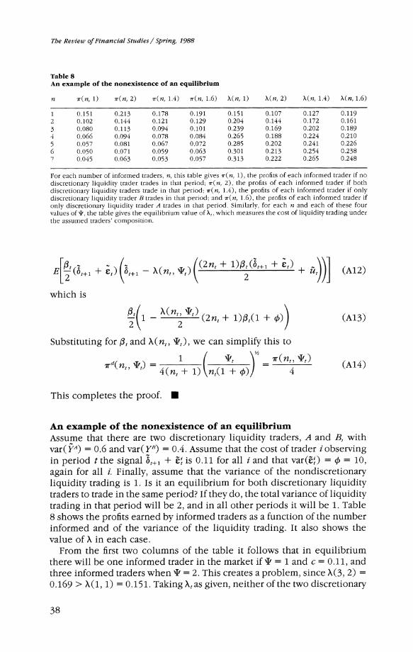
The Review of Financial Studies/ Spring, 1988
Table 8 An example of the nonexistence of an equilibrium
n 1r(n, 1) 7r(n, 2) 7r(n, 1.4) lr(n, 1.6) X(n, 1) X(n, 2) X(n, 1.4) X(n, 1.6)
1 0.151 0.213 0.178 0.191 0.151 0.107 0.127 0.119 2 0.102 0.144 0.121 0.129 0.204 0.144 0.172 0.161 3 0.080 0.113 0.094 0.101 0.239 0.169 0.202 0.189 4 0.066 0.094 0.078 0.084 0.265 0.188 0.224 0.210 5 0.057 0.081 0.067 0.072 0.285 0.202 0.241 0.226 6 0.050 0.071 0.059 0.063 0.301 0.213 0.254 0.238 7 0.045 0.063 0.053 0.057 0.313 0.222 0.265 0.248
For each number of informed traders, n, this table gives lr(n, 1), the profits of each informed trader if no discretionary liquidity trader trades in that period; ir(n, 2), the profits of each informed trader if both discretionary liquidity traders trade in that period; 7r(n, 1.4), the profits of each informed trader if only discretionary liquidity trader B trades in that period; and xr(n, 1.6), the profits of each informed trader if only discretionary liquidity trader A trades in that period. Similarly, for each n and each of these four values of I, the table gives the equilibrium value of X,, which measures the cost of liquidity trading under the assumed traders' composition.
[ / ~ ~~~~~(2t+ 1)ftljt?l + et)
E #t(bt+l + et) 6tr+ - X(nt, i,)(( ' 2 + (A12)
which is
'( 1 - X(nt, 't) (2nt + 1)flt(l + {i)) (Al 3)
Substituting for ft and X(nt, *t), we can simplify this to
7 d( nt, 't) = 4(An 1+1) ( ( ) 4 (A14)
This completes the proof. U
An example of the nonexistence of an equilibrium Assume that there are two discretionary liquidity traders, A and B, with var( yA) = 0.6 and var( yB) = 0.4. Assume that the cost of trader i observing in period t the signal &t+ + Ei is 0.11 for all i and that var(i) = = 10, again for all i. Finally, assume that the variance of the nondiscretionary liquidity trading is 1. Is it an equilibrium for both discretionary liquidity traders to trade in the same period? If they do, the total variance of liquidity trading in that period will be 2, and in all other periods it will be 1. Table 8 shows the profits earned by informed traders as a function of the number informed and of the variance of the liquidity trading. It also shows the value of X in each case.
From the first two columns of the table it follows that in equilibrium there will be one informed trader in the market if J = 1 and c = 0.11, and three informed traders when I = 2. This creates a problem, since A(3, 2) = 0.169 > X(1, 1) = 0.15 1. Taking Xt as given, neither of the two discretionary
38
A Tbeory of Intraday Patterns
liquidity traders will be content to trade in the period they are assumed to trade in. If each assumes that he can move to another period without affecting other traders' strategies, then each will want to move to one of the periods with X = 0.151.
Having shown that it is not an equilibrium for both A and B to trade in the same period, we now show that it is also not an equilibrium for each discretionary liquidity trader to trade in a different period. From the third and fourth columns of the table it follows that if each discretionary liquidity trader trades in a different period, then there will be two informed traders in each period. However, in the period in which A trades, X = X(2, 1.6) = 0.161, while in the period in which B trades, X = X(2, 1.4) = 0.172. If B takes the strategies of all other traders and Xt as given, he will want to trade in the period in which A is trading.
A statistical test of hypothesis 2 Note first that Qt= var(Gt,j - E(Gt+j I't)) = var(Gt+j -Xtt). Thus, Hypoth- esis 2 is equivalent to the hypothesis that if t E H and t' E L, then
Var(6t+l -Xt t) < var(6t+1 - Xt'It') (A15) Since at = +- 1 -Pt -Xt+j??t+1 + XtZCt, Equation (A15) is equivalent to
var(Pt+l- Pt - Xt+jt+) < var(Pt,+1 - Pt'- Xt'+1t1) (A16)
Denote the estimates of XH and XL, obtained by the regression described after Hypothesis 1, by XH and XL. Suppose that these are estimated out of sample. Also assume for simplicity that both t + 1 and t' + 1 are periods with low trading volume.19 Then Hypothesis 2 can be tested by comparing var(Pt+ 1 - Pt- XLt+) with var (Pt,+ - Pt - XLC+t,+) .To see this, note that
var(Pt+I - Pt- XLOt+j) = var(Pt+l - Pt - XLJ,t+) + var(XL - XL) var(?t+1)
+ 2 cov((XL - XL)ot+?1, Pt+1 - Pt - XL&t+1) (A17)
The covariance term is zero (since XL is estimated out of sample), and the second term on the right-hand side is the same whether the trading volume is high or low at time t, as long as the trading volume is low in period t + 1. Thus, Equation (A16) can be tested by comparing var(Pt+1 -Pt - XL t+l) with var(Pt,+1 - Pt- X t'+)
References Clark, P. K., 1973, A Subordinated Stochastic Process Model with Finite Variance for Speculative Prices, Econometrica, 41, 135-155.
Foster, F. D., and S. Viswanathan, 1987, Interday Variations in Volumes, Spreads and Variances: I. Theory, Working Paper 87-101, Duke University, The Fuqua School of Business, October.
19 The case in which both are periods with high trading volume is completely analogous. Otherwise, the discussion can be modified in a straightforward manner.
39

The Review of Financial Studies/ Spring, 1988
French, K. R., and R. RoIl, 1986, Stock Return Variances; the Arrival of Information and the Reaction of Traders, Journal of Financial Economics, 17, 5-26.
Glosten, L. R., and P. R. Milgrom, 1985, Bid, Ask and Transaction Prices in a Specialist Market with Heterogeneously Informed Traders, Journal of Financial Economics, 14, 71-100.
Harris, L., 1986, A Transaction Data Survey of Weekly and Intraday Patterns in Stock Returns, Journal of Financial Economics, 16, 99-117.
Jain, P. J., and G. Joh, 1986, The Dependence Between Hourly Prices and Trading Volume, working paper, University of Pennsylvania, Wharton School.
Kyle, A. S., 1984, "Market Structure, Information, Futures Markets, and Price Formation," in International Agricultural Trade: Advanced Readings in Price Formation, Market Structure, and Price Instability, ed. by Gary G. Storey, Andrew Schmitz, and Alexander H. Sarris. Boulder and London: Westview Press, 45- 64.
Kyle, A. S., 1985, Continuous Auctions and Insider Trading, Econometrica, 53, 1315-1335.
Marsh, T. A., and K. Rock, 1986, The Transaction Process and Rational Stock Price Dynamics, working paper, Berkeley, University of California.
Williams, J., 1987, Financial Anomalies Under Rational Expectations: A Theory of the Annual Size and Related Effects, working paper, New York University, Graduate School of Business Administration.
Wood, R. A., T. H. Mclnish, and J. K. Ord, 1985, An Investigation of Transaction Data for NYSE Stocks, Journal of Finance, 40, 723-741.
40