IEEE CONFERENCE ON DECISION AND CONTROL (CDC), PREPRINT VERSION. ACCEPTED JULY, 2021. 1

A Theoretical Overview of Neural Contraction Metrics forLearning-based Control with Guaranteed Stability

Hiroyasu Tsukamoto∗, Soon-Jo Chung∗, Jean-Jacques Slotine†, and Chuchu Fan‡

Abstract—This paper presents a theoretical overview of aNeural Contraction Metric (NCM): a neural network model ofan optimal contraction metric and corresponding differentialLyapunov function, the existence of which is a necessary andsufficient condition for incremental exponential stability of non-autonomous nonlinear system trajectories. Its innovation liesin providing formal robustness guarantees for learning-basedcontrol frameworks, utilizing contraction theory as an analyticaltool to study the nonlinear stability of learned systems via convexoptimization. In particular, we rigorously show in this paperthat, by regarding modeling errors of the learning schemes asexternal disturbances, the NCM control is capable of obtaining anexplicit bound on the distance between a time-varying target tra-jectory and perturbed solution trajectories, which exponentiallydecreases with time even under the presence of deterministic andstochastic perturbation. These useful features permit simultane-ous synthesis of a contraction metric and associated control lawby a neural network, thereby enabling real-time computable andprobably robust learning-based control for general control-affinenonlinear systems.

I. INTRODUCTION

Since the development of reinforcement learning and neuralnetworks [1], [2], leveraging Artificial Intelligence (AI) andMachine Learning (ML) methods in the field of systems andcontrol theory has been an active field of research. Althoughsuccessful, conventional black-box AI and ML approachesoften lack formal robustness and stability guarantees, whichare essential in implementing safety-critical control schemesfor, e.g., robotic and aerospace systems.

Related Work: Contraction theory is one of the mostpowerful mathematical tools for providing such guaranteesfor learning-based control frameworks [3], [4]. GeneralizingLyapunov theory, it studies differential dynamics of a non-linear system using a Riemannian contraction metric andits uniformly positive definite matrix, thereby designing adifferential Lyapunov function to characterize a necessary andsufficient condition for exponential convergence of any coupleof the system trajectories. Due to the differential nature ofcontraction theory which allows utilizing LTV system-typeapproaches [4]–[8], its nonlinear stability analysis reduces tothe problem of finding a contraction metric that satisfies aLinear Matrix Inequality (LMI) [9].

Obtaining contraction metrics analytically is challengingfor general nonlinear systems, and thus several techniqueshave been proposed to find them numerically using the LMIproperty. In particular, it is proposed in [10] that sufficient con-ditions for incremental exponential stabilizability of nonlinear

∗ Graduate Aerospace Laboratories, Caltech, Pasadena, CA,{htsukamoto, sjchung}@caltech.edu.

† Nonlinear Systems Laboratory, MIT, Cambridge, MA, jjs@mit.edu.‡ Reliable Autonomous System Laboratory, MIT, Cambridge, MA,

chuchu@mit.edu.

systems can be expressed as convex constraints, enablingsystematic synthesis of a differential feedback control. Suchan idea is further extended to develop the method of ConVexoptimization-based Steady-state Tracking Error Minimization(CV-STEM) [4]–[7], which computes a contraction metricand its associated feedback control and state estimation lawsvia convex optimization for optimal deterministic/stochasticdisturbance attenuation.

A critical limitation of these optimization-based schemesis their computational complexity. In essence, a Neural Con-traction Metric (NCM) and its extensions [4], [6]–[8], [11],[12] are developed to model the CV-STEM contraction metricusing a Deep Neural Network (DNN), achieving real-timeimplementable control, estimation, and motion planning ofnonlinear systems with guaranteed robustness and stability.We again remark that such formal guarantees are difficultto quantify for black-box AI and ML techniques withoutconsidering a contracting stability property.

Contribution: This paper presents rigorous proofs on theaforementioned theoretical guarantees of the NCM meth-ods [4], [6]–[8], [11], [12], which provide an explicit ex-ponential bound on the distance between a target trajectoryand solution trajectories with the NCM learning-based control,even under the presence of learning errors and determinis-tic/stochastic perturbation. We also derive one explicit wayto optimally sample NCM training data by formulating theCV-STEM, to design contracting differential feedback con-trol that minimizes the steady-state of the computed boundfor optimal disturbance attenuation. Furthermore, we providean algorithmic overview on DNN training for simultaneoussynthesis of the contraction metric and control, to see howthe NCM robustness and stability guarantees corroborate thesuccess of learning-based control.

Notation: For x ∈ Rn and A ∈ Rn×m, we let ‖x‖, δx, ‖A‖,and ‖A‖F denote the Euclidean norm, infinitesimal displace-ment at a fixed time, induced 2-norm, and Frobenius norm,respectively. For A ∈ Rn×n, we use A � 0, A � 0, A ≺ 0,and A � 0 for the positive definite, positive semi-definite,negative definite, negative semi-definite matrices, respectively,and sym(A) = (A+A>)/2. Also, E denotes the expected valueoperator.

II. NEURAL CONTRACTION METRICS FORLEARNING-BASED CONTROL [4], [6]–[8], [12]

In this paper, we consider the following smooth non-autonomous (i.e. time-varying) nonlinear system, perturbed bydeterministic disturbances d(x, t) with supx,t ‖d(x, t)‖= d andGaussian white noise W (t) with ‖G(x, t)‖F ≤ g:

dx =h(x,u, t)dt +d(x, t)dt +G(x, t)dW (t) (1)

© 2021 IEEE. Personal use of this material is permitted. Permission from IEEE must be obtained for all other uses, in any current or future media,including reprinting/republishing this material for advertising or promotional purposes, creating new collective works, for resale or redistribution to servers

or lists, or reuse of any copyrighted component of this work in other works. Digital Object Identifier (DOI): TO BE ASSIGNED.

arX

iv:2

110.

0069

3v1

[cs

.LG

] 2

Oct

202

1

2 IEEE CONFERENCE ON DECISION AND CONTROL (CDC), PREPRINT VERSION. ACCEPTED JULY, 2021.

where t ∈ R+, x : R+ 7→ Rn is the system state, u ∈ Rm isthe system control input, h : Rn×Rm×R+→ Rn is a knownsmooth function, d : Rn×R+ 7→Rn and G : Rn×R+→Rn×w

are unknown bounded functions for external disturbances, W :R+ 7→Rw is a w-dimensional Wiener process, and we considerthe case where d, g ∈ [0,∞) are given. Let us first introducethe following definition of contraction [3].

Definition 1. The system (1) is said to be contracting ifthere exist a uniformly positive definite matrix M(x, t) =Θ(x, t)T Θ(x, t) � 0, ∀x, t and a feedback control law u =u∗(x,xd ,ud , t) s.t. the following condition holds ∀x, t:

M+2sym(

M∂h(x,u∗(x,xd ,ud , t), t)

∂x

)+Ξ(x, t)� 0 (2)

where ∃Ξ(x, t) � 0, ∀x, t, M = M(x, t), and xd is the targettrajectory of (1) given as follows:

xd = h(xd ,ud , t) s.t. ud = u∗(xd ,xd ,ud , t). (3)

We call M and u∗ satisfying (2) a contraction metric andcontracting control law, respectively.

It is shown that (2) is a necessary and sufficient conditionfor incremental exponential stability of the system trajectorieswith respect to each other [3], [4].

A. Problem Formulation

Finding an optimal contraction metric M for general non-linear systems is challenging and could involve solving opti-mization problems at each time instant [5], [13] (see Sec. III),which is not suitable for systems with limited computationalcapacity. A Neural Contraction Metric (NCM) and its exten-sions [4], [6]–[8], [12] have been proposed to approximate acontracting control law u∗, i.e., a computationally-expensivecontrol law parameterized by the contraction metric given by(2), utilizing a Deep Neural Network (DNN).

Definition 2. A Neural Contraction Metric (NCM) is a DNNmodel of a contraction metric given by Definition 1.

We consider the problem of modeling the contracting con-trol law u∗ by a learning-based control law uL(x,xd ,ud , t)parameterized by the NCM of Definition 2 (see [5], [10] andSec. III for how to obtain u∗). Let x be the trajectory of (1)controlled by u = uL, and xd be the target trajectory of (3).Since we have h(x,uL, t) = h(x,u∗, t)+(h(x,uL, t)−h(x,u∗, t)),a virtual system of q, which has q = x and q = xd as itsparticular solutions, is given as follows:

dq = h(q,u∗(q,xd ,ud , t), t)dt +dq(q, t)dt +Gq(q, t)dW (4)

where dq and Gq are parameterized linearly to verifydq(q = xd , t) = 0, dq(q = x, t) = h(x,uL(x,xd ,ud , t), t) −h(x,u∗(x,xd ,ud , t), t)+ d(x, t), Gq(q = xd , t) = 0, and Gq(q =x, t) = G(x, t).

Assumption 1. In this section, we assume the following.• For all (x,xd ,ud , t) ∈ S, uL is learned to satisfy

‖uL(x,xd ,ud , t)−u∗(x,xd ,ud , t)‖ ≤ ε`0 + ε`1

∫ x

xd

‖δq‖ (5)

where S = Sx×Sx×Su×St , Sx ⊂Rn, Su ⊂ Rm, and St ⊂ R+

are some given compact sets, and∫ x

xd‖δq‖ is a path integral

from xd to x parameterized by q of (4).• h of (1) is Lipschitz with respect to u, i.e., ∃Lu ∈ [0,∞) s.t.

‖h(x,u, t)−h(x,u′, t)‖ ≤ Lu‖u−u′‖, ∀u,u′ ∈ Rm (6)

for all x ∈ Sx and t ∈ St .• Let Sxt = Sx× St . When G 6= 0 in (1), ∂M/∂xi of M in (2)is Lipschitz with respect to x, i.e., ∃Lm ∈ [0,∞) s.t.∥∥∥∥∂M

∂xi(x, t)− ∂M

∂xi(x′, t)

∥∥∥∥≤ Lm‖x− x′‖, ∀(x, t),(x′, t) ∈ Sxt .

(7)

Remark 1. (5) can be empirically guaranteed, e.g., by DNNs,which have been shown to generalize well to the set of unseenevents that are from almost the same distribution as theirtraining set [14], [15], and consequently, obtaining a tighterand more general bound for the learning error has beenan active field of research [16]. The condition (5) has thusbecome a common assumption in analyzing the performanceof learning-based control [4], [8], [12], [15].

B. Nonlinear Robustness and Stability Analysis

The following theorem rigorously studies robustness andstability of the NCM-parameterized control law uL.

Theorem 1. Suppose that Assumption 1 holds. Suppose alsothat the contraction metric M(x, t) of (2) is bounded as

mI �M(x, t)� mI, ∀x, t (8)

for ∃m,m ∈ (0,∞), and u∗ of (2) is given with Ξ defined as

Ξ(x, t) = 2αM(x, t)+αsI (9)

where ∃α ∈ (0,∞) is the contraction rate and αs = Lmg2(αG+1/2) with an arbitrary constant αG ∈ (0,∞) (see (14)). If thelearning error ε`1 of (5) and another arbitrary constant αd ∈(0,∞) (see (15)) are selected to satisfy

∃α` ∈ (0,∞) s.t. α` = α− (αd/2+Luε`1√

m/m)> 0 (10)

then we have the following bound for all (x, t) ∈ Sx×St :

E[‖x(t)− xd(t)‖2]≤ C

2α`

mm+

E[Vs`(0)]e−2α`t

m(11)

where Vs`(t) =∫ x

xdδq(t)>M(q(t), t)δq(t), C = g2(2αG

−1 +

1)+ (Luε`0 + d)2α−1d , d, g, and q are given in (1) and (4),

x is the trajectory of (1) controlled by u = uL, and xd is thetarget trajectory given by (3).

Proof. Since ∂M/∂xi is Lipschitz as in (7), we have‖∂ 2M/(∂xi∂x j)‖ ≤ Lm and ‖∂M/∂xi‖ ≤

√2Lmm using (8) as

derived in [7]. Also, dq of (4) is bounded as

‖dq(x, t)‖ ≤ Lu(ε`0 + ε`1

∫ x

xd

‖δq‖)+ d (12)

by the Lipschitz condition (6) and learning error bound (5).Let L be the infinitesimal differential generator in [17, p.15]. Since we have

∫ xxd‖δq‖ ≤ V`/

√m and V 2

` ≤ Vs` [4] for

H. TSUKAMOTO et al.: A THEORETICAL OVERVIEW OF NEURAL CONTRACTION METRICS FOR LEARNING-BASED CONTROL 3

V` =∫ x

xd‖Θδq‖ and M = Θ>Θ, computing LVs` using these

bounds as in [5] yields

LVs` ≤∫ x

xd

δq>(M+2sym(Mhx))δq+2Luε`1√

m/mVs`

+2√

mdεV`+ g2(m+∫ x

xd

Lm‖δq‖2/2+2√

2Lmm‖δq‖) (13)

where hx = ∂h/∂x and dε = Luε`0 + d. Using the relation2ab≤ c−1a2+cb2 which holds for any a,b∈R and c∈ (0,∞),we have that

2√

mdε‖Θδq‖ ≤αd‖Θδq‖2 +md2ε α−1d (14)

2√

2Lmm‖δq‖ ≤LmαG‖δq‖2 +2mα−1G (15)

for any αd ,αG ∈ (0,∞). Substituting (14) and (15) into (13)along with the contraction condition (2) for u∗ yields

LVs` ≤∫ x

xd

δq>(−Ξ+(αd +2Luε`1√

χ)M+αsI)δq+mC

where χ = m/m, αs = Lmg2(αG +1/2), and C = g2(2αG−1 +

1)+ d2ε α−1d . Thus, by definition of Ξ in (9), we have LVs` ≤

−2α`Vs`+mC due to the condition (10). This results in thedesired relation (11) due to Theorem 1 of [5].

Theorem 1 states that, as long as we have a contractingcontroller u∗ which satisfies (2) of Definition 1, the NCMcontroller uL of (5) ensures that the mean-squared distancefrom any target trajectory xd controlled by ud = u∗(xd ,xd ,ud , t)to the one controlled by uL with deterministic and stochasticperturbation is exponentially bounded in time, even under thepresence of the learning error ε`0 and ε`1. Such an explicitexponential bound is difficult to obtain for systems without acontraction property.

In particular, when there is no stochastic disturbance in thesystem (1), i.e., G = 0, we have the following result.

Theorem 2. Suppose (5) and (6) of Assumption 1 hold foru∗ that satisfies (2) with Ξ = 2αM(x, t), where ∃α ∈ (0,∞)is the contraction rate. Now let xd be the target trajectory of(3), and x be the trajectory controlled by uL with G = 0. If Mis bounded as in (8), and if the learning error ε`1 of (5) issufficiently small to satisfy

∃α` ∈ (0,∞) s.t. α` = α−Luε`1√

m/m > 0 (16)

then we have the following bound:

‖x(t)− xd(t)‖ ≤‖V`(0)‖√

me−α`t +

Luε`0 + dα`

√mm(1− e−α`t)

(17)

where V`(t) =∫ x

xd‖Θ(q(t), t)δq(t)‖ and q is given by (4) with

the same dq and Gq = 0 (note that this virtual system indeedhas q = x and q = xd as its particular solutions).

Proof. Let V = δq>Mδq. Using (13) computed in the proofof Theorem 1, along with the bound on dq (12) and thecontraction condition (2) for Ξ = 2αM, we have that

V ≤−2αV +2√

m(Lu(ε`0 + ε`1V`/√

m)+ d)‖Θδq‖ (18)

where the relation∫ x

xd‖δq‖ ≤V`/

√m is used. Since we have

V = ‖Θδq‖(d‖Θδq‖/dt) and V = ‖Θδq‖2, (18) implies that

V` ≤ −(α − Luε`1√

m/m)V` +√

m(Luε`0 + d), which resultsin (17) by applying the comparison lemma [18, pp.102-103,pp.350-353] as long as the condition (16) holds.

III. A CONVEX OPTIMIZATION APPROACH FOR NCMROBUST CONTROL [4]–[8]

Although Theorems 1 and 2 are already useful for systemswith a known contraction metric and corresponding differ-ential Lyapunov function, finding them for general nonlinearsystems is not always straightforward. This section delineatesone approach, called ConVex optimization-based Steady-stateTracking Error Minimization (CV-STEM), to optimally designu∗ and M of Theorem 1 for control-affine nonlinear systems,thereby demonstrating how to construct the NCM of Defini-tion 2 in practice for probably stable learning-based robustcontrol.

Let us consider the following control-affine nonlinear sys-tem:

dx =( f (x, t)+B(x, t)u)dt +d(x, t)dt +G(x, t)dW (t) (19)

where t, x, u, d, G, and W are as defined in (1), and f :Rn×R+→ Rn and B : Rn×R+→ Rn×m are known smoothfunctions.

Remark 2. If h(x,u, t)− ( f (x, t)+B(x, t)u) is bounded in (1)and (19), we can still apply the technique to be discussed inthis section even for control non-affine systems (1), by treatingthis modeling error as external disturbance d in (19). Forsituations where such an assumption is not valid, we couldapply (learning-based) adaptive control [8], [15], [19], [20]to estimate the non-affine part of the dynamics.

A. Contraction Theory-based Robust Control (CV-STEM)

We design a contracting control law u = u∗ for (19) by thefollowing differential feedback control law [10] (see Remark 3for more options):

u∗(x,xd ,ud , t) = ud−∫ x

xd

R(q, t)−1B(q, t)>M(q, t)δq (20)

where R(x, t) � 0 is a given weight matrix, M(x, t) � 0 is acontraction metric to be defined in Theorem 3, q is a smoothpath that connects x to xd as in (4), and xd is a given targettrajectory of (3) with h(x,u, t) = f (x, t)+B(x, t)u. Note that(20) yields δu∗ =−R(x, t)−1B(x, t)>M(x, t)δx.

Remark 3. We could utilize other types of control laws in(20), e.g., δu = k(x,δx,u, t) (see Sec. IV) [10] or u = ud −K(x,xd ,ud , t)(x− xd) [5]–[8]. See [4] for their trade-offs.

The CV-STEM is for designing u∗ and M of Theorem 1explicitly by (20) to minimize the steady-state bound of (11).

Theorem 3. Suppose that the contraction metric M(x, t) =W (x, t)−1 � 0 of (20) is designed by the following convexoptimization (CV-STEM) [4]–[7], which minimizes the steady-state upper bound of (11):

J∗CV = minν>0,χ∈R,W�0

C2α`

χ s.t. (22), (23), and (24) (21)

4 IEEE CONFERENCE ON DECISION AND CONTROL (CDC), PREPRINT VERSION. ACCEPTED JULY, 2021.

with the convex constraints (22), (23), and (24) given as[H(ν ,W )+2αW W

W να−1s I

]� 0, ∀x, t (22)

−∂biW +2sym(

∂bi

∂xW)= 0, ∀i = 1, · · · ,m, ∀x, t (23)

I � W (x, t)� χI, ∀x, t (24)

where ∂pF = ∑nk=1(∂F/∂xk)pk for p(x, t) ∈ Rn and F(x, t) ∈

Rn×n, ν = m, χ = m/m, W = νW, f and B are given in (19),bi is the ith column of B, and

H(ν ,W ) =−∂W∂ t−∂ fW +2sym

(∂ f∂x

W)−νBR−1B>.

with the other variables defined in Theorem 1. If u∗ isdesigned as (20) for M of (21), the contraction condition (2)of Definition 1 and (8) of Theorem 1 hold with Ξ given by (9),h(x,u, t) = f (x, t)+B(x, t)u, and u = u∗.

Proof. Applying Schur’s complement lemma [9, pp. 7] to theconstraint (22), we have that

H(ν ,W )+2αW −αsW 2/ν � 0. (25)

It can be easily verified that, by multiplying the constraints(25), (23), and (24) by M =W−1 from both sides and by ν−1,they can be equivalently rewritten as [5]

∂M∂ t

+∂ f M+2sym(M(∂ f/∂x))−MBR−1B>M �−Ξ (26)

∂biM+2sym(M(∂bi/∂x)) = 0 (27)mI �M � mI (28)

respectively, for Ξ of (9), where (28) indicates that (24) isindeed equivalent to (8). Combining (26) and (27), we get

M+2sym(M(∂ ( f (x, t)+B(x, t)u∗)/∂x))�−Ξ

which implies the contraction condition (2) holds forh(x,u, t) = f (x, t)+B(x, t)u and u = u∗.

Furthermore, it can be seen that the problem (21) minimizesthe steady-state upper bound of (11) due to the relationlimt→∞E

[‖x(t)− xd(t)‖2

]= (C/(2α`))(m/m) = (C/(2α`))χ .

Note that (21) is convex as the objective is affine in χ , and(22), (23), and (24) are linear matrix inequalities in terms ofν , χ , and W [9, pp. 7].

B. NCM Construction using CV-STEM

Now that we can construct the contracting control law u∗

of Theorem 1 by using Theorem 3, we are ready to explicitlydesign the NCM of Definition 2. Since the NCM only requiresone DNN evaluation at each time instant without solving anyoptimization problems unlike the CV-STEM of Theorem 3,it enables real-time computation of optimal feedback controlusing (20) in most engineering and science applications. Weformally derive its robustness and stability guarantees in thefollowing theorems.

Theorem 4. Let uL be a learning-based controller, prameter-ized by the NCM of Definition 2, which approximates the con-tracting control law u∗ of (20). If Assumption 1 holds for such

Find contraction metric givenby 𝑀 that minimizes 𝐷

𝑥 𝑡 , 𝑡

𝑦 𝑡 , 𝑡 NCM estimationneural net

𝑢(𝑥, 𝑡)

*𝑥(𝑡)

Compute 𝑢(𝑥, 𝑡) & *𝑥(𝑡)using trained neural nets

time 𝑡

{𝑥!}!"#$

Neural Network

＊1 & 2 via convex optimization (CV-STEM) ＊different nets for estimation & control

𝛿𝑥(𝑡)

𝛿𝑥(∞)𝐷

OFFLINEPHASE

ONLINEPHASE

{𝑡!}!"#$

{𝑀!}!"#$ NCM controlneural net

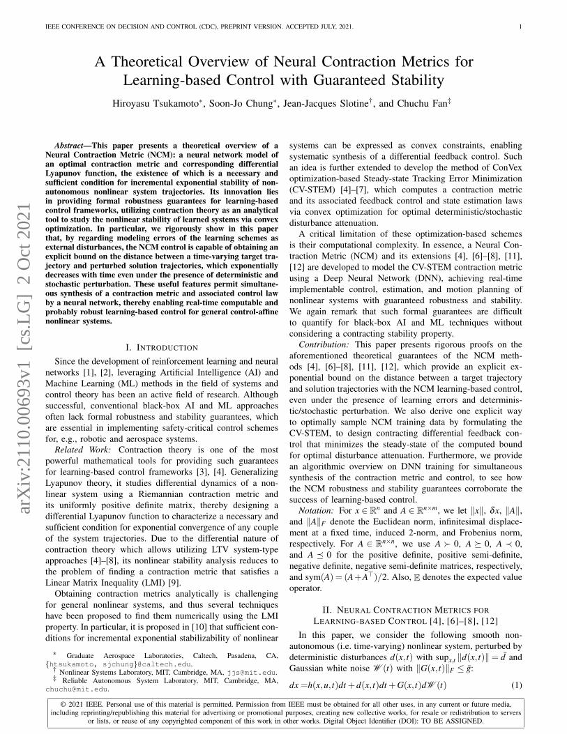
Fig. 1. Illustration of NCM (x: system state; M: positive definite matrix thatdefines optimal contraction metric; xi and Mi: sampled x and M; x: estimatedsystem state; y: measurement; and u: system control input). Note that thetarget trajectory (xd ,ud) is omitted in the figure fore simplicity. (see [4], [6]for state estimation).

uL, u∗, and M of Theorem 3 with h(x,u, t)= f (x, t)+B(x, t)u of(19), then Theorem 1 holds, i.e., the system trajectory of (19)controlled by uL exponentially converges to a ball around thetarget trajectory xd of (3) with h(x,u, t) = f (x, t)+B(x, t)u.

Proof. Since u∗ of (20) with M of (21) guarantees the assump-tions of Theorem 1 due to Theorem 3, the exponential bound(11) holds as long as Assumption 1 is satisfied.

Although Theorem 4 considers the modeling error on thelearned control law, ‖uL−u∗‖, it is also useful to study howthe learning error on the contraction metric, ‖ML−M‖, affectsthe NCM stability performance.

Theorem 5. Let ML be the NCM of Definition 2 that modelsM of Theorem 3. Suppose that (7) holds for such M, andthat the system (19) is controlled by (20) with M replacedby ML. Suppose also that ∃b, ρ ∈ [0,∞) s.t. ‖B(x, t)‖ ≤ b and‖R−1(x, t)‖ ≤ ρ, ∀(x, t) ∈ Sx×St , for B in (19) and R in (20),where Sx and St are given compact sets of (5). If the NCMsatisfies

‖ML(x, t)−M(x, t)‖ ≤ ε`, ∀(x, t) ∈ Sx×St

for ∃ε` ∈ [0,∞), Theorem 1 holds for ε`0 = 0 and ε`1 = ρ b2ε`.

Proof. This follows from Theorem 4, due to the facts that thelearning error of (5) is given as ‖uL−u∗‖ ≤ ρ bε`

∫ xxd‖δq‖ due

to (20), and the Lipschitz constant of (6) is as Lu = b.

Theorems 4 and 5 indeed guarantee robustness and incre-mental stability of the NCM learning-based control law uL,which imitates the contraction theory-based robust control u∗

of Theorem 3 for its real-time implementability.

IV. LEARNING CERTIFIED CONTROL USINGCONTRACTION METRICS [11]

This section delineates one framework to train a DNNfor jointly synthesizing a contraction metric and contractioncontrol law with the robustness and stability guarantees ofTheorems 4 and 5, treating the contraction constraints (2) and(8) as the loss functions. Intuitively, this can be viewed as away to solve (21) of Theorem 3 directly by a DNN, while alsoavoiding the integral evaluation required in (20).

Remark 4. Although here we consider the system (19) withG = 0, stochastic perturbation could be incorporated in asimilar way using the constraints introduced in (22) and (23).

H. TSUKAMOTO et al.: A THEORETICAL OVERVIEW OF NEURAL CONTRACTION METRICS FOR LEARNING-BASED CONTROL 5

For deterministic systems (19) with G = 0, it is shownin [10] that the following conditions weaker than (22) and(23) are sufficient for the existence of a contracting differentialfeedback controller, which satisfies the contraction condition(2) of Definition 1 with Ξ = 2αM = 2αW−1:

Bᵀ⊥

(−∂W

∂ t−∂ fW +2sym

(∂ f∂x

W)+2αW

)B⊥ ≺ 0 (29)

Bᵀ⊥

(∂biW −2sym

(∂bi

∂xW))

B⊥ = 0,∀ j,x, t (30)

where B⊥(x, t) is an annihilator matrix of B(x, t) satisfyingB⊥B= 0, and the other notations and variables are as definedin Theorem 3. Thus, in this section, we consider the constraints(29) and (30), instead of (22) and (23), without specifying theform of the contracting control u∗ as in (20).

A. Cost Functions in Neural Network Training

The purpose of this section is to find a DNN-based con-troller uL(x,xd ,ud , t;θu) that models a contracting control lawu∗ and dual contraction metric WL designed as

WL(x, t;θw) = ΘL(x, t;θϑ )>

ΘL(x, t;θϑ )+m−1L I (31)

that models W = M−1 of Theorem 3, where θu and θw ={θϑ ,mL} with mL > 0 are hyper-parameters. Note that bydefinition of WL in (31), it is already a positive definite matrixsatisfying WL(x, t;θw)� m−1

L I as in (8) or (24).Let Cu(x,xd ,ud , t;θw,θu) be the left-hand side of (2) with

W (= M−1) = WL, u∗ = uL, h(x,u, t) = f (x, t)+B(x, t)u, andΞ = 2αM, and ρ(S) be the uniform distribution over thecompact set of (5). We define the contraction loss as follows:

Lu(θw,θu) = E(x,xd ,ud ,t)∼ρ(S)

LPD(−Cu(x,xd ,ud , t;θw,θu)) (32)

where LPD(·) ≥ 0 is a function for penalizing non-positivedefiniteness, i.e., LPD(A) = 0 if and only if A� 0. Also, sincewe already have WL � m−1

L I by (31), the condition (8) on theboundedness of WL can be considered by the following lossfunction with another hyper-parameter mL in θw:

Lc(θw) = E(x,xd ,ud ,t)∼ρ(S)

LPD(m−1L I−WL(x, t;θw)). (33)

Furthermore, we utilize the weaker contraction conditions (29)and (30) also as the following loss functions to provide moreguidance for DNN optimization, as simultaneously learninguL and WL by minimizing Lu and Lc solely is challenging asdemonstrated in [11]:

Lw1(θw) = E(x,xd ,ud ,t)∼ρ(S)

LPD(−C1(x, t;θw))

Lw2(θw) =m

∑j=1

E(x,xd ,ud ,t)∼ρ(S)

‖Ci2(x, t;θw)‖F (34)

where C1(x, t;θw) and {C j2(x, t;θw)}m

j=1 are the left-hand sideof (29) and (30) with W =WL, respectively.

Approximating the expectations of (32)–(34) using sampleddata, the empirical loss function for the NCM training isdefined as follows:

L (θu,θw) =1N

N

∑i=1

Lm,i(θu,θw)+Lw,i(θw) (35)

Lm,i = LPD(−Cu(ξi;θw,θu))+LPD(m−1L I−W (xi, ti;θw))

Lw,i = LPD(−C1(xi, ti;θw))+m

∑j=1‖C j

2(xi, ti;θw))‖F

where the training samples {ξi = (xi,xd,i,ud,i, ti)}Ni=1 are drawn

independently from ρ(S), and LPD is computed as LPD(A) =1K ∑

Ki=1 min{0,−pᵀi Api} for a given matrix A ∈ Rn×n and

randomly sampled K points in the set {pi ∈Rn | ‖pi‖= 1}Ki=1.

The robustness and stability guarantee of uL is given in thefollowing theorem.

Theorem 6. Suppose Assumption 1 holds for the DNN-basedNCM controller uL learned by minimizing the loss function(35). If (19) with G = 0 is controlled by uL, (17) of Theorem 2holds, i.e., the distance between the target trajectory xd andperturbed trajectories x is exponentially bounded.

Proof. This follows from the proof of Theorem 2 as long asuL is learned to satisfy (5) with the loss function (35).

Remark 5. The objective function (21) of the CV-STEMmethod in Theorem 3 can also be considered in (35) as aloss function LCV (θw) = (C/2α`)(mL/mL), where mL and mLare given in (31) and (33). Using it in (35) would augment uLof Theorem 6 with some CV-STEM-type optimality property.

B. Numerical Simulation

We briefly summarize the simulation results presentedin [11] to see how the theoretical guarantees in Theorems 1–6 lead to exponential stabilization of nonlinear systems inpractice (more simulation results can be found also in [4], [6]–[8], [12]). The loss function (35) is used for DNN training,and we consider (a) PVTOL: Planar Vertical-Takeoff-Vertical-Landing (PVTOL) system for drones [21], [22]; (b) Quadrotor:Physical quadrotor system [21]; (c) Neural lander: Droneflying close to the ground, where the ground effect is non-negligible [15] (the ground effect is learned from empiricaldata using a 4-layer neural network); and (d) SEGWAY: Real-world Segway robot [23].

The performance is compared with the Sum of Squares(SoS)-based method [21], Model Predictive Control(MPC) [24], [25], and proximal policy optimizationreinforcement learning (RL) algorithm [26].

1) DNN Training: For ΘL of the dual metric in (31), weuse a 2-layer neural network with 128 neurons. For uL of The-orem 6, we use uL(x,xd ,ud , t;θu) = w2 · tanh(w1 ·(x−xd))+udwhere w1 = w1(x,xd ;θu1) and w2 = w2(x,xd ;θu2) are two 2-layer neural networks with 128 neurons with the hyperparame-ters θu = {θu1,θu2}. We train the networks for 20 epochs witha training set with 130K samples. See [6], [7], [11], [12] formore details on the NCM dataset generation.

6 IEEE CONFERENCE ON DECISION AND CONTROL (CDC), PREPRINT VERSION. ACCEPTED JULY, 2021.

Fig. 2. Normalized tracking error on the benchmarks using different ap-proaches. The y axes are in log-scale. The tubes are tracking errors betweenmean plus and minus one standard deviation over 100 trajectories (C3M:Proposed approach in Theorem 6).

2) Target Trajectory Generation: The target control inputsud(t) are generated as the linear combination of the elementsin a set of sinusoidal signals with some fixed frequencies andrandomly sampled a weight for each frequency component.The initial states of the target trajectories xd(0) are uniformlyrandomly sampled from a compact set, and then xd are ob-tained by integrating (3). The initial errors e(0) are uniformlyrandomly sampled from a compact set, and the initial statesx(0) are computed as x(0) = xd(0)+e(0).

3) Simulation Results and Discussions [11]: Figure 2shows the normalized tracking error defined as xe(t) = ||x(t)−xd(t)||/||x(0)− xd(0)|| for each model and method. For PV-TOL and the quadrotor models, both SoS and our learning-based method find a contracting tracking controller that ren-ders xe decrease rapidly, successfully achieving exponentialstabilization. While the SoS of [21] cannot solve for the Neurallander and SEGWAY examples due to their complex and non-polynomial dynamics, and MPC produces large numericalerrors for the SEGWAY example due to the sensitivity ofthe SEGWAY model, the proposed control of Theorem 6yields consistently higher tracking performance for both ofthese models. The performance of the RL method varies withtasks: it achieves comparable results for PVTOL and the neurallander models but fails to find a contracting tracking controllerwithin a reasonable time for the quadrotor and Segway models,as their state spaces are larger than the previous two cases.

Figure 2 thus implies that our proposed method outperformsboth the learning and non-learning-based methods, producinga contracting controller with smaller tracking errors. Theseerrors are guaranteed to be bounded exponentially with timeeven with the learning error and external disturbances, asrigorously proven in Theorems 1–6. Again, more simulationresults can be found in [4], [6]–[8], [12].

V. CONCLUSION

In this paper, we presented a theoretical overview of theNCM for provably stable, robust, and optimal learning-basedcontrol of non-autonomous nonlinear systems. It is formallyshown that, even under the presence of learning errors anddeterministic/stochastic disturbances, the NCM control ensuresthe distance between a target trajectory and learned system

trajectories to be bounded exponentially with time, enablingsafe and robust use of AL and ML-based automatic controlframeworks in real-world scenarios. The numerical simulationresults of [11] are presented to validate the effectiveness ofthe NCM framework.

REFERENCES

[1] R. S. Sutton and A. G. Barto, Reinforcement Learning: An Introduction.MIT Press, 1998.

[2] D. P. Bertsekas and J. N. Tsitsiklis, Neuro-Dynamic Programming.Athena Scientific, 1996.

[3] W. Lohmiller and J.-J. E. Slotine, “On contraction analysis for nonlinearsystems,” Automatica, no. 6, pp. 683 – 696, 1998.

[4] H. Tsukamoto, S.-J. Chung, and J.-J. E. Slotine, “Contraction theoryfor nonlinear stability analysis and learning-based control: A tutorialoverview,” Annu. Rev. Control, minor revision, 2021.

[5] H. Tsukamoto and S.-J. Chung, “Robust controller design for stochasticnonlinear systems via convex optimization,” IEEE Trans. Autom. Con-trol, vol. 66, no. 10, pp. 4731–4746, 2021.

[6] H. Tsukamoto and S.-J. Chung, “Neural contraction metrics for robustestimation and control: A convex optimization approach,” IEEE ControlSyst. Lett., vol. 5, no. 1, pp. 211–216, 2021.

[7] H. Tsukamoto, S.-J. Chung, and J.-J. E. Slotine, “Neural stochasticcontraction metrics for learning-based control and estimation,” IEEEControl Syst. Lett., vol. 5, no. 5, pp. 1825–1830, 2021.

[8] H. Tsukamoto, S.-J. Chung, and J.-J. Slotine, “Learning-based adaptivecontrol via contraction theory,” in IEEE CDC, Dec. 2021.

[9] S. Boyd, L. El Ghaoui, E. Feron, and V. Balakrishnan, Linear MatrixInequalities in System and Control Theory, ser. Studies in AppliedMathematics. Philadelphia, PA: SIAM, Jun. 1994, vol. 15.

[10] I. R. Manchester and J.-J. E. Slotine, “Control contraction metrics:Convex and intrinsic criteria for nonlinear feedback design,” IEEE Trans.Autom. Control, vol. 62, no. 6, pp. 3046–3053, Jun. 2017.

[11] D. Sun, S. Jha, and C. Fan, “Learning certified control using contractionmetric,” in CoRL, Nov. 2020.

[12] H. Tsukamoto and S.-J. Chung, “Learning-based robust motion planningwith guaranteed stability: A contraction theory approach,” IEEE Robot.Automat. Lett., vol. 6, no. 4, pp. 6164–6171, 2021.

[13] A. P. Dani, S.-J. Chung, and S. Hutchinson, “Observer design forstochastic nonlinear systems via contraction-based incremental stability,”IEEE Trans. Autom. Control, vol. 60, no. 3, pp. 700–714, 2015.

[14] C. Zhang, S. Bengio, M. Hardt, B. Recht, and O. Vinyals, “Understand-ing deep learning requires rethinking generalization,” in Int. Conf. Learn.Represent., Toulon, France, Apr. 2017.

[15] G. Shi et al., “Neural lander: Stable drone landing control using learneddynamics,” in IEEE ICRA, May 2019.

[16] P. L. Bartlett, D. J. Foster, and M. J. Telgarsky, “Spectrally-normalizedmargin bounds for neural networks,” in Adv. Neural Inf. Process. Syst.,vol. 30, 2017.

[17] H. J. Kushner, Stochastic Stability and Control. Academic Press NewYork, 1967.

[18] H. K. Khalil, Nonlinear Systems, 3rd ed. Prentice-Hall, 2002.[19] B. T. Lopez and J. E. Slotine, “Adaptive nonlinear control with con-

traction metrics,” IEEE Control Syst. Lett., vol. 5, no. 1, pp. 205–210,2021.

[20] B. T. Lopez and J.-J. E. Slotine, “Universal adaptive control of nonlinearsystems,” arXiv:2012.15815, 2021.

[21] S. Singh, A. Majumdar, J.-J. E. Slotine, and M. Pavone, “Robust onlinemotion planning via contraction theory and convex optimization,” inIEEE ICRA, May 2017, pp. 5883–5890.

[22] S. Singh, S. M. Richards, V. Sindhwani, J.-J. E. Slotine, and M. Pavone,“Learning stabilizable nonlinear dynamics with contraction-based regu-larization,” Int. J. Robot. Res., Aug. 2020.

[23] A. Taylor, A. Singletary, Y. Yue, and A. Ames, “Learning for safety-critical control with control barrier functions,” in L4DC, 2020, pp. 708–717.

[24] B. Amos et al., “Differentiable MPC for end-to-end planning andcontrol,” in Adv. Neural Inf. Process. Syst., 2018.

[25] Y. Tassa, N. Mansard, and E. Todorov, “Control-limited differentialdynamic programming,” in IEEE ICRA, 2014, pp. 1168–1175.

[26] J. Schulman et al., “Proximal policy optimization algorithms,”arXiv:1707.06347, 2017.