a theoretical model of vertical intra-industry trade ... · a theoretical model of vertical...
TRANSCRIPT

1
A theoretical model of Vertical Intra-Industry Trade driven by technological differences across countries*
Alberto Balboni**
University of Paris Dauphine
August 31, 2005
Abstract
Vertical intra-industry trade (VIIT), i.e. trade in products that are differentiated by their quality,
accounts for a very large share of total trade between similar countries. So far, the theoretical literature has identified one main determinant of this kind of trade, namely the difference in relative factor endowments across countries. This explanation of VIIT, which was primarily developed by Falvey (1981), is based on the assumption that the production of higher-quality goods requires a higher quantity of capital per unit of labour. This approach seems inconsistent with a twofold empirical evidence: VIIT is very high between countries characterized by similar factor endowments and VIIT is observed even at a very disaggregated level of statistical classifications, that is to say even within goods which have very similar factor intensities.
The purpose of this paper is to explain trade in goods of different quality that are produced with the same factor intensity at any relative factor price, i.e. trade in “perfectly intra-industry goods”, according to Davis (1995). Therefore, we extend the definition of “perfectly intra-industry goods” to the case of vertically differentiated products, but differently from Davis (1995), we model explicitly the demand side of the economy, in order to define goods as intra-industry and vertically differentiated from both a production and a consumption point of view. With regard to production, we assume that in all countries the production of one unit of the higher-quality good requires more capital and more labour than one unit of the lower-quality good, and we allow for Hicks-neutral differences in technology across countries. With regard to consumption, we introduce heterogeneous preferences concerning quality across the individuals, but we assume that all consumers will demand only the high-quality good if its price relative to the low-quality is equal or lower than one.
In this framework, we show that VIIT arises between countries characterized by similar factor endowments, and that it is driven by (even small) technological differences across countries, whereas inter-industry trade is driven by great differences in factor endowments and / or in technology across countries.
Key words: Vertical intra-industry trade; Inter-industry trade; Technological differences; Free trade equilibrium.
JEL classification: F10, F11
*Preliminary draft for the VIIth Annual Conference of the European Trade Study Group (ETSG), in Dublin (September 8-10, 2005). Different versions of this paper have been presented at the Vth Doctoral Meeting in International Trade and International Finance (Paris, November 18 and 19, 2004) and at the VIth Annual Conference of the ETSG (Nottingham, September 9-11, 2004). ** Centre de recherche EURIsCO, University of Paris Dauphine, Place du Maréchal de Lattre de Tassigny, 75775 Paris, France. Phone: +33 (0)6 07 81 20 46, Email: [email protected]

2
Introduction
Since Abd-El-Rahman (1986) made the key distinction between vertical and horizontal intra-industry trade (VIIT and HIIT), an abundant empirical literature has proved that the former accounts for a larger share of total trade than the latter, even with regard to trade between similar countries. For instance, Fontagné and Freudenberg (2002) have observed that VIIT and HIIT represented respectively 45% and 19% of intra-EU trade in 1999, and that VIIT has sharply increased since 1980, while HIIT has stagnated. By the same token, Greenaway and Milner (2002) have shown that VIIT accounted for two thirds of the UK’s bilateral intra-industry trade with EU countries.
The theoretical literature has identified different determinants for these two types of trade: mainly, scale economies for HIIT and relative factor endowments for VIIT. This explanation of VIIT, which was primarily developed by Falvey (1981), is based on the assumption that the production of higher-quality goods requires a higher quantity of capital per unit of labour.
In contrast to Falvey’s model, the purpose of our paper is to explain trade in goods of different quality that have identical factor intensity at any relative factor price, i.e. trade in “perfectly intra-industry goods”, according to Davis (1995). This approach is consistent with the evidence that vertical intra-industry trade is observed even at a very disaggregated level of statistical classifications, that is to say even within goods that have very similar factor intensity.
Therefore, in this paper we extend the definition of “perfectly intra-industry goods” to the case of vertically differentiated products, but differently from Davis (1995), we model explicitly the demand side of the economy, in order to define goods as intra-industry and vertically differentiated from both a production and a consumption point of view.
In the first section we define the supply side of the model, which consists in two industries and
three goods, called x, y and z. All the goods are produced using two factors (capital and labour) and constant-return-to-scale technologies. Goods x and y are vertically differentiated and belong to the same industry, called industry x-y: good y is characterized by a higher quality than good x. Their production functions have the same factor intensity but the production of one unit of the high-quality good requires more capital and more labour than one unit of the low-quality good. Good z belongs to another industry (industry z), since it has a lower capital intensity than goods x and y1. Absolute quantities of factors required for the production of the three goods (i.e. total factor productivity) can differ across countries2, while factor intensity is identical in all countries.
In the second section we introduce the demand side of the model. From a consumption point of view, goods x and y are characterized as vertically differentiated by the assumption that all consumers demand only the higher-quality good (y) if its price relative to the lower-quality (x) is equal or lower than one. This assumption is consistent with the theoretical definition of pure quality differentiation. Hence, goods x and y are perfect substitutes and the marginal rate of substitution between them is constant and greater than one for each individual. The marginal rate of substitution can be different from one individual to another, representing different levels of “preference for quality” among people. Heterogeneous preferences with regard to quality allow demands of both x and y to be positive, at a given relative price.
In the third section we study the autarky equilibrium in a given country, hence determining the autarky relative prices of goods y and z in terms of good x (which is chosen as the numeraire) and the autarky relative price of factors.
1 As regards the terminology used in this paper: a different sector corresponds to each good, so that three sectors (x, y and z) exist in the economy. Sectors x and y belong to industry x-y; sector z coincides with industry z. 2 We model technological differences across countries in a more general way than Davis (1995), by allowing for Hicks-neutral differences across countries in the production functions of all goods, while Davis introduces these differences only in the production function of one intra-industry good (x or y). Our assumption is consistent with the evidence that total factor productivity varies across countries and across sectors (see for example Harrigan (1997), table 4, p. 487)
3
In the last two sections, we deal with free trade equilibrium. The aim of this paper is to analyse the equilibrium situations that can arise with perfectly intra-industry goods in a more general way than Davis (1995). Actually, Davis has determined the free trade equilibrium in a two-country world, using the integrated equilibrium framework (thus assuming Factor Price Equalization and incomplete specialization of countries). He has defined his model “a Heckscher-Ohlin-Ricardo approach”, but the introduction of Ricardian characteristics in the HO framework has been necessarily limited, in order to preserve the possibility of FPE in a two-country world. Hence, his model allows for Hicks-neutral technological differences across countries only in the production function of one good, so that finally in his model, absolute technological advantage and not Ricardian relative comparative advantage determines intra-industry trade between the two countries. Unlike Davis, we introduce Ricardian elements in a more general way, allowing for Hicks-neutral technological differences across countries in all the production function (cf. footnote 2). In this case, we can show that the Factor Price Equalization (FPE) set in a two-country world is reduced to one single point or to a segment. On these conditions, the achievement of FPE at the free trade equilibrium is very unlikely and it is more interesting to study the cases in which FPE doesn’t occur.
In the fourth section we analyse the free trade equilibrium for a small country opened to international trade. By studying the production possibility surface in our particular case with two vertically differentiated intra-industry goods, we show that in most cases, the country will give up the production of one differentiated good at the free trade equilibrium. What good can be produced (the high-quality one or the low-quality) at given world prices, depends uniquely on relative – and not necessarily absolute - technological advantage of country i. Then, using the Lerner diagram, we represent the possible patterns of specialization for country i at the world trade equilibrium, depending on world prices, technology available in the country and factor endowment. We also show that technical progress in country i can potentially change radically the patterns of specialization and trade of the country. Finally, we determine mathematically all the conceivable patterns of specialization and trade for a small country, depending on the values of all the exogenous variables (world prices, technology parameters, demand parameters and factor endowment).
In the fifth section we construct a simple general equilibrium model of trade between three countries (called 1, 2 and 3), assuming that they are completely specialized in the production of one good at the free trade equilibrium. Using the conditions determined in section 4, we demonstrate that the complete specialization of countries 1, 2 and 3, respectively in the production of goods x, y and z, constitutes an equilibrium situation for the three countries, provided that:
- country 1 and country 2 have similar relative endowments of factors; - countries 1 and 2 are highly capital-abundant with regard to country 3; - there are some (small) Hicks-neutral differences between the production functions of x or y
in countries 1 and 2, which generate a relative technological advantage of country 1 in the production of x (and symmetrically a relative advantage of country 2 in the production of y).
If these conditions are satisfied, the complete specialization of the three countries is an equilibrium, in which trade between countries 1 and 2 is totally intra-industry, whereas trade between country 3 on the one hand and countries 1 and 2 on the other hand is totally inter-industry.
1. The supply-side of the model Definitions and assumptions
Country i is endowed with capital Ki and labour Li, which are mobile within industries in the same country and immobile between countries. The two factors of production are fully employed and they can be used to produce three final goods: x, y and z. Perfect competition prevails in both goods and factor markets. Goods x and y belong to the same industry (which is called industry x-y)

4
and they are vertically differentiated (y is of a higher quality than x), whereas good z belongs to another industry (called industry z). Following Davis (1995), we define an industry as a group of goods that are produced under identical factor intensity for any given factor price ratio.
The production functions of goods x, y and z in country i are:
11i ix ix
i
x L Kα α
γ−
=
(1.1)
11i iy iy
i
y L Kα α
δ−
=
(1.2)
11i iz iz
i
z L Kβ β
τ−
=
(1.3)
where xi, yi and zi are the quantities of goods x, y and z produced in country i; Lix, Kix, Liy, Kiy, Liz, Kiz are the quantities of labour and capital devoted to the production of goods x, y and z, respectively; the parameters γi, δi and τi are the reversed coefficients of total factor productivity in sectors x, y and z, respectively. Since these parameters are country-specific, they capture Hicks-neutral productivity differences across countries in the production of the three goods.
With regard to technological parameters, we make the following assumptions:
γi < δi in every country i;
0 < α < β < 1
The first hypothesis means that the production of one unit of the high-quality good (y) needs more capital and more labour than the production of one unit of the low-quality good (x). The second one means that technology exhibits constant returns to scale in both industries; that industry z is more labour-intensive than industry x-y; and finally that the techniques of production used in the two industries at any given factor prices ratio are identical across countries (because parameters α and β are not country-specific). Conditional demand of factors of the representative firms
The representative firm producing good x in country i minimize its costs constrained by the production technology. The cost minimization problem for the firm producing x is:
(1 )
min
1s.t.
i ix i ix
i ix ixi
w L r K
x L Kα α
γ−
+
=
(1.4)
where wi and ri are wage rate and capital rental, respectively. Solving the cost minimization problem, we find the conditional demand functions for factors K and L of the representative firm producing x. Conditional demand functions depend on the level of output produced in country i (xi), as well as on the factor prices ratio:
( )
1i
ix i ii
rK xw
ααγ
α
−
= − (1.5)
5
(1 )
1i
ix i ii
rL xw
ααγ
α
−
= − (1.6)
Symmetrically, the representative firms producing goods y and z minimize their costs constrained by the production technology in these sectors. Solving this cost minimization problem, we obtain the conditional demand functions for factors K and L of the representative firms producing y and z:
( )
1i
iy i ii
rK yw
ααδ
α
−
= − (1.7)
(1 )
1i
iy i ii
rL yw
ααδ
α
−
= − (1.8)
( )
1i
iz i ii
rK zw
ββτ
β
−
= − (1.9)
(1 )
1i
iz i ii
rL zw
ββτ
β
−
= − (1.10)
Factor intensity in the two industries
Conditional demand functions confirm that goods x and y belong to the same industry, because they are produced under the same factor intensity for any given relative price of factors3. In fact, from equations (1.5) and (1.6) and from equations (1.7) and (1.8) we obtain the relative demand of factors (i.e. factor intensity) of sectors x and y (respectively). These factor intensities are identical for any given factor prices ratio.
(1 )iyix i
ix iy i
KK wL L r
αα
−= =
(1.11)
On the other hand, from equations (1.9) and (1.10), we obtain the relative demand of factors of
the representative firm producing good z, which is different, for any given factor prices ratio, from the relative demand of factors of sectors x and y. Therefore, good z doesn’t belong to the industry including goods x and y.
(1 )iz i
iz i
K wL r
ββ
−=
(1.12)
Comparing equations (1.11) and (1.12), we can observe that industry x-y is more capital-intensive than industry z, for any given factor prices ratio.
Cost functions of the representative firms
Using the conditional demand of capital and labour of the firm producing good x [cf. equations (1.5) and (1.6)] we can write the cost function and the average cost function of the representative firm producing x:
3 According to a definition introduced by Davis (1995), goods x and y are “perfectly intra-industry goods”.

6
( )1( )ix i i ix i ix i i i iC x r K w L G w r xααγ −= + = (1.13)
( )1ix i i iAC G r wα αγ −= (1.14)
where ( ) ( 1)(1 )G α αα α− −= − . Symmetrically, we determine the cost and the average cost functions of the representative firm producing y: ( )1( )iy i i i i iC y G w r yααδ −= (1.15)
( )1iy i i iAC G r wα αδ −= (1.16)
and those of the representative firm producing z: ( )1( )iz i i i i iC z F w r zββτ −= (1.17)
( )1iz i i iAC F r wβ βτ −= (1.18)
where ( ) ( 1)(1 )F β ββ β− −= − .
In a context of perfect competition, firms don’t make profits in the long-run equilibrium. Therefore, if a good is produced in country i, its price must be equal to its average cost. For example, if good x is produced in country i, the following condition must be verified: ( )1
ix i i ip G r wα αγ −= (1.19) where pix is the price of good x in country i.
2. The demand-side of the model Preliminary assumptions and definition of the individual budget constraint
We assume that the endowment of labour (i.e. the number of workers) of country i (Li) coincides with the number of consumers in the country. Every worker-consumer (indexed by j) owns an amount of capital Kj, which is a share of the country’s endowment Ki.
The individual supply of factors is assumed to be exogenous and amounts to one unit of labour and Kj units of capital. Therefore, the budget constraint of the individual consumer j is:
i i j ix j iy j iz jw r K p x p y p z+ = + + (2.1)
where xj, yj and zj are the quantities of goods x, y and z bought by the consumer j.
In this paper, we suppose that the domestic endowment of capital is equally distributed among
people in the country, so that ij
i
KKL
= for each individual consumer j in country i.
Utility function
We define the utility function of the individual consumer j as:
(1 )( )j j j j jU x A y zλ λ−= + (2.2)
where 1jA > for each consumer j and 0 < λ < 1. Since goods x and y are vertically differentiated, i.e. they differ only in their quality, it seems
reasonable to assume that every consumer considers them as perfect substitutes and that, for all

7
consumers, the marginal rate of substitution between y and x is constant and bigger than one4. For any given relative price (py/px), each consumer demands only one type of the differentiated good and if both goods have the same price, all the consumers will demand only good y, because everyone acknowledges that y is of a higher quality than x. Nevertheless, we assume that the marginal rate of substitution varies from one to infinity across individuals, meaning that the “preference for quality” differs according to people, i.e. some consumers appreciate quality more than others.
Finally, note that this particular shape of the utility function allows us to affirm that goods x and y are “perfectly intra-industry” even from the consumer’s point of view5.
Individual demand functions
The decision problem of consumer j in country i is:
(1 )max ( )
s.t. j j j j j
ix j iy j iz j i i j
U x A y zp x p y p z w r K
λ λ−= +
+ + = + (2.3)
Every consumer j solves this problem in two stages. Firstly, he allocates his resources to the consumption of z on the one hand and x or y on the other hand. Secondly, he makes a choice between x and y, comparing their relative price to his marginal rate of substitution Aj: if the relative price of y in terms of x is lower than Aj, the consumer j will demand only good y; if it is higher than Aj, he will demand only good x; if it is equal to Aj, the consumer j’s choice between x and y will be indeterminate.
As regards the choice between x and y, consider the example represented in the figures 1A and 1B. Assume that two individuals, called consumer 1 and consumer 2, have identical resources and that consumer 2 has a stronger preference for quality than consumer 1, i.e. A2 > A1. Suppose that the relative price of y in terms of x is included between the marginal rates of substitution of the two
consumers, i.e. 1 2y
x
pA A
p< < . In this situation, in order to maximize their utility under their budget
constraint, consumer 1 will demand only good x and consumer 2 will demand only good y. Equilibrium consumptions of goods x and y for consumers 1 and 2 are represented in the figures 1A and 1B by the points E1 and E2, respectively.
Figure 1A Choice of consumer 1 Figure 1B Choice of consumer 2 x1 E1 indifference curves of consumer 1 (slope: A1) budget constraint (slope: py/px) y1
x2 indifference curves of consumer 2 (slope: A2) budget constraint (slope: py/px) E2 y2
4 In equation (2.2), Aj represent the marginal rate of substitution between goods y and x for the consumer j, i.e. the rate at which the consumer j is willing to give up good x in exchange for one more unit of good y. 5 In the previous section they have been characterized as “perfectly intra-industry” from the producer’s point of view, i.e. perfect substitutes in production.

8
Considering the prices of goods and factors as given, every consumer j solves the problem (2.3) and determines his individual demands of goods x, y and z. These demands are called respectively:
, and D D Dj j jx y z . For a given relative price (piy / pix), the individual demands of each consumer j
characterized by Aj > (piy / pix) are:
0
(1 )
Dj
i i jDj
iy
i i jDj
iz
x
w r Ky
p
w r Kz
p
λ
λ
=
+=
+ = −
(2.4)
whereas the individual demands of each consumer j characterized by Aj < (piy / pix) are:
0
(1 )
i i jDj
ix
Dj
i i jDj
iz
w r Kx
p
y
w r Kz
p
λ
λ
+ =
=
+ = −
(2.5)
Evidently, and D Dj jx y are indeterminate for all consumers j for whom Aj = (piy / pix).
Global demand functions in country i
We define Piy as the relative price of good y in terms of good x:
P iyiy
ix
pp
≡
For any given relative price Piy, the population of country i is divided into consumers of y (the individuals j who have Aj > Piy) and consumers of x (the individuals j who have Aj < Piy). The former have individual demands of the type described in equations (2.4); the latter have individual demands of the type described in equations (2.5). We suppose that no consumer has Aj = Piy, i.e. all the consumers in country i have determinate individual demands of x and y.
For any given relative price Piy, we define φi as the share of individuals characterized by Aj > Piy in the total population of country i. φi takes values within the interval [0,1] and it decreases monotonically in Piy. In fact, the higher Piy, the smaller the number of persons characterized by Aj > Piy, i.e. the higher is Piy, the fewer are the consumers of y and the more are the consumers of x. We can conclude that φi is a monotonically decreasing function of Piy : ( )Pi i iyϕ ϕ= . For any given price Piy, φi(Piy) Li consumers in country i are characterized by Aj > Piy and consequently have individual demands of the type (2.4); [1-φi(Piy)] Li consumers in country i are characterized by Aj < Piy and consequently have individual demands of the type (2.5).
We can give a simple explicit form to the function φi(Piy), assuming that the distribution of parameters Aj among the population of country i is consistent with this form of the function:
1(P ) = if P 1P
(P ) = 1 if P <1
i iy iyiy
i iy iy
ϕ
ϕ
≥ (2.6)
This particular explicit form of the function φi(Piy) is consistent with the assumption that goods x and y are vertically differentiated: if Piy is equal to or smaller than one (i.e. x and y have the same

9
price or y is cheaper than x), nobody will demand good x (because of its lower quality) and all the consumers in country i will demand good y. The function (2.6) is represented in figure 2. a
Figure 2 Share of the population of country i demanding good y, as a function of Piy. φi(Piy) 1 1 Piy
We can now calculate the total demands of x, y and z in country i, as a sum of the individual
demands of consumers in country i: 1
iLD Di j
jx x
==∑ ;
1
iLD Di j
jy y
==∑ ;
1
iLD Di j
jz z
==∑ .
We have assumed that the stock of capital of country i (Ki) is equally distributed among the consumers-workers of country i6. In such a case, the total demand functions in country i are:
( )1D i i i ii i
ix
w L r Kxp
λ ϕ += −
(2.7)
D i i i ii i
iy
w L r Kyp
λϕ +=
(2.8)
(1 )D i i i ii
iz
w L r Kzp
λ += −
(2.9)
where φi is a decreasing function of the relative price Piy : ( )Pi i iyϕ ϕ=
3. Autarky equilibrium in country i Equilibrium prices of goods
In autarky, positive quantities of the three goods x, y and z are produced in country i7. Therefore, equilibrium prices of x, y and z must be equal to the average costs of production of the three goods in country i 8. The three following conditions must be verified in equilibrium:
6 This assumption means that i
ji
KKL
= for each individual consumer j in country i.
7 In country i, at the autarky equilibrium, total demands of both goods x and y are positive if the function φi (Piy) decreases from one to zero as Piy increases from one to infinity. This condition is respected if we assume that the function φi (Piy) has the form defined in the expression (2.6).
10
( )1Aix i i ip G r wα αγ −= (3.1)
( )1Aiy i i ip G r wα αδ −= (3.2)
( )1Aiz i i ip F r wβ βτ −= (3.3)
where , , A A Aix iy izp p p are respectively the autarky equilibrium prices of x, y and z, in country i, as a
function of the prices of factors. We choose good x as the numeraire and call Piy and Piz, respectively, the relative prices of y and
z in terms of x. With these notations, autarky equilibrium prices of y and z in terms of x are:
PA iiy
i
δγ
=
(3.4)
( )
PA i iiz
i i
F wG r
β ατγ
−
=
(3.5)
The autarky equilibrium price of y in terms of x depends only on the technological parameters δi and γi and it is completely determined by the supply-side of the model, whereas the autarky equilibrium price of z in terms of x depends crucially on the relative price of factors, which will be determined by imposing the equilibrium condition of factor markets. Total demands of goods
Now we can substitute in the general demand functions, which appear in expressions (2.7), (2.8) and (2.9), the autarky equilibrium value of the prices of x, y and z, as determined in equations (3.1), (3.2) and (3.3). In this way, we obtain the total demands of goods x, y and z in an autarky situation9, as a function of the relative price of factors in country i:
(1 )1 (P )A
i iyDA i ii i i
i i i
w rx L KG r w
α αλ ϕγ
− − = +
(3.6)
(1 )(P )A
i iyDA i ii i i
i i i
w ry L KG r w
α αλϕδ
− = +
(3.7)
(1 )
1DA i ii i i
i i i
w rz L KF r w
β βλ
τ
− − = +
(3.8)
It should be noted that in autarky φi is completely determined at this stage. In fact, φi is a function of Piy (the relative price of y in terms of x), which depends only on technological parameters [cf. equation (3.4)].
8 The average cost functions of the representative firms producing x, y and z in country i have been calculated in section 1, cf. equations (1.14), (1.16) and (1.18). 9 The notation DA
ix means: demand of good x, in autarky, in country i.

11
Demands of factors
At the autarky equilibrium in the goods markets, total productions of x, y and z of country i are equal to total demands (3.6), (3.7) and (3.8). Therefore, we can obtain the demands of capital and labour of each sector by replacing the autarky production of x, y and z in the conditional demands of factors determined in section 1, in equations (1.5) to (1.10). The demands of factors of each sector in country i are written in the following table:
Autarky demand of capital Autarky demand of labour
Sector x ( )1 1 ( )A A iix i iy i i
i
wK P L Kr
λ α ϕ
= − − +
1 ( )A A iix i iy i i
i
rL P L Kw
λα ϕ
= − +
Sector y ( )1 ( )A A iiy i iy i i
i
wK P L Kr
λ α ϕ
= − +
( )A A iiy i iy i i
i
rL P L Kw
λαϕ
= +
Sector z ( )( )1 1A iiz i i
i
wK L Kr
λ β
= − − +
( )1D iiz i i
i
rL L Kw
λ β
= − +
Summing up the demands of capital of the three sectors, we determine the total demand of capital of country i in autarky, as a function of the relative price of factors (wi / ri):
[ ](1 ) (1 )(1 )DA A A A ii ix iy iz i i
i
wK K K K L Kr
α λ β λ
= + + = − + − − +
(3.9)
Symmetrically, summing up the demands of labour of sectors x, y and z, we determine the total demand of labour of country i in autarky, as a function of the relative price of factors:
( )1DA A A A ii ix iy iz i i
i
rL L L L L Kw
αλ β λ
= + + = + − +
(3.10)
The autarky equilibrium relative price of factors
In order to determine the autarky equilibrium price of factors, we impose the condition of equilibrium of the factor markets in country i. Total supply of factors of country i is exogenous and coincides with the endowments of capital and labour of country i. Therefore, we can establish the equilibrium conditions for the factor markets as follows10:
[ ] (1 ) (1 )(1 )DA S ii i i i i
i
wK K L K Kr
α λ β λ
= ⇔ − + − − + =
(3.11)
( ) 1DA S ii i i i i
i
rL L L K Lw
αλ β λ
= ⇔ + − + =
(3.12)
10 Equations (3.11) and (3.12) represent respectively the equilibrium conditions for the markets of capital and labour in country i: the autarky demands of capital and labour are made equal to the exogenous supplies of the two factors.

12
The relative price of factors that equalizes the supply and demand of factors can be determined either from equation (3.11) or from equation (3.12):
(1 )(1 ) (1 )(1 )
A
i i
i i
w Kr L
αλ β λα λ β λ
+ −= − + − − (3.13)
The autarky equilibrium relative price of factors (wi / ri) is an increasing function of the ratio of the endowments in country i (Ki / Li).
We can now substitute the autarky equilibrium relative price of factors in the expression of the relative price of z in terms of x [equation (3.5)] , in order to define the autarky equilibrium value of this price (as a function of the exogenous variables). Remember that the relative price of y in terms of x in autarky doesn’t depend on the relative price of factors, but it depends only on technological parameters [cf. equation (3.4)]. The autarky equilibrium value of price of z in terms of x is:
( )( )
(1 )P(1 ) (1 )(1 )
A i iiz
i i
F KG L
β αβ ατ αλ β λγ α λ β λ
−− + −= − + − −
(3.14)
Substituting the autarky equilibrium relative price of factors in equations (3.6), (3.7) and (3.8),
we can determine the quantities of x, y, z produced and consumed at the autarky equilibrium in country i.
4. Free trade equilibrium in country I
In this section, we suppose that country i is a small economy which opens to international trade. In such a situation, we can assume that the international prices of goods x, y and z are exogenously fixed on the world market. If a good is produced in country i at the free trade equilibrium, this means that its average cost of production in country i is equal to its world price11. If a good is not produced in country i at the free trade equilibrium, this means that its average cost of production in country i is higher than its world price, so that the firms producing this good in country i would make losses.
Graphical analysis of the free trade equilibrium
Goods x, y and z are simultaneously produced in country i at the free trade equilibrium only if the zero profit conditions are satisfied in the three sectors: ( )1T
x i i ip G r wα αγ −= (4.1)
( )1Ty i i ip G r wα αδ −= (4.2)
( )1Tz i i ip F r wβ βτ −= (4.3)
11 Cf. the condition (1.19). The price of a good which is produced in country i at equilibrium cannot be lower than the average cost of production (because in such a case firms producing this good would make losses) and it cannot be higher than the average cost, because this would not be consistent with the condition of long-run equilibrium in a context of perfect competition.

13
where , and T T Tx y zp p p are respectively the international prices of goods x, y and z at the free trade
equilibrium12. These conditions can hold simultaneously only at special values of international prices. Precisely, the relative price of good y in terms of x at the free trade equilibrium must be equal to the relative price of y in terms of x in autarky, i.e. exogenous variables (prices and technological parameters) must satisfy the following condition:
P PT Aiy iy
i
δγ
= ≡ (4.4)
If condition (4.4) is satisfied, equations (4.1) and (4.2) coincide and the zero profit conditions give one solution for wi and ri. In this (very special) case, the three goods are produced in country i and we can write the full employment conditions as follows:
i ix iy izK K K K= + + (4.5)
i ix iy izL L L L= + + (4.6) Substituting in these equations the conditional demands of factors of the representative firms, which have been calculated in section 1 ( see equations 1.5 to 1.10), we obtain:
1 1 1
i i ii i i i i i i
i i i
r r rK x y zw w w
α α βα α βγ δ τ
α α β
− − −
= + + − − − (4.5)
1 1 1
1 1 1i i i
i i i i i i ii i i
r r rL x y zw w w
α α βα α βγ δ τ
α α β
− − −
= + + − − − (4.6)
The full employment conditions give two equations in three unknowns (xi, yi, zi), so these are underdetermined. Nevertheless, in the special case of our model, these equations have one solution for zi and many solutions for xi and yi. This is owed to the fact that goods x and y are “perfectly intra-industry”, i.e. they are produced with the same factor intensity13 at any given factor prices ratio. To demonstrate this result, we define qi the total output of industry x-y, measured in terms of good x, that is the total amount of good x that could be produced in country i if good y was not
produced at all: ii i i
i
q x yδγ
≡ + .
Now, the full employment conditions can be rewritten as follows:
1 1
i ii i i i i
i i
r rK q zw w
α βα βγ τ
α β
− −
= + − − (4.5’)
1 1
1 1i i
i i i i ii i
r rL q zw w
α βα βγ τ
α β
− −
= + − − (4.6’)
These conditions give two equations in two unknowns, so there are only one solution respectively for zi and for qi. Hence, the total outputs of industry z and industry x-y are determined, but there are many possible solutions for the quantities of the two differentiated goods x and y which are
12 Unlike for the autarky prices, the country index i has been suppressed here, because in free trade, each good has an identical price in all countries (“One price” law). 13 In the general case with two factors and three goods characterized by different factor intensities and no factor intensity reversals, the zero profit conditions have no solution for factor prices (w, r) except at special values of the prices of goods. If we consider one of these special values of prices, then the full-employment conditions give two equations in three unknowns, so there are many solutions for the outputs of the three goods at the free trade equilibrium (Cf. Feenstra, 2004, p. 84). In the case of our model, the indeterminacy of outputs when the three goods are produced regards only the intra-industry goods, x and y.

14
produced by the country at the free trade equilibrium. These are all the values of xi and yi which
satisfy the condition: * ii i i
i
q x yδγ
= + , where qi* is the solution for qi of equations (4.5’) and (4.6’).
This result can be used to represent the production possibility frontier (PPF) of country i. Consider any given price vector which satisfy condition (4.4), so that the three goods are produced in country i. At these prices, one single amount of good z is produced, whereas there are multiple solutions for the quantities of goods x and y, which correspond to a “line of outputs”14 along the PPF. Therefore, the PPF is generated by straight-line segments, each corresponding to a different factor prices ratio, that are parallel to the x-y plane (see figure 3)15. This particular shape of the PPF has an important consequence as regards the trade patterns and the specialization of country i: consider an initial situation in which the country produces the three goods; any slight change in international prices of goods x or y will lead to corner solution on the PPF, where only one of the differentiated goods will be produced. Therefore, we can conclude that intra-industry specialization (i.e a specialization in the production of goods x or y) will very likely occur at the free trade equilibrium, especially if we assume that the technology of country i is not identical to those of other countries, so that relative international prices need bear no resemblance to autarky prices in country i16.
Figure 3. Production Possibility Frontier of country i z y x
14 These terms are cited from Feenstra (2004), p. 84 15 It has long been recognized that when the number of goods exceeds the number of factors, the production possibility surface is not strictly convex, because it has flats, so that there will be an infinite number of production configurations consistent with any price ratio that allows the production of all goods. Vanek and Bertrand (1971) noted that with three goods and two factors, “the production surface will be generated by straight line segments, running from the x-z plane to the y, because it will always be possible to reduce outputs of the x and z goods in the proportions required to release the factor combination needed for efficient production of y” (p. 52). The PPF has this shape in the general case of three goods produced with different factor intensities. In this paper we have shown that if two goods (x and y) have the same factor intensity, the straight lines on the PPF will be parallel to the x-y plane, because for any single output of good z, there are multiple solutions for x and y. 16 Vanek and Bertrand (1971) noted that “an interesting result of this production possibility surface in a world with international differences in production technologies where product prices have no clear relationship to technological conditions in any particular country, is that a country will generally – except for a sheerest of accident – produce only as many goods as there are factors” (p. 52).

15
The study of the PPF of country i has shown that the simultaneous production of the vertically differentiated goods is a very unstable and unlikely equilibrium, if we allow for Hicks-neutral differences in the production functions across countries. We intend now to use another graphical tool, called the Lerner diagram, to determine more precisely the trade patterns of country i at free trade equilibrium. This consists in graphing in the factor-space the unit-value isoquants corresponding to each good and the unit-value isocost line corresponding to the factor prices prevailing in the country. At the equilibrium, the unit-value isoquants of the goods which are produced in country i are tangent to the isocost line, whereas the unit-value isoquants of the goods that are not produced in country i are located above the isocost line, meaning that the these goods cannot be produced (i.e. the production of these goods in country i would generate losses). The shape and the position of unit-value isoquants depend on technology available in country i and on world prices of goods.
Once again, we choose good x as the numeraire and we define and the equation of the unit-value isocost line and the equations of the unit-value isoquants for country i17. The unit-value isocost line represents all the bundles of factors that are worth one unit of good x. Its equation is:
1 i ii i
x x
w rL Kp p
= +
(4.7)
The unit-value isoquant of good x gives the different techniques that can be used for producing one unit of x, i.e. all the bundles of factors that can produce one unit of good x. The equation of this isoquant18 is:
111 i ii
L Kα α
γ−= (4.8)
The unit-value isoquant of good y represents, all the bundles of factors that produce a quantity of y which is worth one unit of x. Its equation is:
1P1 y
i ii
L Kα α
δ−= (4.9)
Finally, the unit-value isoquant of good z represents all the bundles of factors that produce a quantity of z which is worth one unit of x. Its equation is:
1P1 zi i
i
L Kβ β
τ−= (4.10)
Note that, if P iy
i
δγ
= (that is to say the world price of y in terms of x is equal to the autarky price of
good y in country i), then the unit-value isoquants of goods x and y will coincide. Only in this case, goods x and y are simultaneously produced in country i at the free trade equilibrium19. In all other cases, country i will give up the production of one of these goods at the free trade equilibrium. So we can distinguish three kinds of equilibrium for country i, depending on the values of Py and the 17 Since we have assumed that good x is the numeraire, the isoquants and the isocost line are unit-value in terms of x. 18 Note that the position of the unit-value isoquant of good x in the factor space depend only on technological parameters, since good x has been chosen as the numeraire, whereas the position of the unit-value isoquants of goods y and z depends also on world prices, and precisely on the relative prices of goods y and z in terms of the numeraire. 19 Assume for example that P i
yi
δγ
< . In such a case, the isocost line can’t be simultaneously tangent to the unit-value
isoquants of x and y. This means that the production of both goods in country i would either generate positive profits for the firms producing x or generate losses for the firms producing y. In both cases, the zero-profit condition would not be respected in one of these sectors. Hence, we can affirm that the simultaneous production of both goods can’t be an equilibrium situation for country i if P i
yi
δγ
≠ .

16
technological parameters γi and δi (which represent the reversed coefficients of total factor productivity in country i, respectively in sectors x and z):
- Equilibrium 0 : it will occur if Py = δi / γi. In this case, country i can produce positive outputs of x, y and z at the free trade equilibrium.
- Equilibrium A : it will occur if Py < δi / γi. In this case, country i will not produce good y at the free trade equilibrium.
- Equilibrium B : it will occur if Py > δi / γi. In this case, country i will not produce good x at the free trade equilibrium.
Since we have assumed that total factor productivity in each sector can differ across countries, equilibrium 0 is very unlikely. Furthermore, in such a case, we could not determine the amounts of goods x and y that will be produced by country i (cf. the result concerning the shape of the PPF), so we don’t study equilibrium 0 and we concentrate our analysis on the situations characterized by
P iy
i
δγ
≠ .
Equilibrium A and equilibrium B are represented and discussed below. In figures 4A and 4B we have graphed the unit-value isoquants of the three goods in country i, at given world prices Pz and
Py, when P iy
i
δγ
< and P iy
i
δγ
> , respectively.
Figure 4A. Equilibrium A. If P iy
i
δγ
< , country i can’t produce good y
Ki .EI .EII A Unit-value isoquant of good y r Unit-value isoquant of good x B .EIII s unit-value isoquant of good z O Li
Figure 4B. If P iy
i
δγ
> , country i can’t produce good x.
Ki C Unit-value isoquant of good x D Unit-value isoquant of good y Unit-value isoquant of good z O Li

17
Discussion of Equilibrium A. If P iy
i
δγ
< (cf. figure 3A), country i will never produce good y at the
free trade equilibrium. It will import this good from the rest of the world at the relative price Py20.
Then, the specialization of country i (what goods it will produce) and its patterns of trade (what goods it will export and import) will depend on its relative factor endowment.
For capital/labour ratios higher than shown by a ray from the origin through point A, only good x is produced in country i. For example, this equilibrium would occur for the factor endowment EI in figure 4A: in this case, the factor prices ratio (wi/ri) would be given by the slope of the straight-line r. One single pattern of trade corresponds to this case: country i exports good x and imports goods z and y. Therefore, its trade with the rest of the world would be partly intra-industry (exports of x in exchange for imports of y) and partly inter-industry (exports of x for imports of z).
If the capital/labour ratio lies within the cone formed by the rays OA and OB (cf. the endowment EII in figure 4A), country i produces goods x and z and the factor prices ratio (wi/ri) is given by the slope of the chord AB. In such a situation, in order to determine the pattern of trade of country i, we need to calculate its demand and supply of goods x and z at free trade equilibrium21.
Finally, for capital/labour ratios lower than shown by the ray OB, country i produces only good z at the free equilibrium. This equilibrium would occur, for example, for the endowment EIII in figure 4A, and the factor prices ratio would be given by the slope of the straight-line s. In this case, one single pattern of trade is possible: country i exports good z in exchange for imports of goods x and y, so that its trade with the rest of the world is totally inter-industry.
Discussion of Equilibrium B. If P iy
i
δγ
> (cf. figure 3B), country i will not produce good x at the
free trade equilibrium, and it will import it from the rest of the world22. Once again, the specialization of country i and its patterns of trade will depend on its relative factor endowment (Ki / Li): if it lies to the left of the ray OC, country i will produce (and export) only good y and it will import goods x and z from the rest of the world. If it lies within the cone formed by the rays OC and OD, country i will produce goods y and z, and we have to calculate the country’s net demand for these goods to determine the patterns of trade. Finally, if the relative endowment is lower than the slope of the ray OD, country i will produce (and export) only good z, and it will import goods x and y. The effects of technical change on the patterns of specialization and trade of country i
In order to study the possible effects of technical change on the specialization and on the patterns of trade of country i at the free trade equilibrium, consider the following example, represented in figure 5. Assume that the factor endowment of country i is at point E. In period T1 the technology
available in country i is such that: P iy
i
δγ
< . World prices are exogenous and determine, with
technology available in country i, the position of the unit-value isoquants of the three goods. In the example represented in figure 5, in period T1, goods x and z are produced at the free trade equilibrium in country i and the equilibrium factor prices ratio (wi / ri) is given by the slope of the chord AB. We need to calculate the net demand for goods x and y of country i to determine precisely its the patterns of trade, but we already know that it will import good y (the high-quality differentiated good). Assume now that in period T2, thanks to technological progress in country i,
20 Demands for goods y and x are always positive (at any relative price Py), because in section 2 we have assumed that “preference for quality” vary from one to infinity across the consumers of country i. 21 Country i will certainly import good y (because it can’t produce it), but the Lerner diagram can’t predict whether country i will export x or y or both at the free trade equilibrium. To determine precisely the patterns of trade we need to calculate the net demands of goods x and y as a function of the exogenous variables.. 22 Cf. footnote 20.
18
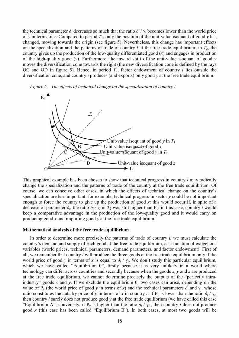
the technical parameter δi decreases so much that the ratio δi / γi becomes lower than the world price of y in terms of x. Compared to period T1, only the position of the unit-value isoquant of good y has changed, moving towards the origin (see figure 5). Nevertheless, this change has important effects on the specialization and the patterns of trade of country i at the free trade equilibrium: in T2, the country gives up the production of the low-quality differentiated good (x) and engages in production of the high-quality good (y). Furthermore, the inward shift of the unit-value isoquant of good y moves the diversification cone towards the right (the new diversification cone is defined by the rays OC and OD in figure 5). Hence, in period T2, factor endowment of country i lies outside the diversification cone, and country i produces (and exports) only good y at the free trade equilibrium.
Figure 5. The effects of technical change on the specialization of country i Ki . .E A Unit-value isoquant of good y in T1 B Unit-value isoquant of good x C Unit-value isoquant of good y in T2 D Unit-value isoquant of good z O Li This graphical example has been chosen to show that technical progress in country i may radically change the specialization and the patterns of trade of the country at the free trade equilibrium. Of course, we can conceive other cases, in which the effects of technical change on the country’s specialization are less important: for example, technical progress in sector y could be not important enough to force the country to give up the production of good x: this would occur if, in spite of a decrease of parameter δi, the ratio δi / γi in T2 was still higher than Py: in this case, country i would keep a comparative advantage in the production of the low-quality good and it would carry on producing good x and importing good y at the free trade equilibrium. Mathematical analysis of the free trade equilibrium
In order to determine more precisely the patterns of trade of country i, we must calculate the country’s demand and supply of each good at the free trade equilibrium, as a function of exogenous variables (world prices, technical parameters, demand parameters, and factor endowment). First of all, we remember that country i will produce the three goods at the free trade equilibrium only if the world price of good y in terms of x is equal to δi / γi. We don’t study this particular equilibrium, which we have called “Equilibrium 0”, firstly because it is very unlikely in a world where technology can differ across countries and secondly because when the goods x, y and z are produced at the free trade equilibrium, we cannot determine precisely the outputs of the “perfectly intra-industry” goods x and y. If we exclude the equilibrium 0, two cases can arise, depending on the value of Py (the world price of good y in terms of x) and the technical parameters δi and γi, whose ratio constitutes the autarky price of y in terms of x in country i. If Py is lower than the ratio δi / γi, then country i surely does not produce good y at the free trade equilibrium (we have called this case “Equilibrium A”; conversely, if Py is higher than the ratio δi / γi , then country i does not produce good x (this case has been called “Equilibrium B”). In both cases, at most two goods will be
19
produced in country i at the free trade equilibrium, so that we can determine precisely the patterns of trade of country i as a function of the exogenous variables.
Study of the Equilibrium A This case arises when Py is lower than the ratio δi / γi. At this relative price, country i doesn’t produce good y at the free trade equilibrium. We assume that the two others goods are produced, so that the zero profit conditions for goods x and z give two equations in two unknowns (prices of factors), hence determining the equilibrium factor prices ratio. The full employment conditions give two equations in two unknowns: outputs of goods x and z. Therefore, substituting the equilibrium factor prices ratio in the full employment conditions, we can determine the supply of goods x and z of country i, as a function of the exogenous variables:
1
1 (1 )( )
S T Ti ii z i z i
i i i
G Gx P K P LG F F
α αβ α β αγ γβ β
β α γ τ τ
− −− −
= − − −
1
1 (1 )( )
S T Ti ii z i z i
i i i
G Gz P L P KF F F
β ββ α β αγ γα α
β α τ τ τ
− −− −
= − − −
Then, substituting the equilibrium factor prices ratio in equations (2.7) and (2.9) and using the zero profit conditions, we can write the demands for goods x and z of country i, as a function of the exogenous variables:
11 ( )T
i yD T Ti ii z i z i
i i i
P G Gx P L P KG F F
α αβ α β αλ ϕ γ γ
γ τ τ
− −− −
− = +
1
1D T Ti ii z i z i
i i i
G Gz P L P KF F F
β ββ α β αγ γλ
τ τ τ
− −− −
− = +
We can now determine for which values of the exogenous variables goods x and z will be produced at the equilibrium (by imposing, respectively, the conditions xi
S > 0 and ziS > 0), and for which
values of the exogenous variables goods x and z will be exported by country i at the equilibrium (by imposing, respectively, the conditions: xi
S - xiD > 0 and zi
S - ziD > 0). In conclusion, we find that the
following patterns of specialization and trade are possible for country i, when Py is lower than the ratio δi / γi
A1) For
1
1 Ti iz
i i
K GPL F
β αγαα τ
− −≥
, country i produces (and exports) only good x. Goods z and y are
imported. Therefore, trade of country i with the rest of the world is partly inter-industry and partly intra-industry.
A2) For
1 1
1 ( )(1 ) 1( )(1 )
T Ti i iz z
i i i
G K GP PF L F
β α β αγ γα β α λ αα β α λ τ α τ
− − − − − − −< < + − − , country i produces goods x
and z; exports only good x; imports goods y and z. Therefore, trade of country i with the rest of the world is still partly inter-industry and partly intra-industry, but the share of inter-industry trade decreases as Ki / Li gets closer to the left term of the inequality.

20
A3) For
1
1 ( )(1 )( )(1 )
Ti iz
i i
K GPL F
β αγα β α λα β α λ τ
− − − − −= + − − , country i still produces goods x and z but its net
demand for good z is equal to zero. Therefore, in this case, trade with the rest of the world is totally intra-industry (exports of x in exchange for imports of y).
A4) For
1 11 ( ) 1 ( ) 1 ( )(1 )
( )(1 )( ) 1 ( )
Ti y T Ti i i
z zTi i ii y
P G K GP PF L FP
β α β αβ β α λ ϕ γ γα β α λτ α β α λ τβ β α λ ϕ
− − − + − − − − − − < < + − − − − − ,
country i produces and exports both goods x and z; imports only good y. Its trade with the rest of the world is once again partly inter-industry and partly intra-industry, but the share of intra-industry trade decreases as Ki / Li gets closer to the left term of the inequality.
A5) For
11 ( ) 1 ( )
( ) 1 ( )
Ti y Ti i
zTi ii y
PK GPL FP
β αβ β α λ ϕ γτβ β α λ ϕ
− − + − − = − − −
, country i still produces goods x and z but
its net demand for good x is equal to zero. Therefore, trade with the rest of the world in this case is totally inter-industry (exports of z for imports of y).
A6) For
1 11 ( ) 1 ( )1
( ) 1 ( )
Ti yT Ti i i
z zTi i ii y
PG K GP PF L FP
β α β αβ β α λ ϕγ γββ τ τβ β α λ ϕ
− − − + − − − < < − − −
, country i still
produces both goods x and z, but it exports only z and imports x and y. Trade is totally inter-industry.
A7) For
1
1 Ti iz
i i
K GPL F
β αγββ τ
− −≤
, country i gives up the production of good x. It produces (and
exports) only good z and it imports goods x and y. Trade remains totally inter-industry. Study of the Equilibrium B This case arises when Py is higher than the ratio δi / γi. At this relative price, country i doesn’t produce good x at the free trade equilibrium. Proceeding as in the study of the equilibrium A, we find that the following patterns of specialization and trade are possible for country i in this case:
B1) For
1
1 Ti iz
Ti y i
K GpL p F
β αδαα τ
− −≥
, country i produces (and exports) only good y. Goods z and x are
imported. Therefore, trade of country i with the rest of the world is partly inter-industry and partly intra-industry.
B2) For
1 1
1 ( )(1 ) 1( )(1 )
T Ti i iz z
T Ty i i y i
G K Gp pp F L p F
β α β αγ γα β α λ αα β α λ τ α τ
− − − − − − −< < + − − , country i produces goods y
and z; exports only good y; imports goods x and z. Therefore, trade of country i with the rest of the world is still partly inter-industry and partly intra-industry, but the share of inter-industry trade decreases as Ki / Li gets closer to the left term of the inequality.
B3) For
1
1 ( )(1 )( )(1 )
Ti iz
Ti y i
K GpL p F
β αγα β α λα β α λ τ
− − − − −= + − − , country i still produces goods y and z but its net
demand for good z is equal to zero. Therefore, in this case, trade with the rest of the world is totally intra-industry (exports of y in exchange for imports of x).

21
B4) For
1 1
1 ( ) ( ) 1 ( )(1 )( )(1 )( ) ( )
T T Ti y i i iz z
T TTy i i y ii y
P G K Gp pp F L p FP
β α β αβ β α λ ϕ γ γα β α λτ α β α λ τβ β α λ ϕ
− − − + − − − − − < < + − − − − , country
i produces and exports both goods y and z; imports only good x. Its trade with the rest of the world is partly inter-industry and partly intra-industry, but the share of intra-industry trade decreases as Ki/Li gets closer to the left term of the inequality.
B5) For
1
1 ( ) ( )
( ) ( )
T Ti yi iz
TTi y ii y
PK GpL p FP
β αβ β α λ ϕ γτβ β α λ ϕ
− − + − = − − , country i still produces goods y and z but its
net demand for good y is equal to zero. Therefore, trade with the rest of the world in this case is totally inter-industry (exports of z for imports of x).
B6) For
1 1
1 ( ) ( )1( ) ( )
TT Ti yi i iz z
T TTy i i y ii y
PG K Gp pp F L p FP
β α β αβ β α λ ϕγ γββ τ τβ β α λ ϕ
− − − + − − < < − − , country i still produces
both goods y and z, but it exports only z and imports x and y. Trade is totally inter-industry.
B7) For
1
1 Ti iz
Ti y i
K GpL p F
β αγββ τ
− −≤
, country i produces (and exports) only good z and it imports
goods x and y. Trade remains totally inter-industry.
5. General equilibrium in free trade: three countries completely specialized
In principle, it would now be possible to move from the analysis of the free trade equilibrium of a small country at given world prices to the study of the general equilibrium of a multi-country world, in which prices are determined endogenously. Unfortunately, even in a two-country world, the general study of such equilibrium proves cumbersome. Furthermore, it would be more interesting to analyse a three-country world, in order to justify theoretically the following stylised fact: high levels of intra-industry trade are observed between similar countries, whereas inter-industry trade prevails between very different countries. That’s for in this section we construct a general equilibrium model of international trade, with three countries, using a strong hypothesis that simplifies the determination of the equilibrium: we assume that the three countries are completely specialized in the production of one good at the free trade equilibrium, and we determine for what values of the exogenous variables (technical parameters, demand parameters and factor endowments) this equilibrium occurs.
Conditions for the complete specialization of the three countries in free trade
We assume that three countries, called 1, 2, and 3, are opened to trade and specialized respectively in the production of goods x, y and z.
According to the results of the previous section, the complete specialization of the three countries constitutes an equilibrium situation if the free trade equilibrium prices respect the following conditions:
2 1
2 1
PTy
δ δγ γ
< < (5.1)
( ) ( )(1 ) (1 )
3 3 1 1
3 3 1 1
1 1P1 1
Tz
K KL L
β α β αα α β βτ τα α α αγ β β γ β β
− −− − − −< < − −
(5.2)

22
( ) ( )(1 ) (1 )
3 3 2 2
3 3 2 2
1 11 1
TzTy
K p KL p L
β α β αα α β βτ τα α α αδ β β δ β β
− −− − − −< < − −
(5.3)
These conditions correspond to those we have defined in the mathematical analysis of the free trade equilibrium, in section 4. To be completely specialized in the production of good x, country 1 must be at the equilibrium A1 as defined in section 4; this condition is stated in the right side of conditions (5.1) and (5.2). To be completely specialized in the production of good y, country 2 must be at the equilibrium B1, and this is affirmed in the left side of condition (5.1) and in the right side of condition (5.3). Finally, to be completely specialized in the production of good z, country 3 must be either at the equilibrium A7 or at the equilibrium B7 (indifferently); this is stated in the left side of conditions (5.2) and (5.3). If the relative prices of goods at the free trade equilibrium are consistent with the three conditions stated above, then the complete specialization of countries 1, 2 and 3 in the production of x, y and z respectively, constitutes an equilibrium situation for the three countries at the same time.
The complete specialization of country 1 and country 2 in the production of, respectively, x and y constitutes an equilibrium in free trade only if condition (5.1) is verified. This condition affirms that the free trade equilibrium price of y in terms of x must be strictly included between the autarky equilibrium price in country 2 (which then specializes in good y) and the autarky equilibrium price in country 1 (which specializes in good x). The autarky equilibrium price of y in terms of x in country i has been determined in section 3, equation (3.4), as the ratio of the technological parameters δi and γi. Therefore, a necessary condition for the complete specialization of country 1 and 2 (respectively in goods x and y) is that country 1 has a relative23 technological advantage in the production of x and country 2 has a relative technological advantage in the production of good y, i.e:
2 1
2 1
δ δγ γ
< (5.4)
The complete specialization of country 1 and country 3 in the production of, respectively, x and z constitutes an equilibrium in free trade only if condition (5.2) is verified. This is possible only if:
( )( )
( )( ) ( )
3 3 1 1
3 3 1 1
11
K KL L
β αβ α β αα βτ τγ β α γ
−− − −
< − (5.5)
We define ( )( )11
Hα ββ α
−= −
. Since we have assumed that β is greater than α, H is always smaller
than one, and condition (5.5) can be restated as follows:
1 1
3 3 1 1
3 3 1 1
K KHL L
β α β ατ τγ γ
− −
<
(5.5)
Condition (5.5) concerns both technology parameters and factor endowments of countries 1 and 3. If we assume for convenience that the technological parameters are identical in countries 1 and
3 (i.e. γ1 = γ3 and τ1 = τ3), condition (5.5) is verified only if country 1 has a capital to labour ratio 23 A relative (and not absolute) technological advantage determines the pattern of the specialization in free trade. Assume for example that technological parameters in the two countries verify the following conditions: δ2 < δ1 ; γ2 < γ1;
2 1
2 1
δ δγ γ
< . In this case, even if country 2 has an absolute technological advantage in the production of both y and x,
complete specialization can occur, because country 1 has a relative advantage in the production of x and country 2 has a relative advantage in the production of y.

23
substantially bigger than country 3. Since H decreases as the difference between β and α increases, the more important is this difference, the bigger must be the difference between the factor endowments ratio in the two countries to permit their complete specialization.
We release now the assumption of identical technology and we come back to the general case allowing for Hicks-neutral differences in the production functions across countries; we can conclude that technological differences contribute to the consistency of the assumption of complete
specialization if 3 1
3 1
τ τγ γ
<
, i.e. if country 1 has a relative technological advantage in the
production of x and symmetrically country 3 has a relative technological advantage in the production of z.
Finally, condition (5.3), which has to be verified to allow the complete specialization of countries 2 and 3 respectively in y and z, can be rewritten as follows:
1 1
3 3 2 2
3 3 2 2
K KHL L
β α β ατ τδ δ
− −
<
(5.6)
As in the previous case, this condition is verified either if the relative endowment of capital of country 2 is substantially bigger than the relative endowment of capital of country 3, or if country 2 has a strong technological (relative) advantage in the production of good y.
In conclusion, the complete specialization of countries 1, 2 and 3, in the production of, respectively, x, y and z constitutes an equilibrium situation in free trade, if:
- countries 1 and 2 have similar ratios of factor endowments and some Hicks-neutral difference in the production functions of x and y;
- country 3 has a capital to labour ratio substantially smaller than countries 1 and 2, or a strong technological disadvantage in the production of x and y.
Determination of the free trade equilibrium prices of goods
If we assume that countries 1, 2 and 3 are respectively specialized in the production of goods x, y and z, the equilibrium conditions of the goods markets in free trade are:
1 2 3 1D D D Sx x x x+ + = (5.7)
1 2 3 2D D D Sy y y y+ + = (5.8)
1 2 3 3D D D Sz z z z+ + = (5.9)
where Dix is the demand of x in country i and S
ix is the production of x of country i. The demand functions of goods x, y and z have been determined in section two24. If we assume that the function φi (Py) is identical in the three countries, equations (5.7), (5.8) and (5.9) can be rewritten as:
( ) (1 )1 1 1 1 2 2 2 2 3 3 3 3 1 1
1
1 (P ) 1Ty
Tx
w L r K w L r K w L r K L Kp
α αλ ϕ
γ−
− + + + + + = (5.7)
( ) (1 )1 1 1 1 2 2 2 2 3 3 3 3 2 2
2
(P ) 1Ty
Ty
w L r K w L r K w L r K L Kp
α αλϕδ
−+ + + + + = (5.8)
24 Cf. equations (2.7), (2.8) and (2.9).

24
( ) (1 )1 1 1 1 2 2 2 2 3 3 3 3 3 3
3
(1 ) 1Tz
w L r K w L r K w L r K L Kp
β βλτ
−− + + + + + = (5.9)
where in the terms on the right we have substituted, respectively, the production function of x in country 1, the production function of y in country 2 and the production function of z in country 3. From equations (5.7) and (5.8), we obtain:
(1 )
2 1 1
1 2 2
1 (P )P
(P )
Ty T
yTy
L KL K
α αϕ δϕ γ
−− =
(5.10)
In order to determine the free trade equilibrium price of y in terms of x, we must give an explicit form to the function φ(Py). Therefore, we assume that the function φ(Py) has the following form, which has been introduced in section two [cf. equation 2.6)]:
1(P ) = if P 1P
(P ) = 1 if P <1
y yy
y y
ϕ
ϕ
≥
Using this form of the function φ(Py), we obtain from equation (5.10) the free trade equilibrium price of y in terms of x:
(1 )
2 1 1(1 )
1 2 2
1 1P2 4
Ty
L KL K
α α
α αδγ
−
−= + + (5.11)
Using equations (5.7) and (5.9) we obtain the free trade equilibrium price of z in terms of x:
(1 )
3 1 1(1 )
1 3 3
P 1PP 1
TyT
z Ty
L KL K
α α
β βτλ
λ γ
−
−
− = − (5.12)
which can be determined also from equations (5.8) and (5.9) as :
( )(1 )2 3 2 2(1 )
2 3 3
1P PT Tz y
L KL K
α α
β βτλ
λ δ
−
−
− =
(5.12)
These are two different and equivalent expressions for the equilibrium price of z in terms of y.
The relative prices (5.11) and (5.12) have been determined by assuming that the three countries are completely specialized. Therefore, they are to be considered as the free trade equilibrium prices only if they satisfy the conditions (5.1), (5.2) and (5.3), because otherwise the complete specialization doesn’t constitute an equilibrium situation for the three countries.
A numerical example of free trade equilibrium of complete specialization
We develop now a numerical example in which the complete specialization of countries 1, 2 and 3 in the production respectively of x, y and z constitutes an equilibrium situation for the three countries in free trade (i.e. the conditions (5.1), (5.2) and (5.3) are verified at the free trade equilibrium). Then we demonstrate that the free trade equilibrium is revealed preferred to autarky equilibrium for the three countries.
In this numerical example, we assume: = 0.3; = 0.7; = 0.5α β λ . These parameters have the same values in the three countries, consistently with the assumptions made in sections one and two.

25
Industry x-y is capital-intensive, while industry z is labour-intensive. The following table defines the values of country-specific technological parameters.
Country 1 Country 2 Country 3
γi 2 2 2δi 4 3 4τi 1 1 1
In order to limit the influence of technological determinants of trade at a minimum necessary, we introduce one only difference in the production functions of the three countries: parameter δ2 is assumed to be smaller than δ1 and δ3, meaning that country 2 has an absolute technological advantage in the production of good y, with respect to countries 1 and 3. Factor endowments in the three countries are:
Country 1 Country 2 Country 3Ki 150 200 50Li 10 10 200
In countries 1 and 2, the ratio of the endowments is not identical but quite similar, characterizing these countries as capital abundant relative to country 3. The equilibrium relative prices of y and z in terms of x and the relative price of factors in autarky and in free trade are shown in the following tables:
Autarky equilibrium prices Country 1 Country 2 Country 3
PAy 2 1.5 2
PAz 1.5749 1.7670 0.3062
(wi / ki)A 17.6087 23.4780 0.2935
Free trade equilibrium prices Country 1 Country 2 Country 3
PTy 1.7151 1.7151 1.7151
PTz 0.9075 0.9075 0.9075
(wi / ki)T 6.4286 8.5714 0.5833
In autarky (cf. section three), good y is cheaper (in terms of x) in country 2 than in the two other countries, whereas good z is cheaper in country 3 than in countries 1 and 2. The price of labour relative to capital is substantially higher in countries 2 and 1 than in country 3.
In free trade, with complete specialization of the three countries (cf. sections four and five), the relative prices of y and z in terms of x are identical in the three countries (for the “One price” law). The equilibrium prices determined with these values of the exogenous variables25 respect the conditions (5.1), (5.2) and (5.3). Therefore, in this numerical example, the complete specialization of countries 1, 2 and 3, respectively in the production of x, y and z, constitutes an equilibrium for the three countries, in free trade. At equilibrium, international trade is partly inter-industry and partly intra-industry in vertically differentiated goods (VIIT), since the bilateral trade between country 3 on the one hand and countries 1 and 2 on the other hand is totally inter-industry, whereas the bilateral trade between country 1 and country 2 is totally VIIT.
25 Equilibrium prices of y and z in terms of x have been calculated using the expressions (5.11) and (5.12).

26
We can observe that, with complete specialization, the relative prices of factors in the three countries are not identical at the free trade equilibrium, so that there is no factor price equalization. Nevertheless, they converge with respect to the autarky equilibrium: in free trade, the price of labour relative to capital is lower than in autarky in the capital-abundant countries, while it is higher than in autarky in the labour-abundant country. By means of the Lerner diagram, we represent now the autarky and the free trade equilibrium situations for the three countries. As it was seen in section 4, the essential feature of the Lerner-Pearce diagram is that it uses unit-value isoquants. In equilibrium, the unit-value isoquants of the goods which are produced in country i are tangent to the unit isocost line in country i, whereas the unit-value isoquants of the goods that are not produced in country i are located above the unit isocost line. We take good x as the numeraire.
Applying the equations of the unit-value isoquants and isocost line introduced in section 4 to this numerical example, we obtain the following graphs for the autarky and the free trade equilibrium in countries 1, 2 and 3. The unit-value isocost line is coloured in black, while the unit-value isoquants are coloured in blue (good x), in brown (good y) and in red (good z).
Equilibrium in Country 1:
Autarky Free Trade
Equilibrium in Country 2:
Autarky Free Trade
z
x,y
0
2
4
6
8
10
K
0.5 1 1.5 2L0
2
4
6
8
10
K
0.5 1 1.5 2L
0
2
4
6
8
10
K
0.5 1 1.5 2L0
2
4
6
8
10
K
0.5 1 1.5 2L
x,y
z
z
z
y x
xy z

27
Equilibrium in Country 3:
Autarky Free Trade
We observe in these figures that in the autarky equilibrium the three goods are produced in each country: in fact, in autarky, the three unit-value isoquants are tangent to the unit isocost line in the three countries26. In free trade, complete specialization constitutes an equilibrium for the three countries, since only one unit-value isoquant is tangent to the isocost line: the blue one for country 1 (which specializes in the production of x), the brown one for country 2 (which specializes in y) and the red one for country 3 (which specializes in z).
It remains to be seen if the free trade equilibrium (with complete specialization) constitutes a better situation than the autarky equilibrium for the three countries. To answer this question, we use revealed preferences: the free trade equilibrium is preferred to the autarky equilibrium if the consumption in free trade, evaluated at autarky prices, is greater than the consumption in autarky.
Using good x as the numeraire, we define and A Ti iC C , respectively, as total consumption in
autarky and in free trade, evaluated at the autarky equilibrium relative prices:
P PA A A A A Ai i iy i iz iC x y z= + +
P PT T A T A Ti i y i z iC x y z= + +
In the following tables, we have calculated, with the particular values of parameters and factor endowments of this numerical example, consumption of goods x, y, and z in the three countries, in autarky and in free trade, and total consumption in terms of the numeraire. We observe from these data that, in the three countries, total consumption in free trade, evaluated at autarky prices, is greater than total consumption in autarky. Thus, we can conclude that free trade equilibrium (with complete specialization) is revealed preferred to autarky equilibrium for the three countries.
26 The blue isoquant (which refers to good x) doesn’t appear in these figures because it coincides with the brown one (which refers to good y).
0
1
2
3
4
5
K
2 4 6 8 10L0
0.5
1
1.5
2
2.5
K
1 2 3 4 5L
x, y
z
y x z

28
Autarky Country 1 Country 2 Country 3Aix 7.4872 6.1050 8.5240Aiy 3.7436 8.1400 4.2620Aiz 14.2620 15.5476 83.5152AiC 37.4361 45.7876 42.6201
Free trade Country 1 Country 2 Country 3
Tix 5.5509 7.7627 19.9703Tiy 4.5261 6.3296 16.2836Tiz 22.0060 30.7744 79.1705TiC 49.2610 71.6354 76.7793
Conclusion In this paper we have presented a theoretical model of international trade which includes
Ricardian and HOS characteristics and we have shown that intra-industry trade in vertically differentiated goods can be explained by technological differences across countries which determine relative advantages in the production of either the high-quality or the low-quality differentiated good.
We have assumed that there are two industries and three goods, called x, y and z. All the goods are produced using two factors (capital and labour) and constant-return-to-scale technologies. Goods x and y are vertically differentiated and belong to the same industry, because they are produced with the same factor intensity at any given factor prices ratio. Good y is assumed to be of a higher quality than good x, so that producing one unit of good y needs more capital and more labour than producing one unit of good x. Good z belongs to another industry, since it has a lower capital intensity than goods x and y. We have introduced Ricardian elements in the HO framework in a very general way, allowing for Hicks-neutral technological differences across countries in all the production functions. Under these assumptions, we have studied the determinants of trade as follows. In the fourth section, we have analysed the free trade equilibrium for a small country opened to international trade. By studying the production possibility surface in our particular case with two vertically differentiated intra-industry goods, we have shown that, in most cases, the country will give up the production of one differentiated good at the free trade equilibrium. What good can be produced (the high-quality one or the low-quality) at given world prices, depends only on relative technological advantage of country i. Using the Lerner diagram, we have represented the possible patterns of specialization for country i at the world trade equilibrium and we have shown that technical progress in country i can potentially change radically the patterns of specialization and trade of the country. Then, we have determined mathematically all the conceivable patterns of specialization and trade for a small country, depending on world prices, technology parameters, demand parameters and factor endowment. Finally, in the last section, we have presented a general equilibrium model with three countries and we have demonstrated that the complete specialization of countries 1, 2 and 3 in the production of goods x, y and z respectively, is a free trade general equilibrium, provided that:
- country 1 and country 2 have similar relative endowments of factors; - countries 1 and 2 are highly capital-abundant with regard to country 3;
29
- there are some (small) Hicks-neutral differences between the production functions of x or y in countries 1 and 2, which generate a relative technological advantage of country 1 in the production of x (and symmetrically a relative advantage of country 2 in the production of y).
If these conditions are satisfied, the complete specialization of the three countries constitutes an equilibrium situation, in which trade between countries 1 and 2 is totally intra-industry, whereas trade between country 3 on the one hand and countries 1 and 2 on the other hand is totally inter-industry.
References Abd-El-Rahman, K. S. (1986), “Réexamen de la définition et de la mesure des échanges croisés de produits similaires entre nations”, Revue Economique, 1: 89-115. Davis, R. D. (1995), “Intra-industry trade: A Heckscher-Ohlin-Ricardo approach”, Journal of International Economics, 39: 201-226. Deardorff, A. (1979), “Weak Links in the Chain of Comparative Advantage”, Journal of International Economics, 9: 197-209. Falvey, R. (1981), “Commercial Policy and Intra-Industry Trade”, Journal of International Economics, 11: 495-511. Feenstra, R. (2004), Advanced International Trade. Theory and Evidence, Princeton University Press, Princeton. Fontagné, L. and M. Freudenberg (2002), “Long-term Trends in Intra-Industry Trade”, in: P. J. Lloyd and Hyun-Hoon Lee eds., Frontiers of Research in Intra-Industry Trade (Palgrave MacMillan, London), 131-158. Greenaway, D. and C. Milner (2002), “Intra-Industry Trade and C-H-O Model: Evidence and Implications for Adjustments”, in: P. J. Lloyd and Hyun-Hoon Lee eds., Frontiers of Research in Intra-Industry Trade, Palgrave MacMillan, London, 180-196. Harrigan, J. (1997), “Technology, Factor Supplies, and International Specialization: Estimating the Neoclassical Model”, The American Economic Review, 87-4: 475-494. Helpman, E. and P. Krugman (1985), Market Structure and Foreign Trade, MIT Press, Cambridge (Mass.). Krugman, P. (1995), “Increasing Returns, Imperfect Competition and the Positive Theory of International Trade", in: G. Grossman and K. Rogoff eds., Handbook of International Economics, vol. III, chapter 24: 1243-1277. Jones, R. (1974), “The Small Country in a Many-Commodity World”, Australian Economic Papers, 13: 225-236. Vanek, J. and T. Bertrand (1971), “Trade and Factor Prices in a Multi-Commodity World”, in: J.N. Bhagwati, R.W. Jones, R.A. Mundell and J. Vanek eds., Trade, balance of payments and growth: Papers in international economics in honour of Charles P. Kindleberger, Elsevier, NY.