A Theoretical Framework for Backward Error Analysis

on Manifolds

Anders C. HansenDAMTP, Centre for Mathematical Sciences

University of CambridgeWilberforce Rd, Cambridge CB3 0WA

United Kingdom

Abstract

Backward Error Analysis (BEA) has been a crucial tool when analyzing long-time behav-ior of numerical integrators, in particular, one is interested in the geometric properties of theperturbed vector field that a numerical integrator generates. In this article we present a newframework for BEA on manifolds. We extend the previously known “exponentially close” es-timates from Rn to smooth manifolds and also provide an abstract theory for classificationsof numerical integrators in terms of their geometric properties. Classification theorems oftype “symplectic integrators generate symplectic perturbed vector fields” are known to betrue in Rn. We present a general theory for proving such theorems on manifolds by lookingat the preservation of smooth k-forms on manifolds by the pull-back of a numerical integra-tor. This theory is related to classification theory of subgroups of diffeomorphisms. We alsolook at other subsets of diffeomorphisms that occur in the classification theory of numericalintegrators. Typically these subsets are anti-fixed points of group homomorphisms.

Dedicated to the memory of Jerrold E. Marsden.

1 Introduction

LetM be a smooth manifold, where, by smooth we throughout the paper mean C∞. A smoothmanifold is presumed to be finite-dimensional, while infinite-dimensional manifolds (when con-sidered in Section 5) will always have the name “infinite”, when addressed. Let X(M) denotethe set of smooth vector fields and let X ∈ X(M). Consider the ordinary differential equation

d

dty(t) = Xy(t), y(t) ∈M. (1.1)

The flow map corresponding to X is denoted by θX : R×M→M. Also, we sometimes use thenotation

θ(q)X (t) = θX,t(q) = θX(t, q),

and if the vector field X is obvious we sometimes use θ instead of θX .A numerical approximation to the solution of (1.1) can be found by constructing a family

of diffeomorphisms Φhh≥0 and then (for each fixed h) one can obtain a sequence qh,nn∈N,often referred to as the numerical solution, satisfying qh,n+1 = Φh(qh,n). We will throughout thepaper denote the family Φhh≥0 by Φh. More formally we have the following:

Definition 1. An integrator is a one-parameter family Φh : M→M of diffeomorphisms thatis smooth in h and satisfies Φ0 = id (the identity mapping). If X ∈ X(M) and

d

dh

∣∣∣h=0

Φh(p) = Xp, p ∈M,

1

then Φh is called an integrator for X. If, for any chart (U,ϕ) onM, there exist a constant C > 0such that, for Φh = ϕ Φh ϕ−1 and sufficiently small h

‖Φh(x)− θY,h(x)‖ ≤ Chp+1, x ∈ ϕ(U),

where Y is the vector field on ϕ(U) induced by ϕ, the integrator Φh is said to be consistent withX of order p.

Remark 1 It follows immediately by smoothness and the Taylor theorem that if Φh is anintegrator for X then Φh is consistent with X of order one.

If Φh is an integrator for the vector field X then, under suitable assumptions on Φh, one canguarantee that there is a metric d on M such that

d(qn, θX,nh(qo)) ≤ Chp, p ∈ N, C > 0,

at least for nh ≤ T for some T > 0 and sufficiently small h. The integer p is often referred to asthe order of the numerical integrator.

The idea of backward error analysis is the following. Supposing that we have a numericalsolution qh,n i.e. qh,n+1 = Φh(qh,n), could it be the case that the sequence qh,n is the“solution” to a different differential equation i.e. does there exist a vector field X ∈ X(M), aperturbation of X, such that

qh,n = θ eX,nh(q0)? (1.2)

If such a vector field exists, one can analyze the flow map θ eX to gain information about thebehavior of qh,n. In most cases (1.2) may not be obtained, and one has to concentrate onconstructing a family of vector fields X(h), depending on the parameter h, such that

d(qh,n, θ eX(h),nh(q0)) ≤ f(h),

where f : R → R is continuous and f(h) → 0 as h → 0. Typically f could be f(h) = Chs forsome C > 0 and s ∈ N. Or even better f(h) = Ce−γ/h for some γ > 0. The construction ofthe family of modified vector fields X(h) and the analysis of the corresponding flow map θ eX(h)

is known as Backward Error Analysis (BEA), and the family X(h) is often referred to as themodified or perturbed vector field.

2 Open problems and novelty of the paper

BEA is very well understood when M = Rn, and modified vector fields X(h) are formallyexpressed as an infinite series

X(h) = X1 + hX2 + h2X3 + . . . , (2.1)

where Xi is uniquely defined by Φh. Thus, it makes sense to talk about the modified (orperturbed) vector field generated by Φh. There are several articles on the subject, Hairer andLubich [9], Calvo, Murua, and Sanz-Serna [4], Benettin and Giorgilli [3] and Reich [19]. Thequestion, however is: what if we are not longer working in Rn but with some abstract manifold,can we still carry out the BEA? To illustrate the idea let us consider a simple example on anabstract manifold, in particular a matrix Lie group G with its corresponding Lie algebra g (forreferences on Lie group problems see [12] and the references therein). Consider the equation

Y ′(t) = AY (t), Y (0) = Y0, A ∈ g, (2.2)

and let Φh be an integrator for the vector field X ∈ X(G) defined by XY = AY. Then, it can beshown (with some appropriate assumptions on Φh, see Chapter IX in [10]) that there exists asequence Ajj∈N ⊂ g such that we can define a vector field X(h) ∈ X(G) by

X(h)Y = (A1 + hA2 + h2A3 + . . .)Y, (2.3)

2

where the series converges in the matrix norm on g. Moreover, if Y is a solution of

Y ′(t) = (A1 + hA2 + h2A3 + . . .)Y (t), Y (0) = Y0,

thenΦnh(Y0) = Y (nh), ∀n ∈ N, Y (t) ∈ G, ∀ t ∈ R+.

There are two important observation and also questions to address:

(i) It is possible to construct a modified vector field whose flow map will interpolate thenumerical solution. However, the convergence in (2.3) is exceptional, and typically in thegeneral case one must truncate a formal series to get a well defined vector field. However,how do we carry out the construction of such a series, and where do we truncate?

(ii) The solution of the modified equation shares a crucial property with the solution to theoriginal problem. Namely, they are both in G. In the general case we may ask the following:if the flow map of the original vector field has a certain property, under which conditionswill the flow map of the modified vector field have the same properties?

The answers to these types of questions are the topic of this paper.

2.1 Extending estimates from Rn to manifolds

In the papers of Benettin and Giorgilli [3] , Hairer and Lubich [9] and Reich [19] the questionof closeness of the numerical solution and the solution to the modified equation is addressed. Inparticular, it has been shown that for a suitable truncation of the series (2.1)

‖θ eX(h),h(q)− Φh(q)‖ ≤ Che−γ/h, q ∈ K, (2.4)

where C,γ > 0 and K ⊂ Rn is compact. A crucial assumption for the previous estimate to betrue is that both the vector field and the integrator Φh are analytic. In [9] Hairer and Lubichtake (2.4) even further and show that (with some extra assumptions) variants of (2.4) are trueeven for multiple steps (not just one as (2.4) indicates). This ia a very powerful result as itsuggests that the numerical solution is close to the true solution of the modified equation. Thisis all great, but what if Rn is replaced by a smooth manifold M?

First, we are faced with the problem of constructing modified vector fields (as in (2.1))on the manifold. This has been done by Reich in [18], Hairer, Lubich, Wanner in [10] andHairer [8]. Although the techniques are different, they yield the same result. The techniqueused in [18] is based an the assumption that M is embedded in Rn, and by using a tubularneighborhood technique, one extends the original vector field and integrator to a neighborhoodaround the manifold. By applying the standard technique from Rn to the extended vector fieldand integrator, one obtains the modified vector field on the manifold M. The approach in [8] issimilar, however, one assumes that the vector field is already defined on a neighborhood of themanifold. Hairer et al. [10] have a different strategy where the construction is done via chartsand no extension of the vectorfield is needed.

Second, with the modified vector field established, do results of type (2.4) automatically follow(with the norm substituted by a metric of course)? (Note that this question is not addressedin [18, 10, 8]). This is a delicate question. It is tempting to try to use the already establishedtechniques in Rn, and typically for the long time estimates, the results of Hairer and Lubich [9].However, to do so we must transform our problem to Rn. One way to do this would be to followthe idea of Reich, via the tubular neighborhood, to obtain an extended vector field and integratoron a neighborhood of the manifoldM. Although tempting, this approach has a serious obstacle.Note that analyticity is crucial for results a la (2.4). The problem is that the mappings used inthe extension approach are only C∞, and hence analyticity is lost. Discouraged by that fact, onemay try to emulate the ideas of Hairer et al. What if we simply use charts and do the analysislocally in Rn? This would work because, by assuming that the manifold is analytic, the chartswould be analytic. However, it is not enough to use charts and just quote the results by Hairerand Lubich [9] and deduce long term estimates on the manifold. The problem is that analysisin charts will only be local. To illustrate this issue we have chosen the following example:

3

Example 2.1. Let M = S2 ⊂ R3, where S2 denotes the two sphere in R3. This is a compactmanifold that can be given an analytic structure, however, it cannot be covered by only one chart.Suppose that we have an analytic vector field X on S2 and that Φh is an analytic integratorfor X with corresponding modified vector field X(h) (to simplify the notation we will use thenotation X). Let qnn∈Z+ denote the numerical solution (e.g. qn+1 = Φh(qn)). Suppose thatour task is to show that there is a metric d on S2 and constants C, γ > 0 such that

d(θ eX,nh(q0), qn) ≤ Ce−γ/h, (2.5)

however, we insist on using local charts and the techniques from Hairer and Lubich [9] directly(in those charts). We start by finding a chart (U,ϕ) such that q0 ∈ U. Now suppose that qn ∈ Ufor n ≤ K for some K > 0. Now let Φh : ϕ(U)→ ϕ(U) be defined by Φh = ϕ Φh ϕ−1, and letY and Y be the vector fields on ϕ(U) induced by ϕ and X and X respectively, e.g. Y = ϕ∗X

and Y = ϕ∗X (see Section 3 for notation). Suppose that we have been able to show (using thevector space techniques in [9]) the existence of C, γ > 0 such that

‖θeY ,nh(q0)− qn‖R2 ≤ Ce−γ/h, n ≤ K, (2.6)

(where qn = ϕ(qn)) however, for N = K + 1 then qK+1 /∈ U. This forces us to change charts. Sosuppose that we can find a chart (V, ψ) such that qK ∈ U∩V and qn ∈ V for K ≤ n ≤ L for someL > K. Let Φh, Z and Z be induced by (V, ψ) and Φh, X, X (similarly as above). To continuethe analysis we first need to establish a bound on ‖θeZ,Kh(q0)− qK‖R2 (where qn = ψ(qn)). Theonly way we can do that is to use the already established (2.6). In particular, we have

‖θeZ,Kh(q0)− qK‖R2 = ‖ψ ϕ−1(θeY ,Kh(q0))− ψ ϕ−1(qK)‖R2 ,

however, to be able to use (2.6) we must establish that ψ ϕ−1 is Lipschitz continuous and abound on the Lipschitz constant, say Cψϕ−1 . By invoking (2.6) we then get

‖θeZ,Kh(q0)− qK‖R2 ≤ Cψϕ−1Ce−γ/h.

The problem now is that when continuing the analysis in the chart (V, ψ) we must take intoaccount the accumulated error from the previous chart that depends on Cψϕ−1 (and of coursethis constant may be greater than one). In fact, every time we would have to change chartswe would get a contribution from the Lipschitz constant of the composite mapping. As weare interested in long term behavior we cannot restrict ourselves to the assumption that thenumerical solution only changes charts finitely many times. And if we cannot do that, the typeof analysis suggested in this example would yield estimates a la (2.5), however, with a constant Cthat grows every time the numerical solution changes chart. Such a result would be substantiallyless than optimal.

This leaves us with the following open question. How do we extend results a la (2.4) tomanifolds? This question (and the answer) is one of the main themes of this paper. As we willsee, abstractions of the ideas by Hairer and Lubich [9] and Reich [19, 18] will be crucial.

2.2 Extending classification theory from Rn to manifolds

A very important question to ask is: when will the flow map of the modified vector field have thesame geometric properties as the original flow map? A typical question of this type would be:will the flow map of the modified vector field be symplectic provided that the original flow mapis symplectic? The answer is yes, if the integrator is symplectic. Several other results regardinggeometric properties of modified vector field can be found in [7], [10]. However, all these resultsare so far only valid when considering ODEs in Rn, and we may therefore ask the same questionas before: What if Rn is replaced by a manifold M. There are some results in [10], however,these techniques work only for quite specific cases and are not suited for the general problemsthat we will consider here.

4

Now consider a very basic example. Let ρ : M → M be a diffeomorphism on a smoothmanifold M and denote the mapping

Ψ 7→ ρ Ψ ρ−1, Ψ ∈ Diff(M),

by σ. Note that this is a homomorphism on Diff(M) (the set of diffeomorphisms on M, a morethorough definition follows below) since σ(Ψ Φ) = σ(Ψ) σ(Φ), for Ψ,Φ ∈ Diff(M). Supposethat X ∈ X(M) is a vector field with flow map θX,t with the property that

σ(θX,t) = θ−1X,t = θX,−t. (2.7)

Suppose that we have an integrator Φh for X and that Φh satisfies σ(Φh) = Φ−1h . The question

is then: Will the flow map θ eX(h),t of the modified vector field X(h) satisfy

σ(θ eX(h),t) = θ−1eX(h),t= θ eX(h),−t? (2.8)

This has been considered in the Rn case when ρ(x) = Tx, x ∈ Rn and T is a linear operator in[7] and [19]. However, even the simplest case whenM is a sphere and T is a unitary involution isnot covered by the theory in [7] and [19]. One can off course ask a more general question: whatif σ simply is a homomorphism such that (2.7) is satisfied? Would (2.8) follow? The existingtheory is quite far from covering such a general question, even in Rn, and of course not in thegeneral setting.

Consider another basic example. Let µ be a volume form on a smooth manifold M andsuppose that X ∈ X(M) is a vector field whose flow map θX,t satisfy

θ∗X,tµ = µ,

(the notation θ∗X,t denotes the standard pull back). Given an integrator Φh for X with theproperty that Φ∗hµ = µ. Does it follow that the flow map θ eX(h),t of the modified vector field

X(h) satisfyθ∗eX(h),t

µ = µ?

This question has been investigated in [7] and [19], however, only in the Rn case, and even thesimplest example of a sphere will not be covered by the existing theory. The examples aboveare just two basic examples of what is not covered by the existing theory, and, in fact, there is aquite long list of open questions: Let X ∈ X(M), with flow map θX,t, for some smooth manifoldM. Suppose that Φh is an integrator for X with corresponding modified vector field X(h) andflow map θ eX(h),t.

(i) Let ω be a symplectic 2-form on M. Suppose θX,t,Φh ∈ S1 = ϕ ∈ Diff(M) : ϕ∗ω = ω.Does it follow that θ eX(h),t ∈ S1?

(ii) Let ω be a symplectic 2-form on M. Suppose θX,t,Φh ∈ S2 = ϕ ∈ Diff(M) : ϕ∗ω =cω , c ∈ R. Does it follow that θ eX(h),t ∈ S2?

(iii) Let µ be a volume form on M. Suppose θX,t,Φh ∈ S3 = ϕ ∈ Diff(M) : ϕ∗µ = µ. Doesit follow that θ eX(h),t ∈ S3?

(iv) Let µ be a volume form onM. Suppose θX,t,Φh ∈ S4 = ϕ ∈ Diff(M) : ϕ∗µ = cµ , c ∈ R.Does it follow that θ eX(h),t ∈ S4?

(v) Let α be a contact form. Suppose θX,t,Φh ∈ S5 = ϕ ∈ Diff(M) : (ϕ∗α)p = cϕ(p)αp , cϕ ∈C∞(M). Does it follow that θ eX(h),t ∈ S5?

(vi) Let f ∈ C∞(M). Suppose θX,t,Φh ∈ S6 = ϕ ∈ Diff(M) : f ϕ = f. Does it follow thatθ eX(h),t ∈ S6?

5

(vii) Let σ : Diff(M)→ Diff(M) be a homomorphism. Suppose θX,t,Φh ∈ S7 = ϕ ∈ Diff(M) :σ(ϕ) = ϕ−1. Does it follow that θ eX(h),t ∈ S7?

It seems to be a dearth of literature on these basic questions and we therefore consider it animportant task to develop an abstract framework that can handle these issues. Before embarkingon such a challenge let us ask the question: Can we build this on the existing frameworks?The novel ideas by Reich [19] are of a very abstract nature and are well suited for furtherdevelopments. It is the notion of the “Tangent Space at the Identity” of Diff(M) that is thecrucial tool that can be used in an abstract framework . As we will see in Example 6.2 andRemark 5 the framework in [19] is not complete, even in Rn, however, it can be completed andmade abstract. In order to do the abstraction we feel it is natural to go to the source of suchtechniques, namely, the work by Ebin and Marsden [6] on infinite-dimensional manifolds, inparticular, infinite-dimensional subgroups of Diff(M). Our framework is very much inspired bytheir work.

The theory in this paper may seem involved at first glance, and it may be appropriate toask: are such technical abstractions really necessary? A question like that must be viewed in thelight of the questions we are asking. Note that the questions in (i)-(vii) above are very general,in particular (vii). As in most cases in mathematics, general questions may have to be treatedwith abstract framework (that may happen to be involved). To answer the initial question, theanswer is yes, as the Remark 7 shows.

3 Background and notation

We will first introduce some notation. If M and N are smooth manifolds and F : M → N isa smooth map, we will adopt the notation from [13] and denote the derivative, or the tangentmapping TpF : TpM → TpN , by F∗ e.g. for x ∈ TpM we let F∗x = TpFx. The derivative ofa function F : Rn → Rm will be denoted by DF, and similarly derivatives of higher order willbe denoted by DrF. As usual we identify DrF (x) with Lrsym(Rn,Rm), the set of symmetric rlinear mappings from Rn × · · · × Rn (r-times) to Rm. The set of smooth k-forms on M will bedenoted by Ωk(M).

Given a vector field X with corresponding flow map θX : I ×M →M, where I is an openinterval of R, we will allow slight misuse of notation by letting θX(t, s, p) denote the flow of Xat time t that takes the value p at time s. We also adopt the Einstein summation convention,meaning that

∑i x

iEi will be denoted by xiEi, hence omitting the summation sign.Throughout this section M = Rn and we will review some of the well known results that

will be crucial for our developments in the upcoming sections. Let Φh be an integrator on Rn,and suppose that Φh is consistent of order p with X ∈ X(Rn). As discussed in the introduction,the idea is to look for a family of vector fields X(h) such that Φh ≈ θ eX(h),h and thus the studyof the numerical solution reduces to the study of the flow θ eX(h). The family of modified vector

fields X(h) is formally defined in terms of an asymptotic expansion in the step size h; i.e.,

X(h) = X1 + hX2 + h2X3 + . . .

The infinite sequence of vector fields Xii=1,...,∞ can be obtained by using the Taylor seriesexpansion of the one-step method Φh i.e.,

Φh = id+ hΦ1 + h2Φ2 + . . . ,

where id is the identity map and the Φjs are smooth mappings, and then compare this serieswith the expansion of the flow map θh, eX(h). The vector fields Xi are chosen such that these twoseries coincide term by term. We will follow the recursive approach by Reich [19] when definingthe vector fields Xi, as this approach is advantageous when one wants to study the geometricproperties of the modified vector field as done in Section 5.

6

The recursive construction is as follows. Let Φh be an integrator for the smooth vector fieldX. Suppose that we have obtained Xjij=1, and we want to determine Xi+1. Let

Yi(h) =i∑

j=1

hj−1Xj .

Suppose that Xjij=1 has been chosen such that the distance between Φh(q) and θh,Yi(h)(q) isO(hi+1) for all q ∈ Rn. Now define

Yi+1(h) = Yi(h) + hiXi+1, Xi+1(q) = limh→0

Φh(q)− θh,Yi(h)(q)hi+1

, q ∈ Rn. (3.1)

Note that the limit exists by the choice of Yi(h). This definition of Yi+1(h) generates a flow mapthat is O(hi+2) away from Φh. Indeed, by Taylor’s theorem and the definition of Yi+1(h) we get

θh,Yi+1(h)(q)− θh,Yi(h)(q) = hi+1Xi+1(q) +O(hi+2)

andθh,Yi(h)(q)− Φh(q) = hi+1Xi+1(q) +O(hi+2).

Thus,

θh,Yi+1(h)(q)− Φh(q) = θh,Yi(h)(q) + hi+1Xi+1(q)− Φh(q) +O(hi+2)

= O(hi+2).(3.2)

Letting X1 = X the construction is complete. Note that it is easy to see that Xi = 0 fori = 2, . . . , p when Φh is of order p.

As mentioned above there are several important results regarding BEA in Rn, and for anexcellent review we refer to [10]. Some of the results in [19] are of crucial importance for thefollowing arguments and we will give a short summary. Let Br(x) ⊂ Cn be the open complexball of radius r around x ∈ Rn. Let also ‖ · ‖ denote the max norm on Cn. Let K ⊂ Rn be acompact subset and define, for Z ∈ X(Rn) and r > 0 ,

‖Z‖r = supx∈BrK

‖Zx‖, where BrK =⋃x0∈K

Br(x0).

Lemma 3.1. (Reich) Let Φh be an integrator for X ∈ X(Rn). Suppose that the vector field Xis real analytic in an open set U ⊂ Rn and that there is a compact subset K ⊂ U and constantsK, R > 0 such that ‖X‖R ≤ K. Suppose also that the mapping h 7→ Φh(x) is real analytic forall x ∈ U . Then there exist M ≥ K such that

‖Φτ − id‖αR ≤ |τ |M ≤ (1− α)R for |τ | ≤ (1− α)RM

,

where α ∈ [0, 1).

Theorem 3.2. (Reich) Let the assumptions of Lemma 3.1 be satisfied and let Φh be consistentof order p with X . Then, the family Xi defined in (3.1) is analytic and, for all integersm ≥ p+ 1, there exists C > 0, such that, for X(h)m = X1 + hX2 + h2X3 + . . .+ hm−1Xm, wehave

supx∈K‖Φh(x)− θ eXm,h

(x)‖ ≤ Ch(h(m− p+ 1)M

R

)m,

where Xj is defined as in (3.1). Also,

supx∈K‖Xj(x)‖ ≤ C

((j − p)M

R

)j−1

, j ≥ p+ 1.

Remark 2 Note that Theorem 3.2 is not quoted directly as stated in [19], but the boundspresented here come from equation (4.17) and (4.13) in the proof of Theorem 2 in [19]. Notethat the results in Lemma 3.1 and Theorem 3.2 are stated in Rn, however, they will be usefulin the proofs below as we will use these estimates in local coordinates.

7

4 Backward error analysis on manifolds

This section is devoted to answering the questions posed in Section 2.1. The following theoremis a generalization of Theorem 2 in [19] and Theorem 1 in [9].

Theorem 4.1. Let M be a smooth manifold, X ∈ X(M) and let Φh be an integrator that isconsistent with X of order p. Then there exists a family of smooth vector fields Xjj∈N on M,where each Xj is uniquely determined by Φh, with the following properties:

(i) There is a metric d on M such that if K ⊂ M is a compact subset and for any N ∈ Nsuch that XN (h) = X1 + hX2 + . . . hN−1XN there exists a CN > 0, depending on N, suchthat for sufficiently small h > 0 we have

d(θ eXN ,h(q),Φh(q)) ≤ CNhN+1, q ∈ K,

where θ eXNis the flow map of XN (h).

(ii) IfM, X are analytic and h 7→ Φh(q) is analytic for q in compact K ⊂M, then there existsan integer k (depending on h) and C, γ > 0 such that for X(h) = X1 + hX2 + . . . hk−1Xk

it follows that, for sufficiently small h,

d(Φh(q), θ eX,h(q)) ≤ Che−γ/h, (4.1)

for all q ∈ K, where d is the same metric as in (i). Also, there exists a finite collection Fof charts on M, covering K, and a constant C > 0 such that if (U,ϕ) ∈ F and Y , Y (h)are the vector field induced by ϕ and X, X(h) respectively then

supx∈ϕ(U)

‖Y (x)− Y (h)(x)‖ ≤ Chp, supx∈ϕ(U)

‖DY (x)−DY (h)(x)‖ ≤ Chp. (4.2)

Proof. The construction of Xj is as follows: For any chart (U,ϕ), let Φh = ϕ Φh ϕ−1 andlet Y be the vector field induced by ϕ. Doing the calculations in (3.1) and (3.2) with Φh and θYwe obtain a family of smooth vector fields Yj on ϕ(U), and hence also a family ϕ−1

∗ Yj on U.It is easy to see, using the fact that Yj is uniquely defined by Φh, that ϕ−1

∗ Yj is independentof the choice of charts. Thus, we obtain a family of global smooth vector fields Xj from thelocal construction. Also, each Xj is uniquely determined by Φh. (This construction can also befound in Theorem 5.1 Chap. IX.5 in [10]).

To show (i), note that, by compactness of K, consistency of Φh and the fact that θX,0 = Φ0 =id, we can find a finite collection F = (Uj , ϕj) of charts such that there are open sets Vj ⊂ Ujand h0 > 0, such that θX,h(Vj) ⊂ Uj and Φh(Vj) ⊂ Uj , for h < h0 (for some h0 > 0) and Vjcovers K. We may also assume without loss of generality that ϕ−1

j is defined on ϕj(Uj).To get the desired metric and bound that we asserted, we use the Whitney Embedding

Theorem to obtain a diffeomorphism F : M → N ⊂ Rm for some m ≥ 2n, where N is anembedded submanifold and n = dim(M). By the choice of F above we have that if p ∈ K thenq = ϕ(p) for some (U,ϕ) ∈ F , and, by letting XN = X0 + hX1 + . . . hNXN and by a littlemanipulation and the calculation in (3.1) and (3.2), we get that

‖F Φh(p)− F θ eXN ,h(p)‖ = ‖F ϕ−1(Φh(q))− F ϕ−1(θYN ,h

(q))‖ ≤ CNhN (4.3)

where CN bounds the Lipschitz’s constant of all F ϕ−1 and YN (h) = Y +hY1 + . . . hNYN . Notethat F ϕ−1 is Lipschitz by smoothness and since ϕ(U) is compact and can be assumed withoutloss of generality to be convex. Also, since N is embedded, it has the subspace topology andhence it inherits a metric from Rm which again leads to a metric d on M induced by F .

To show (ii), notice that we may, by arguing as in the proof of (i) and possibly changing F ,where F is as in the proof of (i), assume that for each (U,ϕ) ∈ F there is an rϕ > 0 such thatBrϕ

(0) is properly contained in ϕ(U),

θX,h(ϕ−1(Brϕ(0))) ⊂ U, Φh(ϕ−1(Brϕ

(0))) ⊂ U, h ≤ h0,

8

and⋃

(U,ϕ)∈F ϕ−1(Brϕ

(0)) is an open cover of K. Let (U,ϕ) ∈ F and let Y be the induced vector

field on V = ϕ(U) of X by ϕ, and let K = Brϕ(0). From the previous discussion it follows that

there exists an Rϕ > 0 such that the complexification of Y is defined on BRϕK and by continuity

‖Y ‖Rϕ ≤ Kϕ for some Kϕ > 0. Now consider the integrator on V defined by Φh = ϕ Φh ϕ−1.We can now apply Lemma 3.1 and Theorem 3.2 to obtain constants Mϕ, Cϕ > 0 such that

Ym = Y1 + hY2 + h2Y3 + . . .+ hm−1Ym, m ≥ p+ 1,

where Yj is the vector field on ϕ(U) induced by Xj and ϕ. We have the estimates

‖Φh(x)− θYm,h(x)‖ ≤ Cϕh

(h(m− p+ 1)Mϕ

Rϕ

)m, x ∈ K, (4.4)

‖Yj(x)‖ ≤ Cϕ(

(j − p)Mϕ

Rϕ

)j−1

, x ∈ K, j ≥ p+ 1. (4.5)

To get the metric and the desired bounds, let

M = maxMϕ : ϕ ∈ F, C = maxCϕ : ϕ ∈ F, R = minRϕ : ϕ ∈ F.

To show (4.1), we can now use the same approach as in (i) and apply (4.4) to get

d(Φh(q), θ eXm,h(q)) ≤ Ch

(h(m− p+ 1)MR

)m, q ∈ K,

where C is a constant depending on C and the Lipchitz constants of F ϕ−1. (F is here as in theproof of (i)). To get the desired bound we choose m to be the integer part of µ = R

hMe + p− 1.Hence, we get

d(Φh(q), θ eXm,h(q)) ≤ Che−m

≤ Che−µ+1

≤ Che−pe−γ/h, q ∈ K,

where γ = R/(Me).To show (4.2), note that by analyticity and Cauchy’s integral formula, it follows by (4.5) (by

possibly changing C) that

max (‖Yj(x)‖, ‖DYj(x)‖) ≤ C(

(j − p)MR

)j−1

, x ∈ K, j ≥ p+ 1.

Thus, since Φh is of order p

max(‖Yj(x)− Yj(h)(x)‖,‖DYj(x)−DYj(h)(x)‖)

≤ Cm∑

j=p+1

(hM(j − p)

R

)j−1

= C

(hM

R

)p m∑j=p+1

(j − p)p(hM(j − p)

R

)j−1−p

≤ C(hM

R

)p m∑j=p+1

(j − p)p

ej−p−1

(j − p

m− p+ 1

)j−1−p

≤ C(hM

R

)pdpK,

(4.6)

where dp bounds (j−p)p

ej−p−1 and K bounds∑mj=p+1

(j−p

m−p+1

)j−1−p. Also, in the second to last

inequality we have used the fact that

h ≤ R

Me(m− p+ 1).

The theorem follows.

9

Remark 3 The computation in (4.6) is almost word for word taken from the last computationsin the proof of Theorem 2 in [19].

The idea is now to use this result and follow the ideas in the proof of Corollary 2 (p. 444) in[9] applied to a general manifold setting. This corollary is using Lady Widermere’s fan, andthat technique requires vector space operations. Hence, unfortunately, the corollary cannot beapplied directly, but after a series of preparations we can follow the analysis in [9] closely.

Let us first recall some basic facts from differential geometry that will be useful in thefollowing argument. By the normal space to an embedded submanifold M⊂ Rn at x we meanthe subspace NxM⊂ TRn consisting of all vectors that are orthogonal to TxM with respect tothe Euclidean dot product. The normal bundle of M is the subset NM⊂ TRn defined by

NM =∐x∈M

NxM = (x, v) ∈ TRn : x ∈M, v ∈ NxM.

Define a map E : NM→ Rn byE(x, v) = x+ v, (4.7)

where we have done the usual identification. A tubular neighborhood of M is a neighborhoodU of M in Rn that is the diffeomorphic image under E of an open subset V ⊂ NM of the form

V = (x, v) ∈ NM : |v| < δ(x)

for some positive continuous function δ :M→ R. A useful fact that will come in handy in thenext theorem is that every embedded submanifold of Rn has a tubular neighborhood.

Theorem 4.2. LetM be a smooth manifold and X ∈ X(M) with flow map θX that exists for allt ∈ R and all p ∈M. Let Φh be an integrator that is consistent of order r with X. Let qh,nn∈Z+

be the numerical solution produced by Φh recursively and let Xi be the family of vector fieldsfrom Theorem 4.1. Suppose that there is a compact set K ⊂ M, h0 > 0 and T ≤ ∞ such thatqh,nn≤T/h ⊂ K for all h ≤ h0. For any integer s ≥ r + 1, let X(h) = X1 + hX2 + . . . hs−1Xs.Suppose also that ⋃

t≤T,h≤h0,s<∞

θ eX(h),t(qh,nn≤T/h) ⊂ K, (4.8)

and that for any finite collection F of charts covering K then θX,t has uniformly bounded spacialderivatives for all |t| ≤ T in any charts belonging to F . (To simplify notation we will simplydenote qh,n by qn.)

(i) Then there are constants L > 0 and Cs > 0 (depending on s) such that

d(θ eX(h),nh(q0), qn) ≤ hs+1Cs

(eLh

r+1n − 1eLhr+1 − 1

), nh ≤ T.

(ii) If M, X and h 7→ Φh(p) are analytic and X(h) is as in (ii) of Theorem 4.1, then thereexist constants L > 0 and C > 0 such that

d(θ eX,nh(q0), qn) ≤ he−γ/hC

(eLh

r+1n − 1eLhr+1 − 1

), nh ≤ T.

Proof. We will show that there are constants C > 0 and L > 0 such that

d(θ eX,t(p), θ eX,t(q)) ≤ CeLhrtd(p, q), t ≤ T, p, q ∈ qh,nn≤T/h, (4.9)

where d is the same metric as in Theorem 4.1. Now, suppose for the moment that (4.9) is true.Recall that qh,nn∈Z+ is the numerical solution obtained recursively by Φh and let tk = kh.

10

Also, to avoid cluttered notation we will use just X for X(h). Then

d(θ eX,tn(q0), qn) ≤n∑k=1

d(θ eX(tn, tk−1, qk−1), θ eX(tn, tk, qk))

≤n∑k=1

CeLhr(tn−tk)d(θ eX(tk, tk−1, qk−1), θ eX(tk, tk, qk))

=n∑k=1

CeLhr(tn−tk)d(θ eX,h(qk−1), qk),

where the second inequality follows from (4.9) and the last equality follows from the fact thatθ eX(tk, tk, qk) = qk and θ eX(tk, tk−1, qk−1) = θ eX,h(qk−1). Thus, using Theorem 4.1, we get thetwo cases

(i) d(θ eX,tn(q0), qn) ≤ C1hs+1

∑n−1k=0 e

Lhrkh = hs+1C1

(eLhr+1n−1

eLhr+1−1

),

(ii) d(θ eX,tn(q0), qn) ≤ C2he−γ/h∑n−1

k=0 eLhrkh = C2he

−γ/h(eLhr+1n−1

eLhr+1−1

),

where C1 and C2 are the constants from Theorem 4.1 (i) and (ii) respectively. Also, the lastinequalities in cases (i) and (ii) come from the standard techniques used to prove convergenceof one step methods (details can be found on p. 161 [11]). Thus, to conclude, we only need toshow (4.9). To do that we will transform our problem from the manifold setting into a vectorspace environment and then follow the analysis in Corollary 2 [9] quite closely.

By Whitney’s embedding theorem we obtain a smooth embedding F :M→ Rm, for m ≥ 2n,where n = dim(M). Let N = F (M). Now, F, X and X induce vector fields on N , namely,F∗XF−1(·) and F∗XF−1(·). With a slight misuse of notation we will also denote these vectorfields by X and X respectively. Our first goal is to extend X and X to a neighborhood aroundN .

Let U be a tubular neighborhood of N i.e. N ⊂ U ⊂ Rm where U is open in Rm anddiffeomorphic to an open set V ⊂ NN of the form

V = (x, v) ∈ NN : |v| < δ(x) (4.10)

for some positive continuous function δ : N → R. Note that diffeomorphism mentioned aboveE : V → U is defined as in (4.7). For (x, v) ∈ NN we identify T(x,v)NN with TxN ×Rm−n anddefine the vector fields Z and Z by

Z(x,v) = (Xx, 0) ∈ TxN × Rm−n, Z(x,v) = (Xx, 0) ∈ TxN × Rm−n. (4.11)

Now Z and Z are obviously smooth, thus, we can define smooth vector fields Y and Y on U byY = E∗ZE−1(·) and Y = E∗ZE−1(·). We are now in the position where we can apply the ideasfrom the proof of Corollary 2 [9]. But before we do so we need to establish two facts.

Claim I. There exists a smooth vector field Y on U such that Y − Y = hrY . Indeed, by theconstruction of X, and the fact that Φh is of order r, it follows that there is a vector field X onN such that

X = h−r(X − X). (4.12)

Thus, for x ∈ U, we have

Yx − Yx = E∗(ZE−1(x) − ZE−1(x))

= E∗

((Xπ(E−1(x)), 0)− (Xπ(E−1(x)), 0)

)= hrE∗(Xπ(E−1(x)), 0),

(4.13)

where π : NN → N is the canonical projection. Thus, by letting Y = E∗(ZE−1(·)− ZE−1(·)) theassertion follows.

11

Claim II. There is a compact set K ⊃ F (K) such that the interior Ko ⊃ F (K) is open in U,and there is a constant M > 0 such that (independently of h) we have

supz∈eK

∥∥∥Y (z)∥∥∥ ≤M, sup

z∈eK∥∥∥DY (z)

∥∥∥ ≤M, (4.14)

supz∈eK

∥∥∥∥ ∂∂z θY (t, s, z)∥∥∥∥ ≤M, sup

z∈eK∥∥∥∥ ∂2

∂z2θY (t, s, z)

∥∥∥∥ ≤M, s < t ≤ T. (4.15)

Let F be the collection of charts referred to in Theorem 4.1 (ii). It is easy to see that we maywithout loss of generality assume that F is a family of charts on N , covering F (K), with theproperties stated in Theorem 4.1 (ii). Now, for (V, ϕ) ∈ F , define Uϕ = x ∈ U : π(E−1(x)) ∈V , where π : NN → N is the canonical projection. Observe that Uϕ is obviously open in Rmand also

F (K) ⊂⋃

(V,ϕ)∈F

Uϕ

(this is clear by the definition of E). Let K be a compact set with the properties that Ko is openin Rm and

F (K) ⊂ Ko ⊂ K ⊂⋃

(V,ϕ)∈F

Uϕ.

Note that (4.15) follows immediately from the assumption about uniformly bounded spacialderivatives of θX,t in any charts belonging to F . To see (4.14), for (V, ϕ) ∈ F let Fϕ : Uϕ×Rn →Rm be defined by

Fϕ(x, v) = TE−1(x)E · (Taϕ−1 · v, 0), a = ϕ π(E−1(x)),

whereTE−1(x)E : Tπ(E−1(x))N × Rm−n → Rm

and A · y denotes that the operator A acts linearly on y. Then by (4.13) we get

Yx − Yx = hrFϕ(x, Xϕ(ρ(x))), ρ(x) = ϕ π(E−1(x)), x ∈ Uϕ,

where Xϕ is the vector field on ϕ(V ) induced by X and ϕ, (X is defined in (4.12)). Hence,

D(Y−Y )(x) · y

= hrDFϕ(x, Xϕ(ρ(x))) · (y,DXϕ(ρ(x)) ·Dρ(x) · y), x ∈ Uϕ, y ∈ Rm.

By Theorem 4.1 (ii) it follows that there is a constant K such that

supy∈ϕ(V )

‖Xϕ(y)‖ ≤ K, supy∈ϕ(V )

‖DXϕ(y)‖ ≤ K,

uniformly for all sufficiently small h and all ϕ ∈ F . This allows us to find a constant bounding‖DFϕ(x, Xϕ(ρ(x)))‖, ‖DXϕ(ρ(x))‖ and ‖Dρ(x)‖ for all x ∈ Uϕ and ϕ ∈ F . Since Uϕϕ∈Fcovers K we, deduce that ‖DY (x)‖ is bounded uniformly for all sufficiently small h and for allx ∈ K. Similar reasoning gives a bound on ‖Y (x)‖ for small h and all x ∈ K.

Note that we may without loss of generality assume that K is convex. Indeed, if that isnot the case choose a compact set K whose interior is open and an open set U such thatF (K) ⊂ Ko ⊂ K ⊂ U ⊂ K, and an f ∈ C∞(Rm) such that 0 ≤ f(x) ≤ 1, supp(f) ⊂ U and f

is equal to one on K. Define Yf = fY, Yf = fY and Yf = fY . Now Claim I and Claim II arestill valid (possibly with different constants) for these vector fields and since they are globallydefined K could be chosen to be convex.

Now, using Claim I and the Alekseev-Grobner formula (p. 96, [11]) (recall that θX(t, s, p)denotes the flow of X at time t that takes the value p at time s, see Section 3) we get, forp ∈ F (qh,nn≤T/h), that

θ(p)eY (t) = θ

(p)Y (t) + hr

∫ t

0

∂

∂zθY (t, s, θ(p)eY (s))Y (θ(p)eY (s)) ds, t ≤ T.

12

Note that the latter expression is justified by the assumption on global existence of θX and (4.8).Hence, by using the above expression also for q ∈ F (qh,nn≤T/h), subtracting the two equationsand applying Claim II (this is where convexity is crucial) it follows that

‖θ(p)eY (t)− θ(q)eY (t)‖ ≤M‖p− q‖+ hr∫ t

0

2M2‖θ(p)eY (t)− θ(q)eY (t)‖, t ≤ T.

Letting L = 2M2 and by appealing to the Gronwall lemma [11] gives

‖θ(p)eY (t)− θ(q)eY (t)‖ ≤ CeLhrt‖p− q‖, t ≤ T.

Hence, since M inherits a metric from N similarly to what is done in the proof of Theorem 4.1we obtain (4.9), and we are done.

5 Geometry in infinite dimensions

Given an integrator Φh, Theorem 4.1 and Theorem 4.2 assures us that there is a unique familyof vector fields Xi such that for some properly chosen N, the vector field XN (h) = X1 +hX2 +. . .+hN−1XN will have a flow map θ eXN (h),t that is close to the integrator (in the sense describedin Theorem 4.1 and Theorem 4.2). Thus it makes sense to talk about the perturbed or modifiedvector field induced by Φh. In the following we will refer to XN (h) as the perturbed or modifiedvector field and to simplify the notation we will denote the perturbed vector field by X(h). Itis of great importance in order to understand the behavior of the numerical approximation thatwe understand the behavior of θ eX(h),t. A convenient tool for analyzing θ eX(h),t is the theory ofclassifications of diffeomorphisms.

Definition 2. Let M be a smooth manifold. Define

Diff(M) = ϕ ∈ C∞(M,M) : ϕ is a bijection, ϕ−1 ∈ C∞(M,M).

In the following we will consider subsets of Diff(M) with certain geometric properties. Weare interested in determining under which conditions geometric properties of the flow map ofthe original vector field will be preserved by the flow map of the perturbed vector field. In otherwords, if the flow map θX,t of a vector field X is in some subset S ⊂ Diff(M), under whichconditions will θ eX(h),t ∈ S? To answer the previous question it is convenient to look at Diff(M)as a manifold itself, in particular as an infinite dimensional manifold.

5.1 Cartan’s subgroups

Diffeomorphism groups and subgroups occur frequently in classical mechanics and are thereforea crucial concept in Geometric Integration. The theory of such groups originate, from the workof Lie and Cartan [5], in particular Cartan gave a classification of the complex primitive infinite-dimensional diffeomorphism groups, finding six classes. We will give a brief review here and referto [14] for a more detailed discussion. The diffeomorphism groups of Cartan are as follows:

• Diff(M), the group of all diffeomorphisms on M.

• The diffeomorphisms preserving a symplectic 2-form ω onM, that is the set of diffeomor-phisms ϕ such that ϕ∗ω = ω.

• The diffeomorphisms preserving a volume form µ onM, that is the set of diffeomorphismsϕ such that ϕ∗µ = µ.

• The diffeomorphisms preserving a given contact 1-form α up to a scalar function, that isthe set of diffeomorphisms ϕ such that (ϕ∗α)p = cϕ(p)µ.

• The group of diffeomorphisms preserving a given symplectic form ω up to an arbitraryconstant multiple, that is the set of diffeomorphisms ϕ such that ϕ∗ω = cϕω.

13

• The group of diffeomorphisms preserving a given volume form µ up to an arbitrary constantmultiple, that is the set of diffeomorphisms ϕ such that ϕ∗µ = cϕµ.

These subgroups serve as a motivation for most of the theory in the upcoming sections.

5.2 Infinite-dimensional manifolds

We will give a short review of the basic definitions of infinite-dimensional manifolds, their tangentbundle and tangent spaces. For a more thorough treatment of the subject we refer to [15]. Foran informal introduction of the concept of vector fields belonging to some Lie algebra generatedby a group of diffeomorphisms we refer to [2].

Definition 3. A Hausdorff space M is called a C∞-manifold modeled on a separable locallyconvex topological vector space E if M is covered by an indexed family Uα : α ∈ A of opensubsets of M satisfying the following:

(i) For each Uα, there is an open subset Vα ⊂ E and a homeomorphism ϕα : Vα → Uα.

(ii) If Uα∩Uβ 6= ∅ then ϕ−1β ϕα is a C∞ diffeomorphism of ϕ−1

α (Uα∩Uβ) onto ϕ−1β (Uα∩Uβ).

The maps ϕ−1β ϕα are called coordinate transformations.

(iii) The indexed family A is the maximal one among indexed families satisfying (i) and (ii)above.

M is called a Frechet, Banach or Hilbert manifold if E itself is a Frechet, Banach or Hilbertspace respectively.

Throughout the paper we will use the name E-manifold to describe a C∞-manifold modeledon a separable locally convex topological vector space E. With a smooth structure on M wecan define the tangent bundle and the tangent space. First we need to introduce an equivalencerelation.

Definition 4. Let M be an E-manifold. Let x ∈ Vα and y ∈ Vβ . Then x and y are equivalent(x ∼ y) if and only if x and y are contained in the domains of ϕ−1

β ϕα, ϕ−1α ϕβ and ϕ−1

β ϕα(x) =y.

Now, for an infinite-dimensional manifold M covered by Uα = ϕ−1α (Vα) : α ∈ A we may

view M as Vα : α ∈ A glued together with the equivalence relation from Definition 4. Thisgives rise to the following definition of the tangent bundle and the tangent space.

Definition 5. The tangent bundle TM of an E-manifold M is the collection Vα×E : α ∈ Aglued according to the following equivalence relation:

(x, u) ∈ Vα × E and (y, v) ∈ Vβ × E

are equivalent if and only if x ∼ y and (ϕ−1β ϕα)∗u = v.

Definition 6. Define the mapping π of⋃α∈A Vα × E onto

⋃α∈A Vα by π(x, u) = x. Since

(x, u) ∼ (y, v) yields π(x, u) = π(y, v), then π naturally defines a mapping (which we will, byslight abuse of notation, denote by the same symbol) π of TM onto M. This map is called theprojection of the tangent bundle. Then the tangent space of M at p is defined as

TpM = π−1(p).

5.3 The smooth structure of Ck(M), Hs(M) and Diff(M)

Before we define Ck(M) and Hs(M) and show how to make them into manifolds, we needto discuss how to make Banach and Hilbert spaces out of sections of vector bundles. We willfollow [16] (Chap. IV) quite closely. Firstly, we need to define an inner product and norm on

14

Lksym(Rn,Rm). Let ej be an orthonormal basis for Rn and define, for T, S ∈ Lksym(Rn,Rm),the inner product and norm

〈T, S〉 = 〈T (ei1 , . . . , eik), S(ei1 , . . . , eik)〉, ‖T‖ = 〈T, T 〉1/2.

(Recall the Einstein summation convention here (discussed in Section 3). In particular, theabove inner product is a sum over all indices). Secondly, let M be a compact manifold and letπ : E →M be a smooth vector bundle over M of rank m. Now, for smooth f : N →M, whereN is a smooth manifold, we let π′ : f∗E → N denote the pull back bundle and Γ(E) denote theset of all smooth sections of E.

We can now make subspaces of Γ(E) into Banach and Hilbert spaces. Let Γ(Bn,Rm) denotethe vector space of all functions from the closed n-ball Bn ⊂ Rn with radius one into Rm, regardedas the set of sections of the product bundle Bn ×Rm over Bn. Now cover M with finitely manycharts (Ui, ϕi)ri=1 such that ϕi(Ui) = Bn, and choose trivializations Ψi on (ϕ−1

i )∗E such thatΨi : π′−1(Bn)→ Bn × Rm. Define the linear mapping

F : Γ(E)→r⊕i=1

Γ(Bn,Rm), F (ξ) = (ξ1, . . . ξr), ξi(x) = Ψi(ξ ϕ−1i (x)) (5.1)

and define the norm ‖·‖B,k and inner product 〈·, ·〉H,k in the following way. For u = (u1, . . . , ur), v =(v1, . . . , vr) ∈

⊕ri=1 Γ(Bn,Rm), let

|u|B,k = max1≤j≤k

r∑i=1

supx∈Bn

‖Djui(x)‖

〈u, v〉k = max1≤j≤k

r∑i=1

∫Bn

〈Djui(x), Djvi(x)〉 dx,(5.2)

and for ξ, η ∈ Γ(E)

‖ξ‖B,k = |F (s)|B,k, 〈ξ, η〉H,k = 〈F (ξ), F (η)〉k.

Let Ck(E) = Γ(E) and Hs(E) = Γ(E), where the closures are in the norms ‖ · ‖B,k and ‖ · ‖H,srespectively. These Banach and Hilbert spaces will be useful in the next developments.

Given two smooth manifolds, M and N , let Ck(M,N ) denote the set of mappings from Mto N such that their derivatives (in any local coordinates) of order ≤ k exist and are continuous.Also, if s > dim(M)/2 we let Hs(M,N ) denote the set of mappings from M to N with squareintegrable (in charts) derivatives (in the distributional sense) of order ≤ s. We will show how tomake Ck(M) and Hs(M) (where Ck(M) and Hs(M) are short for Ck(M,M) and Hs(M,M))into a Banach and Hilbert manifold respectively. The description will be rather brief and werefer to [6] and [15] for a more detailed discussion.

First one needs candidates for the charts on Ck(M). Let f ∈ Ck(M) and define

TfCk(M) = g ∈ Ck(M, TM) : π g = f,

where π : TM→M is the canonical projection. Note that TfCk(M) can naturally be identifiedwith Ck(f∗(TM)) with the norm as discussed above, and hence we have the desired Banachspace. Similar reasoning applies to Hs(M) by replacing Ck(f∗(TM)) with Hs(f∗(TM)).

As we will only need a chart around the identity in the following arguments, we will showhow to construct the chart for f = id and refer to [6] [15] [20] for the general case. Let expqdenote the Riemannian exponential map expq : TqM→M (note that expq is defined on all ofTqM since M is compact). Define Exp : TM→M×M, by

Exp(vq) = (q, expq(vq)).

Now Exp is a diffeomorphism from a neighborhood N (M×0) of M×0 ⊂ TM (where wehave allowed a minor misuse of notation usingM×0) to a neighborhood U(∆) of the diagonal∆ ⊂M×M. This defines a neighborhood V(id) around id, namely,

V(id) = f ∈ Ck(M) : Gr(f) ⊂ U(∆), (5.3)

15

where Gr(f) is the graph of f. Similarly, we define a neighborhood W(ζ0) of the zero sectionζ0 :M→ TM by

W(ζ0) = X ∈ TidCk(M) : X(M) ⊂ N (M×0)

We can now define the chart (ωExp,V(id)) by

ωExp(f) = Exp−1 (id, f), f ∈ V(id),

ω−1Exp(X) = Pr2 Exp X, X ∈ W(ζ0),

(5.4)

where Pr2 :M×M→M is the projection onto the second factor.Using this differentiable structure, Ck(M) becomes a Banach manifold [6], [15] and similarly

we can make a Hilbert manifold of Hs(M). The brief discussion above can be summarized inthe following theorem [20].

Theorem 5.1. LetM be a compact Riemannian manifold. Then, with the differential structuresuggested above, Ck(M), where k ≥ 1, and Hs(M), where s > dim(M)/2, become Banach andHilbert manifolds respectively. Also

TidCk(M) = Xk(M), TidH

s(M) = XsH(M),

where Xk(M) denotes the set of vector fields whose derivatives (in local coordinates) of order ≤ kexist and are continuous, and XsH(M) denotes the set of vector fields such that the derivatives(in the distributional sense) of order ≤ s in local coordinates exist and are square integrable.

Actually, the differentiable structure suggested above is independent of the choice of Rie-mannian metric on M, however, that fact will not be central in the upcoming discussions.Throughout this paper Ck(M) and Hs(M) are understood to have the differential structure aspresented above. The following property of integrators, stated in Theorem 5.2, is quite conve-nient and will be a crucial ingredient in some of the later sections. The key is really that for anintegrator Φh on a smooth compact manifold M, there is a difference between the mappings

R 3 h 7→ Φh ∈ Ck(M), R 3 h 7→ Φh(q) ∈M, q ∈M. (5.5)

And of course there is a difference between the derivatives

d

dh

∣∣∣h=0

Φh ∈ Xk(M),d

dh

∣∣∣h=0

Φh(q) ∈ TqM. (5.6)

Note that it is not clear that the properties of an integrator are sufficient for the existence ofthe derivative in the first part of (5.6), and this must be established. Also, if the derivativeexist, even though the mappings in (5.5) are different, could it be true that for q ∈ M we have(ddh

∣∣h=0

Φh)

(q) = ddh

∣∣h=0

Φh(q)?

Theorem 5.2. Let M be a compact n dimensional manifold and let Φh be an integrator on M.Then there exist neighborhoods U ⊂ Ck(M) and U ⊂ Hs(M) of id (the identity), where k ≥ 1and s > n/2, such that the mappings R 3 h 7→ Φh ∈ U and R 3 h 7→ Φh ∈ U are smooth forsufficiently small h. Also,(

d

dh

∣∣∣h=0

Φh

)(q) =

d

dh

∣∣∣h=0

Φh(q), q ∈M.

Proof. We will first establish the existence of U and then prove that h 7→ Φh ∈ U is smooth.Note that by the reasoning in Section 5.3 there is a neighborhood U ⊂ Ck(M), containing theidentity, defined by

U = f ∈ Ck(M) : Gr(f) ∈ U(∆),

where U(∆) is defined as in (5.3), such that (V, ωExp) is a local chart around id, and ωExp isdefined in (5.4). We claim that Φh ∈ U for all sufficiently small h. Indeed, this is true, forsince U(∆) is a neighborhood of the diagonal ∆ ∈ M×M (in the product topology), and by

16

compactness of M, it suffices to show that for r, s > 0 and q ∈ M, there is an h0 such thatΦh(Br(q)) ⊂ Br+s(q) for h < h0, where Br(q) denotes the open ball of radius r around q withrespect to some metric d onM. Let X ∈ X(M) be defined by Xp = d

dh

∣∣h=0

Φh(p). Then there isa h0 > 0 such that

θX,h(Br(q)) ⊂ Br+s(q), h ≤ h0. (5.7)

Now, since Φ : R×M→M is smooth, and by the classical convergence analysis of integratorsin Rn and compactness of M, it follows that there is a C > 0 such that d(θX,h(q),Φh(q)) ≤ Ch(where d is the metric on M) for h ≤ h for some h > 0. Thus, using (5.7), the assertion follows.

Consider the smooth mapping ωExp Φ : R×M→ TM as a time-dependent smooth vectorfield. Choose charts (Ui, ϕi) and trivializations Ψi and define F as in (5.1). To prove thath 7→ Φh is differentiable, we need to show that there is a vector field Y ∈ X(M) such that

limt→0

1t|F (ωExp Φ)(h+ t, ·)− F (ωExp Φ)(h, ·)− tF (Y )|B,k = 0,

where | · |B,k is defined as in (5.2), and

limt→0

1t|F (ωExp Φ)(h+ t, ·)− F (ωExp Φ)(h, ·)− tF (Y )|s = 0,

where | · |s is the norm induced by 〈·, ·〉s defined in (5.2). We claim that he vector field definedby Yp = d

du

∣∣u=h

(ωExp Φ)(u, p) is the right candidate (obviously Y ∈ X(M)). Letting ξi be alocal representative of ωExp Φ with respect to Ψi and ϕi as in (5.1), it suffices to show that

limt→0

max0≤l≤k

supx∈Bn

1t‖Dlξi(h+ t, x)−Dlξi(h, x)− tDl d

du

∣∣∣u=h

ξi(u, x)‖ = 0 (5.8)

and

limt→0

max0≤l≤s

1t

∫Bn

⟨Dlξi(h+ t, x)−Dlξi(h, x)− tDl d

du

∣∣∣u=h

ξi(u, x),

Dlξi(h+ t, x)−Dlξi(h, x)− tDl d

du

∣∣∣u=h

ξi(u, x)⟩dx = 0.

(5.9)

To see (5.8), let t = (t, 0, . . . , 0) and let D denote the total derivative on the space C1(Rn+1, Rn)Then, by Taylor’s Theorem [1] and smoothness of ξi it follows that

ξi(h+ t, x)− ξi(h, x)− t ddu

∣∣∣u=h

ξi(u, x)

= ξi(h+ t, x)− ξi(h, x)− Dξi(h, x)(t)

= D2ξi(h, x)(t, t) +R(h, x, t)(t, t),

where both D2ξi and R are smooth. Hence

limt→0

max0≤l≤k

supx∈Bn

1t‖DlD2ξi(h, x)(t, t) +DlR(h, x, t)(t, t)‖ = 0,

where DlD2ξi(h, x)(t, t) and DlR(h, x, t)(t, t) and are the l-th derivatives of

x 7→ D2ξi(h, x)(t, t) and x 7→ R(h, x, t)(t, t)

respectively, and we have shown (5.8). Now, (5.9) follows by similar reasoning. To show thath 7→ Φh is infinitely smooth we observe that ωExp Φ is infinitely smooth and since Yp =ddu

∣∣u=h

(ωExp Φ)(u, p) we may argue as above using Taylor’s theorem and deduce smoothness.We are now done with the first part of the proof. Since we have established above that for q ∈Mwe have (

d

dh

∣∣∣h=0

Φh

)(q) =

d

dh

∣∣∣h=0

(ωExp Φ)(h, q),

17

the last assertion of the theorem is straightforward, as seen by the following calculation(d

dh

∣∣∣h=0

Φh

)(q) =

d

dh

∣∣∣h=0

(ωExp Φ)(h, q)

=d

dh

∣∣∣h=0

exp−1q (Φh(q))

= (exp−1q )∗

d

dh

∣∣∣h=0

Φh(q)

=d

dh

∣∣∣h=0

Φh(q).

Let D1(M) be the set of C1 diffeomorphisms onM (a compact manifold) and let Diffs(M) =D1(M) ∩Hs(M), for s > dim(M)/2 + 1, Then Diffs(M) is open in Hs(M) ([6] p. 107) and

Diffs(M) = ψ ∈ Hs(M) : ψ is bijective, ψ−1 ∈ Hs(M). (5.10)

Since Diffs(M) is an open subset of Hs(M), it naturally inherits its smooth manifold structurefrom Hs(M). Throughout the paper Diffs(M) will denote the set in (5.10) with this smoothstructure. We immediately get the following.

Corollary 5.3. Let M be a compact manifold and let Φh be an integrator on M. Then thereexists a neighborhood U ⊂ Diffs(M), where s > dim(M)/2 + 1, such that the mapping R 3 h 7→Φh ∈ U is smooth for sufficiently small h and(

d

dh

∣∣∣h=0

Φh

)(q) =

d

dh

∣∣∣h=0

Φh(q), q ∈M.

Proof. Follows immediately from Theorem 5.2

The next theorem describes the smoothness of the group operations: multiplication andinvertion on Diffs(M).

Theorem 5.4. [20] For s > dim(M)/2 + 1 it follows that Diffs(M) is a smooth infinite-dimensional manifold and a Lie group in the following sense: For g ∈ Diffs(M), right multipli-cation is C∞ as a map

Rg : Diffs(M)→ Diffs(M), Rg(f) = f g.

Left multiplication is Ck as a map

Lg : Diffs+k(M)→ Diffs(M), Lg(f) = g f.

The group multiplication µ is Ck as a map

µ : Diffs+k(M)×Diffs(M)→ Diffs(M), µ(f, g) = f g.

The inversion ν is Ck as a map

ν : Diffs+k(M)→ Diffs(M), ν(f) = f−1.

5.4 Alternative definition of the tangent space at the identity

Similarly to the discussion in the previous section one may consider submanifolds of Diffs(M).We thus consider a symplectic 2-form on M and let

S = ϕ ∈ Diffs(M) : ϕ∗ω = ω. (5.11)

18

Then, according to [6], if s > 12dim(M) + 1 then S is a closed submanifold of Diffs(M) and

TidS = X ∈ XsH(M) : LXω = 0, (5.12)

where LXω denotes the Lie derivative of ω with respect to X.Returning to Cartans subgroups of Diff(M), we are interested in determining the tangent

spaces at the identity for these subgroups of Diff(M). But not only that, we will see in theupcoming discussion that there are subsets of Diff(M) without group structure that may be ofinterest in geometric integration. The problem we are faced with when focusing on finding TidSfor some subset S ⊂ Diff(M), is that, to be rigorous (according to Definition 6), we must imposea smooth structure on S. This can be quite technical and sometimes may be impossible. Notethat the crucial assumption in defining a smooth structure on Diffs(M) has been compactnessof M, and this is an assumption we would like to remove. Also, we are interested in veryspecific subsets of Diff(M), namely subsets of one-parameter diffeomorphisms (integrators andflow maps).

Our goal is therefore to find a definition of the tangent space at the identity of subsets ofintegrators and flow maps that is independent of the choice of smooth structure on the set, andalso coincides with the usual definition on well-known examples. Note that by our definitionof integrator, it is superfluous to talk about integrators and flow maps, as a flow map is anintegrator.

Suppose that we should choose a heuristically and more intuitive definition of the tangentspace at the identity of (5.11) to obtain (5.12). A natural definition would be to consider thecollection of derivatives at zero of smooth curves R 3 t 7→ f(t) ∈ S, where f(0) = id i.e.

TidS = X ∈ X(M) : X =d

dt

∣∣∣t=0

f(t), f(t) ∈ S, f(0) = id.

Thus, if we consider the set S ⊂ S defined by S = Φh ∈ S : Φh is an integrator, a naturaldefinition of the tangent space at the identity of S is

TidS = X ∈ X(M) : X =d

dt

∣∣∣h=0

Φh, Φh ∈ S,

where ddt

∣∣h=0

Φh would have been well defined by Corollary 5.3 had we considered the smoothstructure discussed in Section 5.3. But this definition is based on an underlying smooth structureon S since the derivative d

dt

∣∣h=0

Φh is defined as the derivative of the mapping h 7→ Φh ∈ S. Toget rid of that extra technicality we suggest the following

TidS = X ∈ X(M) : Xq =d

dh

∣∣∣h=0

Φh(q), Φh ∈ S, q ∈M.

This definition does not depend on any smooth structure on S, it only depends on the smoothstructure on M as we take the derivative of the mapping h 7→ Φh(q) ∈M.

Note that it is not clear that with the latter definition that TidS = X ∈ X(M) : LXω = 0,(even though that is the case, see Section 6) but if we consider the following subset of S, namely,S = θt ∈ S : θt is a flow map, then obviously, by the formula for the Lie derivative

TidS = X ∈ X(M) : LXω = 0.

Thus our definition is compatible with (5.11) and (5.12). To be more formal, by the reasoningabove, we suggest the following definition.

Definition 7. Let S ⊂ Diff(M) be a set of integrators. Define the tangent space at the identityby

TidS = X ∈ X(M) : Xq =d

dh

∣∣∣h=0

Φh(q), Φt ∈ S, q ∈M.

Note that the idea of defining the tangent space at the identity in this way was first (at leastto our knowledge) introduced by Reich in [19] for M = Rn. The requirement that M = Rn

19

is irrelevant for the definition, however, and Reich should be credited for introducing such animportant tool. Note also that the name “tangent space” used here is a slight abuse of languageas there is no restriction on S and therefore TidS may not be a vector space e.g. considerS = Φh containing only one element. Then the vector field X defined by Xq = d

dt

∣∣h=0

Φh(q)is in TidS but tX, for t ∈ R, may not be in TidS as Φh may not be a flow map.

Remark 4 Note that if A = TidS there may exist S such that S 6= S and A = TidS. Considerthe following short argument. Let M = Rn and let ω be a symplectic 2-form on M. LetA = X ∈ X(M) : LXω = 0 and

S = θt ∈ Diff(M) : θ∗tω = ω, θt is a flow map.

Then A = TidS. Let X ∈ A and let the integrator Φh be Euler’s method applied to X and letS = S ∪ Φh. By consistency we have d

dh

∣∣h=0

Φh(x) = Xx. Hence TidS = A.

Throughout the paper we will be concerned with the question: Given S ⊂ Diff(M) andX ∈ TidS will the flow map θX,t ∈ S. Note that this obviously not automatic as S may containonly one element that is not a flow map (only an integrator). It is therefore important toestablish conditions on S such that the answer to the question above is affirmative. We will firstdefine a notion of closedness of S that does not depend on any smooth structure (and topology)of Diff(M) (it only depends of the topology on M).

Definition 8. Let S ⊂ Diff(M) be a semi group. Then S is said to be closed iff for anyintegrator Φh ⊂ S, then

Ψh(p) = limn→∞

Φh/n · · · Φh/n(p), (n times) p ∈M,

exists and Ψh ∈ S.

Proposition 5.5. Let S ⊂ Diff(M) be a semi group. Then S is closed iff for every X ∈ TidSthen the flow map θX,t ∈ S.

Proof. Let X ∈ X(M) be the vector field generated by Φh (i.e. Xp = ddh

∣∣h=0

Φh(p)). Note thatif M = Rn, it follows by the standard convergence proof of one-step methods [11] that

Ψh(p) = limn→∞

Φh/n · · · Φh/n(p), (n times) p ∈M, (5.13)

exists and also Ψh = θX,h (the flow map of X). To extend this result to a smooth manifold wemay use exactly the same embedding technique from the proof of Theorem 4.2 via the tubularneighborhood as in (4.10) and eventually define a vector field as in (4.11) and then apply theresult in (5.13). We omit the details, however, conclude that (5.13) is valid for arbitrary smoothmanifolds. Note that since (5.13) is valid regardless of any assumptions on the closedness of S,the assertion of the proposition follows.

6 Classification theory of integrators

In the following we will assume that X ∈ A ⊂ X(M) where A is a vector subspace of theinfinite-dimensional Lie algebra of vector fields onM. In addition we will assume that there is aclosed semigroup S ⊂ Diff(M) such that A = TidS. We will show that if the integrator Φh ∈ Sthen the perturbed vector field X(h) ∈ A.

Theorem 6.1. Suppose that X ∈ A ⊂ X(M) where A is a linear subspace. Let S ⊂ Diff(M)be a semigroup that is closed in the sense of Definition 8 such that A = TidS. Suppose also thatthe integrator Φh ∈ S for all h. Then the perturbed vector field X(h) ∈ A and the flow map θ eX,hof X(h) is also in S.

20

Proof. Let Xj be the family of vector fields from Theorem 4.1. It suffices to show that Xj ∈ Afor all j ∈ N. We do so by induction. Suppose that Xj ∈ A for i ≤ j. We will show that Xj+1 ∈ A.To to that we need to show that there is a one-parameter family of diffeomorphisms Ψh ∈ Ssuch that, for p ∈M, we have Xj+1(p) = d

dh

∣∣h=0

Ψh(p). Let Xj = X1 +hX2 + . . .+hj−1Xj . Weclaim that

Ψh = θ−1eXj ,h1/(1+j) Φh1/(1+j)

is the right candidate. Note that it is not clear (because of the root) that Ψh is smooth at h = 0,but that is part of the proof. However, Ψh ∈ S, indeed, by the induction assumption and theassumption that A is a vector space we have θ−1eXj ,t

= θ− eXj ,t∈ S, so since Φh ∈ S and by the

semigroup hypothesis the assertion follows. Let (U,ϕ) be a chart on M, and let Yj and Yjbe the vector fields induced by ϕ, Xj and Xj. By the construction of Xj it suffices to showthat d

dh

∣∣h=0

Ψh(x) = Yj+1(x), where Ψh is a local representative of Ψh with respect to ϕ, andx ∈ ϕ(U). To see this, note that by the construction of Xj and Taylor’s theorem it followsthat

Φh(x) = θeYj ,h(x) + hj+1Yj+1(x) + hj+2Z(x, h),

where Φh is the local representative of Φh with respect to ϕ and Z is some smooth mapping.This gives, again by Taylor’s theorem, that there is a smooth mapping R : Rn×Rn → L2

sym(Rn)such that

θ−1eYj ,h Φh(x) = θ−1eYj ,h

(θeYj ,h(x) + hj+1Yj+1(x) + hj+2Z(x, h))

= x+Dθ−1eYj ,h(x)W (x, h) +D2θ−1eYj ,h

(x)(W (x, h),W (x, h))

+R(θeYj ,h(x),W (x, h))(W (x, h),W (x, h)),

(6.1)

where W (x, h) = hj+1Yj+1(x) + hj+2Z(x, h). It is easy to see (by smoothness) that

‖D2θ−1eYj ,h(x)(W (x, h),W (x, h))

+R(θeYj ,h(x),W (x, h))(W (x, h),W (x, h))‖ = O(hj+2), h→ 0.

And also, since θ−1eYj ,his a flow map, it follows that Dθ−1eYj ,h

(x) = I +O(h) as h→ 0. Hence

θ−1eYj ,h Φh(x) = x+ hj+1Yj+1(x) +O(hj+2), h→ 0.

Hence,

Yj+1(x) = limh→0

θ−1eYj ,h1/(1+j) Φh1/(1+j)(x)− x

h=

d

dh

∣∣∣h=0

Ψh(x).

The fact that X1 = X ∈ A completes the induction and we are done.

In a later section we will treat the case where S is not a subgroup, but has some otherstructure. However, a natural question to ask is: does S have to have any structure at all? Theanswer is affirmative as the following example shows.

Example 6.2. We follow the reasoning in Remark 4 and let ω be a symplectic 2-form onM = Rn. Also, we have the subspace A = X ∈ X(M) : LXω = 0 and

S = θt ∈ Diff(M) : θ∗tω = ω, θt is a flow map.

Then A = TidS. If X ∈ A and Φh is Euler’s method (forward Euler) applied to X and we letS = S ∪ Φh then

d

dh

∣∣∣h=0

Φh(x) = Xx and TidS = A.

Thus, if we relax the semigroup hypothesis in Theorem 6.1 and assume no structure on the set,then S is a set and TidS = A so, if Theorem 6.1 was true without the semigroup assumption,the perturbed vector field of Euler’s method would be symplectic. It is easy to find examples ofsymplectic vector fields such that the perturbed vector field of Euler’s method is not symplecticand thus we have a contradiction.

21

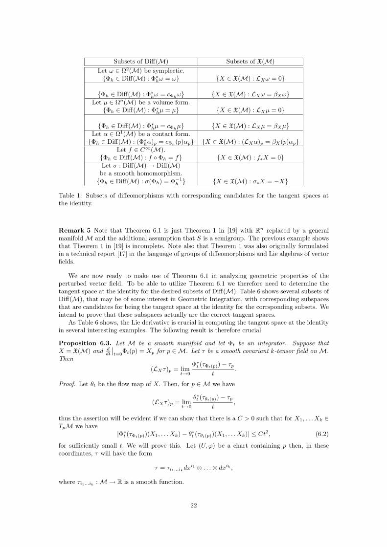
Subsets of Diff(M) Subsets of X(M)Let ω ∈ Ω2(M) be symplectic.Φh ∈ Diff(M) : Φ∗hω = ω X ∈ X(M) : LXω = 0

Φh ∈ Diff(M) : Φ∗hω = cΦhω X ∈ X(M) : LXω = βXω

Let µ ∈ Ωn(M) be a volume form.Φh ∈ Diff(M) : Φ∗hµ = µ X ∈ X(M) : LXµ = 0

Φh ∈ Diff(M) : Φ∗hµ = cΦhµ X ∈ X(M) : LXµ = βXµ

Let α ∈ Ω1(M) be a contact form.Φh ∈ Diff(M) : (Φ∗hα)p = cΦh

(p)αp X ∈ X(M) : (LXα)p = βX(p)αpLet f ∈ C∞(M).

Φh ∈ Diff(M) : f Φh = f X ∈ X(M) : f∗X = 0Let σ : Diff(M)→ Diff(M)

be a smooth homomorphism.Φh ∈ Diff(M) : σ(Φh) = Φ−1

h X ∈ X(M) : σ∗X = −X

Table 1: Subsets of diffeomorphisms with corresponding candidates for the tangent spaces atthe identity.

Remark 5 Note that Theorem 6.1 is just Theorem 1 in [19] with Rn replaced by a generalmanifoldM and the additional assumption that S is a semigroup. The previous example showsthat Theorem 1 in [19] is incomplete. Note also that Theorem 1 was also originally formulatedin a technical report [17] in the language of groups of diffeomorphisms and Lie algebras of vectorfields.

We are now ready to make use of Theorem 6.1 in analyzing geometric properties of theperturbed vector field. To be able to utilize Theorem 6.1 we therefore need to determine thetangent space at the identity for the desired subsets of Diff(M). Table 6 shows several subsets ofDiff(M), that may be of some interest in Geometric Integration, with corresponding subspacesthat are candidates for being the tangent space at the identity for the corrsponding subsets. Weintend to prove that these subspaces actually are the correct tangent spaces.

As Table 6 shows, the Lie derivative is crucial in computing the tangent space at the identityin several interesting examples. The following result is therefore crucial

Proposition 6.3. Let M be a smooth manifold and let Φt be an integrator. Suppose thatX = X(M) and d

dt

∣∣t=0

Φt(p) = Xp for p ∈M. Let τ be a smooth covariant k-tensor field on M.Then

(LXτ)p = limt→0

Φ∗t (τΦt(p))− τpt

.

Proof. Let θt be the flow map of X. Then, for p ∈M we have

(LXτ)p = limt→0

θ∗t (τθt(p))− τpt

,

thus the assertion will be evident if we can show that there is a C > 0 such that for X1, . . . Xk ∈TpM we have

|Φ∗t (τΦt(p))(X1, . . . Xk)− θ∗t (τθt(p))(X1, . . . Xk)| ≤ Ct2, (6.2)

for sufficiently small t. We will prove this. Let (U,ϕ) be a chart containing p then, in thesecoordinates, τ will have the form

τ = τi1...ikdxi1 ⊗ . . .⊗ dxik ,

where τi1...ik :M→ R is a smooth function.

22

Note that the assertion (6.2) becomes evident were we to show that there is a C > 0 suchthat

|τi1...ik(Φt(p))− τi1...ik(θt(p))| ≤ Ct2 (6.3)

and

|dxi1∣∣θt(p)⊗ . . .⊗ dxik

∣∣θt(p)

((θt)∗X1, . . . , (θt)∗Xk)

− dxi1∣∣Φt(p)

⊗ . . .⊗ dxik∣∣Φt(p)

((Φt)∗X1, . . . , (Φt)∗Xk)| ≤ Ct2(6.4)

for sufficiently small t. Let θt = ϕ θt ϕ−1 and let ej be the usual basis for Rn such that∂∂xj

= ϕ−1∗ ej . Also, let Xl = ajl

∂∂xj

, where 1 ≤ l ≤ k. Then

dxi1∣∣θt(p)

⊗ . . .⊗dxik∣∣θt(p)

((θt)∗X1, . . . , (θt)∗Xk)

= dxi1∣∣θt(p)

⊗ . . .⊗ dxik∣∣θt(p)

(aj1(θt)∗∂

∂xj

∣∣∣p, . . . , ajk(θt)∗

∂

∂xj

∣∣∣p)

= dxi1∣∣θt(p)

⊗ . . .⊗ dxik∣∣θt(p)

(aj1ϕ−1∗ (θt)∗ej , . . . , a

jkϕ−1∗ (θt)∗ej)

= dxi1∣∣θt(p)

⊗ . . .⊗ dxik∣∣θt(p)

(aj1ϕ−1∗ bµj (t)eµ, . . . , a

jkϕ−1∗ bµj (t)eµ)

= (aj1bµj (t)δi1µ ) . . . (ajkb

µj (t)δikµ )

= (aj1bi1j (t)) . . . (ajkb

ikj (t)),

where bµj : R→ R, bµj (t)eµ = (θt)∗ej and δiµ is the Kronecker delta. Let Φt = ϕ Φt ϕ−1. Thenby exactly the same calculation as above we get

dxi1∣∣Φt(p)

⊗ . . .⊗ dxik∣∣Φt(p)

((Φt)∗X1, . . . , (Φt)∗Xk) = (aj1ci1j (t)) . . . (ajkc

ikj (t)),

where cµj : R → R and cµj (t)eµ = (Φt)∗ej . Thus, to show (6.4) we only need to show thatcµj (t)− bµj (t) = O(t2), which is easily seen to follow if ‖(Φt)∗ − (θt)∗‖ = O(t2). To see the latter;note that, by our assumption and by Taylor’s theorem, we have Φt(x) = x+ tX(x)+ t2Y1(x) andθt(x) = x+ tX(x) + t2Y2(x), where X is the vector field induced by X and ϕ, and Yi : Rn → Rnis smooth. Hence, taking derivative with respect to x and possibly restricting to a compactdomain yield the assertion. Note that (6.3) follows by the fact that Φt(x) − θt(x) = O(t2) andsmoothness of τi1...ik .

Throughout this section we will use (as opposed to the notation in section 5.3) the notationC∞(N ) for C∞(N ,R) when N is a smooth manifold.

Corollary 6.4. Let τ ∈ Ωk(M) be a smooth k-form. Let

S1 = Φt : Φ∗t τ = τ, S2 = Φt : Φ∗t τ = cΦ(t)τ, cΦ ∈ C∞(R)

and S3 = Φt : (Φ∗t τ)p = cΦ(t, p)τ, cΦ ∈ C∞(R×M). Also, let

A1 = X ∈ X(M) : LXτ = 0, A2 = X ∈ X(M) : LXτ = αXτ, αX constant

and A3 = X ∈ X(M) : LXτ = αXτ, αX ∈ C∞(M). Then TidS1 = A1, TidS2 = A2 andTidS3 = A3

Proof. Let Φt ∈ S2 and X = ddt

∣∣t=0

Φt. Then, by Proposition, 6.3

LXτ = limt→0

Φ∗t (τΦt(p))− τpt

= c′Φ(0)τp,

where the last equality follows by our assumption, so X ∈ A and hence TidS2 ⊂ A2. Theinclusions TidS1 ⊂ A1 and TidS3 ⊂ A3 follow similarly. As for the other inclusion, let X ∈ A2

23

and θt be the flow map of X. Then, for p ∈ M and X1, . . . , Xn ∈ TpM we have the followingdifferential equation

d

dt

∣∣∣t=t0

θ∗t (τθt(p))(X1, . . . , Xn) = θ∗t0

((LXτ)θt0 (p)

)(X1, . . . , Xn)

= αX(θt0(p))(θ∗t0τθt0 (p)

)(X1, . . . , Xn).

Thus, θ∗t (τθt(p))(X1, . . . , Xn) must satisfy

θ∗t (τθt(p))(X1, . . . , Xn) = eβX(t,p)τp(X1, . . . , Xn),

where βX(t, p) =∫ t

0αX(θs(p)) ds. Hence, θt ∈ S2. The inclusions A1 ⊂ TidS1 and A3 ⊂ TidS3

follow similarly.

Corollary 6.5. Let X ∈ X(M) and τ ∈ Ωk(M). Let Φh be an integrator for X.

(i) If LXτ = 0 and Φ∗hτ = τ then the perturbed vector field X(h) satisfies L eXτ = 0.

(ii) If LXτ = αXτ and Φ∗hτ = cΦ(h)τ, where c is smooth, then the perturbed vector field X(h)satisfies L eXτ = αXτ.

(iii) If LXτ = αXτ where αX ∈ C∞(M) (Φ∗hτ)p = cΦ(h, p)τ, cΦ ∈ C∞(R ×M), then theperturbed vector field X(h) satisfies L eXτ = α eXτ where αX ∈ C∞(M)

Proof. Note that the sets S1, S2, S3 from Corollary 6.4 are easily seen to be groups and they arein fact closed in the sense of Definition 8 (this is easily seen from the proof of Corollary 6.4 andthe statement of Proposition 5.5). The corresponding sets A1, A2, A3 are vector spaces, a facteasily seen from Cartan’s formula. Thus, the assertion follows by Theorem 6.1.

We can now prove the main theorem.

Theorem 6.6. Let X ∈ X(M) with corresponding flow map θt, and let Φh be a numericalintegrator for X with corresponding perturbed vector field X(h) and flow map θt. Then

(i) if ω is a symplectic 2-form on M such that θ∗tω = ω and Φ∗hω = ω then the perturbedvector field X(h) is symplectic i.e. it satisfies L eX(h)ω = 0, and θ∗tω = ω.

(ii) if µ is a volume form on M such that θ∗t µ = µ and Φ∗hµ = µ then the perturbed vector fieldX(h) is divergence-free i.e. it satisfies div X(h) = 0, and θ∗t µ = µ.

(iii) if ω is a symplectic 2-form on M such that θ∗tω = α(t)ω and Φ∗hω = β(h)ω, where α, β :R→ R are smooth, then the perturbed vector field X(h) satisfies L eX(h)ω = ρω, where ρ is

a real constant and θ∗tω = α(t)ω, where α is smooth.

(iv) if µ is a volume form on M such that θ∗t µ = α(t)µ and Φ∗hµ = β(h)µ, where α, β : R→ Rare smooth, then the perturbed vector field X(h) satisfies L eX(h)µ = ρµ, where ρ is a real

constant and θ∗t µ = α(t)µ, where α is smooth.

(v) if τ is a contact 1-form on M such that (θ∗t τ)p = α(t, p)τ and (Φ∗hτ)p = β(h, p)τ, whereα, β ∈ C∞(R × M) then the perturbed vector field X(h) satisfies L eX(h)τ = ρτ, where

ρ ∈ C∞(M) and θ∗t τ = α(t, p)τ, where α ∈ C∞(R×M).

(vi) if f :M→ R is a smooth function such that f∗X = 0 and f Φh = f. Then the perturbedvector field X(h) satisfies f∗X(h) = 0 and f θt = f.

24

Proof. (i)–(v) follow from corollary 6.5 and its proof as well as Theorem 6.1. To show (vi), notethat

S = ϕt : f ϕt = f

is obviously a closed semigroup in the sense of Definition 8 and it is easily seen that

TidS = X ∈ X(M) : f∗X = 0

and the latter is a vector space. Hence, appealing to Theorem 6.1 yields our assertion.

Remark 6 Note that (i) in Theorem 6.6 is important for the study of integration of Hamiltonianvector fields, however, symplectic vector fields are only locally Hamiltonian. It is therefore ofinterest to understand when one can expect to get globally Hamiltonian modified vector fields.It is well known [13] that every locally Hamiltonian vector field on M is globally Hamiltonianif and only if H1

dR(M) = 0, where H1dR(M) denotes the 1st de Rham cohomology group of the

manifold.

7 Smooth homomorphisms and their anti fixed points

In the previous section we considered subsets of Diff(M) that are semigroups. It turns outthat there are interesting examples that do not fit into the previous framework. One of theseexamples are anti-fixed points of smooth homomorphisms and this is the theme in this section. Bya smooth homomorphism we mean a C1 mapping σ : Diffs+k(M)→ Diffs(M), (recall (5.10) forthe definition of Diffs(M)) where s > 1

2dim(M)+1 and k ≥ 0, such that σ(ΨΦ) = σ(Ψ)σ(Φ).An anti-fixed point of σ is an element Φ ∈ Diff(M) such that σ(Φ) = Φ−1. Recall also Xs+kH (M)from Theorem 5.1.

An example of such a smooth homomorphism is the following. Let ρ : M → M be adiffeomorphism and denote the mapping

Ψ 7→ ρ Ψ ρ−1 (7.1)

by σ. Note that this is a homomorphism on Diff(M), since σ(Ψ Φ) = σ(Ψ) σ(Φ). Also, byTheorem 5.4, σ is Ck as a map

σ : Diffs+k(M)→ Diffs(M).

Theorem 7.1. LetM be a compact manifold, s > 12dim(M)+1 and k ≥ 0. Let X ∈ X(M) with

corresponding flow map θt and let Φh be an integrator for X. Let σ : Diffs+k(M) → Diffs(M)be a C1 group homomorphism and define

S = ϕ ∈ Diffs+k(M) : σ(ϕ) = ι(ϕ−1),

A = X ∈ Xs+kH (M) : σ∗X = −ι∗X,

where ι : Diffs+k(M)→ Diffs(M) is the inclusion map. Suppose that θt ∈ S. If Φh ∈ S then themodified vector field X(h) ∈ A and θt ∈ S, where θt is the flow map of X(h).

Proof. The proof is similar to the proof of Theorem 6.1. Let

S = Φh ∈ S : Φh is an integrator, A = A ∩ X(M).

We will first show that A = TidS. To see that TidS ⊂ A, let Ψh ∈ S be an integrator. To getthe desired inclusion we have to show that

σ∗(d

dh

∣∣∣h=0

Ψh) = − d

dh

∣∣∣h=0

Ψh, (7.2)

where ddh

∣∣h=0

Ψh is well defined because of Corollary 5.3.

25

To see this, for any chart (U,ϕ) let Ψh = ϕ Ψh ϕ−1. Let Y = ddh

∣∣h=0

Ψh and Y bethe vector field induced by ϕ and Y . By Taylor’s Theorem and a little manipulation we haveΨ−1h (y) = y − hY (y) + O(h2), where y ∈ ϕ(U), and thus, by Corollary 5.3, d

dh

∣∣h=0

Ψ−1h = −Y.

Hence, we have

σ∗Y =d

dh

∣∣∣h=0

σ(Ψh) =d

dh

∣∣∣h=0

Ψ−1h = −Y,

and this yields (7.2). To get the inclusion TidS ⊃ A we must show that for Y ∈ A the corre-sponding flow map satisfies σ(θY,t) = θ−1

Y,t. To see that, note that by Corollary 5.3 t 7→ θY,t ∈Diffs+k(M) is smooth so t 7→ σ(θY,t) ∈ Diffs(M) is smooth and

d

dt

∣∣∣t=0

σ(θY,t) = σ∗d

dt

∣∣∣t=0

θY,t = σ∗Y = −Y.

Thus, σ(θY,t) is the flowmap of −Y and hence σ(θY,t) = θ−Y,t = θ−1Y,t. Note that we have shown

more than just A = TidS, we have also shown that for X ∈ A then the flow map θX,t ∈ S.We can now proceed as in the proof of Theorem 6.1. The Theorem will follow if we can

show that X(h) ∈ A. The proof is by induction. Now for sufficiently small h > 0 let Xi(h) =X1 + hX1 + . . . + hi−1Xi where Xj is constructed as in the proof of Theorem 4.1. SupposeXj ∈ A for all j ≤ i for some j. We will show that Xi+1 ∈ A, thus we need to show thatσ∗(Xi+1) = −Xi+1, which we will do.

Let θi be the flow map of Xi(h). Let θi,t = θi,t1/(1+i) and Φt = Φt1/(1+i) . We will need thefollowing fact

Xi+1 =d

dt

∣∣∣t=0

θ−1i,t Φt and −Xi+1 =

d

dt

∣∣∣t=0

θi,t Φ−1t . (7.3)

Suppose for a moment that (7.3) is true. Then

σ∗(Xi+1) = σ∗(d

dt

∣∣∣t=0

θ−1i,t Φt)

=d

dt

∣∣∣t=0

σ(θ−1i,t Φt)

=d

dt

∣∣∣t=0

σ(θ−1i,t ) σ(Φt)

=d

dt

∣∣∣t=0

θi,t Φ−1t = −Xi+1,

where the second to last equality follows by the induction hypothesis on Xi and the proved factthat A = TidS. Thus, to conclude the argument we only have to show (7.3).

It suffices to show (7.3) in local coordinates. Let (U,ϕ) be a chart on M, and let Φh =ϕ Φh ϕ−1 and θi,h = ϕ θi,h ϕ−1. Let Xi+1 be the vector field on ϕ(U) induced by Xi+1

and ϕ. By the construction of Xi(h) it follows that for y ∈ ϕ(U) we have

Φh(y) = θi,h(y) + hi+1Xi+1(y) +O(hi+2),

Φ−1h (y) = θ−1

i,h(y)− hi+1Xi+1(y) +O(hi+2).

So, by arguing as in the proof of Theorem 6.1, we get

θ−1i,h Φh(y) = y + hi+1Xi+1(y) +O(hi+2)

θi,h Φ−1h (y) = y − hi+1Xi+1(y) +O(hi+2).

Let t = hi+1. Then

Xi+1 = limt→0

θ−1i,t(1/1+i) Φt(1/1+i) − id

t=

d

dt

∣∣∣t=0

θ−1i,t(1/1+i) Φt(1/1+i) .

And similarly we get −Xi+1 = ddt

∣∣∣t=0

θi,t(1/1+i) Φ−1t(1/1+i) , proving (7.3). The fact that X1 = X ∈

A completes the induction.

26

Corollary 7.2. Let M be a compact manifold. Let X ∈ X(M) and let Φt be a numericalintegrator for X. Suppose that σ is defined as in (7.1) and that σ(θX,h) = θ−1

X,h and σ(Φh) = Φ−1h

then the perturbed vector field X(h) of Φh satisfies σ∗X(h) = −X(h) and σ(θX,t) = θ−1X,t, where

θ is the flow of X(h).

Proof. Follows from Theorems 5.4 and 7.1.

Remark 7 Note that there is a difference in the prerequisites needed for Theorem 7.1 andTheorem 6.6. In particular, Theorem 7.1 must use the existence of some smooth structure onDiff(M), however, Theorem 6.6 does not rely on this. Recall that the essence of Theorem 7.1and its proof is

σ : Diffs+k(M)→ Diffs(M),

a C1 group homomorphism and also

S = ϕ ∈ Diffs+k(M) : σ(ϕ) = ι(ϕ−1), A = X ∈ Xs+kH (M) : σ∗X = −ι∗X,

where ι : Diffs+k(M)→ Diffs(M) is the inclusion map. Now by letting

S = Φh ∈ S : Φh is an integrator, A = A ∩ X(M),

one shows that A = TidS. It is in this process the results in 5.3 are absolutely necessary. Notethat the tangent map σ∗ (or the derivative) is not even defined without a smooth structure onDiff(M). The necessity of the framework in 5.3 may not be clear at first glance when consideringquestion (vii) from Section 2.2, however, after realizing that A = TidS and that the modifiedvector field is in A provided that the integrator is in S, this becomes clear. Comparing withTheorem 6.6 one realizes that the smooth structure of Diff(M) is not needed at all. However,the formula for the Lie-derivative in Proposition 6.3 is absolutely crucial.

Acknowledgments

The author would like to thank F. Casas, E. Hairer, A. Iserles, J. Marsden, R. McLachlan, R.Quispel, S. Reich and A. Weinstein for useful discussions and comments.

References

[1] R. Abraham, J. E. Marsden and T. Ratiu, “Manifolds, Tensor Analysis, and Applications,”volume 75 of “Applied Mathematical Sciences,” Springer-Verlag, New York, second edition,1988.

[2] V. I. Arnold, “Mathematical Methods of Classical Mechanics,” volume 60 of “GraduateTexts in Mathematics,” Springer-Verlag, New York, second edition, 1989, Translated fromthe Russian by K. Vogtmann and A. Weinstein.

[3] G. Benettin and A. Giorgilli, On the Hamiltonian interpolation of near-to-the-identitysymplectic mappings with application to symplectic integration algorithms, J. Statist. Phys.,74 (1994), 1117–1143.

[4] M. P. Calvo, A. Murua and J. M. Sanz-Serna, Modified equations for ODEs. In “ChaoticNumerics (Geelong, 1993),” volume 172 of “Contemp. Math.,” pages 63–74, Amer. Math.Soc., Providence, RI, 1994.

[5] E. Cartan, Les groupes de transformations continus, infinis, simples, Ann. Sci. Ecole Norm.Sup. (3), 26 (1909), 93–161.

[6] D. G. Ebin and J. Marsden, Groups of diffeomorphisms and the notion of an incompressiblefluid, Ann. of Math. (2), 92 (1970), 102–163.

27

[7] O. Gonzalez, D. J. Higham and A. M. Stuart, Qualitative properties of modified equations,IMA J. Numer. Anal., 19 (1999), 169–190.

[8] E. Hairer, Global modified Hamiltonian for constrained symplectic integrators, Numer.Math., 95 (2003), 325–336.

[9] E. Hairer and C. Lubich, The life-span of backward error analysis for numerical integrators,Numer. Math., 76 (1997), 441–462.

[10] E. Hairer, C. Lubich and G. Wanner, “Geometric Numerical Integration,” volume 31 of“Springer Series in Computational Mathematics,” Springer-Verlag, Berlin, 2002. Structure-preserving algorithms for ordinary differential equations.

[11] E. Hairer, S. P. Nørsett and G. Wanner, “Solving Ordinary Differential Equations. I,”volume 8 of “Springer Series in Computational Mathematics,” Springer-Verlag, Berlin,second edition, 1993. Nonstiff problems.

[12] A. Iserles, H. Z. Munthe-Kaas, S. P. Nørsett and A. Zanna, Lie-group methods, In “ActaNumerica, 2000,” volume 9 of “Acta Numer.,” pages 215–365, Cambridge Univ. Press,Cambridge, 2000.

[13] J. M. Lee, “Introduction to Smooth Manifolds,” volume 218 of “Graduate Texts in Math-ematics,” Springer-Verlag, New York, 2003.

[14] R. I. McLachlan and G. R. W. Quispel, Splitting methods, Acta Numer., 11 (2002), 341–434.

[15] H. Omori, “Infinite-dimensional Lie Groups,” volume 158 of “Translations of MathematicalMonographs,” American Mathematical Society, Providence, RI, 1997, Translated from the1979 Japanese original and revised by the author.

[16] R. S. Palais, “Foundations of Global Non-linear Analysis,” W. A. Benjamin, Inc., NewYork-Amsterdam, 1968.

[17] S. Reich, “Numerical Integration of the Generatized Euler Equations,” Technical report,Vancouver, BC, Canada, Canada, 1993.

[18] S. Reich, On higher-order semi-explicit symplectic partitioned Runge-Kutta methods forconstrained Hamiltonian systems, Numer. Math., 76 (1997), 231–247.

[19] S. Reich, Backward error analysis for numerical integrators, SIAM J. Numer. Anal., 36(1999), 1549–1570 (electronic).

[20] R. Schmid, Infinite-dimensional Lie groups with applications to mathematical physics, J.Geom. Symmetry Phys., 1 (2004), 54–120.

28