a theoretical and numerical study for the fokker-planck...

A THEORETICAL AND NUMERICAL STUDY FOR THE FOKKER-PLANCK

EQUATION

Tianhong Chen

B.Sc. Fudan University, 1982

M.Sc. Fudan University, 1986

A THESIS SUBMITTED IN PARTIAL FULFILLMENT

OF THE REQUIREMENTS FOR THE DEGREE OF

MASTER OF SCIENCE in the Department

of .

Mathematics and Statistics

@ Tianhong Chen 1992

SIMON FRASER UNIVERSITY

August 1992

All rights reserved. This work may not be

reproduced in whole or in part, by photocopy

or other means, without the permission of the author.

APPROVAL

Name: Tianhong Chen

Degree: Master of Science

Title of thesis: A Theoretical and Numerical

Study for the Foltker-Plancl; Equation

Examining Committee:

Chairman: Dr. A. Lachlan

L

Dr. Tao Tang

Senior Supervisor

* C - " - -

Dr. R.D. Russell

Dr. R. Lardner

- Dr. E. V. Vleck

External E~yaminer

~ugust 25, 1992 Date Approved:

PARTIAL COPYRIGHT LICENSE

1 hereby grant t o Simon Fraser Un ive rs i t y the r i g h t t o lend

my thes is , p r o j e c t o r extended essay ( the t i t l e o f which i s shown below)

t o users o f the Simon Fraser Un ive rs i t y L ib ra ry , and t o make p a r t i a l o r

s i n g l e copies on ly f o r such users o r i n response t o a request from the

l i b r a r y o f any o ther u n i v e r s i t y , o r o ther educational i n s t i t u t i o n , on

i t s own beha l f o r f o r one o f i t s users. I f u r t h e r agree t h a t permission

f o r m u l t i p l e copying o f t h i s work f o r scho la r l y purposes may be granted

by me o r the Dean o f Graduate Studies. It i s understood t h a t copying

o r p u b l i c a t i o n o f t h i s work f o r f i n a n c i a l gain s h a l l not be al lowed

wi thout my w r i t t e n permission.

T i t l e o f hesJ,s/Project/Extended Essay L--)

Author: - -

(s i gna t u re)

(name) U

Abstract

In this thesis, the Fokker-Planck equation is investigated theoretically and numeri-

cally. A class of tridiagonal matrices related to the static solution of the Fokker-Planck

equation is also considered. The first part of the thesis is devoted to the existence

of solutions to the one dimensional Fokker-Planck equation. The existence is proved

using semigroup theory. In the second part, the spectral method using Hermite func-

tions is developed for the one dimensional fjbkker-Planck equation. Numerical results

are also presented. The third part of the thesis is to extend the Hermite spectral

method to the two dimensional equation. The last part is concerned with the distri-

bution of eigenvalues for certain tridiagonal matrices. We prove that all eigenvalues

of these matrices lie on the left half plane. This property is crucial for the spectral

approximation to the static solution of the Fokker-Planck equation.

Dedication

TO: LEIWEN

Acknowledgements

I would like to express my gratitude to Dr. Tao Tang for his guidance, his encour-

agement and his help throughout the process of the research and the writing of this

thesis. Many thanks especially to Dr. Steve Hou for his very careful corrections to

this thesis, without which this work would not be fulfilled. Also, many thanks to Dr.

Bob Russell, who made it possible for me to study at Simon Fraser University.

Contents

. . . Abstract 111

Dedication iv

Acknowledgements v

1 Introduction 1

2 The existence of the solution 4

2.1 Semigroup and its application to evolution equations . . . . . . . . . 5

2.2 The existence of the 1-D Fokker-Planck equation . . . . . . . . . . . 7

3 Spectral method in one dimensional case 15

3.1 Hermite spectral method . . . . . . . . . . . . . . . . . . . . . . . . 16

3.2 More general cases . . . . . . . . . . . . . . . . . . . . . . . . . . . . 20

3.3 Numerical Examples . . . . . . . . . . . . . . . . . . . . . . . . . . . 22

4 Spectral Method in two dimensional case 2 9

4.1 Series Expansion . . . . . . . . . . . . . . . . . . . . . . . . . . . . . 30

4.2 Spectral Method . . . . . . . . . . . . . . . . . . . . . . . . . . . . . 32

5 The eigenvalues of tridiagonal matrices 37

Bibliography

vii

List of Tables

. . . . . . . . . . . . . . . . . . . . . 5.1 The statement not true for k = 6 45

5.2 The statement not true for E = 6 for another matrix . . . . . . . . . . 46

5.3 The statement true for E = 5 . . . . . . . . . . . . . . . . . . . . . . . 46

5.4 Thes ta tement t ruefork=6 . . . . . . . . . . . . . . . . . . . . . . . 46

List of Figures

The numerical solution with initial value uo = cpo . . . . . . . . . . . 23 The numerical solution with initial value uo = cp2 . . . . . . . . . . . 24 The numerical solution with uo = cp2 at t = 0.5 . . . . . . . . . . . . 25 The numerical solution with uo = cp2 at t = 0.85 . . . . . . . . . . . 25 The numerical solution with uo = cps at t = 1.5 . . . . . . . . . . . . 26 The numerical solution with uo = cpz at t = 3.0 . . . . . . . . . . . . 27 The numerical solution with uo = cpg at t = 0.05 . . . . . . . . . . . 28 The numerical solution with uo = $78 at t = 3.0 . . . . . . . . . . . . 28

Chapter 1

Introduction

Fluctuations are a very common feature in a large number of fields. Nearly every

system is subjected to complicated external or internal influences that are not fully

known and that are often termed noise or fluctuations. The Fokker-Planck equation

deals with those fluctuations of systems which stem from many tiny disturbances, each

of which changes the variables of the system in an unpredictable but small way. The

Fokker-Planck equation was first applied to the Brownian motion problem (see, e.g.

[B, 22)). Here the system is a small but macroscopic particle, immersed in fluid. The

molecules of the fluid kick around the particle in an unpredictable way so the position

of the particle fluctuates. Because of these fluctuations we do not know its position

exactly, but instead we have a certain probability to find the particle in a given region.

With the Fokker-Planck equation such a probability density can be determined. This

equation is now used in a number of different fields in natural science, for instance in

solid-state physics, quantum optics, chemical physics, theoretical biology and circuit

theory.

One of the simplest Fokker-Planck equations is

where W(v, t ) is the distribution function, 7-l the particle relaxation time, P = kT/m

CHAPTER 1. INTRODUCTION 2

is the thermal velocity, k is the Boltzmann's constant, T the temperature and m the

mass of particle. By solving (1.1) starting with W(v, 0) and subject to the appropriate

boundary conditions, one may obtain the distribution function W ( v , t ) for all later

times. In general, the distribution function W depends not only on velocity but also

on position. For example, Kramer's equation is an equation of motion for distribution

functions in position and velocity space describing the Brownian motion of particles

in an external field. For details of the Fokker-Planck equations the reader is referred

to [22].

Solutions (esp. the stationary solutions) of the Fokker-Planck equation often decay

at infinity at least like e ~ ~ ( - ~ v ~ ) for some positive constants p (i.e. Gaussian type).

Therefore, the Hermite expansions have natural applications for the Fokker-Planck

equation. The normalized Hermite functions are

where the Ifn(v) are the usual (unnormalized) Hermite polynomials. Many researchers

have noticed that the close connection of Hermite functions to the physics makes them

a natural choice of basis functions for many fields of science and engineering, (see for

example Chapter 14 of [5] and the introduction of [25]). Also one of the reasons for

using Hermite spectral methods is that the Hermite system has some very attractive

properties from the numerical point of view (see, e.g. [4, 13, 281). It is shown in [28]

that the spectral radii for the first and second Hermite differentiation matrices are

0 ( a ) and O(N), respectively, where N f 1 is the number of truncated terms used.

This places rather weak stability restrictions on the Hermite method. For example,

if we consider the standard heat equation, then a maximum step size in the time

direction of order O(N-') is required, whereas for Fourier and Chebyshev methods it

is of order 0(N-2) and 0(N-4), respectively. In the actual calculations this means

that one need not even consider implicit time integration methods with the Hermite

method.

CHAPTER 1. INTRODUCTION

In this thesis, we shall study the theoretical properties of the Fokker-Planck equa-

tion. Numerical methods based on the Hermite expansion will be also investigated.

The first part of this thesis is devoted to the existence of solutions for the one dimen-

sional Fokker-Planck equation. We shall employ the semigroup theory to prove the

existence property for the one--dimension Fokker-Planck equation. There has been

a number of papers dealing with the existence of the solutions for various equations

including the Fokker-Planclc equation (see, e.g. [20, 12]), but none of these has used

the semigroup theory. In the second part, a spectral method using Hermite functions

is developed for the one dimensional Fokker-Planck equation. The ordinary differen-

tial equation system derived from this method shows a very good simulation to the

Fokker-Planck equation. This can be seen from both the theoretical analysis and the

numerical examples. The trapezoidal method is used to solve the ordinary differential

equation system. In the third part, we apply the spectral method developed in [26] to

the two dimensional Fokker-Planck equation. The coefficients matrix involved in the

partial differential equation system derived from this method shows that the partial

differential equation system is hyperbolic. Artificial boundaries are set up for this

PDE system since the domain of the space variable is unbounded.

In the last part of this thesis, we consider the eigenvalues of a class of tridiagonal

matrices, which will appear when the Hermite spectral method is applied to the one

dimensional Fokker-Planck equation in the more general case. Each matrix in this

class cannot be similarly transformed into a symmetric matrix and may have complex

eigenvalues. We prove that all the eigenvalues of such a matrix lie on one of the half

planes depending on the signs of the diagonal entries. This property is very important

in showing that the solutions of an ordinary differential equation system with such

a matrix are decaying. Some examples are given in this part to show some further

properties of this class of matrices.

Chapter 2

The existence of the solution

In this chapter, a model 1-D Fokker-Planck equation is investigated. The equation

is given by

together with an initial condition

The solution of Eqs. (2.1) and (2.2) is required to satisfy

The Eq. (2.3 is a natural property of the solution, i.e. the conservation of the mass,

and will be. discussed later. The semigroup method is used to prove the existence of

a solution to this equation.

In the following sections, we introduce some useful results from semigroup theory,

which can be found in [19, 301. Throughout this chapter the letter C will denote a

generic constant whose meaning and value varies with context.

CHAPTER 2. T H E EXISTENCE OF THE SOLUTION 5

2.1 Semigroup and its application to evolution

equations

In this section some concepts of semigroups and major results related to the applica-

tions in this chapter will be briefly described.

Definition 2.1 Let X be a Banach space. A one parameter family T ( t ) , 0 5 t < oo, of bounded linear operators from X into X is said to be a semigroup of bounded linear

operators on X i f

( i) T ( 0 ) = I , ( I is the identity operator on X ); (ii) T ( t + s ) = T ( t ) T ( s ) for every t , s 2 0 (the semigroup property).

A semigroup of bounded linear operators, T ( t ) , is uniformly continuous if

lim 11 T ( t ) - I I[= 0. tl0

The linear operator A defined by

T ( t ) x - x Ax = lim

t for X E D ( A ) ,

tl0

where D ( A ) is a set defined by

T ( t ) x - x D ( A ) = {x E X : lim

t exists},

t l0

is the infinitesimal generator of the semigroup T ( t ) , with D ( A ) being the domain of

A.

Definition 2.2 A semigroup T ( t ) , 0 5 t < oo, of bounded linear operators on X is a

strongly continuous semigroup of bounded linear operators i f

A strongly continuous semigroup of bounded linear operators on X will be called a

semigroup of class Co or,simply a Co-semigroup.

CHAPTER 2. THE EXISTENCE OF THE SOLUTION 6

Definition 2.3 Let T ( t ) be a Co-semigroup. T ( t ) is called a Co-semigroup of eon-

With these definitions, we have the following lemmas:

Lemma 2.1 (Hille-Yosida) ( See, e.g., 1191) A linear (unbounded) operator A is

the infinitesimal generator of a Co-semigroup of contractions T ( t ) , t 2 0 if and only

if - (i) D(A) is dense in X , i.e., D(A) = X ;

(ii) Let Jx = ( I - XA)-' for X > 0 , then

Consider the following abstract Cauchy problem:

and

u(0) = x E X

where X is a Banach space and A is a linear operator from D(A) c X into X. Then

we have:

Lemma 2.2 (See, e.g., 1191) If A is an infinitesimal generator of a Co-semigroup of

contractions T ( t ) , then for every uo E D(A) the Cauchy problem has a unique solution

u E C1([O, 4, X ) n C0([0, 4, D(A) ) .

Now we consider the inhomogeneous Cauchy problem:

with

u(0) = x E X (2.13)

We have the following lemma about the solution of inhomogeneous Cauchy prob-

lems


Lemma 2.3 (See, e.g., [19]) In addition to the hypotheses in the above lemma, let F be Lipschitz continuous from X to X , i.e., there exists a constant L such that:

and F E C1(X, X ) , u o E D ( A ) . Then the inhomogeneous Cauchy problem has a

unique solution u E C1([O, oo), X ) n CO([O, oo), D ( A ) ) .

2.2 The existence of the 1-D Fokker-Planck equa-

tion

Now we turn to the 1-D Fokker-Planck equation:

with

or

with

Let

and

D( A ) = {u I u, u', xu', u" E L ~ ( R ) ) .

Let A, F be the two operators defined by


and

Fu = u.

The above problem (2.17) and (2.18) can be written as the following Cauchy problem:

-- d " ( t ) - ~ u ( t ) + ~ u ( t ) , for t > ~ dt

with

u(0) = uo E X.

or equivalently,

IIu*llLllf I 1 vx>o, where ux is the solution of the following equation:

Consider the following variational problem associated with the above equation:

Find u E H I , such that

where H2 = H1(R) = {ulu,ul E L2}, HI = {ulu E H 1 ( R ) , d E L2), f E Hi, the

dual space of Hz, and ax(u,v) is a bilinear form over Hz x H1 defined by

For simplicity, we will drop subscript A. Thus we have

Theorem 2.1 If there is a vo E Hr such that

then vo = 0.


Proof. Let cpn be defined by

for n = 0,1,2,- . . . Then we know that the set cpn,n = is a complete or-

thonormal basis in L 2 ( R ) , where Hn is the Hermite polynomial of degree n. So vo

has a unique expansion in terms of cp,:

where cn = vocpn . For cp,, n = 1,2,3,. . ., we have

and

where

and

(p-2 = 9 - 1 = C-1 = C-2 = 0.

If we choose u = cp,, then


Therefore

One easily sees that Q = cl = 0. Hence by using the recursive formula (2.35) we

deduce that

c, = 0 for n = 1 , 2 , 3 , . . . (2.36)

This completes the proof. 0

Theorem 2.2 a ( u , u ) 2 C 11 u V u E HI C H2

Proof. Using integration by parts we have

so that

Therefore

where c = $ > 0.

The proof of the following theorem for the variational problem (2.24) is similar to

that of the Lax-Milgram lemma ( See, e.g., [9]).

Theorem 2.3 Assume the bilinear form a ( u , v ) is defined by (2.25) and f E H i . Then there is a unique solution to the variation problem (2.24).


Proof. Obviously, a(., a ) is a bilinear form on HI x H2. Then for a fixed u E HI, a(u, .) is a linear functional on Hz. Since Hz is a Ililbert space, by the Riesz representation

theorem, there is an element R(u) E H2 such that

where (., '-) represents the inner product on Hz. Assuming R(u,), n = 1,2,3,. . . is a Cauchy sequence in Hz, then (R(u,), v), n = 1,2,3, . . . is a bounded set of real

numbers for every v E Hz. On the other hand, we may think of (R(u,), v) as a linear

functional on H1 for every fixed u, and denote this by

Then (u,, w), n = 1,2,3,. . . is bounded for every w E HI. Therefore by the resonance

theorem, / I u, 11, n = 1,2,3, . . . is bounded. Since Hl is a separable Hilbert space,

there is a u* E Hl such that u, weakly converges to u*. Thus

lim (u,, G(v)) = (u*, G(v)) Vv E 112, ,--roo

or,

lim (R(u,), v) = (R(u*), v) Vv E Hz. ndoo

(2.43)

Since R(u,), n = 1,2,3,. . . is a Cauchy sequence, R(u,) must converge to R(u*) E HZ.

This implies R(Hl) is closed. By Theorem 2.1 we obtain

from which we may conclude the existence of a solution to the variational problem

(2.24). The uniqueness can be simply proved by the inequality (2.39). 0

Now we turn to the question of regularity of solutions of the equation


I f f E L2 c I f ; , we know t h a t there is a solution u E HI, i.e. u,xut E L2 , therefore u" E L2. Besides, we have

which implies that

By theorem 2.1, theorem 2.2, theorem 2.3 and all the lemmas in the previous section,

we have

Theorem 2.4 Operator A defined b y (2.19) is an infinitesimal generator of

a Co-semigroup of contractions. Therefore, Cauchy problem (2.21) (2.22) has a unique

solution u E C1([O, oo), X ) f l CO([O, oo), D(A) ) .

Remark 2.1 Some investigation of L1 theory for the existence of the solution.

We will first derive an estimate for u E L1 (R). Set

Then

since $,(u) + 2S(u) as n -, m. Also

and

CHAPTER 2. T I E EXISTENCE OF THE SOLUTION

Thus, from

we have +m +, J-, I"ldx J-rn lfldx i f f EL^.

Now assume u E L1. Then the equation

may be rewritten as

Therefore z2 2

u' = e-T 1, elgds.

Note that at large x, s2 2

I Sf, e-Tgds e-Tg U = 9

N - = - 22 e-T xe-g X '

So that

XU' N g, at large x.

This means xu' E L1. By using the differential equation we see uN E L1 . Based on

these observations, we deduce that the operator A is also an infinitesimal generator

of a Co-semigroup of contractions on X2 = Lf(R), where

The Cauchy problem has results in Lf-setting that are similar to those in L2-setting

CHAPTER 2. T H E EXISTENCE OF THE SOLUTION

Remark 2.2 L1 theory should be more natural.

Consider the static solution of the equation, i.e.,

We have

XU + ut = C,

and

The asymptotic relation

tells us u is in L2 for any constant Cl, but not in L1 unless Cl = 0. On the other

hand, formally integrating the Fokker-Planck equation, we have

d JZ udx dt

= lim (xu + u') = 0, 2-+00

under the assumption lim,,, xu = 0. Therefore

Therefore, if the solutions are sought in L2, then the Fokker-Planck equation may

have nonunique static solutions while if the solutions are sought in L1, the static

solution is unique, determined by the initial data uo.

Chapter 3

Spectral method in one

dimensional case

In this chapter, the Hermite spectral method is employed for the Fokker-Planck equa-

tion. The convergence rate of the spectral method is high for many classes of problems

( if the solution is sufficiently smooth) compared to the finite element method or finite

difference method. For example, suppose we use a spectral method and a finite dif-

ference method to solve two point boundary value problem. If the number of the grid

points is N, then the convergence rate of the difference method will not be changed as

N grows, but the convergence rate of the spectral method will grow as N grows. The

reason for this is: spectral method uses global functions to approximate the solution

and the differential equation is usually demanded to be satisfied at a set of points, for

example, collocation points. So it is like an N-th order approximation. In many cases

the spectral method converges at exponential rate. Because of the high convergence

rate the spectral method has become more and more popular, especially after it was

found that the FFT technique can be applied to spectral methods (See [4] and [5]) .

The spectral method for the Fokker-Planck equation will be introduced in sections

3.1 and 3.2. The numerical results will be presented in section 3.3.

CHAPTER 3. SPECTRAL METHOD IN ONE DIMENSIONAL CASE 16

3.1 Hermite spectral method

We assume that the solution of the Foltker-Planck equation has the following series

expansion:

where

in which Hn(s) is the Hermite polynomial of degree n. For cpn defined above, one can

find the following recurrence relations:

and

By these relations, we have

xu, = " 1

2 cn(Pn-2 -, C zcn(Pn n=O n=O

" ( ( n + l ) ( n + 2))'12 -C 2 c n V n + ~ n=O

" ( ( n + l ) ( n + 2))'12 " 1 = C 2 c n + 2 ( ~ n - C 5 ~ ' ~ n

n=O n=O

" (n(n - 1))'12 C 2 cn-2yn n=O

( (n + l ) ( n + 2 ) j ' I2 cn+2 - -% - 2 2 n=O


where c-1 = C-2 = 0.

Similarly, we have

By substituting these into the Fokker-Planck equation (2.1) and equating the coeffi-

cients of pn on the two sides, we have the following ordinary differential system:

Let dk = C2k, ek = C2k+l, k = 0,1,2,. -. Then, the above equations become

and

e; = -(2k + 1)ek + ((2k + 2)(2k + 3))l12ek+, (3.1 1)

where k = 0,1,2,. . .. Take an approximation of u as a truncated series expansion of

the first 2k + 2 terms, i.e.

Let D and E denote (k + 1)-dimensional column vectors

and

E = [eo, el, e2, , ekIT.

Then the ODE systems (3.13) and (3.14) become

and


subject to some initial conditions, where

and

Since all the eigenvalues of Al are negative, we know that

For the behavior of D( t ) for large t , we need to know more about the eigenvectors of

Ao. We consider the eigenvectors of a matrix in the general case. Assume

where a;, i = 1,2, . . n are distinct real numbers and pi, i = 1,2,. . , n - 1 are nonzero

real numbers. Obviously, al, as, q3, . . . are the eigenvalues of A. Now, we try to find

the eigenvector of A corresponding'to ai, which is denoted by


Each x(') should be a nonzero solution of the following system:

where

in which, dk) = dk) - # 0 since all the a's are distinct. It is easily found that

.#I - -0,k = n , n - l , - . . , i + l (3.24)

and p k (i) $1 = --

k Bk 5 k + n k = i - 1 , i -2 , . - - , I . (3.25)

Therefore, I!') # 0, so we may choose sp) = 1. If we denote

x = [x('), x(2), . . . , X(4], (3.26)

where X is an upper triangular matrix with unitary diagonal entries, then

(3.27)

for

Thus for Ao, we know that there is an upper triangular matrix w

entries To such that

A. = TOAT<',

where

A = diag[O, -2, -4, . . , -2kl.

(3.28)

i th unitary diagonal


So, the solution D(t) could be expressed as :

D ( t ) = eAotdo

= ~ ~ e ~ ~ ~ i ~ d ~

where do is a (k + 1)-dimensional vector and

eAt = diag[l, e-2t, e-4t', . . . e-2kt].

Therefore

lim D(t) = Todiag[l, 0, . . - , O]Tgldo t--roo

= diag(l,O,. ,O)Tcldo

= l;i0,0,".,0]~, (3.33)

i.e., the behavior of the solution for the spectral method at large t is similar to yo

modular a constant multiplier, which coincides with the result for the static solution

of the Fokker-Planck equation.

3.2 More general cases

Consider the following more general Fokker-Planck equation

subject to initial condition:

where p is a constant.

By the relations (3.3) - (3.6) we could similarly get

for n = 0,1,2, .- . ,

CHAPTER 3. SPECTRAL METHOD IN ONE DIMENSIONAL CASE

and

for k = 0,1,2, . and where dk = C2k, e k = c~k+l , k = 0,1,2, . .. Taking an approxi-

mation of u as 2k+l

U2k = C c n ( t ) p n ( ~ ) n=O

we get the following ODE systems for the approximate solution of the Fokker-Planck

equation: dD - = AoD dt

(3.40)

and

where D, E are defined by (3.13) , (3.14) with


and

in which

for i = 0,1,2.. . .

Remark 3.1 If 1 < 1.1 < 3 then bici < 0,a; < 0. By the result given in Chapter 5,

we know that all the eigenvalues of Al have negative real part, therefore the solution

E( t ) will approach 0 as t approaches to infinity. But for A. or for the other values of

p, it is not so clear theoretically.

3.3 Numerical Examples

In this section we give some numeribal examples. In all these examples, the approxi-

mate solutions are taken as the sum of the first 2N + 2 terms in the expansion series

of the solution.

CHAPTER 3. SPECTRAL METHOD IN O N E DIMENSIONAL CASE 23

Example 1. ( The time-independent solution. ) In chapter 2 we know that the static solution of the 1-D Fokker-Planck equation is

US = CVO, (3.50)

where po is defined by (2.27). So, if the initial value uo = yo, then the solution

obviously is u ( t ) z yo. Figure 3.1 indicates the numerical result obtained by using

our spectral method for this example. The numerical solution coincides with the static

Figure 3.1: The numerical solution with initial value uo = yo

solution since the solution is independent of t.


Figure 3.2: The numerical solution with initial value uo = cpz

Example 2. ( The time-dependent solution and its long-time behavior). We know

that (3.50) is the static solution of the Fokker-Planck equation in which cis a constant

determined by the integral of initial value uo, since

So if we take uo = ( ~ 2 , we have

Combining the last equation and the fact that


Figure 3.3: The numerical solution with uo = cpa at t = 0.5

N=4, t=0.5

we obtain

c = I/&.

0.6

0.5

0.4

u 0.3

0.2

0.1

0

Figure 3.2 to Figure 3.6 illustrate the numerical results of our spectral method. It can be observed from these figures that as t is large the numerical solution approaches

- I I I I . Static solution -

- Numerical solution - - - -

- -

- -

- -

the static solution.

Example 3. If we take uo = cps, we can obtain

-6 -4 -2 0 2 4 6 X

where c is the constant in the static solution defined by (3.50). Figure 3.7 and Fig-

ure 3.8 are the numerical solutions at small and large time, respectively.


I I

Static solution - Numerical solution -

1

Figure 3.4: The numerical solution with uo = cpz at t = 0.85

N=4, t=1.5 I I I I

Static solution - - Numerical solution - - - -

- -

- -

-

I

Figure 3.5: The numerical'solution with uo = cpz at t = 1.5


" /' N=4, ts9.0

0.6 , I I , ,

Numer. solu. *** Static solu. ---

0.5 -

0.4 -

5 0.3 -

0.2 -

X

Figure 3.6: The numerical solution with uo = cps at t = 3.0


Figure 3.7: The numerical solution with uo = q 8 at t = 0.05

t=3.0 I I

Stat. soh. -

N=6, t=3.0 0.4 I

0.35 - Stat. soh. - Numer. soh. -

0.3 -

0.25 - 0.2 -

0.15 - 0.1 -

0.05 -

0 I

-6 -4 -2 . 0 2 4 6 X

Figure 3.8: The numerical solution with uo = cps at t = 3.0

Chapter 4

Spectral Method in two

dimensional case

Now we turn to the following two-dimensional Fokker-PIanck equation

subject to initial data. Here U(x) is a given function defined by:

To solve this equation, a number of numerical methods have been developed. In

Cartling [7], difference method has been applied, whereas in Moore and Flaherty [17], Galerlcin's method with adaptive mesh refinement techniques has been applied to the

above Fokker-Planck equation. Numerical results are presented in both papers. In

this chapter, we try to solve the ~okker-~lanck equation by spectral method developed

for the kinetic equation in Tang et al. [26]. All the techniques used in [26] work for

the Fokker-Planck equation as well, but with some adaptations.

CHAPTER 4. SPECTRAL METHOD IN T W O DIMENSIONAL CASE 30

4.1 Series Expansion

Since the range of the variable v is (-00, +oo), it is natural to represent the unknown

function P(x, v, t) by an expansion of Hermite polynomials in v with coefficients de-

pending on x and t, i.e.,

where fn(x, t ), n = 1,2, - . are unknown,functions, a is a constant and Hn is the n-th

order Hermite polynomial. We choose th8 factor dn = 1/m so that the coefficient

matrix of the induced partial differential equation system for fn is symmetric, which

implies this partial differential equation system is hyperbolic. We will see this later.

For the sake of simplicity, we set

Thus we could easily find the following recurrence relations among those functions:

and

From these relations, we have

CHAPTER 4. SPECTRAL METHOD IN T W O DIMENSIONAL CASE

Similarly, we can obtain

and

where f-l = fe2 = 0. Substituting all these into equation (4.1) and equating the

coefficient of &(v) on the two sides of the equation, we obtain the following partial

differential equation system:

where


and

for n = 0,1,2,... .

4.2 Spectral Method

The spectral method &&her N consists of solving the first N + 1 equations of (4.13)

for the N + 1 unknown functions fo, fl, f2, fN. All the functions f,, n > N + 1,

are set to 0, i.e. take the approximate solution to P(x, v, t ) as the following truncated

series PN(x, v, t )

Let f denote a ( N + 1)-dimensional column vector defined by

Then equations (4.13) become

where R and S are ( N + 1) x (N + 1) matrices given by


and

S =

in which an = Jn/2, n = 1,2, . , N and dno, dn(-,), d,(-q, n = 0,1, . , N are defined

by (4.14)-(4.16), plus initial data.

Obviously, R is a symmetric matrix, and thus has N + 1 real eigenvalues. Fur-

thermore, we have

Theorem 4.1 (See [26]) The eigenvalues of R are the zeroes of the ( N + 1)-th order

Hemite polynomial NN+l (A).

Proof. Let p ~ + ~ (A) be the characteristic polynomial of R. Since R is tridiagonal, we

have

N = 'PN(X) - - p ~ - ~ 2 (A) (4.23)

We shall prove that

p~ = 2 - N ~ N for n 2 1 . Obviously this is true for N = 1,2. Assume (4.26) is true for N 5 n. From (4.23)

and the recurrence relations among Hermite polynomials, we have

CHAPTER 4. SPECTRAL METHOD IN TWO DIMENSIONAL CASE 34

= A2-"Hn(A) - n2-"H,+1 (A)

- - 2-(n+1)(2A~&(A) - 2nHn-1 (A)). (4.27)

This completes the proof of the theorem. CI

Let A. < A1 < . < AN be the zeros of the Hermi te polynomial HN+I and Ck be

defined by

We have the following result regarding the eigenvectors of R.

Theorem 4.2 (See [26]) The eigenvector of R corresponding to the eigenvalue Xk can be given by

T U k = [UOB, U l k , ' ' ' , U N ~ ] (4.29)

in which u,k is defined by f i

Proof. Assume that an eigenvector of R corresponding to X k is

Then

Ry = Aky.

This is equivalent to the following difference equation

with boundary conditions y-1 = y ~ + l = 0. This could be directly verified by setting

y, = u,k noticing the fact that HN+i(Ak) = 0. The theorem is therefore proved. 0

Obviously the eigenvectors defined by (4.29) are normalized and they are mutually

orthogonal since R is a symmetric matrix. Let matrix U be defined by


then U is an orthogonal matrix and

If we premultiply (4.20) by UT, we obtain

a?. -- 1 a?. -- at - --A- + Sf

a! ax

by letting ?. = uTf and 3 = uTSu. r'

Eq. (4.36) is a typical hyperbolic system. Since the entries of the diagonal matrix

A change signs, we need to consider different finite difference approximations for A;% according to the signs of A;, 0 5 i 5 N in order to ensure the stability of the difference

methods. If X i > 0, the backward space difference scheme

aji xi Xi- z - ( f i ( x , t ) - f;(s - A x , t ) ) ax ny

should be used. If X i < 0, the forward space difference scheme

aji xi hi- z - ( f i ( x + AX, t ) - A(", t ) )

a x A y

should be used. Therefore, the numerical scheme for (4.36) is

+At (S f ) i ( x , t ) , if X i > O ; (4.39) X i 'At

J ( x , t + At) = J ( x , t ) - --(&(x + A x , t ) - &(x, t ) ) 0 AY

+ ~ t ( S T ) i ( x , t ) , if X i < 0; (4.40)

j;(x,t + A t ) = &(x , t ) + ~ t ( S ' f ) ~ ( s , t ) , if A; = 0. (4.41)

It is easy to see that the above scheme (4.39)-(4.41) can produce stable solutions for

the hyperbolic system (4.36).

Originally, system (4.20) is a Cauchy problem and we know that only those solu-

tions which go to zero as t goes to infinity make sense in physics. So we may turn the

CHAPTER 4. SPECTRAL METHOD IN TWO DIMENSIONAL CASE 36

Cauchy problem into an initial-boundary problem by setting the following artificial

boundary conditions:

and

when N is odd; and

and

when N is even.

Chapter 5

The eigenvalues <of t ridiagonal

matrices

Tridiagonal matrices are very common and important in many applications. For

the eigenvalue problem of symmetric tridiagonal matrices, extensive theoretical and

numerical work can be found in the literature. In this chapter, we will investigate

the eigenvalue distribution of some class of non-symmetric tridiagonal matrices. This

class of matrices would arise from the spectral method for the Fokker-Planck equation

when Hermite polynomials are employed. We have seen this in chapter 3 and we will

see the details in the following section.

Denote a n x n tridiagonal matrix by A,:

where Pjyj < 0, j = 1,2,. -. ,n - 1. Under this condition we may prove that An is

CHAPTER 5. THE EIGENVALUES OF TRIDIAGONA L MATRICES

... where all Pj, j = 1,2, - . , n - 1 are positive. In fact, by taking

similar to a matrix

where

A, =

for j = 1,2,3, . . , n. Thus we may choose some dj for each j = 1,2,3, . , n, such

- a 1 D l

-a a2 & -a as

*

' . . Pn-1 .%

-&-I a n -

that

i.e.,

Therefore we may assume yj = -pj < 0, j = 1,2,3,..- ,n in (5.1) without loss of

generality. We still denote this matrix by An, i.e.

CHAPTER 5. THE EIGENVA L UES OF T~~DIAGoNAL MATRICES

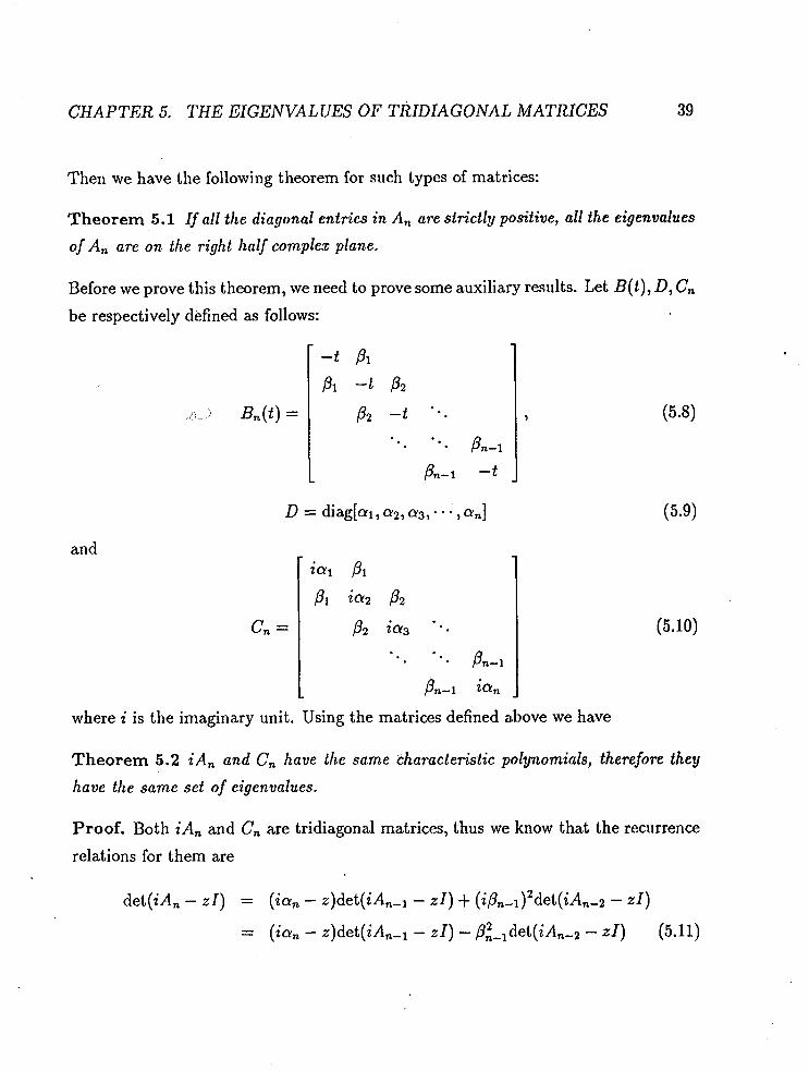
Then we have the following theorem for such types of matrices:

Theorem 5.1 If all the diagonal entries in An are strictly positive, all the eigenva

of An are on the right half complex plane.

Before we prove this theorem, we need to prove some auxiliary results. Let B(t) , D, C, be respectively defined as follows:

and

where i is the imaginary unit. Using the matrices defined above we have

Theorem 5.2 iAn and Cn have the same characteristic polynomials, therefore they

have the same set of eigenvalues.

Proof. Both iAn and Cn are tridiagonal matrices, thus we know that the recurrence

relations for them are

det(iAn - zI ) = (ian - ~)det( iA,-~ - zI ) + (iPnd1)2det(iAn-2 - zI)

CHAPTER 5. THE EIGENVALUES OF TRIDIAGONAL MATRICES 40

and

det(C, - r I ) = (in, - z)det(C,-I - zI) - &,det(~,_z - r I ) (5.12)

for n = 3,4,5, -. It can be easily verified that

det(iA, - 21) r det(Cn - 21) (5.13)

for n = 1,2. Therefore both characteristic polynomials are identical for any integer

number: n.

& 1 Theorem 5.3 C, has no real eigenvalue if all ni, i = 1,2, . . , n are strictly positive.

Proof. Assume that C, has a real eigenvalue t and let x + i y be the corresponding

eigenvector. Then we have

C,(X + iy) = t (x + iy),

or, (B(t) + iD)(x + iy) = 0.

(5.15) can be rewritten as

B(t)x- Dy = 0

and

or,

But

CHAPTER 5. THE EIGENVALUES O F TRIDIAGONAL MATRICES 41

thus

det [ '(') ] = *det (D)de t (~( t )D- '~( t ) + D). D '(t)

On the other hand,

and D- f B(~)D-; is a symmetric matrix so that B(t)D-'B(t)+D is a positive definite

matrix. Therefore, system (5.18) has only the trivial solution. This is contradictory

to the assumption at $he beginning. h

Theorem 5.4 A, has no pure imaginary eigenvalue under the same condition in

Theorem 5.1.

Proof. This is quite staightforward since iA, and C, have the same set of eigenvalues.

0

Now a proof of Theorem 5.1 could be given.

Proof of Theorem 5.1. Let

Then A(0) = D, A(l) = A, and all the eigenvalues of A(s), Aj, j = 1,2, , n, are

continuous functions of s since eigenvalues of a matrix are continuous functions of its

entries. When s = 0, obviously Xj(0) = aj, j = 1,2, . , n; thus all eigenvalues are

on the right half plane. For any 0 < s 5 1, the condition in Theorem 5.1 for A, is satisfied, thus A(s) has no pure imaginary eigenvalue. Therefore, no eigenvalue of

A(s) can go to the left half plane without crossing the imaginary axis. This implies

that all the eigenvalues of A(s) stay on the right half plane, i.e.,

CHAPTER 5. THE EIGENVALUES OF TRIDIAGONAL MATRICES

In particular,

Re{Xj) = Re{Xj(l)) > 0, j = 1,2, - , n

where Xj, j = 1,2, . , n are the eigenvalues of A,.

As a consequence of Theorem 5.1, we have:

Theo rem 5.5 If all diagonal entries in A, are strictly negative, then all eigenvalues

of A, are on the left half plane.

Furthermore we have the following result under a slightly different condition. a:

Theorem 5.6 If A, satisfies the conditions in Theorem 5.1 except that a1 = 0, the

statement in Theorem 5.1 is still true.

Proof. From the proof of Theorem 5.1 we know that the key point is to show that

the matrix in system (5.18) is nonsingular, or to show that the following matrix

is nonsingular for any real number t . Let

and

Then Dl is positive definite. There can be only two cases for t:

(i) t is not eigenvalue of B(0) then B(t) is invertible;

(ii) t is an eigenvalue of B(O), then t is not an eigenvalue of B1(0) and thus Bl(t) is

invertible.

CHAPTER 5. THE EIGENVALUES OF TRIDIAGONAL MATRICES 43

Case (i). We have

det [ '(') ] = & d e t ( B ( t ) ) d e t ( ~ ~ - ' ( t ) ~ + B). D B(t)

Similar to the proof of Theorem 5.1 it could be verified that above determinant is 6, j

nonzero.

Case (ii). For simplicity we will drop t in Bl(t) and denote both 0 and oT by 0

from now on. We can make following multiplication for T:

Let

and

CIIAPTER 5. THE EIGENVALUES OF TRIDIAGONAL MATRICES 44

Then it is not difficult to prove that E is positive def nite since Dl is positive definite

and B1 is symmetric. From this notation one sees that

Therefore,

= f det(Dldet(E)[b~~-'b,(b:E-'b~ - cl) - (t + b :~ -*b~)~ ]

since bFE-'bz = bTl3-l bl. Thus we only need to prove that

From (5.33) we know that


Table 5.1: The statement not true for k = 6.

1

where PI = ( D r t B1) E-I (D;T BI) - ' . Therefore all eigenvalues of PI are strictly

positive since E-I is positive and similar to PI, and P is positive definite.

Remark 5.1 An interesting question is, if a; = 0 , l 5 i 5 k < n, does the result still

hold? Some numerical examples indicate that k could be larger than one, but what is

the largest k ? This is attractive to me and maybe to some readers as well.

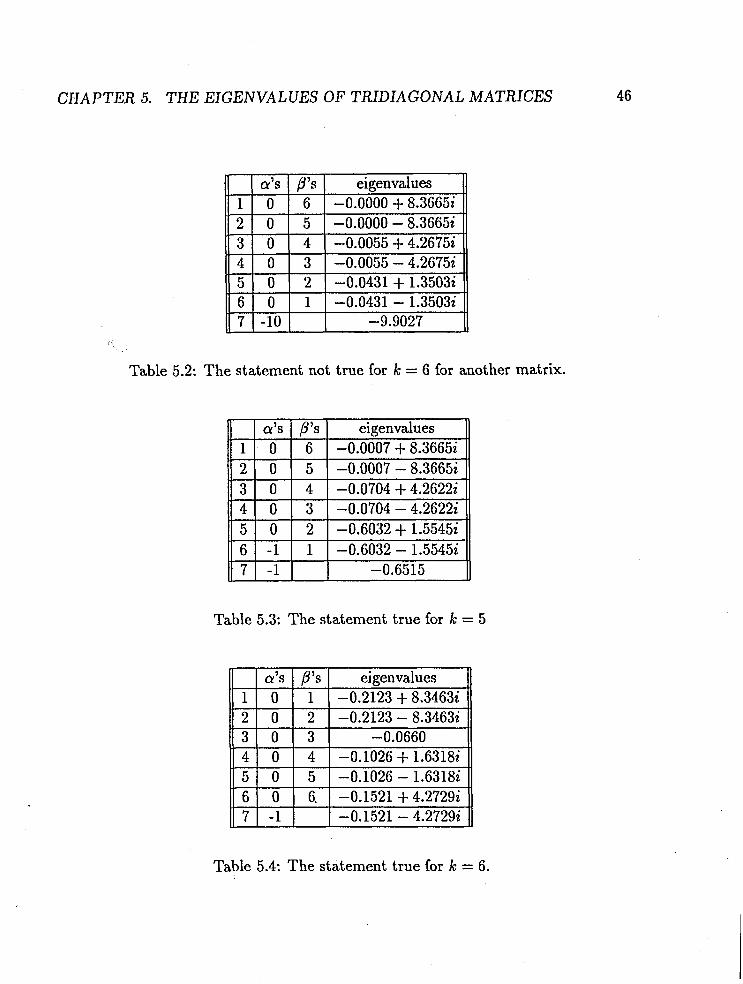
Examples. Table 5.1 to Table 5.4 give some examples of the eigenvalues of tridiag-

onal matrices. From Table 5.1 and Table 5.2, we see that the real part of the first

two eigenvalues should be zero. The next two tables show the cases that k = 5,6

respectively.


Table 5.2: The statement not true for k = 6 for another matrix.

-

Table 5.3: The statement true for k = 5

a's 0 1

I a's 1 I 0

a's P's eigenvalues ..

1 0 1 -0.2123 + 8.34632'

Table 5.4: The statement true for k = 6 .

P's 6

,8's 6

eigenvalues -0.0000 + 8.36652'

eigenvalues -0.0007 4- 8.36652'

Bibliography

I \ ,

[I] BARDOS,C. AND DEGOND,P., Global existence for the Vlasov-Poisson equa-

tion in 3 space variables with small initial data. Ann. Inst. Henri Poincare,

Analyse Nonlinear, 2, 101-118(1985).

[2] BATT,J., The present state of the existence theory of the Vlasov-Poisson and the

Vlasov-Maxwell system of partial differential equations in plasma physics. Proc.

Conf., Rome, 1984, Eds V . Boffi and H. Neunzert, Applications of mathematics

in technology, 375-385, Teubner, Stut tgart (1984).

[3] BENILAN, P., BREZIS,H. AND CRANDALL,M.G., A semilinear elliptic equa-

tion in L"RN). Ann. Sc. Norm. Sup. Pisa. 2, 523-555(1975).

141 BOYD,J.P., The rate of convergence of Hermite function series. Math. Comp.

35, 1039-1316(1980).

[5] BOYD,J.P., Chebyshev and Fourier Spectral Methods. (Springer-Verlag, Berlin,

[6] CANUTO,C., HUSSAINI,M.Y.,QUARTERONI,A. AND ZANG,T.A., Spectral

Methods in Fluid Mechanics. (Springer Verlag, Heidelberg, 1988).

[7] CARTLING,B., Kinetics of activated processes from nonstationary solutions of

the Fokker-Planck equation for a bistable potential. J. Chem. Phys. 87, 2638

-2648 (1987).

BIBLIOGRAPHY 48

[8] CHANDRASEKNAR,S., Stochastic ~roblems in physics and astronomy. Rev.

Mod. Phys. 15, 1-89(1943).

[9] CIARLET,P.G., The Finite Element method for Elliptic Problems. (North-

Holland Pub. Co., Amsterdam, 1978).

[lo] COURANT,R., Methods of Mathematical Physics. ( Interscience Publishers, Inc.,

New York, 1953).

[fl] DEGOND,P. AND MAS-GALLIC,S., Existence of solutions and diffusion ap-

proximation for a model Fokker-Planck equation. (Preprint, 1985).

[12] DIPERNA, R.J. AND LIONS, P.L., On the Fokker-Planck-Boltzmann equation,

Commun. Math. Phys., 120, 1-23 (1988).

[13] FUNAR0,D. AND KAVIAN,O., Approximation of some diffusion evolution

equations in unbounded domains by Hermite functions. Math. Comp. 57, 597-

619(1991).

[14] GOLDSTEIN,J.A., Semigroups of Linear Operators and Applications. (Claren-

don Press, Oxford, 1985).

[15j GOTTLIEB,D. AND ORSZAG,S., Numerical AnaIysis of Spectral Methods,

Theory and Applications. CBMS-NSF Regional Conference Series in Applied

Mathematics. 26. ( S I A M , Philadelphia, 1977).

[16] LEBEDEV,N.N., Special Functions and Their Applications. (Prentice-HaII, En-

glewood Cliffs, 1965 ).

[17] MOORE,P. AND FLAHERTY, J., Adaptive local overlapping grid methods for

parabolic systems in two space dimensions J. Comp. Phys. 98, 54-63(1992).

[18] PARLETT,B.N., The Symmetric Ez'genvalue Problem. (Prentice-Hall, Englewood

Cliffs, 1980 ).

BIBLIOGRAPHY 49

[19] PAZY,A., Semigroups of Linear Operators and Applications to Partial Difleren-

tial Equations. (Springer Verlag, New York, 1983).

[20] PERTHAME, B., Higher moments for kinetic equations: the Vlasov-Poisson and

Fokker-Planck cases, Math. Meth. App. Sci. 13, 441-452(1990).

[21] RIGHTMYER,R.D. AND MORTON, K.W., Diflerence Methods for Initial-Value

Problems,2nd ed. (Interscience Publishers, New York, 1965).

€221 RISKEN,H., The Fokker-Planck Equation: Methods of Solution and Applications. 4

J 2nd ed. (Springer Varlag,Berlin,l989).

[23] RINGHOFER, C., A spectral method for the numerical simulation of quantum

tunneling phenomena, SIAM J. Numer. Anal. 27,32 (1990).

[24] STRIKWERDA, J.C., Finite Digerenee Schemes and Partial Digerential Equa-

tions. (Wadsworth & Brooks /Cole, Belmont, 1989).

[25] TANG,T., The Hermite spectral method for Gaussian type functions. To appear

in SIAM J. Sci. Statist. Comput.

[26] TANG,T., MCKEE,S. AND REEKS,M.W., A spectral method for the numerical

solutions of a kinetic equation describing the dispersion of small particles in a

turbulent. J. Comput. Phys., ( To appear ).

[27] TROTTER,H.F. Approximation of semi-groups of operators, Pacific J. Math.,

8, 887-919(1958).

[28] WEIDEMAN,J.A.C., The eigenvalues of Hermite and rational spectral differen-

tiation matrices. Numer. Math., 61, 409-431(1992).

[29] WILKINSON,J.H., The Algebraic Eigenvalue Problem. ( Clarendon Press, Ox-

ford 1965).

[30] YOSIDA,K., Functional ~ n a l ~ s i s . 5th ed. (Springer Verlag, Heidelberg,l978).

a theoretical and numerical study for the fokker-planck...

Documents