a techno-economic analysis of decentralized electrolytic
TRANSCRIPT

A Techno-Economic Analysis of Decentralized Electrolytic Hydrogen Production for Fuel Cell Vehicles
Sibastien PrinceRichard B.A.Sc., Universiti Laval, 1996
A Thesis Submitted in Partial Fulfillment of the Requirements for the Degree of
MASTER OF APPLIED SCIENCE
in the Department of Mechanical Engineering
I
0 Skbastien Prince-Richard, 2004
University of Victoria
All rights reserved. This thesis may not be reproduced in whole or in part, by photocopy or other means, without the permission of the author

Supervisor: Dr. Nedjib Djilali
Hydrogen fi-om decentralized water electrolysis is one of the main fuelling options considered
for future fuel cell vehicles. In this thesis, a model is developed to determine the key technical
and economic parameters influencing the competitive position of decentralized electrolyhc
hydrogen. This model, which incorporates the capital and energy costs of water electrolysis,
as well as a monetary valuation of the associated greenhouse gas (GHG) emissions, is used to
analyze the competitive position of electrolytic hydrogen in three specific locations with
distinct electricity mix: Vancouver, Los Angeles and Paris. Using local electricity prices and
fuel taxes, electrolytic hydrogen is found to be commercially viable in Vancouver and Paris.
Hydrogen storage comes out as the most important technical issue. But more than any
techcal issue, electricity prices and fuel taxes emerge as the two dominant issues affecting
the competitive position of electrolytic hydrogen. The monetary valuation of GHG emissions,
based on a price of $20/ton of C02 , is found to be generally insufficient to tilt the balance in
favor of electrolytic hydrogen.

ABSTRACT ................................................................................................................................. I1
........................................................................................................... TABLE OF CONTENT I11
LIST OF TABLES ..................................................................................................................... VI LIST OF FIGURES ............................................................................................................... VIII
NOMENCLATURE ....................................................................................................................
ACKNOWLEDGEMENTS ................................................................................................. XI11
CHAPTER 1 . INTRODUCTION ..................................................................................... . . 1
1.1 RATIONALE ........................................................................................................................... 1
1.2 FUEL CELL VEHICLES ........................................................................................................... 3
1.3 GREENHOUSE GASES AND CLIMATE CHANGE .................................................................... 6
1.4 HYDROGEN PRODUCTION TECHNOLOGIES ......................................................................... 9
1.5 FACTORS ~~FLUENCING THE DEVELOPMENT OF A REFUELLING NFRASTRUC?ZTRE ......... 11
............................................................................................................... 1.5.1 Fuel Options 11
.......................................................................................... 1 S.2 Trends in Energy Markets 12
................................................................................................................ 1 S.3 Externalities I 3
1.5.4 Energy Security ........................................................................................................... 13
..................................................................... 1.6 FOCUS AND METHODOLOGY OF THIS STUDY 13
....................................................................................................................... 1.7 PRIOR WORK 17
................................................................................................ 1.7.1 Fuel choices for FCVs 17
.............................................................................................. 1.7.2 The Electrolysis Option 18
............................................................ 1.7.3 The Influence of Greenhouse Gas Emissions 19
.......................................... CHAPTER 2 - WATER ELECTROLYSIS BACKGROUND 20
.......................................................................................................................... 2.1 PRINCIPLES 20
2.1.1 Alkaline Water Electrolysis ( A m ) ........................................................................... 21
.............................................................................. 2.1.2 Solid Polymer Electrolysis (SPE) 23
..................................................................... 2.1.3 High Temperature Electrolysis (HTE) 2 6
............................................................................ 2.1.4 Basic Electrolyzer Configurations 2 7
2.2 ENERGY USE ....................................................................................................................... 29
2.2.1 Thermodynamics ........................................................................................................ 29 . .
2.2.2 E@czenczes .................................................................................................................. 34
2.2.3 Cell Voltage ................................................................................................................ 35
2.2.4 Efect of Operating Conditions .................................................................................. 38
2.2.4.1 Temperature ....................................................................................................... 3 8
2.2.4.2 Pressure ................................................................................................................ 38
2.2.4.3 Current density .................................................................................................... 40
2.2.5 Overall Energy Use of an Electrolyzer Cell ............................................................. 4 2
2.3 TRENDS IN WATER ELECTROLYSIS TECHNOLOGIES .......................................................... 43
2.3.1 Decrease Energy Use ................................................................................................. 44
................................................................................................. 2.3.2 Reduce Capital Cost 4 6
2.3.3 Synergy with Fuel Cell Developments ....................................................................... 47
2.4 SUMMARY OF ELECTROLYSIS TECHNOLOGIES AND MAIN PLAYERS ................................ 47
CHAPTER 3 - COST MODEL ........................................................................................... 5 1
........................................................................................... 3.1 GENERAL CONSIDERATIONS 5 1
3.2 DESCRIPTION OF THE MODEL ............................................................................................. 52
................................................................................ 3.2.1 C, . Capital and Operating Cost 54
.......................................................................................................... . 3.2.2 C, Energy Cost 62
......................... 3.2.3 Cm: Relative Cost or Saving Due to GHG Emission Evaluation 69
3.3 SITE-SPECIFIC INFORMATION ........................................................................................... 7 4
3.4 COST COMPARISON WITH OTHER FUELLING OPTIONS ...................................................... 76
3.5 VALIDATION OF THE COST MODEL ................................................................................... 7 7
CHAPTER 4 - ANALYSIS ...................................................................................................... 80
4.1 APPROACH ........................................................................................................................... 80
............................................................................ 4.2 BASE CASE FOR SENS~TIV~TY ANALYSIS 82
4.3 SENSITIVITY ANALYSIS FOLLOWING THE COST MODEL STRUCTURE ............................... 84
.............................................................................................. 4.3.1 Capital and O M Cost 84
4.3.2 Energy Cost ................................................................................................................. 87
....................................................................................... 4.3.3 GHG Added Cost or Saving 89
4.4 ANALYSIS FROM THREE PERSPECTIVES ............................................................................. 93
4.4.1 InjluencesJi.om a Technical Perspective ................................................................... 98
4.4.1 . 1 Hydrogen Storage .............................................................................................. 9 8
4.4.1.2 Electrol yzer ........................................................................................................ 101
4.4.1.3 Compression ...................................................................................................... 103
4.4.1.4 Use of Natural Gas ............................................................................................ 103
.............................................................. 4.4.2 Influences Ji.om an Economic Perspective 104
............................................................... 4.4.2.1 Electricity Price and Capacity Factor 104
................................................. 4.4.2.2 Financing Scheme and Economic Parameters 107
.................................................................................... 4.4.2.3 Other Economic Issues 1 1 0
........................................................... 4.4.3 InJuencesfiom a Comparative Perspective 112
......................................................... 4.4.3.1 C02 Emissions and Monetary Valuation 113
...... 4.4.3.2 Comparison of Electrolytic Hydrogen and Gasoline in Three Locations 115
........................................................................... 4.4.3.2.1 Electricity Price and Mix 117
4.4.3.2.2 Taxes and Credits on Fuels ....................................................................... 118
4.4.3.2.3 Fuel Economy Improvements ................................................................... 120
.................................................................. 4.5 OVERALL SUMMARY OF ANALYSIS RESULTS 121
CHAPTER 5 - CONCLUSIONS AND F'UTURE PERSPECTIVES ............................. 125
.............................................................................................. 5.1 THE APPROACH REVISITED 125
....................................................................... 5.2 CONCLUSIONS AND RECOMMENDATIONS 126
5.3 FUTURE WORK ................................................................................................................. 131
REFERENCES ......................................................................................................................... 133
.... APPENDIX A . THERMODYNAMIC VOLTAGES FOR WATER SPLITTING 139
APPENDIX B . FUEL ECONOMY CONVERSIONS ..................................................... 146
APPENDIX C . COST MODEL DEVELOPED IN MICROSOFT EXCEL ............... 149
APPENDIX D . BASE CASE VALUES FOR SENSITIVITY ANALYSIS .................. 171
APPENDIX E . SITE-SPECIFIC INFORMATION ....................................... 1 8 0

List of Tables
Table 2.1 : Example of ohmic resistances and cell voltage elements ......................................... 37
Table 2.2: Theoretical energy use of water electrolysis as a function of pressure and
temperature. based on reversible voltage LV. thermoneutral voltage &. and higher-
heating-value voltage EHHV (assuming current efficiency of 100%) ................................ 43
Table 2.3 : Typical operating conditions and energy use of commercial electrol yzers ............. 43
Table 2.4. Present and advanced electrolyser technologies at a glance ..................................... 50
Table 3.1 : Example of electricity mix and specific GHG values used in the model ................ 73
Table 3.2. Site-specific information input ................................................................................... 75
Table 4.1 : Electrolyzer station relative sizes ............................................................................... 85
Table 4.2: Parameters used to calculate the annual capital and O&M cost (C, ) of a
decentralized electrolytic hydrogen dispensing station ...................................................... 86
Table 4.3: Parameters used to calculate the annual energy cost (Ce) of a decentralized
electrolyhc hydrogen dispensing station ............................................................................. 88
Table 4.4: Parameters used to calculate the annual "GHG added cost or saving" (CGHG)
associated with a decentralized electrolytic hydrogen dispensing station ........................ 90
Table 4.5. List of "issues" associated with the parameters used in the cost model ................... 96
Table 4.6: Values used to estimate the maximum cost reduction achievable through technical
improvements ..................................................................................................................... 105
......................... Table 4.7. Parameters affecting the effective capital recovery factor (CRFe) 108
Table 4.8: Assumptions and values used for the cost comparison of electrolybc hydrogen with . . . .
gasoline m three cities ........................................................................................................ 115
Table A.l: Values used to calculate the higher-heating-value voltage (Em) as a function of
......................................................................................................................... temperature 143
...... Table A.2. Summary table of the relevant voltages used for the water-splitting reaction 145
Table D . 1 : Base case values and range for parameters used to determine the hydrogen demand
......................................................................................................... of the fuelling station 172
Table D.2: Base case values and range for parameters used to calculate the "Capital and
O&M" costs of the fuelling station ................................................................................... 175

Table D.3: Base case values and range for parameters used to calculate the "Energy" costs of
............................................................................................................ the fbelling station.. 177
Table D.4: Base case values and range for parameters used to calculate the "GHG Added Cost
or Saving" of the fuelling station ..................................................................................... 179
Table E. 1 : Site-specific information to compare the price of electrolytic hydrogen and gasoline
List of Figures
Figure 1.1 : 80 kW light-duty fuel cell engine developed by Ballad Power Systems ................ 4
Figure 1.2: Examples of fuel cell vehicles . Hy-wire fuel cell car developed by General Motors
and fuel cell bus model produced by DaimlerChrysler for the CUTE project in Europe . 5
Figure 1.3: IPCC estimates of C02 atmospheric concentration to 2100 for their six marker
scenarios (IS92) ..................................................................................................................... 7
Figure 1.4. Optimistic growth rate of hydrogen cars in world market ...................................... 12
Figure 1.5. Path analyzed in reference to the architecture of energy systems ........................... 14
Figure 1.6. Aspects of decentralized water electrolysis investigated ......................................... 15
Figure 2.1 : Principle of alkaline water electrolysis (AWE) ....................................................... 20
Figure 2.2. Principle of solid polymer electrolysis (SPE) .......................................................... 23
................................................. Figure 2.3. Example structure of a sulphonated fluoropolymer 24
.................................................. Figure 2.4. Principles of high temperature electrolysis (HTE) 26
.......................................................... Figure 2.5. Principles of a tank electrolyzer (monopolar) 27
Figure 2.6. Principles of a filter-press electrolyzer (bipolar) ...................................................... 27
Figure 2.7. (a) Series connection and (b) "Parallel and series" connection of electrolyzers .... 28
Figure 2.8. Simplified process diagram for hydrogen production by water electrolysis .......... 29
Figure 2.9. Theoretical water electrolysis voltages as a function of temperature ..................... 33
Figure 2.10. Voltage vs . current density relationships ............................................................... 36
Figure 2.1 1 : Ideal electrolyzer/compressor energy use per kilogram of hydrogen . Electrolyzer
efficiency = 100% at 80 OC, compressor efficiency = 75% single-stage adiabatic
compression ......................................................................................................................... 40
Figure 2.12. Relative electrode surface area as a function of current density ........................... 41
Figure 2.13: Current-voltage plots of conventional HTE and NGASE . Cathode inlet gas: H2
............... (3%) + H20 (70%) + N2 (balance) . Anode inlet gas: CH4 (97%) + H20 (3%) 45
Figure 3.1 : General structure of the cost model .......................................................................... 54
.......................... Figure 3.2. Components included in the electrolyzer station capital cost C, 58
............................................ Figure 3.3. Components of the annual multiplying factor for C,, 60
.............. Figure 3.4. Simplified process diagram for electrolytic hydrogen dispensing station 62
Figure 3.5. Annual cost of energy for the electrolyzer station ................................................... 64
Figure 3.6. Theoretical electrolysis voltages as a bc t ion of temperature ............................... 65
Figure 3.7. Annual cost of energy for the compressor subsystem ........................................ 67
Figure 3.8: Example of output from the cost model. showing how the relative GHG
costhaving component can be ignored or included for comparison with each of the
alternative helling options .................................................................................................. 70
Figure 3.9. Annual cost or saving associated with GHG emissions ......................................... 71
Figure 3.10. Fuel cost comparison on a per-kilometer basis in the model ................................ 76
................ Figure 3.1 1 : Validation of the model's financing aspect reproducing DTI's results 77
Figure 3.12: The model's ability to reproduce DTI's results for various sizes of electrolyzer
................................................................................................................................. stations 7 8
....... Figure 3.13 : The model's ability to reproduce DTI's specific hydrogen cost distribution 78
Figure 4.1. Aspects considered in sensitivity analysis ................................................................ 80
............................................................ Figure 4.2. Dependence on geo-economic environment 81
.................................................................. Figure 4.3. Dependence on other helling options 8 2
............................... Figure 4.4. Distribution of the delivered hydrogen price for the base case 84
Figure 4.5: Sensitivity of hydrogen price to parameters affecting the Capital and O&M cost
....................................................................................................................................... (CJ 8 7
Figure 4.6. Sensitivity of hydrogen price to parameters affecting the Energy cost (C, ) ........... 89
Figure 4.7: Sensitivity of hydrogen price to parameters affecting the GHG costhaving
component (CGHG) ............................................................................................................... 92
Figure 4.8. Perspectives considered in the second part of the analysis ................................ 94
Figure 4.9: Mapping of parameters in terms of hydrogen price sensitivity and aspects
influenced ............................................................................................................................ 9 5
Figure 4.10: Distribution of issues affecting the price of hydrogen from decentralized
electrolysis ............................................................................................................................ 97
Figure 4.1 1 : Impact of hydrogen storage requirements for personal appliance case (2 FCVs. D
= 11.4) and larger station (base case: 100 FCVs. D = 2) ................................................... 99
Figure 4.12: Relative impact of electricity price vs . ideal techcal improvements (Ideal
.......................................................................... technical performance) for the base case 104

Figure 4.13: Sensitivity of the effective capital recovery factor (CRF,) to various economic
parameters under three different financing scenarios (B: business, U: utility, H: home
mortgage) ........................................................................................................................... 108
Figure 4.14: Impact of financing scenario on hydrogen price for two different sizes of
electrolyzer stations. The unit capital cost of electrolyzer, compressor and storage
components are the same for the two sizes. O&M represents the same % of capital cost
for each electrolyzer station's size. ............................................................................... 1 10
Figure 4.1 5: Impact of the volume of electrolyzer stations manufactured on the hydrogen cost
fiom a previous study by Thomas et al ............................................................................. 1 1 1
Figure 4.16: Life-cycle COz emissions per kilometer fiom a FCV using electrolyhc hydrogen
as a function of electricity mix (solid line), compared to C02 emissions of other fbel
options. ............................................................................................................................... 1 13
Figure 4.17: Site-specific comparison of gasoline and electrolytic hydrogen retail price . .
including taxes and the effect of credits for low C02 ermssions. .................................... 1 16
Figure 4.18: Breakeven condition (solid line) for untaxed electrolytic hydrogen to compete
with taxed gasoline. Electricity prices to the left of the solid line would result in
....... electrolytic hydrogen being less expensive than gasoline on a per-lulometer basis 11 8
Figure 4.19: Breakeven condition for taxed electrolytic hydrogen to compete with taxed
gasoline.. ............................................................................................................................. 1 19
Figure 4.20: Breakeven condition for taxed electrolytic hydrogen to compete with taxed
gasoline used in an ICE vehxle with improved fuel economy (50% longer driving range
................................................................................................... on same amount of hel). 1 2 1
Figure 4.21: Final distribution of issues affecting the price of hydrogen fiom decentralized
........................................................................................................................ electrolysis.. 122
Figure 4.22: Overall summary of the impact of issues affecting the competitive position of
......... electrolytic hydrogen &om a techcal, economic and comparative perspective. .I24
............................ Figure 5.1 : Schematic of the three perspectives considered in the analysis 126
Figure A. 1 : Theoretical water electrolysis voltages as a function of temperature (at 1 bar). .I39
Figure A.2: Schematic of the simplified electrolysis process used to calculate the theoretical
energy requirement of the process. ................................................................................... 140

Nomenclature
ACJDC: alternative currentldirect current
AWE: alkaline water electrolysis
CaFCP: California Fuel Cell Partnership
CB&H: Carbon Black and Hydrogen
CDM: clean development mechanism
C&: methane
CO: carbon monoxide
COT: carbon dioxide
CRF: capital recovery factor
CRF,: effective capital recovery factor
CTFCA: Canadian Transportation Fuel Cell Alliance
CUTE: Clean Urban Transportation for Europe
DOE: United States Department of Energy
DTI: Directed Technologies Inc.
EPA: U.S. Environmental Protection Agency
FCV: fbel cell vehicle
GHG: greenhouse gas
H2: hydrogen
H20: water
HHV: higher heating value
HTE: htgh temperature electrolysis
HVRA: hydrogen vehicle refbelling appliance
ICE: internal combustion engine
IET: international emission trading
ME: inorganic membrane electrolysis
IPCC: Intergovernmental Panel on Climate Change
KOH: potassium hydroxide
kW,: kilowatt electric
LHV: lower heating value

LLNL: Lawrence Livermore National Laboratory
MEA: membrane electrode assembly
MeOH: methanol
mpgge: mile per US gallon gasoline equivalent
NEDO: New Energy and Industrial Technology Development Organization
NG: natural gas
NGASE: natural gas assisted steam electrolysis
NO,: nitrous oxides
NREL: National Renewable Energy Laboratory
O&M: operation and maintenance
PEM: proton exchange membrane
PEMFC: proton exchange membrane fuel cell
POX: partial oxidation
PTFE: polytetrafluoroethylene
R&D: research and development
RFC: regenerative fuel cell
SMR: steam methane reforming
SOFC: solid oxide fuel cell
SPE: solid polymer electrolysis
STP: standard temperature and pressure
UNFCCC: United Nations Framework Convention on Climate Change
URFC: unitized regenerative he1 cell
WE-NET: World Energy Network
ZEC: Zero Emission Coal
ZEV: zero emission vehicle

Acknowledgements
The completion of th~s thesis marks a very important step in life for me. Of course, a thesis
generally represents an academic achievement in itself, but to me the real learning experience
has been on the personal level. Most graduate students who have attempted to write a thesis
while worlung full-time understand how it can mysteriously transform itself o v a time fiom a
stimulating research into a monster out of proportions. Well, in my case, it has taken longer
than I would ever have imagined to finish it. But I finally get the impression that the monster
has been tamed and that I can go on with my normal life. It has been quite a journey, and I
have many people to thank for their understanding and support during these years.
First, I owe a big thanks to my thesis supervisor, Ned Djilali, who has always been extremely
considerate. He quickly understood the kind of person I was, and provided all the autonomy,
flexibility a d encouragements that I needed, in addition to the type of advice that can
normally be expected fiom a thesis supervisor.
Then, there is my family. I want to thank deeply Louise, Francpis and Sarah for their
indefectible support. They were kind enough to put up with my moods at all times,
particularly during the last year. My mother Louise deserves a special mention for her
devoted assistance during crucial periods. I also want to express my gratitude to close hends:
Britta Bossel, Frankie-Lou Fuller, Walter Merida and FrWric Dugre, who have been sources
of inspiration and an important support throughout tough times.
Last but not least, I must thank Bruce Pridmore, Chris Ryan, Aileen McManamon, Walter
Pickering and many former colleagues who have been very understanding and
accommodating during my time with the National Research Council.
Finally, I keep a rich impression of the many people I have had the chance to know more
personally at the Institute for Integrated Energy Systems (IESVic). Ned Djilali, David Scott,
MacMurray Whale and Ged McLean in particular have contributed, by their teachmg and their
enthusiasm, to shape my vision of future energy systems for a better world. All these people
have fed my ambitions to become an active player in the profound transformations towards a
sustainable world, where technology and the environment can coexist in harmony.

Chapter 1 - Introduction
1.1 Rationale
Severe degradation of urban air quality in a growing number of cities around the globe has
prompted the adoption of stricter legislation to reduce polluting emissions, particularly from
transportation. The State of California has been a leader in this respect, with the introduction
of its 1989 legislation requiring that 2% of total vehicle sales in 1998 and 10% in 2003 be zero
emission vehicles (ZEV) [I]. Although these targets have been revised a few times since, the
legislation triggered more intense efforts in the development of cleaner energy technologies
such as fuel cells, advanced batteries and hybrid vehicles, to significantly reduce polluting
emissions from transportation.
As a result, fuel cells and hydrogen have been at the forefront of technology developments for
a few years now, not only in transportation but across the whole energy sector. The
technology has attracted sizeable investments and achieved significant technical progress. It is
receiving growing support from governments and the private sector, in leading countries lrke
the United States, Canada, Japan or Germany [2], but also in less technologically advanced
countries facing serious environmental problems, like China [3]. Today, a wide spectrum of
industries are involved concretely in fuel cell activities: carmakers, oil companies, power
utilities, portable electronics, etc.
Immediate concerns about the effects of toxic air pollutants may have been a trigger for the
development ,of cleaner energy technologies like fuel cells, but another type of pollution linked
to transportation may have much more profound repercussions in the long term: the so-called
greenhouse gas (GHG) emissions. Attributable primarily to the combustion of fossil fuels,
GHG emissions from anthropological sources have become a serious threat to ecosystems and
W e generations because their effects are felt globally and on a much longer time scale.
Global warming caused by increasing levels of GHG in the atmosphere could lead to climate
disruption and a multitude of adverse consequences, often irreversible. The issue gained
credibility d&ng the 1990s and resulted in the much publicized Kyoto Protocol in 1997.
Aimed at reducing GHG emissions internationally, the Protocol constitutes a first step in the

right direction, but curbing GHG emissions to sustainable levels will require hdamental
changes in energy systems.
Fuel cell vehicles (FCV) have the potential to completely eliminate harmful tailpipe emissions
without compromising vehicle performance or range. However, their ability to cut back GHG
emissions globally depends largely on the choice of fuel and its distribution infiastructure.
Hydrogen is the fuel required for the fuel cells per se, but it can be obtained from a variety of
sources or extracted onboard fiom a hydrocarbon fuel. The choice of fuel ought to maximize
the long term benefits of replacing internal combustion engine (ICE) vehicles by FCVs,
particularly with respect to GHG emissions. On the other hand, a successful strategy for
introducing FCVs must minimize the technical and economic barriers that could prohibit or
significantly delay the adoption of FCVs. That is why fuelling is such a central issue in the
development of fuel cell systems in transportation.
Hydrogen, methanol and gasoline are currently the three most seriously considered fuel
options. Primarily because of economic considerations, they would all be largely produced
fiom fossil fuel sources in the near future. One problem in using fossil fuels as a feedstock is
their associated emissions, in particular GHG. Hydrogen generated fiom fossil fuels, either
onboard vehicles or at a stationary plant, invariably releases carbon-containing byproducts,
generally in the form of C02. Even hydrogen produced fiom stationary steam reforming of
natural gas, considered as the economically feasible option with the most significant
reductions in GHG emissions, still emits 30-60% of the GHG emissions from a gasoline ICE
vehcle, when used in a FCV [4-51.
Hydrogen from water electrolysis constitutes an inherently more flexible option with respect
to the energy input required and the associated GHG emissions. Electrolysis can make use of
the electrical and water infiastructure already available in many areas. It also provides access
to nuclear and renewable energy sources, which have very low GHG emissions. Moreover, an
interesting synergy between similar aspects of water electrolysis and fuel cell technologies
could have a noticeable impact on the development and cost of the electrolytic hydrogen
fuelling option. Electrolyzers can be scaled-down relatively easily compared to other options,
which may be an important advantage for the smooth market penetration of FCVs.

Accordingly, some electrolyzer companies have adopted a product development strategy that
emphasizes the decentralized production of electrolytic hydrogen for the future FCV market
[6-71.
The fbndamental goal of the present thesis is to identify key technical and economic
parameters that offer opportunities to maximize the competitive position of decentralized
electrolyhc hydrogen for FCVs. To do so, a model was developed that incorporates not only
the various capital and energy costs, but also a monetary valuation of the associated GHG
emissions. A sensitivity analysis was then performed to quantify the impact of various issues
fi-om three increasingly broader perspectives, namely: technical, economic and "comparative".
In the end, this integrated analysis provides a tool for directing more effectively the actions
required to improve the competitive position of electrolytic hydrogen for FCVs.
1.2 Fuel Cell Vehicles
Three broad approaches are being discussed these days when speaking of cleaner light-duty
vehcles: hybrids, battery electric, and fuel cell vehicles (FCV).
Hybrids generally refer to a combination of internal combustion engine (ICE) and batteries to
improve the overall energy efficiency of the vehcle. However, all of the energy in a hybrid
car still comes exclusively fi-om the combusted fuel, part of which is used to recharge the
batteries. The relative market success of introductory hybrid cars like the Toyota Prius and
Honda Insight have prompted most carmakers to announce the commercialization of several
more hybrid models in the coming years. Even though the hybrid approach can reduce
polluting emissions sensibly, mostly due to an increase in vehicle mileage of 20-40%, it
remains a partial and temporary solution for the long term.
Battery electric vehcles rely entirely on a bank of batteries to store electricity and use it to
power the vehicle. In this case, the actual source of energy depends on the electricity mix of
the recharging station. The main practical problems associated with battery electric vehicles
are a long recharging time and a limited range due to the much lower energy density of
batteries compared to hydrocarbon fuels.

FCVs are also electrically powered like battery electric vehicles. The difference lies in that the
electricity is produced onboard by fuel cells. A fuel cell is an electrochemical energy
conversion device that converts the chemical energy of a fuel into electricity and heat, without
combustion. When the fuel is pure hydrogen and the oxidant is oxygen fiom the air, there are
no tailpipe emissions other than water. A FCV can therefore combine the advantages of a
battery electric vehicle in terms of tailpipe emissions, and those of an ICE vehicle in terms of
energy density and ease of refbelling. Figure 1.1 shows an example of a hydrogen he1 cell
system for light-duty vehicles [8].
- Power L Distribution
Fuel Cell Stack Module ---------1
Control Unit
System Module
Unit
Jooling Pump
Figure 1.1: 80 kW light-duty fuel cell engine developed by Ballard Power Systems [8].
The type of fuel cell favored by all major carmakers is the proton exchange membrane fuel
cell (PEMFC). Because they are quite sensitive to contaminants, particularly carbon
monoxide, PEMFCs require relatively pure hydrogen as a &el. They cannot use other
hydrocarbon fbels directly either. Therefore, it leaves two possible fbel strategies: either
onboard hydrogen storage or onboard processing of a liquid fbel like gasoline or methanol to
extract hydrogen. Note that the latter option adds further complexity to the system and results
in some C02 and other trace emissions fiom the vehicle, along with water.
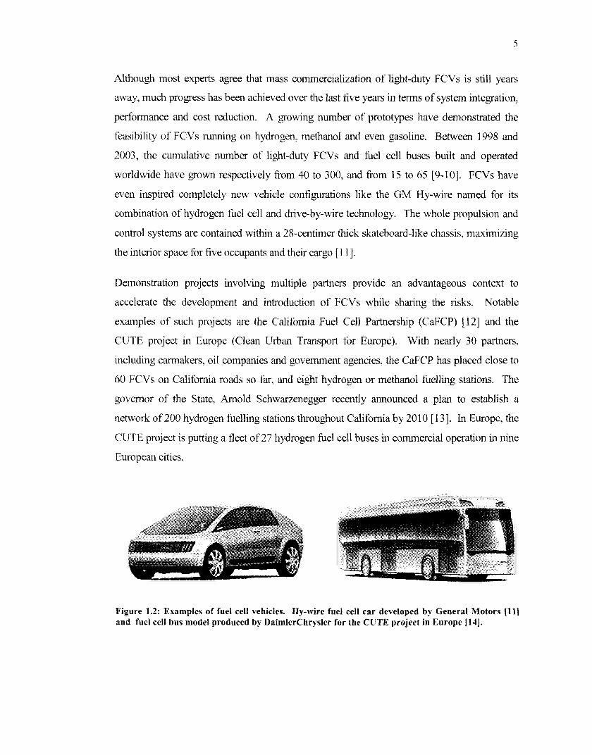
Although most experts agree that mass commercialization of light-duty FCVs is still years
away, much progress has been achieved over the last five years in terms of system integration,
performance and cost reduction. A growing number of prototypes have demonstrated the
feasibility of FCVs running on hydrogen, methanol and even gasoline. Between 1998 and
2003, the cumulative number of light-duty FCVs and &el cell buses built and operated
worldwide have grown respectively from 40 to 300, and fiom 15 to 65 [9-101. FCVs have
even inspired completely new vehicle configurations like the GM Hy-wire named for its
combination of hydrogen fuel cell and drive-by-wire technology. The whole propulsion and
control systems are contained within a 28-centimer thick skateboard-like chassis, maximizing
the interior space for five occupants and their cargo [ l I].
Demonstration projects involving multiple partners provide an advantageous context to
accelerate the development and introduction of FCVs whde sharing the risks. Notable
examples of such projects are the California Fuel Cell Partnerslup (CaFCP) [12] and the
CUTE project in Europe (Clean Urban Transport for Europe). With nearly 30 partners,
including carmakers, oil companies and government agencies, the CaFCP has placed close to
60 FCVs on California roads so far, and eight hydrogen or methanol fuelling stations. The
governor of the State, Arnold Schwanenegger recently announced a plan to establish a
network of 200 hydrogen fuelling stations throughout California by 2010 [ I 31. In Europe, the
CUTE project is putting a fleet of 27 hydrogen fuel cell buses in commercial operation in nine
European cities.
Figure 1.2: Examples of fuel cell vehicles. Hy-wire fuel cell car developed by General Motors [IS] and fuel cell bus model produced by DaimlerChrysler for the CUTE project in Europe 114).

1.3 Greenhouse Gases and Climate Change
The Earth's atmosphere is comprised of naturally occurring greenhouse gases (GHGs), such as
water vapor (H20), carbon dioxide (C02), nitrous oxides (NO,) and methane (CH4). These
gases form an insulating envelope around the planet that traps a portion of the heat received
from the Sun, which would otherwise be reflected back into space. Without this essential
envelope of GHGs, the Earth's mean temperature would be approximately 30•‹C lower, and the
planet would be unable to sustain life [15].
Based on scientific evidence, a strong correlation exists between atmospheric C02 level (by
far the dominant GHG) and temperature [16]. For thousands of years, a natural equilibrium
between sources and sinks of C02 has kept the pre-industrial atmospheric concentration of
C02 at about 280 ppmv (parts per million volume). Analyses of air trapped in the major
icecaps show that the range of C02 concentration has stayed between 180 and 280 ppmv over
the period of record of the last 400,000 years. Since the beginning of the Industrial Revolution
however, the concentration of C02 in the atmosphere has risen about 33% to 371 ppmv (in
2001), most of that rise occurring in the last 40 years. As a result of growing GHG emissions
from anthropogenic sources, largely due to the burning of fossil fuels, the current atmospheric
concentration and rate of increase of C02 are completely without precedent for at least the last
400,000 years [17].
Since the mean lifetime of C02 in the atmosphere is in the order of 100-1 50 years, the effects
of today's emissions will be felt well into the next century. The Intergovernmental Panel on
Climate Change (IPCC) has developed six emissions scenarios (IS92) to cover the range of
possible C02 emissions patterns until 2100. They reflect various combinations of population
and economic growth rates as well as certain fossil he1 constraints. One striking observation
is that even the most optimistic scenario predicts that C02 concentration should reach 500
ppmv sometime around the middle of th~s century, regardless of the rate of emissions
reduction. (Figure 1.3) [I 71.

Figure 1.3: IPCC estimates of C02 atmospheric concentration to 2100 for their six marker scenarios (IS92). [17]
Our only chance to stabilize C02 atmospheric concentration at double pre-industrial levels is
to ensure that by mid-century, the technologies and policies required to mitigate climate
change are widespread. In the energy sector, it means that nearly all new power generation
and transportation by then should have extremely low or zero GHG emissions. That is true
not only for industrialized countries that should lead the way, but also for developing countries
where most of the growth in energy use will take place, keeping in mind that developing
countries are expected to increase their GHG emissions to levels much closer to industrialized
countries. For example, C02 emissions in 1995 were of nearly 20 tons per capita in the USA
vs. 3 tons per capita in Chma [I 51.
The imperative for actions to reduce GHG emissions lies in the magnitude and irreversibility
of long term consequences related to global warming. The effects of global warming occur on
a global scale rather than locally or regionally as in the case of particulate emissions or acid
rain. Small variations in global temperature could lead to broader climate change patterns,
raise sea levels, alter forest and crops yields, and reduce potable water supplies [ I 81. Entire
ecosystems could be altered irreversibly, and densely populated coastal areas could be flooded
periodically or permanently. Some adaptation to the consequences of climate changes is
possible, but much is unpredictable, so common sense dictates a cautious approach.

Transportation is responsible for approximately 26% of GHG emissions in Canada [19], a
share that is representative of most industrialized countries. Therefore, any long term plan to
curtail GHG emissions must include actions in the transportation sector.
Recognizing the threat posed by rising concentrations of GHGs in the atmosphere, 150 nations
fiom around the world signed the United Nations Framework Convention on Climate Change
(UNFCCC) in 1992, to cut GHG emissions on a voluntary basis to 1990 levels by 2000. In
1997, the parties to the UNFCCC met in Kyoto and negotiated a protocol that established
legally binding limits or reductions in GHGs for industrialized countries.
The Kyoto Protocol also proposed flexible mechanisms to help countries achieve their
emission reduction targets. International Emission Trading (IET) allows industrialized
countries to trade emission reduction credits among themselves, while the Clean Development
Mechanism (CDM) enables them to finance emission reduction projects in other industrialized
or developing countries. But even if the Kyoto Protocol is adopted and l l l y implemented, it
merely represents the beginning of a solution to the GHG problem, as it would slow down
global warming only slightly, approximately 4-7% or 0.1 OC to 0.2 OC by 2 1 00 [ 1 51.
An embryonic market for trading C02 emission reductions has already started and it is
anticipated to become one of the largest commodity markets in the world. A fair amount of
economic modeling has been completed by government entities, industry-sponsored
consulting groups, academic institutions and national laboratories, predicting values for GHG
reductions in the range US$25.00 to $150.00 per ton of C02 equivalent. Most of the
transactions that have occurred so far are more in the US$3.00 - $20.00 range, prices
significantly lower than the projected ones, primarily due to a discount for regulatory risks
[20]. The projected and actual monetary values assigned to C02 emission reductions clearly
constitute an additional tool for informed policy.

1.4 Hydrogen Production Technologies
Hydrogen may be produced from a variety of feedstocks, using several technologies. They
can be divided in four broad categories: hydrocarbon based technologies (fossil fuels and
biomass), water electrolysis, biological production and therrnochernical cycles. Some are well
established technologies while others are still at the development stage.
In practice, only fossil fbels processing and water electrolysis are commercial methods for
producing hydrogen. For large scale production, the economics generally favor hydrogen
from fossil fbels. Since the bulk of industrial hydrogen produced today is used in large
chemical plants for petroleum refining, ammonia and methanol synthesis, fossil fbels are by
far the dominant feedstock. Water electrolysis is more suitable for industry sectors that
require very high purity hydrogen, like metallurgy, electronics and pharmaceuticals. Of the 45
million tomes or so of hydrogen produced worldwide annually, approximately 96% comes
from fossil fuel processing (48% natural gas, 30% oil, 18% coal) and only 4% from water
electrolysis [21]. An interesting observation is that the current world production of hydrogen
corresponds to the fuel requirements of some 200 million light-duty FCVs, or about one third
of the global number of light-duty vehcles on the road today.
The main processes employed in industrial hydrogen production are steam reforming, (SMR - steam methane reforming), partial oxidation (POX) and combinations of the two. In these
processes, the hydrocarbon fuel reacts with either water or oxygen to form carbon monoxide
(CO) and hydrogen (H2). In both cases, the resulting CO is further reacted with water to
produce additional H2 and C02 (water shift reaction). Notice that for SMR and POX, a
significant portion of the actual hydrogen produced comes from water, generally over 50%.
Pyrolyhc cracking is another interesting approach for hydrocarbons as it directly splits the
feedstock into hydrogen and a pure carbon product (carbon black). It is characterized however
by a low feedstock utilization and high emissions [2 11.
Although it now occupies a modest share of the hydrogen production market, water
electrolysis is in fact the oldest hydrogen production technology. Electrolyhc water splitting
was first demonstrated by Nicholson and Carlisle in 1800, in the early days of the industrial
revolution. Yet, it took about a century before it was introduced as a useful industrial way of

producing hydrogen and oxygen. By 1900, about 400 industrial electrolyzers were in
operation [22]. During most of the twentieth century, the general trend has been to increase
the size of electrolyzers, up to 100 MW electrical input or more to take advantage of
economies of scale [23]. In recent years, advances in he1 cell technology have stimulated a
renewed interest in water electrolysis, as a possible avenue to provide hydrogen fuel; but with
more emphasis on smaller electrolyzer plants, better adapted to a decentralized hydrogen
production infrastructure.
An important disadvantage of the present practice of hydrogen production fiom fossil fuels is
that the carbon contained in the feedstock is released in the atmosphere as C02. The amounts
released vary fiom 9 to 18 kilograms of C02 per kilogram of hydrogen produced, for the range
of natural gas to coal as raw materials [21]. These emissions could be avoided or at least
substantially reduced by sequestering the C02. Sequestration techniques such as injection into
underground reservoirs and ocean storage are being researched throughout the world, and
recent studies show that the increase of hydrogen cost could be moderate, at least for hydrogen
produced fiom natural gas. Beside C02 sequestration, promising technologies to produce
C02-fiee hydrogen from fossil fuels are envisioned, like the Kvaerner "CB & H" process for
natural gas [24] and the "ZEC" technology (zero-emission coal) for coal [25]. The former is a
plasma arc process for the pyrolytic cracking of natural gas producing only pure carbon black
and hydrogen (CB & H). The latter generates hydrogen fiom coal and a stream of C02 that is
disposed of permanently through a process that forms stable solid mineral carbonates.
Ultimately, hydrogen ought to be produced on a large scale by alternative methods that reduce
our dependence on fossil hels. Several of them rely on water electrolysis as the technology of
choice to transform the "energy currency" electricity into hydrogen. Electricity can come
fiom a COz-neutral source like biomass, or other energy sources with very low associated
GHG emissions like nuclear and renewable energy (hydroelectric, geothermal, solar, wind.. .).
Nuclear energy presents a particular interest, not only for the production of CO2-fiee
electrolytic hydrogen on a large scale, but also because heat generated in nuclear plants can be
exploited in thermochemical cycles. In such a cycle, water splitting is the net result of a series
of chemical reactions that take place at much lower temperatures (around 900•‹C) than direct
thermal water splitting (2500•‹C) [26]. Biological production techniques, mainly bio-

photolysis of water and decomposition of organic compounds by enzymes, are probably
among the less advanced options, but quite promising in the long term due to rapid progress in
genetics. The wide array of specific hydrogen production technologies makes it impossible to
touch on all of them here, but extensive literature on the latest developments is readily
available [27].
If hydrogen is to be the fuel used in FCVs, current trends suggest that the most likely
production technologies will be decentralized SMR and water electrolysis, at least for the
initial market penetration phase of FCVs. Cost comparison studies between various hydrogen
production methods, specifically adapted to the introduction of FCVs tend to favor
decentralized SMR wherever natural gas is available [28-291. But as the market develops,
policymakers and society in general will need to balance economic considerations with
environmental ones, like the need for major C02 reductions, in directing the future
deployment of a hydrogen production infrastructure.
1.5 Factors Influencing the Development of a Refuelling Infrastructure
A combination of technical, economic and political considerations will influence the
directions taken in the transition to an appropriate refuelling infiastructure for FCVs.
1.5.1 Fuel Options
The trade-offs associated with each fuel option for FCVs can be summarized as follows.
Gasoline offers access to an existing fuelling infrastructure but requires a complex onboard
fuel processing system that poses major technical challenges. Methanol offers the convenience
of a liquid fuel and reduced complexity in the fuel processing system, but is seen as an
intermediate solution. If hydrogen remains the preferred fuel for the long term, car
manufacturers and fuel providers may not risk getting involved in an intermediate fuel
infiastructure. Finally, hydrogen appears to be the cleanest option [30-311, but it requires a
completely new fuel infrastructure and poses challenges for its storage. So technical issues
like processing of liquid hydrocarbon fbels and hydrogen storage will play a critical role in the
choice and timing of the transition to the most appropriate fuel option for FCVs.
1.5.2 Trends in Energy Markets
Decentralization is a general trend that is already happening to some extent in power
generation. The growing market share of distributed power generation, such as small efficient
natural gas turbines (and eventually stationary he1 cells), indicates a progressive shift away
from large coal or nuclear power plants. Although these smaller power generation units are
often more expensive than larger ones (per kilowatt-hour produced), they offer the advantages
of shorter planning and construction times, and are consequently more resilient to change.
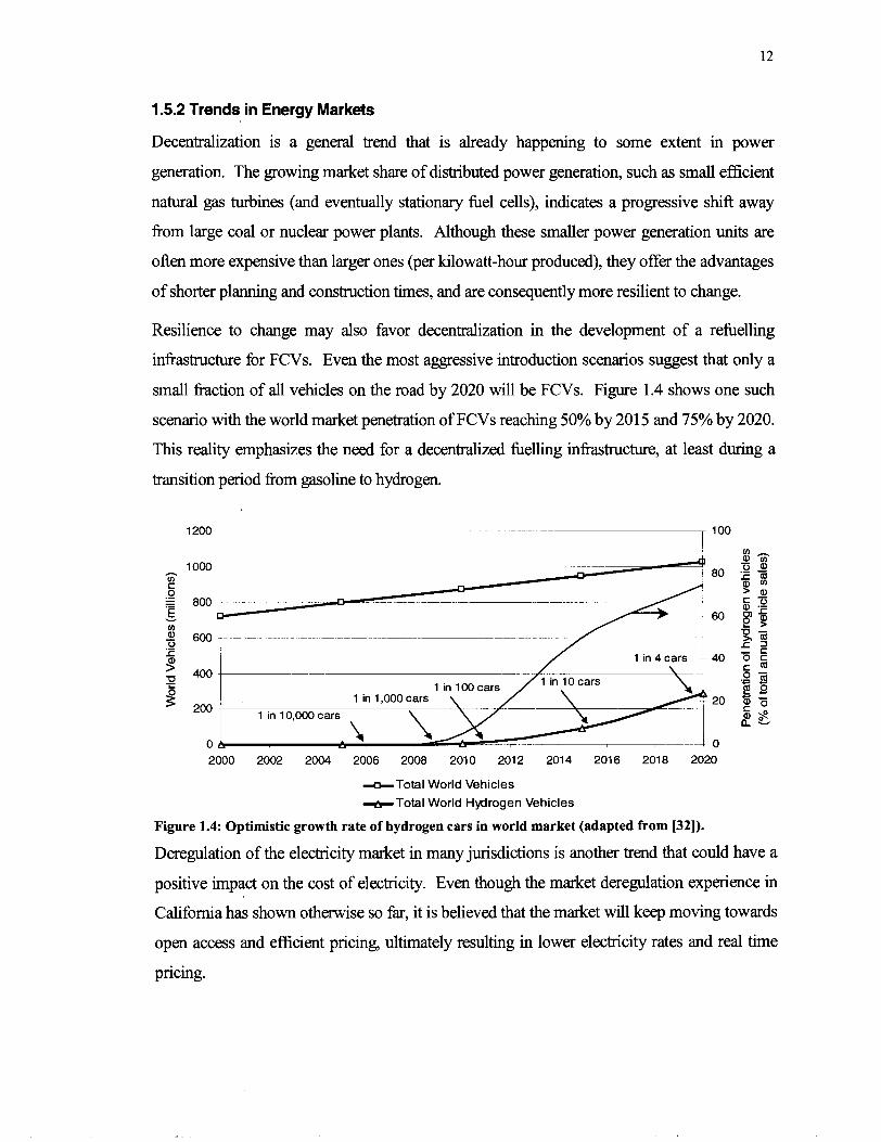
Resilience to change may also favor decentralization in the development of a refbelling
infiastructure for FCVs. Even the most aggressive introduction scenarios suggest that only a
small fiaction of all vehicles on the road by 2020 will be FCVs. Figure 1.4 shows one such
scenario with the world market penetration of FCVs reaching 50% by 201 5 and 75% by 2020.
Thls reality emphasizes the need for a decentralized fbelling infiastructure, at least during a
transition period &om gasoline to hydrogen.
I 1000 --
h V) c 0 .- - - 800
V)
9 600 T - - - -- - . 0
1 in 4 cars - 40 \ .
1 In 1,000 cars
1 In 10,000 cars
2000 2002 2004 2006 2008 2010 2012 2014 2016 2018 2020
&Total World Vehicles
+Total World Hydrogen Vehicles
Figure 1.4: Optimistic growth rate of hydrogen cars in world market (adapted from [32]).
Deregulation of the electricity market in many jurisdictions is another trend that could have a
positive impact on the cost of electricity. Even though the market deregulation experience in
California has shown otherwise so far, it is believed that the market will keep moving towards
open access and efficient pricing, ultimately resulting in lower electricity rates and real time
pricing.

1.5.3 Externalities
Most current means of producing and utilizing energy cause damages to human health, natural
ecosystems, and the built environment, which are difficult to determine, let alone to quantify
in monetary terms. As a result, these damages are either ignored or valued at zero in
traditional financial assessments. They are treated as external costs, i.e. they are not reflected
in the market price of energy. They are part of the "externalities" of energy systems. In
economic theory, externalities are defined as: "the costs and benefits which arise when the
social or economic activities of one group of people have an impact on another, and when the
first group fail to account for their impacts" [33].
The growing public concern with environmental issues has been pushing policymakers to
recognize these external costs of energy. The interest for some new accounting framework
that allows the internalization of externalities has led to "ExternE" - one such framework
jointly developed over several years by the European Commission and the US Department of
Energy (DOE) [33]. The extent to which these externalities (namely the effects of GHG
emissions) will be recognized in coming years will clearly influence business decisions related
to fuel options for future vehicles.
1.5.4 Energy Security
With the growing dependence of the United States, Europe and East Asia on imported oil
fi-om the Middle East, energy security is a factor that could play an important role in the
support for the development of alternative energy sources.
The cost of maintaining a military presence in the Middle East, to ensure stability of the region
and access to oil, is also an economic argument (particularly for the United States) to support
the development of energy systems using indigenous energy sources.
1.6 Focus and Methodology of this Study
This research is focused on decentralized electrolysis, i.e. small refuelling stations that
produce hydrogen on-site to support the needs of 2 to 1000 FCVs, as opposed to large-scale
electrolysis plants. As pointed out earlier, even if FCVs successllly penetrate mass markets,
it is almost certain that hydrogen-fuelled FCVs will represent a minority of vehicles on the
road in most locations for at least the next 20-25 years. During this transitional period,

decentralized hydrogen production could be the most flexible and advantageous option. The
majority of studies done prior to the mid-1990s on the production of electrolytic hydrogen
considered a large-scale centralized approach, similar to the production of gasoline in oil
refineries [34-351. Some of these centralized schemes may prove to be more economical once
FCVs are widespread.
To understand where this technology fits in a broader picture, a basic comprehension of the
architecture of energy systems is helpll. Any energy system can be broken down
conceptually into a five-link chain that goes fiom the service that is needed to the energy
source used to provide it. Even though the direction of the energy flow is fiom the source to
the service, the chain really starts with the service because this is what drives the choices in the
other links of the chain [36] (see figure 1.5 below).
ICE: Internal combustion engine FCS: Fuel cell system SMR: Steam methane reforming e- : Electricitv
I methods I Figure 1.5: Path analyzed in reference to the architecture of energy systems.
In the context of this thesis, the service starting the chain is land transportation. The specific
"service technologies" of interest to provide it are the car and its propulsion system. For the
fuel cell system option, attention is directed at one of the "enera currencies" to fuel it:
hydrogen. Then, among the various "transfomer technologies" capable of delivering this
hydrogen, the focus is on water electrolysis. Since electrolysis necessitates an electricity input
(an intermediate energy currency), multiple enera sources (uranium, wind, sun.. .) can be
used to produce it. Figure 1.5 shows the resulting chain of interest fiom transportation to the

electricity mix. Here, the box "electricity mix" refers to all possible combinations of energy
sources used with the appropriate transformer technologies to generate electricity.
The main objective of this thesis is to provide a tool that will assist not only engineers, but also
business people and policymakers, in directing their actions effectively to improve the
competitive position of electrolytic hydrogen as a fuel. To this end, an analysis fiom three
increasingly broader perspectives is proposed. It starts with the technical aspect, which is
typically the domain of engineers. Then it considers an economic perspective, particularly
financial and market aspects, most relevant to a business outlook. Finally, it addresses what is
called here the "comparative" aspect, i.e. issues like taxes, incentives/subsidies which can
influence the competitive position of a fuel option versus the others. This third aspect is
particularly relevant to policymakers, who can use various tools to catalyze change, and
ensure a level playing field for hydrogen as a fuel option. Figure 1.6 shows a schematic view
of the three perspectives considered in this analysis.
Figure 1.6: Aspects of decentralized water electrolysis investigated.
A more thorough study of any of these three aspects could have justified a thesis of its own,
but the value here lies more in the integration of perspectives and the qualitative conclusions
that can be drawn fiom th~s exercise. In particular, this approach gives the opportunity to
compare the potential impact of different technical improvements, not only between
themselves, but also with issues in the other two aspects considered.
A model was developed in Microsoft Excel to allow the quantitative comparison of actions in
each of the three perspectives. The main parameter of the model is the unit cost of hydrogen
($kg), which is used as a common basis for a sensitivity analysis. The impact of each
parameter is translated in economic terms, affecting the unit cost of hydrogen. The model
developed builds on previous modeling studies, and the base case used for sensitivity analysis

is adapted from previous studies as well. The model's structure is described in details in
Chapter 3, along with its validation procedure.
When electrolyhc hydrogen is compared to other fuel options, comparison is made on a %el-
cost-per-kilometer" basis. This constitutes a better approach than comparison on an energy-
content basis in this case, because the fuel cost per lulometer is what the consumer pays. For
example, even if electrolytic hydrogen costs twice as much as gasoline on an energy-content
basis, the he1 cost per kilometer could be the same if the vehicle's propulsion system is twice
as efficient.
The analysis section proceeds in two steps. First, a sensitivity analysis is performed following
the structure of the cost model, and the parameters are categorized under the technical,
economic or comparative aspect. In the second part of the analysis, the parameters are
grouped and translated into "issues" that influence the price of electrolyhc hydrogen or its
competitive position. Actual data from three different cities is used in that section to illustrate
the impact of site-specific information. Finally, the results of the analysis are discussed and
recommendations are made.
There are obviously some caveats to this study, which should be taken into account when
interpreting the results. They relate to some assumptions made in the context of this research
and inherent limitations of the model. Important ones are listed here:
This study makes comparisons of &el costs only, independently of the capital and
operating costs of the vehicle. In other words, the cost model developed here decouples
the fuel cost from other vehicle costs. In reality, for FCVs to compete with ICE vehicles
on an economic basis, what really matters is that the life-cycle costs of owning and
operating the vehicle be similar. Fuel costs account for approximately 8% or less of the
total cost of owning and operating a car [4]. However, it is very likely that most
consumers would insist on comparable fuel prices at the pump. So consumer behavior is
an important factor to justifl the comparison of fuel costs separately. If the life-cycle costs
of hydrogen-fuelled FCVs are shown to be comparable to those of an ICE vehicle, there
are mechanisms to allow the adjustment of hydrogen prices at a level that satisfies the
consumer.

A theoretical monetary valuation is given to COz to calculate the magnitude of the surtax
or credit assigned to electrolytic hydrogen. This is a convenient simplification to obtain a
first order assessment of the impact of C02. A more representative approach would
require taking into account marginal costs associated with the application of tax/credit
measures: Also, the value assigned to C02 does not have to always reflect the market
price of C02 emissions. For instance, a much higher credit for low CQ emissions granted
initially could accelerate the introduction of FCVs, before getting back to the market price
of C02 emissions, once FCVs have been introduced.
The model and results analysis both present a number of limitations. Several couplings
are not reflected explicitly in the model. For example, a larger electrolyzer station could
possibly benefit fiom lower electricity rates than a smaller one, but this is not accounted
for in the model. Also, the model assumes that an electrolyzer station functions at its
nominal production capacity, which tends to minimize its capital price by amortizing it on
a larger volume of hydrogen than a more realistic case. In the results analysis, the impact
of various issues depends in part on the estimated range of variation for the corresponding
parameters. All these elements are W e r discussed in the analysis portion of Chapter 4.
1.7 Prior Work
At the time this research was started, much valuable work had already been published about
the technical, economic, environmental and social implications of fuel choices for FCVs.
Since then, the growing interest of governments and the private sector for fuel cells has
stimulated a lot more research and thorough studies on these issues. A representative sample
is mentioned here.
1.7.1 Fuel choices for FCVs
Thomas et al. fiom Directed Technologies Inc. (DTI) have performed a substantial amount of
work on he1 options for FCVs, mostly during the second half of the 1990ts, under contract
with the US Department of Energy (DOE) [4,37-381. The overall results emerging from their
work seem to be that onboard hydrogen is the preferred fuel option for FCVs, and that
hydrogen produced fiom natural gas reforming (small-scale SMR) presents the most
interesting opportunity. In fact, some directors at DTI later started a company called H2Gen,
whose main product is a small-scale SMR [39].

Another group that has been active for several years in he1 infi-astructure issues for FCVs is
the Center for Energy and Environmental Studies led by Joan M. Ogden at Princeton
University. They have covered a wide array of issues related to a hydrogen fuel infrastructure
[29,4O].
Organizations such as the California Fuel Cell Partnership (CaFCP) in the United States and
the Canadian Transportation Fuel Cell Alliance (CTFCA) in Canada have contributed to the
literature on the subject, with several reports fi-om expert panels. One of these reports written
in 2001 for the CaFCP provides exhaustive information on the options of hydrogen, methanol,
gasoline and ethanol fuel [3 11. A more recent report produced by Ernst & Young for Natural
Resources Canada in 2003 concludes that multiple hydrogen pathways in Canada could
compete economically with gasoline and diesel, with a combination of emission taxes and
excise tax exemptions [4 1 1.
Finally, a comprehensive study conducted in 2001 by General Motors, Argonne National
Laboratory and energy partners BP, ExxonMobil and Shell, concluded that gasoline or a
gasoline-derived fuel is the best option for FCVs in the near-term and that hydrogen is clearly
the preferred option for the long-term. The study covered 75 fuel pathways and reinforced
GM's philosophy that there is no need for an intermediate fuel infi-astructure such as methanol
or compressed natural gas [Ill.
1.7.2 The Electrolysis Option
The Electrolyser Corporation (now Stuart Energy Systems) produced a substantial report for
the Ford Motor Company in 1996, focusing on the electrolysis option for the FCV fuel supply
infi-astructure. The report covers a broad range of issues fi-om electricity supply strategies to
safety analysis of FCV fuelling stations [42].
Another report by DTI for the National Renewable Energy Laboratory (NREL) investigated
the electrolytic hydrogen option and analyzed the potential for low-cost electricity in the
United States. The study showed that there is potential for electrolytic hydrogen to compete
with gasoline in many parts of the country, based on off-peak electricity rates [43].

Several studies that have been reviewed look at the possible integration of renewable energy
sources with water electrolysis or other technologies to produce hydrogen. Mann et al. fiom
NREL are a noteworthy reference for literature on the production of hydrogen fiom renewable
resources [44].
1.7.3 The Influence of Greenhouse Gas Emissions
In light of the implications of the Kyoto Protocol and the issue of GHG emissions in the long-
term, a lot of work has been done on well-to-wheel GHG emissions fi-om the various fuel
pathways. Most of the studies mentioned in the prior work section about fuel choices (1.7.1)
address the GHG issue.
Two studies produced in Canada on the subject are particularly thorough [45-461. The first
one was produced by the Pembina Institute for Appropriate Development and presents a
detailed assessment of the life-cycle value of fuel supply options for FCVs in Canada. The
second one, prepared for Fuel Cells Canada, used Natural Resources Canada's model called
"GHGenius" to analyze the life-cycle energy use and GHG emissions of fifty fuel pathways
for transportation. Both studies emphasize the wide range of GHG emissions that can result
fiom different hydrogen production pathways, fi-om much lower to much higher GHG
emissions than gasoline used in ICE vehicles.
Energy companies like Shell, BP and ExxonMobil have also participated to some studies of
GHG emissions fiom various fuel options, or produced their own [30,47]. They all recognize
the potential of hydrogen fuel to reduce GHG emissions substantially, but only in a limited set
of production pathways.

Chapter 2 - Water Electrolysis
Background
2.1 Principles
The production of hydrogen by the electrolysis of water is, in principle, very simple. It is a
process by which electricity is used to decompose water into its components - gaseous
hydrogen and oxygen. The overall reaction is:
H,O + energy 2 H, + 0, (2.1)
A typical electrolysis cell' is composed of two electronic conductors (a positively charged
electrode - the anode, and a negatively charged electrode - the cathode) in contact with an
ionic conductor, the electrolyte. When an electric direct current (DC) is passed through such a
cell containing water, the water molecules may be split into hydrogen and oxygen. The
voltage required to "pump" the electrons (e-) that make up th~s direct current is largely
determined by thermodynamic considerations. The principles of an electrolysis cell are shown
in figure 2.1 for an alkaline electrolyte.
Figure 2.1: Principle of alkaline water electrolysis (AWE).
1 A cell commonly refers to the basic elements making up a single electrochemical circuit.

Although the discovery of electrolytic water splitting was done in an acidic solution, alkaline
electrolytes have been prefmed in actual applications, mainly because of lesser corrosion
problems. Large-scale electrolyzers commercialized during the twentieth century are all based
on conventional alkaline water electrolysis (AWE). However, other promising types of
electrolyte exist like those used for solid polymer electrolysis (SPE) and high temperature
electrolysis (HTE). The basic principles and reactions for each of these three types of
electrolyte are presented below.
2.1.1 Alkaline Water Electrolysis (AWE)
Since water is a very poor ionic conductor, the electrolyte has to contain other components to
obtain a reasonable conductivity. For alkaline electrolysis, potassium hydroxide (KOH) is the
most used component given its good conductivity. The KOH electrolyte typically has a
concentration of 25-30% (by weight). In conventional AWE, electrolysis takes place at a
temperature around 80 OC and a pressure in the range of 1 to 30 bar [22], although higher
temperatures and pressures can now be achieved with advanced AWE technology.
The basic reactions at the two electrodes are given below with a net overall reaction equivalent
to reaction 2.1.
Cathode: 2H,O + 2e- 3 H, + 20H- (2.2)
Anode: 20H- 3 3 0 , + H 2 0 + 2 e - (2.3)
Overall reaction: H, 0 3 H , + 4 0,
Using a KOH solution as an example (and adjusting the stoichiometric coefficients to see the
net reaction more clearly), the reaction at the cathode proceeds as follows:
Net cathode reaction: 2 H , 0 + 2e- H , + 20H -

The reaction is initiated when positively charged potassium ions are reduced (reaction 2.4) and
subsequently react with water to form hydrogen atoms and hydroxyl ions (reaction 2.5). The
highly reactive hydrogen atoms then bond to the metal of the cathode. Hydrogen atoms
combine in pairs at the surface of the cathode to form hydrogen molecules, which leave the
electrode as a gas (reaction 2.6) [48]. As expected, the net cathode reaction is identical to
reaction 2.2.
At the anode, a reaction similar to the one at the cathode occurs, producing oxygen:
20H- =, 20H + 2e- (2.7)
2 0 H = H,O+O (2.8)
1 0 + + 0 + 0 2 2 (2.9)
Net anode reaction: 20H- a 0, + Hz 0 + 2e-
The net result of sub-reactions 2.7,2.8 and 2.9 is identical to the anode reaction 2.3. Oxygen
molecules are released as a gas at the anode, just like hydrogen at the cathode.
For AWE to proceed steadily, hydroxyl ions (OH-) must continuously migrate fiom the
cathode to the anode, in a way that prevents the intermixing of hydrogen and oxygen. To this
end, a separator (diaphragm or membrane) is placed between the electrodes. This separator
must allow the fiee passage of ions, while acting as a banier to keep the gases apart (see figure
2.1).
Catalysts are applied to the surface of the electrodes to increase the recombination rates of
atomic hydrogen and oxygen. Without a catalflc coating, atomic hydrogen would build up
on the cathode surface, hence reducing the current flow and slowing the production of
hydrogen gas. The effectiveness of the catalytic coatings is improved by increasing the ratio
of real to apparent surface area of an electrode. A high porosity is therefore desirable for the
electrode surfaces.
In AWE, water is generally fed to the circulating electrolyte, which also provides a convenient
way to remove the waste heat produced by the electrolysis reaction and control the process
temperature.

2.1.2 Solid Polymer Electrolysis (SPE)
In SPE, a solid rather than liquid electrolyte is used. While acid solutions are not used today
in practical water electrolysis, acid membranes offer an interesting alternative to liquid
alkaline electrolytes. Acid membranes used in SPE are of the same type as those used in
proton exchhge membrane fuel cells (PEMFC). Their main feature is a high proton
conductivity and a very low electronic conductivity. In other words, they allow the migration
of protons (or more accurately hydroxonium ions - ~~0': a proton attached to a water
molecule) between the electrodes, while preventing electrons to go through the same path.
Electrons have to pass by an external circuit to go fkom one electrode to the other. The
principles of SPE are illustrated in figure 2.2.
Figure 2.2: Principle of solid polymer electrolysis (SPE).
The reactions taking place at each of the electrodes in SPE are different from the reactions in
AWE, but the overall water-splitting reaction is the same.
Cathode: 2H,O' + 2e- 2H,O + H ,
Anode: 3H20 2H,O' +2e- +3O,
Overall reaction: H,O 3 H , +3O,

Water is decomposed electrochemically at the anode in oxygen gas, hydroxonium ions ( ~ 3 0 3
and electrons (reaction 2.1 1). The hydroxonium ions then migrate through the membrane and
recombine with electrons, which pass via an external circuit, to form hydrogen gas and water
at the cathode (reaction 2.1 0).
The polymer membranes used in SPE serve both the roles of electrolyte and separator. Most
membrane materials are based on "sulphonated" fluoropolymers to conduct protons. PTFE
(polytetrafluoroethylene, also known commercially as ~eflon? is the fluoropolymer normally
used in SPE membranes. PTFE is created by substituting fluorine for the hydrogen in a
polyethylene polymer. The basic PTFE polymer is then "sulphonated", i.e. side chains are
added, ending with sulphonic acid HS03. An example of a side chain structure attached to
PTFE is shown in figure 2.3 [49]. The most well known membrane material for both SPE and
PEM fuel cells is ~ a f i o n ~ , which has been developed by DuPont through several variants
since the 1960's.
Figure 2.3: Example structure of a sulphonated fluoropolymer [49].
The HS03 goup is ionically bonded, so the end of each side chain is actually an SO3- ion.
The presence of S 0 i and Hf ions results in strong mutual attraction between the + and - ions
fiom each side chain molecule, thus creating "clusters" of sulphonic acid within the material.
A key property of sulphonic acid is that it is highly hydrophyllic - it attracts water; PTFE on
the other hand is hydrophobic - it repels water. The hydrophyllic regions around the clusters
can absorb relatively large amounts of water (increasing the dry weight of the membrane by
up to 50%). Within these hydrated regions, the H+ ions (protons) are relatively free to move,

thus creating a dilute acid. Between the hydrated regions, it is still possible for H+ ions to
migrate short distances through the supporting long molecule structure, albeit with more
difficulty. A well-hydrated membrane is therefore key to promote the flow of protons and the
overall electrolysis reaction rate. Protons crossing the membrane electrolyte drag water
molecules with them, which explains the appearance of hydroxonium ions ( ~ ~ 0 3 in reactions
2.10 and2.11.
Each electrode is usually made of a thin layer of carbon-supported platinum catalyst, bonded
to the membrane electrolyte. Platinum is still considered to be the best catalyst for both the
anode and cathode; but the amount required for SPE has been considerably reduced over the
last decade (below 1 mg of platinum per cm2 of membrane), largely due to advances in PEM
fuel cell technology.
The upper temperature limit of the fluoropolymer membrane material is around 125-150 O C ,
however most SPE electrolyzers operate on liquid water at a temperature of 80 O C [22].
Higher operating temperatures could be achieved with new polymer membrane materials or
even ceramic proton-conducting materials. At these higher temperatures, water is present as
steam when it undergoes the electrolysis reaction. To remove the waste heat generated by
SPE electrolysis, the feed water is generally circulated at a sufficient rate over the anode side
[231.
One of the advantages of SPE is the capacity to operate at higher current density than AWE.
For instance, SPE can operate at over 90% energy efficiency at a current density of 1-2 A/cm2
[50-511. This compares to a current density of about 0.3 A/cm2 used in AWE to obtain a
similar energy efficiency [52-531. In other words, in spite of higher material costs, an SPE
electrolyzer would require only a fraction of the cell area required in an AWE electrolyzer to
produce hydrogen at the same rate and high efficiency.
Finally, the compact design of SPE electrolyzers (each cell is only a few millimeters thick) is
well suited for high pressure electrolysis. SPE electrolyzers with operational pressures up to
20 MPa (3000 psi) are currently used for US Navy submarine oxygen generators [54].

2.1.3 High Temperature Electrolysis (HTE)
HTE takes place at much higher temperatures than AWE or SPE, typically in the 900-1 000 OC
range, and water is fed as steam. The electrolyte is made of a solid ceramic material that
conducts oxygen ions. The high operating temperature is necessary for ceramics to offer a
satisfactory ionic conductivity. Vapour-phase electrolysis is also desirable fiom a
thermodynamic perspective, as it allows a greater portion of the required energy to come fiom
heat instead of electricity (see section 2.2.1 : Thermodynamics).
Just like SPE is essentially a PEM he1 cell operating in reverse, HTE relies on the same
chemistry and materials as a solid oxide fuel cell (SOFC). The ceramic solid electrolyte
allows oxygen ions to migrate fiom the cathode to the anode, while electrons have to move via
an external circuit to go fiom the anode to the cathode. The ceramic electrolyte also acts as a
gas separator. The principles of HTE are illustrated in figure 2.4.
Cunent collector Current collector
Cathode -
Oxygen ion conducting electrolyte
Figure 2.4: Principles of high temperature electrolysis (HTE).
Once again, the basic reactions taking place at the electrodes are different fiom those in AWE
or SPE, but the overall water-splitting reaction remains the same.
Cathode: H,O + 2e- 3 H, + 0'- (2.12)
Anode: 0'- 3 to2 + 2e- (2.13)
Overall reaction: H , O ~ H , +30,

Vaporized water is fed to the cathode chamber where it reacts with electrons to be split into
hydrogen and oxygen ions (reaction 2.12). A h migrating to the anode, the oxygen ions then
release electrons and combine in pairs to create oxygen gas (reaction 2.13).
2.1.4 Basic Electrolyzer Configurations
Industrial electrolyzers are composed of multiple electrolysis cells or electrode pairs, which
may be connected in parallel or in series. There are two primary electrolyzer configurations
commonly known as the tank type (or monopolar) and the filter-press type (or bipolar).
In a tank electrolyzer, each individual electrode is fed current fiom outside and has a single
polarity (monopolar), i.e. it is either a cathode or an anode. The cells within a tank are
connected in parallel as shown in figure 2.5. The voltage across the whole tank is the same as
the voltage across any individual cell, ECel1 (typically 1.5-2 Volts), irrespective of the number
of electrode pairs in the tank.
Diaphragm Figure 2.5: Principles of a tank electrolyzer (monopolar).
+ l-
Figure 2.6: Principles of a filter-press electrolyzer (bipolar)
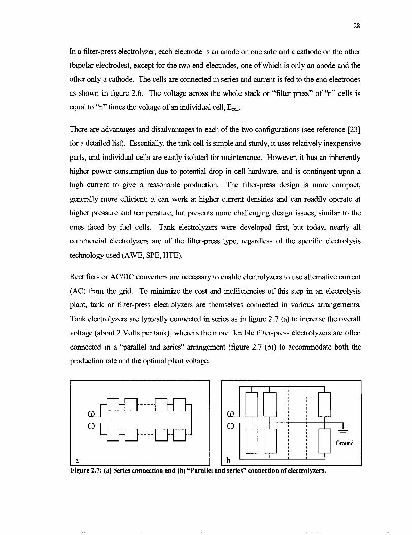
In a filter-press electrolyzer, each electrode is an anode on one side and a cathode on the other
(bipolar electrodes), except for the two end electrodes, one of whch is only an anode and the
other only a cathode. The cells are connected in series and current is fed to the end electrodes
as shown in figure 2.6. The voltage across the whole stack or "filter press" of "n" cells is
equal to "n" times the voltage of an individual cell, ECel1.
There are advantages and disadvantages to each of the two configurations (see reference [23]
for a detailed list). Essentially, the tank cell is simple and sturdy, it uses relatively inexpensive
parts, and individual cells are easily isolated for maintenance. However, it has an inherently
higher power consumption due to potential drop in cell hardware, and is contingent upon a
high current to give a reasonable production. The filter-press design is more compact,
generally more efficient; it can work at higher current densities and can readily operate at
higher pressure and temperature, but presents more challenging design issues, similar to the
ones faced by he1 cells. Tank electrolyzers were developed first, but today, nearly all
commercial electrolyzers are of the filter-press type, regardless of the specific electrolysis
technology used (AWE, SPE, HTE).
Rectifiers or ACDC converters are necessary to enable electrolyzers to use alternative current
(AC) fi-om the grid. To minimize the cost and inefficiencies of this step in an electrolysis
plant, tank or filter-press electrolyzers are themselves connected in various arrangements.
Tank electrolyzers are typically connected in series as in figure 2.7 (a) to increase the overall
voltage (about 2 Volts p a tank), whereas the more flexible filter-press electrolyzers are often
connected in a "parallel and series" arrangement (figure 2.7 (b)) to accommodate both the
production rate and the optimal plant voltage.
Figure 2.7: (a) Series connection and (b) "Paralh and series" connection of electrolyzers.

2.2 Energy Use
Previous techno-economic studies show that electricity is nearly always the largest component
of electrolytic hydrogen cost, typically accounting for more than 50%, and as much as 80% of
its cost [28,55]. It is therefore fundamental to understand the physical limitations of water
electrolysis in terms of energy use, to get an appreciation of the room for potential
improvements.
2.2.1 Thermodynamics
The net water-splitting reaction is, as stated before:
Since this net reaction is the same for AWE, SPE and HTE, the thermodynamic aspects are
identical for all of these water electrolysis technologies [23].
A simplified process diagram shows the material and energy flows in standard electrolysis
(figure 2.8). Pure water enters the system; hydrogen and oxygen leave it. Electricity is
supplied to the system; heat is removed fiom and/or supplied to it.
Electricity
Heat Figure 2.8: Simplified process diagram for hydrogen production by water electrolysis.
The energy change of reaction 2.14, i.e. the theoretical energy required for the reaction to
proceed, can be expressed through the following thermodynamic equation:
where AH is the enthalpy change of the reaction, AG is the Gibbs free energy change, T is the
absolute temperature and AS is the entropy change [48].

The Gibbs fiee energy change AG corresponds to the portion of the total reaction energy that
must be supplied in the form of electricity, when water splitting is performed by electrolysis.
The term "TAS" corresponds to the portion of the total reaction energy that could
thermodynamically be covered by thermal energy.
Under standard temperature and pressure conditions (STP' - indicated below by superscript O),
the enthalpy change of reaction 2.14 based on liquid water is
AH:,,, = 285.8 kJ/mol
This value also corresponds to the so-called higher heating value (HHV) of hydrogen, which
is the theoretical amount of energy released when pure hydrogen is combusted completely
with oxygen, and water appears as a liquid in the products of combustion.
The corresponding change in Gibbs fiee energy at STP is
AG:,,, = 237.2 Wmol
In other words, 237.2 out of 285.8 Wmol, or 83% of the minimum energy required to
electrolyze liquid water under standard conditions must come from electricity. The other 17%
could theoretically be supplied by heat or by electricity as well.
In practice, electricity provides all of the energy theoretically required by a low-temperature
electrolysis cell (e.g. 80 O C ) , and some more to overcome various losses. The result of these
inefficiencies is waste heat that must be dissipated. However, it is possible to have heat
provide part of the energy required at higher temperatures. It is even conceivable that an
extremely well performing low-temperature electrolyzer could use heat from its surroundings
to provide a small portion of the energy required, in which case the electrolyzer would act as a
refhgerator [56]. Such an electrolyzer is hghly unlikely though.
Two distinct cell voltages can be calculated from the change in Gibbs free energy AG and the
reaction enthalpy AH. The first one is called the reversible voltage, bV, and is given by:
1 Standard temperature and pressure or standard reference state, i.e. 25 "C (298.15 K) and 1 bar.

where F is the Faraday constant. It corresponds to the minimum electrical potential needed to
drive the electrolysis reaction. At STP, kV has a value of 1.23 Volts.
The voltage associated with AH is commonly called the thermoneutral cell voltage, &. It is
the voltage at which a perfectly efficient cell would operate if electricity provided the entire
energy requirement. Under these conditions, the cell does not generate any waste heat, nor
does it require any heat input; the cell has no net heat exchange, hence it is then said to be
"thermoneutral". At STP, & has a value of 1.48 Volts.
To summarize, if an electrolysis cell operates below the reversible voltage &, no sustained
water splitting can occur. If it operates between bV and the thermoneutral voltage &, then
the process is endothermic and part of the energy required to split water comes fi-om heat. If it
operates above &, the process is exothermic, meaning that excess heat must be dissipated,
and all of the energy required comes fi-om electricity.
AH and AG, and consequently & and b,,, are functions of the temperature, pressure and
electrolyte composition.
Equations 2.1 6 and 2.1 7, which link energy and voltages, can be derived easily. As indicated
in the previous section, two electrons must pass round the external circuit to split each water
molecule. So, for one mole of hydrogen produced, 2N electrons must pass round the external
circuit (where N is Avogadro's number). If -e is the charge on one electron, then the charge
that flows is:
- 2 Ne = -2F Coulombs
F being the Faraday constant.
If E is the actual voltage of an electrolysis cell, then the electrical work done by the
electrolyzer, moving this charge round the circuit is:
Electrical work done = charge x voltage = - 2F.E Joules
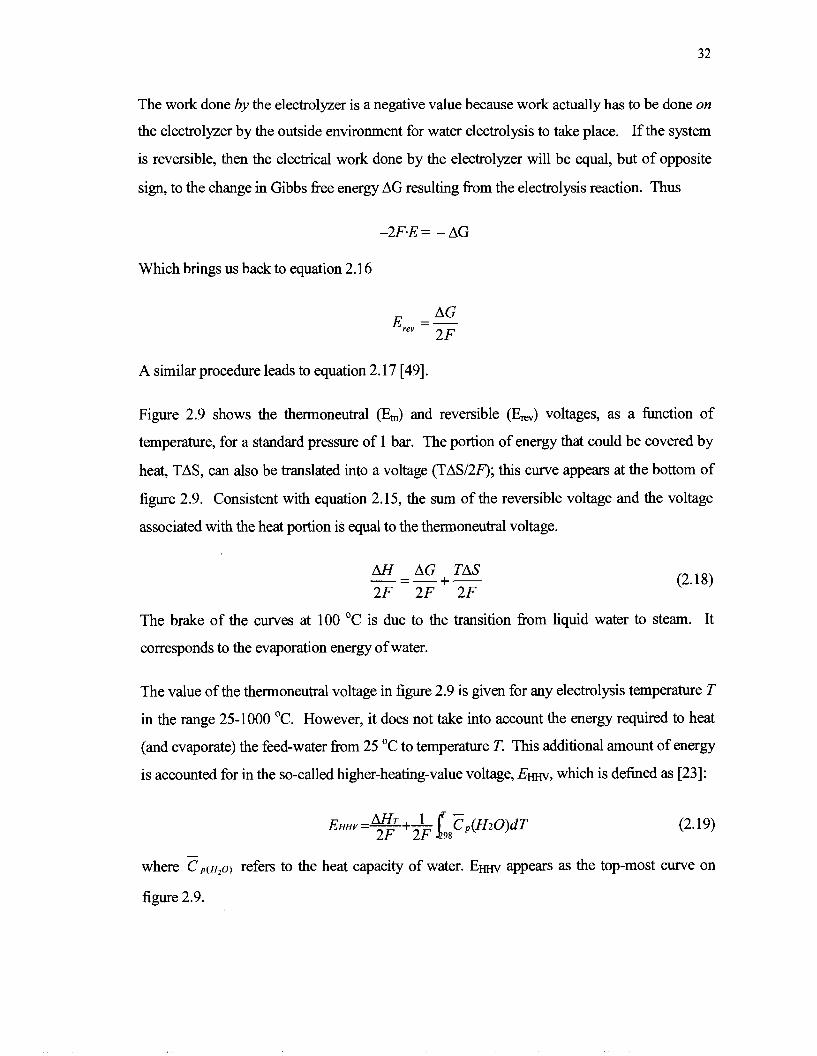
The work done by the electrolyzer is a negative value because work actually has to be done on
the electrolyzer by the outside environment for water electrolysis to take place. If the system
is reversible, then the electrical work done by the electrolyzer will be equal, but of opposite
sign, to the change in Gibbs fiee energy AG resulting fiom the electrolysis reaction. Thus
Which brings us back to equation 2.16
A similar procedure leads to equation 2.17 [49].
Figure 2.9 shows the thermoneutral (b) and reversible (&) voltages, as a function of
temperature, for a standard pressure of 1 bar. The portion of energy that could be covered by
heat, TAS, can also be translated into a voltage (TASI2F); th~s curve appears at the bottom of
figure 2.9. Consistent with equation 2.15, the sum of the reversible voltage and the voltage
associated with the heat portion is equal to the thermoneutral voltage.
AH AG TAS - +- (2.1 8)
2 F 2 F 2 F
The brake of the curves at 100 O C is due to the transition fkom liquid water to steam. It
corresponds to the evaporation energy of water.
The value of the thermoneutral voltage in figure 2.9 is given for any electrolysis temperature T
in the range 25-1000 O C . However, it does not take into account the energy required to heat
(and evaporate) the feed-water fkom 25 "C to temperature T. This additional amount of energy
is accounted for in the so-called higher-heating-value voltage, E m , which is defined as [23]:
- where Cp(H,o) refers to the heat capacity of water. Em appears as the top-most curve on
figure 2.9.

As illustrated in figure 2.9, the reversible voltage LV decreases significantly from 1.23 Volts
at 25 OC (298 K) to 0.92 Volt at 1000 OC (1273 K). It means the amount of electrical energy
needed to perform electrolysis is reduced at higher operational temperatures. The
thermoneutral voltage E, remains relatively constant though (except for the drop associated
with water vaporization), while the higher-heating-value voltage Em grows steadily fiom
1.48 Volts at 25 "C to 1.72 Volts at 1000 OC.
In other words, although the energy required to electrolyze water as such is relatively constant,
as indicated by the thermoneutral voltage, the portion that has to be supplied by electricity
decreases as a function of temperature, as indicated by the reversible voltage. In fact, the
electricity requirement decreases by 25% (fiom 1.23 V to 0.92 V) between 25 OC and 1000 "C.
On the other hand, the higher-heating-value voltage clearly increases with temperature as a
result of the greater energy needed to bring the feed water to the operating temperature.
Tern pera ture (K)
Figure 2.9: Theoretical water electrolysis voltages as a function of temperature.
Appendix A gives more detailed information on the thermodynamics of water electrolysis and
the data used to generate the graph of figure 2.9.
2.2.2 Efficiencies
There is some confbsion in the literature about the various efficiencies of water electrolysis.
Different authors talk about efficiency, energy efficiency, electrical efficiency, current
efficiency, electrochemical efficiency, exergy efficiency [22,48,50,56,57,58]; sometimes at
the cell level, and sometimes at the electrolyzer system level (including ACIDC conversion,
etc.).
Probably the most general definition of the energy efficiency of the electrolysis process is
given as [5 81 :
Energy output in products Energy efficiency =
Total energy input
In the case of conventional water electrolysis, the energy input is limited to electrical energy.
Hence, the energy efficiency of an electrolyzer has traditionally been defined as "the energy
that ideally could be recovered by reoxidation of the hydrogen and oxygen coproducts to
water (the heating value of hydrogen), divided by the energy supplied to the electrolysis
system in electrical form" [57].
Heating value of hydrogen output Energy efficiency = (2.20)
Energy of electrical input
Some references use the lower heating value (LHV) of hydrogen while others use its higher
heating value (HHV) to calculate the energy efficiency of electrolysis. In this research, the
HHV value is always the one used, as it better reflects the fbll energy content of hydrogen.
Because this last definition disregards thermal energy inputs, the energy efficiency could reach
values above 100%. For instance, in the case where an electrolyzer operates below the
thermoneutral voltage, some heat fi-om the surroundings is used as an energy input, without
being considered in the definition above.
At the cell level, when electricity is the only energy source, the energy efficiency of the
electrolysis process could be defined as the ratio of the thermoneutral voltage (for liquid water
at STP - 1.48 Volts - E, 298, $ to the actual cell voltage (E) [22], multiplied by the current
efficiency [50].

Energy efficiency = Etn,298,L x Current efJiciency E
The current efficiency is simply the ratio of the number of electrons theoretically required to
produce a given amount of hydrogen over the actual number of electrons supplied by the
electrical current in producing this amount of hydrogen (equation 2.22). As mentioned earlier,
two electrons are required for each molecule of hydrogen produced.
Volume of generated H , (Nm3 1 h) x 96,487 (C lmol e ) x 2(mol e - Imol H , ) (2 22) Current eficiency =
Current ( A ) x 3,600 ( s / h) x 0.0224 (Nm3 / mol H,)
Current efficiency is typically around 99%, whereas the energy efficiency as defined in
equation 2.21 varies more widely in the 75-95% range, depending on the particular
electrolysis technology and operating conditions. The 75-95% range is also representative of
actual energy efficiency values according to the definition of equation 2.20, based on the HHV
value of the hydrogen produced. The corresponding range when the LHV value of hydrogen
is used is 63-80%.
These relatively high efficiency values are based on electricity as the energy source.
However, if we consider electricity as an energy currency derived fiom another energy source
(e.g. coal, natural gas, etc.) the overall efficiency of hydrogen production by electrolysis can
drop dramatically, down to the 30% range. Rosen and Scott have proposed a simple
methodology to evaluate the energy and exergy efficiency of water electrolysis in a way that
allows straightforward and relevant comparison with other hydrogen production processes
[58,59,60].
The particular efficiencies used for the cost model are dehed and explained in Chapter 3.
2.2.3 Cell Voltage
The power consumption of an electrolysis cell is directly proportional to the cell voltage and
inversely proportional to its current efficiency. Since current efficiency is usually very close
to loo%, the parameter of importance in evaluating water electrolysis cells design is the
magnitude of the cell voltage.

Water electrolysis under actual conditions demands a cell voltage E that is substantially higher
than the reversible value Em, It has to overcome the electrical resistance in the electrodes, in
the electrolyte between the electrodes, and in the separator. Additionally, it has to cover the
so-called overpotentials at the electrodes, which are kinetically determined. The cell voltage
can then be expressed as [22]:
E = E,, + 7, + qa + jR*
where q, is the cathodic overpotential (hydrogen overvoltage), q, is the anodic overpotential
(oxygen overpotential), j is the current density and R* is the sum of the electrical resistances,
based upon the active electrode area.
Figure 2.10 shows an example of the relations between voltages and current density in
conventional alkaline electrolysis. The cell voltage increases with current density, the ohmic
resistance portion following a linear progression. An example of actual values is given in
table 2.1, referring to an industrial electrolyzer using alkaline electrolyte at common
conditions (25% KOH electrolyte, 80 O C , 1 bar) [22].
Figure 2.10: Voltage vs. current density relationships.
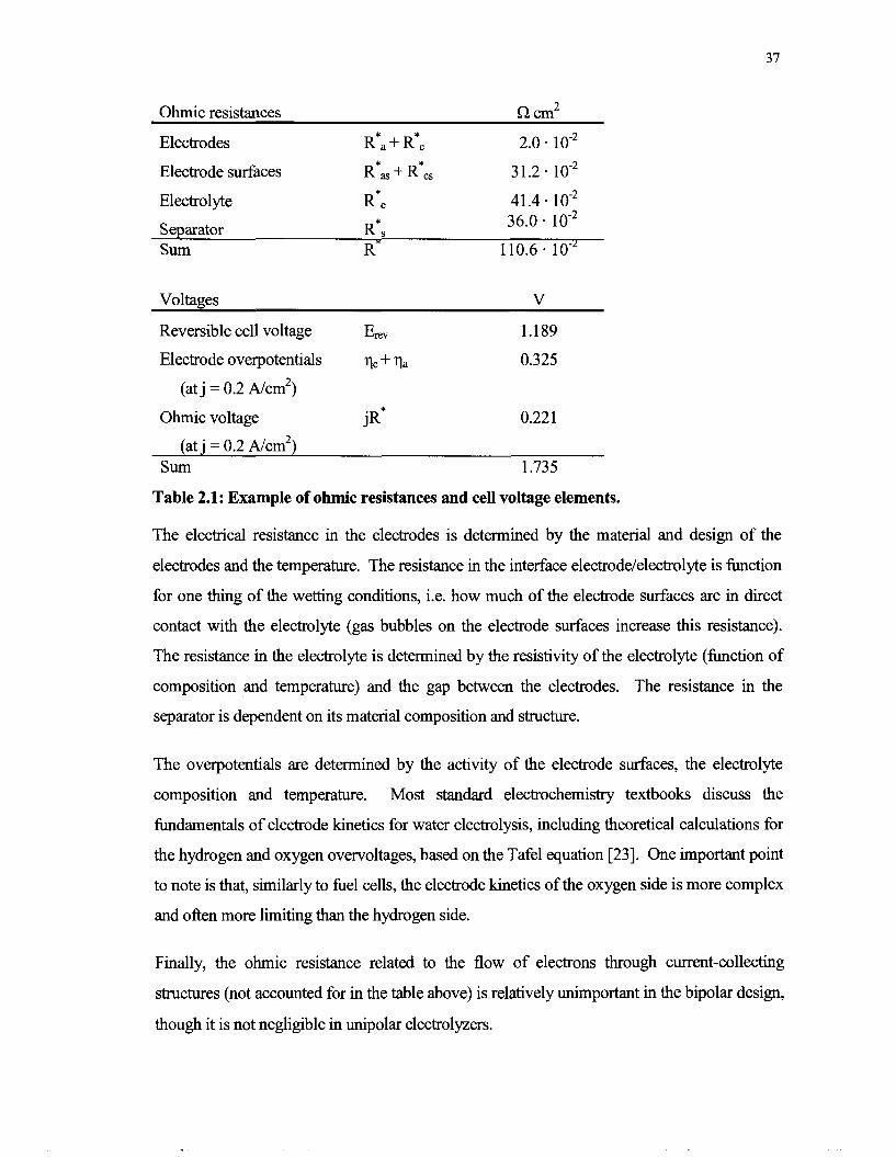
Ohmic resistances Q cm2
Electrodes R * ~ + R * ~ 2.0 lo-2
Electrode sw?gces R * ~ ~ + R * ~ ~ 31.2.
Electrolyte R*, 41.4 . 10"
Separator R*S 36.0 . lo-'
Sum R* 110.6 . lo-'
Voltages V
Reversible cell voltage Em 1.189
Electrode overpotentials qc + va 0.325
(at j = 0.2 Ncm2)
Ohmic voltage jR* 0.22 1
(at j = 0.2 A/cm2) Sum 1.735
Table 2.1: Example of ohmic resistances and cell voltage elements.
The electrical resistance in the electrodes is determined by the material and design of the
electrodes and the temperature. The resistance in the interface electrode/electrolyte is function
for one thing of the wetting conditions, i.e. how much of the electrode surfaces are in direct
contact with the electrolyte (gas bubbles on the electrode surfaces increase this resistance).
The resistance in the electrolyte is determined by the resistivity of the electrolyte (function of
composition and temperature) and the gap between the electrodes. The resistance in the
separator is dependent on its material composition and structure.
The overpotentials are determined by the activity of the electrode surfaces, the electrolyte
composition and temperature. Most standard electrochemistry textbooks discuss the
fundamentals of electrode kinetics for water electrolysis, including theoretical calculations for
the hydrogen and oxygen overvoltages, based on the Tafel equation [23]. One important point
to note is that, similarly to he1 cells, the electrode kinetics of the oxygen side is more complex
and often more limiting than the hydrogen side.
Finally, the ohmic resistance related to the flow of electrons through current-collecting
structures (not accounted for in the table above) is relatively unimportant in the bipolar design,
though it is not negligible in unipolar electrolyzers.
2.2.4 Effect of Operating Conditions
2.2.4.1 Temperature
As illustrated in figure 2.9, increasing the electrolysis temperature reduces the reversible
voltage L V , and therefore the minimum electrical energy input. Quantitatively, it shows that
there is a potential for reducing the minimum electrical input by about 25%, when temperature
is increased from 25 OC to 1000 O C .
Yet, the overall theoretical amount of energy required to perform electrolysis at high
temperature is not lower, but rather slightly higher as indicated by the higher-heating-value
voltage EHHV in figure 2.9.
What higher temperature electrolysis has to offer then is more flexibility to use heat as an
energy input, and increased efficiency due to improved kinetics. When available, heat is
generally cheaper than electricity, and sometimes even free if the electrolyzer is located near
an existing heat source (e.g. nuclear reactor).
2.2.4.2 Pressure
The electrolysis pressure also has an effect on the energy requirement for producing
electrolytic hydrogen. The reversible voltage for a given temperature T and pressure P
(Ere,Tp) can be calculated •’tom the Nernst equation as:
where R denotes the universal gas constant, n the number of electrons to split each water
molecule (n = 2), F the Faraday constant, and a the activity of a species [23]. Erev,rP=l is the
reversible voltage at temperature T (in Kelvin) and standard pressure P = 1 bar. Its value is
given by the curve beV on figure 2.9. The exponent of each activity a corresponds to the
species coefficient in the water splitting reaction (reaction 2.14).
The activities of hydrogen (aH2 ) and oxygen (aq ) can be approximated by their respective
pressure ratio to atmospheric pressure (PH2/P0) and (P02/Po). Because during electrolysis the
pressure is normally the same on the oxygen side and the hydrogen side, we can assume that

P H ~ = Po2 = P. The numerator of activities in equation 2.24 then becomes simply @/Po) 'I2.
The activity of water ( aH2 , ) can be approximated as 1. Assuming Po = 1 bar, equation 2.24
becomes:
with P expressed in bar.
A more comprehensive explanation is given in reference [23]. An alternative approach based
on thermodynamics and the perfect gas law also leads to the same result.
At T = 298 K, equation 2.25 predicts a voltage increase of about 44 mV at 10 bar (- 150 psi),
88 mV at 100 bar (- 1500 psi) and 115 mV at 400 bar (- 6000 psi). For example, an
electrolyzer operating with 10 bar output at 1.55 V might need only 1.62 V to operate at 400
bar, based on theoretical considerations. (1.55 V + (1 15 mV - 44 mV) = 1.62 V)
Although high pressure increases the theoretical reversible voltage by a few percents, it can
generally be justified in actual electrolyzers by the energy saving due to increased efficiency
(reduced operating voltage) and higher achievable current density [56]. For instance, one
effect of high pressure is to reduce the size of gas bubbles on the electrode surfaces, hence
improving the cell performance [23]. So there seems to be an optimum pressure level (which
varies with the particular electrolysis technology used) for which the advantages outweigh the
slight increase in the theoretical voltage.
Now, the principal interest in high-pressure operation is to save the cost of compressing
hydrogen after it is produced [61]. Assuming that gaseous hydrogen is stored onboard FCVs
at high pressure, say 350 bar (- 5000 psi), a compressor must bring it to an even higher
pressure at the helling station, say 400 bar (- 6000 psi). Equation 2.25 indicates that in
theory, the electrolyzer itself could provide the high pressure with a relatively small penalty on
energy use. The small drop in energy efficiency might then justify the elimination of the
compressor from the reheling system. However, very high pressures up to 400 bar would
most likely place severe mechanical constraints on the electrolyzer [43] and increase its capital
cost.
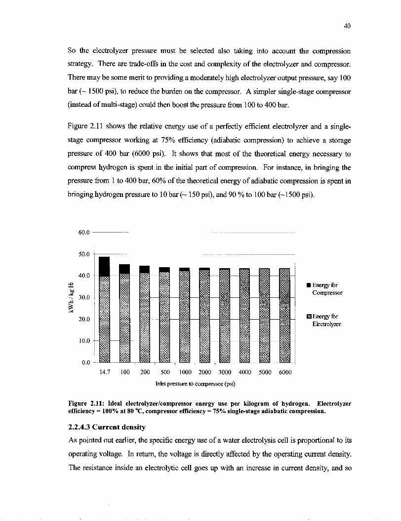
So the electrolyzer pressure must be selected also taking into account the compression
strategy. There are trade-offs in the cost and complexity of the electrolyzer and compressor.
There may be some merit to providing a moderately high electrolyzer output pressure, say 100
bar (- 1500 psi), to reduce the burden on the compressor. A simpler single-stage compressor
(instead of multi-stage) could then boost the pressure fiom 100 to 400 bar.
Figure 2.1 1 shows the relative energy use of a perfectly efficient electrolyzer and a single-
stage compressor working at 75% efficiency (adiabatic compression) to achieve a storage
pressure of 400 bar (6000 psi). It shows that most of the theoretical energy necessary to
compress hydrogen is spent in the initial part of compression. For instance, in bringing the
pressure fiom 1 to 400 bar, 60% of the theoretical energy of adiabatic compression is spent in
bringing hydrogen pressure to 10 bar (- 150 psi), and 90 % to 100 bar (-1 500 psi).
Energy fbr Compressor
Energy fbr Electrolyer
14.7 100 200 500 1000 2000 3000 4000 5000 6000
Inlet pressure to compressor (psi)
Figure 2.11: Ideal electrolyzer/compressor energy use per kilogram of hydrogen. Electrolyzer efficiency = 100% at 80 O C , compressor efficiency = 75% single-stage adiabatic compression.
2.2.4.3 Current density
As pointed out earlier, the specific energy use of a water electrolysis cell is proportional to its
operating voltage. In return, the voltage is directly affected by the operating current density.
The resistance inside an electrolytic cell goes up with an increase in current density, and so

does the operating voltage. Hence, the operating voltage and specific energy use of an
electrolysis cell are, to some extent, proportional to its operating current density.
The rate at which the operating voltage increases as a function of operating current density
depends on the particular electrolysis technology and cell design considered. For example, the
operating voltage in conventional AWE increases much more steeply with current density
than it does in SPE. That explains why conventional AWE operates at a fiaction of the current
density used in SPE (typically 0.2-0.5 A/cm2 for AWE vs. 1-3 A/cm2 for SPE). Therefore,
even though AWE requires less expensive cell materials, it needs about 3 to 5 times more
electrode surface area than SPE, as shown in figure 2.12. See references [5 1-52] respectively
for specific characterization of SPE and AWE current density vs. voltage relationships.
Current density (Alcrn2)
Figure 2.12: Relative electrode surface area as a function of current density.
For each design and application, there is an optimum current density that minimizes the
overall cost of hydrogen. This is shown clearly in a sensitivity analysis for SPE performed
within the Japanese WE-NET program [ 5 11, where they found the most cost-effective current
density to be in the range of 2-2.5 A/cm2.
Because the effect of current density varies widely between various electrolysis technologies,
it has not been included as a variable in the cost model developed for thls thesis. Instead, the
nominal rated operating current density is assumed in the specific capital cost of an
electrolyzer. However, other studies focusing on a single electrolysis technology (e.g.
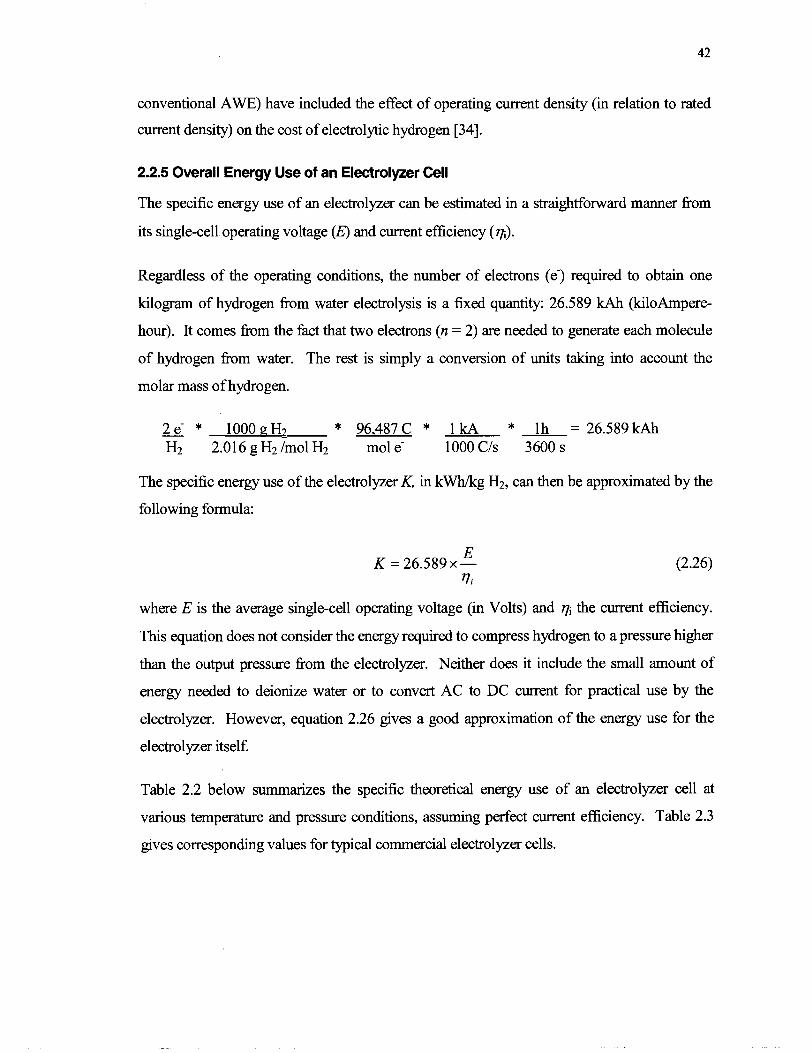
conventional AWE) have included the effect of operating current density (in relation to rated
current density) on the cost of electrolytic hydrogen [34].
2.2.5 Overall Energy Use of an Electrolyzer Cell
The specific energy use of an electrolyzer can be estimated in a straightforward manner fiom
its single-cell operating voltage (0 and current efficiency (q).
Regardless of the operating conditions, the number of electrons (e-) required to obtain one
kilogram of hydrogen fiom water electrolysis is a fixed quantity: 26.589 kAh (kilohnpere-
hour). It comes fiom the fact that two electrons (n = 2) are needed to generate each molecule
of hydrogen fiom water. The rest is simply a conversion of units taking into account the
molar mass of hydrogen.
2e- * 1000gH2 - * 96,487 C * 1 kA * lh = 26.589 kAh H2 2 . 0 1 6 ~ ~ 2 ? m 0 1 ~ 2 mol e- 1000 CIS 3600 s
The specific energy use of the electrolyzer K, in kWhkg H2, can then be approximated by the
following formula:
rli
where E is the average single-cell operating voltage (in Volts) and qi the current efficiency.
This equation does not consider the energy required to compress hydrogen to a pressure higher
than the output pressure from the electrolyzer. Neither does it include the small amount of
energy needed to deionize water or to convert AC to DC current for practical use by the
electrolyzer. However, equation 2.26 gives a good approximation of the energy use for the
electrolyzer itself
Table 2.2 below summarizes the specific theoretical energy use of an electrolyzer cell at
various temperature and pressure conditions, assuming perfect current efficiency. Table 2.3
gives corresponding values for typical commercial electrolyzer cells.
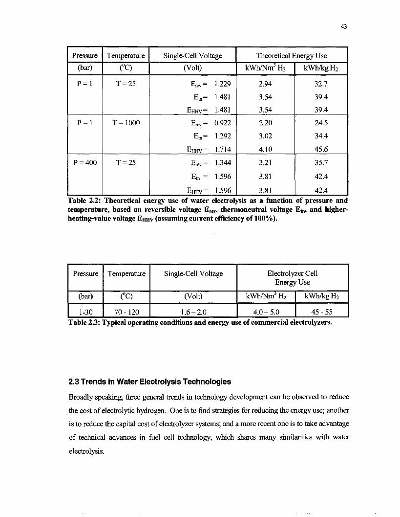
Table 2.2:
ergy Use
Em= 1.596 1 3.81 rheoretical energy use of water electrolysis as a function of pressure an1 -. -
temperature, based on reversible voltage Ere, thermoneutral voltage Eb, and higher- heating-value voltage EHHV (assuming current efficiency of 100%).
Table 2.3: Typical operating conditions and energy use of commercial electrolyzers.
2.3 Trends in Water Electrolysis Technologies
Broadly speaking, three general trends in technology development can be observed to reduce
the cost of electrolytic hydrogen. One is to find strategies for reducing the energy use; another
is to reduce the capital cost of electrolyzer systems; and a more recent one is to take advantage
of technical advances in fuel cell technology, which shares many similarities with water
electrolysis.

2.3.1 Decrease Energy Use
As explained earlier, the energy use is directly proportional to the operating voltage. One way
to keep ths voltage as low as possible is to lower the electrical resistance in the electrolyzer
hardware; namely by reducing the gap between electrodes to a minimum. Advanced
technologies use a "zero-gap" sandwich-type configuration, in which porous electrodes are
pressed on the opposite faces of the separatorlmembrane, and the gases evolve predominantly
on the backsides of the electrodes. Variations of this principle are applied to AWE, SPE and
HTE to reduce the electrical resistance [6 11.
Another approach is proposed to minimize the increased electrical resistance due to the
collection of bubbles at the electrodes at high current density. It consists of subjecting the
electrolysis cell to a centrifugal force to promote the mass transport within the cell and the
separation of gas bubbles fiom the electrodes, electrolyte and membrane. Experimental work
to test the validity of this approach was carried out by Cheng et al. on AWE cells in centrifugal
fields of up to 190 G [62]. The results were conclusive in showing a net reduction in energy
use for a given current density.
High temperhture electrolysis is another way to decrease the cost of energy by substituting
inexpensive heat instead of electricity. The German "HOT ELLY" electrolyzer developed at
the end of the 1980's and thin film electrolyzer cells developed at the Lawrence Livermore
National Laboratory (LLNL) are good examples of HTE [63]. HTE typically exhibits high
energy and current efficiencies compared to conventional AWE.
A more recent approach to cut drastically the operating voltage has been proposed and
demonstrated at LLNL. The principle is to supply natural gas on the anode side to reduce the
chemical potential difference across the electrolyzer, thus minimizing the electrical
consumption. The technique is an extension of HTE, taking place at 900 OC, and is called
natural gas assisted steam electrolysis (NGASE) [63]. Here, the oxygen produced from water
electrolysis is used to partially oxidize natural gas to CO and hydrogen (reactions 2.27 and
2.28). CO can be subsequently shfied to yield extra hydrogen (reaction 2.29). The
electrolysis voltage is then reduced close to zero since most of the energy comes from natural
gas (see figure 2.13).

With NGASE, when all the energy comes fiom natural gas instead of electricity, the overall
reaction is equivalent to the steam reforming of natural gas.
Cathode: H 2 0 + 2e- a H , + 02- (2.27)
Anode: CH, + 0*- 3 CO + 2H2 + 2e- (2.28)
Shift Reaction: C O + H 2 0 a H 2 + C 0 2 (2.29)
Overall reaction: CH, + 2H2 0 s 4H2 + CO,
In this case, the main advantage of NGASE is essentially a compact modular design for the
production of hydrogen fiom natural gas and water.
Figure 2.13: Current-voltage plots of conventional HTE and NGASE. Cathode inlet gas: HZ (3%) + HzO (70%) + Nz (balance). Anode inlet gas: CH4 (97%) + Hz0 (3%). [63]
High-pressure electrolysis could also help reduce the energy use, but only to a limited extent
as suggested by figure 2.11. The net result on energy use is arguable, as several effects are
compounded. For instance, high-pressure electrolysis decreases the ohmic resistance in the
electrolyhc cells and allows a more energy efficient isothermal compression of hydrogen; on
the other hand, larger parasitic currents are to be expected as a result of the reduced ohmic
resistance and thus lower current efficiency [54,64].

2.3.2 Reduce Capital Cost
Capital cost reductions can be achieved through clever engineering, cheaper materials or
economies of scale from mass production. Leaving aside the impact of mass production, the
main issues being worked on to reduce the capital cost of electrolyzers are summarized below.
For AWE technology:
Development of an alternative separator suitable for hgh-temperature operation to
replace the asbestos-based material used in conventional technology.
Development of inexpensive, more active and stable electrocatalysts.
0 Development of inexpensive construction and sealant materials resistant to alkaline
corrosion, particularly at higher temperature.
For SPE technology:
Reduction of platinum catalyst loading and development of non-noble metal catalysts.
Development of inexpensive electrolyte membrane materials, with adequate durability
and resistance to higher temperature and pressure.
Development of suitable fabrication techniques for the commercial production of
membrane electrode assemblies (MEA) and flow-field plates (current collectors).
For HTE technology:
Development of inexpensive ceramic electrolyte and catalyst systems.
Design optimization and scale-up.
Development of suitable fabrication techniques.
For all technologies:
Increase the operating current density as much as possible to reduce the size and
capital cost of the electrolyzer (at a reasonable cost in efficiency losses).
Optimization of the integrated system including the electrolyzer and all the ancillary
equipment, such as heat exchangers, water deionization and gas purifiers.
Simplification and reduction of the number of components required for an electrolyzer
plant.

2.3.3 Synergy with Fuel Cell Developments
Because a water electrolyzer is essentially a fuel cell operating in reverse, water electrolysis
technology could benefit directly from advances in fuel cells. That is particularly true of SPE
and HTE, two promising electrolysis technologies that could take advantage of developments
in their fuel cell counterparts, respectively PEMFC and SOFC, given that the vast majority of
R&D efforts and investments in fuel cells are concentrated in these two types of l e l cells.
For example, the U.S. DOE in collaboration with industry partners launched in 2001 a
US$500 million programme to achieve "ultra-low-cost" SOFC with a cost goal of $400/kW,
within 10 years [65].
Fuel cell technology could help water electrolysis on the technical front (improved design,
inexpensive materials, increased efficiency) as much as on the economic one (adapted
fabrication techniques, mass production).
Some innovative designs are exploiting the synergy between l e l cells and electrolyzers to
integrate both functions. Regenerative fuel cell (RFC) systems are integrated systems that can
produce power and regenerate their reactants using stacks of electrochemical cells. RFC
systems may have separate stacks to llfill the role of he1 cell and electrolyzer, or a single
stack may perform both functions, in which case it is called a unitized regenerative fuel cell
(URFC) [66]. A team of researchers working on URFC systems (based on PEM technology)
at Lawrence Livermore National Laboratory (LLNL) highlights the fact that their reversibility
allows them to provide their own l e l , wherever electricity is available [54]. Another example
of RFC development is a low cost, high-efficiency system based on hgh-temperature SOFC
technology [67].
2.4 Summary of Electrolysis Technologies and Main Players
This section identifies some of the main players active today in the water electrolysis market,
and presents a summary table of the characteristics of the three main types of water
electrolysis technology discussed in this chapter: AWE, SPE and HTE.
Stuart Energy Systems (formerly the Electrolyser Corporation) is a Canadian company with
over 50 years of experience in AWE. The company has delivered thousands of installations
around the globe and has provided electrolyzer lelling stations for demonstration projects of

hydrogen-fuelled FCVs, namely for fuel cell bus demonstrations in Vancouver and in
California. Stuart has developed a proprietary double electrolysis plate (DEP) technology that
increases the efficiency of the electrolysis equipment while lowering the capital cost. The
company became public in 2000 aRer raising CAN$1 SO million. In addition to the existing
industrial gas market and eventual hydrogen fuelling market, a major portion of revenues for
the company is expected to come fiom backup power applications. The company plans the
delivery of up to CAN$600 million worth of hydrogen-powered backup power units by 2008
to a single Asian client company. In 2003, Stuart acquired one of its competitors,
Vandenborre Technologies, which had developed the inorganic membrane electrolysis (ME)
technology [68].
In Europe, Norsk Hydro Electrolysers offers a range of electrolyzers based on AWE
technology, fiom atmospheric to high-pressure electrolyzers (15 bar), as well as hydrogen
fbelling stations. Norsk Hydro provided several hydrogen fbelling stations in Europe, namely
for fuel cell buses in Iceland [7]. MTU in Germany is also active in AWE and has developed
a high-pressure electrolyzer (30 bar in a pressurized container) together with Norsk Hydro
[69]. Forschungszentrum Jiilich, a German institute, has pursued the same approach pushing
the operating pressure up to 120 bar [64].
In SPE technology, Hamilton Sundstrand - a business unit of United Technologies Company
(UTC) - has been designing and manufacturing SPE electrolyzers for over 40 years. The
technology was first developed for space applications. Some SPE electrolyzers operating at
pressures of up to 3,000 psi (200 bar) have been qualified for use on board U.S. submarines.
With over 40 million hours of system operation, the maturity of their SPE technology is well
established. In 2002, the company entered into an alliance with Stuart Energy Systems to
jointly develop and market integrated hydrogen generation products (based on Hamilton
Sundstrand SPE technology) for vehicles, power generation and industrial uses [70].
Other companies involved in the development and commercialization of SPE electrolyzers
include Proton Energy Systems in the United States [71], Hydrogenics in Canada [72] and
Fuji Electric in Japan [50]. Proton Energy Systems and Hydrogenics are developing
electrolyzer products specifically targeting the hydrogen fuelling application. Hydrogenics
stresses that the modular and compact design of their fuelling stations allows them to be scaled
for increased hydrogen generation and storage requirements.
Finally, Lawrence Livermore National Laboratory (LLNL) 1631 and the small company
Technology Management Inc., both in the United States, are among the few working on HTE
technology.
Table 2.4 summarizes the characteristics and performance of the three main types of water
electrolysis technology discussed in this chapter: AWE, SPE and HTE. This table is adapted
from a paper published by Dutta [61], but some values were updated to reflect more recent
information available.

AW
E
SPE
Sol
id p
olym
er
elec
trol
vser
P
roto
type
s an
d co
mm
erci
al u
nits
1.
4-2.
0
HT
E
CI T
echn
olog
y :o
nven
tiona
l al
kalin
r el
ectr
olvs
er
Com
mer
cial
larg
e sc
ale
unit
s 1.
8-2.
2
Adv
ance
d al
kali
ne
elec
trol
vser
P
roto
type
s and
co
mm
erci
al u
nits
1.
5-2.
5
Inor
gani
c m
embr
ane
alka
line
ele
ctro
lvse
r C
omm
erci
al u
nits
Hig
h te
mpe
ratu
re (w
ate
va~
or)
elec
trol
vser
L
abor
ator
y-sc
ale a
nd
Dro
totw
e un
its
0.95
-1.3
7 w
pm
en
t st
age
m
Am
bien
t 1-
2 at
m
Up
to 1
20 a
tm
Up
to 4
0 at
m
Up
to 4
00 a
tm
Up
to 3
0 at
m
Ste
el, s
tain
less
stee
l or
nic
kel
Nic
kel
Cat
alyt
ical
ly o
r non
ca
taly
tica
lly
activ
ated
Ni
Cat
alyt
ical
ly o
r non
ca
taly
tica
lly
acti
vate
d N
i
Asb
esto
s-ba
sed
belo
w
1 OO
•‹C; T
eflo
n-bo
nded
po
lybe
nzim
idaz
ole
(PB
I)
K-t
itan
ate
abov
e 10
0•‹C
0.
5-0.
7 SZ
cm
-2
25-4
0% K
OH
NiS
C
arbo
n fi
ber p
aper
& a
laye
r of
Pt c
atal
yst
Poro
us ti
tani
um w
ith
a la
yer
of a
pro
prie
tary
r.ntnlvnt
Mul
tila
yer e
xpan
ded
met
al s
cree
ns
Spi
nel o
xide
bas
ed o
n C
o N
i-N
iO o
r P
erov
skit
e (L
aNi0
3, L
aMn0
3, et
c)
Non
e Pa
tent
ed p
olya
ntim
onic
ac
id (
PAM
) mem
bran
e 0.
2-0.
3 SZ
cm
-2
Asb
esto
s 1.
2-1.
7 SZ
cm-2
25-3
5% K
OH
14
-15%
KO
H
Per
fluo
rosu
lfon
ic ac
i<
mem
bran
e 10
- 12
mil
s 0 4
6 .O
. cm
-'
85-9
8%
Solid
Y20
3-st
abil
ized
Z
a380
E
lect
roly
te
sa
ower
con
sum
ptio
n
Stu
art
Nor
sk H
ydro
S
tuar
t Ji
ilich
N
orsk
Hyd
ro
Tel
edyn
e
Stu
art &
V
ande
nbor
re
Tec
hnol
ogie
s
Stu
art &
H
amilt
on S
unst
rand
P
roto
n E
nerg
y H
ydro
geni
cs
Fuj
i
LL
NL
'e
thno
logy
Man
agem
en
Inc.
(T
MI)
laye
rs I

Chapter 3 - Cost Model 3.1 General Considerations
In line with the objectives of this research, an original cost model was developed to integrate
and investigate the technical, economic and comparative aspects of decentralized electrolysis.
This model builds on previous studies and includes a monetary valuation of GHG emissions,
site-specific information, and a more detailed account of the theoretical energy requirements.
Considering that the model's main challenge lies more in the number of variables to be
connected than the mathematical complexity of its equations, the software MS Excel 2000
was deemed to be an appropriate platform, and selected on the basis of its simplicity and wide
use.
Previous similar cost models for electrolytic hydrogen have inspired the structure of the core
aspects. The primary reference source used is a 1995 report written by Thomas and Kuhn
(DTI) for the National Renewable Energy Laboratory (NREL), a national laboratory of the
U.S. Department of Energy (DOE) [43]. Other significant references used are a report fiom
The Electrolyser Corporation (now Stuart Energy Systems) prepared for the Ford Motor
Company [42], as well as published work by J. M. Ogden (Princeton University) [29,40] and
Dutta et al. (Florida Solar Energy Centre) [55]. For the portion dealing with GHG emissions,
the results fiom a 2000 report by the Pembina Institute [5] and a paper by Dones et al. (Paul
Scherrer Institute) [73] constitute the principal sources. Additional references used to support
these sources are other published work by Thomas et al. [4] and a study done by the
International Atomic Energy Agency (IAEA) [74].
In developing the model, more emphasis was placed on enswing proper sensitivity to the
various input parameters than selecting the most representative values for the base case.
Nevertheless, in order to preserve the desired level of flexibility, some actual couplings
between variables are not reflected in the model. For instance, the specific capital cost of the
electrolyzer ($/kWe), whch is an input parameter in the present model, would be affected in
reality by the operating current density, the resulting energy efficiency and the number of
electrolyzers manufactured, couplings that are not explicitly defined in the model. The
empirical relationships between these variables vary depending on the technology used and

the sources consulted. Therefore, special care in reviewing the assumptions should be
exercised before entering a given set of input values, and equal caution should be use used in
interpreting the results.
3.2 Description of the Model
The cost model developed has one primary output variable: the unit cost of electrolytic
hydrogen delivered to the consumer, U, in US$ per lulogram. This variable is used to study
the economics of electrolytic hydrogen for FCVs fiom both an "absolute" and a
"comparative" standpoint. The former is concerned with the sensitivity of U itself to a
number of technical and economic parameters incorporated in the model. The latter compares
the price of electrolytic hydrogen to that of other fuelling options, based on inputs for both
electrolytic hydrogen and the other fuelling options.
The comparative portion includes the possibility to assess the economic impact of GHG
emissions on the price of electrolytic hydrogen, with respect to other fuelling options. This is
done by assignmg a fixed monetary value to these emissions ($/ton of C02-equivalent), which
vary depending on the fuel option considered, and as a function of the electricity mix in the
case of electrolytic hydrogen.
The specific cost of hydrogen, U, is simply obtained fiom the following ratio:
where U = specific cost of electrolytic hydrogen ($/kg)
C = annual cost to produce electrolybc hydrogen ( $ 1 ~ )
Y = annual hydrogen production fiom dispensing station (kglyr)
The annual cost to produce electrolytic hydrogen, C, is defined as:
C = c, + C,(+C,,,)
where C, = capital, operating and maintenance cost ($/yr)
C, = annual energy cost ( $ 1 ~ )
CGHG = relative additional costhaving related to GHG emissions ($/yr)
C, and C, are always positive values, as they correspond to real costs associated with the two
principal economic components of water electrolysis, i.e. capital and energy costs.
Consequently, they are always included in the calculation of C.
On the other hand, CGHG is treated as a relative term whose value can be either positive (in the
case of hgher GHG emissions than the alternative fbelling option considered) or negative (i.e.
a credit, in the case of lower GHG emissions than the alternative fbelling option considered).
The value of CGHG depends on several inputs for both the electrolytic hydrogen and alternative
fuelling option to which electrolyhc hydrogen is compared. As a result, CGHG is not a real cost
or saving, but rather an indicator of the economic advantage of electrolyhc hydrogen related to
GHG emissions reduction. The model allows CGm to be included or omitted in the
calculation of C, as reflected by the parentheses in equation 3.2. Although somewhat
artificial, h s component of the hydrogen cost offers a guideline for the relative impact of
policy based on the economic evaluation of GHG emissions.
The annual hydrogen production, Y, is determined by the fbelling needs of the vehicles served
by the electrolytic hydrogen dispensing station.
where V = number of vehicles served by the fbelling station
M = average annual mileage of a vehicle (krnlyr)
& = average he1 economy (km/kg H2)
The fuel economy,&, in kilometres per kilogram of hydrogen, can be estimated either directly
ffom published data or by converting the energy requirements of a typical FCV, expressed in
terms of equivalent gasoline fuel economy. Most published studies [4,5,40] express the fuel
economy of direct hydrogen FCVs in terms of equivalent gasoline fuel economy, as people
are generally familiar with this measure. Some studies use the higher heating value (HHV) of
the fuels as a basis for equivalence [40], some use the lower heating value (LHV) [4], and
others don't specify whch one is used [ 5 ] . The main argument for LHV comes ffom the fact
that ICE efficiency is traditionally expressed in reference to the LHV energy content of the
hel. The counter argument for HHV is that this value reflects more accurately the true energy

content of a fuel. For consistence in this research, the HHV-basis is always the one used when
expressing an equivalent gasoline &el economy for hydrogen or methanol. See Appendix B
for &el economy conversion. Figure 3.1 below presents a schematic of the model's structure.
4 Fuel Comparison
4 t I Site-specific Information I
Figure 3.1: General structure of the cost model.
3.2.1 C,: Capital and Operating Cost
Essentially, the capital and operating cost component considers all the expenses that are
associated with the electrolytic hydrogen station, with the exception of the energy cost. It
includes the ,initial installed capital cost, maintenance, major parts replacement, insurance,
property taxes, etc. It also takes into consideration economic parameters, such as the expected
rate of return on capital investment.
The annual capital and operating cost, C,, is expressed as a fi-action of the electrolyk
hydrogen dispensing station's total installed capital cost, C,,. If extraordinary expenses occur
at later points, they are distributed over the lifetime of the station to reflect their impact on the
annual capital and operating cost, C,.

where Ccap =
cRF=
C, = Ccap (CRF, + op + ins + t ) + CRF [ j (::;in) total installed capital cost of H2 dispensing station: electrolyzer, compressor,
hydrogen storage and associated balance of plant
capital recovery factor
CRF, = effective capital recovery factor
op = operating and maintenance costs (% of Ccap)
ins = annual insurance (% of C,,, )
t = annual property taxes (% of Ccap)
Ei = ih extraordinary expense on nh year ($)
d = discount rate (%)
The model allows four distinct capital costs to be included in Ccap: electrolyzer, e, compressor,
c, hydrogen storage, s, and a miscellaneous one called balance of plant, x. In the scenarios
used for sensitivity analysis, only the first three categories are assigned a value, whereas
related equipment is combined with either one of them. For example, the hydrogen
dispensing equipment cost is included in the compressor portion and the power systems and
controls' cost is incorporated in the electrolyzer portion. However, the balance of plant
component, x, allows for more flexibility when there is a need to treat some peripheral
components separately.
Ccap is therefore defined as:
Ccap = ( e + c + s + x )
where e = capital cost of electrolyzer ($)
c = capital cost of compressor ($)
s = capital cost of storage ($)
x = capital cost of balance of plant ($)
Each of these capital cost components depends on the size of the electrolyzer station, which is
in turn largely determined by the number of vehicles to be served. The maximum required
hydrogen production flow in ~ m ~ / h , QH2-, is obtained from:

where Y = annual hydrogen production fi-om dispensing station (kdyr)
Rpd = ratio of peak hydrogen production to average demand
f = capacity factor
The numerical values are merely for conversion fi-om annual to hourly production rate, and
fi-om kilogram to normal cubic meter ( ~ m ~ ) of hydrogen.
In addition to the expected average hydrogen demand fi-om FCVs, the electrolyzer station
must be able to handle various fluctuations in demand due to statistical surges, as well as
daily, weekday-weekend and seasonal variations. These fluctuations must be accommodated
by some combination of hydrogen storage and load following by the electrolyzer system. The
ratio of peak hydrogen production to average demand, Rpd, accounts for the load following
portion. If for instance Rpd = 1.2, it means the electrolyzer's nominal production capacity is
sized 20% higher than the expected average demand. Moreover, it is assumed that any
electrolyzer can operate at production rates above this nominal output for short periods of
time, although possibly at lower efficiency [43].
The capacity factor,x essentially accounts for the fact that the electrolyzer typically would be
operated less than 24 hours a day to take advantage of lower electricity rates, which affects
directly the size of the electrolyzer. For example, an electrolyzer operating 12 hours a day on
off-peak electricity rates would have a capacity factor of 0.5, and would therefore be sized for
about twice the production rate of an equivalent electrolyzer operating around the clock.
The maximum hydrogen production rate can also be expressed in terms of the energy content
(HHV value) of the hydrogen produced, k,,, in kilowatt (kW).
k,,, = 3.5418 *QH2,,
The conversion factor between em,, and k,,, comes fi-om:
l & ~ ~ = l N m ~ ~ ? * 1 kaH? * 141,860k.T (HHV) * lh - 3.5418 kW (HHV) h h 11.126 Nm3 H~ kg H2 3,600 s

Figure 3.2 presents the variables and simplified equations affecting the four components of the
electrolyzer station capital cost C,,,. The first line in each sub-box indicates what variables or
quantity determine the value of the capital cost component.
The electrolyzer capital cost, e, is determined by the required maximum hydrogen production
rate, kOut, the electrolyzer useful efficiency, qu, and the estimated specific capital cost per kW,
at nominal production, e, (equation 3.9). The so-called electrolyzer useful efficiency is
actually calculated automatically in the model (equation 3.8) and is defined as the following
ratio:
Heating value of H7 output (HHV) @ 25 "C [in k m g H2] Energy input: elect&ty + NG (HHV) [in kWhikg H2]
The heating value (HHV) of hydrogen at 25 OC is a fixed value of 39.4 kWkg H2 [48]. The
energy input to the electrolyzer is nearly always limited to electricity, however natural gas has
been added as a possible energy input to investigate the potential effects of natural gas assisted
steam electrolysis (NGASE - see Chapter 2). The energy input is calculated fiom the
theoretical energy requirement for water electrolysis at a given temperature, kelfh (in kwkg)
divided by the energy efficiency of the electrolyzer, qe. The main difference between 77, and
rl, is that the latter does not consider any of the additional heat contained in the output
hydrogen gas (at the electrolysis reaction temperature) to be usable, resulting in a slightly
lower value for q, than qe; a dif fmce that grows as the temperature of electrolysis is
increased.
39.4 rl, =- [!$I
Assuming that hydrogen is stored onboard FCVs as a compressed gas, a compressor system is
necessary to bring hydrogen to the desired high-pressure level. The compressor capital cost, c,
depends on the required maximum hydrogen production rate, kout, and the estimated specific
capital cost of the compressor system per kWM at nominal production, cu (equation 3.1 0).

e, = unit cost of electrolyzer ($/kW,)
Y = Annual H2 production (kg!yr)
D = Equivalent number of days of
A = Available •’faction of stored H2
c, = unit cost of compressor
x (specified in each individual case - if needs to be treated separately)
Figure 3.2: Components included in the electrolyzer station capital cost C,,,.
It is assumed that storage tanks would be required to accommodate both the intermittent
nature of the electrolytic hydrogen production and irregular load profiles. The hydrogen
storage capital cost, s, is determined by the maximum storage capacity requirement for the
reheling station and the estimated specific capital cost of the storage tanks, s,.
The storage capacity should cover at least the average daily production of hydrogen, which is
likely to be consumed at a different time of the day than it is produced, i.e. off-peak electricity
hours. In addition, DTI [43] recommends the equivalent of another 111 day average
production for unexpected equipment failures and surges in demand. The storage capacity can

therefore be expressed in "equivalent number of days of storage", D, at the average production
rate (equation 3.1 1). For example, a 2-day storage capacity (D = 2) would accommodate a full
day's shutdown of the electrolyzer for repairs and maintenance. Also, not all of the hydrogen
stored in high-pressure vessels is available, because some of it will remain in the storage tanks
as the pressure falls during transfer to the vehicle tanks. DTI quotes an industrial gas company
saying that even with multiple tanks and cascade filling, at best 60% of the stored hydrogen
can be utilized [43]. The "available fiaction of stored hydrogen", A, accounts for this
limitation (equation 3.1 1).
Although the full installed capital cost C,, may have to be spent initially, only a fiaction of it
needs to be recovered annually. Thls fiaction is called the effective capital recovery factor,
CRF,, which can be determined fkom the financing parameters. Other more or less fixed
annual costs, such as operating and maintenance, op, insurance, ins, and property taxes, t, may
also be expressed in terms of the installed capital cost Ccap. The sum of these four fiactions
constitutes thk multiplying factor for Ccap presented in equation 3.4. Figure 3.3 presents the
variables and equations used to calculate the effective capital recovery factor CRF,, along with
the other three components of the multiplying factor.
The capital recovery factor, CRF, is a function of the discount rate, d, and economic recovery
period, N, as given by equation 3.12. DTI [43] proposes two different scenarios to calculate
the discount rate: one where individual consumers can finance small "electrolyzer fuelling
appliances" as part of their home mortgage, and a business case where the electrolyzer station
is financed by a company just like any other investment with a given expected after-tax rate of
return (corrected for inflation). Equations 3.1 3 and 3.1 5 respectively show how the discount
rate, d, is calculated for each of these two options. For the home mortgage case, d is equal to
the mortgage interest rate corrected for the fact that interest payments are considered to be
deductible fiom income tax. For the business case, d is equal to the after-tax real rate of
return, r (corrected for inflation).

Capital Recovery Factor
CRF = f (d, N)
d = discount rate N = recovery period in years
CRF = d
1 - ( 1 + d ) - ~ To calculate the discount rate d: i, = mortgage interest rate T, = personal tax rate of home owner i = general inflation rate r = after-tax real rate of return on investment Tb = business tax rate
Home mortgage case Business case d = i , * ( I -T , ) (3.13) d = r + i ( l+ r ) (3.15)
Effective Capital Recovery Factor
CRF, = CRF
Figure 3.3: Components of the annual multiplying factor for C,,,.
The "effective capital recovery factor" CRF,, was artificially created to lead to the more
general form of equation 3.4 for the annual capital and O&M cost. CRF, is identical to CRF
for the home mortgage case. For the business case however, CRF, needs to account for the
corporate income tax rate, Tb, which requires the selection of a depreciation schedule. Both
DTI and Electrolyser Corporation [43, 421 use straight-line depreciation on the basis of its

simplicity, stating that it gives close enough values to the Modifid Accelerated Cost
Recovery System (MACRS) specified by the American Internal Revenue Service. So this
model also adopted the straight-line depreciation schedule, leading to equation 3.16, in
accordance with what is specified in engineering economics textbooks [75] for this
depreciation schedule.
DTI also considers a third scenario in addition to the home mortgage case and the business
case: that of a utility financing the electrolyzer station. This case is treated just like the
business case, but with a tax rate Tb equal to zero [43].
The other three costs that are part of the multiplying factor in figure 3.3: operating and
maintenance, op, insurance, s, and property taxes, t, are calculated independently and
expressed simply as a percentage of the installed capital cost C,,.
One expense which is not considered explicitly in the present model, and which could be
added to the operation cost op, is the cost of tap water utilized to produce hydrogen &om
electrolysis. Based on a requirement of approximately 13 litres of water per kilogram of
hydrogen [42], and a water price of $1.00/m3 in Los Angeles [29], this translates in a cost of
water of $0.013/kg HZ, or in the order of 0.5% of the base case hydrogen price. The average
hydrogen requirement for a FCV would necessitate about 7 litres of water per day, i.e. less
than a typical toilet flush, or a &action of current daily water use in industrialized countries
(350 litres per person p a day in Canada [76]).
Extraordinary expenses (such as catalyst replacement every five years) are calculated in the
same way they are treated in the Electrolyser report [42]. The present worth of an
extraordinary expense Ei occurring in year ni is given by:
This cost must be amortized over the N years of the economic recovery period by the capital
recovery factor CRF. Hence, the calculated annual cost of an extraordinary expense Ej
occurring in year ni is equal to:

CRF * Ei (ni ) (1 + d y i
The sum of these extraordinary expenses makes up the last term of equation 3.4, completing
the general elements considered in the annual capital and operating cost C, of an electrolyzer
rebelling station.
3.2.2 C,: Energy Cost
There are two main reasons to treat the cost of energy separately from the capital and O&M
costs in the model. 1) It is a variable cost, nearly proportional to the quantity of hydrogen
produced, whereas capital and O&M costs are essentially fixed expenses. 2) The cost of
electricity is often the dominant component of electrolyhc hydrogen's total cost, typically
between 50% and 80 % [40,43,55].
The simplified process diagram below (figure 3.4) shows the various material and energy
inputs and outputs fiom an electrolytic hydrogen station, with the energy consuming items
listed in the central box.
Electrolyzer
Water electrolysis Power conversion (ACJDC) Conditioning of water input Compressor
Controls & Safety
L
I I I I
v Waste Heat
Pressurized H?
( C 0 2 and trace emissions) - - - - - - b
Figure 3.4: Simplified process diagram for electrolytic hydrogen dispensing station
The bold arrows represent material and energy flows that are accounted for in the cost model.
Conventionally, the energy required for an electrolytic hydrogen dispensing station is
provided in the form of electricity exclusively. However, there is also the possibility in a
decentralized scenario to use natural gas for providing a portion of the necessary heat and/or
contributing to the electrolysis reaction (NGASE - Natural Gas Assisted Steam Electrolysis).
Accordingly, the energy currencies considered as possible inputs for the dispensing station
include electt'icity (e') and natural gas (NG).
The energy cost for the electrolyzer includes the electrolysis reaction itself, water conditioning
(to bring feed water to electrolysis operating temperature), and ACDC conversion to provide
DC current to the electrolyzer. The input variable for the electrolyzer energy efficiency, 77,
(defined later), must account for the combined inefficiencies of both the electrolysis reaction
and the ACIDC conversion. For water conditioning, the conservative assumption made in the
model is that none of the waste heat fiom the electrolyzer is used to bring the feed water to
electrolysis temperature.
Another conservative assumption is made for the energy cost of the compressor, considering
that all of the hydrogen produced needs to be compressed to the nominal storage pressure (e.g.
414 bar or 6,000 psi). In reality, the necessary output pressure fiom the compressor will
increase progressively as each storage tank is filled to nominal storage pressure, in a multiple-
tank cascade filling arrangement. Finally, the electricity cost for controls is considered
negligible in proportion to the electrolyzer and compressor and therefore omitted in the model.
The flows represented by dotted arrows in figure 3.4 do not affect the energy cost in the
model. Feed water is assumed to be at room temperature (25 "C) when it enters the system.
No waste heat fiom the system is considered to be recycled. No energy (chemical or thermal)
fiom the oxygen out flow is considered to be recycled. Oxygen is simply assumed to be
vented out.
In the end, the total annual energy cost of the electrolytic hydrogen dispensing station, Ce, can
thus be approximated as the sum of the energy costs for the electrolyzer and compressor.
where Cel = annual cost of energy for electrolyzer ($/yr)
Ccomp = annual cost of energy for compressor ($/yr)
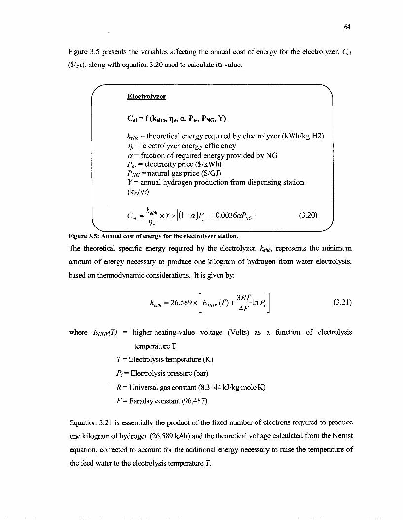
64
Figure 3.5 presents the variables affecting the annual cost of energy for the electrolyzer, CeI
($/yr), along with equation 3.20 used to calculate its value.
f Electrolvzer
kelth = theoretical energy required by electrolyzer (kWh1kg H2) ve = electrolyzer energy efficiency a = fraction of required energy provided by NG Pe- = electricity price ($/kwh) PNG = natural gas price ($/GJ) Y = annual hydrogen production from dispensing station (kg/Y-)
C,, = h x Y x [(1 -a)<- + 0.0036a~,,] rl,
Figure 3.5: Annual cost of energy for the electrolyzer station.
The theoretical specific energy required by the electrolyzer, kelrh, represents the minimum
amount of energy necessary to produce one kilogram of hydrogen from water electrolysis,
based on thermodynamic considerations. It is given by:
k,, = 26.589~ Em, (T) +-lne 4F 3RT I
where EH&) = higher-heating-value voltage (Volts) as a function of electrolysis
temperature T
T = Electrolysis temperature (K)
Pi = Electrolysis pressure (bar)
R = Universal gas constant (8.3 144 kJAqgmole-K)
F = Faraday constant (96,487)
Equation 3.21 is essentially the product of the fixed number of electrons required to produce
one kilogram of hydrogen (26.589 kAh) and the theoretical voltage calculated from the Nernst
equation, corrected to account for the additional energy necessary to raise the temperature of
the feed water to the electrolysis temperature T.

The higher-heating-value voltage E m (T) is obtained fiom an empirical relationship, based
on theoretical values (See Appendix A)
Recall from chapter 2 that for a given temperature, there are three distinct theoretical voltage
values for water electrolysis: the reversible voltage (AG/2F), the thermoneutral voltage
(AH/2F) and the so-called higher-heating-value voltage (Em); see figure 3.6. Em is always
the highest of them, including a portion that accounts for the electrolysis reaction itself and a
portion for bringing the feed water to electrolysis temperature.
Thermoneutral, Reversible and HHV Voltage
Temperature (K)
Figure 3.6: Theoretical electrolysis voltages as a function of temperature.
Although other sources consider the thennoneutral voltage (AW2F) as the theoretical
reference for calculating the energy efficiency of electrolysis, the present model selected Em
instead to include the energy required to bring the feed water to electrolysis temperature.
The theoretical specific energy required by the electrolyzer, kelth, can therefore be split in the
following two components:
kelth = ke! + khHZO
where ker = theoretical specific energy for electrolysis reaction (kWhikg H2)
k h ~ ~ ~ = theoretical specific energy to heat feed water (kWh/kg H2)
kel can be calculated fiom:
AH (T) is obtained fiom an empirical relationship, based on theoretical values (see Appendix
A). AH(T)/2F is the thermoneutral voltage for water electrolysis as a hc t ion of electrolysis
temperature. AH (T) is calculated for water in a liquid phase below 100 "C and in a gaseous
phase above 100 O C .
khHZo can be calculated fiom the difference between kelh and ker:
k,,, = 26.589 x EHH, (T) - - 2 F
Now, ker may also be divided in two components:
kel = kelAG + kelTAS (3 .25)
where keldG = specific change in Gibbs fkee energy to electrolyze water (kWhikg H2)
kelTdS = specific heat required for the electrolysis reaction (kWhlkg H2)
And each of these components may be calculated respectively fiom equations 3.26 and 3.27:
AG (T) is obtained fiom an empirical relationship, based on theoretical values (see Appendix
A). AG(T)/2F is the reversible voltage for water electrolysis as a hc t ion of electrolysis
temperature.

The electrolyzer energy efficiency, qe, which is an input variable to the model, is defined as:
Specific theoretical enerm required by electrolvzer (kelhl [in kWhkg Hz] Actual specific energy input: electricity + NG (HHV) [in k w g Hz]
Getting back to the annual energy cost for the electrolyzer, Ce17 once the actual specific energy
requirement (in kWhkg Hz, including both electric and thermal) is determined by kelth and G,
it is simply multiplied by the annual hydrogen production fiom the dispensing station Y, and
by the average price of energy ($/kWh). The 0.0036 factor in the last term of equation 3.20
simply reflects the conversion of the natural gas price fiom $/GJ (HHV) to $/kWh.
C,, = L x - Y x [(1 -a)<. + 0 . 0 0 3 6 a ~ , ] ' l e
In cases where natural gas is used as an energy input (in addition to electricity), this
approximation has the disadvantage of using a single efficiency value applied equally to both
electricity and natural gas.
Figure 3.7 presents the variables affecting the annual cost of energy for the compressor, C,,,
($/yr) along with equation 3.28 used to calculate its value.
Compression subsystem \ Ccomp = f (kcth, q c , Pe-9 Y) kcth = theoretical energy required for compression (kWhkg H2)
= compressor efficiency Pe- = electricity price ($/kwh) Y = annual hydrogen production from dispensing station (kglyr)
Figure 3.7: Annual cost of energy for the compressor subsystem

The theoretical specific energy for the compression of hydrogen, kcth, is defined as the energy
required for compressing one kilogram of hydrogen kom the electrolyzer pressure, Pi (also
considered to be the compressor's inlet pressure), to the maximum storage pressure, Po (also
considered to be the compressor's outlet pressure). In an actual compressor, the compressed
gas is heated, making adiabatic compression a better approximation than isothermal
compression [43]. The power required for adiabatic compression Padjab (in Watts) is given by:
where Mf = gas mass flow rate (molels)
R = gas constant (8.3 144 J1mol.K)
T = temperature (K)
Pi = inlet pressure to compressor
Po = outlet pressure
y = ratio of specific heats for the compressed gas
Since a flow rate of one kilogram of hydrogen per hour is equivalent to 0.1378 molls, it means
that equation 3.29 can be modified to give the theoretical specific energy for hydrogen
compression, kcth (in k m g H2) for 100% efficient adiabatic compression.
with the following assumptions used in the model:
T = temperature = 298 K
y = ratio of specific heats for hydrogen = 1.42
Compression is always evaluated at 298 K in the model, because temperature can otherwise
have a substantial effect on energy requirement for compression. Overall, the evaluation of
kcth for the model is considered to be a conservative approximation since it assumes all
hydrogen needs to be compressed to the maximum pressure, and the formula used is for
single-stage compression, typically less efficient than a more likely multi-stage compression.
This is counterbalanced to a lesser extent by the treatment of hydrogen as a perfect gas, which

is quite accurate for intermediate pressures, but underestimates the energy requirement for
compression by about 20% at 414 bar (6000 psi).
The annual cost of energy for the compressor, Ccomp, can then be calculated fiom equation
3.28 based on the value found for kcth, the compressor efficiency rl, (which is an input variable
in the model), the annual hydrogen production Y and the price of electricity Pe-.
Although not used directly in calculations, the model also gives the total specific energy use, K
(kWh/kg H2) including the electrolyzer and compressor portion:
l h s summarizes how the annual energy cost C, of the electrolyzer station is calculated in the
model fiom the electrolyzer and compressor energy requirements.
3.2.3 CGHG: Relative Cost or Saving Due to GHG Emission Evaluation
The motivation for including this component in the cost of hydrogen was to give an indication
of the potential impact, on the cost of electrolytic hydrogen, of policy relying on a monetary
valuation of C02 emissions.
Conventionally, this term would be treated as an absolute value added to the cost of all fuel
options, to account for the effect of a carbon tax applied on the basis of their respective GHG
emissions. However, this type of direct carbon tax would simply add further taxes to the
existing ones on gasoline and other hydrocarbon fuels, a scenario that could meet substantial
resistance fiom consumers. Arguably, a more likely scenario for the introduction of hydrogen
as a fuel is that lower GHG emissions would be reflected by some credits or lower taxes. The
important point for th~s research was to assess the magnitude of the relative advantage of
electrolyhc hydrogen versus other fuel options in terms of GHG evaluation, irrespective of
whether this is translated later in the form of taxes, credits or other fiscal incentives.
Consequently, it was decided to treat the value of CGm as a relative term that can be either
positive (in the case of higher GHG emissions than the alternative fbelling option considered)
or negative (i.e. a credit, in the case of lower GHG emissions than the alternative fuelling

option considered). Given its hypothetical value at this point in time, the model offers the
choice to include or ignore its effect on the unit cost of hydrogen, calculated from the other
two cost components: "capital and O&M" and "energy".
Figure 3.8 presents an example of output results fiom the cost model in Excel 2000. In the
upper portion, it shows the cost distribution for electrolyhc hydrogen excluding any influence
of GHG evaluation; in the lower portion it shows the effect of considering the relative GHG
costhaving in comparison with each of the alternative fuelling options.
Relative cost/saving due to GHG emissions evaluation
Assurnmg a GHG evaluat~on of: 1 20 UStlVtonne C& eq~b&@nt
Compared to: Added cost (positive) or saving (negative) b rn I
Gasoline FCV with on-board reforming
Figure 3.8: Example of output from the cost model, showing how the relative GHG costlsaving component cap be ignored or included for comparison with each of the alternative fuelling options.

Figure 3.9 presents the variables affecting the annual costkaving due to GHG evaluation,
CGHG ( $ 1 ~ ) along with equation 3.32 used to calculate its value. Note that since there are four
alternative fuelling options to which electrolytic hydrogen can be compared, CGHG can take on
more than one value, accounted for by the '3" subscript for each of these four alternatives.
The four fuelling options to which a direct-hydrogen FCV using electrolytic hydrogen can be
compared in the model are:
Gasoline internal combustion engine (ICE) vehicle
Gasoline FCV with on-board reforming
Methanol FCV with on-board reforming
Direct-hydrogen FCV with H2 fiom decentralized steam methane reforming (SMR)
Annual GHG cost or saving
altj = jth alternative fuelling option to which electrolytic hydrogen is compared (j = 1,2,3,4)
M = average annual mileage (kmlyear) V = number of vehicles served by the station
GHGelh = C02-equivalent emissions per kilometre from FCV using electrolytic hydrogen (g C02 qUiv/km)
~ f i ~ a z t j k , = C02-e uivalent emissions per kilometre from vehicle P using j alternative fuelling option (g C02 quiv/km) EC02 = monetary evaluation of C02-equivalent emissions
($/ton C02)
\ I Figure 3.9: Annual cost or saving associated with GHG emissions.
The general approach is to determine the difference in C02-equivalent emissions per kilometre
between electrolyhc hydrogen and the other fbelling options, and translate this difference into
an economic quantity based on the monetary value assigned to C02-equivalent emissions. In
the context of the model, this potential saving or additional cost per kilometre can be

multiplied by the number of vehicles served by the electrolyzer station and the average annual
mileage per vehicle to give the total annual GHG-related potential saving or additional cost,
CGW associated with the station versus each of the four other fuelling options considered.
In equation 3.32, only the C02-equivalent emissions per kilometre, respectively GHGelh for
electrolytic hydrogen and GHGaltjh for the alternative fuelling option, are not direct input
variables in the model. Here is how each of these two values is obtained.
First, GHGelh can be obtained fi-om the C02-equivalent emissions per kilogram of
electrolytic hydrogen, via the FCV he1 economy:
where GHGelkg = C02-equiv. emissions per kilogram of electrolytic H:! (g C02 ,&kg H2)
f, = average fuel economy (kmlkg H2)
Now, the value of GHGelkz is obtained from:
where C02kwhel = C02 emissions from electricity generation (g C02 ,h /kwh, delivered)
kelth = theoretical energy required by electrolyzer (kWh/kg H2)
qe = electrolyzer energy efficiency
kcth = theoretical energy required for compression ( k W g H2)
= compressor efficiency
a = fraction of required energy provided by NG
The value of C02kWhel is calculated automatically in the model fi-om the specified electricity
mix, based on representative figures for C02-equivalent emissions fi-om various energy
sources. The ones used are based on the Western Europe average [73] and in reasonable
agreement with similar figures from a different source at the International Atomic Energy
Agency (IAEA) [74].

The GHG emissions associated with each energy source used for power generation are
presented in table 3.1, along with an example of electricity mix and the corresponding
calculated C02-equivalent emissions. To determine the electricity mix, one simply has to
select a location (Vancouver, Los Angeles, Paris or "other location") and the electricity mix
entered in the site-specific worksheet for that location would be used for calculating C02kWhel.
Mix 1 source I GHG emissions ' I GHG emissions contribution
Table 3.1: Example of electricity mix and specific GHG values used in the model
Equation 3.34 gives the C02-equivalent emissions per kilogram of hydrogen by calculating
the portion coming fi-om electricity (electrolyzer and compressor) and the portion coming
fi-om natural gas, if applicable. The numerical value 178.3 in the second term actually stands
for 178.3 grams of C02-equivalent emissions per kwh (HHV) of natural gas. It comes fi-om
an estimate of C02 emissions by use natural gas, approximating natural gas as methane (CH4)
and considering that 100% of it is transformed into C02.
1 P CHa__ * 3600 s * 44 n C02 = 178.3 n COa q~, 55.5 kJ (HHv) h 1 6 g C b kwh NG (HHV)
These are optimistic assumptions, good enough for the purpose of this model, but which tend
to minimize the actual C02-equivalent emissions from natural gas. Also, as pointed out
earlier, equation 3.34 has the disadvantage of utilizing the same electrolyzer energy efficiency
figure for both the electricity and NG portions, minimizing again in most cases C02 emissions
from NG.
The C02-equivalent emissions per kilometre for the "j"' alternative fuelling option,
GHGaltjh, are adjusted in reference to base case values of C02-equivalent emissions per
kilometre and corresponding fuel economy for each of the four fuelling options considered.
Laltj GHGaltj, = - * GHGaltj,,
Laltj,,
where GHGaltjk, = C02-equivalent emissions per kilometre from vehicle using j" alternative
fuelling option (g C02 +&n)
Laltj = fuel economy of jfi alternative fuelling option (litre of gasoline-equivalent
(HHV) per 1 00 km)
La& = base case fuel economy of j" alternative fuelling option (litre of gasoline-
equivalent (HHV) per 100 km)
GHGaltjM, = base case C02-equivalent emissions per kilometre fi-om vehicle using
j" alternative fuelling option (g C02 wV/lcm)
The base case values Laltjb, and GHGaltj& used in the model are the ones calculated by the
Pembina Institute [5] with the estimated fuel economy values for each of the four fuel options
as provided by Ballard Power Systems (all calculated based on an A-Class Mercedes Benz).
However, these base case values are input variables that can be changed in the model.
This completes the description of the model's core section for calculating the total annual cost
of electrolytic hydrogen from an electrolytic hydrogen dispensing station. This annual cost
can then be divided by the station's annual hydrogen production to obtain the relative weight
of each cost component in the unit cost of hydrogen U ($/kg). See Appendix C for the actual
cost model in Microsoft Excel.
3.3 Site-Specific Information
The "site-specific" worksheet provides some information that can be used elsewhere in the
model. The input information can be associated with one of four locations: Vancouver, Los
Angeles, Paris or another location to be specified. Some input cells are interactive and will
affect calculations in the model; others are there simply for indicative purposes with values

that can be input in the appropriate cells. These "interactive" and %on-interactive" cells are
identified with d i f f m t colours in the model.
For a given location, table 3.2 shows the information inputs that influence various aspects of
the cost model. It also indicates whch of these inputs are interactive cells and which are not.
I G u a l property taxes I 1 in, Home owner mortgage interest rate I I X I
I After-tax real rate of return on investment 1
T~ Personal tax rate of home owner
I Inflation rate
I I
Business tax rate X
X
X
1 PC+ Electricity average retail price I I
PC?- Electricity retail price off-peak
Electricity off-peak rate hours (0-24) affecting capacity factor and size of electrolyzer station
I Electricity mix (% for each energy source) I X ( I
X
X
I I
1 Gasoline retail price ($/litre) I x I I
PNG Natural gas retail price X
I I
Tax on gasoline ($/litre)
Untaxed methanol retail price ($hitre)
Retail price of hydrogen fiom decentralized
X
X
X SMR ($/kg H2) I
Table 3.2: Site-specific information input

3.4 Cost Comparison with Other Fuelling Options
A short section within the model allows for cost comparison of electrolytic hydrogen with
other fuelling options. The comparison is based on the average fuel cost per kilometre drrven.
It takes in consideration the particular he1 economy associated with each fuel option, all
expressed in litres of gasoline-equivalent (HHV) per 100 kilometres.
For each of the five fbelling options, the cost of fuel per kilometre (with and without the
existing fuel tax) is calculated. In the case of methanol and hydrogen, an equivalent tax per
unit of energy (HHV) is applied, based on the tax per unit of energy applied on gasoline. The
tax level on fuel is automatically adjusted according to the local tax on gasoline for the
specified location. The effect of a hypothetical carbon tax, based on the monetary valuation of
C02-equivalent emissions Em ($/ton C02), is also examined for each option. Figure 3.10
shows how this output information is summarized in the model.
Cost Comparison with Other Fuelling Options
Tax on fuel Vancouver
$/GJ-HHV
5 98
Figure 3.10: Fuel cost comparison on a per-kilometer basis in the model.

3.5 Validation of the Cost Model
Following the model's completion, a series of tests were run with input values borrowed fi-om
DTI and Electrolyser's reports [42-431 to ensure that results were in agreement with these
previous studies, hence validating most aspects of the cost model. A number of conversions
were sometimes required to translate the quantities specified in previous models to the
variables used in the present model. In general, the results were in near perfect agreement.
Six different sets of input values were used based on DTI's report to validate the financing
aspect, the costs associated with the level of decentralization (size of electrolyzer station) and
the hydrogen specific cost distribution ($/lb). Three graphs generated fi-om the current model
outputs are nearly identical to graphs presented in DTI's report with respect to these three
aspects (figures 3.11,3.12 and 3.13).
(1 7.5% Actual Rate of Return)
Gasoline at $1.1 9/gal Retail ($20/bbl Oil)
[With Taxes]
15-Year, 6% Utility Real Return Gasoline at $0.78/gal Retail ($20/bbl Oil) [Excluding Taxes]
I 30-Year, 9% Home Mortgage
0 C - 7 _ -I I - _ _ _ . -,---I 0 03 1 1,5 2 25 3 3.5 4 4,5 5 5,5 6
Cost of Electrlclty (CentdkWh)
Figure 3.11: Validation of the model's financing aspect reproducing DTI's results.
The energy use for compression is the only aspect that did not agree very closely. For an inlet
pressure to the compressor of 100 psi and outlet pressure of 6,000 psi, the energy requirement
assumed by DTI is approximately 60% of the requirement assumed by this model (0.065
kWh/kWh H2 (LHV) = 2.16 kWh/kg H2 compared to 3.65 k m g for h s model). This can
be expected since the present model assumes that all of the compressed hydrogen has to be
compressed to the maximum pressure (6,000 psi). It simply means that the current model

presents a more conservative value. Because of that difference, the compressor inlet pressure
input value had to be adjusted to 21.4 bars instead of 6.8 bars (100psi) to obtain the same
energy use for compression as DTI.
2-Car Home Refuelling System
Gasol~ne at $I.lV/gal Retall ($20/bbl 011)
[Wlth Taxes]
- - ----- .--------- . Gasoline at $0 78lgal
Retall ($20/bbl Oil) [Excludrng Taxes]
160-Car per day Stat~on (Serves 1,300 cars total) (All 15-Year 6% Util~ty Fmancmg)
0
0 0 3 1 1 3 2 2,5 3 3,5 4 4,5 5 5,5 6
Cost of Electricity (CentdkWh)
Figure 3.12: The model's ability to reproduce DTI's results for various sizes of electrolyzer stations.
30-Year Home 15-Year Utility 15-Year Business Mortgage Loan Loan
Compressor
Electrolyzer
Storage
Electricity (2.5 centslkwh)
Figure 3.13: The model's ability to reproduce DTI's specific hydrogen cost distribution.

Two other different sets of input values were tested in an attempt to reproduce hydrogen costs
presented in the Electrolyser report. Both were for a station comprising 10 hydrogen-vehicle
refbelling appliances (HVRA) serving a total of 40 vehicles, considering the estimated capital
costs for an annual production of 25,000 and one million HVRAs respectively.
For the one million HVRA case, the value obtained fi-om the model ($2.23/kg H2) was
approximately 2% higher than the value given in the Electrolyser report ($2.18/kg H2). Since
energy cost seems to be in agreement (varying electricity price produces identical variations in
hydrogen price as in the Electrolyser report), the source of the difference seems to come from
the capital and O&M cost. To obtain $2.23/kg, the economic recovery period was set at 10
years (lifetime specified for HVRA). However, when the economic recovery period is set at
15 years (like suggested by the standard presented in appendix of the Electrolyser report), an
identical result of $2.18ikg is obtained.
For the 25,000 HVRA case, the value obtained fi-om the model ($2.78/kg H2) was
approximately 8% higher than the value given in Electrolyser's report ($2.57/kg H2). Again
energy costs seem to be in agreement, suggesting the difference comes fi-om the capital and
O&M cost. To obtain $2.78/kg, the economic recovery period was set at 10 yrs (lifetime
specified for HVRA) and O&M annual costs at $2290 as specified for that level of production.
However, when the economic recovery period is set at 15 years (like suggested by the
standard presented in appendix of the Electrolyser report) and O&M annual costs set at $942
(given for 1 M HVRAsIyr), the correct price of $2.57/kg is obtained.
Other aspects of the model, such as C02-equivalent emissions calculated from the electricity
mix, or the value of the resulting GHG-related costlsaving per kilogram of hydrogen, were
tested and validated independently. The end result is a reasonably robust and reliable cost
model that can be used for analysis of the cost and competitive position of decentralized
electrolytic hydrogen for FCVs.

Chapter 4 - Analysis
4.1 Approach
The main objective of the analysis portion is to identi@ the issues that have the most influence
on the competitive position of electrolytic hydrogen for FCVs, and accordingly, explore
possible avenues to minimize the cost of electrolytic hydrogen to the consumer.
The analysis proceeds in two steps. First, it follows the general structure of the cost model and
successively looks at the influence of individual input parameters for each of the three cost
categories: Capital and O&M, Energy, and GHG Added CostISaving. Using the cost model
developed, a sensitivity study was performed to identify and quantify the parameters that have
the most influence on the price of electrolytic hydrogen to the cons-. The objective at this
stage is to get some indications of the relative impact of each parameter, rather than in-depth
quantitative analysis. Each parameter examined is also assigned a dominant aspect between
"technical", "economic" and "comparative" for the second step of the analysis.
In the second step, parameters to which the price of electrolytic hydrogen appears most
sensitive are analyzed and discussed, along with some couplings overlooked in the first step.
Here, the analysis follows the approach presented in section 1.6 (Focus and Methodology of
this Study), which consists of investigating the effects of three increasingly broader aspects
that affect the competitive position of electrolytic hydrogen for FCVs. These aspects are
respectively designated by the adjectives "technical", "economic" and "comparative" (figure
4.1).
Figure 4.1: Aspects considered in sensitivity analysis.

The technical aspect is concerned with parameters that can generally be influenced by
engineering. For instance, the cost of decentralized electrolytic hydrogen could be reduced by
clever design of the electrolyzer, the use of inexpensive materials, higher energy efficiency, a
hydrogen storage method that requires lower pressure, etc. Note that these potential
improvements would ultimately result in a lower cost of electrolytic hydrogen, independently
of the location where the electrolybc helling station is installed or the way it is financed. The
technical aspect is therefore considered to be relatively independent of geo-economic
parameters, as opposed to the other two aspects (figure 4.2).
Dependent on geo- economic parameters
Independent of geo-economic parameters
Figure 4.2: Dependence on geo-economic environment.
The economic aspect considered in the context of this analysis deals with variables of an
economic nature that influence the cost of electrolytic hydrogen. The financing of the station
(by the consumer, a business or a utility), the expected rate of return, the price of electricity,
the economic recovery period are all examples of such economic parameters. These
parameters affect the cost of electrolytic hydrogen, independently of the specific technology
used in the electrolytic helling station. Their influence on the cost of electrolytic hydrogen is
also independent of the other fbelling options that may be considered for FCVs.
The comparative aspect reflects the fact that the competitive position of decentralized
electrolytic hydrogen depends not only on technical and economic parameters that directly
influence the unit cost of electrolybc hydrogen, but also on data fiom other potential fuelling
options for FCVs and various implications fiom taxes or credits (figure 4.3).
Parameters associated with the comparative aspect can have an effect on the competitive
position of electrolytic hydrogen by either: 1) affecting directly the unit cost of electrolytic
hydrogen ($/kg), or 2) affecting the average fuel cost per kilometre for the electrolytic
hydrogen or other fbelling options. For example, a credit for electrolytic hydrogen produced
using electricity from clean sources would directly reduce the unit cost of electrolytic

hydrogen. On the other hand, an increase in fuel economy of conventional ICE vehicles
would do nothing to the unit cost of electrolytic hydrogen, but would affect the difference in
fie1 cost ($lkm) between the gasoline ICE option and the electrolytic hydrogen FCV option.
In the cost model developed, only one comparative criterion is allowed to influence directly
the unit cost of electrolytic hydrogen ($/kg). It is the relative advantage in terms of GHG
emissions, based on the monetary valuation of C02-equivalent emissions.
Dependent on other fuelling options
Independent of other fuelling options
Figure 4.3: Dependence on other fuelling options.
Although the cost model was used extensively to support the analysis presented in the second
part of this chapter, additional elements and couplings not explicitly reflected in it are
discussed as well. The breakdown of this analysis in three distinct aspects, as described
above, may seem constrained to a certain extent, considering that several variables actually
affect more than one aspect. Nevertheless, this categorization should help clarify the domain
of action for each aspect and its potential impacts on the competitive position of electrolytic
hydrogen.
4.2 Base Case for Sensitivity Analysis
A base case was defined for an electrolytic hydrogen fuelling station supporting 100 vehicles
(approximately 13 vehicles per day on average, assuming refielling when tank is about two-
third empty). This station size lies somewhere in the middle of the range of 2 to 1000 vehicles
supported, considered in this analysis for a decentralized scenario.
One of the options presented in the 1996 Electrolyser report to Ford Motor [42] is used as the
primary reference for selecting parameter values of the base case. This source offers the
advantage of cost projections fi-om an actual electrolyzer company. A second source used for
base case values is the 1995 report fi-om DTI [43]. The full list of base case values is given
along with justifications in Appendix D.

The option selected fiom the Electrolyser report considers a fleet station comprising 10
HVRAs (hydrogen vehicle refuelling appliances), each designed to serve 4 FCVs, for a total
of 40 FCVs supported by the station. However the fleet vehicles considered in the
Electrolyser report, have a he1 economy about 40% lower and an annual mileage 1.5 times
hgher than the values used for the base case of this research. The base case fuel economy
value selected here (135 km/kg H2) is similar to the one provided by Ballard Power Systems
for a 5-seater Mercedes A-Class FCV [ 5 ] . The base case annual mileage used in this research
(19,200 kmlyr) reflects the average annual North American mileage for light-duty vehicles.
The result is that the annual hydrogen demand for 100 vehicles in the base case (14,222 kg/yr
or 142 kg/FCV-yr) is within 1% of the corresponding value for the 40-FCV fleet station
presented in the Electrolyzer report. This allows direct comparison and validation of the cost
estimates, for the various components of the base case.
The Electrolyser report estimated the capital cost of these fleet stations for three cases: first
100 systems, 1000 systems (considering a production of 25,000 HVRAsIyr) and 1000 systems
(considering a production of 1 million HVRAsIyr). The 25,000 HVRAsIyr case is used as a
reference point for the base case capital cost. This translates into enough capacity to support
up to 100,000 FCVs globally, a realistic figure by the end of this decade, representing less than
0.3% of world annual car sales.
It is assumed that the electrolytic hydrogen stations are financed by a utility, with a real rate of
return of 6%/yr (or a discount rate of 8.86%/yr taking into consideration an inflation rate of
2.7%), resulting in a capital recovery factor CRF of 0.1230. These are the same values used
for the utility financing option in DTI's report [43].
Other important figures used for the base case are: an electricity rate of 3$/kWh with an
electrolyzer efficiency of 80% (HHV), an electrolyzer unit cost (e,) of $200/kW, (including
electrolyzer, power system and controls), a compressor unit cost (cJ of $1 70/kWOa (including
dispensing equipment), a storage cost (s,) of $200/kg H2 and a hydrogen storage capacity
equivalent to 2 days of average production (D =2). Annual O&M costs are estimated at 4% of
the total installed capital cost (2% for operation and maintenance costs, 1.5% for insurance
and 0.5% for property taxes). See Appendix D for the complete list of base case values.
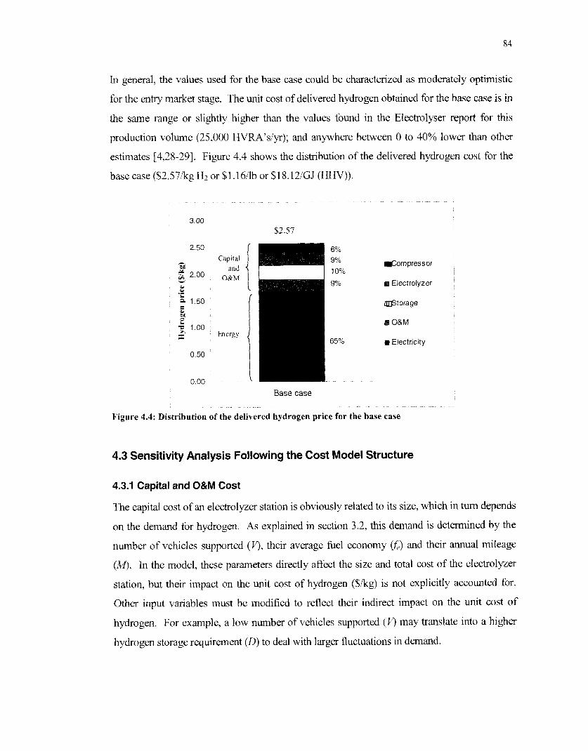
In general, the values used for the base case could be characterized as moderately optimistic
for the entry market stage. The unit cost of delivered hydrogen obtained for the base case is in
the same range or slightly higher than the values found in the Electrolyser report for this
production volume (25,000 HVRA'sJyr); and anywhere between 0 to 40% lower than other
estimates [4,28-291. Figure 4.4 shows the distribution of the delivered hydrogen wst for the
base case ($2.57kg Hz or $l.l6/lb or $18.12/GJ (HHV)).
h Cap~tal
M and 200 O&M 5
E M
-;;, 1 00 Z Energy
Compressor
Electrolyzer
Storage
a O&M
rn Electricity
Base case
Figure 4.4: Distribution of the delivered hydrogen price for the base case
4.3 Sensitivity Analysis Following the Cost Model Structure
4.3.1 Capital and O&M Cost
The capital cost of an electrolyzer station is obviously related to its size, which in turn depends
on the demand for hydrogen. As explained in section 3.2, ths demand is determined by the
number of vehicles supported (V), their average fuel economy Cf,) and their annual mileage
(M). In the model, these parameters directly affect the size and total cost of the electrolyza
station, but their impact on the unit cost of hydrogen ($/kg) is not explicitly accounted for.
Other input variables must be modified to reflect their indirect impact on the unit cost of
hydrogen. For example, a low number of vehicles supported (V) may translate into a lugher
hydrogen storage requirement (D) to deal with larger fluctuations in demand.

Unless specified otherwise, the model assumes the same specific capital cost for the
electrolyzer ($Me), compressor ($/kWOUt) and storage ($/kg H2) components, regardless of
the electrolyzer station's size. This is a reasonable assumption, consistent with DTI's study
[43], considering that the higher specific cost normally associated with smaller units could be
compensated by larger volumes produced.
To help visualize the relative size of electrolyzer stations, table 4.1 gives the hydrogen
production rate, power requirement and approximate footprint for the range considered in this
analysis (2-1000 FCVs supported per station). These estimates are calculated based on a
capacity factor f of 0.7 (operating 70% of the day) and a peak-to-demand ratio Rpd of 1.5, 1.2
and 1.1 respectively for V = 2, 100 and 1000 vehicles supported. The change of peak-to-
demand ratio for each station size explains why their nominal power rating and maximum
hydrogen production rate are not exactly proportional to the number of vehicles supported.
I Electrolyzer station size Number of
vehicles
'able 4.1: Electrolyzer station relative sizes.
Power
@We)
Approximate Footprint
(m2)
' Electrolyzer station: 1
H2 storage: 1-2.5
2~lectrolyzer station: 10-30
H2 storage: 10-20
3~lectrolyzer station: 30-90
Hz storage: 100-200
1 Estimated •’rom Electrolyser report [42]; storage footprint based on enough hydrogen to provide refbelling for two base case FCVs. Considers 2-4 times the area occupied by the compressed gas itself for a 1-metre high volume.
Estimated from Electrolyser report [42]; storage estimated like above, also in agreement with approximate storage footprint in Electrolyser report.
3 Estimated fiom Electrolyser report and Japanese PEM electrolyzer station [42, 511, storage estimated like above.

The parameters directly affecting the "Capital and O&M cost" (C,) in the model are listed in
table 4.2 (with the exception of the electrolyza efficiency q,, included in the Energy cost
section that follows). A range of values for each of these parameters is applied to evaluate the
corresponding sensitivity of the hydrogen cost. The choices of range values are generally
explained in Appendix D. The dominant aspect(s) influenced are identified for discussion in
the second part of the analysis: "T" stands for technical, "E" for economic and "C" for
comparative. Here, parameters of the Capital and O&M cost are associated relatively equally
with the technical and economic aspects.
f eu
Cu
Su
D
A
CRF,
OP
ins
t
Ei
(4
decentralized electrolytic hydrogen dispensing station.
I
Ratio of peak H2 production
to average demand
Capacity factor
Electrolyzer unit cost
Compressor and dispenser unit cost
Hydrogen storage unit cost
Equivalent days of storage
Available fraction of stored hydrogen
Capital recovery factor (effective)
Operation and maintenance
Annual insurance
Annual property taxes
Extraordmry expense E, occurring in year n,
(i= 1,2,3 ...)
Table 4.2: Parameters used to calculate the annual capital and O&M cost (CJ of a I
$/kW,
$ikW,- HHV
$kg H2 storage capacity
d m
% of Ccap
% of Ccw
% of Ccw
$
I
1.1 - 1.5
0.25 - 1
100- 1,000
70 - 500
50 - 500
2- 11.4
0.4 - 1
0.0715 - 0.3280
0.5-4
0-3
0-3
0 - 50% of Ccw every 5
Yem I
1.2
0.7
200
170
200
2
0.5
0.1230
2
1.5
0.5
0
T, E
E, T
T, E
T, E
T, E
T
T
E
T, E
E
E
T, E
I I I

87
Figure 4.5 shows the sensitivity of the unit price of hydrogen to each of theses parameters,
based on the range considered in table 4.2.
Base Rpd f eu cu s u A D CRFe op ins t Ei case
Energy (@ 3LlkWh) Capltal and O&M Sensltrvlty range
Figure 4.5: Sensitivity of hydrogen price to parameters affecting the Capital and O&M cost (C,).
A look at figure 4.5 reveals four dominant parameters that have more impact on the capital
cost of the electrolytic hydrogen station: the effective capital recovery factor CRF,, the
hydrogen storage capacity D, the electrolyzer unit cost e,, and the capacity factor -f: Their
respective sensitivity ranges correspond to 54%, 49%, 42% and 33% of the base case
hydrogen price. In addition to the parameter D, the cost for hydrogen storage is also affected
by s,, and A, suggesting an even greater sensitivity of the hydrogen price to the storage aspect.
Consequently, four items that should be examined more closely in the second part of the
analysis are the financing scheme (related to CRF,), the storage aspect (D, s, and A), the
electrolyzer cost (e,), and the capacity factor 0.
4.3.2 Energy Cost
Table 4.3 shows the list of parameters directly affecting the Energy cost (C,) in the model,
with their respective range considered for sensitivity analysis. This portion is called "Energy
cost" rather than "Electricity cost", to account for the possible use of natural gas in providing
part of the energy required for electrolysis. By appropriate extension, it is even possible to

consider the use of available heat at a fiee cost by adjusting the parameter a (which normally
determines the portion of energy provided by natural gas) as required, and by setting the cost
of natural gas to zero.
The sensitivity of the unit price of hydrogen to each of the "Energy cost" parameters is shown
in figure 4.6, based on the range considered in table 4.3. Again, the choice of minimum and
maximum range values for most parameters is explained in Appendix D.
77c Compressor efficiency % 30 - 100
P e - Electricity price $/kwh 0.01 - 0.07
PNG Natural gas price $lGJ OMV) 3.00 - 8.00
T Electrolysis temperature "C 70 - 1000
Electrolysis pressure
Pi (also inlet pressure to bar 2-414
compressor)
Outlet pressure fi-om compressor bar
Po 2-414 (also hydrogen storage
pressure)
Fraction of energy required for electrolysis -
a 0 - 1 provided by natural gas
(for NGASE)
Table 4.3: Parameters used to calculate the annual energy cost (C,) of a decentralized electrolytic hydrogen dispensing station.
Most of the "Energy cost" variables are associated with the technical aspect, although the one
parameter with the largest impact by far, the electricity price (Pe-), is linked to the economic
aspect (see figure 4.6).
Of the four parameters with a larger impact on the unit price of hydrogen, only two are
associated with conventional electrolysis: the price of electricity (Pe-) and the energy
efficiency of the electrolyzer (qe). Their sensitivity ranges correspond to 131% and 36% of
the base case hydrogen price respectively. In the model, the Capital and O&M cost portion is

also modestly affected by the efficiency of the electrolyzer, which explains a slightly lower
Capital and O&M cost portion for the parameter rl, in figure 4.6.
The other two parameters are the portion of energy provided by natural gas (a) for a
hypothetical commercial version of NGASE, and the price of natural gas (PNG). Their
sensitivity ranges correspond to 37% and 35% of the base case hydrogen price respectively.
For assessing the sensitivity to the natural gas price (PNC), only the case a = 1 was considered,
which explains why the sensitivity range for this parameter does not cover the base case.
Base Pe- PNG T Pi Po case qe qc a
I3 Capltal O&M lil Energy S e n s j t ~ v ~ t y range
Figure 4.6: Sensitivity of hydrogen price to parameters affecting the Energy cost (C,).
The price of electricity (Pe-), the energy efficiency of the electrolyzer (ve) and the potential
impact of using natural gas to provide part of the energy requirement ( a and PNG) should
therefore be the object of more attention in the second part of the analysis.
4.3.3 GHG Added Cost or Saving
The base case does not include any consideration of the GHG aspect; and so far, no "GHG
added cost or saving" component has been included in the sensitivity analysis. Table 4.4
shows the parameters directly affecting the GHG added cost or saving (CCHG) in the model.
For the purpose of this analysis, only two parameters are allowed to vary: the monetary

90
valuation of ,C02 (Eco2) and the electricity mix. The effects of potential he1 economy
improvements are discussed in the second part of the analysis.
saving" ( C G ~ G
Monetary valuation of C02 emissions
Coal Oil
Natural gas Nuclear
Hydroelectric Wind Solar
Other (C02-free)
Fuel economy of FCV with
electrolytic hydrogen FCV with hydrogen fiom decentralized
SMR
Electricity mix
C02-fi.ee mix - 100% coal
co2-free mix
135
(3.02)
kg H2 (gasoline equiv,
U1 OOkm)
Fuel economy of other fuelling options
Methanol FCV with on-board reforming
Gasoline FCV with on-board reforming
gasoline equiv, UlOOkm
Gasoline ICE vehicle
FCV with hydrogen from decentralized co2
equivalent emissions of other fuelling options
rable 4.4: P
SMR
Methanol FCV with on-board reforming
Gasoline FCV with on-board reforming
Gasoline ICE vehicle
rameters used to c, the d cost or associated with a decentralized electrolytic hydrogen dispensing station
All the parameters in table 4.4 are associated with the "comparative" aspect for the second part
of the analysis. The monetary valuation of C02 emissions (Ecor) and the electricity mix are
also associated with the economic aspect, since they both depend to a large extent on
economic considerations. The only parameter associated with the technical aspect that has a
minor indirect effect on the GHG added cost or saving component is the electrolyzer energy

efficiency (G), which is kept constant at the base case value of 80% (HI-IV) for this part of the
sensitivity analysis.
All the base case values for the fuel economy and C02-equivalent emissions of other fuel
options are based on values used in a report written by the Pembina Institute in 2000 [5] to
compare "well-to-wheels" GHG emissions of various fuelling options for FCVs. A
Mercedes-Benz A-Class (5 seats) is used as the reference vehicle for each fuelling option, and
the fuel economy is always calculated based on the U.S. Environmental Protection Agency
(EPA) combined urban and highway driving cycle (45% highway and 55% city driving). The
fuel economy values for an A-Class Mercedes-Benz FCV, running on compressed hydrogen,
methanol or gasoline from an on-board fuel processing system, were obtained fiom Ballard
Power Systems as their "probable case". The &el economy of the gasoline ICE A-Class
Mercedes-Benz was obtained fiom a Mercedes-Benz dealer, based on reformulated gasoline
as the fuel.
The base case fuel economy selected for the compressed hydrogen FCV is 135 kilometres per
kilogram of hydrogen (or 3.02 litres per 100 krn of gasoline equivalent), a value that is within
1% of the projected value by Ballard Power Systems. The same fuel economy value is
therefore applied for both the FCV running on electrolytic hydrogen and the one running on
hydrogen fiom decentralized SMR, since the vehicle sees no difference in the hydrogen
source. See Appendix B for more details on fuel economy conversions.
The so-called "well-to-wheels" GHG emissions include emissions fiom the whole energy
chain, fiom extraction of the fuel to its processing, distribution and final use, as opposed to
tailpipe emissions alone. The Pembina report explains clearly how ernissions at the various
steps were calculated for each fuelling option considered and which reference sources were
used [5].
Figure 4.7 presents the sensitivity of the unit price of hydrogen to the monetary valuation of
C02 and the electricity mix. These two issues are coupled as a monetary valuation of C02 is
necessary to translate in economic terms the advantage of electricity with low GHG emissions.
An increase in C02 monetary valuation merely amplifies the corresponding credit for "clean"
electricity or surtax for "high-GHG" electricity. The graph of figure 4.7 may appear less

92
straightforward to interpret than the previous ones, due to the fact that the "GHG costkaving"
is treated as a relative quantity that can be positive (added cost) or negative (saving).
Sensitivity to electricity mix (from C02 -free mix to 100% coal mix)
for three different monetary evaluations of CQ emission (Em)
100% coal electricit
Cop-free electricity
I
L _ _ Energy H CapitalO&M . Sensitivity range: GHGadded cost or saving 1 -- - . - . - --
Figure 4.7: Sensitivity of hydrogen price to parameters affecting the GHG cost/saving component (CGHG).
Looking at figure 4.7, each "black bar" represents the range of added cost (surtax) - above the
base case line - or saving (credit) - below the base case line - corresponding to the range of
electricity mix. A surtax is calculated when the life-cycle GHG emissions of the electrolytic
hydrogen option are higher than the fuel option to which it is compared. Conversely, a credit
is calculated when the life-cycle GHG emissions are lower than the fuel option to which it is
compared The upper and lower bounds of each "black bar" correspond respectively to
hydrogen produced fiom 100% coal-generated electricity, and fiom C02-fiee electricity.
The magnitude of the sensitivity range is proportional to the monetary valuation of C02
(Eco2); so for a given value of ECO2, the sensitivity range is constant regardless of the fuel
option to which electrolytic hydrogen is compared. In figure 4.7, the sensitivity range for each
of the three C02 monetary valuations of $5/ton, $20/ton and $50/ton corresponds respectively
to 12%, 48%and 1 17% of the base case price of hydrogen.

However, the "breakeven point" between a surtax and a credit shifts progressively as the GHG
emissions of the reference fuel option become lower. For instance, when electrolytic
hydrogen is compared to the gasoline ICE option, a significant portion of the electricity mix
range results in a credit for electrolytic hydrogen (portion of the sensitivity range bar below
the base case hydrogen price line). But when compared to the SMR option, most electricity
mix would result in a surtax (portion of the sensitivity range bar above the base case line).
The cost model gives the possibility to compare electrolyhc hydrogen with four other
reference fuel options, but not explicitly with "hybrid" cars. From a he1 comparison
perspective, hybrid cars can be treated as a sub-case of the gasoline ICE option, with an
improved fuel economy. The magnitude of this improvement can be estimated from
commercially available cars offering both the standard ICE option and the hybrid option, like
the Honda Civic. Based on the fuel economy data for both options [77], a he1 economy
improvement in the order of 25-30% can be expected. As a result, GHG emissions are
approximately equivalent to those of the gasoline FCV option. So with respect to the "GHG
added costhaving" component, the hybrid case is thus equivalent to the gasoline FCV option
in figure 4.7.
The electricity mix and monetary valuation of C02 emissions are discussed further in the
second part of the analysis, along with other issues (not related to GHGs) affecting the
comparative aspect of electrolytic hydrogen.
4.4 Analysis from Three Perspectives
Using the results of the parametric study as a quantitative support, it is now possible to discuss
and contrast the influence of the various issues from a technical, economic and comparative
perspective. Metaphorically, these three perspectives could be seen respectively as those of an
engineer, a businessman and a policymaker (figure 4.8). Each profession archetype sees some
potential benefits in an electrolytic hydrogen fuel infrastructure, but needs a common ground
to discuss the relative importance of the various issues and to get feedback from the other two.
The cost model can provide such a common ground.

Figure 4.8: Perspectives considered in the second part of the analysis.
This section attempts to translate the results from the parametric study into "issues ;" that affect
the competitive position of electrolytic hydrogen as a fuel. The dominant issues in each
perspective are discussed, as well as the effect of the range values used for sensitivity analysis.
First, each of the parameters for which a sensitivity range has been calculated in the previous
section is mapped in a two-dimensional (2-D) space, with the hydrogen price sensitivity on
one axis and the dominant aspect(s) influenced on the other (technical, economic,
comparative). The sensitivity is expressed in percent of the base case hydrogen price, and
categorized in three levels: low (0-20%), medium (20-60%) and high (> 60%). See figure 4.9.
Three elements of caution need to be pointed out in interpreting the results of figure 4.9. One
is that the sensitivity level of a given parameter is directly related to the range of values chosen
for the sensitivity analysis. Although the ranges selected in the study are believed to be
representative of the manoeuvring room available through plausible technical improvements,
market conditions or policy measures, they introduce a subjective element in the analysis. For
example, the sensitivity of the hydrogen price to the electrolyzer unit cost (e,) is based on a
range of 100-1 000 $/kW,, but a narrower range would lower the position of this parameter on
the sensitivity axis. One way around this problem would be to specifl a uniform range of
variation for each parameter (a uniform percentage above and below base case value).
However, this option is hardly applicable here because some parameters can only vary by a
few percent in an actual electrolyzer station, whereas others can vary by orders of magnitude
(e.g. electrolysis pressure), and yet others (like GHG added costkaving) are not even
considered in the base case.

Economic Comparative Technical
High 1 oa -
_-_I_____ -------
for ko2=$ 5 Ofton
10 Low for ECO2 = $5/ton
g -p
Figure 4.9: ~ a ~ ~ i & of parameters in terms of hydrogen price sensitivity and aspects influenced.
The second point to keep in mind is that the parametric sensitivity levels in figure 4.9 reflect
the assumptions contained in the model. For example, the effect of electrolysis temperature
(T) may be underestimated, as the model assumes that all the required energy comes from
electricity, even though a cheaper heat source could provide a sensible portion of the energy at
high temperature.
Finally, the items found in the "comparative" column only reflect the GHG portion of the
comparative aspect. They do not include the effects of other existing fuel taxes or possible
fuel economy improvements for instance. The only two parameters in the comparative

column at this point are the electricity mix and the monetary valuation of C@ (ECO2), which
are presented together since they are coupled in the calculation of the "GHG added cost or
saving". The parameter "electricity mix" appears at three different positions in figure 4.9 to
show how the sensitivity of hydrogen price to the electricity mix increases proportionally to
the monetary valuation of C02.
Notwithstanding these limitations, figure 4.9 provides useful indications about the relative
impact of various issues on the price of electrolytic hydrogen. To translate the impact of
parameters affecting the price of electrolytic hydrogen into "issues", the parameters of figure
4.9 were linked to one or more corresponding issue(s). The result is a list of fifteen distinct
issues listed in table 4.5 below, with their dominant aspect (T-technical, E-economic, C-
comparative). The first nine correspond closely to the issues pointed out in the first part of the
analysis as deserving fiuther attention.
1
2
3
4
5
6
7
Financing scheme & economic parameters
Hydrogen storage
Volume manufactured
Capacity factor
Electricity price
Electrolyzer efficiency
8
9
10
1 1
I I I
Use of natural gas
12 1 Electmlyzer materials
CRFe (& related
D, %,A
%, G, S,
f
pe-
rl e
C02 monetary valuation
Electricity mix
Compression
O&M and extraordinary expenses
13 1 Operating conditions
a, PNG
I I 1 I I %
14
15
X
X
X
k 0 2
"electricity mix"
rlc, CU
op, Ei X
I I I T, Pi, Po
X
X
X
X
X
Table 4.5: List of "issues" associated with the parameters used in the cost model.
Insurance and property taxes
Size of electrolytic hydrogen station
X
X
X
X
ins, t
V, D, Rpd, Pe- X
X
X

These fifteen issues are then mapped in figure 4.10, in a 2-D space similar to the one used for
the parametric sensitivity analysis (figure 4.9). The potential impact mgh, medium or low) of
each issue corresponds to the sensitivity found for the associated parameter(s) in figure 4.9.
When more than one parameter is linked to an issue, the sensitivity of hydrogen price to that
particular issue reflects the compounded sensitivity to the related parameters.
IMPACT Technical Economic Comparative
High
Medium
Low
Figure 4.10:
For the ele
reflect the
transaction,

ascribed to a compliance cost for emission reduction. It should be noted though that this is, at
best, only a lower bound for the true marginal external cost of C02 emissions.
Based on the results of figure 4.10, the issues with the most impact on the competitive position
of electrolytic hydrogen are briefly discussed in the following three subsections, while others
are simply touched on, considering the limited scope of this analysis.
4.4.1 Influences from a Technical Perspective
4.4.1.1 Hydrogen Storage
Surprisingly, the technical issue that ranks highest in figure 4.10 is hydrogen storage. There
are a few reasons explaining why hydrogen storage has more impact than any other technical
issue in thts analysis. First, the study only considered electrolyzer stations offering the same
convenience of fast refuelling as gasoline. This implies that sufficient quantities of hydrogen
have to be stored at the fuelling station site to support a "fast fill" mode. Second, only the
high-pressure gaseous hydrogen storage option was considered here, with its associated
technical and economic limitations.
In this analysis, the storage requirements are determined by the quantity deemed sufficient to
provide "fast fill" convenience for a given station size, and by the fraction of stored hydrogen
which is available in practice. The former is expressed in the model by the parameter D, in
equivalent days of nominal production, and the latter by the parameter A, giving the available
fi-action of hydrogen stored.
The selected range of values for the parameter D in the sensitivity analysis is 2-1 1.4, reflecting
some assumptions made in the DTI report for hydrogen storage requirements as a function of
station size [43]. The maximum range value D =11.4 corresponds to the smallest electrolyzer
station considered in this study, i.e. a personal appliance supporting the hydrogen needs of two
FCVs. This value is obtained by assuming two FCV tanks' worth of usable hydrogen storage.
In other words, it would take 11.4 days at the nominal hydrogen production rate (determined
by average daily consumption) to produce enough hydrogen to fill completely the hydrogen
tanks of two FCVs.
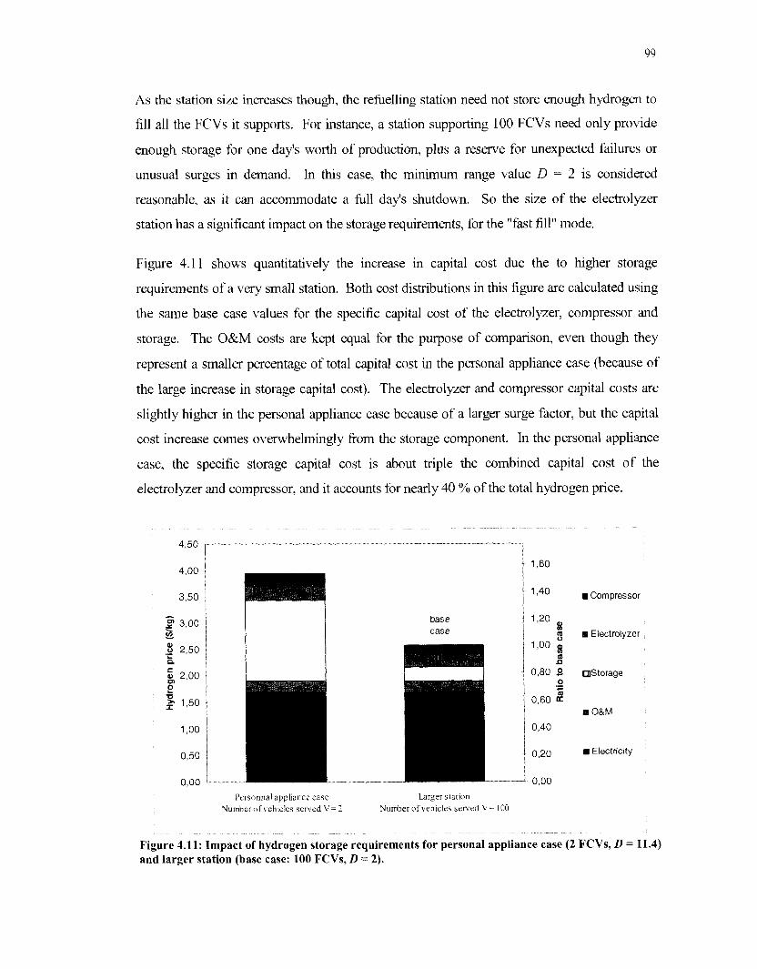
As the station size increases though, the refuelling station need not store enough hydrogen to
fill all the FCVs it supports. For instance, a station supporting 100 FCVs need only provide
enough storage for one day's worth of production, plus a reserve for unexpected failures or
unusual surges in demand. In ths case, the minimum range value D = 2 is considered
reasonable, as it can accommodate a full day's shutdown. So the size of the electrolyzer
station has a significant impact on the storage requirements, for the "fast fill" mode.
Figure 4.1 1 shows quantitatively the increase in capital cost due the to higher storage
requirements of a very small station. Both cost distributions in ths figure are calculated using
the same base case values for the specific capital cost of the electrolyzer, compressor and
storage. The O&M costs are kept equal for the purpose of comparison, even though they
represent a smaller percentage of total capital cost in the personal appliance case (because of
the large increase in storage capital cost). The electrolyzer and compressor capital costs are
slightly hgher in the personal appliance case because of a larger surge factor, but the capital
cost increase comes overwhelmingly from the storage component. In the personal appliance
case, the specific storage capital cost is about triple the combined capital cost of the
electrolyzer and compressor, and it accounts for nearly 40 % of the total hydrogen price.
base case
Personnal appliance case Larger station Number ofveh~cles served V = 2 Number of veh~cles served V = 100
8 Compressor
Electrolyzer
Storage
a O&M
r Electncrty
Figure 4.11: Impact of hydrogen storage requirements for personal appliance case (2 FCVs, D = 11.4) and larger station (base case: 100 FCVs, D = 2).

The Electrolyser report avoided the large capital cost associated with storage for the personal
appliance case, by considering only the "time fill" option, i.e. hydrogen stored directly
onboard the FCV as it is produced. This analysis did not consider the "time fill" option,
because it increases the refuelling time significantly and can limit the driving range. These
limitations are accentuated for a small station. With the "time fill" option, a FCV fuelled by a
personal appliance could not travel a long distance two days in a row, because the electrolyzer
would then take a few days to produce enough hydrogen to fill the tank again.
One disadvantage of compressed hydrogen storage is that a significant portion of the hydrogen
always remains in the storage tanks, because pressure in the station storage vessels goes down
while it increases in the FCV tanks during transfer of hydrogen. Thomas et al. suggest that
hydrogen should be dispersed in at least three separate refueling tanks to provide cascade
filling of the FCV tank, i.e. the vehicle tank would be filled first fi-om the lowest-pressure
storage vessel, moving in succession to the highest-pressure vessel to assure maximum mass
flow and minimum compression energy. But even with multiple tanks and cascade filling of
the FCV, at best 60% of the stored hydrogen can be utilized [43]. That is why the base case
assumed only 50% of the stored hydrogen is usable (parameter A = 0.5). The net effect is that
the storage volume needs to be twice the size (and cost) of what is really required in terms of
stored hydrogen. Private discussions with a company active in the design of hydrogen
refuelling stations indicated that the fi-action of usable hydrogen could be increased up to the
90% level by clever cascading of tanks and the use of a small compressor.
The high specific capital cost of compressed hydrogen storage (parameter s,) accentuates the
effects of storage requirements discussed above. Indeed, compressed-gas storage is rather
expensive, particularly when compared to storage for liquid fuels like gasoline. Various
sources in the literature provide useful estimates for the capital cost of high-pressure storage
tanks (350-400 bars). They are generally in the range of 300-500 $/kg Hz, but can go over
1000 $/kg H2 [28,29,43]. For the sensitivity analysis, a relatively optimistic base case value
of 200 $/kg H2 was used. This value lies somewhere between the projected value used in the
DTI report (132 $/kg) [43] for advanced carbon fiber tanks, and the value used in the
Electrolyser report (3 57 $/kg) based on commercially available tanks [42].

Some of the assumptions regarding hydrogen storage may have emphasized its impact on the
price of hydrogen; nevertheless the analysis stresses the importance of this issue in planning a
hydrogen helling infi-astructure for FCVs. Based on these results, here are four possible
avenues to restrain the impact of storage:
Eliminate stationary hydrogen storage by making the "time fill" option acceptable. One
particularly ambitious approach is to have a small electrolyzer directly onboard FCVs, to
produce hydrogen wherever the FCV can be connected to the electric grid, provided there
exists a convenient way to bill this electricity to the user.
Favor electrolyzer stations that support a larger fleet of FCVs, to minimize the storage
requirements. (Minimize parameter D)
Use a compressor to optimize the fi-action of usable stored hydrogen. (parameter A). This
compressor could be the same as the one used for compressing hydrogen in the first place.
Develop inexpensive hydrogen storage technology.
4.4.1.2 Electrolyzer
The sensitivity analysis suggests that the electrolyzer eficiency (G) is the issue that has the
most impact among those directly related to the electrolyzer. That is because the amount of
electricity required (whch is the dominant cost in electrolyhc hydrogen) is directly related to
the energy efficiency of the electrolyzer. Also, the more efficient an electrolyzer is, the
smaller it has to be to deliver a given flow rate of hydrogen.
The actual impact of electrolyzer efficiency could be less than suggested in the sensitivity
analysis however. First because most electrolytic cells commercially available today can
already operate at a relatively hgh energy efficiency (80-90% HHV), so the available room
there is limited. Also, for the purpose of the sensitivity analysis, the model assumes a constant
specific capital cost of electrolyzer ($/kW) regardless of efficiency, with the net result that a
more efficient electrolyzer is smaller and proportionally less expensive. In reality, an
improved energy efficiency would likely imply a hgher specific capital cost of electrolyzer,
offsetting the cost reduction, partially or completely.

One surprising result of the sensitivity analysis is the low impact of operating conditions, such
as the temperature and pressure at which water electrolysis takes place. Their impact on the
price of electrolytic hydrogen may have been minimized here because of some assumptions
contained in the model, yet the results suggest that an optimization of operating conditions
would have only a limited effect on the price of electrolytic hydrogen.
With respect to temperature, the model focused on the resulting energy requirements based on
thermodynamic considerations only, but it did not consider explicitly some indirect potential
benefits. For instance, it does not reflect efficiency improvements associated with higher
operating temperature, nor does it consider the 111 benefits of high temperature electrolysis
(HTE). Because all the required energy (even heat) is assumed to come from electricity in the
sensitivity analysis, the net effect on the energy component of the hydrogen cost is very small.
In principle though, the use of free heat in HTE could cut the energy cost of water electrolysis
by up to 25%, as pointed out in Chapter 2.
The effects of electrolysis pressure may also have been minimized in the analysis because of
some assumptions contained in the model. In terms of capital costs, the model does not
explicitly consider an increased electrolyser cost (eJ with higher operating pressure, nor does
it consider a lower compressor capital cost (c,,), since the compressor unit cost is based on the
hydrogen flow and not the degree of compression. In terms of energy, the model does not
consider any increase in efficiency with hgher pressure, and it assumes a constant value of
100% for current efficiency. This is a valid approximation at low pressure, but the cunent
efficiency tends to decrease at higher operating pressure.
The specific capital cost of the electrolyzer p a kW, (e,) is influenced more by the volume
manufactured (primarily an economic issue) than by the materials used in the electrolyhc cells.
So even if the cost of electrolytic cells were reduced by half or more, by using inexpensive
materials, the overall impact on hydrogen cost would be only a few percents. A review of the
cost distribution for various electrolyzer station sizes in the Electrolyser report [42] indicates
that simplification and cost reduction in the power and water conditioning systems could have
a comparable impact on the capital cost of the electrolyzer.
The issue of O M and extraordinary expenses has not been addressed with much detail, due
to its relatively low impact in the sensitivity analysis. However some items are worth pointing
out. From the estimates found in the Electrolyser report, 60-90% of the O&M costs are
related to the compressor and water purifier components. Also, O&M annual costs generally
represent a larger percentage (up to 57%) of the capital costs for smaller electrolyzer stations.
4.4.1.3 Compression
Figure 4.10 shows that the compression issue has only a moderate impact on the price of
hydrogen. Thls impact reflects the combined sensitivity of hydrogen price to the capital cost
of the compressor (c,) and the energy efficiency of compression (q). Some couplings are not
explicitly reflected in the model, such as higher O&M costs and a likely hgher specific capital
cost ($/kW, HHV) associated with more intensive compression. But the range values used
in the sensitivity analysis are believed to cover these simplifications.
The maximum value considered for the output pressure fiom the compressor (Po) was limited
at 414 bars (6000 psi) because it appeared to be a practical limit for commercial applications
of hydrogen storage. However, recent work on hydrogen storage for FCVs is pushing this
limit towards 700 bars (10000 psi). If this were to become commercially viable, the
compression issue could have a slightly higher impact on the hydrogen price. At this pressure
level, hydrogen can no longer be approximated as an ideal gas (like it is the case in the cost
model), so the model would underestimate the energy use related to compression. The trade-
offs between electrolysis pressure and compression are discussed in Chapter 2.
4.4.1.4 Use of Natural Gas
The sensitivity analysis confirmed that natural gas assisted steam electrolysis (NGASE) could
be a promising avenue for reducing the cost of electrolybc hydrogen. However, given the
trend of intensive developments in small-scale SMR, it is unlikely that NGASE will reach the
commercial stage. That is because small-scale SMR promises similar or higher performance
in terms of energy efficiency (up to 80% HHV) [29], and it is already the focus of much
development for processing the natural gas used in stationary fuel cell systems. The main
advantage of NGASE vs. small-scale SMR would be the ability to use both electricity and
natural gas. The principles of NGASE are summarized in section 2.3.1.
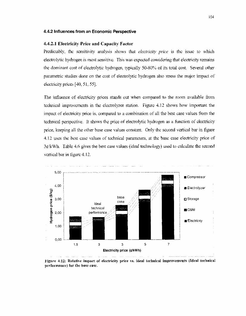
4.4.2 Influences from an Economic Perspective
4.4.2.1 Electricity Price and Capacity Factor
Predictably, the sensitivity analysis shows that electricity price is the issue to which
electrolytic hydrogen is most sensitive. This was expected considering that electricity remains
the dominant cost of electrolytic hydrogen, typically 50-80% of its total cost. Several other
parametric studies done on the cost of electrolytic hydrogen also stress the major impact of
electricity prices [40,51,55].
The influence of electricity prices stands out when compared to the room available from
technical improvements in the electrolyzer station. Figure 4.12 shows how important the
impact of elechlcity price is, compared to a combination of all the best case values from the
technical perspective. It shows the price of electrolytic hydrogen as a fbnction of electricity
price, keeping all the other base case values constant. Only the second vertical bar in figure
4.12 uses the best case values of techcal parameters, at the base case electricity price of
3ClkWh. Table 4.6 gives the best case values (ideal technology) used to calculate the second
vertical bar in figure 4.12.
Compressor
Electrolyzer
Storage
O&M
Electricity
1,5 3 3 5 7
Electricity price ((t/kW h)
Figure 4.12: Relative impact of electricity price vs. ideal technical improvements (Ideal technical performance) for the base case.

- eu
CU
SU
A
OP
rle
rlc
Table 4.6: Values used to estimate the maximum cost reduction achievable through technical improvements.
A
OP
Ve
Compressor and
In the base case cost distribution of electrolytic hydrogen (third vertical bar of figure 4.12)
electricity at 3 $/kwh represents 65% of the total cost. A convenient way to highlight the
importance of electricity price is to express the remaining 35% (capital and O&M costs) in
tenns of electricity price. For the base case values, this would be equivalent to 1.6 $/kwh for
capital and O&M costs. So the total price of electrolflc hydrogen can be thought of in
general as proportional to the electricity price plus 1-3 $/kWh for capital and O&M costs.
Electrolyzer unit cost Compressor and
dispenser unit cost
Hydrogen storage unit cost
Available hction of stored hydrogen Operation and maintenance
Energy efficiency of electrolyzer Compressor efficiency
The main challenge for electrolytic hydrogen is therefore to identifL strategies that minimize
the electricity price. A general understanding of the electricity market's dynamics is helphl to
see how water electrolysis can take advantage of it. Electric utilities must supply very reliable
electricity under widely fluctuating load conditions. For example, the average ratio of
minimum hourly demand to peak demand on a daily basis is in the order of 40-50% for
American utilities [43]. A consistent large gap between peak load and night-time load
characterizes the demand pattern of most utilities. To ensure system reliability, North
American utilities must follow strict guidelines, requiring them to maintain different operating
reserves, including a spinning reserve accessible instantaneously and a non-spinning reserve
accessible w i t h ten minutes.
Available hction of stored hydrogen Operation and maintenance
Energy efficiency of
I $kWm
The "load characteristics" of the electrolysis process put it in an excellent position to take
advantage of the mismatch between electricity supply and demand. Unllke many other
industrial loads, water electrolysis can be interrupted and operated intermittently without
$kWe $kWm -HHV
$ k H2 storage capacity
% of CCUD
%
%
CapdCllY
% of CCUD
OL
100
I 70
100
70
200
170
1
0.5
I nn
-50%
-59%
200
170
-50%
-59%
50 200 -75%
0.5
2
80
1
0.5
100
100
+ 100%
-75%
+25%
0.5
2
80
75
+ 100%
-75%
+25%
+33%

upsetting the basic hydrogen production process. Also, the process does not require high
quality power. These characteristics offer the prospect of a large-scale integration of
electricity generation and hydrogen production. Utilities could manage distributed
electrolyzers as a "recallable" load, i.e. a power supply which can be interrupted when needed.
In fact, the process could even qualifL as a non-spinning operating reserve for utilities [42].
This type of approach allowing utilities to manage the time at which they provide electricity to
electrolyzers, would favor very low cost electricity.
Because of hydrogen storage, electrolyzers can maximize the use of inexpensive excess
electricity during off-peak periods. Off-peak electricity represents a key opportunity for low-
cost electricity in many locations. This is particularly true for utilities largely dependent on
coal or nuclear power generation, because it is often less costly in these cases to let the
generator run in off-peak periods than to turn off the process. Based on a survey of American
electric utilities, Thomas and Kuhn found out that most utilities have a marginal operating cost
(the cost of fuel and other maintenance costs associated with adding extra electrical output at
any instant of time) that is consistently below 2 $/kWh during night time [43]. It is therefore
reasonable to conclude that many utilities could still recover some of their capital investments
by providing electricity around 3$/kWh during off-peak periods.
Due to its high impact on the price of electrolytic hydrogen, off-peak electricity can be the
determinant element for selecting the capacity factor of the electrolyzer. That is why the
capacity factor issue is discussed along with electricity price in this section. For example, an
electrolyzer designed to operate 16 hours a day on average will have a capacity factor of 0.67
(16h124h), but an electrolyzer designed to take advantage of off-peak electricity rates may be
designed to operate only 8 hours a day with a corresponding capacity factor of 0.33 (8hl24h).
In the latter case, the electrolyzer would have to be designed twice as big to accommodate
double the hydrogen production rate. In the sensitivity analysis, the net result is a doubling of
the capital cost of the electrolyzer and compressor (but not storage). Doubling the capital cost
of these two items in the base case is equivalent to increasing the electricity price by
0.7$/kWh. So if the average electricity price goes down by at least 0.7$/kWh by using off-
peak rates only, it is then worth it to increase the capital cost of the electrolyzer. This kind of
trade-off must be considered when selecting the capacity factor of an electrolyzer station.

Electrolytic hydrogen fiom renewable energy sources (hydro, wind, solar.. .) is the long-term
objective to minimize GHG emissions and other polluting emissions. Among the renewable
options, only hydroelectricity can compete economically today with other large-scale power
generation methods. But a very limited number of regions around the world (e.g. British
Columbia) have access to abundant inexpensive hydroelectricity. There are also few
incentives for utilities to sell off-peak electricity fiom hydro power, since dams can be
controlled to store water for peak demand periods and exports. Nevertheless, some utilities
like BC Hydro are working on a development strategy to provide decentralized electrolytic
hydrogen, based on time-of-use electricity at prices as low as 2.4 $kWh (3.1 $/kWh CAN)
[78]. Wind energy also presents some interesting potential in the short to mid-term,
particularly if some credits are granted to encourage its development. An example is the
special credit of 1.299kWl-1 for wind energy available in Canada since 2001.
So to summarize, here are some avenues to increase access to low-cost electricity:
Optimize access to off-peak electricity by establishing new better adapted tariff structures
for off-peak electricity.
Take advantage of the interruptible nature of water electrolysis to use existing operating
reserves at low rates, with limited additional GHG emissions. Spinning reserves in North
America amount to approximately 15 GW (2% of the potential generating capacity),
which represents enough electricity to produce 2.3 million tons of electrolytic hydrogen
annually, or enough hydrogen to he1 over 10 million FCVs [42].
Offer fiscal incentives for hydrogen produced fiom electricity with low GHG emissions.
4.4.2.2 Financing Scheme and Economic Parameters
In the cost model, the total installed capital cost of an electrolyzer station is calculated
independently of the way it is financed. But the actual annual expense associated with this
capital cost depends on the effective capital recovery factor (CRFe), which incorporates the
effects of all economic parameters that influence the financing. The CRFe acts as a
multiplying factor of the totalled installed capital cost to determine the actual annual cost of
the capital assets. For example, a CRFe = 0.15 means that the annual expense attributed to
capital cost corresponds to 15% of the total installed capital cost.

As explained in the cost model description, three financing scenarios were envisioned:
financed by the consumer as a home mortgage (applicable to very small stations only), by a
business, and by a utility. A base case was developed for each of these financing scenarios
(Table 4.7) and a sensitivity analysis performed on the relevant parameters to see how the
CRFe is affected (Figure 4.1 3). The base case values are nearly all identical to those used by
Thomas and Kuhn [43]. The CRFe base case value of 0.1230 used throughout this study
corresponds to the "utility base case" below.
IN I Economic recovery period 5 - 30 I 15 I
l i l General inflation rate 1 % 1 0 - 15 I B: 2.7 U: 2.7 I
im
Table 4.7: Parameters affecting the effective capital recovery factor (CRF,)
Personal tax rate of owner % 25 - 50 H: 35
Mortgage interest rate
y
Tb
Base cases IE4 Minimum Sensistivity range
Figure 4.13: Sensitivity of the effective capital recovery factor (CFW,) to various economic parameters under three different financing scenarios (B: business, U: utility, H: home mortgage)
%
After-tax real rate of return on investment
Business tax rate
5-15
%
%
H: 9
4- 15
0 -50
B: 10 U. 6
B: 26 U: 0

The most important result of figure 4.13 is that the value of CRFe can vary by as much as a
factor of three (fiom less than 0.10 to over 0.30). In other words, the portion of hydrogen
price that covers the electrolyzer station's capital cost can vary by a factor of three, simply on
the basis of the financing scheme and economic parameters.
Looking at the main sensitivity results of figure 4.13, the economic recovery period (N) has a
relatively high impact, but extending its value beyond the base case value of 15 years has very
little effect. The rate of return on investment (r) has more impact in the "business" scenario
than the "utility" scenario because the expected rate of return would likely be lower for a
utility. That assumption is justified essentially by the fact that the opportunity for a utility lies
more in additional sales of electricity than the electrolyzer station itself, which is not the case
for the "business" scenario. Finally, the impact of inflation in the "business" and "utility"
scenarios highlight the importance of stable economic conditions to minimize the capital cost.
Figure 4.13 indicates that the "home owner" financing scenario could be the least expensive
(CRFe = 0.1020 for base case "H") followed closely by the "utility" scenario (CRFe = 0.1230
for base case "U"). However, since the "home owner" scenario applies only to very small
electrolyzer stations with higher storage requirements, the "utility" scenario may turn out to be
the most advantageous one as suggested in figure 4.14.
So having electrolyzer stations financed by a power utility appears to be the best scenario for
at least three reasons.
Utilities can afford a lower expected rate of return on the electrolyzer stations, because
their main financial interest comes fiom additional sales of electricity, which constitutes
their core business. Also, utilities themselves generally have access to low-cost financing.
Utilities could offer the flexibility that is necessary to adapt to an evolving market for
electrolyhc hydrogen. As the demand increases, a utility could replace small electrolyzers
by larger ones and move the smaller ones to locations with lower demand. Electrolyzer
stations of proper capacity would then be amortized over their 111 economic life.
The capital cost of multiple electrolyzer stations could then be averaged, the most
profitable stations compensating for the ones with a low utilization.

Compressor
Electrolyzer
Storage
. O&M
Electric~ty
Busme5s 15-year lJt111ty 15-year Mortgage 25- Utlllty 15-year Ruslness 15-year loan loan a I loan loan
Personnal appl~ance case Larger s tatlon N u d e r of vehicles served V = 2 N u d e r ofvehicles served V = 100
Figure 4.14: Impact of financing scenario on hydrogen price for two different sizes of electrolyzer stations. The unit capital cost of electrolyzer, compressor and storage components are the same for the two sizes. O&M represents the same Oh of capital cost for each electrolyzer station's size.
4.4.2.3 Other Economic Issues
Figure 4.10 suggests that the volume of electrolyzer stations manufactured is the economic
issue with the next most important impact on hydrogen price, after the electricity price and
financing scheme. The range values in the sensitivity analysis for the unit cost of the
electrolyzer, compressor and storage components (e, ,c, and s,) were estimated without
distinguishing between the impact of inexpensive materials, simpler design and larger volume.
However, other studies have looked more specifically at the impact of volume for electrolytic
hydrogen fhelling stations, and show an important drop in capital cost with increasing volume
[4, 421. The graph below (figure 4.15) comes fi-om one of these studies. For a station
supporting 100 FCVs and an electricity price of 3$'kWh, both quantities equal to the base case
of this study, this graph shows that increasing the volume of electrolyzers from 100 to ZOO0
units results in a decrease in hydrogen price ii-om approximately 4$kg to 3$/kg, i.e. about
25% reduction.
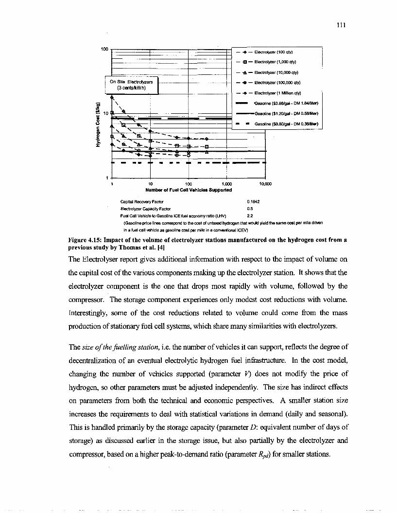
I I I I
I I - Q - Electrolyzer (1.000 qty)
On Site Electroiyrers ---- - ---------- - - + - ~~ectm~y le r ( i o o , ~ sty) (3 centskW h) - 4 - Electrolyzer (1 MIIMm qty)
1 10 100 1,000 10,000
Number of Fuel Cell Vehicles Supported
Capital Rewvecy Factor 0.1842
Electrolyzer Capacity Factor 0.5
Fuel Cell Vehide to Gasoline ICE fuel economy ratio (LHV) 2.2
(Gasoline price lines correspond to the cost of untaxed hydrogen that would yield the same cost per mile drlven
in a fuel cell vehicle as gasoline cwt per mile in a comrentional ICRI)
Figure 4.15: Impact of the volume of electrolyzer stations manufactured on the hydrogen cost from a previous study by Thomas et al. [4]
The Electrolyser report gives additional information with respect to the impact of volume on
the capital cost of the various components making up the electrolyzer station. It shows that the
electrolyzer component is the one that drops most rapidly with volume, followed by the
compressor. The storage component experiences only modest cost reductions with volume.
Interestingly, some of the cost reductions related to volume could come from the mass
production of stationary he1 cell systems, which share many similarities with electrolyzers.
The size of the fuelling station, i.e. the number of vehicles it can support, reflects the degree of
decentralization of an eventual electrolyhc hydrogen he1 infrastructure. In the cost model,
changing the number of vehcles supported (parameter V) does not modify the price of
hydrogen, so other parameters must be adjusted independently. The size has indirect effects
on parameters fiom both the techcal and economic perspectives. A smaller station size
increases the requirements to deal with statistical variations in demand (daily and seasonal).
Thls is handled primarily by the storage capacity (parameter D: equivalent number of days of
storage) as discussed earlier in the storage issue, but also partially by the electrolyzer and
compressor, based on a higher peak-to-demand ratio (parameter Rpd) for smaller stations.

There is no definite relationship between electrolyzer size and electricity price, because it can
vary in so many different ways, according to local electricity rate schedules. But residential
electricity rates for small applications are generally higher than those for larger industrial
applications. So larger electrolyzers could be expected to benefit from lower electricity prices,
unless a particular tariff structure is put in place to give equal access to low electricity rates.
Finally, the utilization of the electrolyzer station is another factor that can be linked to its size.
In the cost model, the station's size is function of the number of vehicles supported.
Accordingly, the capital cost is amortized over the total projected hydrogen production. In
reality though, there could be fewer vehcles to support than actually projected. For instance,
if a station designed to support 100 FCVs serves only 50 FCVs on average during its initial
years, it is utilized only at 50% of its rated production. The capital cost must then be
amortized over half the projected production to remain profitable. The net effect is a doubling
of the portion of hydrogen price assigned to cover the amortization of the station's capital cost.
Thus, even if the capital cost of smaller station appears higher (per unit of hydrogen
produced), it could still be more economical to add production capacity as needed, than invest
in a larger electrolyzer station that is under-utilized.
4.4.3 Influences from a Comparative Perspective
Thus far, technical and economic issues that directly influence the cost of electrolytic
hydrogen have been discussed, but the competitive position of hydrogen also depends on its
price relative to other he1 alternatives. An in-depth look at the cost of other fuelling options is
clearly outside the scope of this research. However, it is possible to estimate the impact of
some indirect issues affecting the competitive position of hydrogen. One such issue that has
been addressed already in the sensitivity analysis is the impact of a GHG Wcredit reflecting
the combined effect of C02 monetary valuation and electricity mix. This GHG Wcredit is
further discussed in h s section as well as other existing he1 taxes. The effect of potential fuel
economy improvements of other fuel options is also considered.
To illustrate concretely the impact of these issues on the competitive position of hydrogen,
actual information fi-om three cities was used. These three cities (Vancouver, Los Angeles,
and Paris) present fairly different electricity mix, electricity rates and he1 taxes.

4.4.3.1 C02 Emissions and Monetary Valuation
One of the objectives of this research was to get a sense of the economic advantage of "clean"
electrolytic hydrogen (very low associated C02 emissions) versus other kelling options for
FCVs. To estimate this, the cost model calculates the life-cycle GHG emissions (on a per-
kilometer basis) associated on the one hand with a FCV using electrolytic hydrogen, and on
the other hand with the equivalent vehicle using the alternative fuel option considered. The
difference between the two is then assigned an economic value proportional to the monetary
valuation of C02. If the GHG emissions from electrolytic hydrogen are lower than the
alternative option, then the model calculates a theoretical credit for electrolytic hydrogen; if
they are higher, the model calculates a theoretical surtax. So both the electricity mix and COz
monetary valuation affect the magnitude of this economic advantage (credit) or disadvantage
(surtax) of electrolytic hydrogen versus an alternative fuel option.
Figure 4.16 shows the life-cycle GHG emissions associated with each fuel option considered
in the cost model. The calculated GHG emissions are based on a previous study done by the
Pembina Institute for Appropriate Development [ 5 ] . The GHG emissions associated with
electrolytic hydrogen vary widely fkom 0 to 450 grams of C02 per kilometer, as a fhction of
the electricity mix.
Electricity from 100% coal
Electricity from 100% oil
Electricity from 100% natura
0
0 200 400 600 800 1000
C02 emissions from electricity mix (g CO21kWh)
-H2 FCVfrom electrolysis (3.02 litre1100 km)
H2 FCVfrom SMR (3.02 litrell 00 km)
Methanol FCV (4.1 9 lttrell 00 km)
Gasoline FCV (6.1 1 litref1 00 km )
Gasoline ICE (7.30 litrell 00 km)
Figure 4.16: Life-cycle COz emissions per kilometer from a FCV using electrolytic hydrogen as a function of electricity mix (solid line), compared to C 0 2 emissions of other fuel options.

Figure 4.16 highlights the fact that electrolytic hydrogen produced fiom fossil fuel-based
electricity (coal, oil, or even natural gas) would result in higher life-cycle GHG emissions than
any other fuel option considered, despite the better fuel economy of hydrogen-fuelled FCVs.
Yet, in many countries most of the electricity comes fiom fossil fbels. For example, the
average electricity mix in the United States produces 650 grams of C02/kWh [79]. Hence, a
FCV running on electrolytic hydrogen produced fiom the average electricity mix in the United
States would have higher C02 emissions than a comparable internal combustion engine (ICE)
vehicle running on gasoline.
As indicated by figure 4.16, for water electrolysis to compete with hydrogen fiom
decentralized SMR in terms of GHG emissions, the electricity mix needs to emit less than 205
grams of C02/kWh, corresponding to a mix of 35% electricity from natural gas, and the rest
fiom C02-fiee electricity. The use of electricity fiom spinning reserves could be an exception
to the high C02 emissions associated with electrolytic hydrogen from fossil-based electricity.
That could be justified by the fact that most of the associated C02 emissions would be
produced regardless, to ensure the reliability of the electricity network.
To foster a shR towards technologies with low associated GHG emissions, a monetary value
must be assigned to C02; whether it is determined by policy, the market, or a combination of
the two. Otherwise, there is no incentive fiom an economic standpoint to even consider GHG
emissions in selecting a fuel option for future FCVs. As seen in the sensitivity graph for the
"GHG added costlsaving" (figure 4.7), the monetary valuation of C02 can have a sizeable
impact on the competitive position of electrolytic hydrogen, if it is high enough. The value
$20/ton of C02 (equivalent to $73/ton of carbon) was selected to estimate the maximum
impact of C02 monetary valuation, resulting in a "medium" impact on the competitive
position of electrolytic hydrogen (figure 4.10). This value appears to be a realistic upper limit,
based on recent price projections for the next decade [20] and actual transactions that have
taken place so far in pilot projects.
A useful way to estimate the economic impact of C02 monetary valuation is to know that a
value of $1 Olton of C02, applied literally to the range of electricity mix, creates a differential
of about 1 $/kwh, in favor of C02-free electricity versus coal generated electricity.

4.4.3.2 Comparison of Electrolytic Hydrogen and Gasoline in Three Locations
The cost model developed offas enough flexibility to compare the cost of electrolytic
hydrogen and other fuel options in any location. In this concise analysis though, it is
obviously impossible to cover all the fuel options in details, let alone a wide array of locations.
This is better done in other studies [45]. So the focus of this section has been limited to a
comparison between electrolytic hydrogen and gasoline in three cities: Vancouver (Canada),
Los Angeles (United States), and Paris (France). These cities were chosen for their different
electricity mix, electricity tariffs and he1 taxes, to illustrate the effects of geographic location.
The same base case electrolyser station, designed to serve 100 vehicles and assumed to have
the exact same total installed capital cost, is placed in each location. The fuelling cost for the
two he1 options in each city is calculated based on an equivalent driving range for the
hydrogen FCV and gasoline ICE vehicle. The data used for calculating the helling costs is
presented in table 4.8 below, with the relevant sources available in Appendix E. The results
are shown in figure 4.17
* Electricity price I I I US&^&%) I 3.2
* Electricity priqes calculated using local tariff schedule for an electrolyzer station supporting 100 hydrogen FCVs, with a capacity factor of 0.7.
t Tax on fie1 (US$lGJ)
t Hydrogen taxed at same rate as on gasoline, on an energy content basis (HHV).
12.8
COP monetary valuation I US$2O/ton C02-equivalent
5.9 Electricity mix I Dominated by
hydroelectric (93%)
5.98
Height of triangle arrows ('I) in figure 4.17 indicates the magnitude of the credit that could be applied to electrolyhc hydrogen for reducing GHG emissions compared to gasoline, at US$2O/ton C02-equivalent
Dominated by NG (50%) and coal (1 1%)
2.90
Hydrogen FCV: 3.02 liter 11 00 km (gasoline equivalent) corresponds to 135 km kg H2
Dominated by nuclear (82%)
27.23
Vehicle range
Fuel economy
Table 4.8: Assumptions and values used for the cost comparison of electrolytic hydrogen with gasoline in three cities.
600 km/full tank on EPA combined driving cycle (Identical for both the gasoline ICE vehicle and the hydrogen FCV)
Gasoline ICE vehicle: 7.30 liter I1 00 km

Gasoline H2
Vancouver
Gasoline H2 Gasoline H2
Los Angeles Paris
Figure 4.17: Site-specific comparison of gasoline and electrolytic hydrogen retail price including taxes and the effect of credits for low CO, emissions.
The first interesting observation is that electrolytic hydrogen would be competitive with
gasoline in two of these three locations: Vancouver and Paris, even if it is taxed at the same
rate as gasoline. In Vancouver, the low electricity rate is mostly responsible for this result,
whereas in Paris it is the high &el tax that really makes a difference. Notice that even if the
electrolyzer capital and O&M costs were doubled in these two locations, electrolytic hydrogen
could still compete with gasoline. In Los Angeles though, electrolytic hydrogen would be
more than twice as expensive as gasoline, due to a combination of low he1 tax and high
electricity rates. Vancouver and Paris, which have lower priced electricity, also happen to be
the ones with the lowest GHG emissions. So a COz credit would simply reinforce the
competitive position of electrolytic hydrogen in these locations, whereas it would have almost
no effect in Los Angeles.
For each location:
These issues are fixther discussed in the next three sub-sections, and generalized to see what
levels of ke l tax and electricity prices can produce an economic breakeven condition between
electrolytic hydrogen for a FCV and gasoline for an ICE vehicle.
Gasoline Retail Price Hydrogen Retail Price Effect of C02 evaluation
Fuel Tax Fuel Tax Credit (r )or Added Tax (A )
Untaxed Gasoline rn Electricity
Electrolyzer Capital + O&M
4.4.3.2.1 Electricity Price and Mix As shown in figure 4.17, the average electricity price varies widely fiom 3.2 $kWh in
Vancouver to 12.8 $/kwh in Los Angeles. This range of electricity prices is even wider than
in the sensitivity analysis (1-7 $/kWh), further emphasizing the dominant impact of electricity
price on the cost of electrolytic hydrogen. That is because the sensitivity analysis range was
oriented more towards inexpensive off-peak electricity.
The electricity price in each of the three cities was calculated using the local rates for the base
case electrolyzer size (supporting 100 vehicles) and capacity factor (0.7), i.e. operating 16.8
hours a day. The data used to calculate the electricity price was taken directly fiom the local
utility's appropriate rate schedule (see Appendix E).
A breakeven condition was calculated to estimate the electricity price required for electrolytic
hydrogen to compete economically with gasoline. %s breakeven condition is defined as an
identical fuel cost per kilometer for both fuel options. So the fuel cost per kilometer was
calculated in the cost model for a FCV using electrolyhc hydrogen (3.02 lited100 km gasoline
equivalent), and an ICE vehicle running on gasoline (7.30 liter1100 km).
The retail cost of untaxed gasoline does not vary much between each of the three locations, so
it was estimated at 26 US$/liter [80] for the purpose of calculating a general breakeven
condition. This value corresponds roughly to a crude oil cost of $29/barrel, based on a
relationship developed by Thomas and Kuhn [43]. The appropriate fuel tax is then added to
determine the retail price of taxed gasoline, for a given location. The price of electricity
required to obtain the breakeven condition of electrolyhc hydrogen is calculated using the base
case capital and O&M costs of the electrolyzer station.
The resulting breakeven condition is presented in figure 4.18 for untaxed electrolyhc hydrogen
to compete with taxed gasoline. Since electrolytic hydrogen is not taxed, the breakeven
electricity price rises rapidly as the tax on gasoline is increased. It ranges fiom 4.8 $/kWh in
Los Angeles, to 6.7 $/kwh in Vancouver, and a whopping 19.7 $/kWh in Paris. Any
electricity price below this breakeven level results in electrolytic hydrogen costing less than
gasoline on a per-kilometer basis.

B . - H2 from high-C02 electricity
- - - x . - - H2from CO2-free electricity
Local + electricity rate
0 1 2 3 4 5 6 7 8 9 10 11 12 13 14 15
Electricity price (USqYkWh)
Figure 4.18: Breakeven condition (solid line) for untaxed electrolytic hydrogen to compete with taxed gasoline. Electricity prices to the left of the solid line would result in electrolytic hydrogen being less expensive than gasoline on a per-kilometer basis.
Figure 4.1 8 also shows the potential impact of the electricity mix, in terms of a creditJsurtax
for lowerhigher GHG emissions fiom electrolyhc hydrogen when compared to gasoline. If
the electricity mix results in lower GHG emissions than gasoline, the breakeven condition
(solid line) in figure 4.18 is shifted to the right. That is because electrolytic hydrogen can then
afford a higher electricity price since it is granted a credit. Conversely, if the electricity mix
results in higher GHG emissions than gasoline, the breakeven condition in figure 4.18 is
shfted to the left. The dotted lines on each side of the solid line indicate the maximum shift of
the breakeven condition based on a monetary valuation of $20/ton of C02 and the full range of
electricity mix. At $20/ton of C02, the electricity mix could shift the breakeven condition
over a maximum range of about 2 $/kWh.
4.4.3.2.2 Taxes and Credits on Fuels Similarly to electricity rates, the tax on gasoline varies broadly according to location. At
$27/GJ (HHV), the fuel tax in Paris is more than four times higher than in Vancouver ($6/GJ)
and about nine times hgher than in Los Angeles (less than $3/GJ).

Taxing fuels on an energy content basis creates an incentive for more efficient fuel options.
This is highlighted in figure 4.17 where hydrogen is taxed at the same tax rate as gasoline on
an energy content basis. In Paris for example, filling up with electrolytic hydrogen turns out
to be cheaper than gasoline mainly because of the high taxes on fbels, even though the
electricity price is almost double the one in Vancouver. The smaller portion of taxes on
electrolytic hydrogen reflects the better fuel economy of the hydrogen FCV (3.02 liter1100 km
gasoline equivalent) compared to the gasoline ICE vehicle (7.30 liter1100 km).
The breakeven condition between taxed electrolyhc hydrogen and taxed gasoline is presented
in figure 4.19. The resulting breakeven curve is compared to that of untaxed electrolyhc
hydrogen presented before in figure 4.18. Notice that the difference in electricity price
between the two breakeven curves grows proportionally to the fuel tax rate ($/GJ -HHV).
-j(t Taxed H2
Local + electricity rate
0 1 2 3 4 5 6 7 8 9 10 11 12 13 14 15
Electricity price (USdkWh)
Figure 4.19: Breakeven condition for taxed electrolytic hydrogen to compete with taxed gasoline.
For a given fuel tax rate, the difference between the two breakeven conditions indicates the
potential impact of fuel taxes (anywhere between "no fuel tax" to "the same tax rate as
gasoline") on the competitive position of electrolyhc hydrogen.
Taxing electrolytic hydrogen at the same rate as gasoline shifts the breakeven electricity price
down to 4.0 $/kwh, 5.1 $/kWh and 12.7 $/kWh respectively in Los Angeles, Vancouver and
Paris. As the fuel tax rate goes up, the difference between the two breakeven curves increases
from zero to more than 7 $/kWh. So the potential impact of taxing or not electrolytic
hydrogen, on an energy content basis, can be more significant (where the local fuel tax rate is
high) than the impact of a GHG surtax or credit presented earlier. Recall that a GHG surtax or
credit was shown to shfi the breakeven electricity price by a maximum of plus or minus
1 $/kWh for a C02 valuation of $20/ton of C02.
4.4.3.2.3 Fuel Economy Improvements An additional factor that should be considered, when comparing the projected price of
electrolytic hydrogen, is the potential fuel economy improvement of other fuel options. For
example, the fuel economy of the gasoline ICE vehicle used for comparison in this section is
7.30 liter1100 km, but with the trend of hybrid vehicles, this number could go down
significantly. Assuming that the same car can drive a 50% greater distance on the same
amount of fuel, the fuel economy of the gasoline ICE vehicle would then be 4.87 liter1100 km
and its fuelling cost would be cut by one third as well.
Figure 4.20 shows the breakeven condition between taxed electrolytic hydrogen and taxed
gasoline u s 4 in an ICE vehicle with an improved fuel economy (4.87 liter1100 km). The
resulting breakeven curve is compared to that of taxed electrolytic hydrogen presented before
in figure 4.19. Again, the difference in electricity price between the two breakeven curves
increases as the fuel tax rate ($/GJ -HHV) goes up. It merely reflects the fact that a fuel
economy improvement results in a larger saving when gasoline is highly taxed.
The impact of a fuel economy improvement in the gasoline ICE vehicle shifts the breakeven
electricity price of taxed electrolytic hydrogen down to 1.9 $/kWh, 2.4$kWh and 5.7 $lkWh
respectively in Los Angeles, Vancouver and Paris. As the fuel tax rate goes up, the difference
between the two breakeven curves increases fiom 1.6 $/kwh to more than 7 $/kWh. Thus,
fuel economy improvements in the gasoline ICE vehicle have an impact similar in magnitude
to that of taxing electrolytic hydrogen.

An important conclusion that can be drawn from looking at figure 4.20 is that the actual
electricity prices in Vancouver and Paris are both within 1 #/kWh of being competitive with
gasoline even in the worst case scenario. That is: electrolyhc hydrogen is taxed at the same
rate as gasoline, no credits are granted for lower C02 emissions, and potential he1 economy
improvements of the ICE option are considered. Under these conditions however, the
electricity price in Los Angeles would be very far from the breakeven condition (1.9 $/kWh
vs. 12.8 #/kWh).
j(t Taxed H2
-e- Taxed H2 vs.impromd fuel economy ICE
Local 1 + electricity 1 rate
Electricity price (US$/kWh)
Figure 4.20: Breakeven condition for taxed electrolytic hydrogen to compete with taxed gasoline used in an ICE vehicle with improved fuel economy (50% longer driving range on same amount of fuel).
4.5 Overall Summary of Analysis Results
In an attempt to present the most complete overview of the issues affecting the competitive
position of electrolyhc hydrogen, the issues "taxes/credits on fiels" and '@el economy
improvements" are added in the 2-D space presented earlier in the analysis. The result is
presented in figure 4.21.

IMPACT Technical Economic Comparative
High
Medium
Low
re 4.21: F electrolysis.
The issues of C 0 2 monetary valuation and electricity mix, discussed in the comparative
perspective had already been placed in the 2-D space, based on the sensitivity analysis
performed earlier. However the impact of other "taxes/credits on fuels" and "he1 economy
improvements" had not been discussed yet, since these issues are affected not only by the
price of hydrogen, but also by the price of competing &el options.
Because both of these issues were shown to shift the breakeven condition of the electricity
price by as much as 7 #/kwh, in locations with a high tax on gasoline (e.g. Paris), they could

have an impact comparable to that of the electricity price, which was varied over a range of
6$lkWh in the sensitivity analysis. Consequently they were both placed in the "high impact"
area of the comparative column of figure 4.21. A note of caution about this positioning
though: the impact of taxes/credits and he1 economy improvements is directly linked to the
local fuel tax rate, so the impact of these issues would be lower in locations with relatively low
taxes on gasoline.
Now, in accordance with the proposed approach at the beginning of this chapter, the issues
presented in the 2-D space of figure 4.21 can be positioned inside three boxes corresponding
to the three increasingly broader perspectives considered in the analysis: technical, economic
and comparative. This is done in figure 4.22, whch gives an overall visual summary of this
thesis' results.
It shows the relative impact of the various issues considered, not only with respect to one
another in the same perspective, but also with issues from the other two perspectives. The
vertical axis indicates once again the relative impact of each issue on the competitive position
of electrolyhc hydrogen. One additional feature of this figure is that the boxes of issues
primarily determined by site-specific information are coloured in grey. As expected, these
issues are found in the economic and comparative perspectives. As a result, a horizontal axis
is added below to show the increasing influence of site-specific information as we move from
the technical to comparative perspective.
The main analysis results presented in this final figure are summarized in the "Conclusions"
chapter.

IMPACT
Medium
Low
Increasing influence of site-specific information
Figure 4.22: Overall summary of the impact of issues affecting the competitive position of electrolytic hydrogen from a technical, economic and comparative perspective.

Chapter 5 - Conclusions and Future
Perspectives
5.1 The Approach Revisited
The transition fiom hydrocarbon-based energy currencies to a "hydrogen economy" will bring
about profound transformations in energy systems, probably the most significant ones since
the rise of oil at the beginning of the twentieth century. The implications of this transition are
far-reachmg fiom a technical, economic, social, political and environmental standpoint. Given
that we are still in the early phases of this transition, it is essential that these different
perspectives be taken into consideration to maximize informed policy and well planned
actions.
One way to facilitate the dialog between people of different background, reflecting these
different perspectives, is to design tools that can assist them in understanding each other. The
initial motivation for this thesis was to provide one such tool for evaluating electrolytic
hydrogen as a fuel option for FCVs. The original cost model developed in the context of this
research provides a common ground for discussing the issues that affect the competitive
position of electrolytic hydrogen.
The model was used to support an analysis fiom three different perspectives. As this is h t
and foremost an engineering thesis, electrolytic hydrogen was first analyzed fiom the
perspective of an engineer, i.e. dominated by technical issues. Then the analysis' framework
was broadened to include economic issues, which are most relevant fiom a business
perspective. Finally, it was M e r broadened to include issues most relevant fiom the
perspective of a policy maker, such as taxes and credits. These three perspectives were
respectively labelled "technical", "economic" and "comparative" as shown again in figure 1.6
below.
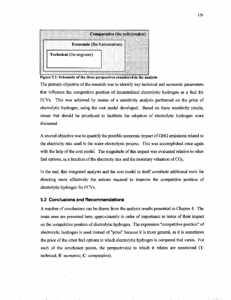
Figure 5.1: Schematic of the three perspectives considered in the anal lysis
The primary objective of the research was to identifl key technical and economic parameters
that influence the competitive position of decentralized electrolytic hydrogen as a fuel for
FCVs. This was achieved by means of a sensitivity analysis performed on the price of
electrolytic hydrogen, using the cost model developed. Based on these sensitivity results,
issues that should be prioritized to facilitate the adoption of electrolytic hydrogen were
discussed.
A second objective was to quantifl the possible economic impact of GHG emissions related to
the electricity mix used in the water electrolysis process. This was accomplished once again
with the help of the cost model. The magnitude of this impact was evaluated relative to other
fuel options, as a function of the electricity mix and the monetary valuation of C02.
In the end, Ulls integrated analysis and the cost model in itself constitute additional tools for
directing more effectively the actions required to improve the competitive position of
electrolyhc hydrogen for FCVs.
5.2 Conclusions and Recommendations
A number of conclusions can be drawn fi-om the analysis results presented in Chapter 4. The
main ones are presented here, approximately in order of importance in terms of their impact
on the competitive position of electrolyhc hydrogen. The expression "competitive position" of
electrolyhc hydrogen is used instead of "price" because it is more general, as it is sometimes
the price of the other fuel options to which electrolytic hydrogen is compared that varies. For
each of the conclusion points, the perspective(s) to which it relates are mentioned (T:
techcal, E: economic, C: comparative).

1 . The technical aspect is not the dominant one afecting the competitive position of
electrolytic hydrogen. (T, E, C )
In fact, the analysis showed that some issues in both of the economic and comparative
perspectives rank hgher in terms of impact on electrolytic hydrogen than the highest issue
in the technical perspective (storage). This suggests that the technical aspect has, in
general, the lowest impact of the three perspectives considered.
Efforts should therefore be focused primarily on electricity prices and taxeslcredits to
maximize the competitive position of electrolyhc hydrogen. l h s is an important result,
especially for engineers, who are used to solving problems largely fiom a technical
perspective. It means that even the best technical improvements, although helpful in
enhancing the competitiveness of electrolytic hydrogen, are unlikely to produce a decisive
advantage.
2. Strategies for low-cost electricity are key for electrolytic hydrogen to be competitive with
otherfiel options. (E)
Access to low-cost electricity remains the number one issue affecting the price of
electrolytic hydrogen. Three specific avenues were identified to achieve this goal:
Optimizing access to off-peak electricity by establishing new tariff structures better
adapted for off-peak electricity.
Talung advantage of the interruptible nature of water electrolysis to use spinning
reserves of power utilities at low rates, with limited additional GHG emissions.
Offering some fiscal incentives for electrolytic hydrogen produced fiom electricity
with low associated GHG emissions. Recall fiom the analysis portion that the price of
electrolytic hydrogen can be thought of in general as proportional to the electricity
price plus 1-3 #/kWh for capital and O&M costs. Hence a credit in the order of 1-3
#/kWh would have an impact comparable to lowering the capital cost of the
electrolyzer station to zero.
3. Site-specijic factors have an important impact on electrolytic hydrogen, particularly taxes
and credits onfiels. (C)

Analysis of the competitive position of electrolyhc hydrogen versus gasoline in three
locations (Vancouver, Los Angeles and Paris) showed that hydrogen could be sold at a
price comparable to or lower than gasoline (per kilometer) for two of these cities. This
assertion is based on actual local electricity rates and gasoline prices, and it holds true even
when electrolytic hydrogen is taxed at the same rate as gasoline on an energy content
basis.
It is shown that it would be possible today for electrolytic hydrogen to compete with
gasoline under favorable conditions of electricity prices and fbel taxes. Taxing fbels on an
energy content basis creates an incentive for more efficient fbel options. Fuel economy
improvements in ICE vehicles, like those achievable with hybrid cars, would make it
harder for electrolytic hydrogen to compete, but not dramatically so.
Other site-specific factors that can influence the price of electrolytic hydrogen, albeit to a
lesser extent, include the economic parameters used for the financing of the electrolyzer
station and the local electricity mix.
4. Storage of hydrogen seems to be the dominant technical issue. (T)
This is a surprising result, but the capital cost of hydrogen storage to allow the "fast fill"
option turns out to be of the same order or higher than the cost of the electrolyzer and
compressor components combined. This is emphasized in very small electrolyzer stations.
Approaches suggested in the analysis to remedy this situation include:
Eliminating the requirements for stationary hydrogen storage by making the "time fill"
option acceptable. One particularly ambitious approach is to have a small electrolyzer
directly onboard FCVs, to produce hydrogen wherever the FCV can be connected to
the electric grid, provided there exists a convenient way to bill th~s electricity to the
user.
Using a compressor to optimize the fraction of stored hydrogen that can be transfmed
to the high-pressure tanks of the FCV. This compressor could be the same as the one
used for compressing the stored hydrogen in the first place.
Developing inexpensive hydrogen storage technology.

5. Power utilities are in the best position tojnance & manage electrolyzer stations. (E)
A utility can generally afford a lower expected rate of return than a business on
electrolyzer stations, because its main financial interest comes fiom additional sales of
electricity. Also, utilities themselves usually have access to low-cost financing.
A utility could offer the flexibility that is necessary to adapt to an evolving market for
electrolyhc hydrogen. As the demand increases, a utility could replace small electrolyzers
by larger ones and move the smaller ones to locations with lower demand. Electrolyzer
stations of proper capacity would then be amortized over their 111 economic life, and their
capital cost could be averaged, the most profitable stations compensating for the ones with
a lower utilization.
Using communication technology, utilities could manage distributed electrolyzers as
"recallable" loads (i.e. power supplies that can be interrupted when needed), hence
promoting access to very low-cost electricity.
6. The monetary valuation of GHG emissions is generally not suficient to tilt the balance in
favor of electrolytic hydrogen. (C)
Even at US $20/ton of C02, the economic advantage of C02-fiee electrolytic hydrogen
with respect to gasoline used in ICE vehcles would be moderate. It would have an impact
equivalent to a credit of 1.1 $/kWh on electricity. This potential advantage of C02-free
electrolytic hydrogen vanishes almost completely when compared to hydrogen fiom
decentralized SMR, the maximum impact being equivalent to a credit of 0.4 $/kWh on
electricity.
Also, the electricity mix in most locations results in hgher GHG emissions than
decentralized SMR. For the electricity mix to produce lower GHG emissions than
decentralized SMR, at most 35% of the mix can come fiom natural gas power plants and
the rest fiom C02-fi-ee electricity. The use of electricity fiom spinning reserves could be
an exception, considering that most of the associated GHG emissions would be produced
regardless, for network reliability purposes.

7. A decentralized hydrogen fie1 infi.astructure may be better adapted to an emerging
market, but there are non-negligible disadvantages to very small stations. (T, E )
The size of a hydrogen fbelling station has an effect on its requirements to deal with
statistical variations in demand. The smaller the station, the greater the statistical
variations, and consequently the requirements to deal with them. These requirements are
handled primarily by the storage capacity, but also partially by the electrolyzer and
compressor, based on a hgher peak-to-demand ratio for smaller stations. In addition,
larger electrolyzers could often benefit fiom lower electricity prices.
This suggests that electrolyzer stations supporting a larger fleet of FCVs (say 50-100
instead of 2-4) could best serve the advantages of a decentralized hydrogen fuelling
infrastructure.
8. Technical issues related to the electrolyzer itselfhave a limited impact on the competitive
position of electrolytic hydrogen. (T)
The operating conditions of the electrolyzer (temperature, pressure, current density) and its
energy efficiency can all have positive effects on the performance and capital cost of the
electrolyzer, but their overall effect on the price of electrolytic hydrogen is moderate. The
most promising development on that fiont is probably the potential use of inexpensive
heat in high-temperature electrolysis (HTE), which could reduce the electricity
requirement by up to 25%.
The volume of electrolyzer stations manufactured shows a bigger impact on the cost of
electrolytic hydrogen than most other technical improvements.
9. The economic impact of the compression issue is also limited (T)
Improvements in that area, like the elimination of the compressor by high-pressure
electrolysis, would have more impact fiom an operational standpoint, whereas its impact
on the price of hydrogen would be rather modest. If very high-pressure hydrogen storage
(700 bar) becomes a standard, the impact of the compression issue could be slightly more
important.

10. The synergy with fie1 cell developments and production volumes could have a noticeable
impact on the capital cost of electrolyzers. However, synergies with &el cells could end
up favoring decentralized SMR more than water electrolysis.
Since the commercialization of stationary fuel cell systems is anticipated to take off prior
to any mass market in transportation, and natural gas is the clear dominant fuel option for
these stationary systems, small-scale SMR is expected to be well developed in the near
future.
The fuel processor in a stationary fuel cell system (likely based on small-scale SMR)
could be slightly oversized to produce excess hydrogen during off-peak periods. This
hydrogen could be stored for use in FCVs. Wherever natural gas is available, having a
fuel processor that serves a dual role, taking advantage of off-peak periods, could be a
more economical option than electrolytic hydrogen.
As a reminder, the reader should bear in mind that all these conclusions about the competitive
position of electrolytic hydrogen as a fuel for FCVs are based on a comparison of fuel costs
only, independently of the capital and operating costs of the vehicle. In reality, for FCVs to
compete with ICE vehicles on an economic basis, it is the life-cycle costs of owning and
operating the vehcle that must be similar. Fuel costs typically account for less than 10% of
the total cost of owning and operating a car. However, given the hgh sensitivity of consumers
to fuel costs, consumer behavior in itself justifies the comparison of fuel costs separately.
The overall conclusion that emerges fi-om this study is that electrolytic hydrogen could be
competitive with gasoline today, with current electrolysis technology, in locations where
electricity rates are low and/or fuel taxes are high. At the end of the day, there is no clear-cut
answer to whether decentralized electrolytic hydrogen is the best fuelling option for FCV.
The only certain answer is that it depends on a variety of issues pertaining to multiple
perspectives.
5.3 Future Work
This research covered a wide range of topics associated with decentralized electrolyhc
hydrogen as a fuel for FCVs, and was consequently limited in depth. More focused research

should follow on some of the issues raised here. Various studies have already been done and
published since h s research was initially started, but much remains to be done. A few
directions for future work are suggested:
Identify the most favorable locations, nationally or internationally for decentralized
electrolytic hydrogen stations. These could be locations where electricity price are low
compared to natural gas, where the electricity mix has low GHG emissions, where fuel
taxes are high, etc. More attention should be paid to comparing specifically hydrogen
fiom decentralized electrolysis with hydrogen fiom decentralized SMR.
Investigate the optimal strategies to supply low-cost electricity for the production of
electrolytic hydrogen.
Investigate the technical and economic implications of onboard electrolysis for FCVs.
Perform a rigorous study of the available tax and credit strategies to maximize the
competitive position of electrolyhc hydrogen.

References
- -- --
1. Van Vorst WM.D., George R.S. "Impact of the California Clean Air Act". International Journal of Hydrogen Energy 1997; 22 (1): 3 1-38.
2. PricewaterhouseCoopers and Fuel Cells Canada. Fuel Cells: The Opportunitv for Canada. June, 2002,72 p.
3. Mao Z. "The Development of Hydrogen Energy in China". In: Proceedings of the 1 4 ~ World Hydrogen Energy Conference, Montreal, Canada, 9-1 3 June 2002.
4. Thomas C.E., James B.D., Lomax F.D. Jr, Kuhn I.F. Jr. "Fuel Options for the Fuel Cell Vehicle: Hydrogen, Methanol or Gasoline?" International Journal of Hydrogen Energy 25 (2000): 551-567.
5. Pernbina Institute for Appropriate Development, Climate-Friendly Hvdronen Fuel: A Comparison of the Life-cycle Greenhouse Gas Emissions for Selected Fuel Cell Vehcle Hydrogen Production Systems. Report written with support fiom The David Suzuki Foundation, March 2000,44 p.
6. Fairlie M.J., Scott P.B. "Filling up with Hydrogen 2000". In: Proceedings of the 1999 US Department of Energy Hydrogen Program Review. Document No. NREUCP-570-26938, 1999.
7. Norsk Hydro web site: www.electrol~sers.com
8. Ballard Power Systems web site: www.ballard.com
9. Cropper M. "Fuel Cell Market Survey: Light Duty Vehicles". In: Fuel Cell Today web site www. fuelcelltoday.com. 1 5 January, 2003.
10. Cropper M. "Fuel Cell Market Survey: Buses". Fuel Cell Today web site www.fuelcelltoday.com. 26 November, 2003.
1 1. General Motors web site: www.gm.com
12. California Fuel Cell Partnership web site: www.fuelcellpartnershp.org
13. Lee H. "California Makes Plan to Fuel up on Hydrogen". In: Fuel Cell Today web site www.fue'lcelltoday.com. 3 February, 2004.
14. DderChrysler web site: www.daim1erchrysler.com
15. The Center for Global Studies. The Clean Development Mechanism: A Canadian Perspective. University of Victoria, Victoria, Canada, 2000.46 p.

- -
16. Intergovernmental Panel on Climate Change. Climate Chawe 2001 : The Scientific Basis. Houghton J.I., Ding Y ., D.J. Griggs, Noguer M., van der Linden P.J., Xiaosu D. (Eds.), Cambridge University Press, UK. 944 p.
17. Miller A.I., Duffey R.B. Constraining Climate Change with Nuclear Electricitv and Hvdrogen RJ + H2). Report No. AECL-12142, Atomic Energy of Canada Limited, Chalk River, Canada, 2003.46 p.
18. Intergovernmental Panel on Climate Change. Climate Change 2001 : Impacts, Adaptation & Vulnerabilitv. McCarthy J.J., Canziani O.F., Leary N.A., Dokken D. J., White K.S. (Eds.), Cambridge University Press, UK. 1000 p.
19. National Round Table on the Environment and the Economy. Greenhouse Gas Emissions from Urban Transportation: Backgrounder. Ottawa, Canada, 1998.
20. C02e web site: www.co2e.com
2 1. Gaudernack B. "Hydrogen Production from Fossil Fuels". In: Hydrogen Power: Theoretical and Engineering Solutions, Proceedings of the HYPOTHESIS I1 Symposium, Grimstad, Norway, 18-22 August, 1997. Kluwer Academic Publishers, the Netherlands, 1998,75-89.
22. Andreass? K., "Hydrogen Production by Electrolysis". In: Hydrogen Power: Theoretical and Engineering Solutions, Proceedings of the HYPOTHESIS I1 Symposium, Grimstad, Norway, 1 8-22 August, 1997. Kluwer Academic Publishers, the Netherlands, 1998,9 1 - 102.
23. Tilak B.V., Lu P.W.T., Colman J.E. and Srinivasan S., Electrolytic Production of Hydrogen, Chap. 1 of Comprehensive Treatise of Electrochemistrv, Vol. 2: Electrochemical Processing, J. Bockris, B. E. Conway, E. Yeager and R. E. White eds. Plenum Press, New York, 198 1.
24. Hox K, Lynum S. "More Efficient, Economical and Environmentally Friendly Utilisation of Natural Gas - How to Produce Hydrogen and Not C02". In: Hydrogen Power: Theoretical and Engineering Solutions, Proceedings of the HYPOTHESIS I1 Symposium, Grimstad, Norway, 1 8-22 August, 1997, Kluwer Academic Publishers, the Netherlands, 1998.
25. ZECA Corporation web site: www.zeca.org
26. Yoshida K. "UT-3 Thennochemical Hydrogen Production Process Driven by Conventional Heat Sources". In: Proceedings of the 12' world Hydrogen Energy Conference, Buenos Aires, Argentina, 1998,807-8 1 6.
27. U.S. Department of Energy. FY 2003 Promess R w r t for Hydrogen, Fuel Cells and Infrastructure Technolonies P r o m . Approved by Steven Chalk, October, 2003.

28. Padro C.E.G., Putsche V. Survey of the Economics of Hydrogen Technologies, NICH Report No. TP-570-27079, National Renewable Energy Laboratory, Colorado, U.S., 1999, 57 p.
29. Ogden J.M. "Prospects for Building a Hydrogen Energy Infrastructure". In Annual Review of Energy and the Environment, 1999,24: 227-279.
30. General Motors and Argonne National Laboratory. Well-to-Wheel E n e w Use and Greenhouse Gas Emissions of Advanced FueWehicle Systems - North American Analysis. June, 200 1.
3 1. California Fuel Cell Partnership. Bringing Fuel Cell Vehicles to Market: Scenarios and Challenges with Fuel Alternatives. Prepared for the California Fuel Cell Partnership by Bevilacqua Knight Inc., October, 2001.
32. Hamrnerli M., Stuart A. "Build-up of a Hydrogen Infrastructure". In: Proceedings of the ~onfaen'ce Fuel Cells 2000, Lucerne, Switzerland, 10-14 July 2000,339-348.
33. European Commission Directorate-General XI1 Science, Research and Development. ExternE Externalities of Enerm. Vol. 1 : Summary, compiled by ETSU, UK, 1996.
34. Hammerli M. "When Will Electrolyhc Hydrogen Production Become Competitive?" International Journal of Hydrogen Energy 1984; 9 (112): 25-51
3 5. Hassmann K., Khune H. "Primary Energy Sources for Hydrogen Production". In: Proceedings of the 9h World Hydrogen Energy Conference, Paris, France, 22-25 June 1992,1967-1 973.
36. Scott D.S. "The Energy System". International Journal of Hydrogen Energy 1994; 19 (6).
37. Thomas C.E., James B.D., Lomax F.D. Jr, Kuhn I.F. Jr. "Fuel Infrastructure Costs for Fuel Cell Vehicles". In: Proceedings of the 9h Canadian Hydrogen Conference, Vancouver, Canada, 7-1 0 February 1999,452-462.
3 8. Directed Technologies Inc. web site: www. directedtechnolo!izies. corn
3 9. HzGen web site: www. h2gen. corn
40. Ogden J.M. "Developing an Infrastructure for Hydrogen Vehicles: a Southern California Case Study". International Journal of Hydrogen Energy 24 (1999): 709-730.
41. Natural Resources Canada. An Economic Analysis of Various Hvdrogen Fuelling Pathways from a Canadian Perspective. Prepared for Natural Resources Canada by the Tax Policy Services Group of Ernst & Young, October, 2003,98 p.
42. Fairlie M. FCV Fuel Supply Infrastructure: The Electrolysis Option, Electrolyser, Ltd. Toronto, Canada, December, 1996,105 p.

43. Thomas C.E., Kuhn I.F. Jr. Electrolyhc Hydrogen Production Infrastructure Options and Evaluation. Prepared for the National Renewable Energy Laboratory by Directed Technologies Inc. Report No. NRELSTP-463-7903, National Renewable Energy Laboratory, Colorado, U.S., 1995,51 p.
44. Mann M.K, Spath P.L., Amos W.A. "Technoeconomic Analysis of Different Options for the Production of Hydrogen fiom Sunlight, Wind, and Biomass". In: Proceedings of the Department of Energy Hydrogen Program Review Meeting, Alexandria, Virginia, 28-30 April, 1998.367-390.
45. Row J., Raynolds M., Woloshyniuk G. Life-Cycle Value Assessment (LCVA) of Fuel Supply Options for Fuel Cell Vehicles in Canada. Prepared for the Pembina Institute for Appropriate Development, June, 2002, 170 p.
46. Fuel Cells Canada. Hydrogen Pathways Greenhouse Gas Emissions and Energy Use. Prepared for Fuel Cells Canada by (s&T)~ Consultants Inc., December, 2003,56 p.
47. Louis J.J.J., "Well-To-Wheel Energy Use and Greenhouse Gas Emissions for Various Vehicle Technologies". SAE paper No. 2001 -01 -1 343, published by Society of Automotive Engineers, Inc., Warrendale, PA, U.S.A., 2001.
48. Norbeck J.M. et al. Hvdrogen Fuel for Surface Transportation, Chap. 4: Hydrogen Production. Published by Society of Automotive Engineers, Inc., Warrendale, PA, U.S.A., 1996.
49. Dicks A., Larminie J. Fuel Cell Systems Explained, lS' edition, John Wiley and Sons, 2000.
50. Yarnaguchi M., Shinohara T., Taniguchi H., Nakanori T., Okisawa K. "Development of 2500 an2 Solid Polymer Electrolyte Water Electrolyzer in WE-NET". In: Proceedings of the 12' International Conference on Hydrogen Energy, Buenos Aires, Argentina, 1998, 747-755.
5 1. New Energy and Industrial Technology Development Organization (NEDO). International Clean Energy Network Using Hydrogen Conversion WE-NET): 1998 Annual Summary Report on Results. March, 1999.135 p.
52. Schug C.A. "Operational Characteristics of High-pressure, High-Efficiency Water- Hydrogen-Electrolysis". International Journal of Hydrogen Energy 1998; 23 (1 2): 1 1 13- 1 120.
53. Schiller G., Heme R., Mohr P., Peinecke V. "High Performance Electrodes for an Advanced Intermittently Operated 10-kW Alkaline Water Electrolyzer". International Journal of Hydrogen Energy 1998; 23 (9): 761-765.

54. Mitlitsky F., Myers B., Weisberg A.H., Leonida A. "Applications and Developments of High Pressure PEM Systems". Presented at the Portable Fuel Cells Conference, Lucerne, Switzerland, 21 -24 June, 1999.
55. Dutta S., Block D.L., Port R.L. "Economic Assessment of Advanced Electrolyhc Hydrogen Production". International Journal of Hydrogen Energy 1990; 15 (6): 387-395.
56. Noyes Data Corporation. Hydrogen Manufacture by Electrolysis, Thermal Decomposition and Unusual Techniques. Edited by M.S. Casper, Park Ridge, NJ, U.S.A., 1978.
57. Dickson E.M. The Hvdrogen Enerw Economy. Praeger Publishers, New York, NY, U.S.A., 1977.
58. Rosen M.A., Scott D.S. "Exergy Analysis of Hydrogen Production fiom Heat and Water by Electrolysis". International Journal of Hydrogen Energy 1992; 17 (3): 199-204.
59. Rosen M.A. "Energy and Exergy Analyses of Electrolytic Hydrogen Production". International Journal of Hydrogen Energy 1995; 20 (7): 547-553.
60. Rosen M.A., Scott D.S. "Comparative Efficiency Assessments for a Range of Hydrogen Production Processes". International Journal of Hydrogen Energy 1998; 23 (8): 653-659.
6 1. Dutta S. "Technology Assessment of Advanced Electrolytic Hydrogen Production". International Journal of Hydrogen Energy 1990; 15 (6): 379-386.
62. Cheng H., Scott K., Ramshaw C. "Intensification of Water Electrolysis in a Centrifugal Field". Journal of The Electrochemical Society 2002; 149 (1 1): D172-D177.
63. Pham A. "High Efficiency Steam Electrolyzer". In: Proceedings of the 1999 U.S. Department of Energy Hydrogen Program Review, Report No. NREWCP-570-26938, 1999.
64. Forschungszentrum Julich. "High-pressure Electrolyser". Informational document published by Forschungszen~ Jiilich GmbH, Jiilich, Germany, 2001.
65. Fuel Cells Bulletin. "Four Teams in DOE Programme for Ultra-Low-Cost SOFC". In: Fuel Cells Bulletin (October 2001 issue), published by Elsevier, October, 2001.
66. Mitlitsky F., Myers B., Weisberg A.H. "Regenerative Fuel Cell Systems". Energy & Fuels 1998; 12: 56-71.
67. Milliken C.E., Ruhl R.C. "Low Cost, High Efficiency Reversible Fuel Cell Systems". In: Proceedings of the 2002 U.S. Department of Energy Hydrogen Program Review, Report NO. NRELICP-610-32405,2002.
68. Stuart Energy web site: www.stuartenerm.com

- -
69. MTU web site: www.mtu-friedrichshafen.com
70. Hamilton Sundstrand web site: www.hsssi.com
7 1. Proton Energy Systems web site: www.protonenerm.com
72. ~ ~ d r o ~ & c s web site: www.hydrogenics.com
73. Dones R., Gantner U., Hirschberg S. "Greenhouse Gas Total Emissions from Current and Future Energy and Heat Supply Systems". In: Proceedings of the 4th International Conference on Greenhouse Gas Control Technologies, Interlaken, Switzerland, 3 1 Aug.- 2 Sept. 1998, Pergamon, Amsterdam, 1999.891 -896.
74. International Atomic Energy Agency (IAEA). Electronic document obtained from personal communication with H,-H. Rogner from the IAEA in October 2000. IAEA, Vienna, Austria.
75. Kurtz M. Handbook of Engineering Economics. McGraw-Hill, New York, U.S.A., 1984.
76. Federation of Canadian Municipalities. Keating-Nause S. "Towards Sustainability Municipal Infrastructure and Water Efficiency". Forum, Winter 1999; 23 (112): 34.
77. U.S. Environmental Protection Agency web site: www.epa.gov
78. Monk R.J., Gurney J. "Sustainable Hydrogen by Wire BC Hydro's Hydrogen Strategy". 2001.
79. BC Hydro web site: www.bchydro.com
80. International Energy Agency (IEA), World Enem Outlook. 1998 Edition, W O E C D , Paris, France, 1999.

Appendix A - Thermodynamic Voltages
for Water Splitting
The cost model of this research calculates the energy requirement of the electrolysis process,
based on theoretical considerations fiom thermodynamics and the energy efficiency of the
process, the latter being an input variable in the model.
As explained in chapter 2, the energy requirement of water electrolysis is proportional to the
single-cell voltage (for a constant current efficiency). The minimum amount of energy
necessary in the form of electricity is proportional to the reversible voltage (L). The
minimum fkom electricity and heat combined is proportional to the thermoneutral voltage
( ) And if the energy necessary to bring the feed water fiom 25•‹C to the electrolysis
temperature is included, then the total energy requirement is proportional to the so-called
higher-heating-value voltage (EHHv). The value of these different voltages as a function of
temperature was summarized in a graph of chapter 2, reproduced below (figure A.l). This
appendix explains how each of these four theoretical voltage curves were obtained.
Temperature (K)
Figure A.l: Theoretical water electrolysis voltages as a function of temperature (at 1 bar).

The refaence voltage used in the model to calculate the theoretical minimum energy
requirement is the higher-heating-value voltage (Em) . This is a conservative assumption, as
it implies that none of the energy used to heat the feed water to the electrolyzer operating
temperature is recycled.
Numerical values for Em as a hct ion of temperature were obtained by applying the First
Law of Thermodynamics to a simplified version of the electrolysis process. The only reactant
entering the electrolyzer is pure liquid water at a temperature To = 298 K. Work (W) and heat
(Q) are then added in the electrolyzer to split water completely into hydrogen and oxygen, the
two productscorning out at the electrolyzer operating temperature T, as shown in figure A.2.
Figure A.2: Schematic of the simplified electrolysis process used to calculate the theoretical energy requirement of the process.
The First Law of Thermodynamics states that energy is conserved. When applied to a control
volume, it can be expressed in a general form as:
The rate of change of energy in the control volume (dE/dt) is equal to the sum of the net heat,
work and enthalpy flows into and from the control volume. Here, work done on the control
volume by its surrounding is considered positive, as well as the heat input to the control
volume.
At steady state, the left hand side of equation (A.l) becomes zero. The magnitude of the
combined heat and work input is then equal to the net enthalpy change between the products
(exiting the control volume) and reactants (entering the control volume). When the enthalpy
flows are expressed in mold terms, equation (A. 1) becomes:

Q+ ~=x l i , (h~+AL)~-x l i~ (h~ +AZ)~ ( A.2)
The subscripts "p" and "r" on the right hand side of equation (A.2) stand for products and
reactants. The enthalpy of each reactant or product can be expressed as the sum of its enthalpy
of formation (h; ) at STP ' conditions (as indicated by the " superscript), and the difference in
enthalpy between standard temperature (298.15 K) and the temperature T considered ( G ) .
The mold form of these quantities is indicated by a "bar" over the lower case letter.
If equation (A.2) is divided by the mold flow, it gives:
The water-splitting reaction considered here is simply:
When equation (A.3) is applied to the water-splitting reaction, the result is:
Considering that the enthalpy of formation of diatomic gases like molecular oxygen and -
hydrogen is equal to zero by convention, and that the " Ilh " of water is equal to zero because
taken at standard temperature 298.15 K, we find:
The enthalpy of formation of water at STP is a fixed value: h;,,, = -285.83 kllmol.
However, the enthalpy of hydrogen and oxygen must be calculated as a function of
temperature using some kind of relationship. For an ideal gas, the change in enthalpy between
two states can be calculated fiom the specific heat at constant pressure (C,) and the
temperature of each state, provided there is a relationship to express Cp as a function of
temperature. Applying this approach, equation (A.6) becomes:
' Standard temperature and pressure or standard reference state, i.e. 25 "C (298.15 K) and 1 bar.

Standard thermodynamics textbooks generally provide empirical relationships to calculate C,
as a function of temperature for common substances. In the cost model, the following
relationships were used to calculate the integrals of equation (A.7) for hydrogen and oxygen ':
- with: a = 3.057, P = 2.677xl0", y = 5.810~10", 6 = 5.521~10-~, 6 = 1.812~10-'~, R = 8.314 kJ/kmol.K
with: cl, = 3.626, Po = 1.878x1o4, yo = 7.055x10⁴, 6, = 6.764~10-~, E, = 2.156~10-l2
Thus, using these relationships it is possible to evaluate the theoretical amount of energy
(Q+W) required to split water as a function of temperature, and to heat the feed water fiom
25•‹C to the water-splitting temperature T. The corresponding higher-heating-value voltage
(Em) is obtained simply by dividing this minimum energy requirement (Q+W) by nF, where
n = 2 for the water-splitting reaction and F is the Faraday constant (96,487). Actual values
used in the model to calculate Em are presented in table A. 1.
The previous paragraphs explain how the values for Em (T) were obtained. For the purpose
of the cost model, Em is the most important voltage since it is the reference voltage used to
calculate the minimum energy requirement of the electrolyzer. However, the three other
voltage curves appearing in figure (A.l) also provide usell information. Their values were
obtained fiom a computer program that calculates various thermodynamic quantities, based on
the molecular properties of the species considered 2.
' M o m M.J., Shapiro H.N. Fundamentals of Engineering Thermodynamics. Third edition, John Wiley and Sons, 1998. Computer program developed by Dr. David Harrington, University of Victoria, Victoria, BC, Canada, 2000.

Table A.l: Values used to calculate the higher-heating-value voltage (Em) as a function of temperature.
Recall fiom Chapter 2 that the theoretical energy required for the water-splitting reaction to
proceed (ignoring the energy to heat the feed water to the electrolysis temperature), can be
expressed through the following thermodynamic equation:
AH=AG+TAS (A. 10)
where AH is the enthalpy change of the reaction, AG is the Gibbs flee energy change, T is the
electrolysis temperature (in Kelvin) and AS is the entropy change.
The Gibbs fiee energy change AG corresponds to the portion of the total reaction energy that
must be supplied in the form of electricity, when water splitting is performed by electrolysis.
The term "TAS" corresponds to the portion of the total reaction energy that could
thermodynamically be covered by thermal energy.

All the terms of equation (A.lO) can be divided by "2Ft (F is the Faraday constant) to give
respectively the thermoneutral voltage (Em), the reversible voltage (Em) and the voltage that
corresponds to the portion of energy which could theoretically be covered by heat (TASI2F).
AH AG TAS - +-
2 F 2 F 2 F
AG E =- rev 2 F
(A. 1 1)
(A. 12)
(A. 13)
Thus, calculating the values of AH and AG as a hc t ion of temperature, at standard pressure
of 1 bar, is sufficient to obtain the value of the three voltages mentioned above. These two
quantities were calculated respectively by taking the negative of the enthalpy of formation and
the negative of the Gibbs hc t ion of formation of water at temperature T. Hence the two
corresponding equations used to calculate the enthalpy change and Gibbs free energy change
for the water-splitting reaction are:
All the input values for these two equations were obtained fiom the computer program
referred to earlier ', and fiom tables of chemical thermodynamic properties 2.
The resulting values for AH(T) and AG(T) are then divided by 2F to give the corresponding
therrnoneutral (&) and reversible (GV) voltages. The voltage that corresponds to the portion
of energy which could theoretically be covered by heat (TASI2F) is simply obtained &om the
difference between & and E&, in accordance with equation (A.ll). All the voltage values
used to generate figure (A. 1) are summarized in table (A.2).
I Computer program developed by Dr. David Harrington, University of Victoria, Victoria, BC, Canada, 2000. National Bureau of Standards. The NSB Tables of Chemical Thermodynamic Properties. Journal of Physics and Chemical Reference Data, Vol. 1 1, 1982, Supplement No. 2.

Most standard thermodynamics textbooks provide the necessary information to reproduce
H20 liq.
H20 gas
these results. Some references also provide a more extensive treatment of the First and
Second Laws of Thermodynamics applied to water electrolysis 4.5.
T f"Cf 25 50 100 100 150 200 250
1 Calculated from the values obtained with the computer program developed by Dr. David Harrington. 2 Simply the difference between E, and &. 3 Calculated fiom application of First-Law of Thermodynamics, using empirical relationships for CpH2 and C.2. 4 Noyes Data Corporation. Hydrogen Manufacture by Electrolysis, Thermal Decornosition and Unusual
Techniques. Edited by M.S. Casper, Park Ridge, NJ, U.S.A., 1978 ' Winter C.J. Hydrogen as an Enerw Carrier - Technologies. Systems, Economv. Joachim Nitsch (Eds.),
Springer-Verlag, 1 988.
800 850 900 950 1000
T @l 298 323 373 373 423 473 523
Table A.2: Summary table of the relevant voltages used for the water-splitting reaction
1073 1123 1173 1223 1273
E,, = AH /2F 'I'
1,481 1,477 1,469 1,258 1,26 1 1,263 1 266
1,287 1,288 1,290 1,29 1 1,292
E,,, = AG 121; (I'
1,229 1,208 1,167 1,168 1,156 1,144 1 131
0,980 0,965 0,95 1 0,936 0,922
TASI2F G, 0,252 0,269 0,302 0,090 0,105 0,120 0 135
&im/ t3)
1,481 1,487 1,498 1,498 1,509 1,521 1 533
0,307 0,323 0,339 0,354 0,370
1,665 1,678 1,690 1,703 1,716

Appendix B - Fuel Economy
Conversions
To facilitate comparisons between the different fuel options considered in this research, their
respective he1 economies have all been expressed in terms of equivalent gasoline fuel
economy. This is a common practice in most studies comparing he1 options for FCVs.
When gasoline is the fuel considered, either in an ICE vehicle or a FCV, the average &el
consumption can be expressed directly in liters of gasoline per 100 lulometres (lilter1100 km)
or in miles per gallon (mpg) in the United States. When the fuel considered is methanol or
hydrogen however, their energy content has to be translated in a gasoline equivalent. This can
be done by comparing hels on a higher-heating-value (HHV) basis or on a lower-heating-
value basis (HHV). Some studies use the higher heating value (HHV), some use the lower
heating value' (LHV), and others do not specify which one is used.
The use of the LHV-basis can be justified by the fact that no vehicles in use or currently being
developed have power plants capable of condensing the moisture of combustion '. On the
other hand, the main argument for comparison on a HHV-basis is that it reflects more
accurately the true energy content of a fuel. In this research, fuel comparisons are all made on
a HHV-basis. The impact of using HHV instead of LHV is quantified for hydrogen and
methanol, as shown below.
A table fiom the Alternative Fuels Data Centre ' is the refaence used for the energy content of
gasoline and methanol, whereas a diffaent source is used for the energy content of hydrogen2.
Energy content of gasoline:
I Alternative Fuels Data Centre web site: www.afdc.doe.~ov/vdfs/fueltable.vdf , "Properties of Fuels" table. 2 Norbeck J.M. et al. Hvdronen Fuel for Surface Transportation. Published by Society of Automotive Engineers,
Inc., Warrendale, PA, U.S.A., 1996.

13 1,670 kJ/gallon (HHV) / 3.7854 galloditre = 34,784 kJAiter of gasoline (HHV) 121,330 kJIgallon (LHV) I 3.7854 galloditre = 32,052 kJ/liter of gasoline (LHV)
Energy content of methanol:
68,156 ldgallon (HHV) / 3.7854 gallonflitre = 18,005 kJlliter of methanol 0 59,947 Wlgallon (LHV) / 3.7854 gallonflitre = 15,836 kT/liter of methanol (LHV)
Energy content of hydrogen:
14 1,860 kJkg of hydrogen (HHV) 1 19,930 kJkg of hydrogen (LHV)
Example of fuel economy conversions with the base case values used in the cost model:
The base case fuel economy of the gasoline ICE vehicle is 7.30 liter1100 km. In terms of the
energy requirement to drive 100 kilometers, it means:
7.30 liter1100 km * 34,784 kT/liter of gasoline (HHV) = 253,923 kT/ 100 km (HHV)
7.30 liter1100 km * 32,052 WAiter of gasoline (LHV) = 233,980 kJ/ 100 km (LHV)
The base case fuel economy of the methanol FCV is 4.19 liter11 00 km, in gasoline equivalent.
l h s value is the same as the one used in the Pembina Institute's report ' . Assuming this value
is taken as the gasoline equivalent of methanol (MeOH) on a HHV-basis, it means that the
energy requirement to drive 100 kilometers is:
4.19 liter 11 00 krn * 34,784 Wlliter of gasoline (HHV) = 145,745 W 100 km (HHV)
or in terms of actual methanol consumption:
[145,745 kJ1100 km] / [l8,OO5 kT/liter MeOH (HHV)] = 8.09 litre MeOW 100 km
If the same fuel economy value of 4.19 liter1100 km is taken as the gasoline equivalent of
methanol, but on a LHV-basis instead, the energy requirement to drive 100 kilometers is then:
4.19 liter 11 00 lun * 32,052 kJAiter of gasoline (LHV) = 134,298 W 100 km (LHV)
or in terms of actual methanol consumption:
[134,298 kT/ 100 km] 1 [15,836 kJAiter MeOH (LHV)] = 8.48 litre MeOHI 100 km
1 Pembina Institute for Appropriate Development, Climate-Friendly Hydrogen Fuel: A Comparison of the Life- cycle Greenhouse Gas Emissions for Selected Fuel Cell Vehicle Hydrogen Production Systems. Report written with support fiom The David Suzuki Foundation, March 2000,44 p.

So the same he1 economy value of 4.19 liter11 00 krn (in gasoline equivalent) translates in a
slightly higher methanol consumption (about 4.8%) when gasoline and methanol are
compared on a LHV-basis instead of HHV-basis. Thus, by assuming that the he1 economy
value for methanol is given on a HHV instead of LHV-basis in the reference source l , the
model may be underestimating methanol consumption by about 5%.
The base case fuel economy of the hydrogen FCV is 3.02 liter1100 km, in gasoline equivalent.
Assuming this value is taken as the gasoline equivalent of hydrogen (H2) on a HHV-basis, it
means that the energy requirement to drive 100 kilometers is:
3.02 liter11 00 km * 34,784 mi te r of gasoline (HHV) = 105,048 W 100 km (HHV)
or in terms of actual hydrogen consumption:
[105,048 WlOOkm] 1 [l41,86O kJkg H2 (HHV)] = 0.741 kg H21100km -4 If the same fuel economy value of 3.02 liter1100 km is taken as the gasoline equivalent of
hydrogen, but on a LHV-basis instead, the energy requirement to drive 100 kilometers is then:
3.02 literA00 km * 32,052 kJlliter of gasoline (LHV) = 96,797 kT/ 100 km (LHV)
or in terms of actual hydrogen consumption:
[96,797 WlOOkm] 1 [119,930 klkg H2 (LHV)] = 0.807 kg HzIlOOkm -4 Hence, the same fuel economy value of 3.02 liter1100 km translates in a higher hydrogen
consumption (about 9%) when gasoline and hydrogen are compared on a LHV-basis instead
of HHV-basis. However, the base case value of 3.02 liter11 00 km (HHV) used in the model is
approximately 8% higher than the value used in the reference source (2.79 lited100 km) '. The net result is that the base case hydrogen consumption (135 kmkg H2) is nearly the same
as the one used in the reference source (1 34 kmlkg H2), assuming they used the LHV-basis to
express the "gasoline-equivalent" fuel economy of the hydrogen FCV.
To summarize, assuming that fuel comparisons are made on a HHV-basis rather than LHV-
basis may favor methanol by about 5% and hydrogen by 9%, when gasoline is the refaence
fuel.
1 Pembina Institute for Appropriate Development, Climate-Friendly Hydrogen Fuel: A Cowarison of the Life- cvcle Greenhouse Gas Emissions for Selected Fuel Cell Vehicle Hvdrogen Production Svstems. Report written with support fiom The David Suzuki Foundation, March 2000,44 p.

149
Appendix C - Cost Model Developed in
Microsoft Excel
The following is a print out of the actual cost model developed in Excel 2000. It consists of
six worksheets, of which the most relevant sections are printed here.
They include, in the order presented:
- 7 pages fi-om the Input Summary worksheet
- 4 pages fi-om the Total Cost worksheet
- 3 pages fiom the Capital + O M Cost worksheet
- 2 pages fi-om the Energy Cost worksheet
- 2 pages fiom the GHG Cost or Saving worksheet
- 3 pages fiom the Site-Specific Information worksheet
The cost model includes a total of 103 interactive input cells. More than half are of these input
cells are related to other he1 options beside electrolytic hydrogen, and site-specific
information.

To
faci
litat
e th
e un
ders
tand
ing
of t
he v
ario
us v
alue
s di
spla
yed
in th
is m
odel
, a
code
of
colo
rs h
as b
een
used
.
Yel
low
cel
ls id
entif
y in
tera
ctiv
e in
put c
ells
.
Gre
en c
ells
are
non
-inte
ract
ive
cells
that
sim
ply
sum
mar
ize
(in
the
"Inp
ut S
umm
ary"
wor
kshe
et)
the
valu
es e
nter
ed in
all
the
yello
w c
ells
of t
he m
odel
.
Blu
e ce
lls id
entif
y th
e m
ain
outp
ut c
ells
of t
he m
odel
.
Ora
nge
cells
iden
tify
non-
inte
ract
ive
inpu
t cel
ls to
the
mod
el, i
n th
e se
nse
that
thei
r in
form
atio
n co
nten
t can
be
used
as
refe
renc
e fo
r in
tera
ctiv
e in
put,
but t
hey
are
not d
irect
ly li
nked
to a
ny o
ther
cel
ls.

1) N
eed
for
Hyd
rog
en F
uel
2) V
aria
ble
s In
fluen
cin
g C
apita
l + O
&M
Cos
t
Var
iabl
e U
nits
V
alue
Rd
Rat
io o
f pe
ak H
2 pr
oduc
tion
to a
vera
ge d
eman
d
f C
apac
ity fa
ctor
(av
erag
e us
e [h
ours
per
day
] 124
h)
e,
Uni
t cos
t of
elec
troly
zer p
er k
W,
cU
Uni
t cos
t of c
ompr
esso
r per
kW
Out
of H
2 (H
HV
)
D
Equ
ival
ent n
umbe
r of
days
of s
tora
ge
A
Ava
ilabl
e fr
actio
n of
sto
red
hydr
ogen
Su
S
tora
ge c
apita
l cos
t per
kg
of s
tore
d H
2 (H
HV
)
x C
apita
l cos
t of
bala
nce
of p
lant
V
Num
ber o
f veh
icle
s se
wed
by
stat
ion
M
Ave
rage
ann
ual m
ileag
e pe
r veh
icle
fe
Ave
rage
fuel
eco
nom
y
kmly
r km
lkg
H2
Var
iab
les
Invo
lved
in F
inan
cin
g th
e E
lect
roly
sis
Sta
tion
If
trea
ted
as a
hom
e ap
plia
nce,
ent
er 1
100
1920
0 13
5
i, M
ortg
age
inte
rest
rat
e (if
fina
nced
as
an a
pplia
nce)
T,
Per
sona
l tax
rat
e of
hom
e ow
ner
Gen
eral
infla
tion
rate
r A
fter-
tax
real
rate
of
retu
rn o
n in
vest
men
t (in
con
stan
t dol
lars
)
for
hom
e ap
plia
nce
case
for
hom
e ap
plia
nce
case
for
busi
ness
cas
e
for
busi
ness
cas
e
for
busi
ness
cas
e

Ixtr
aord
inar
y ex
pen
ses
El
extr
aord
inar
y ex
pens
e 1
n,
year
in w
hich
ext
raor
dina
ry e
xpen
se 1
occ
urs
En
extra
ordi
nary
exp
ense
2
n2
year
in
whi
ch e
xtra
ordi
nary
exp
ense
2 o
ccur
s
EB
extra
ordi
nary
exp
ense
3
n3
year
in
whi
ch e
xtra
ordi
nary
exp
ense
3 o
ccur
s
E4
extr
aord
inar
y ex
pens
e 4
n4
year
in w
hich
ext
raor
dina
ry e
xpen
se 4
occ
urs
E5
extra
ordi
nary
exp
ense
5
n5
year
in w
hich
ext
raor
dina
ry e
xpen
se 5
occ
urs
Ann
ual i
nsur
an
3) V
aria
ble
s In
fluen
cin
g E
nerg
y C
ost
as a
per
cent
age
of t
he to
tal
inst
alle
d ca
pita
l cos
t of t
he
elec
trol
ytic
hyd
roge
n re
fuel
ling
stat
ion
Tl,
Ene
rgy
effic
ienc
y of
ele
ctro
lyze
r
{Ene
rgy
inpu
t e- +
NG
(HH
V)}
q,
Com
pres
sor e
ffici
ency
(with
resp
ect t
o ad
iaba
tic c
ompr
essi
on)
P,-
Ele
ctric
ity p
rice
PNG
N
atur
al g
as p
rice
a
Fra
ctio
n of
ene
rgy
requ
ired
for
elec
trol
ysis
pro
vide
d by
NG
T
Ele
ctro
lysi
s tem
pera
ture
Pi
Ele
ctro
lysi
s pre
ssur
e
(als
o in
let p
ress
ure
to c
ompr
esso
r)
Po
O
utle
t pre
ssur
e fro
m c
ompr
esso
r
(als
o hy
drog
en s
tora
ge p
ress
ure)
Yo
Yo
$/kw
h $/
G J
"C
bar
bar

4) V
aria
ble
s In
fluen
cin
g th
e G
reen
ho
use
Gas
"A
dd
ed C
ost
ISav
ing
" C
om
po
nen
t
Tre
atm
ent
of C
GH
G (add
ed c
ost(
+)
or s
avin
g (-
) du
e to
GH
G e
valu
atio
n)
To e
xclu
de th
e im
pact
of
CG
HG
, on th
e un
it co
st o
f H
2 (U
) T
o in
clud
e C
G~
~
cons
ider
ing
the
alte
rnat
ive
optio
n:
Mo
net
ary
Eva
luat
ion
of
Gre
enh
ou
se G
as E
mis
sio
ns
) E
c02
I~va
lua
tio
n of C
02
equ
ival
ent e
mis
sion
s I U
S$/
ton
C0
21
20
1 0
ente
r 0
Gas
olin
e IC
E,
Gas
olin
e FC
V w
ith o
n-bo
ard
refo
rmin
g,
Met
hano
l FC
V w
ith o
n-bo
ard
refo
rmin
g,
Hyd
roge
n FC
V fr
om d
ecen
tral
ized
SM
R,
ente
r 1
ente
r 2
ente
r 3
ente
r 4
Bas
e C
ase
for
Eac
h O
ther
Fu
el O
ptio
n
Opt
ion
GH
G e
mis
sion
s lit
er o
f ga
solin
e 1
Fu
el E
cono
my
of O
ther
Fu
el O
ptio
ns
Opt
ion
Gas
olin
e IC
E
Gas
olin
e F
CV
on-
boar
d re
form
ing
Met
hano
l FC
V o
n-bo
ard
refo
rmin
g
Hyd
roge
n FC
V fr
om d
ecen
traliz
ed S
MR
liter
of g
asol
ine
equi
v. (
HH
V) p
er 1
00 k
m 4.
19
3.02
Gas
olin
e IC
E
Gas
olin
e FC
V o
n-bo
ard
refo
rmin
g
Met
hano
l FC
V o
n-bo
ard
refo
rmin
g
Hyd
roge
n FC
V fr
om d
ecen
traliz
ed S
MR
g (C
O2 ,,,, )Ik
m d
riven
248
193
162
80
equi
v. (H
HV
) per
100
km
7.30
6.
1 1
4.19
2.
79

Lo
catio
n
I ~a
nc
ou
ve
r I I
For V
anco
uver
, C
anad
a, e
nter
1
Fo
r Lo
s A
ngel
es,U
SA
, ent
er 2
Fo
r P
aris
, Fra
nce,
ent
er 3
Fo
r ano
ther
loca
tion
ente
r 4
5) S
ite-S
pec
ific
Info
rmat
ion
Aff
ectin
g C
om
par
iso
n w
ith O
ther
Fu
ellin
g O
ptio
ns
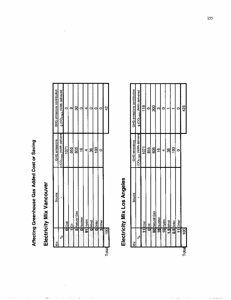
Aff
ectin
g G
reen
ho
use
Gas
Add
ed C
ost o
r S
avin
g
Ele
ctri
city
Mix
Van
couv
er
L~
ix
I S
ourc
e I
GH
G e
mis
sion
s I
GH
G e
mis
sion
s co
ntrib
utio
n I
%
0
Ele
ctri
city
Mix
Lo
s A
ngel
es
1 5 0
-,
Q1 0 0.
Mix
I
Sou
rce
I G
HG
em
issi
ons
I G
HG
em
issi
ons
cont
ribut
ion
Coa
l
oil
Nat
ural
Gas
Nuc
lear
Hyd
ro
Win
d
Sol
ar
I 85
5 I
0 ~
I~
at
ur
al
Gas
60
5 30
3
(CO
z eq
ulv )/
kwh
del
iver
e
1071
%
(Co
n eq
uw )
/kw
h d
eliv
ere
1071
16 N
ucle
ar
16
I 3
10 H
ydro
4
0 i
g (C
02
,,,,, )/
kwh
del
iver
ed
0 85
5 60
5 16
4 36
1 9
3
g (C
on
equw
)/k
wh
del
iver
ed
118 9
30
0 4 0 0
1.5
Win
d
Q.5
Sol
ar
11 O
ther
36
1 93 0
1 1 0
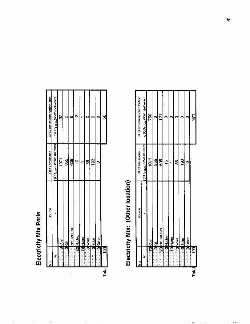
Ele
ctri
city
Mix
Par
is
l~
ix
I
Sou
rce
I G
HG
em
issi
ons
I G
HG
em
issi
ons
cont
ribut
ion
I Yo
3
Ele
ctri
city
Mix
: (O
ther
loca
tion
)
0 1
1
82
14
3
0
Mix
I
Sou
rce
I G
HG
em
issi
ons
I G
HG
em
issi
ons
cont
ribut
ion
Coa
l
oil
Nat
ural
Gas
Nuc
lear
Hyd
ro
Win
d
Sol
ar
(CO
P eq
ulv )/k
wh
deliv
ere
1071
YO 70
g (C
OP
equl
v )/
kwh
del
iver
ed
32
855
605
16
4 36
193
1 (CO
P ,,,, )
/kw
h de
liver
el
g (
C4
,,,, )
/kw
h d
eliv
ered
Coa
l I
1071
I 750 0 6 13
1 0 0
0 0
10
0
0
20 N
atur
al G
as
605
121
i
855
oil
0
Nuc
lear
Hyd
ro
Win
d
Sol
ar
16
4 36
193
0 0 0 0

To
tal C
ost
of
Ele
ctro
lytic
Hyd
roge
n
Var
iabl
e U
nits
V
alue
U
Uni
t cos
t of
H2
C
Tot
al a
nnua
l cos
t of
H2
Y
Ann
ual H
2 pr
oduc
tion
from
sta
tion
CC
A
nnua
l cap
ital a
nd O
&M
cos
t
Ce
A
nnua
l ene
rgy
cost
CG
HG
A
nnua
l add
ed c
ost(
+) o
r sa
ving
(-)
due
to G
HG
eva
luat
ion
2' C
= c
c + c
e (+C
GH
G)
**
Bec
ause
CG
HG
is a
rel
ativ
e te
rm d
epen
ding
on
the
alte
rnat
ive
optio
n co
nsid
ered
, it
is p
ossi
ble
to in
clud
e or
exc
lude
CG
HG
in th
e to
tal a
nnua
l cos
t of
H2
01
Com
pare
d to
: N
o co
rn p
aris
on
I -.
.-,
. .
I o
incl
ude
CG
HG
cons
ider
ing
the
alte
rnat
ive
optio
n:(
I T
reat
men
t of
CG
HG
I
To e
xclu
de
the
imp
act o
f C
GH
G. on
the
un
it co
st o
f H
2 (U
)
Gas
olin
e IC
E,
Gas
olin
e FC
V w
ith o
n-bo
ard
refo
rmin
g,
Met
han
ol F
CV
with
on
-bo
ard
refo
rmin
g,
Hyd
rog
en F
CV
from
dec
entr
aliz
ed S
MR
,
0 en
ter
0
ente
r 1
ente
r 2
ente
r 3
ente
r 4

4,
If ne
cess
ary,
the
requ
ired
annu
al h
ydro
gen
prod
uctio
n (Y
) cou
ld b
e ca
lcul
ated
usi
ng
the
spec
ific
mile
age
(Mi)
and
fuel
eco
nom
y ((
fJi)
of t
he v
ario
us v
ehic
les
to b
e
serv
ed b
y th
e st
atio
n:
5,
The
fuel
eco
nom
y of
a v
ehic
le (f,
), in
km
driv
en p
er k
g of
H2,
can
be
calc
ulat
ed:
A)
Dire
ctly
from
the
aver
age
ener
gy in
put r
equi
red
(HH
V)
per
km d
riven
fe [k
mlk
g H
2] =
ene
rgy
req
uir
ed (H
HV
) [k
J/km
] / 1
4 1,8
60 [k
J/kg
H2]
B) F
rom
the
equi
vale
nt fu
el e
cono
my
if ga
solin
e (H
HV
) wer
e us
ed,
eith
er in
equ
ival
ent l
iters
of g
asol
ine
per
100
km d
riven
fe [k
mlk
g H
2] =
407
.83
1 Lp
hkm
(u
sing
HH
V v
alue
s fo
r bo
th g
asol
ine
and
H2)
or in
mile
s pe
r U
S g
allo
n of
gas
olin
e eq
uiva
lent
(mpg
ge)
f, [k
mlk
g H
2] =
1.7
339
* m
pg
ge
(u
sing
HH
V v
alue
s fo
r bo
th g
asol
ine
and
H2)
Lphk
m: f
uel e
cono
my
in li
ters
of
gaso
line
equi
vale
nt (H
HV
) per
100
km
m
pgge
: fue
l eco
nom
y in
mile
s pe
r U
S g
allo
n of
gas
olin
e eq
uiva
lent
(HH
V)
For c
onsi
sten
ce in
this
res
earc
h, th
e hi
gher
-hea
ting-
valu
e is
alw
ays
the
one
used
for
gaso
line
met
hano
l and
hyd
roge
n w
hen
usin
g eq
uiva
lent
fuel
eco
nom
y.

Ele
ctri
city
Mix
Par
is
l~
ix
I
Sou
rce
I G
HG
em
issi
ons
I G
HG
em
issi
ons
cont
ribut
ion
I Yo
3
Ele
ctri
city
Mix
: (O
ther
loca
tion
)
0 1
1
82
14
3
0
Mix
I
Sou
rce
I G
HG
em
issi
ons
I G
HG
em
issi
ons
cont
ribut
ion
Coa
l
oil
Nat
ural
Gas
Nuc
lear
Hyd
ro
Win
d
Sol
ar
(CO
P eq
ulv )/k
wh
deliv
ere
1071
YO 70
g (C
OP
equl
v )/
kwh
del
iver
ed
32
855
605
16
4 36
193
1 (CO
P ,,,, )
/kw
h de
liver
el
g (
C4
,,,, )
/kw
h d
eliv
ered
Coa
l I
1071
I 750 0 6 13
1 0 0
0 0
10
0
0
20 N
atur
al G
as
605
121
i
855
oil
0
Nuc
lear
Hyd
ro
Win
d
Sol
ar
16
4 36
193
0 0 0 0

To
tal C
ost
of
Ele
ctro
lytic
Hyd
roge
n
Var
iabl
e U
nits
V
alue
U
Uni
t cos
t of
H2
C
Tot
al a
nnua
l cos
t of
H2
Y
Ann
ual H
2 pr
oduc
tion
from
sta
tion
CC
A
nnua
l cap
ital a
nd O
&M
cos
t
Ce
A
nnua
l ene
rgy
cost
CG
HG
A
nnua
l add
ed c
ost(
+) o
r sa
ving
(-)
due
to G
HG
eva
luat
ion
2' C
= c
c + c
e (+C
GH
G)
**
Bec
ause
CG
HG
is a
rel
ativ
e te
rm d
epen
ding
on
the
alte
rnat
ive
optio
n co
nsid
ered
, it
is p
ossi
ble
to in
clud
e or
exc
lude
CG
HG
in th
e to
tal a
nnua
l cos
t of
H2
01
Com
pare
d to
: N
o co
rn p
aris
on
I -.
.-,
. .
I o
incl
ude
CG
HG
cons
ider
ing
the
alte
rnat
ive
optio
n:(
I T
reat
men
t of
CG
HG
I
To e
xclu
de
the
imp
act o
f C
GH
G. on
the
un
it co
st o
f H
2 (U
)
Gas
olin
e IC
E,
Gas
olin
e FC
V w
ith o
n-bo
ard
refo
rmin
g,
Met
han
ol F
CV
with
on
-bo
ard
refo
rmin
g,
Hyd
rog
en F
CV
from
dec
entr
aliz
ed S
MR
,
0 en
ter
0
ente
r 1
ente
r 2
ente
r 3
ente
r 4

4,
If ne
cess
ary,
the
requ
ired
annu
al h
ydro
gen
prod
uctio
n (Y
) cou
ld b
e ca
lcul
ated
usi
ng
the
spec
ific
mile
age
(Mi)
and
fuel
eco
nom
y ((
fJi)
of t
he v
ario
us v
ehic
les
to b
e
serv
ed b
y th
e st
atio
n:
5,
The
fuel
eco
nom
y of
a v
ehic
le (f,
), in
km
driv
en p
er k
g of
H2,
can
be
calc
ulat
ed:
A)
Dire
ctly
from
the
aver
age
ener
gy in
put r
equi
red
(HH
V)
per
km d
riven
fe [k
mlk
g H
2] =
ene
rgy
req
uir
ed (H
HV
) [k
J/km
] / 1
4 1,8
60 [k
J/kg
H2]
B) F
rom
the
equi
vale
nt fu
el e
cono
my
if ga
solin
e (H
HV
) wer
e us
ed,
eith
er in
equ
ival
ent l
iters
of g
asol
ine
per
100
km d
riven
fe [k
mlk
g H
2] =
407
.83
1 Lp
hkm
(u
sing
HH
V v
alue
s fo
r bo
th g
asol
ine
and
H2)
or in
mile
s pe
r U
S g
allo
n of
gas
olin
e eq
uiva
lent
(mpg
ge)
f, [k
mlk
g H
2] =
1.7
339
* m
pg
ge
(u
sing
HH
V v
alue
s fo
r bo
th g
asol
ine
and
H2)
Lphk
m: f
uel e
cono
my
in li
ters
of
gaso
line
equi
vale
nt (H
HV
) per
100
km
m
pgge
: fue
l eco
nom
y in
mile
s pe
r U
S g
allo
n of
gas
olin
e eq
uiva
lent
(HH
V)
For c
onsi
sten
ce in
this
res
earc
h, th
e hi
gher
-hea
ting-
valu
e is
alw
ays
the
one
used
for
gaso
line
met
hano
l and
hyd
roge
n w
hen
usin
g eq
uiva
lent
fuel
eco
nom
y.

Cos
t of
O&
M
Cos
t of s
tora
ge
Cos
t of
elec
trol
yzer
Cos
t of
com
pres
sor
Cos
t of
bop
To
tal C
ost o
f E
lect
roly
tic H
ydro
gen
Rel
ativ
e co
st/s
avin
g d
ue
to G
HG
em
issi
on
s ev
alu
atio
n
Ass
umin
g a
GH
G e
valu
atio
n of:
I 24)
uS$/
tonn
e C
Q e
quiv
alen
t
Cos
t of e
nerg
y
Com
pare
d to
: A
dded
cos
t (po
sitiv
e) o
r sa
ving
(neg
ativ
e)
Ga
solin
e IC
E
) $/
kg H
2 I
$/lb
H2
I $/
GJ
HH
V I
YO
b m
I
I
I
I
Me
tha
no
l FC
V w
ith
on
-bo
ard
re
form
ing
I
%
58
$/G
JHH
V
12.0
9 $/
kg H
2 1.72
$
/lbH
2
0.78

Cos
t of
O&
M
Cos
t of s
tora
ge
Cos
t of
elec
trol
yzer
Cos
t of
com
pres
sor
Cos
t of
bop
To
tal C
ost o
f E
lect
roly
tic H
ydro
gen
Rel
ativ
e co
st/s
avin
g d
ue
to G
HG
em
issi
on
s ev
alu
atio
n
Ass
umin
g a
GH
G e
valu
atio
n of:
I 24)
uS$/
tonn
e C
Q e
quiv
alen
t
Cos
t of e
nerg
y
Com
pare
d to
: A
dded
cos
t (po
sitiv
e) o
r sa
ving
(neg
ativ
e)
Ga
solin
e IC
E
) $/
kg H
2 I
$/lb
H2
I $/
GJ
HH
V I
YO
b m
I
I
I
I
Me
tha
no
l FC
V w
ith
on
-bo
ard
re
form
ing
I
%
58
$/G
JHH
V
12.0
9 $/
kg H
2 1.72
$
/lbH
2
0.78

Co
st C
ompa
riso
n w
ith
Oth
er F
uelli
ng O
ptio
ns
With
an
equi
vale
nt fu
el e
cono
my
of (
liter
1100
km) H
HV
: 7.
30
Ga
solin
e F
CV
with
on-
boar
d re
form
ing
Fue
l cos
t to
cons
umer
Iun
taxe
d G
asol
ine
FCV
with
on
-bo
ard
re
form
ing
I
With
an
equi
vale
nt fu
el e
cono
my
of (
liter
1100
km) H
HV
: 6.
1 1
' Ta
xed
met
hano
l FC
V w
ith o
n-b
oa
rd r
efo
rmin
g
Incl
udin
g ef
fect
of
GH
G e
mis
sion
eva
luat
ion
Add
ed c
ost
I T
otal
l~e
tha
no
l FC
V w
ith o
n-bo
ard
refo
rmin
g
I
Tax
on
fuel
V
anco
uver
With
an
equi
vale
nt fu
el e
cono
my
of (
liter1
1 00k
m)
HH
V:
4.19
' T
axe
d h
ydro
ge
n F
CV
fro
m d
ecen
tral
ized
SM
R
l~
~d
ro
~e
n
FC
V fr
om
dec
entr
aliz
ed S
MR
I
ydro
ge
n F
CV
fro
m d
ecen
tral
ized
ele
ctro
lysi
s
* A
ssum
es m
etha
nol a
nd h
ydro
gen
are
taxe
d at
the
sam
e ra
te p
er u
nit e
nerg
y (H
kU) a
s ga
solin
e

Cap
ital +
O&
M (O
pera
tion
and
Mai
nten
ance
) Cos
t
C,P
e C
S
X
CR
F
CR
F,
Tot
al in
stal
led
capi
tal c
ost o
f H
2 di
spen
sing
sta
tion:
elec
trol
yzer
, com
pres
sor,
H2
stor
age
and
asso
ciat
ed c
ontro
ls
Cap
ital c
ost o
f el
ectro
lyze
r
Cap
ital c
ost o
f com
pres
sor
Cap
ital c
ost o
f sto
rage
Cap
ital c
ost o
f ba
lanc
e of
pla
nt
Cap
ital r
ecov
ery
fact
or
Effe
ctiv
e ca
pita
l rec
over
y fa
ctor
op
A
nnua
l ope
ratin
g an
d m
aint
enan
ce co
sts
ins
Ann
ual i
nsur
ance
t A
nnua
l pro
pert
y ta
xes
% o
f Cca
p
$/yr
%
of C
cap
$/yr
%
of C
,,
Val
ue
1)
Cc=
Cc,
(CR
E+
op
+in
s+t)
+C
R
2)
CC
ap
= (e
+ c +
s + x)
kout
3,
e=
e, *-
'1"
4)
c =
c,
* k,,,
YD
5, s=s *
-*-
" 365
A
6,
CR
F =
d
1 - (1
+ d)
-N
7, C
Rc = C
RF
for
hom
e ap
plia
nce
case
C
RF
, =
1-T,
for
busi
ness
cas
e

" 1
QH
Z~
~X
M
axim
um H
2 flo
w fr
om e
lect
roly
zer
I ~
mj
k I
26.4
93
') 1
kou
t M
axim
um r
ew
ire
d H
2 ~
ow
er o
ut~
ut (H
HW
from
ele
ctro
lvze
r I
kW
I 93.831
Use
ful e
nerg
y ef
ficie
ncy
of e
lect
roly
zer (
excl
udin
g co
mpr
essi
on)
(He
ah
pa
b nf
H7 n
trW
HH
V)
@ 7
5' C)
(Ene
rgy
inpu
t e- +
NG
(HH
V))
Rat
io o
f pea
k H
2 pr
oduc
tion
to a
vera
ge d
eman
d
Cap
acity
fact
or (
aver
age
use
[hou
rs p
er d
ay] 1
24h)
Uni
t cos
t of
elec
troly
zer
per k
W,
Uni
t cos
t of c
ompr
esso
r per
kW
wt o
f H
2 (H
HV
)
Equ
ival
ent n
umbe
r of
days
of s
tora
ge
Ava
ilabl
e fr
actio
n of
sto
red
hydr
ogen
Sto
rage
cap
ital c
ost p
er k
g of
sto
red
H2
(HH
V)
x C
apita
l cos
t of
bala
nce
of p
lant
If tr
eate
d as
a h
ome
appl
ianc
e, e
nter
1
If tr
eate
d as
a b
usin
ess
inve
stm
ent,
ente
r 2
d
Dis
coun
t rat
e
N
Eco
nom
ic re
cove
ry p
erio
d
i, M
ortg
age
inte
rest
rate
(if f
inan
ced
as a
hom
e ap
plia
nce)
Tp
P
erso
nal ta
x ra
te o
f ho
me
owne
r
i G
ener
al in
flatio
n ra
te
r A
fter-
tax
real
rate
of
retu
rn o
n in
vest
men
t (fo
r bu
sine
ss c
ase)
(in c
onst
ant d
olla
rs)
Tb
Bus
ines
s ta
x ra
te
WW
o,
(HH
V)
days
$/kg
H2
%
year
s %
Yo
Yo
Yo
%

10)
d=
i, *
(l-T
,)
for
hom
e ca
se
=
+ i(
l +
for
busi
ness
cas
e
Ext
rao
rdin
ary
exp
ense
s
El
extr
aord
inar
y ex
pens
e 1
nl
year
in w
hich
ext
raor
dina
ry e
xpen
se 1
occ
urs
E2
extr
aord
inar
y ex
pens
e 2
n2
year
in w
hich
ext
raor
dina
ry e
xpen
se 2
occ
urs
Et
extra
ordi
nary
exp
ense
3
n3
year
in w
hich
ext
raor
dina
ry e
xpen
se 3
occ
urs
E4
extr
aord
inar
y ex
pens
e 4
n4
year
in w
hich
ext
raor
dina
ry e
xpen
se 4
occ
urs
Es
extra
ordi
nary
exp
ense
5
n5
year
in w
hich
ext
raor
dina
ry e
xpen
se 5
occ
urs

Ene
rgy
Cos
t
Var
iabl
e U
nits
V
alue
Ce
Ann
ual e
nerg
y co
st
Ce1
Ann
ual c
ost o
f en
ergy
for
elec
trol
yzer
Ccor
np
Ann
ual c
ost o
f en
ergy
for
com
pres
sor
Spe
cific
ene
rgy
requ
ired
by e
lect
roly
zer a
nd c
ompr
esso
r
Spe
cific
theo
retic
al e
nerg
y re
quire
d by
ele
ctro
lyze
r (e
xclu
ding
com
pres
sor)
(Ass
umin
g no
hea
t rec
over
y fro
m p
rodu
ct g
ases
)
The
oret
ical
ene
rgy
requ
ired
to e
lect
roly
ze w
ater
Req
uire
d ch
ange
in G
ibbs
free
ene
rgy
Req
uire
d he
at fo
r el
ectr
olys
is
The
oret
ical
ene
rgy
requ
ired
to h
eat f
eed-
wat
er to
ele
ctro
lysi
s te
mpe
ratu
re
(Inc
lude
s en
ergy
for
vapo
rizat
ion
at T
empe
ratu
re >
or =
100
C)
Ene
rgy
effic
ienc
y of
ele
ctro
lyze
r
(Spe
cific
ene
rgy
inpu
t (e-
+ N
G (
HH
V))
)
Spe
cific
theo
retic
al e
nerg
y re
quire
d fo
r co
mpr
essi
on
Com
pres
sor e
ffici
ency
(with
resp
ect t
o ad
iaba
tic c
ompr
essi
on)
Ele
ctric
ity p
rice
Nat
ural
gas
pric
e
a
Fra
ctio
n of
ene
rgy
requ
ired
for
elec
trol
ysis
pro
vide
d by
NG
kWh/
kg H
2 kW
h/kg
H2
kWh/
kg H
2 kW
h/kg
H2
kWh/
kg H
2
kWh/
kg H
2
%
kWh/
kg H
2
%
$/k
wh
$/G J
$
/kw
h H
HV
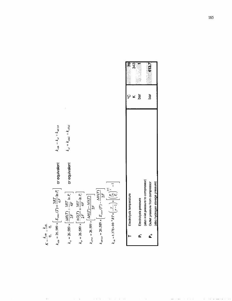
or e
quiv
alen
t
or e
quiv
alen
t
Ele
ctro
lysi
s te
mpe
ratu
re
PI
Ele
ctro
lysi
s pr
essu
re
(als
o in
let p
ress
ure
to c
ompr
esso
r)
Po
Out
let p
ress
ure
from
com
pres
sor
K
bar
bar
I (a
lso
hydr
ogen
sto
rage
pre
ssur
e)
I I
I

Gre
enh
ou
se G
as R
elat
ed R
elat
ive
Co
stIS
avin
g
Var
iabl
e -
CGHG
I
CG
HG
P
CG
HG
~
CG
HG
~
- le
lativ
e an
nual
cos
t/sav
ing
in te
rms
of G
HG
(with
resp
ect t
o ga
solin
e IC
E)
lela
tive
annu
al c
ost/s
avin
g in
term
s of
GH
G
(with
resp
ect t
o g
asol
ine
FCV
with
on-
boar
d pr
oces
sing
)
lela
tive
annu
al c
osth
avin
g in
term
s of
GH
G
(with
resp
ect t
o m
etha
nol F
CV
with
on-
boar
d pr
oces
sing
)
lela
tive
annu
al c
ost/s
avin
g in
term
s of
GH
G
(with
resp
ect t
o hy
drog
en F
CV
from
dec
entr
aliz
ed S
MR
)
lalu
e of
GH
G e
mis
sion
s fro
m a
ltern
ativ
e 1
(Gas
olin
e IC
E)
lalu
e o
f G
HG
em
issi
ons
from
alte
rnat
ive
2
(Gas
olin
e FC
V w
ith o
n-bo
ard
proc
essi
ng)
lalu
e o
f G
HG
em
issi
ons
from
alte
rnat
ive
3
(Met
hano
l FC
V w
ith o
n-bo
ard
proc
essi
ng)
lalu
e o
f GH
G e
mis
sion
s fro
m a
ltern
ativ
e 4
(Hyd
roge
n FC
V fr
om d
ecen
tral
ized
SM
R)
lalu
e o
f GH
G e
mis
sion
s fr
om e
lect
roly
sis
lalu
e o
f G
HG
em
issi
ons
from
ele
ctro
lysi
s pe
r kg
of
H2
Uni
ts
$/yr
$/km
driv
en
$/km
driv
en
$/km
driv
en
$/km
driv
en
$/km
driv
en
$/kg
H2
Val
ue
-883
3
Eco
2 l~
va
lua
tio
n
of C
02
equ
ival
ent e
mis
sion
s I
US
$/to
n C
on
I 20
Loca
tion
For V
anco
uver
, C
anad
a, e
nter
1
For
Los
Ang
eles
,US
A,
ente
r 2
For
Par
is, F
ranc
e, e
nter
3
For a
noth
er lo
catio
n en
ter
4 (O
ther
loca
tion,
spe
cifie
d in
wor
kshe
et "
Site
-Spe
cific
Info
")
Van
couv
er
I 11

To
faci
litat
e th
e un
ders
tand
ing
of t
he v
ario
us v
alue
s di
spla
yed
in th
is m
odel
, a
code
of
colo
rs h
as b
een
used
.
Yel
low
cel
ls id
entif
y in
tera
ctiv
e in
put c
ells
.
Gre
en c
ells
are
non
-inte
ract
ive
cells
that
sim
ply
sum
mar
ize
(in
the
"Inp
ut S
umm
ary"
wor
kshe
et)
the
valu
es e
nter
ed in
all
the
yello
w c
ells
of t
he m
odel
.
Blu
e ce
lls id
entif
y th
e m
ain
outp
ut c
ells
of t
he m
odel
.
Ora
nge
cells
iden
tify
non-
inte
ract
ive
inpu
t cel
ls to
the
mod
el, i
n th
e se
nse
that
thei
r in
form
atio
n co
nten
t can
be
used
as
refe
renc
e fo
r in
tera
ctiv
e in
put,
but t
hey
are
not d
irect
ly li
nked
to a
ny o
ther
cel
ls.

1) N
eed
for
Hyd
rog
en F
uel
2) V
aria
ble
s In
fluen
cin
g C
apita
l + O
&M
Cos
t
Var
iabl
e U
nits
V
alue
Rd
Rat
io o
f pe
ak H
2 pr
oduc
tion
to a
vera
ge d
eman
d
f C
apac
ity fa
ctor
(av
erag
e us
e [h
ours
per
day
] 124
h)
e,
Uni
t cos
t of
elec
troly
zer p
er k
W,
cU
Uni
t cos
t of c
ompr
esso
r per
kW
Out
of H
2 (H
HV
)
D
Equ
ival
ent n
umbe
r of
days
of s
tora
ge
A
Ava
ilabl
e fr
actio
n of
sto
red
hydr
ogen
Su
S
tora
ge c
apita
l cos
t per
kg
of s
tore
d H
2 (H
HV
)
x C
apita
l cos
t of
bala
nce
of p
lant
V
Num
ber o
f veh
icle
s se
wed
by
stat
ion
M
Ave
rage
ann
ual m
ileag
e pe
r veh
icle
fe
Ave
rage
fuel
eco
nom
y
kmly
r km
lkg
H2
Var
iab
les
Invo
lved
in F
inan
cin
g th
e E
lect
roly
sis
Sta
tion
If
trea
ted
as a
hom
e ap
plia
nce,
ent
er 1
100
1920
0 13
5
i, M
ortg
age
inte
rest
rat
e (if
fina
nced
as
an a
pplia
nce)
T,
Per
sona
l tax
rat
e of
hom
e ow
ner
Gen
eral
infla
tion
rate
r A
fter-
tax
real
rate
of
retu
rn o
n in
vest
men
t (in
con
stan
t dol
lars
)
for
hom
e ap
plia
nce
case
for
hom
e ap
plia
nce
case
for
busi
ness
cas
e
for
busi
ness
cas
e
for
busi
ness
cas
e

Gre
enh
ou
se G
as R
elat
ed R
elat
ive
Co
stIS
avin
g
Var
iabl
e -
CGHG
I
CG
HG
P
CG
HG
~
CG
HG
~
- le
lativ
e an
nual
cos
t/sav
ing
in te
rms
of G
HG
(with
resp
ect t
o ga
solin
e IC
E)
lela
tive
annu
al c
ost/s
avin
g in
term
s of
GH
G
(with
resp
ect t
o g
asol
ine
FCV
with
on-
boar
d pr
oces
sing
)
lela
tive
annu
al c
osth
avin
g in
term
s of
GH
G
(with
resp
ect t
o m
etha
nol F
CV
with
on-
boar
d pr
oces
sing
)
lela
tive
annu
al c
ost/s
avin
g in
term
s of
GH
G
(with
resp
ect t
o hy
drog
en F
CV
from
dec
entr
aliz
ed S
MR
)
lalu
e of
GH
G e
mis
sion
s fro
m a
ltern
ativ
e 1
(Gas
olin
e IC
E)
lalu
e o
f G
HG
em
issi
ons
from
alte
rnat
ive
2
(Gas
olin
e FC
V w
ith o
n-bo
ard
proc
essi
ng)
lalu
e o
f G
HG
em
issi
ons
from
alte
rnat
ive
3
(Met
hano
l FC
V w
ith o
n-bo
ard
proc
essi
ng)
lalu
e o
f GH
G e
mis
sion
s fro
m a
ltern
ativ
e 4
(Hyd
roge
n FC
V fr
om d
ecen
tral
ized
SM
R)
lalu
e o
f GH
G e
mis
sion
s fr
om e
lect
roly
sis
lalu
e o
f G
HG
em
issi
ons
from
ele
ctro
lysi
s pe
r kg
of
H2
Uni
ts
$/yr
$/km
driv
en
$/km
driv
en
$/km
driv
en
$/km
driv
en
$/km
driv
en
$/kg
H2
Val
ue
-883
3
Eco
2 l~
va
lua
tio
n
of C
02
equ
ival
ent e
mis
sion
s I
US
$/to
n C
on
I 20
Loca
tion
For V
anco
uver
, C
anad
a, e
nter
1
For
Los
Ang
eles
,US
A,
ente
r 2
For
Par
is, F
ranc
e, e
nter
3
For a
noth
er lo
catio
n en
ter
4 (O
ther
loca
tion,
spe
cifie
d in
wor
kshe
et "
Site
-Spe
cific
Info
")
Van
couv
er
I 11

To
faci
litat
e th
e un
ders
tand
ing
of t
he v
ario
us v
alue
s di
spla
yed
in th
is m
odel
, a
code
of
colo
rs h
as b
een
used
.
Yel
low
cel
ls id
entif
y in
tera
ctiv
e in
put c
ells
.
Gre
en c
ells
are
non
-inte
ract
ive
cells
that
sim
ply
sum
mar
ize
(in
the
"Inp
ut S
umm
ary"
wor
kshe
et)
the
valu
es e
nter
ed in
all
the
yello
w c
ells
of t
he m
odel
.
Blu
e ce
lls id
entif
y th
e m
ain
outp
ut c
ells
of t
he m
odel
.
Ora
nge
cells
iden
tify
non-
inte
ract
ive
inpu
t cel
ls to
the
mod
el, i
n th
e se
nse
that
thei
r in
form
atio
n co
nten
t can
be
used
as
refe
renc
e fo
r in
tera
ctiv
e in
put,
but t
hey
are
not d
irect
ly li
nked
to a
ny o
ther
cel
ls.

1) N
eed
for
Hyd
rog
en F
uel
2) V
aria
ble
s In
fluen
cin
g C
apita
l + O
&M
Cos
t
Var
iabl
e U
nits
V
alue
Rd
Rat
io o
f pe
ak H
2 pr
oduc
tion
to a
vera
ge d
eman
d
f C
apac
ity fa
ctor
(av
erag
e us
e [h
ours
per
day
] 124
h)
e,
Uni
t cos
t of
elec
troly
zer p
er k
W,
cU
Uni
t cos
t of c
ompr
esso
r per
kW
Out
of H
2 (H
HV
)
D
Equ
ival
ent n
umbe
r of
days
of s
tora
ge
A
Ava
ilabl
e fr
actio
n of
sto
red
hydr
ogen
Su
S
tora
ge c
apita
l cos
t per
kg
of s
tore
d H
2 (H
HV
)
x C
apita
l cos
t of
bala
nce
of p
lant
V
Num
ber o
f veh
icle
s se
wed
by
stat
ion
M
Ave
rage
ann
ual m
ileag
e pe
r veh
icle
fe
Ave
rage
fuel
eco
nom
y
kmly
r km
lkg
H2
Var
iab
les
Invo
lved
in F
inan
cin
g th
e E
lect
roly
sis
Sta
tion
If
trea
ted
as a
hom
e ap
plia
nce,
ent
er 1
100
1920
0 13
5
i, M
ortg
age
inte
rest
rat
e (if
fina
nced
as
an a
pplia
nce)
T,
Per
sona
l tax
rat
e of
hom
e ow
ner
Gen
eral
infla
tion
rate
r A
fter-
tax
real
rate
of
retu
rn o
n in
vest
men
t (in
con
stan
t dol
lars
)
for
hom
e ap
plia
nce
case
for
hom
e ap
plia
nce
case
for
busi
ness
cas
e
for
busi
ness
cas
e
for
busi
ness
cas
e

Ixtr
aord
inar
y ex
pen
ses
El
extr
aord
inar
y ex
pens
e 1
n,
year
in w
hich
ext
raor
dina
ry e
xpen
se 1
occ
urs
En
extra
ordi
nary
exp
ense
2
n2
year
in
whi
ch e
xtra
ordi
nary
exp
ense
2 o
ccur
s
EB
extra
ordi
nary
exp
ense
3
n3
year
in
whi
ch e
xtra
ordi
nary
exp
ense
3 o
ccur
s
E4
extr
aord
inar
y ex
pens
e 4
n4
year
in w
hich
ext
raor
dina
ry e
xpen
se 4
occ
urs
E5
extra
ordi
nary
exp
ense
5
n5
year
in w
hich
ext
raor
dina
ry e
xpen
se 5
occ
urs
Ann
ual i
nsur
an
3) V
aria
ble
s In
fluen
cin
g E
nerg
y C
ost
as a
per
cent
age
of t
he to
tal
inst
alle
d ca
pita
l cos
t of t
he
elec
trol
ytic
hyd
roge
n re
fuel
ling
stat
ion
Tl,
Ene
rgy
effic
ienc
y of
ele
ctro
lyze
r
{Ene
rgy
inpu
t e- +
NG
(HH
V)}
q,
Com
pres
sor e
ffici
ency
(with
resp
ect t
o ad
iaba
tic c
ompr
essi
on)
P,-
Ele
ctric
ity p
rice
PNG
N
atur
al g
as p
rice
a
Fra
ctio
n of
ene
rgy
requ
ired
for
elec
trol
ysis
pro
vide
d by
NG
T
Ele
ctro
lysi
s tem
pera
ture
Pi
Ele
ctro
lysi
s pre
ssur
e
(als
o in
let p
ress
ure
to c
ompr
esso
r)
Po
O
utle
t pre
ssur
e fro
m c
ompr
esso
r
(als
o hy
drog
en s
tora
ge p
ress
ure)
Yo
Yo
$/kw
h $/
G J
"C
bar
bar

4) V
aria
ble
s In
fluen
cin
g th
e G
reen
ho
use
Gas
"A
dd
ed C
ost
ISav
ing
" C
om
po
nen
t
Tre
atm
ent
of C
GH
G (add
ed c
ost(
+)
or s
avin
g (-
) du
e to
GH
G e
valu
atio
n)
To e
xclu
de th
e im
pact
of
CG
HG
, on th
e un
it co
st o
f H
2 (U
) T
o in
clud
e C
G~
~
cons
ider
ing
the
alte
rnat
ive
optio
n:
Mo
net
ary
Eva
luat
ion
of
Gre
enh
ou
se G
as E
mis
sio
ns
) E
c02
I~va
lua
tio
n of C
02
equ
ival
ent e
mis
sion
s I U
S$/
ton
C0
21
20
1 0
ente
r 0
Gas
olin
e IC
E,
Gas
olin
e FC
V w
ith o
n-bo
ard
refo
rmin
g,
Met
hano
l FC
V w
ith o
n-bo
ard
refo
rmin
g,
Hyd
roge
n FC
V fr
om d
ecen
tral
ized
SM
R,
ente
r 1
ente
r 2
ente
r 3
ente
r 4
Bas
e C
ase
for
Eac
h O
ther
Fu
el O
ptio
n
Opt
ion
GH
G e
mis
sion
s lit
er o
f ga
solin
e 1
Fu
el E
cono
my
of O
ther
Fu
el O
ptio
ns
Opt
ion
Gas
olin
e IC
E
Gas
olin
e F
CV
on-
boar
d re
form
ing
Met
hano
l FC
V o
n-bo
ard
refo
rmin
g
Hyd
roge
n FC
V fr
om d
ecen
traliz
ed S
MR
liter
of g
asol
ine
equi
v. (
HH
V) p
er 1
00 k
m 4.
19
3.02
Gas
olin
e IC
E
Gas
olin
e FC
V o
n-bo
ard
refo
rmin
g
Met
hano
l FC
V o
n-bo
ard
refo
rmin
g
Hyd
roge
n FC
V fr
om d
ecen
traliz
ed S
MR
g (C
O2 ,,,, )Ik
m d
riven
248
193
162
80
equi
v. (H
HV
) per
100
km
7.30
6.
1 1
4.19
2.
79

Lo
catio
n
I ~a
nc
ou
ve
r I I
For V
anco
uver
, C
anad
a, e
nter
1
Fo
r Lo
s A
ngel
es,U
SA
, ent
er 2
Fo
r P
aris
, Fra
nce,
ent
er 3
Fo
r ano
ther
loca
tion
ente
r 4
5) S
ite-S
pec
ific
Info
rmat
ion
Aff
ectin
g C
om
par
iso
n w
ith O
ther
Fu
ellin
g O
ptio
ns

Aff
ectin
g G
reen
ho
use
Gas
Add
ed C
ost o
r S
avin
g
Ele
ctri
city
Mix
Van
couv
er
L~
ix
I S
ourc
e I
GH
G e
mis
sion
s I
GH
G e
mis
sion
s co
ntrib
utio
n I
%
0
Ele
ctri
city
Mix
Lo
s A
ngel
es
1 5 0
-,
Q1 0 0.
Mix
I
Sou
rce
I G
HG
em
issi
ons
I G
HG
em
issi
ons
cont
ribut
ion
Coa
l
oil
Nat
ural
Gas
Nuc
lear
Hyd
ro
Win
d
Sol
ar
I 85
5 I
0 ~
I~
at
ur
al
Gas
60
5 30
3
(CO
z eq
ulv )/
kwh
del
iver
e
1071
%
(Co
n eq
uw )
/kw
h d
eliv
ere
1071
16 N
ucle
ar
16
I 3
10 H
ydro
4
0 i
g (C
02
,,,,, )/
kwh
del
iver
ed
0 85
5 60
5 16
4 36
1 9
3
g (C
on
equw
)/k
wh
del
iver
ed
118 9
30
0 4 0 0
1.5
Win
d
Q.5
Sol
ar
11 O
ther
36
1 93 0
1 1 0

Ele
ctri
city
Mix
Par
is
l~
ix
I
Sou
rce
I G
HG
em
issi
ons
I G
HG
em
issi
ons
cont
ribut
ion
I Yo
3
Ele
ctri
city
Mix
: (O
ther
loca
tion
)
0 1
1
82
14
3
0
Mix
I
Sou
rce
I G
HG
em
issi
ons
I G
HG
em
issi
ons
cont
ribut
ion
Coa
l
oil
Nat
ural
Gas
Nuc
lear
Hyd
ro
Win
d
Sol
ar
(CO
P eq
ulv )/k
wh
deliv
ere
1071
YO 70
g (C
OP
equl
v )/
kwh
del
iver
ed
32
855
605
16
4 36
193
1 (CO
P ,,,, )
/kw
h de
liver
el
g (
C4
,,,, )
/kw
h d
eliv
ered
Coa
l I
1071
I 750 0 6 13
1 0 0
0 0
10
0
0
20 N
atur
al G
as
605
121
i
855
oil
0
Nuc
lear
Hyd
ro
Win
d
Sol
ar
16
4 36
193
0 0 0 0

To
tal C
ost
of
Ele
ctro
lytic
Hyd
roge
n
Var
iabl
e U
nits
V
alue
U
Uni
t cos
t of
H2
C
Tot
al a
nnua
l cos
t of
H2
Y
Ann
ual H
2 pr
oduc
tion
from
sta
tion
CC
A
nnua
l cap
ital a
nd O
&M
cos
t
Ce
A
nnua
l ene
rgy
cost
CG
HG
A
nnua
l add
ed c
ost(
+) o
r sa
ving
(-)
due
to G
HG
eva
luat
ion
2' C
= c
c + c
e (+C
GH
G)
**
Bec
ause
CG
HG
is a
rel
ativ
e te
rm d
epen
ding
on
the
alte
rnat
ive
optio
n co
nsid
ered
, it
is p
ossi
ble
to in
clud
e or
exc
lude
CG
HG
in th
e to
tal a
nnua
l cos
t of
H2
01
Com
pare
d to
: N
o co
rn p
aris
on
I -.
.-,
. .
I o
incl
ude
CG
HG
cons
ider
ing
the
alte
rnat
ive
optio
n:(
I T
reat
men
t of
CG
HG
I
To e
xclu
de
the
imp
act o
f C
GH
G. on
the
un
it co
st o
f H
2 (U
)
Gas
olin
e IC
E,
Gas
olin
e FC
V w
ith o
n-bo
ard
refo
rmin
g,
Met
han
ol F
CV
with
on
-bo
ard
refo
rmin
g,
Hyd
rog
en F
CV
from
dec
entr
aliz
ed S
MR
,
0 en
ter
0
ente
r 1
ente
r 2
ente
r 3
ente
r 4

4,
If ne
cess
ary,
the
requ
ired
annu
al h
ydro
gen
prod
uctio
n (Y
) cou
ld b
e ca
lcul
ated
usi
ng
the
spec
ific
mile
age
(Mi)
and
fuel
eco
nom
y ((
fJi)
of t
he v
ario
us v
ehic
les
to b
e
serv
ed b
y th
e st
atio
n:
5,
The
fuel
eco
nom
y of
a v
ehic
le (f,
), in
km
driv
en p
er k
g of
H2,
can
be
calc
ulat
ed:
A)
Dire
ctly
from
the
aver
age
ener
gy in
put r
equi
red
(HH
V)
per
km d
riven
fe [k
mlk
g H
2] =
ene
rgy
req
uir
ed (H
HV
) [k
J/km
] / 1
4 1,8
60 [k
J/kg
H2]
B) F
rom
the
equi
vale
nt fu
el e
cono
my
if ga
solin
e (H
HV
) wer
e us
ed,
eith
er in
equ
ival
ent l
iters
of g
asol
ine
per
100
km d
riven
fe [k
mlk
g H
2] =
407
.83
1 Lp
hkm
(u
sing
HH
V v
alue
s fo
r bo
th g
asol
ine
and
H2)
or in
mile
s pe
r U
S g
allo
n of
gas
olin
e eq
uiva
lent
(mpg
ge)
f, [k
mlk
g H
2] =
1.7
339
* m
pg
ge
(u
sing
HH
V v
alue
s fo
r bo
th g
asol
ine
and
H2)
Lphk
m: f
uel e
cono
my
in li
ters
of
gaso
line
equi
vale
nt (H
HV
) per
100
km
m
pgge
: fue
l eco
nom
y in
mile
s pe
r U
S g
allo
n of
gas
olin
e eq
uiva
lent
(HH
V)
For c
onsi
sten
ce in
this
res
earc
h, th
e hi
gher
-hea
ting-
valu
e is
alw
ays
the
one
used
for
gaso
line
met
hano
l and
hyd
roge
n w
hen
usin
g eq
uiva
lent
fuel
eco
nom
y.
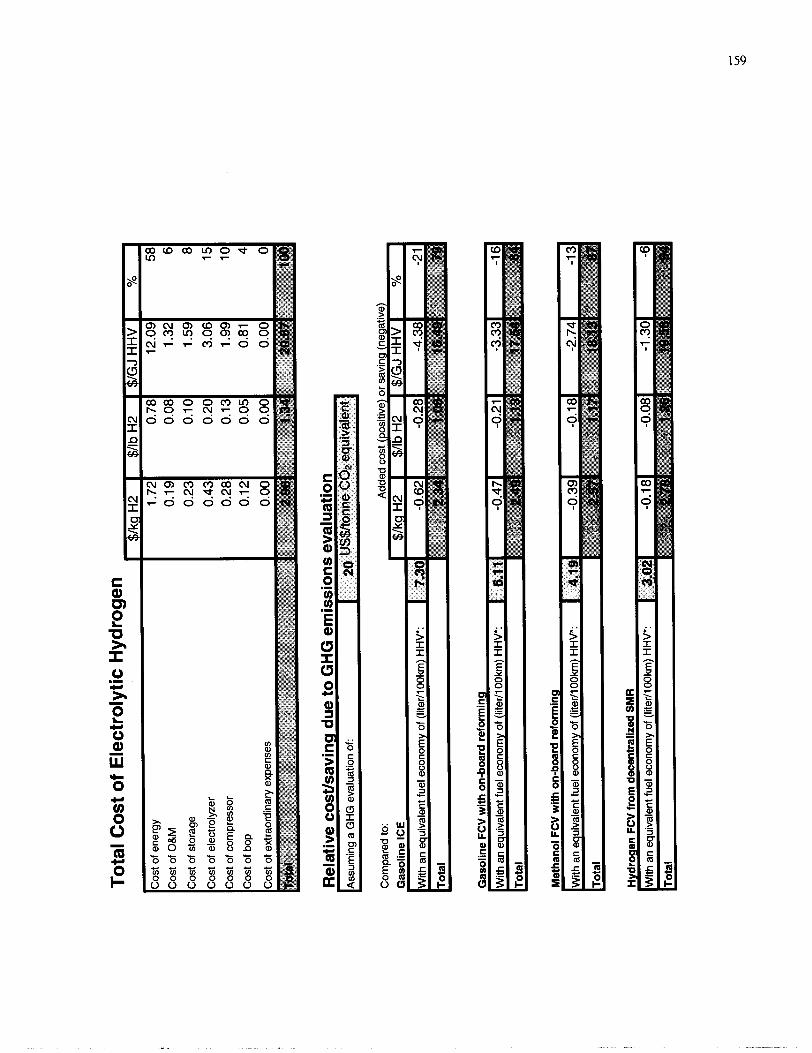
Cos
t of
O&
M
Cos
t of s
tora
ge
Cos
t of
elec
trol
yzer
Cos
t of
com
pres
sor
Cos
t of
bop
To
tal C
ost o
f E
lect
roly
tic H
ydro
gen
Rel
ativ
e co
st/s
avin
g d
ue
to G
HG
em
issi
on
s ev
alu
atio
n
Ass
umin
g a
GH
G e
valu
atio
n of:
I 24)
uS$/
tonn
e C
Q e
quiv
alen
t
Cos
t of e
nerg
y
Com
pare
d to
: A
dded
cos
t (po
sitiv
e) o
r sa
ving
(neg
ativ
e)
Ga
solin
e IC
E
) $/
kg H
2 I
$/lb
H2
I $/
GJ
HH
V I
YO
b m
I
I
I
I
Me
tha
no
l FC
V w
ith
on
-bo
ard
re
form
ing
I
%
58
$/G
JHH
V
12.0
9 $/
kg H
2 1.72
$
/lbH
2
0.78

Co
st C
ompa
riso
n w
ith
Oth
er F
uelli
ng O
ptio
ns
With
an
equi
vale
nt fu
el e
cono
my
of (
liter
1100
km) H
HV
: 7.
30
Ga
solin
e F
CV
with
on-
boar
d re
form
ing
Fue
l cos
t to
cons
umer
Iun
taxe
d G
asol
ine
FCV
with
on
-bo
ard
re
form
ing
I
With
an
equi
vale
nt fu
el e
cono
my
of (
liter
1100
km) H
HV
: 6.
1 1
' Ta
xed
met
hano
l FC
V w
ith o
n-b
oa
rd r
efo
rmin
g
Incl
udin
g ef
fect
of
GH
G e
mis
sion
eva
luat
ion
Add
ed c
ost
I T
otal
l~e
tha
no
l FC
V w
ith o
n-bo
ard
refo
rmin
g
I
Tax
on
fuel
V
anco
uver
With
an
equi
vale
nt fu
el e
cono
my
of (
liter1
1 00k
m)
HH
V:
4.19
' T
axe
d h
ydro
ge
n F
CV
fro
m d
ecen
tral
ized
SM
R
l~
~d
ro
~e
n
FC
V fr
om
dec
entr
aliz
ed S
MR
I
ydro
ge
n F
CV
fro
m d
ecen
tral
ized
ele
ctro
lysi
s
* A
ssum
es m
etha
nol a
nd h
ydro
gen
are
taxe
d at
the
sam
e ra
te p
er u
nit e
nerg
y (H
kU) a
s ga
solin
e

Cap
ital +
O&
M (O
pera
tion
and
Mai
nten
ance
) Cos
t
C,P
e C
S
X
CR
F
CR
F,
Tot
al in
stal
led
capi
tal c
ost o
f H
2 di
spen
sing
sta
tion:
elec
trol
yzer
, com
pres
sor,
H2
stor
age
and
asso
ciat
ed c
ontro
ls
Cap
ital c
ost o
f el
ectro
lyze
r
Cap
ital c
ost o
f com
pres
sor
Cap
ital c
ost o
f sto
rage
Cap
ital c
ost o
f ba
lanc
e of
pla
nt
Cap
ital r
ecov
ery
fact
or
Effe
ctiv
e ca
pita
l rec
over
y fa
ctor
op
A
nnua
l ope
ratin
g an
d m
aint
enan
ce co
sts
ins
Ann
ual i
nsur
ance
t A
nnua
l pro
pert
y ta
xes
% o
f Cca
p
$/yr
%
of C
cap
$/yr
%
of C
,,
Val
ue
1)
Cc=
Cc,
(CR
E+
op
+in
s+t)
+C
R
2)
CC
ap
= (e
+ c +
s + x)
kout
3,
e=
e, *-
'1"
4)
c =
c,
* k,,,
YD
5, s=s *
-*-
" 365
A
6,
CR
F =
d
1 - (1
+ d)
-N
7, C
Rc = C
RF
for
hom
e ap
plia
nce
case
C
RF
, =
1-T,
for
busi
ness
cas
e

" 1
QH
Z~
~X
M
axim
um H
2 flo
w fr
om e
lect
roly
zer
I ~
mj
k I
26.4
93
') 1
kou
t M
axim
um r
ew
ire
d H
2 ~
ow
er o
ut~
ut (H
HW
from
ele
ctro
lvze
r I
kW
I 93.831
Use
ful e
nerg
y ef
ficie
ncy
of e
lect
roly
zer (
excl
udin
g co
mpr
essi
on)
(He
ah
pa
b nf
H7 n
trW
HH
V)
@ 7
5' C)
(Ene
rgy
inpu
t e- +
NG
(HH
V))
Rat
io o
f pea
k H
2 pr
oduc
tion
to a
vera
ge d
eman
d
Cap
acity
fact
or (
aver
age
use
[hou
rs p
er d
ay] 1
24h)
Uni
t cos
t of
elec
troly
zer
per k
W,
Uni
t cos
t of c
ompr
esso
r per
kW
wt o
f H
2 (H
HV
)
Equ
ival
ent n
umbe
r of
days
of s
tora
ge
Ava
ilabl
e fr
actio
n of
sto
red
hydr
ogen
Sto
rage
cap
ital c
ost p
er k
g of
sto
red
H2
(HH
V)
x C
apita
l cos
t of
bala
nce
of p
lant
If tr
eate
d as
a h
ome
appl
ianc
e, e
nter
1
If tr
eate
d as
a b
usin
ess
inve
stm
ent,
ente
r 2
d
Dis
coun
t rat
e
N
Eco
nom
ic re
cove
ry p
erio
d
i, M
ortg
age
inte
rest
rate
(if f
inan
ced
as a
hom
e ap
plia
nce)
Tp
P
erso
nal ta
x ra
te o
f ho
me
owne
r
i G
ener
al in
flatio
n ra
te
r A
fter-
tax
real
rate
of
retu
rn o
n in
vest
men
t (fo
r bu
sine
ss c
ase)
(in c
onst
ant d
olla
rs)
Tb
Bus
ines
s ta
x ra
te
WW
o,
(HH
V)
days
$/kg
H2
%
year
s %
Yo
Yo
Yo
%
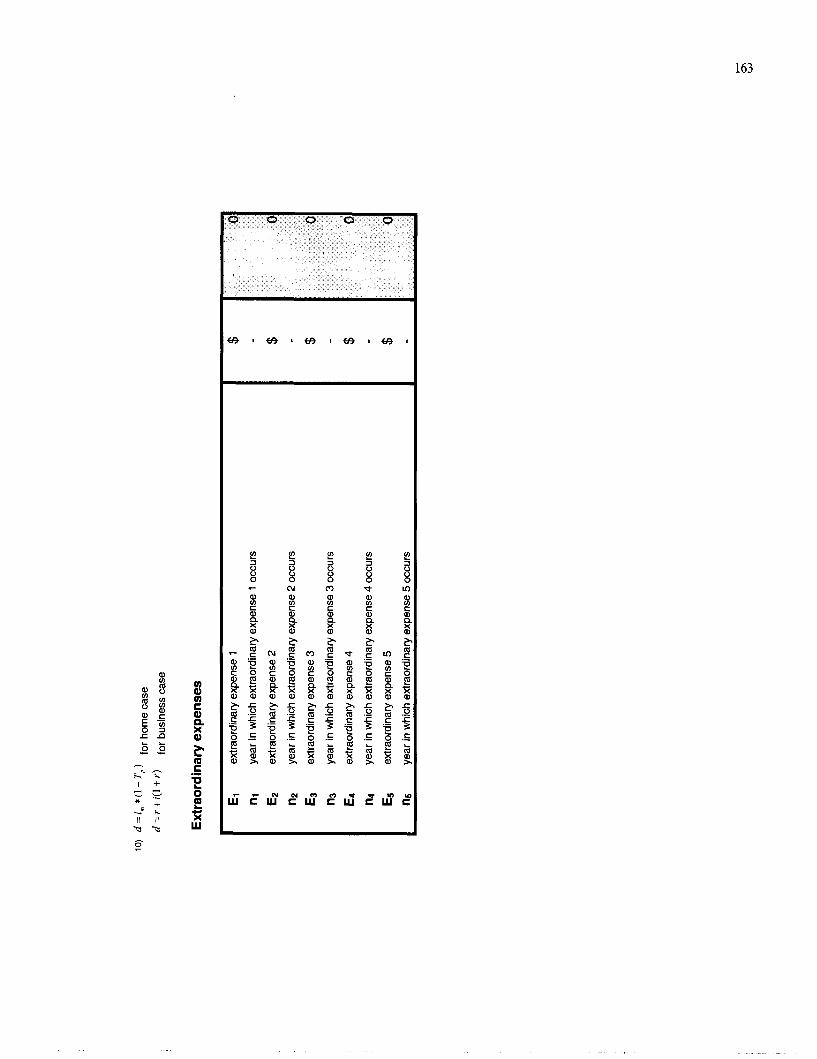
10)
d=
i, *
(l-T
,)
for
hom
e ca
se
=
+ i(
l +
for
busi
ness
cas
e
Ext
rao
rdin
ary
exp
ense
s
El
extr
aord
inar
y ex
pens
e 1
nl
year
in w
hich
ext
raor
dina
ry e
xpen
se 1
occ
urs
E2
extr
aord
inar
y ex
pens
e 2
n2
year
in w
hich
ext
raor
dina
ry e
xpen
se 2
occ
urs
Et
extra
ordi
nary
exp
ense
3
n3
year
in w
hich
ext
raor
dina
ry e
xpen
se 3
occ
urs
E4
extr
aord
inar
y ex
pens
e 4
n4
year
in w
hich
ext
raor
dina
ry e
xpen
se 4
occ
urs
Es
extra
ordi
nary
exp
ense
5
n5
year
in w
hich
ext
raor
dina
ry e
xpen
se 5
occ
urs

Ene
rgy
Cos
t
Var
iabl
e U
nits
V
alue
Ce
Ann
ual e
nerg
y co
st
Ce1
Ann
ual c
ost o
f en
ergy
for
elec
trol
yzer
Ccor
np
Ann
ual c
ost o
f en
ergy
for
com
pres
sor
Spe
cific
ene
rgy
requ
ired
by e
lect
roly
zer a
nd c
ompr
esso
r
Spe
cific
theo
retic
al e
nerg
y re
quire
d by
ele
ctro
lyze
r (e
xclu
ding
com
pres
sor)
(Ass
umin
g no
hea
t rec
over
y fro
m p
rodu
ct g
ases
)
The
oret
ical
ene
rgy
requ
ired
to e
lect
roly
ze w
ater
Req
uire
d ch
ange
in G
ibbs
free
ene
rgy
Req
uire
d he
at fo
r el
ectr
olys
is
The
oret
ical
ene
rgy
requ
ired
to h
eat f
eed-
wat
er to
ele
ctro
lysi
s te
mpe
ratu
re
(Inc
lude
s en
ergy
for
vapo
rizat
ion
at T
empe
ratu
re >
or =
100
C)
Ene
rgy
effic
ienc
y of
ele
ctro
lyze
r
(Spe
cific
ene
rgy
inpu
t (e-
+ N
G (
HH
V))
)
Spe
cific
theo
retic
al e
nerg
y re
quire
d fo
r co
mpr
essi
on
Com
pres
sor e
ffici
ency
(with
resp
ect t
o ad
iaba
tic c
ompr
essi
on)
Ele
ctric
ity p
rice
Nat
ural
gas
pric
e
a
Fra
ctio
n of
ene
rgy
requ
ired
for
elec
trol
ysis
pro
vide
d by
NG
kWh/
kg H
2 kW
h/kg
H2
kWh/
kg H
2 kW
h/kg
H2
kWh/
kg H
2
kWh/
kg H
2
%
kWh/
kg H
2
%
$/k
wh
$/G J
$
/kw
h H
HV

or e
quiv
alen
t
or e
quiv
alen
t
Ele
ctro
lysi
s te
mpe
ratu
re
PI
Ele
ctro
lysi
s pr
essu
re
(als
o in
let p
ress
ure
to c
ompr
esso
r)
Po
Out
let p
ress
ure
from
com
pres
sor
K
bar
bar
I (a
lso
hydr
ogen
sto
rage
pre
ssur
e)
I I
I
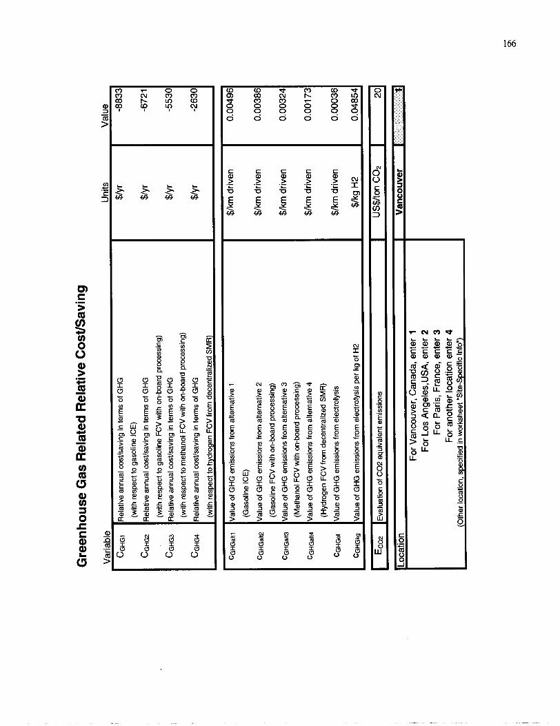
Gre
enh
ou
se G
as R
elat
ed R
elat
ive
Co
stIS
avin
g
Var
iabl
e -
CGHG
I
CG
HG
P
CG
HG
~
CG
HG
~
- le
lativ
e an
nual
cos
t/sav
ing
in te
rms
of G
HG
(with
resp
ect t
o ga
solin
e IC
E)
lela
tive
annu
al c
ost/s
avin
g in
term
s of
GH
G
(with
resp
ect t
o g
asol
ine
FCV
with
on-
boar
d pr
oces
sing
)
lela
tive
annu
al c
osth
avin
g in
term
s of
GH
G
(with
resp
ect t
o m
etha
nol F
CV
with
on-
boar
d pr
oces
sing
)
lela
tive
annu
al c
ost/s
avin
g in
term
s of
GH
G
(with
resp
ect t
o hy
drog
en F
CV
from
dec
entr
aliz
ed S
MR
)
lalu
e of
GH
G e
mis
sion
s fro
m a
ltern
ativ
e 1
(Gas
olin
e IC
E)
lalu
e o
f G
HG
em
issi
ons
from
alte
rnat
ive
2
(Gas
olin
e FC
V w
ith o
n-bo
ard
proc
essi
ng)
lalu
e o
f G
HG
em
issi
ons
from
alte
rnat
ive
3
(Met
hano
l FC
V w
ith o
n-bo
ard
proc
essi
ng)
lalu
e o
f GH
G e
mis
sion
s fro
m a
ltern
ativ
e 4
(Hyd
roge
n FC
V fr
om d
ecen
tral
ized
SM
R)
lalu
e o
f GH
G e
mis
sion
s fr
om e
lect
roly
sis
lalu
e o
f G
HG
em
issi
ons
from
ele
ctro
lysi
s pe
r kg
of
H2
Uni
ts
$/yr
$/km
driv
en
$/km
driv
en
$/km
driv
en
$/km
driv
en
$/km
driv
en
$/kg
H2
Val
ue
-883
3
Eco
2 l~
va
lua
tio
n
of C
02
equ
ival
ent e
mis
sion
s I
US
$/to
n C
on
I 20
Loca
tion
For V
anco
uver
, C
anad
a, e
nter
1
For
Los
Ang
eles
,US
A,
ente
r 2
For
Par
is, F
ranc
e, e
nter
3
For a
noth
er lo
catio
n en
ter
4 (O
ther
loca
tion,
spe
cifie
d in
wor
kshe
et "
Site
-Spe
cific
Info
")
Van
couv
er
I 11

or e
quiv
alen
t
or e
quiv
alen
t
Ele
ctro
lysi
s te
mpe
ratu
re
PI
Ele
ctro
lysi
s pr
essu
re
(als
o in
let p
ress
ure
to c
ompr
esso
r)
Po
Out
let p
ress
ure
from
com
pres
sor
K
bar
bar
I (a
lso
hydr
ogen
sto
rage
pre
ssur
e)
I I
I

Gre
enh
ou
se G
as R
elat
ed R
elat
ive
Co
stIS
avin
g
Var
iabl
e -
CGHG
I
CG
HG
P
CG
HG
~
CG
HG
~
- le
lativ
e an
nual
cos
t/sav
ing
in te
rms
of G
HG
(with
resp
ect t
o ga
solin
e IC
E)
lela
tive
annu
al c
ost/s
avin
g in
term
s of
GH
G
(with
resp
ect t
o g
asol
ine
FCV
with
on-
boar
d pr
oces
sing
)
lela
tive
annu
al c
osth
avin
g in
term
s of
GH
G
(with
resp
ect t
o m
etha
nol F
CV
with
on-
boar
d pr
oces
sing
)
lela
tive
annu
al c
ost/s
avin
g in
term
s of
GH
G
(with
resp
ect t
o hy
drog
en F
CV
from
dec
entr
aliz
ed S
MR
)
lalu
e of
GH
G e
mis
sion
s fro
m a
ltern
ativ
e 1
(Gas
olin
e IC
E)
lalu
e o
f G
HG
em
issi
ons
from
alte
rnat
ive
2
(Gas
olin
e FC
V w
ith o
n-bo
ard
proc
essi
ng)
lalu
e o
f G
HG
em
issi
ons
from
alte
rnat
ive
3
(Met
hano
l FC
V w
ith o
n-bo
ard
proc
essi
ng)
lalu
e o
f GH
G e
mis
sion
s fro
m a
ltern
ativ
e 4
(Hyd
roge
n FC
V fr
om d
ecen
tral
ized
SM
R)
lalu
e o
f GH
G e
mis
sion
s fr
om e
lect
roly
sis
lalu
e o
f G
HG
em
issi
ons
from
ele
ctro
lysi
s pe
r kg
of
H2
Uni
ts
$/yr
$/km
driv
en
$/km
driv
en
$/km
driv
en
$/km
driv
en
$/km
driv
en
$/kg
H2
Val
ue
-883
3
Eco
2 l~
va
lua
tio
n
of C
02
equ
ival
ent e
mis
sion
s I
US
$/to
n C
on
I 20
Loca
tion
For V
anco
uver
, C
anad
a, e
nter
1
For
Los
Ang
eles
,US
A,
ente
r 2
For
Par
is, F
ranc
e, e
nter
3
For a
noth
er lo
catio
n en
ter
4 (O
ther
loca
tion,
spe
cifie
d in
wor
kshe
et "
Site
-Spe
cific
Info
")
Van
couv
er
I 11
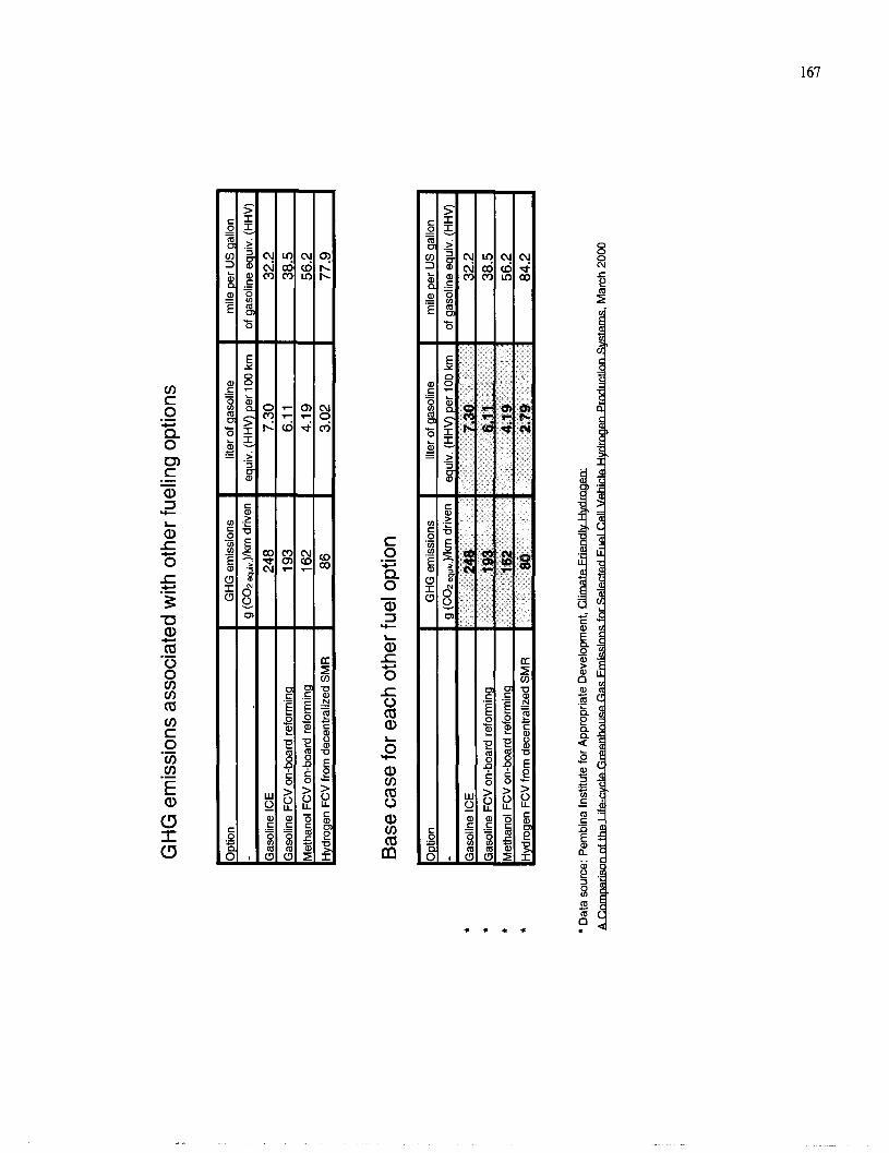
GH
G e
mis
sion
s as
soci
ated
with
oth
er fu
elin
g op
tions
Bas
e ca
se fo
r ea
ch o
ther
fuel
opt
ion
Opt
ion
Gas
olin
e IC
E
Gas
olin
e FC
V o
n-bo
ard
refo
rmin
g
Met
hano
l FC
V o
n-bo
ard
refo
rmin
g
Hyd
roge
n F
CV
from
dec
entr
aliz
ed S
MR
Opt
ion
I G
HG
em
issi
ons
I lit
er o
f ga
solin
e 1
mile
per
US
gal
lon
Dat
a so
urce
: Pem
bina
Inst
itute
for
App
ropr
iate
Dev
elop
men
t, .
. h,
Mar
ch 2
000
GH
G e
mis
sion
s
g (C
op q
uiv
.)lk
t driv
en
248
1 93
1 62
86
liter
of
gaso
line
equi
v. (
HH
V) p
er 1
00 k
m
7.30
6.
1 1
4.19
3.
02
mile
per
US
gal
lon
of g
asol
ine
equi
v. (H
HV
)
32.2
38
.5
56.2
77
.9

GH
G e
mis
sion
s as
soci
ated
with
oth
er fu
elin
g op
tions
Bas
e ca
se fo
r ea
ch o
ther
fuel
opt
ion
Opt
ion
Gas
olin
e IC
E
Gas
olin
e FC
V o
n-bo
ard
refo
rmin
g
Met
hano
l FC
V o
n-bo
ard
refo
rmin
g
Hyd
roge
n F
CV
from
dec
entr
aliz
ed S
MR
Opt
ion
I G
HG
em
issi
ons
I lit
er o
f ga
solin
e 1
mile
per
US
gal
lon
Dat
a so
urce
: Pem
bina
Inst
itute
for
App
ropr
iate
Dev
elop
men
t, .
. h,
Mar
ch 2
000
GH
G e
mis
sion
s
g (C
op q
uiv
.)lk
t driv
en
248
1 93
1 62
86
liter
of
gaso
line
equi
v. (
HH
V) p
er 1
00 k
m
7.30
6.
1 1
4.19
3.
02
mile
per
US
gal
lon
of g
asol
ine
equi
v. (H
HV
)
32.2
38
.5
56.2
77
.9

Site
-Sp
ecifi
c In
form
atio
n
Aff
ectin
g C
om
par
iso
n w
ith O
ther
Fu
ellin
g O
pti
on
s -
Aff
ectin
g C
apit
al C
ost
of
Ele
ctro
lysi
s V
aria
bles
of
the
mod
el a
ffec
ted
Aff
ectin
g E
ner
gy
Co
st o
f E
lect
roly
sis

Aff
ectin
g G
reen
ho
use
Gas
Add
ed C
ost
or
Sav
ing
Tot
al
Ele
ctri
city
Mix
Van
couv
er
Mix
I
Sou
rce
I I
GH
G e
mis
sion
s I G
HG
em
issi
ons
cont
ribut
ion
g (C
OP
equ
l,)/k
Wh
de
liver
ed I
g (C
op eq
ul,
)/kw
h d
eliv
ered
Ele
ctri
city
Mix
Lo
s A
ng
eles
1 S
ourc
e 1
GH
G e
mis
sion
s 1 G
HG
em
issi
ons
cont
ribut
ion
1
Tot
al
%
I t 1
l~o
al
g (C
O;!
equw
)/kw
h d
eliv
ered
1071
g (C
op e,u
l, )/k
Wh
deliv
ered
118
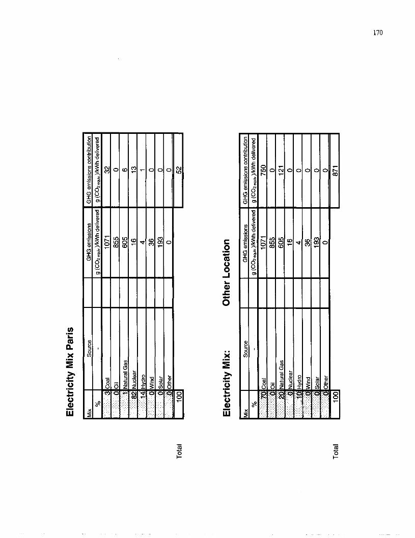
Ele
ctri
city
Mix
Par
is
Tot
al
Tot
al
1 S
ourc
e 1
1 G
HG
em
issi
ons
YO
3
GH
G e
mis
sion
s co
ntrib
utio
n
g (C
op
eq,lv
.)/kW
h de
liver
ed
32
0 0 1
&?
14 0 0
Ele
ctri
city
Mix
: O
ther
Lo
catio
n
Coa
l
I S
ourc
e I
1 G
HG
em
issi
ons
I GH
G e
mis
sion
s co
ntrib
utio
n
g (C
op ,qu
a )/
kwh
del
iver
ed
1071
oil
Nat
ural
Gas
Nuc
lear
Hyd
ro
Win
d
Sol
ar
, Yo
g (C
OP
equn
)/kw
h d
eliv
ered
g
(Con
equl
v )/
kwh
del
iver
ed
7O
i~o
a1
1071
750
855
605
16
4 36
1 93

Appendix D - Base Case Values for
Sensitivity Analysis
Two main sources were used to select base case values for each parameter considered in the
sensitivity analysis. The first one is the 1996 report by the Electrolyser Corporation (now
Stuart Energy Systems) to Ford Motor '. This source offers the advantage of cost projections
from an actual electrolyzer company. The second source is the 1995 report by Directed
Technologies Inc. (DTI) 2. Whenever these two sources are mentioned in the tables below
they are refened to as "Stuart" and "DTI" respectively.
When the base case values are compared to values from "Stuart", they refer to the scenario
that considers a fleet station comprising 10 HVRAs (hydrogen vehicle refbelling appliances),
each designed to serve 4 FCVs, for a total of 40 fleet vehicles supported by the station, for an
annual production of 25,000 HVRAs. Since the mileage of these fleet vehicles is 1.5 times
higher than the one assumed for FCVs in this research, and their fbel economy about 40%
lower, the same station size can be used for the base case of this research, supporting 100
FCVs. Further justification is given in the first table below. When the base case values are
compared to values from "DTI", they refer to the scenario where an electrolytic hydrogen fleet
station is financed by a utility.
The base case and range values for each parameter are presented in four separate tables. The
first one considers the parameters that determine the hydrogen demand for the station. The
other three tables respectively contain the parameters used in the three components of the cost
model: "capital & O&M", "Energy", and "GHG added cost or saving".
Fairlie M. FCV Fuel Suuvlv Infrastructure: The Electrolysis ODtion, Electrolyser, Ltd. Toronto, Canada, December, 1996,105 p.
2 Thomas C.E., Kuhn I.F. Jr. Electrolytic Hvdrogen Production b t t u c t u r e Options and Evaluation. Prepared for the National Renewable Energy Laboratory by Directed Technologies Inc. Report No. NREUTP463-7903, National Renewable Energy Laboratory, Colorado, U.S., 1995,5 1 p.

in the middle of the range considered.
The lower range value V = 2 correspond to a home electrolyzer supporting two FCVs. The upper range value V = 1,000 is of the same order as the average
ce station in the U.S., which serves 165 vehicles per day or about
hydrogen
The base case annual mileage used in this research (19,200 kmlyr) reflects the average annual North American mileage for light-duty vehicles, and is identical to the value used by Stuart and DTI. For fleet vehicles however, Stuart and DTI both use an annual mileage that is 1.5 times higher (28,800 kmlyr).
The base case he1 economy value selected (135 kmikg HZ) is similar to the one provided by Ballard Power Systems for a 5-seater Mercedes A-Class FCV '. The FCVs considered by Stuart had a fuel economy about 40% lower (80 W g ) because they were based on a larger and heavier vehicle.
Table D.l: demand of
Base case values and the fuelling station.
range for parameters used to determine the
' Fairlie M. FCV Fuel Suvvly Infhstructure: The Electrolysis Option, Electrolyser, Ltd. Toronto, Canada, December, 1996,105 p.
Pernbina Institute for Appropriate Development, Climate-Friendlv Hvdrogen Fuel: A Comparison of the Life- cvcle Greenhouse Gas Emissions for Selected Fuel Cell Vehicle Hvdrogen Production Svsterns. Report written with support fiom The David Suzuki Foundation, March 2000,44 p.

DTI suggests designing for two standard deviations fkom the mean as a function of the number of vehicles supported by the station, following a Poisson distribution. DTI applied this rule to a 50-car fleet resulting in Rd = 1.28. The same rule was applied for a 100-car fleet in the base case, giving Rpd = 1.2.
The same rule was also applied to a 1000-car fleet, giving R$ = 1.1 for the lower range value. DTI selected Rpd = 1.5 arbitrarily for a two-car station. This analysis used the same value for the upper range value.
Stuart uses Rpd = 1.6 for fleet terminals up to 100 vehicles, and Q = 2 for a two-car station. However, much more storage capacity was planned by DTI, whch effectively reduces the need for a large surge factor. The base case for this study also assumes high storage capacity
Base case value identical to the one used by DTI in their analysis.
The range corresponds to an operating time of 6 to 24 hours a day
$300/kWout (LHV) at 67.5% efficiency (LHV-basis). It is also coherent with Stuart's estimate of about $ 140/kWe at nominal hydrogen production capacity. This number is based on the combined cost of the electrolyzer and power system, considering the production of 25,000 HVRA units annually.
The lower range value of $100/kW, was estimated simply as half of the base case m t cost.
The upper range value is representative of current estimates for electrolyzer station costs produced in small volumes. Stuart's cost estimate for the first 100 HVRA m t s is in the same range: $700kWe at nominal hydrogen production capacity. Other estimates for NEDO in Japan estimate the total cost of a single fuelling station based on PEM electrolysis at about $1,3001 kW, ', whle Norsk Hydro's estimate for the total cost of a belling station based on AWE is around $800/kW,.~
. . .table continues next page.
1 New Energy and Industrial Technology Development Organization (NEDO). International Clean Energy Network Using Hydrogen Conversion (WE-NET): 1998 Annual Summary Raort on Results. March, 1999. 135 p. Kloed C. "Challenges and Opportunities of Building-Up a Hydrogen Infrastructure". Presented at the Grove Symposium W, London, UK, 9-12 September, 200 1.

the compressor and hydrogen dispenser, considering the production of 25,000 HVRA m t s annually.
Stuart ($357/kg Hz) based on commercially available tanks, considering the production of 25,000 HVRA units annually.
The upper range value is based on various sources in the literature that indicate prices for high-pressure storage tanks, generally in the range of $300-500kg H2, but
can accommodate a one-day shutdown of the stahon.
The upper range value D = 11.4 corresponds to the smallest electrolyzer station
. . .table continues next page.
I Padro C.E.G., Putsche V. S w e y of the Economics of Hydrogen Technologies, MCH Report No. TP-570- 27079, National Renewable Energy Laboratory, Colorado, U.S., 1999,57 p. Ogden J.M. Trospects for Building a Hydrogen Energy Inhstructure". In Annual Review of Enem and the Environment, 1999,24: 227-279.
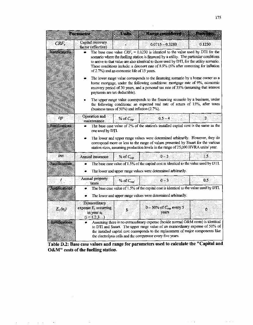
The base case value CRF, = 0.1230 is identical to the value used by DTI for the scenario where the fuelling station is financed by a utility. The particular conditions to arrive to that value are also identical to those used by DTI, for the utility scenario. These condihons include: a discount rate of 8.9% (6% after correcting for inflation of 2.7%) and an economc life of 15 years.
The lower range value corresponds to the financing scenario by a home owner as a home mortgage, under the following conditions: mortgage rate of 9%, economic recovery period of 30 years, and a personal tax rate of 35% (assuming that interest payments are tax deductible).
scenario by a business, under f return of 15%, after taxes
The base case value of 2% of the station's installed capital cost is the same as the one used by DTI.
The lower and upper range values were determined arbitrarily. However, they do correspond more or less to the range of values presented by Stuart for the various station sizes, assuming production levels in the range of 25,000 HVRA Units/ year.
The base case value of 1.5% of the cauital cost is identical to the value used by DTI. (
The lower and upper range values were determined arbitrarily. I
1 The base case value of 1.5% of the capital cost is identical to the value used by DTI.
The lower and utmer range values were determined arbitrarily.
Assurmng there is no extraordmary expense (beside normal O&M costs) is identml to DTI and Stuart. The upper range value of an extraordmary expense of 50% of the installed capltal cost corresponds to the replacement of major components like
O&M" costs of the fuelling station.

. . .table continues next page.
I Thomas C.E., James B.D., Lornax F.D. Jr, Kuhn I.F. Jr. "Fuel Options for the Fuel Cell Vehicle: Hydrogen, Methanol or Gasoline?" International Journal of Hydrogen Energy 25 (2000): 551-567. Ogden J.M. "Developing an Infrastructure for Hydrogen Vehicles: a Southern California Case Study". International Journal of Hydrogen Energy 24 (1999): 709-730.

The base case value of 2 bar is identical to the value used by Stuart. The upper range value of 414 bar corresponds to the maximum storage pressure of 6,000 psi used by both Stuart and DTI. This very high operating pressure could conceivably be achieved, most likely with SPE technology.
The base case value of 414 bar corresponds to the to the maximum storage pressure of 6,000 psi used by both Stuart and DTI. The range of values account for the possibility of storing hydrogen at a lower pressure (e.g. in metal hydrides).
The base case value of $3.00/GJ (HHV) corresponds to approximately $3.30/GJ (LHV), which is somewhere between the price of natural gas for on-site SMR assumed by Thomas et al. ($3.79/GJ (LHV)) and Ogden ($2.80/GJ (LHV)).
The upper range value was determined arbitrarily, to account for possible variations in the market price of the natural gas.
The base case corresponds to the situation where 100% of the energy required by the
\. 4 electrolyzer station comes fiom electricity.
The upper range value corresponds to the case where 100% of the energy required by the electrolyzer station comes fiom natural gas. A new technology like NGASE (natural gas assisted steam electrolysis) would be then necessary to make possible this hypothetical case.
able D.3: Base case values and range for parameters used to calculate the "Energy costs of the fuelling station.
Thomas C.E., James B.D., Lomax F.D. Jr, Kuhn I.F. Jr. "Fuel Options for the Fuel Cell Vehicle: Hydrogen,
2 Methanol or Gasoline?'Intemational Journal ofHydrogen Energy 25 (2000): 551-567. Ogden J.M. 'Developing an Inhstructure for Hydrogen Vehicles: a Southern California Case Study". International Journal of Hydrogen Energy 24 (1999): 709-730.

. . .table continues next page.
1 COze web site: www.co2e.com * Dones R., Gantner U., Hirschberg S. "Greenhouse Gas Total Emissions &om Current and Future Energy and
Heat Supply Systems". In: Proceedings of the 4' International Conference on Greenhouse Gas Control Technologies, Interlaken, Switzerland, 31 Aug.- 2 Sept. 1998, Pergamon, Amsterdam, 1999.891-896.

J
Table D.4: Base case values and range for parameters used to calculate the "GHG Added Cost or Saving" of the fuelling station.
.- -
' Pembina Institute for Appropriate Development, Climate-Friendly Hvdrogen Fuel: A Comarison of the Life- cycle Greenhouse Gas Emissions for Selected Fuel Cell Vehicle Hydrogen Production Svstems. Report written with support •’tom The David Suzuki Foundation, March 2000,44 p.

Appendix E - Site-Specific Information
In Chapter 4, the fbelling cost of using electrolytic hydrogen in a FCV was compared with the
fuelling cost of the equivalent vehicle using gasoline in an ICE, for three different locations:
Vancouver (Canada), Los Angeles (United States), and Paris (France).
The same base case electrolyser station, designed to serve 100 vehicles and assumed to have
the exact same total installed capital cost, was placed in each location. The fbelling cost for
the two fbel options in each city was calculated based on an equivalent driving range for the
hydrogen FCV and gasoline ICE vehicle.
The data used for calculating the fbelling costs of the two options in each city is summarized
in Chapter 4 in a table that is reproduced below. The sources used and calculations performed
to obtain the site-specific information in that table are explained in this appendix.
3.2 12.8 5.9 Electricity mix I Dominated by Dominated by Dominated by
hydroelectric (93%) 1 NG (50%) and coal (1 1%) I nuclear (82%) t Tax on fuel I
* Electricity prices calculated using local tariff schedule for an electrolyzer station supporting 100 hydrogen FCVs,
with a capacity factor of 0.7.
7 Hydrogen taxed at same rate as on gasoline, on an energy content basis (HHV). COP monetary valuation US$20/ton C02-equivalent
Vehicle range 600 kmhll tank on EPA combined driving cycle (Identical for both the gasoline ICE vehicle and the hydrogen FCV)
Fuel economy Gasoline ICE vehicle: 7.30 liter I1 00 km
Hydrogen FCV: 3.02 liter I1 00 km (gasoline equivalent) corresponds to 135 km /kg H2
Table E.l: information compare the price of electrolytic hydrogen gasoline

Electricity Price
The electricity price in US#IkWh was calculated as follows for each of the three locations,
using the same number of daily hours of operation, year-round. The electricity tariffs were
obtained directly fkom the utilities' web sites: respectively BC Hydro in Vancouver ', Southern
California Edison in Los Angeles 2, and ~lectricitk de France in Paris 3.
Amount of hydrogen required in each location: 14,222 kg H2 /year 3 38.9 kg H2 /day
Total energy requirements of station according to base case: 56 kwh k g Hz
Power requirements for the station:
Base case capacity factor f = 0.7 Base case peak-to-average-demand ratio Rpd = 1.2 Average daily hours of operation: 0.7 x 24 hourslday = 16.8 hrslday
Average power requirements: 2,182 kWhlday + 16.8 hrs = 130 kW Maximum powa requirements: 1.2 x 130kW= 156kW
Electricity Price in Vancouver
Electricity Tariff: "Medium Power Schedule 1200", with values fiom 2003
Basic charge: CAN$4.1 5lmonth x 12 = CAN$ 50 /yr
Demand charge: First 35 kW of billing demand per month: Nil
Next 1 15 kW of billing demand per month: $3.32/kW $3.32/kW x 1 1 5kW x 12 months w CAN$ 4,582 /yr
All additional kW of billing demand per month: $6.37/kW
1 BC Hydro web site: www.bchvdro.com Southern California Edison web site: _www.sce.com ~lectricitk de France web site: www.edf.fi

Energy charge: First 14,800 kWh per month @ CAN$O.O649/kWh
All additional kwh per month @ CAN$0.03 12/kWh
[(14,800 x $O.O649/kWh) + (51,570 x $O.O312/kWh)] x 12 mths = CAN$30,834 Iyr
CAN$35,925 Iyr
Total annual electricity requirements of the station: 796,000 kWh
CAN$35,925 /yr 9 796,000 kwh = CAN$O.O451 /kWh
Cmency exchange rate: CAN$ 1 .OO = US$O.7 1
CAN$O.O451 IkWh x 0.71 = US$0.0320 /kWh (excluding all taxes)
Electricity price in Vancouver: 3.2 #/kWh
Electricity Price in Los Angeles
Electricity Tariff "Schedule TOU-GS-2-SOP", with values fiom 2003 (Time-of-use - general service - super off-peak - demand metered )
Customer charge: US$79.25/ month x 12 months = $ 9511yr
Demand charge: Facilities related: P a kW of billing demand p a month: $5.40/kW
$5.40/kWx156kWx12months= $lO,109/yr
Time related: P a kW of billing demand p a month: Summer (3 mth): $1.15/kW; Winter (9 mth): $0.55kW
[($I. 15kW x 3 months) + ($0.55/kW x 9 months)] x 156kW x $ 1,3 10 Iyr $12,370 /yr
Energy charge: Super off-peak: 6 hours a day year-round @ $0.08566 /kWh Mid-peak hours during Summer @ $0.1262 1 /kWh Mid-peak hours during Winter @ $0.12698 /kWh
6 hrslday x 130 kW x $0.08566 /kWh x 365 dayslyr = $24,387 Iyr 10.8 hrslday x 130 kW x $0.12621 /kwh x 91 dayslyr = $16,125 Iyr 10.8 hrslday x 130 kW x $0.12698 /kWh ~ 2 7 4 dayslyr = $48,848 Iyr
$89,360 Iyr
$101,730 /yr

Total annual electricity requirements of the station: 796,000 kWh
$ 101,730 lyr + 796,000 kWh = $0.1278 kwh (excluding all taxes)
Electricity price in Los Angeles: 12.8 PlkWh
Electricity Price in Paris
Electricity Tariff: "Tarif Jaune Base", with values fiom 2003
Demand charge: "Utilisations Longues"
Per kW of billing demand per year: € 47.76kW
€ 47.76kW x 156kW = € 7,450 /yr
Energy charge: Off-peak hours: 8 hours a day year-round Off-peak hours during Winter (5 months) @ € 0.05491 /kwh Off-peak hours during Summer (7 months) @ € 0.02 143 /kWh Other hours during Winter @ € 0.07728 /kWh Other hours during Summa @ € 0.0272 1 /kWh
8hrsldayx 130kW x €0.05491 / kWhx 151 days/yr= € 8 , 6 2 3 1 ~ 8 hrslday x 130 kW x € 0.02 143 /kWh x 21 4 dayslyr = € 4,769 /yr 8.8 hrslday x 130 kW x € 0.07728 /kWh x 151 dayslyr = € 13,350 /yr 8.8 hrdday x 130 kW x € 0.02721 /kwh x 214 dayslyr = € 6,661 /yr
€ 33,403 /yr
€ 40,853 /yr
Total annual electricity requirements of the station: 796,000 kwh
Currency exchange rate: € 1 .OO = US$ 1 .15
€ 0.05 13 /kWh x 1.15 = US$0.0590 /kwh (excluding all taxes)
Electricity price in Paris: 5.9 #/kwh

Electricity Mix
The electricity mix for Vancouver and Paris were obtained from the web site of their
respective power utility: BC Hydro and ~lectricitt de France. For Los Angeles, the electricity
mix was obtained fiom a report of the California Energy Commission, 1
Gasoline Price and Taxes
The gasoline price and taxes for each location were estimated based on data from a report of
the International Energy Agency.
' Wetherall R. "2001 Net System Power Calculation (2001 California Power Mix)", California Energy Commission, April, 2002.
2 International Energy Agency (IEA), World Enerm Outlook 1998 Edition, IEAIOECD, Paris, France, 1999.