a systematic approach to design high-performance feed drive systems

A systematic approach to design high-performance feed drive systems

Min-Seok Kima, Sung-Chong Chungb,*

aDepartment of Mechanical Design and Production Engineering, Hanyang University, 17 HaengdangDong, SungdongGu, Seoul 133-791, South KoreabSchool of Mechanical Engineering, Hanyang University, 17 HaengdangDong, SungdongGu, Seoul 133-791, South Korea

Received 20 October 2004; accepted 28 January 2005

Available online 14 March 2005

Abstract

A systematic design methodology for the mechatronic system composed of mechanical and control subsystems is proposed to design high-

speed and high-precision feed drive systems. Strict mathematical modeling and identification processes of the subsystems are performed in

this paper. Parametric studies and circular motion experiments in the x–y table are conducted to investigate the influence of interactions on

the performance of feed drive systems. Based on analyses of the system performance according to design and operating parameters, a

nonlinear constrained optimization problem including the relevant subsystem parameters of the feed drive system is formulated. The multi-

objective optimization procedure and normalization technique are introduced in the design process. A Pareto optimum solution set is applied

to investigate the relationships between objective functions. The effectiveness of the proposed design methodology is verified through

numerical case studies.

q 2005 Elsevier Ltd. All rights reserved.

Keywords: Abbe offset; Contour error; Digital control; Feed drive system; Integrated design; Mechatronic system; Multi-objective optimization; Pareto

optimum; Stability; x–y table; z transform

1. Introduction

High-speed/precision feed drive systems have been rapidly

adopted in aerospace, semiconductor, die and mold manu-

facturing industries. The need for the high performance feed

drive systems in manufacturing industries comes from the

demand for higher productivity and benefits in machining

processes such as good surface finish, improved chatter

stability and tool life. Feed drive systems in the semiconductor

industry require high-speed motion of 120 m/min peak speed

and 30 m/s2 rated acceleration. High-speed machine tools

require the feed drive systems providing more than 40 m/min

speed and 20 m/s2 peak accelerations [1,2]. However, these

specifications exceed the axis motion capabilities of conven-

tional feed drive systems. It is indispensable to devise an

advanced design methodology to fabricate high-precision/

speed feed drive systems.

Feed drive systems consist of several subsystems such as

force transmission mechanisms, actuators, sensors,

0890-6955/$ - see front matter q 2005 Elsevier Ltd. All rights reserved.

doi:10.1016/j.ijmachtools.2005.01.032

* Corresponding author. Tel.: C82 2 2290 0444; fax: C82 2 2298 4634.

E-mail address: [email protected] (S.-C. Chung).

controllers and amplifiers. Many studies concerning the

design and performance improvement of feed drive systems

have been reported so far [3,4]. Most of the studies are

performed based on the component design methodology,

which focus solely on the design or optimization of each

subsystem as shown in Fig. 1(a). However, performance of

feed drive systems depends upon not only the characteristics

of each subsystem but also the interaction among the

subsystems. This leads to the conclusion that it is impossible

to achieve maximum performance of the feed drive systems

through the component design methodology. Therefore, in

order to design high-performance feed drive systems, a

systematic design approach as shown in Fig. 1(b) is required

in which both mechanical and control subsystems are

simultaneously considered in the design process.

Some systematic design approaches have been reported

[5,6]. The integrated mechanism/control design method-

ology, which focuses on the pre-design of feed drive systems

related to motion systems, has been proposed [5]. However,

information about controller modification and dimensional

data for the mechanical subsystems, such as ballscrew

diameter and lead, were not included explicitly in the

research. The total tuning method for NC feed drive systems

has been proposed to reduce contouring errors of CNC

International Journal of Machine Tools & Manufacture 45 (2005) 1421–1435

www.elsevier.com/locate/ijmactool

http://www.elsevier.com/locate/ijmactool

Notation

Am gain margin of a feed drive system (dB)

A�m allowable gain margin (dB)

amax maximum acceleration of a table (m/s2)

Bm viscous damping coefficient of a motor shaft

(N m s/rad)

Btb width of a table (m)

Bt viscous damping coefficient of a table (N s/m)

C1(z) discrete transfer function of a position controller

C2(z) discrete transfer function of a velocity controller

c1–4 weighting factors of a multi-objective function

Da Abbe offset (m)

Daa double the Abbe offset (m)

Daa0 initial value of the Abbe offset (m)

D�aa Daa/Daa0

Dbs ballscrew diameter (m)

Dcp coupling diameter (m)

Dc(z) characteristic polynomial of a feed drive system

Ebs elastic modulus of a ballscrew (Pa)

Elg elastic modulus of a linear guide (Pa)

Er contour error ratio

Er0 initial value of the contour error ratio

E�r (Er/Er0)2

Etb elastic modulus of a table (Pa)

e feedback error of a feed drive system (m)

Fx;y;zc external force vector (N)

Fd driving force (N)

Fw load due to table and workpiece weight (N)

F(z) discrete transfer function of a feedforward

controller

Gbs shear modulus of a ballscrew (Pa)

Gcp shear modulus of a coupling (Pa)

Gc(z) closed-loop discrete transfer function of a feed

drive system

Gm(s) transfer function of a mechanical subsystem in

continuous domain

Gm(z) Gm(s)/s in discrete domain

GmðzÞ input transfer function of the ARMAX model

Go(z) open-loop discrete transfer function of a feed

drive system

Gsat(z) discrete saturation transfer function of a feed

drive system

g1–8 vector of inequality constraints

HmðzÞ noise transfer function of the ARMAX model

Ibs moment of inertia of a ballscrew (m4)

Ilg moment of inertia of linear guides (m4)

Itb moment of inertia of a table (m4)

J cost function in the identification process

Jeq equivalent inertia of a feed drive system (kg m2)

Jeq0 initial value of the equivalent inertia (kg m2)

J�eq Jeq/Jeq0

Jm inertia of rotating elements (kg m2)

Jrt rotor inertia of a motor (kg m2)

Kemf back-e.m.f. constant of a motor (Vrpm/rpm)

Keq equivalent stiffness of a feed drive system (N/m)

Kff velocity feedforward controller gain (V/V)

Kl equivalent stiffness in the axial direction (N/m)

Knt nut stiffness (N/m)

Kpp proportional gain of a position controller (V/V)

Ksb stiffness of a support bearing (N/m)

Kt torque constant of a motor (N m/Arms)

Kvp proportional gain of a velocity controller (V/V)

Kvi integral gain of a position controller (V/V)

Kq equivalent stiffness in the radial direction

(N m/rad)

ke spring constant of an elastic foundation beam

Lbs ballscrew length (m)

Lcp coupling length (m)

Llg length of a linear guide (m)

Lm inductance of a motor amplifier (H)

Lsp distance between linear guides (m)

Lstr stroke of a feed drive system (m)

Ltb table length (m)

l ballscrew lead (m)

Mt table mass (kg)

n order of a closed-loop system

OP normalized multi-objective function for the

Pareto optimum method

OM multi-objective function

OMN normalized multi-objective function

Pb axial buckling load of a ballscrew (N)

R conversion ratio of linear-to-rotational motion

Ri radius of a circular motion command (m)

Rm resistance of a motor amplifier (U)

Ro radius of a circular motion output (m)

Ti sampling period of a reference input (s)

Tmax maximum torque of a motor (N m)

Ts sampling period (s)

Vc critical velocity of a ballscrew (m/s)

Vmax maximum velocity of a feed drive system (m/s)

Vt reference voltage referring to torque reference t

(V)

vt table velocity (m/s)

vt estimated velocity of a table (m/s)

W1,2 weighting factors of a multi-objective function

for the Pareto optimum method

xc position command (m)

xs transverse distance of a nut (m)

xss steady-state output of a feed drive system (m)

xt transverse distance of a table (m)

x1–7 vector of design variables

xL1–7 lower limit of design variables

xU1–7 upper limit of design variables

aa angular error (rad)

3 Abbe error (m)

M.-S. Kim, S.-C. Chung / International Journal of Machine Tools & Manufacture 45 (2005) 1421–14351422

fm phase margin of a feed drive system (dB)

f�m allowable phase margin (degree)

da allowable structural deformation error (m)

dc structural deformation error (m)

h efficiency of a driving mechanism

4 vector of a regressor

qm rotational angle of a motor shaft (rad)

qs rotational angle of a ballscrew (rad)

rbs ballscrew density (kg/m2)

rtb table density (kg/m2)

t torque reference (N m)

tm driving torque of a motor (N m)

ti time constant of an integral controller (s)

tmaxm maximum torque applied to the motor (N m)

tmaxc maximum magnitude of a control input (N m)

x white noise

uB bandwidth of a feed drive system (rad/s)

uB0 initial value of the bandwidth (rad/s)

u�B uB0/uB

ub natural frequency of a ballscrew shaft (rad/s)

ug gain crossover frequency (rad/s)

ui rotational speed of reference input (rad/s)

up phase crossover frequency (rad/s)

us sampling frequency (rad/s)

uwB bandwidth of a feed drive system in w-domain

(rad/s)

umaxm maximum velocity of a motor (rpm)

Fig. 1. Component design vs. systematic design approaches.

M.-S. Kim, S.-C. Chung / International Journal of Machine Tools & Manufacture 45 (2005) 1421–1435 1423

machine tools [6]. However, the proposed tuning process was

not an automatic design process but a conventional graphic-

interface process using the JK-map, which supports

designers to know the current states of servo performance

and the way to satisfy the desired performance.

In this paper, an integrated design methodology as a

systematic design concept is proposed to design high-

performance feed drive systems. Strict mathematical model-

ing of subsystems of an x–y table is performed first. An

accurate identification process is conducted to verify the

obtained dynamics of the x–y table. Integration of the

subsystems is performed to formulate evaluative factors of

the feed drive system in terms of geometric errors, contour

error, relative stability conditions and so on. Parametric

studies and circular motion experiments on the x–y table are

conducted for better understanding of the influence of

interaction among subsystems on the system performance.

A nonlinear constrained optimization problem including

relevant subsystem parameters and the evaluative factors of

the feed drive system is formulated. A multi-objective

optimization method with non-dimensional variables is

applied to the optimization process. Finally, integrated

design procedures according to various design consider-

ations are conducted. In addition, a Pareto optimum solution

set [7,8] is presented in order to investigate relationships

between objective functions. The integrated design method-

ology provides not only useful knowledge of system

behavior according to subsystem characteristics but also

practical design results such as values of controller gains and

structural dimensions.

This paper presents the modeling and identification

procedures of subsystems in Sections 2 and 3, respect-

ively. In Section 4, evaluative factors of the feed drive

system are derived. Parametric studies and circular motion

experiments are provided in Section 5. Formulation of the

integrated design problems is described in Section 6.

Section 7 describes results of the integrated design and a

Pareto optimum solution set. Conclusions are described in

Section 8.

2. Modeling of feed drive systems

Accurate models of the mechanical and control sub-

systems are indispensable to perform the systematic design

satisfactorily. Mechanical characteristics of a feed drive

system such as overall flexibility, stiffness, natural

frequency and inertia affect significant effects to the design

Fig. 3. Stiffness of the support bearing according to ballscrew diameters.

Fig. 2. Freebody diagram of a feed drive system.


optimization. Mathematical models of the mechanical

subsystem are generally constructed by developing

equations of motion between the motor and components

of the feed drive system. Fig. 2 shows a freebody diagram of

the mechanical subsystem.

In Fig. 2, Jm is the inertia of rotating elements composed

of the motor rotor, coupling and ballscrew inertias. qm and qs

are rotational angles of the motor shaft and the ballscrew,

respectively. tm is the driving torque of the motor. xs and xt

are transverse distances of the nut and the table, respect-

ively. And Mt is the table mass, Fd is the driving force acting

on the mechanical component. R is a conversion ratio of

linear-to-rotational motion. Kl is the equivalent axial

stiffness composed of the ballscrew, nut and support bearing

stiffnesses. Kq is the equivalent torsional stiffness composed

of the ballscrew and the coupling.

Kl Z4Lbs

pEbsD2bs

C1

Knt

C1

2Ksb

� �K1

(1)

Kq Z32Lbs

pGbsD4bs

C32Lcp

pGcpD4cp

!K1

(2)

where Lbs and Dbs are length and diameter of a ballscrew,

respectively. Lcp and Dcp are length and diameter of a

coupling, respectively. And Ebs and Gbs are elastic and shear

moduli of a ballscrew, respectively. Gcp is shear modulus of

a coupling. Knt and Ksb are stiffnesses of the nut and the

support bearings, respectively (refer to Appendix A). The

equivalent inertia Jeq and stiffness Keq of the feed drive

system are described as Eqs. (3) and (4), respectively

Jeq Z R2Mt CJm (3)

Keq ZR2

h

1

Kq

C1

Kl

� �K1

(4)

where h is efficiency of the driving mechanism. It is

assumed that the stiffnesses of the support bearings and the

nut are proportional to the ballscrew diameter. Fig. 3 shows

the relationship between ballscrew diameters and stiffnesses

of the support bearings obtained from technical data [9].

From the above equations and Fig. 2, the mechanical

subsystem model of a feed drive system between the

reference voltage Vt related to torque reference t and table

velocity vt is derived as Fig. 4.

In Fig. 4, (LmsCRm)K1 represents dynamics of a motor

amplifier. Lm and Rm are inductance and resistance of the

amplifier, respectively. Kt and Kemf are the torque and back-

e.m.f. constants, respectively. Bm and Bt are the viscous

damping coefficients of a motor and a table, respectively.

Because Rm/Lm is much smaller than Bm/Jm, it is reasonable

to neglect the amplifier dynamics in the mechanical

subsystem model. Transfer function of the mechanical

subsystem Gm(s) between torque command and the table

velocity is given by

GmðsÞ ZRKtKeqh

s3 Cp1s2 Cp2s Cp3

p1 ZJmBt C ðKtKemf CBmÞMt

JmMt

;

p2 ZðKtKemf CBmÞBt

JmMt

CðJmh CR2MtÞKeq

JmMth

p3 ZðKtKemf CBmÞKeq

JmMt

CR2BtKeq

JmMth; R Z

l

2p

(5)

where l is the ballscrew lead.

PID feedback controllers are generally used to compen-

sate for steady-state error and disturbances such as external

loads and friction forces. However, the PID controllers have

several drawbacks such as poor tracking performance and

severe overshoot. A direct velocity feedforward controller

adding a velocity command to the velocity feedback loop

improves tracking performance and reduces overshoot.

Therefore, a two-degree-of-freedom (2-DOF) controller

composed of a PID feedback controller and a simple direct

feedforward controller is adopted in this paper.

In general, a controller is designed in the continuous-time

domain, s-domain, and implemented in the discrete-time

domain, z-domain, through various transformation

methods. However, discrepancies between the two control-

lers exist whatever transformation methods are used.

Fig. 4. Mechanical subsystem model including amplifier dynamics.

Fig. 5. Block diagram of the position control loop.


Therefore, although performance of a controller designed in

the continuous time domain is proper, there is a practical

limitation to implement to the digital controller. In this paper,

a 2-DOF controller is designed and implemented in the

discrete time domain. When the controller is designed

directly in z-domain, quantization errors of controller gains

are able to be reduced because the controller to be

implemented has poles and zeros that are no longer crowded

near the zZ1. Fig. 5 shows the block diagram of the control

subsystem.

In Fig. 5, xc is a position command and e is a feedback

error. Transfer functions consist of the control subsystem

are given by

C1ðzÞ Z Kpp; C2ðzÞ Z Kvp 1 CKviz

z Kti

� �;

FðzÞ Z Kff

z K1

Tsz

� � (6)

where C1(z) is the position controller, C2(z) is the velocity

controller, and F(z) is the feedforward controller. Kff is the

velocity feedforward controller gain, Kpp is the position

controller gain, Kvp and Kvi are the proportional and integral

gains of the velocity controller, respectively. Ts is the sampling

period and ti is the time constant of the integral controller.

The discrete transfer function Gm(z) is obtained by

applying a zero-order hold equivalent method to the

mechanical subsystem model Gm(s)/s as

GmðzÞ Z ð1 KzK1ÞZGmðsÞ

s2

� �(7)

From Eqs. (1)–(7) and Fig. 5, the open-loop transfer

function Go(z) and the closed-loop transfer function Gc(z) of

the feed drive system are given by Eqs. (8) and (9),

respectively.

GoðzÞ ZeðzÞ

xcðzÞ

ZC2ðzÞGmðzÞ½C1ðzÞCFðzÞ�Tsz

ð1 KFðzÞC2ðzÞGmðzÞÞTsz CC2ðzÞGmðzÞðz K1Þ

(8)

GcðzÞ ZxtðzÞ

xcðzÞ

ZC2ðzÞGmðzÞ½C1ðzÞCFðzÞ�Tsz

ð1 CC1ðzÞC2ðzÞGmðzÞÞTsz CC2ðzÞGmðzÞðz K1Þ

(9)

An interpolator in which reference trajectories are

generated plays an important role to the performance of

feed drive systems [10]. For simplicity, a trapezoidal

velocity profile for acceleration and deceleration is

considered in this paper. Since maximum acceleration

is specified as a design parameter described in Section 6,

parameters of the trapezoidal velocity profile are easily

determined by simple equations. In addition, an interp-

olator design procedure is separated from the design

procedure in a viewpoint of the integrated design

concept, because it is not required to consider design

information of the feed drive system during the

interpolator design. In this paper, therefore, it is assumed

that an interpolator has already been designed so that

generated trajectories have smooth profiles to avoid

excitation of the natural modes in the mechanical

subsystems.

3. Identification of the feed drive system

In order to verify the obtained mathematical model, an

accurate identification process of the mechanical subsystem

is conducted Auto Regressive Moving Average with

eXogenous (ARMAX) model [11] is used for the identifi-

cation. Parameters of the ARMAX model given by Eq. (10)

are estimated by using a weighted least squares penalty

function method in the frequency domain as described in

Eq. (11).

vtðkÞ Z GmðzÞtðkÞC HmðzÞxðkÞ (10)

Jð4Þ Z1

N

XN

kZ1

fvtðkÞK vtðk;4Þg2 (11)

where GmðzÞ is input transfer function, HmðzÞ is the noise

transfer function, x(k) is a white noise entering the system, J

is a cost function, vt is the estimated velocity of a table.

Table 1

Specifications of the x–y table

Specifications Unit Value

Rated power of motor W 400

Maximum torque of motor N m 3.82

Maximum speed of motor rpm 5000

Table size m 0.3!0.3

Stroke (X!Y) m 0.3!0.3

Guide type – Rolling guide

Ballscrew diameter m 0.016

Ballscrew lead m 0.005

Fig. 7. Frequency response plots of the mechanical subsystems.


A vector of the regressor 4 is given by

GmðzÞ Zb1z Cb2z2 C/Cbnb

znb

1 Ca1z C/Canazna

4 Z ½ b1 b2 / bnba1 a2 / ana

�T ð12Þ

Since feed drive systems have nonlinear effects such as

inherent frictions and backlash, it is difficult to identify an

accurate mechanical subsystem model of the feed drive

system. To minimize these effects, a biased-square input

signal is used for the excitation [12]. An input signal

composed of a Gaussian pseudo-random binary sequence is

used as the torque command while the rotational motor

velocity is synchronously collected as an output signal.

The identification process is applied to the x–y

table equipped with a ballscrew driven mechanism using

AC-servo motors and amplifiers, encoders, digital I/O

interfaces, and a PC-based controller. Specifications and

configuration of the x–y table are shown in Table 1 and

Fig. 6, respectively.

A transfer function model GmðzÞ is obtained by using

MATLAB System Identification Toolbox [13]. Fig. 7 shows

frequency response functions of the mechanical subsystems

described in Eqs. (5) and (12). In Fig. 7, it is assumed that

Bm and Bt of the mechanical model given by Eq. (5) are

0.00001 and 0.0001, respectively. From the identification

results, it is confirmed that the mechanical subsystem model

for the systematic design process has been reliably derived.

Fig. 6. Configuration of the x–y table.

4. Evaluative factors of feed drive systems

4.1. Geometric errors

Feed drive systems generally have moving pairs that

move relative to each other. There is an angular error aa if

there is clearance between the ballscrew and nut of a feed

drive system as shown in Fig. 8. The angular error, which is

the worst type of the geometric error in the feed drive

system, is proportionally amplified by the distance Da, Abbe

offset, between the central axis of the ballscrew and the

upper surface of a table. Based on the configuration of the

feed drive system shown in Fig. 8, the Abbe offset is

represented as

Da Z Htb CDbs

2(13)

where Htb is the height of the table. This results in an axial

positioning error called Abbe error 3 as shown in Fig. 8. In

order to design high-precision feed drive systems, the Abbe

error should be considered in the design process [14]. Based

on the configuration of the x–y table shown in Fig. 6, the

actual Abbe offset Daa that will be used in the design process

is double the length of Da.

Fig. 8. Abbe offset and Abbe error in a feed drive system.


4.2. Contour error ratio

In a circular motion of a feed drive system, a motion

command for each axis is given as a sinusoidal signal of

which z-transformation is given by

xcðzÞ Z ZfRi sinðuikTiÞg ZRi sinðuiTiÞ

z2 K2 cosðuiTiÞz C1(14)

where Ti is the sampling period of the reference input, Ri and

ui are radius and rotational speed of the circular motion

command, respectively. Amplitude of the system output at

the steady-state xss becomes the radius of an actual circular

motion Ro as

xss Z Ro Z limz/1

fð1 KzK1ÞGcðzÞxcðzÞg (15)

Therefore, a contour error ratio Er of the feed drive

system related to the circular motion is defined by

Er ZRi KRo

Ri

Z 1 KRo

Ri

Z 1 K

ffiffiffiffiffiffiffiffiffiffiffiffiffiffiffiffiffiffiffiffiffiffiffiffiffiffiffiffiffiffiffiffiffiffiffiffiffiffiffiffiffiffiffiffiffiffiffiffiffiffiffiffiffiffiffiffiffiffiffiffiffiffiffiRefGcðe

juiTiÞg2 C ImfGcðejuiTiÞg2

q(16)

In Eq. (16), Er!0 means that the radius of an actual

circular motion is larger than the command radius, which is

referred to the radius increase error. On the other hand, ErO0

means that the radius of an actual circular motion is smaller

than the command radius, which is referred to the radius

decrease error.

4.3. Stability and response

In order to guarantee the stability of the designed feed

drive systems when there are uncertainties in the modeling

process, nominal and relative stability criteria represented

as gain margin Am and phase margin fm must be considered

as shown in Eqs. (17) and (18), respectively.

jzij!1; zi Z fz : DcðzÞ Z 0g for i Z 1–n (17)

Am Z20log10

1

jGoðejupTsÞj

; up Zminfu ::GoðejuTsÞZKpg

fm Z:fGoðejugTsÞgCp; ug Zminfu : jGoejuTs jZ1g

(18)

where ug is a gain crossover frequency, up is a phase

crossover frequency, Dc(z) and n are the characteristic

polynomial and the order of the closed-loop transfer

function Gc(z), respectively.

Speed of response of the designed feed drive system

is verified from the system bandwidth. However, it is

difficult to obtain an analytical expression of bandwidth

in z-domain, because z is related to ju through ejuTs . In

order to derive the explicit expression of the system

bandwidth in z-domain, a bilinear transformation in

w-plane is required [15]. The w-transformation transforms

the unit circle back to the left-hand side of the complex

plane. If the w-transformation is used, the bandwidth

obtained in terms of Gc(w) is described as uwB. The

bandwidth uB of the feed drive system in the z-domain is

given by

uwB Z uw : j½GcðwÞ�wZjuwj Z

1ffiffiffi2

p

�

uB Zus

ptanK1 puwB

us

(19)

where us is a sampling frequency.

4.4. Actuator and controller saturation

In general, it is known that the best tracking and

disturbance rejection performances of the feed drive

system are achieved by the selection of allowable

maximum controller gains. However, actuators should

fall into saturation when the maximum gain is used,

which renders the system nonlinear and the linear

analysis invalid. Therefore, saturated conditions of the

control subsystem and the maximum allowable torque

applied to the actuator must be included in the design

process. The maximum torque applied to the motor tmaxm

and the maximum magnitude of a control input tmaxc are

given by

tmaxm Z max Jeq

d2

dt2q Z

Jeq

R

d2

dt2xc

�

Z1

2R½2Jm CrtbBtbLtbðDaa KDbsÞR

2�amax (20)

tmaxc Z maxfjtðzÞjzZejuTs g Z maxfnjGsatðe

juTsÞxcðejuTsÞjg

(21)

where amax is the maximum acceleration of the table, rtb,

Ltb and Btb are density, length and width of the table,

respectively. The saturation transfer function Gsat(z) can

be calculated from Fig. 5 as follows:

GsatðzÞ ZtðzÞ

xcðzÞ

ZC2ðzÞ½C1ðzÞCFðzÞ�Tsz

ð1 CC1ðzÞC2ðzÞGmðzÞÞTsz CC2ðzÞGmðzÞðz K1Þ

(22)

4.5. Resonance frequency and structural deformation error

Since the critical speed of a feed drive system leads to

resonance, the critical speed of a ballscrew shaft estimated

from the natural frequency of a bar element, where the

fixed-ends boundary condition is applied, must be included

in the integrated design procedure. The critical speed Vc is

Fig. 9. Effects of mechanical-control interaction to contour error ratio.


given by

Vc Zl

2pub Z

11:2Dbsl

pL2bs

ffiffiffiffiffiffiffiEbs

rbs

s(23)

where ub and rbs are the natural frequency and density of a

ballscrew shaft, respectively.

A beam model on elastic foundations [16] is considered

to derive structural deformation error. The deformation

error dc of the mechanical structure in the vertical direction,

which refers to Appendix B, and the axial buckling load Pb

of the ballscrew are given as Eqs. (24) and (25),

respectively.

dc ZBtbL3

str

3ElgIlg

ElgIlg

6EtbLtbBtbL3strðDaa KDbsÞ

3

� �1=4

!2 Ccos bBtb Ccosh bBtb

sin bBtb Csinh bBtb

� �ðFz

c CFwÞ ð24Þ

Pb Z4p2EbsIbs

L2bs

Zp3EbsD

4bs

16L2bs

(25)

where Fzc is the external force acting on mechanical

components in z-direction, Fw is the external force due to

the table and workpiece mass, Etb is elastic modulus of a

table, Itb and Ibs are moment of inertia of a table and a

ballscrew, respectively.

Fig. 10. Effects of mechanical-control interaction to response.

5. Performance analysis of feed drive systems

Both the individual performance of each subsystem

and interactions between subsystems are considered in a

systematic design process. In order to investigate the

influence of the interactions on the system performance,

simulations and circular motion experiments in the x–y

table are conducted. Results of these processes make it

possible to understand accurate dynamic behavior of a

feed drive system and perform a systematic design

properly.

Fig. 9 shows the contour error ratio according to the

mechanical and control design parameters. There are

mechanical and control parameter pairs that cause severe

increase of the radius error. Fig. 10 shows speed of response

(bandwidth) of the feed drive system according to the

mechanical and control design parameters. In general,

response characteristics are improved according as dimen-

sions of mechanical subsystems are decreased and magni-

tude of controller gains is increased. It is difficult to consider

these interactions in design processes through conventional

component design methodologies. It is the integrated design

methodology that reflects these interactions in the design

process of feed drive systems.

In manufacturing of aerospace components, weight of

the workpiece changes substantially during the machining

process. Therefore, it is important to investigate

the influence of inertia variations on the performance

of feed drive systems. In circular motion experiments,

axis inertia (table mass) and proportional gains of the

position controller are used to investigate the influence of

interactions between mechanical and control subsystems

on the system. Circle radius of 25 mm and circular

motion speed of 5000 mm/min are used for the

experiments.

Figs. 11 and 12 show experimental results of circular

motions with various axis inertias and proportional gains.

As shown in Figs. 11(a) and 12(a), there is little difference

between the circular motion profiles when the position

controller of the feed drive system has small proportional

gains. However, there are unacceptable vibrations in

Fig. 12(c) when the proportional gain is over 170 in which

the axis inertia is smaller than the one of Fig. 11(c).

From the experimental results, it is conformed that the

limitation of performance depends on characteristics of both

mechanical and control subsystems. Therefore, it is

impossible to attain high-speed characteristics of the feed

drive system by decreasing axis inertia only without

considering the controller gains.

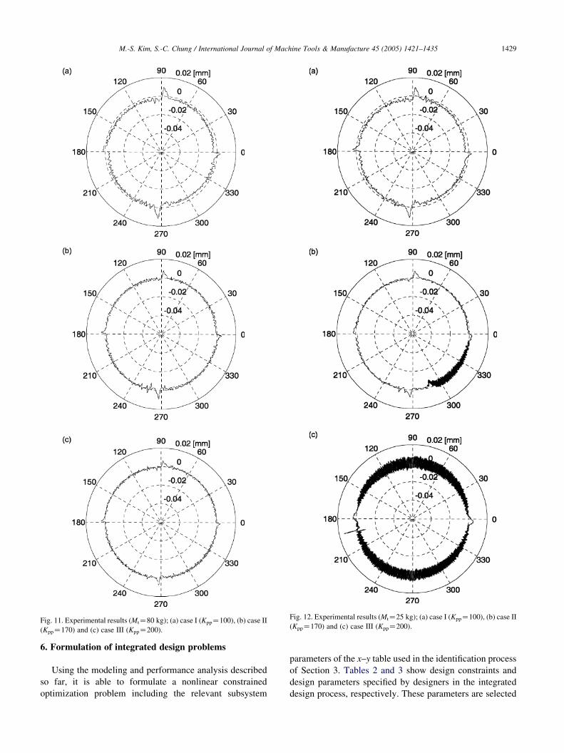
Fig. 11. Experimental results (MtZ80 kg); (a) case I (KppZ100), (b) case II

(KppZ170) and (c) case III (KppZ200).

Fig. 12. Experimental results (MtZ25 kg); (a) case I (KppZ100), (b) case II

(KppZ170) and (c) case III (KppZ200).


6. Formulation of integrated design problems

Using the modeling and performance analysis described

so far, it is able to formulate a nonlinear constrained

optimization problem including the relevant subsystem

parameters of the x–y table used in the identification process

of Section 3. Tables 2 and 3 show design constraints and

design parameters specified by designers in the integrated

design process, respectively. These parameters are selected


based on operating conditions of high-speed feed drive

systems [1,2].

Based on the integrated design methodology described in

Section 1, both mechanical and control parameters are

considered as the design variables x. Abbe offset, ballscrew

lead and diameter, as well as controller gains, Kff, Kpp, Kvp

and Kvi, of the 2-DOF controller are selected as the design

variables:

x Z ½Daa;Dbs; l; Kff ; Kpp; Kvp; Kvi�T (26)

Since interactions between mechanical and control

subsystems are considered simultaneously in design vari-

ables, a systematic design procedure is realized. Objectives

of the design procedure are minimization of the Abbe offset,

magnitude of the contour error ratio, the equivalent inertia

and the inverse of bandwidth of the feed drive system while

the related constraints are satisfied.

In usual optimization methods, only one evaluative

factor is considered as a single objective function, and

others are considered as constraint functions. However, in

such a method, complicated relationships among the

evaluative factors are difficult to investigate, and design

results derived from the single objective optimization do not

provide a comprehensive view of the system to designers.

Therefore, in order to overcome these disadvantages, a

multi-objective optimization method is introduced in which

several evaluative factors are adopted as objective

functions.

Optimal solutions of a multi-objective function have

been obtained by using a weighting method, a constraint

method, a non-inferior set estimation method and so on.

A weighting method is generally utilized owing to its

simplicity and physical meanings. In this paper, the

weighting method is applied to perform the integrated

design of the feed drive system. To solve the multi-objective

optimization problem numerically by using the weighting

method, it is converted into a sequence of scalar

optimization problems in which the objective function is

Table 2

Constraints for the integrated design

Constraint Equation

Maximum feedrateg1 : Vmax KVc !0; Vc Z

11:2Dbsl

pL2bs

ffis

Maximum deformationg2 : dc Kda !0; dc Z

b

2ke

2Ccos b

sin bBt

�Buckling load

g3 : Fxc KPb !0; Pb Z

4p2EbsIbs

L2bs

Nominal stability g4 : jzijK1!0; zi Zfz : DcðzÞZ0g;

Gain margin g5 : A�m KAm !0; Am Z20 log10½1=jG

Phase margin g6 : f�m Kfm !0; fm Z:½Goðe

jugTs Þ

Saturated torque g7 : tmaxc Ktmax

m !0; tmaxc Z maxfnjG

Saturated control inputg8 : t

maxm KTmax !0; t

maxm Z

Jeq

R

d2

dt2a

defined by a linear combination of all objective functions

with nonnegative different weighting factors. The objective

function OM of the multi-objective problem using the

weighting method is formulated as

OMðxÞ Z c1Daa Cc2Jeq Cc3jErjCc4

1

uB

(27)

where ck, kZ1–4 is the weighting factor of each objective

function.

Dimensionless variables are introduced in the design

process. Normalization of the multi-objective function

minimizes detrimental effects on design results, which are

induced by round-off errors and divergence in the

optimization process. Therefore, the normalized multi-

objective function OMN is represented as follows.

OMNðxÞ Z c1D�aa Cc2J�

eq Cc3E�r Cc4u�

B

D�aa Z

Daa

Daa0

; J�eq Z

Jeq

Jeq0

; E�r Z

Er

Er0

� �2

; u�B Z

uB0

uB

ð28Þ

where Daa0, Jeq0, Er0 and uB0 are initial values of Abbe

offset, equivalent inertia, contour error ratio and bandwidth

of the feed drive system. A multi-objective function renders

it possible to reflect various aims of designers through

the selection of weighting factors. Consequently, the

integrated design problem is formulated as the nonlinear

constrained optimization problem as follows:

Minimize

OMNðxÞ Z c1D�aa Cc2J�

eq Cc3E�r Cc4u�

B

Subject to

giðxÞ%0; i Z 1;.; 8 xLj %xj%xU

j ;

j Z 1;.; 7 x Z ½Daa;Dbs; l;Kff ;Kpp;Kvp;Kvi�T ð29Þ

where gi is the vector of inequality constraints, xLj and xU

j

are the lower and upper limits of design variables,

respectively.

ffiffiffiffiffiffiEbs

rbs

Btb Ccosh bBtb

b Csinh bBtb

�ðFz

c CFwÞ

iZ1–n

oðejupTs Þj�

�Cp

satðejuTs Þxcðe

juTs Þjg

max

Table 3

Design parameters specified by a designer

Design parameter Symbol (unit) Value

Torque constant of the motor Kt (N m/Arms) 0.498

Back-e.m.f. constant of the motor Kemf (Vrms/rpm) 0.0142

Maximum velocity of the motor umaxm (rpm) 5000

Maximum torque of the motor Tmax (N m) 3.82

Rotor inertia Jrt (kg m2) 0.173!10K4

Table width Wtb (m) 0.3

Table length Ltb (m) 0.3

Stroke Lst (m) 0.3

Circular radius Ri (m) 0.1

Circular velocity ui (rad/s) 5

Maximum acceleration amax (m/s2) 2 g

Maximum velocity Vmax (m/s) 0.75

Cutting force Fc (N) (100, 100, 100)

Load capacity Fw (N) 500

Allowable gain margin A�m (dB) 10

Allowable phase margin f�m (degree) 50

Allowable deformation error da (m) 5!10K6

Time constant of the I-controller ti (s) 0.01

Order of the closed-loop system n 7

Table 4

Integrated design results-design variables

Design variable Unit Initial system Integrated

design

x1 (Daa) m 0.060 0.043

x2 (Dbs) m 0.016 0.013

x3 (l) m 0.005 0.013

x4 (Kff) V/V 0.100 0.140

x5 (Kpp) V/V 100.000 98.672

x6 (Kvp) V/V 1.000 2.977

x7 (Kvi) V/V 0.100 0.397

Table 5

Integrated design results-system performances

Performance Unit Initial system Integrated

design

Er % 6.680 0.067

uB rad/s 12.717 40.030

Jeq kg m2 1.03!10K4 8.13!10K5

tmaxc N m 1.288 0.816


The Sequential Quadratic Programming (SQP) method

[17], which is suitable for nonlinear constrained optimiz-

ation problems, is employed to perform the integrated

design of the feed drive system. The SQP solves a nonlinear

function of the design variables by using a quadratic

approximation. The approximation is made of the Hessian

of the Lagrangian function using a quasi-Newton updating

method. This is then used to generate a QP subproblem

whose solution is used to form a search direction for a line

search procedure. The SQP algorithm is implemented by the

use of Optimization Toolbox in MATLAB [13]. Design

parameters of the x–y table that had been applied to the

identification process are used as initial values of the design

variables in the optimization process.
Am dB 38.773 25.201
fm degree 81.749 75.761

Fig. 13. Comparisons of bode diagrams of the closed-loop.

7. Results of integrated design problems

7.1. Results of the integrated design

Based on Tables 2 and 3, as well as Eq. (29), the

integrated design for the precision feed drive system in

which weighting factors of the multi-objective function are

set to have a uniform effect to the optimization process is

performed. Results of the integrated design are listed in

Tables 4 and 5. The initial system represented in Tables 4

and 5 and Figs. 13 and 14 means the x–y table that had been

applied to the identification process.

Figs. 13 and 14 show comparisons of Bode diagrams and

step responses of the closed-loop, respectively. The design

results not only satisfy all the constraints but also improve

the desired system performance.

From Tables 4 and 5, it confirms that the Abbe offset and

the contour error ratio are reduced. In addition, system

bandwidth is increased more than three times through

the integrated design. tmaxc in Table 5 means that required

motor power and the corresponding control input for the

designed feed drive system have been decreased owing to

the objective function that minimizes Abbe offset and

equivalent inertia, as well as the constraint of actuator

saturation. However, the relative stability is decreased as

shown in Table 5. This comes from the fact that controller

gains obtained from the integrated design process are larger

than those of the initial system. It means that the initial

mechanical subsystem has been over designed. It is

confirmed that the design results not only satisfy all the

constraints but also achieve the desired system performance.

The effectiveness of the integrated design methodology is

confirmed through the results.

Fig. 14. Comparisons of step responses.


7.2. Pareto optimum solutions

The objective functions considered in the integrated

design process interact mutually, and conflicting relation-

ships exist among them. For example, there exist conflicting

relationships between minimization of the Abbe offset and

maximization of the system bandwidth. In other words,

design changes for improving system accuracy cause

degradation of response characteristics of the feed drive

system. From this fact, for the integrated design of feed

drive systems, it is required to select proper design variables

according to which one gives a better result between the

accuracy and response characteristics.

A typical description of a Pareto optimum technique,

which is the determination of the compromise set of

multi-objective problems, has been proposed [7,8].

The conflicting relationships between the objective func-

tions are able to be evaluated by using the Pareto optimum

solution set. Pareto optimum solutions are obtained by using

the weighting method in which the sum of each weighting

factor is 1. The multi-objective function OP described in Eq.

(30), minimization of the Abbe offset and the inverse of

bandwidth, is considered in order to obtain the Pareto

optimum solution set as

Table 6

Design variables and objective functions of Pareto optimum solutions

No. Weighting factors

(W1/W2)

Design variables

x1 (Daa) x2 (Dbs) x3 (l) x4 (

1 0.1 0.9 0.026 0.006 0.026 0.10

2 0.2 0.8 0.027 0.007 0.024 0.06

3 0.3 0.7 0.027 0.007 0.024 0.07

4 0.4 0.6 0.027 0.006 0.023 0.10

5 0.5 0.5 0.028 0.007 0.020 0.22

6 0.6 0.4 0.029 0.008 0.019 0.14

7 0.7 0.3 0.030 0.008 0.019 0.09

8 0.8 0.2 0.033 0.009 0.015 1.21

9 0.9 0.1 0.041 0.016 0.011 0.07

OPðxÞ Z W1u�B CW2D�

aa (30)

where W1,2 is the weighting factor of each objective

function. Increase in the weighting factor W1 means that

the system bandwidth is considered as a more desirable

factor than the Abbe offset of the feed drive system. Pareto

optimum solutions are obtained according to different

weighting factors in the interval of [0, 1]. Table 6 shows

the optimal values of design variables and objective

functions according to various weighting factors.

As shown in Table 6, the optimal values of each

objective function have a trend according to the weighting

factors. As the weighting factor W1 is increased, the system

bandwidth and the Abbe offset are increased. The conflict-

ing relationships between two objective functions for the

feed drive system are presented in Figs. 15 and 16. The

optimum solutions along the curve from to in Fig. 15

are called the Pareto optimum solution set as.

Fig. 17 show mechanical and control design variables

of the Pareto optimum solution set. The design variables

are also changed according to the weighting factor. When

the weighting factor W1 is increased, velocity controller

gains and the ballscrew diameter are increased, and the

ballscrew lead is decreased to satisfy the desired

performance of the system response. However, it is

difficult to find a certain behavior in the position and

feedforward controller gains according to weighting

factors.

Pareto optimum results are very useful for the integrated

design of the feed drive system. For example, when

designers want to focus on increasing the system accuracy

rather than response characteristics of the feed drive

system, they can select points such as to on the

curve of Fig. 15 and then read the corresponding design

variables in Table 6. In addition, the Pareto optimum

solution set allows designers to quantize relationships

among objective functions and to determine the influence

of one objective function to the others. Although only

one design solution is chosen for the implementation, the

knowledge of relationships between the objective functions

provides the flexibility of the systematic design methodo-

logy substituting one solution for the other according to the

Objective functions

Kff) x5 (Kpp) x6 (Kvp) x7 (Kvi) u�B D�

aa

0 100.19 0.560 5.96!10K4 0.329 0.437

8 102.77 0.610 8.93!10K4 0.312 0.446

5 98.48 0.674 1.08!10K3 0.305 0.449

7 79.52 1.080 1.15!10K3 0.260 0.451

0 99.62 1.251 6.52!10K3 0.207 0.470

5 88.46 1.713 7.18!10K3 0.190 0.492

0 90.36 1.769 3.78!10K2 0.186 0.502

0 100.26 2.083 6.53!10K2 0.153 0.548

0 101.02 3.856 8.95!10K2 0.142 0.678

Fig. 15. Pareto optimum solution set.


required system performance. Therefore, formulation of

the integrated design of a feed drive system as a multi-

objective optimization problem and its Pareto optimum

solution set provide designers with a deeper understanding

about the interaction between mechanical and control

subsystems as well as the design optimization of a feed

drive system.

Fig. 17. Optimal values of design variables of the Pareto optimum set; (a)

mechanical design variables, (b) velocity controller gains and (c) position

and feedforward controller gains.

8. Conclusions

A systematic design methodology is proposed to

design a high-speed/precision feed drive system. In

addition to the strict modeling of subsystems, an accurate

identification process of the mechanical subsystem has

been conducted. Parametric studies and circular motion

experiments on the x–y table are performed in order to

investigate interactions between mechanical and control

subsystems, as well as the influence of the interactions

on system performance. From the circular motion

experiments, it is confirmed that limitations of system

performance depend on characteristics of both mechan-

ical and control subsystems.

Fig. 16. Optimal values of objective functions according to weighting

factors.

A multi-objective function and normalization technique

are introduced in the design process. According to the

simulation results of the case studies in the x–y table, the

system bandwidth is increased more than three times and

Abbe offset decreased by 28 percent through the proposed

design methodology.

The conflicting relationship between two objectives,

minimizing the Abbe offset and the inverse of the bandwidth

of the feed drive system, is investigated through the Pareto

optimum solution set. Contrary to a unique optimum

solution offered by optimization methods of a single

objective function, the versatility of optimization of

the feed drive system is obtained through the Pareto

optimum method.

Consequently, it is confirmed how controller gains and

mechanical design parameters are selected for the

optimal design and fabrication of feed drive systems.

Fig. A1. Elements of the mechanical subsystem element.


Developed design methodology gives not only the

possibility to evaluate and optimize the dynamic motion

performance of the feed drive system, but also improves the

quality of the design process to achieve the required

performance for high-precision/speed feed drive systems.

Appendix A. Dimensions and parameters of the

mechanical subsystem

Dimensions and parameters of the mechanical subsystem

used in this paper are listed as follows (Fig. A1):

Knt
nut stiffness (N/m)
Ksb
stiffness of a support bearing (N/m)
Lstr
stroke of a feed drive system (m)
Gcp
shear modulus of a coupling (Pa)
Dcp
coupling diameter (m)
Lcp
coupling length (m)
Ebs
elastic modulus of a ballscrew (Pa)
Gbs
shear modulus of a ballscrew (Pa)
Dbs
ballscrew diameter (m)
rbs
ballscrew density (kg/m2)
Ibs
moment of inertia of a ballscrew (m4)
Lbs
ballscrew length (m)
Etb
elastic modulus of a table (Pa)
rtb
table density (kg/m2)
Itb
moment of inertia of a table (m4)
Btb
table width (m)
Ltb
table length (m)
Elg
elastic modulus of a linear guide (Pa)
Ilg
moment of inertia of linear guides (m4)
Llg
length of a linear guide (m)
Lsp
distance between linear guides (m)
Fig. B1. A beam model on the elastic foundation.

Appendix B. Beams on elastic foundations

We assume that Ilg is constant during design procedures.

And dimensions of linear guides are dependent on table

dimensions and stroke of a feed drive system as follows

(Fig. B1):

Lsp Z2

3Btb; Llg Z 2Lstr (B.1)

From Ref. [16], the spring constant ke of linear guides on

elastic foundation is given by

ke Z48ElgIlg

LspL3lg

Z48ElgIlg

23

Btbð2LstrÞ3

Z9ElgIlg

BtbL3str

(B.2)

Therefore, the deformation error of a mechanical

structure in the vertical direction is described as follows:

dc Zb

2ke

2 Ccos bBtb Ccosh bBtb

sin bBtb Csinh bBtb

� �ðFz

c CFwÞ;

b Zke

4EtbItb

� �1=4(B.3)

Moment of inertia of the table Itb is calculated as

Itb ZLtbH3

tb

12(B.4)


From Eqs. (B.2)–(B.4),

b

2ke

Z1

64EtbItbk3e

� �1=4

ZBtbL3

str

18ElgIlg

27ElgIlg

EtbLtbBtbL3strH

3E

� �1=4

(B.5)

From the definition of Abbe offset in Section 4, the height

of a table Htb can be represented in terms of Abbe offset Daa

and ballscrew diameter Dbs as follows:

Daa Z 2Da Z 2Htb CDbs; Htb ZDaa KDbs

2(B.6)

Therefore, the deformation error of a mechanical

structure in the vertical direction including the Abbe offset

Daa is described as follows:

dc ZBtbL3

str

3ElgIlg

ElgIlg

6EtbLtbBtbL3strðDaa KDbsÞ

3

� �1=4

!2 Ccos bBtb Ccosh bBtb

sin bBtb Csinh bBtb

� �ðFz

c CFwÞ ðB.7)

References

[1] J. Tlusty, High-speed machining, Annals of the CIRP 42 (2) (1993)

733–738.

[2] A. Miles, High Performance Machining, Hanser Gardner Publication,

Cincinnati, 1998.

[3] Y. Koren, Control of machine tools, Transactions on ASME Journal of

Manufacturing Science and Engineering 199 (1997) 749–755.

[4] M. Ebrahimi, R. Whalley, Analysis, modeling and simulation of

stiffness in machine tool drives, Computers and Industrial Engineer-

ing 38 (2000) 93–105.

[5] A. Dequidt, J.M. Castelain, E. Valdes, Mechanical pre-design of high

performance motion servomechanisms, Mechanism and Machine

Theory 35 (2000) 1047–1063.

[6] Y. Kakino, A. Matsubara, Z. Li, D. Ueda, H. Nakagawa, T. Takeshita,

H. Maruyama, A study on the total tuning of feed drive systems in NC

machine tools (4th report), Journal of the JSPE 63 (3) (1997) 368–372

(in Japanese).

[7] J. Koski, Multicriterion optimization in structural design, in: New

Directions in Optimum Structural Design, Wiley, New York, 1984.

[8] M. Yoshimura, T. Hamada, K. Yura, K. Hitomi, Multi-objective

design optimization of machine-tool spindles, Transactions of the

ASME, Journal of Mechanisms, Transmissions, and Automation in

Design 106 (1984) 46–53.

[9] LM System Catalog—Technical Reports, THK Co., Ltd, 1992.

[10] E. Kaan, Y. Altintas, High speed CNC system design. Part I—jerk

limited trajectory generation and quintic spline interpolation,

International Journal of Machine Tools and Manufacture 41 (2001)

1323–1345.

[11] L. Ljung, System Identification-Theory for the User, Prentice Hall

PTR, New Jersey, 1999.

[12] M.S. Kim, S.C. Chung, Identification of nonlinear characteristics for

precision servomechanisms, in: Proceedings of ASPE Annual Meet-

ing Portland, 26–31 Oct., 2003, pp. 167–170.

[13] MATLAB User Guide, Mathworks, Inc., 2000.

[14] H. Nakazawa, Principles of precision engineering, Oxford University

Press, New York, 1994.

[15] B.C. Kuo, Digital Control System, Saunders College Publishing,

Florida, 1992.

[16] A.C. Ugural, S.K. Fenster, Advance Strength and Applied Elasticity,

Elsevier, New York, 1987.

[17] J.S. Arora, Introduction to Optimum Design, McGraw-Hill, Inc.,

Singapore, 1989.

a systematic approach to design high-performance feed drive systems

Documents