a survey of stackelberg differential game models in …aprasad/stackelbergreview.pdf · a survey of...

J Syst Sci Syst Eng (Dec 2007) 16(4): 385-413 ISSN: 1004-3756 (Paper) 1861-9576 (Online) DOI: 10.1007/s11518-007-5058-2 CN11-2983/N

© Systems Engineering Society of China & Springer-Verlag 2007

A SURVEY OF STACKELBERG DIFFERENTIAL GAME MODELS IN SUPPLY AND MARKETING CHANNELS

Xiuli HE1 Ashutosh PRASAD1 Suresh P. SETHI1 Genaro J. GUTIERREZ2 1School of Management, The University of Texas at Dallas, Richardson, TX 75080

[email protected], [email protected], [email protected] ( ) 2McCombs School of Business, The University of Texas at Austin, Austin, TX 78731

[email protected]

Abstract

Stackelberg differential game models have been used to study sequential decision making in

noncooperative games in diverse fields. In this paper, we survey recent applications of Stackelberg

differential game models to the supply chain management and marketing channels literatures. A

common feature of these applications is the specification of the game structure: a decentralized channel

composed of a manufacturer and independent retailers, and a sequential decision procedure with

demand and supply dynamics and coordination issues. In supply chain management, Stackelberg

differential games have been used to investigate inventory issues, wholesale and retail pricing

strategies, and outsourcing in dynamic environments. The underlying demand typically has growth

dynamics or seasonal variation. In marketing, Stackelberg differential games have been used to model

cooperative advertising programs, store brand and national brand advertising strategies, shelf space

allocation, and pricing and advertising decisions. The demand dynamics are usually extensions of the

classical advertising capital models or sales-advertising response models. We begin by explaining the

Stackelberg differential game solution methodology and then provide a description of the models and

results reported in the literature.

Keywords: Stackelberg differential games, supply chain management, marketing channels, open-loop

equilibria, feedback policies, channel coordination, optimal control

1. Introduction The study of differential games was initiated

by Isaacs (1965) with applications to warfare

and pursuit-evasion problems. Since then,

differential game models have been used

extensively to study problems of conflict arising

in such diverse disciplines as operations

management, marketing, and economics.

Particularly related to our review are

applications of differential games in supply

chain management and marketing channels. A

number of books and papers have surveyed

applications in these areas (e.g., Jørgensen 1982,

Feichtinger et al. 1994, Dockner et al. 2000,

Erickson 1992, 1995, 1997). However, all of

these surveyed applications consist of duopoly

A Survey of Stakelberg Differential Game Models in Supply and Marketing Channels

JOURNAL OF SYSTEMS SCIENCE AND SYSTEMS ENGINEERING 386

and oligopoly situations in which the decisions

are made simultaneously, and the objective is to

obtain Nash equilibrium solutions.

More recently, differential games have been

formulated to study the hierarchical or

sequential decision making situations that exist

in supply chains and marketing channels, and for

which a reasonable solution concept is that of

Stackelberg equilibrium (Stackelberg 1952).

Stackelberg differential game (SDG) models

have been used to study conflicts and

coordination issues associated with inventory

and production policies, outsourcing, capacity

and shelf space allocation decisions, dynamic

competitive advertising strategies, and pricing

for new products. It is these studies that we shall

survey in this paper.

It should be noted at the outset that the

literatures on supply chain and marketing

channels management are closely related, since

both deal with physical delivery of the product

from suppliers to end users through

intermediaries and in the most efficient manner.

However, the supply chain literature has been

more concerned with production quantity and

inventory decisions, and demand uncertainty,

whereas marketing papers have looked at pricing

and promotions decisions, customer

heterogeneity, and brand positioning.

Competition and channel coordination are

important issues in both. Since these topics are

rapidly converging, we will therefore provide a

combined overview in this paper.

In supply chain management, Stackelberg

differential games have been applied to the study

of topics such as inventory and production

issues, wholesale and retail pricing strategies,

and outsourcing in dynamic environments. The

underlying demand may have growth dynamics

or seasonal variation. In the marketing area, we

discuss applications such as cooperative

advertising programs, shelf space allocation, and

price and advertising decisions. The demand

dynamics are usually advertising capital models

(e.g., Nerlove and Arrow 1962) or

sales-advertising response models (e.g.,

Vidale-Wolfe 1957 and Sethi 1983). In the

former, advertising is considered as an

investment in the stock of goodwill and, in the

latter, sales-advertising response is specified as a

direct relation between the rate of change in

sales and advertising.

The fact that the papers that have applied

SDG models to supply and marketing channels

problems are relatively few in number and

recent, suggests that the literature is still at a

formative stage. Although, over the last two

decades, supply chain management as a whole

has garnered much research attention, most

studies of strategic interactions between the

channel members are based on the static

newsvendor framework. By static, we mean that

although these models may have two stages, one

where the leader moves and the second where

the follower moves, thereby modeling sequential

decision making in the channel, they overlook

strategic issues that arise when the firms interact

with each other repeatedly over time and make

decisions in a dynamic fashion. We therefore

hope that this survey, by focusing on dynamic

interactions between the channel members,

generates further interest in this emerging area

of research.

We shall limit the scope of our survey to

applications using differential games, i.e., where

the strategies are in continuous time with a finite

HE, PRASAD, SETHI and GUTIERREZ


or infinite horizon, and where the Stackelberg

equilibrium is the solution concept. Thus, we

exclude from its purview dynamic games played

in discrete time. We also do not review

applications in economics, for which we refer

the interested readers to Bagchi (1984).

This paper is organized as follows. In

Section 2, we introduce the concepts and

methodology of Stackelberg differential games.

In Section 3, we review SDG models in the area

of supply chain management. In Section 4, we

discuss their applications to marketing channels.

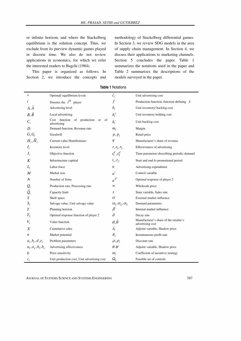
Section 5 concludes the paper. Table 1

summarizes the notations used in the paper and

Table 2 summarizes the descriptions of the

models surveyed in the paper.

Table 1 Notations

* Optimal/ equilibrium levels ic Unit advertising cost

i Denotes the thi player f Production function, function defining x&

ˆ,A A Advertising level ih Unit inventory/ backlog cost

ˆ,B B Local advertising ih+ Unit inventory holding cost

iC Cost function of production or of advertising ih− Unit backlog cost

D Demand function, Revenue rate im Margin

, iG G Goodwill , ip p Retail price

,i iH H Current-value Hamiltonians q Manufacturer’s share of revenue

iI Inventory level 1 2, ,r r r Effectiveness of advertising

iJ Objective function 1 2,d dt t Time paremeters describing periodic demand

K Infrastructure captital ,s ft t Start and end fo promotional period

iL Labor force u Advertising expenditure

M Market size iu Control variable

N Number of firms 02u Optimal response of player 2

iQ Production rate, Processing rate w Wholesale price

iQ Capacity limit x State variable, Sales rate

S Shelf space α External market influence

iS Salvage value, Unit salvage value 1 2 3, ,α α α Demand parameters

T Planning horizon β Internal market influence

2T Optimal response function of player 2 δ Decay rate

iV Value function ˆ,θ θ Manufacturer’s share of the retailer’s advertising cost

X Cumulative sales iλ Adjoint variable, Shadow price

a Market potential iπ Instantaneous profit rate

, , ,i i ia b d e Problem parameters , iρ ρ Discount rate

, , ,l s l sa a b b Advertising effectiveness ,φ ψ Adjoint variable, Shadow price

b Price sensitivity iω Coefficient of incentive strategy

ic Unit production cost, Unit advertising cost iΩ Feasible set of controls



Table 2 Summary of model description

Paper Dynamics L’s decisions F’s decisions Solution1

Breton, Jarrar, and Zaccour (2006) Lanchester type Ad. effort Ad. effort FSE

Chintagunta and Jain (1992) NA dynamics Ad. effort Ad. effort OLNE

Desai (1992) Seasonal Production rate, Price Price OLSE

Desai (1996) Seasonal Production rate, Price Price OLNE, OLSE

Eliashberg and Steinberg (1987) Seasonal Production rate, Price Price OLSE

Gutierrez and He (2007) Bass type Price Price OLSE

He, Prasad, and Sethi (2007) Sethi 1983 Participation rate, Price Ad. Effort, Price FSE

He and Sethi (2008) Bass type Price Price OLSE

Jain and Chintagunta (2002) NA dynamics Ad. Effort, Price Ad. Effort, Price OLNE, FNE

JSZ (2000)2 NA dynamics Participation rate, Ad. Effort Ad. effort FNE, FSE

JSZ (2001)2 NA dynamics Ad. Effort, Price Ad. Effort, Price FNE, FSE

JTZ (2003)3 NA dynamics Participation rate, Ad. Effort Ad. Effort, Price FSE

JTZ (2006)3 NA dynamics Ad. effort Ad. effort FSE

Karray and Zaccour (2005) NA dynamics Ad. Effort, (coop), Price Ad. Effort, Price FSE

Kogan and Tapiero (2006) General Price Price OLNE, OLSE

Kogan and Tapiero (2007a) General Price, Production rate Price OLSE

Kogan and Tapiero (2007b) General Processing rate Production rate OLSE

Kogan and Tapiero (2007c) General Price Order quantity OLSE

Kogan and Tapiero (2007d) General Price Order quantity OLSE

Kogan and Tapiero (2007e) General Price Price OLSE

Martin-Herran and Taboubi (2005) NA dynamics Ad. Effort, Incentive Shelf-space FNE, FSE

1The symbol OLNE = Open-loop Nash equilibrium, FNE = Feedback Nash equilibrium, OLSE =

Open-loop Stackelberg equilibrium, and FSE = Feedback Stackelberg equilibrium. 2JSZ is the abbreviation for Jørgensen, Sigue, and Zacccour. 3JTZ is the abbreviation for Jørgensen, Taboubi, and Zaccour.

2. Basics of the Stackelberg Differential Game A differential game has the following

structure: 1) The state of the dynamic system at

any time t is characterized by a set of variables

called the state variables. Typical state variables

are market share, sales, inventory, goodwill, etc.

2) There are decision variables called controls



that are chosen by the game players: For

example, order quantity, pricing, advertising,

and shelf-space decisions etc. 3) The evolution

of the state variables over time is described by a

set of differential equations involving both state

and control variables. 4) Each player has an

objective function (e.g., the present value of the

profit stream over time) that it seeks to

maximize by its choice of decisions.

There are several different concepts of

equilibria in differential games. In this paper, we

are concerned with SDG models. Like the static

Stackelberg game, due originally to Stackelberg

(1952), an SDG is hierarchical (or sequential) in

nature. We consider an SDG involving two

players labeled as 1 (the leader) and 2 (the

follower) making decisions over a finite horizon

T . We shall also remark on what needs to be

done when T = ∞ . Let ( ) nx t R∈ denote the

vector of state variables, 111

mu R∈Ω ⊂ denote

the control vector of the leader, and 22

2mu R∈Ω ⊂ denote the control vector of the

follower. The sequence of the play is as follows.

The leader announces its control path 1( )u ⋅ .

Then, the follower decides its optimal control

path 2 ( )u ⋅ in response to the announced 1( )u ⋅ .

A Stackelberg equilibrium is obtained when the

leader solves its problem taking into account the

optimal response of the follower.

Further specification is required in terms of

the information structure of the players in order

to precisely define a Stackelberg equilibrium. In

this section, we shall consider two different

information structures. The first one, called the

open-loop information structure, assumes that

the players must formulate their decisions at

time t only with the knowledge of the initial

condition of the state at time zero. The second

one, called the feedback information structure,

assumes that the players use their knowledge of

the current state at time t in order to formulate

their decisions at time t . We give the procedure

for obtaining an open-loop solution in Section

2.1. The feedback solution procedure will be

described in Section 2.2.

2.1 Open-Loop Solution The solution procedure is that of backward

induction. That is, like the leader, we first

anticipate the follower’s best response to any

announced policy of the leader. The anticipation

is derived from solving the optimization

problem of the follower given the leader’s policy.

We then substitute the follower’s response

function into the leader’s problem and solve for

the leader’s optimal policy. This policy of the

leader, together with the retailer’s best response

to that policy, constitutes a Stackelberg

equilibrium of the SDG. For the open-loop

solution, given an announced decision 1 1( ) ( ( ) 0 )u u t t T⋅ = , ≤ ≤ by the leader, the

follower’s optimal control problem is

2

2 12 0

( )max[ ( ( ) ( ))u

J t x u u⋅

, , ⋅ ; ⋅

2 1 220( ( ) ( ) ( ))

T te t x t u t u t dtρ π−= , , ,∫

22 ( ( ))]Te S x Tρ−+

subject to the state equation

1 2( ) ( ( ) ( ) ( ))x t f t x t u t u t= , , , ,& 0(0)x x= , (1)

where 2 0ρ > is the follower’s discount rate,

2π is its instantaneous profit rate function,

2 ( ( ))S x T is the salvage value, and 0x is the

initial state. Recall that the open-loop

information structure for both players means that

the controls 1( )u t and 2 ( )u t at time t depend



only on the initial state 0x . We assume

that 1 2( )f t u u, ⋅, , , 1 22 ( )t u uπ ,⋅, , , and 2 ( )S ⋅ are

continuously differentiable on [0 ]nR t T,∀ ∈ , .

Let 02 ( )u ⋅ denote the follower’s optimal

response to the announced control 1( )u ⋅ by the

leader. The optimal response of the follower

must be made at time zero and will, in general,

depend on the entire announced control path 1( )u ⋅ by the leader and the initial state 0x .

Clearly, given 1( )u ⋅ , which can be expressed as

a function of 0x and t, the follower’s problem

reduces to a standard optimal control problem.

This problem is solved by using the maximum

principle (see e.g., Sethi and Thompson 2000),

which requires introducing an adjoint variable or

a shadow price that decouples the optimization

problem over the interval [0 ]T, into a sequence

of static optimization problems, one for each

instant [0 ]t T∈ , . Note also that the shadow

price at time t denotes the per unit value of a

change in the state ( )x t at time t, and the

change ( )x t& in the state at time t requires only

the time t control 1( )u t from the leader’s

announced control trajectory 1( ).u ⋅ Neverthe-

less, we shall see later that the follower’s

optimal response 02 ( )u t at any given time t

will depend on the entire 1( )u ⋅ via the solution

of the two-boundary problem resulting from the

application of the maximum principle. Let us

now proceed to solve the follower’s problem

given 1( )u ⋅ .

The follower’s current-value Hamiltonian is

1 22 ( )H t x u uλ, , , ,

1 2 1 22 ( ) ' ( )t x u u f t x u uπ λ= , , , + , , , , (2)

where nRλ ∈ is the (column) vector of the

shadow prices associated with the state variable

x , the (row) vector 'λ denotes its transpose,

and it satisfies the adjoint equation

1 22

2

' ' ( )

'( ) ( ( ))

H t x u ux

T S x Tx

λ ρλ λ

λ

∂= − , , , , ,∂

∂= .∂

&

(3)

Here we have suppressed the argument t as is

standard in the control theory literature, and we

will do this whenever convenient and when

there arises no confusion in doing so. Note that

the gradient 2H x∂ /∂ is a row vector by

convention.

The necessary condition for the follower’s

optimal response denoted by 02u is that it

maximizes 2H with respect to 22u ∈Ω , i.e.,

0

22

2 1 22( ) arg max ( ( ) ( ) ( ) )

uu t H t t x t u t uλ

∈Ω= , , , , . (4)

Clearly, it is a function that depends on t , x ,

λ , and 1u . A usual procedure is to obtain an

optimal response function 12 ( )T t x uλ, , , so that

02 ( )u t 2T= 1( ( ) ( ) ( ))t x t t u tλ, , , . In the case when 02 ( )u t is an interior solution, 2T satisfies the

first-order condition

12 22( ) 0H t x u T

uλ∂ , , , , = .

∂ (5)

If the Hamiltonian 2H defined in (2) is jointly

concave in the variables x and 2u for any

given 1,u then the condition (5) is also

sufficient for the optimality of the response 2T

for the given 1u .

It is now possible to complete our discussion

of the dependence of the follower’s optimal

response 2T on 1( )u ⋅ and 0x . Note that the

time t response of the follower is given by

02 12( ) ( ( ) ( ) ( ))u t T t x t t u tλ= , , , . (6)

But the resulting two-point boundary value



problem given by (1), (2) with 12 ( )T t x uλ, , , in

place of 2u makes it clear that the shadow price

( )tλ at time t depends on the entire 1( )u ⋅ and

0x . Thus, we have the dependence of 02 ( )u t ,

and therefore of 02 ( )u ⋅ , on 1( )u ⋅ and 0x .

If we can explicitly solve for the optimal

response 12 ( )T t x uλ, , , , then we can specify the

leader’s problem to be

1( )maxu ⋅

11[ ( ( ))J t x u, , ⋅

1 1 11 20( ( ))

T te t x u T t x u dtρ π λ−= , , , , , ,∫

11( ( ))]Te S x Tρ−+ , (7)

1 12( ( ))x f t x u T t x uλ= , , , , , , ,& 0(0)x x= , (8)

1 12 2 2

2

' ' ( ( ))

'( ) ( ( ))

H t x u T t x ux

T S x Tx

λ ρ λ λ λ

λ

∂= − , , , , , , , ,∂

∂= ,∂

&

(9)

where 1 0ρ > is the leader’s discount rate and

the differential equations in (8) and (9) are

obtained by substituting the follower’s best

response 12 ( )T t x uλ, , , for 2u in the state

equation (1) and the adjoint equation (3),

respectively. We formulate the leader’s

Hamiltonian

11( )t x uH λ φ ψ, , , , ,

= 1 11 2( ( ))t x u T t x uπ λ, , , , , ,

1 12' ( ( ))f t x u T t x uφ λ+ , , , , , ,

1 12 2'[ ( ( ( ))) ']H t x u T t x u

xψ ρλ λ λ∂+ − , , , , , , , ,

∂

(10)

where nRφ ∈ and nRψ ∈ are the vectors of

the shadow prices associated with x and λ ,

respectively, and they satisfy the adjoint

equations

1 11 21' ' ( ( ))t x u T t x uH

xφ ρ φ λ φ ψ λ∂= − , , , , , , , , ,

∂&

1 11 1 2

1 12

' ( ( ))

' ( ( ))

t x u T t x ux

f t x u T t x ux

ρ φ π λ

φ λ

∂= − , , , , , ,∂

∂− , , , , , ,∂

21 1

2 22

2

1 22

' ( ( ))

'( ) ( ( )) ( ( )) ( )

H t x u T t x ux

T S x T S x T Tx x

ψ λ λ

φ ψ

∂+ , , , , , , , ,∂

∂ ∂= − ,∂ ∂

(11)

1 11 21' ' ( ( ))t x u T t x uHψ ρψ λ φ ψ λ

λ∂= − , , , , , , , , ,∂

&

1 11 1 2

1 12

' ( ( ))

' ( ( ))

t x u T t x u

f t x u T t x u

ρψ π λλ

φ λλ

∂= − , , , , , ,∂

∂− , , , , , ,∂

21 1

2 22' ( ( ))H t x u T t x u

xψ λ λ∂+ , , , , , , , ,

∂

(0) 0ψ = . (12)

In (10), we are using the notation 1H for

the Hamiltonian to recognize that it uses the

optimal response function of the follower for 2u in its definition. In (11) and (12), we have

used the envelope theorem (see, e.g., Derzko et

al. 1984 ) in taking the derivative 1 xH∂ /∂ .

Finally, it is important to remark that unlike

in Nash differential game, the adjoint equation

and the transversality condition ( )Tφ′ in (11)

have a second-order term each on account of the

facts that the adjoint equation (9) is a state

equation in the leader’s problem and that it has a

state-dependent terminal condition, also in (9),

arising from the sequential game structure of

SDG. The necessary optimality condition for the

leader’s optimal control 1 ( )u t∗ is that it



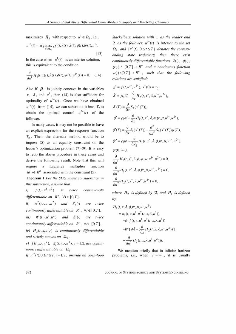
maximizes 1H with respect to 11u ∈Ω , i.e.,

11

1 11( ) arg max ( ( ) ( ) ( ) ( ) )

uu t t x t t t t uH λ φ ψ∗

∈Ω= , , , , , .

(13)

In the case when 1( )u t is an interior solution, this is equivalent to the condition

111( ( ) ( ) ( ) ( ) ( )) 0t x t t t t u tH

uλ φ ψ ∗∂ , , , , , = .

∂ (14)

Also if 1H is jointly concave in the variables

x , λ , and 1u , then (14) is also sufficient for

optimality of 1 ( )u t∗ . Once we have obtained 1 ( )u t∗ from (14), we can substitute it into 2T to

obtain the optimal control 2 ( )u t∗ of the

follower.

In many cases, it may not be possible to have

an explicit expression for the response function

2T . Then, the alternate method would be to

impose (5) as an equality constraint on the

leader’s optimization problem (7)-(9). It is easy

to redo the above procedure in these cases and

derive the following result. Note that this will

require a Lagrange multiplier function

( ) nRµ ⋅ ∈ associated with the constraint (5).

Theorem 1 For the SDG under consideration in

this subsection, assume that

i) 1 2( )f t u u, ⋅, , is twice continuously

differentiable on [0 ]nR t T, ∀ ∈ , .

ii) 2 1 2( )t u uπ ,⋅, , and 2 ( )S ⋅ are twice

continuously differentiable on [0 ]nR t T, ∀ ∈ , .

iii) 1 1 2( )t u uπ ,⋅, , and 1( )S ⋅ are twice

continuously differentiable on [0 ]nR t T, ∀ ∈ , .

iv) 12 ( )H t x u, , , ⋅ is continuously differentiable

and strictly convex on 2Ω .

v) 2( ),f t x u, ,⋅, 2( ) 1 2,i t x u iπ , ,⋅, , = , are contin-

uously differentiable on 1Ω .

If ( ) 0 1 2iu t t T i∗ , ≤ ≤ , = , , provide an open-loop

Stackelberg solution with 1 as the leader and

2 as the follower, 1 ( )u t∗ is interior to the set

iΩ , and ( ) 0 x t t T∗ , ≤ ≤ denotes the corresp-

onding state trajectory, then there exist

continuously differentiable functions ( )λ ⋅ , ( )φ ⋅ ,

( )ψ ⋅ : [0 ] nT R, → and a continuous function

( ) [0 ] nT Rµ ⋅ : , → , such that the following

relations are satisfied:

1 20( ) (0)f t u u x xx

∗ ∗ ∗∗ = , , , = ,&

1 22 2 ( )H t x u u

xλ ρ λ λ∗ ∗ ∗∂′ ′= − , , , , ,

∂&

2( ) ( ( ))T S x Tx

λ ∗∂′ = ,∂

1 21 1( )H t x u u

xφ ρ φ λ φ ψ µ∗ ∗ ∗∂′ ′= − , , , , , , , ,

∂&

2

1 22( ) ( ( )) ( ( )) ( )T S x T S x T T

x xφ ψ∗ ∗∂ ∂′ = − ,

∂ ∂

1 21 1

2

' ( )H t x u uψ ρψ λ φ ψ µλ

∗ ∗ ∗∂′ = − , , , , , , , ,∂

&

(0) 0ψ = ,

1 211( ) 0H t x u u

uλ φ ψ µ∗ ∗ ∗∂ , , , , , , , = ,

∂

1 212( ) 0H t x u u

uλ φ ψ µ∗ ∗ ∗∂ , , , , , , , = ,

∂

1 222( ) 0H t x u u

uλ∗ ∗ ∗∂ , , , , = ,

∂

where 2H is defined by (2) and 1H is defined

by

1 21( )H t x u uλ φ ψ µ, , , , , , ,

1 2 11( ( ))t x u u t x uπ λ= , , , , , ,

1 2 1' ( ( ))f t x u u t x uφ λ+ , , , , , ,

1 22'[ ( ( )) ']H t x u u

xψ ρλ λ∂+ − , , , ,

∂

1 222( )H t x u u

uλ µ∂+ , , , , .

∂

We mention briefly that in infinite horizon problems, i.e., when T = ∞ , it is usually



assumed that the salvage values 1 2 0S S= = .

Then the practice is to replace the terminal conditions on ,λ φ and ψ by

2lim ( ) 0T

Te Tρ λ−

→∞= , 1lim ( ) 0T

Te Tρ φ−

→∞= , and

1lim ( ) 0T

Te Tρ ψ−

→∞= , respectively. We should

note that these conditions are not necessary, but

are sufficient when coupled with appropriate

concavity conditions.

It is known that in general open-loop

Stackelberg equilibria are time inconsistent. This

means that given an opportunity to revise its

strategy at any future time after the initial time,

the leader would benefit by choosing another

strategy than the one it chose at the initial time.

Thus, an open-loop Stackelberg equilibrium only

makes sense if the leader can credibly

pre-commit at time zero its strategy for the

entire duration of the game. In many

management settings such commitment is not

observed in practice. Nevertheless, there is a

considerable literature dealing with open-loop

Stackelberg equilibria, on account of their

mathematical tractability.

2.2 Feedback Solution In the preceding section, we have described

an open-loop Stackelberg solution concept to

solve the SDG. We shall now develop the

procedure to obtain a feedback Stackelberg

solution. While open-loop solutions are said to

be static in the sense that decisions can be

derived at the initial time, without regard to the

state variable evolution beyond that time,

feedback equilibrium strategies at any time t

are functions of the values of the state variables

at that time. They are perfect state-space

equilibria because the necessary optimality

conditions are required to hold for all values of

the state variables, and not just the values that lie

on the optimal state-space trajectories. Therefore,

the solutions obtained continue to remain

optimal at each instant of the time after the game

has begun. Thus, they are known as subgame

perfect because they do not depend on the initial

conditions.

Since differential games evolve in

continuous time, it is worthwhile to elaborate on

the physical interpretation of their sequential

move order. A feedback Stackelberg solution to

an SDG can be conceptualized as the limit of the

feedback Stackelberg solutions of a sequence of

discrete-time dynamic games, each one obtained

by time discretization of the original differential

game, with ( 1)stk + game in the sequence

corresponding to a finer discretization than the thk one. Each of these games can be termed as

a “sampled-state” game, as the only time

discretization is in the information set

comprising the state vector. Furthermore, as

explained in Basar and Olsder (1999), the

feedback Stackelberg solution of each

state-sampled game can be obtained by solving a

sequence of approximately defined open-loop

Stackelberg games. Consequently, the limiting

solution involves solutions of a sequence of

open-loop Stackelberg games, each one defined

on an infinitesimally small sub-interval, which

means that we now must obtain Stackelberg

solutions based on the incremental profit at each

time t.

Let ( )iV t x, denote the feedback Stackelberg

profits-to-go of player i in current-value term

at time t, at state .x For any given policy 1( )u t x, by the leader, the follower’s HJB

equation is



22 2

( )V t xV

tρ ∂ ,−

∂

2 2

1 22 ( )max ( ( ) )u

V t xf t x u t x u

x∈Ω

∂ ,= , , , ,∂

1 22 ( ( ) ),t x u t x uπ+ , , , , (15)

with 2 2( , ) ( ).V T x S x= The follower’s

instantaneous reaction function is given by

1 22 ( )

VT t x u

x

∂, , ,∂

22

1 22arg max[ ( )u

Vf t x u u

x∈Ω

∂= , , ,

∂

1 22 ( )]t x u uπ+ , , , . (16)

Given this, the leader’s HJB equation can be

written as

11 1

( )V t xV

tρ ∂ ,−

∂

11

1 2 1 21max [ ( ( ))

u

Vt x u T t x u

xπ

∈Ω

∂= , , , , , ,

∂

1 11 22

( )( ( ))],

V t x Vf t x u T t x u

x x

∂ , ∂+ , , , , , ,∂ ∂

(17)

with 1 1( , ) ( ).V T x S x= Maximizing the right-

hand side of (17) yields the optimal feedback

pricing for the leader, i.e., 1 ( )u t x∗ ,

11

1 2 1 21arg max[ ( ( ))

u

Vt x u T t x u

xπ

∈Ω

∂= , , , , , ,

∂

1 11 22( ( ))]

V Vf t x u T t x u

x x

∂ ∂+ , , , , , , .∂ ∂

(18)

Then, the optimal control policy for the follower

is obtained by substituting 1 ( )u t x∗ , for 1u in

(16), i.e.,

2 1 22( ) ( ( ) )

Vu t x T t x u t x

x∗ ∗ ∂, = , , , , .

∂ (19)

Substituting (18) and (19) into (15) and (17),

we can rewrite the HJB equation for the game as

the system

11 1

( )V t xV

tρ ∂ ,−

∂

1 21( ( ) ( ))t x u t x u t xπ ∗ ∗= , , , , ,

1 21( )( ( ) ( ))

V t xf t x u t x u t x

x∗ ∗∂ ,+ , , , , , ,

∂

22 2

( )V t xV

tρ ∂ ,−

∂

1 22 ( ( ) ( ))t x u t x u t xπ ∗ ∗= , , , , ,

1 22 ( )( ( ) ( ))

V t xf t x u t x u t x

x∗ ∗∂ ,+ , , , , , ,

∂

( ) ( ) 1 2i iV T x S x i, = , = , .

This system can be solved to obtain 1( )V t x,

and 2 ( )V t x, , and the feedback Stackelberg

strategies 1 ( )u t x∗ , and 2 ( )u t x∗ , .

3. Supply Chain Management Applications In this section we shall review applications

in the supply chain management area. The leader

is the supplier or manufacturer who decides on

variables such as the wholesale price and/or

production rate, whereas the retailer is the

follower and its decision variables can be, for

example, retail price and shelf-space allocation.

3.1 Eliashberg and Steinberg (1987): Pricing and Production with Constant Wholesale Price The paper by Eliashberg and Steinberg (1987)

considers a decentralized assembly system

composed of a manufacturer and a distributor.

The distributor processes the product and its

demand has seasonal fluctuations. As an aside,

Pekelman (1974) used a general time-varying

demand function ( ) ( ) ( ) ( )D t a t b t p t= − , where

( )a t is the market potential, ( )b t is the

coefficient of price sensitivity, and ( )p t is the

distributor’s price. In Eliashberg and Steinberg



(1987), it is assumed that ( )b t is constant and

( )a t has the form 21 2 3( )a t t tα α α= − + + ,

0 t T≤ ≤ , where 1α , 2α and 3α are positive

parameters and 2 1T α α= / .

The manufacturer and the distributor play an

SDG with the manufacturer as the leader and the

retailer as the follower. The distributor

determines its processing, pricing, and inventory

policies. The manufacturer decides its

production rate and a constant wholesale price.

The distributor’s problem is

0( ) ( )max [ ( ) ( ) ( )

R

T

R RI p

J p t D t wQ t⋅ , ⋅

= −∫

( ( )) ( )] R R R RC Q t h I t dt− − ,

( ) ( ) ( )RR t Q t D tI = − ,&

(0) ( ) 0 ( ) 0R R RI I T I t= = , ≥ ,

where ( )RQ t is its processing rate, ( )R RC Q is

its processing cost function, Rh is its inventory

holding cost per unit, and ( )RI t is its inventory

level. Similar to Pekelman (1974), a linear

holding cost function is used. It is assumed that

the processing cost function is increasing and

strictly convex.

The paper shows that the distributor follows

a two-part processing strategy. During the first

part of the processing schedule, it processes at a

constant increasing rate. This policy builds up

inventory initially and then draws down

inventory until it reaches zero at a time Rt∗ .

During the second part, which begins at the

stockless point Rt∗ , it processes at precisely the

market demand rate. Pricing also follows a

two-part strategy. The price charged by the

distributor is first increasing at a decreasing rate

and then decreasing at an increasing rate. The

inventory builds up for a while and then reaches

zero. From then on, the distributor processes just

enough to meet demand.

An intuitive interpretation is as follows. The

distributor, facing a seasonal demand that

increases and then decreases, can smooth out

processing operations by carrying inventory

initially due to the assumption of convex

processing cost. In other words, if it did not

carry any inventory throughout the entire

horizon, it could incur higher costs due to the

convexity of the processing cost function.

Turning to the manufacturer’s problem, let

M M MQ I h, , , and ( )M MC Q denote its

production rate, inventory level, inventory

holding cost per unit, and the production cost

function, respectively. The manufacturer’s

problem is given by

0( )max [( ) ( )M

T

M M RQ w

J w c Q w t⋅ ,

= − ,∫

( ( )) ( )] M M M MC Q t h I t dt− − ,

( ) ( ) ( )M RM t Q t Q w tI = − , ,&

(0) ( ) 0M MI I T= = ,

( ) ( ) 0 ( ) 0M R MQ t Q t I t≥ ≥ , ≥ ,

where Mc is its cost per unit transferred to the

distributor and ( )RQ w t, is the best response of

the distributor at time t given w . It is assumed that Mw c> and that the production cost

function is quadratic.

The manufacturer’s policies are character-

ized as following a two-part production policy.

During the first part, it produces at a constantly

increasing rate. During the second part, which

begins at the manufacturer’s stockless point Mt∗ ,

it produces at exactly the distributor’s

processing rate. In general, if the manufacturer’s

inventory holding cost per unit is sufficiently



low and the distributor’s processing efficiency

and inventory holding cost per unit are high,

then the manufacturer can also smooth out its

operations.

3.2 Desai (1992): Pricing and Production with Retailer Carrying No Inventory Desai (1992) analyzes the production and

pricing decisions in a channel composed of a

manufacturer that produces the goods and sells

them through a retailer who serves the final

market. This paper differs from Eliashberg and

Steinberg (1987) in three ways. First, it allows

the manufacturer to change the wholesale price

over time. Second, the retailer is not allowed to

carry inventory. Third, a quadratic holding cost

function is assumed. The retailer faces a

price-dependent seasonal demand. As in

Eliashberg and Steinberg (1987), Desai (1992)

uses a time varying demand function ( )D t =

( ) ( ),a t bp t− where 1( )a t α= + 2 sin( )t Tα π /

and T is the duration of the season. The retailer

(the follower) decides on the pricing policy, and

its problem is given by

0( )max[ [ ( ) ( )] ( ) ]

T

Rp

J p t w t D t dt⋅

= − ,∫

where ( )p t is the retail price and ( )w t is the

wholesale price charged by the manufacturer.

Note that Eliashberg and Steinberg assumed the

wholesale price to be constant. Here, the

manufacturer (the leader) decides on the

wholesale price ( )w t and its production rate

( )MQ t . Its problem is

2

0( ) ( )max [ [ ( ) ( ) ( )

M

T

M M Mw Q

J w t D t c Q t⋅ , ⋅

= −∫

2 ( )] ( )]M M M Mh I t dt S I T− + ,

where Mh is the inventory holding cost, Mc is

the per unit production cost, ( )MI t is the

inventory level at time t , and MS is the per

unit salvage value. The inventory dynamics is

( ) ( ) ( )MMM

dIt Q t D tI

dt= = − ,& 0(0)M MI I= ,

where ( ) 0MQ t ≥ and ( ) 0D t ≥ .

The result is that once the production rate

becomes positive, it does not become zero again,

which implies production smoothing. However,

none of the gains of production smoothing are

passed on to the retailer. The optimal production

rate and the inventory policy are a linear

combination of the nominal demand rate, the

peak demand factor, the salvage value, and the

initial inventory. In the scenario where the

retailing operation does not require an effort, the

pricing policies of the manufacturer and the

retailer and the production policy of the

manufacturer have the synergistic effect that an

increase in the manufacturer’s price or

production rate or the retailer’s price leads to an

increase in the rate of change of inventory.

However, in the scenario where the retailing

operation does benefit from the effort, the

retailer’s pricing policy may not necessarily be

synergistic with the other policies.

3.3 Desai (1996): Pricing and Production with Further Processing by the Retailer This paper extends Desai (1992) by requiring

the retailer to process the goods received from

the manufacturer before they can be sold in the

final market. The manufacturer makes the

production and pricing decisions while the

retailer decides on the processing rate and



pricing policies. The paper considers optimal

policies under three types of contracts: contracts

under which the manufacturer charges a constant

price throughout a season, contracts under which

the retailer processes at a constant rate

throughout the season, and contracts under

which the manufacturer and retailer cooperate to

make decisions jointly. It is shown that the type

of contract does not significantly impact the

retailer’s price. However, the type of contract

has an impact on the manufacturer’s price and

the production rate as well as the retailer’s

processing rate. If the demand is not highly

seasonal, a constant processing rate contract will

lead to higher production and processing rates,

and a lower manufacturer’s price compared to a

constant manufacturer’s price contract.

3.4 Gutierrez and He (2007): Life-Cycle Channel Coordination Gutierrez and He (2007) study the

intertemporal channel coordination issues in an

innovative durable product (IDP) supply chain

composed of a manufacturer who produces the

IDP and a retailer who serves the final market.

The demand in all the above papers has

seasonal variations which are exogenously

determined and independent of the retail price.

Therefore, there is no interdependence between

the demand in different periods. In contrast, the

demand in this paper evolves according to a

Bass (1969) type diffusion process. Specifically,

the demand is affected by the external and

internal market influences (i.e., word-of-mouth)

as well as the retail price. The word-of-mouth

creates an interdependence between the current

and future demand.

The manufacturer is the leader and

announces the wholesale price trajectory. The

retailer follows by deciding on the retail price

trajectory. While the manufacturer is far-sighted,

i.e., it maximizes its life-cycle profits, two

possibilities for the retailer are considered: (1) a

far-sighted strategy of maximizing the life-cycle

profit, and (2) a myopic strategy of maximizing

the instantaneous profit rate at any time t . They

address the following research questions: Does

the manufacturer prefer the retailer to be

far-sighted or myopic? Does the retailer prefer to

be far-sighted or myopic? They derive open-loop

pricing strategies for both players.

Far-sighted Retailer. When the retailer is

far-sighted, for a given wholesale price path

( )w ⋅ , it chooses in response a retail price path

( )p ⋅ by solving the problem

0( )max [ ( ) ( ) ] ( )

T

Rp

p t w t c X t dt⋅

− −∫ & (20)

0

( ) ( ( ))( ( ))(1 ( ))

(0)

X t M X t X t bp t

X X

α β= − + − ,= ,

& (21)

where Rc is the per unit selling cost including

any opportunity cost, α and β are internal

and external influence parameters, b is the price sensitivity parameter, and 0X is the initial

number of adopters. The manufacturer’s problem is

0( )max [ ( ) ] ( )

T

Mw

w t c X t dt⋅

− ,∫ & (22)

0

1( ) ( ( ))1 [ ( ) ( )]

2(0)

R RX t F X t b w t c t

X X

λ= − + − ,

= ,

& (23)

1( ) [ 2 ( )]

4R t M X tb

α β βλ = − − + −& •

21 [ ( ) ( )] ,R Rb w t c tλ− + − ( ) 0R Tλ = ,

(24)



where Mc is the per unit production cost and

Rλ is the retailer’s shadow price. Note that X

and Rλ are the manufacturer’s two state

variables, and their evolution incorporates the

retailer’s best response.

Myopic Retailer. For each [0 ]t T∈ , , the

retailer selects its response ( )p t in order to

maximize its instantaneous profit rate at time t

subject to the state equation (21). Accordingly,

we remove the retailer’s shadow price Rλ from

the retailer’s best response and then obtain the

manufacturer’s optimization problem as (22) and

(23) with ( )R tλ removed from (23).

The paper finds that the manufacturer does

not always find it more profitable for the retailer

to be far-sighted, and may sometimes be better

off if the retailer is myopic. On the other hand

both the manufacturer and the retailer are better

off if the retailer is far-sighted when the final

market is insufficiently penetrated. However, if

the market is close to saturation such as at the

end of the planning horizon, the manufacturer

will shift its preference and be better off with a

myopic retailer, while the retailer prefers to be

far-sighted. However, monitoring the retailer

sales volume or retail price becomes an

implementation necessity when the

manufacturer offers a wholesale price contract

assuming the retailer is myopic.

3.5 He and Sethi (2008): Pricing and Slotting Decisions He and Sethi (2008) extend the work of

Gutierrez and He (2007) by considering the

impact of shelf space allocation (or another

promotional device for that matter) on retail

demand. Here it is assumed that retail demand is

a concave increasing function of the shelf-space

of merchandise displayed on the shelf. This is

operationalized by introducing a multiplicative

term ( )S t to the right-hand side of (21),

where ( )S t is the shelf space allocated to the

product at time t , and by including a linear cost

of shelf space in the retailer’s objective function

(20). The solution is for the equilibrium

wholesale and retail pricing and slotting

decisions. However, in connection with the

strategic profitability foci of the retailer, myopic

or far-sighted, the obtained results are similar to

those in Gutierrez and He (2007).

3.6 Kogan and Tapiero (2007a): Inventory Game with Endogenous Demand This paper considers a supply chain

consisting of a manufacturer (leader) and a

retailer (follower) facing a time-dependent

endogenous demand depending on the price set

by the retailer. Furthermore, the retailer has a

finite processing capacity, which requires

consideration of the effect of inventory. Thus,

the retailer must decide on the retail price ( )p t

as well as the order quantity ( )RQ t . The

manufacturer, on the other hand, has ample

capacity and must decide on only the wholesale

price ( )w t . It is assumed that the game is

played over a season of length T which

includes a short promotional period [ ]s ft t,

such as the Christmas time, during which both

the demand potential ( )a t and the customer

price sensitivity ( )b t are high. Specifically, the

demand ( ) ( ) ( ) ( )D t a t b t p t= − , where

1

2

( ),

s f

s f

a t t and t ta t

a t t t

, < ≥⎧⎪= ⎨ , ≤ <⎪⎩



1

2

( ),

s f

s f

b t t and t tb t

b t t t

, < ≥⎧⎪= ⎨ , ≤ <⎪⎩

with 2 1a a> and 2 1b b> . The manufacturer is

assumed to be restricted to setting a constant

wholesale price 1w in the regular periods and

2 1w w≤ in the promotion period. The

manufacturer has ample capacity and produces

exactly according to the retailer’s order to

maximize its profit:

0( )max [ ( ) ( ) ( )]

T

R M Rw

w t Q t c Q t dt⋅

−∫

subject to ( ) Mw t c≥ , where Mc is the per unit

production cost.

The retailer’s selects its order quantity

( )RQ t and the retail price ( )p t , 0 t T≤ < , by

solving the problem:

0( ) ( )max ( )[ ( ) ( ) ( )]R

T

Q pp t a t b t p t

⋅ , ⋅−∫

( ) ( ) ( ) ( ( ))R R Rc Q t w t Q t h X t dt− − − ,

( ) ( ) [ ( ) ( ) ( )]RR t Q t a t b t p tI = − − ,&

0 ( )RQ t Q≤ ≤ ; ( ) ( ) ( ) 0 ( ) 0a t b t p t p t− ≥ ; ≥ ,

where Q is the retailer’s maximum processing

rate.

The optimal solution to the centralized

problem as well as the Stackelberg equilibrium

is obtained. The analysis requires the system to

begin in a steady state at time 0 , go to a

transient state in response to promotional

decisions, and then revert back to the steady

state by the end of the season at time T. Thus,

the solution is meant to be implemented in a

rolling horizon fashion.

Under reasonable conditions on the

parameters, formulas for the equilibrium values

of the regular and promotional wholesale prices

for the manufacturer are derived. It is shown that

it is beneficial for the retailer to change pricing

and processing policies in response to the

reduced promotional wholesale price and the

increased customer price sensitivity during the

promotion. The change is characterized by

instantaneous jump upward in quantities ordered

and downward in retailer prices at the instant

when the promotion period starts and vice versa

just when the promotion ends. In fact, the

retailer starts lowering its prices sometime

before the promotion starts. This causes a

greater demand when the promotion period

begins, thereby taking advantage of the reduced

wholesale price during the promotion. This is

accomplished gradually to strike a trade-off

between the surplus/backlog cost and the

wholesale price over time. Specifically, any

reduction in the wholesale price results first in

backlog and then in surplus. An opposite

scenario takes place on the side when the

promotion periods end.

In the symmetric case when unit backlog and

surplus costs are equal, the typical equilibrium

as shown in Figure 1 is obtained. As can be seen,

due to symmetric costs, the transient solution is

symmetric with respect to the midpoint of the

promotion phase.

Finally, due to inventory dynamics, the

traditional two-part tariff does not coordinate the

supply chain as it does in the static case. This is

because the manufacturer when setting the

promotional wholesale price ignores not only the

retailer’s profit margin from sales, but also the

profit margin from handling inventories.

However, in the special case where the

manufacturer fixes a wholesale price throughout

the season, the retailer’s problem becomes

identical to the centralized problem and the

supply chain is coordinated.



Figure 1 Optimal policies with promotion

3.7 Kogan and Tapiero (2007b): Inventory Game with Exogenous Demand This game differs from Kogan and Tapiero

(2007a) in two ways. First, the demand is no

longer price-dependent, and so pricing is not an

issue. This simplifies the problem. Second, both

the manufacturer and the retailer have limited

capacities in contrast to the previous game in

which only the retailer has a limited capacity.

The objective of each member is to decide on

the production/processing rates that minimize

inventory costs over an infinite planning horizon.

This paper assumes that the retailer is the leader

who decides on the order quantity. Let Rh+ , Mh+ ,

Rh− , Mh− be the retailer’s inventory holding cost,

the manufacturer’s inventory holding cost, the

retailer’s backlog cost, and the manufacturer’s

shortage cost per unit, respectively. Let

max 0R RI I+ = , and max 0R RI I− = − , . The

retailer’s objective is to find a production rate

RQ in order to minimize its all inventory related

costs. Let ( ( )) ( ) ( )R R R R R Rh I t h I t h I t+ + − −= + denote

its total inventory cost at time t . Its problem is

given by

( )min ( ( ))f

sR

t

R RtQh I t dt

⋅,∫

( ) ( ) ( ) 0 ( )R RR Rt Q t D t Q t QI = − , ≤ ≤ ,&

where RI is the retailer’s inventory level, RQ

is the retailer’s processing rate, RQ is the

maximum processing rate, and ( )D t is a

step-wise and periodic customer demand rate for

the product given as

1 2

2 1

( )

1 2 ,

( 1) 1 2 ,

d dR

d dM

D t

d t jT t t JT jQ

d t j T t t JT jQ

=

⎧ > , + < ≤ + , = , ...⎪⎨⎪ < , + − < ≤ + , = , ...⎩

where MQ is the manufacturer’s production

limit. The manufacturer’s problem is



( )min ( ( )) min ( ( ))f f

s sM M

t t

M M M Mt tQ Qh I t dt h I t dt

⋅=∫ ∫

( ) ( ) ( ) 0 ( )M R MM Mt Q t Q t Q t QI = − , ≤ ≤ ,&

where ( ( )) ( ) ( )M M M M M Mh I t h I t h I t+ + − −= + is the

manufacturer’s inventory cost at time t .

For the centralized channel, if the retailer’s

backlog cost is lower than the manufacturer’s,

i.e., R Mh h− −< , and the retailer’s holding cost is

higher than the manufacturer’s, i.e., R Mh h+ +> ,

( M R M Rh h h h+ − − +≠ , ≠ ), then there is no backlog on

the manufacturer’s side. For the decentralized

channel in which the manufacturer is the leader,

the retailer processes products at the maximum

rate when it has an inventory surplus; when

there is a shortage, the retailer reduces the

processing rate to equal the maximum

production rate of the manufacturer. This

complicates the ordering decisions which

require multiple switching points induced by

coordinating inventory decisions and capacity

limitation. While the demand is not

price-dependent, it varies with time. Thus, the

optimal control problems faced by each of the

players is a standard dynamic inventory problem

as discussed, e.g., by Bensoussan et al. (1974).

Since production control appears linearly in

these problems, the optimal production policy

can have three possible regimes: maximum

production, (singular) production on demand,

and zero production. Sequencing of these

regimes depends on the time-varying nature of

the demand and inventory cost parameters.

As for coordination, the authors show that if

the retailer pays the manufacturer for its

inventory related cost, then the centralized

solution is attained. They also show that a

two-part tariff contract can be obtained to

coordinate the supply chain.

3.8 Kogan and Tapiero (2007c): Production Balancing with Subcontracting This paper considers a supply chain

consisting of one manufacturer (follower) and

one supplier (leader). The supplier has ample

capacity and so the inventory dynamics is not an

issue. The manufacturer, on the other hand, has a

limited capacity, and its decisions depend on the

available inventory. The product demand rate at

time t is ( )a t D% , where D% is a random

variable and ( )a t is known as the demand

shape parameter. The realization of D% is

observed only at the end of a short selling

season, such as in the case of fashion goods, and

as a result, the manufacturer can only place an

advance order to obtain an initial end-product

inventory, which is then used to balance

production over time with the limited in-house

capacity.

Thus, the problem is a dynamic version of

the newsvendor problem which incorporates

production control. The supplier’s problem is to

set a constant wholesale price to maximize its

profit from the advance order from the

manufacturer. The manufacturer must decide on

the advance order as well as the production rate

over time in order to minimize its total expected

cost of production, inventory/backlog, and

advance order. The authors show that it is

possible to transform this problem into a

deterministic optimal control problem that can

be solved to obtain the manufacturer’s best

response to the supplier’s announced wholesale

price.

The paper assumes that the unit in-house



production cost is greater than the supplier’s

cost , and shows that if the supplier makes profit

(i.e., has a positive margin), then the

manufacturer produces more in-house and buys

less than in the centralized solution. This is due

to the double marginalization not unlike in the

static newsvendor problem. Furthermore, if the

manufacturer is myopic, it also orders less than

the centralized solution even though it does not

produce in-house, since it does not take into

account the inventory dynamics.

While the optimal production rate over time

would depend on the nature of the demand, it is

clear that the optimal production policy will

have intervals of zero production, maximum

production, and a singular level of production.

The authors also solve a numerical example and

obtain the equilibrium wholesale price, the

manufacturer’s advance order quantity, and the

production rate over time.

3.9 Kogan and Tapiero (2007d): Outsourcing Game This paper considers a supply chain

consisting of one producer and multiple

suppliers, all with limited production capacities.

The suppliers are the leaders and set their

wholesale prices over time to maximize profits.

Following this, the producer decides on its

in-house production rate and supplements this

by ordering from a selection of suppliers over

time in order to meet a random demand at the

end of a planning period T. The producer incurs

a penalty for any unmet demand. Unlike in

Kogan and Tapiero (2007c), no assumption

regarding the cost of in-house production and

the supplier’s production cost is made here. The

producer’s goal is to minimize its expected cost.

As in Kogan and Tapiero (2007c), it is

possible to transform the producer’s problem

into a deterministic optimal control problem.

Because the producer’s problem is linear in its

decisions, the production rate has one of three

regimes as in the previous model, and its

ordering rate from any chosen supplier will also

have similar three regimes.

The authors show that the greater the

wholesale price of a supplier, the longer the

producer waits before ordering from that

supplier. This is because the producer has an

advantage over that supplier, up to and until a

breakeven point in time for outsourcing to this

supplier is reached. As in Kogan and Tapiero

(2007c), here also when a supplier sets its

wholesale price strictly above its cost over the

entire horizon, then the outsourcing order

quantity is less than that in the centralized

solution.

Again, the supply chain is coordinated if the

suppliers set their wholesale prices equal to their

unit costs and get lump-sum transfers from the

producer.

3.10 Kogan and Tapiero (2007e): Pricing Game

This paper concerns an SDG between a

supplier (the leader) who chooses a wholesale

price for a product and a retailer (the follower)

who responds with a retail product price. The

authors incorporate learning on the part of the

supplier whose production cost declines as more

units are produced. The demand for the product

is assumed to be decreasing in the retail price.

The authors show that myopic pricing is optimal

for the retailer. Under a certain profitability

condition, the retail price is greater than in the



centralized solution because of double

marginalization. However, the gap is larger than

that in the static pricing game. This is because

the higher retail price implies less cost reduction

learning in the dynamic setting in comparison to

that in the centralized solution, whereas in the

static framework no learning is involved in the

centralized solution and in the Stackelberg

solution.

3.11 Kogan and Tapiero (2007f): Co-Investment in Supply Chains

This paper considers a supply chain with N firms. Let ( )K t denote the current level of the

supply chain infrastructure capital,

1( ,..., )NL L L= denote a vector of the labor

force, 1( ,..., )NI I I= denote a vector of

investment policy, and ( )j jQ f K L= , denote

an aggregate production function of the thj

firm, where 0,fK∂ ≥∂

0j

fL∂ >∂ for 0,L ≠

( 0)0

j

f KL

∂ , = ,∂ and 2

20

j

fL

∂ <∂

. The process of

capital accumulation is given by

1( ) ( ) ( )

N

jj

K t K t I tδ=

= − + ,∑&0(0)K K= ,

( ( ) ( )) ( ) 0 1,..., .j jf K t L t I t j N, ≥ ≥ , =

The j th firm’s objective is to maximize its

discounted total profit, i.e.,

0( ) ( )max [ ( ) ( ( ) ( ))j

j j

tj j

L Ie p t f K t L t

ρ∞ −

⋅ , ⋅,∫

( ) ( ) ((1 ) ( ))] j j I jc t L t C I t dtθ− − − , 1 ,j N= ,... ,

where jp is the price, jc is the unit labor cost,

( )IC ⋅ is the investment cost function, and θ is

the portion of the cost that is subsidized.

The authors derive the Nash strategy as well

as the Stackelberg strategy for the supply chain

where firms are centralized and controlled by a

"supply chain manager". Their results show that

the Stackelberg strategy applied to consecutive

subsets of firms will result in an equilibrium

identical to that obtained in case of a Nash

supply chain. The implication is that it does not

matter who the leader is and who the followers

are.

4. Marketing Channel Applications Research in marketing has applied

differential game models to study dynamic

advertising strategies in competitive markets.

These papers mainly focus on the horizontal

interactions such as the advertising competition

between brands, and accordingly seek Nash

equilibria (Deal 1979, Deal et al. 1979, Teng and

Thompson 1983, Erickson 1992, Chintagunta

and Jain 1992, Fruchter and Kalish 1997).

Recently, a few SDG models have appeared

that study the vertical interaction in marketing

channels. In terms of their dynamics, these can

be categorized into two groups, advertising

capital models and sales-advertising response

models. Advertising capital models consider

advertising as an investment in the stock of

goodwill ( )G t as in the model of Nerlove and

Arrow (1962) (NA, thereafter). The advertising

capital is affected by the current and past

advertising expenditures by a firm on the

demand for its products. It changes over time

according to

0( ) ( ) ( ) (0) 0G t A t G t G Gδ= − , = ≥ ,& (25)

where ( )A t is the current advertising

investment (in dollars) and δ is a constant

positive decay rate.



Sales-advertising response models

characterize a direct relation between the rate of

change in sales and advertising. The

Vidale-Wolfe (1957) (VW, hereafter) advertising

model is given by

( )( ) ( )(1 ( )) ( )

dx tx t rA t x t x t

dtδ= = − − ,& 0(0)x x= ,

where x is the market share, A is the advertising

rate, and r is the effectiveness of advertising.

The Sethi (1983) model is a variation of the VW

model, and it is given by

( ) ( ) 1 ( ) ( )x t rA t x t x tδ= − − ,& 0(0)x x= . (26)

Sethi (1983) also gave a stochastic extension of

his model. Little (1979) discusses some of the

desirable features of the advertising models that

have appeared in the literature.

4.1 Jørgensen, Sigue, and Zaccour (2000): Dynamic Cooperative Advertising This paper studies a channel in which the

manufacturer and retailer can make advertising

expenditures that have both long-term and

short-term impacts on the retail demand.

Specifically, the long-term advertising affects

the carry-over effect of advertising, while the

short term advertising influences current retail

sales only.

The manufacturer controls its rate of

long-term advertising effort ( )A t and

short-term advertising effort ˆ( )A t . The retailer

controls its long-term advertising rate ( )B t and

short-term advertising rate ˆ ( )B t . An extended

NA model describes the dynamics of the

goodwill as

( ) ( ) ( ) ( )l lG t a A t b B t G tδ= + − ,&0(0)G G= ,

(27)

where la and lb are positive parameters that

capture the effectiveness of the long-term

advertising of the manufacturer and the retailer,

respectively. At any instant of time, the demand

D is given by

ˆ ˆˆ ˆ( ) ( )S SD A B G a A b B G, , = + ,

where Sa and Sb are parameters that capture

the effectiveness of the manufacturer’s and

retailer’s short-term advertising, respectively.

Suppose the manufacturer and the retailer

can enter into a cooperative advertising program

in which the manufacturer pays a certain share

of the retailer’s advertising expenditure. The

manufacturer is the Stackelberg game leader in

designing the program. It announces its

advertising strategies and support rates for the

retailer’s long-term and short-term advertising

efforts.

The manufacturer’s problem is

2

0ˆ ˆ( ) ( ) ,

1max [ ( )

2t

M M MA A

J e m D c A tρ

θ θ

−

⋅ , ⋅ ,= −∫

2 21 1ˆˆ ( ) ( ) ( )2 2 RMc t t c B tA θ− −

21 ˆ ˆ ˆ( ) ( ) ( ) ]2 Rt c t t dtBθ−

and the retailer’s is

0ˆ( ) ( )max [ t

R RB B

J e m Dρ−

⋅ , ⋅= ∫

21(1 ( )) ( )

2 Rt c B tθ− −

21 ˆ ˆ(1 ( )) ( ) ( ) ]2 Rt c t t dtBθ− − ,

where Rm and Mm are the manufacturer’s and

the retailer’s margins, respectively, ( )tθ and ˆ( )tθ are the percentages that the manufacturer

pays of the retailer’s long-term and short-term

advertising costs, respectively.

The results show that both the manufacturer



and the retailer prefer full support to either of

long-term or short-term support alone, which in

turn is preferred to no support at all.

4.2 Jørgensen, Sigue, and Zaccour (2001) : Impact of Leadership on Channel Efficiency This paper studies the effects of strategic

interactions in both pricing and advertising in a

channel consisting of a manufacturer and a

retailer. It considers three scenarios: the

manufacturer and retailer simultaneously choose

their margins and advertising rates; sequential

with the retailer as the leader; and sequential

with the manufacturer as the leader. The

manufacturer controls its margin ( )Mm t and

the rate of advertising ( )A t . The retailer

controls its margin ( )Rm t and the advertising

rate ( )B t . The demand rate ( )D t follows a NA

type of dynamics, and is given by

( ) ( )( ( )) ( )D t B t a bp t G t= − ,

where ( )p t is the retail price, a and b are

positive parameters, and ( )G t is the stock of

brand goodwill given by (27). It is assumed that

the retailer is myopic, meaning that it is only

concerned with the short-term effects of its

pricing and advertising decisions. The

manufacturer is concerned with its brand image.

The manufacturer's total profit is

0[ ( ) ( ( )) ( )t

M MJ e m t B a bp t G tρ∞ −= −∫

21( )]

2 Mc A t dt−


0[ ( ) ( )( ( )) ( )t

R RJ e m t B t a bp t G tρ∞ −= −∫

21( )]

2 Rc B t dt−

The authors show that the manufacturer’s

leadership and the retailer’s leadership in a

channel are not symmetric as in pure pricing

games. The manufacturer’s leadership improves

channel efficiency and is desirable in terms of

consumer welfare, but the retailer’s leadership is

not desirable for channel efficiency and for

consumer welfare.

4.3 Karray and Zaccour (2005): Advertising for National and Store Brands This paper considers a marketing channel

composed of a national manufacturer and a

retailer who sells the manufacturer’s national

product (labeled as 1 ) and may also introduce a

private label (denoted as 2 ) at a lower price

than the manufacturer’s brand. The paper finds

that while the retailer is better off by introducing

the private label, the manufacturer is worse off.

Furthermore, it investigates whether a

cooperative advertising program could help the

manufacturer to alleviate the negative impact of

the private label.

The manufacturer decides on the national

advertising ( )A t . The retailer controls the

promotion efforts 1( )B t for the national brand

and efforts 2 ( )B t for the store brand. The

retailer’s effort has an immediate impact on

sales, but they do not affect the dynamics of the

goodwill of the national brand. The goodwill

( )G t of the national brand evolves according to

the NA dynamics given by equation (25). The

demand functions 1D for the national brand and

2D for the store brand are as follows:

21 1 2 1 1 2 1( )D B B G aB b B e G dG, , = − + − ,

2 1 2 2 2 1 2( )D B B G aB b B e G, , = − − ,



where a , 1b , 2b , 1e , 2e , and d are positive

parameters.

Karray and Zaccour consider three scenarios:

1) Game N : The retailer carries only the

national brand (labeled as 1 ) and no cooperative

advertising program. It is shown that the retailer

promotes the national brand at a positive

constant rate and the advertising strategy is

decreasing in the goodwill.

2) Game S : The retailer offers both a store

brand and the national brand and there is no

cooperative advertising program. It is shown

that the retailer will promote the national brand

if the marginal revenue from doing so exceeds

the marginal loss on the store brand.

3) Game C : The retailer offers both brands

and the manufacturer proposes to the retailer a

cooperative advertising program. Here the

retailer will always promote the store brand. The

retailer will also promote the national brand, but

only under certain conditions specified in the

paper.

The conclusion is that the introduction of

store brand always hurts the manufacturer. The

cooperative advertising program is profit

Pareto-improving for both players.

4.4 Jørgensen, Taboubi, and Zaccour (2003): Retail Promotions with Negative Brand Image Effects In this paper, the manufacturer advertises in

the national media to build up the image for its

brand. The retailer locally promotes the brand

(by such means as local store displays and

advertising in local newspapers) to increase

sales revenue, but these local promotional efforts

are assumed to be harmful to the brand image.

This paper analyzes two firms in a cooperative

program in which the manufacturer supports the

retailer’s promotional efforts by paying part of

the cost incurred by the retailer when promoting

the brand. The two firms play an SDG where the

manufacturer is the leader. The paper addresses

the question of whether the cooperative

promotion program is profitable and whether the

retailer’s decision on being a myopic or

far-sighted will affect the implementation of a

cooperative program.

Let ( )A t , ( )B t , and ( )G t denote the

manufacturer’s advertising rate, the retailer’s

promotional rate, and the brand image,

respectively. The dynamics of ( )G t is described

by the differential equation

( ) ( ) ( ) ( )G t aA t bB t G tδ= − − ,&0(0) 0G G= > ,

where a and b are positive parameters

measuring the impact of the manufacturer’s

advertising and retailer’s promotion, respectively,

on the brand image. The margin on the product

is ( ( ) ( )) ( ) ( )m B t G t dB t eG t, = + , where d and

e are positive parameters that represent the

effects of promotion and brand image on the

current sales revenue. With this formulation of

the demand and the revenue, the retailer faces a

trade-off between the sales volume and the

negative impact of the local advertising on the

brand image.

The manufacturer and the retailer incur

quadratic advertising and promotional costs 2( ( )) 2AC A t c A= / and 2( ( )) 2,BC B t c B= /

respectively. The manufacturer’s objective

functional is

0 [ ( ) ( )]t

MJ e q dB t eG tρ∞ −= +∫

2 2( ) ( ) ( )

2 2A Bc A t c t B t

dtθ

− −




0 (1 )[ ( ) ( )]t

RJ e q dB t eG tρ∞ −= − +∫

2(1 ( )) ( )

2Bc t B t

dtθ−

− ,

where q is the manufacturer’s fraction of the

margin and ( )tθ is the fraction the

manufacturer contributes to the retailer’s

promotion cost.

It is shown that a cooperative program is

implementable if the initial value of the brand

image 0G is sufficiently small, and if the initial

brand image is “intermediate” but promotion is

not “too damaging” (i.e., b is small) to the

brand image.

4.5 Martin-Herran and Taboubi (2005): Shelf-space Allocation

This paper considers a supply chain with one

retailer and two manufacturers. The retailer has

limited shelf-space and must decide on the

allocation of the shelf-space to the two products.

Let 1( )S t denote the fraction of the shelf-space

allocated to product i, 1 2,i∈ , then

2 1( ) 1 ( )S t S t= − . At time t , each manufacturer

i decides on its advertising strategy ( )iA t and

a shelf-space dependent display allowance

( ) ( ) ( ),i i iW t t S tω= where ( )i tω is the

coefficient of the incentive strategy. The retail

demand is a function of the shelf-space and

goodwill given by

1( ) ( )[ ( ) ( )]

2i i i i i iD t S t a G t b S t= − ,

where iG is the goodwill for brand i evolving

according to the NA dynamics. This model

implies that the shelf-space has a diminishing

marginal effect on the sales.

The paper assumes that the retailer and two

manufacturers play an SDG game with the

retailer as the follower, while the two

manufacturers play a Nash game, i.e., they

announce simultaneously their advertising and

incentive strategies 1ω and 2ω .

The authors show that manufacturers can

affect the retailer’s shelf-space allocation

decisions through the use of incentive strategies

(push) and/or advertising investment (pull).

Depending on the system parameters, the

manufacturer should choose between incentive

strategies and/or advertising.

4.6 Jørgensen, Taboubi, and Zaccour (2006): Incentives for Retail Promotions This paper considers a channel composed of

a manufacturer selling a particular brand to the

retailer. The manufacturer invests in national

advertising, which improves the image of its

brand, while the retailer makes local promotions

for the brand. The manufacturer and the retailer

play an SDG with the manufacturer as the leader.

The dynamics of the goodwill stock follows the

classical NA dynamics given in (25). Jørgensen

et al. (2006) assume that the manufacturer and

retailer apportion a fixed share of the total

revenue. They consider two scenarios: joint

maximization and individual maximization.

They show that the manufacturer advertises

more in the joint maximization scenario than

under individual maximization. This result does

not depend on whether or not the manufacturer

supports the retailer’s promotion in the

individual maximization case.



4.7 Breton, Jarrar, and Zaccour (2006): Feedback Stackelberg Equilibrium with a Lanchester-Type Model and Empirical Application

This paper studies dynamic equilibrium

advertising strategies in a duopoly. A

Lanchester-type model provides the market

share dynamics for the two competitors in the

duopoly. Let ( )i

A t denote the advertising

expenditure of player 1 2i∈ , at any instant of

time [0 )t∈ ,∞ and let ( )x t denote the market

share of Player 1 (the leader) at time t . The

market share of Player 2 (the follower) is thus

(1 ( ))x t− . The market share evolves as follows

1 1 2 2 0( ) ( )(1 ( )) ( ) ( ) (0)x t r A t x t r A t x t x x= − − , = ,&

(28)

where the positive constant 1 2ir i, ∈ , , denotes

the advertising effectiveness of player i and

0x is the initial market share of Player 1.

In this paper, the authors use a discrete-time

version of (28). They assume the following

sequence of the game. At stage k , the leader

observes the state of the system and chooses an

optimal advertising level 1( )A k ; the follower

does not play at this stage. At the next stage, the

follower observes the state of the system and

chooses an optimal advertising level 2 ( 1)A k + ;

the leader does not play at this state. This

procedure leads to a feedback Stackelberg

equilibrium (FSE).

The authors empirically test the discrete-time

model specification by using a dataset of Coke

and Pepsi advertising expenditures. They

compare the fit of the FSE against the method in

Jarrar et al. (2004) for the feedback Nash

equilibrium (FNE). Note that in the

continuous-time game, the FNE coincides with

the FSE, and Rubio (2006), in a more general

setting, also observes this coincidence. However,

in the discrete-time version, the solutions need

not coincide. The authors find that the FSE fits

the actual cola industry advertising expenditures

better than the FNE, which suggests that the

advertising decision making in this industry

follows a sequential rather than simultaneous

pattern. However, they find that there is no

significant difference in being a leader or a

follower.

4.8 He, Prasad, and Sethi (2007): Cooperative Advertising In a decentralized channel, while the retailer

often incurs the full cost of advertising, it only

captures a portion of the benefits. This creates an

incentive for the retailer to under-advertise. A

few papers, such as Berger (1972), Bergen and

John (1997) and Huang, Li and Mahajan (2001),

have investigated the use of cooperative

advertising programs to improve channel

performance. All of these papers derive the

results in a static setup. In contrast, He, Prasad,

and Sethi investigate cooperative advertising in

a dynamic supply chain. The manufacturer

announces a participation rate, i.e., it will

provide a proportion of the retailer’s advertising

expenditure. In addition, it also announces the

wholesale price. In response, the retailer obtains

its optimal advertising and retail pricing policies.

The paper models this problem as an SDG and

provides feedback solutions to the optimal

advertising and pricing policies for the

manufacturer and the retailer. The market

potential dynamics is given by the Sethi model

(26). The retailer solves the following problem:



0( ) ( )( ) max [( ( )t

Rp A

V x e p tρ∞ −

⋅ , ⋅= ∫

( ( ))) ( ( )) ( )w x t D p t x t− 2(1 ( ( ))) ( )]x t A t dtθ− − ,

where ( )w x and ( )xθ are the announced

feedback policies of the manufacturer and ( )p t

and ( )A t denote the retailer’s retail price and

advertising effort at time t .

The manufacturer solves the following

problem:

( )MV x0( ) ( )

max [( ( ) )t

we w t cρ

θ

∞ −

⋅ , ⋅= − ⋅∫

( ( ( ) ( ) ( ))) ( )D p x t w t t x tθ| , 2( ) ( ( ) ( ) ( ))]t A x t w t t dtθ θ− | , ,

where ( ( ) )p x t w θ| , and ( ( ) )A x t w θ| , are the

optimal responses of the retailer to the

announced w and θ .

The authors also solve the model for a

vertically integrated channel. Comparing its

results to those for the decentralized channel,

they find that the decentralized channel has

higher than optimal prices and lower than

optimal advertising. Furthermore, they derive

conditions under which it is optimal for the

manufacturer not to indulge in cooperative

advertising.

Whereas wholesale price by itself cannot

correct for these problems, it is shown that a

combination of wholesale price and co-op

advertising allows the channel to achieve the

coordination outcome. Thus for the

manufacturer, decision making that jointly

optimizes co-op advertising and price is

advantageous.

The authors also solve the stochastic

extension of the problem in which the dynamics

is an Ito equation version of (28) also developed

in Sethi (1983).

5. Conclusions The areas of supply chain management and

marketing channels have attracted a great deal of

attention over the last two decades. While most

of the models in these areas are based on static

settings such as the newsvendor model in

operations management, and, therefore, are

limited to examine the one-shot interactions

between the channel members, the insights

under the assumption of the static setting do not

always carry over to dynamic situations. In

practice, the channel members often interact

with each other frequently. It is thus natural to

explore how their decisions evolve over time.

For such situations, the differential game

modeling approaches discussed in this survey

can be very useful.

A number of reasons have limited the

applications of the Stackelberg differential

games. We can see that a majority of the papers

in this survey use open-loop equilibria because

of their mathematical tractability. Even then,

numerical analysis is often used to get insights

into the impact of the key parameters on the

issues under examination. A major drawback of

the open-loop solution is that they are in general

not time consistent. On the other hand, the

feedback Stackelberg equilibria are hard to

obtain.

We conclude by pointing out future research

avenues. One interesting avenue is to

incorporate uncertainty into the sales-advertising

response dynamics. As we can see that all of the

models are deterministic, even though there are

many situations that can be affected by random

factors. For these situations, it would be of

interest to model them as stochastic differential

games. An attempt in this direction is already



made by He et al. (2007) as noted at the end of

Section 4.8. Another possible avenue is to

collect data to perform empirical research that

could estimate the parameters, as well as optimal

feedback policies.

References [1] Bagchi, A. (1984). Stackelberg Differential

Games in Economic Models.

Springer-Verlag, New York, NY

[2] Basar, T. & Olsder, G.J. (1999). Dynamic

Noncooperative Game Theory, 2nd ed.

SIAM, Philadelphia, PA

[3] Bass, F.M. (1969). A new product growth for

model consumer durables. Management

Science, 15 (5): 215-2

[4] Bensoussan, E.E., Hurst, Jr. & Naslund, B.

(1974). Management Application of Modern

Control Theory. North-Holland, Amsterdam

[5] Bergen, M. & John, G. (1997).

Understanding cooperative advertising

participation rates in conventional channels.

Journal of Marketing Research, 34 (3):

357-369

[6] Berger, P.D. (1972). Vertical cooperative

advertising ventures. Journal of Marketing

Research, 9 (3): 309-312

[7] Breton, M., Jarrar, R. & Zaccour, G. (2006).

A note on feedback Stackelberg equilibria in

a Lanchester model with empirical

application. Management Science, 52 (5):

804-811

[8] Chintagunta, P. & Jain, D. (1992). A

dynamic model of channel member strategies

for marketing expenditures. Marketing

Science, 11 (2): 168-188

[9] Deal, K.R. (1979). Optimizing advertising

expenditures in a dynamic duopoly.

Operations Research, 27 (4): 682-692

[10] Deal, K.R., Sethi, S.P. & Thompson, G.L.

(1979). A bilinear-quadratic differential

game in advertising. In: P.-T. Liu and J. G.

Sutinen (eds.), Control Theory in

Mathematical Economics, 91-109. Marcel

Dekker, Inc., New York, NY

[11] Derzko, N.A., Sethi, S.P. & Thompson,

G.L. (1984). Necessary and sufficient

conditions for optimal control of quasilinear

partial differential systems. Journal of

Optimal Theory and Application, 43: 89-101

[12] Desai, V.S. (1992). Marketing-production

decisions under independent and integrated

channel structure. Annals of Operations

Research, 34: 275-306

[13] Desai, V.S. (1996). Interactions between

members of a marketing-production channel

under seasonal demand. European Journal of

Operational Research, 90: 115-141

[14] Dockner, E., Jørgensen, S., Long, N.V. &

Sorger, G. (2000). Differential Games in

Economics and Management Science.

Cambridge University Press

[15] Eliashberg, J. & Steinberg, R. (1987).

Marketing-production decisions in an

industrial channel of distribution.

Management Science, 33 (8): 981-1000

[16] Erickson, G.M. (1992). Empirical analysis

of closed-loop duopoly advertising strategies.

Management Science, 38: 1732-1749

[17] Erichson, G.M. (1995). Differential game

models of advertising competition. European

Journal of Operational Research, 83 (3):

431-438

[18] Erickson, G.M. (1997). Dynamic

conjectural variations in a Lanchester

oligopoly. Management Science, 43 (11):



1603-1608

[19] Feichtinger, G., Hartel, R.F. & Sethi, S.P.

(1994). Dynamic optimal control models in

advertising: recent developments.

Management Science, 40: 29-31

[20] Fruchter, G.E. & Kalish, S. (1997).

Closed-loop advertising strategies in a

duopoly. Management Science, 43: 54-63

[21] Fruchter, G.E. & Kalish, S. (1998).

Dynamic promotional budgeting and media

allocation. European Journal of Operational

Research, 111: 15-27

[22] Gutierrez, G.J. & He, X. (2007). Life-cycle

channel coordination issues in launching an

innovative durable product. Production and

Operations Management, to appear

[23] Harris, C. & Vickers, J. (1995). Innovation

and natural resources: a dynamic game with

uncertainty. RAND Journal of Economics,

26 (3): 418-430

[24] He, X. & Sethi, S.P. (2008). Dynamic

slotting and pricing decisions in a durable

product supply chain. Journal of

Optimization Theory and Applications, 134

(8), to appear

[25] He, X., Prasad, A. & Sethi, S.P. (2007).

Cooperative advertising and pricing in a

stochastic supply chain: feedback

Stackelberg strategies. Working paper. The

University of Texas at Dallas

[26] Huang, Z., Li, S.X. & Mahajan, V. (2002).

An analysis of manufacturer-retailer supply

chain coordination in cooperative advertising.

Decision Sciences, 33 (3): 469-494

[27] Isaacs, R. (1965). Differential Games.

Wiley, New York

[28] Jarrar, R., Martin-Herran, G. & Zaccour, G.

(2004). Markov perfect equilibrium

advertising strategies of Lanchester duopoly

model: a technical note. Management

Science, 50 (7): 995-1000

[29] Jørgensen, S. (1982). A survey of some

differential games in advertising. Journal of

Economic Dynamics and Control,

Springer-Verlag, Berlin

[30] Jørgensen, S., Sigue, S.P. & Zaccour, G.

(2000). Dynamic cooperative advertising in a

channel. Journal of Retailing, 76 (1): 71-92

[31] Jørgensen, S., Sigue, S.P. & Zaccour, G.

(2001). Stackelberg leadership in a

marketing channel. International Game

Theory Review, 3 (1): 13-26

[32] Jørgensen, S., Taboubi, S. & Zaccour, G.

(2001). Cooperative advertising in a

marketing channel. Journal of Optimization

Theory and Applications, 110 (1): 145-158


(2003). Retail promotions with negative

brand image effects: is cooperation possible?

European Journal of Operational Research,

150: 395-405


(2006). Incentives for retailer promotion in a

marketing channel. Annals of the

International Society of dynamic Games, 8:

365-378

[35] Jørsengen, S. & Zaccour, G. (2005).

Differential Games in Marketing. Springer,

New York, NY

[36] Karray, S. & Zaccour, G. (2005). A

differential game of advertising for national

and store brands. In: A. Haurie, G. Zaccour

(eds.), Dynamic Games: Theory and

Applicatoins. 213-230, Springer, New York,

NY

[37] Kogan, K. & Tapiero, C.S. (2007a, b, c, d,



e). Supply Chain Games: Operations

Management and Risk Valuation. Springer,

New York, NY

[38] Kogan, K. & Tapiero, C.S. (2007f).

Co-investment in supply chain infrastructure.

Working Paper. Bar Ilan University, Israel

[39] Little, J.D.C. (1979). Aggregate advertising

models: the state of the art. Operations

Research, 27 (4): 629-667

[40] Martin-Herran, G. & Taboubi, S. (2005).

Incentive strategies for shelf-space allocation

in duopolies. In: A. Haurie, G. Zaccour

(eds.), Dynamic Games Theory and

Applicatoins, 231-253. Springer, New York,

NY

[41] Nerlove, M. & Arrow, K.J. (1962).

Optimal advertising policy under dynamic

conditions. Economica, 39: 129-142

[42] Pekelman, D. (1974). Simultaneous price

production in channels. Marketing Science, 7:

335-355

[43] Rubio, S.J. (2006). On coincidence of

feedback Nash equilibria and Stackelberg

equilibria in economic applications of

differential games. Journal of Optimization

Theory and Applications, 128 (1): 203-221

[44] Sethi, S.P. (1983). Deterministic and

stochastic optimization of a dynamic

advertising model. Optimal Control

Applications and Methods, 4: 179-184

[45] Sethi, S.P. & Thompson, G.L. (2000).

Optimal Control Theory: Applications to

Management Science and Economics, 2nd ed.

Springer, New York, NY

[46] Stackelberg, H.V. (1952). The Theory of

the Market Economy, translated by Peacock

A.T. William Hodge and Co., London

[47] Teng, J.T. & Thompson, G.L. (1983).

Oligopoly models for optimal advertising

when production costs obey a learning curve.

Management Science, 29 (9): 1087-1101

[48] Thompson, G.L. & Teng, J.T. (1984).

Optimal pricing and advertising policies for

new product. Marketing Science, 3 (2):

148-168

[49] Urban, T.L. (1998). An inventory-theoretic

approach to product assortment and

shelf-space allocation. Journal of Retailing,

74 (1): 15-35

[50] Vidale, M.L. & Wolfe, H.B. (1957). An

operations research study of sales response

to advertising. Operations Research, 5:

370-381

Xiuli He is visiting assistant professor in the

School of Management at the University of

Texas at Dallas. She has a PhD degree in Supply

Chain and Operations Management from the

University of Texas at Austin in 2007 and an MS

degree in Management Science from Shanghai

Jiao Tong University (China) in 1999. She has

worked as an equity analyst with Centergate

Securities in Shanghai (China) and completed

investment selection projects for Shanghai

Industrial Investment Company. Her research

interests are in supply chain management,

design of supply chain distribution channels

with after-sales services, dynamic pricing and

advertising in supply chains, product line design,

and operations-finance interface. She has

published papers in Production and Operations

Management, Journal of Optimization Theory

and Applications, and Journal of Systems

Science and Systems Engineering. She serves on

the editorial board of Production and Operations

Management.



Ashutosh Prasad is an Associate Professor of Marketing at UT Dallas. He holds a PhD in

Marketing and MS in Economics from UT

Austin, MBA from IIM Calcutta and B.Tech in Electrical Engineering from ITBHU Varanasi.

His dissertation essay, "Advertising vs.

Pay-Per-View in Electronic Media," won the 2003 IJRM Best Paper award. His research

interests are in pricing and advertising strategies,

the economics of information, and software marketing. He also actively researches

salesforce management issues such as

compensation design, internal marketing, training and motivation. His work has appeared,

or is forthcoming, in journals such as Marketing

Science, Management Science, Journal of Business, IJRM and Experimental Economics.

Professor Prasad has taught Marketing

Management, Pricing, Marketing Research and Marketing Models to MBA students, and Pricing

and special topics seminars to PhD students. He

received the 2002 Outstanding Undergraduate Teacher award. He has served as a reviewer for

all the leading marketing journals.

Suresh P. Sethi is Charles & Nancy Davidson

Distinguished Professor of Operations

Management and Director of the Center for Intelligent Supply Networks in the School of

Management at The University of Texas at

Dallas, Richardson, TX. He earned his Ph.D. in Operations Research from Carnegie Mellon

University in 1972. He has written 5 books and

published more than 300 research papers in the fields of manufacturing and operations

management, finance and economics, marketing,

and optimization theory. He serves on the editorial board of such journals as Journal on

Decision and Risk Analysis and Automatica. He

is a Departmental Editor of Production and

Operations Management. Recent honors

include: POMS Fellow (2005), INFORMS

Fellow (2003), AAAS Fellow (2003), IEEE Fellow (2001). Two conferences were organized

and two books edited in his honor in 2005-6.

He is a member of AAAS, CORS, DSI, INFORMS, IIE, ORSI, POMS, SIAM, and

IEEE.

Genaro J. Gutierrez is an Associate Professor

of Management at the McCombs School of

Business, The University of Texas at Austin, where he teaches operations management and

management of projects. He is the Director of

the McCombs School of Business Executive MBA Program in Mexico City, and he has

served as advisor to the Economic Deregulation

Unit of the Mexican Commerce and Industry Secretariat in 1995-96.

His current research interests include the

incorporation of commodity exchanges in supply chain procurement, and the study of

distribution channels. Recent publications of

Dr. Gutierrez have appeared in Management

Science, Operations Research, IIE Transactions,

and The European Journal of Operations

Research. Professor Gutierrez earned his M.Sc. and Ph.D.

degrees in Industrial Engineering from Stanford

University. He also received the degree of Ingeniero Industrial y de Systemas from ITESM

in Monterrey, Mexico.

a survey of stackelberg differential game models in …aprasad/stackelbergreview.pdf · a survey of...

Documents