A Survey of Inorganic Chemical Pollution

in the Bottelary River, Cape Town

Xiao Yi Feng

A mini-thesis submitted in partial fulfillment of the requirements for the degree

of Magister Scientiae, Integrated Water Resources Management in the Faculty of

Natural Science, University of the Western Cape.

Supervisor: Professor Lincoln M. Raitt

Co-Supervisor: Mr. Lewis Jonker

May 2005

i

A Survey of Inorganic Chemical Pollution in the

Bottelary River, Cape Town

KEY WORDS

Chemical pollution

Eutrophication

Heavy metals

Integrated Water Resources Management (IWRM)

Nitrogen

Phosphorus

River survey

Salinity

Wastewater Treatment Works (WWTW)

Water quality

ii

ABSTRACT

A Survey of Inorganic Chemical Pollution in the Bottelary River, Cape Town

Xiao Yi Feng

MSc mini-thesis, Integrated Water Resources Management in the Faculty of Natural

Science, University of the Western Cape

A survey of the levels of eutrophication (nutrient concentrations), heavy metals and

salinity in the Bottelary River was undertaken. Dissolved oxygen (DO), electrical

conductivity (EC), pH, nitrate (NO3-), nitrite (NO2

-), ammonium ion (NH4+), total

nitrogen, phosphate (PO43-), cadmium (Cd), copper (Cu), iron (Fe), lead (Pb) and zinc

(Zn) were measured in water samples collected six times at 13 different sampling sites

along the Bottelary River from March to September in 2004.

The results showed that the water quality in the Bottelary River has been polluted by

nutrients and heavy metals. High concentrations of nitrogen, phosphorus, cadmium,

copper and zinc were observed in the water samples from the river. Eutrophication

problem would be caused by the excessive nitrogen and phosphorus levels. The lead

levels were within the South African Water Quality Guidelines for aquatic ecosystems

recommendations. There was no salinity problem in the river as revealed by the low

levels of conductivity. Concentrations of nutrients, cadmium, iron and zinc increased

over the study period as a consequence of anthropogenic inputs, particularly urban

and agricultural runoff during rainy season.

The main sources of pollutants in the Bottelary River were agricultural runoff, urban

runoff from Scottsdene Town and treated sewage effluent from the Scottsdene

Wastewater Treatment Works (WWTW). Recommendations for the control of water

pollution in the Bottelary River based on a whole ecosystem approach as advocated

by Integrated Water Resources Management (IWRM) principles are presented.

Date: 12 May 2005

iii

DECLARATION

I declare that A Survey of Inorganic Chemical Pollution in the Bottelary River, Cape

Town is my own work, that it has not been submitted for any degree or examination in

any other university, and that all the sources I have used or quoted have been

indicated and acknowledged by complete references.

Full name: Xiao Yi Feng Date: 12 May 2005

Signed ……………………………………

iv

ACKNOWLEDGEMENTS

Firstly, I would like to thank God for providing me with the opportunity of doing this

Master’s mini-thesis.

Secondly, I would like to express my heartfelt appreciation to my supervisor Prof.

Lincoln M. Raitt for supervision, support, guidance, assistance and encouragement. I

would also like to thank co-supervisor Mr. Lewis Jonker for his support and

assistance.

Sincere gratitude is due to Mr. Lilburne Cyster for his support with the mini-thesis

work and for assisting me with the Atomic Absorption Spectrometer (AAS) and the

method of Murphy and Riley.

Many thanks go to Mrs. Bonita Kleyn-Magolie for her help with the Geography

Information System (GIS). I also wish to thank Mr. Cliff Ngwata with whom I had

many editorial and technical discussions over my work.

Finally, I would like to thank my parents and family for their continuing support,

understanding, encouragement and love. Moreover, thanks to my friends too

numerous to list who have helped in various ways during the course of this project.

v

TABLE OF CONTENTS

KEY WORDS.................................................................................................................i

ABSTRACT...................................................................................................................ii

DECLARATION ......................................................................................................... iii

ACKNOWLEDGEMENTS..........................................................................................iv

TABLE OF CONTENTS...............................................................................................v

LIST OF FIGURES ................................................................................................... viii

LIST OF TABLES........................................................................................................xi

CHAPTER 1–LITERATURE REVIEW: WATER POLLUTION IN RIVERS...1

1.1 Introduction..............................................................................................................2

1.2 Integrated Water Resources Management ...............................................................3

1.3 Point and Non-Point Sources ...................................................................................5

1.4 Chemical Pollution...................................................................................................6

1.4.1 Eutrophication................................................................................................7

1.4.2 Heavy Metals ...............................................................................................10

1.4.3 Salinity .........................................................................................................13

1.4.4 Organic Contaminants .................................................................................16

1.4.4.1 Pesticides............................................................................................16

1.5 Solid Wastes...........................................................................................................18

1.6 Organisms ..............................................................................................................19

1.6.1 Alien Organisms ..........................................................................................19

1.6.2 Pathogens .....................................................................................................21

1.7 Conclusion .............................................................................................................22

1.8 References..............................................................................................................23

CHAPTER 2–INORGANIC CHEMICAL POLLUTION IN THE BOTTELARY

RIVER……………………………………………………………...….35

2.1 Introduction............................................................................................................36

vi

2.2 Aim…… ................................................................................................................37

2.3 Research Objectives...............................................................................................37

2.4 Research Questions................................................................................................37

2.5 Characteristics of the Study Area ..........................................................................38

2.6 Materials and Methods...........................................................................................46

2.6.1 Description of Sampling Sites .....................................................................46

2.6.2 Field Procedures ..........................................................................................52

2.6.3 Laboratory Procedures .................................................................................52

2.6.4 Nitrogen Analysis ........................................................................................52

2.6.5 Phosphorus Analysis....................................................................................53

2.6.6 Heavy Metals Analysis ................................................................................54

2.6.7 Statistical Analysis.......................................................................................55

2.6.8 Comparison of Results with the South African Water Quality Guidelines .55

2.7 Results and Discussion ..........................................................................................57

2.7.1 Nitrogen Concentrations ..............................................................................57

2.7.1.1 Nitrate Concentrations .......................................................................58

2.7.1.2 Nitrite Concentrations........................................................................61

2.7.1.3 Ammonia Concentrations ..................................................................63

2.7.1.4 Total Nitrogen Concentrations...........................................................65

2.7.2 Phosphorous Concentrations........................................................................69

2.7.3 N:P Ratios ....................................................................................................72

2.7.4 Cadmium Concentrations ............................................................................74

2.7.5 Copper Concentrations ................................................................................77

2.7.6 Iron Concentrations......................................................................................80

2.7.7 Lead Concentrations ....................................................................................83

2.7.8 Zinc Concentrations .....................................................................................86

2.7.9 Electrical Conductivity ................................................................................89

2.7.10 pH Measurements ......................................................................................91

2.7.11 Dissolved Oxygen Concentrations.............................................................93

2.7.12 Water Temperature ....................................................................................96

2.7.13 Water Quality in a Dam .............................................................................98

2.8 Conclusion .............................................................................................................99

2.9 References............................................................................................................101

vii

CHAPTER 3–SUMMARY AND RECOMMENDATIONS………………….....105

3.1 Summary ..............................................................................................................106

3.2 Recommendations................................................................................................108

3.3 References............................................................................................................112

Appendix 1 Rainfall Recorded in 2004 at the Cape Town International Airport…..113

Appendix 2 The Bottelary River Water Analyses: Raw Data……………………….114

viii

LIST OF FIGURES

Figure 1. The Locality of the Bottelary River.............................................................39

Figure 2. The Bottelary River downstream of the Amandel Road Bridge showing the

steepness of the riverbanks (site 2) .....................................................................40

Figure 3. The catchment of the Bottelary River, the Kuils River and the Eerste River

............................................................................................................................ .40

Figure 4. Total monthly rainfalls for the year 2004....................................................42

Figure 5. Showing the water flow of the river downstream in the De Novo tributary

(site 6) during the dry summer season (A) and the wet winter season (B) .........42

Figure 6. The channelized De Novo tributary (site 6.1) .............................................44

Figure 7. The channalized lower end of the Bottelary River ......................................44

Figure 8. The Bottelary River downstream (A) and upstream (B) from the Rainbow

Chicken Farm Bridge with a lush riparian vegetation (site 3): note the Table

Mountain in the background in A .......................................................................44

Figure 9. Diagrammatic representation of the relative positions of the sampling sites

.............................................................................................................................47

Figure 10. Location of the sampling sites on the Bottelary River ..............................48

Figure 11. Location of three sites at the junction of the Kuils River and the Bottelary

River....................................................................................................................50

Figure 12. Showing site 5 on the Groenland Farm .....................................................50

Figure 13. Showing site 7 on the Varswater Farm ......................................................50

Figure 14. (A) and (B) showing site 8 in Swart River ................................................51

Figure 15. Showing site 9 on the Mesco Farm ...........................................................51

Figure 16. (A) Nitrate levels (mg/l) at the sampling sites on the Bottelary River over

the sampling period (2004). (B) Seasonal variation of nitrate in the Bottelary

River and its main tributaries ..............................................................................59

Figure 17. (A) Nitrite levels (mg/l) at the sampling sites on the Bottelary River over

the sampling period (2004). (B) Seasonal variation of nitrite in the Bottelary

River and its main tributaries ..............................................................................62

Figure 18. (A) Ammonium levels (mg/l) at the sampling sites on the Bottelary River

over the sampling period (2004). (B) Seasonal variation of ammonium in the

Bottelary River and its main tributaries ..............................................................64

Figure 19. (A) Total nitrogen levels (mg/l) at the sampling sites on the Bottelary

ix

River over the sampling period (2004). (B) Seasonal variation of total nitrogen

in the Bottelary River and its main tributaries. ...................................................66

Figure 20. (A) Phosphate levels (mg/l) at the sampling sites on the Bottelary River

over the sampling period (2004). (B) Seasonal variation of phosphate in the

Bottelary River and its main tributaries. .............................................................70

Figure 21. Phosphate levels in effluent from the Scottsdene Wastewater Treatment

Works from March to September, 2004..............................................................71

Figure 22. Ratios of inorganic nitrogen to inorganic phosphorus for the water sample

sites on the Bottelary River.................................................................................73

Figure 23. (A) Cadmium levels (µg/l) at the sampling sites on the Bottelary River

over the sampling period (2004). (B) Seasonal variation of cadmium in the

Bottelary River and its main tributaries. .............................................................75

Figure 24. (A) Copper levels (µg/l) at the sampling sites on the Bottelary River over

the sampling period (2004). (B) Seasonal variation of copper in the Bottelary

River and its main tributaries ..............................................................................79

Figure 25. (A) Iron levels (mg/l) at the sampling sites on the Bottelary River over the

sampling period (2004). (B) Seasonal variation of iron in the Bottelary River and

its main tributaries...............................................................................................82

Figure 26. (A) Lead levels (µg/l) at the sampling sites on the Bottelary River over the

sampling period (2004). (B) Seasonal variation of lead in the Bottelary River and

its main tributaries...............................................................................................84

Figure 27. (A) Zinc levels (µg/l) at the sampling sites on the Bottelary River over the

sampling period (2004). (B) Seasonal variation of zinc in the Bottelary River and

its main tributaries...............................................................................................87

Figure 28. (A) Electrical conductivity (mS/cm) at the sampling sites on the Bottelary

River over the sampling period (2004). (B) Seasonal variation of electrical

conductivity in the Bottelary River and its main tributaries ...............................90

Figure 29. (A) The pH at the sampling sites on the Bottelary River over the sampling

period (2004). (B) Seasonal variation of pH in the Bottelary River and its main

tributaries ............................................................................................................92

Figure 30. (A) Dissolved oxygen levels (mg/l) at the sampling sites on the Bottelary

River over the sampling period (2004). (B) Seasonal variation of dissolved

oxygen levels in the Bottelary River and its main tributaries. ............................94

Figure 31. (A) Water temperature (ºC) at the sampling sites on the Bottelary River

x

over the sampling period (2004). (B) Seasonal variation of water temperature in

the Bottelary River and its main tributaries ........................................................97

xi

LIST OF TABLES

Table 1. Sampling dates ..............................................................................................46

Table 2. List of the sampling sites on the Bottelary River..........................................47

Table 3. Classification for aquatic ecosystems based on the concentrations of

inorganic nitrogen and inorganic phosphorus .....................................................67

1

CHAPTER 1

Literature Review

Water Pollution in Rivers

2

1.1 INTRODUCTION

Fresh water is a critical, finite, vulnerable, renewable resource on the earth, and plays

an important role in our living environment; without it, life is impossible. Since the

beginning of the “Industrial Revolution”, increasing human population, economic

activities as well as shortcomings in their management have resulted in more

pollutants being introduced into watercourses. An increasing number of surface water

bodies have come under serious threat of degradation. The global freshwater

resources are under increasing pressure (GWP Technical Advisory Committee, 2000).

The anthropogenic impact on aquatic ecosystems has become a crucial topic of

increasing concern. These problems have led to the adoption of an integrated

approach to the management of water resources, which is called Integrated Water

Resources Management (IWRM).

Rivers and streams are a valuable freshwater resource, irreplaceable, priceless assets

providing important habitats and corridors for nature conservation, recreation,

amenity and economic growth. A river, comprising both the main course and its

tributaries, is a complex ecological system carrying in one-way flow a significant load

of matter in dissolved and particular phases from both natural and anthropogenic

sources towards the sea (Bellos et al., 2004). The rivers and their catchments play

major roles in the social development and have been utilized by humankind over the

centuries. So far, most rivers have been modified by human activities and very few

are now in their natural condition (Wetzel, 2001).

The water quality in rivers and streams may vary depending on the geological

morphology, vegetation and land use (modification by human activities such as

agriculture, industrialization and urbanization) in the catchment. Industries,

agriculture and urban settlements produce nutrients (sewage effluent and fertilizers)

and toxic substances, such as organic and inorganic pollutants, and other chemicals

including heavy metals. Water pollution in rivers occurs when these substances, which

3

degrade the water quality of river, enter the waterway and alter their natural function

(Water and Rivers Commission, 1997).

From a public health or ecological view, water pollution is defined as the direct or

indirect alteration of the physical, chemical or biological properties of a water

resource thereby adversely affecting living resources and ecological systems, and

making a water resource unsuitable for one or more of its beneficial uses

(Cunningham & Saigo, 1990). The major categories of water pollutants include

organic chemicals (pesticides and herbicides), inorganic chemicals (acids, alkalis,

salts and metals), nutrients (nitrogen and phosphorus), pathogens (bacteria, viruses

and parasites), certain radioactive materials (uranium, thorium, cesium, iodine and

radon), sediment (soil and silt) and thermal (heat) (Cunningham & Saigo, 1990;

Mason, 2002). Although many authors did not mention it, solid wastes are also

considered as water contaminants.

This chapter examines information relevant to the concept of IWRM. Aspects of

water pollution in rivers, especially eutrophication (nutrients enrichment), heavy

metals and salinity, are reviewed. It also briefly reviews pesticides, solid waste, alien

organisms and pathogens.

1.2 INTEGRATED WATER RESOURCES MANAGEMENT

The deteriorating water quality caused by pollution influences water usability,

threatens human health and the functioning of aquatic ecosystems thereby reducing

the availability of water of adequate quality. These problems are further aggravated by

sectoral approaches to water resources management, which leads to fragmented and

uncoordinated development (GWP Technical Advisory Committee, 2000). In order to

address these gaps, it has become necessary to adopt IWRM, whose basic aim is to

satisfy the freshwater needs of all countries for their sustainable development (Radif,

1999).

4

The Global Water Partnership (GWP) defines the IWRM as follows:

“IWRM is a process which promotes the co-ordinated development and management

of water, land and related resources, in order to maximize the resultant economic and

social welfare in an equitable manner without compromising the sustainability of vital

ecosystems” (GWP Technical Advisory Committee, 2000).

The key elements of IWRM are sustainability of water resources, adequate water

policy and management of the resource (Radif, 1999). The concept of IWRM

recognizes that terrestrial ecosystems in the upstream areas of a basin are important

for rainwater infiltration, groundwater recharge and river flow regimes. Ecosystems

depend on water flows, seasonality and watertable fluctuations and have water quality

as a fundamental determinant; this realization has led governments to adopt an

ecosystem protection approach to water resource management (GWP Technical

Advisory Committee, 2000).

The South African government through the National Water Act, No. 36 of 1998

(NWA) requires the establishment of the “Reserve”. The NWA defines “Reserve” as

follows:

“the quantity and quality of water required to satisfy basic human needs by securing a

basic water supply…for people who are now or who will, in the reasonably near

future, be relying upon; taking water from; or being supplied from, the relevant water

resource; and to protect aquatic ecosystems in order to secure ecologically

sustainable development and use of relevant water resource” (RSA, 1998).

Under the NWA, Resource Directed Measures (RDM) is required for the maintenance

of ecosystem functions and services (DWAF, 1999; Mackay, 2000). RDM includes the

classification, the “Reserve” and Resource Quality Objectives (RQOs) (Mackay,

2001). RQOs have four critical components, which include:

5

• “The quantity, pattern, timing, water level and assurance of instream flow;

• The water quality, including the physical, chemical and biological

characteristics of the water;

• The characteristics and condition of the instream and riparian habitat, and

• The characteristics, condition and distribution of the aquatic biota” (RSA,

1998).

RQOs should include all the four key aspects of resource quality (water quantity,

water quality, habitat and biota) in order to ensure protection of ecosystem function

and health. DWAF defines water quality as follows:

“… the physical, chemical, biological and aesthetic properties of water that

determine its fitness for a variety of uses and for the protection of the health and

integrity of aquatic ecosystems. Many of these properties are controlled or influenced

by constituents that are either dissolved or suspended in water” (DWAF, 1996).

In general, according to the origins of polluting substances, water pollutants are

broadly segregated into two categories, point sources and non-point sources (diffuse

sources).

1.3 POINT AND NON-POINT SOURCES

Point source pollution originates from discernable and/or discrete sources that

discharge into the aquatic systems through a specific outlet or at a specific location of

high concentration of pollution, such as drainpipes, ditches, channels and effluent

outfalls (Cunningham & Saigo, 1990; Pegram & Görgens, 2001). These sources are

readily identifiable, as a result, they are relatively easy to monitor and regulate.

Examples of point sources are discharges of effluents from sewers or sewage

treatment plants, drains, and factory outfalls releasing organic loads, heavy metals and

nutrients (Abel, 1996).

6

Non-point source pollution often accounts for a majority of the contaminants and

occurs when there is no discrete point of discharge. The pollution enters the aquatic

systems by a multitude of pathways, such as agricultural runoff, urban runoff,

livestock manure, animal and human waste, atmospheric deposition, precipitation,

drainage, interflow, seepage, groundwater flow and river course modification (Abel,

1996; Pegram & Görgens, 2001). The non-point sources are becoming increasingly

important, as they are more difficult to measure and regulate than point sources of

pollution. Non-point sources occur over wide areas and are variable in time due to

effects of weather (Arms, 1994).

1.4 CHEMICAL POLLUTION

The chemical composition of surface water is affected by climatic conditions (rainfall

and temperature), atmospheric inputs, aquatic biota (fauna and flora), human activities

and the characteristics of the catchment area, such as geomorphology, geology and

soils (Förstner & Wittman, 1979; Bricker & Jones, 1995; Davies & Day, 1998). Since

the birth of the “chemical age”, surface water bodies have been heavily impacted

worldwide by many anthropogenic toxic chemicals. Toxic chemicals, through runoff

and seepage, change the chemical composition, decrease the aesthetic value, and alter

the ecosystem by affecting aquatic organisms of water bodies (Alloway & Ayres,

1993).

Chemical pollution of surface water is regarded as the most serious environmental

issue facing many countries. It is caused by various pollutants, such as nitrogen,

phosphorus, heavy metals, salts, pesticides, urban toxic chemicals, oil, certain

radioactive isotopes, sediments and atmospheric depositions, both from point and

diffuse source discharges (Cunningham & Saigo, 1990; Botkin & Keller, 2000).

Nutrients, heavy metals and salts, as well as organic pollutants such as pesticides, are

identified as being among the major pollutants.

7

1.4.1 Eutrophication

The term “eutrophication” has been used globally in the context of excess nutrients in

an aquatic system. One of the widely accepted definitions of eutrophication is given

by the Organization for Economic Cooperation and Development (OECD, 1982),

which describes the eutrophication process as following:

“…the nutrient enrichment of waters which results in the stimulation of an array of

symptomatic changes, amongst which increased production of algae and aquatic

macrophytes, deterioration of water quality and other symptomatic changes are found

to be undesirable and interfere with water uses.”

Eutrophication has been identified as the most ubiquitous water quality impairment in

rivers, lakes, estuaries and coastal oceans, caused by excessive inputs of nitrogen (N)

and phosphorus (P) during the past few decades (Water and Rivers Commission, 1997;

Carpenter et al., 1998; Smith et al., 1999). The economic and environmental

consequences of nutrient enrichment and eutrophication can be very severe. The costs

of damage by freshwater eutrophication in England and Wales are estimated to be

$105–160 million per year (Pretty et al., 2003).

The eutrophication problem has been studied all over the world. Although the focus of

freshwater eutrophication research during the past several decades is on lakes and

reservoirs, the nutrient enrichment is also of great concern in running water, such as

rivers and streams (Smith et al., 1999). For example, Jarvie et al. (2002) examined the

behaviour of phosphorus in a stream and a river in southern England. Bellos et al.

(2004) monitored the impact of human activities on the fluctuation of nutrients and

seasonal variations in the Pinios River, Greece.

Nutrients are typical contamination indicators of water. Nitrogen and phosphorus are

the most common limiting nutrients in freshwater and have been identified as key

nutrients causing the eutrophication problem (Davies & Day, 1998; Botkin & Keller,

8

2000). The nitrogen includes both the dissolved forms of inorganic nitrogen

components and those adsorbed onto suspended inorganic and organic material

present in aquatic system in the form of nitrate (NO3-), nitrite (NO2

-), ammonia (NH3)

and ammonium ion (NH4+). Phosphorus, as orthophosphates, polyphosphates,

metaphosphates, pyrophosphates and organically bound phosphates, may be present

in waters as dissolved and particulate forms, as well as inorganic and organic forms

(DWAF, 1996).

Most nutrients are not toxic to aquatic organisms and are vital to aquatic plant growth

(Davies & Day, 1998). The concentrations and ratios of nutrients present in freshwater

determine the rate and extent of primary production of aquatic plants (Walmsley,

2000). In natural processes, the cycles of nutrients are constant and the process of

build-up of nutrients coming in from the catchment is slow (Anon., 2000).

However, during the 20th century, the global bio-geochemical cycles of carbon,

nitrogen and phosphorus have been greatly impacted by human activities (Schlesinger,

1991; Vitousek et al., 1996; Vitousek et al., 1997 a&c; UNEP/RIVM, 1999). Vitousek

et al. (1997) indicated that human alteration of the nitrogen cycle has approximately

doubled the rate of nitrogen input, which is still increasing, to the terrestrial nitrogen

cycle and has greatly increased the transfer of nitrogen through rivers to estuaries and

coastal oceans.

Anthropogenic activities make use of numerous products and resources which act as

primary sources of nutrients, such as detergents, foodstuffs, fertilizers, fossil (coal and

oil) and wood fuels, and other organic materials, such as hay and grass (Walmsley,

2000). When excessive amounts of nitrogen and phosphorus derived from

anthropogenic activities enter the watercourse it will suffer from artificial or cultural

eutrophication, which is a reversible process and occurs more rapidly than natural

eutrophication. Natural eutrophication is dependent on the geology and natural

features of the catchment and results from an increase in nutrients by non-human

9

processes, such as forest fires. It is not reversible and occurs at a slow rate. Natural

eutrophication typically occurs as lakes age (Walmsley, 2000; Mason, 2002).

Eutrophication has many adverse consequences. The first symptom of eutrophication

is a massive increase in the biomass of algae, both phytoplankton (free-floating algae)

and periphyton, and/or rooted macrophytes (Vollenweider, 1968; Jeffries & Mills,

1994; Rossouw, 2001). The input of excessive nitrogen and phosphorus causes a shift

in phytoplankton to bloom-forming species that may be toxic or inedible and alters

the macrophyte species composition (Smith, 1998).

As the aquatic plant growth explodes, it can have a major influence on the oxygen

budget of the water (Nijboer & Verdonschot, 2004; Parr & Mason, 2004). When the

blooms die, the remains add to the organic wastes in the water; eventually, causing the

destruction of habitat and depletion of dissolved oxygen, by senescence and

decomposition of nuisance plants, as oxygen is required for decomposition (Carpenter

et al., 1998). This in turn may lead to the disappearance of intolerant aquatic insect

species and fish, reduced aquatic biological diversity, decreased bacterial activity,

increased turbidity, increased taste and odour problems, decreased aesthetic value of

the water body and increased water treatment costs (Rossouw, 2001; Arheimer et al.,

2004; Nijboer & Verdonschot, 2004). The eutrophication process can also contribute

to air pollution by releasing greenhouse and acidifying gases (Pretty et al., 2003).

The major sources of nitrogen that enter surface waters originate from surface runoff

from the surrounding catchment area, the discharge of effluent containing human and

animal excrement, agricultural fertilizers, and organic industrial wastes (DWAF,

1996). The natural sources of phosphorus in the aquatic system include the

decomposition of organic matter, the weathering of rocks and the subsequent leaching

of phosphate salts. Human-made sources of phosphorus include point source

discharges such as domestic and industrial effluents, and non-point sources, such as

sewage from animal feedlots, urban runoff, atmospheric precipitation, and drainage

10

from agricultural land, in particular from land on which fertilizers have been applied

(DWAF, 1996).

Carpenter et al. (1998) identified non-point pollution, of nitrogen and phosphorus due

to agricultural runoff, urban runoff, industry and atmospheric deposition, as the causal

factor in water quality deterioration. Excess fertilization and manure production may

cause nitrogen and phosphorus surplus to accumulate in soil and leach to aquatic

ecosystems. A significant amount of nitrogen and phosphorus enters surface water

from urban non-point sources, such as construction sites, runoff of lawn fertilizers and

pet wastes, and inputs from unsewered developments.

The eutrophication problem can be reversed by decreasing input rates of nitrogen and

phosphorus to aquatic ecosystems, but rates of recovery are often very slow

(Carpenter et al., 1998; Smith et al., 1999). The non-point sources of pollution of

surface waters could be reduced by decreasing: surplus nutrient flows in agricultural

systems and processes, agricultural and urban runoff, and nitrogen emissions from

burning fossil fuel (Carpenter et al., 1998).

1.4.2 Heavy Metals

Generally, heavy metals include aluminum (Al), arsenic (As), cadmium (Cd),

chromium (Cr), cobalt (Co), copper (Cu), iron (Fe), lead (Pb), manganese (Mn),

mercury (Hg), nickel (Ni) and zinc (Zn) (Alloway & Ayres, 1993; Abel, 1996).

There are many different definitions for the term “heavy metals” in the environmental

literature, but no authoritative definition is agreed on. One definition as given by

Alloway and Ayres (1993) states that it is a collective term applying to the group of

metals (Cd, Cu, Hg, Ni, Pb, etc.) and some metalloids with a density greater than

6 g/cm3 (e.g. As). Abel (1996) noted that “heavy metals” is an imprecise term

including the metallic elements with an atomic weight greater than 40, and excludes

11

the alkaline earth metals, alkali metals, lanthanides and actinides. Davies and Day

(1998) defined the “heavy metals” as all metals with atomic weights greater than that

of calcium (Ca), such as Fe, Hg, Mn, Pb and Zn. Nies (1999) mentioned that heavy

metals are metals with densities higher than 5 g/cm3. Mason (2002) defined the term

as metals with an atomic number greater than 20.

Duffus (2002) and Hodson (2004) described heavy metals as being a loose general

term referring to a group name for metals and metalloids that have relatively high

values in density, atomic weight and atomic number, and have been associated with

contamination and potential toxicity at low concentrations. Duffus (2002) summarized

a range of definitions for the term heavy metals and considered it to be a meaningless

and misleading term because it has been given such a wide range of meanings for

different uses by different authors.

Heavy metals are stable and persistent natural constituents of the earth's crust and

cannot be degraded or destroyed. Although many heavy metal elements, such as Cu

and Zn, are unequivocally required by most living organisms in small concentrations

for normal healthy growth and metabolism, excess metal levels and their radioactive

isotopes in surface water may pose a threat to aquatic ecosystems, animal life and

human use of water resources (Alloway & Ayres, 1993; Pegram & Görgens, 2001).

Many other heavy metal elements, such as As, Cd and Pb, have no known essential

biochemical function; they are also referred to as toxic elements (Alloway & Ayres,

1993; Abel, 1996; Bruins et al., 2000). Heavy metals have been identified as dangerous inorganic pollutants that may cause

major environmental and human health problems because of their bioaccumulation in

organisms, biomagnification in food chains and toxic effects on biota (Alloway &

Ayres, 1997; Davies & Day, 1998; Goodyear & McNeill, 1999). Aquatic organisms

can take up some heavy metal elements. Heavy metals are bioaccumulated up the

food chain, becoming highly concentrated in top predators; for example, any

12

biological organism at the top of the food chain (humans, etc.) faces a serious risk of

heavy metal poisoning by eating such contaminated organisms (fish, etc.).

Coetzee et al. (2002) investigated the bioaccumulation of Al, Cr, Cu, Fe, Mn, Ni, Pb

and Zn in the skin, muscle, liver and gill tissues of Clarias gariepinus and Labeo

umbratus from the Upper Olifants River and Klein Olifants River, South Africa. High

concentrations of these heavy metals were observed in the gill and liver tissues, with

lower values in the skin and muscle tissues. The bioaccumulation patterns were found

to vary as a function of the species of the fish, mainly according to the different

feeding habits and the routes of metal uptake, as well as the different places where the

fish were collected.

In aquatic systems, metals are present as dissolved ions and complexes, colloids and

suspended solids in sediments (Larocque & Rasmussen, 1998), depending upon the

physical and chemical characteristics of the water body, such as water pH, hardness

and sediment concentration (Pegram & Görgens, 2001). The pH of a water body

determines the chemical species of many metals and may alter the availability and

toxicity of constituents, such as trace metals and ammonium ion. Metals, such as

cadmium, copper, lead and zinc, are most likely to have increased detrimental

environmental effects as a result of lowered pH (DWAF, 1996).

Abel (1996) listed heavy metals in order of decreasing toxicity as follows: Hg, Cd, Cu,

Zn, Ni, Pb, Cr, Al, Co. He mentioned that the most important heavy metals as water

pollutants are Cd, Cr, Cu, Pb, Hg, Ni and Zn, which are widely distributed in the

aquatic environment.

On the global scale, many rivers and streams have become contaminated with heavy

metals such as copper, lead and zinc as a result of human activities (Akcay et al., 2003;

Fatoki & Awofolu, 2003; Diagomanolin et al., 2004). Entry of heavy metals into

rivers and streams can occur naturally from leaching of ore deposits and from

13

anthropogenic sources, such as atmospheric deposition, domestic wastewater effluents,

and wash off from urban areas, industrial sites, solid waste disposal units and

agricultural materials. These sources tend to have high metal concentrations,

particularly As, Cd, Cr, Cu, Mn, Ni, Pb and Zn (Nriagu & Pacyna, 1988; Alloway &

Ayres, 1993; Pegram & Görgens, 2001).

Agriculture constitutes one of the very important non-point sources of heavy metal

pollutants, such as impurities in fertilizers (Cd, Cr, Pb and Zn), pesticides (As, Cu, Pb

and Zn), desiccants, wood preservatives (As and Cu), wastes from intensive pig and

poultry production (As and Cu), composts and manures (As, Cd, Cu, Ni, Pb and Zn),

sewage sludge (Cd, Cu, Ni, Pb and Zn) and corrosion of metal objects (Cd and Zn)

(Alloway & Ayres, 1993).

A possible way of solving heavy metal pollution is through phytoremediation, a new

and powerful technology that uses specially selected metal accumulating plants to

extract, sequester, remove and/or detoxify heavy metals or pollutants from both soil

and water (Memon et al., 2001).

1.4.3 Salinity

Salinity is the term used when referring to the total concentration of dissolved salts in

the water, in soil or rocks, and for most purposes can be considered to be equivalent to

total dissolved solids (TDS) (Davies & Day, 1998). The increased salinity and the

result of this process are regarded as “salinization” (sometimes termed

“mineralization”), which refers to an increased concentration, in water or soil, of

occurring mineral ions, particularly bicarbonate, calcium, chloride, magnesium,

potassium, sodium and sulphate ions (Williams, 1987; Davies & Day, 1998).

The salinization of flowing water has been identified as one of the most insidious and

difficult to treat of all environmental problems, which poses ecological disturbances

14

and hazards on a global scale, particularly in semi-arid and arid regions (Ghassemi et

al., 1995; Williams, 2001; Goss, 2003). This increasing global phenomenon of

salinization has been reported by different authors in many countries. Choudhari and

Sharma (1984) reported the increased stream salinity in the Indian arid zone. Flügel

(1995) drew attention to the river salinization due to dryland agriculture in the

semi-arid Western Cape Province of South Africa.

The salts in rivers and streams originate from the atmosphere, the groundwater, and

the terrestrial material (Williams, 1987). River salinization could result from natural

processes, such as evaporative concentration, wind-borne sea spray, groundwater

stores of “fossilized” seawater, sea salt stored in rocks, and easily weathered rocks

that naturally contain high concentrations of mineral ions (Davies & Day, 1998).

Human-induced activities could also cause river salinization. A variety of

anthropogenic activities have disturbed the natural ecosystems and the hydrological

cycle, the movement of salts onto land and into waters has been accelerated, which

causes the unnatural phenomenon of increases in the salinity of inland waters,

particularly rivers and streams (Förstner & Wittman, 1979; Williams, 1987; Williams,

2001). The ecological effects of anthropogenic salinization on natural inland aquatic

ecosystems include: biodiversity decreases, changes in the character of aquatic

ecosystems, and reduced agricultural productivity (Williams, 2001).

The main human contribution to salinization of rivers and streams could result from

dry-land farming and long term irrigation, particular spraying carried out in the arid

and semi-arid regions of the world and/or in areas where the rocks or soil have high

concentrations of minerals (Williams, 1987; Umali, 1993; Silva & Davies, 1997;

Smedema & Shiati, 2002; Causapé et al., 2004). The rising salinity in surface waters

could also result from other causes, such as municipal wastes (du Plessis & van

Veelen, 1991), the construction of river impoundments, the clearance of natural

vegetation, the rising levels of saline groundwater, and the discharge of saline

15

industrial, mine, and agricultural effluents (Davies & Day, 1998; Williams, 2001).

Williams (1987) drew attention to the ecological hazards of salinization in rivers and

streams in many dry parts of the world. He mentioned that relatively “small” increases

in the salinity of rivers and streams could cause the development of highly saline or

even saturated waters, thereby reducing its value. Disturbances of the natural

hydrological cycle such as those that convert fresh waters of a salinity of less than

0.3 g/l, to waters of salinity between 0.3 and 10 g/l (usually between 0.3 and

1.5 g/l), are an example of the above.

River salinization has considerable irreparable economic, social and environmental

costs. Any salinity increase beyond a low minimum value (for most purposes, about

0.3 g/l in rivers and streams) may impair the water use for agricultural, domestic,

urban, industrial and ecological purposes (Williams, 1987). Although plants can

tolerate and even require certain levels of salinity for growth (Umali, 1993), when

salinities attain 1 g/l, the river water is useless for agriculture (Williams, 2001). The

excess salinity may stunt the growth of plants, reduce crop yields and limit the choice

of crops that can be grown, which can cause severe crop damage and reduce land

values (Umali, 1993).

The salinity level is the measure of the salt load of a water body such as a river, creek,

stream, lake, dam or groundwater. The total concentration salts (salinity) can be

measured in milligrams per liter (mg/l) and strictly requires comprehensive ionic

analysis, but for reasons of analytical simplification, the real salinity indicator is

usually described in electrical conductivity (EC) of water in units (mhos) (DWAF,

1996; Burger & Čelková, 2003). Electrical conductivity is a useful and easy indicator

of the salinity or total salt content in a water sample. It is a measure of the ability of

water to conduct an electrical current (DWAF, 1996).

16

1.4.4 Organic Contaminants

Thousands of different organic chemicals are used for different purposes in our

everyday life. The discharge of excessive quantities of organic matter into the aquatic

system causes the most widespread form of water pollution, which is a serious threat

to human health and to the aquatic ecosystem. Organic contaminants are synthetic

chemicals containing the element carbon and include chemicals like pesticides and

dioxins. The major sources of toxic organic chemicals in water are sewage and

domestic wastes, runoff of pesticides from agricultural lands, various forms of food

processing and manufacture, and numerous industries involving the processing of

natural materials, such as textile and paper manufacture (Abel, 1996).

1.4.4.1 Pesticides

Pesticides are a wide range of synthetic organic compounds used to kill, control, repel,

or mitigate many different types of weeds, insects and other pests (Levings et al.,

1998). They mainly comprise insecticides, herbicides, fungicides, rodenticides,

germicides and nematocides (Cunningham & Saigo, 1990).

Pesticides have been used in a wide variety of agricultural and urban settings all over

the world for many years. In modern farming practices, most agricultural production

relies on the use of pesticides to protect the crop against pests and insects. In urban

areas, pesticides are applied on lawns, streets, road embankments, and to building

materials to prevent biological deterioration. Pesticides are also used in many

industrial processes, for example in the manufacture of textiles (Abel, 1996).

Despite their benefits, the widespread use of pesticides over the past half-century has

produced a wide range of toxic side effects that cause serious environmental pollution

and a risk of permanent soil and water contamination. On the global scale, the total

pesticides use amounts to millions of tons per year. Much of these materials may enter

17

the nearest waterway by various pathways, such as land runoff (Cunningham & Saigo,

1990).

The contamination of surface waters with pesticides due to agricultural activities has

been widely documented by numerous authors around the world (Baun et al., 1998;

Kreuger, 1998; Dabrowski et al., 2002; Golfinopoulos et al., 2003; Palma et al., 2004).

However, a few studies have demonstrated pesticide pollution of surface waters due

to urban uses (Kimbrough & Litke, 1996; Blanchoud et al., 2004). Gerecke et al.

(2002) emphasized urban pesticide sources and studied pesticide contamination in the

effluent from the wastewater treatment plants. They mentioned that the degradation

period of pesticides used as material protection agents in buildings is much longer

than that of agricultural pesticides and is a potential long-term risk.

The amount of pesticides reaching rivers depends upon application rates, chemical

characteristics of pesticides and natural conditions during application (Huber et al.,

2000). Pesticide residues are introduced into aquatic systems from the application

sites by a number of different mechanisms including (Menzies & Peterson, 1993):

1) in solution with surface runoff and in association with sediment in surface

runoff;

2) volatilization into the atmosphere followed by deposition into surface water;

3) deposition through drift from aerial and ground spraying;

4) in association with inaccurate application rates;

5) leaching; and

6) improper handling, storage and disposal of pesticides.

The most important classes of pesticides are organochlorine and organophosphorous

compounds (Golfinopoulos et al., 2003). Organochlorine pesticides like DDT and

dieldrin are persistent, insoluble, photostable and highly toxic to many target and

non-target organisms (Davies & Day, 1998). They are known to resist biodegradation

and tend to accumulate in living organisms and become “biomagnified” through food

18

chains (Davies & Day, 1998; Sankararamakrishnan et al., 2005).

The environmental contamination of natural waters by pesticide residues is of greater

concern in developing countries. So far, many highly toxic, persistent and

bio-accumulating pesticides such as DDT have been banned in the developed

countries, in favor of more modern pesticide formulations. In the developing countries,

however, these kinds of highly toxic pesticides have not been banned because of

reasons such as cost and efficacy (Sankararamakrishnan et al., 2005).

1.5 SOLID WASTES

Solid wastes are the useless, unwanted or discarded waste arising from industrial,

domestic and agricultural activities, which cannot be disposed of as a liquid by way of

a sewage system, and it must be disposed of elsewhere (Kupchella & Hyland, 1989;

Arms, 1994). Human activities have released enormous amounts of solid wastes into

the environment for many years. The rivers and streams may be contaminated by solid

wastes through land runoff, leaching, and direct dumping or via the storm water

system (Kupchella & Hyland, 1989).

The types of solid waste are often classified by their sources. Urban wastes include

municipal waste, industrial waste from manufacturing and industrial processes,

commercial waste from stores, offices and other business activities, and domestic

waste. Agricultural wastes include that from the rearing and slaughtering of animals,

the processing of animal products, and orchards and field crops (Kupchella & Hyland,

1989). The main sources of solid wastes from industry include wood factories, paper

mills, steel and aluminum factories, all kinds of packing companies, glass factories,

and industries that deal with metallurgy, food and chemicals (Soliman et al., 1998).

According to Cunningham & Saigo (1990) and Armitage & Rooseboom (2000), solid

wastes can be classified as follows: paper (wrappers, newspapers, etc.); metals (foil,

19

cans, etc.); plastics (shopping bags, wrapping, etc.); animals (dead animals and sundry

skeletons); vegetation (branches, leaves, rotten fruit and vegetables); construction

material (shutters, timber props, etc.) and miscellaneous (old clothing, tyres, etc.).

There are many ways to dispose of solid wastes, such as landfills, open dumps,

incineration and resources recovery. Some of the solid wastes, such as paper, glass

and some metals, are suitable for recycling.

Plastics are synthetic organic polymers (Gorman, 1993). The toxic chemicals in

plastic packaging include benzene, cadmium compounds, carbon tetrachloride, lead

compounds, styrene, and vinyl chloride (Kupchella & Hyland, 1989). Plastics are less

biodegradable, tremendously popular, lightweight, unbreakable, and make up an

ever-increasing portion of the solid waste stream. The waste stream is the steady flow

of varied waste that is produced from industrial, commercial, domestic activities and

construction refuses (Cunningham & Saigo, 1990). Since the plastic debris can

disperse over long distances and persist for centuries, plastics waste may pose a

serious hazard to the aquatic system.

Davies and Day (1998) drew attention to the effect of solid wastes in rivers and

streams. Silt as a solid waste threatens animal health and the aquatic ecosystem.

Excessive silt entering into the rivers may break the cycle of aquatic communities by

killing the animals and their eggs, and can impoverish the fauna. Furthermore, solid

wastes, such as plastic bags and tin cans, can physically choke small streams.

1.6 ORGANISMS

1.6.1 Alien Organisms

Alien organisms are plants, animals and microorganisms, which are deliberately or

accidentally introduced by various human activities to ecosystems outside of their

natural range (DEAT, 1997). They occur in all major taxonomic groups, including

20

algae, amphibians, birds, ferns, fish, fungi, higher plants, invertebrates, mammals,

mosses, reptiles and viruses (McNeely et al., 2001). Alien species can be considered

as biological pollutants when they cause harm to ecosystems (Mason, 2002).

Invasion by alien organisms into habitats and ecosystems has been recognized as an

economic and an environmental problem, threatening ecosystem functioning, global

biodiversity, the integrity of species, water availability, the attractiveness of natural

areas and human health (Vitousek et al., 1996; Richard & Dean, 1998). The major

economic damages are due to alien aquatic plants clogging navigation routes, water

intakes and fishing equipment, reducing the recreational value of rivers and lakes, and

the cost of controlling measures (Larson, 2003). Pimentel et al. (2000) reported that

the approximately 50,000 alien species in the United States cause about $137 billion

per year in damages.

The environmental damage of invasive alien organisms, such as reducing the earth's

biological diversity (through the extinction of genetically distinct populations or

species), can be caused by competition with rare native species or habitat

modification (Vitousek et al., 1996; Larson, 2003). Invaders may completely alter

ecosystem processes such as primary productivity, decomposition, hydrology,

geomorphology, nutrient cycling and/or disturbance regimes (Vitousek et al., 1997 b).

Le Maitre et al. (2000) reported that invasion by alien plants, mainly trees and woody

shrubs, has had a significant impact on the water resources of South Africa, replacing

indigenous vegetation and altering riparian ecosystem functioning. Invasive alien

plants utilized more water when compared to South African indigenous vegetation,

which results in the reduction of runoff and stream flow. Alien plants have invaded an

area of estimated 10.1 million ha of South Africa and Lesotho. The total incremental

water use of invading alien plants is estimated to be 3300 million m3 per year.

21

Bruton and Merron (1985) reported that at least 93 species of alien and translocated

indigenous aquatic animals have established populations in southern Africa and all

major river systems are inhabited by alien animal species, especially fishes, which

constitute the majority (68.8%) of the invasive species. The harmful effects of

invasive fishes include habitat alterations, removal of vegetation, reduction of water

quality, introduction of parasites and diseases, trophic alterations, hybridization,

extinction of endemic species through predation, grazing, competition, and

overcrowding.

1.6.2 Pathogens

Pathogens are microscopic disease-causing organisms, which include bacteria, viruses,

fungi, protozoa and parasitic worms. These have a tremendous effect evidenced by

their ability to pose an immediate and serious health threat (Mason, 2002). The

water-borne pathogens may cause many serious human diseases, such as cholera,

typhoid, bacterial and amoebic dysentery, enteritis, polio and infectious hepatitis.

Pathogenic organisms from human and animal wastes have been regarded as the most

serious water pollutants with the prime concern being the direct risk to human health

(Cunningham & Saigo, 1990; Jeffries & Mills, 1994).

Worldwide, there have been countless numbers of large-scale waterborne disease

outbreaks and poisonings throughout history resulting from pathogenic contamination

of drinking water (Ritter et al., 2002), usually because of faecal contamination of

water resources (Mason, 2002). The sources of the pathogenic organisms in rivers and

streams include untreated or improperly treated human waste, animal waste from

feedlots or fields near waterways, and food processing plants with inadequate waste

treatment facilities (Cunningham & Saigo, 1990).

22

1.7 CONCLUSION

It has now been recognized that the sectoral and fragmented approach to water

resources management can best be addressed by adopting Integrated Water Resources

Management. The concept of Integrated Water Resources Management has become

accepted very much in conjunction with the concerns about sustainability (Voinov &

Costanza, 1998) and the recognition that existing water management boundaries are

not able to account for both the socioeconomic and ecological features of existing

systems (Jewitt, 2001). The South African government has introduced the whole

systems approach to the management of water resources through the “Resource

Directed Measures”. This aims at determining the quantity and quality of water

required to maintain ecosystem integrity, i.e. the “Reserve”, which must then be

implemented (MacKay, 2000).

Rivers and streams are highly complex systems and serve a number of functions:

irrigation, drinking water supply, hydroelectric power generation, fish farming, waste

disposal, community development, draining storm runoff and conveying effluents

(Smith, 2000). There is an increasing demand for good quality freshwater from rivers

due to rapid population growth, economic activities, agricultural irrigation and

industrial development.

The water quality in rivers is closely linked to water use and economic development.

In many parts of the world, rivers and their catchment have been degraded by many

factors, such as urban development, pollution, riverbank erosion, solid wastes,

channel engineering, and poor agricultural practices. Nutrients, heavy metals, salts,

pesticides, solid wastes, alien organisms and pathogens are identified as the water

pollutants, which may affect the water quality in rivers and the aquatic ecosystem. It is

therefore necessary to monitor the water quality in the rivers closely.

23

1.8 REFERENCES

Abel, P.D. (1996). Water pollution biology. 2nd ed. London: Taylor & Francis.

Akcay, H., Oguz, A. & Karapire, C. (2003). Study of heavy metal pollution and

speciation in BuyakMenderes and Gediz river sediments. Water Research 37:

813–822.

Alloway, B.J. & Ayres, D.C. (1993). Chemical principles of environmental pollution.

London: Blackie.

Alloway, B.J. & Ayres, D.C. (1997). Chemical principles of environmental pollution.

2nd ed. London: Blackie.

Anonymous (2000). Swan River Trust Resource Sheet 4: Nutrient enrichment in the

Swan River system. [Online]. Available

http://www.wrc.wa.gov.au/srt/publications/pdf/resource_sheet4.pdf (downloaded in

May 2004).

Arheimer, B., Torstensson, G. & Wittgren, H.B. (2004). Landscape planning to

reduce coastal eutrophication: agricultural practices and constructed wetlands.

Landscape and Urban Planning, 67: 205–215.

Armitage, N. & Rooseboom, A. (2000). The removal of urban litter from stormwater

conduits and streams: paper 1 - The quantities involved and catchment litter

management options. Water SA, 26: 181–187.

Arms, K. (1994). Environmental science. 2nd ed. New York: Saunders College.

Baun, A., Bussarawit, N. & Nyholm, N. (1998). Screening of pesticide toxicity in

24

surface water from an agricultural area at Phuket Island (Thailand). Environmental

Pollution, 102: 185–190.

Bellos, D., Sawidis, T. & Tsekos, I. (2004). Nutrient chemistry of River Pinios

(Thessalia, Greece). Environment International, 30: 105–115.

Blanchoud, H., Farrugia, F. & Mouchel, J.M. (2004). Pesticide uses and transfers in

urbanised catchments. Chemosphere, 55: 905–913.

Botkin, D.B. & Keller, E.A. (2000). Environmental science: earth as a living planet.

3rd ed. New York: Wiley.

Bricker, O.P. & Jones, B.F. (1995). Main factors affecting the composition of natural

waters. Salbu, B. & Steinnes, E. (eds.), Trace elements in natural waters. Boca Raton,

Florida: CRC Press.

Bruins, M.R., Kapil, S. & Oehme, F.W. (2000). Microbial resistance to metals in the

environment. Ecotoxicology and Environmental Safety, 45: 198–207.

Bruton, M.N. & Merron, S.V. (1985). Alien and translocated aquatic animals in

southern Africa: a general introduction, checklist and bibliography. South African

National Scientific Programmes Report No.113. Pretoria: Council for Scientific and

Industrial Research.

Burger, F. & Čelková, A. (2003). Salinity and sodicity hazard in water flow processes

in the soil. Plant Soil Environment, 49 (7): 314–320.

Carpenter, S.R., Caraco, N.F., Correll, D.L., Howarth, R.W., Sharpley, A.N. & Smith,

V.H. (1998). Non-point pollution of surface waters with phosphorus and nitrogen.

Ecological Applications, 8 (3): 559–568.

25

Causapé, J., Quílez, D. & Aragüés, R. (2004). Assessment of irrigation and

environmental quality at the hydrological basin level II: salt and nitrate loads in

irrigation return flows. Agricultural Water Management, 70: 211–228.

Choudhari, J.S. & Sharma, K.D. (1984). Stream salinity in the Indian arid zone.

Journal of Hydrology, 71: 149–163.

Coetzee, L., du Preez, H.H. & van Vuren, J.H.J. (2002). Metal concentrations in

Clarias gariepinus and Labeo umbratus from the Olifants and Klein Olifants River,

Mpumalanga, South Africa: Zinc, copper, manganese, lead, chromium, nickel,

aluminium and iron. Water SA, 28: 433–448.

Cunningham, W.P. & Saigo, B.W. (1990). Environmental science: a global concern.

Dubuque: Wm. C. Brown.

Dabrowski, J.M., Peall, S.K.C., Reinecke, A.J., Liess, M. & Schulz, R. (2002).

Runoff-related pesticide input into the Lourens River, South Africa: Basic data for

exposure assessment and risk mitigation at the catchment scale. Water, Air, and Soil

Pollution, 135: 265–283.

Davies, B. & Day, J. (1998). Vanishing waters. Cape Town: University of Cape Town

Press.

DEAT (1997). White paper on the conservation and sustainable use of South Africa’s

biological diversity. Notice 1095 of 1997. Pretoria: Department of Environment

Affairs and Tourism (DEAT).

Diagomanolin, V., Farhang, M., Ghazi-Khansari, M. & Jafarzadeh, N. (2004). Heavy

metals (Ni, Cr, Cu) in the Karoon waterway river, Iran. Toxicology Letters, 151:

26

63–68.

du Plessis, H.M. & van Veelen, M. (1991). Water quality: salinization and

eutrophication time series tends in South Africa. South African Journal of Science, 87:

1–16.

Duffus, J.H. (2002). Heavy metals—a meaningless term? International Union of Pure

and Applied Chemistry (IUPAC) Technical Report. Pure and Applied Chemistry, 74:

793–807.

DWAF (1996). South African Water Quality Guidelines, Volume 7: Aquatic

Ecosystem Use. Pretoria: Department of Water Affairs and Forestry.

DWAF (1999). Resource Directed Measures for Protection of Water Resources,

Volume 2: Integrated Manual Version. Pretoria: Department of Water Affairs and

Forestry.

Fatoki, O.S. & Awofolu, R. (2003). Levels of Cd, Hg and Zn in some surface waters

from the Eastern Cape Province, South Africa. Water SA, 29: 375–380.

Flügel, W.A. (1995). River salination due to dryland agriculture in the Western Cape

Province, Republic of South Africa. Environment International, 21(5): 679–686.

Förstner, U. & Wittman, G.T.W. (1979). Metal pollution in the aquatic environment.

Berlin: Springer-Verlag.

Gerecke, A.C., Schärer, M., Singer, H.P., Müller, S.R., Schwarzenbach, R.P., Sägesser,

M., Ochsenbein, U. & Popow, G. (2002). Sources of pesticides in surface waters in

Switzerland: pesticide load through wastewater treatment plants––current situation

and reduction potential. Chemosphere, 48: 307–315.

27

Ghassemi, F., Jakeman, A.J. & Nix, H.A. (1995). Salinization of land and water

resources: human causes, extent, management and case studies. Sydney: University

of New South Wales Press.

Golfinopoulos, S.K., Nikolaou, A.D., Kostopoulou, M.N., Xilourgidis, N.K., Vagi,

M.C. & Lekkas, D.T. (2003). Organochlorine pesticides in the surface waters of

Northern Greece. Chemosphere, 50: 507–516.

Goodyear, K.L. & McNeill, S. (1999). Bioaccumulation of heavy metals by aquatic

macro-invertebrates of different feeding guilds: a review. The Science of the Total

Environment, 229: 1–19.

Gorman, M. (1993). Environmental hazards––marine pollution. Santa Barbara:

ABCCLIO Inc.

Goss, K.F. (2003). Environmental flows, river salinity and biodiversity conservation:

managing trade-offs in the Murray—Darling basin. Australian Journal of Botany, 51:

619–625.

GWP Technical Advisory Committee (2000). Integrated Water Resources

Management. TAC background papers No.4. Stockholm: Global Water Partnership.

Hodson, M.E. (2004). Heavy metals—geochemical bogey men? Invited Paper.

Environmental Pollution, 129: 341–343.

Huber, A., Bach, M. & Frede, H.G. (2000). Pollution of surface waters with pesticides

in Germany: modeling non-point source inputs. Agriculture, Ecosystems and

Environment, 80: 191–204.

28

Jarvie, H.P., Neal, C., Williams, R.J., Neal, M., Wickham, H.D., Hill, L.K., Wade,

A.J., Warwick, A. & White, J. (2002). Phosphorus sources, speciation and dynamics

in the lowland eutrophic River Kennet, UK. The Science of the Total Environment,

282–283: 175–203.

Jeffries, M. & Mills, D. (1994). Freshwater ecology, principles and applications.

Chichester: Wiley.

Jewitt, G. (2001). Can Integrated Water Resources Management sustain the provision

of ecosystem goods and services? 2nd WARFSA/WaterNet Symposium: Integrated

Water Resources Management: Theory, Practice, Cases; Cape Town, 30-31 October

2001.

Kimbrough, R.A. & Litke, D.W. (1996). Pesticides in streams draining agricultural

and urban areas in Colorado. Environmental Science & Technology, 30: 908–916.

Kreuger, J. (1998). Pesticides in stream water within an agricultural catchment in

southern Sweden, 1990–1996. The Science of the Total Environment, 216(3):

227–251.

Kupchella, C.E. & Hyland, M.C. (1989). Environmental science: living within the

system of nature. 2nd ed. Boston: Allyn and Bacon.

Larocque, A.C.L. & Rasmussen, P.E. (1998). An overview of trace metals in the

environment from mobilization to remediation. Environmental Geology, 33(2/3):

85–91.

Larson, D. (2003). Predicting the threats to ecosystem function and economy of alien

vascular plants in freshwater environments. Report No.7. Uppsala: Department of

Environmental Assessment.

29

Le Maitre, D.C., Versfeld, D.B. & Chapman, R.A. (2000). The impact of invading

alien plants on surface water resources in South Africa: a preliminary assessment.

Water SA, 26: 397–408.

Levings, G.W., Healy, D.F., Richey, S.F. & Carter, L.F. (1998). Water Quality in the

Rio Grande Valley, Colorado, New Mexico, and Texas, 1992–95: U.S. Geological

Survey Circular 1162. [Online]. Available http://water.usgs.gov/pubs/circ1162

MacKay, H. (2000). Moving towards sustainability: the ecological Reserve and its

role in implementation of South Africa's water policy. Washington: Proceedings of

World Bank Water Week Conference.

MacKay, H. (2001). Development of methodologies for setting integrated water

quantity and quality objectives for the protection of aquatic ecosystems. In: Regional

Management of Water Resources. International Association of Hydrological Sciences

Publication, 268: 115–122.

Mason, C.F. (2002). Biology of freshwater pollution. 4th ed. Harlow, UK: Prentice

Hall.

McNeely, J.A., Mooney, H.A., Neville, L.E., Schei, P. & Waage, J.K., (eds.), (2001).

A global strategy on invasive alien species. Gland, Switzerland, and Cambridge, UK:

IUCN in collaboration with the Global Invasive Species Programme.

Memon, A.R., Aktoprakligül, D., ÖZdemür, A. & Vertii, A. (2001). Heavy metal

accumulation and detoxification mechanisms in plants. Turkish Journal of Botany, 25:

111–121.

Menzies, G. & Peterson, B (1993). Pest Management Guidelines: a guide for

30

protecting our water quality. Bellingham, Washington: WSU Cooperative Extension.

Nies, D.H. (1999). Microbial heavy metal resistance. Applied Microbiology and

Biotechnology, 51: 730–750.

Nijboer, R.C. & Verdonschot, P.F.M. (2004). Variable selection for modeling effects

of eutrophication on stream and river ecosystems. Ecological modeling, 177: 17–39.

Nriagu, J.O. & Pacyna, J.M. (1988). Quantitative assessment of worldwide

contamination of air, water and soils by trace metals. Nature, 333: 134–139.

OECD (Organization for Economic Cooperation and Development) (1982).

Eutrophication of waters: monitoring, assessment, and control. OECD Cooperative

Programme on Monitoring of Inland Waters (Eutrophication control). Paris:

Organization for Economic Cooperation and Development.

Palma, G., Sanchez, A., Olave, Y., Encina, F., Palma, R. & Barra, R. (2004). Pesticide

levels in surface waters in an agricultural–forestry basin in Southern Chile.

Chemosphere, 57: 763–770.

Parr, L.B. & Mason, C.F. (2004). Causes of low oxygen in a lowland, regulated

eutrophic river in Eastern England. Science of the Total Environment, 321: 273–286.

Pegram, G.C. & Görgens, A.H.M. (2001). A guide to non-point source assessment: to

support water quality management of surface water resources in South Africa. Report

No. TT142/01. Pretoria: Water Research Commission.

Pimentel, D., Lach, L., Zuniga, R. & Morrison, D. (2000). Environmental and

economic costs of non-indigenous species in the United States. BioScience, 50:

53–65.

31

Pretty, J.N., Mason, C.F., Nedwell, D.B., Hine, R.E., Leaf, S. & Dils, R. (2003).

Environmental costs of freshwater eutrophication in England and Wales.

Environmental Science and Technology, 37(2): 201–208.

Radif, A.A. (1999). Integrated water resources management (IWRM): an approach to

face the challenges of the next century and to avert future crises. Desalination, 124:

145–153.

RSA (Republic of South Africa) (1998). The National Water Act, Act 36 of 1998. The

Department of Water Affairs and Forestry. Government Gazette, Volume 398, No

19182, 26 August 1998. Cape Town: Government Printer.

Richard, W. & Dean, J. (1998). Space invaders: modeling the distribution, impacts

and control of alien organisms. Trends in Ecology and Evolution, 13: 256–258.

Ritter, L., Solomon, K.R., Sibley, P.K., Hall, K., Mattu, G., Keen, P. & Linton, B.

(2002). Sources, pathways and relative risks of contaminants in surface water and

groundwater: a perspective prepared for the Walkerton Inquiry. Journal of Toxicology

and Environmental Health Part A, 65: 1–142.

Rossouw, J.N. (2001). The extension of management oriented models for

eutrophication control. WRC Report No. 266/1/01. Pretoria: Water Research

Commission.

Sankararamakrishnan, N., Sharma, A.K. & Sanghi, R. (2005). Organochlorine and

organophosphorous pesticide residues in ground water and surface waters of Kanpur,

Uttar Pradesh, India. Environment International, 31: 113–120.

Schlesinger, W.H. (1991). Biogeochemistry: an analysis of global change. San Diego:

32

Academic Press.

Silva, E.I.L & Davies, R.W. (1997). The effects of irrigation effluent on a Western

Canadian prairie river. Hydrobiologia, 344:103–109.

Smedema, L.K. & Shiati, K. (2002). Irrigation and salinity: a perspective review of

the salinity hazards of irrigation development in the arid zone. Irrigation and

Drainage Systems, 16:161–174.

Smith, L.B. (2000). Steering committee on the ecology and geomorphology principles

for river rehabilitation. WRC Report No.1161. Pretoria: Water Research Commission.

Smith, V.H. (1998). Cultural eutrophication of inland, estuarine, and costal waters.

Pace, M.L. & Groffman, P.M. (eds.), Successes, Limitations, and frontiers in

ecosystem science. New York: Springer-Verlag.

Smith, V.H., Tilman, G.D. & Nekola, J.C. (1999). Eutrophication: impacts of excess

nutrient inputs on freshwater, marine, and terrestrial ecosystems. Environmental

Pollution, 100: 179–196.

Soliman, M.M., LaMoreaux, P.E., Memon, B.A., Assaad, F.A. & LaMoreaux, J.W.

(1998). Environmental hydrogeology. New York: Lewis Publishers.

Umali, D.L. (1993). Irrigation-induced salinity: a growing problem for development

and the environment. World Bank Technical Paper No.215. Washington: The World

Bank.

UNEP/RIVM (1999). Bouwman, A.F. & Van Vuuren, D.P. Global assessment of

acidification and eutrophication of natural ecosystems. UNEP/DEIA & EW/TR. 99–6

and RIVM 402001012. [Online]. Available http://www.rivm.nl/env/int/geo

33

Vitousek, P.M., Aber, J.D., Howarth, R.W., Likens, G.E., Matson, P.A., Schindler,

D.W., Schlesinger, W.H. & Tilman, D.G. (1997 a). Human alteration of the global

nitrogen cycle: sources and consequences. Ecological Applications, 7(3): 737–750.

Vitousek, P.M., D'Antonio, C.M., Loope, L.L. & Westbrooks, R. (1996). Biological

invasions as global environmental change. American Scientist, 84: 468–478.

Vitousek, P.M., D'Antonio, C.M., Loope, L.L., Rejmánek, M. & Westbrooks, R.

(1997 b). Introduced species: a significant component of human-caused global change.

New Zealand Journal of Ecology, 21(1): 1–16.

Vitousek, P.M., Mooney, H.A., Lubchenco, J. & Melillo, J.M. (1997 c). Human

domination of earth's ecosystems. Science, 277: 494–499.

Voinov, A. & Costanza, R., (1998). Watershed Management over the Web. Fishwick,

P., Hill, D. & Smith, R. (eds.), Proceedings of the 1998 Conference on Web-based

Modeling and Simulation. San-Diego: SCS.

Vollenweider, R.A. (1968). Scientific fundamentals of the eutrophication of lakes and

flowing waters, with particular reference to nitrogen and phosphorus as factors in

eutrophication. Technical Report DA5/SCI/68.27, Paris: Organization for Economic

Co-operation and Development (OECD).

Walmsley, R.D. (2000). Perspectives on eutrophication of surface waters: policy and

research in South Africa: a review and discussion document. WRC Report No.

KV129/00. Pretoria: Water Research Commission.

Water and Rivers Commission (1997). Water facts 3: River and estuary pollution.

Perth: Water and Rivers Commission. [Online]. Available

34

http://portal.environment.wa.gov.au/pls/portal/docs/PAGE/DOE_ADMIN/FACT_SH

EET_REPOSITORY/WRCWF03.PDF

Wetzel, R.G. (2001). Limnology: lake and river ecosystems. 3rd ed. San Diego:

Academic Press.

Williams, W.D. (1987). Salinization of rivers and streams: an important

environmental hazard. Ambio, 16: 180–185.

Williams, W.D. (2001). Anthropogenic salinisation of inland waters. Hydrobiologia,

466: 329–337.

35

CHAPTER 2

Inorganic Chemical Pollution in the

Bottelary River

36

2.1 INTRODUCTION

Of all the natural resources needed for sustainable development, fresh water is one of

the most essential. Fresh water resources, such as rivers and streams, have undergone

human-derived changes through the last century and have been under increasing

threat of pollution in recent years due to increasing anthropogenic activities.

South Africa is a semi-arid country and is currently facing a water supply crisis. This

is caused by a combination of high evaporation rates, increasing population and low

rainfall (DWAF, 1996 d) as well as scarcity of rivers. An average annual rainfall of

only 464 mm is well below the world average of 857 mm (Anon., 2004 b). The

scarcity of rivers in South Africa makes them all the more precious.

The Bottelary River is a major tributary of the Kuils River and is situated on the

eastern side of the Cape Town Metropolitan Area, Western Cape, South Africa. The

main use of water from the Bottelary River is for agricultural irrigation and livestock

watering. The mode of discharge and water quality in the Bottelary River is

influenced by climatic conditions, bedrock geology, soil type and human activities in

the catchment area. The major land use activity in the Bottelary catchment is

agriculture including livestock farming. As the human population grows and

urbanization increases, there will continue to be an increase in pollution and

catchment destruction. The Bottelary catchment area illustrates a system that has been

altered due to human impacts, which have resulted in biophysical changes that, in turn

have impaired the natural processes and reduced the ecological, aesthetic and

recreational potential of the catchment area.

A survey of the concentrations of nutrients (nitrogen and phosphorous), heavy metals

(cadmium, copper, iron, lead and zinc) and salinity in the Bottelary River was

undertaken. The results of this inorganic chemical pollutant monitoring study are

presented.

37

2.2 AIM

This study aims to assess the degree of chemical contamination, specifically nutrients,

heavy metals and salinity, in the Bottelary River over a period of more than a year.

This report represents the initial results, but the study is still continuing.

2.3 RESEARCH OBJECTIVES

The main objectives of the study are:

• To analyze and evaluate the water quality in the Bottelary River with respect

to nitrogen, phosphorus, selected heavy metals and salinity;

• To examine the affect of the seasonality on water quality in the river.

The specific objectives of the study are:

• To assess the influence of the farming activities in the river catchment on

water quality;

• To provide information on the river water quality for the farmers who use the

water from the river for agricultural irrigation and livestock watering;

• To provide information essential to policy formulation, on the management of

water quality in the Bottelary catchment;

• To suggest possible solutions toward a more appropriate management scheme

for prevention of pollution in the river system.

2.4 RESEARCH QUESTIONS

The research questions are:

• Does eutrophication take place in the Bottelary River?

• Are the levels of selected heavy metals (cadmium, copper, iron, lead and zinc)

in the Bottelary River a problem?

• Is there a salinity problem in the Bottelary River?

38

Hypotheses:

The concentrations of nutrients, heavy metals and salinity in the Bottelary River are

within acceptable limits. There is no distinct seasonal pattern in nutrients, heavy

metals and salinity concentrations in the Bottelary River.

2.5 CHARACTERISTICS OF THE STUDY AREA

The Bottelary River is a small tributary of the Kuils River and arises in the Bottelary

Hills between Kraaifontein and Stellenbosch, Western Cape, South Africa. The river

flows down across the flat lowland towards its confluence with the Kuils River in the

suburb of Kuilsriver. The latter river in turn flows south-east through the Cape Flats

and joins the Eerste River towards the False Bay coast. The location of the river is

shown in Figure 1. The length of the Bottelary River is approximately 14–15 km

(Ninham Shand, 2001; van Driel, 2003). The gradient of the riverbank is relatively

steep as shown in Figure 2.

The Bottelary catchment is a sub-catchment of the Kuils River (Figure 3). Some of

the upper sections of the catchment are urbanized (Kraaifontein), after which follows

an intensive agricultural area that takes up most of the catchment, downstream of the

catchment follows another urbanized area (Kuilsriver). The catchment is relatively

short, wide and situated largely in a more rural area, with a catchment area of

approximately 80 km2. It generates an estimated virgin Mean Annual Runoff (MAR)

of 6.2 cubic meters per annum (SD 4.469, CV 0.719) with high fluctuations between

wet winter and dry summer months, according to the Department of Water Affairs and

Forestry (DWAF), as estimated by a preliminary reserve numerical model, using

WR90 data (van Driel, 2003).

The Bottelary catchment is within the winter rainfall area of the Western Cape

(Ninham Shand, 1979). The total monthly rainfall ranged from 0.2 to 169.7 mm in

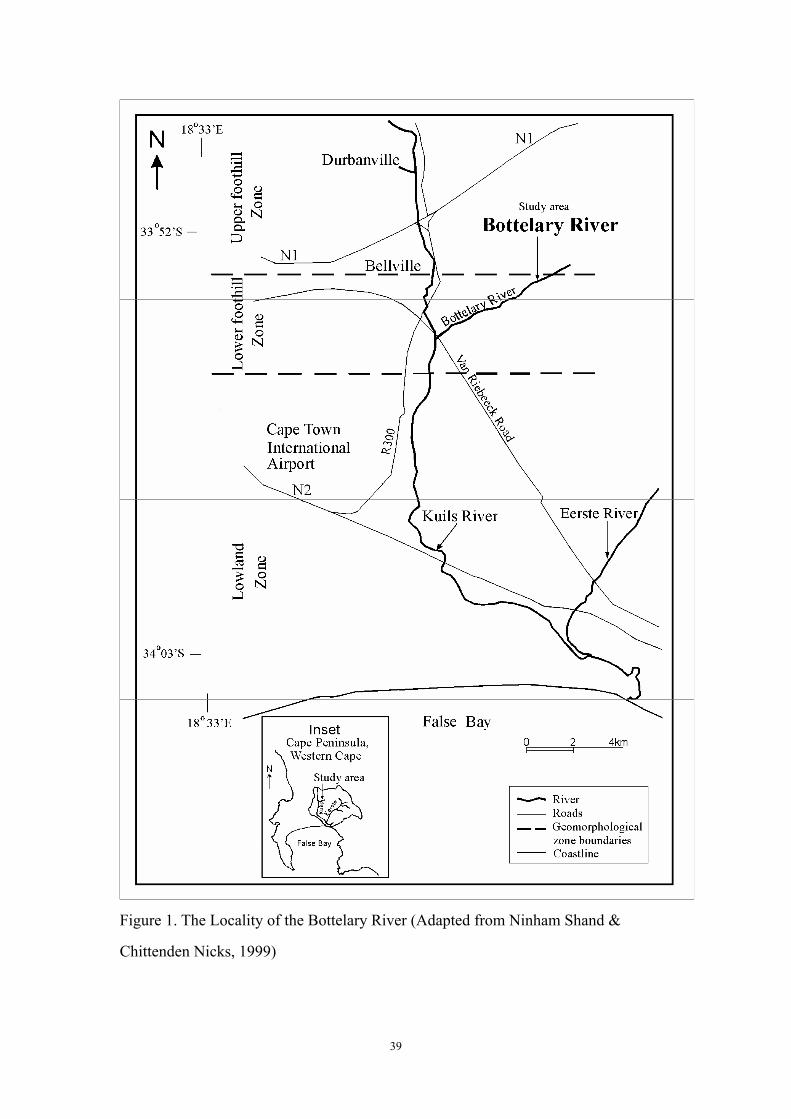
39

Figure 1. The Locality of the Bottelary River (Adapted from Ninham Shand &

Chittenden Nicks, 1999)

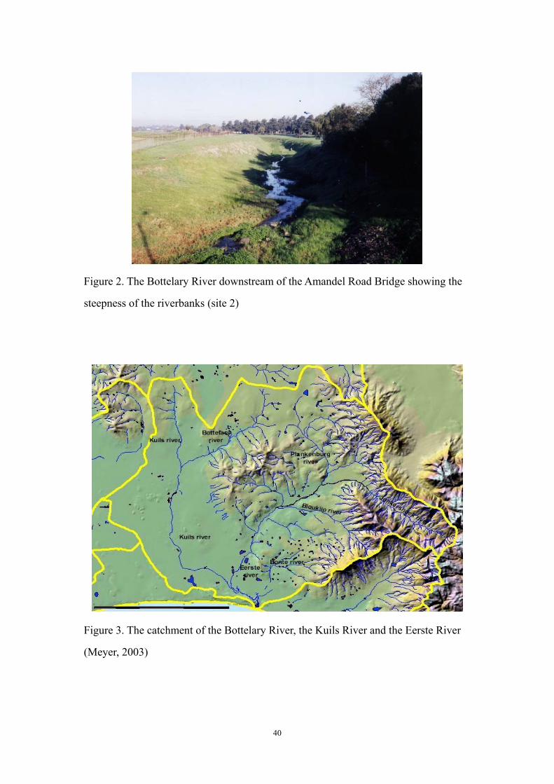
40

Figure 2. The Bottelary River downstream of the Amandel Road Bridge showing the

steepness of the riverbanks (site 2)

Figure 3. The catchment of the Bottelary River, the Kuils River and the Eerste River

(Meyer, 2003)

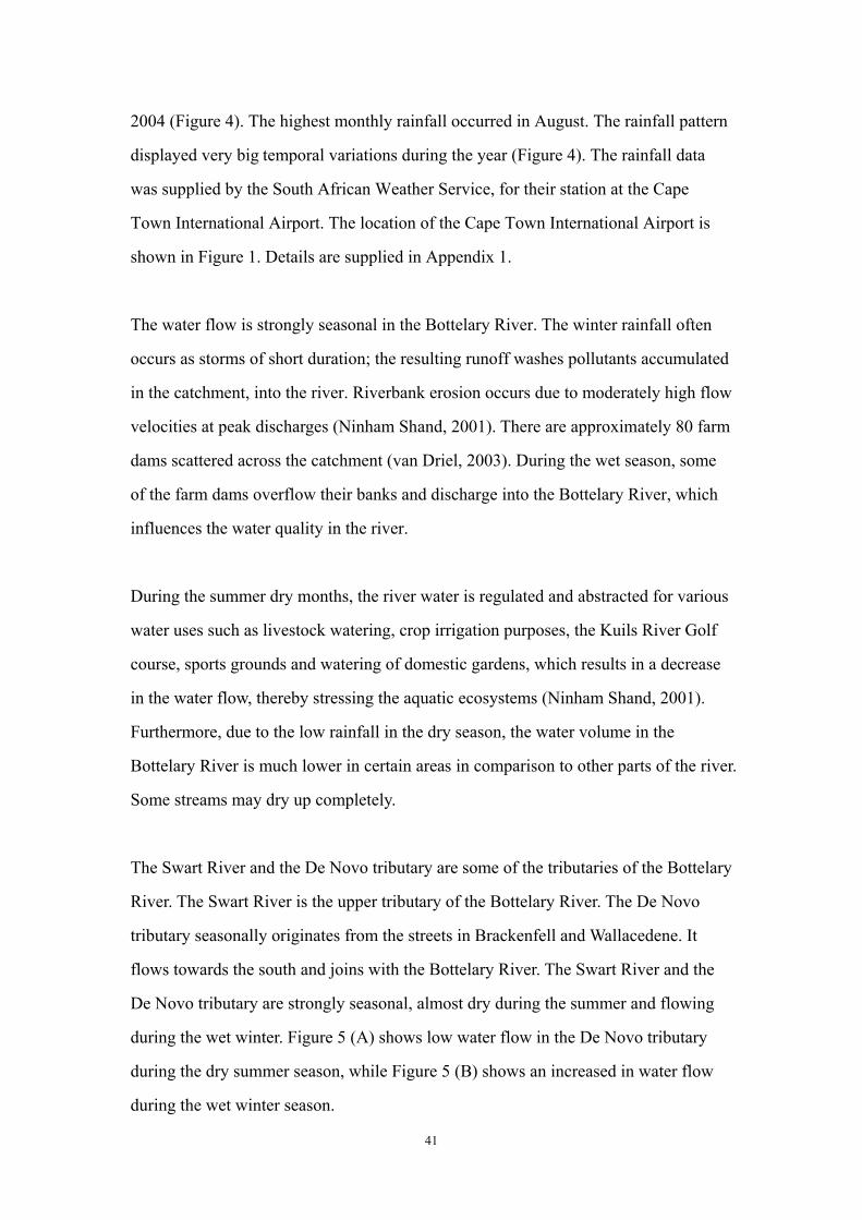
41

2004 (Figure 4). The highest monthly rainfall occurred in August. The rainfall pattern

displayed very big temporal variations during the year (Figure 4). The rainfall data

was supplied by the South African Weather Service, for their station at the Cape

Town International Airport. The location of the Cape Town International Airport is

shown in Figure 1. Details are supplied in Appendix 1.

The water flow is strongly seasonal in the Bottelary River. The winter rainfall often

occurs as storms of short duration; the resulting runoff washes pollutants accumulated

in the catchment, into the river. Riverbank erosion occurs due to moderately high flow

velocities at peak discharges (Ninham Shand, 2001). There are approximately 80 farm

dams scattered across the catchment (van Driel, 2003). During the wet season, some

of the farm dams overflow their banks and discharge into the Bottelary River, which

influences the water quality in the river.

During the summer dry months, the river water is regulated and abstracted for various

water uses such as livestock watering, crop irrigation purposes, the Kuils River Golf

course, sports grounds and watering of domestic gardens, which results in a decrease

in the water flow, thereby stressing the aquatic ecosystems (Ninham Shand, 2001).

Furthermore, due to the low rainfall in the dry season, the water volume in the

Bottelary River is much lower in certain areas in comparison to other parts of the river.

Some streams may dry up completely.

The Swart River and the De Novo tributary are some of the tributaries of the Bottelary

River. The Swart River is the upper tributary of the Bottelary River. The De Novo

tributary seasonally originates from the streets in Brackenfell and Wallacedene. It

flows towards the south and joins with the Bottelary River. The Swart River and the

De Novo tributary are strongly seasonal, almost dry during the summer and flowing

during the wet winter. Figure 5 (A) shows low water flow in the De Novo tributary

during the dry summer season, while Figure 5 (B) shows an increased in water flow

during the wet winter season.

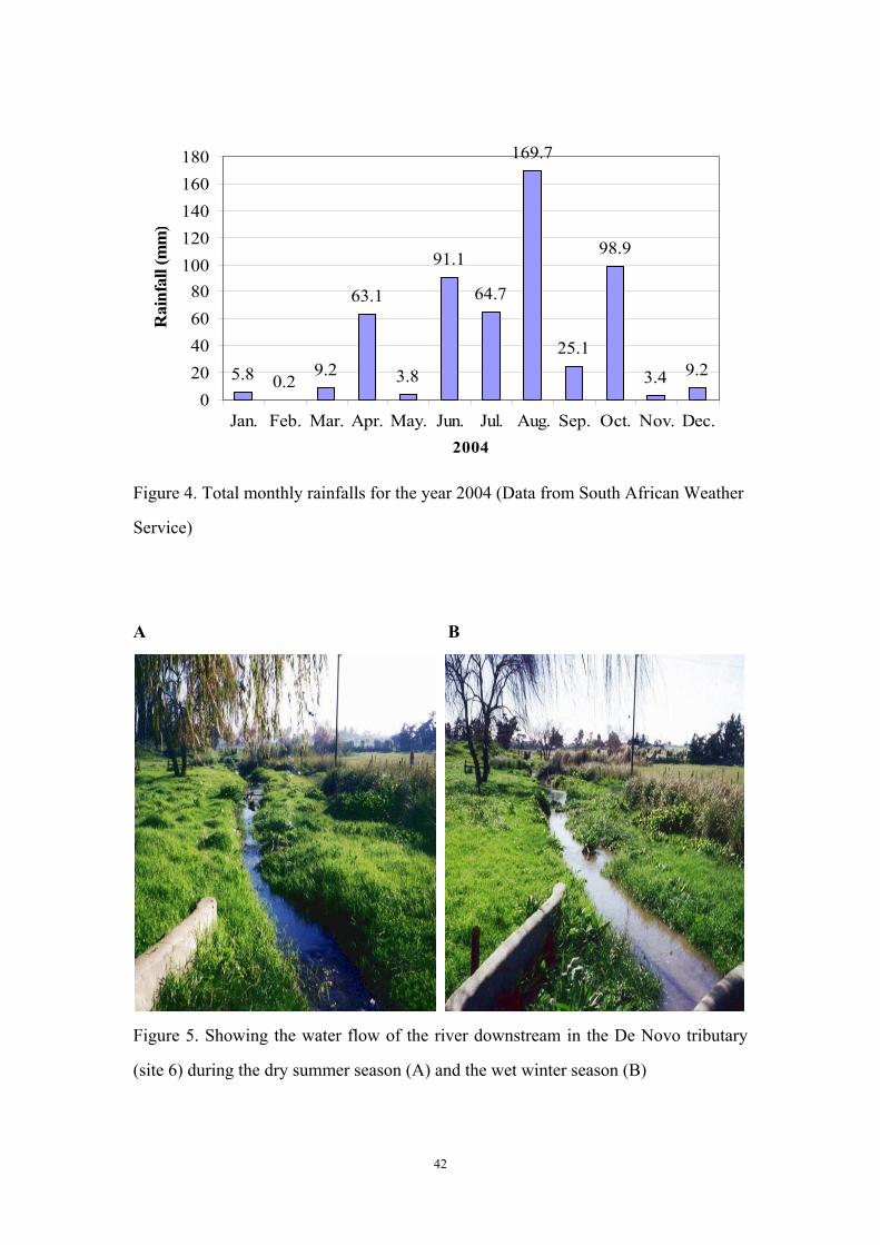
42

5.8 0.29.2

63.1

3.8

91.1

64.7

169.7

25.1

98.9

3.4 9.2

020406080

100120140160180

Jan. Feb. Mar. Apr. May. Jun. Jul. Aug. Sep. Oct. Nov. Dec.2004

Rai

nfal

l (m

m)

Figure 4. Total monthly rainfalls for the year 2004 (Data from South African Weather

Service)

A B

Figure 5. Showing the water flow of the river downstream in the De Novo tributary

(site 6) during the dry summer season (A) and the wet winter season (B)

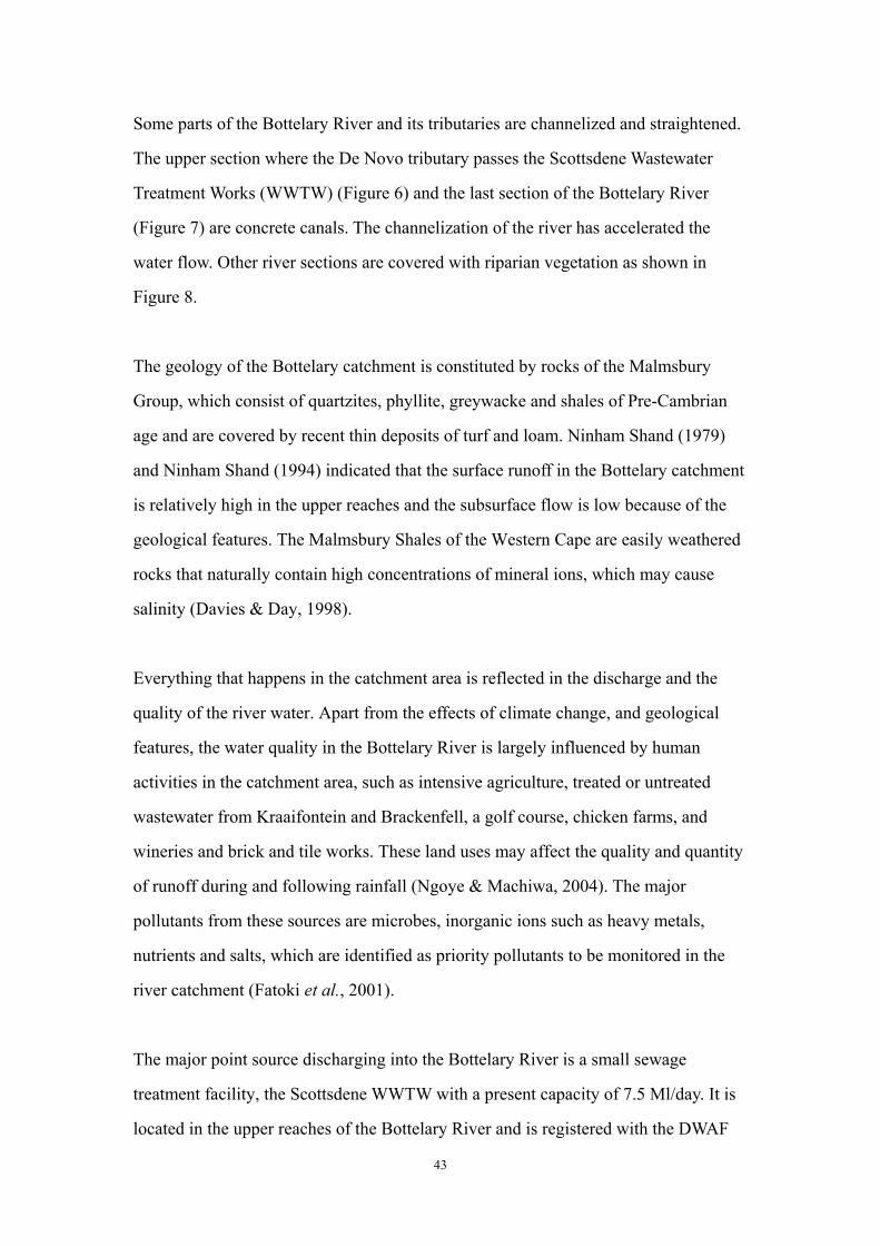
43

Some parts of the Bottelary River and its tributaries are channelized and straightened.

The upper section where the De Novo tributary passes the Scottsdene Wastewater

Treatment Works (WWTW) (Figure 6) and the last section of the Bottelary River

(Figure 7) are concrete canals. The channelization of the river has accelerated the

water flow. Other river sections are covered with riparian vegetation as shown in

Figure 8.

The geology of the Bottelary catchment is constituted by rocks of the Malmsbury

Group, which consist of quartzites, phyllite, greywacke and shales of Pre-Cambrian

age and are covered by recent thin deposits of turf and loam. Ninham Shand (1979)

and Ninham Shand (1994) indicated that the surface runoff in the Bottelary catchment

is relatively high in the upper reaches and the subsurface flow is low because of the

geological features. The Malmsbury Shales of the Western Cape are easily weathered

rocks that naturally contain high concentrations of mineral ions, which may cause

salinity (Davies & Day, 1998).

Everything that happens in the catchment area is reflected in the discharge and the

quality of the river water. Apart from the effects of climate change, and geological

features, the water quality in the Bottelary River is largely influenced by human

activities in the catchment area, such as intensive agriculture, treated or untreated

wastewater from Kraaifontein and Brackenfell, a golf course, chicken farms, and

wineries and brick and tile works. These land uses may affect the quality and quantity

of runoff during and following rainfall (Ngoye & Machiwa, 2004). The major

pollutants from these sources are microbes, inorganic ions such as heavy metals,

nutrients and salts, which are identified as priority pollutants to be monitored in the

river catchment (Fatoki et al., 2001).

The major point source discharging into the Bottelary River is a small sewage

treatment facility, the Scottsdene WWTW with a present capacity of 7.5 Ml/day. It is

located in the upper reaches of the Bottelary River and is registered with the DWAF

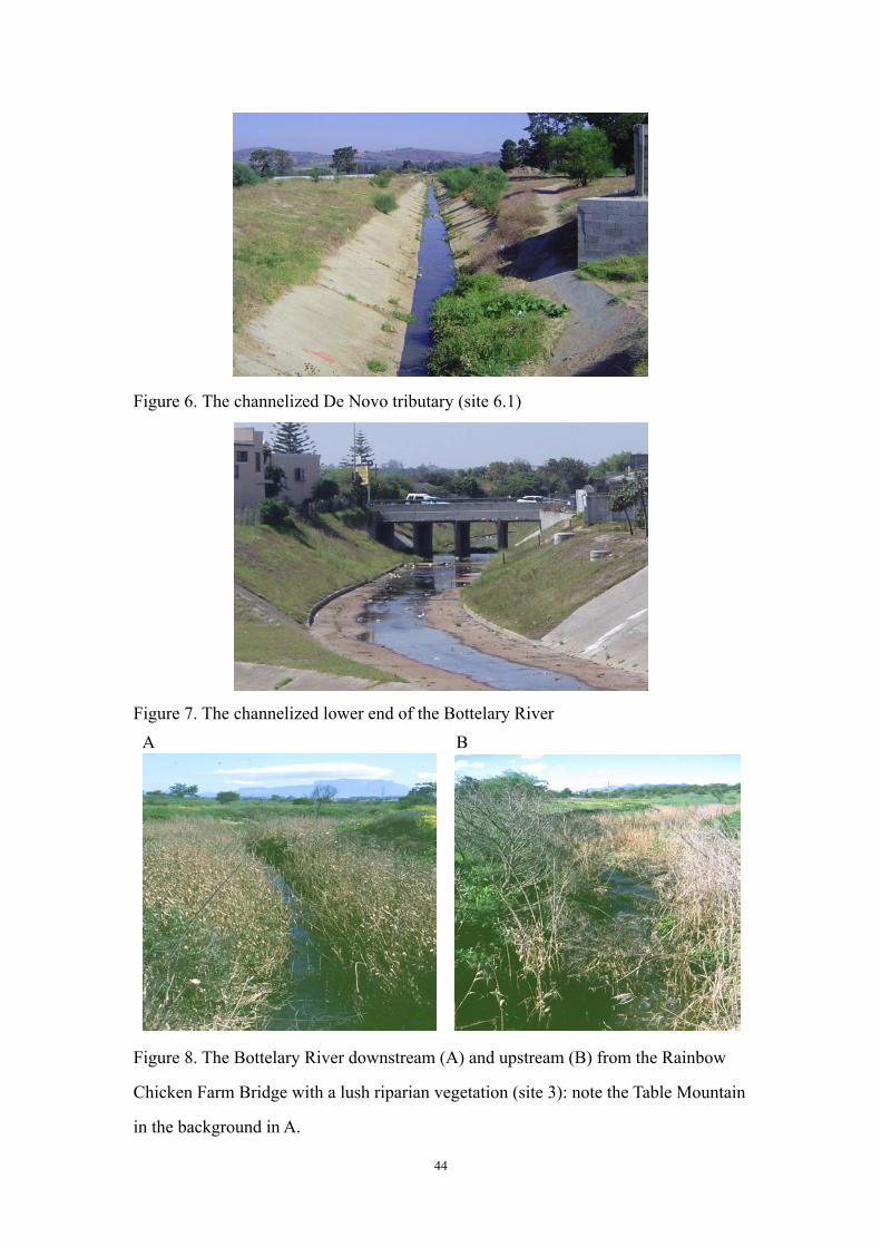
44

Figure 6. The channelized De Novo tributary (site 6.1)

Figure 7. The channelized lower end of the Bottelary River A B

Figure 8. The Bottelary River downstream (A) and upstream (B) from the Rainbow

Chicken Farm Bridge with a lush riparian vegetation (site 3): note the Table Mountain

in the background in A.

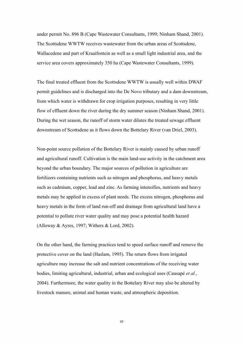
45

under permit No. 896 B (Cape Wastewater Consultants, 1999; Ninham Shand, 2001).

The Scottsdene WWTW receives wastewater from the urban areas of Scottsdene,

Wallacedene and part of Kraaifontein as well as a small light industrial area, and the

service area covers approximately 350 ha (Cape Wastewater Consultants, 1999).

The final treated effluent from the Scottsdene WWTW is usually well within DWAF

permit guidelines and is discharged into the De Novo tributary and a dam downstream,

from which water is withdrawn for crop irrigation purposes, resulting in very little

flow of effluent down the river during the dry summer season (Ninham Shand, 2001).

During the wet season, the runoff of storm water dilutes the treated sewage effluent

downstream of Scottsdene as it flows down the Bottelary River (van Driel, 2003).

Non-point source pollution of the Bottelary River is mainly caused by urban runoff

and agricultural runoff. Cultivation is the main land-use activity in the catchment area

beyond the urban boundary. The major sources of pollution in agriculture are

fertilizers containing nutrients such as nitrogen and phosphorus, and heavy metals

such as cadmium, copper, lead and zinc. As farming intensifies, nutrients and heavy

metals may be applied in excess of plant needs. The excess nitrogen, phosphorus and

heavy metals in the form of land run-off and drainage from agricultural land have a

potential to pollute river water quality and may pose a potential health hazard

(Alloway & Ayres, 1997; Withers & Lord, 2002).

On the other hand, the farming practices tend to speed surface runoff and remove the

protective cover on the land (Haslam, 1995). The return flows from irrigated

agriculture may increase the salt and nutrient concentrations of the receiving water

bodies, limiting agricultural, industrial, urban and ecological uses (Causapé et al.,

2004). Furthermore, the water quality in the Bottelary River may also be altered by

livestock manure, animal and human waste, and atmospheric deposition.

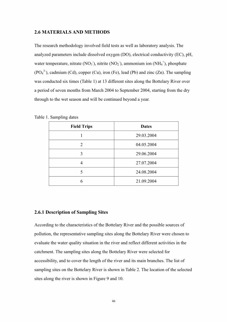
46

2.6 MATERIALS AND METHODS

The research methodology involved field tests as well as laboratory analysis. The

analyzed parameters include dissolved oxygen (DO), electrical conductivity (EC), pH,

water temperature, nitrate (NO3-), nitrite (NO2

-), ammonium ion (NH4+), phosphate

(PO43-), cadmium (Cd), copper (Cu), iron (Fe), lead (Pb) and zinc (Zn). The sampling

was conducted six times (Table 1) at 13 different sites along the Bottelary River over

a period of seven months from March 2004 to September 2004, starting from the dry

through to the wet season and will be continued beyond a year.

Table 1. Sampling dates

Field Trips Dates

1 29.03.2004

2 04.05.2004

3 29.06.2004

4 27.07.2004

5 24.08.2004

6 21.09.2004

2.6.1 Description of Sampling Sites

According to the characteristics of the Bottelary River and the possible sources of

pollution, the representative sampling sites along the Bottelary River were chosen to

evaluate the water quality situation in the river and reflect different activities in the

catchment. The sampling sites along the Bottelary River were selected for

accessibility, and to cover the length of the river and its main branches. The list of

sampling sites on the Bottelary River is shown in Table 2. The location of the selected

sites along the river is shown in Figure 9 and 10.

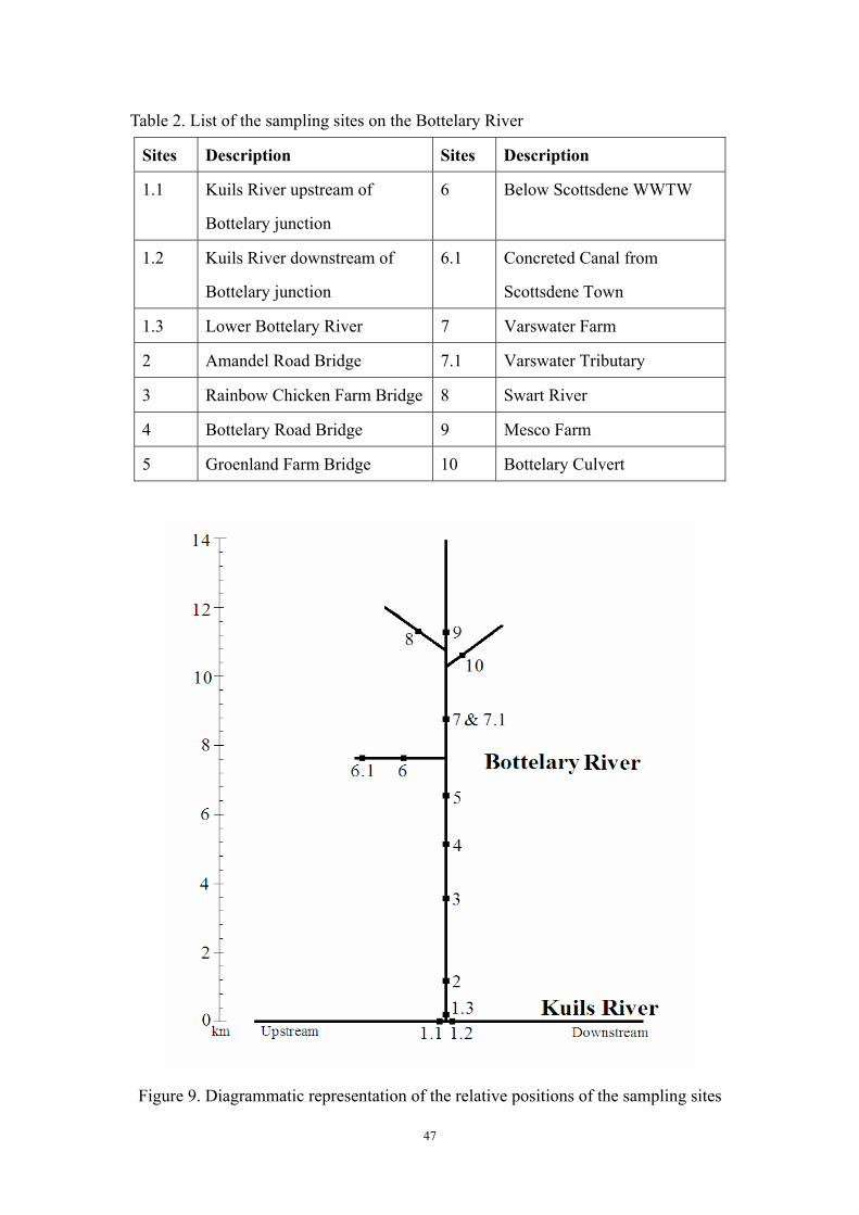
47

Table 2. List of the sampling sites on the Bottelary River

Sites Description Sites Description

1.1 Kuils River upstream of

Bottelary junction

6 Below Scottsdene WWTW

1.2 Kuils River downstream of

Bottelary junction

6.1 Concreted Canal from

Scottsdene Town

1.3 Lower Bottelary River 7 Varswater Farm

2 Amandel Road Bridge 7.1 Varswater Tributary

3 Rainbow Chicken Farm Bridge 8 Swart River

4 Bottelary Road Bridge 9 Mesco Farm

5 Groenland Farm Bridge 10 Bottelary Culvert

Figure 9. Diagrammatic representation of the relative positions of the sampling sites

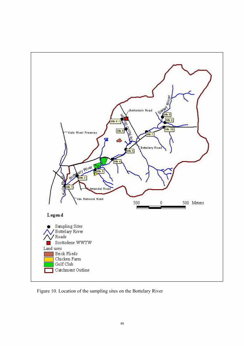
48

Figure 10. Location of the sampling sites on the Bottelary River

49

Three sampling sites were located around the junction of the Kuils River and the

Bottelary River to reflect the water quality in different systems as shown in Figure 11.

Site 1.1 was located just above the junction of the Kuils River and the Bottelary River

in the Kuils River. Site 1.2 was located in the Kuils River downstream of the

Bottelary River junction. Site 1.3 was located at the lower end of the Bottelary River.

Site 2 was located downstream of the Amandel Road Bridge (Figure 2). Site 3 (Figure

8) was a point located at a small bridge providing access to the Rainbow Chicken

Farm. Site 4 was located at the Bottelary Road Bridge that crosses the middle of the

river. Site 5 was located at a bridge on the Groenland Farm as shown in Figure 12.

Site 6 (Figure 5) was located below the Scottsdene WWTW in the De Novo tributary

so that the impact of effluent discharge from Scottsdene WWTW on the water quality

in the river could be assessed. Measurement point 6.1 was located upstream in the

concreted De Novo tributary, running from Scottsdene in Kraaifontein as shown in

Figure 6, which was chosen in order to investigate urban runoff from Scottsdene.

Site 7 was located at a small bridge on the Varswater Farm (Figure 13); site 7.1 was a

small additional tributary which ran during August and September. Site 8 was situated

in the upper tributary, the Swart River (Figure 14). Site 9 was located on the Mesco

Farm as shown in Figure 15. Site 10 was at the Bottelary culvert where the Bottelary

Road crosses the upper river. Site 11 was situated in a dam that collects the winery

effluent upstream of site 9.

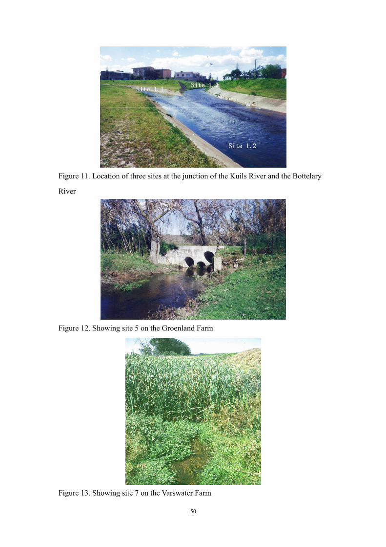
50

Figure 11. Location of three sites at the junction of the Kuils River and the Bottelary

River

Figure 12. Showing site 5 on the Groenland Farm

Figure 13. Showing site 7 on the Varswater Farm

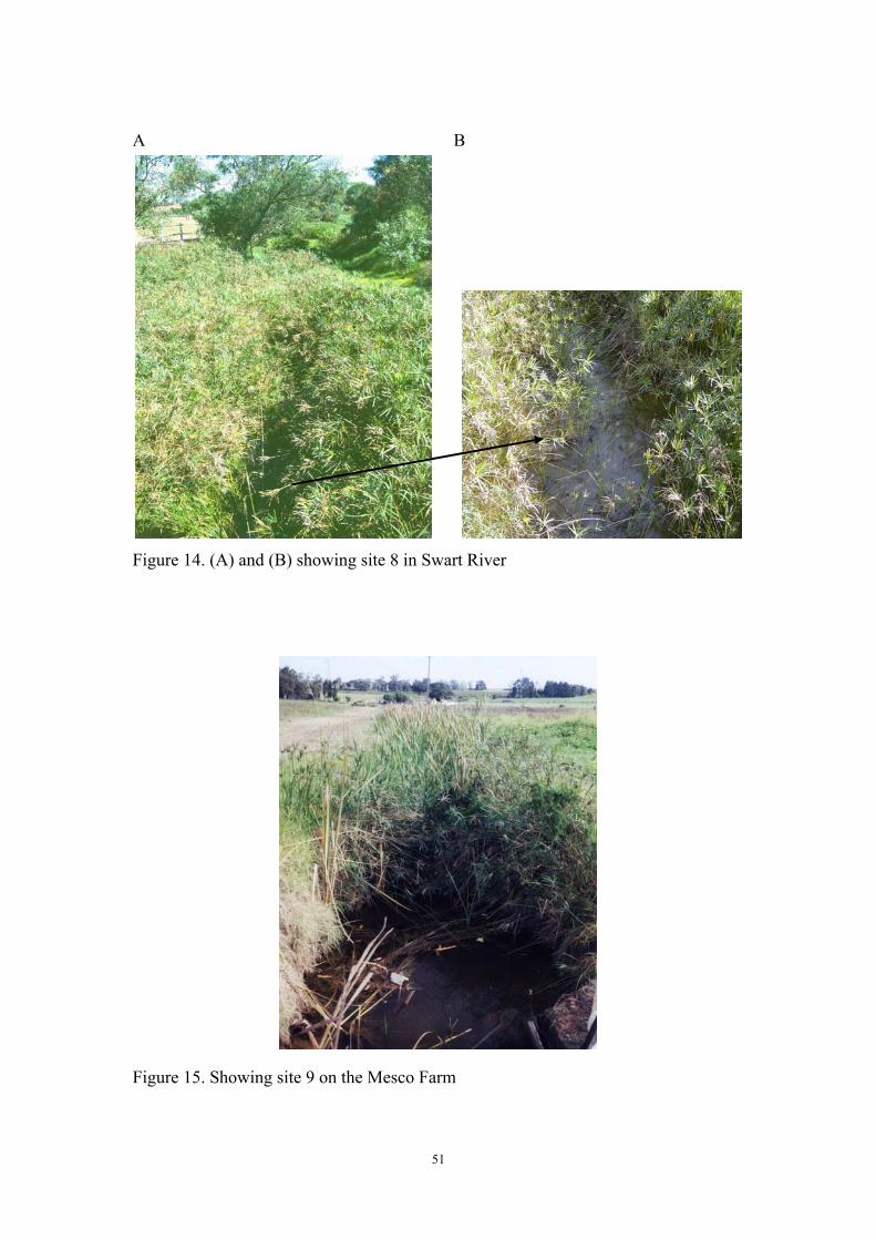
51

A B

Figure 14. (A) and (B) showing site 8 in Swart River

Figure 15. Showing site 9 on the Mesco Farm

52

2.6.2 Field Procedures

Water samples were collected six times, using clean 500 ml plastic sampling bottles,

at different sampling sites. Dissolved oxygen and water temperature were determined

in the field for each site using a handheld dissolved oxygen meter (YSI Model 55

Handheld Dissolved Oxygen System, Japan). Dissolved oxygen was reported as

milligrams per liter (mg/l), while water temperature was reported as degree centigrade

(ºC).

2.6.3 Laboratory Procedures

Water samples were analyzed as soon as possible in the laboratory for pH, electrical

conductivity, nitrate, nitrite and ammonia. They were then filtered, acidified, and

stored at 4 ºC until all the sample collections had been made. Finally, the phosphate

and the heavy metals concentrations were determined.

The water samples were measured for hydrogen ion activity using a pH meter (PHM

64 Research pH meter, Radiometer Copenhagen) and for electrical conductivity using

a conductivity meter (Metrohm 644 conductometer, Switzerland) as a measure of

salinity. A 0.5 cm-3 aliquot of hydrochloric acid (HCL) was added per 100 cm-3 of

water before storage in a cold room.

2.6.4 Nitrogen Analysis

For nitrogen, three components were measured: nitrate, nitrite and ammonium ion.

The concentration of inorganic nitrogen species in water is obtained by adding

together the individual concentrations of nitrate, nitrite and ammonia (DWAF, 1996 d).

Aquamerck Reagent Kits were used to estimate levels of nitrate, nitrite and

ammonium ion in the laboratory. The detection limits for nitrogen by Aquamerck

Reagent Kits were 2.5 mg/l for nitrate, 0.013 mg/l for nitrite and 0.25 mg/l for

53

ammonium ion.

Nitrate was measured by using a Merck Nitrate Kit (AquamerckR 8032 Nitrate

MERCK), which uses the reduction of nitrate to nitrite through the formation of an

azo dye with sulphanilic/gentisic acid. The reagent kit included a colour scale.

Comparison with the colour scale permits a rapid and semiquantitative assessment of

the nitrate content present.

Nitrite was estimated using a Merck Nitrite Kit (AquamerckR 8025 Nitrite MERCK)

which uses colorimetric determination with sulfanilic acid and N-(1-naphty1)

ethylenediammonium dichloride reagent, with a colour scale. In acidic solution, nitrite

ions react with sulfanilic acid to form a coloured diazonium salt and then reacts with

N-(1-naphty1) ethylenediammonium dichloride to form a red-violet azo dye. The

colour formation was used to estimate the nitrite concentration by visual comparison

of the colours of the solution with the colour standards.

Ammonium was determined in the laboratory using a Merck Ammonium Kit

(AquamerckR 11 117 Ammonium Test MERCK), which uses colorimetric

determination with Nessler’s reagent with a colour scale. Ammonium ions react with

Nessler’s reagent to form a characteristic yellow to brown dye. Again, a colour scale

enabled estimations of ammonium levels.

2.6.5 Phosphorus Analysis

Phosphorus in natural waters is usually found in the form of phosphates and its

concentrations are usually determined as orthophosphates, total inorganic phosphate or

total dissolved phosphorus (which includes organically bound phosphorus and all

phosphates). The operational categories of phosphates are soluble reactive phosphate,

soluble unreactive phosphate, particulate reactive phosphate, and particulate unreactive

54

phosphate. The most commonly measured is Soluble Reactive Phosphate (SRP), which

is referred to as orthophosphate (DWAF, 1996 b).

The phosphate in the water samples was determined by using the ascorbic

acid-molybdate blue method of Murphy and Riley (1962), which is based on the

finding that antimony (as potassium antimonyl tartrate solution) reacts with phosphate

solution containing the original single solution reagent (Murphy and Riley solution) to

form an intense bluish-purple colour. The Murphy and Riley solution was made from

a mixture of four reagents: sulphuric acid, ammonium molybdate, ascorbic acid, and

potassium antimonyl tartrate (Murphy & Riley, 1962).

During the Murphy and Riley procedure, a standard phosphate solution was made in

order to produce a standard curve before running the digested samples. The colour

was allowed to develop for one hour and the absorbance was measured at 882 nm.

One ml of unknown sample was pipetted into a fifty ml volumetric flask, and

twenty-five ml of distilled water were added. Eight ml of the Murphy and Riley

solution were then added and made up to volume with distilled water and thoroughly

mixed. The resultant solutions were measured for their absorbance by using a

Shimadzu 160-A UV visible recording spectrophotometer. The detection limit of

phosphate by Murphy and Riley (1962) method was in the order of 0.1µg/l.

The phosphate was calculated using the following formula:

P (mg/l) (water) = Concentration (mg) ×1000/aliquot (ml) (Allen et al., 1986)

2.6.6 Heavy Metals Analysis

The water samples were analyzed to determine the concentrations of cadmium, copper,

and lead by using a Unicam Solaar M Series Atomic Absorption Spectrometer (AAS)

with GF95 Graphite Furnace System. The detection limits were 0.56 pg/l for cadmium,

1.8 pg/l for copper and 1.5 pg/l for lead. The concentrations of iron and zinc were

55

determined by using the same instrument with an air/acetylene flame system. The

detection limits were 0.06 pg/l for iron and 0.013 pg/l for zinc.

2.6.7 Statistical Analysis

The statistical analysis was based on the raw data in the Appendix 2. This analysis

was professionally carried out by the Agricultural Research Council using SAS

Version 8.2 (SAS, 1999).

2.6.8 Comparison of Results with the South African Water Quality

Guidelines

The South African Water Quality Guideline series was published by the Department

of Water Affairs and Forestry for water resource protection and water quality

management. In order to compare the results to the South African Water Quality

Guidelines the background concentrations of the particular water sources need to be

known. To estimate the background concentration of a water quality constituent there

has to be a data set covering at least one hydrological cycle for an unimpacted point at

which:

• there are no identifiable point or diffuse sources upstream; and

• there are enough data available to be certain that there is no temporal trend at the

85% confidence interval.

The background concentration is then taken to be the 90-percentile concentration of the

water quality constituent in this data set (DWAF, 1996 d). For the portion of the

Bottelary River that was studied, it was not possible to determine the background

concentration of the water quality parameters as there was neither enough data covering

a single hydrological cycle nor was there any portion that could be considered as not

being impacted by various sources.

56

The water hardness is defined as the sum of the calcium ions (Ca2+) and magnesium

ion (Mg2+) concentrations, both expressed as carbonate, in milligrams per liter

(DWAF, 1996 d; Baird & Cann, 2005). The South African Water Quality Guidelines

define the water as being medium if its hardness index lies between 60–119 mg/l and

as being soft if its hardness index is below 60 mg/l (DWAF, 1996 d). According to the

historical results obtained by van Driel (2003), the sum of the Ca2+ and Mg2+

concentrations in the Bottelary River was 95.6 mg/l in July 2003 (winter) and was

48.5–50.7 mg/l in January and February 2001 (summer), which was within the

medium and soft ranges.

57

2.7 RESULTS AND DISCUSSION

The raw data are available in Appendix 2.

2.7.1 Nitrogen Concentrations

The (inorganic) nitrogen in water usually occurs in the form of nitrate, nitrite and

ammonium ion (Davies & Day, 1998). Nitrate is the end product of the oxidation of

nitrite or ammonia and does not cause direct toxic effects (DWAF, 1996 c&d). Nitrite

is the inorganic intermediate of the inter-conversion of nitrate and ammonia (Davies

& Day, 1998). It causes direct toxic effects to aquatic organisms and is 10–15 times

more toxic than nitrate (DWAF, 1996 c). In the aquatic environment, the

inter-conversion between nitrates and nitrites readily occurs. Under oxidizing

conditions nitrite is converted to nitrate, which is usually far more abundant in the

aquatic environment than nitrite (DWAF, 1996 c&d).

Ammonia is reduced form of inorganic nitrogen and can occur either in a free

un-ionized form (NH3) or in an ionized form as ammonium ion (NH4+) (DWAF, 1996

d). In solution, un-ionized ammonia occurs in equilibrium with the ammonium ion

(DWAF, 1996 a). The relative proportion and toxicity of un-ionized ammonia are

significantly affected by pH and water temperature (DWAF, 1996 d). The ammonia

toxicity is also influenced by the concentrations of dissolved oxygen, carbon dioxide

and total dissolved solids, and the presence of other toxicants, such as metal ions. The

ammonium ion generally has little or no toxicity to aquatic biota, but contributes to

eutrophication (DWAF, 1996 d).

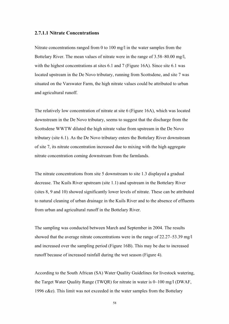
58

2.7.1.1 Nitrate Concentrations

Nitrate concentrations ranged from 0 to 100 mg/l in the water samples from the

Bottelary River. The mean values of nitrate were in the range of 3.58–80.00 mg/l,

with the highest concentrations at sites 6.1 and 7 (Figure 16A). Since site 6.1 was

located upstream in the De Novo tributary, running from Scottsdene, and site 7 was

situated on the Varswater Farm, the high nitrate values could be attributed to urban

and agricultural runoff.

The relatively low concentration of nitrate at site 6 (Figure 16A), which was located

downstream in the De Novo tributary, seems to suggest that the discharge from the

Scottsdene WWTW diluted the high nitrate value from upstream in the De Novo

tributary (site 6.1). As the De Novo tributary enters the Bottelary River downstream

of site 7, its nitrate concentration increased due to mixing with the high aggregate

nitrate concentration coming downstream from the farmlands.

The nitrate concentrations from site 5 downstream to site 1.3 displayed a gradual

decrease. The Kuils River upstream (site 1.1) and upstream in the Bottelary River

(sites 8, 9 and 10) showed significantly lower levels of nitrate. These can be attributed

to natural cleaning of urban drainage in the Kuils River and to the absence of effluents

from urban and agricultural runoff in the Bottelary River.

The sampling was conducted between March and September in 2004. The results

showed that the average nitrate concentrations were in the range of 22.27–53.39 mg/l

and increased over the sampling period (Figure 16B). This may be due to increased

runoff because of increased rainfall during the wet season (Figure 4).

According to the South African (SA) Water Quality Guidelines for livestock watering,

the Target Water Quality Range (TWQR) for nitrate in water is 0–100 mg/l (DWAF,

1996 c&e). This limit was not exceeded in the water samples from the Bottelary

59

A

aababcabcabc

bcdcdcd

e

de

e e e0

102030405060708090

100

1.1 1.2 1.3 2 3 4 5 6 6.1 7 8 9 10Sampling sites

NO

3- (mg/

l)

B

cbc

abab

a a

0

10

20

30

40

50

60

0 50 100 150 200 250 300Time (days)

NO

3- (mg/

l)

Figure 16. Means with the same letter are not significantly different at p=0.05.

(A) Nitrate levels (mg/l) at the sampling sites on the Bottelary River over the

sampling period (2004). (B) Seasonal variation of nitrate in the Bottelary River and its

main tributaries.

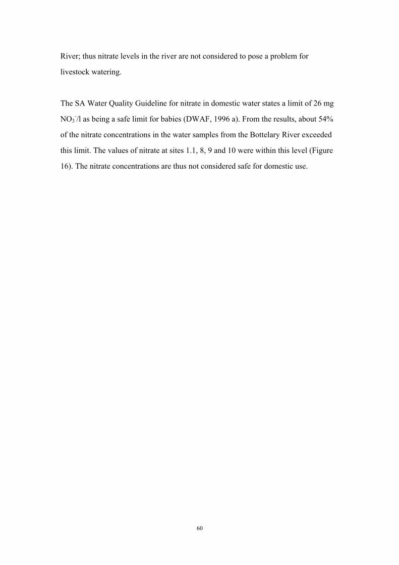
60

River; thus nitrate levels in the river are not considered to pose a problem for

livestock watering.

The SA Water Quality Guideline for nitrate in domestic water states a limit of 26 mg

NO3-/l as being a safe limit for babies (DWAF, 1996 a). From the results, about 54%

of the nitrate concentrations in the water samples from the Bottelary River exceeded

this limit. The values of nitrate at sites 1.1, 8, 9 and 10 were within this level (Figure

16). The nitrate concentrations are thus not considered safe for domestic use.

61

2.7.1.2 Nitrite Concentrations

Nitrite concentrations ranged between 0 and 2 mg/l. The mean values of nitrite were

in the range of 0.019–1.150 mg/l. The highest mean value of nitrite was noted at site

6.1 (concreted canal from Scottsdene) upstream in the De Novo tributary (Figure 17

A). This high nitrite value could be attributed to urban runoff from Scottsdene. The

nitrite concentrations gradually decreased away from this polluted source (site 6.1),

towards the junction of the Kuils River and the Bottelary River.

The concentrations of nitrite were significantly lower at sites 7, 8, 9 and 10 in the

upper section of the Bottelary River and at site 1.1 in the Kuils River (Figure 17A),

which showed that the impact of nitrite in these river sections was lower.

During the study period, the mean concentrations of nitrite were in the range of

0.07–0.54 mg/l and increased (Figure 17B), probably due to increased runoff because

of increased rainfall during the wet season (Figure 4).

The SA Water Quality Guideline for nitrite in water to be used for livestock watering

is 0–10 mg/l (DWAF, 1996 e). This level was not exceeded in the water samples from

the Bottelary River. Thus, the water use from the river for livestock should not cause

nitrite poisoning.

The SA Water Quality Guideline for nitrite in domestic water is 20 mg NO2-/l as a

safe limit for babies (DWAF, 1996 a). This limit was not exceeded in the water

samples. However, the World Health Organization (WHO) safe limit guideline for

short-term exposure is 3 mg/l and for long-term exposure is 0.2 mg/l (WHO, 2004).

The nitrite values in the water samples did not exceed the limit for short-term

exposure, but exceeded the limit for long-term exposure. The nitrite concentrations

are thus considered to pose a problem for domestic use.

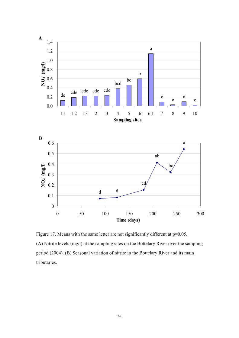
62

A

a

bbc

bcdcdecde cde

de cdeee e e

0.0

0.2

0.4

0.6

0.8

1.0

1.2

1.4

1.1 1.2 1.3 2 3 4 5 6 6.1 7 8 9 10Sampling sites

NO

2- (mg/

l)

B

d dcd

bc

ab

a

0

0.1

0.2

0.3

0.4

0.5

0.6

0 50 100 150 200 250 300Time (days)

NO

2- (mg/

l)

Figure 17. Means with the same letter are not significantly different at p=0.05.

(A) Nitrite levels (mg/l) at the sampling sites on the Bottelary River over the sampling

period (2004). (B) Seasonal variation of nitrite in the Bottelary River and its main

tributaries.

63

2.7.1.3 Ammonia Concentrations

The ammonium ion concentrations ranged from 0 to 10 mg/l. The mean values of

ammonium ion varied between 0.33 and 6.17 mg/l. Figure 18 (A) shows that the mean

concentrations of ammonium ion were significantly higher at site 6 (below the

Scottsdene WWTW) and site 6.1(concreted canal from Scottsdene) in the De Novo

tributary. The distinct peak in the concentrations of ammonium ion could have

resulted from the discharge of treated sewage effluent from the Scottsdene WWTW

and urban runoff from Scottsdene. The values of ammonium ion were significantly

lower in the Kuils River and the main course of the Bottelary River, which were less

impacted.

Figure 18 (B) shows that average ammonium ion concentrations were in the range of

0.69–2.40 mg/l and increased over the study period probably due to increased runoff

because of increased rainfall during wet season (Figure 4).

The SA Target Water Quality Range for ammonia in aquatic ecosystems is based on

the un-ionised ammonia fraction, which is 0–0.007 mg NH3/l (DWAF, 1996d). The

Chronic Effect Value (CEV) is 0.015 mg NH3/l and the Acute Effect Value (AEV) is

0.1 mg NH3/l. The guideline states that ammonium ions are converted to the highly

toxic un-ionized ammonia when the pH value is above eight. Ammonia is found

predominantly as ammonium ion in water at low and near-neutral pH, while at high pH

(approximately 11), un-ionized ammonia predominates as a gas in solution, the latter

being considerably more toxic to aquatic organisms, but it can be released to the

atmosphere from the water. The percentage ammonia also increased with increased

water temperature (DWAF, 1996 d).

The average ammonia concentrations for the sites in the De Novo tributary, estimated

from the table provided by DWAF (1996 d) for 20˚C and pH 7.5, are approximately ten

times the Target Water Quality Range maximum. This is well above the Chronic Effect

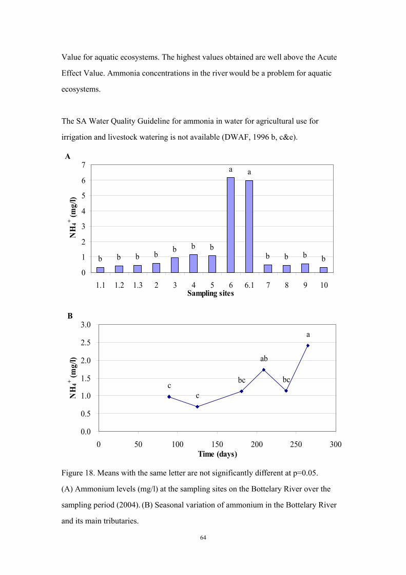
64

Value for aquatic ecosystems. The highest values obtained are well above the Acute

Effect Value. Ammonia concentrations in the river would be a problem for aquatic

ecosystems.

The SA Water Quality Guideline for ammonia in water for agricultural use for

irrigation and livestock watering is not available (DWAF, 1996 b, c&e).

A

bbbb b b bb b bb

aa

0

1

2

3

4

5

6

7

1.1 1.2 1.3 2 3 4 5 6 6.1 7 8 9 10Sampling sites

NH

4+ (mg/

l)

B

a

ab

bcbc

cc

0.0

0.5

1.0

1.5

2.0

2.5

3.0

0 50 100 150 200 250 300Time (days)

NH

4+ (mg/

l)

Figure 18. Means with the same letter are not significantly different at p=0.05.

(A) Ammonium levels (mg/l) at the sampling sites on the Bottelary River over the

sampling period (2004). (B) Seasonal variation of ammonium in the Bottelary River

and its main tributaries.

65

2.7.1.4 Total Nitrogen Concentrations

Total nitrogen concentrations in the water samples from the Bottelary River were in

the range of 0.21–102.60 mg/l. The mean values of total nitrogen ranged from 3.94 to

87.15 mg/l. Figure 19 (A) shows that the maximum mean concentrations of total

nitrogen were observed at site 6.1 (concreted canal from Scottsdene) and site 7

(Varswater Farm). The minimum mean concentrations were found in the Kuils River

upstream of the Bottelary River junction (site 1.1) and upstream in the Bottelary River

(sites 8, 9 and 10).

Figure 19 (B) shows that the mean concentrations of total nitrogen varied between

23.32 and 56.33 mg/l, and increased over the study period probably due to increased

runoff because of increased rainfall during wet season (Figure 4).

The spatial and temporal distributions pattern of total nitrogen is similar to that of

nitrate (see discussion on nitrate under section 2.7.1.1) because nitrate is the major

component of total nitrogen. The results indicated that the total nitrogen in the

Bottelary River mainly came from urban runoff from Scottsdene and agricultural

runoff from the Varswater Farm. There was relatively less impact of nitrogen in the

Kuils River above the Bottelary junction and upstream in the Bottelary River.

According to the SA Water Quality Guidelines for aquatic ecosystems (DWAF, 1996

d), the nitrogen criterion (Table 3) is based on summer values due to the enhanced

effects on plant growth at higher temperature. The dry season values, though the

lowest we obtained (Figure 19B), were in the hypertrophic range (Table 3). The high

values of nitrogen would be a problem in the Bottelary River because of

eutrophication.

The SA Target Water Quality Range for nitrogen in water to be used in agricultural

irrigation equipment is 0–0.5 mg/l, while that for crop yield, quality, and prevention

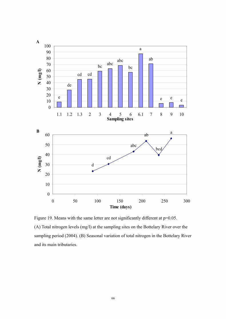
66

A

eee

de

e

cd cdbcbc abc

abc ab

a

0102030405060708090

100

1.1 1.2 1.3 2 3 4 5 6 6.1 7 8 9 10Sampling sites

N (m

g/l)

B aab

bcdabc

cdd

0

10

20

30

40

50

60

0 50 100 150 200 250 300Time (days)

N (m

g/l)

Figure 19. Means with the same letter are not significantly different at p=0.05.

(A) Total nitrogen levels (mg/l) at the sampling sites on the Bottelary River over the

sampling period (2004). (B) Seasonal variation of total nitrogen in the Bottelary River

and its main tributaries.

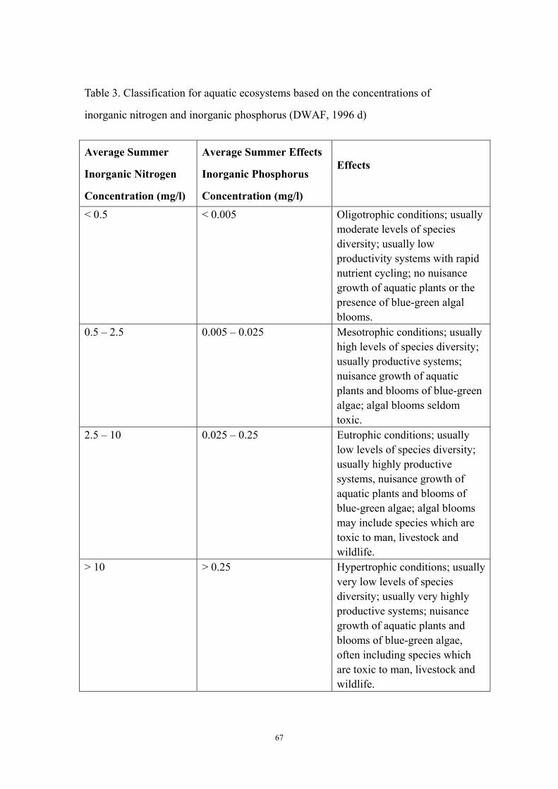
67

Table 3. Classification for aquatic ecosystems based on the concentrations of

inorganic nitrogen and inorganic phosphorus (DWAF, 1996 d)

Average Summer

Inorganic Nitrogen

Concentration (mg/l)

Average Summer Effects

Inorganic Phosphorus

Concentration (mg/l)

Effects

< 0.5 < 0.005 Oligotrophic conditions; usually moderate levels of species diversity; usually low productivity systems with rapid nutrient cycling; no nuisance growth of aquatic plants or the presence of blue-green algal blooms.

0.5 – 2.5 0.005 – 0.025 Mesotrophic conditions; usually high levels of species diversity; usually productive systems; nuisance growth of aquatic plants and blooms of blue-green algae; algal blooms seldom toxic.

2.5 – 10 0.025 – 0.25 Eutrophic conditions; usually low levels of species diversity; usually highly productive systems, nuisance growth of aquatic plants and blooms of blue-green algae; algal blooms may include species which are toxic to man, livestock and wildlife.

> 10 > 0.25 Hypertrophic conditions; usually very low levels of species diversity; usually very highly productive systems; nuisance growth of aquatic plants and blooms of blue-green algae, often including species which are toxic to man, livestock and wildlife.

68

of groundwater contamination is 0–5 mg/l (DWAF, 1996 b&e). The values of total

nitrogen in the water samples from the Bottelary River significantly exceeded these

limits, which indicated that the high concentrations of nitrogen would be a problem if

the water to be used directly for agricultural irrigation.

The high values of nitrogen in the irrigation water could cause adverse effects on

crops (by its stimulatory effect on the growth of weeds leading to delayed crop

maturity and poor crop quality), increased likelihood of leaching and contaminating

groundwater, and continuous growth of nuisance plants and blue-green algal blooms

in irrigation structures in the absence of other growth-limiting factors (DWAF, 1996

b).

The SA Water Quality Guideline for nitrogen in water to be used for livestock

watering is not available (DWAF, 1996 c&e).

69

2.7.2 Phosphorous Concentrations

Phosphorus is an essential macronutrient in life processes and is considered to be the

principle nutrient controlling the degree of eutrophication in aquatic ecosystems

(DWAF, 1996 d). The addition of large quantities of phosphorus accelerates algal and

macrophyte growth in natural waters, enhancing eutrophication.

The phosphate concentrations in the water samples from the Bottelary River were in

the range of 0–25.809 mg/l. The mean values of phosphate ranged from 0.527 to

18.202 mg/l. The highest mean concentration of phosphate was noted at site 6, below

the effluent discharge point from the Scottsdene WWTW in the De Novo tributary

(Figure 20A). Thus the high levels of phosphate in the Bottelary River could be

attributed to the effluent discharge from the Scottsdene WWTW.

The phosphate concentrations displayed a gradual decrease from site 6 to the lower

Bottelary River (site 1.3). There were significantly lower phosphate values in the

Kuils River above the Bottelary junction (site 1.1) and upstream in the Bottelary River

(sites 8, 9 and 10) (Figure 20A), which may be due to the absence of effects of the

effluent discharge from the Scottsdene WWTW on these river sections. The mean

phosphate value at site 1.2 differed from most other sites due to the dilution from the

Kuils River.

During the period of investigation, the mean concentrations of phosphate were

generally in the range of 4.52–9.79 mg/l and increased (Figure 20B). It may be due to

increased runoff because of increased rainfall during wet season (Figure 4). Data from

the Scottsdene WWTW also suggests an increase in phosphate concentrations in the

effluent over the study period as shown in Figure 21 (Scientific Services, City of Cape

Town, 2004).

According to the SA Water Quality Guidelines for aquatic ecosystems, the phosphorus

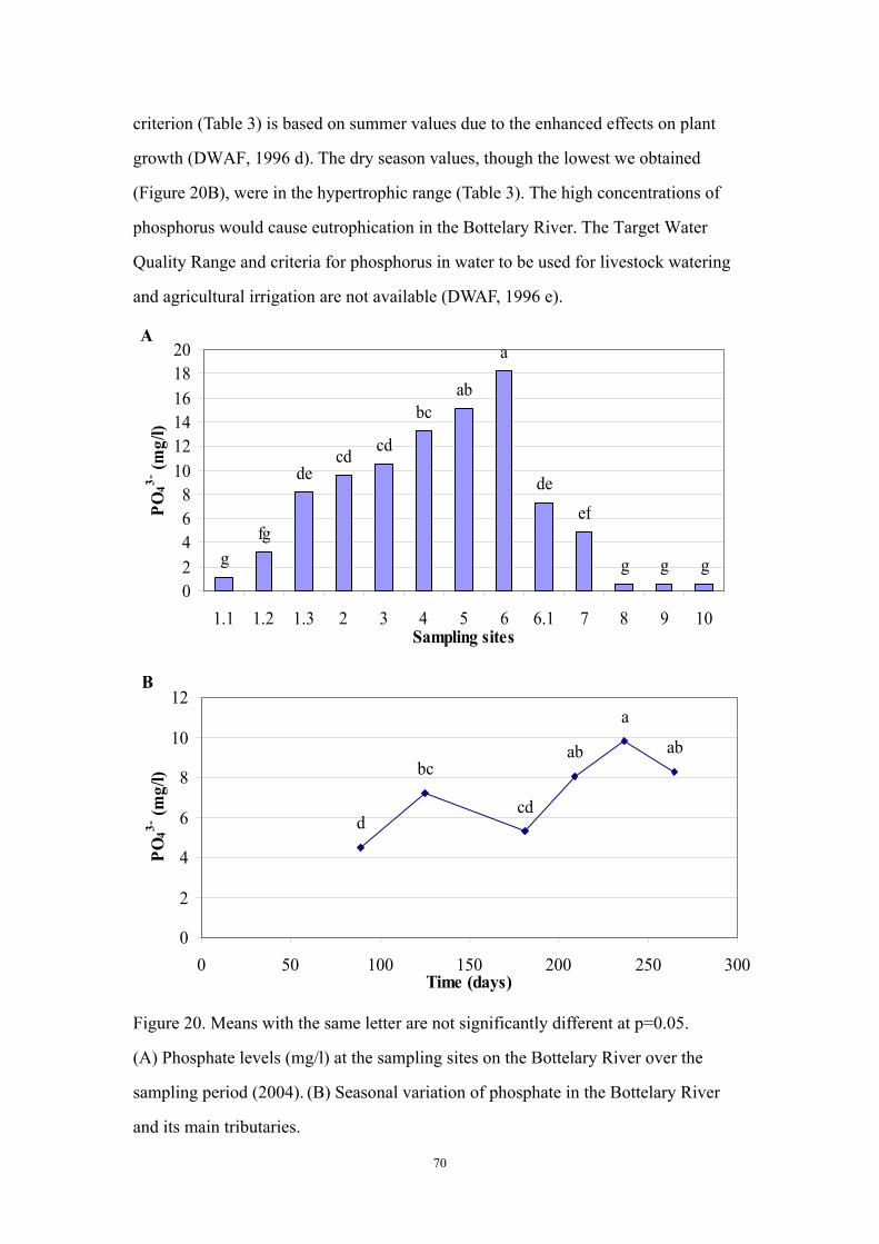
70

criterion (Table 3) is based on summer values due to the enhanced effects on plant

growth (DWAF, 1996 d). The dry season values, though the lowest we obtained

(Figure 20B), were in the hypertrophic range (Table 3). The high concentrations of

phosphorus would cause eutrophication in the Bottelary River. The Target Water

Quality Range and criteria for phosphorus in water to be used for livestock watering

and agricultural irrigation are not available (DWAF, 1996 e).

A

ggg

efde

a

abbc

cdcdde

fgg

02468

101214161820

1.1 1.2 1.3 2 3 4 5 6 6.1 7 8 9 10Sampling sites

PO43-

(mg/

l)

B

a

ababbc

cdd

0

2

4

6

8

10

12

0 50 100 150 200 250 300Time (days)

PO43-

(mg/

l)

Figure 20. Means with the same letter are not significantly different at p=0.05.

(A) Phosphate levels (mg/l) at the sampling sites on the Bottelary River over the

sampling period (2004). (B) Seasonal variation of phosphate in the Bottelary River

and its main tributaries.

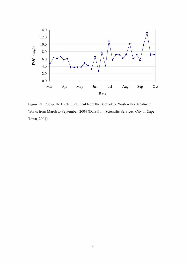
71

0.0

2.0

4.0

6.0

8.0

10.0

12.0

14.0

Mar Apr May Jun Jul Aug Sep Oct

Date

PO43-

(mg/

l)

Figure 21. Phosphate levels in effluent from the Scottsdene Wastewater Treatment

Works from March to September, 2004 (Data from Scientific Services, City of Cape

Town, 2004)

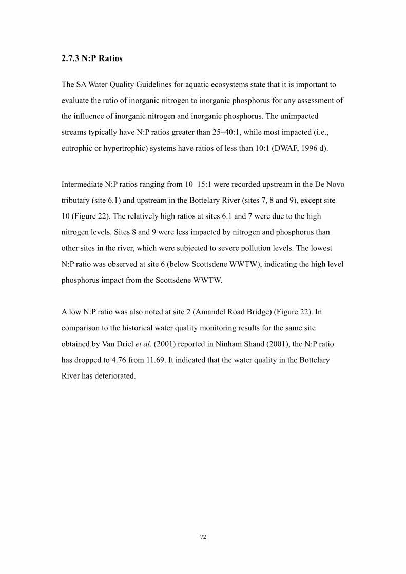
72

2.7.3 N:P Ratios

The SA Water Quality Guidelines for aquatic ecosystems state that it is important to

evaluate the ratio of inorganic nitrogen to inorganic phosphorus for any assessment of

the influence of inorganic nitrogen and inorganic phosphorus. The unimpacted

streams typically have N:P ratios greater than 25–40:1, while most impacted (i.e.,

eutrophic or hypertrophic) systems have ratios of less than 10:1 (DWAF, 1996 d).

Intermediate N:P ratios ranging from 10–15:1 were recorded upstream in the De Novo

tributary (site 6.1) and upstream in the Bottelary River (sites 7, 8 and 9), except site

10 (Figure 22). The relatively high ratios at sites 6.1 and 7 were due to the high

nitrogen levels. Sites 8 and 9 were less impacted by nitrogen and phosphorus than

other sites in the river, which were subjected to severe pollution levels. The lowest

N:P ratio was observed at site 6 (below Scottsdene WWTW), indicating the high level

phosphorus impact from the Scottsdene WWTW.

A low N:P ratio was also noted at site 2 (Amandel Road Bridge) (Figure 22). In

comparison to the historical water quality monitoring results for the same site

obtained by Van Driel et al. (2001) reported in Ninham Shand (2001), the N:P ratio

has dropped to 4.76 from 11.69. It indicated that the water quality in the Bottelary

River has deteriorated.

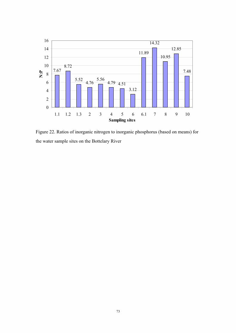
73

7.678.72

5.524.76

5.564.79 4.51

3.12

11.89

14.32

10.95

12.85

7.48

0

2

4

6

8

10

12

14

16

1.1 1.2 1.3 2 3 4 5 6 6.1 7 8 9 10Sampling sites

N:P

Figure 22. Ratios of inorganic nitrogen to inorganic phosphorus (based on means) for

the water sample sites on the Bottelary River

74

2.7.4 Cadmium Concentrations

Cadmium is a heavy metal element and extremely toxic to aquatic organisms. The

sources of cadmium in the aquatic environment are from natural weathering processes,

mining, metal smelters, industries, agricultural use of sludges, fertilizers and

pesticides, burning of fossil fuels, and the deterioration of galvanized materials and

cadmium-plated containers (DWAF, 1996 d).

The cadmium toxicity in water is influenced by water hardness, salinity, chemical

speciation, pH, water temperature, ligands and coexisting metal cations. Cadmium has

a low solubility at neutral or alkaline pH values and is more soluble under acidic

conditions. The toxicity effects of cadmium generally increase as salinity decreases.

The presence of cadmium and other metals may result in either synergistic or

antagonistic interactions; for instance, the interaction of cadmium and copper may

result in a fivefold increase in the toxicity of both metals (DWAF, 1996 d).

The cadmium concentrations in the water samples from the Bottelary River varied

between 0.0521 and 4.4776 µg/l. The mean values of cadmium ranged from 0.2216 to

1.3386 µg/l, with the highest concentrations at site 5 (Groenland Farm) and site 6.1

(concreted canal from Scottsdene). The lowest cadmium value was observed at site 10

(Bottelary Culvert) (Figure 23 A). The results suggest that the main source of

cadmium in the Bottelary River could be urban runoff from Scottsdene.

During the study period, the average cadmium concentrations were in the range of

0.2198–1.4350 µg/l over time and increased (Figure 23B) probably due to increased

runoff because of increased rainfall during wet season (Figure 4).

The SA Target Water Quality Range for cadmium in aquatic ecosystems is below

0.15 µg/l in soft water and less than 0.25 µg/l in moderately soft water. The Chronic

Effect Value for cadmium is 0.3 µg/l in soft water and 0.5 µg/l in moderately soft

75

A

ab

abab

b

abab

ab ab

ab

abab

a a

0.00.2

0.40.6

0.81.0

1.21.4

1.6

1.1 1.2 1.3 2 3 4 5 6 6.1 7 8 9 10Sampling sites

Cd

(µg/

l)

Ba

ababc

bcdcd

d

0.00.2

0.40.60.8

1.01.2

1.41.6

0 50 100 150 200 250 300Time (days)

Cd

(µg/

l)

Figure 23. Means with the same letter are not significantly different at p=0.05.

(A) Cadmium levels (µg/l) at the sampling sites on the Bottelary River over the

sampling period (2004). (B) Seasonal variation of cadmium in the Bottelary River and

its main tributaries.

76

water, while the Acute Effect Value is 3 µg/l in soft water and 6 µg/l in moderately

soft water. The guideline states that ninety percent (90%) of all cadmium

measurements should be within the Target Water Quality Range and “all

measurements should be below the Chronic Effect Value to ensure protection of

aquatic ecosystems” (DWAF, 1996 d).

From the results, only about ten percent (10%) of the cadmium concentrations in the

water samples from the Bottelary River were found within the 0.15 µg/l Target Water

Quality Range for soft water. About twenty-eight percent (28%) of the cadmium

values were observed within the 0.25 µg/l Target Water Quality Range for moderately

soft water. The concentrations of cadmium exceeded the Chronic Effect Value and the

Acute Effect Value in soft water, and the Chronic Effect Value in moderately soft

water. Thus, the cadmium concentrations are unsuitable for sustaining aquatic

ecosystems and the river water could cause adverse chronic and acute effects to

aquatic organisms due to cadmium poisoning.

The cadmium levels detected in the water samples from the Bottelary River were

lower than the SA Water Quality Guideline of 10 µg/l (DWAF, 1996 b&e) in water

for agricultural irrigation. The concentration of cadmium in the river water is suitable

for agricultural irrigation and is not toxic to plants.

The SA Water Quality Guideline for cadmium in water to be used for livestock

watering is 0–10 µg/l (DWAF, 1996 c&e). This level was not exceeded in the water

samples from the Bottelary River. The river water should not lead to adverse chronic

or acute effects of cadmium poisoning in livestock.

77

2.7.5 Copper Concentrations

Copper has been used widely all over the world. It is a micronutrient, which can be

rapidly accumulated by plants and animals. The main sources of copper in the aquatic

environment include geological weathering, corrosion of brass and copper pipes by

acidic waters, sewage treatment plant effluents, copper compounds used as aquatic

algaecides, runoff and groundwater contamination from the use of copper as

fungicides and pesticides, and liquid effluents and atmospheric depositions from

industrial sources (DWAF, 1996 d).

In aquatic ecosystems, copper may be present in the forms of a solution of cupric ions,

complexed with inorganic or organic ligands, associated with suspended or bed

sediments, and as precipitates of hydroxides, phosphates and sulphides. Copper has a

high solubility in acidic waters, and precipitates as copper hydroxides at pH values

greater than 6.5. The toxicity of copper increases in aquatic systems with a decrease in

water hardness, a decrease in dissolved oxygen, and when present in combination

with other metals. Copper toxicity decreases in the presence of chelating agents

(humic acids, amino acids and suspended solids), with an increase in alkalinity, and in

the presence of zinc, molybdenum, sulphate, calcium and magnesium (DWAF, 1996

d).

Copper concentrations in the water samples from the Bottelary River ranged from 0 to

15.6532 µg/l. It was noted that the highest level of copper was 15.6532 µg/l at site 7.1.

Since site 7.1 was an additional small tributary on the Varswater Farm and only ran in

August and September during the sampling period, its mean concentration was not

displayed in Figure 24.

The mean copper values ranged between 2.0364 and 5.3661 µg/l. Low concentrations

of copper were displayed in the Kuils River above the Bottelary River junction (site

1.1), the Swart River (site 8) and on the Mesco Farm (site 9). The highest mean value

78

of copper was observed at site 10 (Bottelary Culvert). The concentrations of copper

also displayed high levels at site 4 (Bottelary Road Bridge) and site 7 (Varswater

Farm) (Figure 24A). The high levels of copper could be attributed to runoff from the

use of copper based pesticides on the farms, and the brick fields upstream of site 10.

Figure 24 (B) shows that average copper concentrations were in the range of

2.5913–3.8333 µg/l and did not differ significantly over the sampling period.

According to the SA Water Quality Guidelines, the Target Water Quality Range for

copper in aquatic ecosystems is less than 0.3 µg/l in soft water and below 0.8 µg/l in

medium soft water. The Chronic Effect Value for copper in water for aquatic

ecosystems is 0.53 µg/l in soft water and 1.5 µg/l in medium soft water, while the

Acute Effect Value for copper is 1.6 µg/l in soft water and 4.6 µg/l in medium soft

water (DWAF, 1996 d). The guideline also states that “ninety percent (90%) of all

dissolved copper measurements for the site in question should be within the Target

Water Quality Range”, while “all measurements should be below the Chronic Effect

Value to ensure protection of aquatic ecosystems” (DWAF, 1996 d).

From the results, only about one percent (1%) of the copper values in the water

samples from the Bottelary River were within the 0.3µg/l Target Water Quality Range

for soft water, while about four percent (4%) were found to be within the 0.8µg/l

Target Water Quality Range for medium soft water. The concentrations of copper in

the water samples from the Bottelary River exceeded the Chronic Effect Value and

the Acute Effect Value for soft and medium soft water. Thus the river water is

unsuitable for aquatic ecosystems and could cause adverse chronic and acute effects

to aquatic organisms due to copper poisoning.

The copper concentrations in the water samples did not exceed the SA Water Quality

Guideline of 200 µg/l (DWAF, 1996 b) in water to be used for agricultural irrigation.

Thus, copper in the river water is suitable for irrigation and is considered safe for

plants.

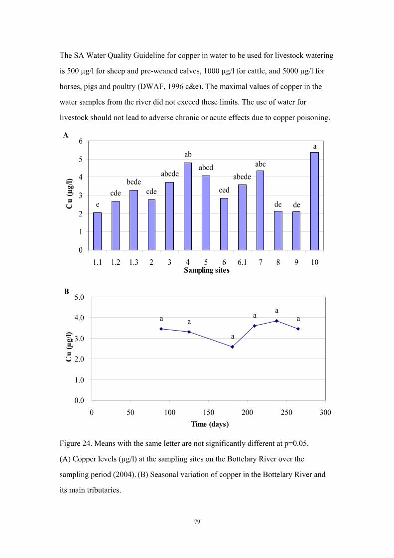
79

The SA Water Quality Guideline for copper in water to be used for livestock watering

is 500 µg/l for sheep and pre-weaned calves, 1000 µg/l for cattle, and 5000 µg/l for

horses, pigs and poultry (DWAF, 1996 c&e). The maximal values of copper in the

water samples from the river did not exceed these limits. The use of water for

livestock should not lead to adverse chronic or acute effects due to copper poisoning.

A

cdededee

cde cedbcde abcdeabcde

abcd abcab

a

0

1

2

3

4

5

6

1.1 1.2 1.3 2 3 4 5 6 6.1 7 8 9 10Sampling sites

Cu

(µg/

l)

B

a a

a

a aa

0.0

1.0

2.0

3.0

4.0

5.0

0 50 100 150 200 250 300Time (days)

Cu

(µg/

l)

Figure 24. Means with the same letter are not significantly different at p=0.05.

(A) Copper levels (µg/l) at the sampling sites on the Bottelary River over the

sampling period (2004). (B) Seasonal variation of copper in the Bottelary River and

its main tributaries.

80

2.7.6 Iron Concentrations

Iron is the fourth most abundant element in the earth's crust and may be present in

natural waters. It is an essential micronutrient for all organisms. Iron is released into

the environment by natural processes, mainly from weathering of sulphide ores and

igneous, sedimentary and metamorphic rocks, and by human activities, mainly from

the burning of coke and coal, acid mine drainage, mineral processing, sewage, landfill

leachates and the corrosion of iron and steel (DWAF, 1996 d).

In the aquatic environment, oxidation-reduction reactions, pH and the presence of

co-existing inorganic and organic complexing agents determine the chemical

behaviour of iron. The iron concentrations may be affected by the biological

interactions in surface waters. The demand for iron during algal blooms can

significantly reduce iron concentrations in the water (DWAF, 1996 d).

The iron values in the water samples varied between 0.0327 and 2.9013 mg/l. The

mean concentrations of iron were in the ranged of 0.1881–0.7491 mg/l. High values

of iron were found upstream in the Bottelary River, including sites 7 (Varswater

Farm), 8 (Swart River), 9 (Mesco Farm) and 10 (Bottelary Culvert) (Figure 25A),

probably due to agricultural runoff and runoff from the brick fields upstream of site

10. Since site 9 was located downstream of site 11 (dam containing winery effluents),

the high iron value at this site could be attributed to the overflow of the dam due to

the high rainfall during the wet season.

Low values of iron were found at sites 1.1 (the Kuils River upstream of the Bottelary

River junction), 2 (Amandel Road Bridge), 5(Groenland Farm) and 6.1(concreted

canal from Scottsdene) (Figure 25A), which indicated these river sections were less

impacted.

During the period of investigation, the mean concentrations of iron were in the range

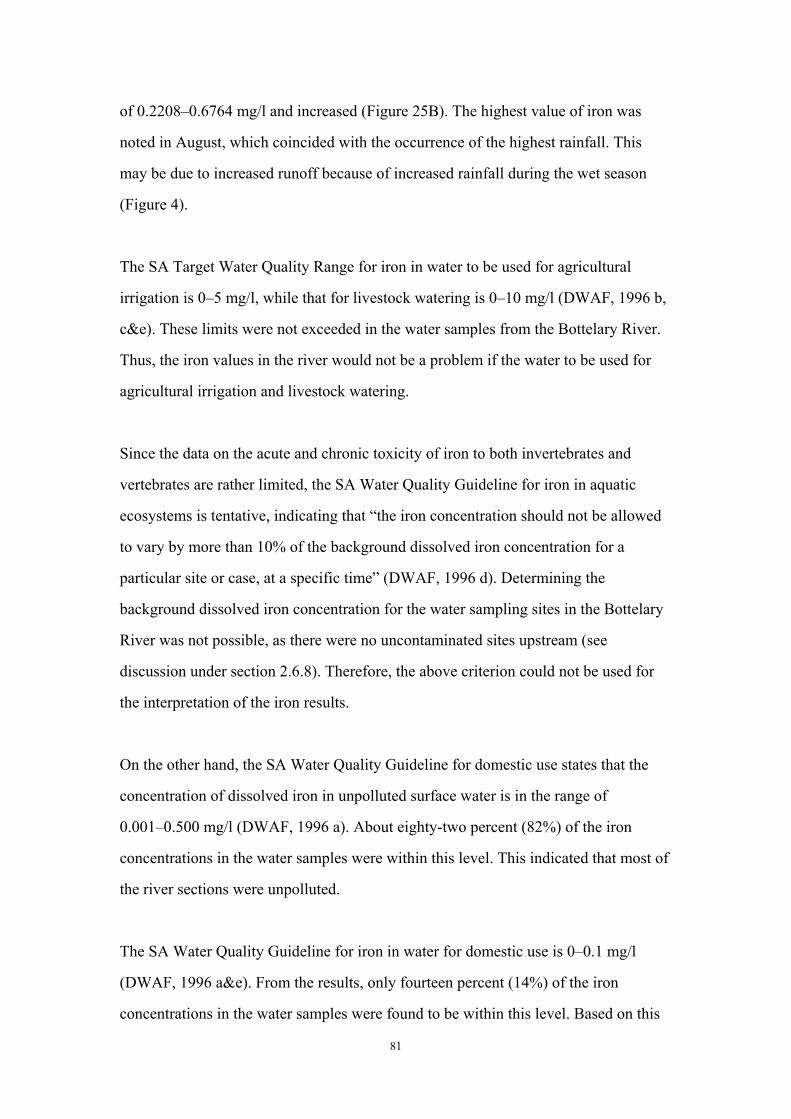
81

of 0.2208–0.6764 mg/l and increased (Figure 25B). The highest value of iron was

noted in August, which coincided with the occurrence of the highest rainfall. This

may be due to increased runoff because of increased rainfall during the wet season

(Figure 4).

The SA Target Water Quality Range for iron in water to be used for agricultural

irrigation is 0–5 mg/l, while that for livestock watering is 0–10 mg/l (DWAF, 1996 b,

c&e). These limits were not exceeded in the water samples from the Bottelary River.

Thus, the iron values in the river would not be a problem if the water to be used for

agricultural irrigation and livestock watering.

Since the data on the acute and chronic toxicity of iron to both invertebrates and

vertebrates are rather limited, the SA Water Quality Guideline for iron in aquatic

ecosystems is tentative, indicating that “the iron concentration should not be allowed

to vary by more than 10% of the background dissolved iron concentration for a

particular site or case, at a specific time” (DWAF, 1996 d). Determining the

background dissolved iron concentration for the water sampling sites in the Bottelary

River was not possible, as there were no uncontaminated sites upstream (see

discussion under section 2.6.8). Therefore, the above criterion could not be used for

the interpretation of the iron results.

On the other hand, the SA Water Quality Guideline for domestic use states that the

concentration of dissolved iron in unpolluted surface water is in the range of

0.001–0.500 mg/l (DWAF, 1996 a). About eighty-two percent (82%) of the iron

concentrations in the water samples were within this level. This indicated that most of

the river sections were unpolluted.

The SA Water Quality Guideline for iron in water for domestic use is 0–0.1 mg/l

(DWAF, 1996 a&e). From the results, only fourteen percent (14%) of the iron

concentrations in the water samples were found to be within this level. Based on this

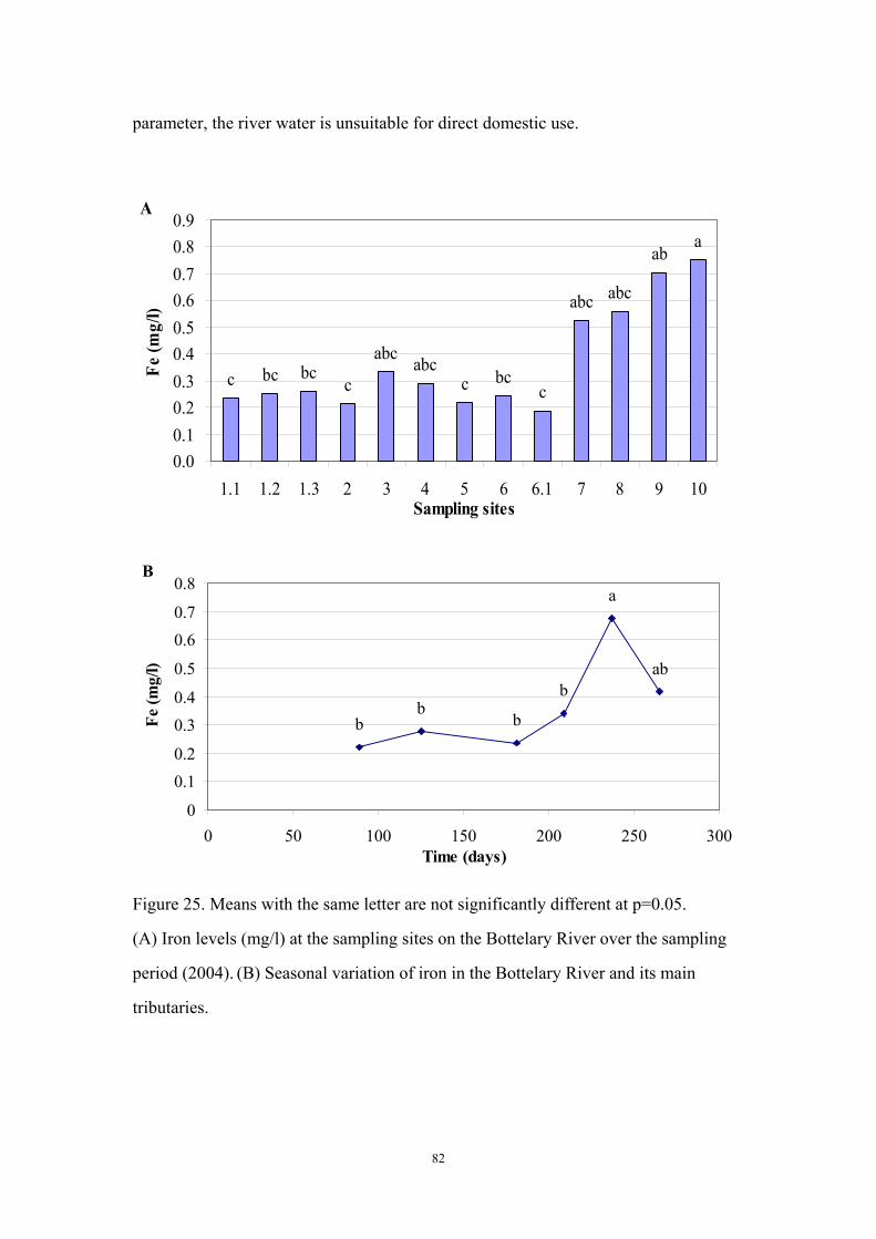
82

parameter, the river water is unsuitable for direct domestic use.

A

abcabc

cbcc bc c bc

c

abc abc

aba

0.00.10.20.30.40.50.60.70.80.9

1.1 1.2 1.3 2 3 4 5 6 6.1 7 8 9 10Sampling sites

Fe (m

g/l)

Ba

abb

bb

b

0

0.10.2

0.30.4

0.5

0.60.7

0.8

0 50 100 150 200 250 300Time (days)

Fe (m

g/l)

Figure 25. Means with the same letter are not significantly different at p=0.05.

(A) Iron levels (mg/l) at the sampling sites on the Bottelary River over the sampling

period (2004). (B) Seasonal variation of iron in the Bottelary River and its main

tributaries.

83

2.7.7 Lead Concentrations

Lead occurs as metallic lead, and inorganic and organometallic compounds, which

readily accumulates in living tissue. It is considered potentially hazardous and toxic to

most forms of life, and relatively accessible to aquatic organisms. The major sources

of lead in the aquatic environment include the weathering of sulphide ores, especially

galena, precipitation, fallout of lead dust, street runoff, industrial and municipal

wastewater discharge, mining, milling and smelting of lead and combustion of fossil

fuels (DWAF, 1996 d).

Lead levels were in the range of 0–0.2686 µg/l in the water samples from the

Bottelary River. The mean values of lead ranged from 0.0232 to 0.1027 µg/l. Figure

26 (A) shows that the highest mean concentration of lead was recorded at site 3,

which was located near the Rainbow Chicken Farm, while the lowest concentrations

of lead were found at site 5 (Groenland Farm) and site 6 (below the Scottsdene

WWTW).

Figure 26 (B) shows that the average concentrations of lead varied erratically between

0.0187 and 0.0968 µg/l, and did not show the increase through to the wet season

reported for many other elements.

According to the SA Water Quality Guidelines for aquatic ecosystems, the Target

Water Quality Range for lead is 0–0.2 µg/l in soft water and 0–0.5 µg/l in medium

soft water. The guideline states that “ninety percent (90%) of all dissolved lead

measurements should be within the Target Water Quality Range” and “all

measurements should be below the Chronic Effect Value to ensure protection of

aquatic ecosystems” (DWAF, 1996 d).

From the results, ninety-five percent (95%) of the lead values in the water samples

were found to be below the 0.2 µg/l Target Water Quality Range for the soft water.

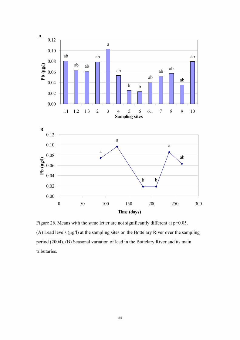
84

A

ab

ababab

bb

ab

ab

ab

abab

ab

a

0.00

0.02

0.04

0.06

0.08

0.10

0.12

1.1 1.2 1.3 2 3 4 5 6 6.1 7 8 9 10Sampling sites

Pb (µ

g/l)

B

a

aa

ab

bb

0.00

0.02

0.04

0.06

0.08

0.10

0.12

0 50 100 150 200 250 300

Time (days)

Pb (µ

g/l)

Figure 26. Means with the same letter are not significantly different at p=0.05.

(A) Lead levels (µg/l) at the sampling sites on the Bottelary River over the sampling

period (2004). (B) Seasonal variation of lead in the Bottelary River and its main

tributaries.

85

None of the lead concentrations exceeded 0.3 µg/l. Since the Chronic Effect Value for

lead in the aquatic ecosystems is 0.5 µg/l in soft water and 1.0 µg/l in medium soft

water (DWAF, 1996 d), these levels were not exceeded in the water samples from the

Bottelary River. The river water is suitable for aquatic ecosystems and no adverse

chronic and acute effects to aquatic organisms would be expected to occur due to lead

poisoning.

The concentrations of lead in the water samples did not exceed the SA Water Quality

Guideline of 200 µg/l (DWAF, 1996 b&e) in water for the use of agricultural

irrigation. Lead is not expected to be a problem in the river water for agricultural

irrigation.

The SA Water Quality Guideline for lead in the water to be used for livestock

watering is 0–500 µg/l for pigs, and 0–100 µg/l for all other livestock (DWAF, 1996

c&e). These levels were not exceeded in the water samples from the Bottelary River.

The use of the river water for livestock watering should not cause adverse chronic

and/or acute effects due to lead poisoning.

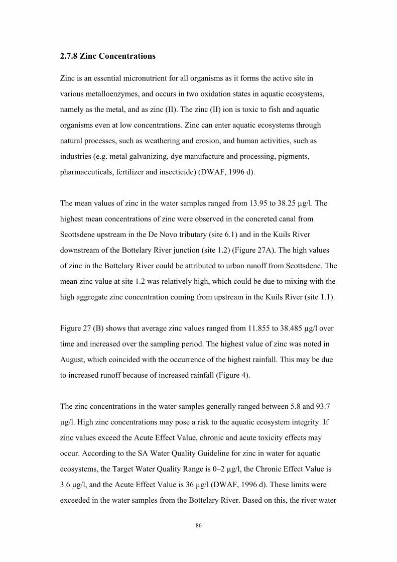
86

2.7.8 Zinc Concentrations

Zinc is an essential micronutrient for all organisms as it forms the active site in

various metalloenzymes, and occurs in two oxidation states in aquatic ecosystems,

namely as the metal, and as zinc (II). The zinc (II) ion is toxic to fish and aquatic

organisms even at low concentrations. Zinc can enter aquatic ecosystems through

natural processes, such as weathering and erosion, and human activities, such as

industries (e.g. metal galvanizing, dye manufacture and processing, pigments,

pharmaceuticals, fertilizer and insecticide) (DWAF, 1996 d).

The mean values of zinc in the water samples ranged from 13.95 to 38.25 µg/l. The

highest mean concentrations of zinc were observed in the concreted canal from

Scottsdene upstream in the De Novo tributary (site 6.1) and in the Kuils River

downstream of the Bottelary River junction (site 1.2) (Figure 27A). The high values

of zinc in the Bottelary River could be attributed to urban runoff from Scottsdene. The

mean zinc value at site 1.2 was relatively high, which could be due to mixing with the

high aggregate zinc concentration coming from upstream in the Kuils River (site 1.1).

Figure 27 (B) shows that average zinc values ranged from 11.855 to 38.485 µg/l over

time and increased over the sampling period. The highest value of zinc was noted in

August, which coincided with the occurrence of the highest rainfall. This may be due

to increased runoff because of increased rainfall (Figure 4).

The zinc concentrations in the water samples generally ranged between 5.8 and 93.7

µg/l. High zinc concentrations may pose a risk to the aquatic ecosystem integrity. If

zinc values exceed the Acute Effect Value, chronic and acute toxicity effects may

occur. According to the SA Water Quality Guideline for zinc in water for aquatic

ecosystems, the Target Water Quality Range is 0–2 µg/l, the Chronic Effect Value is

3.6 µg/l, and the Acute Effect Value is 36 µg/l (DWAF, 1996 d). These limits were

exceeded in the water samples from the Bottelary River. Based on this, the river water

87

Aa

abc

ab

c c cc

abcbc

cc

cc

05

1015202530354045

1.1 1.2 1.3 2 3 4 5 6 6.1 7 8 9 10Sampling sites

Zn

(µg/

l)

B

c cbc

bc b

a

05

1015202530354045

0 50 100 150 200 250 300Time (days)

Zn

(µg/

l)

Figure 27. Means with the same letter are not significantly different at p=0.05.

(A) Zinc levels (µg/l) at the sampling sites on the Bottelary River over the sampling

period (2004). (B) Seasonal variation of zinc in the Bottelary River and its main

tributaries.

88

is unsuitable for aquatic ecosystems and could cause adverse chronic and acute effects

to aquatic organisms due to zinc poisoning.

The SA Water Quality Guideline for zinc in water to be used for agricultural irrigation

is 1000 µg/l and for livestock watering is 20000 µg/l (DWAF, 1996 b, c&e). The zinc

concentrations in the water samples were much lower than these limits. Thus zinc

would not be a problem in the river water to be used for agricultural irrigation and

livestock watering.

89

2.7.9 Electrical Conductivity

The levels of electrical conductivity varied between 0.14 and 5.75 mS/cm in the water

samples from the Bottelary River. The mean values of electrical conductivity ranged

from 0.72 to 3.20 mS/cm and displayed a distinct peak at site 8 (Swart River), while

the lowest electrical conductivity value was observed at site 10 (Bottelary Culvert)

(Figure 28A).

During the period of investigation, the average values of electrical conductivity were

in the range of 1.01–1.41 mS/cm and did not differ significantly (Figure 28B).

The SA Water Quality Guideline for electrical conductivity in water to be used for the

domestic water supply is 70 mS/m (DWAF, 1996 a&e), which is equivalent to 0.7

mS/cm. This limit was exceeded in some of the water samples. Based on this

parameter, the river water is not suitable for direct domestic use.

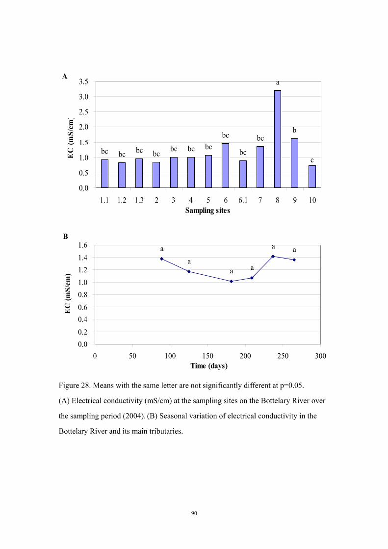
90

Aa

b

cbc bc bc bc bc bc bc

bc

bc

bc

0.0

0.5

1.0

1.5

2.0

2.5

3.0

3.5

1.1 1.2 1.3 2 3 4 5 6 6.1 7 8 9 10Sampling sites

EC

(mS/

cm)

Ba

aa a

a a

0.00.20.40.60.81.01.21.41.6

0 50 100 150 200 250 300Time (days)

EC

(mS/

cm)

Figure 28. Means with the same letter are not significantly different at p=0.05.

(A) Electrical conductivity (mS/cm) at the sampling sites on the Bottelary River over

the sampling period (2004). (B) Seasonal variation of electrical conductivity in the

Bottelary River and its main tributaries.

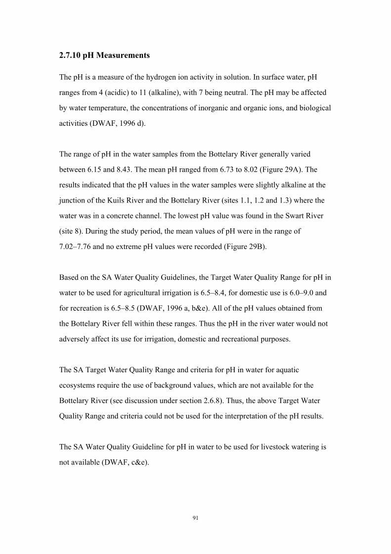
91

2.7.10 pH Measurements

The pH is a measure of the hydrogen ion activity in solution. In surface water, pH

ranges from 4 (acidic) to 11 (alkaline), with 7 being neutral. The pH may be affected

by water temperature, the concentrations of inorganic and organic ions, and biological

activities (DWAF, 1996 d).

The range of pH in the water samples from the Bottelary River generally varied

between 6.15 and 8.43. The mean pH ranged from 6.73 to 8.02 (Figure 29A). The

results indicated that the pH values in the water samples were slightly alkaline at the

junction of the Kuils River and the Bottelary River (sites 1.1, 1.2 and 1.3) where the

water was in a concrete channel. The lowest pH value was found in the Swart River

(site 8). During the study period, the mean values of pH were in the range of

7.02–7.76 and no extreme pH values were recorded (Figure 29B).

Based on the SA Water Quality Guidelines, the Target Water Quality Range for pH in

water to be used for agricultural irrigation is 6.5–8.4, for domestic use is 6.0–9.0 and

for recreation is 6.5–8.5 (DWAF, 1996 a, b&e). All of the pH values obtained from

the Bottelary River fell within these ranges. Thus the pH in the river water would not

adversely affect its use for irrigation, domestic and recreational purposes.

The SA Target Water Quality Range and criteria for pH in water for aquatic

ecosystems require the use of background values, which are not available for the

Bottelary River (see discussion under section 2.6.8). Thus, the above Target Water

Quality Range and criteria could not be used for the interpretation of the pH results.

The SA Water Quality Guideline for pH in water to be used for livestock watering is

not available (DWAF, c&e).

92

A

aabc

ab

de cde cde de ecde cde

f

cde cde

6.0

6.5

7.0

7.5

8.0

8.5

1.1 1.2 1.3 2 3 4 5 6 6.1 7 8 9 10Sampling sites

pH

B

a abab

bcc

d

6.8

7.0

7.2

7.4

7.6

7.8

8.0

0 50 100 150 200 250 300Time (days)

pH

Figure 29. Means with the same letter are not significantly different at p=0.05.

(A) The pH at the sampling sites on the Bottelary River over the sampling period

(2004). (B) Seasonal variation of pH in the Bottelary River and its main tributaries.

93

2.7.11 Dissolved Oxygen Concentrations

Dissolved oxygen is the concentration of free molecular oxygen (a gas) dissolved in

water and is an important element for water quality control. The concentrations of

dissolved oxygen are considered to be the most commonly employed measurement of

the health of aquatic ecosystems and an indicator of a water body’s ability to support

desirable aquatic organisms (Anon., 2004 a).

The dissolved oxygen concentrations are usually close to saturation in unpolluted

surface water, but the excess of saturation (super-saturation of oxygen) indicates

eutrophication in a water body. The solubility of dissolved oxygen in water can be

changed by water temperatures. Higher water temperatures can decrease the dissolved

oxygen concentrations in water and thus its availability to aquatic organisms (DWAF,

1996 d).

The dissolved oxygen concentrations in the water samples from the Bottelary River

ranged between 0.97 and 17.90 mg/l, indicating an oxygen saturation range of

10.6–145.0%. The mean values of dissolved oxygen ranged from 4.07 to 10.87 mg/l,

i.e. oxygen saturation range of 41.80–111.96%.

Figure 30 (A) shows that the mean values of dissolved oxygen in the water samples

were significantly higher at the junction of the Kuils River and the Bottelary River

(sites 1.1, 1.2 and 1.3), while low concentrations of dissolved oxygen were observed

at sites 5 (Groenland Farm), 6 (below the Scottsdene WWTW), and 9 (Mesco Farm).

Figure 30 (B) shows that the mean concentrations of dissolved oxygen were in the

range of 6.01–10.19 mg/l over the sampling period. The highest mean concentration

of dissolved oxygen was noted in July, probably due to the low water temperature

(Figure 31B).

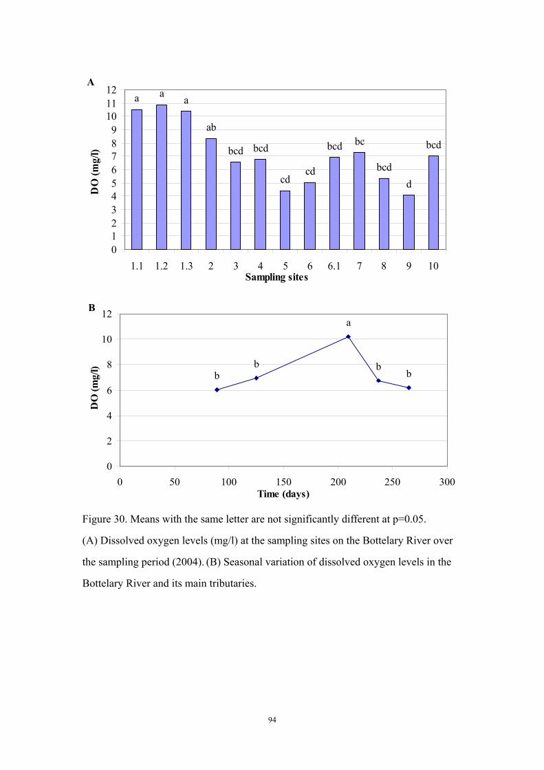
94

A

dcdcd bcd

bcd bcdbcbcdbcd

ab

aaa

0123456789

101112

1.1 1.2 1.3 2 3 4 5 6 6.1 7 8 9 10Sampling sites

DO

(mg/

l)

Ba

bb

bb

0

2

4

6

8

10

12

0 50 100 150 200 250 300Time (days)

DO

(mg/

l)

Figure 30. Means with the same letter are not significantly different at p=0.05.

(A) Dissolved oxygen levels (mg/l) at the sampling sites on the Bottelary River over

the sampling period (2004). (B) Seasonal variation of dissolved oxygen levels in the

Bottelary River and its main tributaries.

95

WHO (1993) as cited by Ngoye and Machiwa (2004) recommended a concentration

of dissolved oxygen of 5 mg/l or above. From the results, about twenty-five percent

(25%) of the dissolved oxygen concentrations in the water samples from the Bottelary

River were less than 5 mg/l. Dissolved oxygen levels below 5 mg/l could cause

adverse affects to aquatic life (Fatoki et al., 2003).

According to the SA Water Quality Guidelines for aquatic ecosystems, the Target

Water Quality Range for dissolved oxygen is 80–120 %. The guideline states that “the

dissolved oxygen concentration must be measured as the lowest instantaneous

concentration recorded in a 24-hour period, or as the instantaneous concentration at

06h00. If dissolved oxygen is measured at some other time of day or night, then

interpretation of the result will require knowledge and understanding of the chemical

and biological conditions at the sampling site over the 24-hour cycle ”(DWAF, 1996

d). Due to the limitations of this study, continual measurement throughout the day

was not possible, thus the SA Water Quality Guidelines for aquatic ecosystems could

not be used for the interpretation of the dissolved oxygen results.

The SA Target Water Quality Range for dissolved oxygen in water to be used for

agricultural irrigation and livestock watering is not available (DWAF, 1996 e).

96

2.7.12 Water Temperature

Temperature plays an important role in water by affecting the rates of chemical

reactions and the metabolic rates of organisms, and controlling the distribution of

aquatic organisms. The changes of water temperature can result from natural

processes, such as climatic and hydrological factors, and anthropogenic sources, such

as discharge of heated effluents, heated return-flows of irrigation water, removal of

riparian vegetation cover (an increase in the amount of solar radiation reaching the

water), inter-basin water transfers, and discharge of water from impoundments

(DWAF, 1996 d).

The water temperature generally ranged from 9.2 to 23.1 ºC. The mean water

temperature varied between 14.4 and 18.6 ºC, while high water temperatures were

found at site 6 (below the Scottsdene WWTW) and at the junction of the Kuils River

and the Bottelary River (sites 1.1, 1.2 and 1.3) (Figure 31A). These river sections

were located at open spaces with less riparian vegetation cover. The lowest mean

water temperature was observed at site 8 (Swart River), which had more riparian

vegetation cover (Figure 14).

Figure 31 (B) shows that the mean water temperatures were in the range of

11.5–19.7 ºC over the sampling period.

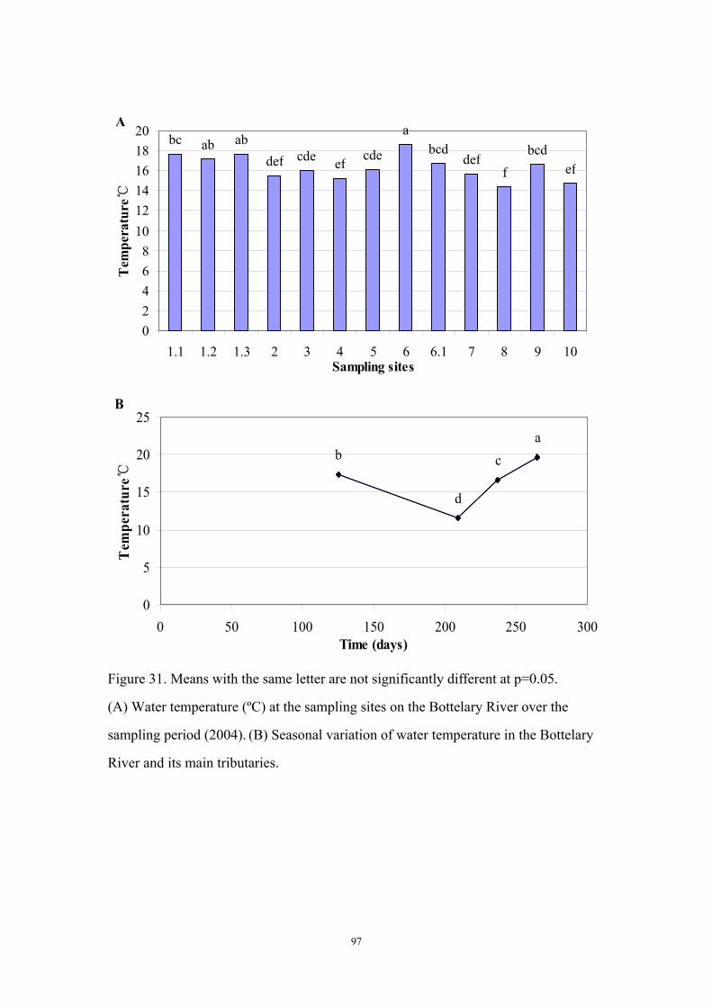
97

A

f efefdef defcde cde bcdbcdbc abab

a

02468

101214161820

1.1 1.2 1.3 2 3 4 5 6 6.1 7 8 9 10Sampling sites

Tem

pera

ture

℃

B

d

cba

0

5

10

15

20

25

0 50 100 150 200 250 300Time (days)

Tem

pera

ture

℃

Figure 31. Means with the same letter are not significantly different at p=0.05.

(A) Water temperature (ºC) at the sampling sites on the Bottelary River over the

sampling period (2004). (B) Seasonal variation of water temperature in the Bottelary

River and its main tributaries.

98

2.7.13 Water Quality in a Dam

Site 11 was in a dam containing the winery effluent, which was only measured once

in September during the study period. The dam is located upstream of site 9 and

downstream of the winery. During the wet season, heavy rainfall could cause the

water overflow from the dam into the river, which would affect the water quality in

the river.

The N:P ratio at site 11 was only 0.52:1, which is below the SA Water Quality

Guideline of 10:1 (DWAF, 1996 d). This indicated that the water in the dam had been

impacted by nitrogen (6.0 mg/l) and phosphate (11.6 mg/l), which can cause

eutrophication. The lowest concentration overall of dissolved oxygen recorded was

0.62 mg/l.

High concentrations of cadmium, copper and zinc in the dam were above the SA

Water Quality Guideline values for aquatic ecosystems. The iron concentration was

also high. The electrical conductivity was 1.7 mS/cm, which is above the SA Water

Quality Guideline value for domestic use. The results showed that water in the dam

could cause adverse chronic and acute effects to aquatic organisms.

The concentrations of cadmium, copper, lead, iron and zinc in the water sample from

the dam were within the SA Water Quality Guideline values for agricultural irrigation

and livestock watering, which indicated that the water in the dam is safe for plants and

livestock.

99

2.8 CONCLUSION

The results showed that the Bottelary River and its tributaries have been chemically

polluted, especially by nitrogen, phosphorus and some heavy metals (cadmium,

copper and zinc). The probable sources of the chemical pollutants in the Bottelary

River include both point sources from the wastewater treatment works, and diffuse

sources from urban runoff and agricultural runoff in the catchment area. However, the

main urban pollution enters the De Novo tributary as a point source (site 6.1).

The concentrations of nitrogen, phosphorus, cadmium, copper and zinc were above

the South African Water Quality Guideline values for aquatic ecosystems in the

Bottelary River and the dam below the winery, which may adversely affect the health

of aquatic ecosystems. The pH and lead levels were within the South African

guidelines for aquatic ecosystems. The values of electrical conductivity, nitrate and

iron in the water samples were above guideline values for domestic use. There was no

salinity problem in the Bottelary River system as shown by the low levels of electrical

conductivity obtained, except in the Swart River.

During the period of investigation, the increasing concentrations of nitrate, nitrite,

ammonium ion, total nitrogen, phosphate, cadmium, iron and zinc are thought to be

due to the increased load in the runoff because of the rainfall during the wet winter

season.

The high values of nitrogen and phosphorus would be very harmful to the aquatic

ecosystems, as it would encourage eutrophication in the Bottelary River and the dam,

especially in the De Novo tributary. The N:P ratios showed that the water in the

middle and lower part of the Bottelary River was in the hypertrophic condition.

The levels of cadmium, copper, lead, iron, and zinc were within the South African

Water Quality Guidelines for water uses for agricultural irrigation and livestock

100

watering. At these levels of concentrations, the use of the water for plants and

livestock may not lead to toxicity.

101

2.9 REFERENCES

Allen, S.E., Grimshaw, H.M. & Rowland, A.P. (1986). Chemical analysis. Moore, P.D.

& Chapman, S.B. (eds.), Methods in plant ecology. Oxford: Blackwell Scientific.

Alloway, B.J. & Ayres, D.C. (1997). Chemical principles of environmental pollution.

2nd ed. London: Blackie.

Anonymous (2004 a). Dissolved Oxygen. [Online]. Available

http://www.waterontheweb.org/under/waterquality/oxygen.html (downloaded in

December 2004).

Anonymous (2004 b). South Africa at a Glance. [Online]. Available

http://www.forestry.co.za/fsa/showContent.do?content_id=41 (downloaded in March

2005).

Baird, C. & Cann, M. (2005). Environmental chemistry. 3rd ed. New York: W.H.

Freeman and Company.

Cape Wastewater Consultants (1999). Strategic evaluation of bulk wastewater:

Scottsdene Wastewater Treatment Works. Report No.14 to the Cape Metropolitan

Council.

Causapé, J., Quílez, D. & Aragüés, R. (2004). Assessment of irrigation and

environmental quality at the hydrological basin level II: salt and nitrate loads in

irrigation return flows. Agricultural Water Management, 70: 211–228.

Davies, B. & Day, J. (1998). Vanishing waters. Cape Town: University of Cape Town

Press.

102

DWAF (1996 a). South African Water Quality Guidelines, Volume 1: Domestic Use.

2nd ed. Pretoria: Department of Water Affairs and Forestry.

DWAF (1996 b). South African Water Quality Guidelines, Volume 4: Agricultural

Use: Irrigation. 2nd ed. Pretoria: Department of Water Affairs and Forestry.

DWAF (1996 c). South African Water Quality Guidelines, Volume 5: Agricultural

Use: Livestock Watering. 2nd ed. Pretoria: Department of Water Affairs and Forestry.

DWAF (1996 d). South African Water Quality Guidelines, Volume 7: Aquatic

Ecosystem Use. Pretoria: Department of Water Affairs and Forestry.

DWAF (1996 e). South African Water Quality Guidelines, Volume 8: Field Guideline.

Pretoria: Department of Water Affairs and Forestry.

Fatoki, O.S., Gogwana, P. & Ogunfowokan, A.O. (2003). Pollution assessment in the

Keiskamma River and in the impoundment downstream. Water SA, 29: 183–187.

Fatoki, O.S., Muyima, N.Y.O. & Lujiza, N. (2001). Situation analysis of water quality

in the Umtata River catchment. Water SA, 27: 467–473.

Haslam, S.M. (1995). River pollution: an ecological perspective. Chichester: Wiley.

Meyer, N. (2003). Water quality management in the Kuils River. (Cape Metropolitan

Council). Cape Town: Seminar presented at University of the Western Cape.

Murphy, J. & Riley, J.P. (1962). A modified single solution method for the

determination of phosphate in natural waters. Analytica Chimica Acta, 27: 31–36.

Ngoye, E. & Machiwa, J.F. (2004). The influence of land-use patterns in the Ruvu

103

River watershed on water quality in the river system. Physics and Chemistry of the

Earth, 29: 1161–1166.

Ninham Shand (1979). Flow in the Kuils River and drainage of the catchment. Report

No. 543/3200. Cape Town: Ninham Shand Inc.

Ninham Shand (1994). Final report: Kuils River environmental management study.

Report No. 2194/6124. Western Cape Regional Services Council.

Ninham Shand (2001). Upgrading of the Bottelary River between School Street and

Amandel Drive: Draft scoping report. Report No. 3181/9045. Cape Town: Ninham

Shand Inc.

Ninham Shand & Chittenden Nicks (1999). Kuils River Metropolitan Open Space

System (MOSS). Volume 1-Final Report. Report No. 2913. Cape Town: Ninham

Shand Inc.

SAS (1999). SAS/Stat User’s Guide. version 8.2. Volume 2. SAS Campus drive, Cary,

North Carolina 27513: SAS Institute Inc.

van Driel, D. (2003). Assessment of the Scottsdene Wastewater Treatment Works

impacts on the Bottelary River. Unpublished paper. City of Cape Town: Scientific

Services.

WHO (2004). Guidelines for Drinking Water Quality. Volume 1: Recommendations.

3rd ed. Geneva: World Health Organization.

Withers, P.J.A. & Lord, E.I. (2002). Agricultural nutrient inputs to rivers and

groundwaters in the UK: policy, environmental management and research needs. The

104

Science of the Total Environment, 282–283: 9–24.

105

CHAPTER 3

Summary and Recommendations

106

3.1 SUMMARY

Chemical pollution of freshwater is a worldwide environmental problem;

eutrophication, heavy metals and salinity are amongst the most widely used indicators

of pollution. The aim of the study was to assess the status of nutrients, heavy metals

and salinity, and their seasonal variation in the Bottelary River. The results showed

that the water quality in the Bottelary River has deteriorated due to inorganic

chemical pollutants, especially nitrogen, phosphorus, cadmium, copper and zinc. The

main sources of inorganic chemical pollution in the Bottelary River include both

diffuse sources from urban and agricultural runoff, and point source discharge from

the Scottsdene WWTW, Scottsdene, and Kraaifontein.

The high concentrations of nitrate, nitrite, ammonium ion, phosphate, cadmium,

copper, and zinc in the water samples from the Bottelary River were observed to be

above the Target Water Quality Range when compared to the South African Water

Quality Guidelines for aquatic ecosystems (DWAF, 1996 b), which may adversely

affect the health of the aquatic ecosystems. The excessive nitrogen and phosphorus

would cause eutrophication in the Bottelary River. The pH and lead levels were

within the guideline recommendations. The values of electrical conductivity, nitrate

and iron in the water samples were above guideline values for domestic use. There

was no salinity problem in the river as revealed by the low levels of electrical

conductivity.

The major sources, that caused the high values, of nitrogen, phosphorus, cadmium and

zinc in the Bottelary River were from the De Novo tributary. The urban runoff in the

concreted canal from Scottsdene contained high levels of nitrate, nitrite, ammonium

ion, total nitrogen, cadmium and zinc. The high values of phosphorus that were found

downstream in the De Novo tributary, were attributed to the effluent discharge from

the Scottsdene WWTW. Agricultural runoff also significantly contributed to high

concentrations of nitrogen and heavy metals in the Bottelary River.

107

The increased concentrations of nutrients, cadmium, iron, and zinc over the study

period are thought to be primarily derived from the additional input of these

constituents from agricultural and urban runoff because of increased rainfall during

the wet winter season. During the heavy rainfall, runoff increased very rapidly. The

large amounts of water containing nutrients and metal compounds were transported

via surface and subsurface runoff from the farmlands into the river. The increased

concentrations of heavy metals in the river water could also have been due to

increased suspension of sediments that entered the river through agricultural and

urban runoff.

The levels of cadmium, copper, iron, lead, and zinc in the water samples from the

Bottelary River were within the South African Water Quality Guidelines values for

water uses for agricultural irrigation and livestock watering. The water use may not

lead to metals toxicity to plants and livestock.

108

3.2 RECOMMENDATIONS

The chemical composition of the water in the Bottelary River and its tributaries were

greatly effected by agricultural management practices, urban pollution, the Scottsdene

WWTW and climatic conditions in the catchment area. The main source of water

pollution for the Bottelary River is the De Novo tributary, which receives urban runoff,

agricultural runoff, and effluents from the Scottsdene WWTW. It is thus important

that more attention be given to the De Novo tributary in terms of management

interventions due to its high concentrations of nutrients (nitrogen compounds and

phosphorus) and heavy metals (cadmium and zinc).

It is recommended that the impact of urban runoff should be reduced by a number of

options for which the following could be considered:

• Planting of a riparian buffer zone

• Creating runoff containment zones

• An expanded wetland in the lower reaches of the De Novo tributary would

probably solve the problem. This would also be good for wildlife.

The impacts of agricultural runoff could be ameliorated through the encouragement of

farmers to practice Best Management Practices (BMP) on their farms. Some

suggested solutions may include the creation of water collection ponds on the edges

of the fields to trap the runoff, which would then be allowed to enter the river once the

levels of nutrients and heavy metals have been reduced. Furthermore, farmers within

the catchment area should be encouraged to rationalize the fertilizer applications to

reduce the input of nutrients and heavy metals from the farmlands into the river

through runoff.

It is further recommended that the development of “constructed wetlands” to treat

urban storm runoff and agricultural runoff should be considered. The practice which

many farmers have of collecting drainage water and reusing it (Jordens, pers. comm.,

109

2005) should be encouraged.

The treated sewage effluent from the Scottsdene WWTW generally causes the adverse

impacts on water quality in the De Novo tributary and the Bottelary River. This point

source pollution could be reduced by upgrading the sewage treatment works to

improve its treatment performance and by reducing the input of treated sewage

effluent to the river through encouraging its direct use for agricultural irrigation.

It was noted by van Driel (2003) that the Department of Water Affairs and Forestry, in

their license conditions for effluent quality, have set no maximum permissible level

for nitrogen and phosphorus probably due to current financial reality. This does not

allow for upgrading of the works to give a decisively improved aquatic environment.

However, limits still need to be set for the nutrient content of Scottsdene effluent by

local and central authorities.

It is further recommended that the Cape Metropolitan Council (CMC) should develop

Total Maximum Daily Loads (TMDL) for all receiving waters especially for urban

rivers taking into consideration the fact that each water resource has different use

category and therefore may require differential treatment.

A major use of water from the Bottelary River is for agricultural irrigation by local

farmers; the high levels of nitrogen and heavy metals in the river water are of great

concern. On-farm management practices available to mitigate elevated nitrogen levels

in irrigation water (DWAF, 1996 a), are to:

• reduce nitrogen fertilizer application by the amount added with irrigation

water;

• dilute the nitrogen-rich source if alternative water source is available;

• use the nitrogen-rich source only during vegetative plant growth stages;

• change to crops with a high nitrogen requirement;

• use a water source that is low in nitrogen during periods when crop nitrogen

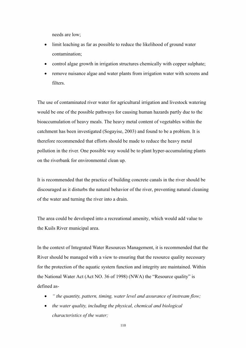
110

needs are low;

• limit leaching as far as possible to reduce the likelihood of ground water

contamination;

• control algae growth in irrigation structures chemically with copper sulphate;

• remove nuisance algae and water plants from irrigation water with screens and

filters.

The use of contaminated river water for agricultural irrigation and livestock watering

would be one of the possible pathways for causing human hazards partly due to the

bioaccumulation of heavy meals. The heavy metal content of vegetables within the

catchment has been investigated (Sogayise, 2003) and found to be a problem. It is

therefore recommended that efforts should be made to reduce the heavy metal

pollution in the river. One possible way would be to plant hyper-accumulating plants

on the riverbank for environmental clean up.

It is recommended that the practice of building concrete canals in the river should be

discouraged as it disturbs the natural behavior of the river, preventing natural cleaning

of the water and turning the river into a drain.

The area could be developed into a recreational amenity, which would add value to

the Kuils River municipal area.

In the context of Integrated Water Resources Management, it is recommended that the

River should be managed with a view to ensuring that the resource quality necessary

for the protection of the aquatic system function and integrity are maintained. Within

the National Water Act (Act NO. 36 of 1998) (NWA) the “Resource quality” is

defined as-

• “ the quantity, pattern, timing, water level and assurance of instream flow;

• the water quality, including the physical, chemical and biological

characteristics of the water;

111

• the characteristics and condition of the instream and riparian habitat; and

• the characteristics, condition and distribution of the aquatic biota”(RSA,

1998).

The NWA requires that all rivers be assessed with a view to classifying them into

classes representing different levels of protection required for their management. The

system of classification of water resources as provided for by the NWA assigns a class

based on the degree of impact of the river-from extremely impacted (Class E or F) to

those that are largely natural (Class A) (DWAF, 1999; Malan et al., 2003). It is

therefore recommended that the Bottelary River should be classified so that

appropriate management intervention could be made.

The Cape Metropolitan Council should be encouraged to develop plans for the

rehabilitation of the Bottelary River to guarantee improved and protected water

quality. After the rehabilitation, management guidelines should be developed for the

river. These management guidelines, based on Integrated Water Resources

Management principles, should inform the management practices to be adopted.

112

3.3 REFERENCES

DWAF (1996 a). South African Water Quality Guidelines, Volume 4: Agricultural

Use: Irrigation. 2nd ed. Pretoria: Department of Water Affairs and Forestry.

DWAF (1996 b). South African Water Quality Guidelines, Volume 7: Aquatic

Ecosystem Use. Pretoria: Department of Water Affairs and Forestry.

DWAF (1999). Resource Directed Measures for Protection of Water Resources.

Volume 2: Integrated Manual Version. Pretoria: Department of Water Affairs and

Forestry.

Malan, H., Bath, A., Day, J. & Joubert, A. (2003). A simple flow-concentration

modeling method for integrating water quality and water quantity in rivers. Water SA,

29: 305–312.

Republic of South Africa (1998). The National Water Act, Act 36 of 1998. The

Department of Water Affairs and Forestry. Government Gazette, Volume 398, No

19182, 26 August 1998. Cape Town: Government Printer.

Sogayise, M. (2003). Contamination of vegetables with heavy metals. Unpublished

Honors Project, Department of Biodiversity and Conservation Biology. Cape Town:

University of the Western Cape.

van Driel, D. (2003). Assessment of the Scottsdene Wastewater Treatment Works

impacts on the Bottelary River. Unpublished paper. City of Cape Town: Scientific

Services.

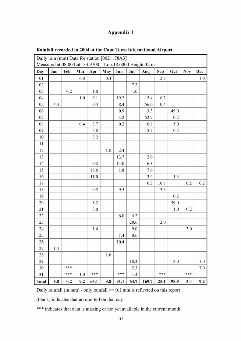
113

Appendix 1

Rainfall recorded in 2004 at the Cape Town International Airport.

Daily rain (mm) Data for station [0021178A3] Measured at 08:00 Lat:-33.9700 Lon:18.6000 Height:42 m Day Jan Feb Mar Apr May Jun Jul Aug Sep Oct Nov Dec

01 6.8 0.4 2.5 1.002 7.2 03 0.2 1.0 1.0 04 1.0 9.1 19.2 15.4 6.2 05 4.4 0.4 8.4 56.0 0.4 06 0.9 3.3 49.0 07 3.2 52.9 0.2 08 0.4 3.7 0.2 6.8 5.0 09 2.8 15.7 0.2 10 3.2 11 12 1.8 2.4 13 13.7 2.0 14 0.2 14.0 6.3 15 18.6 1.8 7.6 16 11.0 3.4 1.3 17 0.3 10.7 0.2 0.218 0.5 9.5 3.3 19 0.2 20 8.2 39.0 21 3.0 1.0 0.2 22 6.0 4.2 23 20.6 2.0 24 1.4 9.0 3.0 25 1.4 0.6 26 10.4 27 1.4 28 1.6 29 18.4 3.0 1.030 *** 2.3 7.031 *** 1.0 *** *** 1.4 *** ***

Total 5.8 0.2 9.2 63.1 3.8 91.1 64.7 169.7 25.1 98.9 3.4 9.2

Daily rainfall (in mm) - only rainfall >= 0.1 mm is reflected on this report

(blank) indicates that no rain fell on that day

*** indicates that data is missing or not yet available in the current month

114

Appendix 2

The Bottelary River water analyses: raw data

Site Distance

(km)

Date Day of

Year

DO

(mg/l)

DO

(%)

pH Temp

(oC)

EC

(mS/cm)

NO3-

(mg/l)

NO2-

(mg/l)

NH4+

(mg/l)

TN

(mg/l)

PO43-

(mg/l)

Cd

(µg/l)

Cu

(µg/l)

Pb

(µg/l)

Zn

(µg/l)

Fe

(mg/l)

1.1 0.00 29.03.04 89 6.10 66.50 7.24 . 0.90 0.0 0.025 0.250 0.275 0.0211 0.0731 2.3928 0.0748 7.1 0.1225

1.2 0.00 29.03.04 89 7.35 80.50 7.26 . 1.56 0.0 0.025 0.250 0.275 1.4229 0.2354 0.6647 0.0934 5.8 0.1262

1.3 0.00 29.03.04 89 13.00 145.00 8.27 . 0.98 2.5 0.000 0.250 2.750 0.1974 0.1992 1.8694 0.1495 12.4 0.2376

2 1.15 29.03.04 89 3.48 35.80 6.46 . 0.52 10.0 0.000 0.250 10.250 0.0000 0.0905 1.8112 0.1308 11.0 0.0327

3 3.55 29.03.04 89 3.58 37.10 6.25 . 1.39 0.0 0.000 0.250 0.250 0.0000 0.3375 1.6118 0.2243 11.1 0.5428

4 5.10 29.03.04 89 6.89 67.20 7.17 . 1.53 40.0 0.050 0.500 40.550 7.7708 0.0521 5.0681 0.0000 10.2 0.1379

5 6.50 29.03.04 89 3.41 34.70 7.06 . 1.72 80.0 0.050 0.500 80.550 13.8370 0.2719 4.9435 0.0000 9.0 0.0337

6 8.65 29.03.04 89 5.13 58.30 7.20 . 0.58 10.0 1.000 7.500 18.500 21.3130 0.2307 3.2237 0.0000 11.3 0.3862

6.1 9.50 29.03.04 89 . . . . . . . . . . . . . . .

7 8.75 29.03.04 89 6.74 71.70 7.18 . 1.39 100.0 0.025 0.500 100.525 5.0994 0.3315 3.6806 0.0000 10.5 0.0348

7.1 8.75 29.03.04 89 . . . . . . . . . . . . . . .

8 11.50 29.03.04 89 2.46 25.60 6.15 . 4.35 0.0 0.000 0.250 0.250 0.0000 0.3355 0.5567 0.0000 10.1 0.1110

9 11.20 29.03.04 89 . . . . . . . . . . . . . .

10 10.75 29.03.04 89 8.04 83.20 7.19 . 0.14 2.5 0.000 0.250 2.750 0.0000 0.2604 12.0649 0.1429 31.9 0.6638

11 . 29.03.04 89 . . . . . . . . . . . . . . .

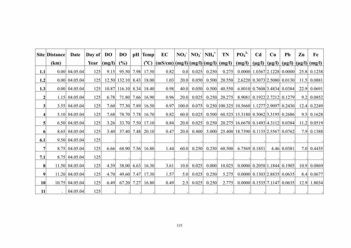
115

Site Distance

(km)

Date Day of

Year

DO

(mg/l)

DO

(%)

pH Temp

(oC)

EC

(mS/cm)

NO3-

(mg/l)

NO2-

(mg/l)

NH4+

(mg/l)

TN

(mg/l)

PO43-

(mg/l)

Cd

(µg/l)

Cu

(µg/l)

Pb

(µg/l)

Zn

(µg/l)

Fe

(mg/l)

1.1 0.00 04.05.04 125 9.15 95.50 7.98 17.50 0.82 0.0 0.025 0.250 0.275 0.0000 1.0367 2.1228 0.0000 25.8 0.1238

1.2 0.00 04.05.04 125 12.50 132.10 8.43 18.00 1.03 20.0 0.050 0.500 20.550 2.6220 0.3073 2.5080 0.0130 11.5 0.0881

1.3 0.00 04.05.04 125 10.87 116.10 8.34 18.40 0.98 40.0 0.050 0.500 40.550 6.8010 0.7608 3.4834 0.0384 22.9 0.0691

2 1.15 04.05.04 125 6.78 71.80 7.66 16.90 0.96 20.0 0.025 0.250 20.275 8.9081 0.1922 2.7212 0.1279 9.2 0.0852

3 3.55 04.05.04 125 7.60 77.30 7.89 16.50 0.97 100.0 0.075 0.250 100.325 10.5660 1.1277 2.9097 0.2430 12.4 0.2249

4 5.10 04.05.04 125 7.68 78.70 7.78 16.70 0.82 60.0 0.025 0.500 60.525 15.3180 0.3062 3.3195 0.2686 9.5 0.1628

5 6.50 04.05.04 125 3.26 33.70 7.50 17.10 0.84 20.0 0.025 0.250 20.275 16.6670 0.1493 4.3112 0.0384 11.2 0.0519

6 8.65 04.05.04 125 3.40 37.40 7.48 20.10 0.47 20.0 0.400 5.000 25.400 18.7390 0.1135 2.5567 0.0762 7.9 0.1388

6.1 9.50 04.05.04 125 . . . . . . . . . . . . . . .

7 8.75 04.05.04 125 6.66 68.90 7.56 16.80 1.44 60.0 0.250 0.250 60.500 6.7569 0.1851 4.46 0.0381 7.0 0.4435

7.1 8.75 04.05.04 125 . . . . . . . . . . . . . . .

8 11.50 04.05.04 125 4.39 38.00 6.63 16.30 3.61 10.0 0.025 0.000 10.025 0.0000 0.2058 1.1844 0.1905 10.9 0.0869

9 11.20 04.05.04 125 4.70 49.60 7.47 17.30 1.57 5.0 0.025 0.250 5.275 0.0000 0.1303 2.8835 0.0635 8.4 0.0677

10 10.75 04.05.04 125 6.49 67.20 7.27 16.80 0.49 2.5 0.025 0.250 2.775 0.0000 0.1535 7.1147 0.0635 12.9 1.8034

11 . 04.05.04 125 . . . . . . . . . . . . . . .

116

Site Distance

(km)

Date Day of

Year

DO

(mg/l)

DO

(%)

pH Temp

(oC)

EC

(mS/cm)

NO3-

(mg/l)

NO2-

(mg/l)

NH4+

(mg/l)

TN

(mg/l)

PO43-

(mg/l)

Cd

(µg/l)

Cu

(µg/l)

Pb

(µg/l)

Zn

(µg/l)

Fe

(mg/l)

1.1 0.00 29.06.04 181 . . 7.92 . 0.60 5.0 0.025 0.500 5.525 0.0000 1.2610 3.1122 0.0644 45.7 0.2383

1.2 0.00 29.06.04 181 . . 7.78 . 0.76 40.0 0.025 0.025 40.050 1.5905 0.4921 2.7364 0.0773 24.1 0.2120

1.3 0.00 29.06.04 181 . . 7.86 . 1.15 60.0 0.025 0.500 60.525 7.2154 0.5348 3.0223 0.0000 16.4 0.1893

2 1.15 29.06.04 181 . . 7.56 . 0.91 60.0 0.025 0.500 60.525 8.0353 0.5890 0.0000 0.0000 15.3 0.1636

3 3.55 29.06.04 181 . . 7.77 . 0.98 60.0 0.025 1.000 61.025 8.7318 0.8945 2.7528 0.0000 15.9 0.2462

4 5.10 29.06.04 181 . . 7.64 . 0.94 60.0 0.025 1.000 61.025 10.4590 0.3085 3.3233 0.0000 10.6 0.1996

5 6.50 29.06.04 181 . . 7.36 . 0.94 40.0 0.075 0.500 40.575 11.5710 0.9790 3.3968 0.0000 13.6 0.0836

6 8.65 29.06.04 181 . . 7.44 . 0.52 50.0 0.500 3.000 53.500 9.1550 0.7024 2.0658 0.0000 21.6 0.2749

6.1 9.50 29.06.04 181 . . 7.58 . 0.90 80.0 0.600 5.000 85.600 7.3035 0.3352 2.3924 0.0000 14.8 0.2444

7 8.75 29.06.04 181 . . 7.46 . 1.31 80.0 0.050 1.000 81.050 4.3588 0.2546 3.7152 0.0000 7.7 0.3242

7.1 8.75 29.06.04 181 . . . . . . . . . . . . . . .

8 11.50 29.06.04 181 . . 6.67 . 2.21 5.0 0.025 0.500 5.525 0.4884 0.1193 0.8002 0.0000 16.8 0.2742

9 11.20 29.06.04 181 . . 7.41 . 1.39 0.0 0.075 0.500 0.575 0.0000 0.3119 1.0860 0.0000 13.5 0.0669

10 10.75 29.06.04 181 . . 6.86 . 0.56 0.0 0.025 0.500 0.525 0.0000 0.2759 5.2830 0.1009 8.5 0.5771

11 . 29.06.04 181 . . . . . . . . . . . . . . .

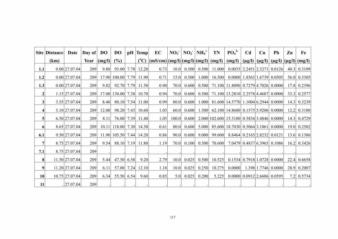
117

Site Distance

(km)

Date Day of

Year

DO

(mg/l)

DO

(%)

pH Temp

(oC)

EC

(mS/cm)

NO3-

(mg/l)

NO2-

(mg/l)

NH4+

(mg/l)

TN

(mg/l)

PO43-

(mg/l)

Cd

(µg/l)

Cu

(µg/l)

Pb

(µg/l)

Zn

(µg/l)

Fe

(mg/l)

1.1 0.00 27.07.04 209 9.80 93.00 7.78 12.20 0.73 10.0 0.500 0.500 11.000 0.0035 2.2451 2.3271 0.0126 40.3 0.3109

1.2 0.00 27.07.04 209 17.90 100.00 7.79 11.90 0.71 15.0 0.500 1.000 16.500 0.0000 1.8563 1.6739 0.0505 56.0 0.3305

1.3 0.00 27.07.04 209 9.82 92.70 7.79 11.50 0.90 70.0 0.600 0.500 71.100 11.8090 0.7279 4.7026 0.0000 17.8 0.2396

2 1.15 27.07.04 209 17.00 130.00 7.38 10.70 0.94 70.0 0.600 0.500 71.100 13.2810 2.2578 4.4687 0.0000 33.3 0.2577

3 3.55 27.07.04 209 8.40 80.10 7.54 11.00 0.99 80.0 0.600 1.000 81.600 14.5770 1.1004 6.2944 0.0000 14.3 0.3239

4 5.10 27.07.04 209 12.00 98.20 7.43 10.60 1.03 60.0 0.600 1.500 62.100 14.8680 0.1575 5.9206 0.0000 12.2 0.3180

5 6.50 27.07.04 209 8.11 76.00 7.39 11.40 1.05 100.0 0.600 2.000 102.600 15.3180 0.5834 3.4846 0.0000 14.3 0.4729

6 8.65 27.07.04 209 10.11 118.00 7.30 14.30 0.61 80.0 0.600 5.000 85.600 18.7030 0.5064 3.1861 0.0000 19.0 0.2502

6.1 9.50 27.07.04 209 11.90 105.50 7.44 14.20 0.86 90.0 0.600 9.000 99.600 8.8464 0.2165 2.8232 0.0121 13.6 0.1386

7 8.75 27.07.04 209 9.54 88.10 7.19 11.80 1.19 70.0 0.100 0.500 70.600 7.0479 0.4837 6.3965 0.1086 16.2 0.3426

7.1 8.75 27.07.04 209 . . . . . . . . . . . . . . .

8 11.50 27.07.04 209 5.44 47.50 6.58 9.20 2.79 10.0 0.025 0.500 10.525 0.1534 0.7918 1.0728 0.0000 22.4 0.6658

9 11.20 27.07.04 209 6.11 57.00 7.24 12.10 1.18 10.0 0.025 0.250 10.275 0.0000 1.398 1.7746 0.0000 28.9 0.2007

10 10.75 27.07.04 209 6.34 55.50 6.54 9.60 0.85 5.0 0.025 0.200 5.225 0.0000 0.0912 2.6686 0.0595 7.2 0.5734

11 . 27.07.04 209 . . . . . . . . . . . . . . .

118

Site Distance

(km)

Date Day of

Year

DO

(mg/l)

DO

(%)

pH Temp

(oC)

EC

(mS/cm)

NO3-

(mg/l)

NO2-

(mg/l)

NH4+

(mg/l)

TN

(mg/l)

PO43-

(mg/l)

Cd

(µg/l)

Cu

(µg/l)

Pb

(µg/l)

Zn

(µg/l)

Fe

(mg/l)

1.1 0.00 24.08.04 237 13.06 140.40 8.37 18.60 0.86 5.0 0.075 0.100 5.175 2.8424 2.1923 1.9953 0.2143 47.2 0.2939

1.2 0.00 24.08.04 237 11.70 123.30 7.98 17.90 0.82 40.0 0.020 0.100 40.120 7.8678 1.295 3.2039 0.0834 22.8 0.3581

1.3 0.00 24.08.04 237 9.99 104.90 7.97 17.50 0.82 30.0 0.050 0.150 30.200 12.3380 0.4825 3.3905 0.1191 28.9 0.4577

2 1.15 24.08.04 237 8.21 82.70 7.80 15.70 0.80 30.0 0.050 0.200 30.250 13.7480 1.0782 3.2769 0.1548 24.1 0.3791

3 3.55 24.08.04 237 6.94 69.90 7.79 15.80 0.83 30.0 0.100 0.200 30.300 15.0180 1.9167 4.5260 0.1004 36.1 0.3807

4 5.10 24.08.04 237 3.62 36.20 7.45 15.70 0.82 60.0 0.700 0.300 61.000 16.1730 0.6984 7.0892 0.0502 23.5 0.4483

5 6.50 24.08.04 237 3.47 35.70 7.46 16.90 0.80 70.0 0.700 0.300 71.000 18.1830 1.4405 3.5527 0.1129 41.4 0.3518

6 8.65 24.08.04 237 4.37 46.60 7.32 18.40 5.75 60.0 0.600 6.500 67.100 25.8090 0.6992 2.6280 0.0627 39.0 0.1208

6.1 9.50 24.08.04 237 4.31 43.90 7.80 16.80 0.83 80.0 0.700 5.000 85.700 6.6687 4.4759 4.0150 0.0878 93.7 0.1610

7 8.75 24.08.04 237 6.92 69.30 7.86 16.80 1.07 80.0 0.070 0.300 80.370 4.9848 2.4561 5.3823 0.0000 66.2 0.8793

7.1 8.75 24.08.04 237 6.37 62.70 7.39 14.80 0.81 0.0 0.010 0.200 0.210 0.0000 0.2916 15.6532 0.0485 20.2 1.0962

8 11.50 24.08.04 237 6.67 65.80 7.26 15.10 2.31 0.0 0.100 0.500 0.600 0.8851 0.3989 6.4412 0.0242 38.8 1.5689

9 11.20 24.08.04 237 0.97 10.60 7.90 16.60 1.72 5.0 0.100 0.800 5.900 2.8071 1.3225 1.9109 0.0000 27.3 2.9013

10 10.75 24.08.04 237 7.68 75.50 7.50 14.11 0.90 2.5 0.040 0.300 2.840 0.0000 0.1989 2.4204 0.1090 11.3 0.4928

11 . 24.08.04 237 . . . . . . . . . . . . . . .

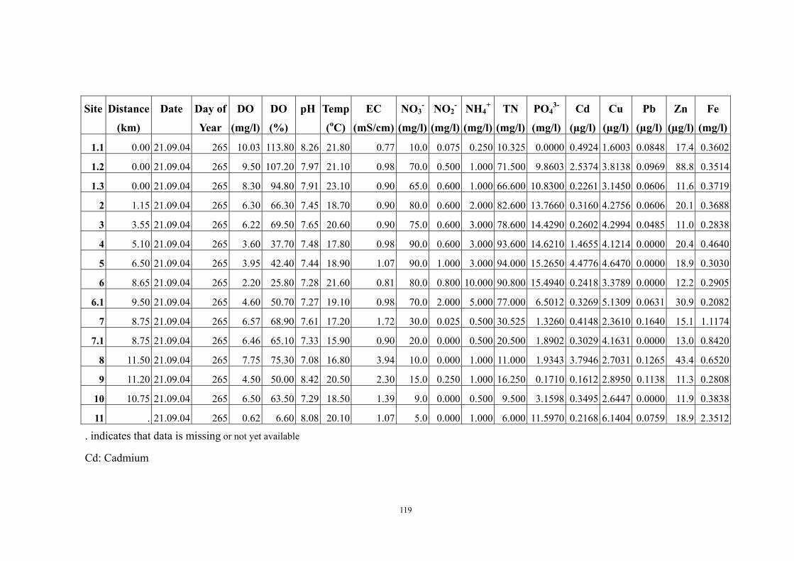
119

Site Distance

(km)

Date Day of

Year

DO

(mg/l)

DO

(%)

pH Temp

(oC)

EC

(mS/cm)

NO3-

(mg/l)

NO2-

(mg/l)

NH4+

(mg/l)

TN

(mg/l)

PO43-

(mg/l)

Cd

(µg/l)

Cu

(µg/l)

Pb

(µg/l)

Zn

(µg/l)

Fe

(mg/l)

1.1 0.00 21.09.04 265 10.03 113.80 8.26 21.80 0.77 10.0 0.075 0.250 10.325 0.0000 0.4924 1.6003 0.0848 17.4 0.3602

1.2 0.00 21.09.04 265 9.50 107.20 7.97 21.10 0.98 70.0 0.500 1.000 71.500 9.8603 2.5374 3.8138 0.0969 88.8 0.3514

1.3 0.00 21.09.04 265 8.30 94.80 7.91 23.10 0.90 65.0 0.600 1.000 66.600 10.8300 0.2261 3.1450 0.0606 11.6 0.3719

2 1.15 21.09.04 265 6.30 66.30 7.45 18.70 0.90 80.0 0.600 2.000 82.600 13.7660 0.3160 4.2756 0.0606 20.1 0.3688

3 3.55 21.09.04 265 6.22 69.50 7.65 20.60 0.90 75.0 0.600 3.000 78.600 14.4290 0.2602 4.2994 0.0485 11.0 0.2838

4 5.10 21.09.04 265 3.60 37.70 7.48 17.80 0.98 90.0 0.600 3.000 93.600 14.6210 1.4655 4.1214 0.0000 20.4 0.4640

5 6.50 21.09.04 265 3.95 42.40 7.44 18.90 1.07 90.0 1.000 3.000 94.000 15.2650 4.4776 4.6470 0.0000 18.9 0.3030

6 8.65 21.09.04 265 2.20 25.80 7.28 21.60 0.81 80.0 0.800 10.000 90.800 15.4940 0.2418 3.3789 0.0000 12.2 0.2905

6.1 9.50 21.09.04 265 4.60 50.70 7.27 19.10 0.98 70.0 2.000 5.000 77.000 6.5012 0.3269 5.1309 0.0631 30.9 0.2082

7 8.75 21.09.04 265 6.57 68.90 7.61 17.20 1.72 30.0 0.025 0.500 30.525 1.3260 0.4148 2.3610 0.1640 15.1 1.1174

7.1 8.75 21.09.04 265 6.46 65.10 7.33 15.90 0.90 20.0 0.000 0.500 20.500 1.8902 0.3029 4.1631 0.0000 13.0 0.8420

8 11.50 21.09.04 265 7.75 75.30 7.08 16.80 3.94 10.0 0.000 1.000 11.000 1.9343 3.7946 2.7031 0.1265 43.4 0.6520

9 11.20 21.09.04 265 4.50 50.00 8.42 20.50 2.30 15.0 0.250 1.000 16.250 0.1710 0.1612 2.8950 0.1138 11.3 0.2808

10 10.75 21.09.04 265 6.50 63.50 7.29 18.50 1.39 9.0 0.000 0.500 9.500 3.1598 0.3495 2.6447 0.0000 11.9 0.3838

11 . 21.09.04 265 0.62 6.60 8.08 20.10 1.07 5.0 0.000 1.000 6.000 11.5970 0.2168 6.1404 0.0759 18.9 2.3512

. indicates that data is missing or not yet available

Cd: Cadmium

120

Cu: Copper

DO: Dissolved oxygen

EC: Electrical conductivity

Fe: Iron

NH4+ : Ammonium ion

NO2- : Nitrite

NO3- : Nitrate

Pb: Lead

PO43- : Phosphate

Temp: Temperature

TN: Total nitrogen

Zn: Zinc