Pattern Recognition 45 (2012) 2432–2444

Contents lists available at SciVerse ScienceDirect

Pattern Recognition

0031-32

doi:10.1

n Corr

Intellige

Spain. T

E-m

journal homepage: www.elsevier.com/locate/pr

A supervised non-linear dimensionality reduction approach formanifold learning

B. Raducanu a, F. Dornaika b,c,n

a Computer Vision Center, Barcelona, Spainb Department of Computer Science and Artificial Intelligence, University of the Basque Country, UPV/EHU, San Sebastian, Spainc IKERBASQUE, Basque Foundation for Science, Bilbao, Spain

a r t i c l e i n f o

Article history:

Received 18 April 2011

Received in revised form

29 November 2011

Accepted 10 December 2011Available online 19 December 2011

Keywords:

Supervised manifold learning

Non-linear dimensionality reduction

Discriminant analysis

Face recognition

03/$ - see front matter & 2011 Elsevier Ltd. A

016/j.patcog.2011.12.006

esponding author at: Department of Com

nce, University of the Basque Country, UPV

el.: þ34 943018034.

ail address: fdornaika@hotmail.fr (F. Dornaika

a b s t r a c t

In this paper we introduce a novel supervised manifold learning technique called Supervised Laplacian

Eigenmaps (S-LE), which makes use of class label information to guide the procedure of non-linear

dimensionality reduction by adopting the large margin concept. The graph Laplacian is split into two

components: within-class graph and between-class graph to better characterize the discriminant

property of the data. Our approach has two important characteristics: (i) it adaptively estimates the

local neighborhood surrounding each sample based on data density and similarity and (ii) the objective

function simultaneously maximizes the local margin between heterogeneous samples and pushes the

homogeneous samples closer to each other.

Our approach has been tested on several challenging face databases and it has been conveniently

compared with other linear and non-linear techniques, demonstrating its superiority. Although we

have concentrated in this paper on the face recognition problem, the proposed approach could also be

applied to other category of objects characterized by large variations in their appearance (such as hand

or body pose, for instance).

& 2011 Elsevier Ltd. All rights reserved.

1. Introduction

In recent years, a new family of non-linear dimensionalityreduction techniques for manifold learning has emerged. Themost known ones are: kernel principal component analysis(KPCA) [1], locally linear embedding (LLE) [2,3], Isomap [4],Supervised Isomap [5], Laplacian Eigenmaps (LE) [6,7]. This familyof non-linear embedding techniques appeared as an alternative totheir linear counterparts which suffer of severe limitation whendealing with real-world data: (i) they assume the data lie in anEuclidean space and (ii) they may fail when the number ofsamples is too small. On the other hand, the non-linear dimen-sionality techniques are able to discover the intrinsic datastructure by exploiting the local topology. In general, theyattempt to optimally preserve the local geometry around eachdata sample while using the rest of the samples to preserve theglobal structure of the data.

In this paper we introduce a novel Supervised LE (S-LE)algorithm, which exploits the class label information for mappingthe original data in the embedded space. The use of labels allows

ll rights reserved.

puter Science and Artificial

/EHU, 20018 San Sebastian,

).

us to split graph Laplacian associated to the data into twocomponents: within-class graph and between-class graph. Ourproposed approach benefits from two important properties: (i) itadaptively estimates the local neighborhood surrounding eachsample based on data density and similarity and (ii) the objectivefunction simultaneously maximizes the local margin betweenheterogeneous samples and pushes the homogeneous samplescloser to each other. The main contributions of our work are asfollows: (1) bypassing the use and selection of a predefinedneighborhood for graph construction and (2) exploiting thediscriminant information in order to get the non-linear embed-ding (spectral projection).

The combination between locality preserving property (inher-ited from the classical LE1) and the discriminative property (dueto the large margin concept) represents a clear advantage for S-LE,compared with other non-linear embedding techniques, becauseit finds a mapping which maximizes the distances between datasamples from different classes at each local area. In other words,it maps the points in an embedded space where data with similarlabels fall close to each other and where the data from differentclasses fall far apart.

The adaptive selection of neighbors for the two graphs repre-sents also an added value to our algorithm. It is well known that a

1 By classical Laplacian Eigenmaps we refer to the algorithm introduced in [6].

B. Raducanu, F. Dornaika / Pattern Recognition 45 (2012) 2432–2444 2433

sensitive matter affecting non-linear embedding techniques isrepresented by the proper choice for neighborhood size. Setting atoo high value for this parameter would result in a loss of localinformation, meanwhile a too low value could result in an over-fragmentation of the manifold (problem known as ‘short-circuit-ing’). For this reason, setting an adequate value for this parameteris crucial in order to confer the approach topological stability.

The rest of the paper is organized as follows. Section 2 reviewssome related work on linear and non-linear dimensionalityreduction techniques. In this section, we also recall, for the sakeof completeness, the classic Laplacian Eigenmaps algorithm.Section 3 is devoted to the presentation of our new proposedalgorithm. Section 4 presents extensive experimental resultsobtained on a man-made object data set and on six face data-bases. Finally, Section 5 contains our conclusions and guidelinesfor future work.

2. Related work

During the last few years, a large number of approaches havebeen proposed for constructing and computing an embeddedsubspace by finding an explicit or non-explicit mapping thatprojects the original data to a new space of lower dimensionality[8–10]. These methods can be grouped into two families: linearand non-linear approaches.

2.1. Linear approaches

The classical linear embedding methods (e.g., PCA, LDA, MDS,maximum margin criterion (MMC) [11]) and locally LDA [12] aredemonstrated to be computationally efficient and suitable forpractical applications, such as pattern classification and visualrecognition. Recent proposed methods attempt to linearize somenon-linear embedding techniques. This linearization is obtainedby forcing the mapping to be explicit, i.e., performing the map-ping by a projection matrix. For example, locality preservingprojection (LPP) [13–15] and neighborhood preserving embed-ding (NPE) [16] can be seen as linearized versions of LE and LLE,respectively. The main advantage of the linearized embeddingtechniques is that the mapping is defined everywhere in theoriginal space. However, since the embedding is approximated bya linear process, these methods ignore the geodesic structure ofthe true manifold. All these linear methods cannot reveal theperfect geometric structure of the non-linear manifold. Someresearchers tried to remedy to the global nature of the linearmethods PCA, LDA and LPP by proposing localized models [17]. Inthis work, localized PCA, LDA, or LPP models are built using theneighbors of a query sample. The authors have shown that theobtained localized linear models can outperform the globalmodels for face recognition and coarse head pose problems.However, it is not clear how neighbors can be optimally selected.In [18], the authors have extended the LPP to the supervised caseby adapting the entries of the similarity matrix according to thelabels of the sample pair. In [19], the authors assessed theperformance of the quotient and difference criteria used in LDA.They also proposed a unified criterion that combines quotient-LDA and difference-LDA criteria.

In addition to the above methods, some distance metriclearning algorithms [20,21] attempt to directly estimate aninduced Mahalanobis distance over the samples. In essence, thesemethods provide a linear transform since the Euclidean distancein the embedded space is equal to the Mahalanobis distance inthe original space. The proposed solutions for estimating theMahalanobis matrix are not given in closed form but by iterativeprocesses.

One interesting supervised linear method is given by [22]. Thiswork proposed a linear discriminant method called averageneighborhood margin maximization (ANMM). Since it estimatesthe linear transform, it can be solved in closed-form instead of theiterative methods. It associates to every sample a margin that isset to the difference between the average distance to hetero-geneous neighbors and the average distance to the homogeneousneighbors. The linear transform is then derived by maximizingthe sum of the margins in the embedded space. A similar methodbased on similar and dissimilar samples was proposed in [23].

2.2. Non-linear approaches

The non-linear methods such as locally linear embedding(LLE), Laplacian Eigenmaps, Isomap, Hessian LLE (hLLE) [24] focuson preserving the local structure of data. LLE formulates themanifold learning problem as a neighborhood-preserving embed-ding, which learns the global structure by exploiting the localsymmetries of linear reconstructions. Isomap extends the classi-cal multidimensional scaling (MDS) [25] by computing the pair-wise distances in the geodesic space of the manifold. Essentially,Isomap attempts to preserve geodesic distances when data areembedded in the new low dimensional space. Based on thespectral decomposition of the graph Laplacian, Laplacian Eigen-maps actually try to find Laplacian eigenfunction on the manifold.Maximum variance unfolding (MVU) [26] is a global algorithm fornon-linear dimensionality reduction, in which all the data pairs,nearby and far, are considered. MVU attempts to ‘unfold’ a dataset by pulling the input patterns as far apart as possible subject tothe constraints that distances and angles between neighboringpoints are strictly preserved.

The non-linear embedding methods have been successfullyapplied to some standard data sets and generated satisfyingresults in dimensionality reduction and manifold visualization.However, most of these approaches does not take into account thediscriminant information that is usually available for many realworld problems. Therefore, the application of these methods canbe very satisfactory in terms of dimensionality reduction andvisualization but can be fair for classification tasks. In [5], theauthors propose a supervised version of Isomap. This versionreplaces pairwise Euclidean distances by a dissimilarity functionthat increases if the pair is heterogeneous and decreases other-wise. Since this algorithm is inherited from Isomap it suffers fromthe same disadvantage in the sense that outlier samples can giverise to an unwanted embedded space. In [27], the authors exploitlabel information to improve Laplacian Eigenmaps. The proposedmethod affects the computation of the affinity matrix entries inthe sense that a homogeneous pair of neighbors will have largevalue and heterogeneous pairs of neighbors will have a smallvalue. Although, the authors show some performance improve-ment, the proposed method has two drawbacks. First, there is noguarantee that the heterogeneous samples will be pushed awayfrom each other. Second, the method has at least three para-meters to be tuned.

Some works extended the locally linear embedding (LLE)technique to the supervised case [28,29]. These extensions weremade in the first stage of the LLE algorithm, i.e., the neighborhoodgraph construction. In these works, the K nearest neighbors of agiven sample are looked for among the samples belonging to thesame class.

As can be seen, all existing supervised non-linear dimension-ality reduction techniques have used the labels either for adjust-ing the entries of a similarity matrix or for modifying theneighborhood graph. However, our proposed method exploitsthe large margin concept in order to increase the discriminationbetween homogeneous and heterogeneous samples.

B. Raducanu, F. Dornaika / Pattern Recognition 45 (2012) 2432–24442434

2.2.1. Review of Laplacian Eigenmaps

To make the paper self-contained, this section will brieflypresent the Laplacian Eigenmaps (LE). Throughout the paper,capital bold letters denote matrices and small bold letters denotevectors.

Laplacian Eigenmaps is a recent non-linear dimensionalityreduction techniques that aims to preserve the local structure ofdata [6]. Using the notion of the Laplacian of the graph, this non-supervised algorithm computes a low-dimensional representationof the data set by optimally preserving local neighborhoodinformation in a certain sense. We assume that we have a set ofN samples fyig

Ni ¼ 1 �RD. Let’s define a neighborhood graph on

these samples, such as a K-nearest-neighbor or E-ball graph, or afull mesh, and weigh each edge yi � yj by a symmetric affinityfunction Wij ¼ Kðyi; yjÞ, typically Gaussian:

Wij ¼ exp �Jyi�yjJ

2

b

!ð1Þ

where b is usually set to the average of squared distancesbetween all pairs.

We seek latent points fxigNi ¼ 1 �RL that minimize 1

2

Pi,j

Jxi�xjJ2Wij, which discourages placing far apart latent points

that correspond to similar observed points. If W�Wij denotes thesymmetric affinity matrix and D is the diagonal weight matrix,whose entries are column (or row, since W is symmetric) sums ofW, then the Laplacian matrix is given by L¼D�W. It can beshown that the objective function can also be written as (Asimilar derivation is given in Section 3.3.):

1

2

Xi,j

Jxi�xjJ2Wij ¼ trðZT LZÞ ð2Þ

where Z¼ ½xT1; . . . ;x

TN� is the N� L embedding matrix and trð�Þ

denotes the trace of a matrix. The ith row of the matrix Z providesthe vector xi—the embedding coordinates of the sample yi.

The embedding matrix Z is the solution of the optimizationproblem:

minZ

trðZT LZÞ s:t: ZT DZ¼ I, ZT Le¼ 0 ð3Þ

where I is the identity matrix and e¼ ð1, . . . ,1ÞT . The firstconstraint eliminates the trivial solution Z¼ 0 (by setting anarbitrary scale) and the second constraint eliminates the trivialsolution e (all samples are mapped to the same point). Standardmethods show that the embedding matrix is provided by thematrix of eigenvectors corresponding to the smallest eigenvaluesof the generalized eigenvector problem,

Lz¼ lDz ð4Þ

Let the column vectors z0, . . . ,zN�1 be the solutions of (4), orderedaccording to their eigenvalues, l0 ¼ 0rl1r � � �rlN�1. Theeigenvector corresponding to eigenvalue 0 is left out and onlythe next eigenvectors for embedding are used. The embedding ofthe original samples is given by the row vectors of the matrix Z,that is,

yi�!xi ¼ ðz1ðiÞ, . . . ,zLðiÞÞT

ð5Þ

where LoN is the dimension of the new space. From Eq. (4), wecan observe that the dimensionality of the subspace obtained byLE is limited by the number of samples N.

3. Supervised Laplacian Eigenmaps

While the LE may give good results for non-linear dimension-ality reduction, it has not been widely used and assessed forclassification tasks. Indeed, many experiments show that the

recognition rate in the embedded space can be highly dependingon the choice of the neighborhood size in the reconstructed graph[15,30,31]. Choosing the ideal size, K or E, in advance can be a verydifficult task. Moreover, the introduced mapping by LE does notexploit the discriminant information given by the labels of data.In this section, we present our Supervised LE algorithm which hastwo interesting properties: (i) it adaptively estimates the localneighborhood surrounding each sample based on data densityand similarity and (ii) the objective function simultaneouslymaximizes the local margin between heterogeneous samplesand pushes the homogeneous samples closer to each other. Wewould like to remind that the main contributions of our approachare: (1) bypassing the use and selection of a predefined neighbor-hood for graph construction and (2) exploiting the discriminantinformation in order to get the non-linear embedding (spectralprojection).

3.1. Two graphs and adaptive neighborhood

In order to discover both geometrical and discriminant struc-ture of the data manifold, we split the global graph into twocomponents: the within-class graph Gw and between-class graphGb. Let lðyiÞ be the class label of yi. For each data point yi, wecompute two subsets, NbðyiÞ and NwðyiÞ. NwðyiÞ contains theneighbors sharing the same label with yi, while NbðyiÞ containsthe neighbors having different labels. We stress the fact thatunlike the classical LE, our algorithm adapts the size of both setsaccording to the local sample point yi and its similarities with therest of samples. To this end, each set is defined for each samplepoint yi and is computed in two consecutive steps. First, theaverage similarity of the sample yi is computed by the total of allsimilarities with the rest of the data set (Eq. (6)). Second, the setsNwðyiÞ and NbðyiÞ are computed using Eqs. (7) and (8), respec-tively:

ASðyiÞ ¼1

N

XN

k ¼ 1

exp �Jyi�ykJ

2

b

!ð6Þ

NwðyiÞ ¼ yj9lðyjÞ ¼ lðyiÞ,exp �Jyi�yjJ

2

b

!4ASðyiÞ

( )ð7Þ

NbðyiÞ ¼ yj9lðyjÞa lðyiÞ,exp �Jyi�yjJ

2

b

!4ASðyiÞ

( )ð8Þ

Eq. (7) means that the set of within-class neighbors of thesample yi, NwðyiÞ, is all data samples that have the same label of yi

and that have a similarity higher than the average similarityassociated with yi. There is a similar interpretation for the set ofbetween-class neighbors NbðyiÞ. From Eqs. (7) and (8) it is clearthat the neighborhood size is not the same for every data sample.This mechanism adapts the set of neighbors according to the localdensity and similarity between data samples in the original space.It is worth noting that for real data sets the mean similarity isalways a positive value.

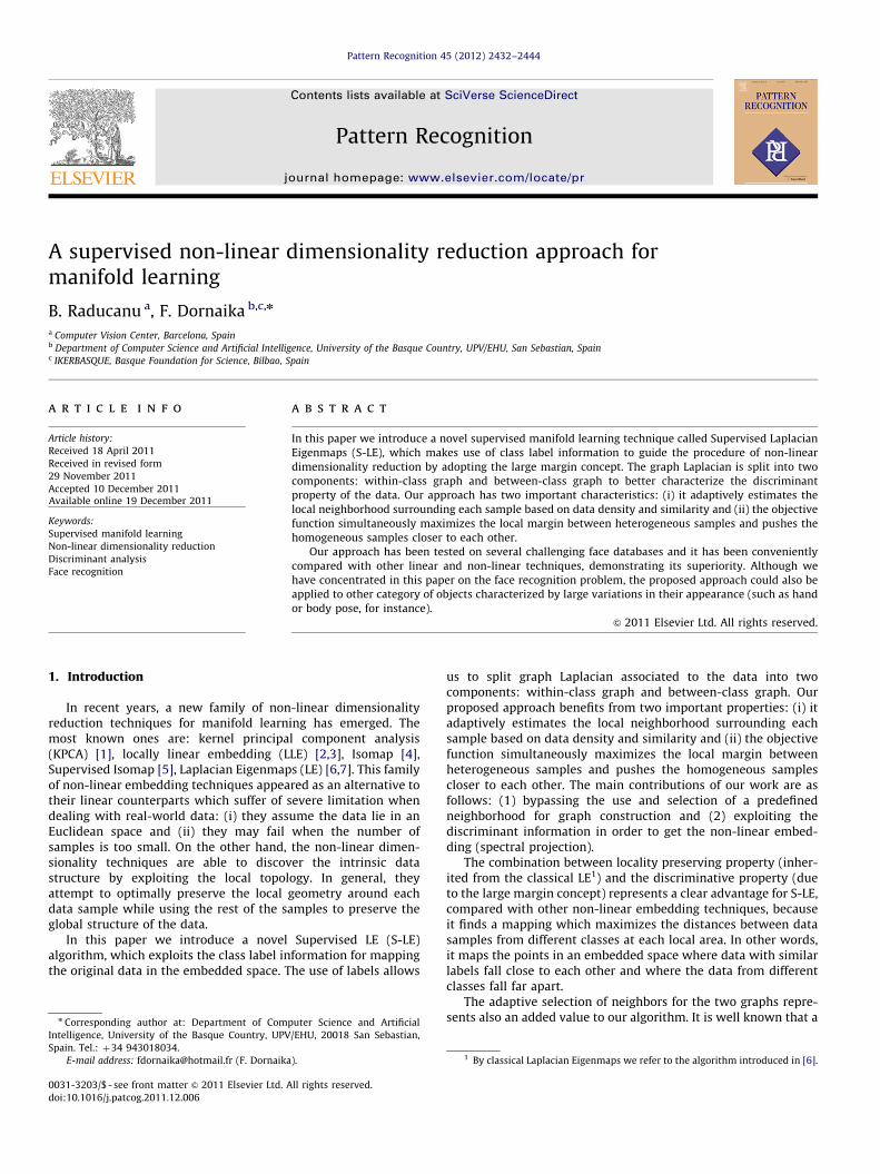
It is obvious that Eqs. (6)–(8) computes a sample-based neighbor-hood for every sample. A simple geometrical interpretation of theseequations is illustrated in Fig. 1. In Fig. 1(a), the average similarity ofthe sample P1 is relatively low. Thus, according to Eqs. (7) and (8), theneighborhood of the sample P1 will be relatively large, i.e., the sampleP1 will have many neighbors (both homogeneous and heteroge-neous). In Fig. 1(b), the average similarity of the sample P1 is relativelyhigh so its neighborhood will be small. From the above equations, onecan conclude that an isolated sample will have a small meansimilarity which increases the chance that other samples will con-sider it as a graph neighbor. This is less likely to happen with a fixedneighborhood size where the edges of the graph will be kept within

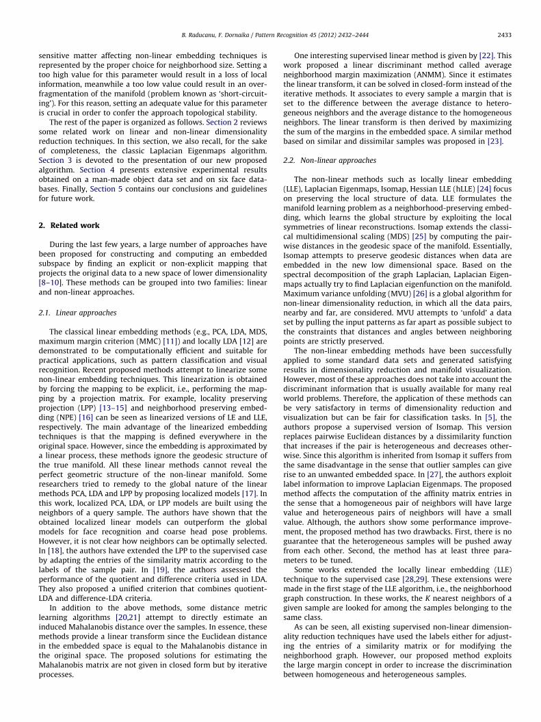
Fig. 2. (a) Before embedding: In the original space, the sample P1 has three

neighbors. The samples with the same color and shape belong to the same class.

The first row of the within class similarity matrix Ww and of the between class

similarity matrix Wb . (b) After embedding: the non-linear embedding obtained by

the proposed S-LE. (For interpretation of the references to color in this figure

legend, the reader is referred to the web version of this article.)Fig. 1. Sample-based neighbor computation exploits a sample-based measure

which relates the sample to the whole set of data. (a) The average similarity of P1

is relatively low so the neighborhood of P1 will be extended. (b) The average

similarity of P1 is relatively high so its neighborhood will be somehow small.

B. Raducanu, F. Dornaika / Pattern Recognition 45 (2012) 2432–2444 2435

the dense regions. Since the concepts of similarity and closeness ofsamples are tightly related, one can conclude, at first glance, that ourintroduced strategy for adaptive estimation of neighbors is equivalentto the use of an e-ball neighborhood. It is worth noting that there aretwo main differences: (1) the use of an e-ball neighborhood requires auser-defined value for the ball radius e and (2) the ball radius isconstant for all data samples, whereas our strategy uses an adaptivethreshold (Eq. (6)) that depends on the local sample. Thus, ourstrategy adapts the graph construction to all databases withoutparameter tuning.

3.2. Two affinity matrices

Let Ww and Wb be the weight matrices of Gw and Gb,respectively. These matrices are defined as

Ww,ij ¼exp �

Jyi�yjJ2

b

!if yjANwðyiÞ or yiANwðyjÞ

0 otherwise

8><>:

Wb,ij ¼1 if yjANbðyiÞ or yiANbðyjÞ

0 otherwise

�

If the same type of weighting is used (0–1 weighting or Gaussiankernel weighting), then it is easy to show that the global affinitymatrix, W, associated with the Laplacian Eigenmaps graph can be

written as

W¼WwþWb

Fig. 2 illustrates the principle of the proposed S-LE. It alsoshows how the graph weight matrices are computed using thesample-based neighborhood.

3.3. Optimal mapping

Each data sample yi is mapped into a vector xi. The aim is tocompute the embedded coordinates xi for each data sample. Theobjective functions are

min1

2

Xi,j

Jxi�xjJ2Ww,ij ð9Þ

max1

2

Xi,j

Jxi�xjJ2Wb,ij ð10Þ

Let the matrix Z denotes ½xT1; . . . ;x

TN �, it can be shown that the

above objective functions can be written as

min trðZT LwZÞ ð11Þ

max trðZT LbZÞ ð12Þ

where Lw ¼Dw�Ww and Lb ¼Db�Wb.Using the scale constraint ZT DwZ¼ I and the equation

Lw ¼Dw�Ww, the above two objective functions can be combined

B. Raducanu, F. Dornaika / Pattern Recognition 45 (2012) 2432–24442436

into one single objective function:

arg maxZfg trðZT LbZÞþð1�gÞtrðZT WwZÞg s:t: ZT DwZ¼ I

where g is a real scalar that belongs to [0,1]. By using the matrixB¼ gLbþð1�gÞWw, the problem becomes

arg maxZ

trðZT BZÞ s:t: ZT DwZ¼ I

This gives a generalized eigenvalue problem having the fol-lowing form:

Bz¼ lDwz ð13Þ

Let the column vectors z1,z2, . . . ,zL be the generalized eigen-vectors of (13) according to their eigenvalue: l1Zl2Z � � �ZlL.Then, the N� L embedding matrix Z¼ ½xT

1; . . . ;xTN� will be given by

concatenating the obtained eigenvectors Z¼ ½z1,z2, . . . ,zL�.It is worth noting that the outlier labels have no significant

impact on the learned embedding since the method relies onpenalizing local geometric distances in the mapped space. Indeed,Eq. (6) does not depend on the labels and thus it is invariant to theoutlier labels. Regarding Eqs. (7) and (8) and assuming that amislabeled sample is within the selected neighborhood, then themechanism of pushing and pulling will be reversed for only thissample, while the rest of all samples will contribute to the correctdesired behavior.

3.4. Theoretical analysis of the proposed approach

3.4.1. Difference between the classic LE and the proposed S-LE

The main differences between the classic LE and our proposedS-LE are as follows:

The classic LE has one single objective, namely preserving thelocality of samples. The proposed S-LE aims at a discriminantanalysis via a non-linear embedding. The classic LE does notexploit the sample labels. This means that the only objective ofthe classic LE is to preserve locality of samples. On the otherhand, our proposed S-LE exploits the labels of samples by col-lapsing homogeneous neighbors, and pulling away heteroge-neous neighbors. In other words, the constructed graph is splitinto two graphs: within class graph and between class graph.

2 http://www.cs.columbia.edu/CAVE/software/softlib/coil-20.php3 http://www.cl.cam.ac.uk/research/dtg/attarchive/facedatabase.html4 http://www.shef.ac.uk/eee/research/vie/research/face.html5 http://see.xidian.edu.cn/vipsl/database_Face.html6 http://vision.ucsd.edu/� leekc/ExtYaleDatabase/ExtYaleB.html

The classic LE works on a single graph that is built using anartificial graph. The most popular graph construction manneris based on the K nearest neighbor and E-ball neighborhoodcriteria. K and E are user-defined parameters that should befixed in advance. It is well known that the choice of theseparameters can affect the performance of the embedding. Onthe other hand, our graph does not need a user-definedparameter. Instead, the graph edges are set according toadaptive neighborhood that is only sample-based. Therefore,our proposed strategy for graph construction can automati-cally adapt the graph to all databases without parameteradjustment. Thus, looking for the best value for either K or Eis bypassed by the proposed approach.

3.4.2. Relation to normalized graph-cut formulation

There is some similarity between the use of the Laplacianformulations and normalized cut formulations [32,33]. However,we stress the fact that there are two main differences betweenour proposed formulation and the normalized cut formulation.Indeed, the objectives and the Laplacian computation are differ-ent. (i) Our introduced method is fully supervised and addressesclassification tasks. On the other hand, the normalized cutformulations address the clustering problems from unlabeledsamples—it can be unsupervised or semi-supervised technique.

(ii) Our proposed method computes two Laplacian matrices basedon local similarity and labels, whereas in the Normalized cutformulation, the computation of the Laplacian matrix relies on theconcept of similarity among unlabeled samples.

4. Experimental results

In this section, we report the experimental results obtainedfrom the application of our proposed algorithm to the problem ofvisual pattern recognition. Extensive experiments in terms ofclassification accuracy have been carried out on a man-madeobject database as well as on some public face databases. All thesedatabases are characterized by a large variation in objectappearance.

4.1. COIL-20 database

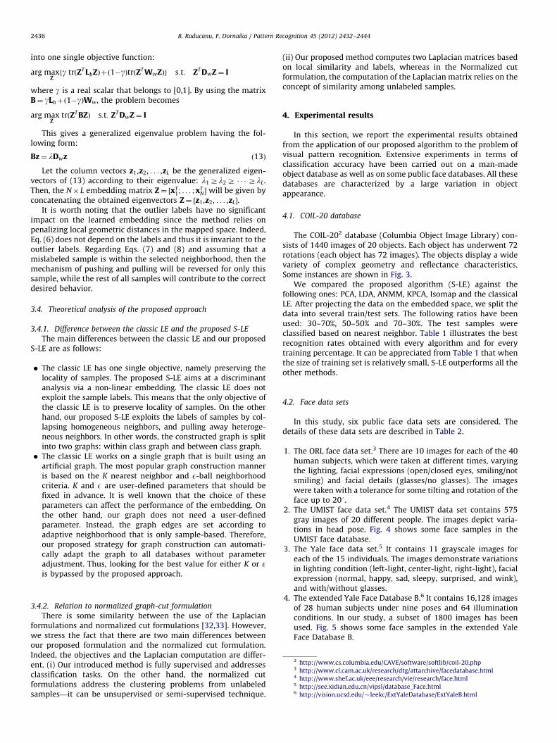
The COIL-202 database (Columbia Object Image Library) con-sists of 1440 images of 20 objects. Each object has underwent 72rotations (each object has 72 images). The objects display a widevariety of complex geometry and reflectance characteristics.Some instances are shown in Fig. 3.

We compared the proposed algorithm (S-LE) against thefollowing ones: PCA, LDA, ANMM, KPCA, Isomap and the classicalLE. After projecting the data on the embedded space, we split thedata into several train/test sets. The following ratios have beenused: 30–70%, 50–50% and 70–30%. The test samples wereclassified based on nearest neighbor. Table 1 illustrates the bestrecognition rates obtained with every algorithm and for everytraining percentage. It can be appreciated from Table 1 that whenthe size of training set is relatively small, S-LE outperforms all theother methods.

4.2. Face data sets

In this study, six public face data sets are considered. Thedetails of these data sets are described in Table 2.

1.

The ORL face data set.3 There are 10 images for each of the 40human subjects, which were taken at different times, varyingthe lighting, facial expressions (open/closed eyes, smiling/notsmiling) and facial details (glasses/no glasses). The imageswere taken with a tolerance for some tilting and rotation of theface up to 201.

2.

The UMIST face data set.4 The UMIST data set contains 575gray images of 20 different people. The images depict varia-tions in head pose. Fig. 4 shows some face samples in theUMIST face database.

3.

The Yale face data set.5 It contains 11 grayscale images foreach of the 15 individuals. The images demonstrate variationsin lighting condition (left-light, center-light, right-light), facialexpression (normal, happy, sad, sleepy, surprised, and wink),and with/without glasses.

4.

The extended Yale Face Database B.6 It contains 16,128 imagesof 28 human subjects under nine poses and 64 illuminationconditions. In our study, a subset of 1800 images has beenused. Fig. 5 shows some face samples in the extended YaleFace Database B.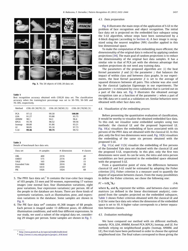

Fig. 3. The 20 objects of COIL-20 data set.

Table 1Best recognition accuracy obtained with COIL20 data set. The classification

accuracy when the training/test percentage was set to 30–70%, 50–50% and

70–30%, respectively.

Method COIL-20 (30/70) (%) COIL-20 (50/50) (%) COIL-20 (70/30) (%)

PCA 97.12 99.30 100.00LDA 91.27 93.88 93.75

ANMM 90.1 94.3 96.4

KPCA 95.78 98.52 99.56

Isomap 88.80 91.86 93.21

LE 90.05 95.18 97.73

S-LE 99.46 99.75 99.72

Table 2Details of benchmark face data sets.

Data set # samples # dimension # classes

ORL 400 2576 40

UMIST 575 2576 20

YALE 165 2304 15

Extended Yale 1800 2016 28

PF01 1819 2304 107

PIE 1926 1024 68

B. Raducanu, F. Dornaika / Pattern Recognition 45 (2012) 2432–2444 2437

5.

The PF01 face data set.7 It contains the true-color face imagesof 103 people, 53 men and 50 women, representing 17 variousimages (one normal face, four illumination variations, eightpose variations, four expression variations) per person. All ofthe people in the database are Asians. There are three kinds ofsystematic variations, such as illumination, pose, and expres-sion variations in the database. Some samples are shown inFig. 6.

6.

The PIE face data set8 contains 41,368 images of 68 people.Each person is imaged under 13 different poses, 43 differentillumination conditions, and with four different expressions. Inour study, we used a subset of the original data set, consider-ing 29 images per person. Some samples are shown in Fig. 7.

7 http://nova.postech.ac.kr/special/imdb/imdb.html8 http://www.ri.cmu.edu/projects/project_418.html

4.3. Data preparation

Fig. 8 illustrates the main steps of the application of S-LE to theproblem of face recognition and object recognition. The initialface data set is projected on the embedded face subspace usingthe S-LE algorithm, whose steps have been summarized by a4-block diagram (according to Section 4). A face image is recog-nized using the nearest neighbor (NN) classifier applied in thislow dimensional space.

To make the computation of the embedding more efficient, thedimensionality of the original data is reduced by applying randomprojections [34]. The main goal of random projections is to reducethe dimensionality of the original face data samples. It has asimilar role to that of PCA yet with the obvious advantage thatrandom projections do not need any training data.

The parameters of the proposed algorithm are: (i) the heatKernel parameter b and (ii) the parameter g that balances theimpact of within class and between class graphs. In our experi-ments, the heat Kernel parameter b is set to the average ofsquared distances between all pairs. This scheme was also usedby the classical Laplacian Eigenmaps in our experiments. Theparameter g is estimated by cross-validation that is carried out ona part of the data set. Fig. 9 illustrates the obtained averagerecognition rate as a function of the parameter g when a part ofthe ORL data set is used as a validation set. Similar behaviors wereobtained with other face data sets.

4.4. Visualization of the embedding process

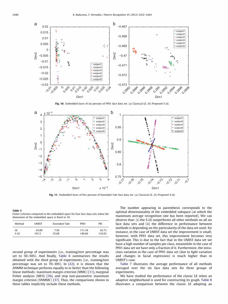
Before presenting the quantitative evaluation of classification,it would be worthy to visualize the obtained embedded face data.To this end, we visualize some embedded samples using twomethods: the classical LE and the proposed Supervised LE.Fig. 10(a) visualizes the embedding of faces associated with sixpersons of the PF01 data set obtained with the classical LE. In thisplot, only the first two dimensions were used. Fig. 10(b) visualizesthe embedding of the same six persons obtained with theproposed S-LE.

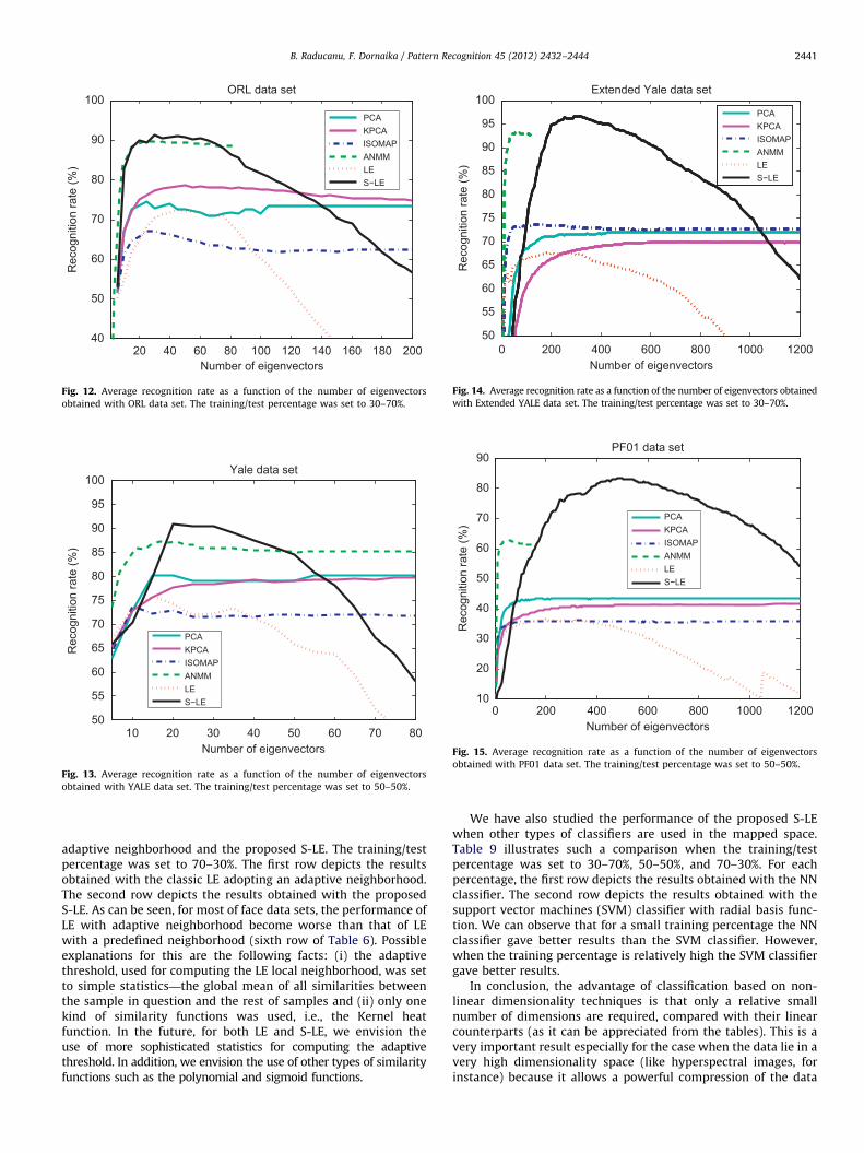
Fig. 11(a) and 11(b) visualize the embedding of five personsof the Extended Yale data set obtained with the classical LE andthe proposed S-LE, respectively. In this plot, only the first twodimensions were used. As can be seen, the intra and extra personvariabilities are best presented in the embedded space obtainedwith the proposed S-LE.

From a quantitative point of view, the differences betweenclassical LE and S-LE could be estimated by adopting the Fishercriterion [35]. Fisher criterion is a measure used to quantify thedegree of separation between classes. From the many possibilitiesto define the Fisher criterion, we chose the following one:

FC ¼ trðS�1w SbÞ ð14Þ

where Sw and Sb represent the within- and between-class scattermatrices (as defined in the linear discriminant analysis), com-puted from the samples projected on the embedded subspaces.Table 3 shows Fisher criterion obtained with the classical LE andS-LE for some face data sets when the dimension of the embeddedspace is set to 10. A higher value corresponds to a better separa-tion between classes.

4.5. Evaluation methodology

We have compared our method with six different methods,namely: PCA, LDA, ANMM, Kernel PCA (KPCA), Isomap, and LE. Formethods relying on neighborhood graphs (Isomap, ANMM, andLE), five trials have been performed in order to choose the optimalneighborhood size. The final values correspond to those giving the

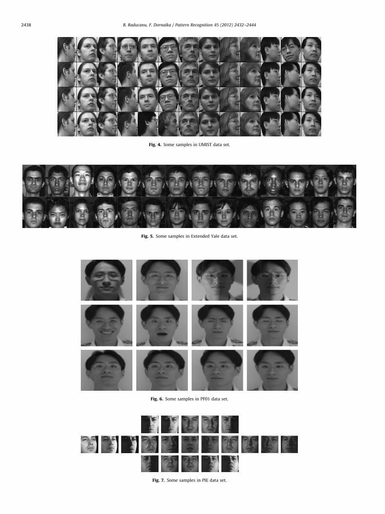
Fig. 5. Some samples in Extended Yale data set.

Fig. 6. Some samples in PF01 data set.

Fig. 7. Some samples in PIE data set.

Fig. 4. Some samples in UMIST data set.

B. Raducanu, F. Dornaika / Pattern Recognition 45 (2012) 2432–24442438

Fig. 8. Supervised Laplacian Eigenmaps embedding for the face recognition problem.

0.1 0.2 0.3 0.4 0.5 0.6 0.7 0.8 0.978

80

82

84

86

88

90

92

94

96

98

γ

Rec

ogni

tion

rate

(%)

Fig. 9. Average recognition rate as a function of the blending parameter g using a

part of the ORL data set.

9 This dimension is bounded by the dimension of the input samples.

B. Raducanu, F. Dornaika / Pattern Recognition 45 (2012) 2432–2444 2439

best recognition rate in test sets. The implementation of themethods PCA, LDA, KPCA, and Isomap were retrieved from http://www.zjucadcg.cn/dengcai/Data/data.html. We have implementedthe ANMM method and the classic LE.

For each face data set and for every method, we conductedthree groups of experiments for which the percentage of trainingsamples was set to 30%, 50% and 70% of the whole data set. Theremaining data was used for testing. The partition of the data setwas done randomly.

For a given embedding method, the recognition rate wascomputed for several dimensions belonging to ½1,Lmax�. For mostof the tested methods Lmax is equal to the number of samples usedexcept for LDA and ANMM. For LDA, the maximum dimension isequal to the number of classes minus one. For ANMM themaximum dimension is variable since it is equal to the numberof positive eigenvalues.9

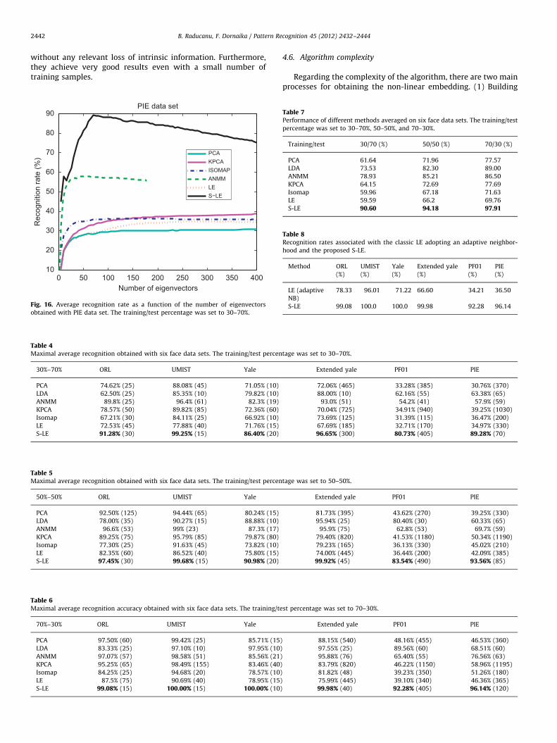
Figs. 12, 13, 14, 15, and 16 illustrate the average recognitionrate associated with ORL, Yale, Extended Yale, PF01, and PIE datasets, respectively. The average recognition rate was computed(over 10 folds) by PCA, KPCA, Isomap, ANMM, LE, and S-LE. Thetraining/test percentage was set to 50–50% for YALE and PF01data sets, and to 30–70% for ORL, Extended Yale, and PIE data sets.Since the maximum dimension for LDA is equal to the number ofclasses minus one, the corresponding curve was not plotted. Itsrate was reported in Tables 4–6. The maximum dimensiondepicted in the plots was set to a fraction of Lmax, in order toguarantee meaningful results. Moreover, we can observe thatafter a given dimension the recognition rate associated with thethree methods PCA, KPCA, and Isomap becomes stable. However,the recognition rate associated with LE and S-LE methodsdecreases if the number of used eigenvectors becomes large—ageneral trend associated with many non-linear methods. Thismeans that the last eigenvectors do not have any discriminantinformation, lacking completely of statistical significance.

The best (average) performance obtained by the embeddingalgorithms, based on 10 random splits, are shown in Tables 4–6,respectively. Table 4 summarizes the results obtained with thefirst group of experiments (i.e., training/test percentage was set to30–70%). Table 5 summarizes the results obtained with the

−0.01

−0.00

5 00.0

05 0.010.0

15 0.02

0.025 0.0

30.0

35 0.04

−0.03

−0.025

−0.02

−0.015

−0.01

−0.005

0

0.005

0.01

0.015

0.02

Dim1

Dim

2

subject1subject2subject3subject4subject5subject6

0.288

2

0.288

4

0.288

6

0.288

80.2

89

0.289

2

0.289

4

0.289

6

0.289

8−0.473

−0.472

−0.471

−0.47

−0.469

−0.468

−0.467

Dim1

Dim

2

subject1subject2subject3subject4subject5subject6

Fig. 10. Embedded faces of six persons of PF01 face data set. (a) Classical LE. (b) Proposed S-LE.

−4 −3 −2 −1 0 1 2 3 4−5

−4

−3

−2

−1

0

1

2

3

4 x 10−3

x 10−3Dim1

Dim

2

subject1subject2subject3subject4subject5

−0.77

−0.76

−0.75

−0.74

−0.73

−0.72

−0.71 −0

.70.75

0.8

0.85

0.9

0.95

1

Dim1

Dim

2

subject1subject2subject3subject4subject5

Fig. 11. Embedded faces of five persons of Extended Yale face data set. (a) Classical LE. (b) Proposed S-LE.

Table 3Fisher criterion computed in the embedded space for four face data sets when the

dimension of the embedded space is fixed to 10.

Method UMIST Extended Yale PF01 PIE

LE 43.00 7.56 111.34 42.73

S-LE 101.5 25.68 140.66 116.92

B. Raducanu, F. Dornaika / Pattern Recognition 45 (2012) 2432–24442440

second group of experiments (i.e., training/test percentage wasset to 50–50%). And finally, Table 6 summarizes the resultsobtained with the third group of experiments (i.e., training/testpercentage was set to 70–30%). In [22], it is shown that theANMM technique performs equally to or better than the followinglinear methods: maximum margin criterion (MMC) [11], marginalFisher analysis (MFA) [36], and step non-parametric maximummargin criterion (SNMMC) [37]. Thus, the comparisons shown inthese tables implicitly include these methods.

The number appearing in parenthesis corresponds to theoptimal dimensionality of the embedded subspace (at which themaximum average recognition rate has been reported). We canobserve that: (i) the S-LE outperforms all other methods on all sixface data sets and (ii) the difference in performance betweenmethods is depending on the particularity of the data set used: forinstance, in the case of UMIST data set the improvement is small;however, with PF01 data set, this improvement becomes verysignificant. This is due to the fact that in the UMIST data set wehave a high number of samples per class, meanwhile in the case ofPF01 data set we have only a fraction of it. Furthermore, the intra-class variation in the case of PF01 data set (due to light variationand changes in facial expression) is much higher than inUMIST’s case.

Table 7 illustrates the average performance of all methodsaveraged over the six face data sets for three groups ofexperiments.

We have studied the performance of the classic LE when anadaptive neighborhood is used for constructing its graph. Table 8illustrates a comparison between the classic LE adopting an

20 40 60 80 100 120 140 160 180 20040

50

60

70

80

90

100

Number of eigenvectors

Rec

ogni

tion

rate

(%)

ORL data set

PCAKPCAISOMAPANMMLES−LE

Fig. 12. Average recognition rate as a function of the number of eigenvectors

obtained with ORL data set. The training/test percentage was set to 30–70%.

10 20 30 40 50 60 70 8050

55

60

65

70

75

80

85

90

95

100

Number of eigenvectors

Rec

ogni

tion

rate

(%)

Yale data set

PCAKPCAISOMAPANMMLES−LE

Fig. 13. Average recognition rate as a function of the number of eigenvectors

obtained with YALE data set. The training/test percentage was set to 50–50%.

0 200 400 600 800 1000 120050

55

60

65

70

75

80

85

90

95

100

Number of eigenvectors

Rec

ogni

tion

rate

(%)

Extended Yale data set

PCAKPCAISOMAPANMMLES−LE

Fig. 14. Average recognition rate as a function of the number of eigenvectors obtained

with Extended YALE data set. The training/test percentage was set to 30–70%.

0 200 400 600 800 1000 120010

20

30

40

50

60

70

80

90

Number of eigenvectors

Rec

ogni

tion

rate

(%)

PF01 data set

PCAKPCAISOMAPANMMLES−LE

Fig. 15. Average recognition rate as a function of the number of eigenvectors

obtained with PF01 data set. The training/test percentage was set to 50–50%.

B. Raducanu, F. Dornaika / Pattern Recognition 45 (2012) 2432–2444 2441

adaptive neighborhood and the proposed S-LE. The training/testpercentage was set to 70–30%. The first row depicts the resultsobtained with the classic LE adopting an adaptive neighborhood.The second row depicts the results obtained with the proposedS-LE. As can be seen, for most of face data sets, the performance ofLE with adaptive neighborhood become worse than that of LEwith a predefined neighborhood (sixth row of Table 6). Possibleexplanations for this are the following facts: (i) the adaptivethreshold, used for computing the LE local neighborhood, was setto simple statistics—the global mean of all similarities betweenthe sample in question and the rest of samples and (ii) only onekind of similarity functions was used, i.e., the Kernel heatfunction. In the future, for both LE and S-LE, we envision theuse of more sophisticated statistics for computing the adaptivethreshold. In addition, we envision the use of other types of similarityfunctions such as the polynomial and sigmoid functions.

We have also studied the performance of the proposed S-LEwhen other types of classifiers are used in the mapped space.Table 9 illustrates such a comparison when the training/testpercentage was set to 30–70%, 50–50%, and 70–30%. For eachpercentage, the first row depicts the results obtained with the NNclassifier. The second row depicts the results obtained with thesupport vector machines (SVM) classifier with radial basis func-tion. We can observe that for a small training percentage the NNclassifier gave better results than the SVM classifier. However,when the training percentage is relatively high the SVM classifiergave better results.

In conclusion, the advantage of classification based on non-linear dimensionality techniques is that only a relative smallnumber of dimensions are required, compared with their linearcounterparts (as it can be appreciated from the tables). This is avery important result especially for the case when the data lie in avery high dimensionality space (like hyperspectral images, forinstance) because it allows a powerful compression of the data

B. Raducanu, F. Dornaika / Pattern Recognition 45 (2012) 2432–24442442

without any relevant loss of intrinsic information. Furthermore,they achieve very good results even with a small number oftraining samples.

0 50 100 150 200 250 300 350 40010

20

30

40

50

60

70

80

90

Number of eigenvectors

Rec

ogni

tion

rate

(%)

PIE data set

PCAKPCAISOMAPANMMLES−LE

Fig. 16. Average recognition rate as a function of the number of eigenvectors

obtained with PIE data set. The training/test percentage was set to 30–70%.

Table 4Maximal average recognition obtained with six face data sets. The training/test percen

30%–70% ORL UMIST Yale

PCA 74.62% (25) 88.08% (45) 71.05% (10)

LDA 62.50% (25) 85.35% (10) 79.82% (10)

ANMM 89.8% (25) 96.4% (61) 82.3% (19)

KPCA 78.57% (50) 89.82% (85) 72.36% (60)

Isomap 67.21% (30) 84.11% (25) 66.92% (10)

LE 72.53% (45) 77.88% (40) 71.76% (15)

S-LE 91.28% (30) 99.25% (15) 86.40% (20)

Table 5Maximal average recognition obtained with six face data sets. The training/test percen

50%–50% ORL UMIST Yale

PCA 92.50% (125) 94.44% (65) 80.24% (15)

LDA 78.00% (35) 90.27% (15) 88.88% (10)

ANMM 96.6% (53) 99% (23) 87.3% (17)

KPCA 89.25% (75) 95.79% (85) 79.87% (80)

Isomap 77.30% (25) 91.63% (45) 73.82% (10)

LE 82.35% (60) 86.52% (40) 75.80% (15)

S-LE 97.45% (30) 99.68% (15) 90.98% (20)

Table 6Maximal average recognition accuracy obtained with six face data sets. The training/te

70%–30% ORL UMIST Yale

PCA 97.50% (60) 99.42% (25) 85.71% (15)

LDA 83.33% (25) 97.10% (10) 97.95% (10)

ANMM 97.07% (57) 98.58% (51) 85.56% (21)

KPCA 95.25% (65) 98.49% (155) 83.46% (40)

Isomap 84.25% (25) 94.68% (20) 78.57% (10)

LE 87.5% (75) 90.69% (40) 78.95% (15)

S-LE 99.08% (15) 100.00% (15) 100.00% (10)

4.6. Algorithm complexity

Regarding the complexity of the algorithm, there are two mainprocesses for obtaining the non-linear embedding. (1) Building

tage was set to 30–70%.

Extended yale PF01 PIE

72.06% (465) 33.28% (385) 30.76% (370)

88.00% (10) 62.16% (55) 63.38% (65)

93.0% (51) 54.2% (41) 57.9% (59)

70.04% (725) 34.91% (940) 39.25% (1030)

73.69% (125) 31.39% (115) 36.47% (200)

67.69% (185) 32.71% (170) 34.97% (330)

96.65% (300) 80.73% (405) 89.28% (70)

tage was set to 50–50%.

Extended yale PF01 PIE

81.73% (395) 43.62% (270) 39.25% (330)

95.94% (25) 80.40% (30) 60.33% (65)

95.9% (75) 62.8% (53) 69.7% (59)

79.40% (820) 41.53% (1180) 50.34% (1190)

79.23% (165) 36.13% (330) 45.02% (210)

74.00% (445) 36.44% (200) 42.09% (385)

99.92% (45) 83.54% (490) 93.56% (85)

st percentage was set to 70–30%.

Extended yale PF01 PIE

88.15% (540) 48.16% (455) 46.53% (360)

97.55% (25) 89.56% (60) 68.51% (60)

95.88% (76) 65.40% (55) 76.56% (63)

83.79% (820) 46.22% (1150) 58.96% (1195)

81.82% (48) 39.23% (350) 51.26% (180)

75.99% (445) 39.10% (340) 46.36% (365)

99.98% (40) 92.28% (405) 96.14% (120)

Table 7Performance of different methods averaged on six face data sets. The training/test

percentage was set to 30–70%, 50–50%, and 70–30%.

Training/test 30/70 (%) 50/50 (%) 70/30 (%)

PCA 61.64 71.96 77.57

LDA 73.53 82.30 89.00

ANMM 78.93 85.21 86.50

KPCA 64.15 72.69 77.69

Isomap 59.96 67.18 71.63

LE 59.59 66.2 69.76

S-LE 90.60 94.18 97.91

Table 8Recognition rates associated with the classic LE adopting an adaptive neighbor-

hood and the proposed S-LE.

Method ORL

(%)

UMIST

(%)

Yale

(%)

Extended yale

(%)

PF01

(%)

PIE

(%)

LE (adaptive

NB)

78.33 96.01 71.22 66.60 34.21 36.50

S-LE 99.08 100.0 100.0 99.98 92.28 96.14

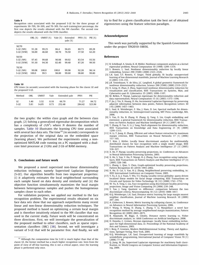
Table 9Recognition rates associated with the proposed S-LE for the three groups of

experiments 30–70%, 50–50%, and 70–30%. For each training/test percentage, the

first row depicts the results obtained with the NN classifier. The second row

depicts the results obtained with the SVM classifier.

ORL (%) UMIST (%) Yale (%) Extended

yale (%)

PF01 (%) PIE (%)

30/70

S-LE (NN) 91.28 99.25 86.4 96.65 80.73 89.28

S-LE (SVM) 56.00 46.60 38.70 76.50 37.50 62.20

50/50

S-LE (NN) 97.45 99.68 90.98 99.92 83.54 93.56

S-LE (SVM) 91.50 94.30 82.40 99.40 87.20 99.50

70/30

S-LE (NN) 99.08 100.0 100.0 99.98 92.28 96.14

S-LE (SVM) 100.0 99.5 98.00 99.60 98.80 99.80

Table 10CPU times (in seconds) associated with the learning phase for the classic LE and

the proposed S-LE.

Method ORL UMIST Yale Extended yale PF01 PIE

LE 1.46 3.32 0.18 66.79 71.27 84.72

S-LE 5.81 14.05 0.73 252.48 284.42 323.96

B. Raducanu, F. Dornaika / Pattern Recognition 45 (2012) 2432–2444 2443

the two graphs: the within class graph and the between classgraph. (2) Solving a generalized eigenvalue decomposition whichhas a complexity of OðN3

Þ where N denotes the number ofsamples. Table 10 illustrates the learning CPU time associatedwith several face data sets. The time10 (in seconds) corresponds tothe projection of the original data on the embedded space(learning phase). We performed the experiments using a non-optimized MATLAB code running on a PC equipped with a dual-core Intel processor at 2 GHz and 2 Gb of RAM memory.

5. Conclusions and future work

We proposed a novel supervised non-linear dimensionalityreduction technique, namely Supervised Laplacian Eigenmap(S-LE). Our algorithm benefits from two important properties:(i) it adaptively estimates the local neighborhood surroundingeach sample based on data density and similarity and (ii) theobjective function simultaneously maximizes the local marginbetween heterogeneous samples and pushes the homogeneoussamples closer to each other.

For validation purposes, we applied our method to the facerecognition problem. The experimental results obtained on sixface data sets show that our approach outperforms many recentlinear and non-linear dimensionality reduction techniques. Theproposed method is based on optimizing a certain local marginand is therefore intuitively related to the NN classifier that wasused in the current study. Future work will be concentrated onthree directions. First, we will investigate the generalization ofthe proposed method to other classifiers, such as sparse repre-sentation classifiers (SRC) [38]. Second, we will investigate avariant of S-LE that will be parameter free. And finally, we will

10 Although the computation time for S-LE is much higher than that of the

classic LE, the former method has a much higher recognition rate. Seen from the

point of view of off-line learning, this is not a critical aspect, since the learning

phase is performed only once.

try to find for a given classification task the best set of obtainedeigenvectors using the feature selection paradigm.

Acknowledgment

This work was partially supported by the Spanish Governmentunder the project TIN2010-18856.

References

[1] B. Scholkopf, A. Smola, K.-R. Muller, Nonlinear component analysis as a kerneleigenvalue problem, Neural Computation 10 (1998) 1299–1319.

[2] S. Roweis, L. Saul, Nonlinear dimensionality reduction by locally linearembedding, Science 290 (5500) (2000) 2323–2326.

[3] L.K. Saul, S.T. Roweis, Y. Singer, Think globally, fit locally: unsupervisedlearning of low dimensional manifolds, Journal of Machine Learning Research4 (2003) 119–155.

[4] J.B. Tenenbaum, V. de Silva, J.C. Langford, A global geometric framework fornonlinear dimensionality reduction, Science 290 (5500) (2000) 2319–2323.

[5] X. Geng, D. Zhan, Z. Zhou, Supervised nonlinear dimensionality reduction forvisualization and classification, IEEE Transactions on Systems, Man, andCybernetics-part B: Cybernetics 35 (2005) 1098–1107.

[6] M. Belkin, P. Niyogi, Laplacian eigenmaps for dimensionality reduction anddata representation, Neural Computation 15 (6) (2003) 1373–1396.

[7] P. Jia, J. Yin, X. Huang, D. Hu, Incremental Laplacian Eigenmaps by preservingadjacent information between data points, Pattern Recognition Letters 30(16) (2009) 1457–1463.

[8] L. Saul, K. Weinberger, F. Sha, J. Ham, D. Lee, Spectral methods for dimen-sionality reduction, in: Semisupervised Learning, MIT Press, Cambridge, MA,2006.

[9] S. Yan, D. Xu, B. Zhang, H. Zhang, Q. Yang, S. Lin, Graph embedding andextension: a general framework for dimensionality reduction, IEEE Transac-tions on Pattern Analysis and Machine Intelligence 29 (1) (2007) 40–51.

[10] T. Zhang, D. Tao, X. Li, J. Yang, Patch alignment for dimensionality reduction,IEEE Transactions on Knowledge and Data Engineering 21 (9) (2009)1299–1313.

[11] H. Li, T. Jiang, K. Zhang, Efficient and robust feature extraction by maximummargin criterion, IEEE Transactions on Neural Networks 17 (1) (2006)157–165.

[12] T. Kim, J. Kittler, Locally linear discriminant analysis for multimodallydistributed classes for face recognition with a single model image, IEEETransactions on Pattern Analysis and Machine Intelligence 27 (3) (2005)318–327.

[13] X. He, P. Niyogi, Locality preserving projections, in: Conference on Advancesin Neural Information Processing Systems, 2003.

[14] X. He, S. Yan, Y. Hu, P. Niyogi, H.-J. Zhang, Face recognition using Laplacian-faces, IEEE Transactions on Pattern Analysis and Machine Intelligence 27 (3)(2005) 328–340.

[15] L. Zhang, L. Qiao, S. Chen, Graph-optimized locality preserving projections,Pattern Recognition 43 (2010) 1993–2002.

[16] X. He, D. Cai, S. Yan, H.-J. Zhang, Neighborhood preserving embedding, in:IEEE International Conference on Computer Vision, 2005.

[17] Y. Fu, Z. Li, J. Yuan, Y. Wu, T.S. Huang, Locality versus globality: query-drivenlocalized linear models for facial image computing, IEEE Transactions onCircuits and Systems for Video Technology 18 (12) (2008) 1741–1752.

[18] W. Yu, X. Teng, C. Liu, Face recognition using discriminant locality preservingprojections, Image and Vision Computing 24 (2006) 239–248.

[19] Y. Tao, J. Yang, Quotient vs. difference: comparison between the twodiscriminant criteria, Neurocomputing 18 (12) (2010) 1808–1817.

[20] K.Q. Weinberger, L.K. Saul, Distance metric learning for large margin nearestneighbor classification, Journal of Machine Learning Research 10 (2009)207–244.

[21] A. Globerson, S. Roweis, Metric learning by collapsing classes, in: Conferenceon Advances in Neural Information Processing Systems, 2006.

[22] F. Wang, X. Wang, D. Zhang, C. Zhang, T. Li, Marginface: a novel facerecognition method by average neighborhood margin maximization, PatternRecognition 42 (2009) 2863–2875.

[23] B. Alipanahi, M. Biggs, A. Ghodsi, Distance metric learning vs. Fisherdiscriminant analysis, in: AAAI Conference on Artificial Intelligence, 2008.

[24] D. Donoho, C. Grimes, Hessian eigenmaps: locally linear embedding techni-ques for high-dimensional data, in: Proceedings of the National Academy ofArts and Sciences, 2003.

[25] I. Borg, P. Groenen, Modern Multidimensional Scaling: Theory and Applica-tions, Springer-Verlag, New York, 2005.

[26] K.Q. Weinberger, L.K. Saul, Unsupervised learning of image manifolds bysemidefinite programming, International Journal of Computer Vision 70 (1)(2006) 77–90.

[27] Q. Jiang, M. Jia, Supervised Laplacian eigenmaps for machinery fault classi-fication, in: World Congress on Computer Science and Information Engineer-ing, 2009.

B. Raducanu, F. Dornaika / Pattern Recognition 45 (2012) 2432–24442444

[28] O. Kouropteva, O. Okun, M. Pietikainen, Supervised locally linear embeddingalgorithm for pattern recognition. in: Pattern Recognition and Image Analy-sis, Lecture Notes in Computer Science, vol. 2652, 2003.

[29] M. Pillati, C. Viroli, Supervised locally linear embedding for classification: anapplication to gene expression data analysis, in: Proceedings of 29th AnnualConference of the German Classification Society, 2005.

[30] Y. Xu, A. Zhong, J. Yang, D. Zhang, LPP solution schemes for use with facerecognition, Pattern Recognition 43 (2010) 4165–4176.

[31] J. Liu, Face Recognition on Riemannian Manifolds, Master’s Thesis, Autono-mous University of Barcelona, 2011.

[32] J. Shi, J. Malik, Normalized cuts and image segmentation, IEEE Transactionson Pattern Analysis and Machine Intelligence 22 (8) (2000) 888–905.

[33] S.X. Yu, J. Shi, Multiclass spectral clustering, in: IEEE International Conferenceon Computer Vision, 2003.

[34] N. Goel, G. Bebis, A. Nefian, Face recognition experiments with randomprojections, in: SPIE Conference on Biometric Technology for Human Identi-fication, 2005.

[35] R. Duda, P. Hart, D. Stork, Pattern Classification, John Wiley and Sons,New York.

[36] S. Yan, D. Xu, B. Zhang, H. Zhang, Graph embedding: a general framework fordimensionality reduction, in: IEEE Conference on Computer Vision and

Pattern Recognition, 2005.[37] X. Qiu, L. Wu, Face recognition by stepwise nonparametric margin maximum

criterion, in: IEEE International Conference on Computer Vision, 2005.[38] J. Wright, A. Yang, A. Ganesh, S. Sastry, Y. Ma, Robust face recognition via

sparse representation, IEEE Transactions on Pattern Analysis and Machine

Intelligence 31 (2) (2009) 210–227.

Bogdan Raducanu received the B.Sc. degree in computer science from the University ‘‘Politehnica’’ of Bucharest, Bucharest, Romania, in 1995 and the Ph.D. degree ‘‘CumLaude’’ from the University of the Basque Country, Bilbao, Spain, in 2001. Currently, he is a senior researcher at the Computer Vision Center in Barcelona, Spain. Hisresearch interests are: computer vision, pattern recognition, machine learning, artificial intelligence, social computing and human–robot interaction. He is the author orco-author of about 60 publications in international conferences and journals. In 2010, he was the leading Guest Editor of Image and Vision Computing journal for a specialissue on ‘Online Pattern Recognition’.

Fadi Dornaika received the Ph.D. in signal, image, and speech processing from the Institut National Polytechnique de Grenoble, France, in 1995. He is currently anIkerbasque research professor at the University of the Basque Country. He has published more than 130 papers in the field of computer vision. His research concernsgeometrical and statistical modelling with focus on 3D object pose, real-time visual servoing, calibration of visual sensors, cooperative stereo-motion, image registration,facial gesture tracking, and facial expression recognition.