a supervised learning approach for dynamic sampling

A Supervised Learning Approach for Dynamic SamplingG.M. Dilshan Godaliyadda1, Dong Hye Ye1, Michael D. Uchic3, Michael A. Groeber3, Gregery T. Buzzard2 and Charles A. Bouman1;1School of ECE, Purdue University, West Lafayette, IN, USA;2Department of Mathematics, Purdue University, West Lafayette, IN, USA;3Air Force Research Laboratory, Materials and Manufacturing Directorate, Wright-Patterson AFB, OH, USA

AbstractSparse sampling schemes have the potential to reduce image

acquisition time by reconstructing a desired image from a sparsesubset of measured pixels. Moreover, dynamic sparse samplingmethods have the greatest potential because each new pixel isselected based on information obtained from previous samples.However, existing dynamic sampling methods tend to be compu-tationally expensive and therefore too slow for practical applica-tion.

In this paper, we present a supervised learning based algo-rithm for dynamic sampling (SLADS) that uses machine-learningtechniques to select the location of each new pixel measurement.SLADS is fast enough to be used in practical imaging applica-tions because each new pixel location is selected using a simpleregression algorithm. In addition, SLADS is accurate becausethe machine learning algorithm is trained using a total reduc-tion in distortion metric which accounts for distortion in a neigh-borhood of the pixel being sampled. We present results on bothcomputationally-generated synthetic data and experimentally-collected data that demonstrate substantial improvement relativeto state-of-the-art static sampling methods.

IntroductionIn conventional point-wise image acquisition, all pixels in a

rectilinear grid are measured. However, in many imaging applica-tions, a high-fidelity pixel measurement could take up to 1 second.Examples of such methods include electron back scatter diffrac-tion (EBSD) microscopy and Raman spectroscopy, which are ofgreat importance in material science and chemistry [1]. Then, ac-quiring a complete set of high-resolution measurements on theseimaging applications becomes impractical.

Sparse sampling offers the potential to dramatically reducethe time required to acquire an image. In this approach, a sparseset of pixels is measured, and the full resolution image is re-constructed from the set of sparse measurements. In addition tospeeding image acquisition, sparse sampling methods also holdthe potential to reduce the exposure of the object being imaged todestructive radiation. This is of critical importance when imagingbiological samples using X-rays, electrons, or even optical pho-tons [2, 3].

Sparse sampling approaches fall into two main categories:static and dynamic. In static sampling, pixels are measured ina pre-defined order. Examples of static sparse sampling meth-ods include random sampling strategies such as in [4], and low-discrepancy sampling [5]. As a result some samples from thesemethods may not be very informative, as they do not take into ac-count the object being scanned. There are static sampling meth-ods based on an a priori knowledge of the object geometry and

sparsity such as [6, 7]. However a priori knowledge is not alwaysavailable for general imaging applications

On the other hand, dynamic sampling (DS) methods adap-tively determine new measurement locations based on the infor-mation obtained from previous measurements. This is a very pow-erful technique since in real applications previous measurementscan tell one a great deal about the object being scanned and alsoabout the best locations for future measurements Therefore, dy-namic sampling has the potential to dramatically reduce the to-tal number of samples required to achieve a particular level ofdistortion in the reconstructed image. An example of a dynamicsampling method was proposed in [8] by Kovacevic et al. Hereinitially an object is measured with a sparse grid. Then, if theintensity of a pixel is above a certain threshold, the vicinity ofthat pixel is measured in higher resolution. However, the thresh-old was empirically chosen for the specific scanner and thus thismethod cannot be generalized for different imaging modalities.

For general applications, a set of DS methods has been pro-posed in previous literature where an objective function is de-signed and the measurements are chosen to optimize that objec-tive function. For instance, dynamic compressive sensing meth-ods [9–11] find the next measurements that maximally reducesthe differential entropy. However, dynamic compressive sensingmethods use an unconstrained projection as a measurement andtherefore are not suitable for point-wise measurements where themeasurement is constrained.

Apart from these methods, application specific DS methodsthat optimize an objective function to find the next measurementhave been developed. One example is [12], where the authorsmodify the optimal experimental design [13] framework to incor-porate dynamic measurement selection in a biochemical network.Seeger et al. in [14] also finds the measurement that reduces thedifferential entropy the most but now to select optimal K-spacespiral and line measurements for magnetic resonance imaging(MRI). In addition, Batenburg et al. [15] propose a DS methodfor binary computed tomography in which the measurement thatmaximizes the information gain is selected. Even though thesemeasurements are constrained they are application specific andtherefore not applicable to general point-wise measurements.

In [16] Godaliyadda et al. propose a DS algorithm for gen-eral point-wise measurements. Here, the authors use a Monte-Carlo simulation method to approximate the conditional vari-ance at every unmeasured location, given previous measurements,and select the pixel with largest conditional variance. However,Monte-Carlo simulation methods such as the Metropolis-Hastingsmethod are very slow and therefore this method is infeasible forreal-time applications. Furthermore, the objective function in thismethod does not account for the change of conditional variance in

©2016 Society for Imaging Science and TechnologyDOI: 10.2352/ISSN.2470-1173.2016.19.COIMG-153

IS&T International Symposium on Electronic Imaging 2016Computational Imaging XIV COIMG-153.1

the entire image with a new measurement.In this paper, we propose a new DS algorithm for point-wise

measurements named supervised learning approach for dynamicsampling (SLADS). The objective of SLADS is to select a newpixel so as to maximally reduce the conditional expectation of thereduction in distortion (ERD) in the entire reconstructed image.In SLADS, we compute the reduction in distortion for each pixelin a training data set, and then find the relationship between theERD and a local feature vector through a regression algorithm.Since we use a supervised learning approach, we can very rapidlyestimate the ERD at each pixel in the unknown testing image.Moreover, we introduce a measure that approximates the distor-tion reduction in the training dataset so that it accounts for thedistortion reduction in the pixel and its neighbors. Since comput-ing the distortion reduction for each pixel during training can beintractable, particularly for large images, this approximation is vi-tal to make the training procedure feasible. Experimental resultson sampling a computationally-generated synthetic EBSD imageand an experimentally-collected image have shown that SLADScan compute a new sample locations very quickly (in the range of5 - 500 ms), and can achieve the same reconstruction distortionas static sampling methods with dramatically fewer samples (2-4times fewer).

Dynamic Sampling FrameworkThe objective in sparse sampling is to measure a sparse set of

pixels in an image and then reconstruct the full resolution imagefrom those sparse samples. Moreover, with sparse dynamic sam-pling, the location for each new pixel to measure will be informedby all the previous pixel measurements.

To formulate the problem, we denote the image we wouldlike to measure as X ∈ RN , where Xr is a pixel at location r ∈ Ω.Furthermore, let us assume that k pixels have been measured at aset of locations S = s(1), · · · ,s(k), and that the correspondingmeasured values and locations are represented by the k×2 matrix

Y (k) =

s(1),Xs(1)

...

s(k),Xs(k)

.

Then from Y (k), we can reconstruct an image X (k), which is ourbest estimate of X given the first k measurements.

Now, if we select Xs as our next pixel to measure, then pre-sumably we can reconstruct a better estimate of the image, whichwe will denote by X (k;s). So then X (k;s) is our best estimate of Xgiven both Y (k) and Xs.

So at this point, our goal is to select the next location s(k+1)that results in the greatest decrease in reconstruction distortion. Inorder to formulate this problem, let D(Xr, Xr) denote the distortionmeasure between a pixel Xr and its estimate Xr, and let

D(X , X) = ∑r∈Ω

D(Xr, Xr) , (1)

denote the total distortion between the image X and its estimateX .

Then using this notation, we may define R(k;s)r to be the lo-

cal reduction in distortion at pixel r that would result from the

measurement of the pixel Xs.

R(k;s)r = D(Xr, X

(k)r )−D(Xr, X

(k;s)r ) (2)

Importantly, the measurement of the pixel Xs does not only reducedistortion at that pixel. It also reduces the distortion at neighbor-ing pixels. So in order to represent the total reduction in distor-tion, we must sum over all pixels r ∈Ω.

R(k;s) = ∑r∈Ω

R(k;s)r (3)

= D(X , X (k))−D(X , X (k;s)) . (4)

Now of course, we do not know what the value of Xs until it ismeasured; so we also do not know the value R(k;s). Therefore, wemust make our selection of the next pixel based on the conditionalexpectation of reduction in distortion which we will refer to as theERD given by

R(k;s) = E[R(k;s)|Y (k)

]. (5)

So with this notation, our goal is to efficiently compute thenext pixel to sample, s(k+1), as the solution to the following opti-mization.

s(k+1) = arg maxs∈Ω\S

(R(k;s)

)(6)

Once we measure the location Xs(k+1) , then we form the new mea-surement vector

Y (k+1) =

[Y (k)

s(k+1),Xs(k+1)

], (7)

and we repeat the process recursively until the stopping conditiondiscussed below is achieved.

Supervised Learning Approach for DynamicSampling (SLADS)

Our SLADS approach will be based on supervised learning.To do this, we will use training data in an off-line procedure topredict the value of R(s) from the available data Y . Notice thatin this section, we suppress the dependance on the time index ksince the training is done in a batch process.

More specifically, we will compute the ERD by fitting a re-gression function, f , so that

R(s) = f θs (Y ) . (8)

Here f θs (·) denotes a non-linear regression function determined

through supervised learning, and θ is the parameter vector thatwe must estimate in the learning process.

Now in order to train f θs (·), we will first construct a training

data base containing many corresponding pairs (R(s),Y ). Noticethat since R(s) is the reduction in distortion it requires knowledgeof the true image X . However, since this is an off-line training pro-cedure, this information is available. Also, the regression func-tion, f θ

s (Y ), will compute the required conditional expectationrequired for R(s).

While it is possible to compute the corresponding value ofR(s) for each possible set of sample measurements Y , this is very



http://dx.doi.org/10.2352/ISSN.2470-1173.2016.19.COIMG-153


computationally expensive since it requires that one compute afull reconstruction, Xs, for each of the training pairs. In practice,we will use a large number of training samples, so we will intro-duce an approximation to R(s) that will dramatically reduce thecomputation required for training. Our approximation is given by

R(s)r ≈ h(s)r D

(Xr, Xr

), (9)

where

h(s)r = exp− c

2(σ (s))2‖r− s‖2

(10)

and where c is a user selectable parameter and σ (s) is the distancebetween the pixel s and the nearest previously measured pixel.More formally, σ (s) can be computed as

σ(s) = min

t∈S‖s− t‖ , (11)

where S is the set of measured locations.So intuitively, the function h(s)r is a Gaussian shaped weight-

ing with an approximate radius σ (s) where σ (s) is the distancebetween s and the nearest measurement. Figure 1 illustrates theshape of the function h(s)r . Figures 1(b) and (c) illustrate the shapeof h(s)r for two different cases. In (b), the pixel s1 is further fromthe nearest measured pixel; and in (c), the pixel s2 is nearer.

The interpretation of equation (9) is that the reduction of er-ror at the pixel r is proportional to the initial distortion at the lo-cation r multiplied by the weighting factor h(s)r . When r = s, thenh(s)s = 1 and we have that

R(s)s = D

(Xs, Xs

). (12)

However, as r becomes more distant from the pixel being mea-sured s, then the reduction in distortion will be attenuated by theweight h(s)r < 1.

s1 σ (s1 )

s2σ (s2 )

(a) Measurements

s1

(b) h(s1)r

s2

(c) h(s2)r

Figure 1. Illustrates the shape of the function h(s)r . (b) and (c) illustrate the

shape of h(s)r for two different values of σ (s), σ (s1) and σ (s2) respectively. Note

that the distance from pixel s1 to the nearest measurement is larger than the

distance from pixel s2 to the nearest measurement. Therefore, σ (s1) > σ (s2).

As a result the kernel h(s1)r is spread over a wider region when compared to

the kernel h(s2)r .

Using this approximation, we can now compute an approxi-mation to the TRD given by

R(s) = ∑r∈Ω

R(s)r ≈ ∑

r∈Ω

h(s)r D(Xr, Xr

). (13)

From this point on, we will use this approximation to R(s) in allour computations.

In order to train the SLADS algorithm, we must estimate theregression function f θ

s (Y ) using machine learning techniques. Todo this, let Vs denote a p-dimensional feature row vector extractedfrom the data Y . In our example, this feature vector is formedby the 6 scalar descriptors Zs,1,Zs,2, . . .Zs,6 listed in Table 1. Inparticular,

Vs =[1,Zs,1, . . . ,Zs,6,Z

2s,1,Zs,1Zs,2, . . . ,Z2

s,6

], (14)

so that p = 28.

Measures of gradientsThe gradient in the x-direction.

Zs,1 = D(Xsx+ , Xsx−

)The distortion between the esti-

mate of the pixel adjacent to s in the

positive x-direction, Xsx+ , and the

estimate of the pixel adjacent to s

in the negative x-direction, Xsx− .

The gradient in the y-direction.

Zs,2 = D(Xsy+ , Xsy−

)The distortion between the esti-

mate of the pixel adjacent to s in the

positive y-direction, Xsy+ , and the

estimate of the pixel adjacent to s

in the negative y-direction, Xsy− .

Measures of standard deviation

Zs,3 =

√1L ∑

r∈∂ sD(Xr, Xs

)2

Here ∂ s is the set containing the

indices of the L nearest measure-

ments to s.

Zs,4 = ∑r∈∂ s

w(s)r D

(Xr, Xs

)

Here w(s)r =

1‖s−r‖2

∑u∈∂ s

1‖s−u‖2

.

Measures of density of measurements

Zs,5 = minr∈∂ s‖s− r‖2

The distance from s to the closest

measurement.

Zs,6 =1+A(s;λ )

1+A∗(s;λ )

Here A(s;d) is the area of a circle λ%

the size of the image around pixel s,

A∗(s;λ ) is the measured area inside

A(s;λ ).

Table 1: List of descriptors used to construct the feature vec-tor. There are three main categories of descriptors: measuresof gradients, measures of standard deviation, and measuresof density of measurements surrounding the pixel s.

However, more generally Vs may be any set of local descrip-tors that can be used to predict the value of R(s). From this featurevector, we can then compute the ERD using a linear predictor withthe following form.

R(s) = f θs (Y ) =Vs θ (15)

We can estimate the parameter θ by solving the following least-squares regression

θ = arg minθ∈Rp

‖R−V θ‖2 , (16)

where R is an n-dimensional column vector formed by

R =[R(s1), . . . ,R(sn)

], (17)





and V is given by

V = [Vs1 , . . . ,Vsn ] . (18)

So together, (R,V ) consist of n training pairs, (Rsi ,Vsi)ni=1, that

are extracted from separate training data in an off-line procedure.The parameter θ is then given by

θ =(V tV

)−1 V tR . (19)

Once the θ is estimated, then it can be used for fast on-linedynamic sampling by selecting the pixel that maximizes the ERDgiven by


(V (k)

s θ

), (20)

where V (k)s denotes the feature vector extracted from the measure-

ments Y (k) for a possible measurement of the pixel Xs. The pseudocode for SLADS is shown in Figure (2).

function Y (K) ← SLADS(Y (k), θ ,k)

S ←s1,s2, . . .sk

while Stopping condition not met do

for do∀s ∈ Ω\S

Extract V (k)s

R(k;s)←V (k)s θ

end for


(R(k;s)

)

Y (k+1)←

[Y (k)

s(k+1),Xs(k+1)

]

S ←S ∪ s(k+1)

k← k+1

end while

K← k

end function

Figure 2. SLADS algorithm in pseudo code. The inputs to the function are

the initial measurements Y (k), the coefficients needed to compute the ERD,

found in training, θ , and k the number of measurements. When the stopping

condition is met the function will output the selected set of measurements

Y (K).

Stopping Condition for SLADSIdeally, dynamic sampling should stop when the normalized

reconstruction distortion (NRD) reaches a predetermined thresh-

old.

1|Ω|

D(X , X

)≤ T (21)

However, since we do not know the underlying object X , it is notpossible to know the NRD.

In our implementation, at each step of SLADS we compute arunning average of the reconstruction distortion between the mea-sured pixel and the estimate of that pixel from previous measure-ments. Then we use a threshold on this quantity to decide whento stop sampling.

To do this, we apply the following recursion, after each newsample is taken,

ε(k) = αε

(k−1)+(1−α)D(

Xs(k) , X(k−1)s(k)

), (22)

where α is a user selected parameter that determines the amountof temporal smoothing. Intuitively, the value of ε(k) measuresthe average level of distortion in the measurements. So a largevalue of ε(k) indicates that more samples need to be taken, and asmaller value indicates that the reconstruction is accurate and thesampling process can be terminated.

So therefore, we must find the threshold T (T ) on ε(k) thatcorresponds to the desired threshold T on the NRD. For this pur-pose, we perform dynamic sampling on a known image X . Westop sampling when the NRD ≤ T , and record the value of ε(k).Next, we define

K(T ) = maxk

k :

1|Ω|

D(

X , X (k))≤ T,k ∈ 1,2, . . .N

.

(23)

Now we repeat the process for M different images and recordε(K

m(T )) for each image m ∈ 1,2, . . .M. Then we averageε(K

m(T )) over the M experiments to find T .

T (T ) =1M

M

∑m=1

ε(Km(T )) (24)

Typically, T (T ) is a decreasing function of T , although this is notguaranteed.

During the first few steps of dynamic sampling the value ofε(k) can be relatively small. Hence, using only the threshold Tcan lead to premature termination. However, during the first stepsthe function ε(k) increases with k. We take advantage of this factto design a second condition of stopping. The condition is that theaverage change of ε(k) over J steps has to be non-positive i.e. ε(k)

on average is decreasing with k over J steps.

J

∑j=1

[ε(k)− ε

(k− j)]≤ 0 (25)

ResultsIn this section we compare SLADS with two static sam-

pling methods — low-discrepancy sampling (LS) and Ran-dom Sampling (RS). We performing sampling experiments ona computationally-generated synthetic EBSD image and on anexperimentally-collected image. We compare the sampling meth-ods by plotting the NRD versus the number of samples and by the





visual quality of the reconstructed images. The method we use toconstruct the training database for SLADS is detailed below.

We start by selecting M training images

X1,X2, . . .XM.Now from image X1 we select 5% of pixels using a uniform ran-dom distribution and consider them as the measurements Y . Thenfor all the unmeasured locations in X1 we compute (R(s),Vs) andsave this vector in the training database. Figure 3 illustrates thisprocedure for the case when p% is measured. We then repeat thisprocess for the same image but now select 10,20,40, and 80% ofpixels as measurements. Next, we repeat the same process for theother training images.

Training Image

Measured Image (p% measured)

Training Database

Extract Vs ∀s ∈ Ω \ S

Compute R(s )

∀s ∈ Ω \ S

Figure 3. Illustration of how we extract one set of entries from one image to

create the training database. We first select p% of the pixels in the image and

consider them as measurements Y . Then for all unmeasured pixel locations

(s ∈ Ω\S ) we extract a feature vector Vs and compute R(s). Here again Ω

is the set of all locations in the training image and S is the set of measured

locations. All these pairs of(Vs,R(s)

)are then stored in the training database.

For all the experiments in the next two sections we start bysampling 1% of the image, according to low-discrepancy sam-pling. Then we continue RS and LS until 20% of the image ismeasured, and SLADS until a specified stopping condition is met.

Comparing SLADS with Static Sampling Methodson Computationally-Generated Synthetic EBSDImage

In this section we compare SLADS with LS and RS by sam-pling a computationally-generated synthetic EBSD image gener-ated using the Dream.3D software [17]. This image, shown inFigure 5, has a resolution of 512× 512 pixels. This image con-tains discretely labeled regions each corresponding to differentcrystal orientations. Therefore in this experiment, we define thedistortion D(a,b) between two values a and b as,

D(a,b) =

0 a = b

1 a 6= b.(26)

The training images for SLADS were also generated usingthe Dream.3D software and have the same resolution as the testimage. These images are shown in Figure 4(a). To compute R(s)

we use c = 8 in equation (9) and perform reconstructions usingweighted mode interpolation.

The weighted mode interpolation of a pixel s is Xr∗ if

r∗ = argmaxr∈∂ s

∑

t∈∂ s

[(1−D(Xr,Xt))w(s)

r

]. (27)

where,

w(s)r =

1‖s−r‖2

∑u∈∂ s

1‖s−u‖2

. (28)

For this experiment we let |∂ s| = 10. We use weighted modeinterpolation to compute reconstructions needed to for descriptorcomputation as well.

Also, for this experiment the desired NRD was set to 2×10−5 (T = 2×10−5). To find the corresponding stopping thresh-old T on ε(k) we use the set of images shown in Figure 4(b).To compute ε(k) we set α = 0.99 and once more use weightedmode interpolation for interpolations. The threshold we foundwas 0.0041 (T = 0.0041).

(a) Discrete: Training Images

(b) Discrete: Images to find stopping condition

Figure 4. Training images and images used to find stopping condition for

SLADS experiment on a computationally-generated synthetic EBSD image.

The first set of images, (a), were used to find the regression parametersˆT heta. The second set of images, (b), were used to find the stopping thresh-

old.

We display results for sampling the computationally-generated synthetic EBSD image in Figure 5. Figure 5(d) showsthe reconstruction performed after SLADS stops, which in thiscase is after 6.94% of the image is sampled. Figures 5(b) and 5(c)show the reconstructions performed from the same percentage ofsamples (6.94%) acquired using RS and LS respectively. Figure5(e) shows the NRD versus the percentage of samples, and finally5(f-h) show the measurement masks corresponding to reconstruc-tions (b)-(d).





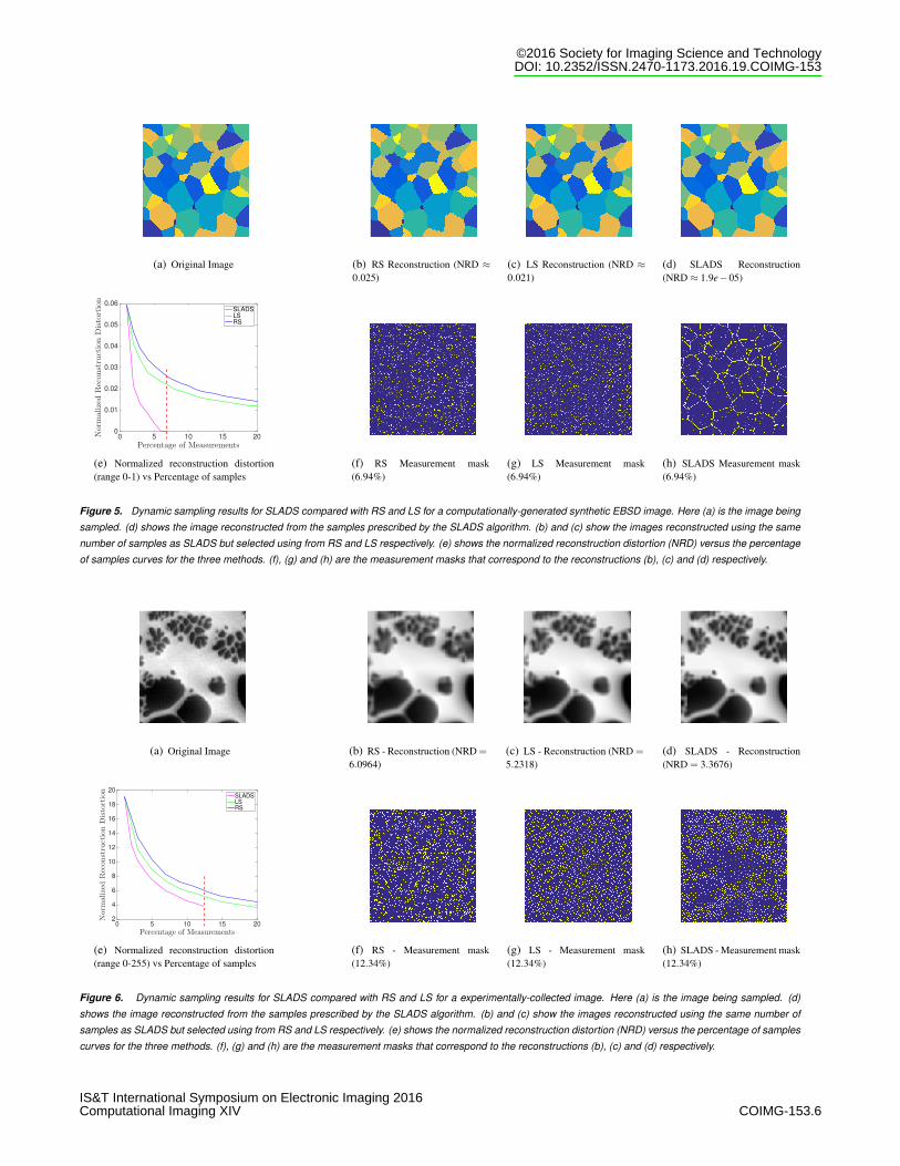
(a) Original Image (b) RS Reconstruction (NRD ≈0.025)

(c) LS Reconstruction (NRD ≈0.021)

(d) SLADS Reconstruction(NRD ≈ 1.9e−05)

Percentage of Measurements0 5 10 15 20N

orm

alizedReconstructionDistortion

0

0.01

0.02

0.03

0.04

0.05

0.06SLADS

LS

RS

(e) Normalized reconstruction distortion(range 0-1) vs Percentage of samples

(f) RS Measurement mask(6.94%)

(g) LS Measurement mask(6.94%)

(h) SLADS Measurement mask(6.94%)

Figure 5. Dynamic sampling results for SLADS compared with RS and LS for a computationally-generated synthetic EBSD image. Here (a) is the image being

sampled. (d) shows the image reconstructed from the samples prescribed by the SLADS algorithm. (b) and (c) show the images reconstructed using the same

number of samples as SLADS but selected using from RS and LS respectively. (e) shows the normalized reconstruction distortion (NRD) versus the percentage

of samples curves for the three methods. (f), (g) and (h) are the measurement masks that correspond to the reconstructions (b), (c) and (d) respectively.

(a) Original Image (b) RS - Reconstruction (NRD =

6.0964)(c) LS - Reconstruction (NRD =

5.2318)(d) SLADS - Reconstruction(NRD = 3.3676)

Percentage of Measurements0 5 10 15 20

Norm

alizedReconstructionDistortion

2

4

6

8

10

12

14

16

18

20SLADS

LS

RS

(e) Normalized reconstruction distortion(range 0-255) vs Percentage of samples

(f) RS - Measurement mask(12.34%)

(g) LS - Measurement mask(12.34%)

(h) SLADS - Measurement mask(12.34%)

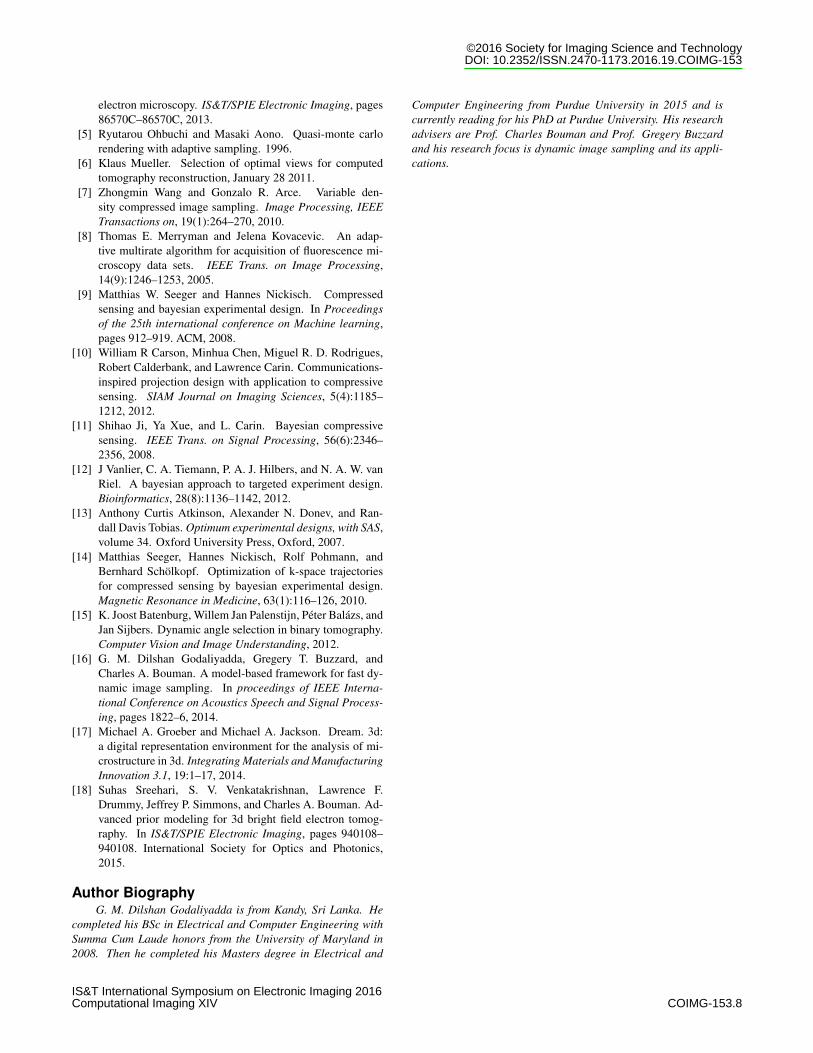
Figure 6. Dynamic sampling results for SLADS compared with RS and LS for a experimentally-collected image. Here (a) is the image being sampled. (d)

shows the image reconstructed from the samples prescribed by the SLADS algorithm. (b) and (c) show the images reconstructed using the same number of

samples as SLADS but selected using from RS and LS respectively. (e) shows the normalized reconstruction distortion (NRD) versus the percentage of samples

curves for the three methods. (f), (g) and (h) are the measurement masks that correspond to the reconstructions (b), (c) and (d) respectively.





(a) Continuous: Training Images (b) Continuous: Imagesto find stopping condition

Figure 7. Training images and images to find stopping condition for SLADS

simulations on an experimentally-collected image . The first set of images,

(a), were used to find the regression parameters ˆT heta. The second set of

images, (b), were used to find the stopping threshold.

It is clear from Figure 5 that the reconstruction from samplescollected using SLADS is superior to reconstructions from sam-ples collected using RS and LS. The difference between the algo-rithms is most noticeable along the boundaries between the differ-ent grains. Furthermore, from Figure 5(e) we see that the NRD de-creases more rapidly with SLADS. SLADS stops when the NRDis below 2×10−5, thereby validating the stopping threshold.

Comparing SLADS with Static Sampling Methodson Experimentally-Collected Image

In this section we use SLADS, LS and RS to sample theexperimentally-collected image shown in Figure 6(a). The valuesin the testing and training images vary from 0 to 255. Therefore,for this experiment, we define the distortion D(a,b) between twovalues a and b as,

D(a,b) = |a−b|. (29)

The training images used for this experiment are shown inFigure 7. The training images as well as the testing image wereprovided by Ali Khosravani & Prof. Surya Kalidindi from Geor-gia Institute of Technology.

In training, to compute R(s) we set c = 4 and perform re-constructions using the Plug & Play algorithm [18]. However, tocompute the reconstructions for descriptor computations we useweighted mean interpolation instead of Plug & Play. The reasonwe do not use the Plug & Play algorithm when computing the fea-ture vector is because it is slow, and will therefore effect the speedof SLADS. We define the weighted mean for a location s

Xs = ∑r∈∂ s

w(s)r Yr. (30)

For this experiment we let |∂ s|= 10.In this experiment we set the desired NRD to 5 (T = 5). The

images used to find the stopping threshold are shown in Figure7(b). Again, to compute ε(k) we use α = 0.99. The stoppingthreshold was found to be 13.0815 (T = 13.0815).

We display the dynamic sampling results in Figure 6. Fig-ure 6(d) shows the reconstruction performed after SLADS stops,when 12.34% of the image is sampled. Figures 6(b) and 6(c)show the reconstructions performed from the same percentage ofsamples (12.34%) acquired using RS and LS respectively. Here,the reconstructions are performed using the Plug & Play algo-rithm [18]. Figure 6(e) shows the normalized reconstruction dis-tortion (NRD) versus the percentage of samples, and finally 6(f-h) show the measurement masks corresponding to reconstructions(b)-(d).

From Figure 6(b)-(d) we can see that the reconstructionsfrom samples collected using SLADS have better boundary defi-nition between the white and dark regions when compared to thereconstructions from samples collected using RS and LS. FromFigure 6(e) we again see that the normalized reconstruction dis-tortion (NRD) decreases more rapidly with SLADS. Furthermore,we can also see that when SLADS stops the NRD is below 5 asexpected.

ConclusionsIn this paper, we presented a framework for dynamic sam-

pling that can be optimized according to the class of im-age. Furthermore, the SLADS algorithm is very fast, andthe reconstructions resulting from the sampled images showsubstantial improvement over static sampling schemes. Forthe computationally-generated synthetic EBSD image, SLADSachieves a reconstruction distortion below 10−5, with only 6.94%of the image sampled, while for RS and DS, the reconstructiondistortion is above 10−2 even with 20% of the image sampled. Forthe experimentally-collected image SLADS reaches a reconstruc-tion distortion less than 4 with only 13% of the image sampled,while LS requires approximately 18% for the same distortion andRS is above 4 even after 20% of the image is sampled.

ACKNOWLEDGMENTSThe authors acknowledge support from the Air Force Of-

fice of Scientific Research (MURI - Managing the Mosaic ofMicrostructure, grant # FA9550-12-1-0458) and from the AirForce Research Laboratory Materials and Manufacturing direc-torate (Contract # FA8650-10-D-5201-0038). The authors alsothank Ali Khosravani & Prof. Surya Kalidindi, Georgia Instituteof Technology for providing the images used for dynamic sam-pling simulation on an experimentally-collected image.

References[1] Kumar M. Adams B.L. Field D.P. Schwartz, A.J. Electron

Backscatter Diffraction in Materials Science. Springer US,2009.

[2] R. Smith-Bindman, J. Lipson, and R. Marcus. Radiationdose associated with common computed tomography ex-aminations and the associated lifetime attributable risk ofcancer. Archives of Internal Medicine, 169(22):2078–2086,2009.

[3] R. F Egerton, P. Li, and M. Malac. Radiation damage in thetem and sem. Micron, 35(6):399 – 409, 2004. InternationalWuhan Symposium on Advanced Electron Microscopy.

[4] Hyrum S. Anderson, Jovana Ilic-Helms, Brandon Rohrer,Jason Wheeler, and Kurt Larson. Sparse imaging for fast





electron microscopy. IS&T/SPIE Electronic Imaging, pages86570C–86570C, 2013.

[5] Ryutarou Ohbuchi and Masaki Aono. Quasi-monte carlorendering with adaptive sampling. 1996.

[6] Klaus Mueller. Selection of optimal views for computedtomography reconstruction, January 28 2011.

[7] Zhongmin Wang and Gonzalo R. Arce. Variable den-sity compressed image sampling. Image Processing, IEEETransactions on, 19(1):264–270, 2010.

[8] Thomas E. Merryman and Jelena Kovacevic. An adap-tive multirate algorithm for acquisition of fluorescence mi-croscopy data sets. IEEE Trans. on Image Processing,14(9):1246–1253, 2005.

[9] Matthias W. Seeger and Hannes Nickisch. Compressedsensing and bayesian experimental design. In Proceedingsof the 25th international conference on Machine learning,pages 912–919. ACM, 2008.

[10] William R Carson, Minhua Chen, Miguel R. D. Rodrigues,Robert Calderbank, and Lawrence Carin. Communications-inspired projection design with application to compressivesensing. SIAM Journal on Imaging Sciences, 5(4):1185–1212, 2012.

[11] Shihao Ji, Ya Xue, and L. Carin. Bayesian compressivesensing. IEEE Trans. on Signal Processing, 56(6):2346–2356, 2008.

[12] J Vanlier, C. A. Tiemann, P. A. J. Hilbers, and N. A. W. vanRiel. A bayesian approach to targeted experiment design.Bioinformatics, 28(8):1136–1142, 2012.

[13] Anthony Curtis Atkinson, Alexander N. Donev, and Ran-dall Davis Tobias. Optimum experimental designs, with SAS,volume 34. Oxford University Press, Oxford, 2007.

[14] Matthias Seeger, Hannes Nickisch, Rolf Pohmann, andBernhard Scholkopf. Optimization of k-space trajectoriesfor compressed sensing by bayesian experimental design.Magnetic Resonance in Medicine, 63(1):116–126, 2010.

[15] K. Joost Batenburg, Willem Jan Palenstijn, Peter Balazs, andJan Sijbers. Dynamic angle selection in binary tomography.Computer Vision and Image Understanding, 2012.

[16] G. M. Dilshan Godaliyadda, Gregery T. Buzzard, andCharles A. Bouman. A model-based framework for fast dy-namic image sampling. In proceedings of IEEE Interna-tional Conference on Acoustics Speech and Signal Process-ing, pages 1822–6, 2014.

[17] Michael A. Groeber and Michael A. Jackson. Dream. 3d:a digital representation environment for the analysis of mi-crostructure in 3d. Integrating Materials and ManufacturingInnovation 3.1, 19:1–17, 2014.

[18] Suhas Sreehari, S. V. Venkatakrishnan, Lawrence F.Drummy, Jeffrey P. Simmons, and Charles A. Bouman. Ad-vanced prior modeling for 3d bright field electron tomog-raphy. In IS&T/SPIE Electronic Imaging, pages 940108–940108. International Society for Optics and Photonics,2015.

Author BiographyG. M. Dilshan Godaliyadda is from Kandy, Sri Lanka. He

completed his BSc in Electrical and Computer Engineering withSumma Cum Laude honors from the University of Maryland in2008. Then he completed his Masters degree in Electrical and

Computer Engineering from Purdue University in 2015 and iscurrently reading for his PhD at Purdue University. His researchadvisers are Prof. Charles Bouman and Prof. Gregery Buzzardand his research focus is dynamic image sampling and its appli-cations.





a supervised learning approach for dynamic sampling

Documents